San ~r:, Dig, A915-00 V4

0n Technical Document 167800 October 1989

Optimization of GaussianBeam Widths in AcousticPropagation

D. F. Gordon

D TICS ELECTE II

DEC15 1989

E D

Approved for public release; distribution Is unlimited.

89 12 14 09

NAVAL OCEAN SYSTEMS CENTERSan Diego, California 92152-5000

J. D. FONTANA, CAPT, USN R. M. HILLYER

Commander Technical Director

ADMINISTRATIVE INFORMATION

This work was conducted under project RJ14C32 of the Wide Area Undersea Surveil-lance Block Program (NO3A). Block N03A is managed by the Naval Ocean Systems Center,San Diego, CA 92152-5000 under the guidance and direction of the Office of Naval Technol-ogy, Arlington; VA 22217. The work was funded under program element 06023414N and wasperformed by members of the Acoustic Analysis Branch, Code 711, NOSC.

Released by Under authority ofE. F. Rynne, Jr., Head T. F. Ball, HeadAcoustic Analysis Branch Acoustic Systems and

Technology Division

FS

REPORT DOCUMENTATION PAGEPublic reporting burden for Vt clecton of A tioni k is etiaed o averag I hour per reponh. Wckuing Wne O"r rrnm " In . sirAft daa soma. l ienganmaintaining the data needed, and conM*Wn and re wft the lecion of Imtion. Sand commenW regarding th* burden heirln or" any 4sped dN* aOle fti m l ,ini. dingsuggestionsfor reducing Oti burden. ta0eellingion Heaiquaiters Senrls. Directorate tar Intannallon Operationsnd Repors. 1215.1loen Dl"Iglw. Sub 1204. A1ngtn.VA 220-430and to the Office of aamie n Wdgt wof Reduction Pod0704-0188). Wasit on, 00 20503.__________________________

1 AGENCY USE ONLY Leave M" 2. REPORT DATE 3. REPOR TYPE AND DATESC EROI

October 1989 Final

4 TITLE AND SUBTITLE 5 FUNDN NUIAI

OPTIMIZATION OF GAUSSIAN BEAM WIDTHS IN ACOUSTIC PROPAGATION PE: 0602314NWU: DN308 105

8 AUTHOR(S)

D. F. Gordon

7 PERFORMING ORGANIZATION NAME(S) AND ADORESS(ES) S. PERFORMING ORGANIZATIONREPORT NUMBER

Naval Ocean Systems CenterSan Diego, CA 92152-5000 NOSC TD 1678

9 SPONSORING, ONTORING AGENCY NAME(S) AND ADORESS(ES) 10. SPONSORINGMONITORtNAGENCY REPORT NUMBER

Office of Naval TechnologyArlington, VA 22217

11 SUPPLEMENTARY NOTES

I 2 DISTRIBUTION/AVAILALITY STATEMENT 12b. DISTRIBJTION CODE

Approved for public release; distribution is unlimited.

13 ABSTRACT PlAunurl 23 words)

This report outlines a beam-width minimization technique applied to a Gaussian beam model.

Accession For

NTIS GRA&IDTIC TABUnannouncedJustificatio

By

Distribution/

Availability Codes

Avail and/or

Dist Special

14 SUBJECT TERMS 15 NUMBER OF PAGES

22gaussian beams 16 PRICE cODEbeam widths

17 SECURITY CLASSiFICATION Ia SECuRITY CLASSIFICATION i SECURIYCLASSIFICATION 20 LTATION OF ABSTRACTOF REPORT OF THIS PAGE OF ABS'TIACT

UNCLASSIFIED UNCLASSIFIED UNCLASSIFIED

NSN 7540-01-280-56MO Standard torn 2W

CONTENTS

1.0 INTRODUCTION ................................................ 1

2.0 REVIEW OF GAUSSIAN BEAMS ................................... 1

3.0 OPTIMIZATION OF BEAM WIDTH ................................ 3

4.0 PROGRAMMING CONSIDERATIONS .............................. 6

5.0 EXAM PLES ..................................................... 7

6.0 SUM M ARY ..................................................... 8

7.0 RECOMMENDATIONS ........................................... 9

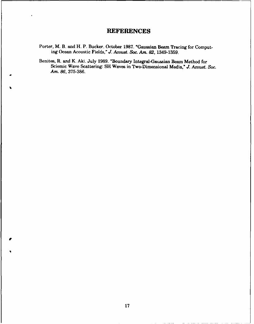
8.0 REFERENCES .................................................. 17

FIGURES

1. A ray path having the source at 4.30 below the horizontal withthe corresponding values of beam functions p and q. Both real andimaginary parts are shown. The ordinates of both imaginaryp andq are arbitrary, being chosen here to match their counterparts .......... 10

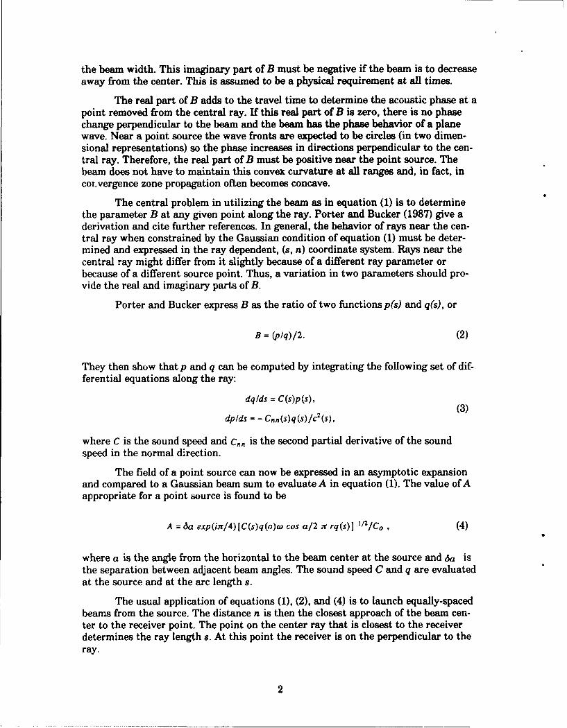
2. A ray path leaving the source at 4.30 above the horizontal withcorresponding values of beam functions p and q ...................... 11

3. A ray path leaving the source at 8.60 below the horizontal withcorresponding values of beam functions p and q ...................... 12

4. Rays from a 1000-m deep source in a Munk canonical sound-speedprofile. Convergence zone 1 is shown ............................... 13

5. Comparison of propagation losses for a 100-m source and 800-mreceiver at 50 Hz as computed by a normal-mode model (solidline) and a Gaussian-beam model (broken line) ....................... 14

6. Comparison of propagation losses for a 300-m source and 150-mreceiver at 50 Hz. Normal-mode . (solid line), Gaussian beamswith minimized widths (broken ,-1 -' andard Gaussian beams(points) ........................ .............................. 14

7. Location of beam centers at points perpendicular to receiver at150-m depth, 61-km range. Some individual beam positions areshown by points. Absolute value of acoustic pressures at the receiverfor the beams whose centers are shown above are shown in thelower two panels as propagation losses .............................. 15

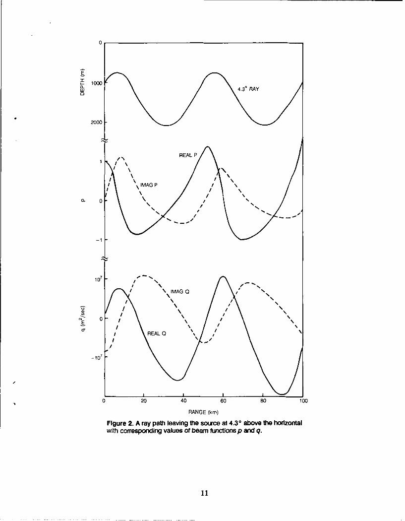
8. Sound pressures of beams as in figure 7, but for standard beamsw ith constant E ................................................. 16

i

1.0 INTRODUCTION

The use of Gaussian beams to compute wave propagation phenomena is a fieldof current interest and activity. Porter and Bucker (1987) supply an extensive list ofreferences. More recent references can be found in Benites and Aki (1989). Gaussianbeams can be traced as rays in range-dependent media providing not only propagationloss, but travel times, multipath structure, and frequency dependence. The well-known ray theory problems of caustics and shadow zones are treated automatically.

This report outlines a beam width minimization technique applied to a Gauss-ian beam model developed by Dr. H. P. Bucker. Porter and Bucker (1987) gives theformulation upon which the technique is built. A free parameter E (caffe- -in Porterand Bucker, 1987) is usually determined in a heuristic manner. Here, it is shown thatthe minimization of beam width assigns a precise value to E. Examples are givenshowing that the minimized beams give good propagation losses in some cases.

A case is also shown in which the standard Gaussian beams give poor resultsand the minimized beams give even worse results. The problem appears to arise inbeams that pass near boundaries. This problem will have to be corrected before afinal judgment can be made on the validity of minimum-width beams.

Gaussian beam cross-sectional intensities and curvature are controlled by twofunctions, p and q. Several examples of these functions are plotted in this report andtheir nature is clarified.

In section 2.0 of this report the parts of Gaussian beam theory used here arereviewed. The following sections then discuss the beam minimization and show exam-ples.

2.0 REVIEW OF GAUSSIAN BEAMS

The Gaussian beam theory and notation used here is that reported by Porterand Bucker (1987). In this section some equations from Porter and Bucker (1987)that are used in later sections will be presented.

A Gaussian beam is assumed to have the form

w(s,n) =A(s,z) exp {-ico [ t(s) + Bn2 I } (1)

where w is the sound pressure, s is the arc length along a ray, n is the normal dis-tance from the ray, zo is the depth of the point source, (9 is the angular frequency,and t is the travel time along the ray. Thus, the Gaussian beam in the current view isinseparably tied to ray theory. The center of the beam is a ray which defines s and t;the field u at a point in space is determined by the minimum distance, n, from thecentral ray.

The parameter B is a complex number. The imaginary part defines the rate atwhich the beam acoustic pressure decreases from the center, or equivalently defines

the beam width. This imaginary part of B must be negative if the beam is to decreaseaway from the center. This is assumed to be a physical requirement at all times.

The real part of B adds to the travel time to determine the acoustic phase at apoint removed from the central ray. If this real part of B is zero, there is no phasechange perpendicular to the beam and the beam has the phase behavior of a planewave. Near a point source the wave fronts are expected to be circles (in two dimen-sional representations) so the phase increases in directions perpendicular to the cen-tral ray. Therefore, the real part of B must be positive near the point source. Thebeam does not have to maintain this convex curvature at all ranges and, in fact, incor vergence zone propagation often becomes concave.

The central problem in utilizing the beam as in equation (1) is to determinethe parameter B at any given point along the ray. Porter and Bucker (1987) give aderivation and cite further references. In general, the behavior of rays near the cen-tral ray when constrained by the Gaussian condition of equation (1) must be deter-mined and expressed in the ray dependent, (s, n) coordinate system. Rays near thecentral ray might differ from it slightly because of a different ray parameter orbecause of a different source point. Thus, a variation in two parameters should pro-vide the real and imaginary parts of B.

Porter and Bucker express B as the ratio of two functions p(s) and q(s), or

B = (p/q)/2. (2)

They then show that p and q can be computed by integrating the following set of dif-ferential equations along the ray:

dq/ds = C(s)p(s), (3)dpds = - C, (s)q(s) Ic2(S),

where C is the sound speed and c,, is the second partial derivative of the soundspeed in the normal direction.

The field of a point source can now be expressed in an asymptotic expansionand compared to a Gaussian beam sum to evaluate A in equation (1). The value of Aappropriate for a point source is found to be

A = a exp(ix/4)[C(s)q(o)o cos a/2 x rq(s)] 1/2/Co , (4)

where a is the angle from the horizontal to the beam center at the source and 6a isthe separation between adjacent beam angles. The sound speed C and q are evaluatedat the source and at the arc length s.

The usual application of equations (1), (2), and (4) is to launch equally-spacedbeams from the source. The distance n is then the closest approach of the beam cen-ter to the receiver point. The point on the center ray that is closest to the receiverdetermines the ray length s. At this point the receiver is on the perpendicular to theray.

2

A beam will contribute to any receiver, although a distance between beam andreceiver can usually be found where the beam contribution is negligibly small. Thefield at a given point will usually consist of contributions from a number of beamsthat are sufficiently close to the receiver. If the beams can be made narrower, fewerbeams will contribute to a given receiver point. This depends upon p/q and theirstarting values.

For the present let

p(O) = 1 and q(O) =iE0 . (5)

The function p starts at a real number and q starts with a pure imaginary con-stant E0 . Following Porter and Bucker (1987), in a medium with constant soundspeed C, the rays are straight lines and equation (3) gives

p(s) = I and q(s) = Cos + iE0 , (6)

because c,, is zero. Thus, in a uniform medium the beam width will depend upon thestarting value Eo near the source but at long distances from the source (large s) willbecome approximately proportional to s. When Cos = Eo, the two terms have aboutequal effect. This cross-over point will turn out later to be related to the optimumbeam width.

3.0 OPTIMIZATION OF BEAM WIDTH

Porter and Bucker (1987) suggest values of Eo as starting values for q. Theseare functions of the beam spacing 6a and make the beams overlap at their lie downpoints in the far field. These, and similar values of E", were tried in a convergencezone environment. It was found that similar sound fields were computed no matterwhat value of Eo was used. Any selected E,, resulted in values ofp and q, and there-fore values of A and B which gave a similar value for the acoustic field. Propagationlosses were generally within 3 dB of each other. These observations led to a closerexamination of the functions p and q, and to the concept that E0 could be chosen in-dependently for each beam and was not a true constant. The subscript o will there-fore be omitted from E when used ir. this context. Observation showed that p and qcould be written as

p =a +iEb,

and

q = c + iEd. (7)

3

Thus, the real parts of p and q are independent of E, and the imaginary partsremain directly proportional to E as p and q are integrated along the ray. These fol-low from equations (3) and (5) because c, c,,,, and E are real numbers.

One implication of equation (7) is that E does not have to be determined atthe start of a beam calculation. It can be set to 1 and then when the beam contribu-tions at a field point are evaluated, an appropriate value of E can be selected.

A second implication is that if the initial values of both real and imaginaryparts were in p and both parts of q were zero, then identical functions for real andimaginary p and q would be obtained differing only by a constant factor. Startingpreal and q imaginary as in equation (5) is a method for obtaining two independentsolutions that can determine both beam width and beam curvature.

Figure 1* shows p and q for a specific ray and illustrates the previous points.The ray in the upper panel leaves the source at 1000-m depth at an angle of 4.30 fromhorizontal where positive ray angles are downgoing. The sound-speed profile usedhere is the Munk-canonical profile with the axis of minimum sound speed at 1300-mdepth. The profile is shown in Porter and Bucker (1987), figure 6. The scales on p andq apply only to the real parts, since the imaginary parts are proportional to E. Forreasons to appear later, E is assumed to be negative. In general, on this and similarfigures to follow, the shape of the curves and not the actual excursions are important.Units are given for q under the assumption that imaginary q is a second independentsolution with the same units as real q, and p is unitle-ss. The magnitude of q is about107 larger than p.

Figure 1 shows that the parts of p and q are almost cyclical functions of range(and ray length s). This follows from equation (3) because convergence zone profileshave generally positive second derivatives c2,,, of sound speed with depth, and conver-gence zone rays have shallow angles so C,, is close to c,, . This behavior of p and qcan be contrasted with that of equation (6) for constant sound speed.

Figure 2 also shows the ray and p and q, this time for the upgoing ray of -4.3at the source. Figure 3 shows the same quantities for a downgoing ray of 8.60. Thisray, traveling farther from the sound speed axis, is effected by more extreme values ofC?1n •

These figures make it clear that p and q express the effects of ray refractionupon the beam parameters, while E is a free parameter that might be used to opti-mize the beam parameters. The most apparent optimization, and the one used here, isto minimize beam width. From equation (1), this means the imaginary part of B,therefore of p/q, must be as large negatively as possible. To this end, p/q is expressedin terms of equation (7) giving

pq =(ac + E2bd )/y 2 +iE( bc-ad )/y 2, (8)

where

Y2 =c 2 +E 2 d 2 .

*Figures in this report are combined at the end of text.

4

The imaginary part of p/q is now differentiated and set equal to zero giving

E =+ (cld) 1/2 (9)

The choice of sign must make the imaginary part of p/q negative. Therefore,the sign of E will be chosen opposite to the sign of the term (bc - ad) from equation(8). This term has been observed to be almost constant along a ray, or for the startingvalues of equation (5) is almost - E.. This is the reason imaginary q was started as anegative number in figures 1 through 3, and is consistent with the minus sign inequation (1).

Substituting equation (9) into equation (8), the optimized value for p/q is

(plq) opt = (a/c + b/d)/2 - ilb/d - a/cl/2 . (10)

The second term is negative when the sign of E is selected. The first term ofequation (10) is undefined at zero range. However, at a small distance along the ray,figures 1, 2, or 3 show a/c is a large positive number while bid is a small negativenumber. (The large size of q compared top does not change the relative sizes.) At thissmall distance, the first term of equation (10) is positive as is the travel time. As dis-cussed in section 2.0, this ensures convex curvature near the source.

The effect of equation (9) on q is to make the real and imaginary parts equalexcept for sign. For example, if figure 1 were the optimized p and q, the imaginarypart of q would be multiplied by a different E at each rauge to keep its magnitudeequal to that of real q. However, the sign remains the same. At the range whereimaginary q crosses zero, E becomes infinite and the optimized imaginary q will jumpfrom the opposite sign of real q to the same sign or vice versa.

When real q in figure 1 goes through zero, E simply becomes zero and sodoes the optimized imaginary q. These points are apparently the caustic points of raytheory. This is indicated by examining ray diagrams. Figure 4 is a portion of the raydiagram of figure 7 from Porter and Bucker (1987). The rays of figures 1 and 2 can beidentified by the depths of their apexes near 735 m. The downgoing ray touches thecaustic near 37 and 53 km; the upgoing near 52 km. These are the zero crossingpoints of real q in figures 1 and 2.

These caustics are equivalent to the zeros of c in equation (10), and p/q isinfinite. Thus, the beam collapses to zero width at the caustic. Any receiver pointmore than an infinitesimal distance off the center of the beam will have zero inten-sity. Near the caustic the beam will be narrow, but intense. The intensity followsfrom the term A of equation (4).

At the zeros of imaginary q or d = 0, the beam again reaches zero width andinfinite intensity. There is no evidence of caustics here. Apparently, the optimizationof beam width is not limited at these points, and values of E are permitted that bringthe beam to zero width. However, the user is not required to select the optimum Eand an upper bound can be put on the magnitude of E in a program.

5

In between the two types of critical points discussed above, the optimizedbeam spreads to larger widths. The width will remain finite because the two parts ofp, a, and b of equation (10) will not become zero at the same time permittingp/q tobe zero. The plots of p in figures 1 through 3 suggest that the zeros will be separated.

4.0 PROGRAMMING CONSIDERATIONS

In this section some techniques used in the Gaussian beam propagation-lossprogram written by H. P. Bucker are discussed with consideration to optimizingbeam width and some results are presented.

Central rays are computed including travel time with Runge-Kulta typeintegrations. Steps in s of 100 or 200 m are usually used. Equation (3) for p and q areintegrated simultaneously. Eo is set to one. These somewhat computer-time intensivemethods permit range-dependent sound-speed variation, though that is not the casehere. As beam centers are traced near receivers, the distances to the receivers are cal-culated at each step to find minimums When the presence of a minimum is indicated,the true minimum is determined by interpolation and s, n, t, p, q, and E are evalu-ated. If desired, the magnitude of E is checked and limited.

The method used to limit E may be more cautious and computer time con-suming than necessary. The maximum magnitude of both parts of q that has beenencountered along the beam is saved and updated at each step. When an E is com-puted it is limited to 10 times the ratio of maximum-real q and maximum-imaginaryq. This cautious method is used because the behavior of q, illustrated in figures 1through 3, has not been observed for enough different acoustic ducts and the limitson its excursions are not known.

When the required parameters have been determined for the point on thebeam center closest to the receiver, the acoustic pressure is determined by equation(1), using the optimized values of p and q. Care must be used in taking the complexsquare root in A in equation (4). The square root must be multiplied by (- I) k, wherek is the number of times the argument has crossed 1800. This number is determinedby keeping track of zero crossings of imaginary q as the beam center is being inte-grated. If the square root of q(s) is taken by itself, the above determination of k willwork. However, if a single square root of the entire argument is used then q(O)/q(s)determines the phase in the complex plane. The square root branch line occurs whenq(s) crosses 2700 since q(o) is a negative imaginary constant.

An even more careful treatment of the above process is required if occa-sional errors are to be avoided. The zero crossings of q are determined at the end ofeach step in s along the central ray. The actual crossing occurred at some point alongthe last ray segment. If a point of minimum distance to a receiver also occurs in thissegment, it is necessary to determine on which side of the zero crossing the receiverpoint lies. An alternative treatment is to interpolate the square root of q from squareroots at either end of the segment that have been corrected for their appropriatenumber of zero crossings.

6

5.0 EXAMPLES

Three examples are given here. An example of a deep source and receiver,well removed from boundaries gives an excellent prediction of propagation losses. Ashallow receiver example shows significant differences between Gaussian-beamresults and normal-mode results. Finally, an example of the sequence of acousticpressures at a receiver for a family of beams is shown.

Figure 5 compares the first convergence zone for a 1000-m source and 800-mreceiver at 50-Hz frequency. This is the same case as illustrated in Porter and Bucker(1987), figure 8. The Munk-canonical profile is used. There are minor differencesbetween the sound-speed profiles here because the normal-mode program was limitedto 12 layers. The normal mode profile from 3000 to 5000 m is represented by a singlelayer, while the Gaussian-beam profile uses four layers. The Gaussian-beam profilehas a reflective bottom but beams were limited to those whose center cleared the bot-tom. The normal-mode bottom was lossy (a negative gradient half space).

In figure 5 the disagreement beyond 65 km is probably due to the differentbottom treatments. The most serious disagreement is near the caustic at 40 kin. Thenoticeable disagreement near 54 km is probably due to the nearby caustics at 52 and53 kin.

The inexact losses near caustics should not be viewed as serious. Consider-ing the extensive measures that extended ray theories must use to handle caustics,the results here, achieved with no change in algorithm near the caustic and norequirement to locate the caustic, are very encouraging.

The differences in the Gaussian beam results of figure 5 and those of Porterand Bucker (1987), figure 8 have not been investigated. How much is due to usingoptimized beam widths and how much to other variables is not known. Here, beamspacing of 0.660 and ray step lengths of 200 m were used.

Figure 6 is propagation loss for a 300-m source and 150-m receiver. Otherparameters are the same as for the previous case. The points on the figure will beused later. The Gaussian beam losses are obviously in error. The beams all pass nearthe surface and the bottom. The interaction of the skirts of the beams with theseboundaries is a likely source of the error. However, this has not been fully investi-gated at this time.

Figure 7 shows the location of the centers and the pressures of some of theGaussian beams that contribute to the receiver in figure 6 at 61-km range and 150-mdepth. These points are the points on the central ray at the point closest on the ray tothe receiver. These are also the points at which the receiver is on the normal to theray. The beam spacing is 0.33 ° , and every other beam is generally plotted. The num-bers on the plot give angles of the beam centers at the source.

The two lower panels show the acoustic pressure of the beams as loss indecibels. The upper and lower of these two panels refer to the upper and lower partsof the trace in the depth-versus-range plot above. The pressures also have phasewhich is not represented here.

7

For comparison, corresponding pressures for a conventional Gaussian beamtreatment are shown in figure 8. A constant value of E of 1:09 x 107 is used for a!lbeams. The most obvious difference in the standard- and optimized-beam width isnear the caustic or beams where real q goes through zero at a source angle of 2.30.This is at the left-hand edge of the plots. These beams, when beam width is mini-mized, contribute little to the receiver 600-m distant, but contribute as strongly asany when beam width is not minimized as in figure 8. Another caustic occurs at-5.90 source angle. It is followed by a zero in imaginary q at -6.00. These produce thesomewhat confused pressures near the center of the lower panel in figures 7 and 8. Atsource angles greater than 10.30, the rays are surface reflected.

The individual beam pressure as represented in figures 7 and 8 add up to92.3 and 85.8 dB, respectively. This is a considerable difference and the smaller lossof the traditional beams is much closer to the desired answer. To see if the problemsindicated in figure 6 are due to the beam optimization process, the loss of each kilo-meter was computed with traditional beams and are plotted as points on figure 6.These losses are definitely in better agreement with the mode theory than are theoptimized beam losses. However, the agreement is poor enough to indicate a problem.Beams that pass near the bottom and the surface are probably still the problem. Theoptimized beams are obviously more susceptible to this problem.

This particular case is unusual in that all beam centers pass near bounda-ries but only an insignificant few actually reflect from the surface. Upon reflection, pand q are modified as indicated in Porter and Bucker (1987) to accommodate beamreflections. This case forces attention on a remaining problem for Gaussian beams.Two solutions are possible. First, p and q could be modified as the central ray passesnear a boundary giving a partial boundary effect. Second, the part of the beam skirtthat actually touches the boundary could be modified when it supplies the acousticfield at a receiver further along the beam. In this second case the cross section of thebeam will become nonsymmetric. Neither solution has been investigated to date bythe author.

6.0 SUMMARY

The use of Gaussian beams to compute underwater sound fields from a pointsource has been reviewed, using the method reported by Porter and Bucker (1987). Amethod of minimizing beam width was then developed. An advantage of this methodis the elimination of a free parameter, E, that has been a problem in previous imple-mentations.

Propagation-loss plots for a normal-mode model and the above Gaussian-beam method were compared. For a deep source and receiver, well removed fromboundaries, the comparison was good. However, for a shallow source and receiver theGaussian beams give poor results. Arguments are made that the problem is caused bybeams whose centers pass near the surface and the bottom. Because of their widththe beams should be effected by the surface and bottom. The current theory does notinclude such effects.

An example of the acoustic pressures at a receiver contributed by each beamis shown. This succession of pressures show that many beams contribute to the totalpressure at a receiver, even when beam widths are optimized.

8

7.0 RECOMMENDATIONS

Gaussian-beani methods are effective for computing propagation loss. Theyhave the flexibility of ray theory but overcome the problems of caustics and shadowzones. However, certain boundary problems remain. Beams that pass near reflectingboundaries but whose centers do not touch should be investigated. Theoretical deri-vations should be made if not available in the literature, and then tested in existingpropagation models.

Once the boundary problems are corrected, the beam width optimization ofthis report should be tested more exhaustively.

9

0

--

I- 1000

200

4.30 RAY

1.0 ,

REAL P / "

0

iIMAG P-1.0/ \

10 7 R 0

CY 0 IMAGP

I

-1.0 --

07 "/ \ REAL Q /\

/ /

I /// \/IMG

0I I /

/E IMA /

/ /

-10

I I I

0 20 40 60 80 100

RANGE (kin)

Figure 1. A ray path having te source at 4.30 below the horizontalwith the corresponding values of beam functions p and q. Both realand imaginary parts are shown. The ordinates of both Imaginary pand q are arbitrary, being chosen here to match their counterparts.

10

0

IP. 1000

2000

43 A

1 REAL P

IMG

CL 0

-1

1

1 0 7 - IM A G Q 0

0 0

E 0

CTREALO a

-10

0 20 40 60 80 100

RANGE (kin)

Figure 2. A ray path leaving the source at 4.30 above the horizontalwith corresponding values of beam functions p and q.

0

1000 PAY 8,60

200

3000

IMAG P

-2

-3

3 x 10 7RA

EC0

-2 x 10 20 40 60 80 100

RANGE (kin)

Figure 3. A ray pathi leaving the sourwce at 8.80 below the horizontalwith corresponding value of beam functions p and q.

12

o_______

00

UU

C cuCl

p 0

E

0wCOL

0z0

0 8

(W) Hid3C

13

1000 m SOURCE, 50 Hz70

80

0x if

</

occ

/ _niCl)

110

12035 50 65 80

RANGE (km)

Figure 5. Comparison of propagation losses for a 100-m source and800-m receiver at 50 Hz as computed by a normal-mode model (solidline) and a Gaussian-beam model (broken line).

70

80

90 "0 *

0zr ', I

00100 il 'i,0

100 I.'

110I 0

12040 50 60 70 80

RANGE (km)

Figure 6. Comparison of propagation losses for a 300-m source and150-m receiver at 50 Hz. Normal-mode model (solid line), Gaussianbeams with minimized widths (broken line), standard Gaussian beams(points).

14

0-

10,

RECEIVER

200

-5

T400 -8(LULJw

600

0 °

800

100

z 150

P- 100

( 125

15060900 61000 61100

RANGE (m)

Figure 7. Location of beam centers at points perpendicular to the receiver at150-m depth, 61 -km range. Some individual beam positions are shown bypoints. Absolute value of acoustic pressures at the receiver for the beams whosecenters are shown above are shown in the lower two panels as propagationlosses.

15

100

CO 125

CO,

0z 1500

I- 100

0Cc

125

150.60900 61000 61100

RANGE (in)

Figure 8. Sound pressures of beams as In figure 7 but for standard beams withconstant E.

16

REFERENCES

Porter, M. B. and H. P. Bucker. October 1987. "Gaussian Beam Tracing for Comput-ing Ocean Acoustic Fields," J. Acoust. Soc. Am. 82, 1349-1359.

Benites, R. and K. Aki. July 1989. "Boundary Integral-Gaussian Beam Method forSciemic Wave Scattering- SH Waves in Two-Dimensional Media," J. Acoust. Soc.Am. 86, 375-386.

17