Optimization of Energy

Production and Transport

A stochastic decomposition approach

P. Carpentier, J.-P. Chancelier, A. Lenoir, F. Pacaud

GdR MOA — October 18, 2017

ENSTA ParisTech — ENPC ParisTech — EDF Lab — Efficacity

1/31

Motivation

An energy production and transport optimization problem on a grid

modeling energy exchange across European countries.1

FRA

SPAPT

UKBEL

GER

SWI

ITA

• Stochastic dynamical problem.

• Discrete time formulation (weekly or monthly time steps).

• Large-scale problem (8 countries).

1But the framework remains valid for smaller energy management problems.

3/31

Lecture outline

Modelling

Resolution methods

Stochastic Programming

Time decomposition

Spatial decomposition

Numerical implementation

Conclusion

4/31

Modelling

Production at each node of the grid

At each node i of the grid, we formulate a production problem on a

discrete time horizon J0,T K, involving the following variables at each

time t:

Wit

Xit

Uit

Qat

Qbt

Fit

• Xit : state variable

(dam volume)

• Uit : control variable

(energy production)

• Fit : grid flow

(import/export from the grid)

• Wit : noise

(consumption, renewable)

5/31

Writing the problem for each node

For each node i ∈ J1,NK:

• The dynamic x it+1 = f it (x it , uit ,w

it ) writes

x it+1 = x it + ait︸︷︷︸inflow

− pit︸︷︷︸turbinate

− s it︸︷︷︸spillage

.

• The load balance (supply = demand) gives

pit︸︷︷︸turbinate

+ g it︸︷︷︸

thermal

+ r it︸︷︷︸recourse

+ f it︸︷︷︸grid flow

= d it︸︷︷︸

demand

.

Thus, we explicit w it and uit :

w it = (ait , d

it ) , uit = (pit , s

it , g

it , r

it ) .

We pay to use the thermal power plant and we penalize the recourse:

Lit(xit , u

it , f

it ,w

it ) = αi

t(git )2 + βi

tgit︸ ︷︷ ︸

quadratic cost

+ κitrit︸︷︷︸

recourse penalty

.

6/31

A stochastic optimization problem decoupled in space

At each node i of the grid, we have to solve a stochastic optimal control

subproblem depending on the grid flow process Fi :2

J iP[Fi ] = minXi ,Ui

E( T−1∑

t=0

Lit(Xit ,U

it ,F

it ,W

it+1) + K i (Xi

T )),

s.t. Xit+1 = f it (Xi

t ,Uit ,F

it ,W

it+1) ,

Xit ∈ X

i,ad

t , Uit ∈ U

i,ad

t ,

Uit � Ft ,

The last equation is the measurability constraint, where Ft is

the σ-field generated by the noises {Wiτ}τ=1...t up to time t.

2The notation J iP[·] means that the argument of J iP is a random variable.

7/31

Modeling exchanges between countries

The grid is represented by a directed graph G = (N ,A). At each time

t ∈ J0,T − 1K we have:

Fit

Qat

• a flow Qat through each arc a,

inducing a cost cat (Qat ),

modeling the exchange between

two countries

• a grid flow Fit at each node i ,

resulting from the balance

equation

Fit =

∑a∈input(i)

Qat −

∑b∈output(i)

Qbt

8/31

A transport cost decoupled in time

At each time step t ∈ J0,T − 1K , we define the transport cost as the

sum of the cost of the flows Qat through the arcs a of the grid:

JT,t [Qt ] = E(∑

a∈Acat (Qa

t )),

where the cat ’s are easy to compute functions (say quadratic).

Kirchhoff’s law

The balance equation stating the conservation between Qt and Ft

rewrites in the following matrix form:

AQt + Ft = 0 ,

where A is the node-arc incidence matrix of the grid.

9/31

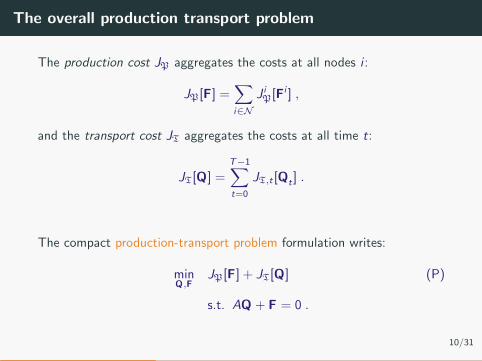
The overall production transport problem

The production cost JP aggregates the costs at all nodes i :

JP[F] =∑i∈N

J iP[Fi ] ,

and the transport cost JT aggregates the costs at all time t:

JT[Q] =T−1∑t=0

JT,t [Qt ] .

The compact production-transport problem formulation writes:

minQ,F

JP[F] + JT[Q] (P)

s.t. AQ + F = 0 .

10/31

Resolution methods

Where are we heading to?

The problem P has:

• N nodes (with N = 8);

• T time steps (with T = 12 or T = 52);

• N independent random variables per time step t: W1t , · · · ,WN

t .

We aim to solve the problem numerically. We suppose that for all t, Wit

is a discrete random variable, with support size nbin. Thus, the random

variable

Wt = (W1t , · · · ,W

Nt ) ,

has a support size nNbin (because of the independence).

11/31

First idea: solving the whole problem inplace!

Write the problem and solve it!

P

But ...

• N nodes and T time steps.

• Non-anticipativity constraint: we ought to formulate

the problem on a tree (Stochastic Programming approach)

number of nodes = (nNbin)T = nNTbin ,

giving a complexity in O(nNTbin ).

The problem is not tractable ...12/31

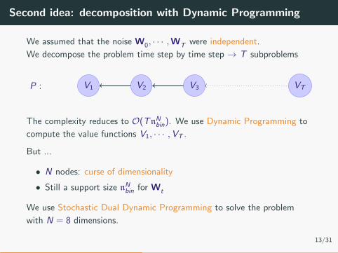
Second idea: decomposition with Dynamic Programming

We assumed that the noise W0, · · · ,WT were independent.

We decompose the problem time step by time step → T subproblems

P : V1 V2 V3 VT

The complexity reduces to O(TnNbin). We use Dynamic Programming to

compute the value functions V1, · · · ,VT .

But ...

• N nodes: curse of dimensionality

• Still a support size nNbin for Wt

We use Stochastic Dual Dynamic Programming to solve the problem

with N = 8 dimensions.

13/31

A brief recall on Stochastic Dynamic Programming

Dynamic Programming

We compute value functions with the backward equation:

VT (x) = K(x)

Vt(xt) = minut

E[Lt(xt , ut ,Wt+1)︸ ︷︷ ︸

current cost

+Vt+1

(f (xt , ut ,Wt+1)

)︸ ︷︷ ︸

future costs

]

Stochastic Dual Dynamic Programming

10 5 0 5 10x

0

20

40

60

80

100

y

• Convex value functions Vt are approximated as

a supremum of a finite set of affine functions

• Affine functions (=cuts) are computed during

forward/backward passes, till convergence

Vt(x) = max1≤k≤K

{λkt x + βk

t

}≤ Vt(x)

• SDDP makes an extensive use of LP/QP

solver 14/31

Third idea: spatial decomposition

We decompose the problem time by time and node by node to obtain

N × T decomposed subproblems:

P1 :

P2 :

...

PN :

V 11 V 1

2 V 13 V 1

T

V 21 V 2

2 V 23 V 2

T

V N1 V N

2 V N3 V N

T

λ11

λ2N1

λ1N1

λ122

λ2N2

λ123

λ2N3

The complexity reduces to O(NTnbin)! But ...

How to compute the different λ? 15/31

Introducing decomposition methods

The decomposition/coordination methods we want to deal with are

iterative algorithms involving the following ingredients.

• Decompose the global problem in several subproblems

of smaller size by dualizing the constraint AQ + F = 0,

• Coordinate at each iteration the subproblems using

the price λ.

AQ + F︸︷︷︸allocation

= 0 ; λ︸︷︷︸price

• Solve the subproblems using Dynamic Programming,

taking into account the price transmitted by the coordination.

16/31

Approximating the subproblems

In both cases, the subproblems encompass a new “noise”, that is,

the price multiplier λ(k)t , which may be correlated in time.

The white noise assumption fails.

Dynamic Programming cannot be used for solving the subproblems.

In order to overcome this difficulty, we use a trick that involves

approximating the new noise λkt by its conditional expectation w.r.t. a

chosen random variable Yt .

Assume that the process Y has a given dynamics:

Yt+1 = ht(Yt ,Wt+1) .

If noises Wt ’s are time independent, then (Xit ,Yt) is a valid state for the

i-th subproblem and Dynamic Programming applies.

17/31

Approximating the subproblems

In both cases, the subproblems encompass a new “noise”, that is,

the price multiplier λ(k)t , which may be correlated in time.

The white noise assumption fails.

Dynamic Programming cannot be used for solving the subproblems.

In order to overcome this difficulty, we use a trick that involves

approximating the new noise λkt by its conditional expectation w.r.t. a

chosen random variable Yt .

Assume that the process Y has a given dynamics:

Yt+1 = ht(Yt ,Wt+1) .

If noises Wt ’s are time independent, then (Xit ,Yt) is a valid state for the

i-th subproblem and Dynamic Programming applies.

17/31

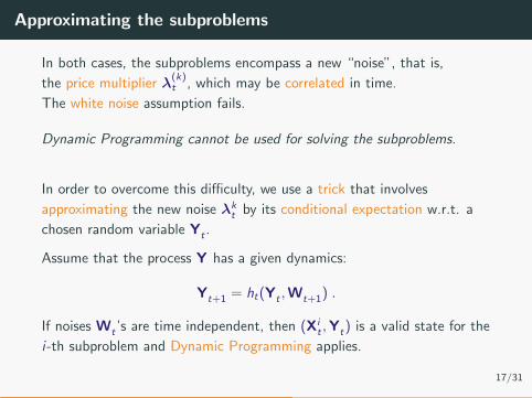
Approximating the subproblems

In both cases, the subproblems encompass a new “noise”, that is,

the price multiplier λ(k)t , which may be correlated in time.

The white noise assumption fails.

Dynamic Programming cannot be used for solving the subproblems.

In order to overcome this difficulty, we use a trick that involves

approximating the new noise λkt by its conditional expectation w.r.t. a

chosen random variable Yt .

Assume that the process Y has a given dynamics:

Yt+1 = ht(Yt ,Wt+1) .

If noises Wt ’s are time independent, then (Xit ,Yt) is a valid state for the

i-th subproblem and Dynamic Programming applies.

17/31

Price decomposition

The production and transport optimization problem writes

minQ,F

JP[F] + JT[Q] s.t. AQ + F = 0 .(P)

The decomposition scheme consists in dualizing the constraint, and then

in approximating the multiplier λ by its conditional expectation w.r.t. Y.

This trick leads to the following problem

maxλ

minQ,F

JP[F] + JT[Q] +⟨E(λ | Y) ,AQ + F

⟩.

It is not difficult to prove that this dual problem is associated

to the following relaxed primal problem:

minQ,F

JP[F] + JT[Q] s.t. E(AQ + F

∣∣ Y)

= 0 ,

and hence provides a lower bound of(P).

18/31

A dual gradient-like algorithm

Applying the Uzawa algorithm to the dual problem

maxλ

minQ,F

JP[F] + JT[Q] +⟨E(λ | Y) ,AQ + F

⟩,

leads to a decomposition between production and transport:

F(k+1) ∈ arg minF

JP[F] +⟨E(λ(k)

∣∣ Y),F⟩, Production

Q(k+1) ∈ arg minQ

JT[Q] +⟨E(λ(k)

∣∣ Y),AQ

⟩, Transport

E(λ(k+1)

∣∣ Y)

= E(λ(k)

∣∣ Y)

+ ρ E(AQ(k+1) + F(k+1)

∣∣ Y). Update

19/31

Decomposing the transport problem

The transport subproblem

minQ

JT[Q] +⟨E(λ(k)

∣∣ Y),AQ

⟩,

writes in a detailled manner

minQ

T−1∑t=0

E(∑

a∈Acat (Qa

t ) +⟨A>E

(λ

(k)t

∣∣ Yt

),Qt

⟩).

This minimization subproblem is evidently decomposable in time

(t by t) and in space (arc by arc), leading to a collection of easy

to solve subproblems.

20/31

Decomposing the production problem

The production subproblem

minF

JP[F] +⟨E(λ(k)

∣∣ Y),F⟩,

evidently decomposes node by node

minFi

J iP[Fi ] +⟨E(λi,(k)

∣∣ Y),Fi⟩,

hence a stochastic optimal control subproblem for each node i :

minXi ,Ui ,Fi

E( T−1∑

t=0

(Lit(Xi

t ,Uit ,F

it ,Wt+1) +

⟨E(λ

i,(k)t

∣∣ Yt

),Fi

t

⟩)+ K i (Xi

T )

)s.t. Xi

t+1 = f it (Xit ,U

it ,F

it ,Wt+1)

Uit � Ft .

21/31

Solving the production subproblems by DP

Assuming that

• the process W is a white noise,

• the process Y follows a dynamics Yt+1 = ht(Yt ,Wt+1),

Dynamic Programming applies for production subproblems:

V iT (x , y) = K i (x)

Vt(x , y) = minu,f

E(Lit(x , u, f ,Wt+1)

+⟨E(λi,(k)t

∣∣ Yt = y), f⟩

+ V it+1(Xi

t+1,Yt+1))

s.t. Xit+1 = f it (x , u, f ,Wt+1) ,

Yt+1 = ht(y ,Wt+1) .

22/31

Numerical implementation

Our stack is deeply rooted in Julia language

• Modeling Language: JuMP

• Open-source SDDP Solver:

StochDynamicProgramming.jl

• LP/QP Solver: Gurobi 7.02

https://github.com/JuliaOpt/StochDynamicProgramming.jl

23/31

Implementation of SDDP and DADP

• Implementing SDDP is straightforward

• DADP implementation is more elaborated:

E(λ(k+1)

∣∣ Y)

= E(λ(k)

∣∣ Y)

+ ρ E(AQ(k+1) + F(k+1)

∣∣ Y).

We use a crude relaxation:

• We choose Y = 0. We denote λ(k) = E(λ(k)

). The update becomes

λ(k+1) = λ(k) + ρ︸︷︷︸Update step

E(AQ(k+1) + F(k+1))︸ ︷︷ ︸

Monte Carlo

.

• Unfortunately, we do not know the Lipschitz constant of the

derivative!

• And the problem is not even strongly convex ...

24/31

We compare three algorithms for gradient ascent

• Quasi-Newton (BFGS): To ensure strong convexity, we add a quadratic term to the cost:

Lit(.) = Li

t(.) + u>Qu, with Q � 0. The update is:

λ(k+1) = λ

(k) + ρ(k) E

{AQ(k+1) + F(k+1)}

.

• Alternating Direction Method of Multipliers (ADMM): we add an augmented Lagrangian to

solve the problem. The update becomes

λ(k+1) = λ

(k) +τ

2E(AQ(k+1) + F(k+1))

.

• Stochastic Gradient Descent (SGD):

λ(k+1) = λ

(k) +1

1 + k

(AQ(k+1) + F(k+1))(ω) .

BFGS ADMM SGD

ρ line search ρ(k) → τ 1/(1 + k)

MC size 100-1000 100-1000 1

software L-BFGS-B3 self self

3The famous implementation of [Zhu et al, 1997]25/31

Double, double toil and trouble

Digesting the stochastic caldron, between time and space ...

BFGS ADMM SGD

DP

QP

• Global problem P

minQ,F

JP[F] + JT[Q]

s.t. AQ + F = 0 .

• Decomposed subproblem Pi

JP(Fi ) = minXi ,Ui ,Fi

E( T−1∑

t=0

(Lit (Xi

t , Uit , Fit , Wt+1)+

⟨E(λi,(k)t

∣∣ Yt), Fit

⟩)+ Ki (Xi

T )

)s.t. Xi

t+1 = f it (Xit , Ui

t , Fit , Wt+1)

• DP subproblem V it

V it (x, y) = min

u,fE(Lit (x, u, f , Wt+1)

+⟨E(λi,(k)t

∣∣ Yt = y), f⟩

+ V it+1(Xi

t+1, Yt+1))

26/31

Results — Monthly

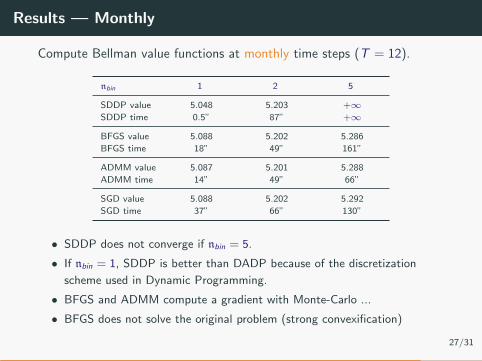
Compute Bellman value functions at monthly time steps (T = 12).

nbin 1 2 5

SDDP value 5.048 5.203 +∞SDDP time 0.5” 87” +∞

BFGS value 5.088 5.202 5.286

BFGS time 18” 49” 161”

ADMM value 5.087 5.201 5.288

ADMM time 14” 49” 66”

SGD value 5.088 5.202 5.292

SGD time 37” 66” 130”

• SDDP does not converge if nbin = 5.

• If nbin = 1, SDDP is better than DADP because of the discretization

scheme used in Dynamic Programming.

• BFGS and ADMM compute a gradient with Monte-Carlo ...

• BFGS does not solve the original problem (strong convexification)

27/31

Results — Weekly

Compute Bellman value functions at weekly time steps (T = 52).

nbin 1 2 5

SDDP value 9.396 9.687 +∞SDDP time 8” 928” +∞

BFGS value 9.411 9.687 9.974

BFGS time 69” 157” 575”

ADMM value 9.404 9.682 9.984

ADMM time 65” 326” 643”

SGD value 9.411 9.679 9.971

SGD time 194” 281” 712”

• The longer the horizon, the slower SDDP is.

• Here, BFGS is penalized by line-search, as it uses

an approximated gradient

• SGD works quite well compared to BFGS and ADMM: these two

algorithms are penalized by the Monte-Carlo computation of the gradient.

28/31

Multipliers convergence

0 10 20 30 40Iteration

0

250

500

750

1000

1250

1500

1750M

ultip

liers

Figure 1: Convergence of multipliers with BFGS (T = 12, nbin = 1).

29/31

SDDP convergence

0 20 40 60 80 100Iteration

0.88

0.90

0.92

0.94

0.96

0.98

1.00

1e8Lower boundUpper boundConfidence interval

Figure 2: Convergence of SDDP’s upper and lower bounds (T = 52, nbin = 2).

30/31

Conclusion

Conclusion

Conclusion

• A survey of different algorithms, mixing spatial

and time decomposition.

• DADP works well with the crude relaxation Y = 0,

and even beats SDDP if nbin ≥ 2.

• We had a lot of troubles to deal with approximate gradients!

Perspectives

• Find a proper information process Y.

• Improve the integration between SDDP and DADP.

• Test other decomposition schemes (by quantity, by prediction).

31/31

P. Carpentier et G. Cohen.

Decomposition-coordination en optimisation deterministe et stochastique.

En preparation, Springer, 2016.

P. Girardeau.

Resolution de grands problemes en optimisation stochastique dynamique.

These de doctorat, Universite Paris-Est, 2010.

V. Leclere.

Contributions aux methodes de decomposition en optimisation stochastique.

These de doctorat, Universite Paris-Est, 2014.

A. Lenoir and P. Mahey.

A survey of monotone operator splitting methods and decomposition of convex programs.

RAIRO Operations Research 51, 17-41, 2017.

Philippe Mahey, Jonas Koko, Arnaud Lenoir and Luc Marchand.

Coupling decomposition with dynamic programming for a stochastic spatial model for

long-term energy pricing problem.

31/31

Zhu, Ciyou and Byrd, Richard H and Lu, Peihuang and Nocedal,

Jorge.

L-BFGS-B: Fortran subroutines for large-scale bound-constrained optimization .

ACM Transactions on Mathematical Software (TOMS), 23-4, 1997.

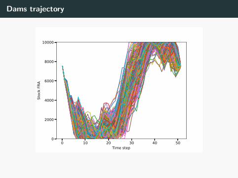
Dams trajectory

0 10 20 30 40 50Time step

0

2000

4000

6000

8000

10000St

ock

FRA

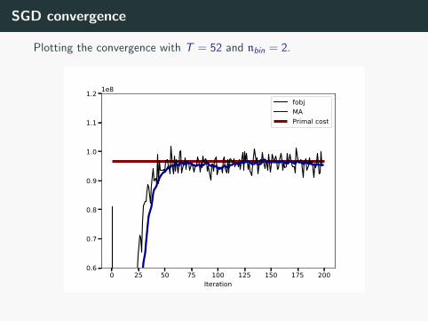
SGD convergence

Plotting the convergence with T = 52 and nbin = 2.

0 25 50 75 100 125 150 175 200Iteration

0.6

0.7

0.8

0.9

1.0

1.1

1.2 1e8fobjMAPrimal cost

ADMM convergence

Plotting the logarithm of the norm of the primal residual with T = 52

and nbin = 5.

0 10 20 30 40 50 60Iteration

1.0

1.5

2.0

2.5

3.0

log(

||g||)