optimization in control applications
TRANSCRIPT

Optimization in Control Applications
Guillermo Valencia-Palomo and Francisco Ronay López-Estrada
www.mdpi.com/journal/mca
Edited by
Printed Edition of the Special Issue Published in Mathematical and Computational Applications
Mathematical and Computational Applications

Optimization in Control Applications


Optimization in Control Applications
Special Issue Editors
Guillermo Valencia-Palomo
Francisco Ronay Lopez-Estrada
MDPI • Basel • Beijing • Wuhan • Barcelona • Belgrade

Special Issue Editors
Guillermo Valencia-Palomo
Instituto Tecnologico de
Hermosillo
Mexico
Francisco Ronay Lopez-Estrada
Instituto Tecnologico de Tuxtla
Gutierrez
Mexico
Editorial Office
MDPI
St. Alban-Anlage 66
4052 Basel, Switzerland
This is a reprint of articles from the Special Issue published online in the open access journal
Mathematical and Computational Applications (ISSN 2297-8747) in 2018 (available at: https://www.
mdpi.com/journal/mca/special issues/optimization in control)
For citation purposes, cite each article independently as indicated on the article page online and as
indicated below:
LastName, A.A.; LastName, B.B.; LastName, C.C. Article Title. Journal Name Year, Article Number,
Page Range.
ISBN 978-3-03897-447-5 (Pbk)
ISBN 978-3-03897-448-2 (PDF)
c© 2018 by the authors. Articles in this book are Open Access and distributed under the Creative
Commons Attribution (CC BY) license, which allows users to download, copy and build upon
published articles, as long as the author and publisher are properly credited, which ensures maximum
dissemination and a wider impact of our publications.
The book as a whole is distributed by MDPI under the terms and conditions of the Creative Commons
license CC BY-NC-ND.

Contents
About the Special Issue Editors . . . . . . . . . . . . . . . . . . . . . . . . . . . . . . . . . . . . . vii
Preface to ”Optimization in Control Applications” . . . . . . . . . . . . . . . . . . . . . . . . . . ix
Chahid Kamel Ghaddar
Rapid Solution of Optimal Control Problems by a Functional Spreadsheet Paradigm: A PracticalMethod for the Non-ProgrammerReprinted from: Math. Comput. Appl. 2018, 23, 54, doi:10.3390/mca23040054 . . . . . . . . . . . . 1
Chahid Kamel Ghaddar
Novel Spreadsheet Direct Method for Optimal Control ProblemsReprinted from: Math. Comput. Appl. 2018, 23, 6, doi:10.3390/mca23010006 . . . . . . . . . . . . . 29
Imane Abouelkheir, Fadwa El Kihal, Mostafa Rachik and Ilias Elmouki
Time Needed to Control an Epidemic with Restricted Resources in SIR Model with Short-TermControlled Population: A Fixed Point Method for a Free Isoperimetric Optimal Control ProblemReprinted from: Math. Comput. Appl. 2018, 23, 64, doi:10.3390/mca23040064 . . . . . . . . . . . . 52
Ellina Grigorieva and Evgenii Khailov
Optimal Strategies for Psoriasis TreatmentReprinted from: Math. Comput. Appl. 2018, 23, 45, doi:10.3390/mca23030045 . . . . . . . . . . . . 70
Segun Isaac Oke, Maba Boniface Matadi and Sibusiso Southwell Xulu
Optimal Control Analysis of a Mathematical Model for Breast CancerReprinted from: Math. Comput. Appl. 2018, 23, 21, doi:10.3390/mca23020021 . . . . . . . . . . . . 100
Dibyendu Biswas, Suman Dolai, Jahangir Chowdhury, Priti K. Roy and Ellina V. Grigorieva
Cost-Effective Analysis of Control Strategies to Reduce the Prevalence of CutaneousLeishmaniasis, Based on a Mathematical ModelReprinted from: Math. Comput. Appl. 2018, 23, 38, doi:10.3390/mca23030038 . . . . . . . . . . . . 128
Fadwa El Kihal, Imane Abouelkheir, Mostafa Rachik and Ilias Elmouki
Optimal Control and Computational Method for the Resolution of Isoperimetric Problem in aDiscrete-Time SIRS SystemReprinted from: Math. Comput. Appl. 2018, 23, 52, doi:10.3390/mca23040052 . . . . . . . . . . . . 157
Johanna Pyy, Anssi Ahtikoski, Alexander Lapin and Erkki Laitinen
Solution of Optimal Harvesting Problem by Finite Difference Approximations ofSize-Structured Population ModelReprinted from: Math. Comput. Appl. 2018, 23, 22, doi:10.3390/mca23020022 . . . . . . . . . . . . 171
Raheleh Jafari and Sina Razvarz
Solution of Fuzzy Differential Equations Using Fuzzy Sumudu TransformsReprinted from: Math. Comput. Appl. 2018, 23, 5, doi:10.3390/mca23010005 . . . . . . . . . . . . . 186
Lizeth Torres, Javier Jimenez-Cabas, Jose Francisco Gomez-Aguilar and Pablo Perez-Alcazar
A Simple Spectral ObserverReprinted from: Math. Comput. Appl. 2018, 23, 23, doi:10.3390/mca23020023 . . . . . . . . . . . . 201
v

Sasitorn Kaewman, Tassin Srivarapongse, Chalermchat Theeraviriya and
Ganokgarn Jirasirilerd
Differential Evolution Algorithm for Multilevel Assignment Problem: A Case Study in ChickenTransportationReprinted from: Math. Comput. Appl. 2018, 23, 55, doi:10.3390/mca23040055 . . . . . . . . . . . . 215
Jose-Roberto Bermudez, Francisco-Ronay Lopez-Estrada, Gildas Besancon, Guillermo
Valencia-Palomo, Lizeth Torres, Hector-Ricardo Hernandez
Modeling and Simulation of a Hydraulic Network for Leak DiagnosisReprinted from: Math. Comput. Appl. 2018, 23, 70, doi:10.3390/mca23040070 . . . . . . . . . . . . 234
vi

About the Special Issue Editors
Guillermo Valencia-Palomo was born in Merida, Yucatan, Mexico, in 1980. He received an
Engineering degree in Electronics from the Instituto Tecnologico de Merida, Mexico, in 2003;
an M.Sc. in Automatic Control from the National Center of Research and Technological Development
(CENIDET), Mexico, in 2006; and a Ph.D. degree in Automatic Control and Systems Engineering
from The University of Sheffield, U.K., in 2010. Since 2010, Dr. Guillermo Valencia-Palomo has
been a full-time professor at Tecnologico Nacional de Mexico/Instituto Tecnologico de Hermosillo
(Mexico). He is the author/co-author of more than 80 research papers published in ISI-Journals and
international conferences. As a product of his research, he has one patent in commercial exploitation.
He has led a number of funded research projects, and these grants’ income represents a mixture of
sole investigator funding, collaborative grants, and funding from industry. His research interests
include predictive control, descriptor systems, linear parameter varying systems, fault detection,
fault tolerant control systems, and their applications to different physical systems.
Francisco-Ronay Lopez-Estrada received his Ph.D. in Automatic Control from the University of
Lorraine, France, in 2014. He has been with Tecnologico Nacional de Mexico/Instituto Tecnologico
de Tuxtla Gutierrez, Mexico, as a lecturer since 2008. He received his M.Sc. degree in Electronic
Engineering in 2008 from the National Center of Research and Technological Development
(CENIDET), Mexico. He has led several funded research projects. His research interests are descriptor
systems, TS systems, fault detection, fault-tolerant control, and their applications to unmanned
vehicles and pipeline leak detection systems.
vii


Preface to ”Optimization in Control Applications”
Mathematical optimization is the selection of the best element in a set with respect to a
given criterion. Optimization has become one of the most used tools in modern control theory
for computing the control law, adjusting the controller parameters (tuning), model fitting, finding
suitable conditions in order to fulfill a given closed-loop property, etc. In the simplest case,
optimization consists of maximizing or minimizing a function by systematically choosing input
values from a valid input set and computing the function value. To solve optimization problems,
researchers can use algorithms that end in a finite number of steps, or iterative methods that converge
to a solution (in some specific class of problems), or heuristics that can provide approximate solutions
to some problems (although their iterations do not necessarily converge). In practice, real-world
control systems need to comply with several conditions and physical and product-quality constraints
that have to be taken into account in the problem formulation. These represent challenges in the
application/implementation of the optimization algorithms, particularly when the solutions of these
optimization problems have to be computed in a constrained time window and/or in an embedded
platform.
This Special Issue provides a forum for high-quality peer-reviewed papers that broaden the
awareness and understanding of advanced optimization techniques and their applications in control
engineering. This topic encompasses many algorithms and process flows and tools, including:
optimal control of nonlinear systems; optimal control of complex systems; optimal observer design;
numerical optimization; evolutionary optimization; and constrained optimization; among others.
Specifically, this Special Issue gathers twelve papers that contribute to this topic by presenting: rapid
solutions of optimal control problems by a functional spreadsheet paradigm; a novel spreadsheet
direct method for optimal control problems; a fixed point method for a free isoperimetric optimal
control problem to control an epidemic with restricted resources in an SIR model with a short-term
controller population; optimal strategies for psoriasis treatment; an optimal control analysis of a
mathematical model for breast cancer; a cost-effective analysis of control strategies to reduce the
prevalence of cutaneous leishmaniasis based on a mathematical model; an optimal control and
computation method for the solution of an isoperimetric problem in a discrete-time SIRS system;
a solution of an optimal harvesting problem by finite difference approximations of a size-structured
population model; a solution of fuzzy differential equations using fuzzy Summudu transformations;
the development of a spectral observer for the reconstruction of a time signal via state estimation and
its frequencies decomposition; a differential evolution algorithm for a multilevel assignment problem;
and the modelling and simulation of a hydraulic network for leak diagnosis and optimal control.
We believe that the papers in this Special Issue reveal an exciting area which can be expected
to continue to grow in the very near future—namely, the use of advanced optimization strategies in
engineering applications. The pursuit of work in this area requires expertise in control engineering
as well as in systems design and numerical analysis. We hope that this issue helps to bring these
communities into closer contact with each other, as the fruitfulness of collaboration across these areas
becomes clear.
Guillermo Valencia-Palomo, Francisco Ronay Lopez-Estrada
Special Issue Editors
ix


Mathematical
and Computational
Applications
Article
Rapid Solution of Optimal Control Problems by aFunctional Spreadsheet Paradigm: A PracticalMethod for the Non-Programmer
Chahid Kamel Ghaddar
ExcelWorks LLC, Sharon, MA 02067, USA; [email protected]; Tel.: +1-781-626-0375
Received: 29 August 2018; Accepted: 26 September 2018; Published: 28 September 2018
Abstract: We devise a practical and systematic spreadsheet solution paradigm for general optimalcontrol problems. The paradigm is based on an adaptation of a partial-parametrization direct solutionmethod which preserves the original mathematical optimization statement, but transforms it into asimplified nonlinear programming problem (NLP) suitable for Excel NLP solver. A rapid solutionstrategy is implemented by a tiered arrangement of pure elementary calculus functions in conjunctionwith Excel NLP solver. With the aid of the calculus functions, a cost index and constraints arerepresented by equivalent formulas that fully encapsulate an underlining parametrized dynamicalsystem. Excel NLP solver is then employed to minimize (or maximize) the cost index formula,by varying decision parameters, subject to the constraints formulas. The paradigm is demonstratedfor several fixed and free-time nonlinear optimal control problems involving integral and implicitdynamic constraints with direct comparison to published results obtained by fundamentally differentmethods. Practically, applying the paradigm involves no more than defining a few formulas usingbasic Excel spreadsheet skills.
Keywords: optimal control; dynamic optimization; mathematical programming; differentialequations; parameter estimation; Excel spreadsheet; calculus functions
1. Introduction
Many researchers and academics often need to solve optimal control problems that are frequentlypostulated in various engineering, social, and life sciences [1–3]. An optimal control problem isconcerned with finding control functions, (or policies), that achieve optimal trajectories for a set ofcontrolled differential state variables. The optimal trajectories are determined by solving a constraineddynamical optimization problem, such that a cost index is minimized (or maximized), subject toconstraints on state variables and control functions. Mathematically, an optimal control problem maybe stated generally as follows (bold symbols indicate vector-valued functions):
Find control functions u(t) = (u1(t), u2(t), . . . , um(t)) and corresponding state variablesx(t) = (x1(t), x2(t), . . . , xn(t)), t ∈ [t0, tF] which minimize (or maximize) the cost index
J = H(x(T), T) +∫ tF
t0
G(x(t),.x(t),
..x(t), u(t),
.u(t), t) dt, (1)
subject to
Mdxdt
= F(x(t), u(t), t), (2)
with initial conditionsx(0) = x0, (3)
Math. Comput. Appl. 2018, 23, 54; doi:10.3390/mca23040054 www.mdpi.com/journal/mca1

Math. Comput. Appl. 2018, 23, 54
and end conditions and boundsQ(x(T), T) = 0, (4)
S(x(t), u(t),
.x(t),
.u(t)
) ≤ 0. (5)
In the formulation (1)–(5), the generally nonlinear H, and G are scalar functions, whereas F, Q andS are vector valued functions. Typically, either H or Q are specified but not both in the same problem.Common forms of Q and S are end conditions on the state variables, x(T) = xT , and bound constraintson the controls, umin ≤ u(t) ≤ umax respectively. More general forms of S considered in this paperinclude algebraic and integral constraints involving derivatives. The matrix M in (2) offers an optionalcoupling of states’ temporal derivatives by a mass matrix which may be singular. If M is singular,the equation system (2) is differential algebraic, or DAE. For uncoupled derivatives, M is the identitymatrix which can be omitted. Furthermore, tF, which denotes the final time, may be fixed or free.
Numerical solution strategies for (1)–(5) can be classified into two approaches: indirect and directmethods. Indirect methods employ Pontryagin’s minimum principle to transform the problem into anaugmented Hamiltonian system requiring the solution of a boundary value problem which may behard to solve [4,5]. On the other hand, direct method approaches transform the original optimal controlproblem into a nonlinear programming problem which can be solved by various established NLPpackages. The transformation is carried out via a discretization of the control and the state functionson a time grid using some form of a collocation method [4,6,7]. Complete discretization of the stateand control functions eliminate the need to iteratively solve the inner initial value problem (IVP) (2) butat the expense of a large numbers of decision variables for the NLP solver. Other direct approachesrely only on a partial parametrization for the control functions using piecewise constant or higherorder polynomial approximations [8]. In this approach, the inner IVP must be solved repeatedly bythe outer NLP algorithm while searching for the optimal parameter vector. Except for the most trivialcases, optimal control problems are inherently nontrivial to solve. They typically require a level ofprogramming fluency, in addition to a good understanding of the general structure of the solutionstrategy, and the various solvers required to implement it [9].
In [10], the author introduced a practical spreadsheet method for solving a class of optimal controlproblems using basic spreadsheet skills. The method utilized two elementary calculus functions: aninitial value problem solver and a discrete data integrator from an available Excel calculus Add-in [11]in conjunction with Excel intrinsic NLP solver to formulate a partial-parametrization direct solutionstrategy. With the aid of the calculus functions, a cost index was represented by an equivalentformula that fully encapsulated a control-parametrized inner IVP (2)–(3). Excel NLP solver wasemployed next for minimizing (or maximizing) the cost index formula, by varying a decision parametervector, subject to bounds constraints on state and control variables. The method proved effective atsolving several nonlinear optimal control problems reproduced from Elnagar and Kazemi [6] whoemployed a full-parametrization direct method using pseudo-spectral approximation and NLPQLoptimization software.
This research paper aims at generalizing the method introduced in [10] for more generalformulations of optimal control than previously considered. More specifically, this paper demonstratesa systematic solution strategy formulated by the aid of various elementary calculus functions,for optimal control problems involving one or more of the following conditions: dependence onhigher order derivatives of state or control variables in the cost index and constraints; integral andalgebraic dynamic constraints; as well as implicit inner IVP. In addition, this paper investigatesconvergence and error control of the method, and provides direct comparison of optimal trajectorieswith published solutions obtained by fundamentally different methods.
It should be noted that the solution strategy formulation pursued in this research, althoughfounded on a common approach, follows closely the original mathematical problem statement,and thus implementation of the strategy varies according to the given problem. Therefore, the papergives considerable emphasis on the application of the method using four representative problems
2

Math. Comput. Appl. 2018, 23, 54
selected from various applications. Results presented in Section 3 are remarkable, in terms ofconvergence, agreement with published solutions, and notably, the minimal effort required to obtainthem with basic spreadsheet formulas.
In view of traditional spreadsheet applications, the devised solution strategy represents a leapin the utilization of the spreadsheet for solving general optimal control problems. The strategydeparts markedly from prior spreadsheet approaches [12,13] by shifting the effort from a low-leveldetailed algorithmic implementation to a high-level problem modeling. Prior approaches utilizedthe spreadsheet explicitly as the computational grid for the discretization and solution of the innerIVP. This effectively constrained the scope to rather simple problems that can be easily discretizedwith an explicit differencing scheme suitable for the spreadsheet. In contrast, we employ a set ofpure calculus functions for computing integrals, derivatives and solving differential equations as thebuilding blocks for a direct solution method. The calculus functions, described in Appendix A, utilizeadaptive algorithms which are independent of the spreadsheet grid and thus suitable for a generalclass for nonlinear stiff problems. The calculus functions are utilized in formulas just like intrinsicmath functions based on a simple input/output model. In essence, the calculus functions representa natural extension of the built-in spreadsheet math functions with the allowance that some of theirinput arguments are functions themselves and not just static values.
The reminder of this paper is organized as follows: In the next section, we present an outline ofthe general steps required to implement the direct spreadsheet solution strategy, and discuss sources oferrors that impact convergence and accuracy of the solution as well as possible remedies. In Section 3,we apply the method for solving four different optimal control problems selected to demonstratethe various conditions outlined earlier. Direct comparisons of optimal trajectories obtained by themethod versus published solutions obtained by fundamentally different approaches are also provided.In addition, effects of parametrization order and error control are investigated in some problems.Section 4 presents concluding remarks as well as directions for future research. Detailed descriptionsof the various calculus functions utilized in this work are included in Appendix A.
2. Mechanics of Spreadsheet Direct Method
The solution strategy is based on an adaptation of the control-parametrization direct approach [4,8]by an analogous spreadsheet functional formulation. The building blocks of the functional formulationare a set of calculus spreadsheet functions [11,14] which integrate with the spreadsheet, like intrinsicpure math functions, but also accept formulas as a new type of argument for solving problems inintegral, algebraic, and differential calculus. For example, an integration function accepts a formulaand limits as inputs, and it outputs an accurate integral value much like an intrinsic math functionaccepts a number and computes its square root. Specifically, we make use of the following functionsfrom a calculus Add-in [11]:
• Initial value problem solver, IVSOLVE, using RADAU5 an implicit 5th-order Runge-Kuttaalgorithm with adaptive time step [15].
• Discrete data Integrator, QUADXY, using cubic splines [16].• Discrete data differentiator, DERIVXY, using cubic splines [16].• Formula integrator, QUADF, using Gauss quadrature with adaptive error control [17].
The functions are utilized in combination with Excel NLP solver, which is based on the GeneralizedReduced Gradient algorithm based on Lasdon and Waren [18]. A detailed description of the calculusfunctions usage, and respective algorithms are given in Appendix A. The critical characteristic ofthe calculus functions which permits their seamless utilization with the NLP solver in a functionalparadigm, is the mathematical purity property. The calculus functions do not modify their inputs,and produce no side effects in the spreadsheet. They only compute and display a solution result intheir allocated spreadsheet memory cells. The authority to modify the inputs to the calculus functions,via changes to the decision parameter vector, is confined to the outer NLP solver command.
3

Math. Comput. Appl. 2018, 23, 54
Below, we describe the main elements of the solution strategy introduced originally in [10] butgeneralized in this work for solving general optimal control problem (1)–(5) with the aim of supportingthe various conditions outlined earlier.
2.1. Solution Strategy
The strategy comprises three ordered steps which are implemented by the aid of calculus functions:In the first step, we obtain an initial solution to the inner IVP (2)–(3), based on suitable
parametrization for the control functions with initial guesses for the unknown parameters and afinal time for free-time problems. The unknown parameters and the final time constitute the decisionvariables for the final optimization step by the outer NLP solver. Any prior information about thecontrols should be incorporated in the specified parametrization. Absent any information, a low-orderpolynomial is often an adequate choice. The initial IVP solution is obtained by the calculus functionIVSOLVE which displays the state variables, x(t), in an allocated array of the spreadsheet at uniformoutput time points. It should be noted that output time grid is determined by the number of rowsin the allocated output array but is, otherwise, unrelated to the accuracy of the computed solution.To display a finer output time grid, a larger output array should be allocated. However, the resolutionof the output time grid affects the accuracy of the computed integrals for the cost index and anyintegral constraints which is discussed in Section 2.2. Optional parameters to IVSOLVE could also beused to control or specify the output time points.
In the second step, we construct an analogous formula for the cost index (1) dependent onthe initial solution outputted by IVSOLVE. The cost index may depend on x(t), the control values,u(t), as well as first and higher order derivatives of the state variables and controls. Values for u(t),.u(t) and higher derivatives are readily generated using the specified parametrized formula for acontrol u(t). The spreadsheet is particularly suited for such computations using its AutoFill feature.On the other hand, values for the state variables derivatives
.x(t), and
..x(t) are not readily available
and must be approximated by differentiating x(t) values obtained by IVSOLVE. We accomplishthis task by the aid of a discrete data differentiator calculus function DERIVXY which computesderivatives using cubic splines to model the best function described by x(t). With all the necessaryvalues obtained, we proceed to defining an analogous formula for the cost index, which is typicallydefined as a continuous time integral of an algebraic integrand. The devised method is to sample theintegrand expression using the obtained values for the states, controls and their derivatives, followedby employing a discrete data integrator calculus function QUADXY to integrate a cubic-spline fitfunction through the sampled integrand. Depending on a particular problem formulation, it may benecessary to define additional formulas to represent constraints equations (5) that may be present.Such formulas can often be constructed in a similar way to the cost index formula using appropriatecalculus functions. In particular, we shall demonstrate in Section 3 using an additional formulaintegrator function QUADF to define an integral constraint formula.
Figure 1 illustrates the aforementioned steps applied to an optimal control problem with onecontrol and two state variables. An initial IVP solution, which is dependent on a decision parametersvector, is obtained with IVSOLVE in an array (Figure 1a). Values for the control, u(t), and anyneeded state derivatives such as
..x1(t), are generated in additional columns (Figure 1b,c) at the time
values of the IVP solution. Next, the cost index integrand expression is sampled at the IVP solutiontimes (Figure 1d), and the sample is then integrated to define the cost index formula (Figure 1e).The generated values interdependence hierarchy ensures that any change to the decision parametersvector, such as by an outer NLP solver, will trigger reevaluation of the cost index formula in the properorder shown in the figure. The cost index formula thus fully encapsulates the inner IVP problem.
In the last step, we configure Excel NLP solver to minimize (or maximize) the cost index formulaby varying the decision parameters vector subject to bounds, end conditions and other presentconstraints. Bound constraints on x(t), as well as end point constraints on x(T), are imposed directlyon the corresponding values in the IVP solution array. More general constraints are imposed on
4

Math. Comput. Appl. 2018, 23, 54
additional formulas constructed in step 2 as needed. The three steps are demonstrated on severalexamples in the next section.
A B C D E F G H I1 t X1 X2 u(t) X1’’(t) Integrand(t) Cost Index2 0 # # # # # #3 0.05 # # # # #4 0.1 # # # # #100 4.9 # # # # #101 4.95 # # # # #102 5 # # # # #
(a)IVP solution array obtained with IVSOLVE
(b)Control valuesgenerated fromparameterizedformula
(c)generated
using DERIVXY
(d)Cost integrandsampled usingcolumns A to F
(e)
Cost index formula
defined by integrating
(e) using QUADXY
Figure 1. Illustration of the ordered steps to define an analog formula for the cost index (1) whichencapsulates the inner IVP (2)–(3).
2.2. Convergence and Error Control
Two sources of errors are introduced by the spreadsheet method with respect to the originalproblem. The first error is introduced by restricting the space of admissible control functions to afinite-dimensional space, for example, variable-order polynomials up to a fixed degree. For someproblems, it may not be possible to find a solution if the optimal control, in fact, lies outside theadmissible space. The second source of error is introduced by the calculus numerical algorithms.This error can be further split into two sources. The error associated with solution of the inner IVP,and the error associated with integration (or differentiation) of discrete data sets generated from theIVP solution. The first error is bounded by the tolerances specified for IVSOLVE algorithm. The seconderror impacts the accuracy of the computed integral for the cost index. Under the assumption thatthe discrete data describe a smooth curve, the computed integral by QUADXY using cubic splines isgenerally quite accurate. However, it may be further improved by any of the following acts.
• Increasing the size of the data set by increasing the number of rows of the allocated IVP solutionarray to output a finer time grid.
• Supplying optional slopes at the end points of the curve to the calculus function when available.The slopes may be derived analytically from the integrand expression and can improve theaccuracy of the spline fit near the curve edges.
• Using nonuniform output time points clustered near rapidly-varying regions of the statetrajectories. This can be controlled via optional arguments to IVSOLVE including supplyingexact values for the output time points.
In practice, we have found that the parametrization order and the starting guess for unknownparameters to be the most important factors influencing convergence. We have generally usedpolynomials up to 5th order which have performed reasonably well. On the other hand, increasingthe output array for IVP solution beyond a reasonable size, on the order of 100 uniform subdivisionsfor the time interval, has not generally resulted in a consistent or significant improvement of theresult. In the examples in the next section, we shall demonstrate the effects of both increasing theparametrization order and reducing the output time interval.
5

Math. Comput. Appl. 2018, 23, 54
3. Illustrative Optimal Control Problems
In the following subsections we apply the method to four different optimal control problemsrepresenting various engineering applications and compare the optimal trajectories with publishedsolutions. The computations were carried out on a standard laptop computer with an Intel i7 four-coreprocessor at 2.70 GHz running Microsoft Windows 10 and Excel 2016 with ExceLab calculus add-in [11],which enables the calculus function in Excel. A supplementary Excel workbook containing the solvedexamples is available for downloading from the publisher.
3.1. Minimum Energy Shape: Hanging Chain
The first example is concerned with finding the shape u(t) of a chain of length L suspendedbetween two points, such that its total energy is minimized. We state the problem as described in [19]with L = 4, below:
Find u(t) which minimizes the total energy cost index
J =∫ 1
0u(t)
√1 +
.u(t)2dt, (6)
subject to the chain length constraint
∫ 1
0
√1 +
.u(t)2dt = 4, (7)
and the end conditionsu(0) = 1, (8)
u(1) = 3. (9)
Note that in this problem formulation, the inner IVP is implicitly defined by the integralconstraint (7). Dolan et al. [19] reformulated the problem, via variable substitution, as a standardoptimal control problem subject to a system of explicit differential equations and solved it by adirect approach. Discretization was done using a uniform time step and the trapezoidal rule for theintegration. Results for the AMPL implementation were reported using several solvers includingKNITRO and LOQO. The best cost index was found at 5.06852 starting from a quadratic approximationand using a grid of 800 nodes. Our spreadsheet solution below is formulated based on the originalproblem statement (6)–(9).
3.1.1. Solution by Direct Spreadsheet Method
Referring to Figure 2, we setup problem (6)–(9) in Excel using named variables with labels listedin column A. The shape function u(t) was parametrized using a 3rd order polynomial with unknowncoefficients c_0, c_1, c_2 and c_3 as shown by formula B7. In B15 and B16, formulas for the initial andfinal values, u(0) and u(1) were defined by evaluating B7 at time equal zero and one (these formulas areused later to impose the constraints (8)–(9)). An additional formula was defined in B8, (named udot),for the shape function derivative,
.u(t) by differentiating B7 with respect to time. Next, we defined the
cost index integral (6), by using the integration calculus function QUADF as shown in B11. The first
parameter to QUADF is the integrand u(t)√
1 +.u(t)2 which is defined by the equivalent formula
in B10. The 2nd parameter is the variable of integration t, and the 3rd and 4th parameters are theintegration limits. Likewise, with the aid of QUADF, we defined the constraint integral (7) as shown inB14 (named I_c). This completed the model needed to run Excel NLP solver.
3.1.2. Results and Analysis
Excel NLP solver is invoked from the Data tab on Excel Ribbon and displays a dialog to enterthe problem objective, variables and constraints. Figure 3 shows the inputs for problem 3.1 in which
6

Math. Comput. Appl. 2018, 23, 54
the objective J (B11), was selected to be minimized, by varying the parameters c_0, c_1, c_2 and c_3,subject to the three constraints: I_c = 4, corresponding to (7); u_0 = 1, corresponding to (8); and u_1 = 3,corresponding to (9).
A B 1 t 2 Parametrized chain shape function 3 c_0 0 4 c_1 0 5 c_2 0 6 c_3 0 7 u =c_0+c_1*t+c_2*t^2+c_3*t^3 8 udot =c_1+2*c_2*t+3*c_3*t^2 9 Cost Index
10 =u*(SQRT(1+udot^2)) 11 J =QUADF(B10,t,0,1) 12 Constraints definitions 13 =SQRT(1+udot^2) 14 I_c =QUADF(B13,t,0,1) 15 u_0 =c_0 16 u_1 =c_0+c_1+c_2+c_3
Figure 2. Spreadsheet parametrized model for problem 3.1.
Figure 3. Input to Excel solver for problem 3.1 based on the spreadsheet model in Figure 2.
7

Math. Comput. Appl. 2018, 23, 54
The solver converged, starting from a zero guess for the parameters in less than a second to theresult shown in Figure 4 with a final cost index of 5.0751. The optimal shape function u(t) is plotted inFigure 5 together with digitally-read values from the plot published in [19].
Figure 4. Answer report generated by Excel solver using 3rd order parametrization for problem 3.1.
Figure 5. Optimal u(t) computed using 3rd order parametrization for problem 3.1. Reported values byDolan et al. are also shown.
8

Math. Comput. Appl. 2018, 23, 54
The difference between the value reported by Dolan et al. [19] and our computed value using acubic approximation for u(t) is approximately 0.13%. We have tried a quadratic approximation andobtained a slightly higher cost index of 5.078412. It is likely that the small difference originated fromintegration error in [19] using a trapezoidal rule, whereas the integration in our solution by QUADFcalculus function is based on an adaptive Gauss-quadrature scheme [17] which is accurate to machineprecision for a smooth polynomial integrand.
To demonstrate the effect of control parametrization order on the result, next we tried a 5th-orderpolynomial approximation to the shape function u(t), but also appended the problem with oneadditional constraint:
u(t) ≥ 0. (10)
Incorporating (10) into the spreadsheet model was accomplished as follows. In a new column, a vectorof time values from 0 to 1 in increment of 0.1 was generated using Excel AutoFill feature, along with acorresponding vector for the parametrized shape formula as shown in Figure 6. To impose (10), it issufficient to demand that the minimum value of the shape vector, as computed in F13 of Figure 6,be greater than or equal to zero. Running the NLP solver with the added constraint yielded a costindex of 4.654 as shown in Figure 7 and plotted in Figure 8. The higher-order approximation to theshape function has resulted in a considerably lower cost index, by more than 8.3%, compared to thatreported by Dolan et al. [19].
E F 1 t u(t) 2 0 1 3 0.1 1.11111 4 0.2 1.24992 5 0.3 1.42753 6 0.4 1.65984 7 0.5 1.96875 8 0.6 2.38336 9 0.7 2.94117
10 0.8 3.68928 11 0.9 4.68559 12 1 6 13 min(u) 1
=c_0+c_1*E2+c_2*E2^2+c_3*E2^3+c_4*E2^4+c_5*E2^5
=MINA(F2:F12)
Figure 6. Parametrized u(t) function is sampled with AutoFill to provide a handle on its minimumvalue for the purpose of imposing constraint (10).
9

Math. Comput. Appl. 2018, 23, 54
Figure 7. Answer report generated by Excel solver using a 5th order parametrization for problem 3.1with the added constrained (10).
Figure 8. Optimal u(t) computed by using 5th order parametrization for problem 3.1. The higher-costsolution with 3rd order parametrization and reported values by Dolan et al. are also shown.
3.2. Quadratic Control Problem with Integral Constraint
The following problem which involves an integral dynamic constraint was studied byLim et al. [20], who showed the that the optimal control can be calculated by solving an optimal
10

Math. Comput. Appl. 2018, 23, 54
parameter selection problem together with an unconstrained LQ problem. The optimal controlproblem is stated as follows:
Find u1(t), u2(t), t ∈ [0, 1] which minimize the cost index
J = 0.5 x1(1)2 + 0.5
∫ 1
0
(x1
2 + u12 + u2
2)
dt, (11)
subject to.x1 = 3x1 + x2 + u1, (12)
.x2 = −x1 + 2x2 + u2, (13)
with initial conditionsx1(0) = 4, x2(0) = −4, (14)
and integral bounds constraint (There appears to be a typographical error in [20] where (15) is statedas less than 8. The actual value appears to be 80 since 8 would clearly violate the constraint at thereported optimal solution in [20].)
0.5 x2(1)2 + 0.5
∫ 1
0
(x1
2 + u12 + u2
2)
dt ≤ 80. (15)
Lim et al. [20] calculated, with aid of control software MISER 3.1, an optimal cost index J of 62.66103.
3.2.1. Solution by Direct Spreadsheet Method
Referring to Figure 9 and working with named variables shown in column A, both u1(t) and u2(t)were parametrized using 3rd-order polynomials as shown in B10 and B11, and the IVP equations (12)and (13) were defined by equivalent formulas in B13 and B14. The state variables x1 and x2 are assignedthe initial conditions as shown in B3 and B4. Next, an initial solution to the underlining IVP (12)–(14)was obtained by evaluating the formula
=IVSOLVE(B13:B14, B2:B4, {0,1}) (16)
in an allocated array E1:G102. IVSOLVE was passed the IVP equations B13:B14, the IVP variables B2:B4,and the time interval [0, 1] and computed a formatted result shown partially in Figure 10. Here wehave allocated 102 rows for the result array to display the solution at uniform time steps of 0.01.
To define an equivalent formula for the cost index (11), we proceeded by sampling the controlsformulas, and the cost index integrand as shown in columns I, J and K of Figure 10 by starting from theinitial formulas shown in the figure and using AutoFill to generate the values. (Note the hierarchicalinterdependence of the generated columns on the IVP solution). Next, we defined the cost indexformula in which the discrete data integrator calculus function QUADXY was employed to integratethe sampled integrand as shown in B16 of Figure 9. Similarly, we defined an analog formula for theintegral constraint (15) as shown in B18 of Figure 9, and thus prepared all the input needed to runExcel NLP solver next.
11

Math. Comput. Appl. 2018, 23, 54
A B C D 1 ODE variables with initial conditions 2 t 3 x_1 4 4 x_2 -4 5 Parametrized controls with starting guess 6 c_0 0 d_0 0 7 c_1 0 d_1 0 8 c_2 0 d_2 0 9 c_3 0 d_3 0
10 u_1 =c_0+c_1*t+c_2*t^2+c_3*t^3 11 u_2 =d_0+d_1*t+d_2*t^2+d_3*t^3 12 ODE rhs equations 13 x1dot =3*x_1+x_2+u_1 14 x2dot =-x_1+2*x_2+u_2 15 Cost Index 16 J =0.5*F102^2+0.5*QUADXY(E2:E102,K2:K102) 17 Constraint 18 con =0.5*G102^2+0.5*QUADXY(E2:E102,K2:K102)
Figure 9. Spreadsheet parametrized model for problem 3.2. The colored ranges are inputs for IVSOLVEformula (16).
Figure 10. Partial display of IVP (12)–(14) solution obtained by IVSOLVE formula (16), and dependentgenerated columns for the parametrized controls formulas, and the integrand expression for the costindex (11).
3.2.2. Results and Analysis
Excel solver was configured to minimize the cost index B16, by varying the controls coefficientsB6:B9 and D6:D9, subject to the integral constraint B18 being smaller than or equal to 80. Excel solverconverged in approximately eight seconds to the solution shown in Figure 11 and plotted in Figure 12.The obtained cost index at 59.1471 was lower than reported by Lim et al. [20] at 62.66103 using an
12

Math. Comput. Appl. 2018, 23, 54
indirect approach with MISER 3.1. Figure 13 provides direct comparisons for x1(t), u1(t) and u2(t)trajectories obtained by the current method and digitized plot values from [20]. The plots show goodagreement despite fundamentally different solution strategies.
Figure 11. Answer report generated by Excel solver for problem 3.2.
Figure 12. Optimal trajectories computed by the spreadsheet method for problem 3.2.
13

Math. Comput. Appl. 2018, 23, 54
Figure 13. Direct comparison of spreadsheet solution with reported solution obtained by Lim et al. [20]for problem 3.2.
To investigate the effect of numerical integration error on the result, we increased the output arrayfor IVSOLVE from 102 to 502 rows which reduced output time increment from 0.01 to 0.002. However,this has resulted in only minor improvement of the cost index to 59.1429, with otherwise insignificantchange to the original solution which indicated the initial output time step of .01 was sufficient foraccurate integration.
3.3. Robot Motion Planning: Obstacle Avoidance
The third problem is concerned with planning a 2D motion for a robot from point A (0, 0) topoint B (1, 1), to avoid two circular obstacles of radius R2 = 0.1, centered at (0.4, 0.5) and (0.8, 1.5),while using the least amount of energy. The two controls for the robot motion are the constant speed,v, and the variable angle (direction), θ(t) of the motion. The corresponding optimal control problemhas the following form [21]:
Find v, θ(t), t ∈ [0, 1] which minimize the energy cost index
J =∫ 1
0
..x(t)2 +
..y(t)2 dt, (17)
subject to.x(t) = v ∗ cos(θ), (18).y(t) = v ∗ sin(θ), (19)
with initial conditionsx(0) = 0, y(0) = 0, (20)
end conditionsx(1) = 1.2, y(1) = 1.6, (21)
and trajectory constraints which model the circles to be avoided
(x(t)− 0.4)2 + (y(t)− 0.5)2 ≥ 0.1, (22)
14

Math. Comput. Appl. 2018, 23, 54
(x(t)− 0.8)2 + (y(t)− 1.5)2 ≥ 0.1. (23)
Note that the cost index in this example depends on the second derivatives of the state variables.
3.3.1. Solution by Direct Spreadsheet Method
Referring to Figure 14, the speed was parametrized using the named variable v for B6 withinitial value of 1, and the angle (named theta in B13) was parametrized with a fifth order polynomial.Using the named variable t, x and y, the IVP formulas (18) and (19) were defined in B15 and B16.An initial IVP solution was obtained by evaluating IVSOLVE formula (24) in array D1:F102 shownpartially in Figure 15.
=IVSOLVE(B15:B16, B2:B4, {0,1}) (24)
The next task was to define an analog formula for the cost index (17). The integrand for the costindex depends on
..x(t), and
..y(t) which we needed to generate. Although
..x(t), and
..y(t) can be derived
analytically for this particular problem by differentiating (18) and (19), we elected to compute themnumerically using the discrete data differentiator calculus function DERIVXY as shown in columns Hand I of Figure 15. For example, to compute
..x(t), we started from the formula
=DERIVXY($D$2:$D$102, $E$2:$E$102, D2, 2) (25)
in H2 passing in, respectively, the time and x vectors from the IVP solution array, the point ofdifferentiation, and the order of the x derivative to compute. Next, the AutoFill was used to generatevalues for all the points in the time vector. Note that the first two arguments in (25) were locked usingExcel $ operator to prevent these values from being incremented during the AutoFill, allowing only D2to be incremented. Values for the integrand expression
..x(t)2 +
..y(t)2 were then readily generated in a
new column L and integrated with respect to the time vector by using the calculus function QUADXYas shown in B18 of Figure 14.
A B 1 ODE system variables with initial conditions 2 t 3 x 0 4 y 0 5 Parametrized controls with starting guess 6 v 1 7 c_0 1 8 c_1 0 9 c_2 0
10 c_3 0 11 c_4 0 12 c_5 0 13 theta =c_0+c_1*t+c_2*t^2+c_3*t^3+c_4*t^4+c_5*t^5 14 ODE system equations 15 dxdt =v*COS(theta) 16 dydt =v*SIN(theta) 17 Cost Index 18 J =QUADXY(D2:D102,J2:J102) 19 Path constraint helpers 20 min(c1) =MINA(L2:L102) 21 min(c2) =MINA(M2:M102)
Figure 14. Spreadsheet parametrized model for problem 3.3. The colored ranges are inputs forIVSOLVE formula (24).
15

Math. Comput. Appl. 2018, 23, 54
D E F G H I J K L M
1 t x y d2xdt2 d2ydt2 J integrand c1 c2
2 0 0 0 3.33E 14 2.66E 13 7.21E 26 0.41 2.89
3 0.01 0.005403 0.008415 9.3E 15 0 8.56E 29 0.397363 2.856211
4 0.02 0.010806 0.016829 5.2E 14 2.7E 13 7.37E 26 0.384926 2.822622
101 0.99 0.534899 0.833056 9.9E 13 2.4E 12 6.87E 24 0.129124 0.515092
102 1 0.540302 0.841471 7.7E 12 9.1E 12 1.42E 22 0.136287 0.501103
=IVSOLVE(B15:B16,B2:B4,{0,1})
=DERIVXY($D$2:$D$102, $E$2:$E$102, D2, 2)
=DERIVXY($D$2:$D$102, $F$2:$F$102, D2, 2)
=H2^2+I2^2
=(E2 0.4)^2+(F2 0.5)^2
=(E2 0.8)^2+(F2 1.5)^2
Figure 15. Partial display of the IVP (18)–(20) solution obtained by IVSOLVE formula (24), anddependent generated values needed to define the cost index and constraints formulas of problem 3.3.
The remaining task to complete the input for Excel NLP solver was to define formulas for thecircle avoidance constraints. Using x and y values from the IVP solution, values for the constraintsequations (22) and (23) were generated as shown in columns L and M of Figure 15. To impose thebounds, it was sufficient to require that the minimum values of columns L and M, as computed in B20and B21 of Figure 14, be greater than or equal to the specified bound.
3.3.2. Results and Analysis
Excel solver was configured to minimize the cost index, J (B18), by varying the speed v (B6),and theta polynomial coefficients (B7:B12), subject to the constraints:
v >= 0,
E102 = 1.2, corresponding to (21)
F102 = 1.6, corresponding to (21)
B20 >= 0.1, corresponding to (22)
B21 >= 0.1, corresponding to (23).
The solver converged to the expected low-energy solution shown in Figure 16b in approximately18 s, with the result shown in Figure 17. The initial trajectory for the robot based on our starting guessfor the controls is shown in Figure 16a. The cost index was found at approximately 8.02.
16

Math. Comput. Appl. 2018, 23, 54
(a) (b)
Figure 16. Initial (a) and optimal (b) trajectories for problem 3.3.
Figure 17. Answer report generated by Excel Solver for problem 3.3.
To make the problem more interesting, we added a 3rd circle obstacle by appending the additionalpath constraint to the problem:
(x(t)− 1.0)2 + (y(t)− 0.8)2 ≥ 0.1. (26)
17

Math. Comput. Appl. 2018, 23, 54
The new configuration and initial trajectory are shown in Figure 18a. The incorporation of the 3rdconstraint into the model setup is straight forward and the solver converged to the higher energytrajectory shown in Figure 18b at a cost index of approximately 22.69; the results are shown in Figure 19.
(a) (b)
Figure 18. Initial (a) and optimal (b) trajectories for problem 3.3 with additional constraint (26).
Figure 19. Answer report generated by Excel Solver for problem 3.3 with additional constraint (26).
18
Math. Comput. Appl. 2018, 23, 54
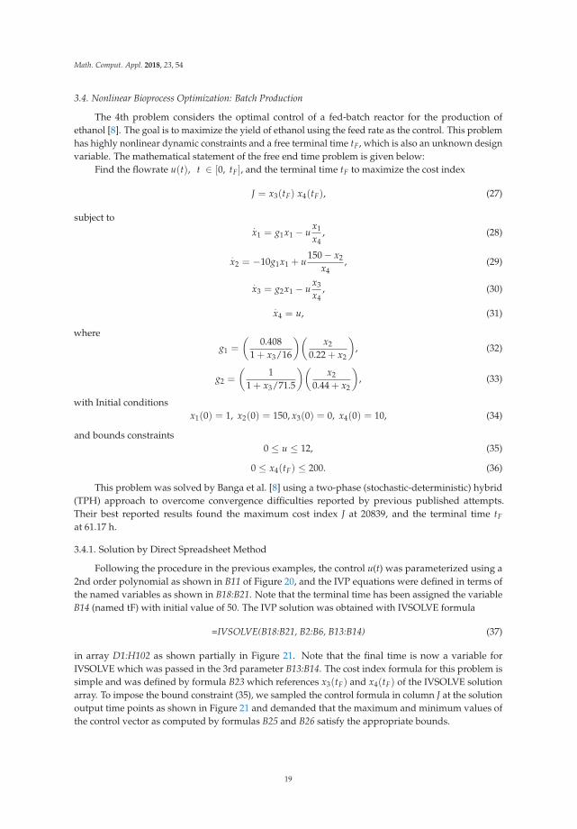
3.4. Nonlinear Bioprocess Optimization: Batch Production
The 4th problem considers the optimal control of a fed-batch reactor for the production ofethanol [8]. The goal is to maximize the yield of ethanol using the feed rate as the control. This problemhas highly nonlinear dynamic constraints and a free terminal time tF, which is also an unknown designvariable. The mathematical statement of the free end time problem is given below:
Find the flowrate u(t), t ∈ [0, tF], and the terminal time tF to maximize the cost index
J = x3(tF) x4(tF), (27)
subject to.x1 = g1x1 − u
x1
x4, (28)
.x2 = −10g1x1 + u
150 − x2
x4, (29)
.x3 = g2x1 − u
x3
x4, (30)
.x4 = u, (31)
where
g1 =
(0.408
1 + x3/16
)(x2
0.22 + x2
), (32)
g2 =
(1
1 + x3/71.5
)(x2
0.44 + x2
), (33)
with Initial conditionsx1(0) = 1, x2(0) = 150, x3(0) = 0, x4(0) = 10, (34)
and bounds constraints0 ≤ u ≤ 12, (35)
0 ≤ x4(tF) ≤ 200. (36)
This problem was solved by Banga et al. [8] using a two-phase (stochastic-deterministic) hybrid(TPH) approach to overcome convergence difficulties reported by previous published attempts.Their best reported results found the maximum cost index J at 20839, and the terminal time tFat 61.17 h.
3.4.1. Solution by Direct Spreadsheet Method
Following the procedure in the previous examples, the control u(t) was parameterized using a2nd order polynomial as shown in B11 of Figure 20, and the IVP equations were defined in terms ofthe named variables as shown in B18:B21. Note that the terminal time has been assigned the variableB14 (named tF) with initial value of 50. The IVP solution was obtained with IVSOLVE formula
=IVSOLVE(B18:B21, B2:B6, B13:B14) (37)
in array D1:H102 as shown partially in Figure 21. Note that the final time is now a variable forIVSOLVE which was passed in the 3rd parameter B13:B14. The cost index formula for this problem issimple and was defined by formula B23 which references x3(tF) and x4(tF) of the IVSOLVE solutionarray. To impose the bound constraint (35), we sampled the control formula in column J at the solutionoutput time points as shown in Figure 21 and demanded that the maximum and minimum values ofthe control vector as computed by formulas B25 and B26 satisfy the appropriate bounds.
19

Math. Comput. Appl. 2018, 23, 54
A B 1 ODE system variables with initial conditions 2 t 0 3 x_1 1 4 x_2 150 5 x_3 0 6 x_4 10 7 Parametrized controllers with starting guess 8 c_0 3 9 c_1 0
10 c_2 0 11 u =c_0+c_1*t+c_2*t^2 12 ODE time domain with final time guess 13 ts 0 14 tF 50 15 ODE system equations 16 g1_ =(0.408/(1+x_3/16))*(x_2/(0.22+x_2)) 17 g2_ =(1/(1+x_3/71.5))*(x_2/(0.44+x_2)) 18 x1dot =g1_*x_1-u*x_1/x_4 19 x2dot =-10*g1_*x_1+u*(150-x_2)/x_4 20 x3dot =g2_*x_1-u*x_3/x_4 21 x4dot =u 22 Cost Index 23 J =G102*H102 24 Constraints helpers 25 max(u) =MAXA(J2:J102) 26 min(u) =MINA(J2:J102)
Figure 20. Spreadsheet parametrized model for problem 3.4. The colored ranges are inputs forIVSOLVE formula (37).
D E F G H I J 1 t x_1 x_2 x_3 x_4 u 2 0 1 150 0 10 3 3 0.5 1.062808 148.0676 0.478626388 11.5 3 4 1 1.142691 146.2653 0.936035562 13 3
100 49 15.05587 0.078212 73.9061806 157 3 101 49.5 15.05539 0.077045 73.75951155 158.5 3 102 50 15.05491 0.07591 73.61434682 160 3
=IVSOLVE(B18:B21,B2:B6,B13:B14)
=c_0+c_1*D2+c_2*D2^2
Figure 21. Partial display of IVP (28)–(34) solution obtained by IVSOLVE formula (37), and generatedvalues for the parametrized control of problem 3.4.
20

Math. Comput. Appl. 2018, 23, 54
3.4.2. Results and Analysis
Excel solver was run starting from the initial guess for the unknown control coefficients andterminal time shown in Figure 20. The cost index J (B23) was selected to be maximized by varying theterminal time tF (B14), and the coefficients c_0, c_1 and c_2, (B8:B10) subject to the constraints:
B25 <= 12, corresponding to (35)
B26 >= −12, corresponding to (35)
H102 <= 200, corresponding to (36).
Excel NLP solver converged in approximately 29 s to the result shown in Figure 22, and plottedin Figure 23. A partial listing of the converged control values and IVP solution reflecting the newterminal time is shown in Figure 24.
Figure 22. Answer report generated by Excel solver for problem 3.4.
21

Math. Comput. Appl. 2018, 23, 54
Figure 23. Optimal trajectories computed by the spreadsheet method for problem 3.4.
D E F G H I J 1 t x_1 x_2 x_3 x_4 u 2 0 1 150 0 10 -0.44065 3 0.616388 1.313316 147.1366 0.712647865 9.737328 -0.41144 4 1.232776 1.702539 143.5086 1.64960033 9.49305 -0.38097
100 60.40604 14.84059 2.12186 102.2278477 189.4647 8.393491 101 61.02243 14.88833 1.630308 102.4917196 194.6852 8.545821 102 61.63882 14.925 1.25 102.6127698 200 8.699408
Figure 24. Partial listing of the converged IVP solution and control values of problem 3.4.
The achieved maxima for the cost index was at 20522.5 and the terminal time tF was found atapproximately 61.64. These values are in very good agreement with the best results reported byBanga et al. [8] at 20839, and 61.17 h. Figure 25 shows direct comparison of the states and controltrajectories with digitized plot values from Banga et al. The agreement is quite good for the mostpart despite fundamentally different control parametrization and algorithms employed by the twomethods. In particular, the control parametrization in [8] is approximated by connected line segments,whereas our control is a continuous parabola.
22

Math. Comput. Appl. 2018, 23, 54
Figure 25. Direct comparison of spreadsheet solution with reported solution obtained by Banga et al.for problem 3.4.
4. Conclusions
We devised a practical and systematic spreadsheet solution strategy for solving general optimalcontrol problems. The strategy is based on an adaptation of the partial-parametrization directsolution method which preserves the structure of the original mathematical optimization statement,but transforms it into a simplified NLP problem suitable for Excel NLP solver. The solution strategyis formulated by the aid of several elementary calculus functions from an available Excel calculusAdd-in [11] for solving differential equations, computing integrals and derivatives. The calculusfunctions are employed as building blocks in a hierarchical functional paradigm implemented bystandard Excel formulas in conjunction with Excel built-in NLP solver to carry out a dynamicoptimization program.
Results were obtained for four representative problems selected to illustrate modeling of severalconditions including dependence on higher order derivatives of state and controls as well as implicitIVP problems and integral constraints. The results were compared with published solutions obtainedby other methods, and in some cases, were shown to be better by the measure of the cost index.The performance of the method is also notable with computing times on the order of seconds toa minute on a standard laptop. As has been illustrated by the solution procedure, applying thetechnique involves no more than defining a few formulas that parallel the original mathematicalequations. No special programming skill is needed beyond basic familiarity with the commonspreadsheet operation. The minimal problem setup effort, in combination with the ubiquity of
23

Math. Comput. Appl. 2018, 23, 54
Excel spreadsheet, present reasons to explore the method as an alternative, simpler educational toolfor rather complex problems.
The success of the devised strategy for optimal control of ordinary differential equations supportsfuture research for extending the strategy to optimal control of partial differential equations. In [22],the author demonstrated an analogous formulation combing the NLP solver with a PDE solver fromthe same Add-in [11] for parameter estimation of partial differential algebraic equations, and it may befeasible that certain formulations of optimal control of partial differential equations are solvable in thespreadsheet by a similar strategy. On the other hand, it is worth investigating devising an alternativestrategy based on the indirect solution method [4,5] for optimal control problems. The indirect methodrequires solving a boundary value problem which could be solved by the aid of a boundary valueproblem solver function also available in the Excel calculus Add-in [11].
Supplementary Materials: An Excel workbook containing the solved problems in this paper is available onlineat http://www.mdpi.com/2297-8747/23/4/54/s1.
Funding: This research received no external funding.
Conflicts of Interest: The author of the manuscript is the founder of ExcelWorks LLC of Massachusetts, USAsupplying the Excel calculus Add-in [11], utilized in this research work.
Appendix A
The following subsections present brief descriptions of the calculus functions utilized in thiswork. The functions are enabled as an extension of Excel math functions by installing ExceLab calculusAdd-in [11]. For more detailed descriptions of the functions, the reader is referred to [11].
Appendix A.1 IVSOLVE: Initial Value Problem Solver
The worksheet function IVSOLVE solves an initial value differential algebraic equation system inthe interval t ∈
[ts, t f
]M dx
dt = F(x(t), t)x(t0) = x0
(A1)
x(t) = (x1(t), x2(t), . . . , xn(t)), and M is an optional mass matrix which may be singular. IVSOLVEuses by default RADUA5 an implicit 5th-order Runge-Kutta scheme with adaptive time step [15],and at minimum, requires three input parameters to describe the ODE system:
1. Reference to the right-hand side formulas corresponding to the vector-valued functionF(x(t), t) = ( f1(x(t), t), f2(x(t), t), . . . , fn(x(t), t)).
2. Reference to the system variables in the specific order (t, x1, x2, . . . , xn).3. The integration time interval end points.
Additional optional parameters include specifying a mass matrix as well as algorithmic controls.IVSOLVE is run as an array formula in an allocated array of cells. It evaluates to an ordered tabularresult where the time values are listed in the first column, and the corresponding state variables’ valuesare listed in adjacent columns. By default, IVSOLVE reports the output at uniform intervals accordingto the allocated number of rows for the output array. Custom output formats can be achieved via theoptional parameters including specifying custom divisions or exact points. We demonstrate IVSOLVEfor the following DAE problem (reproduced from [14]):
dy1dt = −0.04y1 + 104y2y3, t ∈ [0, 1000]
dy2dt = 0.04y1 − 104y2y3 − 3 ∗ 107y2
20 = y1 + y2 + y3 − 1
y1(0) = 1, y2(0) = 0, y3(0) = 0
(A2)
24

Math. Comput. Appl. 2018, 23, 54
Referring to Figure A1, the system RHS formulas are defined in cells A1:A3 using cell T1 for thetime variable and Y1, Y2, Y3 for the state variables which are assigned the initial conditions as shownin the figure.
Figure A1. Spreadsheet model for equation system (A2).
To solve the system, we execute the array formula
=IVSOLVE (A1:A3, (T1,Y1:Y3), {0,1000}, 1)
in an allocated array, (e.g., C1:F22) by pressing the 3 keys Control+Shift+Enter simultaneously.IVSOLVE computes and displays the solution shown Figure A2. Here we have used the 4th optionalparameter to specify that the last equation, (A3) is an algebraic equation.
Figure A2. Partial listing of the result computed by IVSOLVE (left) for system (A2), and a plot of thetrajectories (right).
Appendix A.2 QUADF: Formula Integrator Function
The spreadsheet function QUADF computes definite and improper one-dimensional integrals∫ ba f (x)dx. QUADF utilizes QUADPACK numerical integration algorithms [17] suitable for smooth,
irregular, and integrands with known singularities. By default, it uses QAG, an adaptive algorithmusing Gauss-Kronrod 21-point integration rule. We demonstrate QUADF by computing the followingintegral (reproduced from [14]):
1∫0
ln x√x
dx = −4 (A3)
Referring to Figure A3, the integrand formula is defined in cell A1 using X1 as dummy variable for theintegration. The QUADF integration formula
=QUADF (A1, X1, 0, 1)
is defined in A2 passing in the integrand formula, the variable of integration, and values for the limits.Evaluating A2 yields the result.
25

Math. Comput. Appl. 2018, 23, 54
Figure A3. Demonstration of QUADF for computing integral (A3) in Excel.
Using recursion, multiple integrals of any order can be computed by direct nesting of QUADF,as demonstrated by the following volume integral example:
2∫0
3− 32 x∫
0
6−3x−2y∫0
1 − x dz dy dx = 3 (A4)
To compute (A4), we construct a simple program consisting of three nested calls of QUADF as shownin Figure A4. Using X1, Y1 and Z1 as dummy variables, the integrand formula is defined in A1, and theinner, middle, and outer integrals formulas are defined in A2, A3 and A4 respectively, with each innerQUADF formula serving as the integrand for the next outer QUADF formula. Evaluating the outerintegral in A4 computes the triple integral value.
Figure A4. Demonstration of QUADF for computing multiple integral (A4) in Excel.
Appendix A.3 QUADXY: Discrete Data Integrator
The spreadsheet function QUADXY computes the integral of a curve passing through the set ofdata pairs (xi, yi(xi)), i = 0.. n. The integration interval is defined by the endpoints [x0, xn]. QUADXYcomputes the integral by the aid of cubic (default) or linear splines fit to the data [16]. Start and endpoint slope information may be specified in the 3rd optional parameter to enhance accuracy near theend points. The slope data is defined by a reference to a key/value array as illustrated in Figure A5.
Figure A5. Optional input format to QUADXY for endpoints boundary conditions.
For example, the formula
=QUADXY(X1:X20, Y1:Y20, C1:D2)
computes an integral value of 20 data pairs in columns X1 and Y1 with supplied optional end pointsslope values shown in Figure A5.
Appendix A.4 DERIVXY: Discrete Data Differentiator
The spreadsheet function DERIVXY employs cubic splines to compute the dth derivative of acurve passing through a set of data pairs (xi, yi(xi)), i = 0..n at a specified point x = p. Similar to
26

Math. Comput. Appl. 2018, 23, 54
QUADXY, optional start and or endpoint slope information may be specified to enhance accuracy nearthe end points. For example, the formula
=DERIVXY(X1:X20, Y1:Y20, 5, 2)
computes the second derivative for a curve passing through 20 points in columns X1 and Y1 at thepoint x = 5.
When using DERIVXY with Excel AutoFill feature to differentiate a given data set at multiplepoints, it is necessary to lock the parameters except for the variable point (parameter 3) so they are notincremented during the AutoFill. For example, the following formula is safe to use with AutoFill togenerate derivatives at points stored in Z1, Z2, Z3, etc.
=DERIVXY($X$1:$X$20, $Y$1:$Y$20, Z1)
References
1. Geering, H.P. Optimal Control with Engineering Applications; Springer: Berlin, Germany, 2007.2. Sethi, S.P. Optimal Control Theory: Applications to Management Science and Economics, 3rd ed.; Springer: Berlin,
Germany, 2019.3. Anita, S.; Arnăutu, V.; Capasso, V. An Introduction to Optimal Control Problems in Life Sciences and Economics:
From Mathematical Models to Numerical Simulation with MATLAB; Birkhäuser: Basel, Switzerland, 2011.4. Betts, J.T. Practical Methods for Optimal Control and Estimation Using Nonlinear Programming, 2nd ed.; Advances
in Design and Control; Society for Industrial and Applied Mathematics: Philadelphia, PA, USA, 2009.5. Böhme, T.J.; Frank, B. Indirect Methods for Optimal Control. In Hybrid Systems, Optimal Control and Hybrid
Vehicles. Advances in Industrial Control; Springer: Cham, Switzerland, 2017.6. Elnagar, G.; Kazemi, M.A. Pseudospectral Chebyshev Optimal Control of Constrained Nonlinear Dynamical
Systems. Comput. Optim. Appl. 1998, 11, 195–217. [CrossRef]7. Böhme, T.J.; Frank, B. Direct Methods for Optimal Control. In Hybrid Systems, Optimal Control and Hybrid
Vehicles. Advances in Industrial Control; Springer: Cham, Switzerland, 2017.8. Banga, J.R.; Balsa-Canto, E.; Moles, C.G.; Alonso, A.A. Dynamic optimization of bioprocesses: Efficient and
robust numerical strategies. J. Biotechnol. 2003, 117, 407–419. [CrossRef] [PubMed]9. Rodrigues, H.S.; Torres Monteiro, M.T.; Torres, D.F.M. Optimal Control and Numerical Software: An
Overview. arXiv, 2014; arXiv:1401.7279.10. Ghaddar, C.K. Novel Spreadsheet Direct Method for Optimal Control Problems. Math. Comput. Appl. 2018,
23, 6. [CrossRef]11. ExcelWorks LLC, MA, USA. ExceLab Calculus Add-in and Reference Manual. Available online: https:
//excel-works.com (accessed on 22 September 2018).12. Nævdal, E. Solving Continuous Time Optimal Control Problems with a Spreadsheet. J. Econ. Educ. 2003,
34, 2. [CrossRef]13. Weber, E.J. Optimal Control Theory for Undergraduates Using the Microsoft Excel Solver Tool. Comput. High.
Educ. Econ. Rev. 2007, 19, 4–15.14. Ghaddar, C. Unconventional Calculus Spreadsheet Functions. World Academy of Science, Engineering
and Technology, International Science Index 112. Int. J. Math. Comput. Phys. Electr. Comput. Eng. 2016,10, 194–200.
15. Hairer, E.; Wanner, G. Solving Ordinary Differential Equations II: Stiff and Differential-Algebraic Problems; SpringerSeries in Computational Mathematics; Springer: Berlin, Germany, 1996.
16. De Boor, C. A Practical Guide to Splines (Applied Mathematical Sciences); Springer: Berlin, Germany, 2001.17. Piessens, R.; de Doncker-Kapenga, E.; Ueberhuber, C.W.; Kahaner, D.K. Quadpack: A Subroutine Package for
Automatic Integration; Springer: Berlin, Germany, 1983.18. Lasdon, L.S.; Waren, A.D.; Jain, A.; Ratner, M. Design and Testing of a Generalized Reduced Gradient Code
for Nonlinear Programming. ACM Trans. Math. Softw. 1978, 4, 34–50. [CrossRef]19. Dolan, E.D.; More, J.J. Benchmarking Optimization Software with Cops; Technical Report; Argonne National
Laboratory: Argonne, IL, USA, 2001.
27

Math. Comput. Appl. 2018, 23, 54
20. Lim, A.E.B.; Liu, Y.Q.; Teo, K.L.; B, M.J. Linear-quadratic optimal control with integral quadratic constraints.Optim. Control Appl. Methods 1999, 20, 79–92. [CrossRef]
21. Bhattacharya, R. OPTRAGEN 2.0: A MATLAB Toolbox for Optimal Trajectory Generation; Texas A & MUniversity: College Station, TX, USA, 2013.
22. Ghaddar, C.K. Rapid Modeling and Parameter Estimation of Partial Differential Algebraic Equations by aFunctional Spreadsheet Paradigm. Math. Comput. Appl. 2018, 23, 39. [CrossRef]
© 2018 by the author. Licensee MDPI, Basel, Switzerland. This article is an open accessarticle distributed under the terms and conditions of the Creative Commons Attribution(CC BY) license (http://creativecommons.org/licenses/by/4.0/).
28

Mathematical
and Computational
Applications
Article
Novel Spreadsheet Direct Method for OptimalControl Problems
Chahid Kamel Ghaddar
ExcelWorks LLC, Sharon, MA 02067, USA; [email protected]; Tel.: +1-781-626-0375
Received: 26 December 2017; Accepted: 23 January 2018; Published: 25 January 2018
Abstract: We devise a simple yet highly effective technique for solving general optimal controlproblems in Excel spreadsheets. The technique exploits Excel’s native nonlinear programming(NLP) Solver Command, in conjunction with two calculus worksheet functions, namely, an initialvalue problem solver and a discrete data integrator, in a direct solution paradigm adapted to thespreadsheet. The technique is tested on several highly nonlinear constrained multivariable controlproblems with remarkable results in terms of reliability, consistency with pseudo-spectral reportedanswers, and computing times in the order of seconds. The technique requires no more than defininga few analogous formulas to the problem mathematical equations using basic spreadsheet operations,and no programming skills are needed. It introduces an alternative, simpler tool for solving optimalcontrol problems in social and natural science disciplines.
Keywords: optimal control; dynamical optimization; parameter estimation; differential equations;spreadsheet; Excel Solver
1. Introduction
Optimal control problems are commonly encountered in engineering and life sciences, as well associal studies such as economics and finance [1–3]. An optimal control problem is typically concernedwith finding optimal control functions (or policies) that achieve optimal trajectories for a set ofcontrolled differential state variables. The optimal trajectories are decided by a constrained dynamicaloptimization problem, such that a cost functional is minimized or maximized subject to certainconstraints on state variables and the control functions. Mathematically, an optimal control problemmay be stated as follows:
Find the control functions u(t) = (u1(t), u2(t), . . . , um(t)) and the corresponding state variablesx(t) = (x1(t), x2(t), . . . , xn(t)), t ∈ [0, T] which minimize (or maximize) the functional
J = H(x(T), T) +T∫
0
G(x(t), u(t), t) dt, (1)
subject to
Mdxdt
= F(x(t), u(t), t), (2)
with initial conditionsx(0) = x0, (3)
and optional final conditions and bounds
Q(x(T), T) = 0, (4)
S(x(t), u(t)) ≤ 0. (5)
Math. Comput. Appl. 2018, 23, 6; doi:10.3390/mca23010006 www.mdpi.com/journal/mca29

Math. Comput. Appl. 2018, 23, 6
In the formulation (1)–(5), the generally nonlinear H and G are scalar functions, whereas F, Q,and S are vector-valued functions. Typically, either H or Q are specified but not both in the sameproblem. Common forms of Q and S are x(T) = xT and umin ≤ u(t) ≤ umax, respectively. We havechosen not to include
.x(t) and
..x(t) in the formulation because a higher-order explicit differential
equation system can be restated as a first-order system via variable substitution. The matrix M in (2)offers an optional coupling of the states’ temporal derivatives by a mass matrix which may be singular.If M is singular, the equation system (2) is differential algebraic, or DAE. For uncoupled derivatives,M is the identity matrix which can be omitted. Furthermore, T, which denotes the final time, may befixed or free.
Numerical solution strategies of (1)–(5) fall into one of two approaches: an indirect method,where Pontryagin’s minimum principle is employed to transform the problem into an augmentedHamiltonian system requiring the solution of a boundary value problem [4]; and a direct method,where the original system’s variables are approximated by parameterized appropriate functionswhich, in turn, reduce the problem into a finite-dimensional nonlinear programming problem [5].Direct methods can be further classified as full or partial parametrization methods. In the latter,only the controls are parametrized, wherein the inner initial value problem (IVP) (2)–(3) is treated asa separate dependent problem that must be solved repeatedly by the outer nonlinear programming(NLP) algorithm [6].
Except for the most trivial cases, optimal control problems can be difficult to solve, particularlyfor those who are not inclined towards programming and numerical methods. Despite advances insoftware programs, it remains a nontrivial task to utilize a standard package such as MATLAB to solveoptimal control problems. The student must have sufficient programming skill, as well as a goodunderstanding of the general structure of the solution algorithm and the various solvers required toimplement it [7].
In this article, we present a systematic technique for solving optimal control problems in aspreadsheet, modeled on partial parametrization direct methods. The technique is made possible,on the one hand, by algorithmic advances [8,9] which enabled the introduction of mathematically purecalculus worksheet functions to the spreadsheet [10,11]. A pure calculus function is evaluated as astandard built-in math function; however, it accepts, via input parameters, formulas representing aproblem model and outputs a formatted solution result. Specifically, we make use of two calculusfunctions described in Appendix A: an IVP solver, based on an implicit RADUA5 algorithm withadaptive step control [12], which we employ for solving the inner IVP (2)–(3); and a discrete dataintegrator, based on cubic spline approximations [13], which we employ to approximate the cost index(1). On the other hand, Excel spreadsheets include a powerful NLP Solver Command based on theGeneralized Reduced Gradient Method (GRG) [14] which is compatible with the calculus functions.We devise a direct control–parametrization method based on employing the calculus functions withthe NLP Solver in a dynamical optimization paradigm for the solution of (1)–(5).
Attempts to solve optimal control problems in spreadsheets are not new; however, to the best ofour knowledge, no prior work has presented a practical direct spreadsheet method aimed at solvingthe general nonlinear multidimensional optimal control problem (1)–(5). The chief reason is that priorapproaches utilized the spreadsheet explicitly as the computational grid for the discretization andsolution of the underlining IVP. This limits the practical scope to rather simple problems that can beeasily discretized with an explicit differencing scheme suitable for the spreadsheet. For example,Weber [15] demonstrated a direct approach to solving control problems in resource economicsinvolving simple one-dimensional IVPs, and direct summation of discrete values for the cost index.Nævdal [16] demonstrated a basic implementation of the indirect method, with the aid of Visual Basicfor Applications (VBA) programming, to solve one-dimensional optimal control problems. The methodutilized Excel’s Solver in conjunction with an explicit difference scheme and a shooting algorithm tosolve the resulting boundary value problem. While Nævdal’s work provides educational insights intothe mechanics of the indirect solution method, its detail-intensive implementation makes it impractical
30

Math. Comput. Appl. 2018, 23, 6
to use or extend to higher dimensions or nonlinear stiff systems requiring adaptive implicit schemes.Our devised direct spreadsheet method, on the other hand, differs fundamentally from prior work,in that the algorithmic implementation for solving the IVP, and integrating the cost index, has beendecoupled from the spreadsheet grid and encapsulated in pure spreadsheet solver functions suitablefor seamless integration with the NLP Solver. The design of the solver functions, described in Section 2,permits utilization of fully implicit and adaptive algorithms which make the method applicable toa general class of nonlinear multivariable optimal control problems. Furthermore, by encapsulatingthe tedious implementation details in standard pure math functions with a clear divide betweeninput and output, the method is applicable with little more than basic spreadsheet knowledge, andwithout any programming skills. As demonstrated in Section 3, results obtained on several highlynonlinear problems are remarkable, in terms of both the reliability and the computing time in the orderof seconds. The devised method extends the utility of the spreadsheet beyond what has been practicalor even feasible before.
The remainder of this paper is organized as follows: In the next section, we describe the basic stepsrequired to model and solve an optimal control problem using the adapted direct method technique.In Section 3, we demonstrate the technique for solving four different control problems reproducedfrom Elnagar and Kazemi [17] who used a pseudo-spectral direct method. The problems include:
1. A bang–bang control problem.2. A highly nonlinear and coupled system.3. A minimum swing container transfer problem involving multiple controls and constraints.4. A minimum time orbit transfer control problem with free end time.
Section 4 provides some practical tips for applying the technique, followed by conclusions inSection 5. Appendix A includes a description for the IVP solver, IVSOLVE, and the discrete dataintegrator functions, QUADXY, both of which are essential for the technique. We also remark that ourmain focus in this first article is to introduce and illustrate the spreadsheet direct solution method ratherthan formulate or study any specific optimal control problem. As such, we start from a mathematicalstatement of a given problem and present a feasible solution obtained by the method with relevantcomparisons to the reported result in [17].
2. Spreadsheet-Adapted Direct Solution Method
The main enabling elements of the devised method are, in addition to the NLP Solver, the IVPsolver function, IVSOLVE, and the discrete data integrator, QUADXY. The IVSOLVE spreadsheetfunction, described in Appendix A.1, is designed according to the flowchart of Figure 1, wherein asuitable highly accurate algorithm, such as RADUA5 [12], is fully shielded with a strict divide betweenthe IVP model input and the output solution results. The model input is represented by formulas thatare direct analogues to the IVP mathematical equations, and the output solution results are displayed ina formatted tabular array of elective resolution which is easily adjusted to yield an accurate integrationof a dependent cost index. By design, IVSOLVE is a pure function which does not modify its inputbut merely computes and displays the solution in its allocated spreadsheet array. QUADXY, on theother hand, follows a standard spreadsheet User Defined Function (UDF) implementation to integratea vector of ordered points, (t, y(t))i, i = 1, n. QUADXY performs the integration with the aid ofcubic splines fit to the data. Under the assumption that the discrete data describe a smooth curve,the computed integral is generally quite accurate and can be further improved by supplying optionalslopes at the end points of the curve when they are known or can be estimated. Likewise, QUADXY isalso a pure function which does not modify its inputs.
Below, we describe the general steps for employing IVSOLVE and QUADXY with the NLP Solverfor solving the optimal control problem (1)–(5). Some of these steps may or may not be required for agiven problem. To simplify the discussion, we shall assume a single control function, u(t). Extension to
31

Math. Comput. Appl. 2018, 23, 6
multiple controls is straightforward and is demonstrated by the examples. In practice, there are threesystematic tasks:
Task 1
The first step is to obtain, with the IVP solver function, IVSOLVE, an initial solution for theunderlining IVP (2)–(3) using an appropriately parametrized formula for the control function and initialguesses for the unknown parameters. A continuous control function can be parametrized, for example,by a third-order polynomial with unknown coefficients, such as ‘=c_0+c_1*t+c_2*tˆ2+c_3*tˆ3’. On theother hand, a discontinuous control function can be modeled using the standard IF statement in Excel.For example, a two-stage, constant controller can be defined as follows: ‘=IF(t<=ts,value1,value2)’.Here ts, value1, and value2 are unknown parameters that would be assigned initial guesses.
Task 2
In the second task we define an analogous objective formula for the cost functional (1).Our strategy is to integrate, using QUADXY, a sampled vector of the integrand expression in (1)using the solution values obtained in Task 1. To accomplish this, in a new column, we generate valuesfor the parametrized control formula evaluated at the solution’s output times and, in a second column,we generate values for the integrand expression, using the solution’s state variables and generatedcontrol values as needed. Both the control and integrand columns are easily generated using theAutoFill feature of Excel. To define an analogous objective formula for the cost index (1), we employthe discrete data integrator function, QUADXY, to integrate the generated integrand data columnversus the solution’s output times column. The ordered steps needed to define the objective formulaare summarized in Figure 2.
Task 3
The last task is to configure and run Excel’s NLP Solver. The NLP Solver can be configuredto minimize or maximize an objective formula by changing design variables, subject to definedconstraints. The design variables are the unknown parameters which are assigned initial guessesin Task 1. The constraints (4) and (5) are added directly in the Solver’s dialog. Simple equality endconditions on state variables are added by referencing the corresponding cells in the solution output asillustrated in Figure 2. Bound constraints on state variables or controls are easily imposed with the aidof Excel’s MAXA() and MINA() math functions which compute the maximum and minimum values ofa vector. Concrete examples are presented in the next section.
Figure 1. Flowchart for the design of a mathematically pure spreadsheet solver function which acceptsformulas as input arguments. Enabling technology is described in [8,9].
32
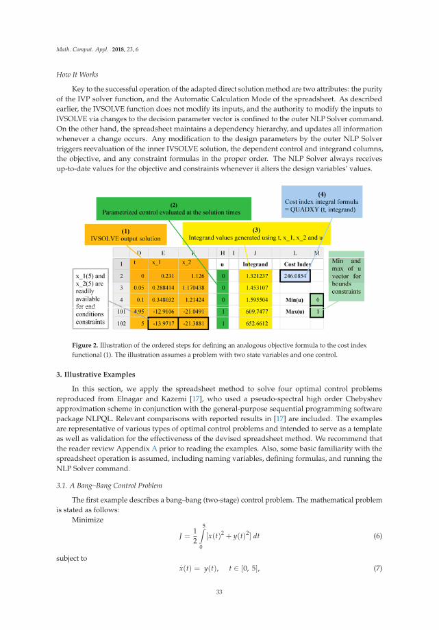
Math. Comput. Appl. 2018, 23, 6
How It Works
Key to the successful operation of the adapted direct solution method are two attributes: the purityof the IVP solver function, and the Automatic Calculation Mode of the spreadsheet. As describedearlier, the IVSOLVE function does not modify its inputs, and the authority to modify the inputs toIVSOLVE via changes to the decision parameter vector is confined to the outer NLP Solver command.On the other hand, the spreadsheet maintains a dependency hierarchy, and updates all informationwhenever a change occurs. Any modification to the design parameters by the outer NLP Solvertriggers reevaluation of the inner IVSOLVE solution, the dependent control and integrand columns,the objective, and any constraint formulas in the proper order. The NLP Solver always receivesup-to-date values for the objective and constraints whenever it alters the design variables’ values.
Figure 2. Illustration of the ordered steps for defining an analogous objective formula to the cost indexfunctional (1). The illustration assumes a problem with two state variables and one control.
3. Illustrative Examples
In this section, we apply the spreadsheet method to solve four optimal control problemsreproduced from Elnagar and Kazemi [17], who used a pseudo-spectral high order Chebyshevapproximation scheme in conjunction with the general-purpose sequential programming softwarepackage NLPQL. Relevant comparisons with reported results in [17] are included. The examplesare representative of various types of optimal control problems and intended to serve as a templateas well as validation for the effectiveness of the devised spreadsheet method. We recommend thatthe reader review Appendix A prior to reading the examples. Also, some basic familiarity with thespreadsheet operation is assumed, including naming variables, defining formulas, and running theNLP Solver command.
3.1. A Bang–Bang Control Problem
The first example describes a bang–bang (two-stage) control problem. The mathematical problemis stated as follows:
Minimize
J =12
5∫0
[x(t)2 + y(t)2] dt (6)
subject to.x(t) = y(t), t ∈ [0, 5], (7)
33

Math. Comput. Appl. 2018, 23, 6
.y(t) = y(t)− x(t) + u(t), (8)
x(0) = 0.231, y(0) = 1.126, (9)
− 0.8 ≤ u(t) ≤ 0.8. (10)
3.1.1. Spreadsheet Model
Working with named variables with adjacent labels shown in Column A of Figure 3,we parametrized the two-stage control function, u(t), using a standard IF() statement, as shownin B9. The unknown parameters switchT, stage1, and stage2 were assigned the initial guess values0.1, 0, and 1. The right-hand sides of the IVP differential Equations (7) and (8) were represented bythe equivalent formulas B11 and B12, and the initial conditions (9) were assigned to the variables xand y in B3 and B4. The colored ranges in Figure 3 represent the model input required to obtain theinitial solution for the IVP (7)–(9) using the IVSOLVE function. The initial solution was obtained byevaluating the formula
=IVSOLVE(B11:B12,B2:B4,{0,5}) (11)
in an allocated array D2:F103. The result is shown partially in Figure 4, and the initial trajectories ofx(t), y(t), and u(t) are plotted in Figure 7a.
A B 1 ODE variables 2 t 03 x 0.2314 y 1.1265 Parametrized control formula 6 switchT 0.17 stage1 08 stage2 19 u =IF(t<=switchT,stage1,stage2)
10 ODE rhs formulas 11 xdot =y 12 ydot =u x+y
Figure 3. Spreadsheet model for IVP (7)–(9) with parametrized control function. The colored rangesare input parameters for the IVSOLVE Formula (11).
D E F H J L M 1 IVP Solution 2 t x y u Integrand Cost functional3 0 0.231 1.126 0 1.321237 Objective 246.0854 4 0.05 0.288414 1.170438 0 1.453107 5 0.1 0.348032 1.21424 0 1.595504 Constraint formulas 6 0.15 0.411089 1.308339 1 1.880744 Max(u) 1 7 0.2 0.478891 1.403911 1 2.200301 Min(u) 0
102 4.95 12.9106 21.0491 1 609.7477 103 5 13.9717 21.3881 1 652.6612
Figure 4. Partial listing of computed results by Formula (11). Also shown are generated control andintegrand columns, and initial objective formula value. The associated formulas are listed in Table 1.
34

Math. Comput. Appl. 2018, 23, 6
In order to define the objective formula for the cost functional (6) as described in Task 2 ofSection 2, we first generated, based on the obtained initial solution array, two new columns labeledu and Integrand (see Figure 4) for the control function and the integrand expression. The controlcolumn, u, was generated with the AutoFill feature of Excel, using the formula H3 shown in Table 1.The integrand column was generated in a similar way using the formula J3 in Table 1. Here, we simplyevaluated the expression x(t)2 + y(t)2 using the corresponding output solution values for t, x, and yfrom the IVSOLVE solution.
Table 1. Formula definitions used for solving optimal control problem (6)–(10).
Purpose Cell Formula
Initial value problem solution D2:F103 =IVSOLVE(B11:B12,B2:B4,{0,5})AutoFill formula for control values H3 =IF(D3<=switchT,stage1,stage2)
AutoFill formula for integrand values J3 =E3ˆ2+F3ˆ2Objective formula M3 =0.5*QUADXY(D3:D103,J3:J103)
Maximum value of control column M6 =MAXA(H3:H103)Minimum value of control column M7 =MINA(H3:H103)
Next, we employed the discrete data integrator function QUADXY to integrate the generatedintegrand column versus the solution output times column, as shown by formula M3 of Table 1.The initial value of the objective formula was 246.0854, as shown in Figure 4. To impose the boundconstraint (10) on u(t), we defined two aid formulas in M6 and M7 (see Table 1) which computed themaximum and minimum of the generated control column values. We made use of these aid formulasduring the configuration of the NLP Solver.
3.1.2. Results and Discussion
We invoked Excel’s Solver from the Data Tab which brings up a dialog as shown in Figure 5.We configured the Solver to minimize the objective formula M3 by varying the control parametersB6:B8 (corresponding to switchT, stage1 and stage2) subject to the constraints
M6 ≤ 0.8 corresponds to max(u) ≤ 0.8, ()
M7 ≥ −0.8 corresponds to min(u) ≥ −0.8, ()
which are needed impose (10). We unchecked the box which reads ‘Make Unconstrained VariablesNon-Negative’ to allow the variables to take on negative values as well. In the options for the GRGNonlinear solver, we switched the derivative scheme from the default Forward to Central, and then ranthe Solver, which reports a feasible solution in less than 3 s. By accepting the Solver’s solution, all thevalues and plots in the spreadsheet were automatically updated to reflect the optimal result. The NLPSolver also generates an optional Answer Report, as shown in Figure 6. The optimal trajectoriesare plotted in Figure 7b. As shown in the Answer Report, the optimal switching time was found atapproximately 1.26 which is within 1% of the 1.25 value reported by Elnagar and Kazemi [17] using apseudo-spectral Chebyshev approximation of order 15. (In [17], the time domain was transformedto [−1, 1], and the switching time was found at negative 0.5 which maps to 1.25 in the original [0, 5]time domain.)
35

Math. Comput. Appl. 2018, 23, 6
Figure 5. Excel’s Solver dialog configured for optimal control problem (6)–(10).
Figure 6. Answer Report generated by Excel’s Solver for optimal control problem (6)–(10).
36

Math. Comput. Appl. 2018, 23, 6
(a) (b)
Figure 7. (a) Initial trajectories for optimal control problem (6)–(10) based on the default values shownin Figure 3; (b) Optimal trajectories found by Excel’s nonlinear programming (NLP) Solver.
3.2. Unconstrained Nonlinear Optimal Control Problem
The second example represents an unconstrained optimal control problem in the fixed intervalt ∈ [−1, 1], but with highly nonlinear equations. The mathematical problem is stated as follows:
Minimize
J =0.78
2
1∫−1
[x1(t)
2 + x2(t)2 + 0.1u(t)2
]dt (12)
subject to
.x1(t) =
0.782
(−2[x1(t) + 0.25] + [x2(t) + 0.5]exp
[25x1(t)
x1(t) + 2
]− [x1(t) + 0.25]u(t)
), (13)
.x2(t) =
0.782
(0.5 − x2(t)− [x2(t) + 0.25]exp
[25x1(t)
x1(t) + 2
]− [x1(t) + 0.25]
), (14)
x(−1) = 0.05, x2(−1) = 0.0. (15)
3.2.1. Spreadsheet Model
The spreadsheet model for the IVP (13)–(15) with a parametrized control function using athird-order polynomial is shown in Figure 8. The initial solution to the IVP was obtained by evaluatingthe formula
=IVSOLVE(B12:B13,B2:B4,{−1,1}) (16)
in an allocated array E2:G103, which is shown partially in Figure 9 and plotted in Figure 10a. Clearly,our initial guess for the control coefficients B6:B9 was not good, since the solution exhibits instabilitiesat larger time values. The control and integrand vectors, needed to construct the objective formula forthe cost index (12), were generated based on the obtained initial solution using formulas I3 and K3,listed in Table 2. The objective formula was defined using the data integrator QUADXY as shown inN3 of Table 2, with an initial value of 1.92 × 10¹⁸, as shown in Figure 9.
Table 2. Formula definitions used for solving optimal control problem (12)–(15).
Purpose Cell Formula
Initial value problem solution E2:G103 =IVSOLVE(B12:B13,B2:B4,{−1,1})AutoFill formula for control values I3 =c_0+c_1*E3+c_2*E3ˆ2+c_3*E3ˆ3
AutoFill formula for integrand values K3 =F3ˆ2+G3ˆ2+0.1*I3ˆ2Objective N3 =0.78*QUADXY(E3:E103,K3:K103)/2
37

Math. Comput. Appl. 2018, 23, 6
A B
1 ODE variables 2 t -1
3 x_1 0.05
4 x_2 0 5 Parametrized control formula6 c_0 1
7 c_1 0 8 c_2 0
9 c_3 0
10 u =c_0+c_1*t+c_2*t^2+c_3*t^311 ODE rhs equations 12 x1dot =0.78*( 2*(x_1+0.25)+(x_2+0.5)*EXP(25*x_1/(x_1+2)) (x_1+0.25)*u)/2
13 x2dot =0.78*(0.5 x_2 (x_2+0.25)*EXP(25*x_1/(x_1+2)))/2
Figure 8. Spreadsheet model for the IVP (13)–(15) with parametrized control function. The coloredranges are input parameters for IVSOLVE Formula (16).
E F G H I J K L M N
1 IVP Solution 2 t x_1 x_2 u Integrand Cost functional 3 1.00 0.05 0 1 0.1025 Objective 1.92396E+18
4 0.98 0.050163 0.000305 1 0.1025165 0.96 0.050341 0.000596 1 0.102535
100 0.94 3.59E+09 0.25 1 1.29E+19101 0.96 3.64E+09 0.25 1 1.33E+19
102 0.98 3.7E+09 0.25 1 1.37E+19
103 1.00 3.75E+09 0.25 1 1.41E+19
Figure 9. Partial listing of computed results by Formula (16). Also shown are generated control andintegrand columns, and the initial objective formula value. The associated formulas are listed in Table 2.
(a) (b)
Figure 10. (a) Initial trajectories for optimal control problem (12)–(15) based on the default valuesshown in Figure 8; (b) Optimal trajectories found by Excel’s NLP Solver.
3.2.2. Results and Discussion
We ran Excel’s Solver to minimize the objective formula N3 by varying the control parameters inB6:B9 with no added constraints. Despite the bad initial values for the control parameters, the Solver
38

Math. Comput. Appl. 2018, 23, 6
reported a feasible solution in about 2 seconds with the Answer Report shown in Figure 11. The optimaltrajectories for the system variables are plotted in Figure 10b.
Figure 11. Answer Report generated by Excel’s Solver for optimal control problem (12)–(15) based onthe initial guess values in Figure 8.
The reported objective in [17] is 0.026621417, which is better than the achieved objective value of0.08919 found by Excel. To improve the result, we tried a different initial guess for the parameters (c_0,c_1, c_2, c_3) by changing their values in Figure 8 to (1, 0, 1, 0). A second run of the Solver reportedthe feasible solution shown in Figure 12. The new objective value was reduced by more than 50% to0.040245. The new solution is plotted in Figure 13 and shows noticeably different trajectories for x_1and x_2 than those obtained initially in Figure 10. This is expected, given the highly nonlinear andunconstrained problem.
Figure 12. Answer Report for optimal control problem (12)–(15) using a different initial guess andyielding improved minimum.
39

Math. Comput. Appl. 2018, 23, 6
Figure 13. Optimal trajectories for optimal control problem (12)–(15) found by Excel’s Solver startingfrom a different initial guess, leading to a lower objective value.
3.3. Minimal Swing Container Transfer Problem
The third example represents the problem of transferring containers, driven by a hoist motor anda trolley drive motor, from a ship to a cargo truck. The goal is to minimize the swing during and at theend of the transfer. The mathematical optimal control problem is described by (17)–(29). The problemis nonlinear with six state variables and two controllers subject to multiple final and bound constraints.
Minimize
J = 4.51∫
0
[x3(t)2 + x6(t)
2] dt (17)
subject to.x1(t) = 9x4(t), (18).x2(t) = 9x5(t), (19).x3(t) = 9x6(t), (20)
.x4(t) = 9[u1(t) + x3(t)], (21)
.x5(t) = 9u2(t), (22)
.x6(t) =
9(u1(t) + 27.0756x3(t) + 2x5(t)x6(t))x2(t)
, t ∈ [0, 1]. (23)
Initial conditions:
x1(0) = 0, x2(0) = 22, x3(0) = 0, x4(0) = 0, x5(0) = −1, x6(0) = 0. (24)
Final conditions:
x1(1) = 10, x2(1) = 14, x3(1) = 0, x4(1) = 2.5, x5(1) = 0, x6(1) = 0. (25)
Bounds:|u1(t)| ≤ 2.83374, (26)
− 0.80865 ≤ u2(t) ≤ 0.71265, (27)
40

Math. Comput. Appl. 2018, 23, 6
|x4(t)| ≤ 2.5, (28)
|x5(t)| ≤ 1.0. (29)
3.3.1. Spreadsheet Model
Following the same procedure as that in the previous examples, we prepared the spreadsheetmodel for the IVP (18)–(24) using third-order parametrized polynomial control functions u1(t) andu2(t), as shown in Figure 14. Initial values and guesses were assigned to the state variables andunknown parametrization coefficients as shown in the figure. Figure 15 shows a partial listing of theinitial solution obtained by evaluating the formula
=IVSOLVE(B17:B22,B2:B8,{0,1}) (30)
in array F2:L103, and the generated control columns, u_1, u_2, and the integrand expression columnusing the corresponding formulas listed in Table 3. The initial system trajectories are plotted inFigure 16.
A B C D
1 ODE variables
2 t 0
3 x_1 0
4 x_2 22
5 x_3 0
6 x_4 0
7 x_5 1
8 x_6 0
9 Parametrized controls formulas
10 c_0 1 d_0 1
11 c_1 1 d_1 1
12 c_2 5 d_2 -5
13 c_3 5 d_3 -5
14 u_1 =c_0+c_1*t+c_2*t^2+c_3*t^3
15 u_2 =d_0+d_1*t+d_2*t^2+d_3*t^3
16 ODE rhs equations
17 x1dot =9*x_4
18 x2dot =9*x_5
19 x3dot =9*x_6
20 x4dot =9*(u_1+x_3)
21 x5dot =9*u_2
22 x6dot =9*(u_1+27.0756*x_3+2*x_5*x_6)/x_2
Figure 14. Spreadsheet model for the IVP (18)–(24) with parametrized control functions. The coloredranges are input parameters for IVSOLVE Formula (30).
Next, we defined the objective formula, S3, corresponding to the cost index (17) as shownin Table 3, in which the data integrator QUADXY was used to integrate the generated integrandexpression values. The objective formula evaluated to an initial value of 24,229.22793. Table 3 also listsa number of aid formulas which compute the minimum and maximum values for the state variables
41

Math. Comput. Appl. 2018, 23, 6
x_4 and x_5 and the generated control columns. These aid formulas were used to define the boundconstraints for the NLP Solver.
F G H I J K L M N O P 1 IVP Solution 2 t x_1 x_2 x_3 x_4 x_5 x_6 u_1 u_2 Integrand3 0 0 22 0 0 1 0 1 1 04 0.01 0.004063 21.91406 0.000185 0.09044 0.90957 0.00411 1.009495 1.009495 1.69E-055 0.02 0.016305 21.8363 0.000742 0.181723 0.81832 0.008285 1.01796 1.01796 6.92E-056 0.03 0.036797 21.76679 0.001679 0.273786 0.72636 0.012569 1.025365 1.025365 0.000161
101 0.98 230.6731 15.34798 189.5472 205.5287 12.3527 147.8948 7.52796 7.52796 57801.01102 0.99 249.9267 14.20542 203.2503 222.511 13.0407 156.6717 7.762 7.762 65856.72103 1 270.7634 13 217.7568 240.7409 13.75 165.7417 -8 8 74888.35
Figure 15. Partial listing of computed result by Formula (30). Also shown are generated control andintegrand columns. The associated formulas are listed in Table 3.
Figure 16. Initial trajectories for optimal control problem (17)–(29) based on default values shown inFigure 14.
Table 3. Formulas definitions used for solving optimal control problem (17)–(29).
Purpose Cell Formula
Initial value problem solution F2:L103 =IVSOLVE(B17:B22,B2:B8,{0,1})AutoFill formula for u_1 control values N3 =c_0+c_1*F3+c_2*F3ˆ2+c_3*F3ˆ3AutoFill formula for u_2 control values O3 =d_0+d_1*F3+d_2*F3ˆ2+d_3*F3ˆ3AutoFill formula for integrand values P3 =I3ˆ2+L3ˆ2
Objective Formula S3 =4.5*QUADXY(F3:F103,P3:P103)u_1 column max value S6 =MAXA(N3:N103)u_1 column min value S7 =MINA(N3:N103)u_2 column max value S8 =MAXA(O3:O103)u_2 column min value S9 =MINA(O3:O103)x_4 column max value S10 =MAXA(J3:J103)x_4 column min value S11 =MINA(J3:J103)x_5 column max value S12 =MAXA(K3:K103)x_5 column min value S13 =MINA(K3:K103)
3.3.2. Results and Discussion
We configured Excel’s Solver to minimize the objective formula S3 by varying the controls’coefficients B10:B14 and D10:D14 subject to the added constraints listed in Table 4. Here, we made use
42

Math. Comput. Appl. 2018, 23, 6
of the aid formulas listed in Table 3 to define the inequality bound constraints (26)–(29). The end pointequality constraints on the state variables (25) were imposed directly onto the corresponding cells at t= 1 (last row) of the IVSOLVE solution array (see Figure 15). The Solver spun for a few seconds, thenreported that it did not find a feasible solution when, in fact, it already had, judging by the best-foundsolution results shown partially in Figure 17 and plotted in Figure 18. The solution indicates thatall constraints were satisfied within a reasonable tolerance of 1 × 10⁻⁵, except for x_6(1), which wassatisfied within a tolerance of 1 × 10⁻³. This is verified by the feasibility report generated by theSolver, and shown in Figure 19. The report indicates that the Solver had difficulty satisfying end pointconstraints for x_4 and x_6 at the Solver’s default tolerances, while all other constraints were satisfied.
Table 4. List of constraints added to the NLP Solver for optimal control problem (17)–(29) and theircorresponding equations. The bound constraints were defined using aid formulas listed in Table 3.
Added Constraints Purpose
G103 = 10 x1(1) = 10
H103 = 14 x2(1) = 14
I103 = 0 x3(1) = 0
J103 = 2.5 x4(1) = 2.5
K103 = 0 x5(1) = 0
L103 = 2.5 x6(1) = 0
S10 ≤ 2.5(4.12)S11 ≥ −2.5
S12 ≤ 1(4.13)S13 ≥ −1
S6 ≤ 2.83374(4.10)S7 ≥ −2.83374
S8 ≤ 0.71265(4.11)S9 ≥ −0.80865
Figure 17. Best-found solution obtained by Excel’s Solver for optimal control problem (17)–(29).
The reported objective in [17] is 0.005361, but the exact tolerances used for the NLPQL solverare unknown. We note that in this problem, Excel’s Solver best-found solution has a much lowerminimum for the objective at 0.000805, as shown in Figure 17.
43

Math. Comput. Appl. 2018, 23, 6
(a) (b)
Figure 18. (a) Optimal trajectories for all variables of optimal control problem (17)–(29); (b) Selectedoptimal trajectories.
Microsoft Excel 16.0 Feasibility Report
Worksheet: [Examples.xlsx]Example 3
Report Created: 9/26/2017 6:43:45 PM
Constraints Which Make the Problem Infeasible
Cell Name Cell Value Formula Status Slack
$H$103 x_2 14.00000001 $H$103=14 Binding 0 $J$103 x_4 2.499994248 $J$103=2.5 Violated 5.75165E-06
$L$103 x_6 0.00072322 $L$103=0 Violated 0.00072322
Figure 19. Feasibility Report generated by Excel’s Solver for optimal control problem (17)–(29).
3.4. Minimum Time Orbit Transfer Problem
The fourth example describes a minimum time orbit transfer problem. The goal is to minimizethe transfer time of a constant thrust rocket between the orbits of Earth and Mars, and to determinethe optimal thrust angle control. The original free-time mathematical problem is stated as follows:
MinimizeJ = tF (31)
subject to.x1(t) = x2(t), (32)
.x2(t) =
x3(t)2
x1(t)− γ
x1(t)2 +
R0 sin u(t)m0 +
.m t
, (33)
.x3(t) = − x2(t)x3(t)
x1(t)+
R0 cos u(t)m0 +
.m t
, t ∈ [0, tF], (34)
with initial conditionsx1(0) = 1, x2(0) = 0, x3(0) = 1, (35)
and final conditionsx1(tF) = 1.525, x2(tF) = 0, x3(tF) = 0.8098. (36)
In [17], the original problem was transformed into a fixed time domain [−1, 1]. The correspondingvalue for the transfer time, tF, was reported at 3.31873 using ninth-degree Chebyshev polynomialapproximations. Here, we solve the original free-time problem as stated in (31)–(36).
44

Math. Comput. Appl. 2018, 23, 6
3.4.1. Spreadsheet Model
Referring to Figure 20, the IVP (32)–(35) was modeled using a third-order parametrizedpolynomial approximation for u(t), with an initial guess of zero for each of the unknown coefficients.The differential equations in B21:B23 are defined in terms of the system variables in B2:B5, the controlu in B19, and the constants γ, m0,
.m, and R0 which are assigned corresponding names in the figure.
In this problem, the end time, tF, is a design variable and is therefore assigned its own variable tFin B13 with an initial guess of 10. Figure 21 shows a partial listing of the initial solution obtained byevaluating the IVSOLVE formula
=IVSOLVE(B21:B23,B2:B5,B12:B13) (37)
in array E2:H103, along with the generated control column and the initial objective value.The corresponding formulas are listed in Table 5, and the initial trajectories for the system statesand control are plotted in Figure 23a. Note that the third argument to the IVSOLVE formula is thevariable time domain [0, tF] which is represented by the range B12:B13.
A B 1 ODE variables2 t 0 3 x_1 1 4 x_2 0 5 x_3 1 6 Parameters 7 gamma 1 8 R0 0.1405 9 m0 1 10 mdot 0.07487 11 Time Domain 12 t0 0 13 tF 10 14 Parametrized control formula15 c_0 016 c_1 017 c_2 018 c_3 019 u =c_0+c_1*t+c_2*t^2+c_3*t^3 20 ODE rhs equations21 x1dot =x_2 22 x2dot =x_3^2/x_1 gamma/x_1^2+R0*SIN(u)/(m0+mdot*t) 23 x3dot = x_2*x_3/x_1+R0*COS(u)/(m0+mdot*t)
Figure 20. Spreadsheet model for the IVP (32)–(35) with parametrized control function. The coloredranges are input parameters for IVSOLVE Formula (37).
Table 5. Formula definitions used for solving optimal control problem (31)–(36).
Purpose Cell Formula
Initial value problem solution E2:H103 =IVSOLVE(B21:B23,B2:B5,B12:B13)AutoFill formula for control values J3 =c_0+c_1*E3+c_2*E3ˆ2+c_3*E3ˆ3
Objective formula L3 =tF
45

Math. Comput. Appl. 2018, 23, 6
E F G H I J K L 1 IVP Solution2 t x_1 x_2 x_3 u Cost functional 3 0.00 1 0 1 0 Objective 10 4 0.10 1.000047 0.001413 1.014055 05 0.20 1.000378 0.005681 1.027927 06 0.30 1.001278 0.012807 1.041313 07 0.40 1.003034 0.02276 1.053905 0
100 9.70 8.305837 1.499819 1.391005 0101 9.80 8.456923 1.521927 1.417734 0102 9.90 8.610249 1.544573 1.445546 0103 10.00 8.765865 1.567783 1.474497 0
Figure 21. Partial listing of computed result by Formula (37). Also shown are generated control columnand the initial objective formula value. The associated formulas are listed in Table 5.
3.4.2. Results and Discussion
We configured Excel’s Solver to minimize the objective formula L3 by varying the end time tF, B13,and the control coefficients B15:B18, subject to the end point equality constraints on the state variables(36). The constraints were added directly into the Solver’s dialog by referencing the correspondingcells in the last row of the IVSOLVE solution array in Figure 21. The Solver reported, in under 20 s,the feasible solution shown in the Answer Report of Figure 22. The minimum orbit time, tF, was foundto be 3.58656. This compares reasonably well to the value reported in [17] at 3.31873 using ninth-degreeChebyshev polynomial approximations. The optimal trajectories are plotted in Figure 23b. In Figure 24,we show a partial listing of the updated IVSOLVE solution result reflecting the new end time, and thedecreased output time increment in comparison to the initial result shown in Figure 21.
Figure 22. Answer Report generated by Excel’s Solver for optimal control problem (31)–(36).
46

Math. Comput. Appl. 2018, 23, 6
(a) (b)
Figure 23. (a) Initial trajectories for optimal control problem (31)–(36) based on default values shownin Figure 20; (b) Optimal trajectories found by Excel’s NLP Solver.
E F G H I J K L 1 IVP solution 2 t x_1 x_2 x_3 u Cost functional 3 0 1 0 1 0.12673 Objective 3.586556 4 0.03586 1.000018 0.001183 1.004922 0.2730535 0.07173 1.000097 0.003406 1.009605 0.4098466 0.10759 1.000274 0.00658 1.013935 0.5373097 0.14346 1.000579 0.010605 1.017831 0.655639
100 3.47899 1.524526 0.01056 0.792036 0.71564101 3.51482 1.524818 0.005901 0.79735 0.56733102 3.55069 1.524962 0.002325 0.803313 0.40924103 3.58555 1.525 1.18E-06 0.809799 0.24119
Figure 24. Partial listing of the updated initial result of Figure 21 which reflects the optimal final timeand adjusted output time values in Column E.
4. Practical Tips
Successful nonlinear optimization is often the result of numerical experimentation. In this section,we share a few practical tips for effective use of the presented spreadsheet optimization method.
4.1. Excel’s NLP Solver and Settings
The standard NLP Solver shipped with Excel uses the Generalized Reduced Gradientalgorithm [14], which has proved effective for smooth nonlinear problems. The standard Solveralso offers a simplex and evolutionary genetic algorithm options that may be suitable for linear ornonsmooth problems. Nonetheless, it is possible to expand the available pool of NLP algorithms,including sequential programming, interior point, and active set methods, by upgrading to a premiumversion of the NLP Solver [18].
Perhaps the most important factor is the starting guess for the decision parameter vector whichmay require a nonzero initial value for some problems. The author has found it generally quick to finda good initial guess interactively by trial and error in just a few attempts given the fast response ofthe Solver. Excel Solver’s dialog offers a few settings, two of which have proved influential in aidingthe convergence for some problems. In particular, the ‘Derivatives’ scheme is recommended to be
47

Math. Comput. Appl. 2018, 23, 6
switched to Central from the default Forward, and the ‘Use Automatic Scaling’ option is recommendedto be left enabled (default setting).
4.2. Spreadsheet Tips
• Naming spreadsheet variables (e.g., naming B1 as t) makes the formulas easier to read and spoterrors. However, it is also recommended to restrict the scope of a named variable to the specificsheet it will be used on, and not the whole workbook. This prevents accidental interdependencebetween multiple problems on different sheets sharing variables with the same name.
• The shown layouts for the model setup with labels ensures that the Answer Report generated byExcel’s Solver has proper descriptive names for the variables and constraints.
• Excel gives precedence to the unary negation operator which may be confused with the binaryminus operator since they both use the same symbol. This can lead to hard-to-find errors informulas. For example, Excel evaluates the formula ‘=−X1ˆ2’ as ‘=(−X1)ˆ2’. The intention mayhave been to do ‘−(X1ˆ2)’ instead. A simple fix is to either use parentheses when needed, or to usethe intrinsic POWER(X1,2) function instead of the operator ˆ. Also, when using the IF statementin a formula, it is important to verify that the formula evaluates to a numeric value for all possibleconditions. Otherwise, the formula may evaluate to a nonnumeric Boolean condition, leading to asolver error.
• The calculus functions are designed to operate in two modes: a silent mode, where only standardspreadsheet errors are returned like #VALUE!, and a verbose mode, where the function maydisplay an informative error or warning message alert in a popup window. It is recommendedto work in the verbose mode when setting up the problem, but switch to the silent mode beforerunning the NLP Solver. Switching between the two modes is triggered by evaluating the formula‘=VERBOSE(TRUE)’ or ‘=VERBOSE(FALSE)’ in any cell in the workbook. For some problems,the Solver may wander into illegal input space before it recovers and adjusts its search. The silentmode blocks any occasional error alerts from the calculus functions.
4.3. Generalization to a Special Class of Control Problems
By restricting the space of admissible control functions to, for example, variable-order polynomialsup to a fixed degree, it may not be always possible to find a solution to a certain class of control problemsfor which the optimal control, in fact, lies outside the admissible space. It is difficult to know a prioriwhen an algorithm may or may not work, but this may arise in problems with a particularly longtime horizon. When all fails, it may well be that the only alternative is to use an indirect method andmaximize the Hamiltonian for a number of points, then use interpolation to construct the completecontrol function(s). Nonetheless, we propose below a general idea that we have not tested but whichfits within our presented direct method, and may offer a potential solution in certain cases.
The idea, effectively, is to enlarge the admissible space by stitching together different parametrizedcontrol functions defined over nonoverlapping subintervals of the time horizon. Both the interior endpoints of the subintervals (stitching points), and the control functions’ parameters are unknown designvariables for the NLP Solver. The stitching is enforced by imposing additional constraints for the NLPSolver that demand continuity of the control functions at the stitching points. A continuity conditionis easily derived algebraically by matching two parametrized functions’ values at a stitching point.Excel NLP Solver poses no restriction on the number of design variables, although performance andconvergence will be impacted as the problem dimension grows.
5. Conclusions
We have demonstrated a practical technique which adapts the control parametrization directmethod for optimal control problems to the spreadsheet. The technique combines Excel’s NLP Solvercommand with two calculus worksheet functions, an initial value problem solver, and a discrete dataintegrator in a simple systematic procedure. The employed calculus functions are utilized from an
48

Math. Comput. Appl. 2018, 23, 6
Excel calculus Add-in library [19]. The technique has proved very effective on several highly nonlinear,multivariable, constrained control problems, and produced results consistent with reported answersobtained with highly accurate pseudo-spectral approximation and NLPQL optimization softwarepackage using a full parametrization direct method. Excel’s Solver’s computing time has been in theorder of seconds to a minute on a laptop with an Intel 4-Core i7 CPU, which makes the techniquehighly interactive for experimenting with different initial guesses and variations. As demonstratedby the examples, using the devised method requires no more than defining a few formulas withbasic knowledge of the spreadsheet and requires no programming skills, offering a simpler solutionapproach to optimal control problems.
A slightly modified version of the technique can also be applied for parameter estimation ofinitial value problems where the parameters may include initial conditions or coefficients. In futurework, it may also be worth investigating a dual technique based on indirect methods for optimalcontrol problems. The indirect method requires the modeler to recast the problem in a different formby applying Pontryagin’s maximum principle. However, the ensuing boundary value problem couldbe solved with the aid of a boundary value problem solver function, BVSOLVE, also included in theExcel calculus Add-in [19].
Supplementary Materials: An Excel workbook containing all the solved examples presented in this article isavailable at www.mdpi.com/2297-8747/23/1/6/s1, (file Location to be determined.)
Acknowledgments: No funding has been received in support of this research work.
Conflicts of Interest: The author of the manuscript is the founder of ExcelWorks LLC of Massachusetts,USA supplying the Excel calculus Add-in, ExceLab, utilized in this research work.
Appendix
Appendix A.1 Initial Value Problem Solver Spreadsheet Function
The spreadsheet function
=IVSOLVE(equations, variables, time_interval, mass_matrix, options)
is utilized from the calculus Add-in [19] to solve an initial value ordinary differential algebraic equationsystem in the interval t ∈ [ts, te]:
M dxdt = F(x(t), t),x(ts) = xs,
(A1)
x(t) = (x1(t), x2(t), . . . , xn(t)), and M is an optional mass matrix. If M is singular, the system isdifferential algebraic. IVSOLVE implements several adaptive integration schemes [12,20], suitable forstiff and smooth problems. By default, it uses the RADUA5 algorithm [12]. Algorithm selection andcontrol parameters, as well as the system analytic Jacobian can be supplied via optional arguments [19].At minimum, IVSOLVE requires three arguments:
1. Reference to the right-hand side formulas corresponding to the vector-valued functionF(x(t), t) = ( f1(x(t), t), f2(x(t), t), . . . , fn(x(t), t)). Any algebraic equations should be ordered last.
2. Reference to the system variables corresponding to t and x(t) in the specific order(t, x1, x2, . . . , xn).
3. The integration time interval end points.
IVSOLVE is run as a standard array formula in an allocated array of cells. It evaluates to anordered tabular result where the time values are listed in the first column and the corresponding statevariables’ values are listed in adjacent columns. By default, IVSOLVE reports the output at uniformintervals according to the allocated number of rows for the output array. Custom output formats can
49

Math. Comput. Appl. 2018, 23, 6
be achieved via the optional parameters, including specifying custom divisions or output points [19].We demonstrate IVSOLVE for the following DAE example:
dy1dt = −0.04y1 + 104y2y3, t ∈ [0, 1000],
dy2dt = 0.04y1 − 104y2y3 − 3 ∗ 107y2
2,0 = y1 + y2 + y3 − 1,
y1(0) = 1, y2(0) = 0, y3(0) = 0.
(A2)
The system RHS formulas are defined in cells A1:A3 using cell T1 for the time variable and Y1,Y2, Y3 for the state variables with the specified initial conditions shown in Figure A1.
A Y 1 =-0.04*Y1+10000*Y2*Y3 1 1 2 =0.04*Y1-10000*Y2*Y3-30000000*Y2^2 2 0 3 = Y1+Y2+Y3-1 3 0
Figure A1. Spreadsheet input model for equation system A2.
To solve the system, we evaluate in the array C1:F22 the formula
=IVSOLVE (A1:A3,(T1,Y1:Y3),{0,1000},1) (A3)
which computes and displays the solution shown in Figure A2. Note that the fourth argument, 1,instructs the solver that the last equation in A1:A3 is an algebraic equation.
(a) (b)
Figure A2. (a) Partial listing of the computed solution by formula A3; (b) Plots of the trajectories.
Appendix A.2 Discrete Data Integrator Spreadsheet Function
The spreadsheet function=QUADXY(x, y, options)
is utilized from the calculus Add-in [19] to integrate a set of discrete (x, y(x)) data points. The integrationlimits are determined from the endpoints of the x vector. QUADXY performs the integration with theaid of cubic (default) or linear splines [13]. The third optional argument allows the specification ofboundary conditions for the data, including starting and end slopes. Options are specified by (key,value) pairs as detailed in [19].
50

Math. Comput. Appl. 2018, 23, 6
References
1. La Torre, D.; Kunze, H.; Ruiz-Galan, M.; Malik, T.; Marsiglio, S. Optimal Control: Theory and Application toScience, Engineering, and Social Sciences. Abstr. Appl. Anal. 2015, 2015, 890527. [CrossRef]
2. Geering, H.P. Optimal Control with Engineering Applications; Springer: Berlin/Heidelberg, Germany, 2007.3. Anita, S.; Arnăutu, V.; Capasso, V. An Introduction to Optimal Control Problems in Life Sciences and Economics:
From Mathematical Models to Numerical Simulation with MATLAB; Birkhäuser: Basel, Switzerland, 2011.4. Böhme, T.J.; Frank, B. Indirect Methods for Optimal Control. In Hybrid Systems, Optimal Control and Hybrid
Vehicles. Advances in Industrial Control; Springer: Cham, Switzerland, 2017.5. Böhme, T.J.; Frank, B. Direct Methods for Optimal Control. In Hybrid Systems, Optimal Control and Hybrid
Vehicles. Advances in Industrial Control; Springer: Cham, Switzerland, 2017.6. Banga, J.R.; Balsa-Canto, E.; Moles, C.G.; Alonso, A.A. Dynamic optimization of bioprocesses: Efficient and
robust numerical strategies. J. Biotechnol. 2003, 117, 407–419. [CrossRef] [PubMed]7. Rodrigues, H.S.; Monteiro, M.T.T.; Torres, D.F.M. Optimal Control and Numerical Software: An Overview.
This is a preprint of a paper whose final and definite form will appear in the book. In Systems Theory:Perspectives, Applications and Developments; Miranda, F., Ed.; Nova Science Publishers: Hauppauge, NY, USA,2014. Available online: https://arxiv.org/abs/1401.7279 (accessed on 23 January 2018).
8. Ghaddar, C. Method, Apparatus, and Computer Program Product for Optimizing Parameterized ModelsUsing Functional Paradigm of Spreadsheet Software. U.S. Patent 9,286,286, 15 March 2016.
9. Ghaddar, C. Method, Apparatus, and Computer Program Product for Solving Equation System ModelsUsing Spreadsheet Software. U.S. Patent 15,003,848, 2018. in Press.
10. Ghaddar, C. Unconventional Calculus Spreadsheet Functions. World Academy of Science, Engineeringand Technology, International Science Index 112. Int. J. Math. Comput. Phys. Electr. Comput. Eng. 2016, 10,194–200. Available online: http://waset.org/publications/10004374 (accessed on 23 January 2018).
11. Ghaddar, C. Unlocking the Spreadsheet Utility for Calculus: A Pure Worksheet Solver for DifferentialEquations. Spreadsheets Educ. 2016, 9, 5. Available online: http://epublications.bond.edu.au/ejsie/vol9/iss1/5 (accessed on 23 January 2018).
12. Hairer, E.; Wanner, G. Solving Ordinary Differential Equations II: Stiff and Differential-Algebraic Problems; SpringerSeries in Computational Mathematics; Springer: Berlin/Heidelberg, Germany, 1996.
13. De Boor, C. A Practical Guide to Splines (Applied Mathematical Sciences); Springer: Berlin/Heidelberg,Germany, 2001.
14. Lasdon, L.S.; Waren, A.D.; Jain, A.; Ratner, M. Design and Testing of a Generalized Reduced Gradient Codefor Nonlinear Programming. ACM Trans. Math. Softw. 1978, 4, 34–50. [CrossRef]
15. Weber, E.J. Optimal Control Theory for Undergraduates Using the Microsoft Excel Solver Tool. Comput. High.Educ. Econ. Rev. 2007, 19, 4–15.
16. Nævdal, E. Solving Continuous Time Optimal Control Problems with a Spreadsheet. J. Econ. Educ. 2003, 34,99–122. [CrossRef]
17. Elnagar, G.; Kazemi, M.A. Pseudospectral Chebyshev Optimal Control of Constrained Nonlinear DynamicalSystems. Comput. Optim. Appl. 1998, 11, 195–217. [CrossRef]
18. FrontlineSolvers. Available online: https://www.solver.com/ (accessed on 23 January 2018).19. ExcelWorks LLC; MA, USA. ExceLab Calculus Add-in for Excel and Reference Manual. Available online:
https://excel-works.com (accessed on 23 January 2018).20. Hindmarsh, A.C. ODEPACK, A Systematized Collection of ODE Solvers. In Scientific Computing;
Stepleman, R.S., Carver, M., Peskin, R., Ames, W.F., Vichnevetsky, R., Eds.; North-Holland Publishing:Amsterdam, The Netherlands, 1983; pp. 55–64.
© 2018 by the author. Licensee MDPI, Basel, Switzerland. This article is an open accessarticle distributed under the terms and conditions of the Creative Commons Attribution(CC BY) license (http://creativecommons.org/licenses/by/4.0/).
51
Mathematical
and Computational
Applications
Article
Time Needed to Control an Epidemic with RestrictedResources in SIR Model with Short-Term ControlledPopulation: A Fixed Point Method for a FreeIsoperimetric Optimal Control Problem
Imane Abouelkheir, Fadwa El Kihal , Mostafa Rachik and Ilias Elmouki *
Department of Mathematics and Computer Sciences, Faculty of Sciences Ben M’Sik, Hassan II University ofCasablanca, Casablanca 20000, Morocco; [email protected] (I.A.); [email protected] (F.E.K.);[email protected] (M.R.)* Correspondence: [email protected]
Received: 10 October 2018; Accepted: 20 October 2018; Published: 22 October 2018
Abstract: In this paper, we attempt to determine the optimal duration of an anti-epidemic controlstrategy which targets susceptible people, under the isoperimetric condition that we could not controlall individuals of this category due to restricted health resources. We state and prove the localand global stability conditions of free and endemic equilibria of a simple epidemic compartmentalmodel devised in the form of four ordinary differential equations which describe the dynamics ofsusceptible-controlled-infected-removed populations and where it is taken into account that thecontrolled people cannot acquire long-lived immunity to move towards the removed compartmentdue to the temporary effect of the control parameter. Thereafter, we characterize the sought optimalcontrol and we show the effectiveness of this limited control policy along with the research of theoptimal duration that is needed to reduce the size of the infected population. The isoperimetricconstraint is defined over a fixed horizon, while the objective function is defined over a free horizonpresent under a quadratic form in the payoff term. The complexity of this optimal control problemrequires the execution of three numerical methods all combined together at the same time, namely,the forward–backward sweep method to generate the optimal state and control functions, the secantmethod adapted to the isoperimetric restriction, and, finally, the fixed point method to obtain theoptimal final time.
Keywords: epidemic model; optimal control; isoperimetric constraint; free horizon; fixed point method
1. Introduction
1.1. Background
Many epidemiological models have been interested in the study of the dynamics of susceptible,infected and removed individuals who belong to a sample of a population threatened by an infection.Many theoretical models in epidemiology have been devised to show the effect of differentanti-epidemic control strategies when they are followed to prevent transmission of a particular typeof infection to the susceptible population. As examples of these control approaches, we can citeRefs. [1,2] where the authors introduced an awareness control function in their models and whichaimed to prevent the susceptible people from Human Immunodeficiency Virus infection and AcquiredImmune Deficiency Syndrome (HIV/AIDS) epidemic. Roy et al. [3] treated the idea of awarenesscontrol programs in HIV/AIDS prevention after the addition of a new variable in their models andwhich defines the number of individuals in the aware class. Other examples of control models haveused vaccination of the susceptible individuals as a control policy, while considering the number
Math. Comput. Appl. 2018, 23, 64; doi:10.3390/mca23040064 www.mdpi.com/journal/mca52

Math. Comput. Appl. 2018, 23, 64
of vaccinated people as additional compartment in their systems (see [3–7]). Most optimal controlstrategies suggested for preventing an infection to spread consider a fixed final time. However, healthpolicy-makers need very often to know when it is appropriate to stop their anti-epidemic measuresas this information is important for managing their medical resources [8], and then, it becomes notreasonable in such situations to study dynamics of an epidemic under control without an estimation ofthe final time. The present paper tries to find the optimal value of this mentioned variable througha free horizon optimal control approach applied to an epidemic model with four compartments, namelyclasses of susceptible, controlled, infected and removed people.
1.2. Formulation of the Problem of Interest for this Investigation
Here, we devise a simple generalized model where the control utilized has only a temporaryeffect on the immunity of the targeted population so the susceptible people under control do notacquire long-lived immunity to move to the removed class, while taking into account the presenceof an equation which describes the evolution of the number of the controlled people. First, we studythe local and global stability of our epidemic model, which is devised in the form of four ordinarydifferential equations, and wherein a control is introduced as a constant parameter; and, second,we seek the optimal duration needed for reaching the goal of our strategy while determining theoptimal value of this control when it is changed to a function of time under the hypothesis that thisanti-epidemic preventive measure can reach only a specific fraction of susceptible people due to thelimited health resources. We should note that authors of [8,9] tried to find the optimal final time ina first case through their plots and checked the values where this optimal function verified the obtainedadditional necessary condition, and in two other cases via discrete numerical schemes. We believethis work is more interesting, as it provides a more precise numerical method. In fact, as the necessarycondition on final time also represents here a fixed point equation, the incorporation of the fixed pointmethod better facilitates our task, as this technique seems more accurate and convincing since it meetsthe theoretical aspect of the found condition.
1.3. Literature Survey
Zhou and Fan [10] discussed different forms of functions introduced in epidemic models to explorethe impact of limited medical resources in the transmission of infectious diseases. Abdelrazec et al. [11]introduced, in a mathematical model of dengue fever, a function in place of the recovery rate forsimilar purpose. More recently, Yu et al. proposed an optimal control approach to investigate theoptimal distribution policy of the limited vaccination resources based on the research of a parameterintroduced in their model and which minimizes the basic reproduction number [12].
1.4. Scope and Contribution of this Study
We present here an optimal control approach which treats the problem of limited resourcesdifferently to the three above-mentioned references. In fact, our method considers a constraint,so-called “isoperimetric”, which is used on the control function as done in [13] for the resolution ofa dosage problem, on the fraction of controlled variables as done in [14] in the case of an epidemicmodel, or when adapted to a discrete-time SIRS epidemic model as in [15], and it supposes also thatthe final time or horizon of the objective function is free (non-fixed) as used in many applications(see, for example, Ref. [8], which discusses the problem of optimal duration needed for reachingthe intravesical therapy goal, and Ref. [9], where it is explained why such considerations are veryimportant to health-policy makers and managers in the health sector when there is an epidemic that iscontrolled through awareness of the susceptible class).
1.5. Organization of the Paper
Based on the theory of mathematical epidemiology in [16], the spread of an epidemic can bedescribed mathematically by SIR models which in turn have been developed later to extended forms
53
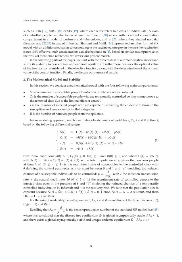
Math. Comput. Appl. 2018, 23, 64
such as SEIR [17], SIRS [18], or SIS [19], where each letter refers to a class of individuals. A classof controlled people can also be considered, as done in [20] where authors added a vaccinationcompartment in a model of pertussis and tuberculosis, and in [21] where they studied nonfataldiseases, and [22,23] in case of influenza. Sharomi and Malik [24] represented an other form of SIRmodel with an additional equation corresponding to the vaccinated category in the case the vaccinationis not 100% effective; such considerations can also be found in [4]. Based on similar assumptions as inthe two last mentioned references, we devise our present model.
In the following parts of the paper, we start with the presentation of our mathematical model andstudy its stability in cases of free and endemic equilibria. Furthermore, we seek the optimal valueof the free horizon considered in the objective function, along with the determination of the optimalvalue of the control function. Finally, we discuss our numerical results.
2. The Mathematical Model and Stability
In this section, we consider a mathematical model with the four following main compartments:
• S is the number of susceptible people to infection or who are not yet infected.• CS is the number of susceptible people who are temporarily controlled so they cannot move to
the removed class due to the limited effect of control.• I is the number of infected people who are capable of spreading the epidemic to those in the
susceptible and temporary controlled categories.• R is the number of removed people from the epidemic.
In our modeling approach, we choose to describe dynamics of variables S, CS, I and R at time t,based on the following differential system⎧⎪⎪⎪⎪⎪⎨⎪⎪⎪⎪⎪⎩
S(t) = Π(t)− βS(t)I(t)− aθS(t)− μS(t)
CS(t) = aθS(t)− bβCS(t)I(t)− μCS(t)
I(t) = β(S(t) + bCS(t))I(t)− γI(t)− μI(t)
R(t) = γI(t)− μR(t)
(1)
with initial conditions S(0) > 0, CS(0) ≥ 0, I(0) ≥ 0 and R(0) ≥ 0, and where Π(t) = μN(t),with N(t) = S(t) + CS(t) + I(t) + R(t) as the total population size, gives the newborn peopleat time t; aθ (0 ≤ a ≤ 1) is the recruitment rate of susceptibles to the controlled class withθ defining the control parameter as a constant between 0 and 1 and “a” modeling the reduced
chances of a susceptible individuals to be controlled; β =δ
N(t)with δ the infection transmission
rate, μ the natural death rate, bθ (0 ≤ b ≤ 1) the recruitment rate of controlled people to theinfected class even in the presence of θ and “b” modeling the reduced chances of a temporarilycontrolled individual to be infected; and γ is the recovery rate. We note that the population size isconstant because N(t) = S(t) + CS(t) + I(t) + R(t) = 0. Hence, N(t) = N = a constant, and then,Π(t) = Π = a constant.
For the sake of readability, hereafter, we use S, CS, I and R as notations of the time functions S(t),CS(t), I(t) and R(t).
Recalling that R0 =β
μ + γis the basic reproduction number of the standard SIR model (see [25]
where it is concluded that the disease free equilibrium E0 is global asymptotically stable if R0 ≤ 1,and there exists a global asymptotically stable and unique endemic equilibrium E+ if R0 > 1).
54

Math. Comput. Appl. 2018, 23, 64
Since the two first equations are independent of the last equation, we only study the stability ofthe following differential system⎧⎪⎪⎨⎪⎪⎩
S = Π − βSI − aθS − μS
CS = aθS − bβCS I − μCS
I = β(S + bCS)I − γI − μI
(2)
A disease free equilibrium in our case can be defined as E0 = (S0, C0S, 0) where S0 and C0
S areobtained based on the assumptions S = 0 and I = 0 when there is no infection.
Explicitly, we have S = 0 when I = 0, gives S0 =Π
μ + aθ. In addition, we have CS = 0 when
I = 0, gives C0S =
aθΠμ(μ + aθ)
.
If limt→+∞ CS(t) = 0 as a consequence of the case when θ = 0, we define the basic reproductionnumber for our case by RC
0 which is the average new infections produced by one infected individualduring his life cycle when the population is at E0.
Since I is the only infected compartment, then RC0 = β(S0 + bC0
S)×1
μ + γ. Thus, we have
RC0 =
βΠ(μ + aθ)(μ + γ)
+abβθΠ
μ(μ + aθ)(μ + γ)=
βΠ(μ + abθ)
μ(μ + aθ)(μ + γ)(3)
Now, we try to find the components of the endemic equilibrium E+ = (S+, C+S , I+) where S+
and C+S are obtained based on the assumptions S = 0 and CS = 0 when there is an infection.
Explicitly, we have S = 0 when I > 0, which gives S+ =Π
μ + aθ + βI+. In addition, we have
CS = 0 when I > 0, which gives C+S =
aθS+
μ + bβI+.
On the other part, we have I = 0 when I > 0, which gives
βS+ I+ + bβC+S I+ − γI+ − μI+ = 0
⇒ βΠ
μ + aθ + βI++ β
abθS+
μ + bβI+= γ + μ
⇒ βΠ(μ + bβI+) + abβθS+(μ + aθ + βI+) = (γ + μ)(μ + aθ + βI+)(μ + bβI+)
⇒ βΠ(μ + bβI+) + abβθΠ = (γ + μ)(μ + aθ + βI+)(μ + bβI+)
⇒ bβ2ΠI+ + βΠ(μ + abθ) = (γ + μ)(μ + aθ + βI+)(μ + bβI+)
⇒ (γ + μ)(μ + aθ)RC0 μ − (γ + μ)(aθμ + μ2)
= bβ2(γ + μ)I+2+ [(γ + μ)(βμ(1 + b) + abβθ)− bβ2Π]I+
Thus, we find that I+ is the root of the function f (I+) = α1 I+2+ α2 I+ + (1 − RC
0 )α3 where α1, α2
and α3 are constants.In the following three theorems, we state and prove stability results on free and endemic equilibria.
Theorem 1. E0 always exists and is locally asymptotically stable if RC0 < 1 (respectively, E0 is unstable
if RC0 > 1).
Proof. The existence of E0 is trivial.
55

Math. Comput. Appl. 2018, 23, 64
For the stability of E0, we define the Jacobian Matrix associated to the system in Equation (2) by⎛⎜⎝ −βI − aθ − μ 0 −βSaθ −bβI − μ −bβCSβI bβI β(S + bCS)− γ − μ
⎞⎟⎠ (4)
At E0, (4) becomes ⎛⎜⎝ −aθ − μ 0 −βS0
aθ −μ −bβC0S
0 0 β(S0 + bC0S)− γ − μ
⎞⎟⎠whose eigenvalues are
λ1 = −μ < 0,
λ2 = −(μ + aθ) < 0
λ3 = β(S0 + bβC0S)− γ − μ = (γ + μ)(RC
0 − 1),
which imply the local asymptotic stability of E0 when RC0 < 1, and its instability when RC
0 > 1.
Theorem 2. The differential system in Equation (2) admits E+ =
(Π
μ + aθ + βI+,
aθS+
μ + bβI+, I+
)as the
unique positive equilibrium and which is asymptotically stable when it exists, if and only if RC0 > 1.
Proof. First, we have
α1 = bβ2(γ + μ) > 0,
α2 = [(γ + μ)(βμ(1 + b) + abβθ)− bβ2Π],
α3 = μ(γ + μ)(μ + aθ) > 0
For the sufficiency of the existence and uniqueness of E+, so we have α1 > 0 and since f (0) =(1 − RC
0 )α3 < 0 if RC0 > 1, then f (I+) has two real roots, one is positive and the other is negative.
For the necessity, let us assume that RC0 ≤ 1 and prove that f (I+) has no positive roots. In this case,
the first fraction in Equation (3) verifies
βΠ ≤ (μ + γ)(μ + aθ)
⇒ α2 = (bβ(μ + aθ) + μβ)(γ + μ)− bβ2Π
≥ (bβ(μ + aθ) + μβ)(γ + μ)− bβ(μ + aθ)(μ + γ) = μβ(γ + μ) > 0.
Thus, we have α1 > 0 and since f (0) = (1− RC0 )α3 ≥ 0, f (I+) is increasing and f (I+) > f (0) ≥ 0,
then we reach the non-positivity of the roots.For the stability of E+, at E+, Equation (4) is defined as⎛⎜⎝ −βI+ − aθ − μ 0 −βS+
aθ −bβI+ − μ −bβC+S
βI+ bβI+ β(S+ + bC+S )− γ − μ
⎞⎟⎠
56

Math. Comput. Appl. 2018, 23, 64
=
⎛⎜⎜⎜⎜⎝− Π
S+0 −βS+
aθ − aθS+
C+S
−bβC+S
βI+ bβI+ 0
⎞⎟⎟⎟⎟⎠whose characteristic equation is λ3 + σ1λ2 + σ2λ + σ3 and where
σ1 =ΠS+
+aθS+
C+S
σ2 =aθΠC+
S+ b2β2C+
S I+ + β2S+ I+
σ3 = abβ2θS+ I+ +aθβ2S+2
I+
C+S
+b2β2ΠC+
S I+
S+.
Hence, we have
σ1σ2 − σ3
=ΠS+
(aθΠC+
S+ β2S+ I+
)
+aθS+
C+S
(aθΠC+
S+ b2β2C+
S I+)− abβ2θS+ I+
=aθΠ2
S+C+S+ (Π + aθ + βI+)β2S+ I+
+aθS+
C+S
(aθΠC+
S+ b2β2C+
S I+)− abβ2θS+ I+
=aθΠ2
S+C+S+ (Π + βI+)β2S+ I+ +
a2θ2ΠS+
C+2
S
+ aθS+ I+(β − bβ)2 + abβ2θS+ I+
> 0
Finally, based on the Routh–Hurwitz Criterion, we deduce the local asymptotic stability of E+.
Theorem 3. If RC0 ≤ 1, then E0 is globally asymptotically stable. If RC
0 > 1, then E+ is globallyasymptotically stable.
Proof. We suppose that RC0 ≤ 1 and we prove that E0 is globally asymptotically stable. Let us define
the Lyapunov function by
L0 = S − S0 − S0 lnSS0 + CS − C0
S − C0S ln
CS
C0S+ I.
Its derivative is then defined by
L0 = S + CS + I − S0 SS− C0
SCSCS
= Π − μS − μCS − μI − γI − S0 ΠS+ μS0 + βS0 I + aθS0 − C0
SaθSCS
+ bβC0S I + μC0
S.
57

Math. Comput. Appl. 2018, 23, 64
Since μ =aθS0
C0S
and Π = μS0 + aθS0, then this derivative becomes
L0 = −μS + 2μS0 + 3aθS0 − (μ + γ − βS0 − bβC0S)I
− aθC0SS
CS− S0
S(μS0 + aθS0)− aθS0CS
C0S
= −μS0(
SS0 +
S0
S− 2
)− aθS0
(CS
C0S+
S0
S+
C0SS
CSS0 − 3
)− (μ + γ)(1 − RC
0 )I
Now, we haveSS0 +
S0
S− 2 ≥ 0 and
CS
C0S+
S0
S+
C0SS
CSS0 − 3 ≥ 0 due to the fact that arithmetic
mean is larger than or equals to the geometric mean, and the equalities hold if S = S0 and CS = C0S.
Thus, L0 ≤ 0 which implies the global asymptotic stability of E0 based on Lyapunov–LaSalle’sinvariance principle.
Similarly, we study the global asymptotic stability of E+ by considering the followingLyapunov function
L+ = S − S+ − S+ lnS
S++ CS − C+
S − C+S ln
CS
C+S+ I − I+ − I+ ln
II+
.
The derivative is then defined as
˙L+ = S + CS + I − S+ SS− C+
SCSCS
− I+II
= Π − μS − μCS − (μ + γ)I − ΠS+
S+ μS+ + βS+ I + aθS+ − aθS
C+S
CS+ bβC+
S I + μC+S
− βSI+ − bβCS I+ + (μ + γ)I+
Since μ + γ = βS+ + bβC+S , μ =
aθS+ − bβC+S I+
C+S
and Π = μS+ + βS+ I+ + aθS+ = μS+ +
μC+S + (μ + γ)I+, this derivative becomes
˙L+ = 2Π − μS − aθS+ − bβC+S I+
C+S
CS − (μS+ + βI+S+ + aθS+)S+
S+ aθS+
− aθSC+
SCS
− βSI+ − bβCS I+
= 2(μS+ + βS+ I+ + aθS+)− μS − aθS+CS
C+S
+ aθS+ − μS+2
S− βS+2
I+
S
− aθS+2
S− aθSC+
SCS
− βSI+
= −(μS+ + βS+ I+)(
SS+
+S+
S− 2
)− aθS+
(CS
C+S+
S+
S+
C+S S
CSS+− 3
)≤ 0
58
Math. Comput. Appl. 2018, 23, 64
which is the final result, sought to prove for deducing that E+ is globally asymptotically stable.
3. Free Horizon Isoperimetric Optimal Control Approach
Now, we consider the mathematical model in Equation (1) with θ as a control function of time t.Motivated by the desire to find the optimal time needed to reduce the number of infected people
as much as possible while minimizing the value of the control θ(t) over a free (non-fixed) horizon t f ,our objective is to seek a couple (θ∗(t), t∗f ) such that
J(θ∗(t), t∗f ) = min(θ(t),t f )∈U×R+
J(θ(t), t f ) (5)
where J is the functional defined by
J(θ(t), t f ) = t2f +
∫ t f
0
(a′ I(t) + b′
2θ2(t)
)dt (6)
and where the control space U is defined by the set
U = {θ(t)|0 ≤ θ(t) ≤ 1, θ(t) measurable, t ∈ [0, t f ], t f f ree}
where a′ and b′ represent constant severity weights associated to functions I and θ, respectively.Alkama et al. treated three cases of the form of the free horizon t∗f in the final gain function of theirobjective function when applying a free final time optimal control approach to a cancer model [9].Here, we suppose that t∗f takes the quadratic form as formulated in Equation (6) to obtain a directformula which characterizes t∗f . In fact, if t∗f is taken linear or the final gain function is zero, t∗f wouldjust be approximated numerically due to the nature of necessary conditions in these two cases (see [9]for explanation).
Since managers of the anti-epidemic resources cannot well-predict whether their control strategywill reach the entire susceptible population over a fixed horizon T, we treat here an example wherethe number of targeted people in the susceptible class is equal for example to only a constantC = 3026 for T = 50 months. Hence, we try to find (θ∗(t), t∗f ) under the definition of the followingisoperimetric restriction
∫ T
0aθ(t)S(t)dt = C (7)
In [13], the authors defined an isoperimetric constraint on the control variable only to model thetotal tolerable dosage amount of a therapy along the treatment period. In their conferences talks [26,27],Kornienko et al. and De Pinho et al. introduced state constraints in an optimal control problem thatis subject to an S-Exposed-I-R differential system to model the situation of limited supply of vaccinebased on work in [14] and where the isoperimetric constraint is defined on the product of the controland state variables.
In our case, to take into account the constraint in Equation (7) for the resolution of the optimalcontrol problem in Equation (5), we consider a new variable Z defined as
Z(t) =∫ t
0aθ(v)S(v)dv (8)
59
Math. Comput. Appl. 2018, 23, 64
Then, we have Z(t) = aθ(t)S(t). Using notations of the state variables in the previous sectionand keeping θ as a notation of θ(t) and Z in place of Z(t), we study the differential system definedas follows ⎧⎪⎪⎪⎪⎪⎪⎪⎪⎨⎪⎪⎪⎪⎪⎪⎪⎪⎩
S = Π − βSI − aθS − μS
CS = aθS − bβCS I − μCS
I = β(S + bCS)I − γI − μI
R = γI − μR
Z = aθS
(9)
instead of the model in Equation (1). We also note that, when the minimization problem in Equation (5)is under the constraint in Equation (7), the application of Pontryagin’s Maximum Principle would notbe appropriate for this case, but the new variable Z has the advantage to convert Equations (5)–(7) toa classical optimal control problem under one restriction which is the system in Equation (9) only [28].If we follow most optimal control approaches in the literature, the objective function in Equation (6) willbe defined over a fixed time interval. However, t∗f is free here, and, to find the optimal duration neededto control an epidemic, it would be advantageous to managers of medical or health resources to controlan epidemic before reaching the fixed time T for lesser costs. For this purpose, we need to assume that0 ≤ t∗f ≤ T to guarantee the sufficient condition for an optimal θ∗ in the case of a free horizon. This isbecause θ∗ exists for the minimization problem in Equation (5) when Equation (6) is defined over T basedon the verified properties of the sufficient conditions as stated in details in Theorem 4.1, pp. 68–69 of [29]and that can easily be verified for many examples as ours, and this implies in our case that the existenceof an optimal control θ∗ and associated optimal trajectories S∗, C∗
S, I∗, R∗ and Z∗ comes directly from theconvexity of the integrand term in Equation (6) with respect to the control θ and the Lipschitz propertiesof the state system with respect to state variables S, CS, I, R and Z. Then, it exists for any time in theinterval [0, T] including t∗f . As regard the necessary conditions, we state and prove the following theorem.
Theorem 4. If there exist optimal control u∗ and optimal horizon t∗f which minimize Equation (6) along with theoptimal solutions S∗, C∗
S, I∗ and R∗ associated to the differential system in Equation (9), then there exist adjointvariables λk, k = 1, 2, 3, 4, 5 as notations of λk(t) and which satisfy the following adjoint differential system⎧⎪⎪⎪⎪⎪⎪⎪⎪⎨⎪⎪⎪⎪⎪⎪⎪⎪⎩
λ1 = λ1(βI∗ + μ + aθ∗)− aλ2θ∗ − βλ3 I∗ − aθλ5
λ2 = λ2(bβI∗ + μ)− bλ3βI∗
λ3 = −a′ + λ1βS∗ + bλ2βC∗S − λ3(β(S∗ + bC∗
S)− μ − γ)− λ4γ
λ4 = λ4μ
λ5 = 0
(10)
with the transversality conditions λk(t∗f ) = 0, k = 1, 2, 3, 4 and λ5(t∗f ) = constant which should be determined.Furthermore, the sought optimal control is characterized by
θ∗ = min(
max(
0,aS∗(λ1 − λ2 − λ5)
b′
), 1)
(11)
while the sought optimal horizon is characterized by
t∗f = −H(t∗f , S(t∗f ), CS(t∗f ), I(t∗f ), R(t∗f ), Z(t∗f ), λ1(t∗f ), λ2(t∗f ), λ3(t∗f ), λ4(t∗f ), λ5(t∗f ), θ(t∗f ))
2(12)
where H(t∗f , S(t∗f ), CS(t∗f ), I(t∗f ), R(t∗f ), Z(t∗f ), λ1(t∗f ), λ2(t∗f ), λ3(t∗f ), λ4(t∗f ), λ5(t∗f ), θ(t∗f )) defines theHamiltonian function as the sum of the integrand term of Equation (6) and the term λ1S + λ2CS + λ3 I +λ4R + λ5Z at t∗f .
60

Math. Comput. Appl. 2018, 23, 64
Moreover, t∗f is positive only when H(t∗f , S(t∗f ), CS(t∗f ), I(t∗f ), R(t∗f ), Z(t∗f ), λ1(t∗f ), λ2(t∗f ), λ3(t∗f ),λ4(t∗f ), λ5(t∗f ), θ(t∗f )) is negative.
Proof. Let H be a notation of the Hamiltonian function H(t, S(t), CS(t), I(t), R(t), Z(t), λ1(t), λ2(t),λ3(t), λ4(t), λ5(t), θ(t)) in all time t. Then, we have
H = a′ I + b′
2θ2 + λ1S + λ2CS + λ3 I + λ4R + λ5Z
= a′ I + b′
2θ2 + λ1(Π − βSI − aθS − μS) + λ2(aθS − bβCS I − μCS)
+λ3(β(S + bCS)I − γI − μI) + λ4(γI − μR) + aθSλ5
Using Pontryagin’s maximum principle [30], we have
λ1 = −∂H∂S
= λ1(βI∗ + μ + aθ∗)− aλ2θ∗ − βλ3 I∗ − aθλ5
λ2 = − ∂H∂CS
= λ2(bβI∗ + μ)− bλ3βI∗
λ3 = −∂H∂I
= −a′ + λ1βS∗ + bλ2βC∗S − λ3(β(S∗ + bC∗
S)− μ − γ)− λ4γ
λ4 = −∂H∂R
= λ4μ
λ5 = −∂H∂R
= 0
while the transversality conditions defined as minus the derivative of the final gain function withrespect to the state variables S, CS, I and R. Since the final gain function in Equation (6) does notcontain any term of these variables, then λk(t∗f ) = 0, k = 1, 2, 3, 4 and λ5(t∗f ) is unknown but we
are sure it is a constant since λ5(t) = 0 ∀t ∈ [0, t∗f ]. The solution of this problem is treated in thenext section.
The optimality condition at θ = θ∗ implies that∂H∂θ
= 0. Then, after setting S = S∗, we have
b′θ − aSλ1 + aSλ2 + aSλ5 = 0 ⇒ θ =aS(λ1 − λ2 − λ5)
b′
Taking into account the bounds of the control, we obtain,
θ∗ = min(
max(
0,aS∗(λ1 − λ2 − λ5)
b′
), 1)
Now, let us prove the necessary conditions on t∗f . As J(θ, t f ) reaches its minimum at θ∗ and t∗f ,we have
limh �→0
J(
θ∗, t∗f + h)− J
(θ∗, t∗f
)h
= 0
61

Math. Comput. Appl. 2018, 23, 64
with the consideration of the final gain function φ that we deduce it is defined in Equation (6) byφ(t f , S(t f ), CS(t f ), I(t f ), R(t f ), Z(t f )) = t2
f , while setting θ = θ∗ and t f = t∗f , we obtain
limh �→0
1h
⎡⎢⎣φ(t f + h, S(t f + h), CS(t f + h), I(t f + h), R(t f + h), Z(t f + h)) +
t f +h∫0
(aI(t) +
b2
θ2(t))
dt
−φ(t f , S(t f ), CS(t f ), I(t f ), R(t f ), Z(t f ))−t f∫
0
kI
(aI(t) +
b2
θ2(t))
dt
⎤⎥⎦ = 0
⇒ limh �→0
[φ(t f + h, S(t f + h), CS(t f + h), I(t f + h), R(t f + h), Z(t f + h))− φ(t f , S(t f ), CS(t f ), I(t f ), R(t f ), Z(t f ))
h
+1h
t f +h∫t f
(aI(t) +
b2
θ2(t))
dt
⎤⎥⎦ = 0
⇒ ∂φ
∂t(t f ) +
∂φ
∂S(t f )S(t f ) +
∂φ
∂CS(t f )CS(t f ) +
∂φ
∂I(t f ) I(t f ) +
∂φ
∂R(t f )R(t f ) +
∂φ
∂Z(t f )Z(t f ) + aI(t) +
b2
θ2(t) = 0
⇒ 2t f + H(t f , S(t f ), CS(t f ), I(t f ), R(t f ), Z(t f ), λ1(t f ), λ2(t f ), λ3(t f ), λ4(t f ), λ5(t f ), θ(t f )) = 0
⇒ t f +H(t f , S(t f ), CS(t f ), I(t f ), R(t f ), Z(t f ), λ1(t f ), λ2(t f ), λ3(t f ), λ4(t f ), λ5(t f ), θ(t f ))
2= 0
Finally, we have
t f = −H(t f , S(t f ), CS(t f ), I(t f ), R(t f ), Z(t f ), λ1(t f ), λ2(t f ), λ3(t f ), λ4(t f ), λ5(t f ), θ(t f ))
2
Otherwise, the positivity of t∗f under the condition of negativity of
H(t∗f , S(t∗f ), CS(t∗f ), I(t∗f ), R(t∗f ), Z(t∗f ), λ1(t∗f ), λ2(t∗f ), λ3(t∗f ), λ4(t∗f ), λ5(t∗f ), θ(t∗f ))
is trivial, but this is not a condition we should have necessarily for θ∗ since the Hamiltonian couldchange signs any time along the interval of study.
4. Numerical Simulations
Based on the formulation of Equation (8), we have Z(0) = 0 and Z(t f ) = C. Since the optimalcontrol problem consists to resolve the two-point boundary value problem defined by the two systemsin Equations (2) and (10), the differential system in Equation (2) will be numerically resolved forward intime because of its initial conditions and the value of Z(0) does not change, while the differential systemin Equation (10) will be numerically resolved backward in time because of its final or transversalityconditions but with the condition that Z(t f ) varies depending on the value of k. Based on the numericalapproach in [13], we propose also here to define a real function g such that k → g(k) = Z f − Zf andwhere Z f is the value of Z at t f for various values of k and Zf is the value fixed by C. This leadsto the combination of the Forward–Backward–Sweep Method (FBSM) which resolves the two-pointboundary value problem in Equations (2)–(10), with the secant-method to find the value of the root ′k′
of the function g [31]. The necessary condition on t∗f defined by the characterization in Equation (12),which leads to seek a fixed point of a real function F such that F(t∗f ) = t∗f . We choose to solve thisnumerical problem differently to the method used in [8,9] using the fixed point method. In brief,the four steps of numerical calculus associated to the resolution of our free optimal control problem (5)under isoperimetric constraint (7), are described in Algorithm 1.
62

Math. Comput. Appl. 2018, 23, 64
Algorithm 1: Resolution steps of the two-point boundary value optimal control problem (9) and (10).Step 0:
Guess an initial estimation to θ and t f inal .Step 1:
Use the initial condition S(0), CS(0), I(0), R(0) and Z(0) and the stocked values by θ andt f .
Find the optimal states S∗, C∗S, I∗, R∗ and Z∗ which iterate forward in the two-point
boundary value problem (2)–(10).Step 2:
Use the stocked values by θ and the transversality conditions λk(t f ) for k = 1, 2, 3, 4 whilesearching the constant λ5(t f ) using the secant-method.
Find the adjoint variables λk for k = 1, 2, 3, 4, 5 which iterate backward in the two-pointboundary value problem (2)–(10).
Step 3:
Update the control utilizing new S, CS, I, R, Z and λk for k = 1, 2, 3, 4, 5 in thecharacterization of θ∗ as presented in (11) while searching the optimal time t∗f characterizedby (12) using the fixed point method.
Step 4:
Test the convergence. If the values of the sought variables in this iteration and the finaliteration are sufficiently small, check out the recent values as solutions. If the values are notsmall, go back to Step 1.
Figure 1 depicts the SCS IRZ dynamics in the absence and presence of the control and we cansee that the number of susceptible people has increased linearly from its initial condition to a numberhigher than 92.5 individuals when we choose θ = 0, while the optimal state S∗ increases during thefirst months of the optimal control strategy and it decreases when we work with the characterization ofEquation (11). Simultaneously, the number of removed people increases to only a value close to eightpeople while it reaches a value higher than this number with a maximal peak equaling to 17 when θ = 0.As regards to the number of infected people, it decreases from its initial condition to a value close toan important value of 30 individuals because of the natural death and recovery only, while it decreasestowards a value very close to zero after the introduction of the control θ. We can see the relationshipbetween the number of controlled people and the optimal values taken by θ so when this is increasing,the optimal state C∗
S is also increasing. In fact, we can deduce that, with only small values of θ, we reachour goal by minimizing I function, and maximizing R function while the total number of the susceptiblewho received the control along T and which is represented by the function Z has not exceeded theimposed constant C. The dashed lines introduced in this figure show the highest fixed point valueof the sought final time, and we can understand that, at this point, we have already reached our goalwhich concerns the minimization of the number of infected people and maximization of the number ofremoved people. The next figure gives more information about the obtained value of t∗f .
63

Math. Comput. Appl. 2018, 23, 64
0 10 20 30 40 5060
70
80
90
when θ=0
time (in months)
S
0 10 20 30 40 5060
70
80
90
when θ≠0
time (in months)
S
0 10 20 30 40 500
5
10
15
20when θ=0
time (in months)
R
0 10 20 30 40 500
5
10
15
20when θ≠0
time (in months)
R
0 10 20 30 40 5025
30
35
40when θ=0
time (in months)
I
0 10 20 30 40 500
10
20
30
40when θ≠0
time (in months)
I
0 10 20 30 40 500
20
40
60
80number of controlled people
time (in months)C
S
0 10 20 30 40 500.8
0.82
0.84
0.86
0.88
0.9
0.92
0.94
0.96
0.98
1
the optimal control
time (in months)
θ*
0 5 10 15 20 25 30 35 40 45 500
2000
4000
time (in months)
Z
C=3026
Figure 1. SCS IRZ dynamics in the absence and presence of the control in the two cases θ = 0 and θ = 0.Parameters values: Π = 6.45, a = 0.06, b = 0.001, β = 0.0003, and μ = 0.05, γ = 0.1. Initial conditions:S(0) = 89, CS(0) = 0, I(0) = 40, and R(0) = 0. Severity weights constants: a′ = 1 and b′ = 50.
In Figure 2, we present dynamics of the functions S, I and R, and we can see the fixed points t∗f inthe first plot above. The solution of the equation F(t∗f ) = t∗f starts from an initial guess which equalszero, and increases to values that are very close or sometimes equal to 26 months (we note that, even ifthey appeared taking the value 26, this is not the case at all iterations but just because all values are veryclose to 26 with a small precision of about 10−4). As noted in this figure, for instance, the highest valueof t∗f = 26.4081 found at iteration 292 among 1000. In the same figure, in the plot below, we observethat, at t∗f indicated by the dashed purple line, the number of infected people has already taken thedirection towards zero values, while the number of removed people has already reached its positivepeak and started to decrease because of the decrease of the optimal control function θ∗, as shown in theprevious figure. This means that there is no need in this case to extend the optimal control approachfor other months since, at t∗f , Equation (5) has been almost realized.
64

Math. Comput. Appl. 2018, 23, 64
0 5 10 15 20 25 30 35 40 45 500
10
20
30
40
50
60
70
80
90
time (in months)
0 100 200 300 400 500 600 700 800 900 10000
5
10
15
20
25
30
Fixed points satisfying tf*=F(t
f*) with F(t
f*)=−H(t
f*)/2
Optimization steps
All
poss
ible
val
ues
of t f*
SIR
highest value is 26.4081 (found at iteration 292)
Figure 2. SIR dynamics with the precision of the optimal horizon t∗f with the same parameters, initialconditions and severity weights constants as in Figure 1.
In Figure 3, the fixed points t∗f for different values of the control severity weight b′ suggest that,as the value of b′ increases, t∗f increases. In fact, the bigger is b′, the lesser is the optimal control θ∗,which is important, as we can deduce from the formulation in Equation (11), and this is reasonablesince, when θ∗ is small, we need more time to control the epidemic. The obtained results in this figurecan be summarized as follows:
• When b′ = 60: I(t∗f ) = 6.734 with θ(t∗f ) = 0.8658 (iteration 278), which implies that 83.165% ofinfected people have left the I compartment.
• When b′ = 70: I(t∗f ) = 6.0627 with θ(t∗f ) = 0.8624 (iteration 295), which implies that 84.84325% ofinfected people have left the I compartment.
• When b′ = 80: I(t∗f ) = 4.7619 with θ(t∗f ) = 0.8573 (iteration 332), which implies that 88.09525% ofinfected people have left the I compartment.
65

Math. Comput. Appl. 2018, 23, 64
0 200 400 600 800 10000
5
10
15
20
25
30
35
40
45
Fixed points satisfying tf*=F(t
f*) with F(t
f*)=−H(t
f*)/2
Optimization steps
All
poss
ible
val
ues
of t f*
b’=60b’=70b’=80
highest value= 42.3728 (found at iteration 332)
highest value= 37.051 (found at iteration 295)
highest value= 31.9294 (found at iteration 278)
Figure 3. t∗f for different values of b′ with the same parameters, initial conditions and severity weightsconstants as in Figure 1.
In Figure 4, we show the impact of the initial condition of I function, namely I0, on fixed points t∗f ,and we can deduce from the obtained optimal horizons that, as I0 increases, t∗f increases, and thisis reasonable since, when the number of infected people is important, the anti-epidemic measuresneed longer time for controlling the situation. The obtained results in this figure can be summarizedas follows:
• When I(0) = 50: I(t∗f ) = 8.4416 with θ(t∗f ) = 0.8758 (iteration 278), which implies that 83.1168%of infected people have left the I compartment.
• When I(0) = 60: I(t∗f ) = 5.7018 with θ(t∗f ) = 0.8662 (iteration 338), which implies that 90.497% ofinfected people have left the I compartment.
• When I(0) = 70: I(t∗f ) = 8.1909 with θ(t∗f ) = 0.8802 (iteration 310), which implies that 88.2987%of infected people have left the I compartment.
66

Math. Comput. Appl. 2018, 23, 64
0 200 400 600 800 10000
5
10
15
20
25
30
35
Fixed points satisfying tf*=F(t
f*) with F(t
f*)=−H(t
f*)/2
Optimization steps
All
poss
ible
val
ues
of t f*
I(0)=50I(0)=60I(0)=70
highest value= 34.1597 (found at iteration 310)
highest value= 32.8953 (found at iteration 338)
highest value= 31.7294 (found at iteration 278)
Figure 4. t∗f for different values of the initial condition I(0) with the same parameters, severity weightsconstants and , initial conditions for S(0), CS(0), and R(0) as in Figure 1.
5. Conclusions
In this paper, we have determined the optimal duration needed for controlling an epidemic basedon a free horizon optimal control approach with an isoperimetric constraint and which has been appliedto a four-compartmental epidemic model where it is supposed that the controlled population doesnot reach the removed class due to the temporary effect of the control. The isoperimetric restrictionwhich has been proposed to define the number of susceptible people who receive the control along theanti-epidemic measures period, allowed us to find the optimal horizon of the optimal control strategywhen there are limited resources devised to fight against a disease. In the numerical simulations,we used the fixed point method since the necessary condition on the free horizon led to a fixed pointequation. Our results prove their usefulness, since, at the obtained optimal horizons for differentvalues of parameters and initial conditions on infection, the infected population size has been reducedand this presents an advantage of the followed control approach to managers of the health resourceseven when these are limited.
67

Math. Comput. Appl. 2018, 23, 64
Author Contributions: All authors contributed equally to this work. All authors read and approved the finalmanuscript.
Acknowledgments: The authors would like to thank all Managing Editors and members of the Editorial Boardwho were responsible for dealing with this paper, and the anonymous referees for their valuable comments andsuggestions, improving the content of this paper.
Conflicts of Interest: The authors declare no conflict of interest.
References
1. Zakary, O.; Rachik, M.; Elmouki, I. On the impact of awareness programs in HIV/AIDS prevention: An SIRmodel with optimal control. Int. J. Comput. Appl. 2016, 133, 1–6. [CrossRef]
2. Zakary, O.; Larrache, A.; Rachik, M.; Elmouki, I. Effect of awareness programs and travel-blocking operationsin the control of HIV/AIDS outbreaks: A multi-domains SIR model. Adv. Differ Equ. 2016, 2016, 169.[CrossRef]
3. Roy, P.K.; Saha, S.; Al Basir, F. Effect of awareness programs in controlling the disease HIV/AIDS: An optimalcontrol theoretic approach. Adv. Differ. Equ. 2015, 2015, 217. [CrossRef]
4. Rodrigues, H.S.; Monteiro, M.T.T.; Torres, D.F. Vaccination models and optimal control strategies to dengue.Math. Biosci. 2014, 247, 1–12. [CrossRef] [PubMed]
5. Kumar, A.; Srivastava, P.K. Vaccination and treatment as control interventions in an infectious disease modelwith their cost optimization. Commun. Nonlinear Sci. Numer. Simul. 2017, 44, 334–343. [CrossRef]
6. Liu, X.; Takeuchi, Y.; Iwami, S. SVIR epidemic models with vaccination strategies. J. Theor. Biol. 2008, 253, 1–11.[CrossRef] [PubMed]
7. Nainggolan, J.; Supian, S.; Supriatna, A.K.; Anggriani, N. Mathematical model of tuberculosis transmissionwith reccurent infection and vaccination. J. Phys. Conf. Ser. 2013, 423, 012059. [CrossRef]
8. Zakary, O.; Rachik, M.; Elmouki, I. How much time is sufficient for benefiting of awareness programsin epidemics prevention? A free final time optimal control approach. Int. J. Adv. Appl. Math. Mech.2017, 4, 26–40.
9. Alkama, M.; Larrache, A.; Rachik, M.; Elmouki, I. Optimal duration and dosage of BCG intravesicalimmunotherapy: A free final time optimal control approach. Math. Methods Appl. Sci. 2018, 41, 2209–2219.[CrossRef]
10. Zhou, L.; Fan, M. Dynamics of an SIR epidemic model with limited medical resources revisited. Nonlinear Anal.Real World Appl. 2012, 13, 312–324. [CrossRef]
11. Abdelrazec, A.; Bélair, J.; Shan, C.; Zhu, H. Modeling the spread and control of dengue with limited publichealth resources. Math. Biosci. 2016, 271, 136–145. [CrossRef] [PubMed]
12. Yu, T.; Cao, D.; Liu, S. Epidemic model with group mixing: Stability and optimal control based on limitedvaccination resources. Commun. Nonlinear Sci. Numer. Simul. 2018, 61, 54–70. [CrossRef]
13. Elmouki, I.; Saadi, S. BCG immunotherapy optimization on an isoperimetric optimal control problem for thetreatment of superficial bladder cancer. Int. J. Dyn. Control 2016, 4, 339–345. [CrossRef]
14. Neilan, R.M.; Lenhart, S. An Introduction to Optimal Control with an Application in Disease Modeling.In Modeling Paradigms and Analysis of Disease Trasmission Models; Gumel, A.B., Lenhart, S., Eds.; AmericanMathematical Society: Providence, RI, USA, 2010; pp. 67–82.
15. El Kihal, F.; Abouelkheir, I.; Rachik, M.; Elmouki, I. Optimal Control and Computational Method for theResolution of Isoperimetric Problem in a Discrete-Time SIRS System. Math. Comput. Appl. 2018, 23, 52.[CrossRef]
16. Kermack, W.O.; McKendrick, A.G. A Contribution to the Mathematical Theory of Epidemics. Proc. R. Soc. A1927, 115, 700–721. [CrossRef]
17. Korobeinikov, A. Lyapunov functions and global properties for SEIR and SEIS epidemic models. Math. Med.Biol. J. IMA 2004, 21, 75–83. [CrossRef]
18. Gonçalves, S.; Abramson, G.; Gomes, M.F. Oscillations in SIRS model with distributed delays. Eur. Phys. J. B2011, 81, 363. [CrossRef]
19. Gray, A.; Greenhalgh, D.; Mao, X.; Pan, J. The SIS epidemic model with Markovian switching. J. Math.Anal. Appl. 2012, 394, 496–516. [CrossRef]
68

Math. Comput. Appl. 2018, 23, 64
20. Kribs-Zaleta, C.M.; Velasco-Hernández, J.X. A simple vaccination model with multiple endemic states.Math. Biosci. 2000, 164, 183–201. [CrossRef]
21. Kribs-Zaleta, C.M.; Martcheva, M. Vaccination strategies and backward bifurcation in an age-since-infectionstructured model. Math. Biosci. 2002, 177, 317–332. [CrossRef]
22. Alexander, M.E.; Bowman, C.; Moghadas, S.M.; Summers, R.; Gumel, A.B.; Sahai, B.M. A vaccination modelfor transmission dynamics of influenza. SIAM J. Appl. Dyn. Syst. 2004, 3, 503–524. [CrossRef]
23. Shim, E. A note on epidemic models with infective immigrants and vaccination. Math. Biosci. Eng. 2006, 3, 557.[CrossRef] [PubMed]
24. Sharomi, O.; Malik, T. Optimal control in epidemiology. Ann. Oper. Res. 2017, 251, 55–71. [CrossRef]25. Hethcote, H.W. The mathematics of infectious diseases. SIAM Rev. 2000, 42, 599–653. [CrossRef]26. Kornienko, I.; Paiva, L.T.; De Pinho, M.D.R. Introducing state constraints in optimal control for health
problems. Procedia Technol. 2014, 17, 415–422. [CrossRef]27. De Pinho, M.D.R.; Kornienko, I.; Maurer, H. Optimal Control of a SEIR Model with Mixed Constraints
and L1 Cost. In Proceedings of the 11th Portuguese Conference on Automatic Control, Porto, Portugal,21–23 July 2014; pp. 135–145.
28. Lenhart, S.; Workman, J.T. Optimal Control Applied to Biological Models; CRC Press: New York, NY, USA, 2007.29. Fleming, W.H.; Rishel, R.W. Deterministic and Stochastic Optimal Control; Springer Science & Business Media:
New York, NY, USA, 2012.30. Pontryagin, L.S. Mathematical Theory of Optimal Processes; CRC Press: New York, NY, USA, 1987.31. Gumel, A.B.; Lenhart, S. Modeling Paradigms and Analysis of Disease Transmission Models; American
Mathematical Society: Providence, RI, USA, 2010.
c© 2018 by the authors. Licensee MDPI, Basel, Switzerland. This article is an open accessarticle distributed under the terms and conditions of the Creative Commons Attribution(CC BY) license (http://creativecommons.org/licenses/by/4.0/).
69

Mathematical
and Computational
Applications
Article
Optimal Strategies for Psoriasis Treatment
Ellina Grigorieva 1,* and Evgenii Khailov 2
1 TWU Department of Mathematics and Computer Science, Texas Woman’s University, Denton,TX 76204, USA
2 MSU Faculty of Computational Mathematics and Cybernetics, Lomonosov Moscow State University,Moscow 119992, Russia; [email protected]
* Correspondence: [email protected] or [email protected]; Tel.: +1-940-898-2452
Received: 1 August 2018; Accepted: 31 August 2018; Published: 4 September 2018
Abstract: Within a given time interval we consider a nonlinear system of differential equations describingpsoriasis treatment. Its phase variables define the concentrations of T-lymphocytes, keratinocytes anddendritic cells. Two scalar bounded controls are introduced into this system to reflect medication dosagesaimed at suppressing interactions between T-lymphocytes and keratinocytes, and between T-lymphocytesand dendritic cells. For such a controlled system, a minimization problem of the concentration ofkeratinocytes at the terminal time is considered. For its analysis, the Pontryagin maximum principle isapplied. As a result of this analysis, the properties of the optimal controls and their possible types areestablished. It is shown that each of these controls is either a bang-bang type on the entire time interval or(in addition to bang-bang type) contains a singular arc. The obtained analytical results are confirmed bynumerical calculations using the software “BOCOP-2.0.5”. Their detailed analysis and the correspondingconclusions are presented.
Keywords: psoriasis; nonlinear control system; optimal control; Pontryagin maximum principle;switching function; Lie brackets; singular arc; chattering control
1. Introduction
Psoriasis is an immune-mediated inflammatory skin disease that affects 2–3% of the populationaround the world [1]. The most characteristic features of the pathology are hyperproliferation and disruptedepidermal differentiation, altered immunological and vascular skin profiles. Manifestations of psoriasis canvary according to severity: from weak, when only a few characteristic psoriatic plaques are present on thebody of patients, to extremely severe ones, when the lesion affects almost the entire surface of the body andjoints. Disease can significantly reduce the standard of living and performance of patients [2]. There areestablished links between psoriasis and other diseases: obesity, diabetes, cardiovascular diseases, metabolicsyndrome, and depression [3]. Molecular-genetic causes of the disease are still not fully established.At the same time, various polymorphisms associated with psoriasis as well as several environmentalfactors that can lead to the manifestation of this disease are identified [4]. To date, about 150 million peoplearound the world are suffering from psoriasis. In the USA the annual cost of treatment is about $12 billion,while the existing therapies can only relieve symptoms and increase remission time. In addition, recentstudies have revealed the division of psoriasis into subtypes, depending on which patients may responddifferently to therapy. In some cases, despite costly and prolonged treatment, the patient’s condition maynot improve [5]. In recent years, studies have greatly expanded the understanding of the pathogenesis ofpsoriasis and allowed the development of numerous therapies.
In psoriasis, mathematical models are effectively used to predict cellular behavior of the skin inboth normal and pathological conditions. Among all possible models [6], we highlight the models thatare described by systems of differential equations [6–15]. In turn, controlled mathematical models areused to simulate the use of medication and dosage regimen, compare the effects of various drugs on
Math. Comput. Appl. 2018, 23, 45; doi:10.3390/mca23030045 www.mdpi.com/journal/mca70

Math. Comput. Appl. 2018, 23, 45
the affected areas of the skin, and to determine the most effective methods of treatment. Within theframework of a specific model, optimal control theory is used to find the best strategies in one sense oranother for psoriasis treatment.
For mathematical models of psoriasis treatment, optimal control problems were considered in [15–17],where the optimal treatment strategies minimizing the weighted sum of the total concentration ofkeratinocytes and the total cost of the treatment were found numerically. This cost of psoriasistreatment was expressed by an integral of the square of control, and these models were described usingsystems of differential equations linear in control. After applying the Pontryagin maximum principleas a necessary optimality condition, the corresponding optimal control problems were reduced totwo-point boundary value problems for the maximum principle, which were then solved numerically,applying standard mathematical software. This was because the right-hand sides of the systems ofdifferential equations of such boundary value problems were Lipschitz functions of the phase andadjoint variables.
In the optimal control problems for mathematical models of diseases and the spread of epidemics,the total cost of treatment can also be expressed by an integral of control [18–21]. In this case, the modelsare still described by systems of differential equations that are linear in control. Then, as shownin [21,22], after applying the Pontryagin maximum principle to such problems, the correspondingoptimal controls can contain singular arcs on which these controls are not uniquely determined fromthe maximum condition. After the existence of such singular arcs are established on appropriatesingular intervals, the corresponding optimality conditions are checked, and the concatenations ofsingular and nonsingular intervals are found, the finding of specific optimal solutions in optimalcontrol problems is still performed only numerically. This paper shows that optimal controls cancontain singular arcs in the minimization problem for the mathematical model of psoriasis treatmenteven in the absence of the controls in the integral terms of the functional to be minimized responsiblefor the cost of this treatment.
This paper is organized as follows. Section 2 is devoted to the description of the mathematicalmodel of psoriasis treatment and the formulation of the corresponding optimal control problem for it.Namely, we consider a nonlinear controlled system of three differential equations that presents theprocess of treating this disease. Its phase variables determine the concentrations of T-lymphocytes,keratinocytes, and dendritic cells. The interaction of these types of cells leads to the appearanceand development of psoriasis. There are two scalar bounded controls in the system that reflect alltypes of psoriasis treatment: skin creams that prevent or inhibit the formation, development andspread of psoriatic skin lesions, as well as pills and injections, also aimed at achieving similar results.At the same time, skin creams suppress the interaction between T-lymphocytes and keratinocytes;pills and injections weaken the interaction between T-lymphocytes and dendritic cells. All suchmedications are aimed at achieving the main goal, which is to reduce the number of keratinocytes.Therefore, for such a controlled system, at a given time interval the problem of minimizing theconcentration of keratinocytes at the end of the time interval is stated. An optimal solution for such aproblem, consisting of the optimal controls and the corresponding optimal solutions of the system,is analyzed using the Pontryagin maximum principle. Its application to the considered minimizationproblem is discussed in Section 3. Here, also possible types of the optimal controls are discussed:whether they are only bang-bang functions, or they can contain singular arcs in addition to thebang-bang intervals. A detailed analysis of the behavior of the optimal controls is given in Section 4.Here, we study the properties of the corresponding switching functions, which are crucial in suchanalysis. Using the Lie brackets of the geometric control theory allows us to obtain the Cauchyproblem for the switching functions. Such a Cauchy problem makes it possible to draw the conclusionsabout possible singular arcs of the optimal controls. The first one shows that these controls do notsimultaneously have singular arcs on the same singular intervals. The second of them is that when oneoptimal control has a singular arc on some singular interval, the second optimal control is constant onthis interval and takes one of its boundary values. The next two sections, Sections 5 and 6, are devoted
71

Math. Comput. Appl. 2018, 23, 45
to a detailed analysis of singular arcs of each optimal control. In these sections it is shown that oneof them can have a singular arc of the order of two, and the other can contain a singular arc of orderone. Also, for each of these singular arcs the corresponding necessary optimality conditions arechecked (Kelly-Cope-Moyer condition and Kelly condition). Finally, the forms of concatenations of thesingular arcs of the optimal controls with nonsingular intervals on which such controls are bang-bangfunctions are considered. Since, as previously mentioned, after discussing all such issues, finding thespecific optimal solutions is carried out numerically, then in Section 7 the results of the correspondingnumerical calculations and their discussion are presented. Section 8 contains our conclusions.
2. Mathematical Model and Optimal Control Problem
Let a time interval [0, T] be given, which is the period of psoriasis treatment. We consider onthis interval a mathematical model that establishes the links between the concentrations l(t), k(t),m(t) of T-lymphocytes, keratinocytes, and dendritic cells, respectively, because interactions betweenthese types of cells cause a disease such as psoriasis. Such a model is the nonlinear system ofdifferential equations:⎧⎪⎨⎪⎩
l′(t) = σ − δv(t)l(t)m(t)− γ1u(t)l(t)k(t)− μl(t),k′(t) = (β + δ)v(t)l(t)m(t) + γ2u(t)l(t)k(t)− λk(t),m′(t) = ρ − βv(t)l(t)m(t)− νm(t),
(1)
with given initial values:
l(0) = l0, k(0) = k0, m(0) = m0; l0, m0, k0 > 0. (2)
In System (1) we suppose that σ is the constant rate of accumulation for T-lymphocytes andρ is the constant accumulation rate of dendritic cells. The rate of activation of T-lymphocytes bydendritic cells is δ and β is the activation rate of dendritic cells by T-lymphocytes. Also, we considerthat the removal rates of T-lymphocytes, keratinocytes and dendritic cells are denoted by μ, λ and ν,respectively. Finally, we suppose that γ1 is the rate of activation of keratinocytes by T-lymphocytesand growth of keratinocytes due to T-lymphocytes occurs at the rate γ2.
Next, in System (1) two control functions u(t) and v(t) are introduced. The control u(t) is at theplaces of interaction between T-lymphocytes and keratinocytes and reflects the medication dosageto restrict the excessive growth of keratinocytes. In a similar way, the control v(t) is at the placesof interaction between T-lymphocytes and dendritic cells and reflects the medication dosage for therestriction of the excessive growth of keratinocytes as well. The controls u(t) and v(t) subject to thefollowing restrictions:
0 < umin ≤ u(t) ≤ 1, 0 < vmin ≤ v(t) ≤ 1. (3)
We consider that the set of all admissible controls Ω(T) is formed by all possible pairs of Lebesguemeasurable functions (u(t), v(t)), which for almost all t ∈ [0, T] satisfy Inequality (3).
Let us introduce a region:
Λ ={(l, k, m)� ∈ R3 : l > 0, k > 0, m > 0, l + k + m < M
},
where M is a positive constant that depends on the parameters σ, ρ, β, δ, μ, λ, ν, γ1, γ2 of System (1)and its initial values l0, k0, m0 from (2). Here R3 is the Euclidean space consisting of all column vectorsand the sign � means transposition.
Then, the boundedness, positiveness, and continuation of the solutions for System (1) is stated bythe following lemma.
72
Math. Comput. Appl. 2018, 23, 45
Lemma 1. Let the inclusion (l0, k0, m0)� ∈ Λ be valid. Then, for any pair of admissible controls
(u(t), v(t)) the corresponding absolutely continuous solutions l(t), k(t), m(t) for System (1) are definedon the entire interval [0, T] and satisfy the inclusion:
(l(t), k(t), m(t))� ∈ Λ, t ∈ (0, T]. (4)
Remark 1. Relationship (4) implies that the region Λ is a positive invariant set for System (1). The proof ofLemma 1 is fairly straightforward, and we omit it. Proofs of such statements are given, for example, in [16,23,24].
Now, let us consider for System (1) on the set of admissible controls Ω(T) the followingminimization problem:
J(u(·), v(·)) = k(T) → min(u(·),v(·))∈Ω(T)
, (5)
which consists in minimizing the concentration of keratinocites at the final moment T of psoriasistreatment. As already noted in [25], the optimal control problem (5) differs from problems thatare typically considered in the literature on the control of psoriasis models [15–17,26] in that thefunctional from (5) does not include an integral of the weighted sum of the squares of the controlsu(t) and v(t), which is responsible for the total cost of drug dosages. In psoriasis treatment, in mostcases, either a skin cream, or an oral medication are used. Both prescribed medications have regulardaily dosage and are not as harmful for patients as the drugs used in chemotherapy for cancertreatment [21]. Therefore, the total cost of psoriasis treatment in the meaning “harm” to a patient andthat usually mathematically is described by an integral of the weighted sum of the squares of thecontrols, can be ignored. Moreover, using the terminal functional from (5) instead of correspondingintegral functional [15–17,26] simplifies the subsequent analytical arguments.
The existence in the minimization problem (5) of the optimal controls (u∗(t), v∗(t)) and thecorresponding optimal solutions l∗(t), k∗(t), m∗(t) for System (1) follows from Lemma 1 andTheorem 4 ([27], Chapter 4).
Finally, based on the results from [17,23,26], we assume that the following assumption is true.
Assumption 1. Let the inequalities:
γ1 = γ2, (β + δ)γ1 > δγ2, λ > μ, λ > ν (6)
be valid.
Let us introduce the constants:
α = γ1γ−12 (β + δ)− δ, ε = α(λ − ν) + δ(λ − μ).
By this assumption, it is easy to see that these constants are positive.
3. Pontryagin Maximum Principle
We apply the Pontryagin maximum principle [28] to analyze the optimal controls u∗(t), v∗(t) andthe corresponding optimal solutions l∗(t), k∗(t), m∗(t). Firstly, let us define the Hamiltonian:
H(l, m, k, u, v,ψ1, ψ2, ψ3) = (σ − δvlm − γ1ulk − μl)ψ1
+ ((β + δ)vlm + γ2ulk − λk)ψ2 + (ρ − βvlm − νm)ψ3,
where ψ1, ψ2, ψ3 are the adjoint variables.
73

Math. Comput. Appl. 2018, 23, 45
Secondly, we calculate the required partial derivatives:
H′l (l, m, k, u, v, ψ1, ψ2, ψ3) = uk(γ2ψ2 − γ1ψ1)
+ vm(−δψ1 + (β + δ)ψ2 − βψ3)− μψ1,
H′k(l, m, k, u, v, ψ1, ψ2, ψ3) = ul(γ2ψ2 − γ1ψ1)− λψ2,
H′m(l, m, k, u, v, ψ1, ψ2, ψ3) = vl(−δψ1 + (β + δ)ψ2 − βψ3)− νψ3,
H′u(l, m, k, u, v, ψ1, ψ2, ψ3) = lk(γ2ψ2 − γ1ψ1),
H′v(l, m, k, u, v, ψ1, ψ2, ψ3) = lm(−δψ1 + (β + δ)ψ2 − βψ3).
Then, in accordance with the Pontryagin maximum principle, for the optimal controlsu∗(t), v∗(t) and the optimal solutions l∗(t), k∗(t), m∗(t) there exists a vector-function ψ∗(t) =
(ψ∗1 (t), ψ∗
2 (t), ψ∗3 (t))
� such that:
• ψ∗(t) is a nontrivial solution of the adjoint system:⎧⎪⎪⎪⎪⎪⎨⎪⎪⎪⎪⎪⎩
ψ∗1′(t) = −u∗(t)k∗(t)(γ2ψ∗
2 (t)− γ1ψ∗1 (t))
−v∗(t)m∗(t)(−δψ∗1 (t) + (β + δ)ψ∗
2 (t)− βψ∗3 (t)) + μψ∗
1 (t),ψ∗
2′(t) = −u∗(t)l∗(t)(γ2ψ∗
2 (t)− γ1ψ∗1 (t)) + λψ∗
2 (t),ψ∗
3′(t) = −v∗(t)l∗(t)(−δψ∗
1 (t) + (β + δ)ψ∗2 (t)− βψ∗
3 (t)) + νψ∗3 (t),
ψ∗1 (T) = 0, ψ∗
2 (T) = −1, ψ∗3 (T) = 0;
(7)
• the controls u∗(t) and v∗(t) maximize the Hamiltonian
H(l∗(t), k∗(t), m∗(t), u, v, ψ∗1 (t), ψ∗
2 (t), ψ∗3 (t))
with respect to variables u ∈ [umin, 1] and v ∈ [vmin, 1] for almost all t ∈ [0, T], and therefore theysatisfy the relationships:
u∗(t) =
⎧⎪⎨⎪⎩1 , if Lu(t) > 0,any u ∈ [umin, 1] , if Lu(t) = 0,umin , if Lu(t) < 0;
(8)
v∗(t) =
⎧⎪⎨⎪⎩1 , if Lv(t) > 0,any v ∈ [vmin, 1] , if Lv(t) = 0,vmin , if Lv(t) < 0;
(9)
where the functions:
Lu(t) = l∗(t)k∗(t)(γ2ψ∗2 (t)− γ1ψ∗
1 (t)),Lv(t) = l∗(t)m∗(t)(−δψ∗
1 (t) + (β + δ)ψ∗2 (t)− βψ∗
3 (t))(10)
are the switching functions describing the behavior of the controls u∗(t) and v∗(t) in accordancewith Formulas (8) and (9), respectively.
Analysis of Formulas (8) and (9) shows possible types of the optimal controls u∗(t) and v∗(t).They can only have a bang-bang type and switch between the corresponding values umin and 1,vmin and 1. This occurs, when passing through the points at which the switching functions Lu(t) andLv(t) are zero, the sign of these functions changes. Or, in addition to intervals of a bang-bang type,the controls u∗(t) and v∗(t) can also contain singular arcs [22,29]. This occurs when the switchingfunctions Lu(t) and Lv(t) individually or both simultaneously vanish identically on certain subintervalsof the interval [0, T]. Furthermore, such subintervals we will call as singular intervals. The followingsections are devoted to a detailed study of singular arcs for the optimal controls u∗(t) and v∗(t).
74
Math. Comput. Appl. 2018, 23, 45
Now, we establish the important property of the controls u∗(t) and v∗(t). Namely, by Lemma 1,the initial values of System (7), Formula (10), and the continuity of the switching functions Lu(t) andLv(t), the following lemma is valid.
Lemma 2. There exist such values tu� , tv
� ∈ [0, T) that the inequalities Lu(t) < 0 and Lv(t) < 0 hold for all tfrom the corresponding intervals (tu
� , T] and (tv�, T].
Corollary 1. Lemma 2 and Formulas (8) and (9) imply the following relationships for the optimal controlsu∗(t) and v∗(t):
u∗(t) = umin, t ∈ (tu� , T]; v∗(t) = vmin, t ∈ (tv
�, T].
4. Differential Equations of the Switching Functions
Let us obtain differential equations for the switching functions Lu(t) and Lv(t). To do this,we draw on the concepts and notations of geometric control theory from [21,22].
Again, we consider the Euclidean space R3 in which the value 〈τ, s〉 is the scalar product of itselements. Let z = (l, k, m)� ∈ R3. Then, we rewrite System (1) as follows
z′(t) = f (z(t)) + u(t)g(z(t)) + v(t)h(z(t)), (11)
where
f (z) =
⎛⎜⎝ σ − μl−λk
ρ − νm
⎞⎟⎠ , g(z) =
⎛⎜⎝−γ1lkγ2lk
0
⎞⎟⎠ , h(z) =
⎛⎜⎝ −δlm(β + δ)lm−βlm
⎞⎟⎠ (12)
with f (z) the drift and g(z), h(z) the control vector fields of this system. Here z(t) is the column vectorconsisting of the solutions l(t), k(t), m(t) that correspond to the admissible controls u(t) and v(t),that is z(t) = (l(t), k(t), m(t))� ∈ R3. Let D f (z), Dg(z) and Dh(z) be the Jacobian matrices of thevector functions f (z), g(z) and h(z), respectively. By Formula (12), we find the following relationships:
D f (z) =
⎛⎜⎝−μ 0 00 −λ 00 0 −ν
⎞⎟⎠ , Dg(z) =
⎛⎜⎝−γ1k −γ1l 0γ2k γ2l 0
0 0 0
⎞⎟⎠ ,
Dh(z) =
⎛⎜⎝ −δm 0 −δl(β + δ)m 0 (β + δ)l−βm 0 −βl
⎞⎟⎠ .
(13)
Then, using the introduced concepts and notations, it is easy to see that z∗(t) =
(l∗(t), k∗(t), m∗(t))� is the optimal trajectory for System (11) corresponding to the optimal controlsu∗(t) and v∗(t); ψ∗(t) = (ψ∗
1 (t), ψ∗2 (t), ψ∗
3 (t))� is the appropriate nontrivial solution for the adjoint
System (7), or in the new notations:⎧⎨⎩ ψ′∗(t) = −(
D f (z∗(t)) + u∗(t)Dg(z∗(t) + v∗(t)Dh(z∗(t)))�
ψ∗(t),ψ∗(T) = (0,−1, 0)�.
(14)
The Hamiltonian
H(t) = H(l∗(t), k∗(t), m∗(t), u∗(t), v∗(t), ψ∗1 (t), ψ∗
2 (t), ψ∗3 (t))
takes the form:
H(t) = 〈ψ∗(t), f (z∗(t))〉+ u∗(t)〈ψ∗(t), g(z∗(t))〉+ v∗(t)〈ψ∗(t), h(z∗(t))〉.
75

Math. Comput. Appl. 2018, 23, 45
The switching functions Lu(t) and Lv(t), defined by Formula (10), become the scalar products ofthe adjoint function ψ∗(t) with the corresponding control fields g(z∗(t)) and h(z∗(t)):
Lu(t) = 〈ψ∗(t), g(z∗(t))〉, Lv(t) = 〈ψ∗(t), h(z∗(t))〉. (15)
Now, according to [21,22], we introduce for the drift and control vector fields f (z), g(z) and h(z)the corresponding Lie brackets:
[ f , g](z) = Dg(z) f (z)− D f (z)g(z), (16)
[ f , h](z) = Dh(z) f (z)− D f (z)h(z), (17)
[g, h](z) = Dh(z)g(z)− Dg(z)h(z). (18)
Using (11) and (14)–(18), the derivatives of the switching functions Lu(t) and Lv(t) can be obtainedas follows
L′u(t) = 〈ψ∗(t), [ f , g](z∗(t))〉+ v∗(t)〈ψ∗(t), [h, g](z∗(t))〉, (19)
L′v(t) = 〈ψ∗(t), [ f , h](z∗(t))〉+ u∗(t)〈ψ∗(t), [g, h](z∗(t))〉. (20)
Now, using (12) and (13) in (16)–(18), we compute the Lie brackets [ f , g](z), [ f , h](z) and [g, h](z).As a result, we find the formulas:
[ f , g](z) =
⎛⎜⎝−γ1k(σ − λl)γ2k(σ − μl)
0
⎞⎟⎠ , [g, h](z) =
⎛⎜⎝ γ1(β + δ)l2m−γ2(β + δ)l2m − αγ2lkm
γ1βlkm
⎞⎟⎠ ,
[ f , h](z) =
⎛⎜⎝ −δ((ρl + σm)− νlm)
(β + δ)((ρl + σm) + (λ − μ − ν)lm)
−β((ρl + σm)− μlm)
⎞⎟⎠ .
(21)
Let us write these Lie brackets in a more convenient form for the subsequent analysis. For this,we introduce the following linearly independent vectors:
p =
⎛⎜⎝−γ1
γ2
0
⎞⎟⎠ , q =
⎛⎜⎝ −δ
β + δ
−β
⎞⎟⎠ , r =
⎛⎜⎝100
⎞⎟⎠ .
It is easy to see that the following representations for the control vector fields g(z) and h(z)are valid:
g(z) = lk · p, h(z) = lm · q.
Using these relationships, Formula (15) for the switching functions Lu(t) and Lv(t) can berewritten as
Lu(t) = l∗(t)k∗(t)〈ψ∗(t), p〉, Lv(t) = l∗(t)m∗(t)〈ψ∗(t), q〉. (22)
Now, let us find the decompositions of the Lie brackets [ f , g](z), [ f , h](z) and [g, h](z),defined by (21), by the vectors p, q, r. As a result, we have the representations:
[ f , g](z) = k(σ − μl) · p + γ1(λ − μ)lk · r, (23)
[ f , h](z) = γ−12 (β + δ)(λ − ν)lm · p + (ρl + σm − μlm) · q + εlm · r, (24)
[g, h](z) = −lm((β + δ)l − δk) · p − γ1lkm · q. (25)
76

Math. Comput. Appl. 2018, 23, 45
Next, let us introduce the auxiliary function G(t) = 〈ψ∗(t), r〉 = ψ∗1 (t), and define the following
absolutely continuous functions:
au(t) = l−1∗ (t)(σ − μl∗(t)), av(t) = γ−12 (β + δ)(λ − ν)k−1∗ (t)m∗(t),
bv(t) = l−1∗ (t)m−1∗ (t)(ρl∗(t) + σm∗(t)− μl∗(t)m∗(t)),cu(t) = γ1(λ − μ)l∗(t)k∗(t), cv(t) = εl∗(t)m∗(t),d(t) = k−1∗ (t)m∗(t)((β + δ)l∗(t)− δk∗(t)), e(t) = γ1k∗(t).
(26)
It is easy to see that the functions cu(t) and cv(t) are positive on the interval [0, T].Finally, substituting (23)–(25) into (19), (20) and using (22), (26), we find the required differential
equations for the switching functions Lu(t) and Lv(t):
L′u(t) = au(t)Lu(t) + cu(t)G(t) + v∗(t)(d(t)Lu(t) + e(t)Lv(t)),
L′v(t) = av(t)Lu(t) + bv(t)Lv(t) + cv(t)G(t)
− u∗(t)(d(t)Lu(t) + e(t)Lv(t)).
We add to these equations the first equation of System (7), written with use of the functions Lu(t),Lv(t), G(t):
G′(t) = −u∗(t)l−1∗ (t)Lu(t)− v∗(t)l−1∗ (t)Lv(t) + μG(t),
as well as the corresponding initial values:
Lu(T) = −γ2l∗(T)k∗(T), Lv(T) = −(β + δ)l∗(T)m∗(T), G(T) = 0.
As a result, we obtain the Cauchy problem for the switching functions Lu(t), Lv(t) and thefunction G(t): ⎧⎪⎪⎪⎪⎪⎨⎪⎪⎪⎪⎪⎩
L′u(t) = au(t)Lu(t) + cu(t)G(t) + v∗(t)(d(t)Lu(t) + e(t)Lv(t)),
L′v(t) = av(t)Lu(t) + bv(t)Lv(t) + cv(t)G(t)
−u∗(t)(d(t)Lu(t) + e(t)Lv(t)),G′(t) = −u∗(t)l−1∗ (t)Lu(t)− v∗(t)l−1∗ (t)Lv(t) + μG(t),Lu(T) = −γ2l∗(T)k∗(T), Lv(T) = −(β + δ)l∗(T)m∗(T), G(T) = 0,
(27)
which we will use to justify the properties of the functions Lu(t) and Lv(t).Now, let us establish the properties of the switching functions Lu(t) and Lv(t).
Firstly, the following lemma is true.
Lemma 3. There is no subinterval of the interval [0, T] at which both switching functions Lu(t) and Lv(t) areidentically zero.
Proof of Lemma 3. We suppose the contrary. Let there be the interval Δu,v ⊂ [0, T] on which thefunctions Lu(t) and Lv(t) identically equal to zero. Then, their derivatives L′
u(t) and L′v(t) almost
everywhere on this subinterval also vanish. From the first two differential equations of the Cauchyproblem (27) we find that G(t) = 0 everywhere on the subinterval Δu,v. Hence, on this subinterval thederivative G′(t) is almost everywhere zero. Therefore, the third differential equation of the Cauchyproblem (27) is also satisfied. Using the definition of the function G(t), Lemma 1 and Formula (10),we find that the adjoint function ψ∗(t) vanishes identically on the subinterval Δu,v. Since the system oflinear differential equations (7) is homogeneous, then ψ∗(t) = 0 identically everywhere on the interval[0, T], which is contradictory. Hence, our assumption was wrong, and the subinterval Δu,v ⊂ [0, T] onwhich both switching functions Lu(t) and Lv(t) are identically zero, does not exist. This completesthe proof.
77

Math. Comput. Appl. 2018, 23, 45
Secondly, the following lemma holds.
Lemma 4. Let the subinterval Δu ⊂ [0, T] be a singular interval of the optimal control u∗(t).Then, everywhere on this subinterval, the optimal control v∗(t) is constant and takes one of the values {vmin; 1}.
Proof of Lemma 4. On the subinterval Δu the switching function Lu(t) is identically zero, and itsderivative L′
u(t) vanishes almost everywhere on this interval. Then, the first differential equation ofthe Cauchy problem (27) yields the equality:
cu(t)G(t) + v∗(t)e(t)Lv(t) = 0, t ∈ Δu. (28)
Let us suppose that the switching function Lv(t) is zero at some point tu0 ∈ Δu, that is
Lv(tu0 ) = 0. (29)
Then, (28) implies the equality:G(tu
0 ) = 0. (30)
The identical equality to zero of the function Lu(t) on the subinterval Δu and (29), (30) leadus to the equality ψ∗(tu
0 ) = 0. A further repetition of the corresponding arguments from Lemma 3gives a contradiction. Hence, our assumption was wrong, and the switching function Lv(t) doesnot vanish at any point of the subinterval Δu. Therefore, it is sign-definite on this subinterval,and, by Formula (9), the optimal control v∗(t) corresponding to it, is constant and takes one ofthe values {vmin; 1}. This completes the proof.
Furthermore, performing arguments similar to the arguments of Lemma 4, one can show that thefollowing lemma is valid.
Lemma 5. Let the subinterval Δv ⊂ [0, T] be a singular interval of the optimal control v∗(t).Then, everywhere on this subinterval, the optimal control u∗(t) is constant and takes one of the values {umin; 1}.
Now, we strengthen the result obtained in Lemma 4. Namely, the following lemma holds.
Lemma 6. Let the subinterval Δu = (tu1 , tu
2 ) ⊂ [0, T], where tu1 > 0, be a singular interval of the optimal
control u∗(t). Then, there exists a number εu > 0 such that on the interval (tu1 − εu, tu
2 + εu) the optimalcontrol v∗(t) is constant and takes one of the values {vmin; 1}.
Proof of Lemma 6. It suffices to show that the ends of the subinterval Δu = (tu1 , tu
2 ) cannot be zeros ofthe switching function Lv(t), which is an absolutely continuous function. Indeed, if such a fact holds,that is the inequalities:
Lv(tu1 ) = 0, Lv(tu
2 ) = 0
are true, then Lemma 6 immediately follows from the Theorem on the stability of the sign of acontinuous function [30]. Therefore, for definiteness, we consider the right end tu
2 of the subintervalΔu. Let us suppose the contrary. This means that the equality:
Lv(tu2 ) = 0 (31)
is valid. Then, for the function G(t) the following two cases are possible.Case 1. Let G(tu
2 ) = 0. The definition of the function G(t), Lemma 1 and the second formulaof (10) imply the relationship:
(β + δ)ψ∗2 (t
u2 ) = βψ∗
3 (tu2 ). (32)
78

Math. Comput. Appl. 2018, 23, 45
If ψ∗2 (t
u2 ) = 0, then (32) yields ψ∗
3 (tu2 ) = 0. This fact leads to contradictory equality ψ∗(tu
2 ) = 0,as the proofs of Lemmas 3 and 4 show. If ψ∗
2 (tu2 ) = 0, then again the definition of the function G(t),
Lemma 1 and the first formula of (10) imply Lu(tu2 ) = 0. The absolutely continuity of the function Lu(t)
and the Theorem on the stability of the sign of a continuous function [30] lead to the existence of a leftneighborhood of the point tu
2 at which the switching function Lu(t) is sign-definite. This contradictsthe fact that such a left neighborhood of the point tu
2 belongs to the subinterval Δu, which is a singularportion of the optimal control u∗(t). Thus, Case 1 is impossible.
Case 2. Let G(tu2 ) = 0. For definiteness, we consider that the inequality:
G(tu2 ) > 0 (33)
is true. As it was already noted, Lv(t) and G(t) are the absolutely continuous functions. In Lemma 4it was established that the control v∗(t) is constant on the subinterval Δu, that is v∗(t) = v∗.Therefore, by (31), (33) and the Theorem on the stability of the sign of a continuous function [30],there exists the interval (tu
2 , tu2 ) ⊂ Δu on which the inequality:
cu(t)G(t) + v∗e(t)Lv(t) > 0 (34)
is valid. Let tu0 be the midpoint of this interval. We rewrite the first differential equation from the
Cauchy problem (27) as
L′u(t) = (au(t) + v∗d(t))Lu(t) + (cu(t)G(t) + v∗e(t)Lv(t)).
Then, we integrate this equation on the interval (tu2 , tu
2 ) with the initial value Lu(tu0 ) = 0.
As a result, the following formula can be found:
Lu(t) =t∫
tu0
e
t∫s(au(ξ)+v∗d(ξ))dξ
(cu(s)G(s) + v∗e(s)Lv(s)) ds. (35)
By (34) and (35), we obtain the positivity of the function Lu(t) for t > tu0 and the negativity of this
function for t < tu0 on the interval (tu
2 , tu2 ). This is again contradictory. Hence, Case 2 is also impossible.
Thus, our assumption was wrong, and the switching function Lv(t) does not vanish at the pointtu2 . This completes the proof.
Furthermore, carrying out arguments similar to the arguments of Lemma 6, we can show that thefollowing lemma holds, which strengthens the result of Lemma 5.
Lemma 7. Let the subinterval Δv = (tv1, tv
2) ⊂ [0, T], where tv1 > 0, be a singular interval of the optimal
control v∗(t). Then, there exists a number εv > 0 such that on the interval (tv1 − εv, tv
2 + εv) the optimal controlu∗(t) is constant and takes one of the values {umin; 1}.
Remark 2. From Lemmas 4–7 we conclude that when a singular arc occurs for one of the optimal controls,u∗(t) or v∗(t), System (1) becomes on the corresponding singular interval a system with one control, becausethe other control is constant.
Next, in Sections 5 and 6, we separately study the existence of singular arcs of the optimalcontrols u∗(t) and v∗(t), applying the approach from [21]. It consists in the sequential differentiationon a singular interval of the corresponding switching function. We carry out this differentiationif the derivative of even order does not have a nonzero term containing control. If such a termappears in a second order derivative, then we say that a singular arc is of the order of one. If itoccurs in a derivative of the fourth order, then it is considered that the singular arc is of the order
79

Math. Comput. Appl. 2018, 23, 45
of two. Then, the corresponding optimality condition of a singular arc is checked. If it is satisfied,we find the formulas of the optimal control and the corresponding optimal solutions of System (1)on a singular interval corresponding to such a singular arc. Also, the type of concatenation of thissingular arc with non-singular intervals is studied, where the considered optimal control is bang-bang.Finally, we demonstrate a singular arc of the optimal control through the results of a numerical solutionof the minimization problem (5), presented in Section 7.
5. Investigation of a Singular Arc of the Optimal Control u*(t)
Let us study the existence of a singular arc of the optimal control u∗(t). According to [22,29],this means the existence of a subinterval Δu ⊂ [0, T] on which the corresponding switching functionLu(t) identically vanishes. By Lemma 4, everywhere on this subinterval the optimal control v∗(t) is aconstant function taking one of the values {vmin; 1}, that is,
v∗(t) = v∗ ∈ {vmin; 1}, t ∈ Δu.
Then, Formula (19) of the first derivative L(1)u (t) of the switching function Lu(t) is rewritten in
the form:L(1)
u (t) = 〈ψ∗(t), [ f + v∗h, g](z∗(t))〉, t ∈ Δu. (36)
Let us transform the right-hand side of this formula. To do this, we rewrite (23) and (25) as
[ f , g](z) = θ f ,g(z)p + χ f ,g(z)r, [h, g](z) = θh,g(z)p + ηh,g(z)q, (37)
whereθ f ,g(z) = (σ − μl)k, χ f ,g(z) = γ1(λ − μ)lk,
θh,g(z) = lm((β + δ)l − δk), ηh,g(z) = γ1lkm.
Then, using (37), we can write the Lie bracket [ f + v∗h, g](z) as follows
[ f + v∗h, g](z) = θu(z)p + ηu(z)q + χu(z)r, (38)
whereθu(z) = θ f ,g(z) + v∗θh,g(z) = (σ − μl)k + v∗lm((β + δ)l − δk),
ηu(z) = v∗ηh,g(z) = γ1v∗lkm,
χu(z) = χ f ,g(z) = γ1(λ − μ)lk.
Substituting (38) into the right-hand side of (36), we obtain the relationship:
L(1)u (t) = θu(z∗(t))〈ψ∗(t), p〉+ ηu(z∗(t))〈ψ∗(t), q〉+ χu(z∗(t))〈ψ∗(t), r〉, t ∈ Δu. (39)
Now, differentiating (36), we find the formula for the second derivative L(2)u (t) of the switching
function Lu(t):L(2)
u (t) = 〈ψ∗(t), [ f + v∗h, [ f + v∗h, g]](z∗(t))〉+ u∗(t)〈ψ∗(t), [g, [ f + v∗h, g]](z∗(t))〉, t ∈ Δu.
(40)
Let us transform the terms of this formula. First, we consider the second term and its factor
〈ψ∗(t), [g, [ f + v∗h, g]](z∗(t))〉. (41)
By analogy with (16)–(18), we have equality:
[g, [ f + v∗h, g]](z) = D[ f + v∗h, g](z)g(z)− Dg(z)[ f + v∗h, g](z), (42)
80

Math. Comput. Appl. 2018, 23, 45
where D[ f + v∗h, g](z) is the Jacobi matrix of the vector function [ f + v∗h, g](z). Using (38), we findthe relationship:
D[ f + v∗h, g](z) = D(θu(z)p) + D(ηu(z)q) + D(χu(z)r)
= p(∇θu(z))� + q(∇ηu(z))� + r(∇χu(z))�,(43)
where ∇θu(z), ∇ηu(z), ∇χu(z) are the column gradients of the functions θu(z), ηu(z), χu(z),respectively. In addition, the representations:
Dg(z) = p(τg(z))�, Dh(z) = q(τh(z))� (44)
are valid, where the vector functions τg(z), τh(z) are defined as
τg(z) =
⎛⎜⎝kl0
⎞⎟⎠ , τh(z) =
⎛⎜⎝m0l
⎞⎟⎠ .
We substitute (43) and the first representation of (44) into (42). After the necessary transformations,the following relationship can be obtained:
[g, [ f + v∗h, g]](z) =(〈∇θu(z), g(z)〉 − 〈[ f + v∗h, g](z), τg(z)〉
)p
+〈∇ηu(z), g(z)〉q + 〈∇χu(z), g(z)〉r.
Substituting this expression into (41), we find the formula:
〈ψ∗(t), [g,[ f + v∗h, g]](z∗(t))〉=(〈∇θu(z∗(t)), g(z∗(t))〉 − 〈[ f + v∗h, g](z∗(t)), τg(z∗(t))〉
)〈ψ∗(t), p〉
+ 〈∇ηu(z∗(t)), g(z∗(t))〉〈ψ∗(t), q〉+ 〈∇χu(z∗(t)), g(z∗(t))〉〈ψ∗(t), r〉.(45)
In (39) the function χu(z∗(t)) is positive on the interval [0, T]. Therefore, let us express the scalarproduct 〈ψ∗(t), r〉 through the remaining terms as follows
〈ψ∗(t), r〉 = χ−1u (z∗(t))L(1)
u (t)− χ−1u (z∗(t))θu(z∗(t))〈ψ∗(t), p〉
− χ−1u (z∗(t))ηu(z∗(t))〈ψ∗(t), q〉,
(46)
and then, we substitute this expression into (45). After the necessary transformations, the followingrelationship finally can be obtained:
〈ψ∗(t), [g, [ f + v∗h, g]](z∗(t))〉 = χ−1u (z∗(t))〈∇χu(z∗(t)), g(z∗(t))〉L(1)
u (t)
+ χ−1u (z∗(t))
{〈χu(z∗(t))∇θu(z∗(t))− θu(z∗(t))∇χu(z∗(t)), g(z∗(t))〉
− χu(z∗(t))〈[ f + v∗h, g](z∗(t)), τg(z∗(t))〉}〈ψ∗(t), p〉
+ χ−1u (z∗(t))〈χu(z∗(t))∇ηu(z∗(t))− ηu(z∗(t))∇χu(z∗(t)), g(z∗(t))〉〈ψ∗(t), q〉.
(47)
On the subinterval Δu the switching function Lu(t) vanishes identically, that is
Lu(t) = l∗(t)k∗(t)〈ψ∗(t), p〉 = 0, (48)
81

Math. Comput. Appl. 2018, 23, 45
and therefore its first derivative L(1)u (t) is also zero everywhere on this subinterval:
L(1)u (t) = 0. (49)
Then, Formula (47) is simplified and takes the following form:
〈ψ∗(t), [g, [ f + v∗h, g]](z∗(t))〉= χ−1
u (z∗(t))〈χu(z∗(t))∇ηu(z∗(t))− ηu(z∗(t))∇χu(z∗(t)), g(z∗(t))〉〈ψ∗(t), q〉. (50)
Let us calculate the right-hand side of this formula. For this, we consider the expression(χu(z)∇ηu(z)− ηu(z)∇χu(z)). Calculating the column gradients ∇ηu(z), ∇χu(z) of the correspondingfunctions ηu(z), χu(z), the following equality can be found:
χu(z)∇ηu(z)− ηu(z)∇χu(z) = γ1(λ − μ)v∗
⎛⎜⎝ 00
l2k2
⎞⎟⎠ . (51)
Multiplying this expression scalarly by the vector function g(z) from (12), we conclude that thescalar product
〈χu(z)∇ηu(z)− ηu(z)∇χu(z), g(z)〉is zero. Consequently, (50) has the form:
〈ψ∗(t), [g, [ f + v∗h, g]](z∗(t))〉 = 0, t ∈ Δu. (52)
Now, let us consider the first term on the right-hand side of (40):
〈ψ∗(t), [ f + v∗h, [ f + v∗h, g]](z∗(t))〉. (53)
By analogy with (42), we have the equality:
[ f + v∗h, [ f + v∗h, g]](z) = D[ f + v∗h, g](z)( f + v∗h)(z)− D( f + v∗h)(z)[ f + v∗h, g](z). (54)
Let us find the Jacobi matrix D( f + v∗h)(z). The Jacobi matrix Dh(z) of the vector function h(z) isgiven by the second formula of (44). The use of direct calculations allows us to find the representationof the Jacobi matrix D f (z) from (13) in the following form:
D f (z) = p
⎛⎜⎝ 0−γ−1
2 λ
−γ−12 β−1(β + δ)ν
⎞⎟⎠�
+ q
⎛⎜⎝ 00
β−1ν
⎞⎟⎠�
+ r
⎛⎜⎝ −μ
−γ1γ−12 λ
−β−1αν
⎞⎟⎠�
. (55)
Then, we obtain the required representation of the Jacobi matrix D( f + v∗h)(z) as
D( f + v∗h)(z) = p(τup )
� + q(τuq (z))
� + r(τur )
�, (56)
where
τup =
⎛⎜⎝ 0−γ−1
2 λ
−γ−12 β−1(β + δ)ν
⎞⎟⎠ , τuq (z) =
⎛⎜⎝ v∗m0
β−1ν + v∗l
⎞⎟⎠ , τur =
⎛⎜⎝ −μ
−γ1γ−12 λ
−β−1αν
⎞⎟⎠ .
82

Math. Comput. Appl. 2018, 23, 45
We substitute (43) and (56) into (54). After the necessary transformations, the following formulacan be found:
[ f + v∗h, [ f + v∗h, g]](z) =(〈∇θu(z), ( f + v∗h)(z)〉 − 〈[ f + v∗h, g](z), τu
p 〉)
p
+(〈∇ηu(z), ( f + v∗h)(z)〉 − 〈[ f + v∗h, g](z), τu
q (z)〉)
q
+(〈∇χu(z), ( f + v∗h)(z)〉 − 〈[ f + v∗h, g](z), τu
r 〉)
r.
Substituting this formula into (53), we obtain the expression:
〈ψ∗(t), [ f + v∗h, [ f + v∗h, g]](z∗(t))〉=(〈∇θu(z∗(t)), ( f + v∗h)(z∗(t))〉 − 〈[ f + v∗h, g](z∗(t)), τu
p 〉)〈ψ∗(t), p〉
+(〈∇ηu(z∗(t)), ( f + v∗h)(z∗(t))〉 − 〈[ f + v∗h, g](z∗(t)), τu
q (z∗(t))〉)〈ψ∗(t), q〉
+(〈∇χu(z∗(t)), ( f + v∗h)(z∗(t))〉 − 〈[ f + v∗h, g](z∗(t)), τu
r 〉)〈ψ∗(t), r〉.
(57)
Finally, let us substitute (46) into (57). After the necessary transformations, we find the relationship:
〈ψ∗(t), [ f + v∗h, [ f + v∗h, g]](z∗(t))〉= χ−1
u (z∗(t)){〈∇χu(z∗(t)), ( f + v∗h)(z∗(t))〉 − 〈[ f + v∗h, g](z∗(t)), τu
r 〉}
L(1)u (t)
+ χ−1u (z∗(t))
{〈χu(z∗(t))∇θu(z∗(t))− θu(z∗(t))∇χu(z∗(t)), ( f + v∗h)(z∗(t))〉
− 〈[ f + v∗h, g](z∗(t)), χu(z∗(t))τup − θu(z∗(t))τu
r 〉}〈ψ∗(t), p〉
+ χ−1u (z∗(t))
{〈χu(z∗(t))∇ηu(z∗(t))− ηu(z∗(t))∇χu(z∗(t)), ( f + v∗h)(z∗(t))〉
− 〈[ f + v∗h, g](z∗(t)), χu(z∗(t))τuq (z∗(t))− ηu(z∗(t))τu
r 〉}〈ψ∗(t), q〉.
(58)
On the subinterval Δu Equalities (48) and (49) are valid. Then, Formula (58) is simplified andtakes the following form:
〈ψ∗(t), [ f + v∗h, [ f + v∗h, g]](z∗(t))〉= χ−1
u (z∗(t)){〈χu(z∗(t))∇ηu(z∗(t))− ηu(z∗(t))∇χu(z∗(t)), ( f + v∗h)(z∗(t))〉
− 〈[ f + v∗h, g](z∗(t)), χu(z∗(t))τuq (z∗(t))− ηu(z∗(t))τu
r 〉}〈ψ∗(t), q〉.
(59)
Let us calculate the right-hand side of this formula. The expression (χu(z)∇ηu(z)− ηu(z)∇χu(z))is given by (51). Multiplying this expression scalarly by the vector function ( f + v∗h)(z), defined by thevector functions f (z) and h(z) from (12), we obtain the following formula for the first term in braces:
〈χu(z)∇ηu(z)− ηu(z)∇χu(z), ( f + v∗h)(z)〉= γ2
1(λ − μ)v∗l2k2(ρ − νm − βv∗lm).(60)
For the second term in braces, we first find the relationship:
χu(z)τuq (z)− ηu(z)τu
r = γ1lk
⎛⎜⎝ λv∗mγ1γ−1
2 λv∗mβ−1(λ − μ)ν + (λ − μ)v∗l + β−1ανv∗m
⎞⎟⎠ ,
83

Math. Comput. Appl. 2018, 23, 45
and then, by (38), obtain the representation:
[ f + v∗h, g](z) =
⎛⎜⎜⎝γ1
((σ − μl)k + v∗((β + δ)l − δk)lm
)+ γ1(λ − μ)lk − γ1δv∗lkm
γ2
((σ − μl)k + v∗((β + δ)l − δk)lm
)+ γ1(β + δ)v∗lkm
−γ1βv∗lkm
⎞⎟⎟⎠ .
Multiplying the last two expressions scalarly and taking into account (60), we have the followingexpression for the relationship in braces of (59):
− γ21v∗l2k2
(α(λ − ν)v∗m2 + λ(λ − μ)m − ρ(λ − μ)
). (61)
Let us define the quadratic function:
w2(m) = α(λ − ν)v∗m2 + λ(λ − μ)m − ρ(λ − μ).
We use this function, when substitute (61) together with the formula of the function χu(z) into (59).After the necessary transformations, this formula is written as follows
〈ψ∗(t), [ f + v∗h, [ f + v∗h, g]](z∗(t))〉= −γ1(λ − μ)−1v∗l∗(t)k∗(t)w2(m∗(t))〈ψ∗(t), q〉, t ∈ Δu.
(62)
Finally, let us substitute (52) and (62) into (40). As a result, we have the formula of the secondderivative L(2)
u (t) of the switching function Lu(t):
L(2)u (t) = −γ1(λ − μ)−1v∗l∗(t)k∗(t)w2(m∗(t))〈ψ∗(t), q〉, t ∈ Δu. (63)
On the subinterval Δu not only the switching function Lu(t) itself and its first derivative L(1)u (t)
vanish, but also the second derivative L(2)u (t). By Lemma 1, the linear independence of the vectors p, q,
r and the non-triviality of the adjoint function ψ∗(t), the relationship:
L(2)u (t) = 0, t ∈ Δu
implies equality:w2(m∗(t)) = 0, t ∈ Δu. (64)
By Assumption 1, the discriminant of the quadratic function w2(m) is positive, and w2(0) < 0,and therefore, it has a unique positive root msing, defined by the formula:
msing =−(λ − μ)λ +
√(λ − μ)2λ2 + 4αρv∗(λ − μ)(λ − ν)
2α(λ − ν)v∗.
This root is the value of the solution m∗(t) on the subinterval Δu. We note the important propertiesof the value msing:
msing ∈(
0, ρν−1)
, w′2(msing) > 0. (65)
Analyzing (63), we see that on the subinterval Δu the second derivative L(2)u (t) of the switching
function Lu(t) does not contain the control u∗(t). It means that the order of the singular arc is
84

Math. Comput. Appl. 2018, 23, 45
greater than one [22,29]. Therefore, we continue to differentiate the switching function Lu(t) on thissubinterval, and using (63) find its third derivative L(3)
u (t):
L(3)u (t) =− γ1(λ − μ)−1v∗
{l∗(t)k∗(t)w′
2(m∗(t))m′∗(t)〈ψ∗(t), q〉
+ w2(m∗(t))(
l∗(t)k∗(t)〈ψ∗(t), q〉)′}
.(66)
On the subinterval Δu Equality (64) is valid, and therefore the second term in braces of (66)is zero. Substituting the formula for m′∗(t) from System (1) into the first term of (66), we find therequired formula:
L(3)u (t) =− γ1(λ − μ)−1v∗l∗(t)k∗(t)w′
2(msing)
×(
ρ − νmsing − βv∗l∗(t)msing
)〈ψ∗(t), q〉, t ∈ Δu.
(67)
On the subinterval Δu the third derivative L(3)u (t) is also zero that leads to the equality:
m′∗(t) = 0. (68)
It allows us to find a value lsing that is the value of the solution l∗(t) on this subinterval:
lsing =ρ − νmsing
βv∗msing. (69)
We note that due to the inclusion of (65), the value lsing is positive.
Finally, on the subinterval Δu let us calculate the fourth derivative L(4)u (t) of the switching function
Lu(t) using (66). Some of the terms that are obtained with such a differentiation vanish by virtue of (64)and (68). As a result, the following relationship can be obtained:
L(4)u (t) = γ1(λ − μ)−1βv2∗lsingk∗(t)msingw′
2(msing)
×(
σ − μlsing − δv∗lsingmsing − γ1u∗(t)lsingk∗(t))〈ψ∗(t), q〉, t ∈ Δu,
(70)
which implies the expression:
∂
∂uL(4)
u (t) = −γ21(λ − μ)−1βv2∗l2
singk2∗(t)msingw′2(msing)〈ψ∗(t), q〉
= −γ21(λ − μ)−1βv2∗lsingk2∗(t)w′
2(msing)Lv(t), t ∈ Δu.(71)
Here we applied the second formula of (22). It is easy to see that this expression is sign-definiteeverywhere on the subinterval Δu. Therefore, firstly, the order of the singular arc equals two.Secondly, the necessary optimality condition of the singular arc, the Kelly-Cope-Moyer condition [29],is either carried out in a strengthened form, and then the singular arc exists, or it is not satisfied,and then the singular arc does not exist. By [29] and (71), the strengthened Kelly-Cope-Moyer conditionleads to the inequality:
γ21(λ − μ)−1βv2∗lsingk2∗(t)w′
2(msing)Lv(t) > 0, t ∈ Δu. (72)
By Assumption 1, Lemma 1, and the inequality of (65), Relationship (72) implies the inequalityLv(t) > 0, which in turn, by Formula (9), implies v∗ = 1 everywhere on the subinterval Δu.
85

Math. Comput. Appl. 2018, 23, 45
Remark 3. On the subinterval Δu ⊂ [0, T], which is the singular interval of the optimal control u∗(t),the optimal control v∗(t) is constant and takes the value 1. This leads to the corresponding correction of theformulations of Lemmas 4 and 6.
Next, Formula (70) and the vanishing of the fourth derivative L(4)u (t) of the switching function
Lu(t) yield the following relationship for the control using(t) and function ksing(t):
using(t)ksing(t) =σ − μlsing − δlsingmsing
γ1lsing, (73)
which are the control u∗(t) and solution k∗(t) on the subinterval Δu. Formula (69) allows us torewrite (73) as follows
using(t)ksing(t) =w4(msing)
γ1lsing, t ∈ Δu. (74)
Here w4(m) is the quadratic function given by the formula:
w4(m) = δνm2 + (σβ + νμ − δρ)m − μρ.
By the inclusion of (65), we consider this function on the interval[0, ρν−1]. The relationships:
w4(0) = −μρ < 0, w4
(ρν−1
)= ρν−1σβ > 0
lead to the conclusion that the function w4(m) has exactly one zero m� ∈(0, ρν−1). In turn, this fact
implies the validity of the formula:
w4(m)
⎧⎪⎨⎪⎩< 0 , if 0 ≤ m < m�,= 0 , if m = m�,> 0 , if m� < m ≤ ρν−1.
We apply this formula in analysis of (74). Positivity of the product on its left-hand side and theinclusion of (65) imply the validity of the inclusion:
msing ∈(
m�, ρν−1)
,
which is a necessary condition for the existence of the singular arc.Finally, let us discuss the behavior of the optimal control u∗(t) over the entire interval [0, T].
When the inclusion using(t) ∈ [umin, 1] holds for all t ∈ Δu, the control using(t) is admissible. Corollary 1shows that the singular arc of the optimal control u∗(t) is concatenated with the nonsingular interval,where this control is bang-bang. Let ξ ∈ (0, T) be the time moment, where such a concatenation occurs.Then, as it follows from [22,29], when using(t) ∈ (umin, 1) for all t ∈ Δu, the nonsingular intervalcontains at least the countable number of switchings of the control u∗(t), accumulating to the pointξ. This behavior of the optimal control u∗(t) on nonsingular intervals is called a chattering [22,29],and will be observed on both sides of the subinterval Δu.
Thus, the above arguments of this section lead us to the validity of the following proposition.
Proposition 1. The optimal control u∗(t) on a singular interval can contain a singular arc of order two,which concatenates with bang-bang intervals of this control using chattering. On such an interval the optimalcontrol v∗(t) is constant and takes the value 1.
86

Math. Comput. Appl. 2018, 23, 45
6. Investigation of a Singular Arc of the Optimal Control v∗(t)
Now, let us carry out arguments similar to those presented in the previous section to study theexistence of a singular arc for the optimal control v∗(t). According to [22,29], this means the existenceof a subinterval Δv ⊂ [0, T] on which the corresponding switching function Lv(t) identically vanishes.By Lemma 5, everywhere on this subinterval the optimal control u∗(t) is a constant function that takesone of the values {umin; 1}, that is,
u∗(t) = u∗ ∈ {umin; 1}, t ∈ Δv.
Then, Formula (20) for the first derivative L(1)v (t) of the switching function Lv(t) is rewritten in
the form:L(1)
v (t) = 〈ψ∗(t), [ f + u∗g, h](z∗(t))〉, t ∈ Δv. (75)
Let us transform the right-hand side of this formula. To do this, we rewrite (24) and (25) as
[ f , h](z) = θ f ,h(z)p + η f ,h(z)q + χ f ,h(z)r, [g, h](z) = θg,h(z)p + ηg,h(z)q, (76)
whereθ f ,h(z) = γ−1
2 (β + δ)(λ − ν)lm, η f ,h(z) = ρl + σm − μlm, χ f ,h(z) = εlm,
θg,h(z) = −θh,g(z) = −lm((β + δ)l − δk), ηg,h(z) = −ηh,g(z) = −γ1lkm.
Then, using (76), we can write the Lie bracket [ f + u∗g, h](z) as follows
[ f + u∗g, h](z) = θv(z)p + ηv(z)q + χv(z)r, (77)
whereθv(z) = θ f ,h(z) + u∗θg,h(z) = lm(γ−1
2 (β + δ)(λ − ν)− u∗((β + δ)l − δk)),
ηv(z) = η f ,h(z) + u∗ηg,h(z) = ρl + σm − μlm − γ1u∗lkm,
χv(z) = χ f ,h(z) = εlm.
Substituting (77) into the right-hand side of (75), we obtain the relationship:
L(1)v (t) = θv(z∗(t))〈ψ∗(t), p〉+ ηv(z∗(t))〈ψ∗(t), q〉+ χv(z∗(t))〈ψ∗(t), r〉, t ∈ Δv. (78)
Now, differentiating (75), we find the formula for the second derivative L(2)v (t) of the switching
function Lv(t):L(2)
v (t) = 〈ψ∗(t), [ f + u∗g, [ f + u∗g, h]](z∗(t))〉+ v∗(t)〈ψ∗(t), [h, [ f + u∗g, h]](z∗(t))〉, t ∈ Δv.
(79)
Let us transform the terms of this formula. First, we consider the second term and its factor
〈ψ∗(t), [h, [ f + u∗g, h]](z∗(t))〉. (80)
By analogy with (16)–(18), we have equality:
[h, [ f + u∗g, h]](z) = D[ f + u∗g, h](z)h(z)− Dh(z)[ f + u∗g, h](z), (81)
where D[ f + u∗g, h](z) is the Jacobi matrix of the vector function [ f + u∗g, h](z). Using (77), we findthe relationship:
D[ f + u∗g, h](z) = D(θv(z)p) + D(ηv(z)q) + D(χv(z)r)
= p(∇θv(z))� + q(∇ηv(z))� + r(∇χv(z))�,(82)
87

Math. Comput. Appl. 2018, 23, 45
where ∇θv(z), ∇ηv(z), ∇χv(z) are the column gradients of the functions θv(z), ηv(z), χv(z),respectively. We substitute expression (82) and the second representation of (44) into (81). After thenecessary transformations, the following relationship can be obtained:
[h, [ f + u∗g, h]](z) = 〈∇θv(z), h(z)〉p
+(〈∇ηv(z), h(z)〉 − 〈[ f + u∗g, h](z), τh(z)〉
)q + 〈∇χv(z), h(z)〉r.
Substituting this expression into (80), we find the formula:
〈ψ∗(t), [h, [ f + u∗g, h]](z∗(t))〉 = 〈∇θv(z∗(t)), h(z∗(t))〉〈ψ∗(t), p〉+(〈∇ηv(z∗(t)), h(z∗(t))〉 − 〈[ f + u∗g, h](z∗(t)), τh(z∗(t))〉
)〈ψ∗(t), q〉
+ 〈∇χv(z∗(t)), h(z∗(t))〉〈ψ∗(t), r〉.(83)
In (78), the function χv(z∗(t)) is positive on the interval [0, T]. Therefore, let us express the scalarproduct 〈ψ∗(t), r〉 through the remaining terms as follows
〈ψ∗(t), r〉 = χ−1v (z∗(t))L(1)
v (t)− χ−1v (z∗(t))θv(z∗(t))〈ψ∗(t), p〉
− χ−1v (z∗(t))ηv(z∗(t))〈ψ∗(t), q〉,
(84)
and then, we substitute this expression into (83). After the necessary transformations, the followingrelationship finally can be obtained:
〈ψ∗(t), [h, [ f + u∗g, h]](z∗(t))〉 = χ−1v (z∗(t))〈∇χv(z∗(t)), h(z∗(t))〉L(1)
v (t)
+ χ−1v (z∗(t))〈χv(z∗(t))∇θv(z∗(t))− θv(z∗(t))∇χv(z∗(t)), h(z∗(t))〉〈ψ∗(t), p〉
+ χ−1v (z∗(t))
{〈χv(z∗(t))∇ηv(z∗(t))− ηv(z∗(t))∇χv(z∗(t)), h(z∗(t))〉
− χv(z∗(t))〈[ f + u∗g, h](z∗(t)), τh(z∗(t))〉}〈ψ∗(t), q〉.
(85)
On the subinterval Δv the switching function Lv(t) vanishes identically, that is
Lv(t) = l∗(t)m∗(t)〈ψ∗(t), q〉 = 0, (86)
and therefore its first derivative L(1)v (t) is also zero everywhere on this subinterval:
L(1)v (t) = 0. (87)
Then, Formula (85) is simplified and takes the following form:
〈ψ∗(t), [h, [ f + u∗g, h]](z∗(t))〉= χ−1
v (z∗(t))〈χv(z∗(t))∇θv(z∗(t))− θv(z∗(t))∇χv(z∗(t)), h(z∗(t))〉〈ψ∗(t), p〉. (88)
Let us calculate the right-hand side of this formula. For this, we consider the expression(χv(z)∇θv(z)− θv(z)∇χv(z)). Calculating the column gradients ∇θv(z), ∇χv(z) of the correspondingfunctions θv(z), χv(z), the following equality can be found:
χv(z)∇θv(z)− θv(z)∇χv(z) = εu∗
⎛⎜⎝−(β + δ)l2m2
δl2m2
0
⎞⎟⎠ . (89)
88

Math. Comput. Appl. 2018, 23, 45
Multiplying this expression scalarly by the vector function h(z) from (12), we conclude that thefollowing relationship holds:
〈χv(z)∇θv(z)− θv(z)∇χv(z), h(z)〉 = 2εδ(β + δ)u∗l3m3.
Substituting this relationship together with the formula of the function χv(z) into (88), we seethat it has the form:
〈ψ∗(t), [h, [ f + u∗g, h]](z∗(t))〉 = 2δ(β + δ)u∗l2∗(t)m∗(t)2〈ψ∗(t), p〉, t ∈ Δv. (90)
Now, let us consider the first term on the right-hand side of (79):
〈ψ∗(t), [ f + u∗g, [ f + u∗g, h]](z∗(t))〉. (91)
By analogy with (81), we have the equality:
[ f + u∗g, [ f + u∗g, h]](z) = D[ f + u∗g, h](z)( f + u∗g)(z)− D( f + u∗g)(z)[ f + u∗g, h](z). (92)
Let us find the Jacobi matrix D( f + u∗g)(z). The Jacobi matrices D f (z) and Dg(z) of thecorresponding vector functions f (z) and g(z) from (12) are given by the representation (55) andthe first formula of (44). Then, the required representation can be written as
D( f + u∗g)(z) = p(τvp (z))
� + q(τvq )
� + r(τvr )
�, (93)
where
τvp (z) =
⎛⎜⎝ u∗k−γ−1
2 λ + u∗l−γ−1
2 β−1(β + δ)ν
⎞⎟⎠ , τvq =
⎛⎜⎝ 00
β−1ν
⎞⎟⎠ , τvr = τu
r =
⎛⎜⎝ −μ
−γ1γ−12 λ
−β−1αν
⎞⎟⎠ .
We substitute (82) and (93) into (92). After the necessary transformations, the following formulacan be found:
[ f + u∗g, [ f + u∗g, h]](z) =(〈∇θv(z), ( f + u∗g)(z)〉 − 〈[ f + u∗g, h](z), τv
p (z)〉)
p
+(〈∇ηv(z), ( f + u∗g)(z)〉 − 〈[ f + u∗g, h](z), τv
q 〉)
q
+(〈∇χv(z), ( f + u∗g)(z)〉 − 〈[ f + u∗g, h](z), τv
r 〉)
r.
Substituting this formula into (91), we obtain the expression:
〈ψ∗(t), [ f + u∗g, [ f + u∗g, h]](z∗(t))〉=(〈∇θv(z∗(t)), ( f + u∗g)(z∗(t))〉 − 〈[ f + u∗g, h](z∗(t)), τv
p (z∗(t))〉)〈ψ∗(t), p〉
+(〈∇ηv(z∗(t)), ( f + u∗g)(z∗(t))〉 − 〈[ f + u∗g, h](z∗(t)), τv
q 〉)〈ψ∗(t), q〉
+(〈∇χv(z∗(t)), ( f + u∗g)(z∗(t))〉 − 〈[ f + u∗g, h](z∗(t)), τv
r 〉)〈ψ∗(t), r〉.
(94)
89

Math. Comput. Appl. 2018, 23, 45
Now, let us substitute (84) into (94). After the necessary transformations, we have the relationship:
〈ψ∗(t), [ f + u∗g, [ f + u∗g, h]](z∗(t))〉= χ−1
v (z∗(t)){〈∇χv(z∗(t)), ( f + u∗g)(z∗(t))〉 − 〈[ f + u∗g, h](z∗(t)), τv
r 〉}
L(1)v (t)
+ χ−1v (z∗(t))
{〈χv(z∗(t))∇θv(z∗(t))− θv(z∗(t))∇χv(z∗(t)), ( f + u∗g)(z∗(t))〉
− 〈[ f + u∗g, h](z∗(t)), χv(z∗(t))τvp (z∗(t))− θv(z∗(t))τv
r 〉}〈ψ∗(t), p〉
+ χ−1v (z∗(t))
{〈χv(z∗(t))∇ηv(z∗(t))− ηv(z∗(t))∇χv(z∗(t)), ( f + u∗g)(z∗(t))〉
− 〈[ f + u∗g, h](z∗(t)), χv(z∗(t))τvq − ηv(z∗(t))τv
r 〉}〈ψ∗(t), q〉.
(95)
On the subinterval Δv equalities (86) and (87) are valid. Then, formula (95) is simplified and takesthe following form:
〈ψ∗(t), [ f + u∗g, [ f + u∗g, h]](z∗(t))〉= χ−1
v (z∗(t)){〈χv(z∗(t))∇θv(z∗(t))− θv(z∗(t))∇χv(z∗(t)), ( f + u∗g)(z∗(t))〉
− 〈[ f + u∗g, h](z∗(t)), χv(z∗(t))τvp (z∗(t))− θv(z∗(t))τv
r 〉}〈ψ∗(t), p〉.
(96)
Let us calculate the right-hand side of this formula. The expression (χv(z)∇θv(z)− θv(z)∇χv(z))is given by (89). Multiplying this expression scalarly by the vector function ( f + u∗g)(z), defined by thevector functions f (z) and g(z) from (12), we obtain the following formula for the first term in braces:
〈χv(z)∇θv(z)− θv(z)∇χv(z), ( f + u∗g)(z)〉= −εu∗l2m2((β + δ)(σ − μl − γ1u∗lk) + δk(λ − γ2u∗l)).
(97)
Now, substituting (77) into the second term in braces, we find the expression:
〈[ f + u∗g, h](z), χv(z)τvp (z)− θv(z)τv
r 〉= θv(z)χv(z)〈τv
p (z), p〉+ ηv(z)χv(z)〈τvp (z), q〉+ χ2
v(z)〈τvp (z), r〉
− θ2v(z)〈τv
r , p〉 − θv(z)ηv(z)〈τvr , q〉 − θv(z)χv(z)〈τv
r , r〉.(98)
Using the formulas of the vectors p, q, r, τvr , the vector function τv
p (z) and the functions θv(z),ηv(z), χv(z), we calculate all the terms of (98). As a result, the following expression can be obtained:
〈[ f + u∗g, h](z), χv(z)τvp (z)− θv(z)τv
r 〉
= l2m2{
γ1γ−22 (λ − μ)
((β + δ)(λ − ν)− γ2u∗((β + δ)l − δk)
)2
− γ−12 ε((λ − μ)− u∗(γ2l − γ1k))
×((β + δ)(λ − ν)− γ2u∗((β + δ)l − δk)
)+ ε2u∗k
}.
(99)
We substitute (97) and (99) into (96). After the necessary transformations in this formula and thesubstitution of the quadratic function Φ(l, k) defined by the relationship:
Φ(l, k) = γ1γ−22 (λ − μ)
((β + δ)(λ − ν)− γ2u∗((β + δ)l − δk)
)2
− γ−12 ε((λ − μ)− u∗(γ2l − γ1k))
((β + δ)(λ − ν)− γ2u∗((β + δ)l − δk)
)+ εu∗
((β + δ)σ − ((β + δ)μl − (ε + δλ)k)− u∗(γ1(β + δ) + γ2δ)lk
),
90

Math. Comput. Appl. 2018, 23, 45
as well as the formula of the function χv(z), we have for (96) the following expression:
〈ψ∗(t), [ f + u∗g, [ f + u∗g, h]](z∗(t))〉 = −ε−1l∗(t)m∗(t)Φ(l∗(t), k∗(t))〈ψ∗(t), p〉. (100)
Now, substituting (90) and (100) into (79), we finally find the formula for the second derivativeL(2)
v (t) of the switching function Lv(t) as
L(2)v (t) = l∗(t)m∗(t)
(−ε−1Φ(l∗(t), k∗(t))
+ 2δ(β + δ)u∗v∗(t)l∗(t)m∗(t))〈ψ∗(t), p〉, t ∈ Δv.
(101)
This formula implies the relationship:
∂
∂vL(2)
v (t) = 2δ(β + δ)u∗l2∗(t)m2∗(t)〈ψ∗(t), p〉= 2δ(β + δ)u∗l∗(t)k−1∗ (t)m2∗(t)Lu(t), t ∈ Δv.
(102)
Here we applied the first formula of (22). It is easy to see that this expression is sign-definiteeverywhere on the subinterval Δv. Therefore, firstly, the order of the singular arc equals one.Secondly, the necessary optimality condition of the singular arc, the Kelly condition [29], is eithercarried out in a strengthened form, and then the singular arc exists, or it is not satisfied, and then thesingular arc does not exist. By [29] and (102), the strengthened Kelly condition leads to the inequality:
2δ(β + δ)u∗l∗(t)k−1∗ (t)m2∗(t)Lu(t) > 0, t ∈ Δv. (103)
By Lemma 1, Relationship (103) implies the inequality Lu(t) > 0, which in turn, by Formula (8),implies u∗ = 1 everywhere on the subinterval Δv.
Remark 4. On the subinterval Δv ⊂ [0, T], which is the singular interval of the optimal control v∗(t),the optimal control u∗(t) is constant and takes the value 1. This leads to the corresponding correction of theformulations of Lemmas 5 and 7.
Next, Formula (101) and the vanishing of the second derivative L(2)v (t) of the switching function
Lv(t) yield the following relationship for the control vsing(t):
vsing(t) =Φ(lsing(t), ksing(t))
2εδ(β + δ)lsing(t)msing(t),
which is the control v∗(t) on the subinterval Δv. Here the functions lsing(t), ksing(t), msing(t) are thecorresponding solutions l∗(t), k∗(t), m∗(t) on this subinterval. When the inclusion vsing(t) ∈ [vmin, 1]holds for all t ∈ Δv, the control vsing(t) is admissible. Corollary 1 shows that the singular arc of theoptimal control v∗(t) is concatenated with the nonsingular interval, where this control is bang-bang.Let ξ ∈ (0, T) be the time moment, where such a concatenation occurs. Then, as it follows from [22,29],when vsing(t) ∈ (vmin, 1) for all t ∈ Δv, such concatenations are allowed and will be observed on bothsides of the subinterval Δv.
Thus, the above arguments of this section lead us to the validity of the following proposition.
Proposition 2. The optimal control v∗(t) on a singular interval can contain a singular arc of order one,which concatenates with bang-bang intervals of this control. On such an interval the optimal control u∗(t) isconstant and takes the value 1.
91

Math. Comput. Appl. 2018, 23, 45
7. Numerical Results
Here we demonstrate the results of a numerical solution of the minimization problem (5).For numerical calculations the following values of the parameters of System (1), the initial values (2)and the control constraints (3) taken from [17,26] were used:
σ = 15.0 ρ = 3.6 β = 0.4 δ = 0.005λ ∈ {0.3; 1.2} μ = 0.01 ν = 0.02 T = 100.0γ1 = 0.8 γ2 = 0.05 umin = 0.3 vmin = 0.3l0 = 100.0 k0 = 40.0 m0 = 50.0
(104)
These numerical calculations were conducted using “BOCOP–2.0.5” [31]. It is an optimal controlinterface, implemented in MATLAB, for solving optimal control problems with general path andboundary constraints, and free or fixed final time. By a time discretization, such problems areapproximated by finite-dimensional optimization problems, which are then solved by well-knownsoftware IPOPT, using sparse exact derivatives computed by ADOL-C. IPOPT is an open-sourcesoftware package for large-scale nonlinear optimization.
Considering the time interval of 100 days (T = 100.0), a time grid with 8000 nodes was created,i.e., for t ∈ [0, 100.0] we get �t = 0.0125. Since our problem is solved by a direct method and,consequently, using an iterative approach, we impose at each step the acceptable convergence toleranceof εrel = 10−15. Moreover, we use the sixth-order Lobatto III C discretization rule. In this respect,for more details we refer to [31].
The corresponding results of the numerical calculations are presented in Figures 1 and 2. In eachfigure for a specific value of λ we give the graphs of the optimal controls u∗(t), v∗(t), the correspondingoptimal solutions l∗(t), k∗(t), and m∗(t); J∗ is the minimum value of the functional J(u, v) of (5).
Figure 1. Optimal solutions and optimal controls for λ = 0.3: (upper row) l∗(t), k∗(t), m∗(t);(lower row) u∗(t), v∗(t); J∗ = 10.48323.
92

Math. Comput. Appl. 2018, 23, 45
Figure 2. Optimal solutions and optimal controls for λ = 1.2: (upper row) l∗(t), k∗(t), m∗(t);(lower row) u∗(t), v∗(t); J∗ = 2.643956.
It is important to note that the controls u(t) and v(t) are auxiliary. They are introduced intoSystem (1) to simplify analytical analysis. The corresponding actual controls u(t) and v(t) in the samesystem are related to the controls u(t) and v(t) by the formulas:
u(t) = 1 − u(t), v(t) = 1 − v(t). (105)
Therefore, where the auxiliary optimal control u∗(t) has a maximum value of 1, the appropriateactual optimal control u∗(t) takes a minimum value of 0, and vice versa. Similar remark isalso valid for the auxiliary optimal control v∗(t) and the appropriate actual optimal control v∗(t).Moreover, the controls u∗(t) and v∗(t) are the optimal strategies of psoriasis treatment.
The conducted numerical calculations show the performance of software “BOCOP–2.0.5” in thestudy of such a complex (from computational point of view) phenomenon as chattering of the optimalcontrol u∗(t). We note that the corresponding actual optimal control u∗(t) also has such behavior.This type of psoriasis treatment does not make sense. However, there is no reason for concern becausethere are approaches for chattering approximation presented, for example, in [21,32–34].
Taking into account Formula (105) related to the actual optimal controls u∗(t) and v∗(t) andthe optimal controls u∗(t) and v∗(t) corresponding to them, and after analyzing the graphs of thesecontrols (see Figures 1 and 2), we conclude that the medication intake schedule during 100 days ofpsoriasis treatment is as follows.
At small values of λ (for example, λ = 0.3), for most of the entire treatment period (95 days),a drug, which suppresses the interaction between T-lymphocytes and keratinocytes must be taken atthe maximum dosage. In this case, a drug suppressing the interaction between T-lymphocytes anddendritic cells, must be taken at the minimum dosage. Then, on the 96th day, the medication schedulechanges to the opposite one and for the next three days it looks like this: a medication suppressingthe interaction between T-lymphocytes and keratinocytes is taken at the minimum dosage and a drug
93
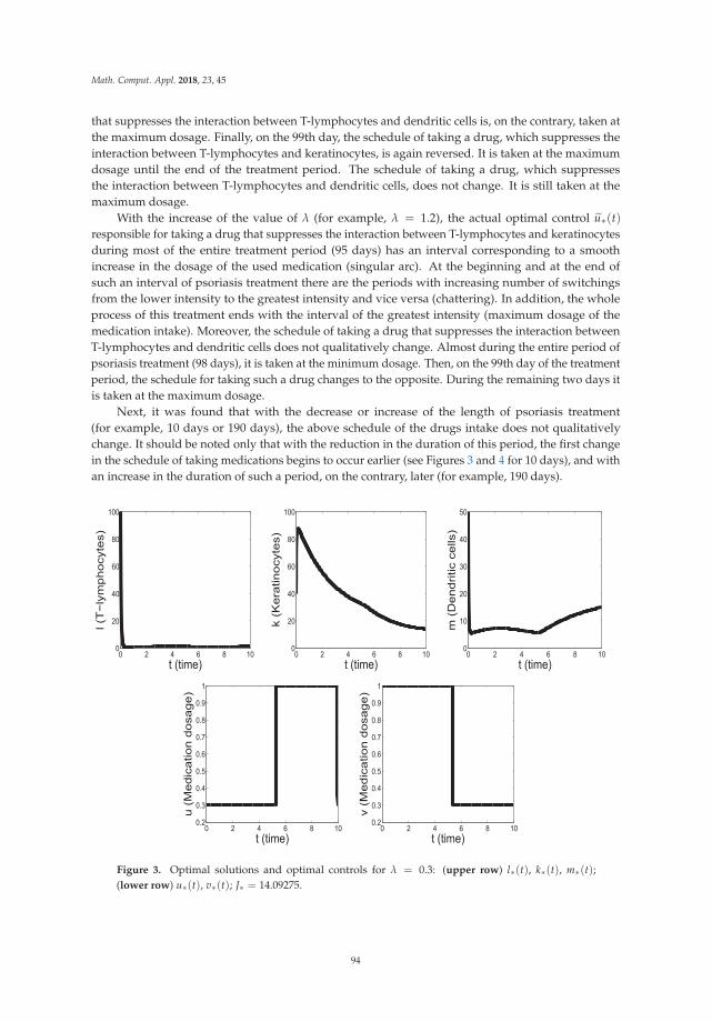
Math. Comput. Appl. 2018, 23, 45
that suppresses the interaction between T-lymphocytes and dendritic cells is, on the contrary, taken atthe maximum dosage. Finally, on the 99th day, the schedule of taking a drug, which suppresses theinteraction between T-lymphocytes and keratinocytes, is again reversed. It is taken at the maximumdosage until the end of the treatment period. The schedule of taking a drug, which suppressesthe interaction between T-lymphocytes and dendritic cells, does not change. It is still taken at themaximum dosage.
With the increase of the value of λ (for example, λ = 1.2), the actual optimal control u∗(t)responsible for taking a drug that suppresses the interaction between T-lymphocytes and keratinocytesduring most of the entire treatment period (95 days) has an interval corresponding to a smoothincrease in the dosage of the used medication (singular arc). At the beginning and at the end ofsuch an interval of psoriasis treatment there are the periods with increasing number of switchingsfrom the lower intensity to the greatest intensity and vice versa (chattering). In addition, the wholeprocess of this treatment ends with the interval of the greatest intensity (maximum dosage of themedication intake). Moreover, the schedule of taking a drug that suppresses the interaction betweenT-lymphocytes and dendritic cells does not qualitatively change. Almost during the entire period ofpsoriasis treatment (98 days), it is taken at the minimum dosage. Then, on the 99th day of the treatmentperiod, the schedule for taking such a drug changes to the opposite. During the remaining two days itis taken at the maximum dosage.
Next, it was found that with the decrease or increase of the length of psoriasis treatment(for example, 10 days or 190 days), the above schedule of the drugs intake does not qualitativelychange. It should be noted only that with the reduction in the duration of this period, the first changein the schedule of taking medications begins to occur earlier (see Figures 3 and 4 for 10 days), and withan increase in the duration of such a period, on the contrary, later (for example, 190 days).
Figure 3. Optimal solutions and optimal controls for λ = 0.3: (upper row) l∗(t), k∗(t), m∗(t);(lower row) u∗(t), v∗(t); J∗ = 14.09275.
94

Math. Comput. Appl. 2018, 23, 45
Figure 4. Optimal solutions and optimal controls for λ = 1.2: (upper row) l∗(t), k∗(t), m∗(t);(lower row) u∗(t), v∗(t); J∗ = 2.644754.
From the comparison of the schedule of the medication intake for 100 days psoriasis treatment,one can conclude that a drug that suppresses the interaction between T-lymphocytes and keratinocytespredominates over a drug that suppresses the interaction between T-lymphocytes and dendritic cells.To show that this predominance is not absolute in psoriasis treatment, we (along with the values of theparameters of System (1), the initial values (2) and the control constraints (3) presented in (104), usethe following values taken from [13]:
σ = 9.0 ρ = 14.0 β = 0.065 δ = 0.01λ = 0.4 μ = 0.07 ν = 0.02 T = 100.0γ1 = 0.0032 γ2 = 0.0002 umin = 0.3 vmin = 0.3l0 = 100.0 k0 = 40.0 m0 = 50.0
The corresponding results of the numerical calculations are given in Figure 5, which include thegraphs of the optimal controls u∗(t), v∗(t), the corresponding optimal solutions l∗(t), k∗(t), and m∗(t),and the minimum value of the functional J(u, v) of (5). From the analysis of the graphs of controlsu∗(t), v∗(t) and Formula (105), we conclude that for the majority of 100 days psoriasis treatment weuse the maximum dosage of a drug suppressing the interaction between T-lymphocytes and dendriticcells. A drug that suppresses the interaction between T-lymphocytes and keratinocytes, should be usedat the minimum dosage for 99 days and only on the last day the schedule of taking this medicationshould be changed to the maximum dosage. This is the first conclusion we draw from Figure 5.The second conclusion is that unlike the results shown in Figures 1 and 3, the first change in theschedule of taking drugs does not occur simultaneously in both, but only in one, which suppresses theinteraction between T-lymphocytes and dendritic cells.
95

Math. Comput. Appl. 2018, 23, 45
Figure 5. Optimal solutions and optimal controls for T = 100.0: (upper row) l∗(t), k∗(t), m∗(t);(lower row) u∗(t), v∗(t); J∗ = 33.185501.
Figure 6 shows that with increasing duration of the period of psoriasis treatment (for example,to 150 days), the actual optimal control v∗(t) responsible for taking a drug that suppresses theinteraction between T-lymphocytes and dendritic cells has a period with a smooth increase in thedosage of the used medication (singular arc).
Figure 6. Optimal solutions and optimal controls for T = 150.0: (upper row) l∗(t), k∗(t), m∗(t);(lower row) u∗(t), v∗(t); J∗ = 33.185511.
96

Math. Comput. Appl. 2018, 23, 45
Finally, the graphs of the optimal solution k∗(t) from Figures 1–6 show that the optimalconcentration of keratinocytes k∗(t) reaches at the end T of the interval [0, T] the level, which isthe minimal for the entire period [0, T] of psoriasis treatment. This fact is very important for thetreatment of the disease.
8. Conclusions
On a given time interval, a nonlinear system of three differential equations describing psoriasistreatment was considered. It established the relationships between the concentrations of T-lymphocytes,keratinocytes, and dendritic cells, which were its phase variables. Also, two scalar bounded controlswere introduced into the system that reflected the doses of drugs aimed at suppressing interactionsbetween T-lymphocytes and keratinocytes, as well as between T-lymphocytes and dendritic cells.The problem of minimizing the concentration of keratinocytes at the final moment of the time intervalwas stated for such a system. To analyze the optimal solution of the minimization problem consistingof the optimal controls and the corresponding optimal solutions of the original system, the Pontryaginmaximum principle was applied. It allowed to obtain the Cauchy problem for the switching functionsdescribing the behavior of the optimal controls. An analysis of this Cauchy problem showed thatsuch controls could be either bang-bang functions, or, in addition to bang-bang intervals, they couldcontain singular arcs. Next, the possibility of simultaneous existence of singular arcs of the optimalcontrols was studied. The orders of singular arcs of such controls were found, the correspondingnecessary optimality conditions for them were checked. Also, the forms of concatenations of singulararcs with nonsingular intervals (where the optimal controls are bang-bang functions) were investigated.After that, the finding of specific optimal solution to the considered minimization problem was carriedout numerically using “BOCOP–2.0.5”. The corresponding results of calculations and their discussionwere provided.
Author Contributions: All authors contributed equally to this work. All authors read and approve the final manuscript.
Acknowledgments: Evgenii Khailov was funded by Russian Foundation for Basic Research according to theresearch project 18-51-45003 IND_a.
Conflicts of Interest: The authors declare no conflict of interest.
References
1. Parisi, R.; Symmons, D.P.; Griffiths, C.E.; Ashcroft, D.M. Global epidemiology of psoriasis: A systematicreview of incidence and prevalence. J. Investig. Dermatol. 2013, 133, 377–385. [CrossRef] [PubMed]
2. Garshick, M.K.; Kimball, A.B. Psoriasis and the life cycle of persistent life effects. Dermatol. Clin. 2015, 33,25–39. [CrossRef] [PubMed]
3. Ryan, C.; Kirby, B. Psoriasis is a systemic disease with multiple cardiovascular and metabolic comorbidities.Dermatol. Clin. 2015, 33, 41–55. [CrossRef] [PubMed]
4. Eder, L.; Chandran, V.; Gladman, D.D. What have we learned about genetic susceptibility in psoriasis andpsoriatic arthritis? Curr. Opin. Rheumatol. 2015, 27, 91–98. [CrossRef] [PubMed]
5. Menter, M.A.; Griffiths, C.E. Psoriasis: The future. Drematol. Clin. 2015, 33, 161–166. [CrossRef] [PubMed]6. Oza, H.B.; Pandey, R.; Roper, D.; Al-Nuaimi, Y.; Spurgeon, S.K.; Goodfellow, M. Modelling and finite-time
stability analysis of psoriasis pathogenesis. Int. J. Control 2017, 90, 1664–1677. [CrossRef]7. Savill, N.J. Mathematical models of hierarchically structured cell populations under equilibrium with
application to the epidermis. Cell Prolif. 2003, 36, 1–26. [CrossRef] [PubMed]8. Niels, G.; Karsten, N. Simulating psoriasis by altering transit amplifying cells. Bioinformatics 2007, 23,
1309–1312.9. Laptev, M.V.; Nikulin, N.K. Numerical modeling of mutial synchronization of auto-oscillations of epidermal
proliferative activity in lesions of psoriasis skin. Biophysics 2009, 54, 519–524. [CrossRef]
97

Math. Comput. Appl. 2018, 23, 45
10. Valeyev, N.V.; Hundhausen, C.; Umezawa, Y.; Kotov, N.V.; Williams, G.; Clop, A.; Ainali, C.; Ouzounis, G.;Tsoka, S.; Nestle, F.O. A systems model for immune cell interactions unravels the mechanism of inflammationin human skin. PLoS Comput. Biol. 2010, 6, e1001024. [CrossRef] [PubMed]
11. Gandolfi, A.; Iannelli, M.; Marinoschi, G. An agestructured model of epidermis growth. J. Math. Biol. 2011,62, 111–141. [CrossRef] [PubMed]
12. Chattopadhyay, B.; Hui, N. Immunopathogenesis in psoriasis throuth a density-type mathematical model.WSEAS Trans. Math. 2012, 11, 440–450.
13. Roy, P.K.; Datta, A. Negative feedback control may regulate cytokines effect during growth of keratinocytesin the chronic plaque of psoriasis: A mathematical study. Int. J. Appl. Math. 2012, 25, 233–254.
14. Zhang, H.; Hou, W.; Henrot, L.; Schnebert, S.; Dumas, M.; Heusèle, C.; Yang, J. Modelling epidermishomoeostasis and psoriasis pathogenesis. J. R. Soc. Interface 2015, 12, 1–22. [CrossRef] [PubMed]
15. Cao, X.; Datta, A.; Al Basir, F.; Roy, P.K. Fractional-order model of the disease psoriasis: A control basedmathematical approach. J. Syst. Sci. Complex. 2016, 29, 1565–1584. [CrossRef]
16. Datta, A.; Roy, P.K. T-cell proliferation on immunopathogenic mechanism of psoriasis: A control basedtheoretical approach. Control Cybern. 2013, 42, 365–386.
17. Roy, P.K.; Datta, A. Impact of cytokine release in psoriasis: a control based mathematical approach.J. Nonlinear Evol. Equ. Appl. 2013, 2013, 23–42.
18. Ledzewicz, U.; Schättler, H. On optimal singular controls for a general SIR-model with vaccination andtreatment. Discret. Contin. Dyn. Syst. 2011, 2, 981–990.
19. Joshi, H.R.; Lenhart, S.; Hota, S.; Agusto, F. Optimal control of an SIR model with changing behavior throughan educational campaign. Electr. J. Differ. Equ. 2015, 2015, 1–14.
20. De Pinho, M.R.; Kornienko, I.; Maurer, H. Optimal control of a SEIR model with mixed constraints andL1 cost. In Controllo’2014—Proceedings of the 11th Portuguese Conference on Automatic Control; Lecture Notes inElectrical Engineering; Springer: Cham, Switzerland, 2015; Volume 321, pp. 135–145.
21. Schättler, H.; Ledzewicz, U. Optimal Control for Mathematical Models of Cancer Therapies. An Application ofGeometric Methods; Springer: New York, NY, USA; Heidelberg, Germany; Dordrecht, The Netherlands;London, UK, 2015.
22. Schättler, H.; Ledzewicz, U. Geometric Optimal Control: Theory, Methods and Examples; Springer: New York,NY, USA; Heidelberg, Germany; Dordrecht, The Netherlands; London, UK, 2012.
23. Roy, P.K.; Bhadra, J.; Chattopadhyay, B. Mathematical modeling on immunopathogenesis in chronic plaqueof psoriasis: A theoretical study. In Proceedings of the World Congress on Engineering, London, UK,30 June–2 July 2010; Volume 1, pp. 550–555.
24. Datta, A.; Kesh, D.K.; Roy, P.K. Effect of CD4+ T-cells and CD8+ T-cells on psoriasis: A mathematical study.Imhotep Math. Proc. 2016, 3, 1–11.
25. Grigorieva, E.; Khailov, E.; Deignan, P. Optimal treatment strategies for control model of psoriasis.In Proceedings of the SIAM Conference on Control and its Applications (CT17), Pittsburgh, PA, USA,10–12 July 2017; pp. 86–93.
26. Datta, A.; Li, X.-Z.; Roy, P.K. Drug therapy between T-cells and DCs reduces the excess production ofkeratinicytes: ausal effect of psoriasis. Math. Sci. Int. Res. J. 2014, 3, 452–456.
27. Lee, E.B.; Marcus, L. Foundations of Optimal Control Theory; John Wiley & Sons: New York, NY, USA, 1967.28. Pontryagin, L.S.; Boltyanskii, V.G.; Gamkrelidze, R.V.; Mishchenko, E.F. Mathematical Theory of Optimal
Processes; John Wiley & Sons: New York, NY, USA, 1962.29. Zelikin, M.I.; Borisov, V.F. Theory of Chattering Control: with Applications to Astronautics, Robotics, Economics
and Engineering; Birkhäuser: Boston, MA, USA, 1994.30. Zorich, V.A. Mathematical Analysis I; Springer: Berlin/Heidelberg, Germany, 2004.31. Bonnans, F.; Martinon, P.; Giorgi, D.; Grélard, V.; Maindrault, S.; Tissot, O.; Liu, J. BOCOP 2.0.5—User Guide.
8 February 2017. Available online: http://bocop.org (accessed on 3 September 018).32. Zelikin, M.I.; Zelikina, L.F. The deviation of a functional from its optimal value under chattering decreases
exponentially as the number of switchings grows. Differ. Equ. 1999, 35, 1489–1493.
98

Math. Comput. Appl. 2018, 23, 45
33. Zelikin. M.I.; Zelikina, L.F. The asymptotics of the deviation of a functional from its optimal value whenchattering is replaced by a suboptimal regime. Russ. Math. Surv. 1999, 54, 662–664. [CrossRef]
34. Zhu, J.; Trélat, E.; Cerf, M. Planar titling maneuver of a spacecraft: Singular arcs in the minimum timeproblem and chattering. Discrete Contin. Dyn. Syst. B 2016, 21, 1347–1388. [CrossRef]
c© 2018 by the authors. Licensee MDPI, Basel, Switzerland. This article is an open accessarticle distributed under the terms and conditions of the Creative Commons Attribution(CC BY) license (http://creativecommons.org/licenses/by/4.0/).
99

Mathematical
and Computational
Applications
Article
Optimal Control Analysis of a Mathematical Modelfor Breast Cancer
Segun Isaac Oke * ID , Maba Boniface Matadi and Sibusiso Southwell Xulu
Department of Mathematical Sciences, University of Zululand, Private Bag X1001, KwaDlangezwa 3886,South Africa; [email protected] (M.B.M.); [email protected] (S.S.X.)* Correspondence: [email protected]
Received: 26 March 2018; Accepted: 20 April 2018; Published: 24 April 2018
Abstract: In this paper, a mathematical model of breast cancer governed by a system of ordinarydifferential equations in the presence of chemotherapy treatment and ketogenic diet is discussed.Several comprehensive mathematical analyses were carried out using a variety of analyticalmethods to study the stability of the breast cancer model. Also, sufficient conditions on parametervalues to ensure cancer persistence in the absence of anti-cancer drugs, ketogenic diet, and canceremission when anti-cancer drugs, immune-booster, and ketogenic diet are included were established.Furthermore, optimal control theory is applied to discover the optimal drug adjustment as an inputcontrol of the system therapies in order to minimize the number of cancerous cells by consideringdifferent controlled combinations of administering the chemotherapy agent and ketogenic diet usingthe popular Pontryagin’s maximum principle. Numerical simulations are presented to validate ourtheoretical results.
Keywords: breast cancer; optimal control; ketogenic diet; chemotherapy
1. Introduction
Cancer is a generic name that refers to a group of diseases in which normal cells divideuncontrollably, that is, grow more rapidly than normal cells, and may eventually spread to other partsof the body by a process called metastasis [1]. According to the National Cancer Registry [2], cancerkills more people than tuberculosis (TB), AIDs and malaria combined. Statistics show that cancerrelated deaths amounted to about 8.2 million in 2010. The mortality rate from cancer is projected tocontinue to rise, with an estimated 13 million deaths by 2030 [3]. The most common types of cancerinclude: breast cancer, prostate cancer, brain cancer, lung cancer and skin cancer among others.
According to the [3] report, breast cancer is the most common invasive cancer in femalesworldwide. The formation of breast cancer can occur in the inner lining of the milk ducts, knownas ductal carcinoma, or in the lobules of the breast, known as lobular carcinoma [4]. Breast cancer isone of the most widely recognized obstructive diseases in females around the world. The disease haspresently been named as the most dangerous cancer in women [3]. However, little is known on thecauses of the ailment. There are three major breast cancer risk factors namely hormonal imbalance(estrogen), genetic (family history), and environmental (poor diet, alcohol consumption, smoking,exposure to toxin, etc.) [5]. Surgery, chemotherapy, radiation therapy, hormonal therapy, hyperthermia,targeted therapy and ketogenic diet [5,6] amongst other therapeutics are used to inhibit tumor growthor kill the tumor cells in the body. However, each treatment has side effects attributed to it, for example,hair loss, vomiting, nausea and fatigue. Adverse effects occur as a result of chemotherapy, which is notable to differentiate between normal cells and tumor cells, consequently killing both of them [3].
Several dietary components and supplements have been examined as possible cancer preventionagents. Until recently, a few studies, such as [6–8], investigated diet as a possible adjuvant to cancer
Math. Comput. Appl. 2018, 23, 21; doi:10.3390/mca23020021 www.mdpi.com/journal/mca100
Math. Comput. Appl. 2018, 23, 21
treatment, which includes a ketogenic diet. A ketogenic diet consists of high edible fat with moderateor low protein content and very low carbohydrates, which forces the body to burn fat instead ofglucose for adenosine triphosphate (ATP) synthesis [6,9].
It is well-known that a mathematical model is a capable device used to investigate the spread ofnon-infectious diseases and to provide important insights into disease behaviors and control [10,11].Over the years, it has become an important tool in comprehending the dynamics of diseases and indecision making processes regarding a medical intervention program for controlling breast cancerin many nations [12]. For instance, [13] explored the role of mathematical modeling on the optimaldelivery of a combination therapy for tumors and to improve on the delivery of anti-tumor drugs.
Old and recent studies such as [4,12,14–16] amongst others have shown that mathematicalmodeling is a widely used tool for resolving questions on public health. For instance, it was usedduring the time of Bernoulli (on modeling the dynamics of Smallpox) in 1760 [17]. Kermack andMcKendrick [14,15] and some other recent studies by [4,12,13,18–21] show that mathematical modelingis useful in solving the problem of epidemiology. However, these studies reveal that much has notbeen done in terms of the mathematical modeling of a nutritional diet (ketogenic diet) as a control ortherapy on tumor cells. Hence, we improved the model in [19] for this paper by incorporating timedependent control parameters (use of ketogenic diet, immune booster, and anti-cancer drugs) basedon the assumption that there is an interaction between normal cells and tumor cells that is due to amutation in DNA as a result of excess estrogen in the body system [4,19,22].
Furthermore, we analyzed and applied an optimal control to the improved model to determine thepossible impacts of ketogenic-diet use and anti-cancer drugs as a treatment on tumor cells. We carriedout a rigorous qualitative optimal control analysis of the resulting model and found the necessaryconditions for optimal control of the disease using Pontryagin’s maximum principle [11,23–25] in orderto determine the optimal strategies for controlling the metastatic of the tumor cells.
This paper is organized as follows: In Section 2, four compartment models of ODEs to study thedynamics of breast cancer are developed. In Section 3, the existence of equilibria, their stabilities andbasic reproductive numbers are discussed. In Section 4, an uncertainty and sensitivity analysis to checkthe most sensitive parameters in the model are discussed. In Section 5, an optimal control problemaccording to the model is proposed and an optimal solution is proffered. Numerical simulations areillustrated by implementing the forward and backward finite difference scheme in Section 6, whileconcluding remarks are provided in Section 7.
2. Model Formulation
Based on the existing model in [19], we developed a model by assuming the logistic (Verhulst)growth of a cell population and basic competition between normal cells and tumor cells. We consideredthe immune cells compartment to comprise Natural Killer cells (NK) and CD8+ T-cells as in [19] andwe used a similar equation to model the immune response dynamic by introducing immune booster(ketone bodies) and anti-cancer drug efficacy.
We adapted an estrogen equation as presented in a model by [26]. Pinho and his co-workersin [26] considered that when a chemotherapy agent is continuously infused into the body and engulfedby different cell populations, natural death can occur. Excess estrogen was used in a similar way andassumed to be saturated daily through birth control (constant source rate) (1 − k). This was introducedto serve as anti-cancer drug efficacy (e.g., Tamoxifen) in order to bind estrogen receptors positive andto reduce excess estrogen from promoting cancer growth [27].
In this study, a model that splits the entire population of cells of the human breast tissues at anygiven period of time P(t) was reflected upon. Hence, normal cells compartment, represented by N(t)in the form of epithelial cells that constitute the breast tissue is described. The cells are assumed todevelop and die normally as they have unaltered DNA that control all cell activities. It was suggested
101

Math. Comput. Appl. 2018, 23, 21
that the normal cells and tumor cells compete for nutrients and other resources in a small volume,which is the competition model used by [28]. Normal cells are represented by
dNdt
= Nα1 − μ1N2 − φ1NT − (1 − k)λ1NE. (1)
The first term represents the logistic growth rate α1 of the normal cells, which are breast tissues thatare made-up of epithelial cells. The second term represents the natural death rate of normal cells. φ1
represents the rate at which normal cells inhibit due to an alteration in DNA that is responsible forcancer cells having an uncontrolled cycle that normal cells do not have [19]. The final term describes thegene transactivation that can be a contributing growth factor responsible for the estrogen stimulationof breast cancer, which can result in damage of DNA. Thus, there will be a reduction in the populationof normal cells N(t) = being transformed into tumor cells by λ1NE where λ1 represents the tumorformation rate resulting from DNA mutation caused by the presence of excess estrogen [4]. However,(1 − k) represents the effectiveness of anti-cancer drugs (Tamoxifen).
The tumor cells compartment can be denoted by T(t) in the form of an abnormal mass of tissue.Tumors are classic signs of inflammation, and can be benign or malignant (cancerous). Their namesusually reflect the kind of tissue from where they arise, for example in breast or brain cancer, amongothers. There are about 51 breast cancer cell lines that mirror the 145 primary breast tumors [29].These can be classified into two major branches: the Luminal, which has estrogen receptors(ESR1 + ve), and the Basal-like, which has no estrogen receptors (ESR1 − ve). A homogeneousluminal type of cancer cells in the form of MDAMB361, MCF-7, BT474, T47D and ZR75 of the celllines [19] are then assumed to be
dTdt
= Tα2d − μ2T2 − γ2MT − μ5T + (1 − k)λ1NE. (2)
The first term of the equation is a limited growth term for tumor cells that depends on the rate ofparameter d (ketogenic diets). Although, if d = 0, tumor cells are automatically eradicated, butany DNA mutation that is caused by excess estrogen will repopulate the tumor cells again λ1NE.The induced death rate μ5 is as a result of tumor starvation of nutrients, glucose and so on from thebody system during the ketogenic diet, which alters nutrition. We assumed that γ2 is the rate at whichtumor cells are being removed due to the effectiveness of immune response.
The immune response compartment is represented by M(t) in the form of natural killer (NK)cells and CD8+ T cells. Their growth may be stimulated by the presence of the tumor and they candestroy tumor cells through the kinetics process. We also assumed that the presence of a detectabletumor in a body system does not necessarily imply that the tumor has completely escaped activeimmunosurveillance. However, a tumor is immunogenic. It is possible that the immune response maynot be sufficient on its own to completely combat the rapid growth of the tumor cells population andtheir eventual development into a tumor.
dMdt
= sβ +ρMTω + T
− γ3MT − μ3M −((1 − k)
λ3MEg + E
)(3)
The constant source parameter s denotes the source rate of immune response fully infused in thebody daily. We introduced immune booster β (a supplement such as ketone bodies) to assist immuneresponse whenever tumor cells overpower immune cells in order to activate the immune response andfight the cancer cells. The next term is a nonlinear growth term for immune response where ρ the rateof immune response is and ω is the immune cell threshold [12]. We denoted γ3 as the rate at whichimmune response is inactivated upon interacting with tumor cells while μ3 represents the immunecells natural death rate as a result of necrosis. The final term explains a limited rate at which estrogensuppresses immune cells activation where λ3 is the rate of immune suppression and g is the estrogenthreshold [19].
102

Math. Comput. Appl. 2018, 23, 21
Finally, we considered estrogen compartment denoted by E(t). Estrogen is a female steroidhormone that is produced by the ovaries in lesser amounts, and by the adrenal cortex, placenta andmale testes. Estrogen helps to control and guide sexual development, including the physical changesassociated with puberty [11,30]. However, an increase in estrogen levels can lead to the growth of thetumor cells. It also serves as a mitogen by triggering cell division in breast tissue [30]. Estrogen acts asa carcinogen by directly damaging DNA, forcing healthy epithelial cells to have a higher likelihood ofmalignant conversion [5,30].
dEdt
= (1 − k)ε − μ4E (4)
The process of constantly replenishing excess estrogen is denoted by ε. We assumed that themajority of cancer cells are estrogen-receptor positive and only a small proportion of epithelial cellsare estrogen-receptor positive, which can only be blocked by the anti-cancer drug (1 − k) Tamoxifen.μ4 is the rate at which estrogen is being washed out from the body system. Thus, system (5) is ourmodified model.
dNdt = N(α1 − μ1N − φ1T)− (1 − k)(λ1NE)
dTdt = T(α2d − μ2T)− γ2MT − μ5T + (1 − k)(λ1NE)dMdt = sβ + ρMT
ω+T − γ3MT − μ3M −((1 − k) λ3 ME
g+E
)dEdt = (1 − k)ε − μ4E
(5)
3. Model Analysis
3.1. Boundedness and Positivity of Solutions
The system of Equation (5) has an initial condition by
N(0) = N0 ≥ 0, T(0) = T0 ≥ 0, M(0) = M0 ≥ 0, and E(0) = E0 ≥ 0
since our model is to investigate cellular populations, therefore all the variables and parameters of themodel are non-negative. Based on the biological finding, the system of Equation (5) will be studied inthe following region such as:
Δ ={(N, T, M, E) ∈ �4
+
}The following theorem assures that the system of Equation (5) is well-posed such that solutions
with non-negative initial conditions remain non-negative for all 0 < t < ∞, and therefore makes thevariable biologically meaningful. Hence, we have the following result:
Theorem 1. The region Δ ⊂ �4+ is positively invariant with respect to the system of Equation (5) and
non-negative solution exists for all time 0 < t < ∞.
Proof: Let Δ = Δc ⊂ �4+ with Δ = {(N, T, M, E) ∈ �4
+ : N ≤ α1μ1}, then the solutions (N (t), T(t), M(t),
E(t)) of system (5) are positive ∀t ≥ 0. It is obvious from the first compartment of system (5) that
dNdt
≤ N(t)α1 − μ1N2(t).
Solving with Bernoulli method and taking N(0) = N0, we have
N(t) ≤ α1
μ1 + kα1e−α1t
withk =
α1 − N0μ1
N0α1
103

Math. Comput. Appl. 2018, 23, 21
N0 =α1
μ1 + kα1.
Then,N(t) ≤ α1
μ1 +(
α1−N0μ1N0
)e−α1t
N(t) ≤ α1
μ1as t → ∞
hence, N(t) > 0, ∀t > 0 and if and only if (1 − k) ≥ 0 [31].Consequently, it can be shown that T(t) > 0, M(t) > 0, and E(t) > 0 ∀t > 0. This completes
the proof. �
3.2. The Equilibrium Points of System (5)
The steady states occur by setting the left hand side (LHS) of system (5) to zero, i.e.,
dNdt
=dTdt
=dMdt
=dEdt
= 0
The model system admits six steady states in which there are four dead equilibria, one tumor-freeequilibrium point and one co-existing equilibrium point P = (N∗, T∗, M∗, E∗) where N∗, T∗, M∗, E∗
represent the tumor-free equilibrium values for the normal cells, tumor cells, immune cells and estrogenhormone respectively. We have N∗ > 0, M∗ > 0, E∗ > 0 since cell populations are non-negative andreal. Therefore, all parameters s,β, g, μ1, μ3, μ4, ε, λ3, k, α1, and λ1 are positive.
Tumor-Free equilibrium point
P0 =
(α1μ4 − (1 − k)2λ1ε
μ1μ4, 0,
sβ(gμ4 + (1 − k)ε)
μ3(gμ4 + (1 − k)ε) + (1 − k)2λ3ε,(1 − k)ε
μ4
)
Type 1 Dead equilibrium point
Pd1 =
(0, 0,
sβ(gμ4 + (1 − k)ε)
μ3(gμ4 + (1 − k)ε) + (1 − k)2λ3ε),(1 − k)ε
μ4
)
Type 2 Dead equilibrium point
Pd2 =
(0,
dα2 − γ2m∗1 − μ5
μ2, m∗
1,(1 − k)ε
μ4
)Type 3 Dead equilibrium point
Pd3 =
(0,
dα2 − γ2m∗2 − μ5
μ2, m∗
2,(1 − k)ε
μ4
)Type 4 Dead equilibrium point
Pd4 =
(0,
dα2 − γ2m∗3 − μ5
μ2, m∗
3,(1 − k)ε
μ4
)Co-existing equilibrium point
Pe = (N∗4 , T∗
4 , M∗4 , E∗
4 )
104

Math. Comput. Appl. 2018, 23, 21
3.3. The Reproductive Number and Tumor-Free Equilibrium Point
In this section, we mainly analyzed the stability behaviors of system (5) by means of eigenvalues.We apply Hartman–Grobman Theorem which states that in the neighborhood of a hyperbolicequilibrium point, a nonlinear dynamical system is topologically equivalent to its linearization [32].
Theorem 2. The tumor-free equilibrium (TFE) point P0 of system (5) is locally asymptotically stable if R0 < 1,otherwise unstable.
Proof. Linearizing system (5) around TFE P0, we obtained the following Jacobian matrix J(P0)
J =
⎛⎜⎜⎜⎜⎝2μ1λ1(1−k)2ε−α1μ1μ4−(1−k)2λ1μ1ε
μ1μ4
(1−k)2λ1Φ1ε−Φ1α1μ4μ1μ4
0 −B6(1−k)2λ1ε
μ4B3 0 B6
0 B4 −B5 −B7
0 0 0 −μ4
⎞⎟⎟⎟⎟⎠
J(P0) =
⎛⎜⎜⎜⎝B0 B2 0 −B6
B1 B3 0 B6
0 B4 −B5 −B7
0 0 0 −μ4
⎞⎟⎟⎟⎠
|J(P0)| =
∣∣∣∣∣∣∣∣∣∣∣B0 − δ B2 0 −B6
B1 B3 − δ 0 B6
0 B4 −B5 − δ −B7
0 0 0 −μ4 − δ
∣∣∣∣∣∣∣∣∣∣∣= 0
Then the characteristic equation at P0 of the linearized system of the model (5) is given below.Obviously, there exists two negative characteristic roots
δ1 = −μ4, δ2 = −B5
However, we only need to consider
δ2 − (B0 + B3)δ + B0B3 − B1B2 = 0
δ2 − (B0 + B3)δ + B0B3
(1 − B1B2
B0B3
)= 0 (6)
from (6), we have basic reproduction number
R0 =B1B2
B0B3(7)
δ2 − (B0 + B3)δ + B0B3(1 − R0) = 0,
where
B0 =2μ1λ1(1 − k)2ε − α1μ1μ4 − (1 − k)2λ1μ1ε
μ1μ4, B1 =
(1 − k)2λ1ε
μ4, B2 =
(1 − k)2λ1Φ1ε − Φ1α1μ4
μ1μ4
B3 =α2μ3dψ∗ + α2λ3dε(1 − k)2 − γ2sβψ∗ − μ5μ3ψ∗ − μ5λ3ε(1 − k)2
μ3ψ∗ + (1 − k)2λ3ε
105

Math. Comput. Appl. 2018, 23, 21
whereψ∗ = (gμ4 + (1 − k)ε)
− B4 =sβ(gμ4 + (1 − k)ε(ρ − γ3ω)
ωμ3(gμ4 + (1 − k)ε)
− B5 =μ3μ4g + μ3(1 − k)ε + λ3(1 − k)2ε
gμ4 + (1 − k)ε,−B6 = −
((1 − k)λ1α1μ4 − (1 − k)3λ2
1ε
μ1μ4
)
B6 =(1 − k)λ1α1μ4 − (1 − k)3λ2
1ε
μ1μ4,−B7 = −
⎛⎝ μ24(1 − k)λ3gsβ(gμ4 + (1 − k)ε)
(gμ4 + (1 − k)ε)2[μ3(gμ4 + (1 − k)ε) + (1 − k)2λ3ε
]⎞⎠
Here, we can apply the Routh-Hurwitz criterion namely,
(i) Tr(A) < 0 (ii) Det(A) > 0
provideda0 = 1 > 0, a1 = (B0 + B3) < 0, B0B3(1 − R0) > 0 if R0 < 1,
B0B3 > B1B2, B1 > 0, B2 > 0, B3 < 0, B0 < 0
Since the Routh–Hurwitz criterion holds, all the eigenvalues are negative, i.e., δ3 < 0 and δ4 < 0.Therefore, the TFE point of system (5) is locally asymptotically stable if (7) R0 < 1 otherwise unstable.�
The epidemiological implication of the above result is that the tumor cells that are governed bysystem (5) can be eliminated from the population (normal cells or breast tissues) whenever an influxby tumor cells into the normal cells is small, such that R0 < 1. Therefore, the existence of a tumor-freeequilibrium in this case depends on the estrogen level.
Theorem 3. The Type 1 Dead equilibrium point Pd1 of system (5) is locally asymptotically stable if((1 − k)2λ1ε
α1μ4
)> 1,
otherwise unstable.
Proof. Linearizing system (5) around the Type 1 Dead free equilibrium point Pd1, we obtained thefollowing Jacobian matrix J(Pd1)
J =
⎛⎜⎜⎜⎜⎝α1 − (1 − k)λ1E∗
0 0 0 0(1 − k)λ1E∗
0 dα2 − γ2M∗0 − μ5 0 0
0 ρωM∗0−γ3 M∗
0 ω2
ω2 −(
μ3(g+E∗0 )+(1−k)λ3E∗
0(g+E∗
0 )
)λ3gM∗
0 (1−k)(g+E∗
0 )2
0 0 0 −μ4
⎞⎟⎟⎟⎟⎠
J(Pd1) =
⎛⎜⎜⎜⎝C0 0 0 0C1 C2 0 00 C3 −C4 −C5
0 0 0 −μ4
⎞⎟⎟⎟⎠
106

Math. Comput. Appl. 2018, 23, 21
|J(P1)| =
∣∣∣∣∣∣∣∣∣∣∣C0 − δ 0 0 0
C1 C2 − δ 0 00 C3 −C4 − δ −C5
0 0 0 −μ4 − δ
∣∣∣∣∣∣∣∣∣∣∣= 0
Clearly, two eigenvalues of the system (5) at Pd1 are negative and real
δ1 = −μ4
and
δ2 = −C4 ⇒ −(
μ3(gμ4 + (1 − k)ε) + (1 − k)2λ3ε
gμ4 + (1 − k)ε
)while the remaining two eigenvalues are obtained from 2 × 2 matrix.
A =
⎛⎜⎝ C0 0C1 C2
⎞⎟⎠Applying the Routh-Hurwitz criterion stated above; we have
(i) Tr(A) =C0 + C2 ⇒(
α1μ4−(1−k)2λ1εμ4
+ (μ3α2d−γ2sβ−μ5μ3)A∗+dα2λ3(1−k)2ε−(1−k)2λ3μ5ε
μ3 A∗+(1−k)2λ3ε
)< 0
i f α1
(1 − (1−k)2λ1ε
α1μ4
)> 0,⇒
((1−k)2λ1ε
α1μ4
)> 1
Therefore, Tr(A) < 0
(ii) Det(A) =C0C2((α1μ4−(1−k)2λ1ε
μ4
)((μ3α2d−γ2sβ−μ5μ3)A∗+dα2λ3(1−k)2ε−(1−k)2λ3μ5ε
μ3 A∗+(1−k)2λ3ε
))> 0
i f α1
(1 − (1−k)2λ1ε
α1μ4
)> 0 provided
((1−k)2λ1ε
α1μ4
)> 1
and{(α1
(1 − (1 − k)2λ1ε
α1μ4
))(((μ3α2d − γ2sβ − μ5μ3)A∗ + dα2λ3(1 − k)2ε − (1 − k)2λ3μ5ε
μ3 A∗ + (1 − k)2λ3ε
))}> 0
implies that Det(A) > 0. Thus, the remaining eigenvalues δ3 and δ4 are negative and real since R-Hcriterion has been satisfied. Hence, the type 1 Dead equilibrium point Pd1 of the system (5) is locally
asymptotically stable if(
(1−k)2λ1εα1μ4
)> 1. �
Epidemiologically it is implied that the net growth of the tumor cells must be more than theimmune cells values in order to have the tumor cells overpower the normal cells as the reactivation ofthe immune cells is due to the estrogen effects that are greater than the reactivation of the immunecells due to the tumor effect. However, ketogenic diet is inactive at the type 1 Dead equilibrium point.
Theorem 4. The Type 2 Dead equilibrium point Pd2 of system (5) is locally asymptotically stable if((1 − k)2λ1ε
α1μ4
)> 1
107
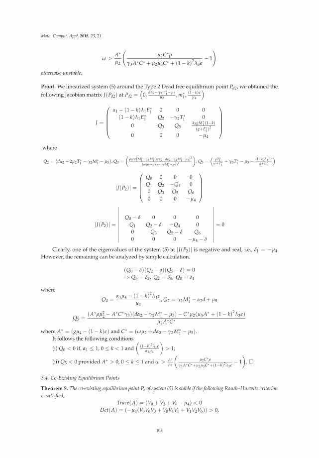
Math. Comput. Appl. 2018, 23, 21
ω >A∗
μ2
(μ2C∗ρ
γ3 A∗C∗ + μ2μ3C∗ + (1 − k)2λ3ε− 1
)otherwise unstable.
Proof. We linearized system (5) around the Type 2 Dead free equilibrium point Pd2, we obtained thefollowing Jacobian matrix J(Pd2) at Pd2 =
(0, dα2−γ2m∗
1−μ5μ2
, m∗1, (1−k)ε
μ4
)
J =
⎛⎜⎜⎜⎜⎝α1 − (1 − k)λ1E∗
1 0 0 0(1 − k)λ1E∗
1 Q2 −γ2T∗1 0
0 Q3 Q5λ3gM∗
1 (1−k)(g+E∗
1 )2
0 0 0 −μ4
⎞⎟⎟⎟⎟⎠where
Q2 =(dα2 − 2μ2T∗
1 − γ2M∗1 − μ5
), Q3 =
(ρωμ2
2 M∗1−γ3 M∗
1 (ωμ2+dα2−γ2 M∗1−μ5)
2
(ωμ2+dα2−γ2 M∗1−μ5)
2
), Q5 =
(ρT∗
1ω+T∗
1− γ3T∗
1 − μ3 − (1−k)λ3E∗1
g+E∗1
)
|J(P2)| =
⎛⎜⎜⎜⎝Q0 0 0 0Q1 Q2 −Q4 00 Q3 Q5 Q6
0 0 0 −μ4
⎞⎟⎟⎟⎠
|J(P2)| =
∣∣∣∣∣∣∣∣∣∣∣Q0 − δ 0 0 0
Q1 Q2 − δ −Q4 00 Q3 Q5 − δ Q6
0 0 0 −μ4 − δ
∣∣∣∣∣∣∣∣∣∣∣= 0
Clearly, one of the eigenvalues of the system (5) at |J(P2)| is negative and real, i.e., δ1 = −μ4.However, the remaining can be analyzed by simple calculation.
(Q0 − δ)(Q2 − δ)(Q5 − δ) = 0⇒ Q5 = δ2, Q2 = δ3, Q0 = δ4
where
Q0 =α1μ4 − (1 − k)2λ1ε
μ4, Q2 = γ2M∗
1 − α2d + μ5
Q5 =(A∗ρμ2
2 − A∗C∗γ3)(dα2 − γ2M∗1 − μ5)− C∗μ2(μ3 A∗ + (1 − k)2λ3ε)
μ2 A∗C∗
where A∗ = (gμ4 − (1 − k)ε) and C∗ = (ωμ2 + dα2 − γ2M∗1 − μ5).
It follows the following conditions
(i) Q0 < 0 if, α1 ≤ 1, 0 ≤ k < 1 and(
(1−k)2λ1εα1μ4
)> 1;
(ii) Q5 < 0 provided A∗ > 0, 0 ≤ k ≤ 1 and ω > A∗μ2
(μ2C∗ρ
γ3 A∗C∗+μ2μ3C∗+(1−k)2λ3ε− 1
). �
3.4. Co-Existing Equilibrium Points
Theorem 5. The co-existing equilibrium point Pe of system (5) is stable if the following Routh–Hurwitz criterionis satisfied,
Trace(A) = (V0 + V3 + V6 − μ4) < 0Det(A) = (−μ4(V0V6V3 + V0V4V5 + V1V2V6)) > 0,
108

Math. Comput. Appl. 2018, 23, 21
otherwise unstable.
Proof. We analyzed and linearized system (5) around the co-existing equilibrium point Pe, weobtained the following Jacobian matrix J(Pe) at Pe = (N∗
4 , T∗4 , M∗
4 , E∗4 ) where N∗
4 , T∗4 , M∗
4 & E∗4
represent the coexisting equilibrium values for normal cells, tumor cells, immune cells, and estrogenlevels respectively.
A co-existing equilibrium state exists when all cells populations would have survivedthe competition.
N∗4 =
2(1 − k)4λ41μ1μ4ε2 + φ1α2
1μ24μ1 − 2(1 − k)2μ1μ2
4α1λ1φ1ε − 2α1φ21μ1μ3
4 − 2(1 − k)2α1μ1μ24λ1ε
2φ1α1μ21μ3
4 − 2(1 − k)2μ21μ2
4λ1φ1ε
T∗4 =
α21μ1μ2
4 + 2α1μ1μ24φ1
2φ1α1μ1μ24 − 2(1 − k)2μ1μ4λ1φ1ε
M∗4 =
G∗2Z∗(1−k)2λ1ε+(α2
1α2μ1μ34d+2α1α2μ1μ3
4φ1d−μ34μ5α2
1−2μ34μ1μ5α1φ1)G∗−μ3α4
1μ21μ5
4−4α21μ2
1μ2μ54φ1−4φ2
1α21μ2
1μ54μ2
G∗2 Q∗μ4
E∗4 =
(1 − k)εμ4
whereG∗2
= 2φ1α1μ1μ24 − 2(1 − k)2μ1μ4λ1φ1ε
Z∗ =2(1 − k)4λ2
1μ1μ4ε2 + φ1α21μ2
4μ1 − 2(1 − k)2μ1μ24α1λ1φ1ε − 2α1φ2
1μ1μ34 − 2(1 − k)2α1μ1μ2
4λ1ε
2φ1α1μ21μ3
4 − 2(1 − k)2μ21μ2
4λ1φ1ε
Q∗ =α2
1μ1μ24γ2 − 2α1μ1μ2
4φ1γ2
2φ1α1μ1μ24 − 2(1 − k)2μ1μ4λ1φ1ε
J =
⎛⎜⎜⎜⎜⎝(α1 − 2μ1N∗
4 − (1 − k)λ1E∗4) −N∗
4 φ 0 −V7
(1 − k)λ1E∗4
(dα2 − 2μ2T∗
4 − γ2M∗4 − μ5
) −γ2T∗4 V7
0 V4 V6λ3gM∗
4 (1−k)(g+E∗
4 )2
0 0 0 −μ4
⎞⎟⎟⎟⎟⎠
A =
⎛⎜⎜⎜⎝V0 −V2 0 −V7
V1 V3 −V5 V7
0 V4 V6 V8
0 0 0 −μ4
⎞⎟⎟⎟⎠
|A| =
∣∣∣∣∣∣∣∣∣∣∣V0 −V2 0 −V7
V1 V3 −V5 V7
0 V4 V6 V8
0 0 0 −μ4
∣∣∣∣∣∣∣∣∣∣∣= 0
We need to show that Trace(A) < 0, that is
Tr(A) = (V0 + V3 + V6 − μ4) < 0
= α1(1 − A0)− 2μ1N∗4 + dα2(1 − μ5)− μ4 +
T∗4(ρ − γ3(ω − T∗
4 ))
ω + T∗4
− μ3 − (1 − k)4λ3ε
(gμ4 + (1 − k)ε
Thus,
Tr(A) < 0, if A0 > 1, μ5 > 1, ρ < γ3(ω + T∗4 ) with A0 =
(1 − k)2λ3ε
α1μ4
109

Math. Comput. Appl. 2018, 23, 21
To show that,|A|= (−μ4(V0V3V6 + V0V4V5 + V1V2V6)) > 0
Let ζ1 = −μ4V0V3V6, ζ2 = −μ4V0V4V5, ζ3 = −μ4V1V2V6
ζ1 =(α1(1 − A0)− 2μ1N∗
4)(
dα2(1 − μ5)− 2μ2T∗4 − γ2μ∗
4))( T∗
4 (ρ−γ3(ω−T∗4 ))
ω+T∗4
− μ3 − (1−k)4λ3ε(gμ4+(1−k)ε
).
This implies that, ζ1 > 0 is a positive, if A0 > 1, μ5 > 1, ρ < γ3(ω + T∗4 ) with A0 = (1−k)2λ3ε
α1μ4
ζ2 = (α1(1 − A0)− 2μ1N∗4 )
(M∗
4
(ω + T∗4 )
2 (ρω − γ3(ω + T∗4 ))
)(−γ2T∗
4 )
This implies that, ζ2 > 0 is a positive, if A0 > 1, μ5 > 1, ρω < γ3(ω + T∗4 )
2, with A0 = (1−k)2λ3εα1μ4
ζ3 = −μ4(A0)(−φ1N∗4 )
(T∗
4(ρ − γ3(ω − T∗
4 ))
ω + T∗4
− μ3 − (1 − k)4λ3ε
(gμ4 + (1 − k)ε
)
This implies that ζ3 < 0 is a negative and by Routh-Hurwitz criterion the system cannot be stable.Thus the co-existing equilibrium point is always unstable if the cells coexist where
V0 =α1μ4 − 2μ1μ4N∗
4 − (1 − k)2λ1ε
μ4, V1 =
(1 − k)2λ1ε
μ4, V2 = −φ1N∗
4 ,
V3 = (dα2 − 2μ2T∗4 − γ2M∗
4 − μ5), V4 =ρM∗
4 ω − γ3M∗4(ω + T∗
4 )2
(ω + T∗4 )
2 , V5 = −γ2T∗4
V6 =ρT∗
4 (gμ4+(1−k)ε)−γ3T∗4 (ω+T∗
4 )(gμ4+(1−k)ε)−μ3(ω+T∗4 )(gμ4+(1−k)ε)−(1−k)2(ω+T∗
4 )λ3ε
(ω+T∗4 )(gμ4+(1−k)ε)
− V7 = −(1 − k)λ1N∗4 , V7 = (1 − k)λ1N∗
4 , V8 =λ3μ2
4gM∗4(1 − k)
(gμ4 + (1 − k)ε)2
�
4. Uncertainty and Sensitivity Analysis
In this section, we explore the dependence of the model solutions on the parameter values. We areable to figure-out a feasible range of parameter values and determine the most critical parametersin the model. We employed a similar method, which is discussed in detail by [20,33], using LatinHypercube Sampling (LHS) for studying the uncertainty analysis and the Partial Rank CorrelationCoefficient (PRCC) for analyzing the sensitivity analysis indexes of the parameters. LHS/PRCC wasran and analyzed with a sample size of 100. The choice of this sample size is due to the fact that PRCCproduces accurate results for a lower sample size compared to other technique, such as eFAST [33].
Uncertainty and sensitivity analysis were performed on all non-dimensional system parameters inthe system (5) with the aim of determining the most sensitive parameters to the model. The parameterbaseline values in Table 1 were varied in the range of 25%. Figure 1 displays a bar graph of PRCCsplotted against the homogeneous parameter value with tumor compartment as the baseline dependentvariable. The parameters that are significantly positively correlated with tumor cells, at P < 0.05level of significance, are α1, g while μ1, γ3, and ω are significantly negatively correlated. An increasein the production of normal cells α1, leads to higher numbers of normal cells, thus the higher theα1, the higher the normal cells. While Figure 2 displays a bar graph of PRCCs plotted against thehomogeneous parameter value with tumor compartment as the baseline dependent variable. The mostsensitive parameters are shown to be P − values of s, γ2, μ3 and ρ are less than 0.01.
110
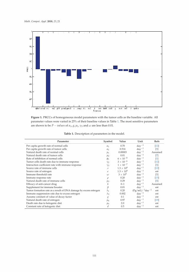
Math. Comput. Appl. 2018, 23, 21
Figure 1. PRCCs of homogeneous model parameters with the tumor cells as the baseline variable. Allparameter values were varied in 25% of their baseline values in Table 1. The most sensitive parametersare shown to be P − values of α1, g, μ1, γ3 and ω are less than 0.01.
Table 1. Description of parameters in the model.
Parameter Symbol Value Unit Refs
Per capita growth rate of normal cells α1 0.70 day−1 [12]Per capita growth rate of tumor cells α2 0.514 day−1 [5]Natural death rate of normal cells μ1 0.00003 day−1 AssumedNatural death rate of tumor cells μ2 0.01 day−1 [7]Rate of inhibition of normal cells φ1 6 × 10⁻⁸ day−1 [1]Tumor cells death rate due to immune response γ2 3 × 10⁻⁶ day−1 [12]Interaction coefficient rate with immune response γ3 1 × 10⁻⁷ day−1 [5]Source rate of immune cells s 1.3 × 10⁴ day−1 [12]Source rate of estrogen ε 1.3 × 10⁴ day−1 estImmune threshold rate ω 3 × 10⁵ day−1 [5]Immune response rate ρ 0.20 day−1 [13]Natural death rate of immune cells μ3 0.29 day−1 [5]Efficacy of anti-cancer drug k 0–1 day−1 AssumedSupplement for immune booster β 0.01 day−1 estTumor formation rate as a result of DNA damage by excess estrogen λ1 0.20 (Pg/mL)−1day−1 estImmune suppression rate due to excess estrogen λ3 0.002 day−1 estAssume constant of value of decay factor g 0.1 day−1 estNatural death rate of estrogen μ4 0.97 day−1 [19]Death rate due to ketogenic diet μ5 2.0 day−1 estConstant rate of ketogenic diet d 0.5 day−1 est
111

Math. Comput. Appl. 2018, 23, 21
Figure 2. PRCCs of homogeneous model parameters with the tumor cells as the baseline variable.All parameter values were varied in 25% of their baseline values in Table 1. The most sensitiveparameters are shown to be P − values of s, γ2, μ3 and ρ are less than 0.01.
5. Analysis of Optimal Control
In this section, we formulated a corresponding optimal control problem for the model in thesystem (5) considering ketogenic-diet and anti-cancer drugs as control interventions to minimize thebreast cancer and tumor burden at final time. The units of cells were normalized in order for thecarrying capacity of normal cells to be kept above threshold of 0 ≤ t ≤ t f [34–36]. On the other hand,the aim is to reduce the tumor-size which indicates the degree of the disease in the body and it requiresthe application of as much anti-cancer drugs as much as possible. However, it also minimized thesystemic cost, which is based on the quantities of anti-cancer drugs, since large drug concentrationscan be harmful and cause toxic side effects. In brief, the drug doses were minimized because thesmaller the dose, the better. Then, we formulated the objective functional J1
J1(u1, u2) =∫ Tf
0
(A1T(t) + A2E(t) +
12
A3u21(t) +
12
A4u22(t)
)dt (8)
System equations (5) is subject to:
dNdt = Nα1 − μ1N2 − φ1TN − (1 − u1(t))(λ1NE)
dTdt = (1 − u2(t))Tα2 − μ2T2 − γ2MT − μ5T + (1 − u1(t))(λ1NE)dMdt = sβ + ρMT
ω+T − γ3MT − μ3M −((1 − u1(t))
λ3 MEg+E
)dEdt = (1 − u1(t))ε − μ4E
(9)
J1 involves a quadratic control. In [37–41], it was established that quadratic control in the treatmentterms has the added benefit of keeping the tumor in check both when it is small or large in size.The authors further explained that the quadratic control allows for a weaker treatment to minimizethe toxic side-effects while permitting the system to maintain a low tumor size.
Furthermore, for us to address the tumor-to-therapy trade-off, we established the existenceof an optimal control; by following the approach in [37,41,42], which required an analysis of the
112

Math. Comput. Appl. 2018, 23, 21
super-solutions (that is, the upper bounds on solutions) of the system (5). As soon as we were able toshow that the system is bounded, we established the existence of an optimal control using a resultfrom [43]. In addition, we proved that there exists an optimal control that minimizes the objectivefunctional; using the established approach of [37–40,44]. We use the fact that super-solutions N, T, M,E of
dNdt = Nα1, dT
dt = Tα2(1 − u2),dMdt = sβ + ρMT
ω+T , dEdt = 1
(10)
are bounded on a finite time interval. Since the sub-solutions are zero, the result obtained shows thatour system is bounded. Since we have a bounded system, our next task was to establish the existenceof the optimal control using a result from [43].
Existence of an Optimal Control
Theorem 6. Given the objective functional in (8), where U ={u∗
i (t), Lebesguemeasure : 0 ≤ u∗i (t) ≤ 1, ∀t ∈ [0, t]
}subject to system (9) with N(0) = N0,
T(0) = T0, M(0) = M0, and E(0) = E0, then there exists an optimal control u∗i such that
minu∗i (t)∈[0,1] J1(u∗
i ) = J1(u∗i (t)) if the following conditions holds:
• f is not empty;• The admissible control set U is closed and convex;• Each right hand side of the state system is continuous, is bounded above by the sum of the
bounded control and the state, and can be written as a linear function of u∗i (t) with coefficients
depending on time and the state;• The integrand of J1(u∗
i ) is convex on U and is bounded below by −c2 + c1u2 with c1 > 0.
Proof. Since the system (9) has bounded coefficients and the solutions are bounded on the finitetime interval, we can apply the result of [45], to obtain the existence of the solution of the system (9).Furthermore, we note that U is closed and convex by definition. For the third conditions, the right handside of the system (9) must be continuous. The right hand side is continuous since the denominators of
all fractions from the right hand side of the system consists solely of positive entities. We let←φ (t,
←X) be
right hand side of the system (9) except for the terms of u∗i and define.
|←f (t,
←X, u∗
i )| =←φ (t,
←X) +
⎛⎜⎜⎜⎜⎜⎝0
λ1NE0u1
⎞⎟⎟⎟⎟⎟⎠, with←X =
⎛⎜⎜⎜⎜⎜⎝NTME
⎞⎟⎟⎟⎟⎟⎠using the boundedness of the solutions (10), we have
|←f (t,
←X, u∗
i )| ≤
∣∣∣∣∣∣∣∣∣∣∣
⎛⎜⎜⎜⎜⎜⎝α1 0 0 00 α2(1 − u2) 0 00 0 ρ 00 0 0 0
⎞⎟⎟⎟⎟⎟⎠
⎛⎜⎜⎜⎜⎜⎝NTME
⎞⎟⎟⎟⎟⎟⎠
∣∣∣∣∣∣∣∣∣∣∣+
∣∣∣∣∣∣∣∣∣∣∣
⎛⎜⎜⎜⎜⎜⎝0
(1 − u1)λ1NEsβ
−u1ε
⎞⎟⎟⎟⎟⎟⎠
∣∣∣∣∣∣∣∣∣∣∣≤ c1
(|←X|+ |
←u∗
i |)
where c1 depends on the coefficients of the system. For the fourth condition, we need to show
J(t, T, E, (1 − Pi)ui + PiVi) ≤ (1 − Pi)J(t, T, E, ui) + Pi(t, T, E, Vi)
113

Math. Comput. Appl. 2018, 23, 21
we analyze the difference of
J(t, T, E, (1 − Pi)ui + PiVi)− [(1 − Pi)J(t, T, E, ui) + Pi(t, T, E, Vi)]
= T(t) + E(t) + ε2(u2
i − 2Piu2i + P2
i u2i + P2
i V2i − 2P2
i V2i u2
i + 2PiViui)
−(T(t) + E(t) + ε2 u2
i − ε2 Piu2
i +ε2 PiV2
i)
=ε
2(P2
i − Pi)(ui − Vi)2
since, Pi ∈ (0, 1) implies (P2i − Pi) < 0 and (ui − Vi)
2 > 0 but (P2i − Pi) < 0, which implies ε
2 (P2i −
Pi)(ui − Vi)2 is negative. This implies that,
J(t, T, E, (1 − Pi)ui + PiVi) ≤ (1 − Pi)J(t, T, E, ui) + Pi(t, T, E, Vi)
Lastly,
T(t) + E(t) +ε
2u2
i (t) ≥ε
2u2
i (t) ≥ −c +ε
2u2
i (t)
which gives −c + ε2 u2
i (t) as the lower bound. With the existence of the optimal control established, wenow characterized the optimal control using the Pontryagin’s maximum principle [11]. The constantsA1, A2, A3 and A4 are a measure of the relative cost of the interventions over [0, T]. The optimal controlproblem is that of finding optimal functions (u∗
1(t), u∗2(t)) such that
J1(u∗1(t), u∗
2(t)) = minΩ
J1(u1(t), u2(t)) (11)
whereΩ =
{u1(t)&u2(t) : 0 ≤ u1(t) ≤ u1max, 0 ≤ u2(t) ≤ u2max, t ∈ [0, Tf ]
}�
Three different control strategies are explored. This approach can be used to test various options.However, we only looked at the following three alternatives:
• Strategy 1: Anti-cancer drug treatment control on tumor cells (control u1(t) only);• Strategy 2: Ketogenic diet control on excess estrogen and tumor cells (control u2(t) only);• Strategy 3: Anti-cancer drug and ketogenic diet treatment combined control on tumor cells growth
and excess estrogen (controls u1(t) and u2(t)).
Thus, strategies (1–3) use the objective functional (8). We assumed that there are practicallimitations on the maximum rate at which the anti-cancer treatment may be applied in a given timeperiod. We defined the positive constant umax accordingly. We also define the set Ω of admissiblecontrols to be all Lebesgue measurable functions that take on values in the control set [13,46,47]u = [0, umax] almost everywhere on [0, T]. We sought an optimal control u∗ ∈ Ω in (11) [13]. In orderto find the optimal solutions, we first traced the Lagrangian and Hamiltonian for the optimal controlproblem (8) and (9). The Lagrangian of the optimal control problem is given by:
L(N, T, M, E, u1, u2) = A1T(t) + A2E(t) +12
A3u21(t) +
12
A4u22(t) (12)
For the purpose of the necessary conditions for optimal control functions with the help ofPontryagin’s maximum principle [11]. We define the Hamiltonian, H for the control problem ofthe system (8) and (9)
H = L(N, T, M, E, u1, u2) + θ1N′ + θ2T′ + θ3M′ + θ4E′ (13)
114

Math. Comput. Appl. 2018, 23, 21
where L is the Lagrangian function (12),
H =
⎛⎜⎜⎜⎜⎜⎜⎜⎜⎝
A1T(t) + A2E(t) + 12 A3u2
1(t) +12 A4u2
2(t)+θ1
(Nα1 − μ1N2 − φ1TN − (1 − u1(t))(λ1NE)
)+θ2
((1 − u2(t))Tα2 − μ2T2 − γ2MT − μ5T + (1 − u1(t))(λ1NE)
)+θ3
(sβ + ρMT
ω+T − γ3MT − μ3M −((1 − u1(t))
λ3 MEg+E
))+θ4((1 − u1(t))ε − μ4E)
where θ1, θ2, θ3, θ4 are the adjoints variables for the states N, T, M, E. However, with the help ofPontryagin’s Maximum Principle, we obtained a minimized Hamiltonian that minimizes the objectivefunction or cost functional. We applied Pontryagin’s Maximum Principle [11], to characterize theoptimal control pair u∗
1 & u∗2 in the following result.
Theorem 7. Given optimal control variables u∗1 & u∗
2 and N∗, T∗, M∗ & E∗ are corresponding optimal statevariables of the control system (8) and (9). Then there exists the adjoint variable θi = (θ1, θ2, θ3, θ4) ∈ �4
+ thatsatisfies the following equations.
dθ1dt = 2θ1μ1N + φ1θ1T + (θ1 + θ2)(1 − u2(t))λ1E − α1θ1
dθ2dt = −A1 + θ1φ1N + θ2(2Tμ2 + γ2M + μ5 − α2(1 − u2)) + θ3
(γ3M − ρωM
(ω+T)2
)dθ3dt = θ2γ2T − ρθ3T + γ3θ3T + μ3θ3 + θ3
((1 − u1)
λ1Eg+E
)dθ4dt = −A2 + (θ1 − θ2)(1 − u1)λ1N − θ3
((1 − u1)
λ3 Mg(g+E)2
)− θ4μ4
(14)
with transversality conditions
θ1(Tf ) = θ2(Tf ) = θ3(Tf ) = θ4(Tf ) = 0
The corresponding optimal controls u∗1 & u∗
2 are given as,
u∗1 = min
{max
{0,
1A3
(θ2λ1N∗E∗ + θ3ε − θ1λ1N∗E∗ − θ3λ3M∗E∗
g + E∗
)}, 1}
(15)
and
u∗2 = min
{max
{0,
1A4
(θ2α2T∗)}
, 1}
(16)
Proof. Let u∗1 & u∗
2 be the given optimal control functions and N∗, T∗, M∗ & E∗ be the correspondingoptimal state variables of the system (9) that minimize the cost functional or objective (8). Then byPontryagin’s maximum principle [11], there exists adjoint variables (14) θ1, θ2, θ3 & θ4 which satisfy thefollowing equations
dθ1dt = − ∂H
∂N , dθ2dt = − ∂H
∂T , dθ3dt = − ∂H
∂M , dθ4dt = − ∂H
∂E
with transversality conditions
θ1(Tf ) = θ2(Tf ) = θ3(Tf ) = θ4(Tf ) = 0
where H is the Hamiltonian and defined as
H(N, T, M, E, u1, u2, θ) = L(N, T, M, E, u1, u2) + θ1N′ + θ2T′ + θ3M′ + θ4E′
115

Math. Comput. Appl. 2018, 23, 21
H =
⎛⎜⎜⎜⎜⎜⎜⎜⎜⎝
A1T(t) + A2E(t) + 12 A3u2
1(t) +12 A4u2
2(t)+θ1
(Nα1 − μ1N2 − φ1TN − (1 − u1(t))(λ1NE)
)+θ2
((1 − u2(t))Tα2 − μ2T2 − γ2MT − μ5T + (1 − u1(t))(λ1NE)
)+θ3
(sβ + ρMT
ω+T − γ3MT − μ3M −((1 − u1(t))
λ3 MEg+E
))+θ4((1 − u1(t))ε − μ4E)
from the optimality condition, we have
∂H∂u1
= 0, at u1 = u∗1 and ∂H
∂u2= 0, at u2 = u∗
2
which implies that
0 =∂H∂u1
= A3u1 + θ1λ1NE − θ2λ1NE + θ3λ3MEg + E
− θ4ε
0 =∂H∂u1
= A4u2 − θ2α2T
Hence, we obtain (see [10])
u∗1 =
1A3
{θ1λ1NE + θ4ε − θ1λ1NE − θ3
λ3MEg + E
}(17)
u∗2 =
1A4
{θ2α2T} (18)
Thus we have (17) and (18).By standard control arguments involving the bounds on the controls, we conclude that (15) and
(16) can be written in this form
u∗1 =
⎛⎜⎜⎜⎝0 i f 1
A3
(θ1λ1NE + θ4ε − θ1λ1NE − θ3
λ3 MEg+E
)< 0
1A3
(θ1λ1NE + θ4ε − θ1λ1NE − θ3
λ3 MEg+E
)i f 0 ≤ 1
A3
(θ1λ1NE + θ4ε − θ1λ1NE − θ3
λ3 MEg+E
)≤ 1
1 i f 1A3
(θ1λ1NE + θ4ε − θ1λ1NE − θ3
λ3 MEg+E
)> 1
and
u∗2 =
⎛⎜⎝ 0 i f 1A4(θ2α2T∗) < 0
1A4(θ2α2T∗) i f 0 ≤ 1
A4(θ2α2T∗) ≤ 1
1 i f 1A4(θ2α2T∗) > 1
�
However, we discuss the numerical solution of the optimality system and the correspondingresults of varying the optimal controls u1 & u2 the parameter choices, and the interpretations fromvarious cases.
6. Numerical Simulations and Discussion
A picture of the dynamical behavior of breast cancer cells in the presence of normal cells, tumorcells, immune cells, and estrogen is given by the numerical simulations of the model (5). The optimalcontrol is acquired by solving the optimality system of four ordinary differential equations from thestate variables and the adjoint system. An iterative scheme is used to solve the optimality system.All the numerical simulations were executed in MAPLE 18. We employed the forward-backwardscheme method, beginning with an initial guess for optimal controls and solved the optimal statesystem forward in time and after that solved the adjoint state system backward in forward using
116

Math. Comput. Appl. 2018, 23, 21
the finite difference scheme in MAPLE. The two controls were then updated by using a convexcombination of the previous controls as well as the characterization (17) and (18). The entire processwas repeated until the values of the unknown at the previous iterations were closed to the one atthe current iteration [39,41]. Key parameters are also noted in stabilizing the model in system (5),for example: ketogenic diet, anti-cancer, and immune booster. The initial values of variables areN(0) = 2000, T(0) = 800, M(0) = 500, E(0) = 20 and s = 1.3 × 10⁴ adopted from [12]. All parametervalues used for the numerical simulation are stated in Table 1 above.
Figure 3, indicates that the introduction of a ketogenic diet results in a reduction of activities ofcancer cells and we also note that too much of a ketogenic diet will result in ketoacidosis. Ketoacidosisis the combination of ketosis and acidosis. Ketosis is the accumulation of substances called ketonebodies and acidosis is the increased acidity of the blood which can cause frequent urination (Polyuria),poor appetite, and a loss of consciousness. Therefore, our ketogenic diet’s parameter rate is best atd = 0.6 and it can complement the activity of the anti-cancer drug (Tamoxifen). Figure 4, showsthe impact of anti-cancer drugs in reducing the production of excess estrogen in the system, butwhen there is less production of estrogen there will not be a rapid activation of the growth factorthat expresses breast normal cells. However, the rapid production of estrogen results in abnormalbreast cells expression, which will lead to breast cancer. Figure 5 shows the obvious effectiveness ofanti-cancer drugs on tumor cells when there is no supply of nutrient or glucose to cancer cells.
Furthermore, Figure 6 illustrates that the red line β = 0 shows that during cancer formationthe activities of both innate and adaptive reduces drastically, which is due to the expression of otherproteins apart from those proteins that are responsible for the activation of the immune response,such as an immune booster introduced to the system, which reactivates the activities of the immuneresponse towards the cancer cells.
The presence of abnormal estrogen level without anti-cancer drugs or a ketogenic diet will lead thesystem into critical condition and became unstable as shown in Figure 7. However, the system becamestable as we introduced treatments, such as chemotherapy and the ketogenic diet as representedin Figure 8. In addition, Figure 9, indicates that there is DNA damage at λ1 = 0, which occursnaturally as a result of metabolic or hydrolytic processes. It is as a result of the Tumor SuppressorGene (TSG), which is able to control the activity of DNA gene repair successfully. On the other hand,at λ1 = 0.2, 0.4, 0.6 showed that TSG (such as BRCA 1, BRCA 2, P53) compromised the pathway thatleads cells to grow uncontrollably and later form a tumor or it leads to accelerated aging.
Figure 3. The variation of proportion of Tumor cell population for different values of d with otherparameters fixed.
117

Math. Comput. Appl. 2018, 23, 21
Figure 4. The variation of proportion of Estrogen level population for different values of k with otherparameters fixed.
Figure 5. The variation of proportion of Tumor cell population for different values of k with otherparameters fixed.
Figure 6. The variation of proportion of Immune booster population for different values of β withother parameters fixed.
118

Math. Comput. Appl. 2018, 23, 21
Figure 7. The variation of Total cells population depicted as locally asymptotically unstable.
Figure 8. The variation of Total cells population depicted as locally asymptotically stable.
Figure 9. The variation of proportion of Normal cell population for different values of λ1 with otherparameters fixed.
119

Math. Comput. Appl. 2018, 23, 21
However, the mathematical analysis of the model produced six equilibrium points. All thepoints have epidemiological implications in relation to explaining the dynamics of breast cancergrowth. P0 represents the situation where there is tumor-free equilibrium, that is when only tumor cellpopulation has died off due to competition with other cells. Pd1 represents Type 1 dead equilibriumpoint where both normal cells and tumor cells die-off as a result of breast tissue removal throughmastectomy surgery or death. This is because overtime the cancer cells which are depending onestrogen to develop into independent cells that grow regardless of estrogen receptors. Pd2 could bedescribed by Type 2 dead equilibrium point where normal cells were only forced to extinction leavingthe tumor cells surviving. Pd3 represent Type 3 dead equilibrium point which means immune systemis weak and it cannot fight the tumor cells which eventually overpower normal cells and forced it toextinction. Pd4 show that Type 4 dead equilibrium point where ketogenic diet is not effective, immunebooster is not active which lead to tumor cell over-compete normal cells as a result of infusion of excessestrogen to the body system.
We categorised this as ”dead” because biologically there is no recovery of damaged normal cellssince they have died off of the cell population. It could be as a result of anti-cancer drug that destroyred blood cells which affected normal cells.
Effects of Control on the System (9)
By numerical simulation, optimal single control of anti-cancer drugs measure u1 andketogenic-diet optimal control measure u2 are shown in Figure 10a,b respectively; where (red dotsline) represented tumor cells and (solid green line) represented normal cells. Figure 10c is the use ofcombination of two control therapies which have significant impact on the increase of normal cellspopulation against time. However, all the strategies are effectively restrain the tumor growth, theycannot totally eliminate a large tumor in 100 days. In Figure 11, optimal control using anti-cancerdrugs and ketogenic diet as we optimized the system (54) with the objective function J for breast cancermodel. It was observed that the combination of the two controls resulted in appreciable decreases inthe number of tumor cells population in the presence of control (solid green line) while (dots red line)in the case of uncontrolled. However, tumor growth is driven to a very low but non-zero level.
Furthermore, it was noticed from Figure 12, that the level of estrogen was reduced drasticallyin the presence of controls (solid green line) against the constant increase level of estrogen (dots redline) in uncontrolled cases. However, anti-cancer drugs (for example Tamoxifen) blocks estrogenreceptors on breast cells, that is, it stops estrogen from connecting to the cancer cells while tamoxifenalso acts like an anti-estrogen in breast cells; it acts like an estrogen in other tissues like the uterusand the bones [48]. In addition, ketosis also regulating hormonal imbalance [8,27]. On the other hand,Figure 13, shows the effect of immune response with and without controls. Immune response can helpto fight cancer cells while immune system recognize cancer cells as abnormal and kill them. However,this may not be enough to eliminate cancer cells from the body.
120

Math. Comput. Appl. 2018, 23, 21
(a)
(b)
(c)
Figure 10. Simulation result of the model (9), showing normal cell population against time with andwithout control.
121

Math. Comput. Appl. 2018, 23, 21
(a)
(b)
(c)
Figure 11. Simulation result of the model (9), showing tumor cell population against time with andwithout control.
122

Math. Comput. Appl. 2018, 23, 21
(a)
(b)
(c)
Figure 12. Simulation result of the model (9), showing estrogen level against time with andwithout control.
123

Math. Comput. Appl. 2018, 23, 21
(a)
(b)
(c)
Figure 13. Simulation result of the model (9), showing immune response against time with andwithout control.
7. Conclusions
A four-dimensional compartmental deterministic model was designed and used to monitorthe dynamics of breast cancer. The existing model in [19] was extended to incorporate treatments,ketogenic diet, and an immune booster. The system (5) was rigorously analyzed to gain insight intotheir dynamical behaviors. The study shows the following:
124

Math. Comput. Appl. 2018, 23, 21
• The conditions of stability of the tumor-free equilibrium (TFE) was established and the system isonly local asymptotically stable (LAS) if a certain threshold quantity, known as the reproductivenumber, is less than unity (R0 < 1). It implies that the number of tumor cells in the body will bebrought to zero if proper treatments and a ketogenic diet that can force make the threshold to avalue less than unity are monitored.
• An individual has the chance of developing breast cancer depending on the level of the immunesystem (s), the efficacy of the anti-cancer drug (k) and the rate at which the ketogenic diet (d) isbeing taken to fight tumor cells. We also found out that the presence of excess estrogen in systemmakes it unstable, as depicted in Figure 7. This implies that any additional estrogen quantityintroduced into the body through the birth control, and hormone replacement therapy (HRT)enhances the rate of tumor formation. Thus, the development of breast cancer is certain.
• The transition from normal cells class to tumor cells class plays a crucial role in breast cancerdynamics (λ1). More tumor is formed if the DNA is damaged or altered as a result of excessestrogen, which reduces the number of normal cells being produced by red blood cells.
Furthermore, the results show that tumor cell formation depend on the level of excess estrogenintroduced into the body system. It must be noted that the ability to resist changes in structure andamount of estrogen released during natural biological processes is dependent on an individual’s DNA.Such biological processes include: premenopausal and menopause stages. Other risk factors may alsobe incorporated in the model for future work, which might generate different results.
However, the focus of this study has been identifying the advantages that come with the processof breast cancer relief policies that combined anti-cancer drugs and ketogenic diet procedures to knitthe circumstances of unlimited and limited resources. The effort to moderate the effect of breastcancer on the body can be fruitful, especially if our basic reproductive number R0 is properly analyzed.In addition, moderation is conceivable if the planning of intercessions is sufficiently quick and if thearrangement includes the utilization of more than one therapy procedure. No therapy (ketogenic dietand anti-cancer drug) is possible, unless minimal resources are accessible.
8. Further Research
Breast cancer is a health challenge disease, especially among women world-wide. This studyexplored the use of a quadratic control law to formulate the optimal control problem for the objectivefunction. Hence, the authors hope to conduct further research into the application of a switchingfunction and to investigate the side-effects of anti-cancer drugs by employing a linear control law toformulate the optimal control problem for further study.
Author Contributions: The authors contributed towards mathematical model formulation; Segun Isaac Okeanalyzed the model both analytical and numerical simulation.
Acknowledgments: The corresponding author appreciate National Research Foundation (NRF), South Africa forthe grant towards my PhD; Grant Number: 109824. The authors also acknowledges the support of Research Officeof University of Zululand for providing the funds for the publication. The authors are grateful to Adeniyi Michael(LASPOTECH, Nigeria) and Chinaza Uleanya (Unizulu) for their useful comments in the preparation of themanuscript. The authors are grateful to the anonymous Reviewers and the Handling Editor for their constructivecomments, which have enhanced the paper.
Conflicts of Interest: The authors declare no conflicts of interest.
References
1. Evans, C.W. The invasion and metastatic behaviour of malignant cells. In The Metastatic Cell: Behavior andBiochemistry; Chapman and Hall: London, UK, 1991; pp. 137–214.
2. National Cancer Registry of South Africa. Available online: http://www.cansa.org.za/files/2015/10/NCR_Final_2010_tables1.pdf (accessed on 24 April 2018).
3. World Health Organization. Global Action Plan for the Prevention and Control on NCDs; World HealthOrganization: Geneva, Switzerland, 2014.
125

Math. Comput. Appl. 2018, 23, 21
4. Abernathy, K.; Abernathy, Z.; Baxter, A.; Stevens, M. Global Dynamics of a Breast Cancer Competition Model.Differ. Equ. Dyn. Syst. 2017, 3, 1–15. [CrossRef]
5. Patel, M.I.; Nagl, S. The Role of Model Integration in Complex Systems Modelling: An Example from Cancer Biology;Springer: Berlin, Germany, 2010.
6. Allen, B.G.; Bhatia, S.K.; Anderson, C.M.; Eichenberger-Gilmore, J.M.; Sibenaller, Z.A.; Mapuskar, K.A.;Schoenfeld, J.D.; Buatti, J.M.; Spitz, D.R.; Fath, M.A. Ketogenic diets as an adjuvant cancer therapy: Historyand potential mechanism. Redox Biol. 2014, 2, 963–970. [CrossRef] [PubMed]
7. Gilbert, D.L.; Pyzik, P.L.; Freeman, J.M. The ketogenic diet: Seizure control correlates better with serumβ-hydroxybutyrate than with urine ketones. J. Child Neurol. 2000, 15, 787–790. [CrossRef] [PubMed]
8. Westman, E.C.; Yancy, W.S.; Mavropoulos, J.C.; Marquart, M.; McDuffie, J.R. The effect of a low-carbohydrate,ketogenic diet versus a low-glycemic index diet on glycemic control in type 2 diabetes mellitus. Nutr. Metab.2008, 5, 36. [CrossRef] [PubMed]
9. Kareva, I.; Berezovskaya, F. Cancer immunoediting: A process driven by metabolic competition as apredator–prey–shared resource type model. J. Theor. Biol. 2015, 380, 463–472. [CrossRef] [PubMed]
10. Lenhart, S.; Workman, J.T. Optimal Control Applied to Biological Models; CRC Press: Boca Raton, FL, USA, 2007.11. Pontryagin, L.S. Mathematical Theory of Optimal Processes; CRC Press: Boca Raton, FL, USA, 1987.12. De Pillis, L.G.; Radunskaya, A. A mathematical tumor model with immune resistance and drug therapy:
An optimal control approach. Comput. Math. Methods Med. 2001, 3, 79–100. [CrossRef]13. D’Onofrio, A.; Ledzewicz, U.; Maurer, H.; Schättler, H. On optimal delivery of combination therapy for
tumors. Math. Biosci. 2009, 222, 13–26. [CrossRef] [PubMed]14. Kermack, W.O.; McKendrick, A.G. A contribution to the mathematical theory of epidemics. In Proceedings
of the Royal Society of London A: Mathematical, Physical and Engineering Sciences, London, UK,1 August 1927; The Royal Society: London, UK, 1927; Volume 115, pp. 700–721.
15. Kermack, W.O.; McKendrick, A.G. Contributions to the mathematical theory of epidemics: V. Analysisof experimental epidemics of mouse-typhoid; a bacterial disease conferring incomplete immunity.Epidemiol. Infect. 1939, 39, 271–288. [CrossRef]
16. Cai, P.; Tang, J.S.; Li, Z.B. Analysis and controlling of Hopf Bifurcation for chaotic Van der Pol-Duffingsystem. Math. Comput. Appl. 2014, 19, 184–193. [CrossRef]
17. Bernoulli, D. Essai d’une nouvelle analyse de la mortalité causée par la petite vérole et des avantages del’inoculation pour la prévenir. Hist. Acad. R. Sci. (Paris) Mém. Math. Phys. Mém. 1760, 1, 1–45.
18. De Pillis, L.G.; Radunskaya, A.E.; Wiseman, C.L. A validated mathematical model of cell-mediated immuneresponse to tumor growth. Cancer Res. 2005, 65, 7950–7958. [CrossRef] [PubMed]
19. Mufudza, C.; Walter, S.; Chiyaka, E.T. Assessing the effects of estrogen on the dynamics of breast cancer.Comput. Math. Methods Med. 2012, 2012, 473572. [CrossRef] [PubMed]
20. Malinzi, J.; Eladdadi, A.; Sibanda, P. Modelling the spatiotemporal dynamics of chemovirotherapy cancertreatment. J. Biol. Dyn. 2017, 11, 244–274. [CrossRef] [PubMed]
21. Swierniak, A.; Krzeslak, M.; Student, S.; Rzeszowska-Wolny, J. Development of a population of cancer cells:Observation and modeling by a mixed spatial evolutionary games approach. J. Theor. Biol. 2016, 405, 94–103.[CrossRef] [PubMed]
22. Wu, C.H.; Motohashi, T.; Abdel-Rahman, H.A.; Flickinger, G.L.; Mikhail, G. Free and protein-bound plasmaestradiol-17β during the menstrual cycle. J. Clin. Endocrinol. Metab. 1976, 43, 436–445. [CrossRef] [PubMed]
23. Kumar, A.; Srivastava, P.K. Vaccination and treatment as control interventions in an infectious disease modelwith their cost optimization. Commun. Nonlinear Sci. Numer. Simul. 2017, 44, 334–343. [CrossRef]
24. Kimmel, M.; Swierniak, A. Control theory approach to cancer chemotherapy: Benefiting from phasedependence and overcoming drug resistance. In Tutorials in Mathematical Biosciences III; Springer:Berlin/Heidelberg, Germany, 2006; pp. 185–221.
25. Buonomo, B. Modeling itns usage: Optimal promotion programs versus pure voluntary adoptions.Mathematics 2015, 3, 1241–1254. [CrossRef]
26. Pinho, S.T.R.D.; Freedman, H.I.; Nani, F. A chemotherapy model for the treatment of cancer with metastasis.Math. Comput. Model. 2002, 36, 773–803. [CrossRef]
27. American Cancer Society. Breast Cancer; American Cancer Society: Atlanta, GA, USA, 2013.28. Gatenby, R.A. The potential role of transformation-induced metabolic changes in tumor-host interaction.
Cancer Res. 1995, 1766, 4151–4156.
126

Math. Comput. Appl. 2018, 23, 21
29. Neves, A.A.; Brindle, K.M. Assessing responses to cancer therapy using molecular imaging.Biochim. Biophys. Acta 2006, 1766, 242–261. [CrossRef] [PubMed]
30. Valayannopoulos, V.; Bajolle, F.; Arnoux, J.B.; Dubois, S.; Sannier, N.; Baussan, C.; Petit, F.; Labrune, P.;Rabier, D.; Ottolenghi, C.; et al. Successful treatment of severe cardiomyopathy in glycogen storage diseasetype III With D, L-3-hydroxybutyrate, ketogenic and high-protein diet. Pediatr. Res. 2011, 70, 638–641.[CrossRef] [PubMed]
31. De Leenheer, P.; Aeyels, D. Stability properties of equilibria of classes of cooperative systems. IEEE Trans.Autom. Control 2001, 46, 1996–2001. [CrossRef]
32. Perko, L. Differential Equations and Dynamical Systems; Springer: Berlin, Germany, 2013; Volume 7.33. Marino, S.; Hogue, I.B.; Ray, C.J.; Kirschner, D.E. A methodology for performing global uncertainty and
sensitivity analysis in systems biology. J. Theor. Biol. 2008, 254, 178–196. [CrossRef] [PubMed]34. Acar, E.; Aplak, H.S. A Model Proposal for a Multi-Objective and Multi-Criteria Vehicle Assignment Problem:
An Application for a Security Organization. Math. Comput. Appl. 2016, 21, 39. [CrossRef]35. Madhi, M.; Mohamed, N. An Initial Condition Optimization Approach for Improving the Prediction Precision
of a GM (1,1) Model. Math. Comput. Appl. 2017, 22, 21. [CrossRef]36. Zhuang, K. Spatiotemporal Dynamics of a Delayed and Diffusive Viral Infection Model with Logistic Growth.
Math. Comput. Appl. 2017, 22, 7. [CrossRef]37. De Pillis, L.G.; Gu, W.; Fister, K.R.; Head, T.A.; Maples, K.; Murugan, A.; Neal, T.; Yoshida, K. Chemotherapy
for tumors: An analysis of the dynamics and a study of quadratic and linear optimal controls. Math. Biosci.2007, 209, 292–315. [CrossRef] [PubMed]
38. De Pillis, L.G.; Fister, K.R.; Gu, W.; Head, T.; Maples, K.; Neal, T.; Murugan, A.; Kozai, K. Optimal control ofmixed immunotherapy and chemotherapy of tumors. J. Biol. Syst. 2008, 16, 51–80. [CrossRef]
39. Kirschner, D.; Lenhart, S.; Serbin, S. Optimal control of the chemotherapy of HIV. J. Math. Biol. 1997, 35,775–792. [CrossRef] [PubMed]
40. Swan, G.W. Role of optimal control theory in cancer chemotherapy. Math. Biosci. 1990, 101, 237–284.[CrossRef]
41. Ratajczyk, E.; Ledzewicz, U.; Schättler, H. Optimal Control for a Mathematical Model of Glioma Treatmentwith Oncolytic Therapy and TNF-α Inhibitors. J. Optim. Theory Appl. 2018, 456–477. [CrossRef]
42. Di Liddo, A. Optimal Control and Treatment of Infectious Diseases. The Case of Huge Treatment Costs.Mathematics 2016, 4, 21. [CrossRef]
43. Fleming, W.H.; Rishel, R.W. Deterministic and Stochastic Optimal Control; Springer: Berlin, Germany, 2012;Volume 1.
44. Ghaddar, C.K. Novel Spreadsheet Direct Method for Optimal Control Problems. Math. Comput. Appl. 2018,23, 6. [CrossRef]
45. Lukes, D.L. Differential Equations: Classical to Controlled; Elsevier: New York, NY, USA, 1982.46. Schattler, H.; Ledzewicz, U. Optimal Control for Mathematical Models of Cancer Therapies; Springer: New York,
NY, USA, 2015.47. Otieno, G.; Koske, J.K.; Mutiso, J.M. Cost effectiveness analysis of optimal malaria control strategies in kenya.
Mathematics 2016, 4, 14. [CrossRef]48. Davies, C.; Pan, H.; Godwin, J.; Gray, R.; Arriagada, R.; Raina, V.; Abraham, M.; Medeiros Alencar, V.H.;
Badran, A.; Bonfill, X.; et al. Long-term effects of continuing adjuvant tamoxifen to 10 years versus stoppingat 5 years after diagnosis of oestrogen receptor-positive breast cancer: ATLAS, a randomised trial. Lancet2013, 381, 805–816, Erratum in 2013, 381, 804. [CrossRef]
© 2018 by the authors. Licensee MDPI, Basel, Switzerland. This article is an open accessarticle distributed under the terms and conditions of the Creative Commons Attribution(CC BY) license (http://creativecommons.org/licenses/by/4.0/).
127

Article
Cost-Effective Analysis of Control Strategies toReduce the Prevalence of Cutaneous Leishmaniasis,Based on a Mathematical Model
Dibyendu Biswas 1, Suman Dolai 1, Jahangir Chowdhury 1, Priti K. Roy 1 and
Ellina V. Grigorieva 2,*
1 Centre for Mathematical Biology and Ecology, Department of Mathematics, Jadavpur University,Kolkata 700032, India; [email protected] (D.B.); [email protected] (S.D.);[email protected] (J.C.); [email protected] (P.K.R.)
2 Department of Mathematics and Computer Sciences, Texas Womans University, Denton, TX 76204, USA* Correspondence: [email protected]
Received: 17 May 2018; Accepted: 16 July 2018; Published: 25 July 2018
Abstract: Leishmaniasis is a neglected tropical vector-borne epidemic disease, and its transmissionis a complex process. Zoonotic transmission to humans or animals occurs through the bites offemale Phlebotominae sand flies. Here, reservoir is considered as a major source of endemic pathogenpool for disease outbreak, and the role of more than one reservoir animal becomes indispensable.To study the role of the reservoir animals on disease dynamics, a mathematical model was constructedconsisting of susceptible and infected populations of humans and two types of reservoir (animal) andvector populations, respectively. Our aim is to prevent the disease by applying a control theoreticapproach, when more than one type of reservoir animal exists in the region. We use drugs like sodiumstibogluconate and meglumine antimoniate to control the disease for humans and spray insecticideto control the sand fly population. Similarly, drugs are applied for infected reservoir animals of TypesA and B. We calculated the cost-effectiveness of all possible combinations of the intervention andcontrol policies. One of our findings is that the most cost-effective case for Leishmania control is thespray of insecticides for infected sand fly vector. Alternate strategic cases were compared to addressthe critical shortcomings of single strategic cases, and a range of control strategies were estimatedfor effective control and economical benefit of the overall control strategy. Our findings providethe most innovative techniques available for application to the successful eradication of cutaneousleishmaniasis in the future.
Keywords: vector borne disease; cutaneous leishmaniasis (CL); transmission probability; reservoirpopulation; insecticide spraying; cost-effectiveness
1. Introduction
The disease leishmaniasis is caused by protozoan parasites from the genus Leishmania(Kinetoplastida: Trypanosomatidae) in their vertebrate hosts, including humans. Leishmaniasisis a neglected tropical disease [1] in the WHO list. Leishmania parasites are transmitted to othermammalian species through the vector bites of infected female phlebotomine sand flies [2,3]. Seventyanimal species, including humans, have been found as natural reservoir hosts of Leishmania parasites[4]. Currently, the disease is endemic in eighty-eight countries [5,6]. These countries (e.g., Afghanistan,Algeria, Iran, Iraq, Pakistan, Brazil, Peru, etc.) account for more than 90% of the global cases ofcutaneous leishmaniasis [7,8]. It is estimated that 12 million cases, comprising 1.5 to 2 million new cases,occur globally each year [9]. In India, Bihar and Rajasthan are the main affected states. The parasite’slife-cycle occurs alternatively between a mammalian host and insect vectors. These vectors are
Math. Comput. Appl. 2018, 23, 38; doi:10.3390/mca23030038 www.mdpi.com/journal/mca128

Math. Comput. Appl. 2018, 23, 38
phlebotomine sand flies (Diptera: Psychodidae, subfamily Phlebotominae). The Leishmania parasitethrives and spends a part of its life cycle within the female sand flies. The parasites are foundalternatively as flagellated, motile promastigotes in the alimentary tract of phlebotomine sandflies, or as obligate intracellular aflagellate amastigotes in the phagolysosomes of mammalian hostmacrophages. Outside the vertebrate host, the Leishmania life cycle is confined to the digestive tract ofsand flies, which become aggressively active during the warmer months in humid environments. It isestablished that mammals of several orders can be infected by the Leishmania sp. Natural Leishmaniainfections are found in a range of non-human mammal hosts (mainly marsupials, rodents, edentates,and carnivores). Reservoir implication is difficult because it is often specific to the nature of the localdomain of animal context, and it depends on many variables (e.g., host abundance and distribution,infectiousness to the sand fly vector), which are rarely investigated. Domestic animals such as dogscan serve as reservoirs for the parasite. Transmission can occur from dog to sand fly, and from sandfly to human. Another important reservoir is the rodent population, which can serve as the crypticreservoir for the persistence of the endemic state of infection, as recently suggested by many newresearch works. Recent evidence suggests that increasing species richness can lower or enhance theinfection rate, which must be accounted for in this endemic state of disease despite the measurestaken to control it [10]. Note that the prevalence of hosts in the affected region can influence diseasetransmission rates. We thus have considered disease transmission by the cryptic reservoirs, whichare normally beyond control program coverage. The presence of more than two reservoir animalsapart from the human host can exert a significant dilution effect due to selective pressure of hostpreference. It is widely believed that rodents can serve as the cryptic reservoir host in both urbanand rural areas where they can outnumber the domestic animal population swiftly and help in thesurvival of the Leishmania pathogen. Recent evidence of this has come from Tunisia [11], where rodentsare a potential reservoir of Leishmania pathogens. Presently, four clinical forms for leishmaniasisexist. These are cutaneous leishmaniasis (CL), mucocutaneous leishmaniasis (known as espundia),visceral leishmaniasis (known as kala-azar), and post-kala-azar dermal leishmaniasis (PKDL) [2,12].Transmission modes are of zoonotic and/or anthroponotic type for cutaneous leishmaniasis (CL).In anthroponotic-type transmission, the sand flies are infected by a human during a blood meal,while in zoonotic transmission cycles animals serve as potential reservoir hosts [13].
The clinical symptom of CL is painless skin ulcers. Dermal changes may appear in only one to twoweeks after being bitten by the sand fly. However, sometimes symptoms will not appear for months oryears. The disease starts as an erythematous papule which gradually increases in size and turns intoa nodule. It ultimately ulcerates and crusts over. The edge is frequently raised and distinct [9]. These areprimarily ulcers in the mouth and nose, or on the lips. Other symptoms are stuffy or runny nose,nose bleeds, asphyxia. The fundamental prevention therapy for cutaneous leishmaniasis is pentavalentantimonial compounds. Presently, oral and topical prevention management are in practice.
Leishmania amazonensis is an intracellular protozoan parasite responsible for chronic cutaneousleishmaniasis. Cutaneous leishmaniasis is often self-healing, particularly in infection with L. majorand L. mexicana. Therefore, prevention is not always recommended. However, if lesions do notspontaneously heal within six months or if the lesions are especially disfiguring and in a cosmeticallysensitive area, prevention is indicated. Even though lesions may heal eventually in the absenceof prevention, the process is often long and produces significant scarring, thereby justifying theuse of chemotherapy. The goal of preventing cutaneous leishmaniasis is twofold: the eradicationof amastigotes as well as reducing the size of the lesions so that healing will take place withminimal scarring.
Mathematical models can serve as a new tool to investigate the fate of infection dynamicswith a multi-host environment. However, theoretical works on this topic are very rare, motivatingus to study such dynamics with two different reservoir animals, as well as human and vectorpopulations. Bacaer et al. [14] proposed a mathematical model taking the seasonal fluctuations intoaccount in order to formulate an age-structured model and find the basic reproduction number
129

Math. Comput. Appl. 2018, 23, 38
based on periodic backgrounds. They suggested that the epidemic could be prevented if the vectorpopulation was reduced. Chaves et al. [3] studied a mathematical model for cutaneous leishmaniasisin the Americas and found conditions for the commencement of the infection. They presented a simplemodel to represent the dynamics of transmission densities of infected incidental hosts, infectedreservoir hosts, and infected vectors. Miller and Huppert [10] studied multiple hosts of vector-borneinfectious diseases from a significant fraction of the global infectious disease burden. They exploredthe relationship between host diversity, vector behavior, and disease risk. They developed a newdynamic model which included two distinct host species and one vector species with variable hostpreferences. They discussed the role of more than one reservoir population and how it could affect thedisease transmission depending on host preferences and biting intensity. Biswas et al. [15] developeddifferent models of cutaneous leishmaniasis consisting of different aspects of the disease transmission.We have previously considered susceptible and infected human and vector populations with the targetof reducing the vector population so that the disease can be controlled. Then, considering the role ofthe macrophage for developing the disease intracellularly, we considered another stage of infection,as there is a transformation from the promastigote stage to a mastigote stage. Finally, we modelled theapplication of optimal drug dose to the infected macrophage cell and parasite populations in order tocontrol the parasite population in the macrophage cells [16]. We have also studied a model through animpulsive strategy in a fixed time interval to observe perfect drug adherence behavior. The model hasbeen analyzed to determine the threshold time interval and minimum effectiveness of drugs and alsoto observe the effect of an impulsive strategy in a non-fixed time interval on the system [17]. Recently,Biswas et al. [18] developed a model for evaluating the utility of awareness in controlling cutaneousleishmaniasis in affected regions where social mass media is present.
A recent mathematical model has focused on the transmission dynamics for anthroponoticcutaneous leishmaniasis in human populations and its control [19]. However, cutaneous leishmaniasisstudies involving two reservoir animals has not yet been explored in the epidemiological literature.In this article, our study was motivated by the work of Huppert [10] and Chaves [3] using a set ofordinary differential equations as the foundation of the mathematical study of cutaneous leishmaniasiswith two reservoir populations. We modelled the use of drugs for the human host, therapeutics forthe animal reservoir, and insecticide application for the vector population, and studied the systemusing an optimal control technique. The aim of the optimal control problem was to minimize infectionwith cumulative control strategies to exert maximum benefit to the affected hosts. We also considereddifferent control strategies and examined the impact of different combinations of these measures incontrolling the disease. We used Pontryagin’s minimum principle to derive the necessary conditionsfor the optimal control of the disease. By calculating the cost of drugs in each of the different strategiesalong with investigating the cost-effectiveness of the four control strategies under consideration,we determined the most effective strategy for eliminating leishmaniasis with minimum costs. The nextsection describes the formulation of the general model.
2. Model Formulation through Schematic Diagram and Its Validation
To formulate the mathematical model of cutaneous leishmaniasis, two types of animal reservoirswere considered: domestic and wild. For example, dog is the domestic animal reservoir forleishmaniasis (e.g., domestic dogs play the role of a reservoir host of Leishmania donovani in easternSudan), and some species of rodent (e.g., great gerbil, the crab-eating fox (Cerdocyon thous), opossums(Didelphis species), etc.) are wild animals worth consideration. Humans are in closer contact withdomestic animals than they are with wild animals. We considered rodents to be cryptic reservoirsin nature, so they are away from human contact with respect to the domestic animals (e.g., dog).Furthermore, the recruitment rates and natural death rates of domestic animals and wild animals aredifferent. For this reason, we considered two different classes of reservoirs: Type A and Type B.
130

Math. Comput. Appl. 2018, 23, 38
We considered the transmission of the disease between four distinct populations: the human hostpopulation, Type A animals, Type B animals, and the vector population. The total human populationwas considered as:
SH(t) + IH(t),
where SH(t) denotes the susceptible individuals and IH(t) denotes the individuals infected withcutaneous leishmaniasis.
Reservoir classes are of two types. They are susceptible animals of Type A (i.e., SA(t)) andsusceptible animals of Type B (i.e., SB(t)), and the corresponding infected classes are denoted by IA(t)and IB(t), respectively. Herein, the total reservoir population was considered as:
SA(t) + IA(t)
andSB(t) + IB(t).
We considered the vector (sand fly) population to be of two categories: the susceptible vector populationSF(t) and the infected vector population IF(t). The total vector (sand fly) population was considered as:
SF(t) + IF(t).
Here λH , λA, λB, and λF are the constant recruitment rates of humans, Type A animals, Type B animals,and sand fly. μH , μA, μB, and μF are their respective natural death rates.
For disease transmission, a susceptible human becomes infected through mass action afterinteraction with the infected vector, where β is the per capita biting rate of vector on human and π is thetransmission probability per bite per human [14]. Thus, the infection term is frequency-dependent [20],and is described as:
βπ IFSH
SH + IH.
A susceptible Type A animal (SA) becomes infected by the bite (bite rate is α) of an infected sand fly (IF)with the transmission probability ω. Here, the transmission of the disease is frequency-dependent [20]and is defined by:
αωIFSA
SA + IA.
A susceptible Type B animal (SB) becomes infected by the bite (bite rate is α) of an infected sand fly (IF)with the transmission probability τ. The infection spreads as a frequency-dependent transmission [20],and is given as:
ατ IFSB
SB + IB.
A susceptible vector becomes infected after an interaction with an infected human at the rate β withtransmission probability γ per bite from human to sand fly. Further, a susceptible sand fly (SF) becomesinfected by biting (per capita biting rate is α) infected animals of Type A (IA) and Type B (IB) with thetransmission probability κ and ζ, respectively. Thus, a susceptible sand fly can be infected with theaccumulation term:
βγSFIH
SH + IH+ ακSF
IASA + IA
+ αζSFIB
SB + IB.
Abubakar et al. [21] found that leishmaniasis occurrence is a seasonal phenomenon in the regions ofAfrica. In the region, low transmission happens in the middle of the year and high transmission occursin September. We can take biting rate as of the form: β(t) = β0(1 + δrsin 2πt
365 ). The biting rate β(t) isbased on a period of 365 days and varies with temperature. Average biting rate and amplitude ofseasonality are denoted by β0 and δr [22,23], respectively.
131

Math. Comput. Appl. 2018, 23, 38
A positive dog elimination strategy reduces the source of infection and prevents more non-infectedsand flies from acquiring the parasites. An infected dog prevention strategy can reduce the sourceof infection, but without elimination. However, preventive measures on the dog do not necessarilyeliminate the parasite from the dog’s organ system. Dog vaccination does not eliminate the sourceof infection, but it protects the remaining susceptible dogs from becoming infected. Thus, there isa reduction in the number of infected dogs by natural elimination. The use of insecticide in impregnateddog collars works (if used by all dogs) by protecting the susceptible ones (similar to the vaccine activity)and isolating the source of infection (similar to positive dog elimination).
In nature, the prevalence of Leishmania infection in the entire sand fly population can be very low(<0.1%), even in areas of endemicity and high transmission. As a consequence, if the replacement ofparasite is accelerated, there is not enough time for the parasite to mature inside the sand fly. Therefore,we do not consider the latent status in our model [24,25].
The dynamics of the disease in humans and sand flies and two reservoir (animal) populations aredescribed in Figure 1. From the above description, we can construct the following system of differentialequations in the form given below:
SH = λH − βπ IFSH
SH + IH− μHSH ,
IH = βπ IFSH
SH + IH− μH IH ,
SA = λA − αωIFSA
SA + IA− μASA,
IA = αωIFSA
SA + IA− μA IA,
SB = λB − ατ IFSB
SB + IB− μBSB, (1)
IB = ατ IFSB
SB + IB− μB IB,
SF = λF − βγSFIH
SH + IH− ακSF
IASA + IA
− αζSFIB
SB + IB− μFSF,
IF = βγSFIH
SH + IH+ ακSF
IASA + IA
+ αζSFIB
SB + IB− μF IF,
which satisfies the conditions SH + IH > 0, SA + IA > 0, SB + IB > 0, and SF + IF > 0.
Figure 1. Schematic diagram of the model system (1) with flow of transmission.
2.1. Properties of the Model
All parameters of the model (1) are non-negative. Moreover, as the discussed model actuallydescribes a living population, we assume the state variables to be non-negative at time t = 0.
Note that the total human population size, SH + IH → λHμH
, reservoir population size, SA + IA →λAμA
and SB + IB → λBμB
and SF + IF → λFμF
as t → ∞. It follows that the probable region is represented
132

Math. Comput. Appl. 2018, 23, 38
by: D ={(SH , IH , SA, IA, SB, IB, SF, IF) ∈ R
8+ : SH , IH , SA, IA, SB, IB, SF, IF ≥ 0, SH + IH ≤ λH
μH,
SF + IF ≤ λFμF
, SA + IA ≤ λAμA
and SB + IB ≤ λBμB
}, a positive invariant region. Hence, the model is
mathematically efficient and proves to be adequate in estimating the dynamics of the model in thepositive invariant domain D. Here R
8+ denotes the non-negative space of R8, where we specify D and
∂D to represent the boundary and the interior region of D, respectively.We take the ratio between female sand fly vectors and humans as:
a = SF+IFSH+IH
, the number of female sandflies per human host.
Here, a is constant because the population density of the host does not affect the number of bloodmeals taken by a vector per unit time.
In either case, we take the ratio between female sand fly (vector) and reservoir as:
b = SF+IFSA+IA
and c = SF+IFSB+IB
.
The parameters used in our model actually represent the infected cases of leishmaniasis in SouthSudan in the year 2012 [21]. In Figure 2, the data show a maximum prevalence in January–February.After that, fewer cases occured than in previous months. Figure 3 shows that the total number ofleishmaniasis incidents for the year 2012 and the estimated model parameter values were almostfitted with same line. The fitted model was further used to perform simulations which wouldserve as a predictive tool for future cases of leishmaniasis for the forthcoming year (i.e., Januaryto December, 2013). Our model successfully predicted that, cumulatively, 3000 and 4770 newcases of leishmaniasis were to be recorded during the beginning of January 2013 and the end ofDecember 2013, respectively. Hence, for the forthcoming year 2013, approximately 1770 new cases ofleishmaniasis were predicted. Our estimated model parameter values (Table 1) coincided with the realdata values. Thus, the initial human demographic parameters SH(0), IH(0) along with the initiallyinfected reservoir population SA(0), IA(0), SB(0), IB(0) and sand fly population SF(0), IF(0) wereestimated. Additionally, π, ω, and τ are disease transmission probability in humans and Type A and Breservoirs, respectively.
From the model (1), the number of new CL cases IHc (infected human) can be written as:
dIHcdt
= βπ IFSH
SH + IH. (2)
This represents the rate of increase of the number of new CL occurrences, where π is thetransmission probability of the disease in humans, and β is the biting rate of sand fly on humans.
Figure 2. Cumulative number of leishmaniasis cases for the period January–December 2012. CL:cutaneous leishmaniasis.
133

Math. Comput. Appl. 2018, 23, 38
Figure 3. Panel A shows cumulative new leishmaniasis cases for the period January–December 2013from data, and Panel B shows the model simulated data plotted using estimated parametervalues. Panel C shows that the simulated parametric data values coincided with real data values,thus validating the model.
2.2. Existence Condition
The system (1) has two equilibrium points, one of which is disease-free equilibriumE0(
λHμH
, 0, λAμA
, 0, λBμB
, 0, λFμF
, 0) and the other is endemic equilibrium E∗(S∗H , I∗H , S∗
A, I∗A, S∗B, I∗B, S∗
F, I∗F),
where S∗H =
λH−μH I∗HμH
, S∗A =
λA−μA I∗AμA
, S∗B =
λB−μB I∗BμB
, S∗F = λF
β2πγI∗F(βπI∗F+λH )
+α2κωI∗F
(αωI∗F+λA)+
α2ζτI∗F(ατI∗F+λB)
+μF
,
I∗H =λH βπ I∗F
(βπ I∗F+λH)μH, I∗A =
αωλA I∗F(αωI∗F+λA)μA
, I∗B =λBατI∗F
(ατI∗F+λB)μBand I∗F are determined from the equation
A1 I∗F3 + B1 I∗F
2 + C1 I∗F + D1 = 0, where
A1 =((a1b3c3 + b1a3c3 + c1a3b3)(d1 − d2)− d2
2a3b3c3
),
B1 =((
a1(b2c3 + b3c2) + b1(a2c3 + a3c2) + c1(a2b3 + b3a2))(d1 − d2)− d2
2(a2b3c3 + b2c3a3 + c2a3b3))
,
C1 =((a1b2c2 + b1c2a2 + c1a2b2)(d1 − d2)− d2
2(a2b2c3 + a2b3c2 + a3b2c2))
,
D1 = −d22a2b2c2 and
a1 = β2πγ, a2 = λH , a3 = βπ, b1 = α2ωκ, b2 = λA, b3 = αω,c1 = α2ζτ, c2 = λB, c3 = ατ, d1 = λF, d2 = μF.
Then, the endemic equilibrium E∗ exists if β2πγλAλB + α2κωλHλB + α2ζτλAλH >μ2
FλAλBλHλF
.
Biological Interpretation: If the biting rate of the sand fly and transmission probabilities betweeninfected human to vector, infected sand fly to human, infected animal to vector, and infected sand flyto animal are higher, then the system moves to its endemic state and disease persists.
2.3. Analytical Study of the Formulated Model
To find the basic reproduction ratio, four compartments IH′, IA
′, IB′, and iF
′ were considered here.We have
134

Math. Comput. Appl. 2018, 23, 38
⎡⎢⎢⎢⎣IH
′
IA′
IB′
IF′
⎤⎥⎥⎥⎦ =
⎡⎢⎢⎢⎢⎣−μH 0 0 βπSH
SH+IH
0 −μA 0 αωSASA+IA
0 0 −μBατSB
SB+IBβγSF
SH+IH
ακSFSA+IA
αζSFSB+IB
−μF
⎤⎥⎥⎥⎥⎦⎡⎢⎢⎢⎣
IHIAIBIF
⎤⎥⎥⎥⎦ . (3)
According to [26], the above square matrix can be re-written as the subtraction of two matrices.Thus, above matrix can be expressed as Z′ = (F − V)Z. Here F is a non-negative matrix that containsthe elements related to the generation of new infections and V is a diagonal non-negative matrix whichcontains the elements related to the loss of infections. F corresponds to the infectivity function of aninfected population, and V−1 is a diagonal matrix indicating the loss of an infected population. At thedisease-free equilibrium point, (SH = λH
μH, ¯IH = 0, SA = λA
μA, ¯IA = 0, SB = λB
μB, IB = 0, SF = λF
μF, IF = 0),
the matrix NGO (next generation operator) is NGO = FV−1, where
F=
⎛⎜⎜⎜⎜⎜⎝0 0 0 βπ ¯SH
¯SH+ ¯IH
0 0 0 αωSASA+ ¯IA
0 0 0 ατSBSB+ IB
βγSF¯SH+ ¯IH
ακSFSA+ ¯IA
αζSFSB+ IB
0
⎞⎟⎟⎟⎟⎟⎠and
V=
⎛⎜⎜⎜⎝μH 0 0 00 μA 0 00 0 μB 00 0 0 μF
⎞⎟⎟⎟⎠.
This leads to
FV−1=
⎛⎜⎜⎜⎜⎝0 0 0 βπ
μF
0 0 0 αωμF
0 0 0 ατμF
βγλFλHμF
ακλFλAμF
αζλFλBμF
0
⎞⎟⎟⎟⎟⎠ .
From the above matrix, we can calculate the basic reproduction ratio from
det(NGO − ξ I) = 0.
The basic reproduction ratio is the dominant eigenvalue of the matrix. It follows that the
corresponding basic reproduction number is (R0) = λF(α2τζλAλH+α2κωλHλB+β2γπλBλA)
μF2λHλAλB. Thus, if R0 < 1,
then the system is stable at disease-free equilibrium, while if R0 > 1, the system is unstable atdisease-free states and an endemic equilibrium state exists.
The calculation of disease-free equilibrium and its stability analysis, the mathematical descriptionof basic reproduction number (R0), and the existence and permanence of the endemic solution arediscussed in Figure S1 in the Supplementary Materials.
By applying Routh–Hurwitz criteria, the system is stable around the endemic equilibrium pointE∗(S∗
H , I∗H , S∗A, I∗A, S∗
B, I∗B, S∗F, I∗F).
3. Control Theoretic Approach for the Proposed Model
To control the disease in humans, wemodelled the use of the drugs sodium stibogluconateand meglumine antimoniate. To control the sand fly population, we modelled insecticide spraying.Additionally, we modelled the application of curative drugs to the infected Types A and B reservoiranimals. These therapies, applied to infected human, animal, and vector populations, can limitthe disease prevalence. Therefore, we prefer our control set quantifiable functions, defined on
135

Math. Comput. Appl. 2018, 23, 38
[tstart; t f inal ], with the constraints 0 ≤ ui(t) ≤ 1, i = 1, 2, ..., 4. We did not consider the side effects.We only considered the preventive case. The prevention phase is predetermined in any preventivesituation. Thus, we introduce the optimal control schedule as:
(i) The control variable u1 acts as a prevention of human infection using drugs and the use ofinsecticide-treated bed nets to reduce infection.
(ii) The control variable u2 represents the use of medicines for the prevention of an infected reservoirpopulation of Type A.
(iii) The control variable u3 represents the use of effective medicines for the prevention of an infectedreservoir population of Type B.
(iv) The control variable u4 corresponds to measures like spraying insecticide on residences and otherplaces where sand flies can breed and live in order to kill them at all stages.
The parameters u1, u2, and u3 reduce the transmission rate from sandflies to humans and animalsof Type A and Type B. Therefore, the approach acts as a preventative method instead of as a treatment.Here the prevention of infectious humans and reservoir hosts and the reduction of vectors is possibleeither by taking medication that reduces the probability of the host getting infected (e.g., either a pill ora vaccine), or via the reduction of transmission by reducing the sand fly biting rate through behavior,such as less contact between sand fly vectors and people (netting, or reducing contact, application ofrepellent, etc.).
The most commonly used CL prevention techniques for infected host are the use of drugs,insecticide-treated bed nets, and insecticide spraying to reduce the sand fly population. Initially,each control strategy case and its effect on CL was observed separately. Figure S2 shows the effects ofdifferent cases of control strategies in comparison with no control for each population.
The aim is to reduce the rate of infection by introducing drug administration and insecticidespraying into the system. Here the levels of u1(t), u2(t), u3(t), and u4(t) are considered as the properdoses of drug and insecticide spraying in the system. There is a possibility of infection upon interactionbetween human and vector, as well as between reservoir and vector. Thus, in this circumstance,the infected human host and animal (reservoir) population are selected for drug application, and thevector population is selected for insecticide application. The control parameters u1(t), u2(t), u3(t),and u4(t) are introduced in the dynamical model system (1). We also consider that η1, η2, η3, and η4
are the efficacy of interventions applied in human, animal, and vector, respectively. Thus, the statesystem reduces to:
SH = λH − β(1 − η1u1(t))π IFSH
SH + IH− μHSH ,
IH = β(1 − η1u1(t))π IFSH
SH + IH− μH IH ,
SA = λA − α(1 − η2u2(t))ωIFSA
SA + IA− μASA,
IA = α(1 − η2u2(t))ωIFSA
SA + IA− μA IA,
SB = λB − α(1 − η3u3(t))τ IFSB
SB + IB− μBSB, (4)
IB = α(1 − η3u3(t))τIFSB
SB + IB− μB IB,
SF = λF − β(1 − η4u4(t))γSFIH
SH + IH− α(1 − η4u4(t))κSF
IASA + IA
−α(1 − η4u4(t))ζSFIB
SB + IB− (μF + μ1)SF,
136

Math. Comput. Appl. 2018, 23, 38
IF = β(1 − μ4u4(t))γSFIH
SH + IH+ α(1 − η4u4(t))κSF
IASA + IA
+α(1 − η4u4(t))ζSFIB
SB + IB− (μF + μ1)IF.
Note that μ1 is the death rate of vector due to insecticide spraying, and (μF + μ1) is expressed asμF.
Endemic equilibrium with control are described in the following manner: S∗H =
λH−μH I∗HμH
,
S∗A =
λA−μA I∗AμA
, S∗B =
λB−μB I∗BμB
, S∗F = λF
β2(1−η1u1)(1−η4u4)πγI∗F(β(1−η1u1)πI∗F+λH )
+α2(1−η2u2)(1−η4u4)κωI∗F
(α(1−η2u2)ωI∗F+λA)+
α2(1−η3u3)(1−η4u4)ζτ I∗F(α(1−η3u3)τ I∗F+λB)
+μF
,
I∗H =λH β(1−η1u1)π I∗F
(β(1−η1u1)π I∗F+λH)μH, I∗A =
α(1−η2u2)ωλA I∗F(α(1−η2u2)ωI∗F+λA)μA
, I∗B =λBα(1−η3u3)τ I∗F
(α(1−η3u3)τ I∗F+λB)μB, and I∗F is determined
from the equation A2 I∗F3 + B2 I∗F
2 + C2 I∗F + D2 = 0, where
A2 =((a′1b′3c′3 + b′1a′3c′3 + c′1a′3b′3)(d′1 − d′2)− d′2
2a′3b′3c′3)
,
B2 =((
a′1(b′2c′3 + b′3c′2) + b′1(a′2c′3 + a′3c′2) + c′1(a′2b′3 + b′3a′2)
)(d′1 − d′2)− d′2
2(a′2b′3c′3 + b′2c′3a′3 + c′2a′3b′3))
,
C2 =((a′1b′2c′2 + b′1c′2a′2 + c′1a′2b′2)(d′1 − d′2)− d′2
2(a′2b′2c′3 + a′2b′3c′2 + a′3b′2c′2))
,
D2 = −d′22a′2b′2c′2 and
a′1 = β2(1 − η1u1)(1 − η4u4)πγ, a′2 = λH , a′3 = β(1 − η1u1)π, b′1 = α2(1 − η2u2)(1 − η4u4)ωκ,b′2 = λA, b′3 = α(1 − η2u2)ω,
c′1 = α2(1 − η3u3)(1 − η4u4)ζτ, c′2 = λB, c′3 = α(1 − η3u3)τ, d′1 = λF, d′2 = μF.
The basic reproduction number with control parameter can be expressed in the form:
R0 = λF(α2τζλAλH(1−η3u3)(1−η4u4)+α2κωλHλB(1−η2u2)(1−η4u4)+β2γπλBλA(1−η1u1)(1−η4u4))
μF2λHλAλB.
The purpose of our optimal control approach is to minimize the infected human and reservoirpopulations, reduce the vector population, and minimize the cost of prevention by using the possibleminimal control variables u1(t), u2(t), u3(t), and u4(t). Now, we construct the objective function:
J(u1, u2, u3, u4) =∫ t f inal
tstart[ρ1 IH(t) + ρ2 IA(t) + ρ3 IB(t) + ρ4SF(t) + ρ5 IF(t)
+12(w1u1
2 + w2u22 + w3u3
2 + w4u42)]dt. (5)
In the objective function, ρ1, ρ2, ρ3, ρ4, and ρ5 represent the weight constants of the infected human,infected animal of Type A, infected animal of Type B, and vector population (susceptible and infected),respectively, and w1, w2, w3, and w4 are weight constants for the prevention of transmission to human,animals of Types A and B, and vector control, respectively. The terms 1
2 w1u12, 1
2 w2u22, 1
2 w3u32, 1
2 w4u42
describe the cost of disease prevention. The first control policy u1(t) comes from the preventionpolicy of the infected human class. The cost related with the second control u2(t) is the medicationfor reservoir Type A. The cost associated with the third control technique u3(t) is the preventionusing drugs in reservoir Type B, and the cost associated with the fourth control strategy u4(t)arises from applying different types of pesticides or insecticide to kill sand flies at all life stages.Here we must consider that cost is proportional to the square of the corresponding control function.Thus, the objective function can be defined as:
J(u1, u2, u3, u4); (u1, u2, u3, u4) ∈ D.
Next, we consider the following minimization problem:
J(u1, u2, u3, u4) → min; (u1, u2, u3, u4) ∈ D,
137
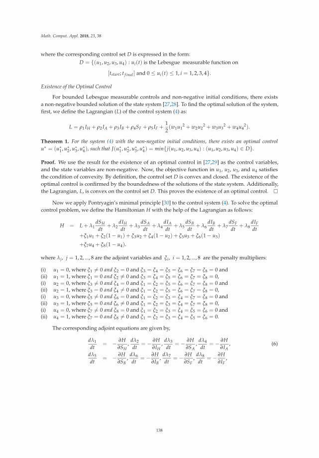
Math. Comput. Appl. 2018, 23, 38
where the corresponding control set D is expressed in the form:D = {(u1, u2, u3, u4) : ui(t) is the Lebesgue measurable function on
[tstart; t f inal ] and 0 ≤ ui(t) ≤ 1, i = 1, 2, 3, 4}.
Existence of the Optimal Control
For bounded Lebesgue measurable controls and non-negative initial conditions, there existsa non-negative bounded solution of the state system [27,28]. To find the optimal solution of the system,first, we define the Lagrangian (L) of the control system (4) as:
L = ρ1 IH + ρ2 IA + ρ3 IB + ρ4SF + ρ5 IF +12(w1u1
2 + w2u22 + w3u3
2 + w4u42).
Theorem 1. For the system (4) with the non-negative initial conditions, there exists an optimal controlu∗ = (u∗
1, u∗2, u∗
3, u∗4), such that J(u∗
1, u∗2, u∗
3, u∗4) = min{j(u1, u2, u3, u4) : (u1, u2, u3, u4) ∈ D}.
Proof. We use the result for the existence of an optimal control in [27,29] as the control variables,and the state variables are non-negative. Now, the objective function in u1, u2, u3, and u4 satisfiesthe condition of convexity. By definition, the control set D is convex and closed. The existence of theoptimal control is confirmed by the boundedness of the solutions of the state system. Additionally,the Lagrangian, L, is convex on the control set D. This proves the existence of an optimal control.
Now we apply Pontryagin’s minimal principle [30] to the control system (4). To solve the optimalcontrol problem, we define the Hamiltonian H with the help of the Lagrangian as follows:
H = L + λ1dSHdt
+ λ2dIHdt
+ λ3dSAdt
+ λ4dIAdt
+ λ5dSBdt
+ λ6dIBdt
+ λ7dSFdt
+ λ8dIFdt
+ξ1u1 + ξ2(1 − u1) + ξ3u2 + ξ4(1 − u2) + ξ5u3 + ξ6(1 − u3)
+ξ7u4 + ξ8(1 − u4).
where λj, j = 1, 2, ..., 8 are the adjoint variables and ξi, i = 1, 2, ..., 8 are the penalty multipliers:
(i) u1 = 0, where ξ1 = 0 and ξ2 = 0 and ξ3 = ξ4 = ξ5 = ξ6 = ξ7 = ξ8 = 0 and(ii) u1 = 1, where ξ1 = 0 and ξ2 = 0 and ξ3 = ξ4 = ξ5 = ξ6 = ξ7 = ξ8 = 0,(i) u2 = 0, where ξ3 = 0 and ξ4 = 0 and ξ1 = ξ2 = ξ5 = ξ6 = ξ7 = ξ8 = 0 and(ii) u2 = 1, where ξ3 = 0 and ξ4 = 0 and ξ1 = ξ2 = ξ5 = ξ6 = ξ7 = ξ8 = 0,(i) u3 = 0, where ξ5 = 0 and ξ6 = 0 and ξ1 = ξ2 = ξ3 = ξ4 = ξ7 = ξ8 = 0 and(ii) u3 = 1, where ξ5 = 0 and ξ6 = 0 and ξ1 = ξ2 = ξ3 = ξ4 = ξ7 = ξ8 = 0,(i) u4 = 0, where ξ7 = 0 and ξ8 = 0 and ξ1 = ξ2 = ξ3 = ξ4 = ξ5 = ξ6 = 0 and(ii) u4 = 1, where ξ7 = 0 and ξ8 = 0 and ξ1 = ξ2 = ξ3 = ξ4 = ξ5 = ξ6 = 0.
The corresponding adjoint equations are given by,
dλ1
dt= − ∂H
∂SH,
dλ2
dt= − ∂H
∂IH,
dλ3
dt= − ∂H
∂SA,
dλ4
dt= − ∂H
∂IA, (6)
dλ5
dt= − ∂H
∂SB,
dλ6
dt= − ∂H
∂IB,
dλ7
dt= − ∂H
∂SF,
dλ8
dt= − ∂H
∂IF,
138

Math. Comput. Appl. 2018, 23, 38
where
∂H∂SH
= −λ1(t)(
β(1 − η1u1)π IF(t)IH(t)
(SH(t) + IH(t))2 + μH
)+ λ2(t)
(β(1 − η1u1)
π IF(t)IH(t)(SH(t) + IH(t))2
)+λ7(t)
(β(1 − η4u4)
γSF(t)IH(t)(SH(t) + IH(t))2
)− λ8(t)
(β(1 − η4u4)
γSF(t)IH(t)(SH(t) + IH(t))2
),
∂H∂IH
= ρ1 + λ1(t)(
β(1 − η1u1)π IF(t)SH(t)
(SH(t) + IH(t))2
)− λ2(t)
(β(1 − η1u1)
π IF(t)SH(t)(SH(t) + IH(t))2 + μH
)−λ7(t)
(β(1 − η4u4)
γSF(t)(SH(t) + IH(t))2
)+ λ8(t)
(β(1 − η4u4)
γSF(t)(SH(t) + IH(t))2
),
∂H∂SA
= −λ3(t)(
α(1 − η2u2)ωIF(t)IA(t)
(SA(t) + IA(t))2 + μA
)+ λ4(t)
(α(1 − η2u2)
ωIF(t)IA(t)(SA(t) + IA(t))2
)+λ7(t)
(α(1 − η4u4)
κSF(t)IA(t)(SA(t) + IA(t))2
)− λ8(t)
(β(1 − η4u4)
κSF(t)IA(t)(SA(t) + IA(t))2
),
∂H∂IA
= ρ2 + λ3(t)(
α(1 − η2u2)ωIF(t)SA(t)
(SA(t) + IA(t))2
)− λ4(t)
(α(1 − η2u2)
ωIF(t)SA(t)(SA(t) + IA(t))2 + μA
)−λ7(t)
(α(1 − η4u4)
κSF(t)SA(t)(SA(t) + IA(t))2
)+ λ8(t)
(α(1 − η4u4)
κSF(t)SA(t)(SA(t) + IA(t))2
),
∂H∂SB
= −λ5(t)(
α(1 − η3u3)τIF(t)IB(t)
(SB(t) + IB(t))2 + μB
)+ λ6(t)(α(1 − η3u3)
τ IF(t)IB(t)(SB(t) + IB(t))2
)+λ7(t)
(α(1 − η4u4)
ζSF(t)IB(t)(SB(t) + IB(t))2
)− λ8(t)
(β(1 − η4u4)
ζSF(t)IB(t)(SB(t) + IB(t))2
), (7)
∂H∂IB
= ρ3 + λ5(t)(
α(1 − η3u3)τIF(t)SB(t)
(SB(t) + IB(t))2
)− λ6(t)(α(1 − η3u3)
τ IF(t)SB(t)(SB(t) + IB(t))2 + μB
)−λ7(t)
(α(1 − η4u4)
ζSF(t)SB(t)(SB(t) + IB(t))2
)+ λ8(t)
(β(1 − η4u4)
ζSF(t)SB(t)(SB(t) + IB(t))2
),
∂H∂SF
= ρ4 − λ7(t){
β(1 − η4u4)γIH(t)
(SH(t) + IH(t))− α(1 − η4u4)
κ IA(t)(SA(t) + IA(t))
−α(1 − η4u4)ζ IB(t)
(SB(t) + IB(t))− μF
}+ λ8(t){β(1 − η4u4)
γIH(t)(SH(t) + IH(t))
+α(1 − η4u4)κIA(t)
(SA(t) + IA(t))+ α(1 − η4u4)
ζ IB(t)(SB(t) + IB(t))
},
∂H∂IF
= ρ5 − λ1(t)β(1 − η1u1)πSH(t)
(SH(t) + IH(t))+ λ2(t)β(1 − η1u1)
πSH(t)(SH(t) + IH(t))
−λ3(t)α(1 − η2u2)ωSA(t)
(SA(t) + IA(t))+ λ4(t)α(1 − η2u2)
ωSA(t)(SA(t) + IA(t))
−λ5(t)α(1 − η3u3)τSB(t)
(SB(t) + IB(t))+ λ6(t)α(1 − η3u3)
τSB(t)(SB(t) + IB(t))
− λ8(t)μF.
139
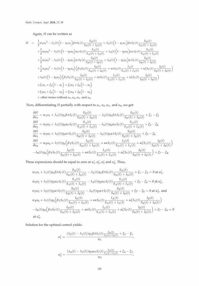
Math. Comput. Appl. 2018, 23, 38
Again, H can be written as
H =12
w1u12 − λ1(t)
(1 − η1u1
)βπ IF(t)
SH(t)SH(t) + IH(t)
+ λ2(t)(
1 − η1u1
)βπ IF(t)
SH(t)SH(t) + IH(t)
+12
w2u22 − λ3(t)
(1 − η2u2
)αωIF(t)
SA(t)SA(t) + IA(t)
+ λ4(t)(
1 − η2u2
)αωIF(t)
SA(t)SA(t) + IA(t)
+12
w3u32 − λ5(t)
(1 − η3u3
)ατ IF(t)
SB(t)SB(t) + IB(t)
+ λ6(t)(
1 − η2u2
)ατ IF(t)
SB(t)SB(t) + IB(t)
+12
w4u42 − λ7(t)
(1 − η4u4
)(βγSF(t)
IH(t)SH(t) + IH(t)
+ ακSF(t)IA(t
SA(t) + IA(t)+ αζSF(t)
IB(t)SB(t) + IB(t)
)+λ8(t)
(1 − η4u4
)(βγSF(t)
IH(t)SH(t) + IH(t)
+ ακSF(t)IA(t)
SA(t) + IA(t)+ αζSF(t)
IB(t)SB(t) + IB(t)
)+ξ1u1 + ξ2
(1 − u1
)+ ξ3u2 + ξ4
(1 − u2
)+ξ5u3 + ξ6
(1 − u3
)+ ξ7u4 + ξ8
(1 − u4
)+ other terms without u1, u2, u3, and u4.
Now, differentiating H partially with respect to u1, u2, u3, and u4, we get:
∂H∂u1
= w1u1 + λ1(t)η1βπ IF(t)SH(t)
SH(t) + IH(t)− λ2(t)η1βπ IF(t)
SH(t)SH(t) + IH(t)
+ ξ1 − ξ2
∂H∂u2
= w2u2 + λ3(t)η2αωIF(t)SA(t)
SA(t) + IA(t)− λ4(t)η2αωIF(t)
SA(t)SA(t) + IA(t)
+ ξ3 − ξ4
∂H∂u3
= w3u3 + λ5(t)η3ατ IF(t)SB(t)
SB(t) + IB(t)− λ6(t)η3ατ IF(t)
SB(t)SB(t) + IB(t)
+ ξ5 − ξ6
∂H∂u4
= w4u4 + λ7(t)η4
(βγSF(t)
IH(t)SH(t) + IH(t)
+ ακSF(t)IA(t)
SA(t) + IA(t)+ αζSF(t)
IB(t)SB(t) + IB(t)
)−λ8(t)η4
(βγSF(t)
IH(t)SH(t) + IH(t)
+ ακSF(t)IA(t)
SA(t) + IA(t)+ αζSF(t)
IB(t)SB(t) + IB(t)
)+ ξ7 − ξ8.
These expressions should be equal to zero at u∗1, u∗
2, u∗3 and u∗
4. Thus,
w1u1 + λ1(t)η1βπ IF(t)SH(t)
SH(t) + IH(t)− λ2(t)η1βπ IF(t)
SH(t)SH(t) + IH(t)
+ ξ1 − ξ2 = 0 at u∗1,
w2u2 + λ3(t)η2αωIF(t)SA(t)
SA(t) + IA(t)− λ4(t)η2αωIF(t)
SA(t)SA(t) + IA(t)
+ ξ3 − ξ4 = 0 at u∗2,
w3u3 + λ5(t)η3ατ IF(t)SB(t)
SB(t) + IB(t)− λ6(t)η3ατ IF(t)
SB(t)SB(t) + IB(t)
+ ξ5 − ξ6 = 0 at u∗3, and
w4u4 + λ7(t)η4
(βγSF(t)
IH(t)SH(t) + IH(t)
+ ακSF(t)IA(t)
SA(t) + IA(t)+ αζSF(t)
IB(t)SB(t) + IB(t)
)−λ8(t)η4
(βγSF(t)
IH(t)SH(t) + IH(t)
+ ακSF(t)IA(t)
SA(t) + IA(t)+ αζSF(t)
IB(t)SB(t) + IB(t)
)+ ξ7 − ξ8 = 0
at u∗4.
Solution for the optimal control yields:
u∗1 =
(λ2(t)− λ1(t))η1βπ IF(t)SH(t)
SH(t)+IH(t) + ξ2 − ξ1
w1,
u∗2 =
(λ4(t)− λ3(t))η2αωIF(t)SA(t)
SA(t)+IA(t)+ ξ4 − ξ3
w2,
140

Math. Comput. Appl. 2018, 23, 38
u∗3 =
(λ6(t)− λ5(t))η3ατ IF(t)SB(t)
SB(t)+IB(t)+ ξ6 − ξ5
w3, and
u∗4 =
(λ8(t)− λ7(t))η4
(βγSF(t)
IH(t)SH(t)+IH(t) + ακSF(t)
IA(t)SA(t)+IA(t)
+ αζSF(t)IB(t)
SB(t)+IB(t)
)+ ξ8 − ξ7
w4.
There are three cases to be considered for u∗1(t).
Case 1: 0 < u∗1 < 1, subject to the condition ξ1 = ξ2 = 0:
u∗1 =
(λ2(t)− λ1(t))η1βπ IF(t)SH(t)
SH(t)+IH(t)
w1. (8)
Case 2: u∗1 = 0, subject to the condition ξ1 = 0 and ξ2 = 0:
(λ2(t)− λ1(t))η1βπ IF(t)SH(t)
SH(t) + IH(t)= ξ1. (9)
Case 3: u∗1 = 1, subject to the condition ξ1 = 0 and ξ2 = 0:
(λ2(t)− λ1(t))η1βπ IF(t)SH(t)
SH(t) + IH(t)+ ξ2 = w1. (10)
Therefore, the optimal control u∗1(t) can be stated as:
u∗1 = max
(min
( (λ2(t)− λ1(t))η1βπIF(t)SH(t)
SH(t)+IH(t)
w1, 1)
, 0)
. (11)
There are also three cases to be considered for u∗2(t).
Case 1: 0 < u∗2 < 1, subject to the condition ξ3 = ξ4 = 0:
u∗2 =
(λ4(t)− λ3(t))η2αωIF(t)SA(t)
SA(t)+IA(t)
w2(12)
Case 2: u∗2 = 0, subject to the condition ξ3 = 0 and ξ4 = 0:
(λ4(t)− λ3(t))η2αωIF(t)SA(t)
SA(t) + IA(t)= ξ3. (13)
Case 3: u∗2 = 1, subject to the condition ξ3 = 0 and ξ4 = 0:
(λ4(t)− λ3(t))η2αωIF(t)SA(t)
SA(t) + IA(t)+ ξ4 = w2. (14)
Therefore, the optimal control u∗2(t) can be stated as:
u∗2 = max
(min
( (λ4(t)− λ3(t))η2αωIF(t)SA(t)
SA(t)+IA(t)
w2, 1)
, 0)
. (15)
There are three cases to be considered for u∗3(t).
141

Math. Comput. Appl. 2018, 23, 38
Case 1: 0 < u∗3 < 1, subject to the condition ξ5 = ξ6 = 0:
u∗3 =
(λ6(t)− λ5(t))η3ατIF(t)SB(t)
SB(t)+IB(t)
w3. (16)
Case 2: u∗3 = 0, subject to the condition ξ5 = 0 and ξ6 = 0:
(λ6(t)− λ5(t))η3ατ IF(t)SB(t)
SB(t) + IB(t)= ξ5. (17)
Case 3: u∗3 = 1, subject to the condition ξ5 = 0 and ξ6 = 0:
(λ6(t)− λ5(t))η3ατ IF(t)SB(t)
SB(t) + IB(t)+ ξ6 = w3. (18)
Therefore, the optimal control u∗3(t) can be stated as:
u∗3 = max
(min
( (λ6(t)− λ5(t))η3ατ IF(t)SB(t)
SB(t)+IB(t)
w3, 1)
, 0)
. (19)
There are also three cases to be considered for u∗4(t).
Case 1: 0 < u∗4 < 1, subject to the condition ξ7 = ξ8 = 0:
u∗4 =
(λ8(t)− λ7(t))η4
(βγSF(t)
IH(t)SH(t)+IH(t) + ακSF(t)
IA(t)SA(t)+IA(t)
+ αζSF(t)IB(t)
SB(t)+IB(t)
)w4
. (20)
Case 2: u∗4 = 0, subject to the condition ξ7 = 0 and ξ8 = 0:
(λ8(t)− λ7(t))η4
(βγSF(t)
IH(t)SH(t) + IH(t)
+ ακSF(t)IA(t)
SA(t) + IA(t)+ αζSF(t)
IB(t)SB(t) + IB(t)
)= ξ7. (21)
Case 3: u∗4 = 1, subject to the condition ξ7 = 0 and ξ8 = 0:
(λ8(t)− λ7(t))η4
(βγSF(t)
IH(t)SH(t) + IH(t)
+ ακSF(t)IA(t)
SA(t) + IA(t)+ αζSF(t)
IB(t)SB(t) + IB(t)
)+ ξ8 = w4. (22)
Therefore, the optimal control u∗4(t) can be stated as:
u∗4 = max
(min
( (λ8(t)− λ7(t))η4
(βγSF(t)
IH(t)SH(t)+IH(t)
+ ακSF(t)IA(t)
SA(t)+IA(t)+ αζSF(t)
IB(t)SB(t)+IB(t)
)w4
, 1)
, 0)
. (23)
Above, the optimal controls u∗1, u∗
2, u∗3, u∗
4 are functions of time t, and all the phase variables informulae (11), (15), (19), and (23) correspond to these optimal solutions of the state system (4).
4. Numerical Simulation
It is clear from Figure 4 that the susceptible population increased faster than the infectedpopulation when R0 < 1. This verifies that disease-free equilibrium existed if R0 < 1. In Figure 5,we plot the time series solutions of the model variables corresponding to susceptible human SH(t) andinfected human IH(t), susceptible animal Type A SA and infected animal Type A IA, susceptible animalType B SB and infected population Type B IB, and susceptible vector population SF(t) and infectedvector population IF(t) for different values of the model parameter that are depicted in Table 1. To findthe stability of the non-trivial equilibrium E∗, we chose initial values as E∗(S∗
H , I∗H , S∗A, I∗A, S∗
B, I∗B, S∗F, I∗F)
= (300, 50, 30, 20, 15, 8, 1500, 500). From Figure 5, we observe that the disease-free state did not exist if
142

Math. Comput. Appl. 2018, 23, 38
R0 > 1 and the system moved towards the endemic state. From the existence and stability analysis ofthe system, β, π, and τ seem to be important parameters. System dynamics of the model without drugapplication are shown in Figure 5. From Figure 5, it is also observed that when transmission factorπ = 0.18 and τ = 0.05 with β = 0.24 and μH = 0.1, the system went to an infected state condition.However, if β = 0.18, π = 0.16, and τ = 0.05, the system moved to an infection-free state and thedisease did not persist.
From Figure 6, we considered η1 = 0.2, η2 = 0.3, η3 = 0.1, and η4 = 0.4 as the efficacy of drugapplied in human, Type A animal, and Type B animal, and insecticide spray on the vector population,respectively [31]. Then, we observed the change of character for the infected human population,the infected reservoir populations (Types A and B), and the vector population due to control effects.The population of susceptible humans increased and also that of susceptible animals increased afterapplying control efforts, since the control (drug) effects decreased the contact rate between infectedflies and humans and also decrease the contact rate between infected vector and reservoir populations.This in turn restricted the spread of leishmaniasis.
Table 1. List of parameters.
Parameter Definition Range Default Value Reference
λH Recruitment rate of human population 300–318 317 [5]λF Recruitment rate of sand fly population 14,950–15,000 14,950 [5]λA Recruitment rate of animal population of Type A 70–150 73 [5]λB Recruitment rate of animal population of Type B 3–40 20 [32]μH Death rate of human population 0.000007–0.0001 0.00004 AssumedμF Death rate of sand fly population 0.188–0.795 0.189 [5]μA Death rate of animal population of Type A 0.06–0.21 0.19 [5]μB Death rate of animal population of Type B 0.089–0.255 0.25 [32]β Biting rate of sand fly on human 0.15–0.29 0.24 [5,9]α Biting rate of sand fly on animals of Type A and Type B 0.15–0.25 0.16 [5]π Transmission probability of CL in sand fly 0.12–0.24 0.18 [5,9]ω Transmission probability of CL on animal of Type A 0.11–0.172 0.12 [32]τ Transmission probability of CL on animal of Type B 0.02–0.071428 0.05 [5,9]γ Transmission probability of CL in sand fly from infected human 0.11–0.25 0.14 [5,9]κ Transmission probability of CL in sand fly from infected animal A 0.07–0.21 13 [5,9]ζ Transmission probability of CL in sand fly from infected animal B 0.04–0.21 0.12 [32]
Figure 4. Population densities of the model variables for R0 < 1 for disease-free state (all parametersare in Table 1).
143
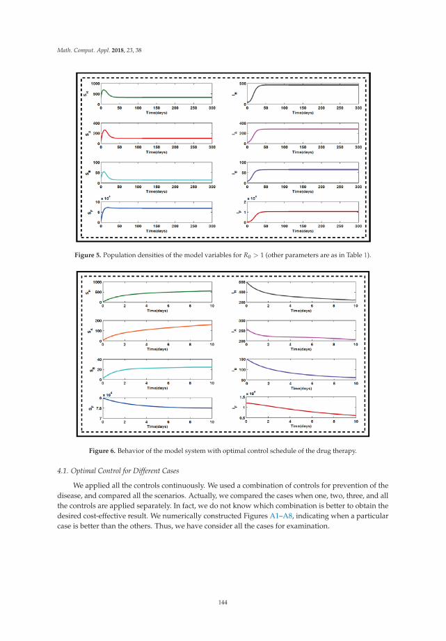
Math. Comput. Appl. 2018, 23, 38
Figure 5. Population densities of the model variables for R0 > 1 (other parameters are as in Table 1).
Figure 6. Behavior of the model system with optimal control schedule of the drug therapy.
4.1. Optimal Control for Different Cases
We applied all the controls continuously. We used a combination of controls for prevention of thedisease, and compared all the scenarios. Actually, we compared the cases when one, two, three, and allthe controls are applied separately. In fact, we do not know which combination is better to obtain thedesired cost-effective result. We numerically constructed Figures A1–A8, indicating when a particularcase is better than the others. Thus, we have consider all the cases for examination.
144

Math. Comput. Appl. 2018, 23, 38
We numerically investigated the effect of the following optimal controls on the spread ofleishmaniasis in a population for different cases [33,34].
• Case I: Prevention of the infection of animals Type A and Type B by the disease, along withspraying insecticides on the sand fly vectors.
• Case II: Prevention of animal Type B being infected by the disease, along with sprayinginsecticides on the sand fly vectors.
• Case III: Spraying insecticides on the sand fly vectors.• Case IV: Prevention of animal Type A being infected by the disease, along with spraying
insecticides on the sand fly vectors.• Case V: Prevention of animal Type B being infected by the disease, along with spraying
insecticides on the sand fly vectors.• Case VI: Prevention of humans being infected by the disease, along with spraying insecticides on
the sand fly vectors.• Case VII: Prevention of humans and animal Type A being infected by the disease, along with
spraying insecticides on the sand fly vectors.• Case VIII: Prevention of humans and animals Type A and Type B being infected by the disease,
along with spraying insecticides on the sand fly vectors.
See Appendix A.
4.2. Impact of Optimal Control on the Different Cases Proposed
We aimed to describe the long-term behavior of the disease prevalence for the future, which cannotbe predicted by the application of the optimal control strategies used in our model. After effectivestrategies are stopped, there are often some infectious people remaining who can cause a fresh outbreakof the disease [35]. Since the basic reproduction number proved to be effective in measuring long-termendemicity in [23], the effects of our applied strategies on (R0) were studied. Figure 7 demonstrates theresults of numerical simulation of (R0) under the various control strategy approaches. Assuming thatthe combinations of optimal control were implemented in the beginning of the year, it was observedthat case VIII performed well in the early stages, and also kept the disease under check. Cases I, VII, V,IV, II, VI, and III performed almost similarly throughout.
Figure 7. Effect of different control cases on R0 and magnified for t = 7.5–10 days.
145

Math. Comput. Appl. 2018, 23, 38
For longer time periods, R0 increased, at which point further application of control policiesbecomes necessary. Thus, the implementation of different strategies during different points of timeproduces different disease dynamics. Hence, it becomes important to determine the exact point intime at which the effective strategy needs to be implemented. Further, the complete elimination ofthe disease by effective application of the control strategy can be possible only if these strategies arecontinued over long time periods, by determination of the class boundaries of the controls u1, u2, u3,and u4.
Figure S3 describes the numerical simulation outcomes of R0 for the various cases of controlstrategies applied to each population.
4.3. Rescued Population and Vector Reduction for Different Cases
The useful data for finding rescued population-based strategy are in Table 2. The maximumnumber of humans were rescued within time in Cases VIII and VII, and the minimum number ofhumans were rescued in Cases III and II. The maximum number of infected animals of Type A wereextricated within time in Cases VII and VIII, and the minimum number of animals of Type A wereextricated in Case V. The maximum number of animals of Type B were rescued within time in CaseVIII, and the minimum number of animals of Type B were rescued in Cases III and IV. The maximumvector reduction occurred within time in Cases VIII and VII, followed by Case II, and the minimumreduction occurred in Case III. Therefore, we can say empirically that the maximum number of humanswere rescued in time when implementing Case VIII. Additionally, the maximum number of vectorswere reduced in time compared to the other strategies. However, this cannot be the most cost-effectiveapproach because of all of the drugs and insecticides which are applied to each of the populations tocontrol the disease.
Table 2. Reduction in infected host population (%).
Cases Human Animal A Animal B Vector Reduction
Case I 12.67 22.31 4.67 31.10Case II 12 11.15 4.67 29.7Case III 11.83 11.15 4.00 29.54Case IV 12.50 12.92 4.00 30.90Case V 18.16 5.17 4.67 31.54Case VI 18 11.92 4.67 31.38Case VII 18.5 23.07 4.67 32.75Case VIII 18.60 23.07 5.33 32.92
4.4. Cost-Effectiveness of the Different Cases
Herein, we consider the size of the population rescued from infection as well as the extent ofvector reduction with the different control strategies. For this, we assumed that the cost of the controlswere the square of the proportional to the number of controls deployed, and considered the costof drug u1 per person to be approximately 1.86$ (in INR 118.94) [36], the cost of drug u2 per TypeA animal to be 1.2$ (in INR 76.74), the cost of drug u3 per Type B animal to be 1$ (in INR 63.95),and the cost of insecticide spraying u4 per square meter area for vector death to be 1.5$ (in INR 95.92).The assumption was based on the understanding that the primary goal of using the drug is for thecure of those infected by the disease. Moreover, the use of insecticides is for the removal of vector.The difference between the total size of the infectious population without control and with controlwas used to determine the number of infections averted. We used the size of the rescued populationand extent of vector reduction, as depicted in Table 3. The control strategy applied in the model gavemaximum cost benefit. This was determined for each intervention strategy, illustrated in Figures 8and 9. One can see that the most cost-effective cases in terms of number of infections averted, includingthe number reduction of the sand fly vector, was the spraying of insecticides (Case III).
146
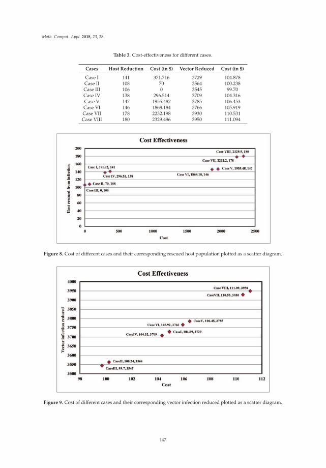
Math. Comput. Appl. 2018, 23, 38
Table 3. Cost-effectiveness for different cases.
Cases Host Reduction Cost (in $) Vector Reduced Cost (in $)
Case I 141 371.716 3729 104.878Case II 108 70 3564 100.238Case III 106 0 3545 99.70Case IV 138 296.514 3709 104.316Case V 147 1955.482 3785 106.453Case VI 146 1868.184 3766 105.919Case VII 178 2232.198 3930 110.531Case VIII 180 2329.496 3950 111.094
Figure 8. Cost of different cases and their corresponding rescued host population plotted as a scatter diagram.
Figure 9. Cost of different cases and their corresponding vector infection reduced plotted as a scatter diagram.
147

Math. Comput. Appl. 2018, 23, 38
4.5. Discussion
The disease leishmaniasis spreads from animal (reservoir) to human (host) via a vector. For thisreason, the control of vectors and infected reservoir populations is one of the most efficient approachesto exterminating the disease cutaneous leishmaniasis. Applying a suitable drug to the reservoirpopulation and spraying insecticide to kill the vector perform significant functions for controlling CL.We investigated the dynamics in the absence of drug applied in human hosts and animals, and withoutthe spraying of insecticide to kill the vector. The disease-free situation existed for R0 < 1. On theother hand, if R0 > 1, the disease-free state lost its stability and the system tended towards theendemic condition.
From Figure 5, we observe that susceptible human host population was sharply decreasedup to approximately 30 days, and the infected human host population gradually increased up toapproximately 30 days. Susceptible animal of Type A sharply decreased up to approximately 25 daysand susceptible animal of Type B sharply decreased up to approximately 20 days. Again, the infectedanimal population of Type A gradually increased up to approximately 25 days, and the population ofinfected animals of Type B gradually increased up to approximately 20 days. The susceptible sandfly population increased up to approximately 12 days, and the infected sand fly population graduallyincreased up to approximately 20 days. Thus, we can conclude that the disease can be controlled byinsecticide spraying with a frequency appropriate to the size of the vector population. The changeof the behavioral structure of the system dynamics depends on the biting rate and the transmissionpossibility of the sand fly. So, if we are able to kill the sand fly by spraying insecticide, then biting rateand transmission will automatically be reduced and then the disease can be controlled.
The inclusion of latent and recovered categories and the use of delayed terms in the modelequation system may change the dynamics of the disease. However, the life cycle of the parasite is notlong enough to support the incubation period. Therefore, we did not consider the latent status in ourmodel. Additionally, the progression from susceptible to infected classes passes through a latent stage.So, we ignored the intermediate stages (latent and recovered) and considered susceptible and infectedstages only. We paid no attention to the delay term, because our main aim was to control the infectedpopulation and the vector. Consequently, we considered the delay term to be in steady state.
The effectiveness of the drug dose influences the system to move towards the infection-free state.The results obtained from analytical and numerical simulations showed that the control strategieswere very effective if applied at the same time in the same region. The proposed optimal controlcan eradicate and prevent further transmission of the disease through the vector. Although totaleradication of cutaneous leishmaniasis seems complicated in a realistic environment, if our findingscan be applied to an infected zone, then a pioneering insight can be achieved against cutaneousleishmaniasis in a global perspective.
To prevent vector-borne disease, different strategic cases can be applied to a finite time period.The effects of the different cases used to minimize the disease among the various populationswere investigated using the analysis of optimal control, thereby depicting the real situations.Herein, we considered four controls upon three types of mammalian host and a vector population:prevention of infective individuals by using drugs and spraying of insecticides to kill vector. It wasdeduced that the strategy applied in Case I yielded good results for a considerable time period,however Case III was most cost effective but did not achieve as great a reduction in infected host orvector in the same time period. For the entire period of the preventive measure, the effects of ourcontrol strategies on R0 were observed to determine the effects of the controls on the future spreadof disease. The significant changes in the number of possible secondary infections from an infectedindividual were thus concluded to be dependent on time. Thus, it becomes important to determine theexact time interval during which the optimal control must be applied. Moreover, it is only possible toeliminate the disease entirely if the different control strategies are continued for a long duration inthe future.
148

Math. Comput. Appl. 2018, 23, 38
5. Conclusions
From the study of the effects of the various control cases on R0, it was observed that Case VIIIyielded the best results in attempting to control the disease, followed by Cases VII and V. The analysisof cost-effectiveness indicated that Case III was the most cost-effective, followed by Case II. Thoughthe potential of Case I in trying to eliminate the disease is comparatively better than that of CaseIV, it involves higher costs. It can be concluded that the cases which display low disease prevalencewould require an efficient and cost-effective strategy (Cases II and IV). However, the cases where theutmost priority is to control the disease would require strategic cases that are less cost-effective but actefficiently to control the disease in a short time period (e.g., Case I). Hence, our model would suffice inassisting decisions related to the allocation of resources, where the fundamental aim is to select thebest strategy to eliminate the disease in the lowest possible time.
Supplementary Materials: Supplementary materials are available online: http://www.mdpi.com/2078-2489/23/3/38/s1.
Author Contributions: Model Formulation, problem observation, and its solution were generated by professorE.V.G. and professor P.K.R. Mathematical analysis, numerical simulation, as well as most of the work in thismanuscript were realistically done by the research scholar D.B. Comprehensive progression of the solution wasdone by the research scholars S.D. and J.C.
Acknowledgments: The research is supported by the PURSE-DST, Department of Mathematics, JadavpurUniversity, Government of India.
Conflicts of Interest: The authors declare no conflict of interest.
Appendix A
• Case I: Optimal Use of Drug for Prevention From Disease for Animals Type A and Type B with Spray ofInsecticides on Vector
In this case, the objective function J is optimized by the preventive control measures u2, u3,and the control involving spraying of insecticides u4, while u1 (the control parameter for humans)is set to zero. We observed in Figure A1 that due to the control strategies, the number of infectedhumans IH decreased. A similar decrease was observed in infected animals of Types A and B. Infectedvector population also decreased due to the inclusion of spraying insecticide in the control strategy,while an increased number was observed for the case without control. In this case, infected human IHwas reduced by 12.67%, infected animal A was reduced by 22.13%, infected animal B was reducedby 4.67%, and vector death rate was reduced by 31.10%. Therefore, almost 100% rescued cases wasachieved for humans in 78 days, for animal Type A in 45 days, and animal Type B in 200 days,and vector was removed in 32 days. From Figure A1, we find that the controls u2 and u4 were initially100%, following which u2 slowly dropped to the lower bound after 9.7 days. Moreover, the control u4
dropped to the lower bound after 9.85 days. Here the control u3 was 100% effective almost from thefirst day and reached the lower bound in almost the seventh day. Hence, the control effect of u2 wasnear the optimum level but the spray of insecticide for this strategy showed the actual optimal level.
149

Math. Comput. Appl. 2018, 23, 38
Figure A1. The behavior of the model system with control and without control for Case I foru1 = 0 and u2 = u3 = u4 = 0.
• Case II: Optimal Use of Drug for Prevention of Disease for Animal Type B with Spray of Insecticideson Vector
In this case, control parameters for preventive measure u3 and u4 were used to optimize theobjective function J, while the other control parameters for prevention u1, u2 were zero. We observedin Figure A2 that due to the control strategies, the number of infected humans IH decreased. A similardecrease was observed in infected animals of Types A and B. Additionally, the infected vectorpopulation decreased due to the inclusion of spraying insecticide in the control strategy, while anincreased number was observed for the case without control. For this case, infected human IH wasreduced by 12%, infected animal A was reduced by 11.15%, infected animal B was reduced by 4.67%,and vector death was 29.7%. Therefore, almost 100% rescued cases were achieved for humans in80 days, for animal Type A in 89 days, animal Type B in 200 days, and vector was removed in33 days. From Figure A2, it is evident that the control u3 was initially 100% at around 0.65 days, afterwhich control trajectory u3 decreased slowly in the lower level almost 7 days. Moreover, the controlu4 was initially 100% effective from the beginning and decreased to the lower bound after 9.8 days.Therefore, insecticide spray was almost effective most of the days, and for that reason the number ofvectors removed was optimal compared to the other controls for this strategy.
Figure A2. The behavior of the model system with control and without control for Case II foru1 = u2 = 0 and u3 = u4 = 0.
150

Math. Comput. Appl. 2018, 23, 38
• Case III: Optimal Use of Spray of Insecticides on the Sand Fly Vector
In order to optimize the objective function J, this policy involves only control via sprayinginsecticides u4, while we fixed the controls for preventive measure u1, u2, and u3 to zero. We observedin Figure A3 that due to the control strategies, the number of infected humans IH decreased. A similardecrease was observed in infected animals of Types A and B. Also, the infected vector populationdecreased due to the inclusion of spraying insecticide in the control strategy, while an increasednumber was observed for the case without control. In this case, infected human IH was reduced by11.83%, infected animal Type A was reduced by 11.15%, infected animal Type B was reduced by 4%,and vector death was 29.54%. Therefore, almost 100% rescued cases were achieved for humans in80 days, for animal Type A in 89 days, animal Type B in 250 days, and vector was removed in 33 days.From Figure A3, we find that the control u4 was initially 100%, following which it slowly dropped tothe lower bound after 9.97 days. Therefore, effect of insecticide spray lasts longer compared to theother cases.
Figure A3. The behavior of the model system with control and without control for Case III foru1 = u2 = u3 = 0 and u4 = 0.
• Case IV: Optimal Use of Drug for Prevention from Disease for Animal Type A with Spray of Insecticideson Vector
In this case, the control for preventive measure u2 is applied along with the control with thespraying of insecticides u4, with the aim of optimizing the objective function J, and we fixed thecontrols for preventive control parameter u1 and u3 to zero. We observed in Figure A4 that due to thecontrol strategies, the number of infected humans IH decreased. A similar decrease was observed ininfected animals of Types A and B. Also, the infected vector population decreased due to the inclusionof spraying insecticide in the control strategy, while an increased number was observed for the casewithout control. For this case, infected human IH was reduced by 12.5%, infected animal Type Awas reduced by 12.92%, infected animal Type B was reduced by 4%, and vector death was 30.90%.Therefore, almost 100% rescued cases was achieved for humans in 76 days, for animal Type A in76 days, animal Type B in 250 days, and vector was removed in 32 days. From Figure A4, we find thatthe controls u2 and u4 were initially 100%, following which u2 and u4 slowly dropped to the lowerbound after 9.7 days. Moreover, the control u4 dropped to the lower bound after 9.9 days. Hence thecontrol u2 and u4 were effective for almost the maximum time span. However, the control u4 wasslightly better than the other controls.
151

Math. Comput. Appl. 2018, 23, 38
Figure A4. The behavior of the model system with control and without control for Case IV foru1 = u3 = 0 and u2 = u4 = 0.
• Case V: Optimal Use of Drug for Prevention from Disease for Human and Animal Type B with Spray ofInsecticides on Vector
In this case, the preventive measure for controls u1 and u3, along with the spraying of insecticidesu4, are applied with the aim of optimizing the objective function J, and we fixed the control for theprevention of animal Type A u2 to zero. We observed in Figure A5 that due to these control strategies,the number of infected humans IH decreased. A similar decrease was observed in infected animalsof Types A and B. Also, the infected vector population decreased due to the inclusion of sprayinginsecticide in the control strategy, while an increased number was observed for the case without control.In this case, infected human IH was reduced by 18.16%, infected animal Type A was reduced by 5.17%,infected animal Type B was reduced by 4.67%, and vector mortality was 31.54%. Therefore, almost100% rescue cases was achieved for humans in 55 days, for animal Type A in 153 days, animal Type Bin 200 days, and vector was removed in 31 days. From Figure A5, we find that the controls u1 and u4
were initially 100% , following which they slowly dropped to the lower bound after 9.3 days, whilecontrol u4 dropped to lower bound after 9.9 days. The control u3 was at 100%, almost from 0.7 days atthe beginning, and reached the lower bound after 7 days. Therefore, once spraying is complete, it stayson for the maximum time, yielding the maximum benefit under this strategy.
Figure A5. The behavior of the model system with control and without control for Case V for u2 = 0and u1 = u3 = u4 = 0.
152
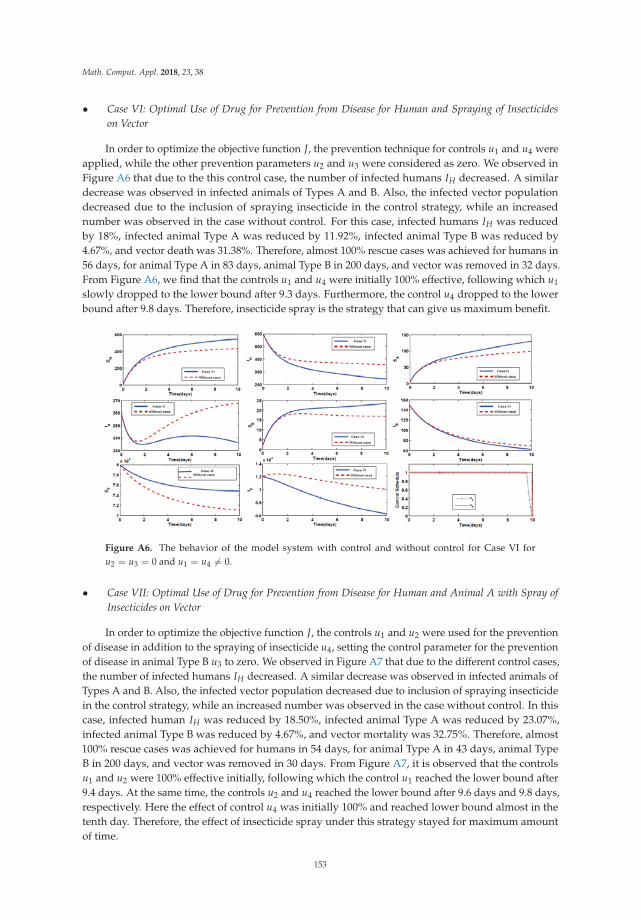
Math. Comput. Appl. 2018, 23, 38
• Case VI: Optimal Use of Drug for Prevention from Disease for Human and Spraying of Insecticideson Vector
In order to optimize the objective function J, the prevention technique for controls u1 and u4 wereapplied, while the other prevention parameters u2 and u3 were considered as zero. We observed inFigure A6 that due to the this control case, the number of infected humans IH decreased. A similardecrease was observed in infected animals of Types A and B. Also, the infected vector populationdecreased due to the inclusion of spraying insecticide in the control strategy, while an increasednumber was observed in the case without control. For this case, infected humans IH was reducedby 18%, infected animal Type A was reduced by 11.92%, infected animal Type B was reduced by4.67%, and vector death was 31.38%. Therefore, almost 100% rescue cases was achieved for humans in56 days, for animal Type A in 83 days, animal Type B in 200 days, and vector was removed in 32 days.From Figure A6, we find that the controls u1 and u4 were initially 100% effective, following which u1
slowly dropped to the lower bound after 9.3 days. Furthermore, the control u4 dropped to the lowerbound after 9.8 days. Therefore, insecticide spray is the strategy that can give us maximum benefit.
Figure A6. The behavior of the model system with control and without control for Case VI foru2 = u3 = 0 and u1 = u4 = 0.
• Case VII: Optimal Use of Drug for Prevention from Disease for Human and Animal A with Spray ofInsecticides on Vector
In order to optimize the objective function J, the controls u1 and u2 were used for the preventionof disease in addition to the spraying of insecticide u4, setting the control parameter for the preventionof disease in animal Type B u3 to zero. We observed in Figure A7 that due to the different control cases,the number of infected humans IH decreased. A similar decrease was observed in infected animals ofTypes A and B. Also, the infected vector population decreased due to inclusion of spraying insecticidein the control strategy, while an increased number was observed in the case without control. In thiscase, infected human IH was reduced by 18.50%, infected animal Type A was reduced by 23.07%,infected animal Type B was reduced by 4.67%, and vector mortality was 32.75%. Therefore, almost100% rescue cases was achieved for humans in 54 days, for animal Type A in 43 days, animal TypeB in 200 days, and vector was removed in 30 days. From Figure A7, it is observed that the controlsu1 and u2 were 100% effective initially, following which the control u1 reached the lower bound after9.4 days. At the same time, the controls u2 and u4 reached the lower bound after 9.6 days and 9.8 days,respectively. Here the effect of control u4 was initially 100% and reached lower bound almost in thetenth day. Therefore, the effect of insecticide spray under this strategy stayed for maximum amountof time.
153

Math. Comput. Appl. 2018, 23, 38
Figure A7. The behavior of the model system with control and without control for Case VII for u3 = 0and u1 = u2 = u4 = 0.
• Case VIII: Optimal Use of Drug for Prevention from Disease for Human, Animals Type A and Type Bwith Spraying of Insecticides on Vector
In this case, in order to optimize the objective function J, all four controls (i.e., u1, u2, u3, and u4)were used. After comparison of Case VIII with the circumstance when no controls were applied,it could be concluded that while the human population which was susceptible increased in number,the infected human population decreased, which is illustrated in Figure A8. It was also observed in thiscase that in general, two types of susceptible animal populations increased in number and the infectedsand fly populations decreased remarkably at an almost exponential rate. In particular, the sand flypopulation reduced below 3000 in around 10 days. The comparison at t = 10 days shows that therewas an increase by 113 individuals in SH , decrease by 60 individuals in IA, and IB and IF by 8 and3950 individuals, respectively. With the help of this strategic case, infected human IH was reduced by18.60%, infected animal Type A was reduced by 23.07%, infected animal Type B was reduced by 5.33%,and vector mortality was 32.92%. Therefore, almost 100% rescue cases was achieved for humans in53 days, for animal Type A in 43 days, animal Type B in 187, days and vector was removed in 30 days.Figure A8 shows that the control u1 was 100% effective initially, following which it dropped slowly tothe lower bound after 9.5 days. At the same time, the controls u2 and u3 reached the lower bound after9.3 days and 7 days, respectively. The control u4 was initially 100% effective and reached the lowerbound at approximately the tenth day. It can be concluded that a low amount of insecticide spray isnecessary in this strategy.
Figure A8. The behavior of the model system with control and without control for Case VIII foru1 = u2 = u3 = u4 = 0.
154

Math. Comput. Appl. 2018, 23, 38
References
1. Sharma, U.; Singh, S. Immunobiology of leishmaniasis. Indian J. Exp. Biol. 2009, 47, 412–423. [PubMed]2. Park, K. Preventive and Social Medicine; Banarsidas Bhanot Publishers: Jabalpur, India, 2005.3. Chaves, L.F.; Hernandez, M.J. Mathematical modelling of American Cutaneous Leishmaniasis: Incidental
hosts and threshold conditions for infection persistence. Acta Trop. 2004, 92, 245–252. [CrossRef] [PubMed]4. World Health Organization. Leishmaniasis. Fact Sheet Updated April 2017. Available online: http://www.
who.int/news-room/fact-sheets/detail/leishmaniasis (accessed on 18 July 2018).5. ELmojtaba, I.M.; Mugisha, J.Y.T.; Hashim, M.H.A. Mathematical analysis of the dynamics of visceral
leishmaniasis in the Sudan. Appl. Math. Comput. 2010, 217, 2567–2578. [CrossRef]6. Kassiri, H.; Sharifinia, N.; Jalilian, M.; Shemshad, K. Epidemiological aspects of cutaneous leishmaniasis in
Ilam province, west of Iran (2000–2007). Asian Pac. J. Trop. Dis. 2012, 2, S382–S386. [CrossRef]7. Reithinger, R.; Dujardin, J.C.; Louzir, H.; Pirmez, C.; Alexander, B.; Brooker, S. Cutaneous leishmaniasis.
Lancet Infect. Dis. 2007, 7, 581–596. [CrossRef]8. Kasper, D.L.; Braunwald, E.; Fauci, A.S.; Hauser, S.L.; Longo, D.L.; Jameson, J.L.; Loscalzo, J. Harrison’s
Principles of Internal Medicine, 17th ed.; McGraw-Hill: New York, NY, USA, 2008; Volume 1, Chapter 1–216.9. Bathena, K. A Mathematical Model of Cutaneous Leishmaniasis. Master’s Thesis, Rochester Institute of
Technology, Rochester, NY, USA, 2009.10. Miller, E.; Huppert, A. The effects of Host Diversity on Vector-Borne Disease: The Conditions under Which
Diversity Will Amplify or Dilute the Disease Risk. PLoS ONE 2013, 8, e80279. [CrossRef] [PubMed]11. Jaouadi, K.; Haouas, N.; Chaara, D.; Gorcii, M.; Chargui, N.; Augot, D.; Pratlong, F.; Dedet, J.P.;
Ettlijani, S.; Mezhoud, H.; et al. First detection of Leishmania killicki (Kinetoplastida, Trypanosomatidae) inCtenodactylus gundi (Rodentia, Ctenodactylidae), a possible reservoir of human cutaneous leishmaniasis inTunisia. Parasites Vectors 2011, 4, 159. [CrossRef] [PubMed]
12. Chatterjee, A.N.; Roy, P.K.; Mondal, J. Mathematical Model for Suppression of Sand Flies through IRS withDDT in Visceral Leishmaniasis. Am. J. Math. Sci. 2013, 2, 105–112.
13. Wu, H.J.J.; Massad, E. Mathematical modelling for Zoonotic Visceral Leishmaniasis dynamics: A newanalysis considering updated parameters and notified human Brazilian data. Infect. Dis. Model. 2017,2, 143–160.
14. Bacaer, N.; Guernaoui, S. The epidemic threshold of vector-borne diseases with seasonality the case ofcutaneous leishmaniasis in Chichaoua, Morocco. J. Math. Biol. 2006, 53, 421–436. [CrossRef] [PubMed]
15. Biswas, D.; Kesh, D.K.; Datta, A.; Chatterjee, A.N.; Roy, P.K. A Mathematical Approach to Control CutaneousLeishmaniasis Through Insecticide Spraying. Sop Trans. Appl. Math. 2014, 1, 44–54. [CrossRef]
16. Biswas, D.; Roy, P.K.; Li, X.Z.; Basir, F.A.; Pal, J. Role of macrophage in the disease dynamics of cutaneousleishmaniasis: A delay induced mathematical study. Commun. Math. Biol. Neurosci. 2016, 2016, 1–31.
17. Roy, P.K.; Li, X.Z.; Biswas, D.; Datta, A. Impulsive Application to Design Effective Therapies AgainstCutaneous Leishmaniasis Under Mathematical Perceptive. Commun. Math. Biol. Neurosci. 2017, 2017, 1–17.
18. Biswas, D.; Datta, A.; Roy, P.K. Combating Leishmaniasis through Awareness Campaigning: A MathematicalStudy on Media Efficiency. Int. J. Math. Eng. Manag. Sci. 2016, 1, 139–149.
19. Zamir, M.; Zaman, G.; Alshomrani, A.S. Sensitivity Analysis and Optimal Control of AnthroponoticCutaneous Leishmania. PLoS ONE 2016, 11, e0160513. [CrossRef] [PubMed]
20. Begon, M.; Bennett, M.; Bowers, R.G.; French, N.P.; Hazel, S.M.; Turner, J. A clarication of transmission termsin host-microparasite models: numbers, densities and areas. Epidemiol. Infect. 2002, 129, 147–153. [CrossRef][PubMed]
21. Abubakar, A.; Ruiz-Postigo, A.J.; Pita, J.; Lado, M.; Ben-Ismail, R.; Argaw, D.; Alvar, J. Visceral leishmaniasisoutbreak in South Sudan 2009–2012: Epidemiological assessment and impact of a multisectoral response.PLoS Negl. Trop Dis. 2014, 8, e2720. [CrossRef] [PubMed]
22. Subramanian, A.; Singh, V.; Sarkar, R.R. Understanding Visceral Leishmaniasis Disease Transmission and itsControl—A Study Based on Mathematical Modeling. Mathematics 2015, 3, 913–944. [CrossRef]
23. Biswas, S.; Subramanian, A.; ELMojtaba, I.M.; Chattopadhyay, J.; Sarkar, R.R. Optimal combinations ofcontrol strategies and cost-effective analysis for visceral leishmaniasis disease transmission. PLoS ONE 2017,12, e0172465. [CrossRef] [PubMed]
155

Math. Comput. Appl. 2018, 23, 38
24. Brett-Major, D.M.; Claborn, D.M. sandfly Fever: What Have We Learned in One Hundred Years? Mil. Med.2009, 174, 426–431. [CrossRef] [PubMed]
25. Rogers, M.E.; Bates, P.A. Leishmania Manipulation of sandfly Feeding Behavior Results in EnhancedTransmission. PLoS Pathog. 2007, 3, e91. [CrossRef] [PubMed]
26. Lopez, L.F.; Coutinho, F.A.B.; Burattini, M.N.; Massad, E. Threshold conditions for infection persistence incomplex host-vectors interactions. Comptes Rendus Biol. 2002, 325, 1073–1084. [CrossRef]
27. Zaman, G.; Kang, Y.H.; Jung, I.H. Stability analysis and optimal vaccination of an SIR epidemic model.BioSystems 2008, 93, 240–249. [CrossRef] [PubMed]
28. Birkhoff, G.; Rota, G.C. Ordinary Differential Equations, 4th ed.; John Wiley and Sons: New York, NY, USA, 1989.29. Lukes, D.L. Differential Equations: Classical to Controlled in Mathematics in Science and Engineering; Academic
Press: New York, NY, USA, 1982; Volume 162.30. Kirschner, D.; Lenhart, S.; Serbin, S. Optimal control of the chemotherapy of HIV. J. Math. Biol. 1997, 35,
775–792. [CrossRef] [PubMed]31. Shimozako, H.J.; Wu, J.; Massad, E. The Preventive Control of Zoonotic Visceral Leishmaniasis: Efficacy and
Economic Evaluation. Comput. Math. Methods Med. 2017, 2017, 4797051. [CrossRef] [PubMed]32. Kaabi, B.; Ahmed, S.B. Assessing the effect of zooprophylaxis on zoonotic cutaneous leishmaniasis
transmission: A system dynamics approach. Biosystems 2013, 114, 253–260. [CrossRef] [PubMed]33. Okosuna, K.O.; Rachid, O.; Marcus, N. Optimal control strategies and cost-effectiveness analysis of a malaria
model. BioSystems 2013, 111, 83–101. [CrossRef] [PubMed]34. Sardar, T.; Mukhopadhyay, S.; Bhowmick, A.R.; Chattopadhyay, J. An optimal cost effectiveness study on
Zimbabwe cholera seasonal data from 2008–2011. PLoS ONE 2013, 8, e81231. [CrossRef] [PubMed]35. Stauch, A.; Sarkar, R.R.; Picado, A.; Ostyn, B.; Sundar, S.; Rijal, S.; Boelaert, M.; Dujardin, J.; Duerr, H. Visceral
Leishmaniasis in the Indian Subcontinent: Modelling Epidemiology and Control. PLoS Negl. Trop. Dis.2011, 5, e1405. [CrossRef] [PubMed]
36. Costs of Medicines in Current Use for the Treatment of Leishmaniasis (Annex6), Drug Prices(January 2010). Available online: http://www.who.int/leishmaniasis/research/978_92_4_12_949_6_Annex6.pdf (accessed on 18 July 2018).
c© 2018 by the authors. Licensee MDPI, Basel, Switzerland. This article is an open accessarticle distributed under the terms and conditions of the Creative Commons Attribution(CC BY) license (http://creativecommons.org/licenses/by/4.0/).
156

Mathematical
and Computational
Applications
Article
Optimal Control and Computational Method for theResolution of Isoperimetric Problem in aDiscrete-Time SIRS System
Fadwa El Kihal , Imane Abouelkheir, Mostafa Rachik and Ilias Elmouki *
Department of Mathematics and Computer Sciences, Faculty of Sciences Ben M’Sik,Hassan II University of Casablanca, Casablanca 20000, Morocco; [email protected] (F.E.K.);[email protected] (I.A.); [email protected] (M.R.)* Correspondence: [email protected]
Received: 7 September 2018; Accepted: 22 September 2018; Published: 24 September 2018
Abstract: We consider a discrete-time susceptible-infected-removed-susceptible “again” (SIRS)epidemic model, and we introduce an optimal control function to seek the best control policyfor preventing the spread of an infection to the susceptible population. In addition, we definea new compartment, which models the dynamics of the number of controlled individuals and whoare supposed not to be able to reach a long-term immunity due to the limited effect of control.Furthermore, we treat the resolution of this optimal control problem when there is a restriction onthe number of susceptible people who have been controlled along the time of the control strategy.Further, we provide sufficient and necessary conditions for the existence of the sought optimalcontrol, whose characterization is also given in accordance with an isoperimetric constraint. Finally,we present the numerical results obtained, using a computational method, which combines the secantmethod with discrete progressive-regressive schemes for the resolution of the discrete two-pointboundary value problem.
Keywords: discrete-time model; SIRS model; optimal control; isoperimetric problem
1. Introduction
Many mathematical models in epidemiology are used to assist in finding the most appropriatecontrol strategies for a given group of individuals who belong to different classes. These classesare often represented in epidemic systems, using compartments that are usually named susceptible(S), exposed (E), infectious or infected (I) and removed or recovered (R) [1]. In this paper, we areinterested in the study of a population infected by an epidemic and whose dynamics are describedusing a discrete-time SIRS system. The SIRS models in the continuous-time case have been widelystudied by many researchers as in [2], where Acedo et al. proposed an analytical approach to find theexact global solution of the classical SIRS epidemic system. Furthermore, there are Alexander andMoghadas in [3] and Hu et al. in [4], who all provided bifurcation analysis of the SIRS model withdifferent incidence rates. The authors who contributed with Teng in [5] and in [6] found significantresults from the study of the persistence and extinction of disease using SIRS models. As for Jin et al.in [7], Liu and Zhou in [8] and Chen in [9], they obtained stability conditions for other SIRS systems.A stability analysis of the SIRS model in the discrete-time case is not often available, but there existinteresting analyses done for some classes of this type of model; see for example, the work of Hu et al.in [10]. As an application of such models in a particular case of disease, Mukhopadhyay and Tapaswipublished their paper about Japanese encephalitis in [11]. Other authors studied SIRS dynamics whenthe model framework was in the form of a discrete metapopulation-like system [12].
Math. Comput. Appl. 2018, 23, 52; doi:10.3390/mca23040052 www.mdpi.com/journal/mca157

Math. Comput. Appl. 2018, 23, 52
In parallel, there are many researchers who have benefited from modeling approaches inepidemics, in order to determine the best prevention strategies against the spread of infection tosusceptibles, using different optimization techniques such as optimal control methods; see examplesin [13–20]. On the other hand, some models as in [21–23] discussed the impact of limited public healthresources in the propagation of infectious diseases, but there are very few optimization problemsthat have been adapted to such subjects. Here, we try to resolve this issue by exploiting studiespublished in [24–26], where medical constraints have been modeled differently with a constraint called“isoperimetric”. More precisely, we propose an anti-epidemic control strategy that targets susceptiblepeople, under the isoperimetric condition that we could not control all individuals of this category dueto restricted health resources.
We consider a simple discrete-time epidemic compartmental model devised in the form ofdifference equations, which describe the dynamics of a discrete-time SIRS model with a temporarycontrolled class, meaning that the controlled people cannot acquire long-lived immunity to movetowards the removed compartment due to the temporary effect of the control parameter. Thereafter,we characterize the sought optimal control, and we show the effectiveness of this limited control policy.This optimal control problem leads to the execution of two numerical methods all combined togetherat the same time, namely the forward-backward sweep method to generate the optimal state andcontrol functions and the secant method adapted to the isoperimetric restriction.
2. Materials
Let us define a discrete-time model with the four following main compartments:
• S: the number of susceptible people to infection or who are not yet infected,• CS: the number of susceptible people who are temporarily controlled, so they cannot move
to the removed class due to the limited effect of control. It can represent the compartment ofvaccinated people in case a vaccination is not 100% effective due to the difficulty of producinga perfect vaccine, the heterogeneity of the population or a vaccine not conferring a lifelongimmunity [17,27],
• I: the number of infected people who are capable of spreading the epidemic to those in thesusceptible and temporarily controlled categories,
• R: the number of removed people from the epidemic, but can return to the susceptible classbecause of the short-term removal individuals’ immunity.
In our modeling approach, we aim to describe the dynamics of variables S, CS, I and R at time ibased on the following difference equations:⎧⎪⎪⎪⎨⎪⎪⎪⎩
Si+1 = Si − βSi Ii − aθiSi + Πi − μSi + σRiCSi+1 = CSi + aθiSi − bβCSi Ii − μCSi
Ii+1 = Ii + β(Si + bCSi )Ii − γIi − μIiRi+1 = Ri + γIi − μRi − σRi
(1)
with initial conditions S0 > 0, CS0 ≥ 0, I0 ≥ 0 and R0 ≥ 0 and where Πi = μNi with Ni =
Si + CSi + Ii + Ri, gives the newborn people, aθ (0 ≤ a ≤ 1) is the recruitment rate of susceptiblesto the controlled class with θ defining the control parameter as a constant between 0 and 1 (see suchconsideration in the case of vaccination in [27]) and “a” modeling the reduced chances of a susceptibleindividual to be controlled, β = δ
Niwith δ the infection transmission rate, μ the natural death rate,
bθ (0 ≤ b ≤ 1) the recruitment rate of controlled people to the infected class even in the presence of θ
with “b” modeling the reduced chances of a temporarily controlled individual to be infected, γ therecovery rate and σ the losing removal individuals’ immunity rate. We note that the population size Niis constant at any time i because Ni+1 = Si+1 + CSi+1 + Ii+1 + Ri+1 = Ni. Hence, Πi = Π = constant.
158

Math. Comput. Appl. 2018, 23, 52
3. Methods
Now, we consider the mathematical model (1) with θ as a discrete control function.Motivated by the desire to reduce the number of infected people as much as possible while
minimizing the value of the control θ over N times, our objective is to seek an optimal control θ∗
such that:
J(θ∗) = minθ∈Θ
J(θ) (2)
where J is the functional defined by:
J(θ) =N−1
∑i=0
(AIi +
B2
θ2i
)+ AIN (3)
and where the control space Θ is defined by the set:
Θ = {θ ∈ RN |θmin ≤ θi ≤ θmax, θmax ≤ 1 θmin ≥ 0, i = 0, ..., N − 1}}
A and B represent constant severity weights associated with functions I and θ, respectively.Managers of the anti-epidemic resources cannot well predict whether their control strategy will
reach all the susceptible population over N times. To model the situation in which a restricted resourceof control is available, we consider that the number of susceptible people we can control is equal to aconstant C > 0 for N days. Hence, we try to find θ∗ under the definition of the following isoperimetricrestriction:
C =N−1
∑i=0
aθiSi (4)
In [25,26], the authors defined an isoperimetric constraint on the control variable only, to model thetotal tolerable dosage amount of a therapy along the treatment period. In their conferences talks [28,29],Kornienko et al. and de Pinho et al. introduced state constraints in an optimal control problem that issubject to an S-exposed-I-Rdifferential system to model the situation of the limited supply of vaccinebased on the work in [24] and where the isoperimetric constraint is defined on the product of thecontrol and state variables. Our study aims to highlight more the importance of such optimal controlapproaches by considering a discrete model rather than a continuous one. This would be interestingsince data are often collected at discrete times, as noted in [30].
In our case, to take into account the constraint (4) for the resolution of the optimal controlproblem (2), we consider a new variable Z defined as:
Zi+1 = Zi + aθiSi (5)
with Z0 = 0 and ZN = C.The discrete-time system of (1) becomes:⎧⎪⎪⎪⎪⎪⎨⎪⎪⎪⎪⎪⎩
Si+1 = Si + Π − βSi Ii − aθiSi − μSi + σRiCSi+1 = CSi + aθiSi − bβCSi Ii − μCSi
Ii+1 = Ii + β(Si + bCSi )Ii − γIi − μIiRi+1 = Ri + γIi − μRi − σRiZi+1 = Zi + aθiSi
(6)
In the following, we announce two theorems for proving the existence and the characterization ofthe sought optimal control θ∗.
Theorem 1. (Sufficient conditions) For the isoperimetric optimal control problem given by (2) along with thediscrete state equations in (6), there exists a control θ∗ ∈ Θ such that J(θ∗) = minθ∈Θ J(θ).
159

Math. Comput. Appl. 2018, 23, 52
Proof. In order to prove the existence of a solution θ∗ in Θ, we try to prove that minθ∈Θ J(θ) exists.We have a finite number of time steps N and discrete state equations in System (6) with bounded
coefficients γ, μ, b, σ, Π, a and β, then for all θ in the control set Θ, the N-component state variables:
S = (S0, S1, ..., Si, ..., SN−1),
CS = (CS0 , CS1 , ..., CSi , ..., CSN−1),
I = (I0, I1, ..., Ii, ..., IN−1)
and R = (R0, R1, ..., Ri, ..., RN−1) ∀i = 0, ..., N − 1
are uniformly bounded, which implies that ∀θ ∈ Θ, J(θ) is uniformly bounded.We can deduce then that in fθ∈Θ J(θ) is finite since J(θ) is bounded, and there exists a finite number
j of uniformly bounded sequences θ j ∈ Θ such that limj→∞ J(θ j) = in fθ∈Θ J(θ) and corresponding
sequences of states Sj, CjS, I j and Rj.
Thus, there exists θ∗ ∈ Θ and S∗, C∗S, I∗, R∗ ∈ RN such that on a subsequence,
θ j → θ∗,
Sj → S∗,
CjS → C∗
S,
I j → I∗
and Rj → R∗.
Finally, due to the finite dimensional structure of the system (6) and the objective function J(θ),θ∗ is an optimal control with corresponding states S∗, C∗
S, I∗ and R∗ [26]. Therefore, taking into accountthe structure of J being a convex function, in fθ∈Θ J(θ) is achieved.
In order to derive the necessary conditions of optimality, we employ the discrete version ofPontryagin’s maximum principle stated in Theorem A1 in Appendix A.
Theorem 2. (Necessary conditions) Given the optimal control θ∗ and solutions S∗, C∗S, I∗ and R∗, there exist
λl,i, l = 1, ..., 5, i = 0, ..., N, the adjoint variables satisfying the following equations:
�λ1,i = λ1,i+1(−1 + βI∗i + μ + aθ∗i )− aλ2,i+1θ∗i − βλ3,i+1 I∗i − aθ∗i λ5,i+1 (7)
�λ2,i = λ2,i+1(−1 + bβI∗i + μ)− bλ3,i+1βI∗i (8)
�λ3,i = −A + λ1,i+1βS∗i + bλ2,i+1βC∗
Si− λ3,i+1(−1 + β(S∗
i + bC∗Si)− μ − γ) (9)
−λ4,i+1γ
�λ4,i = λ4,i+1(μ + σ − 1)− σλ1,i+1 (10)
�λ5,i = −λ5,i+1 (11)
with �λl,i = λl,i+1 − λl,i, l = 1, ..., 5, i = 0, ..., N − 1 the difference operator and λ1,N = λ2,N = λ4,N = 0,λ3,N = A and λ5,N = constant to be determined, as the transversality conditions associated with adjointEquations (7)–(11).
In addition, the optimal control θ∗ is characterized at each iteration i by:
θ∗i = min(
max(
θmin,aS∗
i (λ1,i+1 − λ2,i+1 − λ5,i+1)
B
), θmax
)∀i = 0, ..., N − 1 (12)
Proof. With the application of a discrete version of Pontryagin’s maximum principle in Appendix Aand as done in [26,31,32], we can determine the discrete optimal control θ∗ for the problem (6) and itsassociated trajectories S∗, C∗
S, I∗ and R∗.
160

Math. Comput. Appl. 2018, 23, 52
We define a discrete Hamiltonian Hi as a brief notation of the function H defined for i = 0, ..., N − 1.as follows:
H(i, Si, CSi , Ii, Ri, λ1,i+1, λ2,i+1, λ3,i+1, λ4,i+1, λ5,i+1, θi)
= AIi +B2
θ2i + λ1,i+1Si+1 + λ2,i+1CSi+1 + λ3,i+1 Ii+1 + λ4,i+1Ri+1 + λ5,i+1Zi+1
The discrete-time adjoint system is resolved using the following formulations:
�λ1,i = −∂Hi∂Si
,�λ2,i = − ∂Hi∂CSi
,�λ3,i = −∂Hi∂Ii
,�λ4,i = −∂Hi∂Ri
and �λ5,i = −∂Hi∂Zi
that we associate with the following transversality conditions:
λ1,N =∂φN∂SN
, λ2,N =∂φN∂CSN
, λ3,N =∂φN∂IN
, λ4,N =∂φN∂RN
with φN representing the payoff term function in (3), namely AIN .Then, we obtain the following discrete-time adjoint system:⎧⎪⎪⎪⎪⎨⎪⎪⎪⎪⎩
�λ1,i = λ1,i+1(−1 + βIi + μ + aθi)− aλ2,i+1θi − βλ3,i+1 Ii − aθiλ5,i+1�λ2,i = λ2,i+1(−1 + bβIi + μ)− bλ3,i+1βIi�λ3,i = −A + λ1,i+1βSi + bλ2,i+1βCSi − λ3,i+1(−1 + β(Si + bCSi )− μ − γ)− λ4,i+1γ
�λ4,i = λ4,i+1(μ + σ − 1)− σλ1,i+1�λ5,i = −λ5,i+1
with the transversality conditions λ1,N = 0, λ2,N = 0, λ4,N = 0, λ3,N = A and λ5,N is unknown.In order to find the transversality condition λ5,N = constant, we use the secant-method as the
appropriate numerical technique for finding the zero of the function λ5,N → V(λ5,N) = ZN − ZN whereZN is the value of Z at final iteration N for various values of λ5,N and ZN is the value fixed by C [25,33].
Since θi is a bounded control, we can then define a Lagrangian L as follows:
L((i, Si, CSi , Ii, Ri, λ1,i+1, λ2,i+1, λ3,i+1, λ4,i+1, λ5,i+1, θi, ω1,i, ω2,i)
= Hi + ω1,i(θmax − θi) + ω2,i(θi − θmin)
where ω1,i, ω2,i ≥ 0 ∀i verifying at θi = θ∗i , the two conditions ω1,i(θmax − θ∗i ) = 0 and ω2,i(θ∗i −
θmin) = 0.Let Li be the brief notation of L and L∗
i be the brief notation of L at S∗, C∗S, I∗, R∗ and θ∗.
The condition of minimization is defined as:
L∗i = min
θi∈ΘLi(
∗∗).
In order to find the solution θ∗i of (∗∗), we differentiate the Lagrangian Li with respect to θi on theset Θ to obtain the optimality equation:
∂Li∂θi
= Bθi + aSi(λ2,i+1 − λ1,i+1) + aSiλ5,i+1 − ω1,i + ω2,i = 0 at θ∗i .
Furthermore, we find
θ∗i =aS∗
i (λ1,i+1 − λ2,i+1 − λ5,i+1)− ω2,i + ω1,i
B.
161

Math. Comput. Appl. 2018, 23, 52
If:
θmin < θ∗i < θmax,
then:
ω1,i = ω2,i = 0,
therefore:
θ∗i =aS∗
i (λ1,i+1 − λ2,i+1 − λ5,i+1)
B.
If:
θ∗i = θmin,
then:
ω1,i = 0,
therefore:
θmin =aS∗
i (λ1,i+1 − λ2,i+1 − λ5,i+1)− ω2,i
B,
implying that:
ω2,i = a (S∗i (λ1,i+1 − λ2,i+1)− S∗
i λ5,i+1)− Bθmin.
Knowing that ω2,i ≥ 0 and B > 0, we obtain θ∗i ≤ aS∗i (λ1,i+1 − λ2,i+1 − λ5,i+1)
B.
If:
θ∗i = θmax,
then:
ω2,i = 0,
thus:
θmax =aS∗
i (λ1,i+1 − λ2,i+1 − λ5,i+1) + ω1,i
B,
implying that ω1,k = Bθmax − a(S∗
i (λ1,i+1 − λ2,i+1)− S∗i λ5,i+1
).
Knowing that ω1,i ≥ 0 and B > 0, we obtain θ∗i ≥ aS∗i (λ1,i+1 − λ2,i+1 − λ5,i+1)
B.
Using these standard optimality arguments, we characterize the control u∗k by:
θ∗i =
⎧⎪⎪⎪⎪⎪⎪⎪⎨⎪⎪⎪⎪⎪⎪⎪⎩
aS∗i (λ1,i+1−λ2,i+1−λ5,i+1)
B if θmin <aS∗
i (λ1,i+1−λ2,i+1−λ5,i+1)B < θmax
θmin if aS∗i (λ1,i+1−λ2,i+1−λ5,i+1)
B ≤ θmin
θmax if aS∗i (λ1,i+1−λ2,i+1−λ5,i+1)
B ≥ θmax
162

Math. Comput. Appl. 2018, 23, 52
or by a more reduced form, we can write
θ∗i = min(
max(
θmin,aS∗
i (λ1,i+1 − λ2,i+1 − λ5,i+1)
B
), θmax
)4. Numerical Results and Discussion
In this section, we resolve the discrete two-point value problem defined by System (6) withinitial conditions along with Equations (7)–(11) with final conditions, using a discrete version of theforward-backward sweep method (FBSM) [26,33] with the incorporation of a discrete progressiveiterative scheme to stock at each iteration i, the values of the state variables corresponding tothe forward discrete-time system (6), to use them in a second discrete regressive iterative schemeincorporated for stocking at each time i, the values of the adjoint state variables corresponding to thebackward discrete-time adjoint system (7)–(11). In fact, at each time i, the values stocked of both stateand adjoint state variables were utilized in the characterization of the optimal control θ∗. In brief,our algorithm is defined by the following four steps of numerical calculus (Algorithm 1).
Algorithm 1: Resolution steps of the discrete two-point boundary value optimal controlproblem (6)–(11).
Step 0:Guess an initial estimation of θ.
Step 1:Use the initial condition S(0), CS(0), I(0), R(0) and Z(0) and the stocked values by θ.Find the optimal states S∗, C∗
S, I∗, R∗ and Z∗, which iterate forward in the discrete two-pointboundary value problem (6).
Step 2:Use the stocked values by θ and the transversality conditions λl,N+1 for l = 1, 2, 3, 4 while
searching the constant λ5,N+1 using the secant-method. More precisely, the secant method is used toobtain the zero of the function λ5,N → V(λ5,N) = ZN − ZN where ZN is the value of Z at finaliteration N for various values of λ5,N, and ZN is the value fixed by C. In addition, due its structurein (4), we choose the constant C in a way that it cannot exceed an upper bound N0 × N where N0 isthe initial population size and N is the number of iterations.
Find the adjoint variables λl for l = 1, 2, 3, 4, 5, which iterate backward in the discrete two-pointboundary value problem (6).
Step 3:Update the control utilizing new S, CS, I, R, Z and λl for l = 1, 2, 3, 4, 5 in the characterization of
θ∗ as presented in (12).Step 4:
Test the convergence. If the values of the sought variables in this iteration and the final iteration aresufficiently small, check out the recent values as solutions. If the values are not small, go back to Step 1.
Figure 1 depicts the behavior of the number of susceptible people in the absence and presenceof the control, and we can see that the number of susceptible people had decreased from its initialcondition once the control had been introduced, while there was no significant decrease of the Sfunction compared to the case when there was yet no control. With these parameters used, it reachedonly three people because of the maximal value of one taken by the optimal control θ∗ in almostalltimes of the control strategy, as seen in the last figure.
In Figure 2, we can well understand the increase of the number of the removed people becauseof a natural recovery, but it cannot represent a significant recovery because it has not reached even14 people, and this means that only a very small number of people have been removed based on theinitial condition I(0) considered. In the presence of the control, the R function increased towards
163

Math. Comput. Appl. 2018, 23, 52
a much higher number of removed people and showed it can even reach more than 31 individualsrecovered from the disease in the first 17 days; this number decreased thereafter because of the resultsin the next figure, which will show that infection will disappear as we move forward in time.
0 10 20 30 40 500
10
20
30
40
50
60
time (in days)
S
0 10 20 30 40 5054.85
54.9
54.95
55
time (in days)
S
Zoom of S without control
without controlwith control
Figure 1. Number of susceptible people in the absence and presence of the control in the two casesθ = 0 and θ = 0. Parameter values: Π = μN0, a = 0.5, b = 0.1, β = 10−5, μ = 0.00045, γ = 0.75× 10⁻²,σ = 5 × 10⁻⁴. Initial conditions: S(0) = 55, CS(0) = 0, I(0) = 42, R(0) = 0. Severity weight constants:A = 1 and B = 4 × 10⁵.
0 10 20 30 40 500
5
10
15
20
25
30
35
time (in days)
R
without controlwith control
Figure 2. Number of removed people in the absence and presence of the control in the two cases θ = 0and θ = 0, with the same parameter values, initial conditions and severity weights as in Figure 1.
164

Math. Comput. Appl. 2018, 23, 52
In Figure 3, the simulation shows that the number of infected people could decrease only becauseof a natural recovery or death, while the infection was still serious and remained present in morethan 28 individuals. After the introduction of the control, the I function started to decrease once theanti-epidemic was followed, and it tended to zero values after 37 days; this means most people wouldrecover from the disease at the end of the control strategy.
0 10 20 30 40 500
5
10
15
20
25
30
35
40
45
time (in days)
I
without controlwith control
Figure 3. Number of infected people in the absence and presence of the control in the two cases θ = 0and θ = 0, with the same parameter values, initial conditions and severity weights as in Figure 1.
As regards Figure 4, we sought to verify the condition C = 110, which meets the value 2 × S0,and we presented associated simulations of the number of controlled people, which increased to53 individuals once the optimal control had been introduced and increased thereafter, again showingthat it could even exceed that number, approximately towards 80 people when we go forward towardsthe end. In the same figure, we show the values of the optimal control θ∗, which take the value of oneas the maximal peak for almost alldays, and we can also see that the imposed isoperimetric constanthas been verified in the final instant with some error ε = 3.6589. In fact, it is not evident that it reachedany imposed value while verifying convergence tests of both methods used. Sometimes, the programdid not stop iterating or could not show the plot because of a NANvalue, and then, the only solutionwas to fix the number of iterations of the secant method in which the imposed initial guess of C wasapproximately reached.
In Figure 5, we exhibit the value of the sought constant missing transversality condition λ5,N ,which will be essential to verify the necessary conditions announced in Theorem 2. As we can observefrom this figure, the value obtained equals −1.3830 × 10⁸.
Figure 6 presents a numerical simulation of the Z function when we did not seek the verificationof the condition ZN = C, and we let ZN free, so we could prove that our algorithm in the case of theisoperimetric constraint helped to approximate ZN to C or even verify the equality between them,far from the value that could reach ZN when it was free; as we can see from the mentioned figure,ZN = 105.5729, which led to an important error of about 4.4271 from C that was sought in Figure 4.
165

Math. Comput. Appl. 2018, 23, 52
0 10 20 30 40 500
10
20
30
40
50
60
70
80
time (in days)
CS
0 10 20 30 40 500
0.2
0.4
0.6
0.8
1
time (in days)
θ*
0 10 20 30 40 500
20
40
60
80
100
120
time (in days)
Z
C−ε=106.3411
Figure 4. Number of controlled people, the optimal control θ∗ and the variable Z with an imposedconstant C = 110, with the same parameter values, initial conditions and severity weights as in Figure 1.
0 10 20 30 40 50−2
−1.9
−1.8
−1.7
−1.6
−1.5
−1.4
−1.3
−1.2
−1.1
−1x 10
8
time (in days)
λ5,
N
λ5,N
= −1.3830×10⁸
Figure 5. Value of the sought transversality condition λ5,N .
166

Math. Comput. Appl. 2018, 23, 52
0 10 20 30 40 500
20
40
60
80
100
120
time (in days)
Z
ZN
=105.5729
Figure 6. Z function when ZN is free and not forced to equal C.
5. Conclusions
In this paper, an optimal control approach with an isoperimetric constraint has been applied to adiscrete-time SIRS model, which was in the form of a four-compartmental epidemic model where itwas supposed that the controlled population did not reach the removed class due to the temporaryeffect of the control. The isoperimetric restriction, which has been proposed to define the number ofsusceptible people who receive the control along the anti-epidemic measures period, allowed us tofind the optimal control needed to fight against a disease when there were limited resources.
Author Contributions: All authors contributed equally to this work. All authors read and approved thefinal manuscript.
Acknowledgments: The authors would like to thank all the members of the Editorial Board who were responsiblefor dealing with this paper and the anonymous referees for their valuable comments and suggestions, improvingthe content of this paper.
Conflicts of Interest: The authors declare no conflict of interest.
Appendix A
Let us define the following:
• I: the set {0, ..., N − 1}• Xi: the real n-component column vector; i = 0, ..., N
167

Math. Comput. Appl. 2018, 23, 52
• θi: the real m-component column control vector; i = 0, ..., N − 1• Θ = {θ ∈ RN |θmin ≤ θi ≤ θmax, θmax ≤ 1 θmin ≥ 0, i = 0, .., N − 1}}: the set of
admissible controls• f : Rn × Rm × Θ → Rn, F : Rn × Rm × I → R, φ : Rm × I ∪ {N} → R, continuously
differentiable functions.
Let us consider a discrete-time optimal control problem over times 0, ..., N, defined by:
min{J} =N−1
∑i=0
F(Xi, θi, i) + φ(XN , N) (A1)
subject to the discrete-time system:
Xi+1 = Xi + f (Xi, θi, i), i = 0, ..., N − 1 (A2)
X0 given (A3)
θi ∈ Θ (A4)
We now define the Hamiltonian function Hi to be:
Hi = H(Xi, θi, i) = F(Xi, θi, i) + λi+1 f (Xi, θi, i)
and in the optimal control and state by H∗i = H(X∗
i , θ∗i , i).Then, based on results of the discrete version of the maximum principle discussed in [34], we can
derive the following necessary conditions for our problem (A1) based on the following theorem.
Theorem A1. (A discrete version of the maximum principle) Given a discrete optimal control θ∗i in thesense of sufficient conditions and given solutions X∗
i , then the necessary conditions for θ∗i to be optimal forProblem (A1)–(A4) are:
X∗i+1 = X∗
i + f (X∗i , θ∗i , i), X0 given
Δλi = −∂H∗i
∂Xi, λN =
∂φ(X∗N , N)
∂XN
H∗i ≤ H(X∗
i , θi, i)
for all θ∗i ∈ Θ
References
1. Kermack, W.O.; McKendrick, A.G. A Contribution to the Mathematical Theory of Epidemics. Proc. R. Soc. A1927, 115, 700–721. [CrossRef]
2. Acedo, L.; González-Parra, G.; Arenas, A.J. An exact global solution for the classical SIRS epidemic model.Nonlinear Anal. Real World Appl. 2010, 11, 1819–1825. [CrossRef]
3. Alexander, M.E.; Moghadas, S.M. Bifurcation analysis of an SIRS epidemic model with generalized incidence.SIAM J. Appl. Math. 2005, 65, 1794–1816. [CrossRef]
4. Hu, Z.; Bi, P.; Ma, W.; Ruan, S. Bifurcations of an SIRS epidemic model with nonlinear incidence rate.Discret. Contin. Dyn. Syst. Ser. B 2011, 15, 93–112.
5. Teng, Z.; Liu, Y.; Zhang, L. Persistence and extinction of disease in non-autonomous SIRS epidemic modelswith disease-induced mortality. Nonlinear Anal. Theory Methods Appl. 2008, 69, 2599–2614. [CrossRef]
6. Xamxinur, A.; Teng, Z. On the persistence and extinction for a non–autonomous SIRS epidemic model.J. Biomath. 2006, 21, 167–176.
7. Jin, Y.; Wang, W.; Xiao, S. An SIRS model with a nonlinear incidence rate. Chaos Solitons Fractals 2007,34, 1482–1497.
168

Math. Comput. Appl. 2018, 23, 52
8. Liu, J.; Zhou, Y. Global stability of an SIRS epidemic model with transport-related infection.Chaos Solitons Fractals 2009, 40, 145–158.
9. Chen, J. An SIRS epidemic model. Appl. Math. J. Chin. Univ. 2004, 19, 101–108.10. Hu, Z.; Teng, Z.; Jiang, H. Stability analysis in a class of discrete SIRS epidemic models. Nonlinear Anal. Real
World Appl. 2012, 13, 2017–2033. [CrossRef]11. Mukhopadhyay, B.B.; Tapaswi, P.K. An SIRS epidemic model of Japanese encephalitis. Int. J. Math. Math. Sci.
1994, 17, 347–355. [CrossRef]12. Abouelkheir, I.; El Kihal, F.; Rachik, M.; Zakary, O.; Elmouki, I. A multi-regions SIRS discrete epidemic
model with a travel-blocking vicinity optimal control approach on cells. Br. J. Math. Comput. Sci. 2017, 20,1–16. [CrossRef] [PubMed]
13. Zakary, O.; Rachik, M.; Elmouki, I. On the impact of awareness programs in HIV/AIDS prevention: An SIRmodel with optimal control. Int. J. Comput. Appl. 2016, 133. [CrossRef]
14. Zakary, O.; Larrache, A.; Rachik, M.; Elmouki, I. Effect of awareness programs and travel-blocking operationsin the control of HIV/AIDS outbreaks: A multi-domains SIR model. Adv. Differ. Equ. 2016, 2016, 169.[CrossRef]
15. Shim, E. A note on epidemic models with infective immigrants and vaccination. Math. Biosci. Eng. 2006,3, 557. [CrossRef] [PubMed]
16. Roy, P.K.; Saha, S.; Al Basir, F. Effect of awareness programs in controlling the disease HIV/AIDS: An optimalcontrol theoretic approach. Adv. Differ. Equ. 2015, 2015, 217. [CrossRef]
17. Rodrigues, H.S.; Monteiro, M.T.T.; Torres, D.F. Vaccination models and optimal control strategies to dengue.Math. Biosci. 2014, 247, 1–12. [CrossRef] [PubMed]
18. Kumar, A.; Srivastava, P.K. Vaccination and treatment as control interventions in an infectious disease modelwith their cost optimization. Commun. Nonlinear Sci. Numer. Simul. 2017, 44, 334–343. [CrossRef]
19. Liu, X.; Takeuchi, Y.; Iwami, S. SVIR epidemic models with vaccination strategies. J. Theor. Biol. 2008,253, 1–11. [CrossRef] [PubMed]
20. Nainggolan, J.; Supian, S.; Supriatna, A.K.; Anggriani, N. Mathematical model of tuberculosis transmissionwith reccurent infection and vaccination. In Journal of Physics: Conference Series; IOP Publishing: Bristol, UK,2013; Volume 423, No. 1, p. 012059.
21. Zhou, L.; Fan, M. Dynamics of an SIR epidemic model with limited medical resources revisited.Nonlinear Anal. Real World Appl. 2012, 13, 312–324. [CrossRef]
22. Abdelrazec, A.; Bélair, J.; Shan, C.; Zhu, H. Modeling the spread and control of dengue with limited publichealth resources. Math. Biosci. 2016, 271, 136–145. [CrossRef] [PubMed]
23. Yu, T.; Cao, D.; Liu, S. Epidemic model with group mixing: Stability and optimal control based on limitedvaccination resources. Commun. Nonlinear Sci. Numer. Simul. 2018, 61, 54–70. [CrossRef]
24. Neilan, R.M.; Lenhart, S. An Introduction to Optimal Control with an Application in Disease Modeling.In Modeling Paradigms and Analysis of Disease Trasmission Models; American Mathematical Society: Providence,RI, USA, 2010; pp. 67–82.
25. Elmouki, I.; Saadi, S. BCG immunotherapy optimization on an isoperimetric optimal control problem for thetreatment of superficial bladder cancer. Int. J. Dyn. Control 2016, 4, 339–345. [CrossRef]
26. Alkama, M.; Rachik, M.; Elmouki, I. A discrete isoperimetric optimal control approach for BCGimmunotherapy in superficial bladder cancer: Discussions on results of different optimal doses. Int. J. Appl.Comput. Math. 2017, 3, 1–18. [CrossRef]
27. Sharomi, O.; Malik, T. Optimal control in epidemiology. Ann. Oper. Res. 2017, 251, 55–71. [CrossRef]28. Kornienko, I.; Paiva, L.T.; De Pinho, M.D.R. Introducing state constraints in optimal control for health
problems. Procedia Technol. 2014, 17, 415–422. [CrossRef]29. De Pinho, M.D.R.; Kornienko, I.; Maurer, H. Optimal control of a SEIR model with mixed constraints and L 1
cost. In Proceedings of the 11th Portuguese Conference on Automatic Control, CONTROLO’2014, Porto,Portugal, 21–23 July 2014; Springer: Cham, Switzerland, 2015; pp. 135–145.
30. Zakary, O.; Rachik, M.; Elmouki, I. On the analysis of a multi-regions discrete SIR epidemic model:An optimal control approach. Int. J. Dyn. Control 2017, 5, 917–930. [CrossRef]
31. Zakary, O.; Rachik, M.; Elmouki, I.; Lazaiz, S. A multi-regions discrete-time epidemic model with atravel-blocking vicinity optimal control approach on patches. Adv. Differ. Equ. 2017, 2017, 120. [CrossRef]
169

Math. Comput. Appl. 2018, 23, 52
32. Zakary, O.; Rachik, M.; Elmouki, I. A new epidemic modeling approach: Multi-regions discrete-time modelwith travel-blocking vicinity optimal control strategy. Infect. Dis. Model. 2017, 2, 304–322. [CrossRef][PubMed]
33. Lenhart, S.; Workman, J.T. Optimal Control Applied to Biological Models; CRC Press: Boca Raton, FL, USA, 2007.34. Sethi, S.P.; Thompson, G.L. What Is Optimal Control Theory? Springer: New York, NY, USA, 2000; pp. 1–22.
c© 2018 by the authors. Licensee MDPI, Basel, Switzerland. This article is an open accessarticle distributed under the terms and conditions of the Creative Commons Attribution(CC BY) license (http://creativecommons.org/licenses/by/4.0/).
170
Article
Solution of Optimal Harvesting Problem by FiniteDifference Approximations of Size-StructuredPopulation Model
Johanna Pyy 1,* ID , Anssi Ahtikoski 2, Alexander Lapin 3 and Erkki Laitinen 1
1 Faculty of Sciences, University of Oulu, FI-90014 Oulu, Finland; [email protected] Natural Resources Institute Finland (Luke) Oulu, FI-90014 Oulu, Finland; [email protected] Institute of Computational Mathematics & Information Technology, Kazan Federal University,
420008 Kazan, Russia; [email protected]* Correspondence: [email protected]
Received: 11 April 2018; Accepted: 24 April 2018 ; Published: 26 April 2018
Abstract: We solve numerically a forest management optimization problem governed by a nonlinearpartial differential equation (PDE), which is a size-structured population model. The formulatedproblem is supplemented with a natural constraint for a solution to be non-negative. PDE isapproximated by an explicit or implicit in time finite difference scheme, whereas the cost function istaken from the very beginning in the finite-dimensional form used in practice. We prove the stabilityof the constructed nonlinear finite difference schemes on the set of non-negative vectors and thesolvability of the formulated discrete optimal control problems. The gradient information is derivedby constructing discrete adjoint state equations. The projected gradient method is used for findingthe extremal points. The results of numerical testing for several real problems show good agreementwith the known results and confirm the theoretical statements.
Keywords: size-structured population model; nonlinear partial differential equation; finite differenceapproximation; optimization; gradient method
1. Introduction
The well-posedness of the continuous size-structured model has been studied in several papers(e.g., [1–4]). In Ref. [1], authors proved the local existence and uniqueness of a solution of the continuousmodel, where birth and mortality functions depend on total population. In Ref. [2], the authorsestablished the local existence and uniqueness of a solution of the size-structured nonlinear populationmodel, where also growth rate depends on total population. In the papers [3,4], the authors provedglobal existence and uniqueness of a solution of the continuous nonlinear population model, where allvital rates depend on total population. The total population can be described by e.g., total number ofindividuals (e.g., [3]), total biomass (e.g., [5]) or basal area.
A continuous nonlinear size-structured population model has been used in a forest managementoptimization problem (e.g., [6–8]). In a continuous formulation, this nonlinear optimization problemcannot be solved by analytic methods. A natural approach is to solve this problem by approximatinga continuous model by a discrete one and further solving a discrete optimization problem by iterativealgorithms. In this paper, we focus on development of finite difference schemes to approximate thesolution of a continuous nonlinear population model. Efficient schemes are essential for solvingoptimal control problems or parameter estimation problems as such problems require solving themodel numerous times before an optimal solution is obtained.
When continuous population model is approximated by a finite difference scheme, it becomesa matrix population model [9]. In matrix models, trees are divided into classes with respect to their
Math. Comput. Appl. 2018, 23, 22; doi:10.3390/mca23020022 www.mdpi.com/journal/mca171

Math. Comput. Appl. 2018, 23, 22
size—for instance, diameter. The matrix describes how the class division changes at one time step.Matrix population models have also been used for forest management optimizations (e.g., [10,11]).
In optimization, using iterative algorithms is inevitable. Higher-order algorithms are usuallysensitive to the regularity of the solution, and, therefore, they usually yield a convergence rate offirst order as soon as the compatibility conditions are not satisfied. Moreover, in practice, the vitalrates are determined on a statistical basis and the compatibility conditions required for high-orderconvergence are hardly valid with real-life data. These suggest that, in most cases, a first-order methodshould be the most adequate. Hence, it is desirable to have a robust scheme that can produce manyuseful qualitative and quantitative properties of the solutions of the differential problem but requiresminimum regularity of the solution [12]. Unfortunately, one could not derive the explicit formula forthe optimal strategy since the strategy, the state and the costate are coupled into a complex system.The results at this stage may be regarded as a middle step to real world applications and serve asa starting point for numerical computations [13].
In our knowledge, the comprehensive theoretical investigation of the forest managementoptimization problem with a continuous nonlinear population model as the state equation is stilllacking, and, in that sense, the problem is an open problem. Hence, in this work, the investigation ofthe problem in its differential form is omitted, whereas, we consider the finite dimensional counterpartof the problem constructed by finite difference approximations of the state problem and taking forcost function a finite dimensional form used in practice. We prove the stability of constructed finitedifference schemes on the set of non-negative solutions and solvability of the optimization problem,and deduce the necessary gradient information for iterative solution methods. We solve severalapplied problems, where different approximations schemes are used, and compare the computedresults. The rest of the article is organized as follows. In Section 2, a mathematical model of optimalharvesting problem for the size-structured forest is formulated. In Section 3, we construct andinvestigate two finite difference approximation schemes for a nonlinear boundary value problemthat simulates the growth and the harvesting of a forest. A gradient method for minimizing the costfunction is constructed in Section 4. The theoretical details of this method are set out in the Appendix Ato the article. Section 5 is devoted to the numerical solution of a real-life problem and comparativeanalysis of the computing results. Finally, in Section 6, we present discussions.
2. Formulation of the Optimal Control Problem
In order to formulate the mathematical model for the optimal harvesting problem for thesize-structured forest, we define the following notations. In space, we denote by x ∈ Ω := (L0, L] thethickness of the tree, where L0 and L are the lower and upper bounds of the space domain, respectively.Moreover, t ∈ (0, T] is the time, where T is the upper limit. By Q, we denote the product spaceΩ × (0, T]. We denote by y(x, t) and h(x, t) the number of trees per unit area (state) and the number ofremoved trees per unit area (control), respectively. Now, the optimal harvesting problem where thecost functional J(y, h) characterizes a net present value (NPV) of ongoing rotation, and d(x, t) is thediscounted price function, is formulated as follows:
max(y,h)∈K
J(y, h) :=∫
Qd(x, t)h(x, t). (1)
Above K = Yad ×Had is the set of constraints for the state and the control, where
Yad ={y | for all (x, t) ∈ Q : y(x, t) ≥ 0; y is a solution for Equations (4)–(6)}, (2)
.Had ={h | for all (x, t) ∈ Q : 0 � h(x, t) � hmax, for all t ∈ (0, T] :∫
Ωh(x, t) � B or
∫Ω
h(x, t) = 0} (3)
From the point of real-life problems, it is obvious that there exist constants hmax > 0 and B,which denote the upper limit for harvesting and lower limit for making profitable thinning of trees at
172

Math. Comput. Appl. 2018, 23, 22
time event t; otherwise, the thinning is not done. Notice that harvesting h depends on the state y (viaconstraint sets), which is defined by the population model
∂y(x, t)∂t
+∂(g(x, P(t))y(x, t))
∂x+ m(x, P(t))y(x, t) + h(x, t) = 0, in Q, (4)
g(0, P(t))y(0, t) = 0, in (0, T], (5)
y(x, 0) = y0(x), in Ω, (6)
where g(x, P(t)) is growth rate, m(x, P(t)) mortality rate and y0(x) � 0 is initial diameter distributionof the trees. Growth and mortality rates depend on diameter x of a tree and on the basal area, P(t),of the forest stand, where
P(t) = π∫ L
0
( x2
)2y(x, t)dx.
In the case h = 0, the problems (4)–(6) are a particular case of the problem that have beeninvestigated in [1–4]. In these articles, the existence of a non-negative continuous solution of thisproblem has been proved under some "natural" assumptions for input data. They are:
1. g(x, P) is continuous and strictly positive for all x and P and continuously differentiable withrespect to x;
2. m(x, P) is non-negative for x and P and integrable in x;3. g(x, P) and m(x, P) are Lipschitzian with respect to P;4. sup
x,Pm(x, P) < ∞.
We also assume that these assumptions are satisfied. We use growth rate g and mortality m ina bilinear form
g(x, P(t)) = g11 + g12x + (g21 + g22x)P(t),
m(x, P(t)) = m11 +m12
x+
m13
x2 +(
m21 +m22
x+
m23
x2
)P(t),
where the constants gij and mij are such that g(x, P) > 0 and m(x, P) � 0 for all x ∈ Ω and P � 0.Obviously, because of suppositions g(0, P(t)) > 0, the boundary condition (5) reads as y(0, t) = 0.
The optimal harvesting problem has been investigated in [6–8]. The authors of these publicationsconsidered the case where the harvesting function has the form h(x, t) = c(x, t)y(x, t), where c(x, t)is the control. Thus, they investigated a coefficient identification problem while we solve an optimalcontrol problem with distributed (on the right-hand side) control.
3. Finite Difference Approximations
In this chapter, we derive explicit and (semi)implicit finite difference approximations for the stateproblems (4)–(6) and prove their stability estimates on non-negative solutions. The investigation ofexistence, uniqueness and convergence of approximations is beyond the scope of our article. For thesize-structured population model with recruitment, the existence, uniqueness and convergence ofexplicit approximations is investigated in [14] and implicit approximation in [5,15].
The following notations are used throughout the paper: Δt = TM and Δx = L−L0
N denote thetemporal and spatial mesh size, respectively. The non-overlapping mesh intervals are (tk−1, tk],k = 1, . . . , M, and (xi−1, xi], i = 1, . . . , N, where t0 = 0, tM = T, x0 = L0, xN = L.
Let us denote by yki and hk
i the finite difference approximations of y(xi, tk) and h(xi, tk),respectively. Moreover, we denote gk
i := g(xi, Pk) and mki := m(xi, Pk) the discrete values of the
growth rate and mortality rate, respectively, in size class [xi−1, xi]. The discretized value of the basal
area at time tk is Pk := πN
∑i=1
(xi2)2y(xi, tk).
173
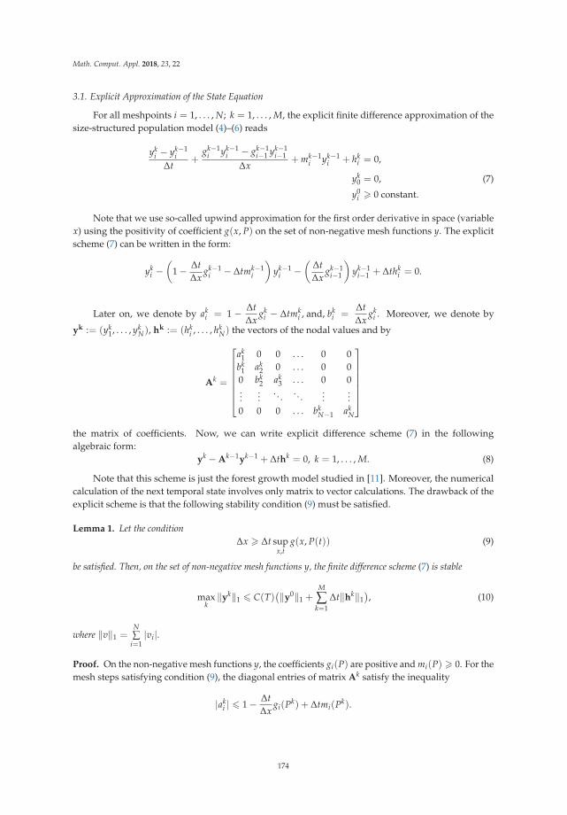
Math. Comput. Appl. 2018, 23, 22
3.1. Explicit Approximation of the State Equation
For all meshpoints i = 1, . . . , N; k = 1, . . . , M, the explicit finite difference approximation of thesize-structured population model (4)–(6) reads
yki − yk−1
iΔt
+gk−1
i yk−1i − gk−1
i−1 yk−1i−1
Δx+ mk−1
i yk−1i + hk
i = 0,
yk0 = 0, (7)
y0i � 0 constant.
Note that we use so-called upwind approximation for the first order derivative in space (variablex) using the positivity of coefficient g(x, P) on the set of non-negative mesh functions y. The explicitscheme (7) can be written in the form:
yki −
(1 − Δt
Δxgk−1
i − Δtmk−1i
)yk−1
i −(
ΔtΔx
gk−1i−1
)yk−1
i−1 + Δthki = 0.
Later on, we denote by aki = 1 − Δt
Δxgk
i − Δtmki , and, bk
i =ΔtΔx
gki . Moreover, we denote by
yk := (yk1, . . . , yk
N), hk := (hki , . . . , hk
N) the vectors of the nodal values and by
Ak =
⎡⎢⎢⎢⎢⎢⎢⎣ak
1 0 0 . . . 0 0bk
1 ak2 0 . . . 0 0
0 bk2 ak
3 . . . 0 0...
.... . . . . .
......
0 0 0 . . . bkN−1 ak
N
⎤⎥⎥⎥⎥⎥⎥⎦the matrix of coefficients. Now, we can write explicit difference scheme (7) in the followingalgebraic form:
yk − Ak−1yk−1 + Δthk = 0, k = 1, . . . , M. (8)
Note that this scheme is just the forest growth model studied in [11]. Moreover, the numericalcalculation of the next temporal state involves only matrix to vector calculations. The drawback of theexplicit scheme is that the following stability condition (9) must be satisfied.
Lemma 1. Let the conditionΔx � Δt sup
x,tg(x, P(t)) (9)
be satisfied. Then, on the set of non-negative mesh functions y, the finite difference scheme (7) is stable
maxk
‖yk‖1 � C(T)(‖y0‖1 +
M
∑k=1
Δt‖hk‖1), (10)
where ‖v‖1 =N∑
i=1|vi|.
Proof. On the non-negative mesh functions y, the coefficients gi(P) are positive and mi(P) � 0. For themesh steps satisfying condition (9), the diagonal entries of matrix Ak satisfy the inequality
|aki | � 1 − Δt
Δxgi(Pk) + Δtmi(Pk).
174

Math. Comput. Appl. 2018, 23, 22
Because of this inequality, we have the following estimate for ‖.‖1-norm of matrices, connectedwith ‖.‖1-norm of vectors:
‖Ak‖1 =N
∑i=1
(|aki |+ |bk
i |) � 1 + CmΔt
with Cm = supx,t m(x, P(t)). Due to this estimate and condition (9), we obtain from Equation (8)the inequality
‖yk‖1 � (1 + CmΔt)‖yk−1‖1 + Δt‖hk‖1 for all k = 1, 2, . . . , M,
whence stability estimate (10) follows.
The condition (9) means that the length of the time step Δt and width of the size class Δx have tobe chosen so that a tree cannot grow over one size class during one time step Δt (compare with [16]).
3.2. Implicit Approximation of the State Equation
For all meshpoints i = 1, . . . , N; k = 1, . . . , M, the implicit finite difference approximation ofthe models (4)–(6) is the following linearized problem, with nonlinear coefficients calculated on theprevious time level:
yki − yk−1
iΔt
+gk−1
i yki − gk−1
i−1 yki−1
Δx+ mk−1
i yki + hk
i = 0,
yk0 = 0, (11)
y0i � 0 constant.
Equation (11) can be rewritten as(1 +
ΔtΔx
gk−1i + Δtmk−1
i
)yk
i −ΔtΔx
gk−1i−1 yk
i−1 − yk−1i + Δthk
i = 0,
for all i = 1, . . . , N, k = 1, . . . , M.
Using the notations aki = 1 +
ΔtΔx
gki + Δtmk
i and bki = − Δt
Δxgk
i , we rewrite Equation (11) in a formof linear algebraic equations
Bk−1yk − yk−1 + Δthk = 0, k = 1, . . . , M, (12)
where
Bk :=
⎡⎢⎢⎢⎢⎢⎢⎣ak
1 0 0 . . . 0 0bk
1 ak2 0 . . . 0 0
0 bk2 ak
3 . . . 0 0...
.... . . . . .
......
0 0 0 . . . bkN−1 ak
N
⎤⎥⎥⎥⎥⎥⎥⎦is a matrix of nonlinear coefficients.
Lemma 2. Finite difference scheme (11) is unconditionally stable on the set of non-negative mesh functions y:for any Δt and Δx the following stability estimate holds:
maxk
‖yk‖1 � ‖y0‖1 +M
∑k=1
Δt‖hk‖1. (13)
175

Math. Comput. Appl. 2018, 23, 22
Proof. By direct calculations, we obtain from Equation (12) the equality
N
∑i=1
aki yk
i +N−1
∑i=1
bki yk
i −N
∑i=1
yk−1i + Δt
N
∑i=1
hki = 0.
Since aki + bk
i � 1 and akN � 1, then, from this equality, we get
N
∑i=1
yki �
N
∑i=1
yk−1i + Δt
N
∑i=1
|hki |.
Because of positivity of vectors yk and yk−1, the last inequality can be written in the form
‖yk‖1 � ‖yk−1‖1 + Δt‖hk‖1 ∀k,
whence stability estimate (13) follows.
Notice, contrary to the explicit scheme the time step Δt and class width Δx has no mutualdependence, hence the growth of a tree during a time step is not restricted less than one size class.This characteristic of the implicit scheme is useful in the optimal harvesting problem, covered by themodels (4)–(6) or parameter identification problem because such problems require solving the modelmany times before an optimal solution is obtained.
3.3. Approximation of the Optimal Control Problem
We denote dki := d(xi, tk) the discounted price for size class (xi−1, xi] at time tk, and dk = (dk
1, . . . , dkN).
Moreover, (u, v) := ∑N1 uivi is the vector product of vectors u, v ∈ R
N. Approximating the cost function (1)by the right-hand Riemann sum, we get the following approximation for the harvesting problem:
max(y,h)∈K
{J(y, h) :=
M
∑k=1
(dk, hk) =M
∑k=1
N
∑i=1
dki hk
i
}. (14)
Above, we denote by K = Yad × Had, where
Yad ={(y, h) |y � 0, y is a solution for Equations (7) or (11)}, (15)
Had ={h | 0 � hk � hmax, ‖hk‖1 � B or hk = 0, k = 1, . . . , M}. (16)
Moreover, y = (y1, . . . , yM) and h = (h1, . . . , hM).The following propositions show that the discrete optimal harvesting problem (14) has at least
one solution in both cases, i.e., if models (4)–(6) is approximated explicitly or implicitly.
Proposition 1. Let the mesh steps Δt and Δx satisfy the inequality
1 − ΔtΔx
supx,t
g(x, P(t))− Δt supx,t
m(x, P(t)) � 0. (17)
Then, Problem (14) has at least one solution if y satisfies Equation (7).
Proof. The set K is non-empty. In fact, due to assumption (17), the solution y of finite differencescheme (7) with y0 � 0 is non-negative if h = 0. This statement can be easily verified using form (8) ofthe difference scheme and noting that all entries ak
i and bki of the matrices Ak are non-negative.
Obviously, assumption (9) follows from inequality (17), so stability estimate (10) holds. Sincevector h ∈ K is bounded, then, due to inequality (10), there exists a constant Y such that ‖y‖1 � Y, i.e.,the set K is bounded. It is closed because of the continuity of functions g(P) and m(P) with respect
176

Math. Comput. Appl. 2018, 23, 22
to P, while P is obviously continuous with respect to y. Thus, K is compact. At last, cost functionJ of Problem (14) is continuous, whence the existence of a solution to Problem (14) follows fromWeierstrass’s theorem.
Proposition 2. Problem (14) has at least one solution if y satisfies Equation (11).
Proof. Proof is very similar to the proof of Proposition 1. Namely, the set K is non-empty because,for h = 0, the solution y of finite difference scheme (11) is non-negative for all Δx and Δt. Since h isbounded, then, due to stability estimate (13), y is also bounded, so the set K is bounded. It is closedbecause of the continuity of functions g(P) and m(P) with respect to P, and continuity of P withrespect to y. Thus, K is compact. At last, cost function J of Problem (14) is continuous, whence theexistence of a solution to Problem (14) follows.
Remark 1. Since neither the function J is strictly concave nor the set K is strictly convex, the optimizationproblem can have a non-unique solution.
4. Realization of the Optimal Strategies
In this section, a first order method to approximate the optimal harvesting problem (14) isconstructed. In real-life applications, the growth rate g and mortality rate m are determined ona statistical basis and the compatibility conditions required for high-order methods can be hardlyvalidated. Hence, a first order method, which is desirable to have a robust scheme but requiresminimum regularity of the solution should be the most adequate. The first order methods requirecomputing of the Fréchet derivatives (Jacobian matrix), which can be computationally expensive.However, when we consider the nonlinear optimization problem, only the gradient of the objectfunction is needed, and the gradient can be computed without the Fréchet derivatives. In this work,the adjoint approach developed in the 1970s in [17] is applied for calculation of the functional gradient.The adjoint method has a great advantage against the direct method because only one linear stateproblem, so called adjoint state, need to be solved for obtaining the gradient information. Today, it isa well-known method for computing the gradient of a functional with respect to model parameterswhen this functional depends on those model parameters trough state variables, which are solutionsof the state problem. However, this method is less well understood in the control of populationmodels, and, as far as we know, no applications to distributed optimal control of harvesting ispresented in literature. Duality and adjoint equations are essential tools in studying existence ofthe optimal pair (y, h), and, for a periodic age-dependent harvesting problem and for age-spatialstructured harvesting problem, it is applied for proving the existence of the bang-bang control in [18]and in [19,20], respectively. For continuous size-structured harvesting, problem duality and adjointequations are applied for proving the existence of the bang-bang control in [6,8].
In this work, we apply the Lagrange method and give a recipe to systematically define theadjoint state equations and gradient information. We formulate the Lagrangian of the problem (14)with respect to the state constraint (15) only, and use the projection method regarding the controlconstraint (16). In the projection method, if solution goes outside the constraint set (16), it is projectedback to there. Let us generalize and denote by A(y, h) = 0 the operator Equation (8) (or Equation (12)).Moreover, Ak(y, h) = 0 is the operator equation at the time level k, k = 1, . . . , M.
Suppose the functional J and operator A to be differentiable in the sense that there exist thefollowing partial derivatives:
Jyδy = limt→0
J(y + tδy, h)− J(y, h)
t, Jhδh = lim
t→0
J(y, h + tδh)− J(y, h)
t,
Ayδy = limt→0
A(y + tδy, h)− A(y, h)
t, Ahδh = lim
t→0
A(y, h + tδh)− A(y, h)
t
177

Math. Comput. Appl. 2018, 23, 22
for all vectors δy and δh (or at least for the vectors such that y, y + δy ∈ Yad and h, h + δh ∈ Had).Note that for the fixed h and y, Jy ≡ Jy(y, h) and Jh ≡ Jh(y, h) are vectors while Ay = Ay(y, h) andAh = Ah(y, h) are matrices. By A∗
y and A∗h, we denote the corresponding transpose matrices.
Let us define Lagrange function, L, of the problem (14) by
L(y, h, λ) = J(y(h), h)−M
∑k=1
(λk, Ak(y, h)),
where λk ∈ RN . Now, for all feasible pair (y, h) holds A(y, h) = 0, and, for any λ, we have:
L(y, h, λ) = J(y(h), h),
and, since λ does not depend on h, we have
∂ J∂h
=∂L(y, h, λ)
∂y
∂y
∂h+
∂L(y, h, λ)
∂h. (18)
Above, one method to approximate∂y
∂his to compute N finite differences over control variable h.
However, each computation requires solving the equation A(y, h) = 0, and, for large N, this method
is computationally expensive. In the adjoint method, we can avoid to compute∂y
∂hby solving the linear
adjoint state equation only once.The theory of constrained optimization, see [21], says that (y, h) is the optimal pair for the
problem (14) if (y, h, λ) is a saddle point of L. The derivatives of L with respect to y, h and λ are:
∂L(y, h, λ)
∂y=
∂ J(y, h)
∂y−(∂A(y, h)
∂y
)∗λ,
∂L(y, h, λ)
∂h=
∂ J(y, h)
∂h−(∂A(y, h)
∂h
)∗λ,
∂L(y, h, λ)
∂λ= −A(y, h).
Now,∂L(y, h, λ)
∂λ= 0 gives the state equation,
∂L(y, h, λ)
∂y= 0 gives the adjoint state equation
and∂ J∂h
=∂L(y, h, λ)
∂hgives the gradient.
Now, the calculation of the gradient can be summarized by the following steps when theLagrangian L(y, h, λ) = J(y, h)− (λ, A(y, h)) is first formulated:
I Solve the state equation A(y, h) = 0;II Solve the adjoint state equation
∂L(y, h, λ)
∂y=
∂ J(y, h)
∂y−(∂A(y, h)
∂y
)∗λ = 0;
III Compute the gradient
∂ J∂h
=∂ J(y, h)
∂h−(∂A(y, h)
∂h
)∗λ.
Partial derivatives of J(y, h) and A(y, h) are presented in Appendix A. Gradient∂ J∂h
we usedin projected gradient method [22], which we applied for iteration of a solution of the optimalharvesting problem.
178

Math. Comput. Appl. 2018, 23, 22
5. Numerical Example
In this section, we study numerical examples of problem (14). We compared two cases where thestate constraint (4) was approximated with explicit approximation (7) and implicit approximation (11).
As the discounted price for size class (xi−1, xi] at time tk, we used dki =
cpvpi + csvs
i
(1 + r)tk , where r is
the interest rate, cp and cs are the prices of the pulpwood and sawlog, respectively, and vpi and
vsi are the volumes of pulpwood and sawlog of a tree in size class (xi−1, xi], respectively. In the
optimizations, we used the following values for parameters: price of pulpwood cp = 16.56 em−3 andsawlog cs = 58.44 em−3, interest rate r = 3% and lower bound for harvested trees B = 50 m3 ha−1.The pulpwood and sawlog volumes vp
i and vsi we got from [10]. The optimization results of problem (14)
are presented in Tables 1 and 2, and in Figures 1 and 2.
Figure 1. Diameter distributions associated with optimal thinnings of problem (14) with state equationapproximated by explicit scheme (7). Numbers (e.g., 5–8, 11–14) represent diameter in centimetres.
179
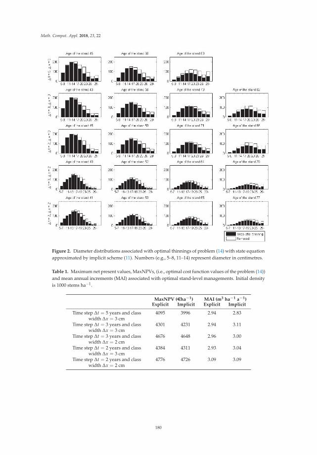
Math. Comput. Appl. 2018, 23, 22
Figure 2. Diameter distributions associated with optimal thinnings of problem (14) with state equationapproximated by implicit scheme (11). Numbers (e.g., 5–8, 11–14) represent diameter in centimetres.
Table 1. Maximum net present values, MaxNPVs, (i.e., optimal cost function values of the problem (14))and mean annual increments (MAI) associated with optimal stand-level managements. Initial densityis 1000 stems ha−1.
MaxNPV (eha−1) MAI (m3 ha−1 a−1)Explicit Implicit Explicit Implicit
Time step Δt = 5 years and classwidth Δx = 3 cm
4095 3996 2.94 2.83
Time step Δt = 3 years and classwidth Δx = 3 cm
4301 4231 2.94 3.11
Time step Δt = 3 years and classwidth Δx = 2 cm
4676 4648 2.96 3.00
Time step Δt = 2 years and classwidth Δx = 3 cm
4384 4311 2.93 3.04
Time step Δt = 2 years and classwidth Δx = 2 cm
4776 4726 3.09 3.09
180

Math. Comput. Appl. 2018, 23, 22
Table 2. Optimal stand-level managements generated by explicit (7) and implicit (11) approximationof the forest growth model (4). Initial density is 1000 stems ha−1.
Stand Age (a)Removal(m3 ha−1)
Thinning Intensity (% ofBasal Area Removed)
Saw LogProportion (%)
Explicit Implicit Explicit Implicit Explicit Implicit Explicit Implicit
Time step Δt = 5 years and class width Δx = 3 cm1st thinning 55 45 91.0 77.2 48 48 87 852nd thinning 70 60 68.9 59.3 46 46 88 873rd thinning 85 80 98.6 90.6 79 72 87 86final thinning 105 105 50.0 69.9 100 100 90 86total 308.5 297.0 88 86
Time step Δt = 3 years and class width Δx = 3 cm1st thinning 49 43 78.9 52.4 48 35 83 862nd thinning 64 58 68.2 54.3 50 35 86 893rd thinning 76 70 55.4 50.0 56 35 87 914th thinning - 82 - 72.4 - 59 - 86final thinning 100 100 91.5 82.2 100 100 88 85total 293.9 311.3 86 87
Time step Δt = 3 years and class width Δx = 2 cm1st thinning 46 40 60.6 60.5 36 40 83 812nd thinning 58 52 56.5 51.8 38 40 85 833rd thinning 70 64 59.7 52.1 45 46 88 864th thinning 79 79 50.0 55.0 52 56 89 90final thinning 94 97 72.6 71.4 100 100 89 86total 299.5 290.7 87 85
Time step Δt = 2 years and class width Δx = 3 cm1st thinning 47 45 62.2 59.1 39 38 84 862nd thinning 61 59 59.9 54.8 41 37 87 883rd thinning 75 71 58.9 50.0 44 37 90 904th thinning 83 85 64.4 78.0 70 64 84 87final thinning 101 103 50.0 71.0 100 100 86 86total 295.5 313.3 86 87
Time step Δt = 2 years and class width Δx = 2 cm1st thinning 43 41 55.3 58.5 36 38 80 822nd thinning 55 53 55.6 53.3 39 39 84 843rd thinning 65 65 50.0 52.0 42 44 86 874th thinning 77 77 53.0 50.2 53 51 89 89final thinning 95 95 79.5 79.2 100 100 89 87total 293.4 293.1 86 86
The results show that the maximum net present value (NPV) associated with the explicitapproximation (7) was higher than the corresponding of the implicit approximation (Table 1).When class width or time step decreased, maximum NPV increased in both cases. The difference ofmaximum NPVs between the two cases decreased when class width or time step decreased. Only whentime step decreased from three to two years, the difference of maximum NPVs increased. The differencewas biggest (99 e) when time step Δt = 5 years and class width Δx = 3 cm and smallest (28 e) whentime step Δt = 3 years and class width Δx = 2 cm.
With both approximations, three or four intermediate thinnings were made (Table 2). Numberof thinnings increased when time step and class width decreased. When implicit approximation (11)was used, first thinnings were made 1–2 time steps earlier, while the last few thinnings were made0–2 time steps later than when explicit approximation (7) was used. The thinning intensities werealmost identical between the two approximations. If there was some difference, intensity was usuallybigger when explicit approximation (7) was used (Table 2). The thinning pattern was in all optimalmanagements quite similar: in each thinning, more big trees than small ones were removed indicatinga thinning from-above method (for different thinning types, see e.g., [23], pp. 727, 733). Thinning from
181

Math. Comput. Appl. 2018, 23, 22
above has proven to be the best thinning type in stand-level optimizations of even-aged boreal forests(e.g., [24]). When explicit approximation (7) was used, all trees from two or three of the biggest sizeclasses were removed (Figure 1). On the other hand, when implicit approximation (11) was applied,only part of the trees from those size classes were removed (Figure 2).
6. Discussion
This study contributes to existing literature on forest management by providing a theoreticallysound framework to solve nonlinear optimization problem of even-aged stands. We compared theresults of forest management optimizations, when the explicit and implicit approximations of the forestgrowth model was used. The optimization results show that the differences of the results betweenapproximations are diminutive. This was expected as solutions of both approximation equations areproved to converge to solutions of continuous equation [5,14].
In numerical examples, we used data from the Scots pine (Pinus sylvestris L.) stands that werelocated in Northern Ostrobothnia, Finland, on nutrient-poor soil type. The data was the same asin [11]. The difference is that, in [11], data was fitted directly to the matrix model, as, in this study,we first fitted data to the continuous model and then approximated it with a matrix model. In [11],the time step was five years and class width 3 cm. The results are in line with each other. Both methodsgave four thinnings in optimal management and thinning from above dominated as the thinningtype. In [11], the optimal net present value was slightly higher and, in the optimal management,the thinnings were made slightly earlier than in this study.
The optimal harvesting problem with a continuous size-structured population model was studiedin [6–8]. In those papers, harvesting was defined as a proportion of removed trees. The maximumprinciple for the problem was proved in [6,8]. Moreover, in [7], the strong bang-bang principle undersome additional (but realistic) conditions was proved. This means that the optimal solution has thestructure, where all trees bigger than some certain size are removed. In our results, the solution ofthe optimization problem, where state constraint was approximated with explicit approximation,was nearer that structure. In addition, the optimization results were a little better then. However,when explicit approximation is used, the time step and class width have to be chosen so thata tree cannot grow over one size class during one time step [16]. We proved that only then is theexplicit approximation scheme stable. For the implicit approximation scheme, we proved that it isunconditionally stable. Thus, in implicit approximation, the time step and class width can be chosenfreely. In general, explicit approximation of the population model is more commonly used as a forestgrowth model [9,16].
Author Contributions: J.P. made the approximations and conducted the optimizations under supervision of E.L.;A.L. proved the theoretical results; J.P. and A.A. analyzed the numerical results; all authors contributed to thewriting of the manuscript.
Acknowledgments: We want to acknowledge the Jenny and Antti Wihuri foundation for financial support.
Conflicts of Interest: The authors declare no conflict of interest.
Appendix A
We used the adjoint method to solve the optimization problem (14). For that, we needed thepartial derivatives of the Lagrangian
L(y, h, λ) = J(y, h)−M
∑k=1
(λk, Ak(y, h)),
where J(h) = ∑Mk=1(d
k, hk) is cost function of problem (14) and Ak(y, h) is constraint (8) or (12).First, we calculate the partial derivatives of the cost function J(y, h). Since it depends only on h,
obviously∂ J∂y
= 0. The partial derivative of the cost function J with respect to h is
182
Math. Comput. Appl. 2018, 23, 22
∂ J(h)∂h
= d.
Next, we calculate the partial derivatives of constraint function A(y, h). In both forms of A
(constraints (8) or (12)), the partial derivative with respect to h is∂A(y, h)
∂h= Δt.
Let us calculate the partial derivative of constraint function (8) (explicit approximation of the stateEquation (4)) with respect to y
∂(λ, A(y, h))
∂y=
∂
∂y
M
∑k=1
(λk, yk − Ak−1yk−1 + Δthk). (A1)
Let us denote
Hk := Akyk =
⎡⎢⎢⎢⎢⎣ak
1yk1
ak2yk
2 + bk1yk
1...
akNyk
N + bkN−1yk
N−1
⎤⎥⎥⎥⎥⎦ .
Then, the partial derivative (A1) can be written in the form
∂(λ, A(y, h))
∂y=
∂
∂y
(M
∑k=1
(λk, yk − Hk−1)
).
By rearranging the terms and defining λM+1 = 0, we get
∂(λ, A(y, h))
∂y=
∂
∂y
((λ1, H0) +
M
∑k=1
((λk, yk)− (λk+1, Hk))
).
Now,∂H0
∂y= 0 by definition of y0 and
∂Hk
∂y= Ak + Hk
1, k = 1, . . . , M − 1, where
Hk1 =
⎡⎢⎢⎢⎢⎣ak
11yk1 . . . ak
1Nyk1
ak21yk
2 + bk11yk+1
1 . . . ak2Nyk
2 + bk1Nyk
1...
. . ....
akN1yk
N + bkN−1,1yk
N−1 . . . akNNyk
N + bkN−1,Nyk
N−1
⎤⎥⎥⎥⎥⎦ ,
and
akij =
∂aki
∂ykj= − Δt
Δx(g21 + g22xi)
( xj
2
)2π − Δt
(m21 +
m22
xi+
m23
x2i
)( xj
2
)2π, (A2)
bkij =
∂bki
∂ykj=
ΔtΔx
(g21 + g22xi)
( xj
2
)2π. (A3)
Thus, we can define
∂(λ, A(y, h))
∂y= (w1, w2, . . . , wM),
where
wk = λk − ((Ak)∗ + (Hk1)
∗)λk+1, k = 1, . . . , M − 1
wM = λM.
183

Math. Comput. Appl. 2018, 23, 22
Then, we calculate the partial derivative of constraint (12) (implicit approximation of the stateEquation (4)) with respect to y
∂(λ, A(y, h))
∂y=
∂
∂y
M
∑k=1
(λk, Bk−1yk − yk−1 + Δthk). (A4)
Let us denote
Gk = Bk−1yk =
⎡⎢⎢⎢⎢⎣ak−1
1 yk1
ak−12 yk
2 − bk−11 yk
1...
ak−1N yk
N − bk−1N−1yk
N−1
⎤⎥⎥⎥⎥⎦ .
Then, the partial derivative (A4) can be written in the form
∂(λ, A(y, h))
∂y=
∂
∂y
M
∑k=1
(λk, Gk − yk−1).
Note that function Gk depends on yk−1 and yk so the partial derivative∂Gk
∂y=
∂Gk
∂yk−1 +∂Gk
∂yk .
By definition of y0, derivative∂(λ1, y0)
∂y= 0 and derivative
∂(λ1, G1)
∂y=
∂(λ1, G1)
∂y1 . By rearranging
the terms and defining λM+1 = 0, we get
∂(λ, A(y, h))
∂y=
M
∑k=1
(∂(λk, Gk)
∂yk +∂(λk+1, Gk+1 − yk)
∂yk
).
Derivative∂Gk
∂yk = Bk−1 and derivative
∂Gk+1
∂yk =
⎡⎢⎢⎢⎢⎣ak
11yk+11 . . . ak
1Nyk+11
ak21yk+1
2 − bk11yk+1
1 . . . ak2Nyk+1
2 − bk1Nyk+1
1...
. . ....
akN1yk+1
N − bkN−1,1yk+1
N−1 . . . akNNyk+1
N − bkN−1,Nyk+1
N−1
⎤⎥⎥⎥⎥⎦ ,
where akij and bk
ij are derivatives of coefficients aki and bk
i with respect to ykj defined in
Equations (A2) and (A3), respectively. Thus, we can define
∂(λ, A(y, h))
∂y= (q1, q2, . . . , qM),
where
qk = (Bk−1)∗λk +
((∂Gk+1
∂yk
)∗− 1N
)λk+1, k = 1, . . . , M − 1,
qM = (BM−1)∗λM,
and 1N is N × N identity matrix.
References
1. Kato, N.; Torikata, H. Local existence for a general model of size-dependent population dynamics.Abstr. Appl. Anal. 1997, 2, 207–226. [CrossRef]
184

Math. Comput. Appl. 2018, 23, 22
2. Kato, N. A general model of size-dependent population dynamics with nonlinear growth rate. J. Math.Anal. Appl. 2004, 297, 234–256. [CrossRef]
3. Calsina, A.; Saldana, J. A model of physiologically structured population dynamics with a nonlinearindividual growth rate. J. Math. Biol. 1995, 33, 335–364. [CrossRef]
4. Calsina, A.; Saldana, J. Basic theory for a class of models of hierarchically structured population dynamicswith distributed states in the recruitment. Math. Model. Meth. Appl. Sci. 2006, 16, 16951722. [CrossRef]
5. Ackleh, A.S.; Deng, K.; Hu, S.A. Quasilinear Hierarchical Size-Structured Model: Well-Posedness andApproximation. Appl. Math. Optim. 2005, 51, 3559. [CrossRef]
6. Hritonenko, N.; Yatsenko, Y.; Goetz, R.-U.; Xabadia, A. Maximum principle for size-structured model of forestand carbon sequestration management. Appl. Math. Lett. 2008, 21, 1090–1094 [CrossRef]
7. Hritonenko, N.; Yatsenko, Y.; Goetz, R.-U.; Xabadia, A. A bang-bang regime in optimal harvesting ofsize-structured populations. Nonlinear Anal. Theory Methods Appl. 2009, 71, e2331–e2336. [CrossRef]
8. Hritonenko, N.; Yatsenko, Y.; Goetz, R.-U.; Xabadia, A. Optimal harvesting in forestry: Steady-state analysisand climate change impact. J. Biol. Dyn. 2013, 7, 41–58. [CrossRef] [PubMed]
9. Liang, J.; Picard, N. Matrix model of Forest Dynamics: An Overview and Outlook. For. Sci. 2013, 59, 359–378.[CrossRef]
10. Rämö, J.; Tahvonen, O. Economics of harvesting uneven-aged forest stands in Fennoscandia. Scand. J. For. Res.2014, 29, 777–792. [CrossRef]
11. Pyy, J.; Ahtikoski, A.; Laitinen, E.; Siipilehto, J. Introducing a non-stationary matrix model for stand-leveloptimization, an even aged Pine (Pinus sylvestris L.) stand in Finland. Forests 2017, 8, 163. [CrossRef]
12. Anita, S.; Ianneli, M.; Kim, M.-Y.; Park, E.-J. Optimal harvesting for periodic age-dependent populationdynamics. SIAM J. Appl. Math. 1998, 58, 1648–1666.
13. Xie, Q.; He, Z.-R.; Wang, X. Optimal harvesting in diffusive population models with size random growth anddistributed recruitment. Electron. J. Differ. Eq. 2016, 214, 1–13.
14. Ackleh, A.S.; Farkas, J.Z.; Li, X.; Ma, B. Finite difference approximations for a size-structured populationmodel with distributed states in the recruitment. J. Biol. Dyn. 2015, 9, 2–31. [CrossRef] [PubMed]
15. Ackleh, A.S.; Ito, K. An implicit finite difference scheme for the nonlinear size-structured population model.Numer. Func. Anal. Opt. 1997, 18, 865–884. [CrossRef]
16. Picard, N.; Liang, J. Matrix models for size structured populations: Unrealistic fast growth or simply diffusion?PLoS ONE 2014, 9, e98254. [CrossRef] [PubMed]
17. Lions, J. Nonhomogeneous Boundary Value Problems and Applications; Springer Verlag: Berlin, German, 1972.18. Anita, S.; Arnautu, V.; Stefanescu, R. Numerical optimal harvesting for periodic age-structured population
dynamics with logistic term. Numer. Func. Anal. Opt. 2009, 30, 183–198. [CrossRef]19. Kang, Y.H.; Lee, M.J.; Jung, I.H. Optimal Harvesting for an Age-Spatial-Structured Population Dynamic
Model with External Mortality. Abstr. Appl. Anal. 2012. [CrossRef]20. Kim, Y.K.; Lee, M.J.; Jung, I.H. Duality in an Optimal Harvesting Problem by a Nonlinear Age-Spatial
Structured Population Dynamic System. KYUNGPOOK Math. J. 2011, 51, 353–364. [CrossRef]21. Ciarlet, P.G. Introduction to Numerical Linear Algebra and Optimization; Cambridge University Press: New York,
United States, 1989.22. Anita, S.; Arnautu, V.; Capasso, V. An Introduction to Optimal Control Problems in Life Sciences and Economics:
From Mathematical Models to Numerical Simulation with MATLAB; Springer: Dordrecht, The Netherlands, 2011.23. Kuuluvainen, T.; Tahvonen, O.; Aakala, T. Even-aged and uneven-aged forest management in boreal
Fennoscandia: A review. AMBIO 2012, 41, 720–737. [CrossRef] [PubMed]24. Tahvonen, O.; Pihlainen, S.; Niinimäki, S. On the economics of optimal timber production in boreal Scots pine
stand. Can. J. For. Res. 2013, 43, 719–730. [CrossRef]
c© 2018 by the authors. Licensee MDPI, Basel, Switzerland. This article is an open accessarticle distributed under the terms and conditions of the Creative Commons Attribution(CC BY) license (http://creativecommons.org/licenses/by/4.0/).
185

Article
Solution of Fuzzy Differential Equations Using FuzzySumudu Transforms
Raheleh Jafari 1,* ID and Sina Razvarz 2 ID
1 Department of Information and Communication Technology, University of Agder, 4879 Grimstad, Norway2 Departamento de Control Automático, CINVESTAV-IPN (National Polytechnic Institute),
07360 Mexico City, Mexico; [email protected]* Correspondence: [email protected]; Tel.: +47-3723-3000
Received: 15 December 2017; Accepted: 16 January 2018; Published: 17 January 2018
Abstract: The uncertain nonlinear systems can be modeled with fuzzy differential equations (FDEs)and the solutions of these equations are applied to analyze many engineering problems. However,it is very difficult to obtain solutions of FDEs. In this paper, the solutions of FDEs are approximatedby utilizing the fuzzy Sumudu transform (FST) method. Significant theorems are suggested in orderto explain the properties of FST. The proposed method is validated with three real examples.
Keywords: uncertain nonlinear system; modeling; fuzzy Sumudu transform
1. Introduction
In many physical and dynamical processes, mathematical modeling leads to the deterministicinitial and boundary value problems. In practice, the boundary values may be different from crisp anddisplays in the form of unknown parameters [1]. The qualitative behavior of solutions of the equationsis associated with the errors. If the errors are random, in this case, we have a stochastic differentialequation along with the random boundary value. Moreover, if the errors are not probabilistic, the fuzzynumbers are substituted by random variables [1,2]. The fuzzy derivative, as well as fuzzy differentialequations (FDE), have been discussed in [3,4]. The Peano-like theorems for FDEs, and system ofFDE on R (Real line) is investigated in [5]. The first-order fuzzy initial value problem, and the fuzzypartial differential equation, have been studied in [5]. The simulation of the fuzzy system is discussedin [6–11]. The application of numerical techniques for resolving FDEs has been illustrated in [12].The Lipschitz condition and the theorem for existence and uniqueness of the solution related to FDEs,are discussed in [13–15]. The fractional fuzzy Laplace transformation has been mentioned in [13].
An advanced method to solve FDEs is laid down based on the Sumudu transform.Sumudu transform along with broad applications has been utilized in the area of system engineeringand applied physics. Recently, Sumudu transform is popularized in order to solve fractional localdifferential equations [16–20]. In [21], Sumudu transform is suggested in order to solve fuzzy partialdifferential equations. Some fundamental theorems along with some properties for Sumudu transformare mentioned in [22]. In [23] the variational iteration technique is proposed utilizing Sumudutransform for solving ordinary equations.
In this paper, we use FST to approximate the solutions of the FDEs. We extend our previouswork [24] by generating more theorems for describing the properties of FST. Moreover, the comparisonbetween our method with other numerical methods has been carried out. The FST reduces the FDE toan algebraic equation. A very important property of the FST is that it can solve the equation withoutresorting to a new frequency domain. By utilizing the proposed technique, the fuzzy boundary valueproblem can be resolved directly without determining a general solution.
This paper is organized as follows: in Section 2 some definitions which have been used in thispaper are given. Section 3 demonstrates the properties of FST. In Section 4 solving FDEs by utilizing
Math. Comput. Appl. 2018, 23, 5; doi:10.3390/mca23010005 www.mdpi.com/journal/mca186

Math. Comput. Appl. 2018, 23, 5
FST approach is described. Three real examples are used to demonstrate the efficiency of the proposedmethod in Section 5. Section 6 provides the conclusion to the paper.
2. Preliminaries
Some concepts related to the fuzzy calculations are laid down in this section [25,26].
Definition 1. A fuzzy number B is a function of B ∈ E : R → [0, 1], in such a manner, (1) B is normal,(there exists a0 ∈ R in such a manner B(a0) = 1); (2) B is convex, B(γa + (1 − γ)c) ≥min{B(a), B(c)},∀a, c ∈ R, ∀γ ∈ [0, 1]; (3) B is upper semi-continuous on R, i.e., B(a) ≤ B(a0) + ε, ∀a ∈ N(a0), ∀a0 ∈ R,∀ε > 0, N(a0) is a neighborhood; (4) The set B+ = {a ∈ R, B(a) > 0} is compact.
Definition 2. The r-level of the fuzzy number B is defined as follows
[B]r = {a ∈ R : B(a) ≥ r} (1)
where 0 < r ≤ 1, B ∈ E.
Definition 3. Let B1, B2 ∈ E and ξ ∈ R, the operations addition, subtraction, multiplication and scalarmultiplication are defined as
[B1 ⊕ B2]r = [B1]
r + [B2]r = [Br
1 + Br2, Br
1 + Br2] (2)
[B1 � B2]r = [B1]
r − [B2]r = [Br
1 − Br2, Br
1 − Br2] (3)
[B1 � B2]r =
(min{Br
1Br2, Br
1Br2, Br
1Br2, Br
1Br2}
max{Br1Br
2, Br1Br
2, Br1Br
2, Br1Br
2}
)(4)
[ξB1]r = ξ[B1]
r =
{(ξBr
1, ξBr1), ξ ≥ 0
(ξBr1, ξBr
1), ξ ≤ 0(5)
Definition 4. The Hausdroff distance between two fuzzy numbers B1 and B2 is defined as [27,28]
D(B1, B2) = sup0≤r≤1
{max(|Br1 − Br
2|, |Br1 − Br
2|)} (6)
D(B1, B2) has the following properties
(i) D(B1 ⊕ u, B2 ⊕ u) = D(B1, B2), ∀B1, B2, u ∈ E(ii) D(ξB1, ξB2) =| ξ | D(B1, B2), ∀ξ ∈ R, B1, B2 ∈ E(iii) D(B1 ⊕ B2, u ⊕ v) ≤ D(B1, u) + D(B2, v), ∀B1, B2, u, v ∈ E(iv) (D, E) is stated as complete metric space.
Definition 5. The function ψ : [a1, a2] −→ E is integrable on [a1, a2], if it satisfies in the belowmentioned relation ∫ ∞
a1
ψ(x)dx = (∫ ∞
a1
ψ(x, r)dx,∫ ∞
a1
ψ(x, r)dx) (7)
If ψ(x) be a fuzzy value function, as well as q(x) be a fuzzy Riemann integrable on [a1, ∞] so ψ(x)⊕ q(x)can be a fuzzy Riemann integrable on [a1, ∞]. Therefore,∫ ∞
a1
(ψ(x)⊕ q(x))dx =∫ ∞
aψ(x)dx ⊕
∫ ∞
aq(x)dx (8)
According to fuzzy concept or in the case of interval arithmetic, equation B1 = B2 ⊕ s is not equivalentwith s = B1 � B2 = B1 ⊕ (−1)B2 or to B2 = B1 � s = B1 ⊕ (−1)s and this is the main reason in introducingthe following Hukuhara difference (H-difference).
187

Math. Comput. Appl. 2018, 23, 5
Definition 6. The definition of H-difference [29,30], is proposed by B1 �H B2 = s ⇐⇒ B1 = B2 ⊕ s.If B1 �H B2 prevails, its r-level is [B1 �H B2]
r = [Br1 − Br
2, Br1 − Br
2]. Precisely, B1 �H B1 = 0 butB1 � B1 = 0.
Definition 7. Suppose ψ : [a1, a2] −→ E and x0 = [a1, a2]. ψ is strongly generalized differentiable at x0, if forall k > 0 adequately minute, ψ′(x0) ∈ E exists in such a manner that
(i) ∃ ψ(x0 + k)�H ψ(x0), ψ(x0)�H ψ(x0 − k) and
limk→0+ψ(x0+k)�Hψ(x0)
k = limk→0+ψ(x0)�Hψ(x0−k)
k = ψ′(x0)
(ii) ∃ ψ(x0)�H ψ(x0 + k), ψ(x0 − k)�H ψ(x0) and
limk→0+ψ(x0)�Hψ(x0+k)
(−k) = limk→0+ψ(x0−k)�Hψ(x0)
(−k) = ψ′(x0),
(iii) ∃ ψ(x0 + k)�H ψ(x0), ψ(x0 − k)�H ψ(x0) and
limk→0+ψ(x0+k)�Hψ(x0)
k = limk→0+ψ(x0−k)�Hψ(x0)
(−k) = ψ′(x0)
(iv) ∃ ψ(x0)�H ψ(x0 + k), ψ(x0)�H ψ(x0 − k) and
limk→0+ψ(x0)�Hψ(x0+k)
(−k) = limk→0+ψ(x0)�Hψ(x0−k)
k = ψ′(x0)
Remark 1. It is clear that case (i) is H-derivative. Furthermore, a function is (i)-differentiable only when it isH-derivative.
Remark 2. It can be concluded from [29] that, the definition of differentiability is non contradictory [31].
Let us consider ψ : R → E where ψ(t) has a parametric form as [ψ(t, r)] = [ψ(t, r), ψ(t, r)], for all0 ≤ r ≤ 1, thus [31]
(i) If ψ be (i)-differentiable, so ψ(t, r) and ψ(t, r) are differentiable functions, moreover ψ′(t) =
(ψ′(t, r), ψ′(t, r)).
(ii) If ψ be (ii)-differentiable, so ψ(t, r) and ψ(t, r) are differentiable functions, moreover ψ′(t) =
(ψ′(t, r), ψ′(t, r)).
Suppose f : (a1, a2) → R is differentiable on (a1, a2), furthermore ψ′ has finite root in (a1, a2),and m ∈ E, therefore, ψ(x) = m f (x) is strongly generalized differentiable on (a1, a2) along withψ′(x) = m f ′(x), ∀x ∈ (a1, a2).
Theorem 1. In [30] Assume ψ : R × E → E is taken to be a continuous fuzzy function. If x0 ∈ R, the fuzzyinitial value constraint {
φ′(t) = ψ(x, φ)
φ(x0) = φ0(9)
is incorporated with two solutions: (i)-differentiable, also (ii)-differentiable. Hence the successive iterations
φn+1(x) = φ0 +∫ x
x0
ψ(t, φn(t))dt, ∀x ∈ [x0, x1] (10)
andφn+1(x) = φ0 �H (−1)
∫ x
x0
ψ(t, φn(t))dt, ∀x ∈ [x0, x1] (11)
approaches towards the two solutions sequentially.
188

Math. Comput. Appl. 2018, 23, 5
Theorem 2. [29] The FDE is equivalent to a system of ordinary differential equations under generalizeddifferentiability.
3. Fuzzy Sumudu Transform
Fuzzy initial and boundary value problems can be resolved by utilizing fuzzy Laplacetransform [13]. In this paper, the FST methodology is illustrated; furthermore, the properties ofthis methodology are stated. By applying the FST methodology, the FDE is reduced to an algebraicequation. The main advantageous of the FST is that it can resolve the equation without resorting toa new frequency domain. The methodology of converting FDEs to an algebraic equation is expressedin [13].
Definition 8. Suppose ψ(t) be a continuous fuzzy value function, also, ψ(Bt)� e−t be an improper fuzzyRiemann integrable on [0, ∞). Accordingly,
∫ ∞0 ψ(Bt) � e−tdt is expressed as FST and it is defined by
Ω(B) = S[ψ(t)] =∫ ∞
0 ψ(Bt)� e−tdt, where 0 ≤ B < K, K ≥ 0, also e−t is real valued function. Based onthe Theorem 4 we have the following relation∫ ∞
0ψ(Bt)� e−tdt = (
∫ ∞
0ψ(Bt, r)e−tdt,
∫ ∞
0ψ(Bt, r)e−tdt) (12)
LetS[ψ(t, r)] =
∫ ∞0 ψ(Bt, r)e−tdt
S[ψ(t, r)] =∫ ∞
0 ψ(Bt, r)e−tdt(13)
hence we obtain the following relation
S[ψ(t)] = (S[ψ(t, r), Sψ(t, r)]) (14)
Theorem 3. Suppose ψ′(t) be a fuzzy value integrable function, as well as ψ(t) be the primitive of ψ′(t) on[0, ∞). Therefore,
S[ψ′(t)] = 1B� S[ψ(t)]� (
1B� [ψ(0)]) (15)
where ψ is considered to be (i)-differentiable, or
S[ψ′(t)] = −1B
� [ψ(0)]� (−1B
� S[ψ(t)]) (16)
where ψ is considered to be (ii)-differentiable.
Proof. For arbitrary fixed r ∈ [0, 1] we have
1B � S[ψ(t)]� ( 1
B � ψ(0))= ( 1
B S[ψ(t, r)]− 1B S[ψ(0, r)], 1
B S[ψ(t, r)]− 1B S[ψ(0, r)])
(17)
We have the following relations
S[ψ′(t, r)] = 1
B S[ψ(t, r)]− 1B [ψ(0, r)]
S[ψ′(t, r)] = 1B S[ψ(t, r)]− 1
B [ψ(0, r)](18)
Hence, we obtain
1B� S[ψ(t)]� (
1B� ψ(0)) = (S[ψ′(t, r)], S[ψ′
(t, r)]) (19)
189

Math. Comput. Appl. 2018, 23, 5
If ψ is cosidered to be (i)-differentiable, so
1B� S[ψ(t)]� (
1B� ψ(0)) = S[ψ′(t)] (20)
Let ψ is (ii)-differentiable. For arbitrary fixed α ∈ [0, 1] we obtain
−1B � [ψ(0)]� (−1
B � S[ψ(t)])= (−1
B ψ(0, r) + 1B S[ψ(t, r)], −1
B ψ(0, r) + 1B S[ψ(t, r)])
(21)
The above equation can be written as the following relation
−1B � [ψ(0)]� (−1
B � S[ψ(t)])= ( 1
B S[ψ(t, r)]− 1B ψ(0, r), 1
B S[ψ(t, r)]− 1B ψ(0, r))
(22)
We obtainS[ψ′
(t, r)] = 1B S[ψ(t, r)]− 1
B ψ(0, r)S[ψ′(t, r)] = 1
B S[ψ(t, r)]− 1B ψ(0, r)
(23)
So, we have
(−1B
ψ(0))� (−1B
� S[ψ(t)]) = (S[ψ′(t, r)], S[ψ′(t, r)]) (24)
Hence(−1B
ψ(0))� (−1B
� S[ψ(t)]) = S([ψ′(t, r)], [ψ′(t, r)]) (25)
Since ψ is (ii)-differentiable, therefore,
(−1B
ψ(0))� (−1B
� S[ψ(t)]) = S[ψ′(t)] (26)
Theorem 4. Taking into consideration that Sumudu transform is a linear transformation, so if ψ(t) and ϑ(t)be continuous fuzzy valued functions, moreover k1 as well as k2 be constant, therefore the following relation canbe obtained
S[(k1 � ψ(t))⊕ (k2 � ϑ(t))] = (k1 � S[ψ(t)])⊕ (k2 � S[ϑ(t)]) (27)
Proof. We have
S[(k1 � ψ(t))⊕ (k2 � ϑ(t))] =∫ ∞
0 (k1 � ϕ(Bt)⊕ k2 � ϑ(Bt))� e−tdt=∫ ∞
0 k1 � ψ(Bt)� e−tdt ⊕ ∫ ∞0 k2 � ϑ(Bt)� e−tdt
= k1 � (∫ ∞
0 ψ(Bt)� e−tdt)⊕ k2 � (∫ ∞
0 ϑ(Bt)� e−tdt)= k1 � S[ψ(t)]⊕ k2 � S[ϑ(t)]
(28)
Therefore, we conclude
S[(k1 � ψ(t))⊕ (k2 � ϑ(t))] = (k1 � S[ψ(t)])⊕ (k2 � S[ϑ(t)]) (29)
Lemma 1. Assume that the ψ(t) is a continuous fuzzy value function on [0, ∞), also γ ≥ 0, thus
S[γ � ψ(t)] = γ � S[ψ(t)] (30)
190

Math. Comput. Appl. 2018, 23, 5
Proof. Fuzzy Sumudu transform γ � ψ(t) is defined as
S[γ � ψ(t)] =∫ ∞
0γ � ψ(Bt)� e−tdt (31)
furthermore, we have ∫ ∞
0γ � ψ(Bt)� e−tdt = γ �
∫ ∞
0ψ(Bt)� e−tdt (32)
therefore,S[γ � ψ(t)] = γ � S[ψ(t)] (33)
Lemma 2. Assume that the ψ(t) is a continuous fuzzy value function, and ϑ(t) ≥ 0. Furthermore, if wesuppose that the (ψ(t)� ϑ(t))� e−t is improper fuzzy Reiman integrable on [0, ∞), then∫ ∞
0 (ψ(Bt)� ϑ(Bt))� e−tdt= (
∫ ∞0 ϑ(Bt)ψ(Bt, r)e−tdt,
∫ ∞0 ϑ(Bt)ψ(Bt, r)e−tdt)
(34)
Theorem 5. Suppose ψ(t) is a continuous fuzzy value function, also S[ψ(t)] = D(B), therefore,
S[ea1t � ψ(t)] =1
1 − a1BD(
B1 − a1B
) (35)
where ea1t is considered to be a real value function, also 1 − a1B > 0.
Proof. We have the following relation
S[ea1t � ψ(t)] =∫ ∞
0 ea1Bte−tψ(Bt)dt= (
∫ ∞0 e−(1−a1B)tψ(Bt, r)dt,
∫ ∞0 e−(1−a1B)tψ(Bt, r)dt)
(36)
Let us consider z = 1 − a1Bt, then
S[ea1t � ψ(t)] = 11−a1B (
∫ ∞0 ψ( Bz
1−a1B , r)e−zdz,∫ ∞
0 ψ( Bz1−a1B , r)e−zdz)
= { 11−a1B D( B
1−a1B ),1
1−a1B D( B1−a1B )} = 1
1−a1B D( B1−a1B )
(37)
4. Solving Fuzzy Initial Value Problem with Fuzzy Sumudu Transform Method
Consider the following fuzzy initial value problem{φ′(t) = ψ(t, φ(t)),
φ(0) = (φ(0, r), φ(0, r)), 0 < r ≤ 1(38)
where ψ(t, φ(t)) is a fuzzy function. The fuzzy function ψ(t, φ(t)) is the mapping of ψ : R × E → E.By utilizing FST method, we obtain
S[φ′(t)] = S[ψ(t, φ(t))] (39)
The resolving process of Equation (39) is based on the following cases.Case 1: Assume that the φ′(t) is (i)-differentiable. Based on the Theorem 4 we extract
φ′(t) = (φ′(t, r), φ′(t, r)) (40)
191
Math. Comput. Appl. 2018, 23, 5
S[φ′(t)] = (1B� S[φ(t)])� 1
Bφ(0) (41)
Equation (41) can be displayed as following relation{S[ψ(t, φ(t), r)] = 1
B S[φ(t, r)]− 1B φ(0, α)
S[ψ(t, φ(t), r)] = 1B S[φ(t, r)]− 1
B φ(0, r)(42)
where {ψ(t, φ(t), r) = min{ψ(t, B)|B ∈ (φ(t, r), φ(t, r))}ψ(t, φ(t), r) = max{ψ(t, B)|B ∈ (φ(t, r), φ(t, r))} (43)
Accordingly, Equation (43) can be resolved on the basis of the following assumptions
S[φ(t, r)] = U1(B, r) (44)
S[φ(t, r)] = U2(B, r) (45)
where U1(B, r), as well as U2(B, r) are the solutions of the Equation (43). By applying inverse Sumudutransform, φ(t, r) as well as φ(t, r) are computed as
φ(t, r) = S−1[U1(B, r)] (46)
φ(t, r) = S−1[U2(B, r)] (47)
Case 2: Assume that the φ′(t) is (ii)-differentiable. Based on the Theorem 4 we extract
φ′(t) = (φ′(t, r), φ′(t, r)) (48)
S[φ′(t)] = (−1B
� φ(0))� (−1B
� S[φ(t)]) (49)
Equation (49) can be displayed as following relation{S[ψ(t, φ(t), r)] = 1
B S[φ(t, r)]− 1B φ(0, r)
S[ψ(t, φ(t), r)] = 1B S[φ(t, r)]− 1
B φ(0, r)(50)
where {ψ(t, φ(t), r) = min{ψ(t, B)|B ∈ (φ(t, r), φ(t, r))}ψ(t, φ(t), r) = max{ψ(t, B)|B ∈ (φ(t, r), φ(t, r))} (51)
Accordingly, Equation (51) can be resolved on the basis of the following assumptions
S(φ(t, r) = V1(B, r)S(φ(t, r) = V2(B, r)
(52)
where V1(B, r), and V2(B, r) are the solutions of the Equation (51). By applying inverse Sumudutransform, φ(t, r) as well as φ(t, r) are computed as
φ(t, r) = S−1[V1(B, r)]φ(t, r) = S−1[V2(B, r)]
(53)
5. Examples
The following examples have been used to narrate the methodology proposed in this paper.
192

Math. Comput. Appl. 2018, 23, 5
Example 1. A tank with a heating system is displayed in Figure 1, where R = 0.5, the thermal capacitance isC = 2 also the temperature is ψ. The model is formulated as follows [13,32],{
φ′(t) = − 1RC
φ(t), 0 ≤ t ≤ Tφ(0) = (φ(0, r), φ(0, r))
(54)
By utilizing the FST method, we obtain
S[φ′(t)] = S[−φ(t)] (55)
S[φ′(t)] =∫ ∞
0φ′(Bt)� e−tdt (56)
where 0 ≤ B < K. If φ(t) is (i)-differentiable and case 1 holds, we extract
S[φ′(t)] = 1B� (S[φ(t)]� φ(0)) =
1B
S[φ(t)]� 1B
φ(0) (57)
Figure 1. Thermal system.
Therefore− S[φ(t)] =
1B
S[φ(t)]� 1B
φ(0) (58)
Based on the Equation (42), we have{−S[φ(t, r)] = 1
B S[φ(t, r)]− 1B φ(0, r)
−S[φ(t, r)] = 1B S[φ(t, r)]− 1
B φ(0, r)(59)
Therefore, the solution of Equation (59) is as follows{S[φ(t, r)] = ( −1
B2−1 )φ(0, r) + ( BB2−1 )φ(0, r)
S[φ(t, r)] = ( −1B2−1 )φ(t, r) + ( B
B2−1 )φ(0, r)(60)
By utilizing the inverse Sumudu transform we have{S[φ(t, r)] = φ(0, r)S−1( −1
B2−1 ) + φ(0, r)S−1( BB2−1 )
S[φ(t, r)] = φ(0, r)S−1( −1B2−1 ) + φ(0, r)S−1( B
B2−1 )(61)
193

Math. Comput. Appl. 2018, 23, 5
where ⎧⎨⎩ φ(t, r) = et(φ(0,r)−φ(0,r)
2 ) + e−t(φ(0,r)+φ(0,r)
2 )
φ(t, r) = et(φ(0,r)−φ(0,r)
2 ) + e−t(φ(0,r)+φ(0,r)
2 )(62)
Now if φ(t) be (ii)-differentiable and case 2 holds, we have
S[φ′(t)] = (−1B
S[φ(t)])� (−1B
φ(0)) (63)
Hence− S[φ(t)] = (
−1B
S[φ(t)])� (−1B
φ(0)) (64)
Based on the above relations, Equation (54) can be written as follows{−S[φ(t, r)] = 1
B S[φ(t, r)]− 1B φ(0, r)
−S[φ(t, r)] = 1B S[φ(t, r)]− 1
B φ(0, r)(65)
So, the solution of Equation (65) is displayed as{S[φ(t, r)] = φ(0, r)( 1
B+1 )
S[φ(t, r)] = φ(t, r)( 1B+1 )
(66)
By utilizing the inverse Sumudu transform, we have{φ(t, r) = φ(0, r)S−1( 1
B+1 )
φ(t, r) = φ(0, r)S−1( 1B+1 )
(67)
where {φ(t, r) = e−tφ(0, r)φ(t, r) = e−tφ(0, r)
(68)
If the initial condition be a symmetric triangular fuzzy number as φ(0) = (−a(1 − r), a(1 − r)),then the following cases will hold
Case 1: {φ(t, r) = et(−a(1 − r))φ(t, r) = et(a(1 − r))
(69)
Case 2: {φ(t, r) = e−t(−a(1 − r))φ(t, r) = e−t(a(1 − r))
(70)
Corresponding solution plots are displayed in Figures 2 and 3. Corresponding error plots areshown in Figure 4. These errors are the differences of the exact and the approximation solutions fortwo different methods: FST and Average Euler method [33]. FST is more accurate than the AverageEuler method.
194
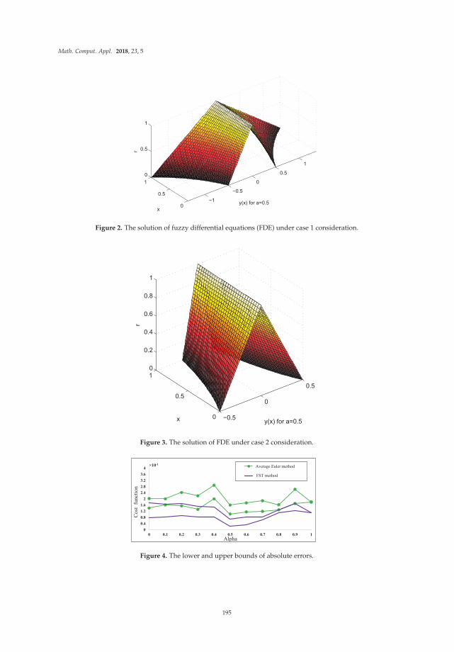
Math. Comput. Appl. 2018, 23, 5
−1
−0.5
0
0.5
1
0
0.5
1
0
0.5
1
y(x) for a=0.5
x
r
Figure 2. The solution of fuzzy differential equations (FDE) under case 1 consideration.
−0.5
0
0.5
0
0.5
10
0.2
0.4
0.6
0.8
1
y(x) for a=0.5x
r
Figure 3. The solution of FDE under case 2 consideration.
[22] Lower
NN Upper
Alpha
Cos
tfu
nctio
n
Average Euler method
FST method
Figure 4. The lower and upper bounds of absolute errors.
195

Math. Comput. Appl. 2018, 23, 5
Example 2. A tank system is displayed in Figure 5. Suppose I = t + 1 is inflow disturbances of the tank thatgenerates vibration in liquid level φ, also H = 1 is the flow obstruction, which can be curbed utilizing the valve.Q = 1 is the cross section of the tank. The liquid level is illustrated as following relation [34],{
φ′(t) = − 1QH φ(t) + I
Q , 0 ≤ t ≤ Tφ(0) = (φ(0, r), φ(0, r))
(71)
By utilizing the FST method we obtain
− S[φ(t)] = (1B� S[φ(t)])� (
1B
S[φ(0)]) (72)
S[φ′(t)](∫ ∞
a1
φ′(Bt)e−tdt (73)
Figure 5. Liquid tank system.
The following relation is extracted by taking into consideration case 2
S[φ′(t)] = (−1B
� S[φ(t)])� (−1B
S[φ(0)]) (74)
So− S[φ(t)] + S[t] + S[1] = (
−1B
� S[φ(t)])� (−1B
S[φ(0)]) (75)
Based on the Equation (42), we have{−S[φ(t, r)] + S[t] + S[1] = 1
B S[φ(t, r)]− 1B φ(0, r)
−S[φ(t, r)] + S[t] + S[1] = 1B S[φ(t, r)]− 1
B φ(0, r)(76)
Therefore, the solution of Equation (76) is extracted as{S[φ(t, r)] = S[t] + S[1] + −1
B S[φ(t, r)]− 1B φ(0, r)
S[φ(t, r)] = S[t] + S[1] + 1B S[φ(t, r)]− 1
B φ(0, r)(77)
hence, {S[φ(t, r)] = ( 1
B+1 )φ(0, r) + BS[φ(t, r)] = ( 1
B+1 )φ(t, r) + B(78)
196

Math. Comput. Appl. 2018, 23, 5
By utilizing the inverse Sumudu transform, we obtain{φ(t, r) = φ(0, r)S−1( 1
B+1 ) + S−1(B)φ(t, r) = φ(0, r)S−1( 1
B+1 ) + S−1(B)(79)
where {φ(t, r) = e−tφ(0, r) + tφ(t, r) = e−tφ(0, r) + t
(80)
If the initial condition is taken to be a symmetric triangular fuzzy number asφ(0) = (−a(1 − r), a(1 − r)), so {
φ(t, r) = e−t(−a(1 − r)) + tφ(t, r) = e−t(a(1 − r)) + t
(81)
Corresponding solution plot is displayed in Figure 6.
−0.5
0
0.5
1
0
0.5
1
0
0.2
0.4
0.6
0.8
1
y(x) for a=0.5x
r
Figure 6. The solution of FDE under case 2 consideration.
Example 3. The nuclear decay equation can be described as [30],{N′(t) = −λN(t)N(0) = (N(0, r), N(0, r))
(82)
where N(t) is considered to be the number of radionuclides present, λ is state as the decay constant, also N0
is taken to be the initial number of radionuclides. Let N0 be a fuzzy number. By utilizing the FST method thefollowing outcomes can be demonstrated
S[N′(t)] = S[−λN(t)] = −λS[N(t)] (83)
S[N′(t)] =∫ ∞
aN′(st)e−tdt (84)
If N(t) is (ii)-differentiable and case 2 holds, we obtain
S[N′(t)] = (−1B
S[N(t)])� (−1B
N(0)) (85)
197
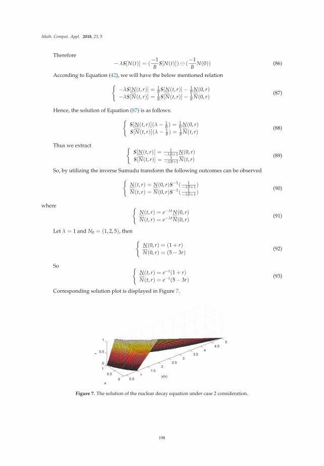
Math. Comput. Appl. 2018, 23, 5
Therefore− λS[N(t)] = (
−1B
S[N(t)])� (−1B
N(0)) (86)
According to Equation (42), we will have the below mentioned relation{−λS[N(t, r)] = 1
B S[N(t, r)]− 1B N(0, r)
−λS[N(t, r)] = 1B S[N(t, r)]− 1
B N(0, r)(87)
Hence, the solution of Equation (87) is as follows:{S[N(t, r)](λ − 1
B ) =1B N(0, r)
S[N(t, r)](λ − 1B ) =
1B N(t, r)
(88)
Thus we extract {S[N(t, r)] = 1
−λB+1 N(0, r)S[N(t, r)] = 1
−λB+1 N(t, r)(89)
So, by utilizing the inverse Sumudu transform the following outcomes can be observed{N(t, r) = N(0, r)S−1( 1
−λB+1 )
N(t, r) = N(0, r)S−1( 1−λB+1 )
(90)
where {N(t, r) = e−λtN(0, r)N(t, r) = e−λtN(0, r)
(91)
Let λ = 1 and N0 = (1, 2, 5), then {N(0, r) = (1 + r)N(0, r) = (5 − 3r)
(92)
So {N(t, r) = e−t(1 + r)N(t, r) = e−t(5 − 3r)
(93)
Corresponding solution plot is displayed in Figure 7.
Figure 7. The solution of the nuclear decay equation under case 2 consideration.
198
Math. Comput. Appl. 2018, 23, 5
6. Conclusions
In this paper, the utilization of FST results in the solution of the first order FDEs in such a mannerthat it is clarified by using the notion of strongly generalized differentiability. By implementing themethodology of FST, the FDE reduces to an algebraic problem. Some theorems are given to illustratethe properties of the FST. The novel method is validated by three real examples. Numerical experimentsalong with comparisons demonstrate the excellent behavior of the proposed method. This work makesa significant contribution in initializing a superior starting point for such extensions. Future workinvolves studying the application of this method in solving FDEs where the uncertainties are in theform of Z-numbers.
Author Contributions: All authors contributed equally to this work. All authors read and approve thefinal manuscript.
Conflicts of Interest: The authors declare no conflict of interest.
References
1. Zwillinger, D. Handbook of Differential Equations; Gulf Professional Publishing: Houston, TX, USA, 1998.2. Khalili Golmankhaneh, A.; Porghoveh, N.; Baleanu, D. Mean square solutions of second-order random
differential equations by using Homotopy analysis method. Rom. Rep. Phys. 2013, 65, 350–361.3. Buckley, J.J.; Eslami, E.; Feuring, T. Fuzzy Mathematics in Economics and Engineering; Physica-Verlag:
Heidelberg, Germany, 2002.4. Diamond, P.; Kloeden, P. Metric Spaces of Fuzzy Sets: Theory and Applications; World Scientific: Singapore, 1994.5. Kloeden, P. Remarks on Peano-like theorems for fuzzy differential equations. Fuzzy Set Syst. 1991, 44, 161–164.6. Jafari, R.; Yu, W. Fuzzy Control for Uncertainty Nonlinear Systems with Dual Fuzzy Equations. J. Intell.
Fuzzy Syst. 2015, 29, 1229–1240.7. Jafari, R.; Yu, W. Fuzzy Differential Equation for Nonlinear System Modeling with Bernstein Neural
Networks. IEEE Access 2016, doi:10.1109/ACCESS.2017.2647920.8. Jafari, R.; Yu, W. Uncertainty Nonlinear Systems Modeling with Fuzzy Equations. Math. Probl. Eng. 2017,
doi :10.1155/2017/8594738.9. Jafarian, A.; Jafari, R. Approximate solutions of dual fuzzy polynomials by feed-back neural networks. J. Soft
Comput. Appl. 2012, doi:10.5899/2012/jsca-00005.10. Jafari, R.; Yu, W.; Li, X.; Razvarz, S. Numerical Solution of Fuzzy Differential Equations with Z-numbers
Using Bernstein Neural Networks. Int. J. Comput. Int. Sys. 2017, 10, 1226–1237.11. Jafari, R.; Yu, W.; Li, X. Numerical solution of fuzzy equations with Z-numbers using neural networks.
Intell. Autom. Soft Comput. 2017, 1–7, doi:10.1080/10798587.2017.1327154.12. Friedman, M.; Ming, M.; Kandel, A. Numerical solution of fuzzy differential and integral equations.
Fuzzy Set Syst. 1999, 106, 35–48.13. Allahviranloo, T.; Ahmadi, M.B. Fuzzy Laplace Transform. Soft Comput. 2010, 14, 235–243.14. Ding, Z.; Ma, M.; Kandel, A. Existence of the solutions of fuzzy differential equations with parameters.
Inf. Sci. 1997, 99, 205–217.15. Truong, V.A.; Ngo, V.H.; Nguyen, D.P. Global existence of solutions for interval-valued integro-differential
equations under generalized H-differentiability. Adv. Differ. Equ. 2013, 1, 217–233.16. Asiru, M.A. Further properties of the Sumudu transform and its applications. Int. J. Math. Educ. Sci. Tech.
2002, 33, 441–449.17. Belgacem, F.B.M.; Karaballi, A.A.; Kalla, S.L. Analytical investigations of the Sumudu transform and
applications to integral production equations. Math. Probl. Eng. 2003, 103, 103–118.18. Deakin, M.A.B. The Sumudu transform and the Laplace transform. Int. J. Math. Educ. Sci. Technol. 1997, 28,
159–160.19. Eltayeb, H.; Kilicman, A. A note on the Sumudu transforms and differential equations. Appl. Math. Sci. 2010,
4, 1089–1098.20. Srivastava, H.M.; Khalili Golmankhaneh, A.; Baleanu, D.; Yang, X.J. Local Fractional Sumudu Transform
with Application to IVPs on Cantor Sets. Abstr. Appl. Anal. 2014, doi:10.1155/2014/620529.
199

Math. Comput. Appl. 2018, 23, 5
21. Abdul Rahman, N.A.; Ahmad, M.Z. Fuzzy Sumudu transform for solving fuzzy partial differential equations.J. Nonlinear Sci. Appl. 2016, 9, 3226–3239.
22. Belgacem, F.B.M.; Karaballi, A.A. Sumudu transform fundamental properties investigations and applications.J. Appl. Math. Stoch. Anal. 2006, doi:10.1155/JAMSA/2006/91083.
23. Liu, Y.; Chen, W. A new iterational method for ordinary equations using Sumudu transform. Adv. Anal.2016, doi:10.22606/aan.2016.12004.
24. Jafari, R.; Razvarz, S. Solution of Fuzzy Differential Equations using Fuzzy Sumudu Transforms. IEEE Int.Conf. Innov. Intell. Syst. Appl. 2017, doi:10.1109/INISTA.2017.8001137.
25. Bede, B.; Stefanini, L. Generalized differentiability of fuzzy-valued functions. Fuzzy Set Syst. 2013, 230, 119–141.26. Seikkala, S. On the fuzzy initial value problem. Fuzzy Set Syst. 1987, 24, 319–330.27. Puri, M.L.; Ralescu, D. Fuzzy random variables. J. Math. Anal. Appl. 1986, 114, 409–422.28. Wu, H.-C. The improper fuzzy Riemann integral and its numerical integration. Inform. Sci. 1999, 111, 109–137.29. Bede, B.; Gal, S.G. Generalizations of the differentiability of fuzzy-number-valued functions with applications
to fuzzy differential equations. Fuzzy Set Syst. 2005, 151, 581–599.30. Bede, B.; Rudas, I.J.; Bencsik, A.L. First order linear fuzzy differential equations under generalized
differentiability. Inf. Sci. 2006, 177, 1648–1662.31. Chalco-Cano, Y.; Roman-Flores, H. On new solutions of fuzzy differential equations. Chaos Solitons Fractals
2006, 38, 112–119.32. Pletcher, R.H.; Tannehill, J.C.; Anderson, D. Computational Fluid Mechanics and Heat Transfer; Taylor and
Francis: Abingdon, UK, 1997.33. Tapaswini, S.; Chakraverty, S. Euler-based new solution method for fuzzy initial value problems. Int. J. Artif.
Intell. Soft Comput. 2014, 4, 58–79.34. Streeter, V.L.; Wylie, E.B.; Bedford, K.W. Fluid Mechanics; McGraw Hill: New York, NY, USA, 1998.
c© 2018 by the authors. Licensee MDPI, Basel, Switzerland. This article is an open accessarticle distributed under the terms and conditions of the Creative Commons Attribution(CC BY) license (http://creativecommons.org/licenses/by/4.0/).
200

Mathematical
and Computational
Applications
Article
A Simple Spectral Observer
Lizeth Torres 1,∗ ID , Javier Jiménez-Cabas 2, José Francisco Gómez-Aguilar 3 ID
and Pablo Pérez-Alcazar 4 ID
1 Cátedras CONACYT, Instituto de Ingeniería, Universidad Nacional Autónoma de México,04510 Ciudad de México, México
2 Departamento de Ciencias de la Informática y Electrónica, Universidad de la Costa,Barranquilla, Colombia; [email protected]
3 Cátedras CONACYT, Centro Nacional de Investigación y Desarrollo Tecnológico,Tecnológico Nacional de México, 62490 Cuernavaca, México; [email protected]
4 Facultad de Ingeniería, Universidad Nacional Autónoma de México, 04510 Ciudad de México, México;[email protected]
* Correspondence: [email protected]
Received: 3 March 2018; Accepted: 10 April 2018; Published: 1 May 2018
Abstract: The principal aim of a spectral observer is twofold: the reconstruction of a signal of timevia state estimation and the decomposition of such a signal into the frequencies that make it up.A spectral observer can be catalogued as an online algorithm for time-frequency analysis because is amethod that can compute on the fly the Fourier Transform (FT) of a signal, without having the entiresignal available from the start. In this regard, this paper presents a novel spectral observer with anadjustable constant gain for reconstructing a given signal by means of the recursive identification ofthe coefficients of a Fourier series. The reconstruction or estimation of a signal in the context of thiswork means to find the coefficients of a linear combination of sines a cosines that fits a signal suchthat it can be reproduced. The design procedure of the spectral observer is presented along with thefollowing applications: (1) the reconstruction of a simple periodical signal, (2) the approximation ofboth a square and a triangular signal, (3) the edge detection in signals by using the Fourier coefficients,(4) the fitting of the historical Bitcoin market data from 1 December 2014 to 8 January 2018 and (5) theestimation of a input force acting upon a Duffing oscillator. To round out this paper, we presenta detailed discussion about the results of the applications as well as a comparative analysis of theproposed spectral observer vis-à-vis the Short Time Fourier Transform (STFT), which is a well-knownmethod for time-frequency analysis.
Keywords: signal processing; Fourier series; state observer; Short Time Fourier Transform;time-frequency analysis
1. Introduction
The term spectral observer was proposed by Hostetter in his pioneering work [1] to name thealgorithm that permits the recursive calculation of the Fourier Transform (FT) of a band-limited signalvia state estimation. Since the presentation of such a work, several designs of spectral observers withimproved features have been proposed either to deal with noise [2], disturbances, lack of data [3] or toestimate other parameters such as frequency [4]. The main goals of a spectral observer are both theestimation of a given signal and the transformation of such a signal to the frequency domain by meansof the recursive identification of the coefficients of a Fourier series [5]. The estimation of a signal in thecontext of this work means to find the coefficients of a linear combination of functions—sines a cosinesfunctions in our case—that approximates a signal of interest such that it can be reconstructed [6].Spectral observers are useful in a wide number of applications, e.g., for determining the source of
Math. Comput. Appl. 2018, 2, 23; doi:10.3390/mca23020023 www.mdpi.com/journal/mca201

Math. Comput. Appl. 2018, 2, 23
harmonic pollution in power systems [7], for the simulation of the sea surface [8], for fault diagnosis inmotors [9,10] or in vibrating structures, such as aerospace and mechanical structures, marine structures,buildings, bridges and offshore platforms.
A spectral observer can be catalogued as an online algorithm to compute the FourierTransform (FT) during a time window which slides along the signal, i.e., an algorithm to compute theShort Time Fourier Transform (STFT). Therefore, a spectral observer can be used for the time-frequencyanalysis of frequency variant signals.
The observer that we propose in this contribution is designed from a dynamical system which isconstructed from the N derivatives of a n-th order Fourier series.
To perform the estimation, the observer solely requires: (1) The measurement of the signal tobe approximated, s(t), which actually is used to compute the observation error e(t) = s(t)− y(t),where y(t) is the observer output, (2) A frequency step ω = 2π/T, where T is a predefined period.The estimation provided by the observer are both the reconstruction of the original signal and theFourier coefficients to compute the signal frequency components.
This paper is organized as follows: Section 2 presents the core of the proposed method which isthe formulation of the spectral observer from the Fourier series. Section 3 presents some exampleswith test results of the proposed method utilized in different applications. In Section 4 the main resultsare discussed. Finally, in Section 5 some concluding thoughts are given.
2. The Proposed Method
To construct the proposed observer, we formulate a dynamical synthetic system in state spacerepresentation by considering, firstly, that a given signal expressed as s(t) can be approximated by aFourier series, and secondly, that the Fourier series is the first state of the system and the rest of thestates are the N first-order derivatives of the Fourier series expressed by Equation (1), where n is theseries order.
y(t) =a0
2+
n
∑k=1
[ak cos (kωt) + bk sin (kωt)] , (1)
where a0, a1, b1, ..., an, bn are the Fourier coefficients and ω is the fundamental angular frequency of thesignal to be estimated.
In this work, we assume that the signal s(t) to be approximated has not a constant component(offset) or that this offset is removed by an online algorithm prior to be processed by the spectralobserver. For this reason, we remove the term a0 from Equation (1) such that the series forapproximating the time function s(t) can be expressed as follows
y(t) =n
∑k=1
[ak cos (kωt) + bk sin (kωt)] . (2)
If the order of the Fourier series is n = 1, we need to formulate a dynamical system with N = 2states, each one to recover each coefficient (a1 and b1). Thus, the two first states are the Fourier seriesand its first derivative.
ν1(t) = y(t) = a1 cos (ωt) + b1 sin (ωt), ν2(t) = y(t) = −ωa1 sin (ωt) + ωb1 cos (ωt). (3)
where νi are the states of the synthetic system. Consequently, the dynamical system that results fromthe change of coordinates, gives:
ν1(t) = ν2(t), ν2(t) = −ω2ν1(t), (4)
202

Math. Comput. Appl. 2018, 2, 23
which basically is the dynamical model of a harmonic oscillator. Now, what happens if the order ofthe Fourier series increases? If the order increases to n = 2, then N = 4, since we need to recoverfour coefficients.
ν1(t) = y(t) = a1 cos (ωt) + b1 sin (ωt) + a2 cos (2ωt) + b2 sin (2ωt),
ν2(t) = y(t) = −ωa1 sin (ωt) + ωb1 cos (ωt)− 2ωa2 sin (2ωt) + 2ωb2 cos (2ωt),
ν3(t) = y(t) = −ω2a1 cos (ωt)− ω2b1 sin (ωt)− 4ω2a2 cos (2ωt)− 4ω2b2 sin (2ωt), (5)
ν4(t) = y(3)(t) = ω3a1 sin (ωt)− ω3b1 cos (ωt) + 8ω3a2 sin (2ωt)− 8ω3b2 cos (2ωt),
ν4(t) = y(4)(t) = ω4a1 cos (ωt) + ω4b1 sin (ωt) + 16ω4a2 cos (2ωt) + 16ω4b2 sin (2ωt).
The dynamical system is then formulated as in Equation (5) which, after some algebraicmanipulations, it becomes
ν1(t) = ν2(t); ν2(t) = ν3(t), ν3(t) = ν4(t), ν4(t) = −4ω4ν1(t)− 5ω2ν3(t), (6)
in ν-coordinates.By generalizing Equation (5) for order n, we obtain the following dynamical system:
ν1(t) = ν2(t),
ν2(t) = ν3(t),... =
..., (7)
νN(t) = (−1)n(mod 2)ω2n[1 22n · · · n2n
]A−1
k A−1ω ν(t),
where N = 2n, Aω and Ak are expressed by Equations (8) and (9), respectively.
Aω.=
⎡⎢⎢⎢⎢⎢⎢⎢⎢⎢⎢⎢⎢⎢⎢⎣
1 0 0 0 · · · 0 · · · 00 ω 0 0 · · · 0 · · · 00 0 −ω2 0 · · · 0 · · · 00 0 0 −ω3 · · · 0 · · · 0...
......
.... . .
.... . .
...0 0 0 0 · · · (−1)(m(mod 4)−m(mod 2))/2 ωm · · · 0...
......
.... . .
.... . .
...0 0 0 0 · · · 0 · · · (−1)(2n(mod 4)−2)/2 ω2n−1
⎤⎥⎥⎥⎥⎥⎥⎥⎥⎥⎥⎥⎥⎥⎥⎦, (8)
Ak.=
⎡⎢⎢⎢⎢⎢⎢⎢⎢⎢⎢⎣
1 0 1 0 · · · 1 00 1 0 2 · · · 0 n1 0 4 0 · · · n2 00 1 0 8 · · · 0 n3
......
......
. . ....
...1 0 22n−2 0 · · · n2n−2 00 1 0 22n−1 · · · 0 n2n−1
⎤⎥⎥⎥⎥⎥⎥⎥⎥⎥⎥⎦. (9)
Before presenting the state observer for system (7), it is necessary to analyze its observabilityconditions. A dynamical system is said to be observable if it is possible to determine its initial state byknowledge of the input and output over a finite time interval. In this way, a state observer or stateestimator is a system that estimates the internal states of a system from the measurement of its inputsand outputs. To verify is a linear systems is observable, the observability rank condition can be used,which is defined in the net lines.
203
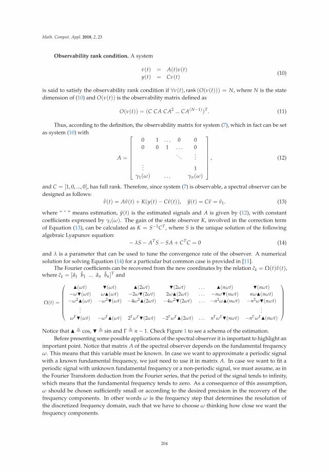
Math. Comput. Appl. 2018, 2, 23
Observability rank condition. A system
ν(t) = A(t)ν(t)y(t) = Cν(t)
(10)
is said to satisfy the observability rank condition if ∀ν(t), rank (O(ν(t))) = N, where N is the statedimension of (10) and O(ν(t)) is the observability matrix defined as
O(ν(t)) = (C CA CA2 ... CA(N−1))T . (11)
Thus, according to the definition, the observability matrix for system (7), which in fact can be setas system (10) with
A =
⎡⎢⎢⎢⎢⎢⎢⎢⎣
0 1 . . . 0 00 0 1 . . . 0
. . ....
... 1γ1(ω) . . . γn(ω)
⎤⎥⎥⎥⎥⎥⎥⎥⎦, (12)
and C = [1, 0, ..., 0], has full rank. Therefore, since system (7) is observable, a spectral observer can bedesigned as follows:
˙ν(t) = Aν(t) + K(y(t)− Cν(t)), y(t) = Cν = ν1. (13)
where “ ˆ ” means estimation, y(t) is the estimated signals and A is given by (12), with constantcoefficients expressed by γi(ω). The gain of the state observer K, involved in the correction termof Equation (13), can be calculated as K = S−1CT , where S is the unique solution of the followingalgebraic Lyapunov equation:
− λS − ATS − SA + CTC = 0 (14)
and λ is a parameter that can be used to tune the convergence rate of the observer. A numericalsolution for solving Equation (14) for a particular but common case is provided in [11].
The Fourier coefficients can be recovered from the new coordinates by the relation ck = Ω(t)ν(t),where ck = [a1 b1 ... an bn]T and
Ω(t) =
⎛⎜⎜⎜⎜⎜⎜⎝
�(ωt) �(ωt) �(2ωt) �(2ωt) . . . �(nωt) �(nωt)−ω�(ωt) ω�(ωt) −2ω�(2ωt) 2ω�(2ωt) . . . −nω�(nωt) nω�(nωt)−ω2�(ωt) −ω2�(ωt) −4ω2�(2ωt) −4ω2�(2ωt) . . . −n2ω�(nωt) −n2ω�(nωt)
......
ωΓ�(ωt) −ωΓ�(ωt) 2ΓωΓ�(2ωt) −2ΓωΓ�(2ωt) . . . nΓωΓ�(nωt) −nΓωΓ�(nωt)
⎞⎟⎟⎟⎟⎟⎟⎠Notice that � � cos, � � sin and Γ � n − 1. Check Figure 1 to see a schema of the estimation.
Before presenting some possible applications of the spectral observer it is important to highlight animportant point. Notice that matrix A of the spectral observer depends on the fundamental frequencyω. This means that this variable must be known. In case we want to approximate a periodic signalwith a known fundamental frequency, we just need to use it in matrix A. In case we want to fit aperiodic signal with unknown fundamental frequency or a non-periodic signal, we must assume, as inthe Fourier Transform deduction from the Fourier series, that the period of the signal tends to infinity,which means that the fundamental frequency tends to zero. As a consequence of this assumption,ω should be chosen sufficiently small or according to the desired precision in the recovery of thefrequency components. In other words ω is the frequency step that determines the resolution ofthe discretized frequency domain, such that we have to choose ω thinking how close we want thefrequency components.
204

Math. Comput. Appl. 2018, 2, 23
ˆ( ) ( )kc t t
1ˆ( ) ( )y t t
( ): Signal Estimated signal State Observer
1 1ˆˆ ˆ ˆ[ ... ]T
k n nc a b a b
Figure 1. Schema of the reconstruction of a signal by using the spectral observer.
3. Application Examples
This section presents five examples of possible applications of the spectral observer, which wereconceived such that the reader can be able to reproduce them.
3.1. Example 1: A Simple Example
Let be the signal s(t) = 4 cos (t) + sin (t) + 2 cos (2t) + 5 sin (2t). It is obvious that the series orderto reproduce the signal is n = 2, then the order of system (7) for the conception of the observer shouldbe N = 4. Figure 2 shows the estimation of the coefficients that was performed by the observer with again λ = 8, which actually was initialized with ν(0) = 0. The step time to perform the estimation inSimulink was Δt = 0.005 [s] and the used solver was ODE3.
0 2 4 6 8 10 12 14 16 18 20−2
−1
0
1
2
3
4
5
6
7
[s]
a1b1a2b2
Figure 2. Example 1. Estimated coefficients.
3.2. Example 2: Reconstruction of Basic Signals
This example aims to show the estimation of the coefficients for basic signals such as square andsawtooth waves. The first signal to be estimated is a square wave with angular frequency ω = 1[rad/s]. The observer was tuned with λ = 15. The order of the series was set n = 2, i.e., N = 4.The frequency step was set ω = 5 [rad/s]. The step time to perform the estimation in Simulink was setΔt = 0.01 [s] and the used solver was ODE3. Figure 3 shows the signal reconstruction performed bythe spectral observer and the estimated coefficients. Firstly, notice that the coefficients do not convergetowards a constant value; the reason for this is the number of coefficients used to approximate thesignal, which is not enough to represent each harmonic that composes it. Even though the coefficientsare not constant, the signal is estimated. Notice too that all the coefficients change abruptly at eachdiscontinuity. This feature can be used for edge detection as will be seen in the next example.
205

Math. Comput. Appl. 2018, 2, 23
y(t)y(t)
a1b1a2b2
Figure 3. Example 2. (a) Square wave reconstruction and (b) Estimated coefficients.
Both the observer and conditions that were used to reconstruct the square wave were used toreconstruct the sawtooth signal shown in Figure 4. Notice that the convergence time is less than onesecond and the coefficients become greater at the discontinuities.
0 1 2 3 4 5 6 7 8 9 10 11 12 13 14 15−2
−1
0
1
2(a)
0 1 2 3 4 5 6 7 8 9 10 11 12 13 14 15−40−30−20−10
010203040
[s]
(b)
s(t)y(t)
a1 b1 a2 b2
Figure 4. Example 2. (a) Triangular wave reconstruction and (b) Estimated coefficients.
To end this example, we made several simulations to show how the parameter λ determines theconvergence period of the estimation. Figure 5 shows the estimation of the square signal with differentvalues of λ. Notice that the bigger its value, the faster is the convergence.
206
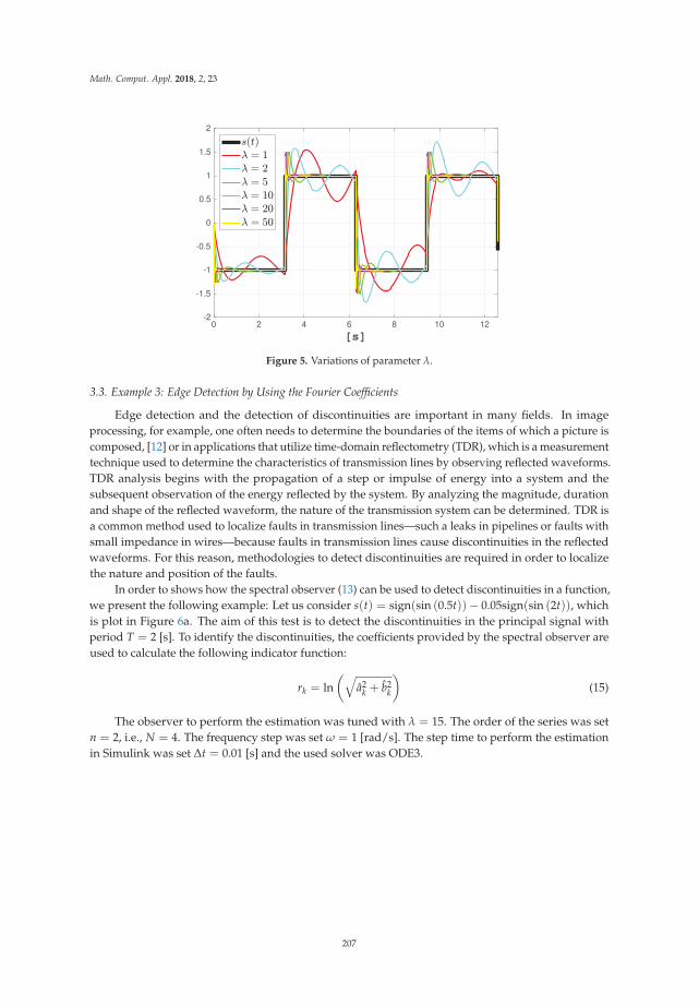
Math. Comput. Appl. 2018, 2, 23
0 2 4 6 8 10 12
[s]
-2
-1.5
-1
-0.5
0
0.5
1
1.5
2
Figure 5. Variations of parameter λ.
3.3. Example 3: Edge Detection by Using the Fourier Coefficients
Edge detection and the detection of discontinuities are important in many fields. In imageprocessing, for example, one often needs to determine the boundaries of the items of which a picture iscomposed, [12] or in applications that utilize time-domain reflectometry (TDR), which is a measurementtechnique used to determine the characteristics of transmission lines by observing reflected waveforms.TDR analysis begins with the propagation of a step or impulse of energy into a system and thesubsequent observation of the energy reflected by the system. By analyzing the magnitude, durationand shape of the reflected waveform, the nature of the transmission system can be determined. TDR isa common method used to localize faults in transmission lines—such a leaks in pipelines or faults withsmall impedance in wires—because faults in transmission lines cause discontinuities in the reflectedwaveforms. For this reason, methodologies to detect discontinuities are required in order to localizethe nature and position of the faults.
In order to shows how the spectral observer (13) can be used to detect discontinuities in a function,we present the following example: Let us consider s(t) = sign(sin (0.5t))− 0.05sign(sin (2t)), whichis plot in Figure 6a. The aim of this test is to detect the discontinuities in the principal signal withperiod T = 2 [s]. To identify the discontinuities, the coefficients provided by the spectral observer areused to calculate the following indicator function:
rk = ln(√
a2k + b2
k
)(15)
The observer to perform the estimation was tuned with λ = 15. The order of the series was setn = 2, i.e., N = 4. The frequency step was set ω = 1 [rad/s]. The step time to perform the estimationin Simulink was set Δt = 0.01 [s] and the used solver was ODE3.
207

Math. Comput. Appl. 2018, 2, 23
0 1 2 3 4 5 6 7 8 9 10 11 12 13 14 15−2
−1
0
1
2(a)
0 1 2 3 4 5 6 7 8 9 10 11 12 13 14 15−10
−5
0
5
10(b)
[s]
s(t)y(t)
r1 = ln
(√a21 + b21
)r2 = ln
(√a22 + b22
)
Figure 6. Example 3. (a) Signal reconstruction and (b) Estimated coefficients.
Figure 6a shows s(t) and its reconstruction y(t). Figure 6b shows the index r1(t) and r2(t) thatbecomes greater at the discontinuities indicating where they are.
3.4. Example 4: Fitting Complex Signal: The Bitcoin Price
Bitcoin is the longest running and best known cryptocurrency in the world. It was released asopen source in 2009 by the anonymous Satoshi Nakamoto. Bitcoin serves as a decentralized medium ofdigital exchange, with transactions verified and recorded in a public distributed ledger (the blockchain)without the need for a trusted record keeping authority or central intermediary. Hereafter, we willuse the proposed spectral observer for fitting the historical Bitcoin market close data every 1000 [min].The records were downloaded from the website: https://www.kaggle.com/neelneelpurk/bitcoin/data.
The observer to perform the estimation was tuned with λ = 1. The order of the series was setn = 20, i.e., N = 40. The frequency step was set ω = 10 [rad/s]. The step time to perform theestimation in Simulink was set Δt = 0.01 [s] and the used solver was ODE8.
In Figure 7, the Bitcoin fitting performed by the spectral observer is shown. Figure 8 showsthe estimated coefficients which are not constant and look as if they were enveloped by exponentialfunctions. In order to have a model that represents the behavior of the Bitcoin in the specified interval,we can fit each coefficient by means of polynomials after calculating the natural logarithm of each one.In Figure 9, ln (|a1|) is plotted versus a cubic polynomial calculated to interpolate it.
ln (|a1|) = 1.2 × 10⁻⁹t3 + 1.5 × 10⁻⁶t2 − 0.0021t − 1.4, (16)
We can perform the same procedure for each coefficient to obtain a series with the following form:
y(t) =(
e|(αc1t3+βc1t2+γc1t+δc1)|)
cos (ωt) +(
e|(αs1t3+βs1t2+γs1t+δs1)|)
sin (ωt)
+(
e|(αc2t3+βc2t2+γc2t+δc2)|)
cos (2ωt) +(
e|(αs2t3+βs2t2+γs2t+δs2)|)
sin (2ωt) (17)
+... +(
e|(αcnt3+βcnt2+γcnt+δcn)|)
cos (nωt) +(
e|(αsnt3+βsnt2+γsnt+δsn)|)
sin (nωt)
where αck, βck, γck, δck, αsk, βsk, γsk, δsk are the coefficients of the polynomial that approximates thenatural logarithms of the coefficients.
208
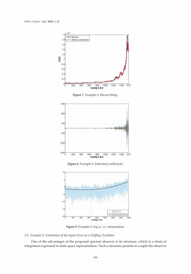
Math. Comput. Appl. 2018, 2, 23
0 200 400 600 800 1000 1200 1400 15770
0.2
0.4
0.6
0.8
1
1.2
1.4
1.6
1.8
2x 10
4
samples
USD
BitcoinBitcoin estimation
Figure 7. Example 4. Bitcoin fitting.
0 200 400 600 800 1000 1200 1400 1577−500
−300
−100
100
300
500
samples
Figure 8. Example 4. Estimated coefficients.
0 200 400 600 800 1000 1200 1400 1600−20
−15
−10
−5
0
5
10
samples
ln (|a1|)Interpolation
Figure 9. Example 4. log |a1| vs. interpolation.
3.5. Example 5: Estimation of the Input Force on a Duffing Oscillator
One of the advantages of the proposed spectral observer is its structure, which is a chain ofintegrators expressed in state-space representation. Such a structure permits to couple the observer
209

Math. Comput. Appl. 2018, 2, 23
to dynamic models, also expressed in state variables, that represent physical systems for control orestimation purposes. With this in mind, we present an example to show how the spectral observer canbe coupled to the model of a given system, even with nonlinear structure such as the Duffing oscillator,in order to estimate an exogenous input affecting its behavior.
The Duffing oscillator is expressed by the following equation:
x(t) + δx(t) + αx(t) + βx3(t) = u(t) (18)
where x(t) is the displacement, which is assumed as available in this example, x(t) is the velocity andx(t) is the acceleration. In addition, δ, α and β are parameters, which in this example are assumedto be known. Finally, u(t) is an external force, which is unknown and can be estimated by using ourproposed observer. To achieve this goal, the following steps need to be executed.
Step 1. Equation (18) must be set in state-space representation. To execute this step, we definex1(t) = x(t) and x2(t) = x(t) as the state variables, such that we obtain the following equation system:
x1(t) = x2(t),
x2(t) = −δx2(t)− αx(t)− βx3(t) + u(t), (19)
y(t) = x1(t).
If the Liénard transform [13] is applied to system (18) in order to set it in a more appropriate formfor estimation purposes [14], it becomes
x1(t) = x2(t)− δx1(t),
x2(t) = −αx1(t)− βx31(t) + u(t), (20)
Step 2. Since u(t) is unknown and needs to be estimated, we propose its estimation by using aspectral observer with n = 1. Therefore, we coupled in cascade equation system (18) with equationsystem (4) as follows:
x1(t) = x2(t)− δx1(t),
x2(t) = −αx1(t)− βx31(t) + ν1(t), (21)
ν1(t) = ν2(t),
ν2(t) = −ω2ν1(t),
y(t) = x1(t),
where ν1(t) = u(t), i.e., it is the force to be estimated.System (21) can be set in the following form:⎛⎜⎜⎜⎝
x1(t)x2(t)ν1(t)ν2(t)
⎞⎟⎟⎟⎠︸ ︷︷ ︸
ξ(t)
=
⎛⎜⎜⎜⎝0 1 0 00 0 1 00 0 0 10 0 −ω2 0
⎞⎟⎟⎟⎠︸ ︷︷ ︸
A
⎛⎜⎜⎜⎝x1(t)x2(t)ν1(t)ν2(t)
⎞⎟⎟⎟⎠︸ ︷︷ ︸
ξ(t)
+
⎛⎜⎜⎜⎝−δy(t)
−αy(t)− βy3(t)00
⎞⎟⎟⎟⎠ ,
︸ ︷︷ ︸ϕ(ξ(t))
(22)
y(t) = [1 0 0 0]ξ(t) = Cξ(t) = x1(t), (23)
which according to [15] is uniformly observable. Therefore, a state observer expressed asˆξ(t) = A ˆξ(t) + ϕ( ˆξ(t)) + K(x1(t)− ξ1(t)) can be designed for system (22), where K can be calculatedby means of Equation (14).
For the simulation, the paramaters of the Duffing oscillator were set: α = 1, β = 1 and δ = 0.3;and their initial conditions were set x(0) = [−1 − 5]. The force applied to the oscillator was
210

Math. Comput. Appl. 2018, 2, 23
u(t) = 2 cos (2t) + 5 sin (2t) + 4 sin (0.5t). The observer was tuned with λ = 10, ω = 1 [rad/s]and their initial conditions were fixed as ξ(0) = [0 0 0 0]. Finally, the used solver was ODE 3 witha step time Δt = 0.01 [s]. The results of the estimation are shown in Figure 10, which particularlypresents a comparison between the force and its estimation. Notice that the estimation converges tothe force in 1 [s].
10-2 10-1 100 101
[s]
-100
-80
-60
-40
-20
0
20
40
Figure 10. Example 5. Force estimation.
4. Comparative Analysis Vis-à-Vis the STFT
A spectral observer can be used to determine the frequency content of local sections of a signal asit changes over time. The classic technique for performing this task is the Short Time Fourier Transform,which is the Fourier Transform with a suitable chosen windowing function. Ensuing, we present anexample to compare the results of using the STFT with the results provided by the spectral observer.For this purpose, we used the MATLAB c© codes created by Hristo Zhivomirov to compute STFT andits inverse [16]. The signal analyzed was
s(t) =
⎧⎪⎪⎪⎪⎪⎨⎪⎪⎪⎪⎪⎩
0 0 ≤ t < 100[s]sin (10πt) 0 ≤ t < 300[s]0 300 ≤ t < 400[s]sin (4πt) 400 ≤ t < 600[s]0 600 ≤ t < 700[s]
(24)
sampled at 1000 [Hz]. To compute the STFT by using the code of Zhivomirov, the following parameterswere set: τw = 28 [s] as the window length, h = τw/4 [s] as the hop size and n f f t = 210 as the numberof FFT points. The tuning of the spectral observer was done by setting n = 10, λ = 1, ω = π [rad/s]and ν(0) = 0. The solver used for the numerical solution was ODE4 (Runge-Kutta) with a fixedstep size Δt = 0.01 [s]. The spectrograms that were produced by the STFT and the spectral observer,respectively, are presented in Figure 11. To construct the observer spectrogram, we computed demagnitude of each harmonic by means of the following equation:
|Ak| =√
ak + bk. (25)
On the one hand, since n = 10, the resulting vector containing the magnitude of each harmonicwas A = [A1 A2 A3 A4 A5 A6 A7 A8 A9 A10]. On the other hand, since the angular frequency stepwas chosen ω = π [rad/s], the resulting frequency vector was f = [0.5 1 1.5 2 2.5 3 3.5 4 4.5 5] [Hz].Then, the spectrogram resulted of plotting f versus A.
Notice that the spectrogram generated by using the spectral observer presents a better frequencyresolution with respect to the spectral observer. This fact can be better appreciated in Figure 12.
211

Math. Comput. Appl. 2018, 2, 23
However, this does not mean that the observer’s performance is superior, since it is well known thatthe frequency resolution can be improved by widening the time window length of the STFT, evenif this widening implies a decreasing of the time resolution. In the case of the spectral observer, thefrequency resolution is adjusted by manipulating the parameter λ.
Figure 11. (a) STFT spectrogram (b) Spectral observer spectrogram.
Figure 12. (a) STFT spectrogram (b) Spectral observer spectrogram.
It is necessary to point out here that both the frequency resolution and the time resolution do notonly depend on the parameters τ and λ, also the parameters h y n f f t used in the STFT algorithm andω and n used in the spectral observer, play an important factor; nevertheless, the adjustment of theseparameters directly affects in the computational burden and the amount of data to be processed.
5. Results and Discussion
We have introduced an algorithm to reconstruct signals at the same time that their frequencycomponents are calculated: a new spectral observer. In order to show its applicability, we havepresented some examples, which in addition, have allowed us to glimpse some advantages anddisadvantages of its use. Firstly, we found the following benefits: (1) The structure of the observer,as a chain of integrators, is very adequate for control and parameter estimation purposes; (2) Thesignal is progressively incorporated at each iteration; (3) The operations required for the observerimplementation are with real numbers, which simplifies its programming in single-board computers;(4) The gain of the observer can be easily computed by means of a simple numerical algorithm; (5) Theconvergence of the observer is exponential, this means that the convergence period can be adjustedby means of a unique parameter λ, which is a clear advantage with respect to other well-knownalgorithms such as the proposed in [17], where the convergence period cannot be manipulated by aunique parameter. However, there are some drawbacks that we have found for the proposed observer.
212

Math. Comput. Appl. 2018, 2, 23
(1) The computational cost can be high for a small frequency resolution; (2) The algorithm must becomplemented with a methodology to choose ω and λ in order to obtain the best estimation.
To conclude the discussion, it is necessary to emphasize that the spectral observer is an algorithmthat, like the STFT, can be used to perform a frequency-time analysis of a frequency varying signalby computing the Fourier Transform (FT) during time intervals. However, there are some differencesto remark. (a) The STFT requires operations with complex numbers, the spectral observer does not;(b) The spectral observer computes the FT and its inverse at the same time, which is a clear bonus,because in case of using a recursive STFT we only get the FT, if we want to recover the reconstructedsignal, we must compute the Inverse Short Fourier Transform.
6. Conclusions
In this paper, we presented the design of a novel spectral observer, which can be used toapproximate periodical and non-periodical signals via state estimation. To design the spectral observer,we constructed a synthetic system in state space representation from the Fourier series. We presentedsome application examples to reconstruct periodical signals but also a well-know non-periodical onesuch as the price of the Bitcoin from its genesis. Some important aspects were not discussed in thisarticle that require a deeper analysis, such as a comparison between the computational burden of thespectral observer and that of the Fourier Transform or an analysis of the spectral observer vis-à-visperturbations and noise. These aspects must be treated in a continuation of this research work.
Author Contributions: Lizeth Torres conceived the spectral observer presented in this article.Javier Jiménez-Cabas and José Francisco Gómez-Aguilar conceived, designed and performed the simulation tests.Pablo Pérez-Alcazar advised the rest of the authors. All the authors wrote the paper.
Conflicts of Interest: The authors declare no conflict of interest.
Appendix A. MATLAB CODES
Appendix A.1. Symbolic Computation of Matrix Aω
syms w tn=10; %Order of the Fourier Seriesfor k=1:2*n;Aw(k,k)=((-1)^((mod(k-1,4)-mod(k-1,2))/2))*w^(k-1);end
Appendix A.2. Symbolic Computation of Matrix Aω
syms w tn=10; %Order of the Fourier Seriesfor k=1:nfor m=1:nAk(2*m-1,2*k-1)=k^(2*m-2);Ak(2*m,2*k)=k^(2*m-1);endend
Appendix A.3. Symbolic Computation of Matrix Ω
syms w tn=10; %Order of the Fourier Seriesfor k=1:nfor m=2:2*nO(1,(2*k)-1)=cos(k*w*t);O(1,(2*k))=sin(k*w*t);
213

Math. Comput. Appl. 2018, 2, 23
O(m,(2*k)-1)=diff(O(m-1,2*k-1),’t’);O(m,(2*k))=diff(O(m-1,2*k),’t’);endend
References
1. Hostetter, G.H. Recursive discrete Fourier transformation. IEEE Trans. Acoust. Speech Signal Proc. 1980,28, 184–190. [CrossRef]
2. Bitmead, R.R.; Tsoi, A.C.; Parker, P.J. A Kalman filtering approach to short-time Fourier analysis. IEEE Trans.Acoust. Speech Signal Proc. 1986, 34, 1493–1501. [CrossRef]
3. Orosz, G.; Sujbert, L.; Peceli, G. Spectral observer with reduced information demand. In Proceedings of the2008 IEEE Instrumentation and Measurement Technology Conference, Victoria, BC, Canada, 12–15 May 2008;pp. 2155–2160.
4. Na, J.; Yang, J.; Wu, X.; Guo, Y. Robust adaptive parameter estimation of sinusoidal signals. Automatica 2015,53, 376–384. [CrossRef]
5. Bitmead, R.R. On recursive discrete Fourier transformation. IEEE Trans. Acoust. Speech Signal Proc. 1982,30, 319–322. [CrossRef]
6. Torres, L.; Gómez-Aguilar, J.; Jiménez, J.; Mendoza, E.; López-Estrada, F.; Escobar-Jiménez, R. Parameteridentification of periodical signals: Application to measurement and analysis of ocean wave forces.Digit. Signal Proc. 2017, 69, 59–59. [CrossRef]
7. Dash, P.K.; Khincha, H. New algorithms for computer relaying for power transmission lines. Electr. Mach.Power Syst. 1988, 14, 163–178. [CrossRef]
8. Houmb, O.; Overvik, T. Some applications of maximum entropy spectral estimation to ocean waves andlinear systems response in waves. Appl. Ocean Res. 1981, 3, 154–162. [CrossRef]
9. Blödt, M.; Chabert, M.; Regnier, J.; Faucher, J. Mechanical load fault detection in induction motors by statorcurrent time-frequency analysis. IEEE Trans. Ind. Appl. 2006, 42, 1454–1463. [CrossRef]
10. Benbouzid, M.E.H.; Vieira, M.; Theys, C. Induction motors’ faults detection and localization using statorcurrent advanced signal processing techniques. IEEE Trans. Power Electron. 1999, 14, 14–22. [CrossRef]
11. Busawon, K.; Farza, M.; Hammouri, H. A simple observer for a class of nonlinear systems. Appl. Math. Lett.1998, 11, 27–31. [CrossRef]
12. Engelberg, S. Edge detection using Fourier coefficients. Am. Math. Mon. 2008, 115, 499–513. [CrossRef]13. Liénard, A. Étude des oscillations entretenues. Revue Générale de l’Électricité 1928, 23, 901–912.14. Torres, L.; Verde, C.; Vázquez-Hernández, O. Parameter identification of marine risers using Kalman-like
observers. Ocean Eng. 2015, 93, 84–97. [CrossRef]15. Hammouri, H. Uniform observability and observer synthesis. In Nonlinear Observers and Applications;
Besançon, G., Ed.; Springer: Berlin, Germany, 2007; pp. 35–70.16. Zhivomirov, H. Short-Time Fourier Transformation (STFT) with Matlab Implementation. Available online:
https://www.mathworks.com/matlabcentral/fileexchange/45197-short-time-fourier-transformation--stft--with-matlab-implementation (accessed on 27 April 2018).
17. Kušljevic, M.D.; Tomic, J.J. Multiple-resonator-based power system Taylor-Fourier harmonic analysis.IEEE Trans. Instrum. Meas. 2015, 64, 554–563. [CrossRef]
c© 2018 by the authors. Licensee MDPI, Basel, Switzerland. This article is an open accessarticle distributed under the terms and conditions of the Creative Commons Attribution(CC BY) license (http://creativecommons.org/licenses/by/4.0/).
214
Mathematical
and Computational
Applications
Article
Differential Evolution Algorithm for MultilevelAssignment Problem: A Case Study inChicken Transportation
Sasitorn Kaewman 1,*, Tassin Srivarapongse 2, Chalermchat Theeraviriya 3 and
Ganokgarn Jirasirilerd 4
1 Faculty of Informatics, Mahasarakham University, Maha Sarakham 44150, Thailand2 Department of Economics, Rajamangala University of Technology Thanyaburi, Patumthani 12110, Thailand;
[email protected] Faculty of Engineering, Nakhon Phanom University, Nakhon Phanom 48000, Thailand;
[email protected] Faculty of Liberal Arts and Sciences, Sisaket Rajabhat University, Sisaket 33000, Thailand;
[email protected]* Correspondence: [email protected]; Tel.: +66-89-861-6143
Received: 12 September 2018; Accepted: 30 September 2018; Published: 2 October 2018
Abstract: This study aims to solve the real-world multistage assignment problem. The proposedproblem is composed of two stages of assignment: (1) different types of trucks are assigned to chickenfarms to transport young chickens to egg farms, and (2) chicken farms are assigned to egg farms.Assigning different trucks to the egg farms and different egg farms to the chicken farms generatesdifferent costs and consumes different resources. The distance and the idle space in the truck have tobe minimized, while constraints such as the minimum number of chickens needed for all egg farmsand the longest time that chickens can be in the truck remain. This makes the problem a special caseof the multistage assignment (S-MSA) problem. A mathematical model representing the problemwas developed and solved to optimality using Lingo v.11 optimization software. Lingo v.11 can solveto optimality only small- and medium-sized test instances. To solve large-sized test instances, thedifferential evolution (DE) algorithm was designed. An excellent decoding method was developedto increase the search performance of DE. The proposed algorithm was tested with three randomlygenerated datasets (small, medium, and large test instances) and one real case study. Each datasetis composed of 12 problems, therefore we tested with 37 instances, including the case study. Theresults show that for small- and medium-sized test instances, DE has 0.03% and 0.05% higher costthan Lingo v.11. For large test instances, DE has 3.52% lower cost than Lingo v.11. Lingo v.11 uses anaverage computation time of 5.8, 103, and 4320 s for small, medium and large test instances, while DEuses 0.86, 1.68, and 8.79 s, which is, at most, 491 times less than Lingo v.11. Therefore, the proposedheuristics are an effective algorithm that can find a good solution while using less computation time.
Keywords: assignment problem; chicken transportation; differential evolution algorithm;mathematical model
1. Introduction
Thailand has long been known as a farming country due to the influence of Southeast Asianmonsoons, which make the landscape, resources, environment, and climate conducive to agriculture.Most of the population works in agriculture or is involved in it in some manner. Although there havebeen efforts to develop Thailand into an industrialized country, it still largely depends on agriculture.The evolution and development of Thai agriculture has changed over time, reflecting the worldwideflow of changes. Hens are considered to be economic animals, as farmers can generate revenue from
Math. Comput. Appl. 2018, 23, 55; doi:10.3390/mca23040055 www.mdpi.com/journal/mca215

Math. Comput. Appl. 2018, 23, 55
them throughout the year. In Thailand, there is a nationwide demand for eggs, which are popularamong consumers. Breeding hens, therefore, are important to the economic balance and well-beingof the Thai people. However, the problem that most farmers face is that they have high operatingcosts and generate little profit, thus they struggle to afford the costs incurred for labor, raw materials,transportation, etc.
In recent years, the logistics cost in Thailand is 14% of gross domestic product (GDP), which isvalued at more than 1912.9 million baht. Many Thai businesses face the problem of high logisticscost, especially in agricultural businesses. In this study, we focus on reducing the cost of chickentransportation, which is one of the most important business groups of the Thai agricultural industry.Chicken transportation starts from delivering young chickens to egg farms in many different areas,which affects the resource usage of trucks (road conditions). It is not possible to travel on some Thairoads with some types of trucks, and even with some types of trucks the fuel consumption is differentfrom the average speed limit. A suitable assignment approach needs to be decided on so that the totalcost is minimized. Moreover, suitable trucks should be assigned to suitable chicken farms. Suitablefarms and trucks means the truck does not have much idle space during delivery. Too much idlespace means the use of bigger trucks, and bigger trucks always consume more fuel than smaller trucksbecause the weight of the truck affects the fuel consumption rate.
In transporting chickens from farmers to buyer farms, a number of factors must be taken intoaccount—such as the mode of transportation, time to transport, temperature, etc.—as well as makingsure that chickens from different farms are not mixed during transport. Therefore, it essential tofind an appropriate vehicle that meets the needs of chicken farmers to avoid mixing chickens duringtransport to customers. This would help to minimize assignment or production costs and would bebeneficial to the chicken farms, resulting in lower production costs and higher quality chickens forthe egg farms. Thus, the overall condition of the chicken industry would be improved. Furthermore,chicken farms and egg farms can use the money saved to accomplish other farm activities, such asfeeding, vaccinating, or researching—that is, to further develop their farms.
This study investigated a solution to the problem of chicken transport, which is a problemof multistate assignment. This was a case study regarding appropriate vehicle assignment for thetransportation of chickens directly from chicken farms to egg farms by using the lowest cost ofassignment. The differential evolution was developed to solve the problem because it is effective anduses short computation time. This paper has four contributions:
(1) The special case of the multistage assignment problem is proposed. The attribute that makes ita special case is that the experience of the workers and the type of shipping instrument will beconsidered in the assignment of trucks to farms. These affect the time to ship chickens in trucksand will affect the total time that chickens can be in the trucks during transport.
(2) The idle space in the truck is considered as the objective function and it is converted into lostopportunity due to higher fuel consumption of bigger trucks, therefore using unsuitable truckswill generate more cost.
(3) The new decoding method of the DE algorithm is presented so that the proposed problem canbe solved.
(4) The mathematical model of the proposed problem is presented.
The paper is organized as follows. Section 2 presents the related research. Section 3 presents theproblem statement and mathematical model. Section 4 shows the proposed heuristics (differentialevolution algorithm). The computational result and a conclusion are presented in Sections 5and 6, respectively.
2. Literature Review
Assignment problem (AP): The AP evolved from the transportation problem, which is a formof proper task assignment to an employee or machine considering cost effectiveness or profit
216

Math. Comput. Appl. 2018, 23, 55
maximization in some cases. The assignment problem is a type of combinatorial problem. It hasbeen addressed as a transportation problem, where transportation affects other jobs. The aim isto minimize the total cost of transportation. Therefore, this problem could be considered a taskassignment problem [1]. The key condition of this problem is that the assignments must be on aone-on-one basis; that is, once a task has been assigned to an employee, it cannot be assigned toanother employee as well.
Previously, task assignment problems were resolved by bipartite matching. This matching methodwas proposed by Frobenius and Konig [2,3]. Later, Dantzig [4] presented the assignment problem inthe form of a linear programming problem and used the simplex method to solve it. However, theremight be limitations on the size of the problem, the number of variables, and the number of constraintequations. This means that if the limitations were too great or the computer was not sufficientlycapable, the simplex method would not work. Kuhn [5] subsequently presented a solution to assigningtasks through the Hungarian method, which is a quick way to solve problems compared to simplex.
Generalized assignment problem (GAP): GAP is more flexible than AP. Unlike AP, whereassignments are made on a one-on-one basis, with GAP, one task can be assigned to multiple employeesor to the same employee. However, it must not exceed the capacity of the employee. Thus, GAP ismore comprehensive and more closely resembles the actual situation than AP. GAP was first proposedby Ross and Soland [6] and was found to be an NP-hard problem [7]. This is often corrected by theexact method with small problems. The problem of 200 tasks and 20 employees was considered to bethe biggest problem that could be solved by the exact method [8]. Therefore, the heuristics method hasbeen used to solve GAP.
The proposed problem is the multistage GAP. The GAP has no restrictions that the case studyhas, such as (1) the longest traveling time; (2) the effect of the shipping instrument and the experienceof the workers, which affects the operating cost; (3) the idle space in the truck is considered as theobjective function; (4) at least half of the demand of the egg farm has to be considered; and (5) themultistage GAP was never found in the literature.
We will move on to review the methodology to solve the special multistage assignment (S-MSA)problem. Many worldwide methods have been used to solve GAP. Both exact methods—such asbranch and bound, branch and price, etc.—and heuristics methods have been used to solve theproblem. Metaheuristics is one of the most commonly used methods to solve GAP. Metaheuristics isan approximation method where it is not guaranteed that the solution optioned from the method isthe optimal solution. The advantage is that it uses much less computation time than the exact method,which makes it possible to solve real-world problems that cannot be solved by exact methods.
The well-known metaheuristics are the krill herd (KH) algorithm [9–11], the cuckooalgorithm [12,13], the monarch butterfly optimization (MBO) [14,15], the hybridizing harmonysearch [16], the Lévy-flight krill herd algorithm [17], the bat algorithm [18], elephant herdingoptimization (EHO) [19], and the earthworm optimization algorithm (EWA) [20].
Enhancing the quality of the heuristics method can be achieved in many ways, such as adjustingsuitable parameters for the proposed method, increasing the search area by introducing ways to movefrom local optimal, and applying local search to increase the intensive search of the method [21–25]. Themost recent successful method was proposed by Wang [26]. The method is called the krill herd (KH)algorithm. Many papers have proposed improving the solution quality of the KH, such as adding newattributes to the algorithm [22], using a hybrid KH with other methods [23–26], exchanging informationbetween top krill during the motion calculation process [27], using the best parameters [28], and addinglocal searches to improve search ability [29]. Aside from being applicable to many types of problems,KH is valid for function optimization [30] as well. An excellent review of the KH method has beenproposed by Wang et al. [31].
Metaheuristics has been applied to many combinatorial optimization and real-world problems,such as the parallel hurricane optimization algorithm [32], firefly-inspired krill herd (FKH) [33],the moth search (MS) algorithm [34], monarch butterfly optimization [35–37], across neighborhood
217

Math. Comput. Appl. 2018, 23, 55
search (ANS) [38], chaotic particle-swarm krill herd (CPKH) [39], chaotic cuckoo search (CCS) [40],self-adaptive probabilistic neural network [41], and the differential evolution (DE) algorithm [42].
Differential evolution is a frequently used heuristics method. It is a way to apply the principlesof evolution, and the steps are as follows: (1) initial solution, (2) mutation, (3) recombination, and(4) selection. Differential evolution was first used by Storn and Price [43] and has since been usedsince to solve many problems, such as production scheduling [44] and manufacturing problems [45].Liao et al. [46] proposed two hybrid DEs to obtain truck sequences for cross-docking operations. Later,Liao et al. [47] proposed six metaheuristic algorithms for sequencing inbound trucks for multi-doorcross-docking operations under a fixed schedule of outbound truck departure. Hou [48] proposeddiscrete DE (DDE) by modifying a mutation operator for the vehicle routing problem (VRP) withsimultaneous pickups and deliveries (VRPPD). Recently, Dechampai et al. [49] proposed DE to solvethe capacitated VRP with the flexibility of mixing pickup and delivery services and maximum durationof a route in the poultry industry. Sethanan and Pitakaso [50] improved DE by adding two moresteps, reincarnation and survival process, to improve its intensification search [51]. It has been proventhat using different pairs of mutation and recombination processes gives different solution qualities,such as in Pitakaso and Sethanan [50] and Boon et al. [52]. Sethanan and Pitakaso [50,51] suggestedthat improving the DE algorithm, such as by adding more steps to the original DE, inserting localsearch, and adding more attributes, can improve the solution quality, but the design of the decodingmethod must make sure that the most important rules in solution quality are obtained. In this paper,the excellent design of a decoding method from real numbers obtained from the DE mechanism to findthe solution of the proposed problem is reported. The decoding method not only makes it possible toobtain the solution, but also local search has been added to the decoding method routine. Therefore,excellent results can be gained from the proposed method.
3. Problem Statement and Mathematical Modeling
This section explains the problem statement and the mathematical model to represent the problemso that the reader has more understanding of the proposed problem.
3.1. Problem Statement
Figures 1 and 2 represent the unsolved problem and the solved problem, respectively. Chickenfarms have different amounts of young chickens. The chicken farms transport the chickens to egg farms,which grow the chickens and collect the eggs to sell to end customers. The egg farms have differentcapacities and demands for young chickens from chicken farms. The transportation of chickens needsto use trucks. The chicken farms have workers and loading/unloading instruments such as forklifts,carts, etc. This can make for different delivery times for the chicken farm in different types of trucks.When the truck arrives at the egg farm, the egg farm also has instruments for unloading chickensfrom the truck, which causes different shipping times. The objective function is not only to minimizethe total distance of assignment under many constraints, which will be explained later, but also tominimize the idle space of the truck when transporting chickens. The idle space is assumed to be a lostopportunity to use the suitable truck for the suitable route. Moreover, it is possible that some trucksare not used. Therefore, the problem comprises the following components:
(1) Assign the right truck to the right egg farm so that free space is minimized. Different farms havedifferent levels of experience with different trucks, which can affect the loading of chickens ontothe truck, which can affect the total time that the chickens are in transport.
(2) Assign the right egg farm to the right chicken farm to minimize so travel distance. The workersat the chicken farm and the egg farm need to be coordinated so that shipping chickens out on thetrucks uses as little time as possible, therefore the quality of the chickens remains unchanged.
218

Math. Comput. Appl. 2018, 23, 55
Figure 1. Unsolved problem.
Figure 2. Solved problem.
The problem is a special case of the multistage assignment problem (S-MAP). The objectivefunction is to minimize total distance and minimize free space in the truck. This objective needs to beoptimized while keeping the following limitations or constraints:
(1) Transportation of chickens from chicken farms to egg farms is done only by direct transport. Thereis no chicken picking from other farms and no eggs are sent to other farms. This is because eggfarms need to control the quality and breed of the chickens and prevent communicable diseases.
(2) A chicken farm can send chickens to an egg farm more than once.(3) A chicken farm can sell all of its chickens.(4) Egg farms may receive chickens from more than one farm, but they may not exceed the capacity
of such farms.(5) Egg farms will receive chickens for at least 50% of the demand. However, some egg farms may
not be able to do this. Transportation time should not exceed 8 h, which includes the time spentloading the chickens onto the vehicle, transfer, and removal.
(6) The vehicles used for transport are sufficient for the needs.(7) Chicken farms may use more than one type of vehicle and each type can be used for more than
one round.
There are 40 chicken farms in the case study, and the capacity of a chicken farm is from 5000 to20,000 chickens per planning period. There are four types of truck available, which have a capacity of2000 to 12,000 chickens per round of travel. There are 60 egg farms in the system, for which chickenfarms need to deliver at least 50% of the demand.
219

Math. Comput. Appl. 2018, 23, 55
3.2. Mathematical Modelling
The S_MAP can be modeled as follows:
Indices
i = 1, 2, 3, 4 (4 truck types)j = 1, 2, 3, . . . , J (J number of chicken farms; 40 farms)k = 1, 2, 3, 4 (4 rounds of transportation)l = 1, 2, 3, . . . , L (L number of egg farms; 60 farms)
Decision Variables
xijkl Decision variable
xijkl = 1Truck (i) is assigned to transport chickens from chicken farm (j) on the round of transporting (k)to egg farm (l)
xijkl = 0Truck (i) is assigned to transport chickens from chicken farm (j) on the round of transporting (k)to egg farm (l)
qijkl Number of chickens transported by truck (i) from chicken farm (j) on round (k) to egg farm (l)
Parameters
cijl Cost of truck type assignment (i) to transport chickens from farm (j) to egg farm (l)ti Capacity of truck (i) to transport chickens (unit: chicken)
ocijlCost of lost opportunity due to truck not completely loaded (i) from chicken farm (j) to egg farm(l) (unit: baht per chicken)
dl Demand for chickens by egg farm (l)sj Capacity of chicken breeding of farm (j)tupij Time spent loading chickens onto truck (i) at chicken farm (j)zupij Performance of employees at chicken farm (j) to carry chickens into truck (i)tdnil Time spent removing chickens from truck (i) at egg farm (l)zdnil Performance of employees at egg farm (l) to remove chickens from truck (i)
ttrijklTime spent traveling from the truck station to chicken farm (j) then to egg farm (l), and thenfrom egg farm (l) back to the truck station
tdjlTime spent for truck (i) to go from the station to chicken farm (j) to convey chickens on round (k)to egg farm (l)
timejkl
Time spent for an assignment of each round, not to exceed 8 h, consisting of the time to load
chickens at chicken farm (i)(
tupijkl
), time to transport from farm (i) to egg farm (l)
(ttrijkl
),
and time to remove chickens from the truck at egg farm (l)(
tdnijkl
), or the overall time to use
the truckttrucki Usage time of truck type
Remark 1. The time for ttrijkl and tdijkl does not include the usage time to load and remove chickens fromthe truck.
Objective Function
minI
∑i
J
∑j
K
∑k
L
∑l
(cijl × xijkl
)︸ ︷︷ ︸
Part1
+I
∑i
J
∑j
K
∑k
L
∑l[((
xijkl × ti
)− qijkl
)︸ ︷︷ ︸
Part2
× ocijl ] (1)
xijkl ∈ {0, 1} f or ∀ijkl (2)
qijkl ∈ {0, 1} f or ∀ijkl (3)
220

Math. Comput. Appl. 2018, 23, 55
L
∑l
xijkl ≤ 1 f or ∀ijk (4)
I
∑i
J
∑j
K
∑k
qijkl ≤ dl f or ∀l (5)
I
∑i
J
∑j
K
∑k
qijkl ≥ 0.5 × dl f or ∀l (6)
I
∑i
K
∑k
L
∑l
qijkl = sj f or ∀j (7)
qijkl ≤ M × xijkl f or ∀ijkl (8)
qijkl ≤ ti f or ∀ijkl (9)
tupij = zupij × qijkl f or ∀ijkl (10)
tdnil = zdnil × qijkl f or ∀ijkl (11)
ttrijkl = tdjl × xijkl f or ∀ijkl (12)
timeijkl = tupijkl + tdnijkl + ttrijkl f or ∀ijkl (13)
timeijkl ≤ 8 f or ∀ijkl (14)
J
∑j
K
∑k
L
∑l
timeijkl ≤ ttruck(i) f or ∀i (15)
xijkl ≥ xij(k+1)l f or ∀ijkl (16)
This mathematical model was created to solve multistage assignment problems. The objectivefunction aims to investigate how to assign the task in order to gain the lowest cost of the assignment,for which distance is the key factor (part1 of Equation (1)). The cost of opportunity loss is due to thetruck not being completely loaded. This means that there is free space on the truck for each round oftransporting (part2 of Equation (1)).
The relevant limitations begin from the decision variables(
xijkl
), which are the counting numbers
and equal to 0 or 1 only (Equation (2)). The number of chickens prepared for transport(
qijkl
)must be
equal in the positive integer only (Equation (3)). Egg farm (i) can receive chickens from farm (j) byusing truck (i) for transportation round (k) only one time (Equation (4)). Epidemics may be preventedbecause chickens are transported from different places, and an egg farm (l) may not receive as manychickens as it needs (Equation (5)). Each egg farm (i) will receive at least 50% of the chickens it needs(Equation (6)). Each chicken farm (j) will be able to deliver all chickens to the egg farm until thereare no more chickens at the farm (Equation (7)). If there is no assignment
(xijkl = 0
), the number to
transport is equivalent to 0(
qijkl = 0)
as well (Equation (8)).The quantity to be transported (q) in each round shall not exceed the capacity of the truck
(Equation (9)). The time spent loading chickens onto the truck is represented by Equation (10). Thequantity of chickens to be transported (q), the performance of the workers in loading chickens (zup),and the time taken to remove chickens from the truck are represented by Equation (11). The quantityof chickens to be transported (q), the performance of the workers in removing chickens from the truck(zdn), and the time spent on transportation
(ttrijkl
)from the station to the chicken farm, and then from
the chicken farm to the egg farm, and finally getting back to the station, which does not include time forloading and removing chickens, depends on distance and driving speed (Equation (12)). Equation (13)is the overall time for an assignment. The time spent loading chickens (tup), time spent traveling
221

Math. Comput. Appl. 2018, 23, 55
(ttrans), and time spent removing chickens from the truck (tdn) must not exceed 8 h (Equation (14)). Theusage time of each type of truck may not exceed the working hours that have been set (Equation (15)).Equation (16) fixes a round of assignments starting at the first round.
4. Proposed Algorithm
The proposed method that is used to solve the S-MSA is the differential evolution (DE) algorithm.DE comprises four steps: (1) initialize the target vectors, (2) perform the mutation process, (3) performthe recombination process, and (4) perform the selection process. The proposed method can beexplained as follows.
4.1. Initial Vector (Initial Population)
This step requires defining the number of the population and the random number of thepopulation. The population must be at least four, because the DE process uses three vectors todetermine the direction of the searching. If the population is small, it will not spread to find the answer.When the initial population is determined, it will be entered into the encoding process as the next DEmethod. The end product of this step is the first target vector.
The initialization needs to generate the vector representing the problem solution. We call itencoding. The encoding is the coding for three factors, such as the type of truck, chicken farm, and eggfarm. In this case study, there are five vectors and each vector has four positions. This process startsby specifying a random number for each position in each vector, for which the random numbers areequivalent between 0 and 1, as shown in Tables 1–3 respectively.
Table 1. Initial target vectors of truck types.
PositionVectors of Truck Types
1 2 3 4 5
1 0.853 0.956 0.886 0.521 0.5452 0.335 0.397 0.639 0.863 0.4713 0.757 0.391 0.519 0.098 0.4434 0.967 0.293 0.063 0.595 0.824
Table 2. Initial target vectors of chicken farms.
PositionVectors of Chicken Farms
1 2 3 4 5
1 0.234 0.713 0.396 0.417 0.8062 0.257 0.082 0.696 0.829 0.0913 0.512 0.979 0.186 0.475 0.5024 0.164 0.780 0.873 0.522 0.671
Table 3. Initial target vectors of egg farms.
PositionVectors of Egg Farms
1 2 3 4 5
1 0.544 0.766 0.067 0.171 0.6342 0.004 0.045 0.313 0.300 0.0423 0.564 0.436 0.051 0.498 0.4854 0.499 0.250 0.263 0.178 0.396
From the random number of the position in each initial vector, the initial vectors of truck type,chicken farm, and egg farm are sorted by random numbers. The lowest of the random numbers is set
222

Math. Comput. Appl. 2018, 23, 55
to be in the first position. The higher random numbers will be set in the last row of each column, asshown in Tables 4–6.
Table 4. Positions of initial vectors of truck types.
PositionVectors of Truck Types
1 2 3 4 5
1 3 4 4 2 32 1 3 3 4 23 2 2 2 1 14 4 1 1 3 4
Table 5. Positions of initial vectors of chicken farms.
PositionVectors of Chicken Farms
1 2 3 4 5
1 2 2 2 1 42 3 1 3 4 13 4 4 1 2 24 1 3 4 3 3
Table 6. Positions of initial vectors of egg farms.
PositionVectors of Egg Farms
1 2 3 4 5
1 3 4 2 1 42 1 1 4 3 13 4 3 1 4 34 2 2 3 2 2
For this study, first, vectors of truck type, chicken farm, and egg farm were assigned. The lowestrandom number, or position no. 1, was selected as the first order, as shown in Table 7.
Table 7. Sequence of position in vectors of truck type, chicken farm, and egg farm.
Position Truck Type Chicken Farm Egg Farm
1 2 1 12 4 4 33 1 2 44 3 3 2
The vectors shown in Tables 1–4 need to be decoded to get the proposed problem’s solution. Thisstep is called decoding. Decoding is the sequential ordering in the assignment table, as shown inTable 8, to encode. For the operation of decoding, all constraints must be accomplished at the sametime. For example, each type of truck cannot be overloaded and must not exceed the specified workinghours. The working hours start from the time spent loading chickens at chicken farms. Travel timeincludes the time to travel from the station to the chicken farm and from the chicken farm to the eggfarm, including the time to get back to the station and the time to remove chickens from the truck at theegg farm. The chicken farm can deliver all of the chickens without the rest of the chickens at the farm.The first assignment must be completed before another assignment can be given to the chicken farm.The egg farm will receive at least 50% of the demand in the beginning, after which more chickens willbe added. The chicken farm in the first sequence usually receives the amount of chickens it demands.However, the farm in the latter sequence may not get the number of chickens it wants. All factors
223

Math. Comput. Appl. 2018, 23, 55
involved must be considered simultaneously. An important factor in task assignment is the quantityassigned each time, which will be affected by the type of truck and the number of rounds, whichincludes transportation costs. The amount of chickens to be transported (AssignQ) is determined bythe number of chickens from one farm, including the demand from the egg farm to assign up to 50%of its demand before providing the rest. The transported chickens are counted from the quantity ofchickens at the farm and the demands of the egg farm. If any quantity is less, it will be transportedusing such a quantity. The assignment is shown in Equation (17)
AssignQ =
{QA
d i f Qd ≤ Qs
Qs otherwise(17)
AssignQ means quantity to be transported, QAd means the initial chicken demands of the egg
farm equivalent to 50% of the entire demand, and Qs means productivity of the chicken farm.
Table 8. Results of the decoding method.
TimeTruck
RoundChicken Farm Egg Farm
Type Empty Farm Assignment Remaining Farm Assignment Remaining
1 2 3000 1 2 5000 0 1 5000 02 3 0 1 3 4000 6000 2 4000 03 3 1500 1 3 2500 3500 4 2500 04 3 500 1 3 3500 0 3 3500 15005 4 500 1 1 1500 8500 3 1500 06 2 3000 1 1 5000 3500 1 5000 07 3 500 1 1 3500 0 2 3500 5008 4 1500 1 4 500 4500 2 500 09 3 1500 1 4 2500 2000 4 2500 0
10 4 0 1 4 2000 0 3 2000 3000
Another factor is the quantity to carry, which has a great influence on the type of truck selected.Choosing the proper vehicle will save transportation costs. If a truck is chosen that has less capacitythan the amount it is required to carry, it will require several trips to complete the transport. Thisresults in fuel consumption and increases transportation cost. If a truck is chosen that is larger thanthe amount to transport, there is free space, which raises the cost. Therefore, selecting the truck typeshould be based on a capacity that is larger than—but similar to—the quantity to be delivered, to avoidseveral rounds of transportation, which could cost more than a single trip with a large truck, as shownin Equation (18)
min TruckQk ≥ AssignQ (18)
TruckQk means the capacity of truck type k; k = 1, 2, 3, and 4.The assignment of chicken farms will be carried out in the order shown in Table 10, starting from
the initial order farm since the first farm has been completely assigned. Then, another farm can beassigned when the all farms have been assigned and no chickens remain. The assignment for the eggfarms is different, as they require at least 50% of their demands. After that, additional chickens will beprovided. The chicken farm in the first sequence usually receives the amount of chickens it demands.However, the farm in the latter sequence may not get the chickens it wants. Once the assigned quantityhas been determined, the type of vehicle will be assigned. Also, the second round of transport willtake place when the same vehicle is assigned from the same chicken farm to the same egg farm untilthe requirement is met. With the initial decoding for an assignment to provide 50% of chickens to eggfarms as the limitation, the first assignment is shown in Table 8, in which chicken farm no. 2 has beenassigned as the first and has an order of 5000 chickens, while the first egg farm needs 10,000 chickens.Therefore, this egg farm will receive at least 50% of its demand (5000 chickens) from chicken farm no. 2.To avoid several rounds of transportation, trucks that have more capacity than the assigned quantityare used.
224

Math. Comput. Appl. 2018, 23, 55
However, choosing a more capable truck will result in costs of lost opportunity. In order to avoidthis cost, trucks should be selected with a capacity closest to the quantity to be commissioned. In thecase of 5000 chickens, this will be assigned to a truck that has capacity for 8000 chickens, which alsoresults in 3000 empty spaces and lost opportunity cost.
4.2. Perform Mutation Process
Mutation is a method of modifying the values in the vector position, which is a step to extend thescope for finding the answers. It starts from three random vectors from the initial population in thesame group (truck type, chicken farm, and egg farm), combining the first vector with the differencefrom the other two to form a new vector. This principle is unique to differential evolution and can beexpressed as
vi,j,G+1 = xr1,j,G + F(xr2,j,G − xr3,j,G
)(19)
xr1,j,G = target vector (r1) of chicken farm group (j) acquired from random G population, for whichthere are three vectors, and the next vectors are xr2,j,G and xr3,j,G.
vi,j,G+1 = mutant vector, or the vector from the steps of modifying the values of the vector in populationposition (i) of vector group (j) for the new population (G + 1).F = mutant factor; F is equal to 0.8 (Qin et al., 2009), acquired from the experiment to find theoptimal value.i = 1, 2, 3, . . . , N (N means the number of population).j = 1, 2, 3 means the vector from type of truck, chicken farm, and egg farm, respectively.
The target vectors of truck type, chicken farm, and egg farm, as shown in Tables 1–3 respectively,are taken into the modification of the vector position to obtain the mutant vector of the truck type(Table 9), of the chicken farm (Table 10), and of the egg farm (Table 11). Evaluating the mutant vector,F = 0.8 [53], this is a good starting point to randomly select three vectors from Xi,G and then substitutethem into Equation (19), which produces 0.853 + 0.8 (0.757–0.335), which is equal to 1.191. Then, itleads to the recombination of the vectors.
Table 9. Mutant vectors of truck type.
PositionMutant Vectors of Truck Type
1 2 3 4 5
1 1.191 0.961 0.982 0.735 0.8502 0.412 0.849 −0.019 0.525 0.5533 0.848 0.308 0.321 0.157 0.3844 0.629 0.745 0.159 1.207 0.906
Table 10. Mutant vectors of chicken farm.
PositionMutant Vectors of Chicken Farm
1 2 3 4 5
1 0.512 0.872 −0.154 0.663 0.4772 0.035 0.028 0.146 0.875 −0.0173 0.438 0.474 −0.054 0.229 1.0744 0.386 1.498 0.705 0.192 0.428
Table 11. Mutant vectors of egg farm.
PositionMutant Vectors of Egg Farm
1 2 3 4 5
1 0.940 0.915 0.277 0.073 0.9882 −0.012 −0.104 0.326 0.038 −0.0293 0.168 −0.141 0.091 0.596 0.2024 0.947 0.563 0.053 0.336 0.870
225

Math. Comput. Appl. 2018, 23, 55
4.3. Perform the Recombination Process
The recombination process uses the mutant vector (vi,j,G) and the target vector (xi,j,G) to selectonce again to be a trial vector (ui,j,G) by choosing only one vector. The process must not choose thesame vector. The method can be expressed as
ui,j,G =
{vi,j,G when CR ≤ randxi,j,G when CR > rand
(20)
The recombination method aims to use the target vector from the first step to find the differenceof vectors in the mutant vector of position but still allow the target vector to return to the process bysetting the crossover rate (CR) to 0.2. If the random number for each vector is greater than or equal toa CR of 0.2, the mutant vector will be selected. If the random number is less than the CR, the targetvector will be selected, as shown in Table 12.
Table 12. Random number values for each vector.
Type of VectorRandom Number of Vectors
1 2 3 4 5
Truck type 0.614 0.130 0.963 0.601 0.074Chicken farm 0.141 0.229 0.764 0.147 0.622
Egg farm 0.697 0.603 0.158 0.744 0.796
Applying the random number obtained from Table 12 to the mutant vector demonstrates thatmost of the vectors taken into consideration in the vector selection procedure were the ones thatalready passed the mutant vector process. The selected vector of the truck type is shown in Table 13,that of the chicken farm is shown in Table 14, and that of the egg farm is shown in Table 15. Then, thevector selection procedure continues.
Table 13. Vectors after mutation of vector positions of truck type.
PositionVectors of Truck Type
1 2 3 4 5
1 1.191 0.956 0.982 0.735 0.5452 0.412 0.397 −0.019 0.525 0.4713 0.848 0.391 0.321 0.157 0.4434 0.629 0.293 0.159 1.207 0.824
Note: Target vectors are in bold.
Table 14. Vectors after mutation of vector positions of chicken farm.
PositionVectors of Chicken Farm
1 2 3 4 5
1 0.234 0.872 −0.154 0.417 0.4772 0.257 0.028 0.146 0.829 −0.0173 0.512 0.474 −0.054 0.475 1.0744 0.164 1.498 0.705 0.522 0.428
Note: Target vectors are in bold.
226

Math. Comput. Appl. 2018, 23, 55
Table 15. Vectors after mutation of vector positions of egg farm.
PositionVectors of Egg Farm
1 2 3 4 5
1 0.94 0.915 0.067 0.073 0.9882 −0.012 −0.104 0.313 0.038 −0.0293 0.168 −0.141 0.051 0.596 0.2024 0.947 0.563 0.263 0.336 0.87
Note: Target vectors are in bold.
4.4. Perform the Selection Process
The selection process is the vector selection step in DE that compares the cost of assignment(fitness function) with the cost of the target and trial vectors from the mutation process.
xi,j,G+1 =
{ui,j,G+1 i f f
(ui,j,G+1
) ≤ f(
xi,j,G)
xi,j,G otherwise
If the cost of the assignment from the trial vector is less than or equal to the cost of the assignmentfrom the target vector, then the trial vector will be selected and collected for the next population.On the other hand, if the cost of the assignment given by the trial vector is greater than the target vector,then the target vector will be collected from this population to be the vector for further population.Repeat steps 2–6 until the best answer is acquired.
From the explanation in Sections 4.1–4.4, the proposed heuristics procedure is shown inAlgorithm 1.
Algorithm 1. Pseudocode of the proposed heuristics.
Set NP, CR, F, NP (size of vector)Generate initial solutionBeginFor G = 1 to Gmax, where G = iterations and Gmax = maximum iterationsFor N = 1 to NPGenerate random target vector Xr1,j,G and RV and update BVProduce mutant vector N (mutation process) (Equation (19))
vi,j,G+1 = xr1,j,G + F(
xr2,j,G − xr3,j,G
)Produce trial vector N (recombination process)
• Using Equation (20):
ui,j,G =
{vi,j,G when CR ≤ randxi,j,G when CR > rand
Produce new target vector (selection\process)
Xi,j,G+1 =
{Ui,j,G if f
(Ui,j,G
)≤ f
(Xi,j,G
)Xi,j,G otherwise
End
227

Math. Comput. Appl. 2018, 23, 55
5. Computational Framework and Result
The proposed heuristics were executed and compared with the solution generated by Lingo v.11.We reprogrammed the proposed heuristics in C++ and simulated it on a computer with Intel (R) Corei7-3520M CPU @ 2.90 GHz Ram 8.00 GB. We tested our algorithms with three groups of test instances,small, medium, and large. The simulation was executed five times until the best solution was selected,as shown in the table. Details of the test instances are shown in Table 16.
Table 16. Details of the test instances.
Group TestInstance
Number of TestInstances
Number ofChicken Farms
Number ofEgg Farms
Number ofTrucks
CompareMethod
St
Small 12 5 5 5–10 Exact itMedium 12 10 10 10–20 Exact it
Large 12 20 20 20–30 Lower bound itCase study 1 40 60 54 Lower bound it
ST, stopping criteria; it, number of iterations; compare method, method that the proposed heuristic will becompared with.
From Table 16, we test our 37 tested instances, composed of 12 small, medium, and large instancesand 1 case study. For small and medium test instances, the proposed method was compared with theexact method. The exact method used here is Lingo v.11. For the large instances and the case study, theproposed method was compared with the lower bound generated by Lingo v.11 within 72 h.
The first experiment was executed with the small and medium test instances. The stoppingcriterion for Lingo v.11 was when it found the optimal solution. The best solution and computationtime were collected. The stopping criterion for DE was when it found the optimal solution (the same asLingo v.11) or when it reached 500 iterations. The results are shown in Tables 17 and 18 for small andmedium randomly generated datasets, respectively. The simulation was executed in 12 test instances,each of which had a size of 5 × 5 (number of egg farms × number of chicken farms). The best solutionsout of five runs are shown in Tables 17 and 18.
Table 17. Results of small samples (5 × 5) showing cost and time of assignment.
DatasetLingo v.11 Differential Evolution
%Diff.Cost (Baht) (a) Time (s) Cost (Baht) (b) Time (s)
1 9723 6.9 9723 0.5 0.002 8753 2 8753 0.2 0.003 5330 10.7 5330 0.2 0.004 7056 4.8 7059 0.2 0.045 7317 4.7 7317 0.2 0.006 6098 8.9 6107 0.7 0.157 7004 9.6 7004 0.3 0.008 7649 9.4 7649 0.8 0.009 7761 4.8 7761 1.7 0.0010 7894 12.8 7894 1.8 0.0011 7566 13.7 7575 2.9 0.1212 7683 20.8 7683 0.8 0.00
Average 7486.17 9.09 7487.92 0.86 0.03
Note: %diff. = b−aa × 100%.
228

Math. Comput. Appl. 2018, 23, 55
Table 18. Experimental results of the medium sample (10 × 10) showing cost of assignment andprocessing time.
DatasetLingo v.11 Differential Evolution
%Diff.Cost (Baht) (a) Time (s) Cost (Baht) (b) Time (s)
1 11,989 175 11,989 0.6 0.002 11,397 79 11,401 0.6 0.043 11,572 84 11,572 0.5 0.004 12,898 91 12,898 2.8 0.005 12,184 92 12,184 1.4 0.006 11,315 98 11,315 0.9 0.007 14,508 105 14,508 1.8 0.008 12,613 93 12,613 2.9 0.009 10,902 92 10,921 1.6 0.1710 11,870 108 11,890 1.8 0.1711 15,817 114 15,849 1.5 0.2012 12,114 79 12,114 3.7 0.00
Average 12431.58 100.83 12437.83 1.68 0.05
Notes: % diff. = b−aa × 100%.
Table 17 shows a small group of problem instances. In one out of five instances, the proposedheuristic could not find the optimal solution. The average gap (%diff.) of DE from the solutiongenerated by Lingo v.11 was 0.03% and it used 10.57 times (9.09/0.86) less computation time.The simulation was executed for 12 test instances, each with a size of 10 × 10 (number of eggfarms × number of chicken farms). The best solutions out of five runs are shown in Table 18.
Table 18 shows a medium-sized test, for which the sample size is 10 × 10. Lingo v.11 took 100.83 son average to find a 0.05% better solution than DE, but DE used only 1.68 s computation time onaverage to find that solution.
The next experiment was executed with a large size of test instances. The stopping criterion ofLingo v.11 was 72 h or 4320 min. The best solution found within that time was collected to comparewith the result generated by DE. The stopping criterion of DE was set at 1000 iterations. The solutionis shown in Table 19. This group includes the case study (40 × 60).
Table 19. Experimental results for large samples (20 × 20) and the case study showing the cost ofassignment and processing time.
DatasetLingo v.11 DE
%Diff.Cost (Baht) (a) Time (min) Cost (Baht) (b) Time (min)
1 33,249 4320 32,716 5.1 1.632 29,943 4320 29,094 5.1 2.923 37,672 4320 36,128 3.6 4.274 38,891 4320 37,781 4.8 2.945 39,781 4320 37,895 5.9 4.986 31,480 4320 30,084 11.2 4.647 58,984 4320 57,738 14.5 2.168 89,872 4320 87,573 15.8 2.639 90,164 4320 89,079 19.1 1.22
10 35,878 4320 34,871 11.5 2.8911 29,095 4320 28,049 3.7 3.7312 29,892 4320 29,152 3.7 2.54
Case study 125,593 4320 114,932 10.3 9.28
Average 51,576.46 4320 49,622.46 8.79 3.52
Note: %diff. = a−bb × 100%.
229

Math. Comput. Appl. 2018, 23, 55
Table 19 shows a large-scale problem test, for which the sample size was 20 × 20. The resultgenerated by Lingo v.11 within 72 h had an average cost of 51,576.46 baht, while the result generatedby DE was 49,622.46 baht, or 4.52% less, using 491 times less computation time. The comparison ofLingo v.11 and DE shown in Tables 17–19 was statistically tested using Wilcoxon signed-rank test with95% confidence interval. The statistical test results are shown in Table 20.
Table 20. Statistical test results.
Problem SizeSignificance Level Critical Value
Resultp-Value W p-Value W
Small 0.89812 17.5 0.05 8 Lingo V.11 = DEMedium 0.65994 10 0.05 6 Lingo V.11 = DE
Large 0.00148 0 0.05 17 Lingo V.11 ≥ DE
From Table 20, we can see that in the small and medium groups, the performance of DE and Lingov11 was not significant different, and for the large size, DE had significantly lower cost than Lingo v.11.
6. Conclusions and Suggestions
The purpose of resolving the multistage assignment problem is to minimize the cost of assignment.The case study in this research consisted of the main cost of transportation, which relies on the distanceto transport as well as the cost of opportunity loss related to truck incapacity.
The resolution started from the development of a mathematical model that consisted of the costof chicken transportation and opportunity loss. The model had to comply with the conditions as well.Then, the mathematical model was applied to find the best answer using Lingo v.11. Unfortunately,when the problem size is large, Lingo v.11 is not able to solve the problem into optimality, thereforethe metaheuristics have to be further developed to get the solution for the case study and the largeproblem size.
Later, DE was developed to solve the multistage assignment problem, and the results of theefficiency of DE vs. Lingo v.11 were compared. In the case that Lingo v.11 can find the optimal solution,we compared the proposed heuristic (DE) with the optimal solution. The time Lingo v.11 used to findthe optimal solution was recorded for all test instances. In this case, DE will use number of iterations(set to 500 from the preliminary test). The computation results show that in small- and medium-sizedtest instances, DE uses much less computation time than Lingo v.11 while obtaining less than a 1%cost difference (0.03% and 0.05%, respectively) from the optimal solution. In the large-sized probleminstances, DE found a 3.52% better solution while using 491 times less computation time than Lingov.11. Thus, we can see that the performance of DE is better when the problem size is larger. DE obtainsbetter solutions than Lingo v.11 when it uses much more computation time. DE is suitable to solve bigproblems that an exact method like Lingo v.11 cannot solve.
From the computation results shown in Tables 18–20, we can see that when the problem size issmall, Lingo v.11 can always find the optimal solution and DE sometimes has worse solution qualitythan Lingo v.11. This is the weak point of the proposed heuristics: in small- and medium-sized testinstances, it cannot find the optimal solution even when we increase the iterations to 1000 or 1500.This means that, in small-sized test instances, DE converts fast and sticks on the local optimal. Whenthere is a large size of test instances, DE can find a better solution than Lingo v.11, because when theproblem size is large, it is hard for the exact method to solve to optimality, and when the computationtime is set at 72 h, Lingo v.11 is not yet finished with the search while DE, the metaheuristic, can finishthe search activity.
Future research should study more complicated assignment problems as well as the currentproblems or other metaheuristic methods to enhance solutions through hybrid methodologies.Algorithm designers need to add a search mechanism that allows the proposed solution to escape from
230

Math. Comput. Appl. 2018, 23, 55
the local optimal to the general mechanism of DE so that the ability to escape from the local optimalwill be increased.
Author Contributions: S.S. designed the algorithm; T.S. and C.T. gathered data and programed the algorithm;G.J. made the summary and conclusion.
Funding: We would like to express our thanks to Mahasarakham University, Rajamangala University ofTechnology Thanyaburi, Ubon Ratchathani University, Nakhon Phanom University, and Sisaket RajabhatUniversity for funding this project.
Conflicts of Interest: The authors declare no conflict of interest.
References
1. Monge, G. Sur le CalculIntégraldes Équations Aux Differences Partielles. Available online: http://verbit.ru/MATH/TALKS/India/History-MA.pdf (accessed on 10 May 2016).
2. Frobenius, F.G. Ferdinand Georg Frobenius; Gesammelte Abhandlungen, Band III; Serre, J.-P., Ed.; Springer: Berlin,Germany, 1968.
3. Konig, D. Vonalrendszerek és determinánsok. Mathenatikaies Termeszettudomanyi Ertesito 1915, 33, 221–229.4. Dantzig, G.B. Application of the simplex method to a transportation problem. In Activity Analysis of
Production and Allocation, Proceedings of Linear Programming, Chicago, Illinois, 1949; Wiley: New York, NY, USA,1951; pp. 359–373.
5. Kuhn, H.W. The Hungarian method for the assignment problem. Nav. Res. Logist. Q. 1956, 2, 83–97.[CrossRef]
6. Ross, G.T.; Soland, R.M. A branch and bound algorithm for the generalized Assignment problem.Math. Program. 1975, 8, 91–103. [CrossRef]
7. Fisher, M.L.; Jaikumar, R. A generalized assignment heuristic for vehicle routing. Networks 1981, 11, 109–124.[CrossRef]
8. Liu, L.; Mu, H.; Song, Y.; Luo, H.; Li, X.; Wu, F. The equilibrium generalized Assignment problem and geneticalgorithm. Appl. Math. Comput. 2012, 218, 6526–6535. [CrossRef]
9. Wang, G.; Tan, Y. Improving Metaheuristic Algorithms with Information Feedback Models.IEEE Trans. Cybern. 2017, 99, 1–14. [CrossRef] [PubMed]
10. Wang, G.; Guo, L.; Gandomi, A.H.; Hao, G.; Wang, H. Chaotic Krill Herd algorithm. Inf. Sci. 2014, 274, 17–34.[CrossRef]
11. Wang, G.; Gandomi, A.H.; Alavi, A.H. An effective krill herd algorithm with migration operator inbiogeography-based optimization. Appl. Math. Model. 2014, 38, 2454–2462. [CrossRef]
12. Cui, Z.; Sun, B.; Wang, G.; Xue, Y.; Chen, J. A novel oriented cuckoo search algorithm to improve DV-Hopperformance for cyber-physical systems. J. Parallel Distrib. Comput. 2016, 103. [CrossRef]
13. Wang, G.; Alavi, A.H.; Zhao, X.; Hai, C.C. Hybridizing harmony search algorithm with cuckoo search forglobal numerical optimization. Soft Comput. 2016, 20, 273–285. [CrossRef]
14. Feng, Y.; Wang, G. Binary Moth Search Algorithm for Discounted {0-1} Knapsack Problem. IEEE Access 2018.[CrossRef]
15. Wang, G.; Deb, S.; Cui, Z. Monarch Butterfly Optimization. Neural Comput. Appl. 2015. [CrossRef]16. Wang, G.; Guo, L.; Gandomi, A.H.; Cao, L.; Alavi, A.H.; Duan, H.; Li, J. Lévy-Flight Krill Herd Algorithm.
Math. Probl. Eng. 2013. [CrossRef]17. Wang, G.; Guo, L.; Duan, H.; Wang, H.; Liu, L.; Shao, M. Hybridizing Harmony Search with Biogeography
Based Optimization for Global Numerical Optimization. J. Comput. Theor. Nanosci. 2013, 10, 2312–2322.[CrossRef]
18. Wei, Z.J.; Wang, G. Image Matching Using a Bat Algorithm with Mutation. Appl. Mech. Mater. 2012, 203,88–93. [CrossRef]
19. Wang, G.; Coelho, L.; Gao, X.Z.; Deb, S. A new metaheuristic optimisation algorithm motivated by elephantherding behavior. Int. J. Bio-Inspir. Comput. 2016, 8, 394. [CrossRef]
20. Wang, G.; Deb, S.; Coelho, L.D.S. Earthworm optimization algorithm: A bio-inspired metaheuristic algorithmfor global optimization problems. Int. J. Bio-Inspir. Comput. 2018, 12, 1–12. [CrossRef]
231
Math. Comput. Appl. 2018, 23, 55
21. Wang, G.; Guo, L.; Wang, H.; Duan, H.; Liu, L.; Li, J. Incorporating mutation scheme into krill herd algorithmfor global numerical optimization. Neural Comput. Appl. 2014, 24, 853–871. [CrossRef]
22. Wang, G.; Gandomi, A.H.; Alavi, A.H. Stud krill herd algorithm. Neurocomputing 2014, 128, 363–370.[CrossRef]
23. Wang, G.; Gandomi, A.H.; Yang, X.; Alavi, A.H. A new hybrid method based on krill herd and cuckoo searchfor global optimisation tasks. Int. J. Bio-Inspir. Comput. 2016, 8, 286–299. [CrossRef]
24. Wang, H.; Yi, J.H. An improved optimization method based on krill herd and artificial bee colony withinformation exchange. Memet. Comput. 2017, 10, 177–198. [CrossRef]
25. Wang, G.; Gandomi, A.H.; Alavi, A.H.; Deb, S. A hybrid method based on krill herd and quantum-behavedparticle swarm optimization. Neural Comput. Appl. 2016, 27, 989–1006. [CrossRef]
26. Wang, G.; Guo, L.; Gandomi, A.H.; Alavi, A.H.; Duan, H. Simulated Annealing-Based Krill Herd Algorithmfor Global Optimization. Abstr. Appl. Anal. 2013, 2013, 213853. [CrossRef]
27. Guo, L.; Wang, G.; Gandomi, A.H.; Alavi, A.H.; Duan, H. A new improved krill herd algorithm for globalnumerical optimization. Neurocomputing 2014, 138, 392–402. [CrossRef]
28. Wang, G.; Gandomi, A.H.; Alavi, A.H. Study of Lagrangian and Evolutionary Parameters in Krill HerdAlgorithm. In Adaptation and Hybridization in Computational Intelligence. Adaptation, Learning, and Optimization;Fister, I., Fister, I., Jr., Eds.; Springer: Cham, Switzerland, 2015.
29. Wang, G.; Gandomi, A.H.; Alavi, A.H.; Deb, S. A Multi-Stage Krill Herd Algorithm for Global NumericalOptimization. Int. J. Artif. Intell. Tools 2016, 25. [CrossRef]
30. Wang, G.; Deb, S.; Gandomi, A.H.; Alavi, A.H. A Opposition-based krill herd algorithm with Cauchymutation and position clamping. Neurocomputing 2016, 177, 147–157. [CrossRef]
31. Wang, G.; Gandomi, A.H.; Alavi, A.H.; Gong, D. A comprehensive review of krill herd algorithm: Variants,hybrids and applications. Artif. Intell. Rev. 2017. [CrossRef]
32. Rizk, M.; Rizk, A.; Ragab, A.; El-Sehiemy, R.A.; Wang, G. A novel parallel hurricane optimization algorithmfor secure emission/economic load dispatch solution. Appl. Soft Comput. 2018, 63, 206–222. [CrossRef]
33. Wang, G.; Gandomi, A.H.; Alavi, A.H.; Dong, Y. A Hybrid Meta-Heuristic Method Based on Firefly Algorithmand Krill Herd. In Handbook of Research on Advanced Computational Techniques for Simulation-Based Engineering;IGI: Hershey, PA, USA, 2016; pp. 521–540. [CrossRef]
34. Wang, G. Moth search algorithm: A bio-inspired metaheuristic algorithm for global optimization problems.Memet. Comput. 2018, 10, 151–164. [CrossRef]
35. Feng, Y.; Wang, G.; Deb, S.; Lu, M.; Zhao, X. Solving 0–1 knapsack problem by a novel binary monarchbutterfly optimization. Neural Comput. Appl. 2017, 28, 1619–1634. [CrossRef]
36. Feng, Y. Solving 0–1 knapsack problems by chaotic monarch butterfly optimization algorithm with Gaussianmutation. Memet. Comput. 2016. [CrossRef]
37. Wang, G.; Deb, S.; Zhao, X.; Cui, Z. A new monarch butterfly optimization with an improved crossoveroperator. Oper. Res. 2016, 3, 731–755. [CrossRef]
38. Wu, G. Across neighborhood search for numerical optimization. Inf. Sci. 2016, 329, 597–618. [CrossRef]39. Wang, G.; Gandomi, A.H.; Alavi, A.H. A chaotic particle-swarm krill herd algorithm for global numerical
optimization. Kybernetes 2013, 42, 962–978. [CrossRef]40. Wang, G.; Deb, S.; Gandomi, A.H.; Zhang, Z.; Alavi, A.H. A Fusion of Foundations, Methodologies and
Applications. Soft Comput. 2016, 20, 3349–3362. [CrossRef]41. Yi, J.; Wang, J.; Wang, G. Improved probabilistic neural networks with self-adaptive strategies for transformer
fault diagnosis problem. Adv. Mech. Eng. 2016, 8. [CrossRef]42. Storn, R.; Price, K. Differential evolution—A simple and efficient heuristic for global Optimization over
continuous spaces. J. Glob. Optim. 1977, 11, 341–359. [CrossRef]43. Pitakaso, R. Differential evolution algorithm for simple assembly line balancing type 1 (SALBP-1). J. Ind.
Prod. Eng. 2015, 32, 104–114. [CrossRef]44. Pitakaso, R.; Sethanan, K. Modified differential evolution algorithm for simple assembly line balancing with
a limit on the number of machine types. Eng. Optim. 2015, 48, 253–271. [CrossRef]45. López Cruz, I.L.; Van Willigenburg, L.G.; Van Straten, G. Optimal control of nitrate in lettuce by a hybrid
approach: Differential evolution and adjustable control weight gradient algorithms. Comput. Electron. Agric.2003, 40, 179–197. [CrossRef]
232

Math. Comput. Appl. 2018, 23, 55
46. Liao, T.W.; Egbelu, P.J.; Chang, P.C. Two hybrid differential evolution algorithms for optimal inbound andoutbound truck sequencing in cross docking operations. Appl. Soft Comput. 2012, 12, 3683–3697. [CrossRef]
47. Liao, T.W.; Egbelua, P.J.; Chang, P.C. Simultaneous dock assignment and sequencing of inbound trucksunder a fixed outbound truck schedule in multi-door cross docking operations. Int. J. Prod. Econ. 2013, 141,212–229. [CrossRef]
48. Hou, L.; Zhou, H.; Zhao, J. A novel discrete differential evolution algorithm for stochastic VRPSPD. J. Comput.Inf. Syst. 2010, 6, 2483–2491.
49. Dechampai, D.; Tanwanichkul, L.; Sethanan, K.; Pitakaso, R. A differential evolution algorithm for thecapacitated VRP with flexibility of mixing pickup and delivery services and the maximum duration of aroute in poultry industry. J. Intell. Manuf. 2015, 28, 1357–1376. [CrossRef]
50. Sethanan, K.; Pitakaso, R. Differential evolution algorithms for scheduling raw milk transportation.Comput. Electron. Agric. 2016, 121, 245–259. [CrossRef]
51. Sethanan, K.; Pitakaso, R. Improved differential evolution algorithms for solving generalized assignmentproblem. Expert Syst. Appl. 2016, 45, 450–459. [CrossRef]
52. Boon, E.T.; Ponnambalam, S.G.; Kanagara, G. Differential evolution algorithm with local search forcapacitated vehicle routing problem. Int. J. Bio-Inspir. Comput. 2013, 7. [CrossRef]
53. Qin, A.K.; Huang, V.L.; Suganthan, P.N. Differential Evolution Algorithm with Strategy Adaptation forGlobal Numerical Optimization. IEEE Trans. Evol. Comput. 2009, 13, 398–417. [CrossRef]
© 2018 by the authors. Licensee MDPI, Basel, Switzerland. This article is an open accessarticle distributed under the terms and conditions of the Creative Commons Attribution(CC BY) license (http://creativecommons.org/licenses/by/4.0/).
233

Mathematical
and Computational
Applications
Article
Modeling and Simulation of a Hydraulic Network forLeak Diagnosis
José-Roberto Bermúdez 1,2, Francisco-Ronay López-Estrada 1,* , Gildas Besançon 2,
Guillermo Valencia-Palomo 3,* , Lizeth Torres 4 and Héctor-Ricardo Hernández 1
1 TURIX-Dynamics Diagnosis and Control Group, Tecnológico Nacional de México, Instituto Tecnológico deTuxtla Gutiérrez, Tuxtla Gutiérrez 29050, Mexico; [email protected] (J.-R.B.);[email protected] (H.-R.H.)
2 GIPSA-lab, CNRS, Grenoble INP, Université Grenoble Alpes, 38000 Grenoble, France;[email protected]
3 Tecnológico Nacional de México, Instituto Tecnológico de Hermosillo, Hermosillo 83170, Mexico4 Cátedras CONACYT, Instituto de Ingeniería, Universidad Nacional Autónoma de México,
Ciudad de México 04510, Mexico; [email protected]* Correspondence: [email protected] (F.-R.L.-E.); [email protected] (G.V.-P.)
Received: 28 September 2018; Accepted: 4 November 2018; Published: 6 November 2018
Abstract: This work presents the modeling and simulation of a hydraulic network with four nodesand two branches that form a two-level water distribution system. It also proposes a distribution ofhydraulic valves that allows emulating a leak using a valve and different network configurations,e.g., simple ducts, closed networks and branched networks. The network is modeled in the steadystate considering turbulent flow. Numerical experiments are performed, and the results show thatthe proposed network is useful for the design of leakage diagnosis and control algorithms in differentconfigurations and leakage scenarios.
Keywords: hydraulic networks; leaks in pipes; pipe model; leak diagnosis
1. Introduction
Safety and proper functioning of hydraulic networks are very important, since these systems areused in the industrial and governmental sectors for the transportation of different types of fluids suchas gases, hydrocarbons and water. In this sense, one of the main problems in the distribution networksof liquids are hydraulic leaks, where a hydraulic leak is defined as the uncontrolled output of fluid thatoccurs in any section of the network. A leak can occur when there is corrosion on the inside or outsideof the pipe, or it can be caused by blows, by the theft of transported product, etc. [1]. Leaks have seriousconsequences such as environmental pollution, economic losses and human deaths from hydrocarbonexplosions. Leaks occur more frequently in worn pipes, pipes with low maintenance, pipe joints or insome accessories such as elbows and valves, among others [2].
Due to the strong environmental and social impact caused by leaks in water distribution systems,it is necessary to reduce this problem [3], taking into account that the water demands increase as thepopulation multiplies, and water losses in highly populated cities increase in a high percentage aswell. The Organization for Economic Cooperation and Development (OECD) conducted a surveyin 42 cities with the highest leakage problem in their distribution networks. In the list, one can findMexican cities like Tuxtla Gutiérrez with a flow loss of 70%, San Luis Potosí with 50% and Mexico Citywith more than 40%. Other important cities around the world are Paris with loses of 10%, Hong Kong(China) with more than 15% and Liverpool with more than 20% [4]. These percentages of water lossesin distribution networks give evidence of the need to develop solutions in order to solve or at leastmitigate this problem.
Math. Comput. Appl. 2018, 23, 70; doi:10.3390/mca23040070 www.mdpi.com/journal/mca234

Math. Comput. Appl. 2018, 23, 70
Different works have been developed that focus on leak detection and control of hydraulicnetwork systems. For example, Van Pham et al. [5] used a receding horizon optimal control methodapplied to the flow model of the network, guaranteeing the convergence of pressures in case oftransients; Torres et al. [6] designed a state observer through redundant relationships in order to isolatesensor and actuator faults and unknown extractions of fluid; Wang et al. [7] used a robust predictivecontrol algorithm to control pressures and flows in the demanding nodes in a small network. In orderto validate these algorithms, it is necessary to test them experimentally in laboratory plants that canreproduce, at scale, the behavior of real hydraulic networks. In this context, different pilot plants havebeen built for experimentation with emphasis on hydraulic leaks. For example, at the laboratory ofthe Engineering Institute of UNAM(Mexico), a hydraulic network was designed with a vertical coilarrangement where leak detection and localization algorithms have been developed using model- anddata-based techniques using monitoring software in Labview R© and MATLAB R© for flow and pressureanalysis [8,9]. In the hydraulic laboratory at CINVESTAVcampus Guadalajara (Mexico), the pilot planthas a rectangular geometry, and it has also enabled the development of leak detection algorithmswith model-based methods [10,11]. GIPSA-lab (France) and the University of Catalonia (Spain) alsohave facilities enabling the experimentation with hydraulics networks [7,12], and the list can continue.On the other hand, when there are no pilot plants available or the physical extension of the hydraulicnetwork is prohibitive for a laboratory, it is necessary to use specialized software to emulate thebehavior of the network. One of these software programs is EPANET R©, which is a public domain,water distribution system modeling software package developed by the United States EnvironmentalProtection Agency; it performs extended-period simulation of hydraulic and water-quality behaviorwithin pressurized pipe networks, and it has been also used for leak detection [13]. Flow-Master R© isanother software program that has been used for the representation of hydraulic networks and thedevelopment of leakage detection and localization techniques [14].
In line with the laboratories previously mentioned, as well as their important usefulness inthe development of new leak detection and localization techniques, this paper proposes a model ofan extended hydraulic network with two lateral connections that is under construction at the InstitutoTecnológico de Tuxtla Gutiérrez. It will allow experimenting with a hydraulic network of a few nodesthat emulate some real problems that arise in a real distribution network. Therefore, this work presentsthe modeling and simulation of a 200 m hydraulic network, with a storage depot of 2500 L, a hydraulicpump of 5 hp, four nodes in its two lateral sockets and valves for the simulation of leaks. SolidWorks R©is used to present its geometric arrangement in order to consider the space available at the laboratorywhere it will be located. The physical layout of the network consists of a base with two lateral branchesthat connect to a second level. The steady-state model of the hydraulic network obtained in theMATLAB R© environment is also described. In this way, a unique prototype that simulates a realhydraulic network is obtained. It will serve as an experimental basis to develop leakage diagnosisalgorithms, in addition to optimal control techniques applied to the network to reduce water wastedue to hydraulic leaks. The results are presented with the description of the parameters obtained inleak-free and leak conditions.
2. Modeling of the Hydraulic Network
2.1. Hydraulic Concepts
A distribution network comprises a collection of interconnected pipe sections in a specificconfiguration, each one with a length, a diameter and a roughness according to the material. Sectionsof the pipeline may contain pumps and accessories, such as elbows and valves. The end points of eachpipe section are identified as union nodes or fixed grade nodes. A joint node is a point where two ormore sections of pipe join together, and it is also a point of consumption where the flow can enter andexit the system. A node of fixed degree is a point where a constant piezometric height is maintained,
235

Math. Comput. Appl. 2018, 23, 70
such as a connection to a reservoir, an elevated storage tank or any other constant pressure region.In any pipe network, the following equation is fulfilled [15]:
NP = NJ + NL + NF − 1, (1)
where NP is the number of pipe sections (also called lines), NJ is the number of union nodes, NL is thenumber of closed loops and NF is the number of fixed degree nodes.
On the other hand, hydraulic pumps can be described in several ways. For some applications,a constant power input is specified. For other applications, a curve is adapted to the actual operatingdata of the pump. For pumps described for their useful power Pu, the energy added by the pumpbetween the nodes i, j is expressed in terms of the flow rate by:
Hj − Hi = μ Pu/
Qij; (2)
where H is the pressure head (mwc), μ it is a constant that depends on the units used and Q is theflow (m3/s). Alternatively, a pump can be described by its flow values at different operating points;these points relate the discharges (output flows) with the differences in piezometric height through thepump. A quadratic polynomial can be adjusted through these points to obtain a characteristic curvethat describes the operation of the pump in the form:
Hj − Hi = a0η2 + b0ηQij + c0Q2ij, (3)
where a0, b0 y c0 are the coefficients of the curve that represent the real operation when the pumpworks at maximum speed. At least three data points are required to determine the coefficients, where η
is the proportion of the rotational speed at any time, with respect to the rotational speed associatedwith the data used to determine the coefficients [16].
2.2. Energy Losses and Mass Balance in Hydraulic Networks
When there is fluid transport in a hydraulic network, an advance resistance is generated due tothe roughness of the material, where the relative roughness is defined by:
ε = ks/d, (4)
where ks is the absolute roughness (mm) and d is the diameter of the pipeline (mm). Another importantparameter of the flow in hydraulic networks is the friction factor f , which depends on the geometry ofthe pipe and the Reynolds number (Re). The friction factor depends on the flow turbulence, which isconsidered to be laminated when Re < 2000, and it is considered turbulent when Re > 4000 [17].In a turbulent regime, the friction factor depends not only on the Reynolds number, but also on therelative roughness (ε). In the transition region 2000 ≤ Re ≤ 4000, to estimate the friction, a cubicinterpolation is made with the border values of both regimes. Taking into account both types of flow(laminar and turbulent), the friction factor is calculated with:
f =
⎧⎪⎨⎪⎩64/Re, Re < 2000;(−2 log10
(ε
3.7+
5.74Re0.9
))−2, Re > 4000.
(5)
When the system is in a steady state, it is possible to calculate the friction factor with theDarcy–Weisbach equation using measurements obtained from the hydraulic network, to next use theColebrook equation to calculate the roughness coefficient of the hydraulic network material. However,in practice, an explicit approximation using the Swamee–Jain equation is used [18]:
236

Math. Comput. Appl. 2018, 23, 70
f = 0.25(
log10
(ε
3.7+
5.74Re0.9
))−2. (6)
Therefore, considering the roughness of the material and the friction caused by the flow throughthe pipeline, the pressure energy losses are defined by the Darcy–Weisbach equation:
Hi − Hj = hij = f LQ2ij/2gA2d, (7)
where L is the length (m) of the pipeline, hij is the loss of pressure (mwc) when the flow passes throughthe pipe, A is the area of the cross-section (m2) of the pipeline, d is the diameter of the pipeline (mm)and g is the gravity (m/s2). It is possible to represent some parameters of the Darcy–Weisbach equationin a single coefficient of the form:
rij = f L/(
2gA2d)
, (8)
and Equation (7):Hi − Hj = hij = rij Q2
ij, (9)
where rij is the coefficient of resistance to flow. It is important to mention that the equivalent length ofthe accessories in the hydraulic network is included in the variable L of Equation (8).
For the flows that are distributed in hydraulic networks, the principle of the conservation of massin each node of the hydraulic network is considered, and it is presented in the following equation:
∑i
Qij = Dj, (10)
where the sum considers all the flows arriving at the node j from any adjacent node i and Dj is thedemand or consumption in the node j. On the other hand, to represent a leak at any point of thehydraulic network, the Torricelli equation is used [19]:
Q f = λ f
√Hf , (11)
where Q f it is the flow of the leak, λ is the leakage coefficient and Hf is the pressure at the point wherethe leak occurs. The leakage coefficient is calculated according to the following expression:
λ f = cd Ad√
2g, (12)
where cd is a discharge coefficient in the leak and Ad is the area of the hole in the pipe where the leakoccurs. These equations are considered in the modeling of hydraulic networks.
In this case, the model developed is in the steady state regime in order to guarantee flow in allregions of the hydraulic network even when a leakage flow is present at any point in the pipeline.The leak, in this case, is modeled with Torricelli’s equation. However, it is important to mention thatin a real hydraulic network system, the flow regime is normally turbulent, which means that a moreaccurate model is needed to consider the transient effects in order to perform a pressure wave analysisin the case of an abrupt leak.
In the design of the hydraulic network, the Schedule 80 PVC pipe is proposed for its elasticproperties and low cost compared to other materials. Other characteristics of the network, such as theinner diameter, the length of the pipe and the coil arrangement of the system were proposed accordingto the available space in the hydraulic laboratory. The diameter and length are physical parametersthat are directly considered in the model. In the case of the coil arrangement and elbows, these areused to redirect the flow, causing more turbulence and more energy losses. However, the energy lossescaused by accessories are included indirectly by considering an equivalent straight pipe with thatenergy loss.
237

Math. Comput. Appl. 2018, 23, 70
2.3. Configurations of the Proposed Hydraulic Network
The proposed hydraulic network is designed to represent three geometric arrangements; this ispossible according to the opening and closing of valves distributed in the system. The first configurationis represented in the instrumentation diagram of Figure 1, where all the valves remain open. The secondconfiguration is achieved by closing valves G1 and G2, to get the shape of a simple pipe, as presentedin Figure 2. Finally, the third configuration consist of a duct with two branches, which can be obtainedwhen the valves G3 and G4 are closed, leading to the arrangement shown in Figure 3. This emphasizesthat the proposed hydraulic network is reconfigurable, and it will allow the development of leakdetection and control algorithms in hydraulic networks with different topologies. The physical layoutof the hydraulic network (as it will be at the end of its construction) is shown in Figure 4. The first levelof this hydraulic network is already built and instrumented [20] and the construction of the secondlevel is work in process that should be completed by the end of 2018.
The importance of the different configurations of the proposed network is because they representreal cases of hydraulic distribution networks. For example, the configuration of a single pipeline iscommonly used in hydrocarbon distribution networks where the fluid is transported by very extensive(kilometers of) single pipelines; the branched network is commonly used to transport fluids in industry,where there is a single source/reservoir of fluid and several demand points at different ends of thenetwork; while the interconnected network (closed network) is used in the transport of drinkablewater, allowing, in some cases, the water supply of a complete city.
Figure 1. Complete configuration of the hydraulic network.
Figure 2. Simple pipe configuration.
238

Math. Comput. Appl. 2018, 23, 70
Figure 3. Sectioned hydraulic network configuration.
Figure 4. Front view of the hydraulic network in SolidWorks R©.
2.4. Modeling of the Proposed Hydraulic Network
Figure 5 shows the pressures on the nodes and the directions of the flows through the hydraulicnetwork, as well as the nomenclature considered to develop the mathematical model of the network.
To model the hydraulic network, it is necessary to apply the energy loss equations in each line orpipe of the system and a mass balance in each node.
On the other hand, as was previously mentioned, the lower level of the network is a section alreadybuilt and instrumented at the Instituto Tecnológico de Tuxtla Gutiérrez (ITTG) hydraulics laboratory.The piezometric height values are known according to the water level of the deposit (where the flow isstored and recirculated to flow into the network). Furthermore, the pressure provided by the pump isknown through sensors at the first level of the network, and it is considered as the boundary parameterthat causes the flow in the network. These are known values in the system of equations that modelsthe proposed network and that will be solved simultaneously. The known parameters include thepressures H0, H4, H5, H8 referring to the nodes of Figure 5, which conform to 1 mwc, and as for Node 1of the hydraulic pump H1, the values are according to the characteristic curve generated by a pressureof 5.60 mwc and a flow of 3.83 m3/s, while the roughness value of the Schedule 80 PVC material isε = 0.0235 mm, calculated with the Swamee–Jain equation with the experimental values obtained fromthe simple duct configuration that was already built [20]. The proposed lengths and diameters in eachregion of the network are presented in Table 1. Using Equations (3), (9) and (11), a system of nonlinearequations is obtained that will be solved in MATLAB R©, where it is possible to assign different valuesarbitrarily to the leakage coefficient λ to simulate different scenarios without leakage and with leakagein Node 9, which represents a hole that introduces to the model a virtual node between Nodes 2 and3. In this way, the pressure and flow values distributed throughout the hydraulic network will be
239

Math. Comput. Appl. 2018, 23, 70
obtained. Therefore, from the system represented in Figure 5, the next set of equations is generated;for pressure drops in the system, the model is presented as follows,
H0 − H1 = F(Qpump), (13)
H1 − H2 = r12 Q212, (14)
H2 − H9 = r29 Q229, (15)
H3 − H4 = r34 Q234, (16)
H2 − H6 = r26 Q226, (17)
H6 − H5 = r65 Q265, (18)
H6 − H7 = r67 Q267, (19)
H7 − H8 = r65 Q265, (20)
H3 − H7 = r37 Q265, (21)
H9 − H3 = r93 Q293, (22)
where the coefficient rij is described in Equation (8) and F indicates that the pressure difference betweenNodes 0 and 1 of the network is a function of the flow produced by the pump.
Figure 5. Nomenclature of the system variables.
Table 1. Dimensions of the pipe sections.
Section Length (m) Diameter (mm)
1 → 2 37.26 48.62 → 9 x (*) 48.69 → 3 35.76 − x 48.63 → 4 39.26 48.62 → 6 1.00 24.33 → 7 1.00 48.66 → 5 37.26 48.66 → 7 35.76 48.67 → 8 39.26 48.6
(*) Denotes an arbitrary escape position between Nodes 2 and 3.
Considering the mass balance in the nodes of the system, the following set of equations is obtained,
Qpump − Q12 = 0, (23)
Q12 − Q29 = Q26, (24)
Q29 − Qleak = Q93, (25)
Q93 − Q34 = Q37, (26)
Q26 − Q65 = Q67, (27)
Q37 + Q67 = Q78, (28)
240

Math. Comput. Appl. 2018, 23, 70
where the leakage flow is calculated with the Torricelli Equation (11):
Qleak = λ√
H9. (29)
3. Numerical Experiments
The set of Equations (13)–(29) obtained in the previous section is solved in MATLAB R© using thenonlinear optimization method called “trust region”, whose purpose is to solve a system of equationsf (x) = 0 in order to find the optimal solution through an iterative process minimizing ‖ f (x)‖2.The efficiency of this numerical method is due to its rapid convergence [21]; in fact, it only takes 3–5 sto simulate, on a PC with a Core i5 processor, 24 h of running time.
The first numerical experiment is performed in the closed network without leaks. The solutionof the model provided the values of flow and pressure in different regions of the hydraulic network.The results are shown in Figure 6 where the pressure values (mwc) are located at the nodes and theflows (m3/s) in the lines of the figure. The pressure values at the ends of the hydraulic network(Nodes 0, 4, 5, 8) are known values with a hydraulic height of 1 mwc. This height corresponds tothe water reservoir, as there will be a single deposit that will be used to supply, store and demandwater to/from the network. Therefore, all the network ends connect to this deposit, and the water isrecirculated through the system. It also should be noted here that the displayed pressure values aregauge pressure values, i.e., zero-referenced against ambient air pressure, so they are equal to absolutepressure minus atmospheric pressure.
Figure 6. Pressures and flows in the network without leakage.
In the same way, a second numerical experiment is performed considering a leak in Node 9 at a zdistance with respect to Node 0; the obtained values are presented in Figure 7. In this case, the resultsshow that, when a leak occurs, the pressures decrease in each node of the network, and there arevariations in the flow rates. The leak was proposed in Node 9; however, if the leak is in any other regionof the pipe, new values of flows and pressures would be obtained in the network due to the mass andenergy conservation, respectively. However, the flow in each section of the hydraulic network is stillturbulent considering its speed and its diameters with respect to the Reynolds number.
Figure 7. Pressures and flows in the network with a leakage in Node 9.
241

Math. Comput. Appl. 2018, 23, 70
The numerical experiment whose result is shown in Figure 7 corresponds to a specific and uniqueleakage configuration. However, using the mathematical model of the network, it is possible to simulatevarying conditions over time, e.g., programmed consumptions in the nodes that change during the dayor leaks that increase progressively, among others. To execute these numerical experiments—called“extended period” in the specialized literature—from the steady state equations, a sweep is made of thevalues that the parameters can take over time using “for” cycles, as shown in the following pseudocode:
params = value_list;sols = [];for param = paramssol = simulateNetwork(param);sols = [sols,sol];end
With the previous consideration, the network was simulated with a progressive leak in Node 9,and the gradual change in the leak coefficient was modeled using an exponential function:
λ = 1 × 10⁻⁴ (1 − exp(−t × 3600/3)) [m5/2s−1], (30)
where t is time in hours. This function was selected considering that its evolution over time representsan increase from zero to a value λmax = 1 × 10⁻⁴ that would correspond to a leak through a circularhole of about a quarter of an inch in diameter. In the graphs of Figures 8 and 9, the effects of a leakover the network are shown, i.e., the increase in the flow rate and the loss of the pressure head at theoutlet of the pump. In Figure 8, it can be seen that the flow of the pump Qpump represented betweenNodes 0 and 1 remains constant over time when the system does not leak; however, this flow increasesexponentially when a leak is present in the system.
Figure 8. Flow variation in the presence of a leak.
In relation to the pressure variation in the system due to the occurrence of a leak, in Figure 9, it isappreciated how the pressure H1 remains constant in the absence of leaks in the system, but decreaseswhen the leak appears.
242

Math. Comput. Appl. 2018, 23, 70
Figure 9. Pressure head loss at the pump outlet caused by a leak.
4. Conclusions
This paper presented the design of a prototype of a hydraulic network that allows the developmentof leakage control and diagnosis algorithms for three different configurations: single ducts, ducts withbranches and closed networks. The proposed hydraulic network was modeled, obtaining its systemof equations for the steady state case, which was solved using nonlinear optimization algorithms.Numerical experiments in MATLAB R© showed that the proposed network structure guaranteesturbulent flow in all its lines for the considered configurations and that its construction and useas a scale model of pressurized networks is feasible. It is important to mention that the developedmodel is part of a section already built of the hydraulic network, which is the simple pipeline section.The known and experimentally-validated parameters of the already built section of the network weretaken into account in the extended model of the network. However, it is necessary to perform a meansquare error analysis between the experimental values of flow and pressure and the values obtainednumerically to further adjust the parameters of the model. This analysis remains as future work.Finally, the goal of the model was to ensure the description of the flow in all sections of the network,leaving the study of the transitory effects for future work. The inclusion of the transitory effects in themodel will allow the extension of the leakage diagnosis and control techniques, as well.
Author Contributions: F.-R.L.-E. and G.V.-P. conceived and designed the experiments; J.-R.B. and H.-R.H.performed the experiments; G.B. and L.T. analyzed the data; J.-R.B. wrote the paper.
Funding: This research was funded by the National Council for Science and Technology (CONACYT) of Mexico,Grant Number PN-2016/3595, and Tecnológico Nacional de México (TecNM) under the program Apoyo a laInvestigación Científica y Tecnológica, Grant Number 6358.17-P.
Conflicts of Interest: The authors declare no conflict of interest.
References
1. Solis Luna, N.B. Determinación Remota de Fugas de Gas y Petróleo Por Medio de Cámaras Infrarrojas.Ph.D. Thesis, Instituto Politécnico Nacional, Mexico City, Mexico, 2009.
2. Fuentes-Mariles, O.; Palma-Nava, A.; Rodríguez-Vázquez, K. Estimación y localización de fugas en una redde tuberías de agua potable usando algoritmos genéticos. Ing. Investig. Techol. 2011, 12, 235–242.
3. Doney, K. Leak Detection in Pipelines Using the Extended Kalman Filter and the Extended BoundaryApproach. Ph.D. Thesis, University of Saskatchewan, Saskatoon, SK, Canada, 2007.
4. OECD. Water Governance in Cities. In OECD Studies on Water; OECD: Paris, France, 2016.
243

Math. Comput. Appl. 2018, 23, 70
5. Van Pham, T.; Georges, D.; Besancon, G. Predictive control with guaranteed stability for water hammerequations. IEEE Trans. Autom. Control 2014, 59, 465–470. [CrossRef]
6. Torres, L.; Verde, C.; Carrera, R.; Cayetano, R. Algoritmos de diagnóstico para fallas en ductos.Techol. Cienc. Agua 2014, 5, 57–78.
7. Wang, Y.; Blesa, J.; Puig, V. Robust Periodic Economic Predictive Control based on Interval Arithmetic forWater Distribution Networks. IFAC-PapersOnLine 2017, 50, 5202–5207. [CrossRef]
8. Verde, C. Multi-leak detection and isolation in fluid pipelines. Control Eng. Pract. 2001, 9, 673–682. [CrossRef]9. Torres, L.; Besancon, G.; Georges, D. A collocation model for water-hammer dynamics with application
to leak detection. In Proceedings of the 47th IEEE Conference on Decision and Control, Cancun, Mexico,9–11 December 2008; pp. 3890–3894.
10. Navarro, A.; Begovich, O.; Besançon, G.; Dulhoste, J. Real-time leak isolation based on state estimation ina plastic pipeline. In Proceedings of the IEEE International Conference on Control Applications (CCA),Denver, CO, USA, 28–30 September 2011; pp. 953–957.
11. Delgado-Aguiñaga, J.; Besançon, G.; Begovich, O.; Carvajal, J. Multi-leak diagnosis in pipelines based onExtended Kalman Filter. Control Eng. Pract. 2016, 49, 139–148. [CrossRef]
12. Ocampo-Martinez, C.; Barcelli, D.; Puig, V.; Bemporad, A. Hierarchical and decentralised model predictivecontrol of drinking water networks: Application to barcelona case study. IET Control Theory Appl. 2012,6, 62–71. [CrossRef]
13. Scola, I.R.; Besançon, G.; Georges, D. Optimizing Kalman optimal observer for state affine systems by inputselection. Automatica 2018, 93, 224–230.
14. Soldevila, A.; Fernandez-Canti, R.M.; Blesa, J.; Tornil-Sin, S.; Puig, V. Leak localization in water distributionnetworks using Bayesian classifiers. J. Process Control 2017, 55, 1–9. [CrossRef]
15. Wood, D.J.; Rayes, A.G. Reliability of algorithms for pipe network analysis. J. Hydraul. Div.1981, 107, 1145–1161.
16. Wylie, E.B.; Streeter, V.L. Hydraulic Transients; FEB Press: Ann Arbor, MI, USA, 1983.17. Crane. Flujo de Fluidos en Válvulas, Accesorios y Tuberías; McGraw-Hill: New York, NY, USA, 1989.18. Genic, S.; Arandelovic, I.; Kolendic, P.; Jaric, M.; Budimir, N.; Genic, V. A review of explicit approximations
of Colebrook’s equation. FME Trans. 2011, 39, 67–71.19. Mott, R.L. Mecánica de Fluidos Aplicada; Pearson Educación: Turin, Italy, 1996.20. Bermúdez, J.R.; Santos-Ruiz, I.; López-Estrada, F.R.; Torres, L.; Puig, V. Diseño y modelado dinámico
de una planta piloto para detección de fugas hidráulicas. In Proceedings of the Congreso Nacional deControl Automático CNCA 2017, Mexico City, Mexico, 4–6 October 2017; Asociación Mexicana de ControlAutomático: Mexico City, Mexico, 2017; Volume 1, pp. 2–7.
21. Coleman, T.F.; Li, Y. An interior trust region approach for nonlinear minimization subject to bounds.SIAM J. Optim. 1996, 6, 418–445. [CrossRef]
c© 2018 by the authors. Licensee MDPI, Basel, Switzerland. This article is an open accessarticle distributed under the terms and conditions of the Creative Commons Attribution(CC BY) license (http://creativecommons.org/licenses/by/4.0/).
244

MDPISt. Alban-Anlage 66
4052 BaselSwitzerland
Tel. +41 61 683 77 34Fax +41 61 302 89 18
www.mdpi.com
Mathematical and Computational Applications Editorial OfficeE-mail: [email protected]
www.mdpi.com/journal/mca


MDPI St. Alban-Anlage 66 4052 Basel Switzerland
Tel: +41 61 683 77 34 Fax: +41 61 302 89 18
www.mdpi.com ISBN 978-3-03897-448-2