optimization for simulation: theory vs. practice - northwestern

Feature Article

dOptimization for Simulation:

Theory vs. Practice

Michael C. FuRobert H. Smith School of Business and Institute for Systems Research,

University of Maryland, College Park, Maryland 20742-1815,[email protected]

Probably one of the most successful interfaces between operations research and computerscience has been the development of discrete-event simulation software. The recent

integration of optimization techniques into simulation practice, specifically into commer-cial software, has become nearly ubiquitous, as most discrete-event simulation packagesnow include some form of “optimization” routine. The main thesis of this article, how-ever, is that there is a disconnect between research in simulation optimization—which hasaddressed the stochastic nature of discrete-event simulation by concentrating on theoreti-cal results of convergence and specialized algorithms that are mathematically elegant—andthe recent software developments, which implement very general algorithms adopted fromtechniques in the deterministic optimization metaheuristic literature (e.g., genetic algo-rithms, tabu search, artificial neural networks). A tutorial exposition that summarizes theapproaches found in the research literature is included, as well as a discussion contrast-ing these approaches with the algorithms implemented in commercial software. The articleconcludes with the author’s speculations on promising research areas and possible futuredirections in practice.(Simulation Optimization; Simulation Software; Stochastic Approximation; Metaheuristics)

1. Introduction

Until the end of the last millennium, optimization andsimulation were kept pretty much separate in prac-tice, even though there was a large body of researchliterature relevant to combining them. In the lastdecade, however, “optimization” routines (the reason

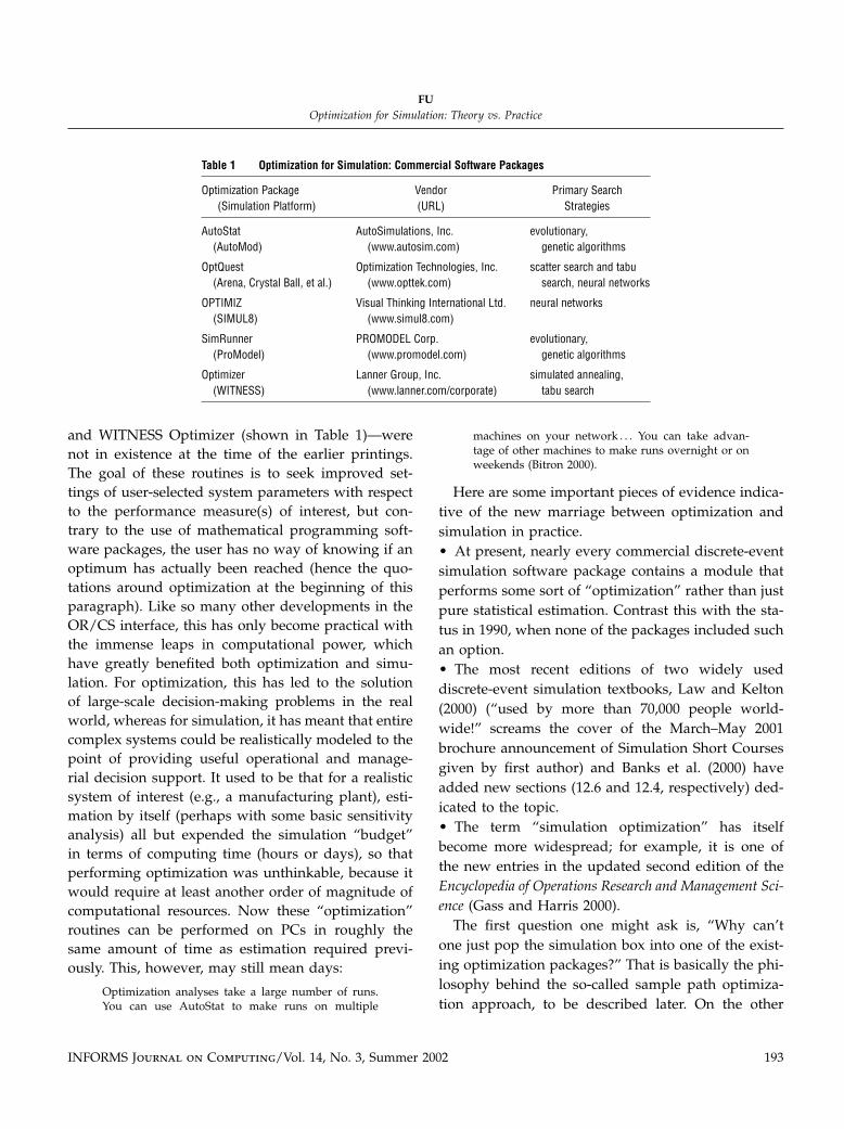
for the quotes will be explained shortly) have promi-nently worked their way into simulation packages.That this is a fairly recent development is revealedby the fact that all of the software routines for per-forming simulation optimization listed in the cur-rent edition of Law and Kelton (2000, p. 664, Table12.11)—AutoStat, OptQuest, OPTIMIZ, SimRunner,

INFORMS Journal on Computing © 2002 INFORMSVol. 14, No. 3, Summer 2002 pp. 192–215

0899-1499/02/1403/0192$5.001526-5528 electronic ISSN

FUOptimization for Simulation: Theory vs. Practice

Table 1 Optimization for Simulation: Commercial Software Packages

Optimization Package Vendor Primary Search(Simulation Platform) (URL) Strategies

AutoStat AutoSimulations, Inc. evolutionary,(AutoMod) (www.autosim.com) genetic algorithms

OptQuest Optimization Technologies, Inc. scatter search and tabu(Arena, Crystal Ball, et al.) (www.opttek.com) search, neural networks

OPTIMIZ Visual Thinking International Ltd. neural networks(SIMUL8) (www.simul8.com)

SimRunner PROMODEL Corp. evolutionary,(ProModel) (www.promodel.com) genetic algorithms

Optimizer Lanner Group, Inc. simulated annealing,(WITNESS) (www.lanner.com/corporate) tabu search

and WITNESS Optimizer (shown in Table 1)—werenot in existence at the time of the earlier printings.The goal of these routines is to seek improved set-tings of user-selected system parameters with respectto the performance measure(s) of interest, but con-trary to the use of mathematical programming soft-ware packages, the user has no way of knowing if anoptimum has actually been reached (hence the quo-tations around optimization at the beginning of thisparagraph). Like so many other developments in theOR/CS interface, this has only become practical withthe immense leaps in computational power, whichhave greatly benefited both optimization and simu-lation. For optimization, this has led to the solutionof large-scale decision-making problems in the realworld, whereas for simulation, it has meant that entirecomplex systems could be realistically modeled to thepoint of providing useful operational and manage-rial decision support. It used to be that for a realisticsystem of interest (e.g., a manufacturing plant), esti-mation by itself (perhaps with some basic sensitivityanalysis) all but expended the simulation “budget”in terms of computing time (hours or days), so thatperforming optimization was unthinkable, because itwould require at least another order of magnitude ofcomputational resources. Now these “optimization”routines can be performed on PCs in roughly thesame amount of time as estimation required previ-ously. This, however, may still mean days:

Optimization analyses take a large number of runs.You can use AutoStat to make runs on multiple

machines on your network � � � You can take advan-tage of other machines to make runs overnight or onweekends (Bitron 2000).

Here are some important pieces of evidence indica-tive of the new marriage between optimization andsimulation in practice.• At present, nearly every commercial discrete-eventsimulation software package contains a module thatperforms some sort of “optimization” rather than justpure statistical estimation. Contrast this with the sta-tus in 1990, when none of the packages included suchan option.• The most recent editions of two widely useddiscrete-event simulation textbooks, Law and Kelton(2000) (“used by more than 70,000 people world-wide!” screams the cover of the March–May 2001brochure announcement of Simulation Short Coursesgiven by first author) and Banks et al. (2000) haveadded new sections (12.6 and 12.4, respectively) ded-icated to the topic.• The term “simulation optimization” has itselfbecome more widespread; for example, it is one ofthe new entries in the updated second edition of theEncyclopedia of Operations Research and Management Sci-ence (Gass and Harris 2000).The first question one might ask is, “Why can’t

one just pop the simulation box into one of the exist-ing optimization packages?” That is basically the phi-losophy behind the so-called sample path optimiza-tion approach, to be described later. On the other

INFORMS Journal on Computing/Vol. 14, No. 3, Summer 2002 193


hand, here is the counter view of one of the softwareproviders (www.opttek.com, November 2000):

The most commonly used optimization procedures—linear programming, nonlinear programming and(mixed) integer programming—require an explicitmathematical formulation. Such a formulation is gen-erally impossible for problems where simulation isrelevant, which are characteristically the types ofproblems that arise in practical applications.

The term “simulation” will henceforth be short-hand for stochastic discrete-event simulation, mean-ing that the random nature of the system will beimplicitly understood and the underlying models arediscrete-event systems such as queueing networks.In fact, it is the stochastic nature that is key in allof the discussion, and one central thesis of this arti-cle is that the currently implemented optimizationalgorithms do not adequately address this charac-teristic. The focus on discrete-event simulation hastwo rationales: It is the primary domain of opera-tions researchers in stochastic simulation (as opposedto, for example, stochastic differential equations inthe fields of computational finance or stochastic con-trol), and it is where optimization and simulationhave come together most prominently in commercialsoftware. The primary application areas are manufac-turing, computer and communications networks, andbusiness processes.The selection of the title of this article, “Optimiza-

tion for Simulation,” was made quite deliberately. Thetwo most recent comprehensive survey articles onthe subject, Fu (1994) and Andradóttir (1998), aretitled “Optimization via Simulation” and “SimulationOptimization,” respectively, reflecting the two termsmost commonly used in the field (see also Swisheret al. 2001). These two titles more accurately reflectthe state of the art in the research literature, whereasthe purpose of this article is to explore the linkages(and lack thereof) with the practice of discrete-eventsimulation. In that sense, it is not an equal partnershipbut a subservient one, in which the optimization rou-tine is an add-on to the underlying simulation engine,as depicted in Figure 1. In contrast, one can view therecent developments in stochastic programming asthe converse, simulation for optimization, as depictedin Figure 2, where Monte Carlo simulation is the add-on used to generate scenarios for math programming

Figure 1 Optimization for Simulation: Commercial Software

formulations from a relatively small underlying set ofpossible realizations. One of the primary applicationareas of this approach is financial engineering, e.g.,portfolio management.In the literature, there is a wide variety of terms

used in referring to the inputs and outputs of asimulation optimization problem. Inputs are called(controllable) parameter settings, values, variables,(proposed) solutions, designs, configurations, or fac-tors (in design of experiments terminology). Out-puts are called performance measures, criteria, orresponses (in design of experiments terminology).Some of the outputs are used to form an objec-tive function, and there is a constraint set on theinputs. Following deterministic optimization common

Figure 2 Simulation for Optimization: Stochastic Programming

194 INFORMS Journal on Computing/Vol. 14, No. 3, Summer 2002


usage, we will use the terms “variables” and “objec-tive function” in this article, with the latter comprisedof performance measures estimated from simulation(consistent with discrete-event simulation commonusage). A particular setting of the variables will becalled either a “configuration” or a “design.”The general setting of this article is to find a

configuration or design that minimizes the objectivefunction:

min�∈�

J ��= E�L�� (1)

where � ∈� represents the (vector of) input variables,J �� is the objective function, � represents a sam-ple path (simulation replication), and L is the sam-ple performance measure. We will use J to representan estimate for J ��, e.g., L�� would provide onesuch estimator that is unbiased. The constraint set �may be either explicitly given or implicitly defined.For simplicity in exposition, we assume throughoutthat the minimum exists and is finite, e.g., � is com-pact or finite, as opposed to using “inf” and allowingan infinite value. Throughout, J will be scalar andan expectation; multiple performance measures canbe handled simply by assigning appropriate weightsand combining to form a single objective function,though this may not always be desirable or practi-cal (but very little has been done on multi-responsesimulation optimization). Note that probabilities canbe handled as expectations of indicator functions, butthat quantiles (e.g., the median) and measures such as“most likely to be the best” (e.g., mode) are excludedby this form of performance measure. Most of thecommercial software packages also allow the prac-tically useful extension of the setting in (1) to thatof including explicit inequality constraints on out-put performance measures (as opposed to the indirectway of incorporating them into the objective functionby way of a penalty function or Lagrange multipliers).The categories of inputs are generally divided into

two types: qualitative and quantitative. The formerare characterized by not having a natural ordering(either partial or full). The latter are then furtherdivided into two distinct domains of discrete andcontinuous variables, analogous to deterministic opti-mization, where the approaches to these types ofproblems can also be quite different.

Real-World Example: Call Center Designand OperationsCustomer Relationship Management (CRM) is cur-rently one of the hottest topics (and buzzwords)in business management (ranked #1 in technologytrends for 2001 by M. Vizard, the Editor in Chief ofInfo World, p. 59 of January 8, 2001 issue, “Top 10technology trends for 2001 all ask one thing: Are youexperienced?”).

This isn’t just about providing adequate supportwhen a customer needs help, but rather about offer-ing the customer an overall relationship with the com-pany that’s valuable, compelling and unavailable any-where else � � � (The Industry Standard, “You and YourCustomer,” Nov. 6, 2000, pp. 154–155.)

For example, IBM has an “eCare” program, with theobjective of delighting the customer, which translatesinto personalizing information and support on theWeb. One of Oracle’s major advertising campaignsin 2001 promises “global CRM in 90 days.” Ama-zon.com has a Vice-President of CRM, though theacronym has a little different twist on it: Customer-Relationship Magic. The technology underlying CRMinvolves data warehousing and data mining, but formany businesses, the key CRM storefront is the callcenter that handles customer orders (for products orservices), inquiries, requests, and complaints. “Cus-tomer support, in fact, is one of the most commonways businesses can put their CRM strategy to work”(ibid.). Far from being just a staid telephone switch-board, the state of the art integrates traditional calloperations with both automated response systems(computer account access) and Internet (Web-based)services and is often spread over multiple geographi-cally separate sites. For this reason, the term “call cen-ter” is rapidly being supplanted by the more dynamicand all-encompassing appellation “contact center” toreflect more accurately the evolving nature of thediverse activities being handled.Most of these centers now handle multiple sources

of jobs (“multichannel contact”), e.g., voice, e-mail,fax, interactive Web, which require different levels ofoperator (call agent) training, as well as different pri-orities, as voice almost always preempts any of theother contact types (except possibly interactive Web).There are also different types of jobs according to the



service required, e.g., an address change versus check-ing account balance versus a more involved transac-tion or request; hence, the proliferation of bewilder-ing menu choices on the phone. Furthermore, becauseof individual customer segmentation, there are differ-ent classes of customers in terms of priority levels.In particular, many call centers have become quitesophisticated in their routing of incoming calls by dif-ferentiating between preferred, ordinary, and “unde-sirable” (those that actually cost more to serve thantheir value added) customers. The easiest way toimplement this is to give special telephone numbersto select customers. Most airline frequent flier pro-grams do this, so on Continental Airlines, I am spe-cial and pampered, but on US Airways I am ordinary.Other call center systems request an account num-ber and use this as part of their routing algorithm.When I punch in my account number to CharlesSchwab’s Signature Service line, I receive an opera-tor almost immediately. “Based on a customer’s code,call centers route customers to different queues. Bigspenders are whisked to high-level problem solvers.Others may never speak to a live person at all � � �”(Business Week Cover Story, pp. 118–128, October 23,2000) “Walker Digital, the research lab run by Price-line founder Jay S. Walker, has patented a ‘value-based queuing’ of phone calls that allows companiesto prioritize calls according to what each person willpay. As Walker Digital CEO Vikas Kapoor argues, cus-tomers can say: ‘I don’t want to wait in line—I’ll payto reduce my wait time’ ” (ibid.). What this means isthat call-routing algorithms (implemented as rules inthe automatic call distributor—ACD) are now a keyintegral part of providing the right level of customerservice to the right customers at the right time.Designing and operating such a call center

(the CTI—computer telephony integration—strategy)entails many stochastic optimization problems thatrequire selection of optimal settings of certain vari-ables, which may include quantitative (e.g., numberof operators at each skill level and for each particularclass of customer, number and types of telecommu-nications devices) and qualitative (e.g., what routingalgorithm and type of queue discipline to use: FCFS,priority to elite customers, or something else) dimen-sions. The objective function will consist of metrics

associated with both customers and agents. For exam-ple, there are cost components associated with servicelevel performance measures such as waiting times(most commonly the mean or the probability of wait-ing more than a certain amount of time, possiblyweighted by class type) and operational costs asso-ciated with agent wages and network usage (trunkutilization). Abandonment rates of waiting customers,percentage of blocked calls (those customers thatreceive a busy signal), and agent utilization are otherfactors that are considered. Clearly, there is a trade-offthat must be made between customer service levelsand the cost of providing service. As in any optimiza-tion problem, this could be expressed with a singleobjective function, e.g., minimize costs subject to anumber of different constraints, such as pre-specifiedcustomer service levels for each class of customer(lower bound for preferred customers, perhaps upperbound for undesirable ones?).

Toy Example: Single-Server QueueThe most studied OR model in the illustrious his-tory of queueing theory still necessitates simulationin many cases. Consider a first-come, first-served,single-class, single-server queue with unlimited wait-ing room, such that customer service times are drawnindependently from the same probability distribution(single class of customers) and the controllable vari-able is the speed of the server. Let � denote the meanservice time of the server (so 1/� corresponds to theserver speed). Then one well-studied optimizationproblem uses the following objective function:

J ��= E�W��+ c/� (2)

where W is the steady-state time spent in the systemand c is the cost factor for the server speed. In otherwords, a higher-skilled worker costs more. Since W isincreasing in �, the objective function clearly quanti-fies the trade-off between customer service level andcost of providing service. This could be viewed as thesimplest possible case of the call center design prob-lem, where there is a single operator whose skill levelmust be selected. Simulation of this system requiresspecification of the arrival process and the servicetime distribution. In addition to its honored place inqueueing theory, this model is often the first system



used in textbooks to illustrate discrete-event simu-lation (e.g., Law and Kelton 2000). For the simplestM/M/1 queue in steady state, this problem is ana-lytically tractable, and thus has served as an easytest case for optimization procedures, especially thosebased on stochastic approximation.

Another Academic Example: �s S� InventoryControl SystemThis is another well-known OR model from inven-tory theory, in which the two parameters to be opti-mized, s and S, correspond to the re-order leveland order-up-to level, respectively. When the inven-tory level falls below s, an order is placed for anamount that would bring the current level back upto S. Optimization is generally carried out by mini-mizing a total discounted or average cost function—consisting of ordering, holding, and backlogging orlost sales components—or just ordering and hold-ing costs but subject to a service level constraint.In research papers on simulation optimization, thisexample is nice, because it is the simplest multi-dimensional problem (as opposed to the previousscalar one), and being in two dimensions, it has anice graphical representation in search procedures(see Section 4). Thus, it has been used as a test casefor nearly all the procedures in the research literaturediscussed in Section 4, i.e., stochastic approximation,sequential response surface methodology, retrospec-tive optimization (an early incarnation of sample pathoptimization), statistical ranking and selection, andmultiple comparisons.To attack the generic problem posed by (1), the five

packages listed in the opening paragraph use meta-heuristics from combinatorial optimization based onevolution strategies such as genetic algorithms, tabusearch, and scatter search (see Glover et al. 1999),with some adaptation of other techniques taken fromthe deterministic optimization literature, e.g., neu-ral networks and simulated annealing (even thoughthe latter is probabilistic in nature, it has been pri-marily applied to deterministic problems). On theother hand, the research literature in simulation opti-mization (refer to Andradóttir 1998 or Fu 1994) isdominated by continuous-variable stochastic approx-imation methods and random search methods for

discrete-variable problems, which consist primarilyof search strategies iterating a single point, versusthe group or family of points adopted by the meta-heuristics above. The continuous-variable algorithmsare predominantly based on local gradient search.Thus, in terms of software implementation, the

available routines are based on approaches outside ofthe simulation research literature. Indeed, other thanin the Winter Simulation Conference Proceedings, onewould be hard-pressed to find published examplesof metaheuristics represented in archival journals onsimulation. “Why is this the case?” you might ask.There appear to be two major barriers: Either the algo-rithms that are implemented are not provably conver-gent, or the use of simulation is secondary. In the lat-ter case, it seems more appropriate that the algorithmbe published in the Journal of Heuristics—with roots inthe combinatorial optimization community—than inthe ACM Transactions on Modeling and Computer Sim-ulation, the most highly respected OR journal dedi-cated to stochastic simulation, whose founding editoris from a computer science department but whose edi-torial board is dominated by OR researchers in thesimulation community.“What will the remainder of this article try to

accomplish?” you might naturally ask at this point.(Or, “Why should I read any further, since I alreadyhave the main idea?”) It will attempt to do the fol-lowing:• Explain why optimization for simulation shouldnot merely consist of deterministic algorithms appliedto a black box that happens to be a simulation model.• Provide a representative, but by no means exhaus-tive, high-level description of the algorithms and the-oretical convergence results in the simulation opti-mization literature and of the relevant related resultsfrom the stochastic optimization literature.• Contrast with the routines that are found incommercial discrete-event simulation software bydescribing the general search strategies of two pack-ages and delving into the specific user-specifiedparameters and provided outputs for one of them.• Touch upon research directions that are importantor promising, in the author’s humble opinion, andspeculate on the future of optimization for simulation,both in theory and in practice.



The remainder of this article is organized as fol-lows. Section 2 expatiates further on those featuresthat make optimization for simulation more than sim-ply a straightforward implementation of determinis-tic algorithms. It includes a summary of challengescommon to both research and practice, along withkey issues that separate the two. A (very) brief tuto-rial on simulation output analysis and probabilisticconvergence modes is also provided as backgroundor review material. Section 3 surveys the researchapproaches for simulation optimization and providesa flavor of the theoretical results in the literature.Section 4 contrasts research with practice by describ-ing two commercial software routines that imple-ment optimization for simulation. Future directionsin research and in practice are then discussed inSection 5. The article concludes with a brief sectionon sources for probing further.

2. What Makes SimulationOptimization Different?

As alluded to earlier, what makes simulation opti-mization doubly difficult on top of the ordinary deter-ministic optimization setting is its stochastic nature.A nice summary of this key difficulty is provided byBanks et al. (2000, p. 488):

Even when there is no uncertainty, optimization canbe very difficult if the number of design variablesis large, the problem contains a diverse collectionof design variable types, and little is known aboutthe structure of the performance function. Optimiza-tion via simulation adds an additional complicationbecause the performance of a particular design cannotbe evaluated exactly, but instead must be estimated.Because we have estimates, it may not be possibleto conclusively determine if one design is better thananother, frustrating optimization algorithms that tryto move in improving directions. In principle, one caneliminate this complication by making so many repli-cations, or such long runs, at each design point thatthe performance estimate has essentially no variance.In practice, this could mean that very few alternativedesigns will be explored due to the time required tosimulate each one.

In the problem setting of (1), the usual goals of opti-mization can be stated succinctly as follows:(a) Finding argmin�∈� J ��

(or at least one element, if the argmin is a set, i.e., theproblem has multiple optima).

(b) Returning min�∈� J ��.For example, think of the practical problem of find-ing the quickest route to work each morning. Thenthe corresponding questions to be answered are: (a)Which roads should I take? (b) How long will it take?In deterministic optimization, all the emphasis is on(a), because (b) is trivial once (a) is accomplished, i.e.,if �∗ ∈ argmin J ��, then min�∈� J �� = J ��∗�. In otherwords, one does not generally distinguish betweenthe two as being separate problems in the deter-ministic setting. In a stochastic (and real-life) setting,however, one must change (b) to the following: esti-mating min�∈� J ��. In fact, sometimes it is only (a)that is of ultimate (or primary) interest, and J is sim-ply the means to the end. This is usually the case inthe going-to-work example, since, unless you are cut-ting it very close to meet a tight scheduled appoint-ment, you are probably more interested in finding thequickest route than in precisely estimating the actualtotal travel time. Furthermore, I “know” that in gen-eral taking the beltway is much quicker than takingall local roads, but I have only a rough estimate ofthe time it takes for the portion of time spent on thehighway (10 to 15 minutes), and very little idea as tohow long a totally local route would take (at least anhour?). Here are some other examples:• Preventive Maintenance: Finding an optimal (or agood) policy is most likely the goal, with the cost esti-mates often only a rough gauge of various operationalaspects.• Manufacturing Plant Design: Selection of the bestdesign is the primary goal, rather than the cost (orprofit) estimate.• Derivatives Pricing: Options with early exerciseopportunities require the determination of an optimalpolicy in order to find the price; however, in this case,the situation is reversed, as it is the estimated pricethat is paramount and not the policy itself.The actual process of optimization can be divided

into two parts:(I) Generating candidate solutions.(II) Evaluating solutions.In optimization for simulation, the perspective of

practice in terms of coming up with algorithms is toconcentrate on the first step, just as in the determin-istic case, treating the simulation model essentially



Figure 3 Optimization for Simulation: Practice Perspective

as just another function generator with some statis-tical analysis, as shown in Figure 3. In optimizationfor simulation, however, most of the computation isexpended in estimating J �� for values of � in thesearch, a reversal of the deterministic setting, wherethe search is the primary computational burden. Thus,the commercial software view shown in Figure 1,where optimization is viewed as simply another sub-routine add-on, also reflects the computational bal-ance between the two functions. A major determinantof the computational cost for a simulation optimiza-tion algorithm is the number of simulation replica-tions used to estimate J �� for each �. For example,there is no reason a priori to assume that the numberof replications should be the same for all values of �nor the same for each iteration in the search process.In sum, a key feature that is not a factor in deter-ministic settings is the trade-off between the amountof computational effort needed to estimate the per-formance at a particular solution versus the effortin finding improved solution points (or families). Arelated (motivating?) point is that the focus shouldtherefore be on comparing relative performance insteadof estimating absolute performance, i.e., order is theessential goal during the search process. In contrast,when there is an absence of randomness, calculatingabsolute performance is essentially indistinguishablefrom comparing relative performance.To summarize, the process in a stochastic setting

should be modified as follows (shown in Figure 4):(I) Iterative but Integrated: Searching and Compar-

ing; finding �∗.

Figure 4 Optimization for Simulation: Future Needs

(II) Final: Estimating the optimal value of objectivefunction J ��∗�.As noted earlier, step (II) may or may not be the ulti-mate objective.Because, in the deterministic setting, evaluating and

comparing are considered essentially the same step,currently implemented simulation optimization rou-tines do not really address (much less exploit) thenotion of ordinal comparisons. To reiterate this crucialpoint:

It is generally easier to compare solutions and findrelative ordering among them than it is to estimatethem precisely.

This is the main basis of the so-called ordinal opti-mization approach, where the goal is approximateorder, rather than precise values. As an aside, thisis also the philosophy behind the analytic hierarchyprocess (AHP), where relative weights are consideredkey.Banks et al. (2000, pp. 488–489) break down the

approaches toward optimization via simulation intofour categories:• guarantee asymptotic convergence to the optimum(generally for continuous-valued parameters);• guarantee optimality under deterministic counter-part (i.e., if there were no statistical error or sam-pling variability; generally based on mathematicalprogramming formulations);• guarantee a prespecified probability of correctselection (generally from a prespecified set of alterna-tives);



• robust heuristics (generally based on combinatorialsearch algorithms that use an evolutionary approach,e.g., genetic algorithms).Going down the list, there is a transition from com-plete confidence in optimality, albeit in an unrealiz-able context, to workable solutions that apply in prac-tical settings. This mirrors the tug of war betweenresearch and practice that involves a dueling betweenapproaches that provide quick rough-and-ready solu-tions with no performance guarantees (based onheuristics, with no statistical analysis whatsoever)versus the more rigorous mathematical approachesdominating the academic literature that either guar-antee convergence or probability of correct selection.Here is an illustration of each of these using the toy

example, where the objective is to select the skill level(speed) of the call center operator.• The operator skill level is variable over a rangeof values, which can be either continuous (e.g., forstochastic approximation algorithms) or discrete (e.g.,using random search). The algorithm will find anoptimum (single value) for sure (100% confidence) ifthe algorithm is run “long enough.”• Again, the operator skill level is variable over acontinuous range of values. The algorithm returns anoptimum (single value) under the case where each sim-ulation (versus the algorithm itself, in the previouscase) is run “long enough.”• Reduce the problem to a fixed (relatively small)finite number of operator skill levels from which tochoose. The algorithm will select a skill level withobjective function value within � of the best at a�1−�)100% confidence level, where the confidencelevel is generally a lower bound.• The operator skill level is variable over a range ofvalues, which could be discrete or continuous. Theroutine will return the best found values from a fam-ily and provide an estimate of improvement from thebeginning of the search.Parallel results could be described for the inventoryexample, corresponding to modeling demand andinventory quantities as continuous valued (e.g., gal-lons of oil), or discrete valued (e.g., number of books).

2.1. Research and Practice: Key IssuesIt can be argued that both research and practice haveadapted approaches from deterministic optimization,

Table 2 Approaches from Deterministic Optimization

Approach Key Features

Gradient search Move locally in most promising direction,according to gradient

Random search Move randomly to new point,no information used in search

Simulated annealing Sometimes move in locally worse directions,to avoid being trapped in local extrema

Genetic algorithms Population based, generates new members usingand scatter search (local) operations on attributes of

current membersTabu search Use memory (search history) to avoid tabu movesNeural networks (Nonlinear) function approximationMath programming Powerful arsenal of rigorously tested software

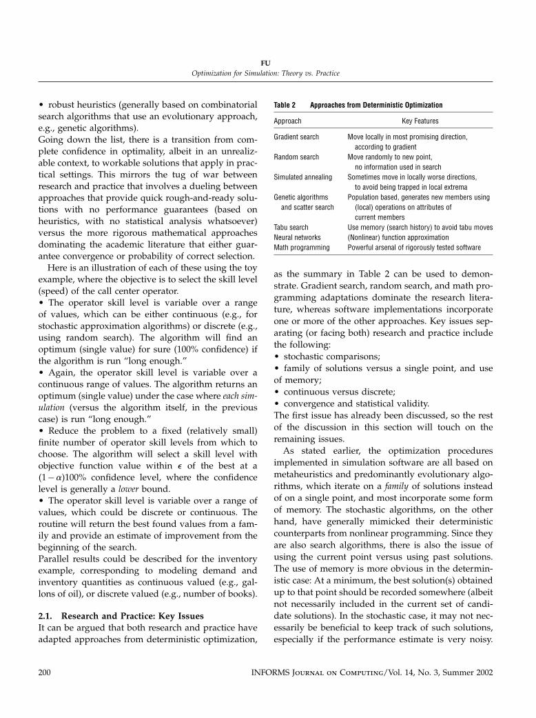
as the summary in Table 2 can be used to demon-strate. Gradient search, random search, and math pro-gramming adaptations dominate the research litera-ture, whereas software implementations incorporateone or more of the other approaches. Key issues sep-arating (or facing both) research and practice includethe following:• stochastic comparisons;• family of solutions versus a single point, and useof memory;• continuous versus discrete;• convergence and statistical validity.The first issue has already been discussed, so the restof the discussion in this section will touch on theremaining issues.As stated earlier, the optimization procedures

implemented in simulation software are all based onmetaheuristics and predominantly evolutionary algo-rithms, which iterate on a family of solutions insteadof on a single point, and most incorporate some formof memory. The stochastic algorithms, on the otherhand, have generally mimicked their deterministiccounterparts from nonlinear programming. Since theyare also search algorithms, there is also the issue ofusing the current point versus using past solutions.The use of memory is more obvious in the determin-istic case: At a minimum, the best solution(s) obtainedup to that point should be recorded somewhere (albeitnot necessarily included in the current set of candi-date solutions). In the stochastic case, it may not nec-essarily be beneficial to keep track of such solutions,especially if the performance estimate is very noisy.



The use of long runs or many replications clearlyreduces the noise and brings the stochastic settingcloser to the deterministic domain. Random searchalgorithms often count the number of visits to promis-ing configurations.In addition to the use of a family of points, the algo-

rithms implemented in software are primarily basedon discrete search strategies, and, as such, definetheir own neighborhood structure, not assuming (orexploiting), though possibly inheriting, order inherentin the variable space, e.g., on the real line. Exploit-ing such order is clearly used in continuous opti-mization algorithms. The generality gained by themetaheuristic approaches may come at the cost ofefficiency for problem settings with structure. Forexample, discrete-event system models clearly exhibitcertain characteristics that may be amenable to moreefficient search such as algorithms based on gradientinformation.A useful notion defined in statistical ranking and

selection procedures is the concept of correct selectionand the computation, or bounding, of its probabil-ity. Correct selection refers to choosing a configura-tion of the input variables that optimizes the objectivefunction. Many iterative search algorithms have anasymptotic probability of correct selection of 1. Rank-ing and selection procedures introduce the concept ofan indifference zone, say �, which provides a measureof closeness that the decision maker tolerates awayfrom absolute optimality. This is analogous to the goodenough sets defined in ordinal optimization. In thiscase, correct selection corresponds to either choosing aconfiguration with the optimum value of the objectivefunction or a configuration whose objective functionvalue is within � of the optimal value. The usual state-ment of performance guarantees for these proceduresis to specify a lower bound on the probability of cor-rect selection, in the form of a �1−��100% confidencelevel.We revisit the issue of convergence and statistical

validity in more detail now, in preparation for thedescription of these procedures in the next section. Inwords, the algorithms in the research literature pro-vide the following:• Stochastic Optimization Procedures (e.g., stochas-tic approximation, random search, sample path

optimization): convergence to a true optimum (butpossibly only local) under some probabilistic metric.• Ranking and Selection Procedures: selection of abest solution (or set of best solutions) at some pre-specified statistical level.Typical examples of research results take the follow-ing form:• Stochastic Optimization Procedures:

�n −→ �∗ w.p. 1

which is also known as almost sure (a.s.) convergence.Other common forms of convergence include con-vergence in probability (measure) and convergencein distribution (also known as weak convergence, aterm that confusingly enough does not correspond tothe weak law of large numbers, which instead is aconvergence-in-probability result). Defining these rig-orously is beyond the scope of this article (refer toWolff 1989, Sec.1–16, for example). In the next section,we review some of the modes via some well-knownexamples.• Ranking and Selection Procedures: Probability thatthe selected � is within � of the best is at least �1−��.In contrast, very little in the way of theoretical con-vergence results exists for the metaheuristics (refer toTable 2) in the deterministic framework; none that theauthor is aware of in the stochastic environment.

2.2. A Brief TutorialThis section reviews rudimentary material on prob-abilistic convergence modes and simulation outputanalysis at the minimum level required for readingthis article.

2.2.1. A Very Basic Primer on Simulation OutputAnalysis. Simulationists can (and should) skip thissubsection, which diverges to speak to those with lit-tle simulation background or those on the determin-istic side who did not listen very carefully to theirsimulation professor. The reader is referred to Lawand Kelton (2000) or Banks et al. (2000) for furtherin-depth coverage.The message is this basic tenet of statistical output

analysis:

Simulation estimates should be accompanied withsome indication of precision!



The usual textbook instruction is to provide confi-dence intervals, e.g., a 95% confidence interval formean response time is 97 seconds ± 5 seconds. Aless strict, implicit means of providing a rough indica-tion of precision is the reporting of significant digits.Under this convention, if the single number 97 sec-onds is presented (e.g., to upper-level management,who would just as soon not see the ± 5 seconds),the presumption should be that the precision is some-where on the order of 1 to 10 seconds. In other words,do not report the number 97.395 seconds alone (97.395seconds ± 5.321 seconds is acceptable, but not as pre-ferred as either 97 ± 5 or 97 ± 5.3) unless the pre-cision extends to the third decimal place, because itis extremely misleading! Unfortunately, the softwaremakes reporting large number of decimal places tooeasy for the user.For estimating a single performance measure, a

good rough measure of precision is provided by thestandard error

s/√n

where s is the sample standard deviation and n isthe number of simulation replications. An approxi-mate 95% confidence interval is constructed by tak-ing two standard errors on both sides of the sam-ple mean. Such an interval is not appropriate whenthe estimated performance is heavily skewed (e.g., forrare-event measures).For comparing performances of various designs,

one uses pairwise comparisons. Individual measuresof precision on each pair can be found and combinedwith the Bonferroni inequality to get an overall con-fidence level lower bound, or a simultaneous confi-dence level can be obtained that coordinates all ofthe pairs.Consider just two systems. The most easily applied

method to compare them is to use the paired-t con-fidence interval to check the direction of the sign(technically, checking the hypothesis of whether ornot the difference in the means is zero). If the confi-dence interval contains zero, then, statistically speak-ing, there is no difference. In fact, it is almost alwaysthe case in practice that the analyst believes that thereis a difference, and it is the direction that is to beinferred. In order to make this inference, the ana-lyst desires a confidence interval that doesn’t contain

zero. To achieve this clearly depends on the followingfactors:• actual difference in the means;• variance of each of the estimators;• covariance between the estimators.If an efficient direct estimator for the difference couldbe found, that would be ideal. In practice, the analysttakes the individual estimators and forms an estima-tor for the difference by taking the difference betweenthe two in the obvious manner. Inducing positive cor-relation will reduce the size of the confidence interval,since

Var�X−Y � = VarX+VarY −2Cov�XY �

< VarX+VarY if Cov�XY � > 0�

This is the main idea behind the method of commonrandom numbers, but it is also the basis for otherschemes to effectively couple the individual underly-ing stochastic processes.

2.2.2. Review of Convergence Modes. By wayof three well-known examples in classical statisticsand one less widely known result, we compare vari-ous forms of convergence that are found in researchresults on stochastic optimization. Let Xn denote thesample mean over n i.i.d. samples �Xi� with com-mon mean � and variance �2, with N��2� denot-ing the normal distribution with mean � and variance�2.• Strong Law of Large Numbers (SLLN)

Xn −→ � w.p. 1.

• Weak Law of Large Numbers (WLLN)

Xn −→ � in probability�

• Central Limit Theorem (CLT)

Xn −→ N��2/n� in distribution�

• Large Deviations Type of Result

P�Xn ∈ ��− ��+ ��−→ e−nf ��

e.g., if Xi ∼ N��2�, then f �x�= �x/��2/2.



All of these results make statements about the con-vergence of the sample mean to the true mean for alarge enough number of samples. Although the CLThas a weaker type of convergence than the two lawsof large numbers, it is a stronger result, because itprovides the actual asymptotic distribution, while stillguaranteeing convergence to the mean, since the vari-ance �2/n goes to 0 as n goes to infinity. This varianceterm in fact provides an estimate of the precision ordistance of the sample mean from the true mean for alarge number of samples. In other words, it providesthe well-known O�1/

√n� convergence rate for Monte

Carlo simulation.The last result makes a probability statement on the

deviation of the sample mean from the true mean. Asthe number of samples gets larger, the probability ofa large deviation from the true mean vanishes expo-nentially fast. Note that although this also provides aconvergence rate, it differs from the CLT result in thatthe rate is with respect to a probability rather than forestimation per se. In a very crude sense, one can viewthis as refining the WLLN result with a convergencerate, whereas the CLT result provides a convergencerate for the SLLN version.Picking the arg min can be associated with the last

result, whereas actually estimating the optimal valuehas a convergence rate governed by the CLT result.Hence, finding the optimum may result in exponen-tial convergence, whereas estimating the correspond-ing value is constrained by the standard canonicalinverse square root rate of Monte Carlo simulationreferred to above. Clearly, this distinction is absent indeterministic optimization, but the currently imple-mented optimization routines completely ignore thisconcept!

3. Simulation OptimizationResearch

The most relevant topics in the research literatureinclude the following:• ranking and selection, multiple comparison proce-dures, and ordinal optimization;• stochastic approximation (gradient-basedapproaches);• (sequential) response surface methodology;

• random search;• sample path optimization (also known as stochasticcounterpart).This section includes a summary of the main ideas

and a brief survey of some of the research results.

3.1. Ranking and Selectionand Ordinal Optimization

We begin with relevant work that focuses on thecomparison theme rather than the search algorithms,because this is a central issue in optimization forsimulation that practice has not fully addressed (orexploited). Although usually listed separately fromsimulation optimization in simulation textbooks orhandbook chapters (e.g., Law and Kelton 2000, Bankset al. 2000, Banks 1998), ideas from the ranking andselection (R&S) literature (taken here to include mul-tiple comparison procedures), which uses statisticalanalysis to determine ordering, have important impli-cations for optimization. The primary feature differ-entiating R&S procedures (see, for example, Golds-man and Nelson 1998) from optimization proceduresis that the R&S procedures evaluate exhaustively allmembers from a given (fixed and finite) set of alter-natives, whereas optimization procedures attemptto search efficiently through the given set (possiblyimplicitly defined by constraints) to find improvingsolutions, because exhaustive search is impractical orimpossible (e.g., if the set is unbounded or uncount-able). As a result, R&S procedures focus on the com-parison aspect, which is a statistical problem uniqueto the stochastic setting. Clearly, statistics (and prob-ability theory) must also come into play if any con-vergence results are to be rigorously established forthe search algorithms. Thus, these procedures shouldplay a major role in optimization for simulation.Two important concepts in the methodology have to

do with user specification of the following levels:• an indifference zone (level of precision);• a confidence level (probability of correct selection).At a certain level, these are analogous to confidenceintervals in estimation, except that both have to bespecified here, whereas in estimation the analyst spec-ifies either a precision or a confidence level, andthe other follows. To illustrate for the single-server



queue example, an estimation goal might be to esti-mate mean response time within a precision of plusor minus 10 seconds, or with a 95% confidence level,whereas the selection criterion might be to select anoperator that results in an average daily operatingcost within $10 of optimality at a 95% confidencelevel.The key idea behind the so-called ordinal optimiza-

tion approach (Ho et al. 1992, 2000) is that it is mucheasier to estimate approximate relative order than pre-cise (absolute) value. In addition, there is goal soften-ing; instead of looking for the best, one settles for asolution that is good enough, which would have to bestatistically defined. The former has a common goalwith multiple comparison procedures, while the lat-ter is clearly similar in spirit to the indifference zoneapproach of R&S procedures.

3.1.1. Exponential Convergence of Ordinal Com-parisons. The term output analysis in stochastic sim-ulation refers to the statistical analysis of simulationoutput over a set of simulation replications (sam-ples) or one long simulation, with the most basicresult being the O�1/

√n� convergence rate of Monte

Carlo estimation. However, comparisons often exhibitasymptotic convergence rates that are exponential.

Example: Two Configurations. Consider the sim-ple “optimization” problem of determining which oftwo configurations has the smallest mean of the out-put performance measure, where only samples areavailable to estimate the mean. For simplicity, theperformance measures are taken to be normally dis-tributed (unbeknownst to the optimizer analyst):

� = ��a �b� L��a�∼ N�01/4�L��b�∼ N�d1/4� d > 0�

In this case, the optimal configuration is �a, sinceJ ��a� = E�L��a�� = 0 < d = E�L��b�� = J ��b�. With justtwo configurations, the optimization problem can bereduced to simply determining whether the differ-ence of the means is positive or negative. To this end,define the difference random variable:

X = L��b�−L��a��

Assuming that n independent pairs of samples aretaken from each configuration, let Xi denote the ithsuch sample, following distribution N�d1/2�. Let �denote the indifference amount. Then one approachwould be to estimate each of the two configurationsindependently until two standard errors for each esti-mate is less than �. After that, the two means arecompared to decide which is smaller.For illustrative purposes, consider a numerical

example where � = 0�1. Then it would take approxi-mately 100 samples to achieve the desired precisionfor each configuration, regardless of the value of d.What about the probability of correct selection? Wehave said that the complement of this probabilitydecreases to zero exponentially. However, the rate ofthis decay depends on the value of d. For this sim-ple example, these probabilities are easily calculatedusing the standard normal cumulative distributionvalues. Figure 5 illustrates the convergence rate of thisprobability of correct selection for difference valuesof d (0.01, 0.1, 0.2, 0.3, 1.0), with the 1/

√n convergence

rate also included for comparison. Thus, to achieveroughly comparable 95% probability of correct selec-tion would require approximately 34 simulations ford = 0�2, 15 simulations for d = 0�3, and only 2 simula-tions for d= 1�0, significantly less than the 100 simula-tions required in the naïve approach. Note that when

Convergence Rates

0

0.1

0.2

0.3

0.4

0.5

1 11 21 31 41 51 61 71 81 91 101

# Samples

Pro

bab

ility

or

Sta

nd

ard

Err

or

P(d = 0.01)

P(d = 0.1)

P(d = 0.2)

Standard Error

P(d = 0.3)P(d = 1)

Figure 5 Convergence Rates: Probability of Correct Selection VersusEstimation



comparing the estimation accuracy and the proba-bilities using the graph, consider only the rates, notactual values, as the values in the graph were chosenso that they could be placed on the same graph withthe same scale. The graph shows that when d > �,the advantage of the exponential convergence rate isclear, but decreases when d≈ �. When d �, the expo-nential decay parameter can be quite close to zero,so that the convergence rate looks more linear thanexponential (e−kx ≈ 1− kx); however, in this domainthere is less concern if the wrong decision is made.Intuitively, comparison is generally easier than esti-

mation. Think of deciding between two bags of goldsitting before you. You are allowed to lift each of themseparately or together. Clearly, it is far easier to deter-mine which is heavier than to determine an actualweight. If the two bags are very close in weight, thenit doesn’t matter so much if you pick the wrong one(unless you are extremely greedy!).

3.1.2. Variance Reduction Techniques Can Makea Difference! In the simulation community, it is wellknown that variance reduction techniques such ascommon random numbers can substantially reducecomputational effort. This should be exploited in opti-mization as well. Here is a dramatic illustration, usingthe two configurations example again, but this timewith the underlying distributions exponentially dis-tributed:

L��a�∼ exp��a� L��b�∼ exp��b� �a < �b

where exp�� denotes an exponential distributionwith mean �, so again the optimal (minimum-mean)configuration is �a. This time, instead of indepen-dently generated samples as before, assume that thesamples are generated in pairs using common ran-dom numbers in the natural way:

L��a�i�=−�a lnUiL��b�i�=−�b lnUi Ui ∼ U�01�

where U�01� denotes a random number uniformlydistributed on the interval [0, 1]. Then it is clear thatdue to the monotonicity properties of the transforma-tion, the probability of correct selection is 1, i.e.,

P�L��a�i� < L��b�i��= 1

so that coupling through common random numbershas basically reduced the variance to zero as far asthe comparison goes!

3.2. Stochastic ApproximationThe method of stochastic approximation (SA) datesback over half a century. The algorithm attempts tomimic the gradient search method in deterministicoptimization, but in a rigorous statistical manner tak-ing into consideration the stochastic setting. The gen-eral form of the algorithm takes the following itera-tive form (sign would be changed for a maximizationproblem):

�n+1 =+��n−an,J ��n�� (3)

where +� denotes some projection back into the con-straint set when the iteration leads to a point out-side the set (e.g., the simplest projection would be toreturn to the previous point), an is a step size mul-tiplier, and , J is an estimate for the gradient of theobjective function with respect to the decision vari-ables. In the case of the toy single-server queue exam-ple, the iteration would proceed as follows:

�n+1 =+�

(�n−an

[W ′��n�− c/�2

]) (4)

with the need to find an appropriate W ′.For the �s S� inventory example, Figures 6 and

8 illustrate the typical progression of iterates for astochastic approximation and sequential response sur-face methodology procedure (to be discussed in the

Figure 6 Illustration of a Stochastic Approximation Algorithm



next section), respectively, where � = �s q� and q =S− s is the second parameter optimized in place of S,so that the constraint region is simply the first quad-rant (to enforce the constraint S ≥ s). Note that thetwo figures imply a continuous optimization prob-lem, but in fact this problem is often posed in a dis-crete setting (e.g., s and S are integral amounts), asit appeared in the research literature in its originalstochastic dynamic programming formulation.Because of its analogy to steepest descent gradi-

ent search, SA is geared towards continuous vari-able problems, although there has been work recentlyapplying it to discrete variable problems (e.g., Gerenc-sér 1999). Under appropriate conditions, one canguarantee convergence to the actual minimum withprobability one, as the number of iterations goes toinfinity. Because of the estimation noise associatedwith stochastic optimization, the step size must even-tually decrease to zero in order to obtain convergencew.p. 1 (i.e., an −→ 0), but it must not do so to rapidlyso as to converge prematurely to an incorrect point(e.g.,

∑n an =� is a typical condition imposed, satis-

fied by the harmonic series an = 1/n). In practice, theperformance of the SA algorithm is quite sensitive tothis sequence. Figure 7 illustrates this sensitivity forthe �s S� example, in the case with an = a/n, wherethe convergence is highly dependent on the choice ofa. Taking the step size constant results at best in weakconvergence theoretically (i.e., convergence in distri-bution, which means that the iterate oscillates or hov-ers around the optimum), but in practice, a constantstep size often results in much quicker convergencein the early stages of the algorithm over decreas-ing the step size at each step. Robust SA uses thesame iterative scheme but returns the average of somenumber of iterates (e.g., moving window or expo-nentially weighted moving average) as the estimateof the optimum configuration. The averaging servesto reduce the noise in the estimation, leading to amore robust procedure. Again, because it is a gradientsearch method, SA generally finds local extrema, sothat enhancements are required for finding the globaloptimum.The effectiveness of stochastic approximation algo-

rithms is dramatically enhanced with the availabilityof direct gradients, one motivating force behind the

Figure 7 Effect of Choice of Initial Step Size a (Parameter UpdatesEvery 50 Periods)

flurry of research in gradient estimation techniques inthe 1990s (see the books by Fu and Hu 1997, Glasser-man 1991, Ho and Cao 1991, Rubinstein and Shapiro1993, Pflug 1996). The best-known gradient estima-tion techniques are perturbation analysis (PA) and thelikelihood ratio/score function (LR/SF) method. Anexample of applying PA and SA to an option pric-ing problem is given in Fu and Hu (1995). Infinitesi-mal perturbation analysis (IPA) has been successfullyapplied to a number of real-world supply chain man-agement problems, using models and computationalmethods reported in Kapuscinski and Tayur (1999).If no direct gradient is available, naïve one-sided

finite difference (FD) estimation would require p+ 1simulations of the performance measure (where p isthe dimension of the vector �) in order to obtain asingle gradient estimate, i.e., the ith component of the



Table 3 Gradient Estimation Approaches for Stochastic Approximation

Number ofApproach Simulations Key Features Disadvantages

IPA 1 Highly efficient, easy to implement Limited applicabilityOther PA Usually >1 Model-specific implementations Difficult to applyLR/SF 1 Requires only model input distributions Possibly high varianceSD 2p Widely applicable, model-free Generally noisierFD p+1 Widely applicable, model-free Generally noisierSP 2 Widely applicable, model-free Generally noisier

gradient estimate based on estimates J of the objectivefunction would be given by

�, J ��i =J ��+ ciei�− J ��

ci

and two-sided symmetric difference (SD) estimationwould require 2p simulations:

�, J ��i =J ��+ ciei�− J ��− ciei�

2ci

where ei denotes the unit vector in the ith direction.Choice of the difference parameters �ci� must bal-ance between too much noise (small values) and toomuch bias (large values). In either case, however, theestimate requires O�p� simulation replications. Themethod of simultaneous perturbations (SP) stochasticapproximation (SPSA) avoids this by perturbing in alldirections simultaneously, as follows:

�, J ��i =J ��+/�− J ��−/�

2/i

where / = �/1 � � �/p� represents a vector of i.i.d.random perturbations satisfying certain conditions.The simplest and most commonly used perturba-tion distribution in practice is the symmetric (scaled)Bernoulli distribution, e.g., ±ci w.p. 0.5. Spall (1992)shows in fact that the asymptotic convergence rateusing this gradient estimate in a SA algorithm is thesame as the naïve method above. The difference insimulations between the FD/SD estimators and theSP estimators is that the numerator, which involvesthe expensive simulation replications, varies in theFD/SD estimates, whereas the numerator is constantin the SP estimates, and it is the denominator involv-ing the random perturbations that varies. Table 3 pro-vides a brief summary of the main approaches in

estimating the gradient for stochastic approximationalgorithms, where IPA stands for infinitesimal pertur-bation analysis. Other methods not listed in the tableinclude frequency domain experimentation and weakderivatives (Pflug 1996).

3.3. Response Surface MethodologyThe goal of response surface methodology (RSM)is to obtain an approximate functional relationshipbetween the input variables and the output (response)objective function. When this is done on the entire(global) domain of interest, the result is often called ametamodel (e.g., Barton 1998). This metamodel can beobtained in various ways, two of the most commonbeing regression and neural networks. Once a meta-model is obtained, in principle, appropriate deter-ministic optimization procedures can be applied toobtain an estimate of the optimum. However, in gen-eral, optimization is usually not the primary pur-pose for constructing a metamodel and, in practice,when optimization is the focus, some form of sequen-tial RSM is used (Kleijnen 1998). A more localizedresponse surface is obtained, which is then used todetermine a search strategy (e.g., move in an esti-mated gradient direction). Again, regression and neu-ral networks are the two most common approaches.Sequential RSM using regression is one of the mostestablished forms of simulation optimization found inthe research literature, but it is not implemented inany of the commercial packages. SIMUL8’s OPTIMIZproceeds using a form of sequential RSM using neuralnetworks (http://www.SIMUL8.com/optimiz1.htm):

OPTIMIZ uses SIMUL8’s ‘trials’ facility multipletimes to build an understanding of the simulation’s‘response surface’. (The effect that the variables, incombination, have on the outcome). It does this very



Figure 8 Illustration of a Sequential Response Surface MethodologyProcedure

quickly because it does not run every possible com-bination! It uses Neural Network technology to learnthe shape of the response surface from a limited setof simulation runs. It then uses more runs to obtainmore accurate information as it approaches potentialoptimal solutions.

Figure 8 illustrates the sequential RSM procedureusing regression for the (s S) inventory model. The �iiterate is in the center of a set of simulated points cho-sen by design of experiments methodology (i.e., facto-rial design). In Phase I (the first iterates in the figure),22 points in a square are simulated, and a linearregression is performed to characterize the responsesurface around the current iterate. A line search is car-ried out in the direction of steepest descent to deter-mine the next iterate. This process is repeated untilthe linear fit is deemed inadequate, at which junc-ture additional points are simulated, and in the singlePhase II (fifth iterate in the figure), quadratic regres-sion is carried out to estimate the optimum from theresulting fit.

3.4. Random Search MethodsThe advantage of random search methods is theirgenerality and the existence of theoretical conver-gence proofs. They have been primarily applied todiscrete optimization problems recently, although, inprinciple, they could be applied to continuous opti-mization problems, as well. A central part of the

algorithm is defining an appropriate neighborhoodstructure, which must be connected in a certain pre-cise mathematical sense. Random search algorithmsmove iteratively from a current single design point toanother design point in the neighborhood of the cur-rent point. Differences in algorithms manifest them-selves in two main fashions: (a) how the next pointis chosen and (b) what the estimate is for the opti-mal design. For (b), the choice is usually betweentaking the current design point versus choosing theone that has been visited the most often. The lat-ter is the natural discrete analog to the robust SAapproach discussed earlier in the continuous variablesetting, where iterates are averaged. Averaging oftenwouldn’t make sense in many discrete settings, wherethere is no meaningful ordering on the input vari-ables. Conversely, counting wouldn’t make sense inthe continuous variable setting, where the probabilityof any particular value is usually zero.Let N�� denote the neighborhood set of � ∈�. One

version of random search that gives the general flavoris the following:(0) Initialize:

Select initial configuration �∗;Set n�∗ = 1 and n� = 0 ∀� = �∗.(1) Iterate:

Select another �i ∈ N��∗� according to some pre-specified probability distribution.Perform simulations to obtain estimates J ��∗� andJ ��i�.Increase counter for point with best estimate andupdate current point: (1 denotes the indicator func-tion)

n�∗ = n�∗ +1�J ��∗�≤ J ��i��0n�i = n�i +1�J ��∗� > J ��i��0

If J ��∗� > J ��i�, then �∗ ← �i.

(3) Final Answer:When stopping rule satisfied, return

�∗ = argmax�∈�

n��

A simple version of this algorithm (Andradóttir 1996)that is guaranteed to converge globally w.p. 1 requiresthe feasible set � to be finite (though possibly large)



and takes the neighborhood of a point � to be the restof the feasible set � \ ��, which is uniformly sam-pled (i.e., each point has an equal probability of beingselected). However, even this simple algorithm mayface implementation difficulties, as it may not be soeasy to sample randomly from the neighborhood withthe appropriate distribution (see Banks et al. 2000,p. 495).

3.5. Sample Path OptimizationSample path optimization (SPO) is a method appli-cable to (1) that attempts to exploit the power-ful machinery of existing deterministic optimizationmethods for continuous variable problems (e.g., seeGürkan et al. 1999). The framework is as follows:Think of �= ��1�2 � � � �n � � �� as the set of all pos-sible sample paths for L��i�. Define the samplemean over the first n sample paths:

Ln��=1nL��i��

If each of the L��i� are i.i.d. unbiased estimates ofJ ��, then by the strong law of large numbers, wehave that with probability one,

Ln��−→ J ��

SPO simply optimizes, for a sufficiently large n, thedeterministic function Ln, which approximates J ��.In the simulation context, the method of common ran-dom numbers is used to provide the same samplepaths for Ln�� over different values of �. Again, theavailability of derivatives greatly enhances the effec-tiveness of the SPO approach, as many nonlinear opti-mization packages require these. The chief advantageof SPO is, as Robinson (1996) states, “we can bringto bear the large and powerful array of determinis-tic optimization methods that have been developedin the last half-century. In particular, we can dealwith problems in which the parameters � might besubject to complicated constraints, and therefore inwhich gradient-step methods like stochastic approxi-mation may have difficulty.” The stochastic counter-part method (Rubinstein and Shapiro 1993) can beviewed as a variant of SPO that explicitly invokes thelikelihood ratio method (and importance sampling) tocarry out the optimization.

4. Optimization forSimulation Software

This section provides further descriptions (algorith-mic details being proprietary) for two of the mostpopular optimization routines currently available incommercial simulation software (refer to Table 1). Thedescription of AutoStat is based on Bitron (2000). Thedescription of OptQuest is based on Glover et al.(1999).• AutoStat—This is a statistical analysis packageavailable with AutoMod (and its more specializedversion AutoSched), a simulation software environ-ment provided by AutoSimulations, Inc., a companythat has perhaps the largest market share in the semi-conductor manufacturing industry. The optimizationroutine, which is just one part of the AutoStat suiteof statistical output analysis tools (other featuresinclude design of experiments, warm-up determina-tion, confidence intervals, and factor-response analy-sis), incorporates an evolutionary strategies algorithm(genetic algorithm variation) and handles multipleobjectives by requiring weights to form a fitness func-tion. Design of experiments terminology is used inthe dialog boxes (i.e., factors and responses). The userselects the input variables (factors) to optimize andthe performances measures (responses) of interest.For each input variable, the user specifies a rangeor set of values. For each performance measure, theuser specifies its relative importance (with respect toother performance measures) and a minimization ormaximization goal. The user also specifies the num-ber of simulation replications to use for each iterationin the search algorithm. Further options include spec-ifying the maximum number of total replications perconfiguration, the number of parents in each genera-tion, and the stopping criteria, which is of two forms:termination after a maximum number of generationsor when a specified number of generations resultsin less than a specified threshold level of percentageimprovement. The total number of children is set atseven times the number of parents per generation, thelatter of which is also user specified. While the opti-mization is in progress, the software displays a graphof the objective function value for four measures as afunction of the generation number: overall best, bestin current generation, parents’ average, and children’s



average. When complete, the top 30 configurationsare displayed, along with various summary statisticsfrom the simulation replications.• OptQuest—This package is a stand-alone opti-mization routine that can be bundled with a num-ber of the commercial simulation languages, such asthe widely used discrete-event simulation environ-ment Arena and the Monte Carlo spreadsheet add-inCrystal Ball. The algorithm incorporates a combina-tion of strategies based on scatter search and tabusearch, along with neural networks for screening outcandidates likely to be poor. Being a completely sep-arate software package, the algorithm treats the sim-ulation model essentially as a black box, where thefocus of the algorithm is on the search and not onthe statistics and efficiency of comparison (http://www.opttek.com/optquest/oqpromo.html, Novem-ber 2000):

The critical ‘missing component’ is to disclose whichdecision scenarios are the ones that should beinvestigated—and still more completely, to identifygood scenarios automatically by a search processdesigned to find the best set of decisions.

Scatter search is very similar to genetic algorithms,in that both are population-based procedures. How-ever, Glover et al. (1999) claim that whereas naïve GAapproaches produce offspring through random com-bination of components of the parents, scatter searchproduces offspring more intelligently by incorporat-ing history (i.e., past evaluations). In other words,diversity is preserved, but natural selection is used inreproduction prior to being evaluated. This is clearlymore important in the simulation setting, where esti-mation costs are so much higher than search costs.The makers of OptQuest claim that “it is possibleto include any set of conditions that can be repre-sented by a mixed integer programming formulation”(Glover et al. 1999, p. 259). The neural network isbasically a metamodel representation, which is usedas a screening device to discard points where theobjective function value is predicted to be poor bythe neural network model, without actually perform-ing any additional simulation. It differs from factorscreening in that it screens out individual points, notan entire dimension of the parameter vector. Sincethe neural network is clearly a rough approximation,

both in approximating the objective function and inthe uncertainty associated with the simulation out-puts, OptQuest incorporates a notion of a risk met-ric, defined in terms of standard deviations. If theneural network predicts an objective function valuefor the candidate solution that is worse than thebest solution up to that point by an amount exceed-ing the risk level, then the candidate solution is dis-carded without performing any simulations. This typeof intelligent screening is certainly highly desirable.However, its effectiveness was not fully tested inthe comparisons with the GA algorithm reported inGlover et al. (1999), because deterministic problemswere used. Thus, the discarding is a function only ofthe goodness of the neural network in approximat-ing the objective function and not of any stochasticbehavior associated with simulation.The focus on search is common among all the com-

mercial packages, again reflecting the optimization-for-simulation practice view of Figure 3, when com-putation time follows the proportions of Figure 1.

5. Conclusions and PredictionsThe current commercial software is a good start, butfails to exploit the research in simulation optimiza-tion, from which there are many useful results thathave potential to dramatically improve the efficiencyof the procedures. Mainly, heuristics from combinato-rial (discrete) optimization have been employed, andthe effectiveness of these implementations is basedprimarily on the robustness of the resulting proce-dures to the noise levels inherent in the stochasticnature of the systems. Working with families of solu-tions instead of a single point is a primary meansby which such robustness is achieved and, in thatsense, is closely related to the idea of a good-enoughset from ordinal optimization. However, other ideasconcerning the faster rate of convergence of ordinalcomparisons versus cardinal estimation have yet to beincorporated, which could lead to much more efficientuse of computational resources. In other words, thebiggest problem with currently implemented meth-ods is that though they may be intelligent in per-forming the search procedures, they are somewhatoblivious to the stochastic nature of the underly-ing system. Thus, they completely lack any sense of



how to allocate efficiently a simulation budget. Preci-sion of the estimated output performance measure(s)(and especially relative order, as opposed to abso-lute value) should be used dynamically (as opposedto the current pre-defined static approach), in con-junction with the mean estimates themselves to guidethe search and simulation budget allocation simul-taneously. Variance reduction techniques should befruitfully integrated into the simulation-optimizationinterface, as part of the needs indicated in Figure 4.Lastly, it is a little baffling that sequential RSM usingregression—very well established in the literature andquite general and easy to implement—has not beenincorporated into any of the commercial packages.On the other hand, much of existing research has

concentrated on relatively narrow areas or toy prob-lems, the single-server queue being the most obviousexample. While this research does lead to insights,interesting algorithms, and important theoretical con-vergence results, the work lacks the jump to the nextstep of practice. Of course, one could argue that thisis not the primary goal of research, but this leaves thegap in the middle for the commercial developer as tohow to make the apparently nontrivial leap from asingle-server queue to a complicated call center. Fur-thermore, the research results seem to suffer from twoextremes: 1) algorithms that work extremely well aretoo specialized to be practical, or 2) algorithms thatapply very generally often converge too slowly inpractice. In addition, although the trend has changeda bit in the last few years, historically there has beena much higher concentration of research effort spenton the continuous variable case, when many of theproblems that arise in the discrete-event simulationcontext are dominated by discrete-valued variables.Here is this author’s view on desirable features in a

good implementation of optimization for commercialsimulation software:• Generality. The optimization routines must be ableto handle the wide range of problems that a user islikely to encounter or be interested in applying. Thismeans, for example, that gradient-based algorithms(whether SA or SPO) requiring an unbiased directgradient estimate have found difficulty in commercialimplementation, because they can be very problem

specific and hence not easily included in general pur-pose simulation software. On the other hand, thisdoes not mean such approaches have no place in com-mercial software either. An analogy in mathematicalprogramming is that of the transportation algorithm;the software should be intelligent enough to be able tocheck for special structure and exploit it when avail-able. This of course is a non-trivial problem. In aqueueing system, e.g., a call center, this might be assimple as being the special case when there is justa single class of customers under FCFS and just oneskill level of operators available. It simply means thatthe user should not need to make this decision, whichis part of the point of the next bullet. Furthermore,optimization techniques such as SPSA (Spall 1992,Fu and Hill 1997, Gerencsér 1999), which are not atall model dependent and easy to implement (thoughthere is model tuning, analogous to that in neural net-works), seem ripe for commercial adaptation.• Transparency to user. With graphical user inter-faces (GUIs) and pull-down menus, the mathematical(without even mentioning statistical) sophistication ofusers has seen a marked shift downwards. While thishas the clear benefit of allowing the power of simula-tion to reach a much wider audience of users, it alsomeans that any complications associated with opti-mization must be shielded from the interface.• High dimensionality. It is not clear how well thecurrently implemented algorithms would perform inhigher dimensions, in terms of computational effi-ciency. Their lack of emphasis on the stochastic natureof the underlying system would be accentuated in thissetting. More efficient algorithms that are geared tohigher dimensions such as SPSA are definitely worthfurther investigation.• Efficiency. Moore’s law and the resulting advancesin computational power being what they have been,the fact remains that many real-world problems arestill combinatorial, so that providing a truly inte-grated simulation optimization routine can lead tomore efficient use of computational resources, result-ing in good solutions for larger problems.Currently available software does a good job on

the first two items, and it is probably for those rea-sons that they have enjoyed relative success. The lasttwo items, although important, do not hit the user as



directly in the beginning. To better bridge theory andpractice, the author believes the following challengesneed to be addressed (again refer to Figure 4):• providing some measure of goodness (other thanjust improvement over the starting point, which mostpackages provide) for the metaheuristics that domi-nate the commercial field;• developing practical and effective implementationof algorithms with proven convergence propertiesthat dominate the research literature.As stated already, an obvious linkage can come fromR&S procedures and the related ideas of ordinal opti-mization, where the aim of the former is to providestatistical guarantees of optimal selection and the lat-ter aims to do this efficiently, albeit sometimes heuris-tically. In other words, by treating the simulationmodel in the way that the metaheuristic approachesare generally applied, there is an immense waste ofsimulation replications used to obtain precise esti-mates at variable settings whose poor relative perfor-mance becomes apparent with just a few replications.The commercial package OptQuest attempts to com-pensate for this by using a neural network metamodelto screen out such candidates.In some sense, ordinal optimization is an amal-

gamation of a number of disparate good ideas forstochastic optimization. The notion of a good-enoughset has parallels with the family of solutions retainedin deterministic-based evolutionary algorithms suchas genetic algorithms. Concentrating on ordinal com-parisons rather than cardinal estimation is certainlyrelated to the rigorous statistical procedures devel-oped in the R&S literature. The optimal budget com-puting allocation (OBCA) approach (Chen, Chen, andYucesan 2000, Chen et al. 2000) is one link betweenthese two, and would seem to be a candidate for com-mercial development due to its relative ease of imple-mentation.Related to the philosophy of avoiding wasted sim-

ulation computations is the idea of factor screening(factor analysis), another well-established domain indesign of experiments methodology. The main idea offactor screening is to identify which input variableshave the largest effect on the output response (objec-tive function). This can help to reduce dimensionality.Another useful approach with roots in experimental

design, very relevant to response surface methodol-ogy, is robust design (see Sanchez 2000).Parallel computing is another avenue that has yet

to be fully exploited, although many of the meth-ods, notably ordinal optimization and design ofexperiments (with multiple comparisons), clearly lendthemselves to taking advantage of this paradigm.Although theoretical asymptotic convergence

results are elegant in terms of research, a practical dif-ficulty that arises in implementing search algorithms,whether they are based on metaheuristics, stochasticapproximation, or random search, is deciding whento stop, i.e., choosing a stopping rule. This is less ofan issue in deterministic optimization, e.g., gradient-based algorithms can stop when the gradient is zero.In the stochastic setting, zero gradient could be due tonoise, not truly indicative of having reached a (local)extremum. Intuitively, the stopping-rule problemwould be addressed by defining some appropriatemeasure that determines when further iteration seemsfutile, but often in software it is handled by sim-ply specifying the number of iterations or perhapsthe total number of simulation replications; in otherwords specifying some sort of computer budget. Howto do this most efficiently is clearly important, and isnot well addressed in existing software, but clearlyit is closely related to work in optimal computingbudget allocation mentioned earlier.On the research side, there is little in the way of

good algorithms to handle random constraints, i.e.,those cases where the constraint set and not just theobjective function involves quantities that must beestimated. As discussed earlier, the �s S� inventoryexample is often formulated this way. Optimizationproblems involving queueing systems (e.g., the callcenter or a manufacturing system) are often of theform of maximizing throughput (number of calls han-dled, number of parts produced) subject to a con-straint on the probability that a customer (part) willhave to wait more than a certain amount of time inqueue (or a lead time constraint for finished goods).Both throughput and waiting time are performancemeasures to be estimated from the simulation.One item of note that came out of the panel dis-

cussion at the 2000 Winter Simulation Conference(Fu et al. 2000) was the desire (or need?) to have



a standard set of problems (testbed) on which tocompare various algorithms. As all readers of theINFORMS Journal on Computing can empathize, thisis not unique to the simulation optimization com-munity but common to all computational algorith-mic developments in the interface between OR andCS. The caution inherent in establishing such astandardized testbed remains the same: to avoiddeveloping algorithms tuned to the particular set ofproblems.Space and scope limitations preclude discussion of

some newly developed techniques in combinatorialoptimization that may hold potential for applicationto the stochastic simulation setting, but two fairlyrecent approaches that have showed promise includeant colony optimization (see Dorigo and Di Caro 1999;Bonabeau et al. 1999; Corne et al. 1999) and nestedpartitions (Shi and Olafsson 2000).

6. Probing FurtherAs mentioned earlier, the chapter by Andradóttir(1998) in the Handbook of Simulation and the surveyarticle by Fu (1994) in the Annals of OR are goodplaces to begin to delve further in depth into thesimulation optimization research literature (see alsoSwisher et al. 2001 for further updated referencesand also the earlier article by Jacobson and Schruben1989). The Winter Simulation Conference Proceedingsarticle by Fu et al. (2000) provides position statementsfrom a panel of simulation researchers’ and practition-ers’ diverse set of perspectives.Online resources includes the Winter Simula-

tion Conference (http://www.wintersim.org) andthe INFORMS College on Simulation (http://www.informs-cs.org), which contains a host of use-ful links, including all of the Winter SimulationConference Proceedings articles from 1997 onward(http://www.informs-cs.org/wscpapers.html).The most basic result is the O�1/

√n� conver-

gence rate of estimation via Monte Carlo sim-ulation. One way to improve upon this rate isquasi-Monte Carlo simulation, an approach thatuses quasi-random numbers (see Niederreiter 1992,Niederreiter and Spanier 2000) to generate the under-lying randomness rather than pseudo-random num-bers. For recent developments on this flourishing area

of research that has developed over the past decadeor so (though quasi-random numbers themselveshave been around longer), refer to the bi-annualConference on Monte Carlo and quasi-Monte Carlomethods (http://www.mcqmc.org/). Exponential con-vergence rate results stem from large deviations the-ory; see Dembo and Zeitouni (1998), Shwartz andWeiss (1998), Bucklew (1990), and Varadhan (1984) forbooks on the general subject and see Dai (1996) andDai and Chen (1997) for specific application to thesimulation context.Useful books on R&S and multiple comparison

procedures are Bechofer et al. (1995) and Hochbergand Tamhane (1987). One recent effort to combineR&S procedures with an efficient search procedureis Scenario Seeker, developed by Justin Boesel (win-ner of the 1999 Dantzig Dissertation Award forhis work) and Barry Nelson (Boesel 1999; Boesel,Nelson, and Ishii 2001; Boesel, Nelson, and Kim2001; see also Goldsman et al. 1999 and Nelsonet al. 2001). This routine, written for the AweSim!simulation environment (Symix Advanced Planning& Scheduling Division, formerly Pritsker Corpora-tion, http://www.pritsker.com), also uses a heuris-tic algorithm for the search, with efficient alloca-tion of simulation replications incorporated into thesearch phase. Statistical validity for the offered solu-tion are provided using R&S procedures; in particu-lar, initial screening via subset selection to reduce apossibly large set of configurations to a more man-ageable size, followed by a standard two-stage R&Sprocedure to select the best. The software is notavailable commercially and is owned by JGC Cor-poration, a Japanese construction management andconsulting firm.

AcknowledgmentsThis work was supported in part by the National Science Founda-tion under Grants DMI-9713720 and DMI-9988867 and by the AirForce Office of Scientific Research under Grant F496200110161. Theauthor thanks the two referees, the Area Editor, and the FeatureArticle Editor for their comments that have led to an improvedexposition.

ReferencesAndradóttir, S. 1996. A global search method for discrete stochastic

optimization. SIAM Journal on Optimization 6 513–530.



Andradóttir, S. 1998. Simulation optimization. Chapter 9 in J. Banks,ed. Handbook of Simulation: Principles, Methodology, Advances,Applications, and Practice. John Wiley & Sons, New York.

Banks, J., ed. 1998. Handbook of Simulation: Principles, Methodology,Advances,Applications, andPractice. JohnWiley&Sons,NewYork.

Banks, J., J. S. Carson, B. L. Nelson, D. M. Nicol. 2000. Discrete EventSystems Simulation, 3rd ed. Prentice Hall, Englewood Cliffs, NJ.

Barton, R. 1998. Simulation metamodels. Proceedings of the WinterSimulation Conference. 167–174.

Bechhofer, R. E., T. J. Santner, D. M. Goldsman. 1995. Design andAnalysis of Experiments for Statistical Selection, Screening, andMultiple Comparisons. John Wiley & Sons, New York.

Bitron, J. February 2000. Optimizing AutoMod Models with Auto-Stat. AutoFlash Monthly Newsletter, AutoSimulations, Inc.,Bountiful, UT.

Boesel, J. 1999. Search and Selection for Large-Scale Stochastic Opti-mization. Ph.D. dissertation, Department of Industrial Engi-neering and Management Sciences, Northwestern University,Evanston, IL.

Boesel, J., B. L. Nelson, N. Ishii. 2001. A framework for simulation-optimization software. IIE Transactions, forthcoming.

Boesel, J., B. L. Nelson, S.-H. Kim. 2001. Using ranking and selec-tion to ‘clean up’ after simulation optimization. submitted forpublication, Operations Research.

Bonabeau, E., M. Dorigo, T. Theraulaz. 1999. From Natural to Artifi-cial Swarm Intelligence. Oxford University Press, New York.

Bucklew, J. A. 1990. Large Deviations Techniques in Decision, Simula-tion, and Estimation. John Wiley & Sons, New York.

Chen, H. C., C. H. Chen, E. Yücesan. 2000. Computing efforts allo-cation for ordinal optimization and discrete event simulation.IEEE Transactions on Automatic Control 45 960–964.

Chen, H. C., J. Lin, E. Yücesan, S. E. Chick. 2000. Simulation budgetallocation for further enhancing the efficiency of ordinal opti-mization. Journal of Discrete Event Dynamic Systems: Theory andApplications 10 251–270.

Corne, D., M. Dorigo, F. Glover, eds. 1999. New Ideas in Optimisation.McGraw-Hill, New York.

Dai, L. 1996. Convergence properties of ordinal comparison in thesimulation of discrete event dynamic systems. Journal of Opti-mization Theory and Applications 91 363–388.

Dai, L., C. Chen, 1997. Rate of convergence for ordinal comparisonof dependent simulations in discrete event dynamic systems.Journal of Optimization Theory and Applications 94 29–54.

Dembo, A., O. Zeitouni. 1998. Large Deviations Techniques and Appli-cations, 2nd ed. Springer-Verlag, Berlin, Germany.

Dorigo, M., G. Di Caro. 1999. The ant colony optimization meta-heuristic. D. Corne, M. Dorigo, F. Glover, eds. New Ideas inOptimization. McGraw-Hill, New York. 11–32.

Fu, M. C., 1994. Optimization via simulation: A review. Annals ofOperations Research 53 199–248.

Fu, M. C., S. Andradóttir, J. S. Carson, F. Glover, C. R. Harrell,Y. C. Ho, J. P. Kelly, S. M. Robinson. 2000. Integrating opti-mization and simulation: research and practice. Proceedings ofthe Winter Simulation Conference. 610-616. http://www.informs-cs.org/wsc00papers/082.PDF.

Fu, M. C., S. D. Hill. 1997. Optimization of discrete event sys-tems via simultaneous perturbation stochastic approximation.IIE Transactions 29 233–243.

Fu, M. C., J. Q. Hu. 1995. Sensitivity analysis for Monte Carlo simu-lation of option pricing. Probability in the Engineering and Infor-mation Sciences 9 417–446.

Fu, M. C., J. Q. Hu. 1997. Conditional Monte Carlo: Gradient Estima-tion and Optimization Applications. Kluwer Academic, Boston,MA.

Gass, S. I., C. M. Harris, eds. 2000. Encyclopedia of Operations Researchand Management Science, 2nd ed. Kluwer Academic, Boston,MA.

Gerencsér, L. 1999. Optimization over discrete sets via SPSA. Pro-ceedings of the IEEE Conference on Decision and Control, 1791–1795.

Glasserman, P. 1991. Gradient Estimation Via Perturbation Analysis.Kluwer Academic, Boston, MA.

Goldsman, D., B. L. Nelson. 1998. Comparing systems via simula-tion, Chapter 8 in J. Banks, ed. Handbook of Simulation: Prin-ciples, Methodology, Advances, Applications, and Practice. JohnWiley & Sons, New York, 273–306.

Glover, F., J. P. Kelly, M. Laguna. 1999. New advances for weddingoptimization and simulation. Proceedings of the Winter Simula-tion Conference. 255–260.

Goldsman, D., B. L. Nelson, T. Opicka, A. A. B. Pritsker. 1999. Aranking and selection project: Experiences from a university-industry collaboration. Proceedings of the Winter Simulation Con-ference. 83–92.

Gürkan, G., A. Y. Özge, S. M. Robinson. 1999. Sample-path solutionof stochastic variational inequalities. Mathematical Programming84 313–333.

Hochberg, Y., A. C. Tamhane. 1987. Multiple Comparison Procedures.John Wiley & Sons, New York.

Ho, Y. C., X. R. Cao. 1991. Discrete Event Dynamics Systems and Per-turbation Analysis. Kluwer Academic, Boston, MA.

Ho, Y. C., C. G. Cassandras, C. H. Chen, L. Y. Dai. 2000. Ordi-nal optimization and simulation. Journal of Operations ResearchSociety 51 490–500.

Ho, Y. C., R. Sreenivas, P. Vakili. 1992. Ordinal optimization ofDEDS. Discrete Event Dynamic Systems: Theory and Applications2 61–88.

Jacobson, S. H., L. W. Schruben. 1989. A review of techniques forsimulation optimization. Operations Research Letters 8 1–9.

Kapuscinski, R., S. R. Tayur. 1999. Optimal policies and simulationbased optimization for capacitated production inventory sys-tems. Chapter 2 in S. R. Tayur, R. Ganeshan, M. J. Magazine,eds. Quantitative Models for Supply Chain Management. KluwerAcademic, Boston, MA.

Kleijnen, J. P. C. 1998. Experimental design for sensitivity analysis,optimization, and validation of simulation models. Chapter 6



in J. Banks, ed. Handbook of Simulation: Principles, Methodol-ogy, Advances, Applications, and Practice. John Wiley & Sons,New York.

Law, A. M., W. D. Kelton. 2000. Simulation Modeling and Analysis,3rd ed. McGraw-Hill, New York.

Nelson, B. L., J. Swann, D. Goldsman, W. Song. 2001. Simple proce-dures for selecting the best simulated system when the numberof alternatives is large. Operations Research 49 950–963.

Niederreiter, H. 1992. Random Number Generation and Quasi-MonteCarlo Methods. SIAM, Philadelphia, PA.

Niederreiter, H., J. Spanier, eds. 2000. Monte Carlo and Quasi-MonteCarlo Methods. Springer, New York.

Pflug, G. C. 1996. Optimization of Stochastic Models. Kluwer Aca-demic, Boston, MA.

Robinson, S. M. 1996. Analysis of sample-path optimization. Math-ematics of Operations Research 21 513–528.

Rubinstein, R. Y., A. Shapiro. 1993. Discrete Event Systems: SensitivityAnalysis and Stochastic Optimization by the Score Function Method.John Wiley & Sons, New York.

Sanchez, S. M. 2000. Robust design: seeking the best of all possibleworlds. Proceedings of the Winter Simulation Conference. 69–76.http://www.informs-cs.org/wsc00papers/013.PDF.

Shi, L., S. Olafsson. 2000. Nested partitioned method for globaloptimization. Operations Research 48 390–407.

Shwartz, A., A. Weiss. 1998. Large Deviations for Performance Anal-ysis: Queue, Communications, and Computing, 2nd ed. Springer-Verlag, Berlin, Germany.

Spall, J. C. 1992. Multivariate stochastic approximation usinga simultaneous perturbation gradient approximation. IEEETransactions on Automatic Control 37 332–341.

Swisher, J. R., P. D. Hyden, S. H. Jacobson, L. W. Schruben. 2001.Discrete-event simulation optimization: a survey of recentadvances. IIE Transactions. Submitted.

Varadhan, S. 1984. Large Deviations and Applications. SIAM, Philadel-phia, PA.

Wolff, R. W. 1989. Stochastic Modeling and the Theory of Queues. Pren-tice Hall, Englewood Cliffs, NJ.

Accepted by Edward A. Wasil; received October 2000; revised May 2001, August 2001; accepted April 2002.


optimization for simulation: theory vs. practice - northwestern

Documents