optimization for design and operation of natural gas
TRANSCRIPT

OPTIMIZATION FOR DESIGN AND OPERATION OF NATURAL GAS
TRANSMISSION NETWORKS
A Thesis
by
SEBNEM DILAVEROGLU
Submitted to the Office of Graduate Studies ofTexas A&M University
in partial fulfillment of the requirements for the degree of
MASTER OF SCIENCE
Approved by:
Chair of Committee, Halit UsterCommittee Members, Sıla Cetinkaya
H. Neil GeismarDepartment Head, Cesar O. Malave
December 2012
Major Subject: Industrial Engineering
Copyright 2012 Sebnem Dilaveroglu

ABSTRACT
This study addresses the problem of designing a new natural gas transmission
network or expanding an existing network while minimizing the total investment
and operating costs. A substantial reduction in costs can be obtained by effectively
designing and operating the network. A well-designed network helps natural gas
companies minimize the costs while increasing the customer service level. The aim
of the study is to determine the optimum installation scheduling and locations of new
pipelines and compressor stations. On an existing network, the model also optimizes
the total flow through pipelines that satisfy demand to determine the best purchase
amount of gas.
A mixed integer nonlinear programming model for steady-state natural gas trans-
mission problem on tree-structured network is introduced. The problem is a multi-
period model, so changes in the network over a planning horizon can be observed and
decisions can be made accordingly in advance. The problem is modeled and solved
with easily accessible modeling and solving tools in order to help decision makers
to make appropriate decisions in a short time. Various test instances are generated,
including problems with different sizes, period lengths and cost parameters, to eval-
uate the performance and reliability of the model. Test results revealed that the
proposed model helps to determine the optimum number of periods in a planning
horizon and the crucial cost parameters that affect the network structure the most.
ii

DEDICATION
To my family
iii

ACKNOWLEDGEMENTS
I would like to express my sincere gratitude to all those people who somehow
contributed to this research. First and foremost, I would like to thank my advisor,
Dr. Halit Uster for his guidance and for his encouragement. I thank him for teaching
me and for supporting me.
Thanks are also extended to the other committee members, Dr. Sıla Cetinkaya
and Dr. Neil Geismar. Their suggestions, comments and support were helpful and
precious.
I am deeply grateful to Yavuz Yılmaz and Gurcan Oz, system operation engineers
at Petroleum Pipeline Corporation, Turkey, who taught me everything about natural
gas pipeline systems. They were always open for discussions and answered all my
questions with patience.
Most importantly, I would like to thank my family and my friends who encouraged
and supported me in pursuing my dream. Without their faith and their love, I could
not have come this far.
I owe special thanks to Zeynep Adıguzel for her friendship and support through
all these years. She has always been there for me.
Finally, I acknowledge BOTAS-Petroleum Pipeline Corporation for their financial
support for this thesis.
iv

TABLE OF CONTENTS
Page
ABSTRACT . . . . . . . . . . . . . . . . . . . . . . . . . . . . . . . . . . . . ii
DEDICATION . . . . . . . . . . . . . . . . . . . . . . . . . . . . . . . . . . . iii
ACKNOWLEDGEMENTS . . . . . . . . . . . . . . . . . . . . . . . . . . . . iv
TABLE OF CONTENTS . . . . . . . . . . . . . . . . . . . . . . . . . . . . . v
LIST OF FIGURES . . . . . . . . . . . . . . . . . . . . . . . . . . . . . . . . vii
LIST OF TABLES . . . . . . . . . . . . . . . . . . . . . . . . . . . . . . . . . viii
1. INTRODUCTION . . . . . . . . . . . . . . . . . . . . . . . . . . . . . . . 1
1.1 Research Objectives and Scope . . . . . . . . . . . . . . . . . . . . . 3
2. LITERATURE REVIEW . . . . . . . . . . . . . . . . . . . . . . . . . . . 5
3. PROBLEM DEFINITION AND MATHEMATICAL FORMULATION . . 11
3.1 Characteristics of the System . . . . . . . . . . . . . . . . . . . . . . 11
3.2 System Components . . . . . . . . . . . . . . . . . . . . . . . . . . . 14
3.2.1 Pipelines . . . . . . . . . . . . . . . . . . . . . . . . . . . . . . 14
3.2.2 Compressor Stations . . . . . . . . . . . . . . . . . . . . . . . 17
3.2.3 Cost Structure . . . . . . . . . . . . . . . . . . . . . . . . . . 19
3.3 Modeling Assumptions . . . . . . . . . . . . . . . . . . . . . . . . . . 25
3.4 Network Structure . . . . . . . . . . . . . . . . . . . . . . . . . . . . 26
3.5 The Mathematical Model . . . . . . . . . . . . . . . . . . . . . . . . . 27
4. THE SOLUTION METHOD AND COMPUTATIONAL STUDY . . . . . 32
4.1 The Solution Method . . . . . . . . . . . . . . . . . . . . . . . . . . . 32
4.1.1 Mixed Integer Nonlinear Programming . . . . . . . . . . . . . 33
4.1.2 The Branch-and-Bound Algorithm . . . . . . . . . . . . . . . 34
v
Page
4.1.3 Overview of AMPL and Bonmin . . . . . . . . . . . . . . . . . 35
4.2 Computational Study and Analysis . . . . . . . . . . . . . . . . . . . 36
4.2.1 Experiment 1: Various Problem Sizes . . . . . . . . . . . . . . 40
4.2.2 Experiment 2: The Effect of the Period Lengths . . . . . . . . 48
4.2.3 Experiment 3: The Effect of Changes in the Cost Parameters . 63
5. CONCLUSIONS AND FUTURE RESEARCH DIRECTIONS . . . . . . . 70
REFERENCES . . . . . . . . . . . . . . . . . . . . . . . . . . . . . . . . . . . 73
vi
LIST OF FIGURES
Page
1.1 Natural Gas Consumption by Sector . . . . . . . . . . . . . . . . . . 1
3.1 Graphical Notation for the Networks . . . . . . . . . . . . . . . . . . 12
3.2 A Natural Gas Transmission Pipeline Network . . . . . . . . . . . . . 13
3.3 Steady Flow in Gas Pipeline . . . . . . . . . . . . . . . . . . . . . . . 15
3.4 Representation of Nodes and Arcs . . . . . . . . . . . . . . . . . . . . 18
3.5 Representation of Compressor Station . . . . . . . . . . . . . . . . . . 18
4.1 A Network with 31 Nodes . . . . . . . . . . . . . . . . . . . . . . . . 41
4.2 Solution to the 31-Node Network for 1-period . . . . . . . . . . . . . 41
4.3 Flow Rates in the 31-Node Network for 1-period . . . . . . . . . . . . 43
4.4 A Network with 66 Nodes . . . . . . . . . . . . . . . . . . . . . . . . 44
4.5 Solution to the 66-Node Network for 1-period . . . . . . . . . . . . . 45
4.6 A Network with 97 Nodes . . . . . . . . . . . . . . . . . . . . . . . . 46
4.7 Solution to the 97-Node Network for 1-period . . . . . . . . . . . . . 47
4.8 Problems with Different Period Lengths . . . . . . . . . . . . . . . . . 49
4.9 Solution to the 1-Period Planning . . . . . . . . . . . . . . . . . . . . 51
4.10 Solution to the 2-Period Planning . . . . . . . . . . . . . . . . . . . . 52
4.11 Solution to the 3-Period Planning . . . . . . . . . . . . . . . . . . . . 53
4.12 Solution to the 4-Period Planning (1) . . . . . . . . . . . . . . . . . . 54
4.13 Solution to the 4-Period Planning (2) . . . . . . . . . . . . . . . . . . 55
4.14 Solution to the 6-Period Planning . . . . . . . . . . . . . . . . . . . . 56
4.15 Solution to the 12-Period Planning . . . . . . . . . . . . . . . . . . . 57
4.16 Annual Costs of Different Period Lengths . . . . . . . . . . . . . . . . 61
4.17 Network Structure for Problems T5 and T6 . . . . . . . . . . . . . . . 67
4.18 Network Structure for Problems T7 and T8 . . . . . . . . . . . . . . . 68
vii

LIST OF TABLES
Page
2.1 Classification of Natural Gas Network Planning Literature . . . . . . 10
2.2 Characteristics of Natural Gas Optimization Problems . . . . . . . . 10
3.1 Data for Cost Computation . . . . . . . . . . . . . . . . . . . . . . . 20
3.2 Investment and Operating Costs (103 $) . . . . . . . . . . . . . . . . . 23
3.3 Purchase Costs (103 $) . . . . . . . . . . . . . . . . . . . . . . . . . . 24
3.4 Transportation Costs (103 $) . . . . . . . . . . . . . . . . . . . . . . . 25
4.1 Monthly Demand Data (mmscm) . . . . . . . . . . . . . . . . . . . . 38
4.2 Pipeline Arc Lengths and Resistances . . . . . . . . . . . . . . . . . . 39
4.3 Pressure Levels at Nodes in the 31-Node Network for 1-period . . . . 42
4.4 Optimal Costs and Solution Times for Different Sized Networks . . . 48
4.5 Optimal Costs and Solution Times for Different Period Lengths . . . 58
4.6 Cost Data (103 $) (1) . . . . . . . . . . . . . . . . . . . . . . . . . . . 64
4.7 Cost Data (103 $) (2) . . . . . . . . . . . . . . . . . . . . . . . . . . . 65
4.8 Optimal Costs and Solution Times for Different Combinations of Cost
Parameters . . . . . . . . . . . . . . . . . . . . . . . . . . . . . . . . 65
viii

1. INTRODUCTION
The continual increase in the oil prices and the environmental concerns about
high level of air pollution has led natural gas (NG) to become one of the important
energy sources in the world. With a growing population and economy, the demand
for NG has increased because of expanding industrial and commercial sectors, and
households with growing income. As shown in Figure 1.1, NG is used mostly for
industrial purposes and electric power production. The US Energy Information Ad-
ministration reports that global NG consumption doubled from 1980 to 2010 [30]
and it is expected to increase to approximately 4 trillion cubic meters in 2030 [29].
Figure 1.1: Natural Gas Consumption by Sector
NG is delivered to consumers through indirect channels that consist of explo-
ration, extraction, production, transmission, storage and distribution stages. De-
signing and operating an optimal NG network is important in order to meet cus-
tomers’ demand on time and to minimize costs, especially in transportation stages
of transmission and distribution.
1
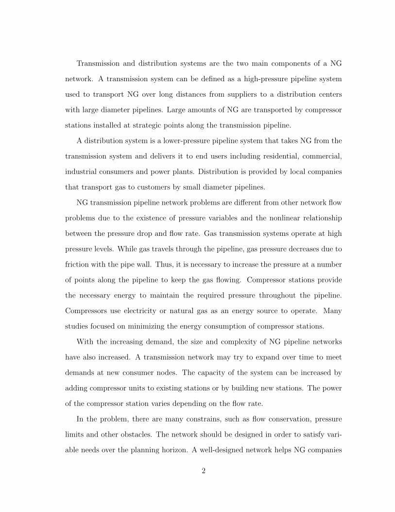
Transmission and distribution systems are the two main components of a NG
network. A transmission system can be defined as a high-pressure pipeline system
used to transport NG over long distances from suppliers to a distribution centers
with large diameter pipelines. Large amounts of NG are transported by compressor
stations installed at strategic points along the transmission pipeline.
A distribution system is a lower-pressure pipeline system that takes NG from the
transmission system and delivers it to end users including residential, commercial,
industrial consumers and power plants. Distribution is provided by local companies
that transport gas to customers by small diameter pipelines.
NG transmission pipeline network problems are different from other network flow
problems due to the existence of pressure variables and the nonlinear relationship
between the pressure drop and flow rate. Gas transmission systems operate at high
pressure levels. While gas travels through the pipeline, gas pressure decreases due to
friction with the pipe wall. Thus, it is necessary to increase the pressure at a number
of points along the pipeline to keep the gas flowing. Compressor stations provide
the necessary energy to maintain the required pressure throughout the pipeline.
Compressors use electricity or natural gas as an energy source to operate. Many
studies focused on minimizing the energy consumption of compressor stations.
With the increasing demand, the size and complexity of NG pipeline networks
have also increased. A transmission network may try to expand over time to meet
demands at new consumer nodes. The capacity of the system can be increased by
adding compressor units to existing stations or by building new stations. The power
of the compressor station varies depending on the flow rate.
In the problem, there are many constrains, such as flow conservation, pressure
limits and other obstacles. The network should be designed in order to satisfy vari-
able needs over the planning horizon. A well-designed network helps NG companies
2
minimize the costs while increasing the customer service level. Thus, a good opti-
mization tool is important to make strategic and operational decisions.
The main thrust of this research is the development of a decision support tool to
aid system operators in optimizing NG pipeline operations and the investment costs
in order to satisfy customer demand with minimal costs.
1.1 Research Objectives and Scope
In NG pipeline networks, design and expansion decisions must be made with care-
ful consideration of the long term benefits. The investment and operating costs, such
as installing and operating pipelines and compressor stations, are very high. Com-
pressor station and pipeline installations are part of long-term strategic decisions.
Once they are built, they will operate for years. It may cost more than expected to
maintain them if these decisions are not made carefully. The aim of this study is
to minimize the total investment and operating costs while satisfying the specified
requirements corresponding to demands and pressure limits in the system.
The solution to the problem will help to make decisions regarding a new trans-
mission network design, as well as expansion of an existing network, with minimized
total cost. In this study, an optimization model is provided to address the following
issues:
1. Pressure requirements
2. The best location and capacity of compressor stations that minimizes the cost
3. The best location of pipelines that minimizes the cost
4. The scheduling of installing pipelines and compressor stations in the network
5. The best amount of NG procurement from available suppliers
3
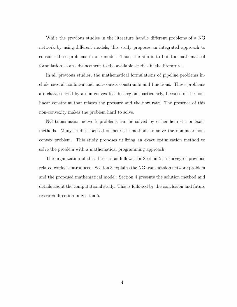
While the previous studies in the literature handle different problems of a NG
network by using different models, this study proposes an integrated approach to
consider these problems in one model. Thus, the aim is to build a mathematical
formulation as an advancement to the available studies in the literature.
In all previous studies, the mathematical formulations of pipeline problems in-
clude several nonlinear and non-convex constraints and functions. These problems
are characterized by a non-convex feasible region, particularly, because of the non-
linear constraint that relates the pressure and the flow rate. The presence of this
non-convexity makes the problem hard to solve.
NG transmission network problems can be solved by either heuristic or exact
methods. Many studies focused on heuristic methods to solve the nonlinear non-
convex problem. This study proposes utilizing an exact optimization method to
solve the problem with a mathematical programming approach.
The organization of this thesis is as follows: In Section 2, a survey of previous
related works is introduced. Section 3 explains the NG transmission network problem
and the proposed mathematical model. Section 4 presents the solution method and
details about the computational study. This is followed by the conclusion and future
research direction in Section 5.
4

2. LITERATURE REVIEW
In the literature, there are three main network problems which are used to handle
different challenges in NG transmission networks.
In NG network design problems, the objective function may be minimization
of the investment cost or maximization of the net present value. The output of the
model helps to locate the optimal type and the number of compressor stations, and to
select the optimal pipe dimensions. Several design variables need to be determined.
They include the location and type of compressor stations; possible locations, lengths
and diameter of pipelines to be installed; and the allowable operating pressure levels
of the system.
NG network flow problems aim to minimize costs and meet demand. Decision
variables of the problem are defined to determine gas flow through the pipeline
network. The operation cost of NG transmission systems is highly dependent on the
compressor station operations because the amount of NG in the system is set by
compressor stations. In these problems, selecting the optimal compressor location
and capacity is a critical decision.
In network expansion problems, the objective is generally scheduling the invest-
ments. To obtain the optimum capacity expansion, investment decisions including
time, size and location of pipeline and compressor station installations should be
made [14].
This research is based on a comprehensive study that combines three network
problems in one model. The main focus is to design a new NG transmission pipeline
network or to expand the existing network in order to minimize the investment and
operating costs of transporting gas through pipelines in multiple periods.
5

Many studies have been done in pipeline network optimization including the
pipeline network design, the minimization of fuel consumption of compressor stations,
economically locating compressor stations in the network.
Rios-Mercado et al. [24] proposed a reduction technique to minimize the fuel
consumption of compressor stations in steady-state transmission networks. This
method minimizes the problem dimension at preprocessing without disrupting the
problem structure. De Wolf and Smeers [11] modeled the NG pipeline network with
nonlinear and linear constraints for a cost minimization problem. They developed a
successive linear programming method. The solution procedure is based on piecewise
linear approximations of the nonlinear constraint that defines the relationship of the
pressure and flow rate. Three test problems with 24, 34 and 60 arcs are solved
by an extension of the simplex algorithm. Wu et al. [33] also studied the fuel cost
minimization problem. They derived two model relaxations. One relaxation is to
develop linear supersets of the non-convex nonlinear compressor domain. The other
is to derive piecewise linear functions of the fuel cost objective function. They tested
the method by three examples. The first example is a six-node, three-pipe, two-
compressor network. The second example is a simple tree network with 10 nodes,
6 pipes, and 3 compressor stations and in the third example there are 48 nodes, 43
pipes, and 8 stations.
Most of the methods developed for this minimization of the fuel consumption
problem are based on dynamic programming and gradient search methods. The dy-
namic programming method was first proposed for a steady state gas transmission
system by Wong and Larson [32]. In the study, DP was used to optimize the single
source tree-structured network. The objective is to minimize the total compressor
energy required to satisfy the specified flow rate, pressure and compressor operation
constraints. Dynamic programming guarantees the global optimum. Also, nonlin-
6
earity can be easily solved by dynamic programming. However, the implementation
of dynamic programming is limited to simple network structures, and computational
time increases with the problem size. Two problems were used to represent the per-
formance of the proposed method, one with a single pipeline that has 10 compressors
and the other with three single pipelines and a total of 23 compressors.
The study of Borraz-Sanchez and Rios-Mercado [6] aims to find the optimal so-
lution for the compressor station operations in the cyclic NG pipeline network while
minimizing the fuel consumption of the stations. The network is represented by
pipeline and compressor station arcs and corresponding nodes at the intersection
points of the arcs. In the model, there are two continuous decision variables; mass
flow rates in each arc and gas pressure at each node. Constraints are non-convex and
the objective function is nonlinear. That is, the problem is modeled as a nonlinear
program. The proposed solution method is the combination of the non-sequential
dynamic programming and the tabu search algorithm. They used various test in-
stances to evaluate the proposed method. The larger problem size has 19 nodes and
7 compressor station arcs.
In other studies, heuristic approaches were proposed in order to minimize com-
pressor station costs. The ant colony optimization algorithm is used for the first
time for studying gas flow operations in the study of Chebouba et al. [8]. The main
focus of this paper is on using ant colony optimization as a decision tool to obtain
fast and accurate results. The objective function of the problem is nonlinear and
non-convex. Test instance is composed of one source, one demand and 6 pipelines
connected in series by 5 compressor stations. The main interest of the study of Rios-
Mercado et al. [23] is the gas transmission problems with a cyclic tree structure. In
this paper a heuristic solution algorithm is proposed. The methodology is composed
of two stages. At the first stage, dynamic programming is used to find optimal val-
7
ues for pressure variables while the flow variables are fixed. At the second stage,
using the optimal value of a pressure variable found at the first stage, a set of flow
values, which improve the objective value, are found by a heuristic approach. The
proposed method was tested on a tree structured system with 64 nodes, 56 pipes,
and 16 compressor stations.
Chung et al. [9] proposed a multi-objective mathematical programming method.
Investment costs, reliability and environmental impact compose the three different
objectives of the model. They solved the problem by genetic algorithm and adopted
a fuzzy decision method to select the best network planning scenario. The model was
applied to a network with 13 compressor stations, and 19 pipelines. A hierarchical
algorithm is proposed by Hamedi et al. [13] to solve a distribution network problem by
using a single-objective, multi-period mixed integer nonlinear programming (MINLP)
model. They converted the model into a MIP by adding a set of constraints. The
objective is to minimize direct and indirect costs. The model was tested for se seven
samples. The smallest test instance include 190 nodes and the largest one has 319
nodes. A MIP model is proposed by Uraikul et al. [28] to optimize the operations of
selecting and controlling the compressors. The objective of the study is to minimize
the operating costs of the network and meet customer demands in the system. The
three factors that affect the costs are the capacities of compressors, the energy used
to turn on the compressors, and the energy used to turn them off. The model was
tested on a network that has two compressor stations, two customer locations and
six periods.
Kabirian and Hemmati [15] developed an integrated nonlinear optimization model
for formulating a strategic plan to find the best long-run development plans for an
existing network. A heuristic random search optimization method is proposed to
solve the problem. The objective is to minimize the net present value of operating
8
and investment costs. They used a network with 2 compressor stations, 4 demand,
3 supply and 1 transshipment nodes, and 10 pipelines to assess the performance of
the model.Pratt and Wilson [22] propose a mixed integer linear programming (MIP)
method to solve the nonlinear optimization problem iteratively. They linearized the
pressure drop-flow equation and used the branch-and-bound (BB) algorithm to solve
the problem. Osiadacz and Bell [21] suggest a simplified algorithm for the transient-
state gas transmission network to find the maximum feasible outlet pressure level of
a station. They studied a large-scale network with several compressor stations and
they solved the problem by local optimization.
Woldeyohannes and Majid [31] developed a simulation model by incorporating
compressor station parameters including speed, suction and discharge pressure. The
model is used to simulate the transmission pipeline network system under various
conditions to determine pressure and flow parameters. The proposed simulation
model in this study could be used to assist in operational and design decisions.
The review of papers in the scope of optimization in NG transmission network
based on the decisions made are classified in Table 2.1. Table 2.2 is a summary of
the NG network optimization problems.
9
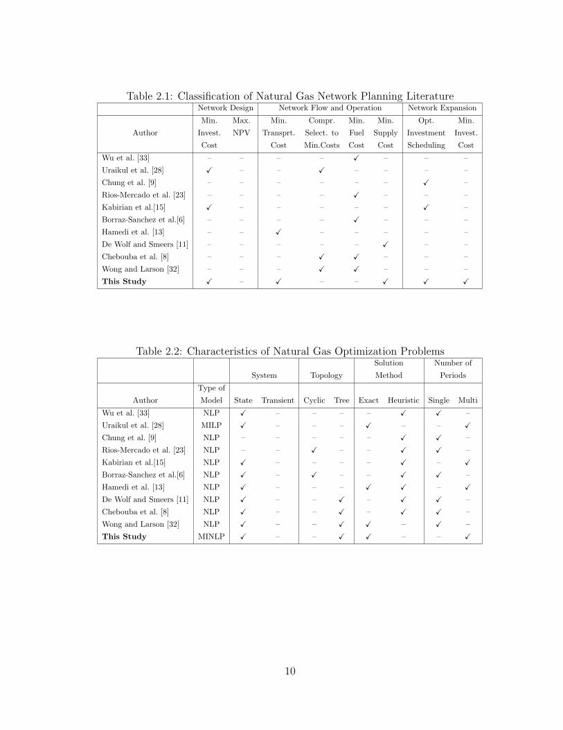
Table 2.1: Classification of Natural Gas Network Planning LiteratureNetwork Design Network Flow and Operation Network Expansion
Min. Max. Min. Compr. Min. Min. Opt. Min.
Author Invest. NPV Transprt. Select. to Fuel Supply Investment Invest.
Cost Cost Min.Costs Cost Cost Scheduling Cost
Wu et al. [33] – – – – X – – –
Uraikul et al. [28] X – – X – – – –
Chung et al. [9] – – – – – – X –
Rios-Mercado et al. [23] – – – – X – – –
Kabirian et al.[15] X – – – – – X –
Borraz-Sanchez et al.[6] – – – – X – – –
Hamedi et al. [13] – – X – – – – –
De Wolf and Smeers [11] – – – – – X – –
Chebouba et al. [8] – – – X X – – –
Wong and Larson [32] – – – X X – – –
This Study X – X – – X X X
Table 2.2: Characteristics of Natural Gas Optimization ProblemsSolution Number of
System Topology Method Periods
Type of
Author Model State Transient Cyclic Tree Exact Heuristic Single Multi
Wu et al. [33] NLP X – – – – X X –
Uraikul et al. [28] MILP X – – – X – – X
Chung et al. [9] NLP – – – – – X X –
Rios-Mercado et al. [23] NLP – – X – – X X –
Kabirian et al.[15] NLP X – – – – X – X
Borraz-Sanchez et al.[6] NLP X – X – – X X –
Hamedi et al. [13] NLP X – – – X X – X
De Wolf and Smeers [11] NLP X – – X – X X –
Chebouba et al. [8] NLP X – – X – X X –
Wong and Larson [32] NLP X – – X X – X –
This Study MINLP X – – X X – – X
10

3. PROBLEM DEFINITION AND MATHEMATICAL FORMULATION
A typical NG pipeline network problem consists of demand and supply nodes,
pipelines, and compressor stations. In such complex and large networks, proper
planning is important because even a small reduction in investment and operation
expenses provides considerable amounts of saving. NG networks continue to grow
with the increasing demand and this growth makes the network more complex. Thus,
developing effective solution methods becomes more important.
An optimization approach is proposed to solve the problem of how to optimally
design the network and operate the gas flow in the pipeline system with deterministic
parameters. In this study, it is assumed that the transmission system, consisting of
multiple suppliers and multiple consumers, is operated only by the NG Company.
3.1 Characteristics of the System
There are two different states in the gas network depending on the gas flow-time
relationship. If a system is in a steady state, then gas flow through the system is
independent of time. These systems can be modeled by algebraic nonlinear equa-
tions. In a transient state system, gas flow changes in time, thus, partial differential
equations are required to describe this relation. In this research, a steady-state gas
transmission network system will be studied.
Another characteristic of transmission systems is the topology of the network.
There are two main structure types of gas networks. A cyclic topology is a network
with at least one cycle. A tree structured (non-cyclic) topology is a network that does
not contain any cycles. These networks may contain a number of different trees. The
main focus of the study will be on the transmission of gas through a tree-structured
pipeline network system.
11

A NG transmission network studied in this research consists of demand, sup-
ply, transshipment, and compressor station inlet and outlet nodes. In the network,
pipelines and compressor stations are represented by directed arcs. Demand nodes
are the locations of NG consumer cities. Supply nodes are the sources of gas. Trans-
shipment nodes are the connection points of two or more arcs. In transshipment
nodes, incoming flow is equal to outgoing flow. Compressor station inlet nodes are
the points where gas enters a station. Compressor station outlet nodes are the end
points of compressor station arcs where compressed gas exits a station. The impacts
of other elements including valves and regulators are negligible for this study.
Figure 3.1 show the graphical notation of the network.
Supply Node
Demand Node
Transshipment Node
Active Pipe Arcs
Inactive Pipe Arcs
Closed Compressor Station
Bypassed Compressor Station
Active Compressor Station
Figure 3.1: Graphical Notation for the Networks
12

Figure 3.2: A Natural Gas Transmission Pipeline Network
A typical network of the problem with 11 nodes, 9 pipe arcs, and 1 compressor
arc is shown in Figure 3.2. Node S is a supply node, where gas is purchased from.
Node D1, D2, D3, D4, D5, and D6 are demand nodes, where gas is consumed. Node
A is a transmission node. Nodes CS-Ent and CS-Ext are compressor station inlet
and outlet nodes, respectively.
In the proposed model, there are several decision variables related to the compo-
nents of the system. The positive continuous variables are pressures at nodes, gas
flow rates in pipelines and the supply amount. The sets of binary variables are used
to define the flow directions, compressor station locations and types, and pipeline
locations.
The objective is to minimize the total investment and operating cost of the net-
work. Investment costs are the installation costs of pipelines and compressor stations.
Operating costs consist of transporting cost, operation cost of compressor stations
and pipelines, such as maintenance, energy, etc., and purchase cost of supply. The
costs are varied for each period so the total cost is the sum of periodic costs.
13

The mathematical model of the problem is a MINLP, where the objective func-
tion is linear and the set of constraints including linear and nonlinear inequalities
with binary and continuous variables. The model includes various linear constraints
for mass flow conservation for supply, demand and transshipment nodes. Pressure-
flow rate relation will be defined by nonlinear inequalities. Moreover, there will be
constraints related to whether compressor station existence and to its capacity.
The problem is described as a multi-period network problem model in order to
allow making changes in the network over the planning horizon. These changes can
be exogenous, i.e. the existence of new demand nodes, in response to increasing
demand. As a result of these, new endogenous changes may be needed such as
adding new pipelines, and compressor stations. It is assumed that these changes are
long-lasting, which means once a new pipeline/compressor station is installed, or a
new demand node is added to the network, then it is available during all planning
horizons in the network.
3.2 System Components
3.2.1 Pipelines
The relationship between the flow rate and the pressure, and the definition of
pressure values as state variables at nodes, are the major characteristics of the trans-
mission network in steady-state. Flow rate is a function of the pressure difference
across the pipe, the diameter and length of the pipe, and properties of gas. Using
the same function, the pressure values can be determined by flow rate and pipeline
resistance.
The properties of pipelines and gas are important to determine the pipeline re-
sistance so the pipeline resistance determines the pressure drop. While gas flows,
pressure decreases due to pipeline resistance and flow losses. At every demand node,
14

the amount of flow in the pipeline decreases as well as the pressure. The pressure
difference between the end nodes of a pipeline depends on the resistance.
Several variations of the general flow equation have been proposed to calculate
the gas flow rate in a pipeline, such as the Weymouth equation, the Panhandle A and
Panhandle B equations [20]. These equations differ from each other by the system
size range they can be applied to and the treatment of pipe friction. The General
Flow Equation for the steady-state flow in a gas pipeline is the basic equation for
relating the pressure drop to flow rate. In the system, gas flows at a constant tem-
perature (isothermal flow) through a horizontal pipe segment. The pipe segments
are assumed to be long enough so that kinetic energy changes can be negligible [16].
Figure 3.3 shows a steady flow in the gas pipeline.
Figure 3.3: Steady Flow in Gas Pipeline
In The International System of Units (SI) units, the General Flow equation is
stated as follows:
Qij = 1.1494 10−3(TbPb
)2 [ P 2i − P 2
j
GTfLijZf
]0.5D2.5
ij (3.1)
where friction factor (f), base pressure (Pb) and temperature (Tb), gas gravity (G),
average gas flowing temperature (Tf ), gas compressibility factor (Z) are assumed to
15

be constants. This equation can be applied where fully turbulent gas flow under high
pressure is in question [20].
Equation relates the flow rate in a pipe with a length L (km) and a diameter D
(mm), based on an upstream pressure Pi (bar) and a downstream pressure Pj (bar).
The flow rate Q (m3/day) depends on gas properties such as the gravity G (0.66 for
NG) and the compressibility factor Z (0.805 for NG). The pressure drop, from the
upstream point i to downstream point j, occurs due to friction between the gas and
pipe walls with a typical friction factor f (generally 0.01). The pressure difference of
the two nodes, the upstream end and the downstream end, determines the direction
of the gas flow. When there is no flow rate between nodes i and j, Pi is equal to Pj.
Since the volume of gas changes according to the ambient temperature and pressure,
base temperature Tb (◦K) and pressure Pb (bar) are necessary to provide standard
conditions for gas measurement. In this study, base temperature Tb is 288◦K and
base pressure is Pb is 1 bar while the average gas flowing temperature Tf is 283◦K.
It is assumed that the unit of flow rate Q is million cubic meters (mmscm), so all
calculations in this study are made accordingly. The studied transmission network
is composed of horizontal pipelines. In transmission networks, pipe sizes generally
vary between 12 and 48 inches in diameter, 5 and 100 km in length. In this study,
the diameter of pipelines are assumed to be fixed to 30 inches, but the lengths are
variable. In The pipe flow equation that relates the pressure drop to the flow rate of
high pressure flows in a steady state is represented as
P 2it − P 2
jt = δij Q2ijt ∀ (i, j) ∈ AP (3.2)
where the value of δij (pipeline resistance) depends on the properties of gas and also
the dimensions of the pipe (i, j).
16

In this study, the general flow equation is used to calculate the pressure drop.
Thus, the pipeline resistance can be expressed as
δij = 0.7569 106 GTfLijZf
D5ij
(Pb
Tb
)2
∀ (i, j) ∈ AP (3.3)
As mentioned earlier, pressure drop and flow rate depend on pipeline properties.
Thus, it is often necessary to decide pipe sizes before calculating pressure drop and
flow rate. The pressure levels at nodes can be calculated, by knowing the flow rate
and available pipe sizes in advance. Then, the compressor stations can be located at
necessary points.
As the pipe length increases for a given flow rate, the pipeline resistance increases
as well as the pressure drop. For pipes of the same diameter, the pressure difference
is greater between two ends of a long one than a shorter one. On the other hand, a
pipe with a large diameter has less resistance than a pipe with a smaller diameter.
Thus, the pressure drop is smaller across a pipe with a large diameter [20].
3.2.2 Compressor Stations
Compressor stations are one of the most important assets in transmission pipeline
network systems worldwide. They are installed to provide the pressure needed to
transport gas through pipelines. They can be defined simply as a device to com-
press gas molecules in order to provide enough energy to keep it moving along the
transmission line. Due to the limitations of pipeline pressures, multiple compressor
stations may be needed to transport a given volume through a long-distance pipeline.
The pressures at which these compressor stations operate are determined by the pipe
pressure levels and the power available [20]. In this study, the set of nodes repre-
senting compressor stations consists of inlet (CS-Ent) and outlet (CS-Ext) nodes.
17
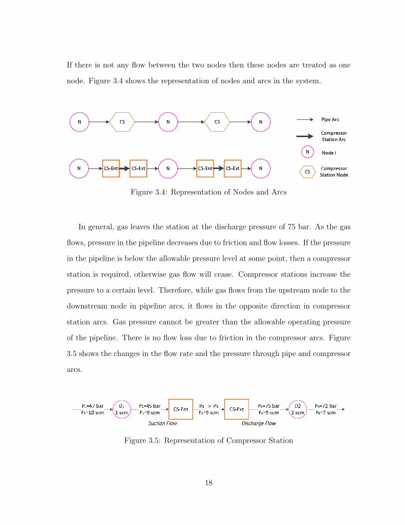
If there is not any flow between the two nodes then these nodes are treated as one
node. Figure 3.4 shows the representation of nodes and arcs in the system.
Figure 3.4: Representation of Nodes and Arcs
In general, gas leaves the station at the discharge pressure of 75 bar. As the gas
flows, pressure in the pipeline decreases due to friction and flow losses. If the pressure
in the pipeline is below the allowable pressure level at some point, then a compressor
station is required, otherwise gas flow will cease. Compressor stations increase the
pressure to a certain level. Therefore, while gas flows from the upstream node to the
downstream node in pipeline arcs, it flows in the opposite direction in compressor
station arcs. Gas pressure cannot be greater than the allowable operating pressure
of the pipeline. There is no flow loss due to friction in the compressor arcs. Figure
3.5 shows the changes in the flow rate and the pressure through pipe and compressor
arcs.
Figure 3.5: Representation of Compressor Station
18
A compressor station may be active, bypassed or closed. These states will be
decided according to the solution of the problem. If the outlet pressure value is
greater than the inlet pressure value at the compressor nodes, then the station is
active. When the outlet and inlet pressure values are equal, the station is bypassed.
If there is no flow through the compressor arc, then the compressor station is closed.
While designing a pipeline system, the possible locations and sizes of the compres-
sor stations must be determined. The size of a compressor station, or, more precisely
the number of units that must be installed, depends on the mass flow rate. In this
study, it is assumed that compressor units installed in a station are identical, and the
maximum flow rate between two compressor station nodes is 20 mmscm/day. The
number of stations in the system depends on the length of the transmission pipeline.
More stations are required if the length of the line increases. Environmental and
geotechnical factors are important in selecting the station location.
3.2.3 Cost Structure
In pipeline network problems, generally, the cost function consists of investment
and operating costs. The major components of the gas transmission system that ac-
count for the investment costs are the pipeline and compressor stations. These costs
constitute the important part of the total pipeline project cost. Operating costs, such
as maintenance, energy, transmission, utility, as well as general and administrative,
are the recurring periodic costs.
The total cost for gas transmission pipeline network can be calculated as follows;
Total Cost = [investment cost + operating cost ]pipeline
+ [investment cost + operating cost ]compressor station
+ natural gas purchase cost + transportation cost
(3.4)
19
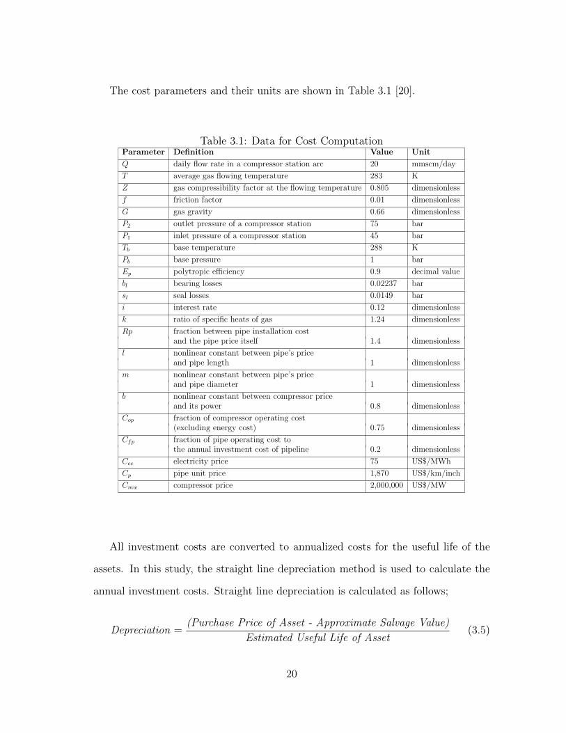
The cost parameters and their units are shown in Table 3.1 [20].
Table 3.1: Data for Cost ComputationParameter Definition Value Unit
Q daily flow rate in a compressor station arc 20 mmscm/day
T average gas flowing temperature 283 K
Z gas compressibility factor at the flowing temperature 0.805 dimensionless
f friction factor 0.01 dimensionless
G gas gravity 0.66 dimensionless
P2 outlet pressure of a compressor station 75 bar
P1 inlet pressure of a compressor station 45 bar
Tb base temperature 288 K
Pb base pressure 1 bar
Ep polytropic efficiency 0.9 decimal value
bl bearing losses 0.02237 bar
sl seal losses 0.0149 bar
i interest rate 0.12 dimensionless
k ratio of specific heats of gas 1.24 dimensionless
Rp fraction between pipe installation costand the pipe price itself 1.4 dimensionless
l nonlinear constant between pipe’s priceand pipe length 1 dimensionless
m nonlinear constant between pipe’s priceand pipe diameter 1 dimensionless
b nonlinear constant between compressor priceand its power 0.8 dimensionless
Cop fraction of compressor operating cost(excluding energy cost) 0.75 dimensionless
Cfp fraction of pipe operating cost tothe annual investment cost of pipeline 0.2 dimensionless
Cec electricity price 75 US$/MWh
Cp pipe unit price 1,870 US$/km/inch
Cmw compressor price 2,000,000 US$/MW
All investment costs are converted to annualized costs for the useful life of the
assets. In this study, the straight line depreciation method is used to calculate the
annual investment costs. Straight line depreciation is calculated as follows;
Depreciation =(Purchase Price of Asset - Approximate Salvage Value)
Estimated Useful Life of Asset(3.5)
20

It is assumed that the entire life of the system is 45 years and the salvage values
of the assets are zero at the end of the life of the assets. The net present values of
the annual investments in the first 12 years are computed based on a 12% interest
rate. Net present value is expressed as
NPV = C0 −T∑t=1
Ct
(1 + i)t(3.6)
3.2.3.1 INVESTMENT COST FOR PIPELINE
The investment cost of the pipeline including the material, labor, installation,
and right of way costs, depends on pipe length and diameter [1] . It can be expressed
as
αpt = (1 +Rp)Cp length
l diam (3.7)
The value of Cp, l,m can be found easily by regression if the price of pipe is
known. In this study, they are assumed to be 1.
3.2.3.2 INVESTMENT COST FOR COMPRESSOR STATIONS
To build the objective function, it is assumed that electricity is used to operate
the compressor stations. Tax, insurance, and other costs are not included in the
cost function. The fixed compressor station cost changes depending on the installed
power (MW). The following is the expression for compressor power [1] .
gmw = 3.0325QPbTZ
[(P2
P1)( k−1kEp
) − 1]k
Tb(k − 1)+ bl + sl (3.8)
21

where Q is the daily flow rate in a compressor station arc. The investment cost of
compressor stations is computed as follows
αct = Cmw(gmw)b (3.9)
where Cmw is a overall cost of material, equipment, labor, right of way per 1 MW.
Cmw and b values can be found by regression as well.
By using the given parameters, the power of each compressor station unit is 10
MW.
3.2.3.3 PIPELINE OPERATING COST
The pipeline operating cost is the cost of maintaining pipes. It is assumed the
operating cost is proportional to the annual investment cost [1]. For each pipeline
segment the operating cost is computed as follows;
βpt = Cfp α
pt (3.10)
3.2.3.4 COMPRESSOR STATION OPERATING COST
The operating cost of a compressor station is electricity and maintenance cost.
The operating cost can be formulated as a proportional to the electricity cost [1] .
Thus, it is expressed as follows;
βct = (1 + Cop)Cec (3.11)
To calculate the electricity cost, the unit of compressor power is converted into
megawatt-hour, then
22
gMWh = 19.809QPbTZ
[(P2
P1)( k−1kEp
) − 1]k
Tb(k − 1)+ 6.532(bl + sl) (3.12)
and the electricity cost is
Cec = gMWhCe (3.13)
At the beginning of the planning horizon the electricity price is 75$/MWh. It is
assumed that the electricity price increases 5% each year.
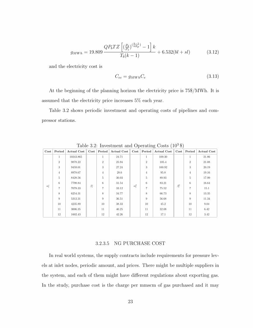
Table 3.2 shows periodic investment and operating costs of pipelines and com-
pressor stations.
Table 3.2: Investment and Operating Costs (103 $)Cost Period Actual Cost Cost Period Actual Cost Cost Period Actual Cost Cost Period Actual Cost
αct
1 10243.865
βct
1 24.71
αpt
1 109.30
βpt
1 21.86
2 9878.22 2 25.94 2 105.4 2 21.08
3 9459.01 3 27.24 3 100.92 3 20.19
4 8978.67 4 28.6 4 95.8 4 19.16
5 8428.56 5 30.03 5 89.93 5 17.99
6 7798.84 6 31.54 6 83.21 6 16.64
7 7078.33 7 33.12 7 75.52 7 15.1
8 6254.31 8 34.77 8 66.73 8 13.35
9 5312.31 9 36.51 9 56.68 9 11.34
10 4235.89 10 38.33 10 45.2 10 9.04
11 3006.35 11 40.25 11 32.08 11 6.42
12 1602.43 12 42.26 12 17.1 12 3.42
3.2.3.5 NG PURCHASE COST
In real world systems, the supply contracts include requirements for pressure lev-
els at inlet nodes, periodic amount, and prices. There might be multiple suppliers in
the system, and each of them might have different regulations about exporting gas.
In the study, purchase cost is the charge per mmscm of gas purchased and it may
23

vary for each supplier [1]. Gas purchase cost is assumed to increase 2% each year.
Table 3.3 shows purchase cost of each supplier in each period.
Table 3.3: Purchase Costs (103 $)Period Supplier 1 Supplier 2 Supplier 3 Supplier 4
1 250.00 300.00 350.00 275
2 255.00 306.00 357.00 280.50
3 260.10 312.12 364.14 286.11
4 265.30 318.36 371.42 291.83
5 270.61 324.73 378.85 297.67
6 276.02 331.22 386.43 303.62
7 281.54 337.85 394.16 309.70
8 287.17 344.61 402.04 315.89
9 292.92 351.50 410.08 322.20
10 298.77 358.53 418.28 328.65
11 304.75 365.70 426.65 335.22
12 310.84 373.01 435.18 341.93
3.2.3.6 TRANSPORTATION COST
Since transportation is a major component of the total cost of the system, many
studies on transmission pipeline properties are promoted in order to find an optimum
system design for economical transmission. For every unit of gas transported, the
pipeline owner pays the transportation cost to maintain the transportation. The
transportation cost can be defined as the cost of service to transport a unit of gas
through a segment of pipeline. The transportation cost is charged per mmscm of
gas. It is expressed as
βst =
(∑
i,j lengthij(βpt + αp
t )) + βct + αc
t
Fijt
(3.14)
24
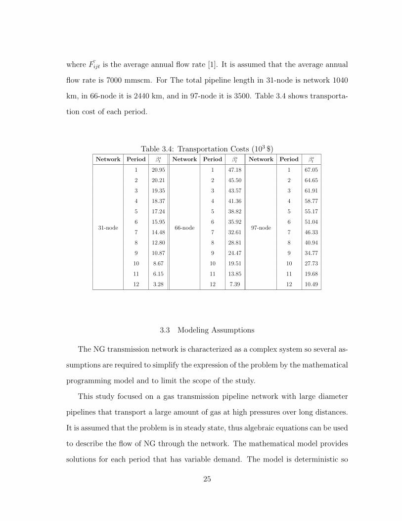
where Fijt is the average annual flow rate [1]. It is assumed that the average annual
flow rate is 7000 mmscm. For The total pipeline length in 31-node is network 1040
km, in 66-node it is 2440 km, and in 97-node it is 3500. Table 3.4 shows transporta-
tion cost of each period.
Table 3.4: Transportation Costs (103 $)Network Period βs
t Network Period βst Network Period βs
t
31-node
1 20.95
66-node
1 47.18
97-node
1 67.05
2 20.21 2 45.50 2 64.65
3 19.35 3 43.57 3 61.91
4 18.37 4 41.36 4 58.77
5 17.24 5 38.82 5 55.17
6 15.95 6 35.92 6 51.04
7 14.48 7 32.61 7 46.33
8 12.80 8 28.81 8 40.94
9 10.87 9 24.47 9 34.77
10 8.67 10 19.51 10 27.73
11 6.15 11 13.85 11 19.68
12 3.28 12 7.39 12 10.49
3.3 Modeling Assumptions
The NG transmission network is characterized as a complex system so several as-
sumptions are required to simplify the expression of the problem by the mathematical
programming model and to limit the scope of the study.
This study focused on a gas transmission pipeline network with large diameter
pipelines that transport a large amount of gas at high pressures over long distances.
It is assumed that the problem is in steady state, thus algebraic equations can be used
to describe the flow of NG through the network. The mathematical model provides
solutions for each period that has variable demand. The model is deterministic so
25

each parameter is assumed to be known in advance. The model is built on a cyclic
network, but the output of the model is a tree network. Therefore, there are no loops
in the output.
Since a gas transmission network problem is also a network flow problem, mass
flow conservation must be satisfied in the system. The key characteristic of the prob-
lem is the presence of pressure variables. The allowed maximum pressure depends
on a Gas Company’s needs. In the network, pressure requirements will be met and
NG will be forced to flow in one direction per period.
3.4 Network Structure
The transmission pipeline network is modeled in a directed graph G = (N,A).
N is a finite set of nodes; i ∈ {1, 2, . . . , |N |} and it consists of supply (Ns), demand
(Nd), transshipment (Nt), compressor station inlet and outlet nodes (Nc). The set
of nodes can be defined as N = Ns ∪Nd ∪Nt ∪Nc. A is a set of arcs, which are the
ordered pairs (i, j) of distinct nodes in N . A is a union set of pipe and compressor
station arcs in the network, i.e., A = Ap ∪ Ac, with Ap ∩ Ac = ∅. If (i, j) ∈ Ac
then i, j ∈ Nc are the nodes representing the inlet and outlet nodes of a compressor
station. A similar interpretation can be made for pipeline arcs (i, j) ∈ Ap where
i, j ∈ N .
Pipeline arcs function with different gas flows between two nodes to satisfy chang-
ing customer demands over multi-period. The network must contain at least one pipe
arc connected to a demand node. Since the network is described as a directed graph,
back-flow in the pipes is not allowed. Pressure decreases along the pipe arcs, while
it increases along the compressor station arcs. In the following, the problem is for-
mulated as a MINLP model.
26

3.5 The Mathematical Model
The mathematical formulation of the gas transmission network problem is given
as follows;
NOTATIONS:
Sets:
T set of periods
U set of the number of compressor stations units
Ns set of supply nodes
Nd set of demand nodes
Nt set of transshipment nodes
Nc compressor station nodes
N the union of sets Ns, Nd, Nt, andNc
Ac set of compressor station arcs
Ap set of pipeline arcs
E the union of sets Ac and Ap
Parameters:
θi demand of ith node in period t ∈ Tδij pipeline resistance between nodes (i, j) ∈ Ap
αct investment cost of installing one unit of a compressor station in period t ∈ Tαpt investment cost of installing a pipeline in period t ∈ Tβct operating cost of one unit of a compressor station in period t ∈ Tβpt operating cost of one km of a pipeline arc in period t ∈ Tβst transportation cost t ∈ Tβfit NG purchase cost of supplier i ∈ Ns t ∈ Tσ capacity of one unit of a compressor station
φij length of available pipelines (i, j) ∈ Ap
27

Decision Variables:
Pit pressure at node i in period t ∈ TQijt mass flow rate between nodes i and j in period t ∈ TBijt 1 if gas flows from i to j in period t ∈ T , 0 otherwise
CSijut 1 if a compressor station is installed at nodes (i, j) ∈ Nc
with u units in period t ∈ T , 0 otherwise
Vijt 1 if a new pipeline is installed between nodes i and j in period t ∈ T ,
0 otherwise
Git 1 if the pressure is below 45 bar at node i ∈ Nc in period t ∈ T ,
0 otherwise
MODEL:
Min∑
(i,j)∈Ap
∑t∈T
Qijtβst +
∑i∈Ns
∑j∈N
∑t∈T
Qijtβfit +
∑(i,j)∈Ac
∑u∈U
∑t∈T
uCSijutβct
+∑
(i,j)∈Ap
i<j
∑t∈T
φijVijtβpt +
∑(i,j)∈Ap
i<j
|T |−1∑t=0
φij(Vijt+1 − Vijt)αpt+1
+∑
(i,j)∈Ac
∑u∈U
|T |−1∑t=0
u(CSijut+1 − CSijut)αct+1
(3.15)
subject to
Pit = 75 ∀ i ∈ Ns, t ∈ T (3.16)
Bijt ≤M Qijt ∀ (i, j) ∈ E, t ∈ T (3.17)
Qijt ≤M Bijt ∀ (i, j) ∈ E, t ∈ T (3.18)
Bijt +Bjit ≤ 1 ∀ (i, j) ∈ E, i < j, t ∈ T (3.19)
Pjt − Pit ≤M (1−Bijt) ∀ (i, j) ∈ Ap, t ∈ T (3.20)
28

∑(i,j)∈E
Qjit −∑
(i,j)∈E
Qijt = qit ∀ i ∈ Nd, t ∈ T (3.21)
∑(i,j)∈E
Qjit −∑
(i,j)∈E
Qijt = 0 ∀ i ∈ Nt ∪Nc, t ∈ T (3.22)
∑(i,j)∈E
Qijt ≥ 0 ∀ i ∈ Ns, t ∈ T (3.23)
(P 2it − P 2
jt)− δij Q2ijt ≥M (Bijt − 1) ∀ (i, j) ∈ Ap, t ∈ T (3.24)
(P 2it − P 2
jt)− δij Q2ijt ≤M (1−Bijt) ∀ (i, j) ∈ Ap, t ∈ T (3.25)
Bijt +Bjit ≤ Vijt ∀ (i, j) ∈ Ap, t ∈ T, i ≤ j (3.26)
Vijt ≤ Vijy ∀ (i, j) ∈ Ap, i ≤ j, t ∈ T,
y ∈ T, t ≤ y (3.27)
45− Pit ≤M Git ∀ i ∈ N, t ∈ T (3.28)
Bijt +Git − 1 ≤∑u∈U
CSijut ∀ (i, j) ∈ Ac, t ∈ T (3.29)
∑u∈U
CSijut ≤ 1 ∀ (i, j) ∈ Ac, t ∈ T (3.30)
Bijt −∑u∈U
CSijut ≥ 0 ∀ (i, j) ∈ Ac, t ∈ T (3.31)
∑u∈U
CSijut +∑u∈U
CSjiut ≤ 1 ∀ (i, j) ∈ Ac, i < j, t ∈ T (3.32)
CSijut ≤ CSijuy ∀ (i, j) ∈ Ac, i < j, t ∈ T,
y ∈ T, t ≤ y, u ∈ U (3.33)
Pjt − (75∑u∈U
CSijut)− Pjt(1−∑u∈U
CSijut) ≥M (Bijt − 1) ∀ (i, j) ∈ Ac, t ∈ T
(3.34)
29

Pjt − (75∑u∈U
CSijut)− Pjt(1−∑u∈U
CSijut) ≤M (1−Bijt) ∀ (i, j) ∈ Ac, t ∈ T
(3.35)
σ∑u∈U
uCSijut −∑
(k,i)∈Ap∪Ar
Qkit ≥M ((∑u∈U
CSijut)− 1) ∀ (i, j) ∈ Ac, t ∈ T
(3.36)
CSiju0 = 0 ∀ (i, j) ∈ Ac, u ∈ U (3.37)
Vij0 = 0 ∀ (i, j) ∈ Ap (3.38)
Pit, Qijt ≥ 0 ∀ (i, j) ∈ E, t ∈ T (3.39)
Bijt, CSijt, Vijt, Git ∈ {0, 1} ∀ (i, j) ∈ E, t ∈ T (3.40)
The first term in the objective function represents the total transportation cost.
The second term is associated with the total purchase cost. The third and the fourth
terms represent the operating costs of compressor stations and pipelines, respectively.
The fifth and the sixth terms represent the investment costs of compressor stations
and a pipelines, respectively. The objective function minimizes the total cost over
all periods.
Constraint (3.16) sets up the pressure level at each supply node. If there is
a flow from i to j, then constraints (3.17) and (3.18) assures that Bijt is equal
to 1. Constraint (3.19) assures gas flows only in one direction. Constraint (3.20)
determines the direction of gas flow. Constraints (3.21) and (3.22) set up the balance
between incoming and outgoing flow, to and from demand and transshipment nodes,
respectively. Constraint (3.23) defines that the total flow outgoing from a supply
node must be greater than or equal to zero.
30

Constraints (3.24) and (3.25) computes pressure drop between two nodes of pipe
arcs. If there is a flow between two nodes, then constraint (3.26) assures that there
is a pipe connected from one to another. Constraint (3.27) guarantees that once a
pipeline is installed, it is used during planning horizon. Constraint (3.28) forces the
binary variable G to be equal to 1 if pressure at node i is less than 45; otherwise it is
set to 0. Constraint (3.29) represents the condition for installing a compressor station.
If there is a flow on a compressor station arc and the pressure at inlet node is less
than 45, then a compressor station should be installed on that arc. Constraint (3.30)
shows that only one type of compressor stations can be built on an arc. Constraint
(3.31) assures that if there is not any flow between two nodes of a compressor station
arc, then the arc should not be used. Constraint (3.32) shows that a compressor
station can be installed only in one direction. Constraint (3.33) assures that once
a compressor station is installed, it is used during planning horizon. Constraints
(3.34) and (3.35) set up the pressure to 75 bar at outlet nodes of compressor stations
arcs, if they are installed; otherwise, pressure at inlet and outlet nodes should be
equal. Constraint (3.36) represents that the flow rate through a compressor station
arc should be less than the total capacity of a compressor station. Constraint (3.37)
sets the existence of a compressor station in period 0 to 0. Constraint (3.38) sets the
existence of a pipeline in period 0 to 0. Constraints (3.39) and (3.40) represent the
ranges of the variables.
31

4. THE SOLUTION METHOD AND COMPUTATIONAL STUDY
4.1 The Solution Method
This study proposes a mathematical optimization model that handles many
pipeline gas transmission network problems. The problem was modeled as a MINLP
model with AMPL (A Modeling Language for Mathematical Programming) [12].
The computability of the model was assessed by using Bonmin [4] which implements
BB algorithm to solve MINLP models with non-convex functions.
The mathematical optimization method can be used to find feasible solutions as
long as the mathematical model is a good representative of the problem. An opti-
mization method usually uses simplified models, but, it may find optimum solutions
for certain objectives, subject to the number of constraints that have been defined
before.
Mathematical methods can be classified as local or global search methods. The
global solution method is used to find a global optimum by reducing the gap between
the lower and upper bounds of the problem. The local solution method aims to
achieve a local optimum by generating new solutions using a neighborhood search.
A number of solution techniques, including combinatorial and nonlinear optimiza-
tion, have been used in many fields of the mathematical programming. These meth-
ods can be classified as exact (analytical) and approximate (numerical solutions).
The exact solution method is bounded for specific problems. For large real-world
problems, this method may be time consuming. Approximate solutions express the
system in numerical functions. Numerical methods look for solutions within reason-
able computational times by solving equations for known parameters and variables.
32
A mathematical model represents a real-world problem by the objective function
and constraints (if any). The search space is the set of all feasible solutions that
are bounded by constraints. Combinatorial optimization proposes efficient solution
methods in order to handle problems with large feasible regions [5].
In NG pipeline transportation optimization problems, a feasible region is defined
as non-convex. The size and complexity of the problem increase and the feasible re-
gion expands when, for example, new demand nodes are considered, so new pipelines
and compressor stations are required in the system. Thus, finding the optimal design
of the network that minimizes the total cost requires the theory and the application
of nonlinearly constrained optimization.
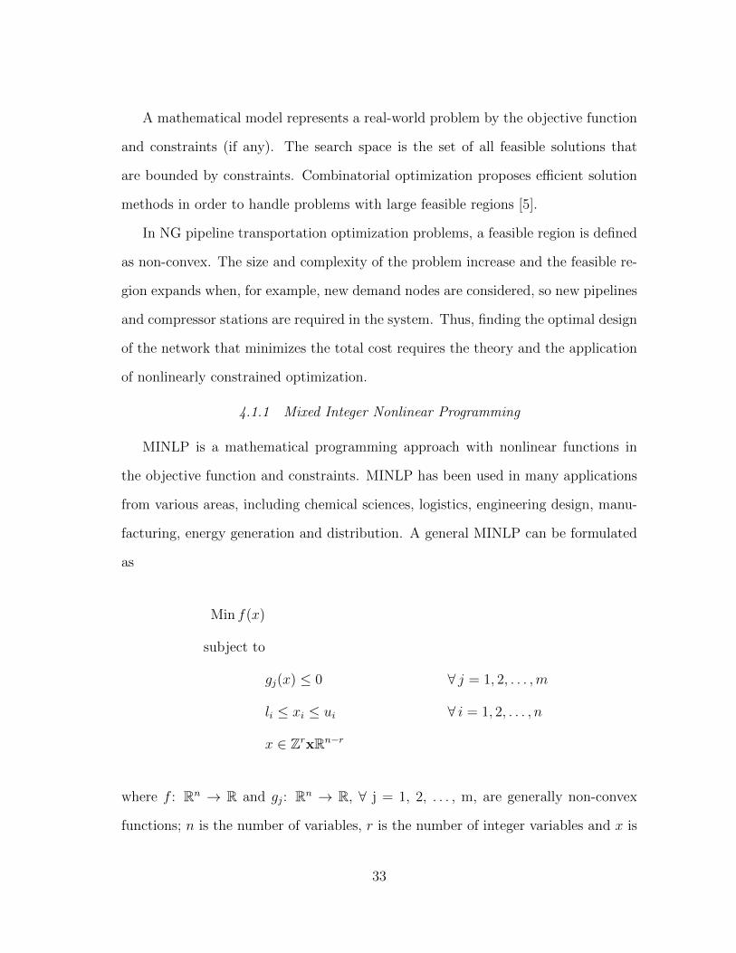
4.1.1 Mixed Integer Nonlinear Programming
MINLP is a mathematical programming approach with nonlinear functions in
the objective function and constraints. MINLP has been used in many applications
from various areas, including chemical sciences, logistics, engineering design, manu-
facturing, energy generation and distribution. A general MINLP can be formulated
as
Min f(x)
subject to
gj(x) ≤ 0 ∀ j = 1, 2, . . . ,m
li ≤ xi ≤ ui ∀ i = 1, 2, . . . , n
x ∈ ZrxRn−r
where f : Rn → R and gj: Rn → R, ∀ j = 1, 2, . . . , m, are generally non-convex
functions; n is the number of variables, r is the number of integer variables and x is
33

the n-vector of variables where li and ui determine lower and upper bounds on the
variables [3].
MINLP problems are very difficult to solve, because they include the difficulties
of both MIP and nonlinear programming (NLP), which are MINLP’s subclasses. As
MIP has a combinatorial nature, non-convex and convex NLP problems are hard to
solve. Since both MIP and NLP are NP-complete problems, solving MINLP can be
challenging.
Non-convex MINLPs are typically harder to solve optimally than convex prob-
lems. For convex MINLPs, an initial lower bound can be computed by solving the
continuous relaxation of the problem. This relaxation will be a convex NLP so that it
is relatively easy to solve. On the other hand, a continuous relaxation of a non-convex
MINLP is a non-convex NLP, which is classified as a NP-hard problem. [3]
Defining a NG transmission network requires using nonlinear equalities and bi-
nary variables. Therefore, MINLP is used to describe the problem. Because of the
characteristics of the pressure and flow rate relation, the feasible region of the prob-
lem is non-convex. Typically, the BB algorithm is used to solve nonlinear non-convex
problems.
4.1.2 The Branch-and-Bound Algorithm
Bonmin solves non-convex MINLP problems using BB algorithm. This algorithm
is the method for global optimization in non-convex problems [17]. The method is to
branch on all variables before closing the gap between the lower and upper bound on
the globally optimal objective value. These algorithms can be slow. In some cases
computational times increase exponentially with problem size [7].
The space of all feasible solutions (the search space) is repeatedly partitioned
into submodels. After tightening the bounds on the discrete variables to integer
34

values, non-integer solutions are eliminated. A tightened submodel is solved by using
the optimal solution to the previous looser submodel. In the case of minimization,
the objective function values of submodels are assumed to be lower bounds in the
restricted search space. The search continues to examine further nodes in the tree
until a feasible solution with an objective function value that is no greater than the
bound for any submodel [27].
For constrained optimization problems with discrete variables and/or non-convex
objective function or constraints, exact solution methods are inefficient. BB methods
are one of the best ways to obtain globally optimal solutions to nonlinear program-
ming problems with non-convex functions [17].
4.1.3 Overview of AMPL and Bonmin
Modeling language systems are widely used tools in the development of math-
ematical models. One of the most widely used modeling languages is AMPL [12].
AMPL is an algebraic modeling language for formulating and solving high-complexity
problems for a large-scale mathematical computation. Linear and nonlinear opti-
mization problems with discrete or continuous variables can be modeled by AMPL.
AMPL’s syntax is similar to mathematical notations of optimization problems. This
allows for a comprehensible definition of models. In this study, AMPL is used to
describe the problem model.
AMPL solver options comprise a considerable number of optimization tools in-
cluding, CPLEX[16], Gurobi[14], MINOS[21], and KNITRO[7] . The solvers differ
from each other in such a way that each apply different methods to solve problems
with a given proven optimality and the characteristics of the models they handle.
After modeling with AMPL, the problem will be solved by Bonmin (Basic Open-
source Nonlinear Mixed Integer Programming) [4]. The aim is to assess the com-
35
putability of the model. Bonmin is an online solver of the Computational Infras-
tructure for Operations Research (COIN-OR) [18], which is an initiative project to
encourage the development of open-source software for the operations research com-
munity. Bonmin and many other COIN-OR solvers can be accessed on-line through
the NEOS Server [10]. Optimization problems are solved by solvers automatically
with minimal input from the user. Users upload the problem’s formulation to the
server as an input. AMPL, GAMS[25] or MATLAB[19] can be used to define prob-
lems. All other information required by the optimization solver is determined au-
tomatically. For each problem type, there are different optimization solvers. For
instance, BARON[26], Bonmin or Couenne[2] can be used to solve MINLP.
Bonmin is an open source code for solving general MINLP problems in AMPL ,
GAMS and C/C++ format. The methods that Bonmin uses exact algorithms when
nonlinear functions are convex. Bonmin implements four different algorithms for
solving MINLPs: (1) a NLP-based BB algorithm, (2) an outer-approximation based
BB algorithm, (3) an outer-approximation based decomposition algorithm, and (4)
a hybrid outer-approximation/NLP based branch-and-cut algorithm. A NLP-based
BB algorithm solves a continuous nonlinear program at each node of the search tree
and branches on variables [4].
4.2 Computational Study and Analysis
In this section, an evaluation of the computability of the proposed model is pro-
vided. The network problems are generated by using the assumptions and the pa-
rameters that were discussed previously. Different variations of the model are tested.
Outputs of the problems are compared, and the robustness of solutions is discussed.
Input data are realistic data, i.e., demand quantities are randomly generated
according to the current usage in Turkey by using uniform distribution. Then, using
36
these data, monthly, seasonal and yearly data were computed. Monthly demands
vary in each period according to the season. For instance, peak demand occurs in
the winter session between October and March. Summer session is between April
and September. This season holds the lowest demand in a year. Seasonal demands
are the summation of demands in a season while yearly demand is the total of the
two seasons’ demand values. Typically, demand increases over 5 years between 5%
and 15%. In this study, it is assumed that demand increases by 1% in each year.
The structure of the studied networks is inspired by the transmission network of
Turkey. The position of nodes is consistent with their geographical location in the
real network.
Flow directions are designated by the constraints and no flow direction is assigned
a priori. The length and diameter of pipeline arcs are established before running the
test instances. The pressure of gas at supply nodes is fixed to 75 bar. The pressure at
other nodes is limited by the maximum allowable operating pressure of the pipeline.
The operating pressures of the pipelines are not given as problem data, but they are
computed during the optimization run by satisfying constraints.
As a result of numerical experiments, the model is expected to have a tree-
structured network that there is at least one path to any demand node and at least
one path from any supply node. It is also anticipated that all demand and capacity
requirements are satisfied in all periods, and pressures at nodes are in the allowed
range. Once a pipeline or a compressor station is installed, the model will adjust gas
flow accordingly in latter periods.
The following data has been decided to be used due to the evidence suggested by
many test instances. Length and resistance of each pipe type are given in Table 4.1
and demand data are shown in Table 4.2.
37

Table 4.1: Monthly Demand Data (mmscm)Demand Periods
Nodes JAN FEB MAR APR MAY JUN JUL AUG SEP OCT NOV DEC
2 158.98 144.53 98.71 81.58 74.16 67.42 61.29 55.72 89.74 108.58 119.44 131.39
3 163.28 148.43 101.38 83.79 76.17 69.25 62.95 57.23 92.17 111.52 122.67 134.94
5 139.83 127.12 86.82 71.75 65.23 59.30 53.91 49.01 78.93 95.50 105.05 115.56
6 141.37 128.52 87.78 72.55 65.95 59.96 54.50 49.55 79.80 96.56 106.21 116.84
8 114.59 104.17 71.15 58.80 53.46 48.60 44.18 40.16 64.68 78.27 86.09 94.70
9 116.03 105.48 72.04 59.54 54.13 49.21 44.73 40.67 65.50 79.25 87.17 95.89
10 176.96 160.87 109.88 90.81 82.55 75.05 68.23 62.02 99.89 120.87 132.95 146.25
12 87.58 79.62 54.38 44.94 40.86 37.14 33.77 30.70 49.44 59.82 65.80 72.38
17 115.34 104.86 71.62 59.19 53.81 48.92 44.47 40.43 65.11 78.78 86.66 95.32
18 176.88 160.80 109.83 90.77 82.51 75.01 68.19 61.99 99.84 120.81 132.89 146.18
19 132.47 120.43 82.25 67.98 61.80 56.18 51.07 46.43 74.78 90.48 99.53 109.48
20 147.66 134.23 91.68 75.77 68.88 62.62 56.93 51.75 83.35 100.85 110.94 122.03
22 158.24 143.86 98.26 81.20 73.82 67.11 61.01 55.46 89.32 108.08 118.89 130.78
25 84.91 77.19 52.72 43.57 39.61 36.01 32.74 29.76 47.93 57.99 63.79 70.17
26 176.89 160.81 109.83 90.77 82.52 75.02 68.20 62.00 99.85 120.82 132.90 146.19
30 113.34 103.03 70.37 58.16 52.87 48.07 43.70 39.72 63.98 77.41 85.15 93.67
31 131.88 119.89 81.89 67.67 61.52 55.93 50.84 46.22 74.44 90.07 99.08 108.99
33 160.04 145.49 99.37 82.13 74.66 67.87 61.70 56.09 90.34 109.31 120.24 132.26
35 71.84 65.31 44.61 36.86 33.51 30.47 27.70 25.18 40.55 49.07 53.97 59.37
37 71.39 64.90 44.33 36.64 33.31 30.28 27.53 25.02 40.30 48.76 53.64 59.00
39 63.28 57.52 39.29 32.47 29.52 26.83 24.40 22.18 35.72 43.22 47.54 52.29
40 71.25 64.77 44.24 36.56 33.24 30.22 27.47 24.97 40.22 48.67 53.53 58.89
42 109.69 99.72 68.11 56.29 51.17 46.52 42.29 38.44 61.92 74.92 82.41 90.65
44 180.11 163.74 111.84 92.43 84.02 76.39 69.44 63.13 101.67 123.02 135.32 148.85
46 135.71 123.37 84.27 69.64 63.31 57.56 52.32 47.57 76.61 92.69 101.96 112.16
48 114.45 104.05 71.06 58.73 53.39 48.54 44.13 40.11 64.60 78.17 85.99 94.59
49 132.29 120.26 82.14 67.88 61.71 56.10 51.00 46.37 74.67 90.35 99.39 109.33
50 186.19 169.27 115.61 95.55 86.86 78.96 71.79 65.26 105.10 127.17 139.89 153.88
52 129.62 117.83 80.48 66.51 60.47 54.97 49.97 45.43 73.17 88.53 97.38 107.12
55 53.42 48.56 33.17 27.41 24.92 22.65 20.59 18.72 30.15 36.48 40.13 44.15
58 186.71 169.74 115.93 95.81 87.10 79.18 71.98 65.44 105.39 127.53 140.28 154.31
59 121.83 110.75 75.65 62.52 56.83 51.67 46.97 42.70 68.77 83.21 91.53 100.69
60 70.11 63.73 43.53 35.98 32.71 29.73 27.03 24.57 39.57 47.88 52.67 57.94
62 172.63 156.93 107.19 88.58 80.53 73.21 66.55 60.50 97.44 117.91 129.70 142.67
63 175.19 159.26 108.78 89.90 81.73 74.30 67.54 61.40 98.89 119.66 131.62 144.78
66 135.11 122.83 83.89 69.33 63.03 57.30 52.09 47.36 76.27 92.28 101.51 111.66
68 77.57 70.52 48.16 39.80 36.19 32.90 29.91 27.19 43.78 52.98 58.28 64.10
69 177.22 161.11 110.04 90.94 82.67 75.16 68.32 62.11 100.03 121.04 133.14 146.46
71 76.51 69.55 47.50 39.26 35.69 32.45 29.50 26.82 43.19 52.26 57.48 63.23
73 93.12 84.66 57.82 47.79 43.44 39.49 35.90 32.64 52.56 63.60 69.96 76.96
79 62.65 56.96 38.90 32.15 29.23 26.57 24.16 21.96 35.37 42.79 47.07 51.78
81 76.31 69.37 47.38 39.16 35.60 32.36 29.42 26.74 43.07 52.12 57.33 63.06
82 71.96 65.42 44.68 36.93 33.57 30.52 27.74 25.22 40.62 49.15 54.07 59.47
83 160.80 146.19 99.85 82.52 75.02 68.20 62.00 56.36 90.77 109.83 120.81 132.90
85 43.71 39.74 27.14 22.43 20.39 18.54 16.85 15.32 24.68 29.86 32.84 36.13
87 53.32 48.47 33.11 27.36 24.87 22.61 20.56 18.69 30.10 36.42 40.06 44.07
88 155.78 141.62 96.73 79.94 72.67 66.07 60.06 54.60 87.93 106.40 117.04 128.74
90 112.56 102.33 69.89 57.76 52.51 47.74 43.40 39.45 63.54 76.88 84.57 93.03
38

Table 4.2: Pipeline Arc Lengths and ResistancesArc φij (km) δij Arc φij (km) δij Arc φij (km) δij
1,2 25 1.344 38,40 5 0.269 72,73 10 0.537
2,3 25 1.344 38,39 20 1.075 72,74 100 5.374
3,4 25 1.344 34,41 50 2.687 74,75 50 2.687
4,5 30 1.612 41,42 45 2.418 75,76 10 0.537
5,6 30 1.612 43,44 5 0.269 75,85 50 2.687
6,7 30 1.612 43,45 50 2.687 85,86 5 0.269
7,9 60 3.225 45,46 45 2.418 86,87 10 0.537
7,8 30 1.612 45,47 50 2.687 86,88 5 0.269
9,10 60 3.225 47,48 75 4.031 77,78 10 0.537
4,11 50 2.687 48,49 75 4.031 78,79 5 0.269
11,12 5 0.269 47,50 50 2.687 78,80 25 1.344
11,13 50 2.687 29,51 100 5.374 80,81 20 1.075
14,15 50 2.687 51,52 5 0.269 80,82 20 1.075
15,16 40 2.150 51,53 50 2.687 80,83 25 1.344
16,19 20 1.075 53,54 25 1.344 83,84 50 2.687
16,17 20 1.075 54,55 5 0.269 89,90 10 0.537
16,18 20 1.075 54,56 25 1.344 74,89 10 0.537
19,20 20 1.075 56,57 20 1.075 41,91 25 1.344
15,21 50 2.687 57,58 20 1.075 43,92 25 1.344
21,22 5 0.269 57,59 20 1.075 31,93 25 1.344
21,23 50 2.687 56,60 50 2.687 32,94 25 1.344
23,24 50 2.687 50,61 50 2.687 18,20 20 1.075
24,25 10 0.537 60,62 60 3.225 25,26 20 1.075
24,26 10 0.537 60,63 60 3.225 33,39 20 1.075
23,27 50 2.687 60,96 50 2.687 37,42 20 1.075
28,29 50 2.687 64,97 50 2.687 42,46 20 1.075
29,30 5 0.269 64,65 100 5.374 55,58 20 1.075
29,31 50 2.687 65,66 5 0.269 17,26 50 2.687
32,34 50 2.687 65,67 75 4.031 17,18 30 1.612
32,33 5 0.269 67,68 50 2.687 79,88 50 2.687
34,35 10 0.537 68,69 100 5.374 79,81 30 1.612
35,36 10 0.537 67,70 75 4.031 59,63 20 1.075
36,38 100 5.374 70,71 5 0.269 70,95 50 2.687
36,37 5 0.269 53,72 5 0.269
39
The investment costs of pipeline and compressor station installations will be de-
creasing in each year due to straight line depreciation method. For example, the
investment cost of a compressor station in the first year is not the same as the in-
vestment cost in the second year. Moreover, the operating costs of pipelines decrease
while compressor station operating costs increase in each year. Transportation cost
also varies depending on the total costs of compressor station and pipelines. Since
gas prices increase 2% each year, purchase cost changes in each period.
The numerical examples were solved in less than 8 hours with an allowable gap
of 5%. However, all solutions are obtained with an integer gap less than 0%.
4.2.1 Experiment 1: Various Problem Sizes
In this experiment, the computational performance of the proposed model is ex-
amined by different problem sizes. The subjects of the experiment are three realistic
different transmission networks, one with 31, the other with 66 and another with 97
nodes. Output of each test instance provides information about the design of the
network, the location of pipeline and compressor station installations, the amount of
gas that should be purchased at the beginning of the period.
The pipeline lengths in both networks vary from 5 km to 100 km and the diameter
of each pipeline is 30 inches. The total pipeline length of the 31-node network is 1040
km, of the 66-node network is 2440 km, and of the 97-node network is 3500 km.
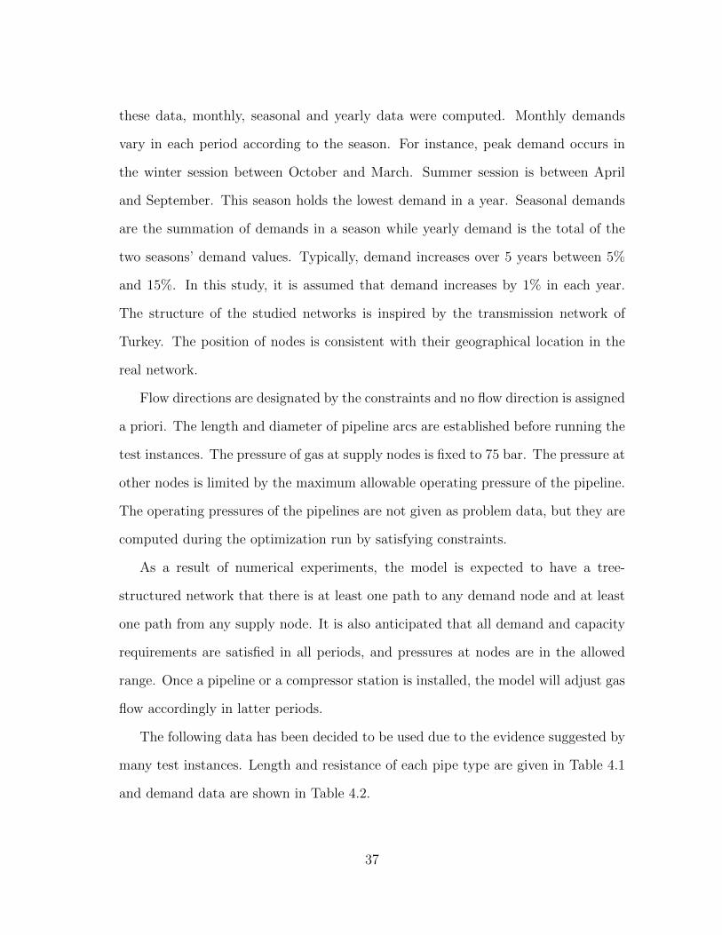
31-node problem network has 32 pipe arcs, and 2 compressor arcs. The system
was constituted with 2 supply, 16 demand, 9 transshipment nodes, and 2 compressor
stations. Figure 4.1 shows the underlying network of the problem. The mathematical
formulation of this network for one period has 181 binary, 149 continuous variables,
as well as 140 nonlinear, 403 linear, 105 equality, and 438 inequality constraints.
40
3
2
4
65
7 8
11
9
10
12
15
16
19
2018
17
21
22
23
24
2526
29
30
31
1
13142728
Figure 4.1: A Network with 31 Nodes
1
3
2
4
65
7 8
11
9
10
12
131415
16
19
2018
17
21
22
23
24
2526
272829
30
31
t=1
u=1
Figure 4.2: Solution to the 31-Node Network for 1-period
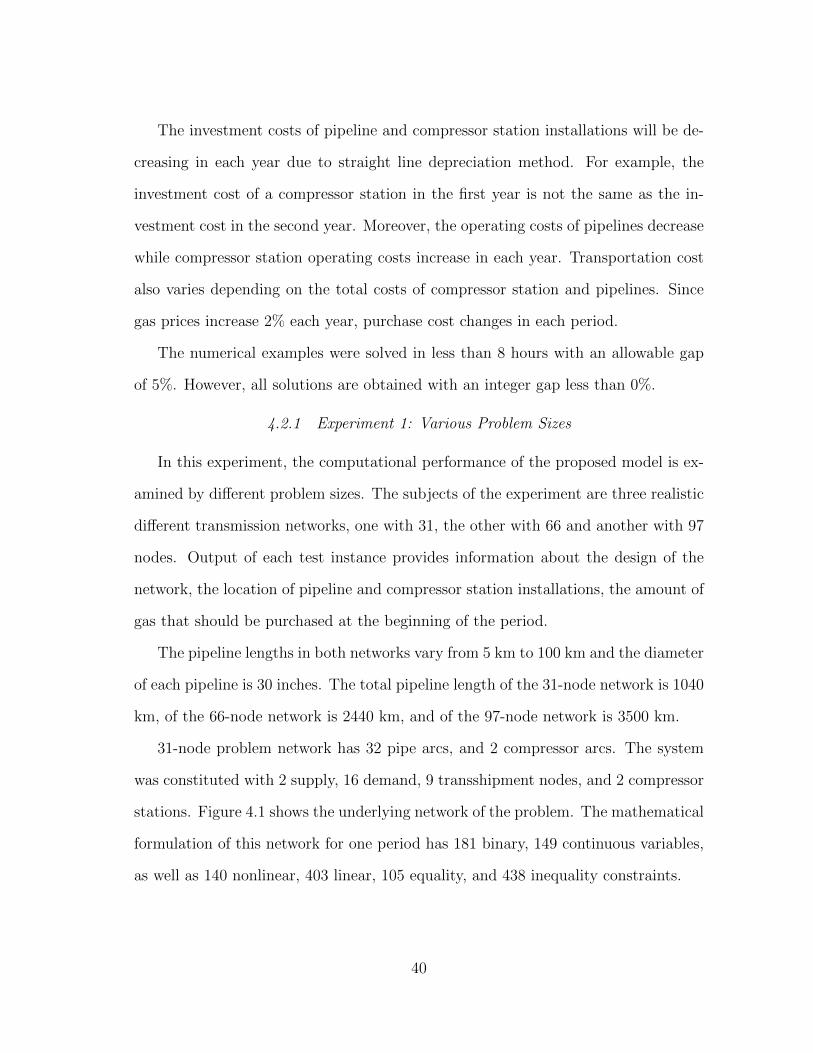
As shown in Figure 4.2, the output of the problem with one period consists of
two tree networks, and there is at least one path to each demand node. Compressor
stations at nodes 13-14 and 27-28 are installed and they will be available during 12
41

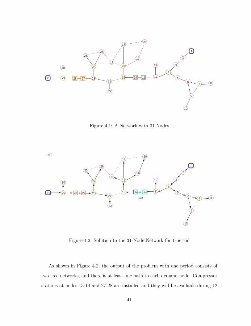
years. Pressures at nodes are given in Table 4.3 and Figure 4.3 shows the daily flow
rate in the period.
Table 4.3: Pressure Levels at Nodes in the 31-Node Network for 1-periodNode Pressure (bar) Node Pressure (bar)
1 75.00 17 71.19
2 62.81 18 70.79
3 50.86 19 71.12
4 39.03 20 70.70
5 33.74 21 72.36
6 29.91 22 72.33
7 29.73 23 72.59
8 29.55 24 71.41
9 27.49 25 71.39
10 26.55 26 71.27
11 33.01 27 75.00
12 32.99 28 68.84
13 27.93 29 71.38
14 75.00 30 71.36
15 72.91 31 75.00
16 71.19
As shown in the Table 4.3, while gas flows, pressure drops because of the resistance
and flow losses. Even though the pressure at the node 28 is above 45 bar, compressor
station is installed at that node in order to balance the pressure drop and flow rate.
Furthermore, at some nodes pressure is below 45 bar, so system analysts can decide to
locate compressor stations at other nodes considering cost and geotechnical factors.
As shown in Figure 4.3, at least 49.41 mmscm gas must be delivered from suppliers
in a year; 35.36 mmscm from supplier 1, and 14.05 mmscm from supplier 2.
42
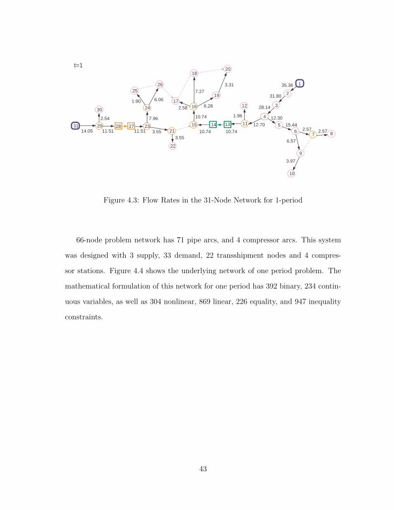
1
3
2
4
65
7 8
11
9
10
12
131415
16
19
2018
17
21
22
23
24
2526
272829
30
31
t=1
35.36
31.80
28.14
15.44
12.30
2.57 2.57
6.57
12.70
3.97
1.96
10.7410.74
10.74
2.58
7.27
6.28
3.31
3.553.55
7.96
1.90 6.06
11.51 11.51
2.54
14.05
Figure 4.3: Flow Rates in the 31-Node Network for 1-period
66-node problem network has 71 pipe arcs, and 4 compressor arcs. This system
was designed with 3 supply, 33 demand, 22 transshipment nodes and 4 compres-
sor stations. Figure 4.4 shows the underlying network of one period problem. The
mathematical formulation of this network for one period has 392 binary, 234 contin-
uous variables, as well as 304 nonlinear, 869 linear, 226 equality, and 947 inequality
constraints.
43

3
2
4
65
7 8
11
9
10
12
15
16
19
2018
17
21
22
23
24
2526
272829
30
5153
61
54
5552
5856
60
57
59
31
64
65
32 33 39
38 40
36
35
34
41
42
37
62
63
43
44
45 46
47
5049 48
65
1
1314
Figure 4.4: A Network with 66 Nodes
44

3
2
4
65
7 8
11
9
10
12
15
16
19
2018
17
21
22
23
24
2526
272829
30
5153
61
54
5552
5856
60
57
59
31
64
65
32 33 39
38 40
36
35
34
41
42
37
62
63
43
44
45 46
47
5049 48
u=2 u=2
u=1
u=2
1
1314
t=1
66
Figure 4.5: Solution to the 66-Node Network for 1-period
As shown in Figure 4.5, the problem solution consists of two tree networks, and
there is at least one path to each demand node. Compressor stations are needed at
each compressor station node during the period.
97-node problem network has 102 pipe arcs, and 6 compressor arcs. This system
was designed with 4 supply, 48 demand, and 33 transshipment nodes. Figure 4.6
shows the underlying network of one period problem. The mathematical formulation
of this network for one period has 563 binary, 340 continuous variables, as well as
436 nonlinear, 1252 linear, 328 equality, and 1360 inequality constraints.
45
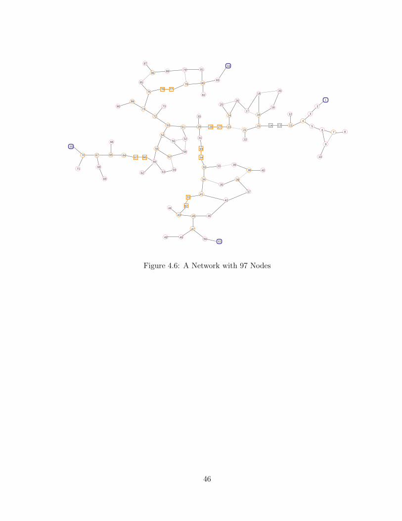
3
2
4
65
7 8
11
9
10
12
15
16
19
2018
17
21
22
23
24
2526
272829
30
5153
72
54
5552
5856
60
57
59
31
93
94
32 33 39
38 40
36
35
34
41
42
37
91
92
43
44
45 46
47
5049 48
1
1314
61
7374
89
90
6362
6465
66
67
68
69
70
71
95
9697
75
85
8688
87
7776
78
79 81
80
82
83
84
Figure 4.6: A Network with 97 Nodes
46

3
2
4
65
7 8
11
9
10
12
15
16
19
2018
17
21
22
23
24
2526
272829
30
5153
72
54
5552
5856
60
57
59
31
93
94
32 33 39
38 40
36
35
34
41
42
37
91
92
43
44
45 46
47
5049 48
u=2
u=2
1
1314
t=1
61
7374
89
90
6362
6465
66
67
68
69
70
71
95
u=2
9697
75
85
8688
87
7776
u=1
78
79 81
80
82
83
84
Figure 4.7: Solution to the 97-Node Network for 1-period
Figure 4.7, the problem solution consists of two tree networks, and there is at
least one path to each demand node. 4 compressor stations at nodes 13-14, 76-77,
93-94, and 96-97, are installed in the system. Gas is supplied from all suppliers.
Previous test instances showed that for larger size problems the computational
time exceeds 8 hours. Since they have more arcs and nodes, the model tries every arc
to minimize the total flow and cost. Therefore, the 66-node and 97-node problems
are solved for 1-period.
The optimal total cost and the solution time (CPU time) of each problem instance
are given in Table 4.4.
47

Table 4.4: Optimal Costs and Solution Times for Different Sized Networks
Problem Best objective value ($) CPU time (sec) Gap %
31-node 82,140,847,000 47.37 0.0013
66-node 163,811,060,000 258.41 0.00276
97-node 339,252,770,000 709.80 0.016
As presented in the Table 4.4, the optimal solution to the single period with
various network sizes can be obtained in less than one hour. However, the computa-
tional time increases with the number of nodes and arcs. Therefore, for the large size
problems, the whole network can be divided into small networks and each network
can be solved individually.
4.2.2 Experiment 2: The Effect of the Period Lengths
In this experiment, the model performance with different number of periods is
examined. The aim of this test study is to find the optimum planning horizon
length for the NG transmission network with varying levels of demand. The optimal
planning horizon not the only gives the minimum cost but also requires fewer changes
over 12 year span. System analysts try to operate the existing network structure
with minimal changes over long periods, because installing new pipelines/compressor
stations, and not using the existing ones, may cause considerable expenses.
Typically, demand projections, and compressor station and pipeline installation
decisions are made for 10 years. In this study, a 12 year span is chosen as a long term
planning horizon considering solution times of problems. It is also an appropriate
time period to observe changes on the network structure. Thus, various instances
based on the 31-node network are generated for different number of periods, but with
the same planning horizon length of 12 years.
48

Figure 4.8: Problems with Different Period Lengths
Figure 4.8 shows how these problems are generated. Regardless of the period
lengths, the mathematical formulation remains the same, but data changes according
to the number of years in a period. As mentioned before, demand and cost data are
generated for each year in the planning horizon. Based on these data, yearly demands
are aggregated to obtain periodical demand in each problem. For example, for 1-
period problem, demand values of 12 years are combined while in 2-period problem,
demand data of the first period is the summation of the first 6 years’ demand values.
49
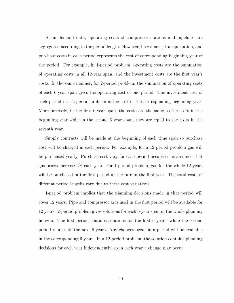
As in demand data, operating costs of compressor stations and pipelines are
aggregated according to the period length. However, investment, transportation, and
purchase costs in each period represents the cost of corresponding beginning year of
the period. For example, in 1-period problem, operating costs are the summation
of operating costs in all 12-year span, and the investment costs are the first year’s
costs. In the same manner, for 2-period problem, the summation of operating costs
of each 6-year span gives the operating cost of one period. The investment cost of
each period in a 2-period problem is the cost in the corresponding beginning year.
More precisely, in the first 6-year span, the costs are the same as the costs in the
beginning year while in the second 6 year span, they are equal to the costs in the
seventh year.
Supply contracts will be made at the beginning of each time span so purchase
cost will be charged in each period. For example, for a 12 period problem gas will
be purchased yearly. Purchase cost vary for each period because it is assumed that
gas prices increase 2% each year. For 1-period problem, gas for the whole 12 years
will be purchased in the first period at the rate in the first year. The total costs of
different period lengths vary due to these cost variations.
1-period problem implies that the planning decisions made in that period will
cover 12 years. Pipe and compressor arcs used in the first period will be available for
12 years. 2-period problem gives solutions for each 6-year span in the whole planning
horizon. The first period contains solutions for the first 6 years, while the second
period represents the next 6 years. Any changes occur in a period will be available
in the corresponding 6 years. In a 12-period problem, the solution contains planning
decisions for each year independently, so in each year a change may occur.
50

1
3
2
4
65
7 8
11
9
10
12
131415
16
19
2018
17
21
22
23
24
2526
272829
30
31
t=1
u=1
Figure 4.9: Solution to the 1-Period Planning
The network structure that is shown in Figure 4.9 is the solution to the 1-period
problem. The network consists of two trees with 26 pipe arcs. The compressor
stations at the 13-14 nodes and 27-28 nodes are active. Pressure at the node 28 is
above 45 bar, but the model installs compressor station at that node in order to
balance the pressure drop and flow rate. The net present value of the network is
$82,140,847,000. This problem provides the maximum minimized cost because the
model does not allow any changes in 12 years. The current network will be available
for the whole planning horizon.
51

1
3
2
4
65
7 8
11
9
10
12
131415
16
19
2018
17
21
22
23
24
2526
272829
30
31
t=1
u=1
1
3
2
4
65
7 8
11
9
10
12
131415
16
19
2018
17
21
22
23
24
2526
272829
30
31
t=2
u=1u=1
Figure 4.10: Solution to the 2-Period Planning
The solution to the 2-period problem is shown in Figure 4.2.2 and Figure 4.10.
The network remains the same in two 6 year spans. In the first period, a compres-
sor station at nodes 13-14 will be installed, and it will be available for the whole
planning horizon. The network structure is the same as the solution to the 1-period
planning problem in the second period. Compressor station at nodes 27-28 will be
active starting from the second 6 year span. The cost is less for this 2-period problem
52
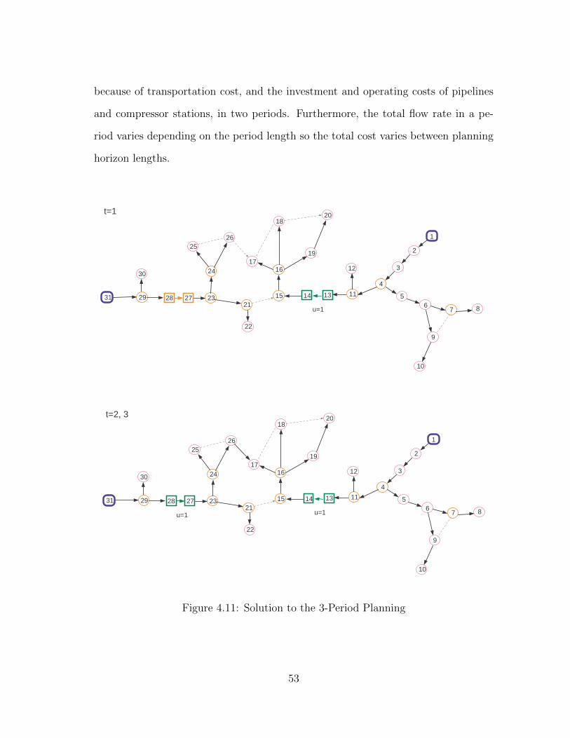
because of transportation cost, and the investment and operating costs of pipelines
and compressor stations, in two periods. Furthermore, the total flow rate in a pe-
riod varies depending on the period length so the total cost varies between planning
horizon lengths.
1
3
2
4
65
7 8
11
9
10
12
131415
16
19
2018
17
21
22
23
24
2526
272829
30
31
t=1
u=1
1
3
2
4
65
7 8
11
9
10
12
131415
16
19
2018
17
21
22
23
24
2526
272829
30
31
t=2, 3
u=1u=1
Figure 4.11: Solution to the 3-Period Planning
53

As shown in Figure 4.2.2 and Figure 4.11, for the first 4 year span of the 3-period
planning problem, the network structure is the same as the first periods of problems
with greater period length. For the last two periods, more precisely, in the last 8
years of the planning horizon, new pipeline and a compressor station at nodes 27-28
will be installed.
1
3
2
4
65
7 8
11
9
10
12
131415
16
19
2018
17
21
22
23
24
2526
272829
30
31
t=1, 2
u=1
1
3
2
4
65
7 8
11
9
10
12
131415
16
19
2018
17
21
22
23
24
2526
272829
30
31
t=3
u=1u=1
Figure 4.12: Solution to the 4-Period Planning (1)
54
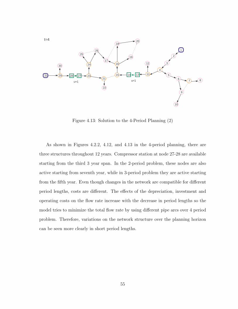
1
3
2
4
65
7 8
11
9
10
12
131415
16
19
2018
17
21
22
23
24
2526
272829
30
31
t=4
u=1u=1
Figure 4.13: Solution to the 4-Period Planning (2)
As shown in Figures 4.2.2, 4.12, and 4.13 in the 4-period planning, there are
three structures throughout 12 years. Compressor station at node 27-28 are available
starting from the third 3 year span. In the 2-period problem, these nodes are also
active starting from seventh year, while in 3-period problem they are active starting
from the fifth year. Even though changes in the network are compatible for different
period lengths, costs are different. The effects of the depreciation, investment and
operating costs on the flow rate increase with the decrease in period lengths so the
model tries to minimize the total flow rate by using different pipe arcs over 4 period
problem. Therefore, variations on the network structure over the planning horizon
can be seen more clearly in short period lengths.
55

1
3
2
4
65
7 8
11
9
10
12
131415
16
19
2018
17
21
22
23
24
2526
272829
30
31
t=1, 2, 3
u=2
1
3
2
4
65
7 8
11
9
10
12
131415
16
19
2018
17
21
22
23
24
2526
272829
30
31
t=4, 5, 6
u=1u=2
Figure 4.14: Solution to the 6-Period Planning
Figure 4.2.2 and Figure 4.14 represent the solution to the 6-period planning. The
network consists of only one tree and the compressor station at nodes 13-14 is active
while the one at nodes 27-28 is bypassed in the first 3 periods. As in the previous
problems, both compressor stations are active in the latter periods because of the
increasing demand. The model tries to keep the balance between the flow rate and
the pressure drop. Therefore, in the last 3 periods, the model requires installation of
56

a compressor station at nodes 27-28 starting from the seventh year to increase the
pressure. As in the previous problems, there are two pipe arcs that deliver gas to
node 17. To minimize the total flow, the model installs new pipeline from node 26
to node 17. Thus, both the flow rate and the cost is minimized.
1
3
2
4
65
7 8
11
9
10
12
131415
16
19
2018
17
21
22
23
24
2526
272829
30
31
t=1, 2, 3, 4, 5, 6
u=2
1
3
2
4
65
7 8
11
9
10
12
131415
16
19
2018
17
21
22
23
24
2526
272829
30
31
t=7, 8, 9, 10, 11, 12
u=2u=1
Figure 4.15: Solution to the 12-Period Planning
57
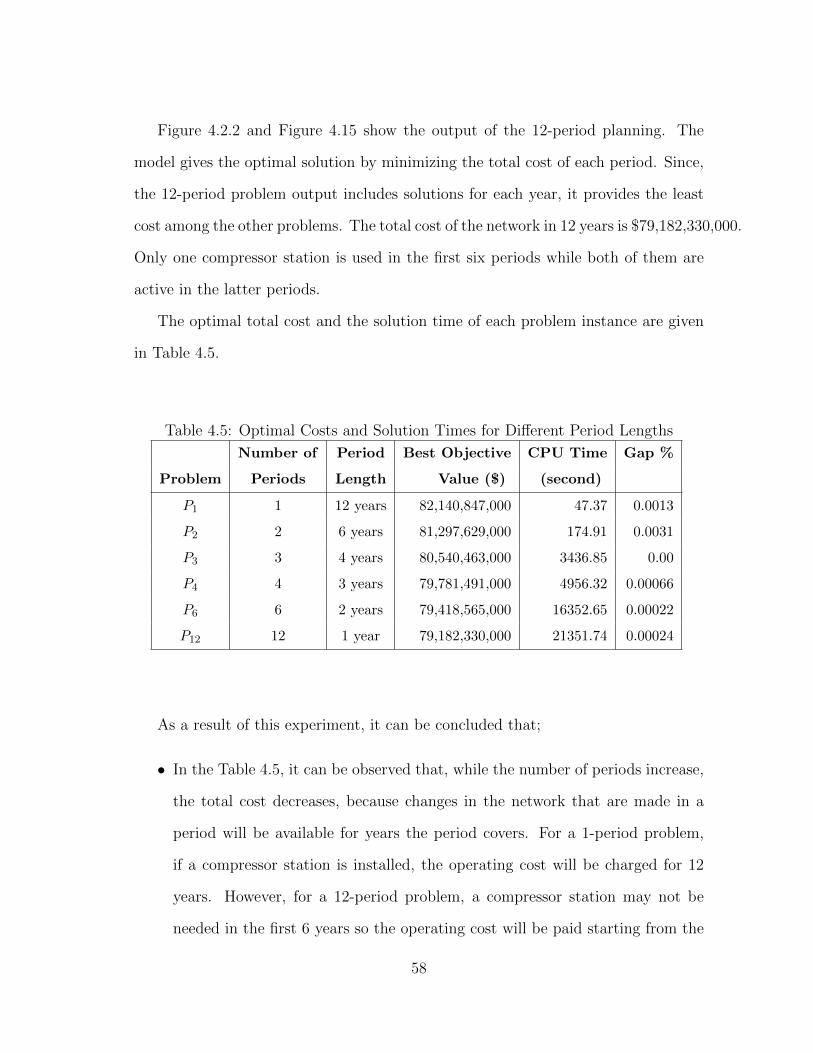
Figure 4.2.2 and Figure 4.15 show the output of the 12-period planning. The
model gives the optimal solution by minimizing the total cost of each period. Since,
the 12-period problem output includes solutions for each year, it provides the least
cost among the other problems. The total cost of the network in 12 years is $79,182,330,000.
Only one compressor station is used in the first six periods while both of them are
active in the latter periods.
The optimal total cost and the solution time of each problem instance are given
in Table 4.5.
Table 4.5: Optimal Costs and Solution Times for Different Period Lengths
Number of Period Best Objective CPU Time Gap %
Problem Periods Length Value ($) (second)
P1 1 12 years 82,140,847,000 47.37 0.0013
P2 2 6 years 81,297,629,000 174.91 0.0031
P3 3 4 years 80,540,463,000 3436.85 0.00
P4 4 3 years 79,781,491,000 4956.32 0.00066
P6 6 2 years 79,418,565,000 16352.65 0.00022
P12 12 1 year 79,182,330,000 21351.74 0.00024
As a result of this experiment, it can be concluded that;
• In the Table 4.5, it can be observed that, while the number of periods increase,
the total cost decreases, because changes in the network that are made in a
period will be available for years the period covers. For a 1-period problem,
if a compressor station is installed, the operating cost will be charged for 12
years. However, for a 12-period problem, a compressor station may not be
needed in the first 6 years so the operating cost will be paid starting from the
58

seventh period. The operating cost for pipeline is also charged in the same
way. Therefore, solving each period individually helps with making the right
decisions in the right time.
• The key factor of the differences between the various planning horizons is the
strategy that is used to compute demand and cost for each one. For example,
for 6-period planning, it is assumed that demand values are the summation
of two consecutive years, while for 1-period planning demand values are the
summation of all yearly demands in 12 years. Demand values define the daily
flow rate in a pipeline. Since, demand values change in each year, daily flow
rates are also subject to change. Compressor stations are located at nodes
according to the pressure. Therefore, pressure values at nodes as well as the
location of compressor stations, are different in each year due to the changes
in daily flows. Moreover, since transportation and purchase costs depend on
the flow rate, the total cost also varies.
• Another factor is that the model allows changes in the network during long
time periods. For example, in 12-period planning, the network is allowed to
change during each of the 12 years to operate with the minimum cost. Thus,
the network changes after the sixth period. In the same manner, 4-period
planning gives 3 different network structure. The model makes changes on
the network to minimize the total cost. However, in 1-period planning, it is
assumed that the network will remain the same for 12 years as if it is in the
first period. On the other hand, the network structure may not be convenient
for the latter periods, so there can be sunk costs. Therefore, the cost increases
while the period length decreases.
59
• Demand values and cost data are crucial parameters for the NG network.
Therefore, the aggregate planning may not give reliable solutions to NG trans-
mission networks over long planning horizons.
• This study shows that planning each year independently from other years gives
more realistic solution with minimal costs. By using a multi-period planning
problem, compressor station and pipeline installation decisions can be made
more accurately.
In this experiment, it is shown that very similar network structure can be obtained
by using different period lengths for a planning horizon. The annual flow costs
implied by the problems, P1, P2, . . . , P12, of each scenario are compared to show
the robustness of the solution. To obtain associated flow cost for each problem,
transportation, and purchase costs are calculated for each year separately. The
network structures are fixed as obtained in each case and individual flow problems
are solved by using corresponding networks. Thus, it is assumed that these networks
are existing networks and they will be available as long as the period length of
a scenario. For example, for 1-period problem, network decisions for the whole
planning horizon are made only once at the beginning, so the network structure
remains the same during the whole planning horizon. The values of cost parameters,
which are transportation and purchase costs, of the first year are used for each year.
Since the cost data is the same in each year, the annual total cost varies over 12 years
according to the total flow. However, in 2-period problem, the network structure is
modified after sixth year, so the total flow changes. The cost parameter values also
vary in every two years due to gas prices or electricity costs. Therefore, yearly costs
vary over 12 years depending on both the cost and flow. Other problems Figure 4.16
shows the annual transportation and purchase costs of each problem.
60

Figure 4.16: Annual Costs of Different Period Lengths
As shown in Figure 4.16, for the first 7-year-span, the annual total costs of all
problems are very close to each other. Therefore, for a decision making process,
computational times of the problems must be considered. Consequently, 1-period
problem can be chosen, since it gives optimum results in a short time. However, the
total cost of the problem is not a minimum cost that can be obtained in 12 years.
The problem also assumes that there is not any change in the network structure
during planning horizon. Therefore, to obtain a realistic network structure and
modifications with a minimum cost, 12-period problem can be used.
For the rest of the planning horizon, the total costs vary depending on the period
lengths. As mentioned before, 1-period problem network structure does not change
during planning horizon, but demand increases over time. Therefore, even though
the cost parameter values are the same for all years, the total cost increases because
of the increase in flow. However, the output of the 12-period problem allows changes
61
in the network structure due to increasing demand. For example, if a pipeline is
needed in sixth year, 1-period problem may install it in the first year or it may not
consider it at all. The other problems that include more periods react the change in
time and adjust the network accordingly. Another advantage of 12-period planning
is the cost variation over planning horizon. The transporting cost of one mmscm of
gas decreases during 12 years while the total flow increases. Therefore, the total cost
is less than the total cost of 1-period problem. Thus, the difference between costs
increases over the last 5 years because of the cost variation in the problems.
The model can be run in different periods of time by using updated data. For
example, if new demand forecasts are available after sixth year, the model can be used
to optimize flow to find the minimum amount of gas purchase in the next periods.
Moreover, for existing networks, by fixing variables corresponding to pipeline and
compressor station arcs, expansion decisions, such as installing new pipelines or
compressor stations, can be made.
In summary, the operational and strategic plan for 12 years can be made at the
beginning of the planning horizon using a 1-period model structure, which has the
least computational time. However, since demand increases, the network may require
new pipelines and compressor stations over time; 1-period problem may not give
efficient solution for the next periods. 12-period problem gives reliable solutions, but
the computational time is more than the other problems. Consequently, considering
both the computational time and the output efficiency, the problems with 2, 3, 4 or
6 periods can be used. Thus, the model can be run in each period to make decisions
for the latter periods.
62

4.2.3 Experiment 3: The Effect of Changes in the Cost Parameters
In this experiment, the model performance with different cost parameters is ex-
amined. Another purpose of the study is to find the cost that affects the network
structure most. For this purpose, various test instances are generated for the 31-node
12-period network. The cost of investment and of operating compressor stations are
treated as one parameter. In the same manner, the total cost for pipelines consists
of the investment and operating costs. Also, the transportation cost is taken into
consideration to observe the changes in the network due to variable cost parameters.
Thus, the three costs used in the test runs are the total cost of compressor stations,
the total cost of pipelines, and the transportation cost. The upper and lower bounds
of the costs are computed by using 20% of each value. Smaller percentages of the cost
parameters did not affect the network remains the same in test runs of the model,
but for 20% and up the network structure changes.
The cost data that are used in these instances are shown in Table 4.6 and 4.7.
Test instances include different combinations of the lower and upper values of
costs. These combinations are shown as (I-II-III), where the first entry refers to
the transportation cost, the next one represents the total cost of pipelines and the
last one stands for the total cost of compressor stations. For example, (L-U-L)
implies that the problem has the lower values of transportation cost and the total
compressor station costs, and the upper value of the total pipeline cost. The best
objective function values and the solution times of instances are shown in Table 4.8.
63

Table 4.6: Cost Data (103 $) (1)Cost Period Actual Cost Lower Upper Cost Period Actual Cost Lower Upper
αct
1 10243.865 8195.092 12292.638
βct
1 24.709 19.7672 29.6508
2 9878.216 7902.5728 11853.8592 2 25.944 20.7552 31.1328
3 9459.014 7567.2112 11350.8168 3 27.242 21.7936 32.6904
4 8978.674 7182.9392 10774.4088 4 28.604 22.8832 34.3248
5 8428.558 6742.8464 10114.2696 5 30.034 24.0272 36.0408
6 7798.837 6239.0696 9358.6044 6 31.536 25.2288 37.8432
7 7078.328 5662.6624 8493.9936 7 33.112 26.4896 39.7344
8 6254.309 5003.4472 7505.1708 8 34.768 27.8144 41.7216
9 5312.313 4249.8504 6374.7756 9 36.506 29.2048 43.8072
10 4235.891 3388.7128 5083.0692 10 38.332 30.6656 45.9984
11 3006.347 2405.0776 3607.6164 11 40.248 32.1984 48.2976
12 1602.431 1281.9448 1922.9172 12 42.261 33.8088 50.7132
αpt
1 109.297 87.4376 131.1564
βpt
1 21.859 17.4872 26.2308
2 105.396 84.3168 126.4752 2 21.079 16.8632 25.2948
3 100.923 80.7384 121.1076 3 20.185 16.148 24.222
4 95.798 76.6384 114.9576 4 19.16 15.328 22.992
5 89.929 71.9432 107.9148 5 17.986 14.3888 21.5832
6 83.21 66.568 99.852 6 16.642 13.3136 19.9704
7 75.522 60.4176 90.6264 7 15.104 12.0832 18.1248
8 66.73 53.384 80.076 8 13.346 10.6768 16.0152
9 56.68 45.344 68.016 9 11.336 9.0688 13.6032
10 45.195 36.156 54.234 10 9.039 7.2312 10.8468
11 32.076 25.6608 38.4912 11 6.415 5.132 7.698
12 17.097 13.6776 20.5164 12 3.419 2.7352 4.1028
64

Table 4.7: Cost Data (103 $) (2)
Cost Period Actual Cost Lower Upper
βst
1 20.95 16.76 25.14
2 20.21 16.16 24.25
3 19.35 15.48 23.22
4 18.37 14.69 22.04
5 17.24 13.79 20.69
6 15.95 12.76 19.14
7 14.48 11.58 17.38
8 12.80 10.24 15.36
9 10.87 8.70 13.04
10 8.67 6.94 10.40
11 6.15 4.92 7.39
12 3.28 2.63 3.94
Table 4.8: Optimal Costs and Solution Times for Different Combinations of Cost
ParametersTest Best objective CPU time
Problem Instance value ($) (second) Gap %
T0 A-A-A 79,182,330,000 21351.74 0.00024
T1 L-L-L 77,488,495,000 21764.74 0.00189
T2 L-L-U 77,502,091,000 17187.34 0.00204
T3 L-U-L 77,576,231,000 22684.36 0.00258
T4 L-U-U 77,622,053,000 19981.68 0.00277
T5 U-L-L 80,253,805,000 19728.26 0.00354
T6 U-U-L 80,317,453,000 19628.51 0.00358
T7 U-L-U 80,336,401,000 19378.53 0.00439
T8 U-U-U 80,449,709,000 19609.75 0.00492
A: Actual cost / L: Lower value / U: Upper Value
65

Flow rate variables determine the design of the network. A pipeline is installed
between nodes i and j, if gas flows between these nodes. Therefore, the transporta-
tion cost that is related to the flow rate determines the network design. For the lower
values of the transportation cost, the network structure is the same as the original
12-period network. Different values of the total costs of compressor stations and
pipelines do not affect the network. As mentioned before, the model tries to find the
minimized total flow rate to reduce the costs. If transportation cost values are high,
the model searches for new paths to transport gas to keep the total flow rate at a
minimum so there are various structure throughout 12 years for each problem.
Figure 4.17 shows the solution to the problem with the upper values of transporta-
tion cost and the lower values of compressor station costs. The network remains the
same for the lower and upper values of pipeline costs. Figure 4.18 represent the prob-
lem output for the upper values of the transportation cost and compressor station
costs. This network is also the same for the different values of pipeline costs.
66
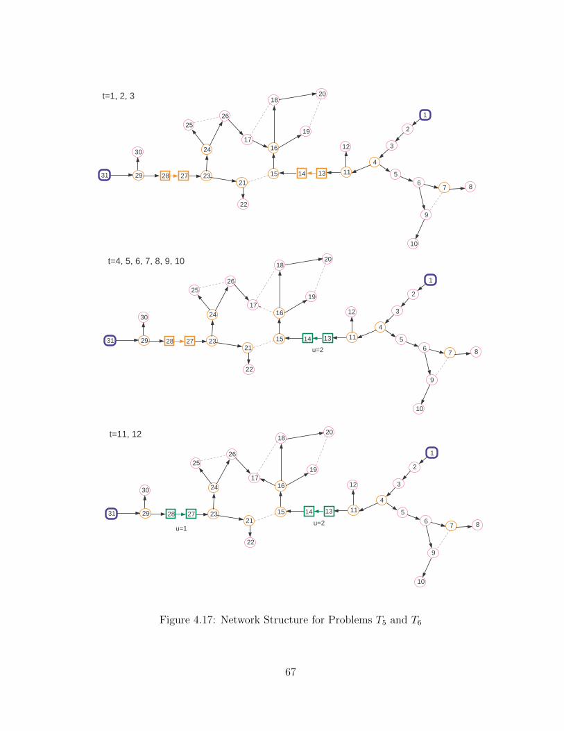
1
3
2
4
65
7 8
11
9
10
12
131415
16
19
2018
17
21
22
23
24
2526
272829
30
31
t=1, 2, 3
1
3
2
4
65
7 8
11
9
10
12
131415
16
19
2018
17
21
22
23
24
2526
272829
30
31
t=4, 5, 6, 7, 8, 9, 10
u=2
1
3
2
4
65
7 8
11
9
10
12
131415
16
19
2018
17
21
22
23
24
2526
272829
30
31
t=11, 12
u=2u=1
Figure 4.17: Network Structure for Problems T5 and T6
67
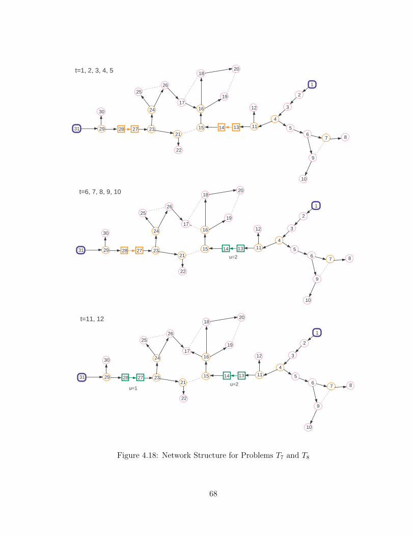
1
3
2
4
65
7 8
11
9
10
12
131415
16
19
2018
17
21
22
23
24
2526
272829
30
31
t=1, 2, 3, 4, 5
1
3
2
4
65
7 8
11
9
10
12
131415
16
19
2018
17
21
22
23
24
2526
272829
30
31
t=6, 7, 8, 9, 10
u=2
1
3
2
4
65
7 8
11
9
10
12
131415
16
19
2018
17
21
22
23
24
2526
272829
30
31
t=11, 12
u=2u=1
Figure 4.18: Network Structure for Problems T7 and T8
68
As shown in the Figure 4.17 and Figure 4.18, for the upper values of the trans-
portation cost, the network structure changes according to the total costs of com-
pressor stations. If the total cost of compressor stations is at the lower value then the
model installs a compressor station at nodes 13-14 starting from the fourth period.
If it is at the upper value then the station becomes active in the sixth period. The
costs of the pipeline do not change the structure.
In summary, it can be concluded that transportation cost is the most important
cost that affects the network structure. Decisions for choosing the best transportation
cost parameter must be made carefully. Too low or too high values can change the
network completely. Thus, the solution may not be applicable to the real-world
system. This study also showed that the model built with the upper values of
transportation cost and compressor stations tries to delay the installation decisions
for compressor stations. If installing compressor stations in the latter periods is
compatible with the other long-term plans, and the costs of the network are also
convenient for the company budget, then system analysts can use make decisions
accordingly. Since the model is cost sensitive, the scale between the cost parameters
is important. Costs must be calculated carefully to avoid getting any inapplicable
and costly results.
69
5. CONCLUSIONS AND FUTURE RESEARCH DIRECTIONS
This research addresses the problem of the optimization of a steady-state NG
transmission network. A MINLP model was proposed for minimizing the total in-
vestment and operating costs. The main contribution of this study is to provide
an integrated optimization model consisting of decision variables and constraints
that other researches studied before separately. The systematic design of various
test instances produced in this study assessed the proposed optimization approach,
when applied to different sized problems, in terms of efficiency and reliability. The
economic aspects of NG pipeline transportation were reviewed. Concepts of the in-
vestment cost of pipeline and compressor stations and the periodic operating costs
were introduced. The problem was modeled with AMPL. The numerical experiments
were conducted by application of a MINLP, Bonmin. This model will assist decision
makers to make appropriate decisions within a short time.
Flow networks have a complex structure in regard to gas characteristics and any
change or modification of their structure while in use is costly and difficult. Therefore,
designing a new network and utilizing of its capabilities optimally is important. In the
network model, arcs correspond to pipelines and compressor stations. The pipeline
flow and gas pressure at each node are the main decision variables in the problem. In
addition to flow conservation constraints, the model also includes a constraint that
defines the relationship of flow rate and pressure.
In the first type of test problems, the model was tested on three different networks
with 31, 66 and 97 nodes by using data for 1 period. In these problems, the actual
investment and operating costs were used. Demand parameters were representative of
the real-world system. Then, by generating different parameter settings, the changes
70
on the network structure were evaluated. For the second type of test problems,
the lengths of the periods were varied in order to detect the different modifications
that may occur in the system due to changes in the variables related to long-lasting
decisions. The robustness of the model output under varying scenarios was tested. In
the third type of test problems, discrete intervals for the cost parameter values were
used. The model was updated for each cost parameter value with different intervals
and the results were compared. The aim of this analysis is to assess the effect of cost
changes on the network structure as well as the run time of the problems. These
tests and analyses were applied on a small-size network with 31 nodes.
These test runs indicated that the proposed model gives effective results for multi-
period planning problems. The changes in the network structure can be observed,
and strategic and operational decisions can be made accordingly. The model pro-
vides solutions with minimized costs by reducing the total flow rate during a period.
This strategy requires fewer changes in the network over planning horizon. Since
compressor stations and pipelines are long-term investment decisions, system ana-
lysts try to maintain the same network for long years to avoid sunk costs. They also
try to minimize the number of idle pipelines and compressor stations in a period to
maximize the system efficiency. The solutions to the test instances showed that the
proposed model minimizes the total cost by making fewer changes on the network
for multi-period problems to satisfy increasing demand over planning horizon.
There are a couple of assumptions and limitations of this study. First, penalty
costs were not included in the study. In real-world problems, if the amount of
consumption is below the supply contract amount in a period, then the cost of
penalty must be paid for the excess amount of supply. Second, it is assumed that
there is no NG storages in the system. Gas is delivered only from different suppliers.
The first limitation may be overcome by introducing a new variable representing
71

the excess mount of supply. A new constraint may be defined to add the storage
to the system. The proposed model allows defining new variables and constraints
easily to enhance the interest area. In the operating perspective, there could be other
objective functions of interest such as minimizing the fuel consumption at compressor
stations.
In this study, optimization of design and operation of the steady-state natural gas
transmission systems were studied. Findings about the multi-purpose mathematical
model can be transferable to a wide range of research areas.
72
REFERENCES
[1] Arsegianto, A., E. Soewono, M. Apri. 2003. Non-linear optimization model for
gas transmission system: A case of grissik - duri pipeline. Asia Pacific Oil and
Gas Conference and Exhibition, Society of Petroleum Engineers.
[2] Belotti, P. 2006. COUENNE: a users manual. URL
http://www.coin-or.org/Couenne.
[3] Belotti, Pietro. 2012. Disjunctive cuts for nonconvex minlp. Mixed Integer Non-
linear Programming , The IMA Volumes in Mathematics and its Applications ,
vol. 154. Springer, New York, New York, 117–144.
[4] Bonami, P., J. Lee. 2011. Bonmin user’s manual. URL
http://www.coin-or.org/Bonmin.
[5] Borraz-Sanchez, C. Oct. 2010. Optimization methods for pipeline transforma-
tion of natural gas. Ph.D. Dissertation, University of Bergen, Norway .
[6] Borraz-Sanchez, C., R. Rios-Mercado. 2009. Improving the operation of pipeline
systems on cyclic structures by tabu search. Computers and Chemical Engineer-
ing 33 58–64.
[7] Boyd, S., A. Ghosh, A. Magnani. 2003. Branch and bound methods. URL Notes
for EE392o, Stanford University.
[8] Chebouba, A., F. Yalaoui, A. Smati, L. Amodeo, K. Younsi, A. Tairi. 2009. Op-
timization of natural gas pipeline transportation using ant colony optimization.
Computers& Operations Research 36 1916–1923.
73

[9] Chung, T.S., K.K. Li, G.J. Chen, J.D. Xie, G.Q. Tang. 2003. Multi-objective
transmission network planning by a hybrid ga approach with fuzzy decision
analysis. International Journal of Electrical Power & Energy Systems 25 187–
192.
[10] Czyzyk, J., M. Mesnier, J. More. 1998. The NEOS server. IEEE Journal on
Computational Science and Engineering 5 68–75.
[11] De Wolf, D., Y. Smeers. 2000. The gas transmission problem solved by extension
of the simplex algorithm. Management Science 46 1454–1465.
[12] Fourer, R., David M. Gay, Brian W. Kernighan. 2002. AMPL: A Modeling
Language for Mathematical Programming . Duxbury Press, Pacific Grove, Cali-
fornia.
[13] Hamedi, M., R.Z. Farahani, M.M. Husseini, G.R. Esmaeilian. 2009. A distribu-
tion planning model for natural gas supply chain: a case study. Energy Policy
37 799–812.
[14] Hamedi, M., R.Z. Farahani, M.M. Husseini, G.R. Esmaeilian. 2011. Optimiza-
tion in natural gas network planning. Logistics Operations and Management :
Concepts and Models - 393–420.
[15] Kabirian, A., M. R. Hemmati. 2007. A strategic planning model for natural gas
transmission networks. Energy Policy 35 5656–5670.
[16] Kennedy, John L. 1993. Oil and Gas Pipeline Fundamentals . PennWell Books,
Tulsa, Oklahoma.
[17] Lawler, E. L., D. E. Wood. 1966. Branch-and-bound methods: A survey. Oper-
ations Research 14 699–719.
74
[18] Lougee-Heimer, R. 2003. The common optimization interface for operations
research: Promoting open-source software in the operations research community.
IBM J. Res. Dev. 47 57–66.
[19] MATLAB. 2010. version 7.10.0 (R2010a). The MathWorks Inc., Natick, Mas-
sachusetts.
[20] Menon, Shashi E. 2005. Gas Pipeline Hydraulics . CRC Press, Boca Raton,
Florida.
[21] Osiadacz, A. J., D. J. Bell. 1986. A simplified algorithm for optimization of
large-scale gas networks. Optimal Control Applications and Methods 7 95–104.
[22] Pratt, K.F., J.G. Wilson. 1984. Optimization of the operation of gas transmis-
sion system. Transaction of the Instrument of the Measurement and Control 19
261–269.
[23] Rios-Mercado, R., S. Kim, E. Boyd. 2006. Efficient operation of natural gas
transmission systems: A network-based heuristic for cyclic structures. Comput-
ers & Operations Research 33 2323–2351.
[24] Rios-Mercado, Roger Z., S. Wu, L. Ridgway Scott, E. Andrew Boyd. 2001. A
reduction technique for ng transmission network optimization problems. Annals
Of Operations Research 117 217–234.
[25] Rosenthal, Richard E. 2012. GAMS: A user’s guide. URL
http://www.gams.com/.
[26] Sahinidis, N., M. Tawarmalani. 2011. BARON. URL
http://www.gams.com/dd/docs/solvers/baron.pdf.
75
[27] Tabkhi, F. Dec. 2007. Optimisation de reseaux de transport de gaz. Ph.D.
Dissertation, Institut National Polytechnique de Toulouse, France .
[28] Uraikul, V., C.W. Chan, P. Tontiwachwuthikul. 2003. MILP model for compres-
sor selection in natural gas pipeline operations. International Society for En-
vironmental Information Sciences, Environmental Informatics Archives 1 138–
145.
[29] US Department Of Energy, Energy Information Administration. 2009. Interna-
tional energy annual 2009. http://www.energy.gov .
[30] US Department Of Energy, Energy Information Administration. 2010. Interna-
tional energy annual 2010. http://www.energy.gov .
[31] Woldeyohannes, Abraham D., Mohd A. A. Majid. 2011. Simulation model for
natural gas transmission pipeline network system. Simulation Modelling Practice
and Theory 19 196–212.
[32] Wong, P. J., R. E. Larson. 1968. Optimization of tree-structured natural-gas
transmission networks. Journal of Mathematical Analysis and Applications 24
613–626.
[33] Wu, S., R.Z. Rios-Mercado, E.A. Boyd, L.R. Scott. 2000. Model relaxations for
the fuel cost minimization of steady-state gas pipeline networks. Mathematical
and Computer Modelling 31 197–200.
76