optimization (and learning)mlss.tuebingen.mpg.de › 2013 › 2013 › wright_slides.pdf ·...
TRANSCRIPT

Optimization (and Learning)
Steve Wright1
1Computer Sciences Department,University of Wisconsin,
Madison, WI, USA
MLSS, Tubingen, August 2013
S. J. Wright () Optimization MLSS, August 2013 1 / 158

Overview
Focus on optimization formulations and algorithms that are relevant tolearning.
Convex
Regularized
Incremental / stochastic
Coordinate descent
Constraints
Mention other optimization areas of potential interest, as time permits.
Mario Figueiredo (IST, Lisbon) collaborated with me on a tutorial onsparse optimization at ICCOPT last month. He wrote and edited many ofthese slides.
S. J. Wright () Optimization MLSS, August 2013 2 / 158
Matching Optimization Tools to Learning
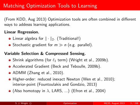
(From KDD, Aug 2013) Optimization tools are often combined in differentways to addesss learning applications.
Linear Regression.
Linear algebra for ‖ · ‖2. (Traditional!)
Stochastic gradient for m n (e.g. parallel).
Variable Selection & Compressed Sensing.
Shrink algorithms (for `1 term) (Wright et al., 2009b).
Accelerated Gradient (Beck and Teboulle, 2009b).
ADMM (Zhang et al., 2010).
Higher-order: reduced inexact Newton (Wen et al., 2010);interior-point (Fountoulakis and Gondzio, 2013)
(Also homotopy in λ, LARS, ...) (Efron et al., 2004)
S. J. Wright () Optimization MLSS, August 2013 3 / 158

Support Vector Machines.
Coordinate Descent (Platt, 1999; Chang and Lin, 2011).Stochastic gradient (Bottou and LeCun, 2004; Shalev-Shwartz et al.,2007).Higher-order methods (interior-point) (Ferris and Munson, 2002; Fineand Scheinberg, 2001); (on reduced space) (Joachims, 1999).Shrink Algorithms (Duchi and Singer, 2009; Xiao, 2010).Stochastic gradient + shrink + higher-order (Lee and Wright, 2012).
Logistic Regression (+ Regularization).
Shrink algorithms + reduced Newton (Shevade and Keerthi, 2003;Shi et al., 2008).Newton (Lin et al., 2008; Lee et al., 2006)Stochastic gradient (many!)Coordinate Descent (Meier et al., 2008)
Matrix Completion.
(Block) Coordinate Descent (Wen et al., 2012).Shrink (Cai et al., 2010a; Lee et al., 2010).Stochastic Gradient (Lee et al., 2010).
S. J. Wright () Optimization MLSS, August 2013 4 / 158
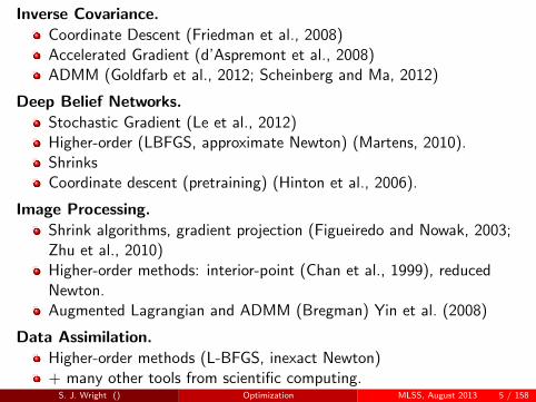
Inverse Covariance.
Coordinate Descent (Friedman et al., 2008)Accelerated Gradient (d’Aspremont et al., 2008)ADMM (Goldfarb et al., 2012; Scheinberg and Ma, 2012)
Deep Belief Networks.
Stochastic Gradient (Le et al., 2012)Higher-order (LBFGS, approximate Newton) (Martens, 2010).ShrinksCoordinate descent (pretraining) (Hinton et al., 2006).
Image Processing.
Shrink algorithms, gradient projection (Figueiredo and Nowak, 2003;Zhu et al., 2010)Higher-order methods: interior-point (Chan et al., 1999), reducedNewton.Augmented Lagrangian and ADMM (Bregman) Yin et al. (2008)
Data Assimilation.
Higher-order methods (L-BFGS, inexact Newton)+ many other tools from scientific computing.
S. J. Wright () Optimization MLSS, August 2013 5 / 158

1 First-Order Methods for Smooth Functions
2 Stochastic Gradient Methods
3 Higher-Order Methods
4 Sparse Optimization
5 Augmented Lagrangian Methods
6 Coordinate Descent
S. J. Wright () Optimization MLSS, August 2013 6 / 158

Just the Basics: Convex Sets
S. J. Wright () Optimization MLSS, August 2013 7 / 158

Convex Functions
S. J. Wright () Optimization MLSS, August 2013 8 / 158

Strong Convexity
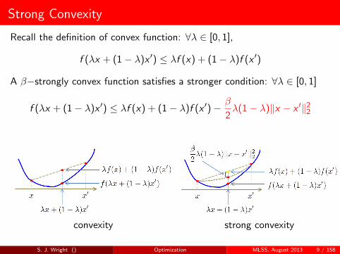
Recall the definition of convex function: ∀λ ∈ [0, 1],
f (λx + (1− λ)x ′) ≤ λf (x) + (1− λ)f (x ′)
A β−strongly convex function satisfies a stronger condition: ∀λ ∈ [0, 1]
f (λx + (1− λ)x ′) ≤ λf (x) + (1− λ)f (x ′)− β
2λ(1− λ)‖x − x ′‖2
2
convexity
strong convexity
S. J. Wright () Optimization MLSS, August 2013 9 / 158
Strong Convexity
Recall the definition of convex function: ∀λ ∈ [0, 1],
f (λx + (1− λ)x ′) ≤ λf (x) + (1− λ)f (x ′)
A β−strongly convex function satisfies a stronger condition: ∀λ ∈ [0, 1]
f (λx + (1− λ)x ′) ≤ λf (x) + (1− λ)f (x ′)− β
2λ(1− λ)‖x − x ′‖2
2
convexity strong convexity
S. J. Wright () Optimization MLSS, August 2013 9 / 158

A Little More on Convex Functions
Let f1, ..., fN : Rn → R be convex functions. Then
f : Rn → R, defined as f (x) = maxf1(x), ..., fN(x), is convex.
g : Rn → R, defined as g(x) = f1(L(x)), where L is affine, is convex.(“Affine” means that L has the form L(x) = Ax + b.)
h : Rn → R, defined as h(x) =∑N
j=1αj fj (x), for αj > 0, is convex.
An important function: the indicator of a set C ⊂ Rn,
ιC : Rn → R, ιC (x) =
0 ⇐ x ∈ C+∞ ⇐ x 6∈ C
If C is a closed convex set, ιC is a lower semicontinuous convex function.
S. J. Wright () Optimization MLSS, August 2013 10 / 158

Smooth Functions
Let f : Rn → R be twice differentiable and consider its Hessian matrix atx , denoted ∇2f (x).
[∇2f (x)]ij =∂f
∂xi∂xj, for i , j = 1, ..., n.
f is convex ⇔ its Hessian ∇2f (x) is positive semidefinite ∀x
f is strictly convex ⇐ its Hessian ∇2f (x) is positive definite ∀x
f is β-strongly convex ⇔ its Hessian ∇2f (x) βI , with β > 0, ∀x .
S. J. Wright () Optimization MLSS, August 2013 11 / 158

Norms: A Quick Review
Consider some real vector space V, for example, Rn or Rn×n, ...
Some function ‖ · ‖ : V → R is a norm if it satisfies:
‖αx‖ = |α| ‖x‖, for any x ∈ V and α ∈ R (homogeneity);
‖x + x ′‖ ≤ ‖x‖+ ‖x ′‖, for any x , x ′ ∈ V (triangle inequality);
‖x‖ = 0 ⇒ x = 0.
Examples:
V = Rn, ‖x‖p =(∑
i
|xi |p)1/p
(called `p norm, for p ≥ 1).
V = Rn, ‖x‖∞ = limp→∞
‖x‖p = max|x1|, ..., |xn|
V = Rn×n, ‖X‖∗ = trace(√
X T X)
(matrix nuclear norm)
Also important (but not a norm): ‖x‖0 = limp→0‖x‖p
p = |i : xi 6= 0|
S. J. Wright () Optimization MLSS, August 2013 12 / 158

Norm balls
Radius r ball in `p norm: Bp(r) = x ∈ Rn : ‖x‖p ≤ r
p = 1 p = 2
S. J. Wright () Optimization MLSS, August 2013 13 / 158

I. First-Order Algorithms: Smooth Convex Functions
Consider minx∈Rn
f (x), with f smooth and convex.
Usually assume µI ∇2f (x) LI , ∀x , with 0 ≤ µ ≤ L(thus L is a Lipschitz constant of ∇f ).
If µ > 0, then f is µ-strongly convex (as seen in Part 1) and
f (y) ≥ f (x) +∇f (x)T (y − x) +µ
2‖y − x‖2
2.
Define conditioning (or condition number) as κ := L/µ.
We are often interested in convex quadratics:
f (x) =1
2xTA x , µI A LI or
f (x) =1
2‖Bx − b‖2
2, µI BT B LI
S. J. Wright () Optimization MLSS, August 2013 14 / 158

What’s the Setup?
We consider iterative algorithms
xk+1 = xk + dk ,
where dk depends on xk or possibly (xk , xk−1),
For now, assume we can evaluate f (xt) and ∇f (xt) at each iteration. Wefocus on algorithms that can be extended to a setting broader thanconvex, smooth, unconstrained:
nonsmooth f ;
f not available (or too expensive to evaluate exactly);
only an estimate of the gradient is available;
a constraint x ∈ Ω, usually for a simple Ω (e.g. ball, box, simplex);
nonsmooth regularization; i.e., instead of simply f (x), we want tominimize f (x) + τψ(x).
S. J. Wright () Optimization MLSS, August 2013 15 / 158

Steepest Descent
Steepest descent (a.k.a. gradient descent):
xk+1 = xk − αk∇f (xk ), for some αk > 0.
Different ways to select an appropriate αk .
1 Hard: interpolating scheme with safeguarding to identify anapproximate minimizing αk .
2 Easy: backtracking. α, 12 α, 1
4 α, 18 α, ... until sufficient decrease in f
is obtained.
3 Trivial: don’t test for function decrease; use rules based on L and µ.
Analysis for 1 and 2 usually yields global convergence at unspecified rate.The “greedy” strategy of getting good decrease in the current searchdirection may lead to better practical results.
Analysis for 3: Focuses on convergence rate, and leads to acceleratedmulti-step methods.
S. J. Wright () Optimization MLSS, August 2013 16 / 158

Line Search
Seek αk that satisfies Wolfe conditions: “sufficient decrease” in f :
f (xk − αk∇f (xk )) ≤ f (xk )− c1αk‖∇f (xk )‖2, (0 < c1 1)
while “not being too small” (significant increase in the directionalderivative):
∇f (xk+1)T∇f (xk ) ≥ −c2‖∇f (xk )‖2, (c1 < c2 < 1).
(works for nonconvex f .) Can show that accumulation points x of xkare stationary: ∇f (x) = 0 (thus minimizers, if f is convex)
Can do one-dimensional line search for αk , taking minima of quadratic orcubic interpolations of the function and gradient at the last two valuestried. Use brackets for reliability. Often finds suitable α within 3 attempts.(Nocedal and Wright, 2006, Chapter 3)
S. J. Wright () Optimization MLSS, August 2013 17 / 158

Backtracking
Try αk = α, α2 ,α4 ,
α8 , ... until the sufficient decrease condition is satisfied.
No need to check the second Wolfe condition: the αk thus identified is“within striking distance” of an α that’s too large — so it is not too short.
Backtracking is widely used in applications, but doesn’t work for fnonsmooth, or when f is not available / too expensive.
S. J. Wright () Optimization MLSS, August 2013 18 / 158

Constant (Short) Steplength
By elementary use of Taylor’s theorem, and since ∇2f (x) LI ,
f (xk+1) ≤ f (xk )− αk
(1− αk
2L)‖∇f (xk )‖2
2
For αk ≡ 1/L, f (xk+1) ≤ f (xk )− 1
2L‖∇f (xk )‖2
2,
thus ‖∇f (xk )‖2 ≤ 2L[f (xk )− f (xk+1)]
Summing for k = 0, 1, . . . ,N, and telescoping the sum,
N∑k=0
‖∇f (xk )‖2 ≤ 2L[f (x0)− f (xN+1)].
It follows that ∇f (xk )→ 0 if f is bounded below.
S. J. Wright () Optimization MLSS, August 2013 19 / 158

Rate Analysis
Suppose that the minimizer x∗ is unique.
Another elementary use of Taylor’s theorem shows that
‖xk+1 − x∗‖2 ≤ ‖xk − x∗‖2 − αk
(2
L− αk
)‖∇f (xk )‖2,
so that ‖xk − x∗‖ is decreasing.
Define for convenience: ∆k := f (xk )− f (x∗). By convexity, have
∆k ≤ ∇f (xk )T (xk − x∗) ≤ ‖∇f (xk )‖ ‖xk − x∗‖ ≤ ‖∇f (xk )‖ ‖x0 − x∗‖.
From previous page (subtracting f (x∗) from both sides of the inequality),and using the inequality above, we have
∆k+1 ≤ ∆k − (1/2L)‖∇f (xk )‖2 ≤ ∆k −1
2L‖x0 − x∗‖2∆2
k .
S. J. Wright () Optimization MLSS, August 2013 20 / 158

Weakly convex: 1/k sublinear; Strongly convex: linear
Take reciprocal of both sides and manipulate (using (1− ε)−1 ≥ 1 + ε):
1
∆k+1≥ 1
∆k+
1
2L‖x0 − x∗‖2≥ 1
∆0+
k + 1
2L‖x0 − x∗‖2,
which yields
f (xk+1)− f (x∗) ≤ 2L‖x0 − x‖2
k + 1.
The classic 1/k convergence rate!
By assuming µ > 0, can set αk ≡ 2/(µ+ L) and get a linear (geometric)rate.
‖xk − x∗‖2 ≤(
L− µL + µ
)2k
‖x0 − x∗‖2 =
(1− 2
κ+ 1
)2k
‖x0 − x∗‖2.
Linear convergence is almost always better than sublinear!
S. J. Wright () Optimization MLSS, August 2013 21 / 158

INTERMISSION: Convergence rates
There’s somtimes confusion about terminology for convergence. Here’swhat optimizers generally say, when talking about how fast a positivesequence tk of scalars is decreasing to zero.
Sublinear: tk → 0, but tk+1/tk → 1. Example: 1/k rate, where tk ≤ Q/kfor some constant Q.
Linear: tk+1/tk ≤ r for some r ∈ (0, 1). Thus typically tk ≤ Cr k . Alsocalled “geometric” or “exponential” (but I hate the last one — it’soversell!)
Superlinear: tk+1/tk → 0. That’s fast!
Quadratic: tk+1 ≤ Ct2k . Really fast, typical of Newton’s method. The
number of correct significant digits doubles at each iteration. There’s nopoint being faster than this!
S. J. Wright () Optimization MLSS, August 2013 22 / 158

Comparing Rates
S. J. Wright () Optimization MLSS, August 2013 23 / 158

Comparing Rates: Log Plot
S. J. Wright () Optimization MLSS, August 2013 24 / 158

Back To Steepest Descent
Question: does taking αk as the exact minimizer of f along −∇f (xk ) yielda better rate of linear convergence than the (1− 2/κ) linear rate identifiedearlier?
Consider f (x) = 12 xTA x (thus x∗ = 0 and f (x∗) = 0.)
We have ∇f (xk ) = A xk . Exactly minimizing w.r.t. αk ,
αk = arg minα
1
2(xk − αAxk )T A(xk − αAxk ) =
xTk A2xk
xTk A3xk
∈[
1
L,
1
µ
]Thus
f (xk+1) ≤ f (xk )− 1
2
(xTk A2xk )2
(xTk Axk )(xT
k A3xk ),
so, defining zk := Axk , we have
f (xk+1)− f (x∗)
f (xk )− f (x∗)≤ 1− ‖zk‖4
(zTk A−1zk )(zT
k Azk ).
S. J. Wright () Optimization MLSS, August 2013 25 / 158

Exact minimizing αk : Faster rate?
Using Kantorovich inequality:
(zT Az)(zT A−1z) ≤ (L + µ)2
4Lµ‖z‖4.
Thusf (xk+1)− f (x∗)
f (xk )− f (x∗)≤ 1− 4Lµ
(L + µ)2=
(1− 2
κ+ 1
)2
,
and so
f (xk )− f (x∗) ≤(
1− 2
κ+ 1
)2k
[f (x0)− f (x∗)].
No improvement in the linear rate over constant steplength!
S. J. Wright () Optimization MLSS, August 2013 26 / 158

The slow linear rate is typical!
Not just a pessimistic bound — it really is this slow!
S. J. Wright () Optimization MLSS, August 2013 27 / 158

Multistep Methods: Heavy-Ball
Enhance the search direction using a contribution from the previous step.(known as heavy ball, momentum, or two-step)
Consider first a constant step length α, and a second parameter β for the“momentum” term:
xk+1 = xk − α∇f (xk ) + β(xk − xk−1)
Analyze by defining a composite iterate vector:
wk :=
[xk − x∗
xk−1 − x∗
].
Thus
wk+1 = Bwk + o(‖wk‖), B :=
[−α∇2f (x∗) + (1 + β)I −βI
I 0
].
S. J. Wright () Optimization MLSS, August 2013 28 / 158
Multistep Methods: The Heavy-Ball
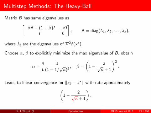
Matrix B has same eigenvalues as[−αΛ + (1 + β)I −βI
I 0
], Λ = diag(λ1, λ2, . . . , λn),
where λi are the eigenvalues of ∇2f (x∗).
Choose α, β to explicitly minimize the max eigenvalue of B, obtain
α =4
L
1
(1 + 1/√κ)2
, β =
(1− 2√
κ+ 1
)2
.
Leads to linear convergence for ‖xk − x∗‖ with rate approximately(1− 2√
κ+ 1
).
S. J. Wright () Optimization MLSS, August 2013 29 / 158

first−order method with momentum
There’s some damping going on! (Like the PID controllers in Schaal’s talkyesterday.)
S. J. Wright () Optimization MLSS, August 2013 30 / 158

Summary: Linear Convergence, Strictly Convex f
Steepest descent: Linear rate approx(
1− 2
κ
);
Heavy-ball: Linear rate approx(
1− 2√κ
).
Big difference! To reduce ‖xk − x∗‖ by a factor ε, need k large enough that(1− 2
κ
)k
≤ ε ⇐ k ≥ κ
2| log ε| (steepest descent)(
1− 2√κ
)k
≤ ε ⇐ k ≥√κ
2| log ε| (heavy-ball)
A factor of√κ difference; e.g. if κ = 1000 (not at all uncommon in
inverse problems), need ∼ 30 times fewer steps.
S. J. Wright () Optimization MLSS, August 2013 31 / 158

Conjugate Gradient
Basic conjugate gradient (CG) step is
xk+1 = xk + αk pk , pk = −∇f (xk ) + γk pk−1.
Can be identified with heavy-ball, with βk =αkγk
αk−1.
However, CG can be implemented in a way that doesn’t require knowledge(or estimation) of L and µ.
Choose αk to (approximately) miminize f along pk ;
Choose γk by a variety of formulae (Fletcher-Reeves, Polak-Ribiere,etc), all of which are equivalent if f is convex quadratic. e.g.
γk =‖∇f (xk )‖2
‖∇f (xk−1)‖2
S. J. Wright () Optimization MLSS, August 2013 32 / 158

Conjugate Gradient
Nonlinear CG: Variants include Fletcher-Reeves, Polak-Ribiere, Hestenes.
Restarting periodically with pk = −∇f (xk ) is useful (e.g. every niterations, or when pk is not a descent direction).
For quadratic f , convergence analysis is based on eigenvalues of A andChebyshev polynomials, min-max arguments. Get
Finite termination in as many iterations as there are distincteigenvalues;
Asymptotic linear convergence with rate approx 1− 2√κ
.
(like heavy-ball.)
(Nocedal and Wright, 2006, Chapter 5)
S. J. Wright () Optimization MLSS, August 2013 33 / 158

Accelerated First-Order Methods
Accelerate the rate to 1/k2 for weakly convex, while retaining the linearrate (related to
√κ) for strongly convex case.
Nesterov (1983) describes a method that requires κ.
Initialize: Choose x0, α0 ∈ (0, 1); set y0 ← x0.
Iterate: xk+1 ← yk − 1L∇f (yk ); (*short-step*)
find αk+1 ∈ (0, 1): α2k+1 = (1− αk+1)α2
k + αk+1
κ ;
set βk =αk (1− αk )
α2k + αk+1
;
set yk+1 ← xk+1 + βk (xk+1 − xk ).
Still works for weakly convex (κ =∞).
S. J. Wright () Optimization MLSS, August 2013 34 / 158

k
xk+1
xk
yk+1
xk+2
yk+2
y
Separates the “gradient descent” and “momentum” step components.
S. J. Wright () Optimization MLSS, August 2013 35 / 158

Convergence Results: Nesterov
If α0 ≥ 1/√κ, have
f (xk )− f (x∗) ≤ c1 min
((1− 1√
κ
)k
,4L
(√
L + c2k)2
),
where constants c1 and c2 depend on x0, α0, L.
Linear convergence “heavy-ball” rate for strongly convex f ;
1/k2 sublinear rate otherwise.
In the special case of α0 = 1/√κ, this scheme yields
αk ≡1√κ, βk ≡ 1− 2√
κ+ 1.
S. J. Wright () Optimization MLSS, August 2013 36 / 158

FISTA
Beck and Teboulle (2009a) propose a similar algorithm, with a fairly shortand elementary analysis (though still not intuitive).
Initialize: Choose x0; set y1 = x0, t1 = 1;
Iterate: xk ← yk − 1L∇f (yk );
tk+1 ← 12
(1 +
√1 + 4t2
k
);
yk+1 ← xk +tk − 1
tk+1(xk − xk−1).
For (weakly) convex f , converges with f (xk )− f (x∗) ∼ 1/k2.
When L is not known, increase an estimate of L until it’s big enough.
Beck and Teboulle (2009a) do the convergence analysis in 2-3 pages:elementary, but technical.
S. J. Wright () Optimization MLSS, August 2013 37 / 158

A Nonmonotone Gradient Method: Barzilai-Borwein
Barzilai and Borwein (1988) (BB) proposed an unusual choice of αk .Allows f to increase (sometimes a lot) on some steps: non-monotone.
xk+1 = xk − αk∇f (xk ), αk := arg minα‖sk − αzk‖2,
wheresk := xk − xk−1, zk := ∇f (xk )−∇f (xk−1).
Explicitly, we have
αk =sT
k zk
zTk zk
.
Note that for f (x) = 12 xT Ax , we have
αk =sT
k Ask
sTk A2sk
∈[
1
L,
1
µ
].
BB can be viewed as a quasi-Newton method, with the Hessianapproximated by α−1
k I .S. J. Wright () Optimization MLSS, August 2013 38 / 158

Comparison: BB vs Greedy Steepest Descent
S. J. Wright () Optimization MLSS, August 2013 39 / 158

There Are Many BB Variants
use αk = sTk sk/sT
k zk in place of αk = sTk zk/zT
k zk ;
alternate between these two formulae;
hold αk constant for a number (2, 3, 5) of successive steps;
take αk to be the steepest descent step from the previous iteration.
Nonmonotonicity appears essential to performance. Some variants getglobal convergence by requiring a sufficient decrease in f over the worst ofthe last M (say 10) iterates.
The original 1988 analysis in BB’s paper is nonstandard and illuminating(just for a 2-variable quadratic).
In fact, most analyses of BB and related methods are nonstandard, andconsider only special cases. The precursor of such analyses is Akaike(1959). More recently, see Ascher, Dai, Fletcher, Hager and others.
S. J. Wright () Optimization MLSS, August 2013 40 / 158

Adding a Constraint: x ∈ Ω
How to change these methods to handle the constraint x ∈ Ω ?
(assuming that Ω is a closed convex set)
Some algorithms and theory stay much the same,
...if we can involve the constraint x ∈ Ω explicity in the subproblems.
Example: Nesterov’s constant step scheme requires just one calculation tobe changed from the unconstrained version.
Initialize: Choose x0, α0 ∈ (0, 1); set y0 ← x0.
Iterate: xk+1 ← arg miny∈Ω12‖y − [yk − 1
L∇f (yk )]‖22;
find αk+1 ∈ (0, 1): α2k+1 = (1− αk+1)α2
k + αk+1
κ ;
set βk = αk (1−αk )α2
k +αk+1;
set yk+1 ← xk+1 + βk (xk+1 − xk ).
Convergence theory is unchanged.
S. J. Wright () Optimization MLSS, August 2013 41 / 158

Extending to Regularized Optimization
How to change these methods to handle optimization with regularization:
minx
f (x) + τψ(x),
where f is convex and smooth, while ψ is convex but usually nonsmooth.
Often, all that is needed is to change the update step to
xk+1 = arg minx
1
2αk‖x − (xk + αk dk )‖2
2 + τψ(x).
where dk could be a scaled gradient descent step, or something morecomplicated (heavy-ball, accelerated gradient), while αk is the step length.
This is the shrinkage/tresholding step; how to solve it with a nonsmoothψ? We’ll come back to this topic after discussing the need forregularization.
S. J. Wright () Optimization MLSS, August 2013 42 / 158

II. Stochastic Gradient Methods
Deal with (weakly or strongly) convex f . We change the rules a bit in thissection:
Allow f nonsmooth.
Can’t get function values f (x) easily.
At any feasible x , have access only to a cheap unbiased estimate ofan element of the subgradient ∂f .
Common settings are:f (x) = EξF (x , ξ),
where ξ is a random vector with distribution P over a set Ξ. Special case:
f (x) =1
m
m∑i=1
fi (x),
where each fi is convex and nonsmooth.(We focus on this finite-sum formulation, but the ideas generalize.)
S. J. Wright () Optimization MLSS, August 2013 43 / 158

Applications
This setting is useful for machine learning formulations. Given dataxi ∈ Rn and labels yi = ±1, i = 1, 2, . . . ,m, find w that minimizes
τψ(w) +1
m
m∑i=1
`(w ; xi , yi ),
where ψ is a regularizer, τ > 0 is a parameter, and ` is a loss. For linearclassifiers/regressors, have the specific form `(w T xi , yi ).
Example: SVM with hinge loss `(w T xi , yi ) = max(1− yi (w T xi ), 0) andψ = ‖ · ‖1 or ψ = ‖ · ‖2
2.
Example: Logistic classification: `(w T xi , yi ) = log(1 + exp(yi wT xi )). In
regularized version may have ψ(w) = ‖w‖1.
S. J. Wright () Optimization MLSS, August 2013 44 / 158

Subgradients
Recall: For each x in domain of f , g is a subgradient of f at x if
f (z) ≥ f (x) + g T (z − x), for all z ∈ dom f .
Right-hand side is a supporting hyperplane.
The set of subgradients is called the subdifferential, denoted by ∂f (x).
When f is differentiable at x , have ∂f (x) = ∇f (x).
We have strong convexity with modulus µ > 0 if
f (z) ≥ f (x)+g T (z−x)+1
2µ‖z−x‖2, for all x , z ∈ dom f with g ∈ ∂f (x).
Generalizes the assumption ∇2f (x) µI made earlier for smoothfunctions.
S. J. Wright () Optimization MLSS, August 2013 45 / 158

Classical Stochastic Gradient
For the finite-sum objective, get a cheap unbiased estimate of the gradient∇f (x) by choosing an index i ∈ 1, 2, . . . ,m uniformly at random, andusing ∇fi (x) to estimate ∇f (x).
Basic SA Scheme: At iteration k, choose ik i.i.d. uniformly at randomfrom 1, 2, . . . ,m, choose some αk > 0, and set
xk+1 = xk − αk∇fik (xk ).
Note that xk+1 depends on all random indices up to iteration k, i.e.i[k] := i1, i2, . . . , ik.When f is strongly convex, the analysis of convergence of expected squareerror E (‖xk − x∗‖2) is fairly elementary — see Nemirovski et al. (2009).
Define ak = 12 E (‖xk − x∗‖2). Assume there is M > 0 such that
1
m
m∑i=1
‖∇fi (x)‖22 ≤ M.
S. J. Wright () Optimization MLSS, August 2013 46 / 158

Rate: 1/k
Thus
1
2‖xk+1 − x∗‖2
2
=1
2‖xk − αk∇fik (xk )− x∗‖2
=1
2‖xk − x∗‖2
2 − αk (xk − x∗)T∇fik (xk ) +1
2α2
k‖∇fik (xk )‖2.
Taking expectations, get
ak+1 ≤ ak − αk E [(xk − x∗)T∇fik (xk )] +1
2α2
k M2.
For middle term, have
E [(xk − x∗)T∇fik (xk )] = Ei[k−1]Eik [(xk − x∗)T∇fik (xk )|i[k−1]]
= Ei[k−1](xk − x∗)T gk ,
S. J. Wright () Optimization MLSS, August 2013 47 / 158

... wheregk := Eik [∇fik (xk )|i[k−1]] ∈ ∂f (xk ).
By strong convexity, have
(xk − x∗)T gk ≥ f (xk )− f (x∗) +1
2µ‖xk − x∗‖2 ≥ µ‖xk − x∗‖2.
Hence by taking expectations, we get E [(xk − x∗)T gk ] ≥ 2µak . Then,substituting above, we obtain
ak+1 ≤ (1− 2µαk )ak +1
2α2
k M2.
When
αk ≡1
kµ,
a neat inductive argument (below) reveals the 1/k rate:
ak ≤Q
2k, for Q := max
(‖x1 − x∗‖2,
M2
µ2
).
S. J. Wright () Optimization MLSS, August 2013 48 / 158

Inductive Proof of 1/k Rate
Clearly true for k = 1. Otherwise:
ak+1 ≤ (1− 2µαk )ak +1
2α2
k M2
≤(
1− 2
k
)ak +
M2
2k2µ2
≤(
1− 2
k
)Q
2k+
Q
2k2
=(k − 1)
2k2Q
=k2 − 1
k2
Q
2(k + 1)
≤ Q
2(k + 1),
as claimed.
S. J. Wright () Optimization MLSS, August 2013 49 / 158
But... What if we don’t know µ? Or if µ = 0?
The choice αk = 1/(kµ) requires strong convexity, with knowledge of themodulus µ. An underestimate of µ can greatly degrade the performance ofthe method (see example in Nemirovski et al. (2009)).
Now describe a Robust Stochastic Approximation approach, which has arate 1/
√k (in function value convergence), and works for weakly convex
nonsmooth functions and is not sensitive to choice of parameters in thestep length.
This is the approach that generalizes to mirror descent, as discussed later.
S. J. Wright () Optimization MLSS, August 2013 50 / 158

Robust SA
At iteration k :
set xk+1 = xk − αk∇fik (xk ) as before;
set
xk =
∑ki=1 αi xi∑k
i=1 αi
.
For any θ > 0, choose step lengths to be
αk =θ
M√
k.
Then f (xk ) converges to f (x∗) in expectation with rate approximately(log k)/k1/2.
(The choice of θ is not critical.)
S. J. Wright () Optimization MLSS, August 2013 51 / 158

Analysis of Robust SA
The analysis is again elementary. As above (using i instead of k), have:
αi E [(xi − x∗)T gi ] ≤ ai − ai+1 +1
2α2
i M2.
By convexity of f , and gi ∈ ∂f (xi ):
f (x∗) ≥ f (xi ) + g Ti (x∗ − xi ),
thus
αi E [f (xi )− f (x∗)] ≤ ai − ai+1 +1
2α2
i M2,
so by summing iterates i = 1, 2, . . . , k , telescoping, and using ak+1 > 0:
k∑i=1
αi E [f (xi )− f (x∗)] ≤ a1 +1
2M2
k∑i=1
α2i .
S. J. Wright () Optimization MLSS, August 2013 52 / 158

Thus dividing by∑
i=1 αi :
E
[∑ki=1 αi f (xi )∑k
i=1 αi
− f (x∗)
]≤
a1 + 12 M2
∑ki=1 α
2i∑k
i=1 αi
.
By convexity, we have
f (xk ) = f
(∑ki=1 αi xi∑k
i=1 αi
)≤∑k
i=1 αi f (xi )∑ki=1 αi
,
so obtain the fundamental bound:
E [f (xk )− f (x∗)] ≤a1 + 1
2 M2∑k
i=1 α2i∑k
i=1 αi
.
S. J. Wright () Optimization MLSS, August 2013 53 / 158
By substituting αi = θM√
i, we obtain
E [f (xk )− f (x∗)] ≤a1 + 1
2θ2∑k
i=11i
θM
∑ki=1
1√i
≤ a1 + θ2 log(k + 1)θM
√k
= M[a1
θ+ θ log(k + 1)
] 1√k.
That’s it!
There are other variants — periodic restarting, averaging just over therecent iterates. These can be analyzed with the basic bound above.
S. J. Wright () Optimization MLSS, August 2013 54 / 158

Constant Step Size
We can also get rates of approximately 1/k for the strongly convex case,without performing iterate averaging. The tricks are to
define the desired threshold ε for ak in advance, and
use a constant step size.
Recall the bound on ak+1 from a few slides back, and set αk ≡ α:
ak+1 ≤ (1− 2µα)ak +1
2α2M2.
Apply this recursively to get
ak ≤ (1− 2µα)k a0 +αM2
4µ.
Given ε > 0, find α and K so that both terms on the right-hand side areless than ε/2. The right values are:
α :=2εµ
M2, K :=
M2
4εµ2log(a0
2ε
).
S. J. Wright () Optimization MLSS, August 2013 55 / 158

Constant Step Size, continued
Clearly the choice of α guarantees that the second term is less than ε/2.
For the first term, we obtain k from an elementary argument:
(1− 2µα)k a0 ≤ ε/2
⇔ k log(1− 2µα) ≤ − log(2a0/ε)
⇐ k(−2µα) ≤ − log(2a0/ε) since log(1 + x) ≤ x
⇔ k ≥ 1
2µαlog(2a0/ε),
from which the result follows, by substituting for α in the right-hand side.
If µ is underestimated by a factor of β, we undervalue α by the samefactor, and K increases by 1/β. (Easy modification of the analysis above.)
Thus, underestimating µ gives a mild performance penalty.
S. J. Wright () Optimization MLSS, August 2013 56 / 158

Constant Step Size: Summary
PRO: Avoid averaging, 1/k sublinear convergence, insensitive tounderestimates of µ.
CON: Need to estimate probably unknown quantities: besides µ, we needM (to get α) and a0 (to get K ).
We use constant size size in the parallel SG approach Hogwild!, to bedescribed later.
But the step is chosen by trying different options and seeing which seemsto be converging fastest. We don’t actually try to estimate all thequantities in the theory and construct α that way.
S. J. Wright () Optimization MLSS, August 2013 57 / 158

Mirror Descent
The step from xk to xk+1 can be viewed as the solution of a subproblem:
xk+1 = arg minz∇fik (xk )T (z − xk ) +
1
2αk‖z − xk‖2
2,
a linear estimate of f plus a prox-term. This provides a route to handlingconstrained problems, regularized problems, alternative prox-functions.
For the constrained problem minx∈Ω f (x), simply add the restriction z ∈ Ωto the subproblem above.
We may use other prox-functions in place of (1/2)‖z − x‖22 above. Such
alternatives may be particularly well suited to particular constraint sets Ω.
Mirror Descent is the term used for such generalizations of the SAapproaches above.
S. J. Wright () Optimization MLSS, August 2013 58 / 158

Mirror Descent cont’d
Given constraint set Ω, choose a norm ‖ · ‖ (not necessarily Euclidean).Define the distance-generating function ω to be a strongly convex functionon Ω with modulus 1 with respect to ‖ · ‖, that is,
(ω′(x)− ω′(z))T (x − z) ≥ ‖x − z‖2, for all x , z ∈ Ω,
where ω′(·) denotes an element of the subdifferential.
Now define the prox-function V (x , z) as follows:
V (x , z) = ω(z)− ω(x)− ω′(x)T (z − x).
This is also known as the Bregman distance. We can use it in thesubproblem in place of 1
2‖ · ‖2:
xk+1 = arg minz∈Ω∇fik (xk )T (z − xk ) +
1
αkV (z , xk ).
S. J. Wright () Optimization MLSS, August 2013 59 / 158

Bregman distance is the deviation of ω from linearity:
ω
x z
V(x,z)
S. J. Wright () Optimization MLSS, August 2013 60 / 158

Bregman Distances: Examples
For any Ω, we can use ω(x) := (1/2)‖x − x‖22, leading to the “universal”
prox-functionV (x , z) = (1/2)‖x − z‖2
2
For the simplex
Ω = x ∈ Rn : x ≥ 0,n∑
i=1
xi = 1,
we can use instead the 1-norm ‖ · ‖1, choose ω to be the entropy function
ω(x) =n∑
i=1
xi log xi ,
leading to Bregman distance (Kullback-Liebler divergence)
V (x , z) =n∑
i=1
zi log(zi/xi )
(standard measure of distance between two probability distributions).S. J. Wright () Optimization MLSS, August 2013 61 / 158

Applications to SVM
SA techniques have an obvious application to linear SVM classification. Infact, they were proposed in this context and analyzed independently byresearchers in the ML community for some years.
Codes: SGD (Bottou, 2012), PEGASOS (Shalev-Shwartz et al., 2007).
Tutorial: Stochastic Optimization for Machine Learning, (Srebro andTewari, 2010) for many more details on the connections betweenstochastic optimization and machine learning.
Related Work: Zinkevich (2003) on online convex programming. Aimingto approximate the minimize the average of a sequence of convexfunctions, presented sequentially. No i.i.d. assumption, regret-basedanalysis. Take steplengths of size O(k−1/2) in gradient ∇fk (xk ) of latestconvex function. Average regret is O(k−1/2).
S. J. Wright () Optimization MLSS, August 2013 62 / 158
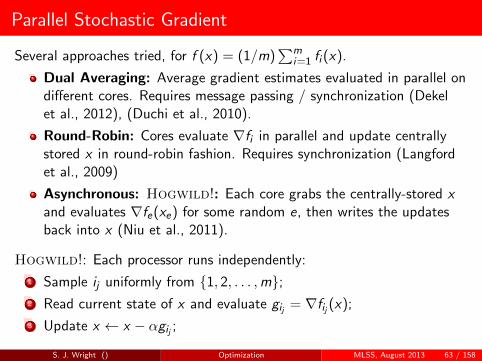
Parallel Stochastic Gradient
Several approaches tried, for f (x) = (1/m)∑m
i=1 fi (x).
Dual Averaging: Average gradient estimates evaluated in parallel ondifferent cores. Requires message passing / synchronization (Dekelet al., 2012), (Duchi et al., 2010).
Round-Robin: Cores evaluate ∇fi in parallel and update centrallystored x in round-robin fashion. Requires synchronization (Langfordet al., 2009)
Asynchronous: Hogwild!: Each core grabs the centrally-stored xand evaluates ∇fe(xe) for some random e, then writes the updatesback into x (Niu et al., 2011).
Hogwild!: Each processor runs independently:
1 Sample ij uniformly from 1, 2, . . . ,m;2 Read current state of x and evaluate gij = ∇fij (x);
3 Update x ← x − αgij ;
S. J. Wright () Optimization MLSS, August 2013 63 / 158

Hogwild! Convergence
Updates can be old by the time they are applied, but we assume abound τ on their age.
Niu et al. (2011) analyze the case in which the update is applied tojust one v ∈ e, but can be extended easily to update the full edge e,provided this is done atomically.
Processors can overwrite each other’s work, but sparsity of ∇fe helps— updates to not interfere too much.
Analysis of Niu et al. (2011) recently simplified / generalized by Richtarik(2012).
In addition to L, µ, M, a0 defined above, also define quantities thatcapture the size and interconnectivity of the subvectors xe .
ρi = |j : fi and fj have overlapping support|;ρ =
∑mi=1 ρi/m2: average rate of overlapping subvectors.
S. J. Wright () Optimization MLSS, August 2013 64 / 158

Hogwild! Convergence
Given ε ∈ (0, a0/L), we have
min0≤j≤k
E (f (xj )− f (x∗)) ≤ ε,
for constant step size
αk ≡µε
(1 + 2τρ)LM2|E |2
and k ≥ K , where
K =(1 + 2τρ)LM2m2
µ2εlog
(2La0
ε− 1
).
Broadly, recovers the sublinear 1/k convergence rate seen in regular SGD,with the delay τ and overlap measure ρ both appearing linearly.
S. J. Wright () Optimization MLSS, August 2013 65 / 158

Hogwild! Performance
Hogwild! compared with averaged gradient (AIG) and round-robin (RR).Experiments run on a 12-core machine. (10 cores used for gradientevaluations, 2 cores for data shuffling.)
S. J. Wright () Optimization MLSS, August 2013 66 / 158

Hogwild! Performance
S. J. Wright () Optimization MLSS, August 2013 67 / 158

III. Higher-Order Methods
Methods whose steps use second-order information about the objective fand constraints. This information can be
Calculated exactly (Newton);
Approximated, by inspecting changes in the gradient over previousiterations (quasi-Newton);
Approximated by finite-differencing on the gradient;
Approximated by re-use from a nearby point;
Approximated by sampling.
Newton’s method is based on a quadratic Taylor-series approximation of asmooth objective f around the current point x :
f (x + d) ≈ q(x ; d) := f (x) +∇f (x)T d +1
2dT∇2f (x)d .
If ∇2f (x) is positive definite (as near the solution x∗), the Newton step isthe d that minimizes q(·; x), explicitly:
d = −∇2f (x)−1∇f (x).
S. J. Wright () Optimization MLSS, August 2013 68 / 158

Can it be practical?
Isn’t it too expensive to compute ∇2f ? Too expensive to store it for largen? What about nonsmooth functions?
For many learning applications, f is often composed of simplefunctions, so writing down second derivatives is often easy. Not thatwe always need them...
∇2f may have sparsity, or other structure that allows it to becomputed and stored efficiently.
In many learning applications, nonsmoothness often enters in a highlystructured way that can be accounted for explicitly, e.g. f (x) + τ‖x‖1.
Often don’t need ∇2f — use approximations instead.
In learning and data analysis, the interesting stuff is often happening on alow-dimensional manifold. We might be able to home in on this manifoldusing first-order methods, then switch to higher-order to improveperformance on the later stages.
S. J. Wright () Optimization MLSS, August 2013 69 / 158

Implementing Newton’s Method
In some cases, it’s practical to compute the Hessian ∇2f (x) explicitly, andsolve for d by factoring and back-substitution:
∇2f (x)d = −∇f (x).
Newton’s method has local quadratic convergence:
‖xk+1 − x∗‖ = O(‖xk − x∗‖2).
When the Hessian is not positive definite, can modify the quadraticapproximation to ensure that it still has a solution, e.g. by adding amultiple of I to the diagonal:
(∇2f (x) + δI )d = −∇f (x), for some δ ≥ 0.
(“Damped Newton” or “Levenberg-Marquardt”)
If we replace ∇2f (x) by 0 and set δ = 1/αk , we recover steepest descent.
Typically do a line search along dk to ensure sufficient decrease in f .S. J. Wright () Optimization MLSS, August 2013 70 / 158

Inexact Newton
We can use an iterative method to solve the Newton equations
∇2f (x)d = −∇f (x),
for example, conjugate gradient. These iterative methods often requirematrix-vector multiplications as the key operations:
v ← ∇2f (x)u.
These can be performed approximately without knowledge of ∇2f (x), byusing finite differencing:
∇2f (x)u ≈ [∇f (x + εu)−∇f (x)]/ε,
for some small scalar ε. Each “inner iteration” of the iterative methodcosts one gradient evaluation.
S. J. Wright () Optimization MLSS, August 2013 71 / 158

Sampled Newton
A cheap estimate of ∇f (x) may be available by sampling.
When f has a partially separable form (common in learning applications):
f (x) =1
m
m∑i=1
fi (x),
(with m huge), we have
∇2f (x) =1
m
m∑i=1
∇2fi (x),
we can thus choose a subset B ⊂ 1, 2, . . . ,m randomly, and define theapproximate Hessian Hk as
Hk =1
|B|∑i∈B∇2fi (xk ),
Has been useful in deep learning / speech applications (Byrd et al., 2011).S. J. Wright () Optimization MLSS, August 2013 72 / 158
Quasi-Newton Methods
Maintains an approximation to the Hessian that’s filled in usinginformation gained on successive steps.
Generate sequence Bk of approximate Hessians alongside the iteratesequence xk, and calculate steps dk by solving
Hk dk = −∇f (xk ).
Update from Bk → Bk+1 so that
Approx Hessian mimics the behavior of the true Hessian over this step:
∇2f (xk+1)sk ≈ yk ,
where sk := xk+1 − xk , yk := ∇f (xk+1)−∇f (xk ), so we enforce
Bk+1sk = yk
Make the smallest change consistent with this property (Occamstrikes again!)
Maintain positive definiteness.S. J. Wright () Optimization MLSS, August 2013 73 / 158
BFGS
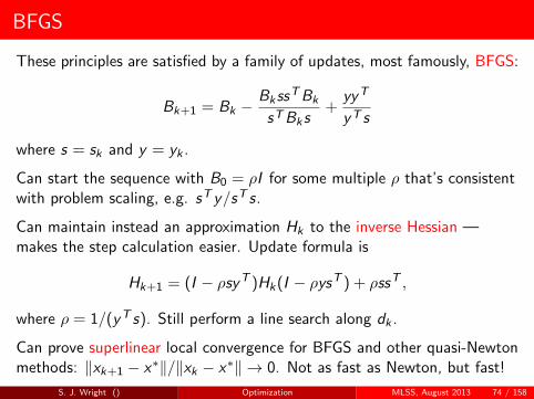
These principles are satisfied by a family of updates, most famously, BFGS:
Bk+1 = Bk −Bk ssT Bk
sT Bk s+
yy T
y T s
where s = sk and y = yk .
Can start the sequence with B0 = ρI for some multiple ρ that’s consistentwith problem scaling, e.g. sT y/sT s.
Can maintain instead an approximation Hk to the inverse Hessian —makes the step calculation easier. Update formula is
Hk+1 = (I − ρsy T )Hk (I − ρysT ) + ρssT ,
where ρ = 1/(y T s). Still perform a line search along dk .
Can prove superlinear local convergence for BFGS and other quasi-Newtonmethods: ‖xk+1 − x∗‖/‖xk − x∗‖ → 0. Not as fast as Newton, but fast!
S. J. Wright () Optimization MLSS, August 2013 74 / 158

LBFGS
LBFGS doesn’t store the n × n matrices Hk or Bk from BFGS explicitlybut rather keeps track of sk and yk from the last few iterations (say,m = 5 or 10), and reconstructs these matrices as needed.
That is, take an initial matrix (B0 or H0) and assume that m steps havebeen taken since. A simple procedure computes Bk u via a series of innerand outer products with the matrices sk−j and yk−j from the last miterations: j = 0, 1, 2, . . . ,m − 1.
Suitable for problems where n is large. Requires 2mn storage and O(mn)linear algebra operations, plus the cost of function and gradientevaluations, and line search.
No superlinear convergence proved, but good behavior is observed on awide range of applications.
(Liu and Nocedal, 1989)
S. J. Wright () Optimization MLSS, August 2013 75 / 158

Newton’s Method for Nonlinear Equations
Given the smooth, square nonlinear equations F (x) = 0 whereF : Rn → Rn (not an optimization problem, but the algorithms arerelated!) we can use a first-order Taylor series expansion:
F (x + d) = F (x) + J(x)d + O(‖d‖2),
where J(x) is the Jacobian (the n × n matrix of first partial derivatives)whose (i , j) element is ∂Fi/∂xj . (Not necessarily symmetric.)
At iteration k , define the Newton step to be dk such that
F (xk ) + J(xk )dk = 0.
If there is a solution x∗ at which F (x∗) = 0 and J(x∗) is nonsingular, thenNewton’s method again has local quadratic convergence. (Kantorovich.)
Useful in interior-point methods — see below.
S. J. Wright () Optimization MLSS, August 2013 76 / 158

Interior-Point Methods
Primal-dual interior-point methods are a powerful class of algorithms forlinear programming and convex quadratic programming — both in theoryand practice.
Also simple elementary to motivate and implement!
minx
1
2xT Qx + cT x s.t. Ax = b, x ≥ 0,
where Q is symmetric positive semidefinite. (LP is a special case.)Optimality conditions are that there exist vectors λ and s such that
Qx + c − ATλ− s = 0, Ax = b, (x , s) ≥ 0, xi si = 0, i = 1, 2, . . . , n.
Defining
X = diag(x1, x2, . . . , xn), S = diag(s1, s2, . . . , sn),
we can write the last condition as XSe = 0, where e = (1, 1, . . . , 1)T .S. J. Wright () Optimization MLSS, August 2013 77 / 158

Thus can write the optimality conditions as a square system ofconstrained, nonlinear equations:Qx + c − ATλ− s
Ax − bXSe
= 0, (x , s) ≥ 0.
Primal-dual interior-point methods generate iterates (xk , λk , sk ) with
(xk , sk ) > 0 (interior).
Each step (∆xk ,∆λk ,∆sk ) is a Newton step on a perturbed versionof the equations. (The perturbation eventually goes to zero.)
Use steplength αk to maintain (xk+1, sk+1) > 0. Set
(xk+1, λk+1, sk+1) = (xk , λk , sk ) + αk (∆xk ,∆λk ,∆sk ).
S. J. Wright () Optimization MLSS, August 2013 78 / 158

Perturbed Newton step is a linear system:Q −AT −IA 0 0S 0 X
∆xk
∆λk
∆sk
=
r kx
r kλ
r kc
where
r kx = −(Qxk + c − ATλk − sk )
r kλ = −(Axk − b)
r kc = −X k Sk e + σkµk e
r kx , r k
λ , r kc are current redisuals, µk = (xk )T sk/n is the current duality gap,
and σk ∈ (0, 1] is a centering parameter.
Typically there is a lot of structure in the system than can be exploited.Do block elimination, for a start.
See Wright (1997) for a description of primal-dual methods, Gertz andWright (2003) for a software framework.
S. J. Wright () Optimization MLSS, August 2013 79 / 158

Interior-Point Methods for Classification
Interior-point methods were tried early for compressed sensing, regularizedleast squares, support vector machines.
SVM with hinge loss formulated as a QP, solved with a primal-dualinterior-point method. Included in the OOQP distribution (Gertz andWright, 2003); see also (Fine and Scheinberg, 2001; Ferris andMunson, 2002).
Compressed sensing and LASSO variable selection formulated asbound-constrained QPs and solved with primal-dual; or second-ordercone programs solved with barrier (Candes and Romberg, 2005)
However they were mostly superseded by first-order methods.
Stochastic gradient in machine learning (low accuracy, simple dataaccess);
Gradient projection (GPSR) and prox-gradient (SpaRSA, FPC) incompressed sensing (require only matrix-vector multiplications).
Is it time to reconsider interior-point methods?S. J. Wright () Optimization MLSS, August 2013 80 / 158

Compressed Sensing: Splitting and Conditioning
Consider the `2-`1 problem
minx
1
2‖Bx − b‖2
2 + τ‖x‖1,
where B ∈ Rm×n. Recall the bound constrained convex QP formulation:
minu≥0,v≥0
1
2‖B(u − v)− b‖2
2 + τ1T (u + v).
B has special properties associated with compressed sensing matrices (e.g.RIP) that make the problem well conditioned.
(Though the objective is only weakly convex, RIP ensures that whenrestricted to the optimal support, the active Hessian submatrix is wellconditioned.)
S. J. Wright () Optimization MLSS, August 2013 81 / 158

Compressed Sensing via Primal-Dual Interior-Point
Fountoulakis et al. (2012) describe an approach that solves thebounded-QP formulation.
Uses a vanilla primal-dual interior-point framework.
Solves the linear system at each interior-point iteration with aconjugate gradient (CG) method.
Preconditions CG with a simple matrix that exploits the RIPproperties of B.
Matrix for each linear system in the interior point solver has the form
M :=
[BT B −BT B−BT B BT B
]+
[U−1S 0
0 V−1T
],
where U = diag(u), V = diag(v), and S = diag(s) and T = diag(t) areconstructed from the Lagrange multipliers for the bound u ≥ 0, v ≥ 0.
S. J. Wright () Optimization MLSS, August 2013 82 / 158

The preconditioner replaces BT B by (m/n)I . Makes sense according tothe RIP properties of B.
P :=m
n
[I −I−I I
]+
[U−1S 0
0 V−1T
],
Convergence of preconditioned CG depends on the eigenvalue distributionof P−1M. Gondzio and Fountoulakis (2013) shows that the gap betweenlargest and smallest eigenvalues actually decreases as the interior-pointiterates approach a solution. (The gap blows up to ∞ for thenon-preconditioned system.)
Overall, the strategy is competitive with first-order methods, on randomtest problems.
S. J. Wright () Optimization MLSS, August 2013 83 / 158

Preconditioning: Effect on Eigenvalue Spread / Solve Time
Red = preconditioned, Blue = non-preconditioned.
S. J. Wright () Optimization MLSS, August 2013 84 / 158
Inference via Optimization
Many inference problems are formulated as optimization problems:
image reconstruction
image restoration/denoising
supervised learning
unsupervised learning
statistical inference
...
Standard formulation:
observed data: y
unknown object (signal, image, vector, matrix,...): x
inference criterion:x ∈ arg min
xg(x , y)
S. J. Wright () Optimization MLSS, August 2013 85 / 158

Inference via Optimization
Inference criterion: x ∈ arg minx
g(x , y)
g comes from the application domain (machine learning, signal processing,inverse problems, statistics, bioinformatics,...); examples ahead.
Typical structure of g : g(x , y) = h(x , y) + τψ(x)
h(x , y) → how well x “fits”/“explains” the data y ;(data term, log-likelihood, loss function, observation model,...)
ψ(x) → knowledge/constraints/structure: the regularizer
τ ≥ 0: the regularization parameter.
Since y is fixed, we often write simply f (x) = h(x , y).
S. J. Wright () Optimization MLSS, August 2013 86 / 158

IV-A. Sparse Optimization: Formulations
Inference criterion, with regularizer ψ: minx
f (x) + τψ(x)
Typically, the unknown is a vector x ∈ Rn or a matrix x ∈ Rn×m.
Common regularizers impose/encourage one (or a combination of) thefollowing characteristics:
small norm (vector or matrix)
sparsity (few nonzeros)
specific nonzero patterns (e.g., group/tree structure)
low-rank (matrix)
smoothness or piece-wise smoothness
S. J. Wright () Optimization MLSS, August 2013 87 / 158

Alternative Formulations for Sparse Optimization
Tikhonov regularization: minx
f (x) + τψ(x)
Morozov regularization:min
xψ(x)
subject to f (x) ≤ ε
Ivanov regularization:min
xf (x)
subject to ψ(x) ≤ δ
Under mild conditions, these are all equivalent.
Morozov and Ivanov can be written as Tikhonov using indicator functions.
Which one to use? Depends on problem and context.
S. J. Wright () Optimization MLSS, August 2013 88 / 158

Cardinality (`0) is hard to deal with!
Finding the sparsest solution is NP-hard (Muthukrishnan, 2005).
w = arg minw‖w‖0 s.t. ‖Aw − y‖2
2 ≤ δ.
The related best subset selection problem is also NP-hard (Amaldi andKann, 1998; Davis et al., 1997).
w = arg minw‖Aw − y‖2
2 s.t. ‖w‖0 ≤ τ.
Under conditions, we can use `1 as a proxy for `0! This is the central issuein compressive sensing (CS) (Candes et al., 2006a; Donoho, 2006)
S. J. Wright () Optimization MLSS, August 2013 89 / 158

Compressed Sensing — Reconstructions with `1
S. J. Wright () Optimization MLSS, August 2013 90 / 158

Compressive Sensing in a Nutshell
Even in the noiseless case, it seems impossible to recover w from y
...unless, w is sparse and A has some properties.
If w is sparse enough and A has certain properties, then w is stablyrecovered via (Haupt and Nowak, 2006)
w = arg minw‖w‖0
s. t. ‖Aw − y‖ ≤ δ NP-hard!
S. J. Wright () Optimization MLSS, August 2013 91 / 158

Compressive Sensing in a Nutshell
Even in the noiseless case, it seems impossible to recover w from y...unless, w is sparse and A has some properties.
If w is sparse enough and A has certain properties, then w is stablyrecovered via (Haupt and Nowak, 2006)
w = arg minw‖w‖0
s. t. ‖Aw − y‖ ≤ δ NP-hard!
S. J. Wright () Optimization MLSS, August 2013 91 / 158

Compressive Sensing in a Nutshell
The key assumption on A is defined variously as incoherence or restrictedisometry (RIP). When such a property holds, we can replace `0 with `1 inthe formulation: (Candes et al., 2006b):
w = arg minw‖w‖1
subject to ‖Aw − y‖ ≤ δ convex problem
Matrix A satisfies the RIP of order k, with constant δk ∈ (0, 1), if
‖w‖0 ≤ k ⇒ (1− δk)‖w‖22 ≤ ‖Aw‖ ≤ (1 + δk)‖w‖2
2
...i.e., for k-sparse vectors, A is approximately an isometry. Alternatively,say that “all k-column submatrices of A are nearly orthonormal.”
Other properties (spark and null space property (NSP)) can be used.
Caveat: checking RIP, NSP, spark is NP-hard (Tillmann and Pfetsch,2012), but these properties are usually satisfied by random matrices.
S. J. Wright () Optimization MLSS, August 2013 92 / 158

Compressive Sensing in a Nutshell
The key assumption on A is defined variously as incoherence or restrictedisometry (RIP). When such a property holds, we can replace `0 with `1 inthe formulation: (Candes et al., 2006b):
w = arg minw‖w‖1
subject to ‖Aw − y‖ ≤ δ convex problem
Matrix A satisfies the RIP of order k, with constant δk ∈ (0, 1), if
‖w‖0 ≤ k ⇒ (1− δk )‖w‖22 ≤ ‖Aw‖ ≤ (1 + δk )‖w‖2
2
...i.e., for k-sparse vectors, A is approximately an isometry. Alternatively,say that “all k-column submatrices of A are nearly orthonormal.”
Other properties (spark and null space property (NSP)) can be used.
Caveat: checking RIP, NSP, spark is NP-hard (Tillmann and Pfetsch,2012), but these properties are usually satisfied by random matrices.
S. J. Wright () Optimization MLSS, August 2013 92 / 158

Underconstrained Systems
Let x be the sparsest solution of Ax = y , where A ∈ Rm×n and m < n.
x = arg min ‖x‖0 s.t. Ax = y .
Consider instead the convex, `1 norm version:
minx‖x‖1 s.t. Ax = y .
Of course, x solves this problem too, if ‖x + v‖1 ≥ ‖x‖1, ∀v ∈ ker(A).
Recall: ker(A) = x ∈ Rn : Ax = 0 is the kernel (a.k.a. null space) of A.
Coming Up: elementary analysis by Yin and Zhang (2008), based on workby Kashin (1977) and Garnaev and Gluskin (1984).
S. J. Wright () Optimization MLSS, August 2013 93 / 158

Equivalence Between `1 and `0 Optimization
Minimum `0 (sparsest) solution: x ∈ arg min ‖x‖0 s.t. Ax = y .
x is also a solution of min ‖x‖1 s.t. Ax = y , provided that
‖x + v‖1 ≥ ‖x‖1, ∀v ∈ ker(A).
Letting S = i : xi 6= 0 and Z = 1, ..., n \ S , we have
‖x + v‖1 = ‖xS + vS‖1 + ‖vZ‖1
≥ ‖xS‖1 + ‖vZ‖1 − ‖vS‖1
= ‖x‖1 + ‖v‖1 − 2‖vS‖1
≥ ‖x‖1 + ‖v‖1 − 2√
k‖v‖2.
Hence, x minimizes the convex formuation if 12‖v‖1
‖v‖2≥√
k , ∀v ∈ ker(A)
...but, in general, we have only: 1 ≤ ‖v‖1
‖v‖2≤√
n.
However, we may have ‖v‖1
‖v‖2 1, if v is restricted to a random subspace.
S. J. Wright () Optimization MLSS, August 2013 94 / 158

Bounding the `1/`2 Ratio in Random Matrices
If the elements of A ∈ Rm×n are sampled i.i.d. from N (0, 1) (zero mean,unit variance Gaussian), then, with high probability,
‖v‖1
‖v‖2≥ C
√m√
log(n/m), for all v ∈ ker(A),
for some constant C (based on concentration of measure phenomena).
Thus, with high probability, x ∈ G , if
m ≥ 4
C 2k log n.
Conclusion: Can solve under-determined system, where A has i.i.d.N (0, 1) elements, by solving the convex problem
minx‖x‖1 s.t. Ax = b,
if the solution is sparse enough, and A is random with O(k log n) rows.S. J. Wright () Optimization MLSS, August 2013 95 / 158

Ratio ‖v‖1/‖v‖2 on Random Null Spaces
Random A ∈ R4×7, showing ratio ‖v‖1 for v ∈ ker(A) with ‖v‖2 = 1
Blue: ‖v‖1 ≈ 1. Red: ratio ≈√
7. Note that ‖v‖1 is well away from thelower bound of 1 over the whole nullspace.
S. J. Wright () Optimization MLSS, August 2013 96 / 158

Ratio ‖v‖1/‖v‖2 on Random Null Spaces
The effect grows more pronounced as m/n grows.Random A ∈ R17×20, showing ratio ‖v‖1 for v ∈ N(A) with ‖v‖2 = 1.
Blue: ‖v‖1 ≈ 1. Red: ‖v‖1 ≈√
20. Note that ‖v‖1 is closer to upperbound throughout.
S. J. Wright () Optimization MLSS, August 2013 97 / 158

The Ubiquitous `1 Norm
Lasso (least absolute shrinkage and selection operator) (Tibshirani, 1996)a.k.a. basis pursuit denoising (Chen et al., 1995):
minx
1
2‖Ax − y‖2
2 + τ‖x‖1 or minx‖Ax − y‖2
2 s.t. ‖x‖1 ≤ δ
or, more generally,
minx
f (x) + τ‖x‖1 or minx
f (x) s.t. ‖x‖1 ≤ δ
Widely used outside and much earlier than compressive sensing(statistics, signal processing, neural networks, ...).
Many extensions: namely to express structured sparsity (more later).
Why does `1 yield sparse solutions? (next slides)
How to solve these problems? (this tutorial)
S. J. Wright () Optimization MLSS, August 2013 98 / 158

Why `1 Yields Sparse Solution
w∗ = arg minw ‖Aw − y‖22
s.t. ‖w‖2 ≤ δvs w∗ = arg minw ‖Aw − y‖2
2
s.t. ‖w‖1 ≤ δ
S. J. Wright () Optimization MLSS, August 2013 99 / 158

“Shrinking” with `1
The simplest problem with `1 regularization
w = arg minw
1
2(w − y)2 + τ |w | = soft(y , τ) =
y − τ ⇐ y > τ0 ⇐ |y | ≤ τy + τ ⇐ y < −τ
Contrast with the squared `2 (ridge) regularizer (linear scaling):
w = arg minw
1
2(w − y)2 +
τ
2w 2 =
1
1 + τy .
(No sparsification.)
S. J. Wright () Optimization MLSS, August 2013 100 / 158

“Shrinking” with `1
The simplest problem with `1 regularization
w = arg minw
1
2(w − y)2 + τ |w | = soft(y , τ) =
y − τ ⇐ y > τ0 ⇐ |y | ≤ τy + τ ⇐ y < −τ
Contrast with the squared `2 (ridge) regularizer (linear scaling):
w = arg minw
1
2(w − y)2 +
τ
2w 2 =
1
1 + τy .
(No sparsification.)S. J. Wright () Optimization MLSS, August 2013 100 / 158

Machine/Statistical Learning: Linear Classification
Data N pairs (x1, y1), ..., (xN , yN), where xi ∈ Rd (feature vectors)and yi ∈ −1,+1 (labels).
Goal: find “good” linear classifier (i.e., find the optimal weights):
y = sign([xT 1]w) = sign(
wd+1 +d∑
j=1
wj xj
)
Assumption: data generated i.i.d. by some underlying distribution PX ,Y
Expected error: minw∈Rd+1
E(1Y ([X T 1]w)<0
)impossible! PX ,Y unknown
Empirical error (EE): minw
1N
N∑i=1
h(
yi ([xT 1]w)︸ ︷︷ ︸margin
), where h(z) = 1z<0.
Convexification: EE neither convex nor differentiable (NP-hard problem).Solution: replace h : R→ 0, 1 with convex loss L : R→ R+.
S. J. Wright () Optimization MLSS, August 2013 101 / 158

Machine/Statistical Learning: Linear Classification
Data N pairs (x1, y1), ..., (xN , yN), where xi ∈ Rd (feature vectors)and yi ∈ −1,+1 (labels).
Goal: find “good” linear classifier (i.e., find the optimal weights):
y = sign([xT 1]w) = sign(
wd+1 +d∑
j=1
wj xj
)Assumption: data generated i.i.d. by some underlying distribution PX ,Y
Expected error: minw∈Rd+1
E(1Y ([X T 1]w)<0
)impossible! PX ,Y unknown
Empirical error (EE): minw
1N
N∑i=1
h(
yi ([xT 1]w)︸ ︷︷ ︸margin
), where h(z) = 1z<0.
Convexification: EE neither convex nor differentiable (NP-hard problem).Solution: replace h : R→ 0, 1 with convex loss L : R→ R+.
S. J. Wright () Optimization MLSS, August 2013 101 / 158

Machine/Statistical Learning: Linear Classification
Criterion: minw
N∑i=1
L(
yi (w T xi + b)︸ ︷︷ ︸margin
)︸ ︷︷ ︸
f (w)
+τψ(w)
Regularizer: ψ = `1 ⇒ encourage sparseness ⇒ feature selection
Convex losses: L : R→ R+ is a (preferably convex) loss function.
Misclassification loss: L(z) = 1z<0
Hinge loss: L(z) = max1− z , 0
Logistic loss: L(z) =log(
1+exp(−z))
log 2
Squared loss: L(z) = (z − 1)2
S. J. Wright () Optimization MLSS, August 2013 102 / 158

Machine/Statistical Learning: General Formulation
This formulation cover a wide range of linear ML methods:
minw
N∑i=1
L(yi ([xT 1]w)
)︸ ︷︷ ︸
f (w)
+ τψ(w)
Least squares regression: L(z) = (z − 1)2, ψ(w) = 0.
Ridge regression: L(z) = (z − 1)2, ψ(w) = ‖w‖22.
Lasso regression: L(z) = (z − 1)2, ψ(w) = ‖w‖1
Logistic classification: L(z) = log(1 + exp(−z)) (ridge, ifψ(w) = ‖w‖2
2
Sparse logistic regression: L(z) = log(1 + exp(−z)), ψ(w) = ‖w‖1
Support vector machines: L(z) = max1− z , 0, ψ(w) = ‖w‖22
Boosting: L(z) = exp(−z),
...
S. J. Wright () Optimization MLSS, August 2013 103 / 158

Machine/Statistical Learning: Nonlinear Problems
What about non-linear functions?
Simply use y = φ(x ,w) =D∑
j=1
wj φj (x), where φj : Rd → R
Essentially, nothing changes; computationally, a lot may change!
minw
N∑i=1
L(yi φ(x ,w)
)︸ ︷︷ ︸
f (w)
+ τψ(w)
Key feature: φ(x ,w) is still linear with respect to w , thus f inherits theconvexity of L.
Examples: polynomials, radial basis functions, wavelets, splines, kernels,...
S. J. Wright () Optimization MLSS, August 2013 104 / 158

Structured Sparsity — Groups
Main goal: to promote structural patterns, not just penalize cardinality
Group sparsity: discard/keep entire groups of features (Bach et al., 2012)
density inside each group
sparsity with respect to the groups which are selected
choice of groups: prior knowledge about the intended sparsity patterns
Yields statistical gains if the assumption is correct (Stojnic et al., 2009)
Many applications:
feature template selection (Martins et al., 2011)
multi-task learning (Caruana, 1997; Obozinski et al., 2010)
learning the structure of graphical models (Schmidt and Murphy,2010)
S. J. Wright () Optimization MLSS, August 2013 105 / 158

Example: Sparsity with Multiple Classes
In multi-class (more than just 2 classes) classification, a commonformulation is
y = arg maxy∈1,...,K
xT wy
Weight vector w = (w1, ...,wK ) ∈ RKd has a natural group/gridorganization:
input features
labels
Simple sparsity is wasteful: may still need to keep all the features
Structured sparsity: discard some input features (feature selection)
S. J. Wright () Optimization MLSS, August 2013 106 / 158

Example: Multi-Task Learning
Same thing, except now rows are tasks and columns are features
Example: simultaneous regression (seek function into Rd → Rb)
shared features
task
s
Goal: discard features that are irrelevant for all tasks
Approach: one group per feature (Caruana, 1997; Obozinski et al., 2010)
S. J. Wright () Optimization MLSS, August 2013 107 / 158
Mixed Norm Regularizer
ψ(x) =M∑
i=1
‖x[i ]‖2
where x[i ] is a subvector of x (Zhao et al., 2009).
Sum of infinity norms also used (Turlach et al., 2005).
Three scenarios for groups, progressively harder to deal with:
Non-overlapping Groups
Tree-structured Groups
Graph-structured Groups
S. J. Wright () Optimization MLSS, August 2013 108 / 158

Matrix Inference Problems
Sparsest solution:
From Bx = b ∈ Rp, findx ∈ Rn (p < n).
minx ‖x‖0 s.t. Bx = b
Yields exact solution, undersome conditions.
Lowest rank solution:
From B(X ) = b ∈ Rp, findX ∈ Rm×n (p < m n).
minX rank(X ) s.t. B(X ) = b
Yields exact solution, under someconditions.
Both NP−hard (in general); the same is true of noisy versions:
minX∈Rm×n
rank(X ) s.t. ‖B(X )− b‖22
Under some conditions, the same solution is obtained by replacing rank(X )by the nuclear norm ‖X‖∗ (as any norm, it is convex) (Recht et al., 2010)
S. J. Wright () Optimization MLSS, August 2013 109 / 158

Nuclear Norm Regularization
Tikhonov formulation: minX‖B(X )− b‖2
2︸ ︷︷ ︸f (X )
+ τ‖X‖∗︸ ︷︷ ︸τψ(X )
Linear observations: B : Rm×n → Rp,(B(X )
)i
= 〈B(i),X 〉,
B(i) ∈ Rm×n, and 〈B,X 〉 =∑
ij
Bij Xij = trace(BT X )
Particular case: matrix completion, each matrix B(i) has one 1 and is zeroeverywhere else.
Why does the nuclear norm favor low rank solutions? Let Y = UΛV T bethe singular value decomposition, where Λ = diag
(σ1, ..., σminm,n
); then
arg minX
1
2‖Y − X‖2
F + τ‖X‖∗ = U soft(Λ, τ)︸ ︷︷ ︸may yield zeros
V T
...singular value thresholding (Ma et al., 2011; Cai et al., 2010b)
S. J. Wright () Optimization MLSS, August 2013 110 / 158

Nuclear Norm Regularization
Tikhonov formulation: minX‖B(X )− b‖2
2︸ ︷︷ ︸f (X )
+ τ‖X‖∗︸ ︷︷ ︸τψ(X )
Linear observations: B : Rm×n → Rp,(B(X )
)i
= 〈B(i),X 〉,
B(i) ∈ Rm×n, and 〈B,X 〉 =∑
ij
Bij Xij = trace(BT X )
Particular case: matrix completion, each matrix B(i) has one 1 and is zeroeverywhere else.
Why does the nuclear norm favor low rank solutions?
Let Y = UΛV T bethe singular value decomposition, where Λ = diag
(σ1, ..., σminm,n
); then
arg minX
1
2‖Y − X‖2
F + τ‖X‖∗ = U soft(Λ, τ)︸ ︷︷ ︸may yield zeros
V T
...singular value thresholding (Ma et al., 2011; Cai et al., 2010b)
S. J. Wright () Optimization MLSS, August 2013 110 / 158

Nuclear Norm Regularization
Tikhonov formulation: minX‖B(X )− b‖2
2︸ ︷︷ ︸f (X )
+ τ‖X‖∗︸ ︷︷ ︸τψ(X )
Linear observations: B : Rm×n → Rp,(B(X )
)i
= 〈B(i),X 〉,
B(i) ∈ Rm×n, and 〈B,X 〉 =∑
ij
Bij Xij = trace(BT X )
Particular case: matrix completion, each matrix B(i) has one 1 and is zeroeverywhere else.
Why does the nuclear norm favor low rank solutions? Let Y = UΛV T bethe singular value decomposition, where Λ = diag
(σ1, ..., σminm,n
); then
arg minX
1
2‖Y − X‖2
F + τ‖X‖∗ = U soft(Λ, τ)︸ ︷︷ ︸may yield zeros
V T
...singular value thresholding (Ma et al., 2011; Cai et al., 2010b)S. J. Wright () Optimization MLSS, August 2013 110 / 158

Another Matrix Inference Problem: Inverse Covariance
Consider n samples y1, ..., yn ∈ Rd of a Gaussian r.v. Y ∼ N (µ,C ); thelog-likelihood is
L(P) = log p(y1, ..., yn|P) = log det(P)− trace(SP) + constant
where S = 1n
∑ni=1(yi − µ)(yi − µ)T and P = C−1 (inverse covariance).
Zeros in P reveal conditional independencies between components of Y :
Pij = 0 ⇔ Yi ⊥⊥ Yj |Yk , k 6= i , j
...exploited to infer (in)dependencies among Gaussian variables. Widelyused in computational biology and neuroscience, social network analysis, ...
Sparsity (presence of zeros) in P is encouraged by solving
minP0− log det(P) + trace(SP)︸ ︷︷ ︸
f (P)
+τ ‖vect(P)‖1︸ ︷︷ ︸ψ(P)
where vect(P) = [P1,1, ...,Pd ,d ]T .
S. J. Wright () Optimization MLSS, August 2013 111 / 158

Another Matrix Inference Problem: Inverse Covariance
Consider n samples y1, ..., yn ∈ Rd of a Gaussian r.v. Y ∼ N (µ,C ); thelog-likelihood is
L(P) = log p(y1, ..., yn|P) = log det(P)− trace(SP) + constant
where S = 1n
∑ni=1(yi − µ)(yi − µ)T and P = C−1 (inverse covariance).
Zeros in P reveal conditional independencies between components of Y :
Pij = 0 ⇔ Yi ⊥⊥ Yj |Yk , k 6= i , j
...exploited to infer (in)dependencies among Gaussian variables. Widelyused in computational biology and neuroscience, social network analysis, ...
Sparsity (presence of zeros) in P is encouraged by solving
minP0− log det(P) + trace(SP)︸ ︷︷ ︸
f (P)
+τ ‖vect(P)‖1︸ ︷︷ ︸ψ(P)
where vect(P) = [P1,1, ...,Pd ,d ]T .S. J. Wright () Optimization MLSS, August 2013 111 / 158

Atomic-Norm Regularization
The atomic norm
‖x‖A = inf
t > 0 : x ∈ t conv(A)
= inf∑
a∈Aca : x =
∑a∈A
caa, ca ≥ 0
...assuming that the centroid of A is at the origin.
Example: the `1 norm as an atomic norm
A =
[01
],
[10
],
[0−1
],
[−10
]conv(A) = B1(1) (`1 unit ball).
‖x‖A = inf
t > 0 : x ∈ t B1(1)
= ‖x‖1
S. J. Wright () Optimization MLSS, August 2013 112 / 158

Atomic Norms: More Examples
S. J. Wright () Optimization MLSS, August 2013 113 / 158

Atomic-Norm Regularization
Given an atomic set A, we can adopt an Ivanov formulation
min f (x) s.t. ‖x‖A ≤ δ
(for some δ > 0) tends to recover x with sparse atomic representation.
Can formulate algorithms for the various special cases — but is a generalapproach available for this formulation?
Yes! The conditional gradient! (more later.)
It is also possible to tackle the Tikhonov and Morozov formulations
minx
f (x) + τ‖x‖A and minx‖x‖A s.t. f (x) ≤ ε
(more later).
S. J. Wright () Optimization MLSS, August 2013 114 / 158

Summary: Sparse Optimization Formulations
Many inference, learning, signal/image processing problems can beformulated as optimization problems.
Sparsity-inducing regularizers play an important role in these problems
There are several way to induce sparsity
It is possible to formulate structured sparsity
It is possible to extend the sparsity rationale to other objects, namelymatrices
Atomic norms provide a unified framework for sparsity/simplicityregularization
Now discuss Algorithms for Sparse / Regularized Optimization (SectionIV-B).
S. J. Wright () Optimization MLSS, August 2013 115 / 158

More Basics: Subgradients of Convex Functions
Convexity ⇒ continuity (on the domain of the function).
Convexity 6⇒ differentiability. (Example: ‖x‖1 is convex but notdifferentiable when any components of x are zero).
Subgradients generalize gradients for general convex functions:
v is a subgradient of f at x if f (x ′) ≥ f (x) + v T (x ′ − x)
Subdifferential: ∂f (x) = all subgradients of f at xIf f is differentiable, ∂f (x) = ∇f (x)
linear lower bound nondifferentiable case
S. J. Wright () Optimization MLSS, August 2013 116 / 158

More on Subgradients and Subdifferentials
The subdifferential is a set-valued function:
f : Rd → R ⇒ ∂f : Rd → 2Rd
(power set of Rd )
Example:
f (x) =
−2x − 1, x ≤ −1−x , −1 < x ≤ 0
x2/2, x > 0
∂f (x) =
−2, x < −1
[−2, −1], x = −1−1, −1 < x < 0
[−1, 0], x = 0x, x > 0
x ∈ arg minx f (x) ⇔ 0 ∈ ∂f (x)
S. J. Wright () Optimization MLSS, August 2013 117 / 158

A Key Tool: Moreau’s Proximity Operators: “Shrinks”
Moreau (1962) proximity operator
x ∈ arg minx
1
2‖x − y‖2
2 + ψ(x) =: proxψ(y)
...well defined for convex ψ, since ‖ · −y‖22 is coercive and strictly convex.
Example: (seen above) proxτ |·|(y) = soft(y , τ) = sign(y) max|y | − τ, 0
Block separability: x = (x[1], ..., x[M]) (a partition of the components of x)
ψ(x) =M∑
i=1
ψi (x[i ]) ⇒ (proxψ(y))i = proxψi(y[i ])
Relationship with subdifferential: z = proxψ(y) ⇔ y − z ∈ ∂ψ(z)
S. J. Wright () Optimization MLSS, August 2013 118 / 158
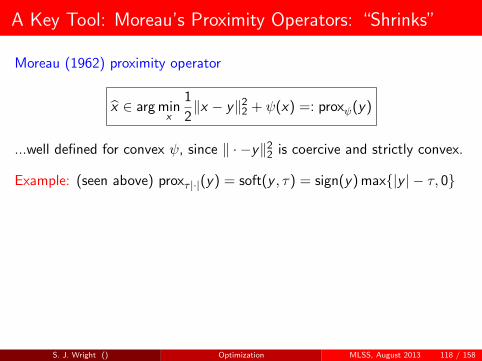

Important Proximity Operators
Soft-thresholding is the proximity operator of the `1 norm.
Consider the indicator ιS of a convex set S;
proxιS (u) = arg minx
1
2‖x − u‖2
2 + ιS(x) = arg minx∈S
1
2‖x − y‖2
2 = PS(u)
...the Euclidean projection on S.
Squared Euclidean norm (separable, smooth):
prox(τ/2)‖·‖22(y) = arg min
x
1
2‖x − y‖2
2 +τ
2‖x‖2
2 =y
1 + τ
Euclidean norm (not separable, nonsmooth):
proxτ‖·‖2(y) =
x‖x‖2
(‖x‖2 − τ), if ‖x‖2 > τ
0 if ‖x‖2 ≤ τ
S. J. Wright () Optimization MLSS, August 2013 119 / 158
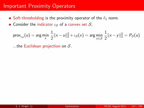

More Proximity Operators
(Combettes and Pesquet, 2011)
S. J. Wright () Optimization MLSS, August 2013 120 / 158

Matrix Nuclear Norm and its Prox Operator
Recall the trace/nuclear norm: ‖X‖∗ =
minm,n∑i=1
σi .
The dual of a Schatten p-norm is a Schatten q-norm, with1q + 1
p = 1. Thus, the dual of the nuclear norm is the spectral norm:
‖X‖∞ = maxσ1, ..., σminm,n
.
If Y = UΛV T is the SVD of Y , we have
proxτ‖·‖∗(Y ) = UΛV T − PX :maxσ1,...,σminm,n≤τ(UΛV T )
= U soft(Λ, τ
)V T .
S. J. Wright () Optimization MLSS, August 2013 121 / 158

Basic Proximal-Gradient Algorithm
Take this step at iteration k :
xk+1 = proxαkψ
(xk − αk∇f (xk )
).
This approach goes by many names, such as
“proximal gradient algorithm” (PGA),
“iterative shrinkage/thresholding” (IST),
“forward-backward splitting” (FBS)
It it has been reinvented several times in different communities:optimization, partial differential equations, convex analysis, signalprocessing, machine learning.
S. J. Wright () Optimization MLSS, August 2013 122 / 158

Convergence of the Proximal-Gradient Algorithm
Basic algorithm: xk+1 = proxαkψ
(xk − αk∇f (xk )
)Generalized (possibly inexact) version:
xk+1 = (1− λk )xk + λk
(proxαkψ
(xk − αk∇f (xk ) + bk
)+ ak
)where ak and bk are “errors” in computing the prox and the gradient;λk is an over-relaxation parameter.
Convergence is guaranteed (Combettes and Wajs, 2006) if
X 0 < inf αk ≤ supαk <2L
X λk ∈ (0, 1], with inf λk > 0
X∑∞
k ‖ak‖ <∞ and∑∞
k ‖bk‖ <∞
S. J. Wright () Optimization MLSS, August 2013 123 / 158

More on IST/FBS/PGA for the `2-`1 Case
Problem: x ∈ G = arg minx∈Rn
12‖B x − b‖2
2 + τ‖x‖1 (recall BT B LI )
IST/FBS/PGA becomes xk+1 = soft(xk − αBT (B x − b), ατ
)with α < 2/L.
The zero set: Z ⊆ 1, ..., n : x ∈ G ⇒ xZ = 0
Zeros are found in a finite number of iterations (Hale et al., 2008):after a finite number of iterations (xk)Z = 0.
After discovery of the zero set, reduces to minimizing anunconstrained quadratic over the nonzero elements of x :N := 1, 2, . . . , n \ Z. By RIP property, the submatrix BT
NBN is wellconditioned, so convergence is typically fast linear.
S. J. Wright () Optimization MLSS, August 2013 124 / 158
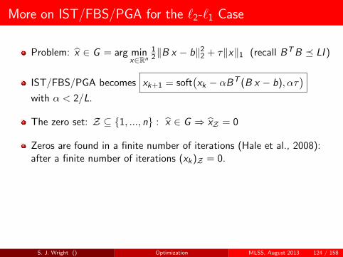
More on IST/FBS/PGA for the `2-`1 Case
Problem: x ∈ G = arg minx∈Rn
12‖B x − b‖2
2 + τ‖x‖1 (recall BT B LI )
IST/FBS/PGA becomes xk+1 = soft(xk − αBT (B x − b), ατ
)with α < 2/L.
The zero set: Z ⊆ 1, ..., n : x ∈ G ⇒ xZ = 0
Zeros are found in a finite number of iterations (Hale et al., 2008):after a finite number of iterations (xk )Z = 0.
After discovery of the zero set, reduces to minimizing anunconstrained quadratic over the nonzero elements of x :N := 1, 2, . . . , n \ Z. By RIP property, the submatrix BT
NBN is wellconditioned, so convergence is typically fast linear.
S. J. Wright () Optimization MLSS, August 2013 124 / 158

Heavy Ball Acceleration: FISTA
FISTA (fast iterative shrinkage-thresholding algorithm) isheavy-ball-type acceleration of IST (based on Nesterov (1983)) (Beckand Teboulle, 2009a).
Initialize: Choose α ≤ 1/L, x0; set y1 = x0, t1 = 1;
Iterate: xk ← proxταψ(yk − α∇f (yk )
);
tk+1 ← 12
(1 +
√1 + 4t2
k
);
yk+1 ← xk +tk − 1
tk+1(xk − xk−1).
Acceleration:
FISTA: f (xk )− f (x) ∼ O
(1
k2
)IST: f (xk)− f (x) ∼ O
(1
k
).
When L is not known, increase an estimate of L until it’s big enough.
S. J. Wright () Optimization MLSS, August 2013 125 / 158

Heavy Ball Acceleration: FISTA
FISTA (fast iterative shrinkage-thresholding algorithm) isheavy-ball-type acceleration of IST (based on Nesterov (1983)) (Beckand Teboulle, 2009a).
Initialize: Choose α ≤ 1/L, x0; set y1 = x0, t1 = 1;
Iterate: xk ← proxταψ(yk − α∇f (yk )
);
tk+1 ← 12
(1 +
√1 + 4t2
k
);
yk+1 ← xk +tk − 1
tk+1(xk − xk−1).
Acceleration:
FISTA: f (xk )− f (x) ∼ O
(1
k2
)IST: f (xk )− f (x) ∼ O
(1
k
).
When L is not known, increase an estimate of L until it’s big enough.
S. J. Wright () Optimization MLSS, August 2013 125 / 158

Acceleration via Larger Steps: SpaRSA
The standard step-size αk ≤ 2L in IST too timid.
The SpARSA (sparse reconstruction by separable approximation)framework proposes bolder choices of αk (Wright et al., 2009a):
Barzilai-Borwein (see above), to mimic Newton steps — or at leastget the scaling right.
keep increasing αk until monotonicity is violated: backtrack.
Convergence to critical points (minima in the convex case) is guaranteedfor a safeguarded version: ensure sufficient decrease w.r.t. the worst valuein previous M iterations.
S. J. Wright () Optimization MLSS, August 2013 126 / 158

Acceleration by Continuation
IST/FBS/PGA can be very slow if τ is very small and/or f is poorlyconditioned.
A very simple acceleration strategy: continuation/homotopy
Initialization: Set τ0 τ , starting point x , factor σ ∈ (0, 1), and k = 0.
Iterations: Find approx solution x(τk ) of minx f (x) + τkψ(x), starting from x ;
if τk = τf STOP;
Set τk+1 ← max(τf , στk ) and x ← x(τk );
Often the solution path x(τ), for a range of values of τ is desired,anyway (e.g., within an outer method to choose an optimal τ)
Shown to be very effective in practice (Hale et al., 2008; Wrightet al., 2009a). Recently analyzed by Xiao and Zhang (2012).
S. J. Wright () Optimization MLSS, August 2013 127 / 158

A Final Touch: Debiasing
Consider problems of the form x ∈ arg minx∈Rn
12‖B x − b‖2
2 + τ‖x‖1
Often, the original goal was to minimize the quadratic term, after thesupport of x had been found. But the `1 term can cause the nonzerovalues of xi to be “suppressed.”
Debiasing:
X find the zero set (complement of the support of x):Z(x) = 1, ..., n \ supp(x).
X solve minx ‖B x − b‖22 s.t. xZ(x) = 0. (Fix the zeros and solve an
unconstrained problem over the support.)
Often, this problem has to be solved using an algorithm that onlyinvolves products by B and BT , since this matrix cannot bepartitioned.
S. J. Wright () Optimization MLSS, August 2013 128 / 158

Identifying Optimal Manifolds
Identification of the manifold of the regularizer ψ on which x∗ lies canimprove algorithm performance, by focusing attention on a reduced space.We can thus evaluate partial gradients and Hessians, restricted to just thisspace.
For nonsmooth regularizer ψ, the optimal manifold is a smooth surfacepassing through x∗ along which the restriction of ψ is smooth.
Example: for ψ(x) = ‖x‖1, have manifold consisting of z with
zi
≥ 0 if x∗i > 0
≤ 0 if x∗i < 0
= 0 if x∗i = 0.
If we know the optimal nonzero components, we know the manifold. Wecould restrict the search to just this set of nonzeros.
S. J. Wright () Optimization MLSS, August 2013 129 / 158

Identification Properties of Prox-Gradient Algorithms
When the optimal manifold is partly smooth (that is, parametrizable bysmooth functions and otherwise well behaved) and prox-regular, and theminimizer is nondegenerate, then the shrink approach can identify it fromany sufficiently close x . That is,
Sτ (x − α∇f (x), α)
lies on the optimal manifold, for α bounded away from 0 and x in aneighborhood of x∗. (Consequence of Lewis and Wright (2008).)
For ψ(x) = ‖x‖1, shrink algorithms identify the correct nonzero set,provided there are no “borderline” components (that is, the optimalnonzero set would not change with an arbitrarily small perturbation to thedata).
Can use a heuristic to identify when the nonzero set settles down, thenswitch to second phase to conduct a search on the reduced space of“possible nonzeros.”
S. J. Wright () Optimization MLSS, August 2013 130 / 158

Conditional Gradient
Also known as “Frank-Wolfe” after the authors who devised it in the1950s. Later analysis by Dunn (around 1990). Suddenly a topic ofenormous renewed interest; see for example (Jaggi, 2013).
minx∈Ω
f (x),
where f is a convex function and Ω is a closed, bounded, convex set.
Start at x0 ∈ Ω. At iteration k :
vk := arg minv∈Ω
v T∇f (xk );
xk+1 := xk + αk (vk − xk ), αk =2
k + 2.
Potentially useful when it is easy to minimize a linear function overthe original constraint set Ω;
Admits an elementary convergence theory: 1/k sublinear rate.
Same convergence theory holds if we use a line search for αk .
S. J. Wright () Optimization MLSS, August 2013 131 / 158

Conditional Gradient for Atomic-Norm Constraints
Conditional Gradient is particularly useful for optimization overatomic-norm constraints.
min f (x) s.t. ‖x‖A ≤ τ.
Reminder: Given the set of atoms A (possibly infinite) we have
‖x‖A := inf
∑a∈A
ca : x =∑a∈A
caa, ca ≥ 0
.
The search direction vk is τ ak , where
ak := arg mina∈A〈a,∇f (xk )〉.
That is, we seek the atom that lines up best with the negative gradientdirection −∇f (xk ).
S. J. Wright () Optimization MLSS, August 2013 132 / 158

Generating Atoms
We can think of each step as the “addition of a new atom to the basis.”Note that xk is expressed in terms of a0, a1, . . . , ak.
If few iterations are needed to find a solution of acceptable accuracy, thenwe have an approximate solution that’s represented in terms of few atoms,that is, sparse or compactly represented.
For many atomic sets A of interest, the new atom can be found cheaply.
Example: For the constraint ‖x‖1 ≤ τ , the atoms are±ei : i = 1, 2, . . . , n. if ik is the index at which |[∇f (xk )]i | attains itsmaximum, we have
ak = −sign([∇f (xk )]ik ) eik
Example: For the constraint ‖x‖∞ ≤ τ , the atoms are the 2n vectors withentries ±1. We have
[ak ]i = −sign[∇f (xk )]i , i = 1, 2, . . . , n.
S. J. Wright () Optimization MLSS, August 2013 133 / 158

V. Augmented Lagrangian Methods
Consider a linearly constrained problem,
min f (x) s.t. Ax = b.
where f is a proper, lower semi-continuous, convex function.
The augmented Lagrangian is (with ρk > 0)
L(x , λ; ρ) := f (x) + λT (Ax − b)︸ ︷︷ ︸Lagrangian
+ρk
2‖Ax − b‖2
2︸ ︷︷ ︸“augmentation”
Basic augmented Lagrangian (a.k.a. method of multipliers) is
xk = arg minxL(x , λk−1; ρk);
λk = λk−1 + ρ(Axk − b);
(possibly increase ρk .
(Hestenes, 1969; Powell, 1969)
S. J. Wright () Optimization MLSS, August 2013 134 / 158

V. Augmented Lagrangian Methods
Consider a linearly constrained problem,
min f (x) s.t. Ax = b.
where f is a proper, lower semi-continuous, convex function.
The augmented Lagrangian is (with ρk > 0)
L(x , λ; ρ) := f (x) + λT (Ax − b)︸ ︷︷ ︸Lagrangian
+ρk
2‖Ax − b‖2
2︸ ︷︷ ︸“augmentation”
Basic augmented Lagrangian (a.k.a. method of multipliers) is
xk = arg minxL(x , λk−1; ρk );
λk = λk−1 + ρ(Axk − b);
(possibly increase ρk .
(Hestenes, 1969; Powell, 1969)
S. J. Wright () Optimization MLSS, August 2013 134 / 158

A Favorite Derivation
...more or less rigorous for convex f .
Write the problem as
minx
maxλ
f (x) + λT (Ax − b).
Obviously, the max w.r.t. λ will be +∞, unless Ax = b, so this isequivalent to the original problem.
This equivalence is not very useful, computationally: the maxλfunction is highly nonsmooth w.r.t. x . Smooth it by adding aproximal term, penalizing deviations from a prior estimate λ:
minx
maxλ
f (x) + λT (Ax − b)− 1
2ρ‖λ− λ‖2
.
Maximization w.r.t. λ is now trivial (a concave quadratic), yielding
λ = λ+ ρ(Ax − b).
S. J. Wright () Optimization MLSS, August 2013 135 / 158
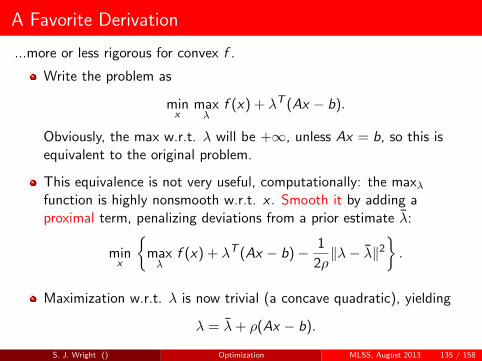

A Favorite Derivation (Cont.)
Inserting λ = λ+ ρ(Ax − b) leads to
minx
f (x) + λT (Ax − b) +ρ
2‖Ax − b‖2 = L(x , λ; ρ).
Hence can view the augmented Lagrangian process as:
X minx L(x , λ; ρ) to get new x ;
X Shift the “prior” on λ by updating to the latest max: λ+ ρ(Ax − b);
X Increase ρk if not happy with improvement in feasibility;
X repeat until convergence.
Add subscripts, and we recover the augmented Lagrangian algorithm ofthe first slide!
S. J. Wright () Optimization MLSS, August 2013 136 / 158

Inequality Constraints
The same derivation can be used for inequality constraints:
min f (x) s.t. Ax ≥ b.
Apply the same reasoning to the constrained min-max formulation:
minx
maxλ≥0
f (x)− λT (Ax − b).
After the prox-term is added, can find the minimizing λ in closed form(as for prox-operators). Leads to update formula:
λ← max(λ+ ρ(Ax − b), 0
).
This derivation extends immediately to nonlinear constraintsc(x) = 0 or c(x) ≥ 0.
S. J. Wright () Optimization MLSS, August 2013 137 / 158

“Explicit” Constraints, Inequality Constraints
There may be other constraints on x (such as x ∈ Ω) that we preferto handle explicitly in the subproblem.
For the formulation minx
f (x), s.t. Ax = b, x ∈ Ω,
the minx step can enforce x ∈ Ω explicitly:
xk = arg minx∈ΩL(x , λk−1; ρ);
λk = λk−1 + ρ(Axk − b);
This gives an alternative way to handle inequality constraints:introduce slacks s, and enforce them explicitly. That is, replace
minx
f (x) s.t. c(x) ≥ 0,
byminx ,s
f (x) s.t. c(x) = s, s ≥ 0,
and enforce s ≥ 0 explicitly in the subproblems.
S. J. Wright () Optimization MLSS, August 2013 138 / 158

Quick History of Augmented Lagrangian
Dates from at least 1969: Hestenes, Powell.
Developments in 1970s, early 1980s by Rockafellar, Bertsekas, andothers.
Lancelot code for nonlinear programming (Conn et al., 1992).
Lost favor somewhat as an approach for general nonlinearprogramming during the next 15 years.
Recent revival in the context of sparse optimization and its manyapplications, in conjunction with splitting / coordinate descent.
S. J. Wright () Optimization MLSS, August 2013 139 / 158

Alternating Direction Method of Multipliers (ADMM)
Consider now problems with a separable objective of the form
min(x ,z)
f (x) + h(z) s.t. Ax + Bz = c ,
for which the augmented Lagrangian is
L(x , z , λ; ρ) := f (x) + h(z) + λT (Ax + Bz − c) +ρ
2‖Ax − Bz − c‖2
2.
Standard AL would minimize L(x , z , λ; ρ) w.r.t. (x , z) jointly.However, these are coupled in the quadratic term, separability is lost
In ADMM, minimize over x and z separately and sequentially:
xk = arg minxL(x , zk−1, λk−1; ρk);
zk = arg minzL(xk , z , λk−1; ρk);
λk = λk−1 + ρk(Axk + Bzk − c).
S. J. Wright () Optimization MLSS, August 2013 140 / 158
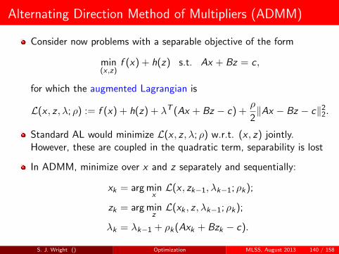
Alternating Direction Method of Multipliers (ADMM)
Consider now problems with a separable objective of the form
min(x ,z)
f (x) + h(z) s.t. Ax + Bz = c ,
for which the augmented Lagrangian is
L(x , z , λ; ρ) := f (x) + h(z) + λT (Ax + Bz − c) +ρ
2‖Ax − Bz − c‖2
2.
Standard AL would minimize L(x , z , λ; ρ) w.r.t. (x , z) jointly.However, these are coupled in the quadratic term, separability is lost
In ADMM, minimize over x and z separately and sequentially:
xk = arg minxL(x , zk−1, λk−1; ρk );
zk = arg minzL(xk , z , λk−1; ρk );
λk = λk−1 + ρk (Axk + Bzk − c).
S. J. Wright () Optimization MLSS, August 2013 140 / 158
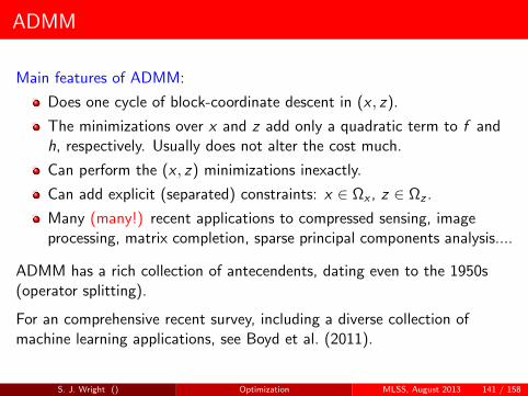
ADMM
Main features of ADMM:
Does one cycle of block-coordinate descent in (x , z).
The minimizations over x and z add only a quadratic term to f andh, respectively. Usually does not alter the cost much.
Can perform the (x , z) minimizations inexactly.
Can add explicit (separated) constraints: x ∈ Ωx , z ∈ Ωz .
Many (many!) recent applications to compressed sensing, imageprocessing, matrix completion, sparse principal components analysis....
ADMM has a rich collection of antecendents, dating even to the 1950s(operator splitting).
For an comprehensive recent survey, including a diverse collection ofmachine learning applications, see Boyd et al. (2011).
S. J. Wright () Optimization MLSS, August 2013 141 / 158

ADMM: A Simpler Form
Often, a simpler version is enough: min(x ,z)
f (x) + h(z) s.t. Ax = z ,
equivalent to minx
f (x) + h(Ax), often the one of interest.
In this case, the ADMM can be written as
xk = arg minx
f (x) + ρ2‖A x − zk−1 − dk−1‖2
2
zk = arg minz
h(z) + ρ2‖A xk−1 − z − dk−1‖2
2
dk = dk−1 − (A xk − zk)
the so-called “scaled version” (Boyd et al., 2011).
Updating zk is a proximity computation: zk = proxh/ρ
(A xk−1− dk−1
)Updating xk may be hard: if f is quadratic, involves matrix inversion;if f is not quadratic, may be as hard as the original problem.
S. J. Wright () Optimization MLSS, August 2013 142 / 158

ADMM: A Simpler Form
Often, a simpler version is enough: min(x ,z)
f (x) + h(z) s.t. Ax = z ,
equivalent to minx
f (x) + h(Ax), often the one of interest.
In this case, the ADMM can be written as
xk = arg minx
f (x) + ρ2‖A x − zk−1 − dk−1‖2
2
zk = arg minz
h(z) + ρ2‖A xk−1 − z − dk−1‖2
2
dk = dk−1 − (A xk − zk )
the so-called “scaled version” (Boyd et al., 2011).
Updating zk is a proximity computation: zk = proxh/ρ
(A xk−1− dk−1
)
Updating xk may be hard: if f is quadratic, involves matrix inversion;if f is not quadratic, may be as hard as the original problem.
S. J. Wright () Optimization MLSS, August 2013 142 / 158

ADMM: A Simpler Form
Often, a simpler version is enough: min(x ,z)
f (x) + h(z) s.t. Ax = z ,
equivalent to minx
f (x) + h(Ax), often the one of interest.
In this case, the ADMM can be written as
xk = arg minx
f (x) + ρ2‖A x − zk−1 − dk−1‖2
2
zk = arg minz
h(z) + ρ2‖A xk−1 − z − dk−1‖2
2
dk = dk−1 − (A xk − zk )
the so-called “scaled version” (Boyd et al., 2011).
Updating zk is a proximity computation: zk = proxh/ρ
(A xk−1− dk−1
)Updating xk may be hard: if f is quadratic, involves matrix inversion;if f is not quadratic, may be as hard as the original problem.
S. J. Wright () Optimization MLSS, August 2013 142 / 158

ADMM: Convergence
Consider the problem minx
f (x) + h(Ax), where f and h are lower
semi-continuous, proper, convex functions and A has full column rank.
The ADMM algorithm presented in the previous slide converges (forany ρ > 0) to a solution x∗, if one exists, otherwise it diverges.
This is a cornerstone result by Eckstein and Bertsekas (1992).
As in IST/FBS/PGA, convergence is still guaranteed with inexactlysolved subproblems, as long as the errors are absolutely summable.
The recent burst of interest in ADMM is evident from the citationrecord of Eckstein and Bertsekas (1992).
S. J. Wright () Optimization MLSS, August 2013 143 / 158

Special Case: `2-`1
Standard problem: minx12‖Ax − b‖2
2 + ‖x‖1. ADMM becomes
xk = arg minx‖x‖1 + ρ
2‖A x − zk−1 − dk−1‖22
zk = arg minz
h(z) + ρ2‖A xk−1 − z − dk−1‖2
2
dk = dk−1 − (A xk − zk )
Subproblems are
xk := (AT A + ρk I )−1(AT b + ρk zk−1 − λk ),
zk := minz
τ‖z‖1 + (λk )T (xk − z) +ρk
2‖z − xk‖2
2
= proxτ/ρk(xk + λk/ρk )
λk+1 := λk + ρk (xk − zk ).
Solving for xk is the most complicated part of the calculation. If theleast-squares part is underdetermined (A is m × n with n > m), can makeuse of the Sherman-Morrison-Woodbury formula:
(AT A + ρk I )−1 =1
ρkI − 1
ρkAT (ρk I + AAT )−1A,
where the inner matrix has size m ×m (smaller than n × n).
S. J. Wright () Optimization MLSS, August 2013 144 / 158

Moreover, in some compressed sensing applications, we have AAT = I . Inthis case, xk can be recovered at the cost of two matrix-vectormultiplications involving A.
Otherwise, can solve for xk inexactly, using a few steps of an iterativemethod.
The YALL1 code solves this problem, and other problems with moregeneral regularizers (e.g. groups).
S. J. Wright () Optimization MLSS, August 2013 145 / 158

ADMM for Sparse Inverse Covariance
maxX0
log det(X )− 〈X ,S〉 − τ‖X‖1,
Reformulate as
maxX0
log det(X )− 〈X , S〉 − τ‖Z‖1 s.t. X − Z = 0.
Subproblems are:
Xk := arg maxX
log det(X )− 〈X , S〉 − 〈Uk−1,X − Zk−1〉
− ρk
2‖X − Zk−1‖2
F
:= arg maxX
log det(X )− 〈X , S〉 − ρk
2‖X − Zk−1 + Uk/ρk‖2
F
Zk := proxτ/ρk‖·‖1(Xk + Uk );
Uk+1 := Uk + ρk (Xk − Zk ).
S. J. Wright () Optimization MLSS, August 2013 146 / 158

Solving for X
Get optimality condition for the X subproblem by using∇X log det(X ) = X−1, when X is s.p.d. Thus,
X−1 − S − ρk (X − Zk−1 + Uk/ρk ) = 0,
which is equivalent to
X−1 − ρk X − (S − ρk Zk−1 + Uk ) = 0.
Form eigendecomposition
(S − ρk Zk−1 + Uk ) = QΛQT ,
where Q is n × n orthogonal and Λ is diagonal with elements λi . Seek Xwith the form QΛQT , where Λ has diagonals λi . Must have
1
λi
− ρk λi − λi = 0, i = 1, 2, . . . , n.
Take positive roots: λi = [λi +√λ2
i + 4ρk ]/(2ρk ), i = 1, 2, . . . , n.
S. J. Wright () Optimization MLSS, August 2013 147 / 158

VI. Coordinate Descent
Consider first min f (x) with f : Rn → R.
Iteration j of basic coordinate descent:
Choose index ij ∈ 1, 2, . . . , n;Fix all components i 6= ij , change xij in a way that (hopefully) reducesf .
Variants for the reduced step:
take a reduced gradient step: −∇ij f (x);
do a more rigorous search in the subspace defined by ij ;
actually minimize f in the ij component.
Many extensions of this basic idea.
An old approach, revived recently because of useful applications in machinelearning, and interesting possibilities as stochastic and parallel algorithms.
S. J. Wright () Optimization MLSS, August 2013 148 / 158

Block Coordinate Descent
At iteration j , choose a subset Gj ⊂ 1, 2, . . . , n and allow only thecomponents in Gj to change. Fix the components xi for i /∈ Gj .
Again, the step could be a reduced gradient step along −∇Gjf (x), or a
more elaborate search.
There are many different heuristics for choosing Gj , often arising naturallyfrom the application.
Constraints and regularizers complicate things! Make block partitionconsistent with separablity of constraints / regularizers.
S. J. Wright () Optimization MLSS, August 2013 149 / 158

Deterministic and Stochastic CD
Stepxj+1,ij = xj ,ij − αj [∇f (xj )]ij .
Deterministic CD: choose ik in some fixed order e.g. cyclic;
Stochastic CD: choose ik at random from 1, 2, . . . , n.
CD is a reasonable choice when it’s cheap to evaluate individual elementsof ∇f (x) (e.g. at 1/n of the cost of a full gradient, say).
Convergence: Deterministic (Luo and Tseng, 1992; Tseng, 2001), linearrate (Beck and Tetruashvili, 2013). Stochastic, linear rate: (Nesterov,2012).
S. J. Wright () Optimization MLSS, August 2013 150 / 158

Coordinate Descent in Dual SVM
Coordinate descent has long been popular for solving the dual (QP)formulation of support vector machines.
minα∈RN
1
2αT Kα− 1Tα s.t. 0 ≤ α ≤ C1, y Tα = 0.
SMO: Each Gk has two components. (Thus can maintain feasibilitywith respect to the single linear constraint y Tα = 0.)
LIBSVM: SMO approach (still |Gk | = 2), with different heuristic.
LASVM: Again |Gk | = 2, with focus on online setting.
SVM-light: Small |Gk | (default 10).
GPDT: Larger |Gk | (default 400) with gradient projection solver asthe subproblem solver.
S. J. Wright () Optimization MLSS, August 2013 151 / 158

Asynchronous Stochastic Coordinate Descent (ASCD)
Consider min f (x), where f : Rn → Rn is smooth and convex.
Each processor (independently, without synchronization) does:
1. Choose i ∈ 1, 2, . . . , n uniformly at random;
2. Read x and evaluate g = [∇f (x)]i ;
3. Update xi ← xi − γLmax
g ;
Here γ is a steplength (more below) and Lmax is a bound on the diagonalsof the Hessian ∇2f (x).
Assume that not more than τ cycles pass between when x is read (step 2)and updated (step 3).
How to choose γ to achieve good convergence?
S. J. Wright () Optimization MLSS, August 2013 152 / 158

Constants and “Diagonalicity”
Several constants are critical to the analysis.
τ : maximum delay;
Lmax: maximum diagonal of ∇2f (x);
Lres: maximum row norm of Hessian;
µ: lower bound on eigenvalues of ∇2f (x) (assumed positive).
The ratio Lres/Lmax is particularly important — it measures the degree ofdiagonal dominance in the Hessian ∇2f (x) (Diagonalicity).
By convexity, we have
1 ≤ Lres
Lmax≤√
n.
Closer to 1 if Hessian is nearly diagonally dominant (eigenvectors close toprincipal coordinate axes). Smaller is better for parallelism.
S. J. Wright () Optimization MLSS, August 2013 153 / 158

Diagonalicity Illustrated
Left figure is better. It can tolerate a higher delay parameter τ and thusmore cores working asynchronously.
S. J. Wright () Optimization MLSS, August 2013 154 / 158

How to choose γ?
Choose some ρ > 1 and pick γ small enough to ensure that
ρ−1 ≤E(‖∇f (xj+1)‖2)
E(‖∇f (xj )‖2)≤ ρ.
Not too much change in gradient over each iteration, so not too muchprice to pay for using old information, in the asynchronous setting.
Choose γ small enough to satisfy this property but large enough to get alinear rate.
Assuming that
τ + 1 ≤√
nLmax
2eLres,
and choosing ρ = 1 + 2eLres√nLmax
, we can take γ = 1. Then have
E(f (xj )− f ∗) ≤(
1− µ
2nLmax
)j
(f (x0)− f ∗).
(Liu and Wright, 2013)S. J. Wright () Optimization MLSS, August 2013 155 / 158

ASCD Discussion
Linear rate is close to the rate attained by short-step steepest descent.
Bound on τ is a measure of potential parallelization. When ratio Lres/Lmax
is favorable, get τ = O(√
n). Thus, expect near-linear speedup on toO(√
n) cores running asynchronously in parallel.
Can extend algorithm and analysis to
“Essentially strongly convex” and “weakly convex” cases;
Separable constraints. Have τ = O(n1/4) — less potential parallelism.
S. J. Wright () Optimization MLSS, August 2013 156 / 158

Implemented on 4-socket, 40-core Intel Xeon
minx
‖Ax − b‖2 + 0.5‖x‖2
where A ∈ Rm×n is a Gaussian random matrix (m = 6000, n = 20000,columns are normalized to 1). Lres/Lmax ≈ 2.2. Choose γ = 1.
0 5 10 15 20 25 30
# epochs10-5
10-4
10-3
10-2
10-1
100
101
102
resi
dual
t=1t=2t=4t=8t=16t=32
0 5 10 15 20 25 30 35 40
threads0
5
10
15
20
25
30
35
40
spee
dup
idealobserved
(Thanks: C. Re, V. Bittorf, S. Sridhar)S. J. Wright () Optimization MLSS, August 2013 157 / 158

Conclusions
We’ve seen a sample of optimization tools that are relevant tolearning, as currently practiced.
Many holes in this discussion! Check the “matching” slides at thestart for further leads.
Besides being a source of algorithmic tools, optimization offers someinteresting perspectives on formulation.
Optimizers get a lot of brownie points for collaborating with learningand data analysis researchers, so don’t hesitate to talk to us!
S. J. Wright () Optimization MLSS, August 2013 158 / 158
References I
Akaike, H. (1959). On a successive transformation of probability distribution and its applicationto the analysis fo the optimum gradient method. Annals of the Institute of Statistics andMathematics of Tokyo, 11:1–17.
Amaldi, E. and Kann, V. (1998). On the approximation of minimizing non zero variables orunsatisfied relations in linear systems. Theoretical Computer Science, 209:237–260.
Bach, F., Jenatton, R., Mairal, J., and Obozinski, G. (2012). Structured sparsity throughconvex optimization. Statistical Science, 27:450–468.
Barzilai, J. and Borwein, J. (1988). Two point step size gradient methods. IMA Journal ofNumerical Analysis, 8:141–148.
Beck, A. and Teboulle, M. (2009a). A fast iterative shrinkage-thresholding algorithm for linearinverse problems. SIAM Journal on Imaging Sciences, 2(1):183–202.
Beck, A. and Teboulle, M. (2009b). A fast iterative shrinkage-threshold algorithm for linearinverse problems. SIAM Journal on Imaging Sciences, 2(1):183–202.
Beck, A. and Tetruashvili, L. (2013). On the convergence of block coordinate descent methods.Technical report, Technion-Israel Institute of Technology.
Bottou, L. (2012). leon.bottou.org/research/stochastic.
Bottou, L. and LeCun, Y. (2004). Large-scale online learning. In Advances in NeuralInformation Processing Systems.
S. J. Wright () Optimization MLSS, August 2013 1 / 11

References II
Boyd, S., Parikh, N., Chu, E., Peleato, B., and Eckstein, J. (2011). Distributed optimizationand statistical learning via the alternating direction method of multipliers. Foundations andTrends in Machine Learning, 3(1):1–122.
Byrd, R. H., Chin, G. M., Neveitt, W., and Nocedal, J. (2011). On the use of stochastic hessianinformation in unconstrained optimization. SIAM Journal on Optimization, 21:977–995.
Cai, J.-F., Candes, E., and Shen, Z. (2010a). A singular value thresholding algorithm for matrixcompletion. SIAM Journal on Optimization, 20(4).
Cai, J.-F., Candes, E., and Shen, Z. (2010b). A singular value thresholding algorithm for matrixcompletion. SIAM JOurnal on Optimization, 20:1956–1982.
Candes, E. and Romberg, J. (2005). `1-MAGIC: Recovery of sparse signals via convexprogramming. Technical report, California Institute of Technology.
Candes, E., Romberg, J., and Tao, T. (2006a). Robust uncertainty principles: Exact signalreconstruction from highly incomplete frequency information. IEEE Transactions onInformation Theory, 52:489–509.
Candes, E., Romberg, J., and Tao, T. (2006b). Stable signal recovery from incomplete andinaccurate measurements. Communications in Pure and Applied Mathematics, 59:1207–1223.
Caruana, R. (1997). Multitask learning. Machine Learning, 28(1):41–75.
Chan, T. F., Golub, G. H., and Mulet, P. (1999). A nonlinear primal-dual method for totalvariation based image restoration. SIAM Journal of Scientific Computing, 20:1964–1977.
S. J. Wright () Optimization MLSS, August 2013 2 / 11

References III
Chang, C.-C. and Lin, C. (2011). LIBSVM: a library for support vector machines. ACMTransactions on Intelligent Systems and Technology, 2.
Chen, S., Donoho, D., and Saunders, M. (1995). Atomic decomposition by basis pursuit.Technical report, Department of Statistics, Stanford University.
Combettes, P. and Pesquet, J.-C. (2011). Signal recovery by proximal forward-backwardsplitting. In Fixed-Point Algorithms for Inverse Problems in Science and Engineering, pages185–212. Springer.
Combettes, P. and Wajs, V. (2006). Proximal splitting methods in signal processing. MultiscaleModeling and Simulation, 4:1168–1200.
Conn, A., Gould, N., and Toint, P. (1992). LANCELOT: a Fortran package for large-scalenonlinear optimization (Release A). Springer Verlag, Heidelberg.
d’Aspremont, A., Banerjee, O., and El Ghaoui, L. (2008). First-order methods for sparsecovariance selection. SIAM Journal on Matrix Analysis and Applications, 30:56–66.
Davis, G., Mallat, S., and Avellaneda, M. (1997). Greedy adaptive approximation. Journal ofConstructive Approximation, 13:57–98.
Dekel, O., Gilad-Bachrach, R., Shamir, O., and Xiao, L. (2012). Optimal distributed onlineprediction using mini-batches. Journal of Machine Learning Research, 13:165–202.
Donoho, D. (2006). Compressed sensing. IEEE Transactions on Information Theory,52:1289–1306.
S. J. Wright () Optimization MLSS, August 2013 3 / 11

References IV
Duchi, J., Agarwal, A., and Wainwright, M. J. (2010). Distributed dual averaging in networks.In Advances in Neural Information Processing Systems.
Duchi, J. and Singer, Y. (2009). Efficient learning using forward-backward splitting. InAdvances in Neural Information Processing Systems. http://books.nips.cc.
Eckstein, J. and Bertsekas, D. (1992). On the Douglas-Rachford splitting method and theproximal point algorithm for maximal monotone operators. Mathematical Programming,5:293–318.
Efron, B., Hastie, T., Johnstone, I., and Tibshirani, R. (2004). Least angle regression. Annals ofStatistics, 32(2):407–499.
Ferris, M. C. and Munson, T. S. (2002). Interior-point methods for massive support vectormachines. SIAM Journal on Optimization, 13(3):783–804.
Figueiredo, M. A. T. and Nowak, R. D. (2003). An EM algorithm for wavelet-based imagerestoration. IEEE Transactions on Image Processing, 12:906–916.
Fine, S. and Scheinberg, K. (2001). Efficient svm training using low-rank kernel representations.Journal of Machine Learning Research, 2:243–264.
Fountoulakis, K. and Gondzio, J. (2013). A second-order method for strongly convexell1-regularization problems. Technical Report ERGO-13-011, University of Edinburgh.
Fountoulakis, K., Gondzio, J., and Zhlobich, P. (2012). Matrix-free interior point method forcompressed sensing problems. Technical Report, University of Edinburgh.
S. J. Wright () Optimization MLSS, August 2013 4 / 11

References V
Friedman, J., Hastie, T., and Tibshirani, R. (2008). Sparse inverse covariance estimation withthe graphical lasso. Biostatistics, 9(3):432–441.
Garnaev, A. and Gluskin, E. (1984). The widths of an Euclidean ball. Doklady Akademii Nauk,277:1048–1052.
Gertz, E. M. and Wright, S. J. (2003). Object-oriented software for quadratic programming.ACM Transations on Mathematical Software, 29:58–81.
Goldfarb, D., Ma, S., and Scheinberg, K. (2012). Fast alternating linearization methods forminimizing the sum of two convex functions. Mathematical Programming, Series A. DOI10.1007/s10107-012-0530-2.
Gondzio, J. and Fountoulakis, K. (2013). Second-order methods for l1-regularization. Talk atOptimization and Big Data Workshop, Edinburgh.
Hale, E., Yin, W., and Zhang, Y. (2008). Fixed-point continuation for l1-minimization:Methodology and convergence. SIAM Journal on Optimization, 19:1107–1130.
Haupt, J. and Nowak, R. (2006). Signal reconstruction from noisy random projections. IEEETransactions on Information Theory, 52:4036–4048.
Hestenes, M. (1969). Multiplier and gradient methods. Journal of Optimization Theory andApplications, 4:303–320.
Hinton, G. E., Osindero, S., and Teh, Y.-W. (2006). A fast learning algorithm for deep beliefnets. Neural Computation, 18(7):1527–1554.
S. J. Wright () Optimization MLSS, August 2013 5 / 11

References VI
Jaggi, M. (2013). Revisiting frank-wolfe: Projection-free sparse convex optimization. InProceedings of ICML 2013.
Joachims, T. (1999). Making large-scale support vector machine learning practical. InScholkopf, B., Burges, C., and Smola, A., editors, Advances in Kernel Methods - SupportVector Learning, chapter 11, pages 169–184. MIT Press, Cambridge, MA.
Kashin, B. (1977). Diameters of certain finite-dimensional sets in classes of smooth functions.Izvestiya Akademii Nauk. SSSR: Seriya Matematicheskaya, 41:334–351.
Langford, J., Li, L., and Zhang, T. (2009). Sparse online learning via truncated gradient.Journal of Machine Learning Research, 10:777–801.
Le, Q. V., Ranzato, M., Monga, R., Devin, M., Chen, K., Corrado, G. S., Dean, J., and Ng,A. Y. (2012). Building high-level features using large scale unsupervised learning. InProceedings of the Conference on Learning Theory. arXiv:1112.6209v5.
Lee, J., Recht, B., Salakhutdinov, R., Srebro, N., and Tropp, J. (2010). Practical large-scaleoptimization for max-norm regularization. In Advances in Neural Information ProcessingSystems. NIPS.
Lee, S. and Wright, S. J. (2012). Manifold identification in dual averaging methods forregularized stochastic online learning. Journal of Machine Learning Research, 13:1705–1744.
Lee, S. I., Lee, H., Abbeel, P., and Ng, A. Y. (2006). Efficient `1 regularized logistic regerssion.In Proceedings of the National Conference of the American Association for ArtificialIntelligence.
S. J. Wright () Optimization MLSS, August 2013 6 / 11

References VII
Lin, C., Weng, R. C., and Keerthi, S. S. (2008). Trust-region newton method for logisticregression. Journal of Machine Learning Research, 9:627–650.
Liu, D. C. and Nocedal, J. (1989). On the limited-memory BFGS method for large scaleoptimization. Mathematical Programming, Series A, 45:503–528.
Liu, J. and Wright, S. J. (2013). An asynchronous parallel stochastic coordinate descentmethod. In preparation.
Luo, Z. Q. and Tseng, P. (1992). On the convergence of the coordinate descent method forconvex differentiable minimization. Journal of Optimization Theory and Applications,72(1):7–35.
Ma, S., Goldfarb, D., and Chen, L. (2011). Fixed point and Bregman iterative methods formatrix rank minimization. Mathematical Programming (Series A), 128:321–353.
Martens, J. (2010). Deep learning via Hessian-free optimization. In Proceedings of the 27thInternational Conference on Machine Learning.
Martins, A. F. T., Smith, N. A., Aguiar, P. M. Q., and Figueiredo, M. A. T. (2011). StructuredSparsity in Structured Prediction. In Proc. of Empirical Methods for Natural LanguageProcessing.
Meier, L., van de Geer, S., and Buhlmann, P. (2008). The group lasso for logistic regression.Journal of the Royal Statistical Society B, 70(1):53–71.
Moreau, J. (1962). Fonctions convexes duales et points proximaux dans un espace hilbertien.CR Acad. Sci. Paris Ser. A Math, 255:2897–2899.
S. J. Wright () Optimization MLSS, August 2013 7 / 11
References VIII
Muthukrishnan, S. (2005). Data Streams: Algorithms and Applications. Now Publishers,Boston, MA.
Nemirovski, A., Juditsky, A., Lan, G., and Shapiro, A. (2009). Robust stochastic approximationapproach to stochastic programming. SIAM Journal on Optimization, 19(4):1574–1609.
Nesterov, Y. (1983). A method of solving a convex programming problem with convergence rateO(1/k2). Soviet Math. Doklady, 27:372–376.
Nesterov, Y. (2012). Efficiency of coordinate descent methods on huge-scale optimizationproblems. SIAM Journal on Optimization, 22:341–362.
Niu, F., Recht, B., Re, C., and Wright, S. J. (2011). Hogwild!: A lock-free approach toparallelizing stochastic gradient descent. In Advances in Neural Information ProcessingSystems.
Nocedal, J. and Wright, S. J. (2006). Numerical Optimization. Springer, New York.
Obozinski, G., Taskar, B., and Jordan, M. (2010). Joint covariate selection and joint subspaceselection for multiple classification problems. Statistics and Computing, 20(2):231–252.
Platt, J. C. (1999). Fast training of support vector machines using sequential minimaloptimization. In Scholkopf, B., Burges, C. J. C., and Smola, A. J., editors, Advances inKernel Methods — Support Vector Learning, pages 185–208, Cambridge, MA. MIT Press.
Powell, M. (1969). A method for nonlinear constraints in minimization problems. In Fletcher,R., editor, Optimization, pages 283–298. Academic Press, New York.
S. J. Wright () Optimization MLSS, August 2013 8 / 11

References IX
Recht, B., Fazel, M., and Parrilo, P. (2010). Guaranteed minimum-rank solutions of linearmatrix equations via nuclear norm minimization. SIAM Review, 52:471–501.
Richtarik, P. (2012). Hogwild! and other hybrid beasts. Notes.
Scheinberg, K. and Ma, S. (2012). Optimization methods for sparse inverse covarianceselection. In Sra, S., Nowozin, S., and Wright, S. J., editors, Optimization for MachineLearning, Neural Information Processing Series. MIT Press.
Schmidt, M. and Murphy, K. (2010). Convex structure learning in log-linear models: Beyondpairwise potentials. In Proc. of AISTATS.
Shalev-Shwartz, S., Singer, Y., and Srebro, N. (2007). Pegasos: Primal Estimated sub-GrAdientSOlver for SVM. In Proceedings of the 24th International Confernece on Machine Learning.
Shevade, S. K. and Keerthi, S. S. (2003). A simple and efficient algorithm for gene selectionusing sparse logistic regression. Bioinformatics, 19(17):2246–2253.
Shi, W., Wahba, G., Wright, S. J., Lee, K., Klein, R., and Klein, B. (2008).LASSO-Patternsearch algorithm with application to opthalmology data. Statistics and itsInterface, 1:137–153.
Srebro, N. and Tewari, A. (2010). Stochastic optimization for machine learning. Tutorial, ICML2010, Haifa, Israel.
Stojnic, M., Parvaresh, F., and Hassibi, B. (2009). On the reconstruction of block-sparse signalswith an optimal number of measurements. Signal Processing, IEEE Transactions on,57(8):3075–3085.
S. J. Wright () Optimization MLSS, August 2013 9 / 11
References X
Tibshirani, R. (1996). Regression shrinkage and selection via the lasso. Journal of the RoyalStatistical Society B., pages 267–288.
Tillmann, A. and Pfetsch, M. (2012). The computational complexity of RIP, NSP, and relatedconcepts in compressed sensing. Technical report, arXiv/1205.2081.
Tseng, P. (2001). Convergence of a block coordinate descent method for nondifferentiableminimization. Journal of Optimization Theory and Applications, 109(3):475–494.
Turlach, B., Venables, W. N., and Wright, S. J. (2005). Simultaneous variable selection.Technometrics, 47(3):349–363.
Wen, Z., Yin, W., Goldfarb, D., and Zhang, Y. (2010). A fast algorithms for sparsereconstruction based on shrinkage, subspace optimization, and continuation. SIAM Journalon Scientific Computing, 32(4):1832–1857.
Wen, Z., Yin, W., and Zhang, Y. (2012). Solving a low-rank factorization model for matrixcompletion by a nonlinear successive over-relaxation algorithm. Mathematical ProgrammingComputation, 4:333–361.
Wright, S., Nowak, R., and Figueiredo, M. (2009a). Sparse reconstruction by separableapproximation. IEEE Transactions on Signal Processing, 57:2479–2493.
Wright, S. J. (1997). Primal-Dual Interior-Point Methods. SIAM, Philadelphia, PA.
Wright, S. J., Nowak, R. D., and Figueiredo, M. A. T. (2009b). Sparse reconstruction byseparable approximation. IEEE Transactions on Signal Processing, 57:2479–2493.
S. J. Wright () Optimization MLSS, August 2013 10 / 11

References XI
Xiao, L. (2010). Dual averaging methods for regularized stochastic learning and onlineoptimization. Journal of Machine Learning Research, 11:2543–2596.
Xiao, L. and Zhang, T. (2012). A proximal-gradient homotopy method for the sparseleast-squares problem. SIAM Journal on Optimization. (to appear; available athttp://arxiv.org/abs/1203.3002).
Yin, W., Osher, S., Goldfarb, D., and Darbon, J. (2008). Bregman iterative algorithms for`1-minimization with applications to compressed sensing. SIAM Journal on Imaging Sciences,1(1):143–168.
Yin, W. and Zhang, Y. (2008). Extracting salient features from less data via `1-minimizationauthors. SIAG/OPT Views-and-News, 19:11–19.
Zhang, Y., Yang, J., and Yin, W. (2010). User’s guide for YALL1: Your algorithms for L1optimization. CAAM Technical Report TR09-17, CAAM Department, Rice University.
Zhao, P., Rocha, G., and Yu, B. (2009). Grouped and hierarchical model selection throughcomposite absolute penalties. Annals of Statistics, 37(6A):3468–3497.
Zhu, M., Wright, S. J., and Chan, T. F. (2010). Duality-based algorithms for total variationimage restoration. Computational Optimization and Applications, 47(3):377–400. DOI:10.1007/s10589-008-9225-2.
Zinkevich, M. (2003). Online convex programming and generalized infinitesimal gradient ascent.In Proceedings of the 20th International Conference on Machine Learning, pages 928–936.
S. J. Wright () Optimization MLSS, August 2013 11 / 11