optimizacijske metode / razvr canje v skupine · v. batagelj: optimizacijske metode / 9....

'

&

$

%na vrhu

Optimizacijske metode9. razvrscanjev skupineVladimir Batagelj

Univerza v LjubljaniFMF, matematika

razlicica: 31. maj 2013 / 09 : 34

V. Batagelj: Optimizacijske metode / 9. razvrscanje v skupine 1'

&

$

%

Kazalo1 Clustering . . . . . . . . . . . . . . . . . . . . . . . . . . . . . 1

2 Basic notions . . . . . . . . . . . . . . . . . . . . . . . . . . . 2

3 Clustering problem . . . . . . . . . . . . . . . . . . . . . . . . 3

4 Units . . . . . . . . . . . . . . . . . . . . . . . . . . . . . . . . 4

5 Clusterings . . . . . . . . . . . . . . . . . . . . . . . . . . . . 5

6 Simple criterion functions . . . . . . . . . . . . . . . . . . . . . 6

7 Cluster-error function / dissimilarities . . . . . . . . . . . . . . 7

8 Properties of dissimilarities . . . . . . . . . . . . . . . . . . . . 8

16 Cluster-error function / examples . . . . . . . . . . . . . . . . . 16

18 Sensitive criterion functions . . . . . . . . . . . . . . . . . . . 18

19 Representatives . . . . . . . . . . . . . . . . . . . . . . . . . . 19

22 Other criterion functions . . . . . . . . . . . . . . . . . . . . . 22

Univerza v Ljubljani s s y s l s y ss * 6


&

$

%

25 Complexity of the clustering problem . . . . . . . . . . . . . . 25

26 Complexity results . . . . . . . . . . . . . . . . . . . . . . . . 26

31 Approaches to Clustering . . . . . . . . . . . . . . . . . . . . . 31

32 Local optimization . . . . . . . . . . . . . . . . . . . . . . . . 32

33 Local optimization . . . . . . . . . . . . . . . . . . . . . . . . 33

38 Dynamic programming . . . . . . . . . . . . . . . . . . . . . . 38

39 Hierarchical methods . . . . . . . . . . . . . . . . . . . . . . . 39

54 About the minimal solutions of (Pk,SR) . . . . . . . . . . . . . 54

56 Leaders method . . . . . . . . . . . . . . . . . . . . . . . . . . 56

57 The dynamic clusters method . . . . . . . . . . . . . . . . . . . 57

64 Clustering and Networks . . . . . . . . . . . . . . . . . . . . . 64

65 Clustering with relational constraint . . . . . . . . . . . . . . . 65

69 Neighborhood Graphs . . . . . . . . . . . . . . . . . . . . . . . 69



&

$

%

72 Clustering of Graphs and Networks . . . . . . . . . . . . . . . 72

77 Clustering in Graphs and Networks . . . . . . . . . . . . . . . . 77

81 Graph theory approaches . . . . . . . . . . . . . . . . . . . . . 81

90 Final remarks . . . . . . . . . . . . . . . . . . . . . . . . . . . 90



&

$

%

Clustering• basic notions: cluster, clustering, feasible clustering, criterion function,

dissimilarities, clustering as an optimization problem

• different (nonstandard) problems: assignment of students to classes,regionalization; general criterion function; multicriteria problems.

• complexity results about the clustering problem – NP-hardness theo-rems



&

$

%

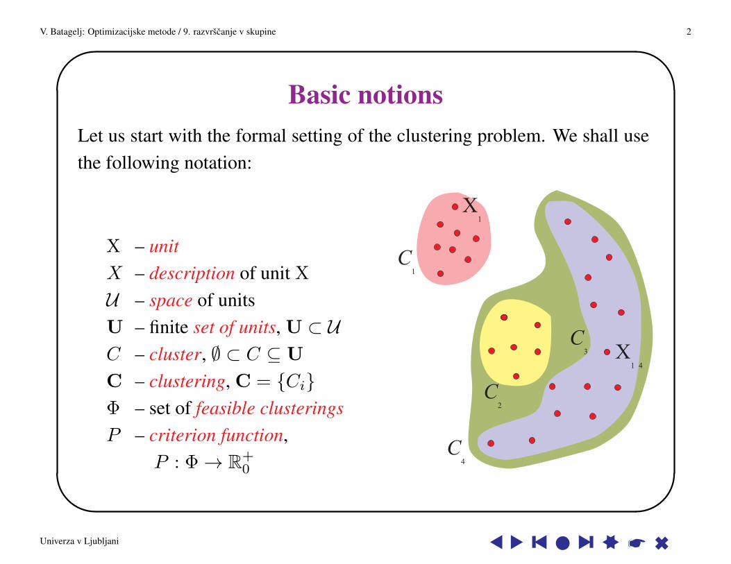
Basic notionsLet us start with the formal setting of the clustering problem. We shall usethe following notation:

X – unitX – description of unit X

U – space of unitsU – finite set of units, U ⊂ UC – cluster, ∅ ⊂ C ⊆ U

C – clustering, C = {Ci}Φ – set of feasible clusteringsP – criterion function,

P : Φ→ R+0



&

$

%

Clustering problemWith these notions we can express the clustering problem (Φ, P ) as follows:

Determine the clustering C? ∈ Φ for which

P (C?) = minC∈Φ

P (C)

Since the set of units U is finite, the set of feasible clusterings is alsofinite. Therefore the set Min(Φ, P ) of all solutions of the problem (optimalclusterings) is not empty. (In theory) the set Min(Φ, P ) can be determinedby the complete search.

We shall denote the value of criterion function for an optimal clustering bymin(Φ, P ).



&

$

%

Unitsreal or imaginary objects of analysis

WORLD UNITS DESCRIPTIONS

{X} ←→ X ←→ [X]

formalization operationalization

{ produced cars T } car T [ seats=4, max-speed= . . . ]

Usually an unit X is represented by a vector/description X ≡ [X] =

[x1, x2, ..., xm] from the set [U ] of all possible descriptions. xi = Vi(X)

is the value of the i-th of selected properties or variables on X. Variablescan be measured in different scales: nominal, ordinal, interval, rational,absolute (Roberts, 1976).

There exist other kinds of descriptions of units: symbolic object (Bock,Diday, 2000), list of keywords from a text, chemical formula, vertex in agiven graph, digital picture, . . .



&

$

%

ClusteringsGenerally the clusters of clustering C = {C1, C2, . . . , Ck} need not to bepairwise disjoint; yet, the clustering theory and practice mainly deal withclusterings which are the partitions of U

k⋃i=1

Ci = U

i 6= j ⇒ Ci ∩ Cj = ∅

Each partition determines an equivalence relation in U, and vice versa.

We shall denote the set of all partitions of U into k classes (clusters) byPk(U).



&

$

%

Simple criterion functionsJoining the individual units into a cluster C we make a certain ”error”, we createcertain ”tension”among them – we denote this quantity by p(C). The criterionfunction P (C) combines these ”partial/local errors”into a ”global error”.

Usually it takes the form:

S. P (C) =∑C∈C

p(C)

orM. P (C) = max

C∈Cp(C)

which can be unified and generalized in the following way:

Let (R,⊕, e,≤) be an ordered abelian monoid then:

⊕. P (C) =⊕C∈C

p(C)

For simple criterion functions usually min(Pk+1U), P ) ≤ min(Pk(U), P ) — wefix the value of k and set Φ ⊆ Pk(U).



&

$

%

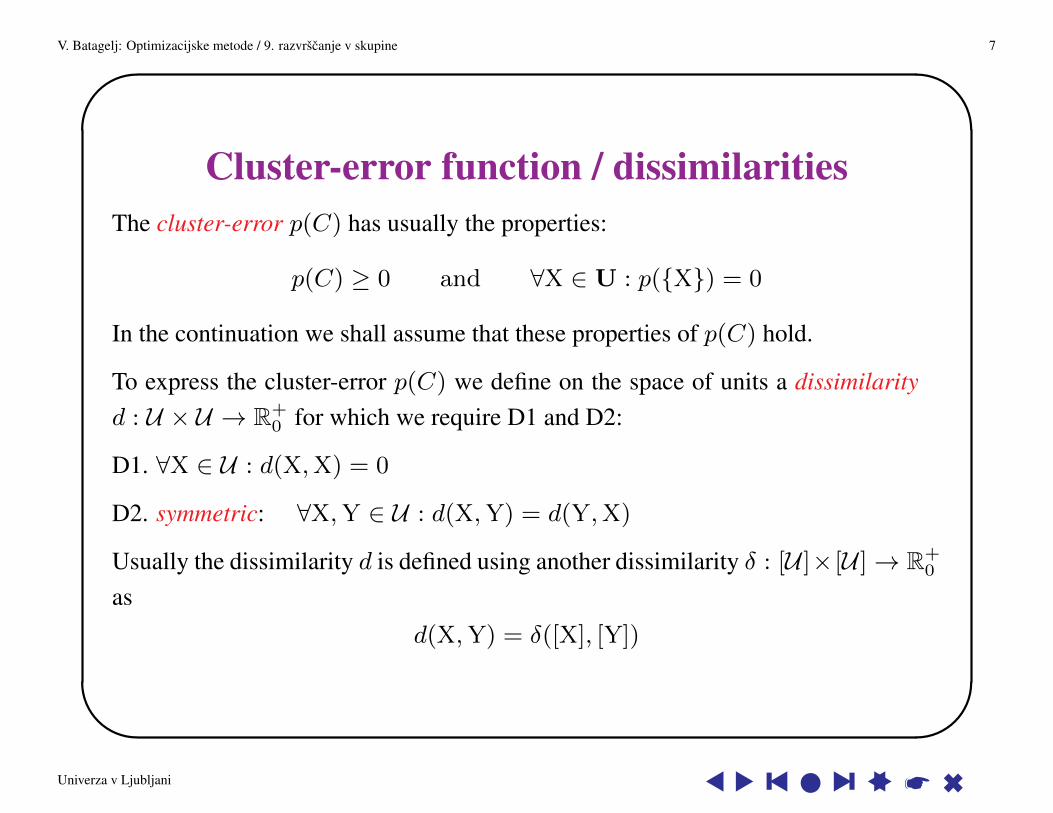
Cluster-error function / dissimilaritiesThe cluster-error p(C) has usually the properties:

p(C) ≥ 0 and ∀X ∈ U : p({X}) = 0

In the continuation we shall assume that these properties of p(C) hold.

To express the cluster-error p(C) we define on the space of units a dissimilarityd : U × U → R+

0 for which we require D1 and D2:

D1. ∀X ∈ U : d(X,X) = 0

D2. symmetric: ∀X,Y ∈ U : d(X,Y) = d(Y,X)

Usually the dissimilarity d is defined using another dissimilarity δ : [U ]× [U ]→ R+0

as

d(X,Y) = δ([X], [Y])



&

$

%

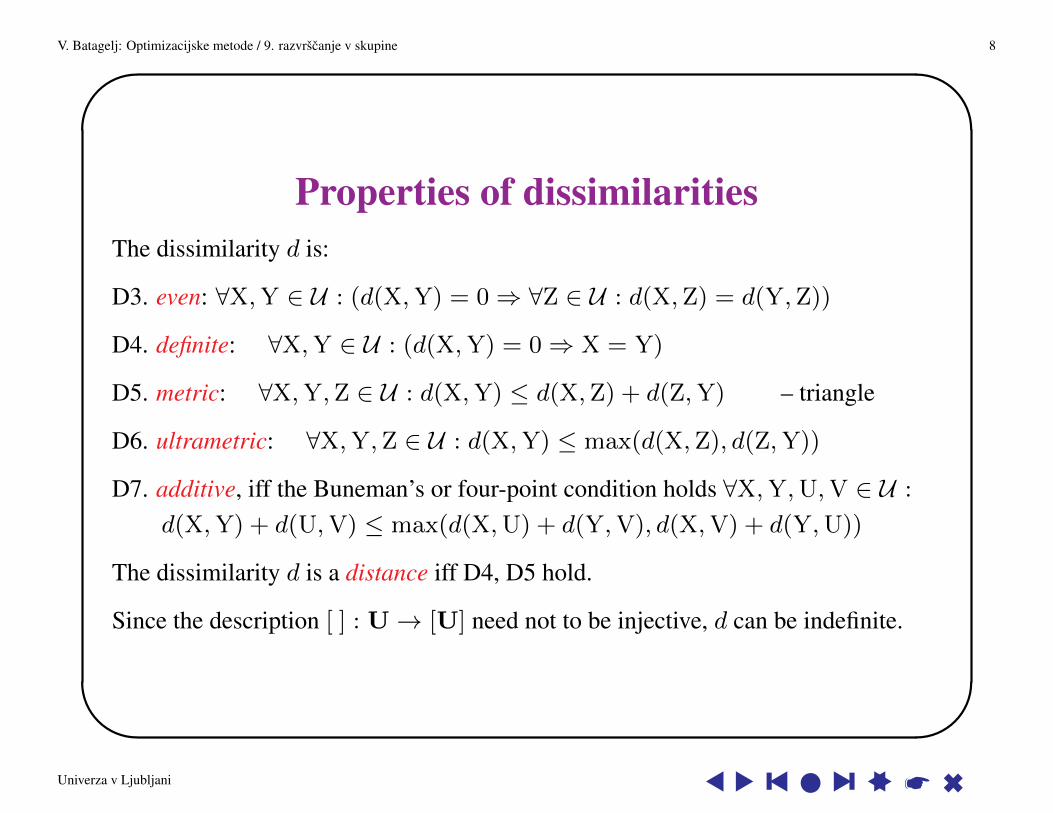
Properties of dissimilaritiesThe dissimilarity d is:

D3. even: ∀X,Y ∈ U : (d(X,Y) = 0⇒ ∀Z ∈ U : d(X,Z) = d(Y,Z))

D4. definite: ∀X,Y ∈ U : (d(X,Y) = 0⇒ X = Y)

D5. metric: ∀X,Y,Z ∈ U : d(X,Y) ≤ d(X,Z) + d(Z,Y) – triangle

D6. ultrametric: ∀X,Y,Z ∈ U : d(X,Y) ≤ max(d(X,Z), d(Z,Y))

D7. additive, iff the Buneman’s or four-point condition holds ∀X,Y,U,V ∈ U :

d(X,Y) + d(U,V) ≤ max(d(X,U) + d(Y,V), d(X,V) + d(Y,U))

The dissimilarity d is a distance iff D4, D5 hold.

Since the description [ ] : U→ [U] need not to be injective, d can be indefinite.



&

$

%

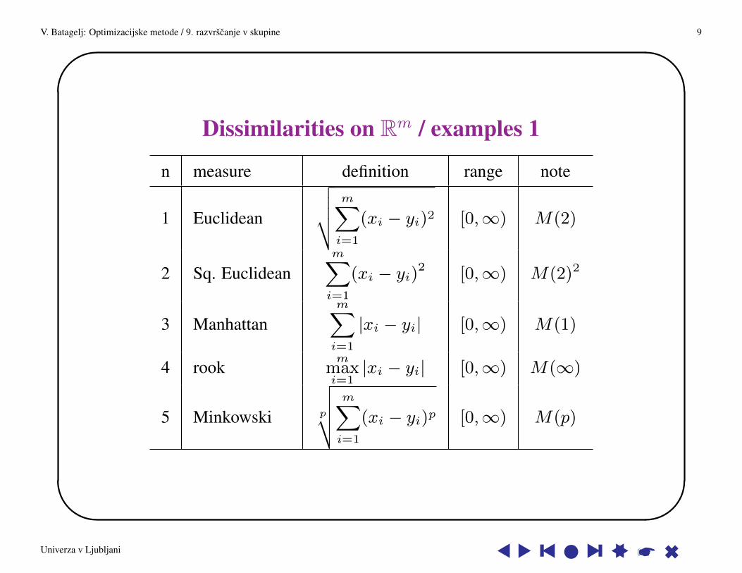
Dissimilarities on Rm / examples 1

n measure definition range note

1 Euclidean

√√√√ m∑i=1

(xi − yi)2 [0,∞) M(2)

2 Sq. Euclideanm∑i=1

(xi − yi)2 [0,∞) M(2)2

3 Manhattanm∑i=1

|xi − yi| [0,∞) M(1)

4 rookm

maxi=1|xi − yi| [0,∞) M(∞)

5 Minkowski p

√√√√ m∑i=1

(xi − yi)p [0,∞) M(p)



&

$

%

Dissimilarities on Rm / examples 2

n measure definition range note

6 Canberram∑i=1

|xi − yi||xi + yi|

[0,∞)

7 Heincke

√√√√ m∑i=1

(|xi − yi||xi + yi|

)2 [0,∞)

8 Self-balancedm∑i=1

|xi − yi|max(xi, yi)

[0,∞)

9 Lance-Williams∑mi=1 |xi − yi|∑mi=1 xi + yi

[0,∞)

10 Correlation c.cov(X,Y )√

var(X)var(Y )[1,−1]



&

$

%

(Dis)similarities on IBm / examplesLet IB = {0, 1}. For X,Y ∈ IBm we define a = XY , b = XY , c = XY ,d = XY . It holds a + b + c + d = m. The counters a, b, c, d are used to defineseveral (dis)similarity measures on binary vectors.

In some cases the definition can yield an indefinite expression 00

. In such cases wecan restrict the use of the measure, or define the values also for indefinite cases. Forexample, we extend the values of Jaccard coefficient such that s4(X,X) = 1. Andfor Kulczynski coefficient, we preserve the relation T = 1

s4− 1 by

s4 =

1 d = m

aa+b+c

otherwises−1

3 = T =

0 a = 0, d = m

∞ a = 0, d < m

b+ca

otherwise

We transform a similarity s from [1, 0] into dissimilarity d on [0, 1] by d = 1− s.

For details see Batagelj, Bren (1995).



&

$

%

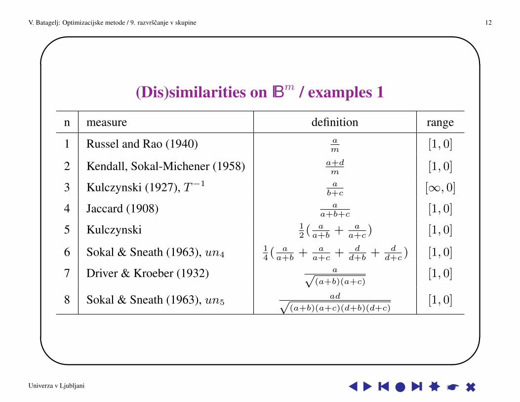
(Dis)similarities on IBm / examples 1

n measure definition range

1 Russel and Rao (1940) am

[1, 0]

2 Kendall, Sokal-Michener (1958) a+dm

[1, 0]

3 Kulczynski (1927), T−1 ab+c

[∞, 0]

4 Jaccard (1908) aa+b+c

[1, 0]

5 Kulczynski 12( aa+b

+ aa+c

) [1, 0]

6 Sokal & Sneath (1963), un414( aa+b

+ aa+c

+ dd+b

+ dd+c

) [1, 0]

7 Driver & Kroeber (1932) a√(a+b)(a+c)

[1, 0]

8 Sokal & Sneath (1963), un5ad√

(a+b)(a+c)(d+b)(d+c)[1, 0]



&

$

%

(Dis)similarities on IBm / examples 2

n measure definition range

9 Q0bcad

[0,∞]

10 Yule (1927), Q ad−bcad+bc

[1,−1]

11 Pearson, φ ad−bc√(a+b)(a+c)(d+b)(d+c)

[1,−1]

12 – bc – 4bcm2 [0, 1]

13 Baroni-Urbani, Buser (1976), S∗∗ a+√ad

a+b+c+√ad

[1, 0]

14 Braun-Blanquet (1932) amax(a+b,a+c)

[1, 0]

15 Simpson (1943) amin(a+b,a+c)

[1, 0]

16 Michael (1920) 4(ad−bc)(a+d)2+(b+c)2

[1,−1]



&

$

%

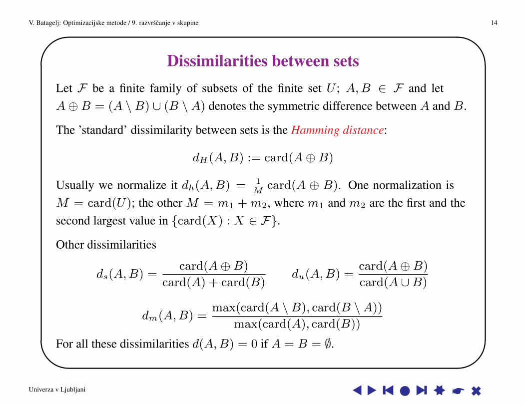
Dissimilarities between setsLet F be a finite family of subsets of the finite set U ; A,B ∈ F and letA⊕B = (A \B) ∪ (B \A) denotes the symmetric difference between A and B.

The ’standard’ dissimilarity between sets is the Hamming distance:

dH(A,B) := card(A⊕B)

Usually we normalize it dh(A,B) = 1M

card(A ⊕ B). One normalization isM = card(U); the other M = m1 + m2, where m1 and m2 are the first and thesecond largest value in {card(X) : X ∈ F}.

Other dissimilarities

ds(A,B) =card(A⊕B)

card(A) + card(B)du(A,B) =

card(A⊕B)

card(A ∪B)

dm(A,B) =max(card(A \B), card(B \A))

max(card(A), card(B))

For all these dissimilarities d(A,B) = 0 if A = B = ∅.



&

$

%

Problems with dissimilaritiesWhat to do in the case of mixed units (with variables measured in different types ofscales)?

• conversion to a common scale

• compute the dissimilarities on homogeneous parts and combine them (Gower’sdissimilarity)

Fairness of dissimilarity – all variables contribute equally. Approaches: use ofnormalized variables, analysis of dependencies among variables.



&

$

%

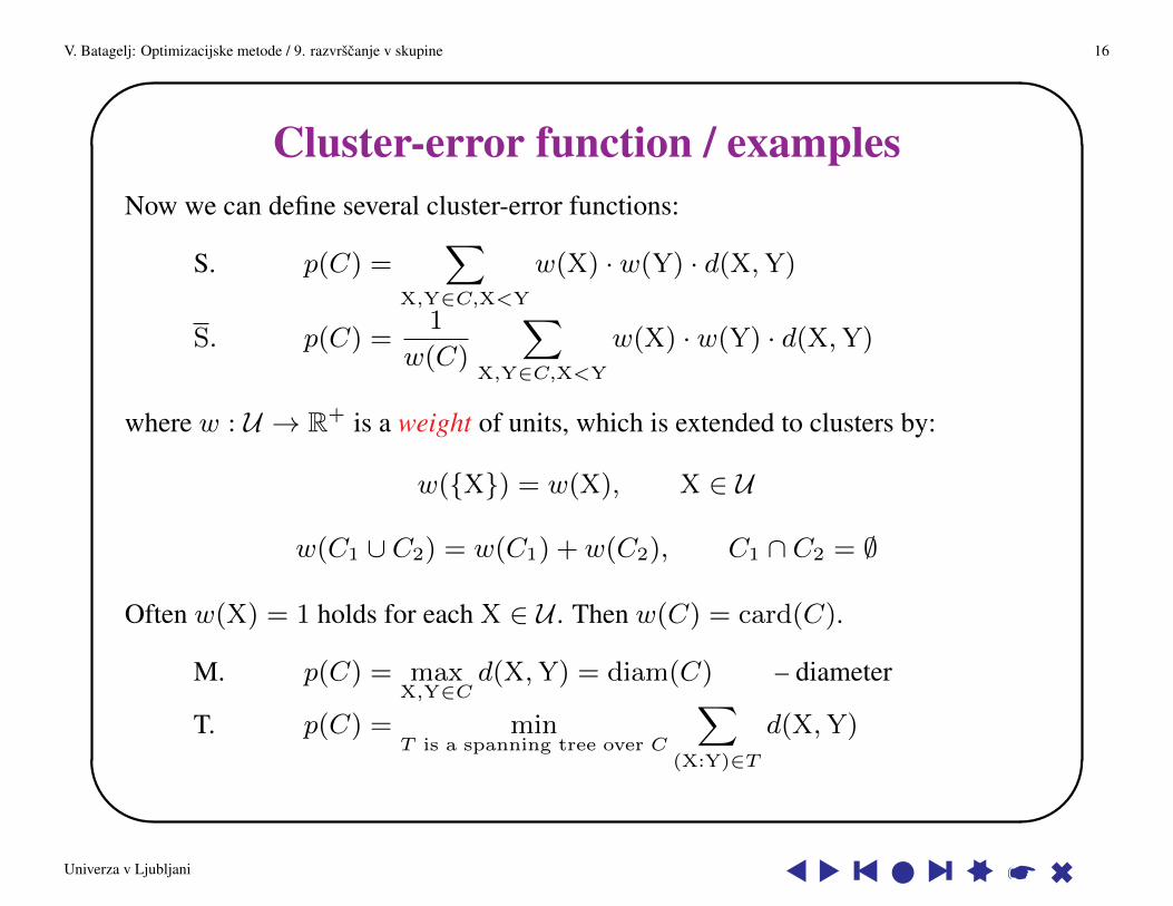
Cluster-error function / examplesNow we can define several cluster-error functions:

S. p(C) =∑

X,Y∈C,X<Y

w(X) · w(Y) · d(X,Y)

S. p(C) =1

w(C)

∑X,Y∈C,X<Y

w(X) · w(Y) · d(X,Y)

where w : U → R+ is a weight of units, which is extended to clusters by:

w({X}) = w(X), X ∈ U

w(C1 ∪ C2) = w(C1) + w(C2), C1 ∩ C2 = ∅

Often w(X) = 1 holds for each X ∈ U . Then w(C) = card(C).

M. p(C) = maxX,Y∈C

d(X,Y) = diam(C) – diameter

T. p(C) = minT is a spanning tree over C

∑(X:Y)∈T

d(X,Y)



&

$

%

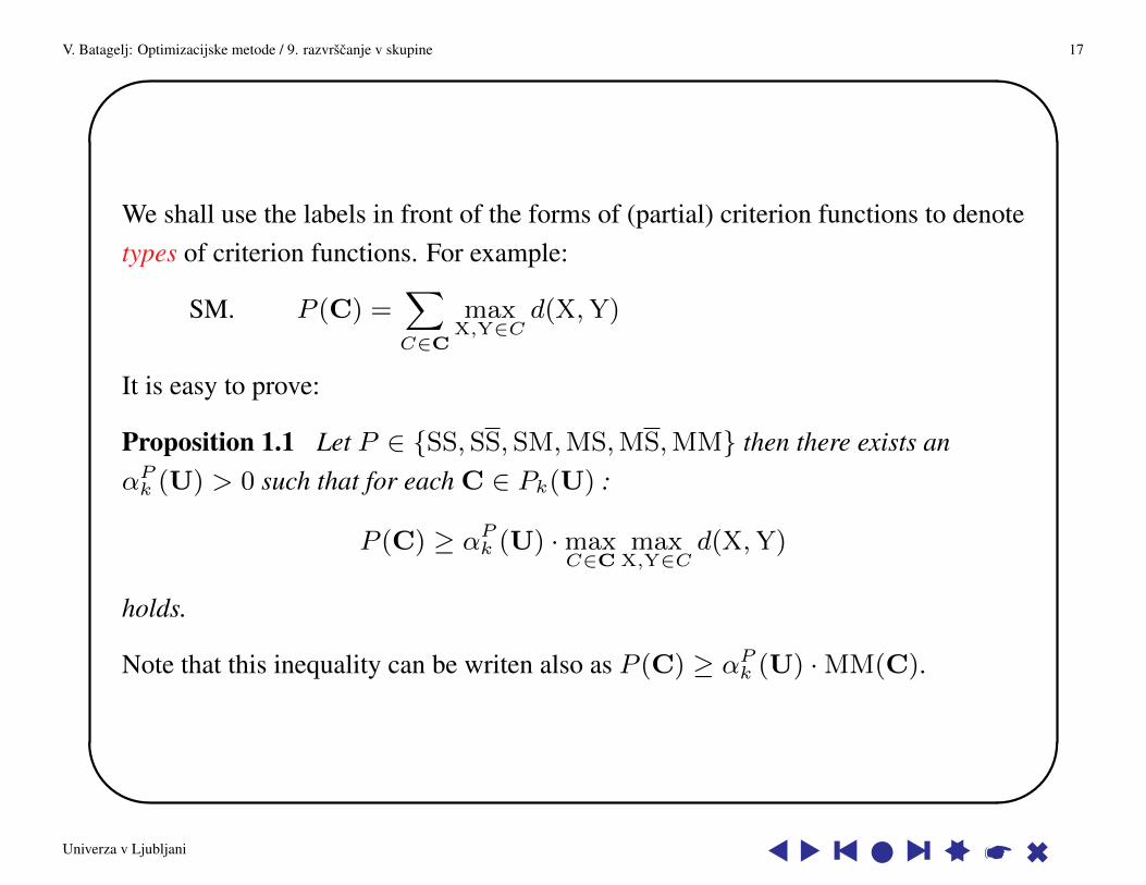
We shall use the labels in front of the forms of (partial) criterion functions to denotetypes of criterion functions. For example:

SM. P (C) =∑C∈C

maxX,Y∈C

d(X,Y)

It is easy to prove:

Proposition 1.1 Let P ∈ {SS, SS, SM,MS,MS,MM} then there exists anαPk (U) > 0 such that for each C ∈ Pk(U) :

P (C) ≥ αPk (U) ·maxC∈C

maxX,Y∈C

d(X,Y)

holds.

Note that this inequality can be writen also as P (C) ≥ αPk (U) ·MM(C).



&

$

%

Sensitive criterion functionsThe criterion function P (C), based on the dissimilarity d, is sensitive iff for eachfeasible clustering C it holds

P (C) = 0⇐⇒ ∀C ∈ C ∀X,Y ∈ C : d(X,Y) = 0

and is α-sensitive iff there exists an αPk (U) > 0 such that for each C ∈ Pk(U) :

P (C) ≥ αPk (U) ·MM(C)

Proposition 1.2 Every α-sensitive criterion function is also sensitive.

The proposition 1.1 can be reexpressed as:

Proposition 1.3 The criterion functions SS, SS, SM,MS,MS,MM are α-sensitive.



&

$

%

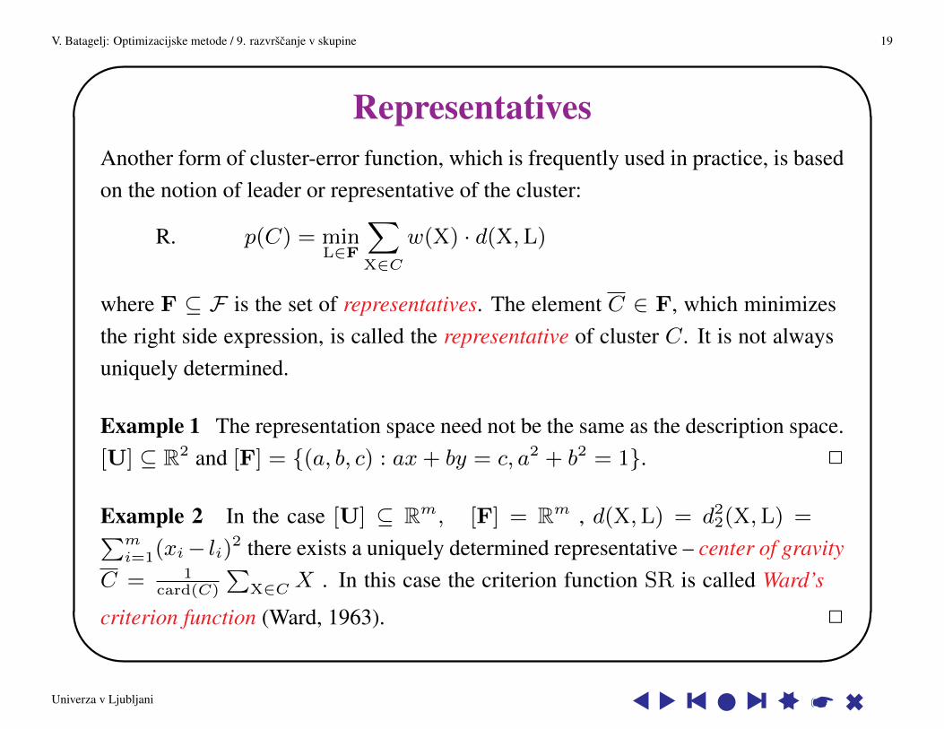
RepresentativesAnother form of cluster-error function, which is frequently used in practice, is basedon the notion of leader or representative of the cluster:

R. p(C) = minL∈F

∑X∈C

w(X) · d(X,L)

where F ⊆ F is the set of representatives. The element C ∈ F, which minimizesthe right side expression, is called the representative of cluster C. It is not alwaysuniquely determined.

Example 1 The representation space need not be the same as the description space.[U] ⊆ R2 and [F] = {(a, b, c) : ax+ by = c, a2 + b2 = 1}. 2

Example 2 In the case [U] ⊆ Rm, [F] = Rm , d(X,L) = d22(X,L) =∑m

i=1(xi− li)2 there exists a uniquely determined representative – center of gravityC = 1

card(C)

∑X∈C X . In this case the criterion function SR is called Ward’s

criterion function (Ward, 1963). 2



&

$

%

The generalized Ward’s criterion functionTo obtain the generalized Ward’s clustering problem we, relying on the equality

p(C) =∑X∈C

d22(X,C) =

1

2 card(C)

∑X,Y ∈C

d22(X,Y )

replace the expression for p(C) with

p(C) =1

2w(C)

∑X,Y ∈C

w(X) · w(Y ) · d(X,Y ) = S(C)

Note that d can be any dissimilarity on U .

From the definition we can easily derive the following equality: If Cu ∩ Cv = ∅then

w(Cu∪Cv)·p(Cu∪Cv) = w(Cu)·p(Cu)+w(Cv)·p(Cv)+∑

X∈Cu,Y ∈Cv

w(X)·w(Y )·d(X,Y )

In Batagelj (1988) it is also shown how to replace C by a generalized, possiblyimaginary (with descriptions not neccessary in the same set as U), central elementin the way to preserve the properties characteristic for Ward’s clustering problem.



&

$

%

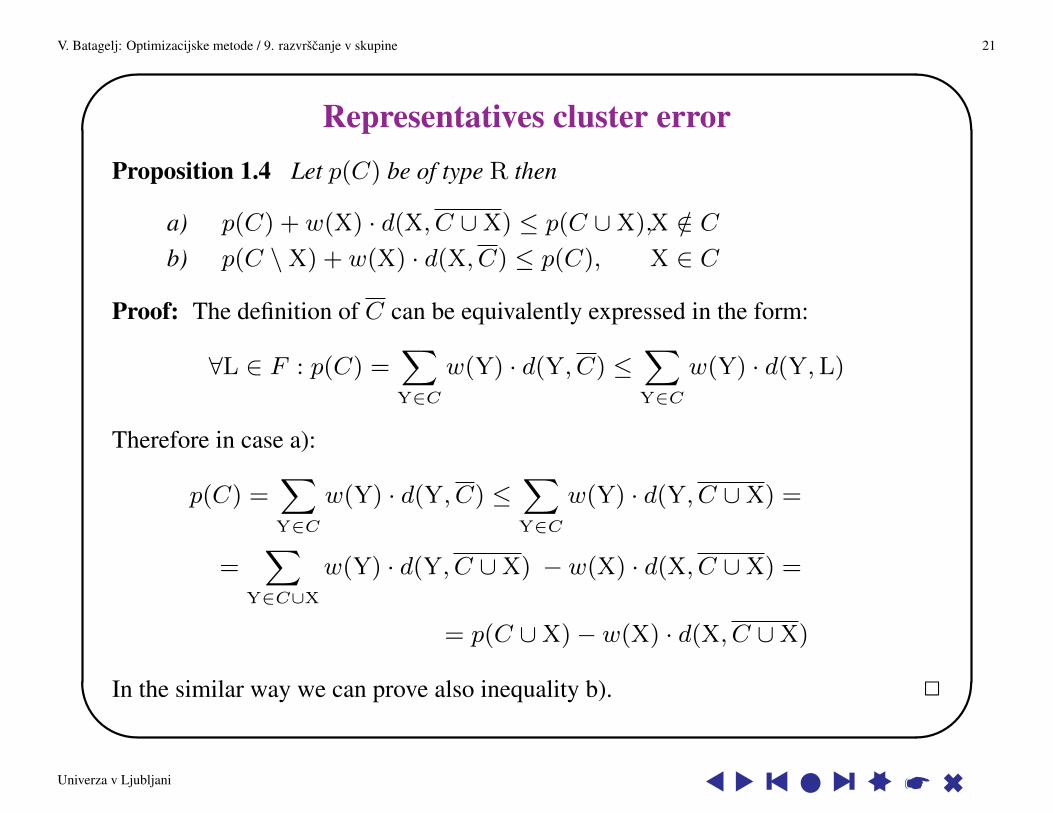
Representatives cluster errorProposition 1.4 Let p(C) be of type R then

a) p(C) + w(X) · d(X, C ∪X) ≤ p(C ∪X),X /∈ Cb) p(C \X) + w(X) · d(X, C) ≤ p(C), X ∈ C

Proof: The definition of C can be equivalently expressed in the form:

∀L ∈ F : p(C) =∑Y∈C

w(Y) · d(Y, C) ≤∑Y∈C

w(Y) · d(Y,L)

Therefore in case a):

p(C) =∑Y∈C

w(Y) · d(Y, C) ≤∑Y∈C

w(Y) · d(Y, C ∪X) =

=∑

Y∈C∪X

w(Y) · d(Y, C ∪X) − w(X) · d(X, C ∪X) =

= p(C ∪X)− w(X) · d(X, C ∪X)

In the similar way we can prove also inequality b). 2



&

$

%

Other criterion functionsSeveral other types of criterion functions were proposed in the literature. A veryimportant class among them are the ”statisticalcriterion functions based on theassumption that the units are sampled from a mixture of multivariate normaldistributions (Marriott, 1982) .

General criterion functionNot all clustering problems can be expressed by a simple criterion function. In someapplications a general criterion function of the form

P (C) =⊕

(C1,C2)∈C×C

q(C1, C2), q(C1, C2) ≥ 0

is needed. We shall use it in blockmodeling.

Multicriteria clusteringIn some problems several criterion functions can be defined (Φ, P1, P2, . . . , Ps).See Ferligoj, Batagelj (1994).



&

$

%

Example: problem of partitioning of a generation of pupilsinto a given number of classes

so that the classes will consist of (almost) the same number of pupils and that theywill have a structure as similar as possible. An appropriate criterion function is

P (C) = max{C1,C2}∈C×C

card(C1)≥card(C2)

minf:C1→C2f is surjective

maxX∈C1

d(X, f(X))

where d(X,Y) is a measure of dissimilarity between pupils X and Y.



&

$

%

Example: RegionalizationThe motivation comes from regionalization problem: partition given set of territorialunits into k connected subgroups of similar units – regions.

Suppose that besides the descriptions of units [U] they are related also by a binaryrelation R ⊆ U×U.

In such a case we have an additional requirement – relational constraint onclusterings to be feasible. The set of feasible clusterings can be defined as:

Φ(R) = {C ∈ P (U) : each cluster C ∈ C is a subgraph (C,R ∩ C × C) in thegraph (U, R) with the required type of connectedness}

If R is nonsymmetric we can define different types of sets of feasible clusterings forthe same relation (Ferligoj and Batagelj, 1983).



&

$

%

Complexity of the clustering problemBecause the set of feasible clusterings Φ is finite the clustering problem (Φ, P )

can be solved by the brute force approach inspecting all feasible clusterings.Unfortunately, the number of feasible clusterings grows very quickly with n. Forexample

card(Pk) = S(n, k) =1

k!

k−1∑i=0

(−1)i(k

i

)(k − i)n, 0 < k ≤ n

where S(n, k) is a Stirling number of the second kind. And to get an impression:

S(20, 8) = 15170932662679

S(30, 11) = 215047101560666876619690

S(n, 2) = 2n−1 − 1

For this reason the brute force algorithm is only of theoretical interest.

We shall assume that the reader is familiar with the basic notions of the theory ofcomplexity of algorithms (Garey and Johnson, 1979) .



&

$

%

Complexity resultsAlthough there are some polynomial types of clustering problems, for example(P2,MM) and (Pk, ST), it seems that they are mainly NP-hard.

Brucker (1978) showed that ( ∝ denotes the polynomial reducibility of problems) :

Theorem 1.5 Let the criterion function

P (C) =⊕C∈C

p(C)

be α-sensitive, then for each problem (Pk(U), P ) there exists a problem(Pk+1(U′), P ), such that (Pk(U), P ) ∝ (Pk+1(U′), P ).



&

$

%

Proof: Select a value P ∗ such that P ∗ > maxC∈Pk(U) P (C), extend, U′ = U ∪ {X•},the set of units with a new unit X•, and define the dissimilarities between it and the ’old’ unitssuch that d(X,X•) > P ∗/α′, for X ∈ U and α′ = αPk+1(U

′). We get a new clusteringproblem (Pk+1(U

′), P ).

Consider a clustering C′ ∈ Pk+1(U′). There are two possibilities:

a. X• forms its own cluster C′ = C ∪ {{X•}}, C ∈ Pk(U). Then

P (C′) = P (C)⊕ p({X•}) = P (C) ≤ maxC∈Pk(U)

P (C) < P ∗

b. X• belongs to a cluster C• with card(C•) ≥ 2. Then

P (C′) ≥ α′ · maxC∈C′

maxX,Y∈C

d(X,Y) ≥ α′ · maxX,Y∈C•

d(X,Y) =

= α′ · maxX∈C•\{X•}

d(X,X•) > P ∗

We see that all optimal solutions of the problem (Pk+1(U′), P ) have the form a. Since in

this case P (C′) = P (C)

C′ ∈ Min(Pk+1(U′), P )⇔ C ∈ Min(Pk(U), P )

2



&

$

%

Complexity results 1Theorem 1.6 Let the criterion function P be sensitive then

3− COLOR ∝ (P3, P )

Proof: Let G = (V,E) be a simple undirected graph. We assign to it a clusteringproblem (P3(V ), P ) as follows. We define a dissimilarity d (on which P is based)by

d(u, v) =

1 (u : v) ∈ E

0 (u : v) /∈ E

Since P is sensitive it holds: the graph G is 3-colorable iff min(P3(V ), P ) = 0.Let C = {C1, C2, C3} then P (C) = 0 iff c :

V → {1, 2, 3} : (c(v) = i ⇔ v ∈ Ci) is avertex coloring.

2



&

$

%

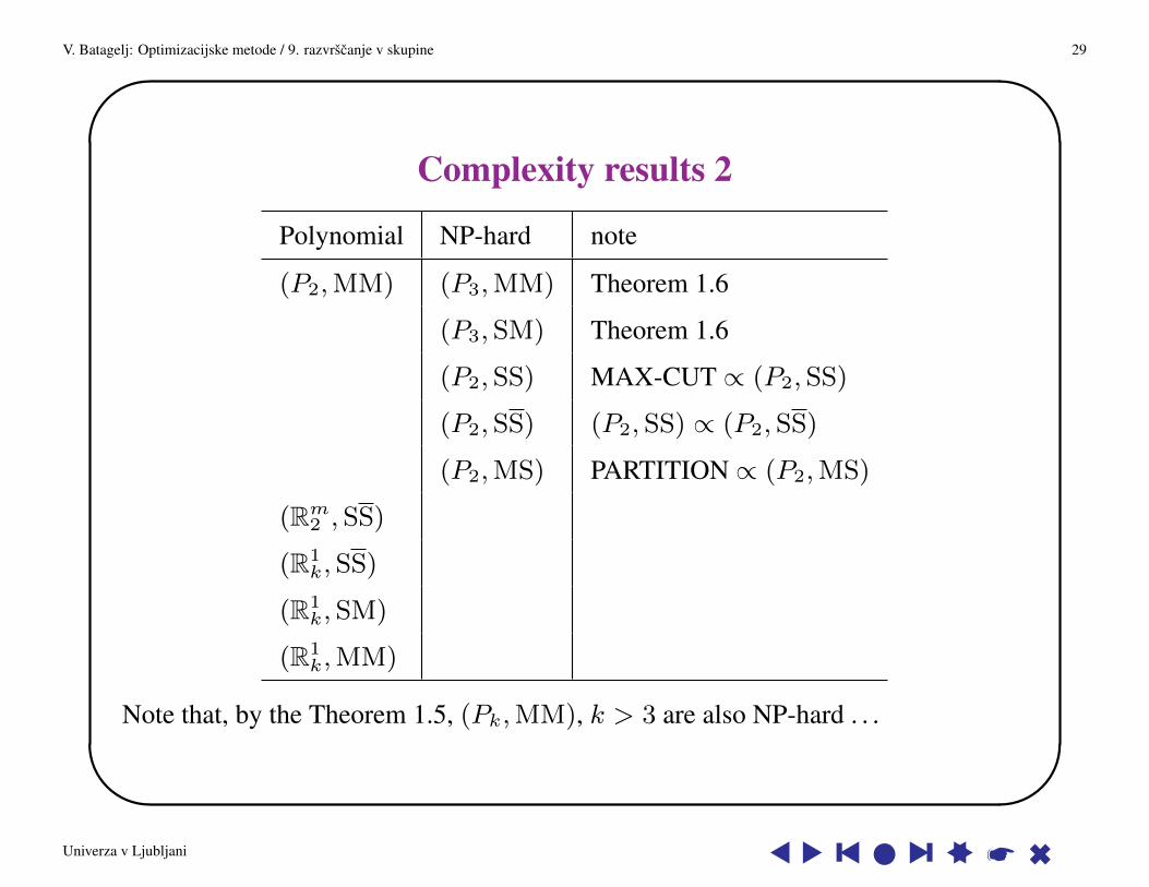
Complexity results 2

Polynomial NP-hard note

(P2,MM) (P3,MM) Theorem 1.6

(P3,SM) Theorem 1.6

(P2,SS) MAX-CUT ∝ (P2,SS)

(P2,SS) (P2, SS) ∝ (P2, SS)

(P2,MS) PARTITION ∝ (P2,MS)

(Rm2 , SS)

(R1k, SS)

(R1k, SM)

(R1k,MM)

Note that, by the Theorem 1.5, (Pk,MM), k > 3 are also NP-hard . . .



&

$

%

ConsequencesFrom these results it follows (it is believed) that no efficient (polynomial) exactalgorithm exists for solving the clustering problem.

Therefore the procedures should be used which give ”good”results, but notnecessarily the best, in a reasonable time.

The most important types of these procedures are:

• local optimization

• hierarchical (agglomerative, divisive and adding)

• leaders and the dynamic clusters method

• graph theory methods



&

$

%

Approaches to Clustering• local optimization

• dynamic programming

• hierarchical methods; agglomerative methods; Lance-Williams formula;dendrogram; inversions; adding methods

• leaders and the dynamic clusters method

• graph theory (next, 3. lecture);



&

$

%

Local optimizationOften for a given optimization problem (Φ, P ) there exist rules which relate to eachelement of the set Φ some elements of Φ. We call them local transformations.

The elements which can be obtained from a given element are called neighbors –local transformations determine the neighborhood relation S ⊆ Φ×Φ in the set Φ.The neighborhood of element X ∈ Φ is called the set S(X) = {Y : XSY} .The element X ∈ Φ is a local minimum for the neighborhood structure (Φ, S) iff

∀Y ∈ S(X) : P (X) ≤ P (Y)

In the following we shall assume that S is reflexive, ∀X ∈ Φ : XSX.



&

$

%

Local optimizationThey are the basis of the local optimization procedure

select X0; X := X0;while ∃Y ∈ S(X) : P (Y) < P (X) do X := Y;

which starting in an element of X0 ∈ Φ repeats moving to an element determinedby local transformation which has better value of the criterion function until no suchelement exists.



&

$

%

Clustering neigborhoodsUsually the neighborhood relation in local optimization clustering procedures overPk(U) is determined by the following two transformations:

• transition: clustering C′ is obtained from C by moving a unit from one clusterto another

C′ = (C \ {Cu, Cv}) ∪ {Cu \ {Xs}, Cv ∪ {Xs}}

• transposition: clustering C′ is obtained from C by interchanging two unitsfrom different clusters

C′ = (C \ {Cu, Cv}) ∪ {(Cu \ {Xp}) ∪ {Xq}, (Cv \ {Xq}) ∪ {Xp}}

The transpositions preserve the number of units in clusters.



&

$

%

HintsTwo basic implementation approaches are usually used: stored data approach andstored dissimilarity matrix approach.

If the constraints are not too stringent, the relocation method can be applied directlyon Φ; otherwise, we can transform using penalty function method the problem to anequivalent nonconstrained problem (Pk, Q) with Q(C) = P (C) + αK(C) whereα > 0 is a large constant and K(C) = 0, for C ∈ Φ, and K(C) > 0 otherwise.

There exist several improvements of the basic relocation algorithm: simulatedannealing, tabu search, . . . (Aarts and Lenstra, 1997).

The initial clustering C0 can be given; most often we generate it randomly.Let c[s] = u⇔ Xs ∈ Cu. Fill the vector c with the desired number of units in eachcluster and shuffle it:

for p := n downto 2 do begin q := random(1, p); swap(c[p], c[q]) end;



&

$

%

Quick scanning of neighborsTesting P (C′) < P (C) is equivalent to P (C)− P (C′) > 0.For the S criterion function

∆P (C,C′) = P (C)− P (C′) = p(Cu) + p(Cv)− p(C′u)− p(C′v)

Additional simplifications can be done considering relations between Cu and C′u,and between Cv and C′v .

Let us illustrate this on the generalized Ward’s method. For this purpose it is usefulto introduce the quantity

a(Cu, Cv) =∑

X∈Cu,Y∈Cv

w(X) · w(Y) · d(X,Y)

Using the quantity a(Cu, Cv) we can express p(C) in the form p(C) = a(C,C)2w(C)

and the equality mentioned in the introduction of the generalized Ward clusteringproblem: if Cu ∩ Cv = ∅ then

w(Cu ∪ Cv) · p(Cu ∪ Cv) = w(Cu) · p(Cu) + w(Cv) · p(Cv) + a(Cu, Cv)



&

$

%

∆ for the generalized Ward’s methodLet us analyze the transition of a unit Xs from cluster Cu to cluster Cv:We have C′u = Cu \ {Xs} , C′v = Cv ∪ {Xs} ,

w(Cu)·p(Cu) = w(C′u)·p(C′u)+a(Xs, C′u) = (w(Cu)−w(Xs))·p(C′u)+a(Xs, C

′u)

andw(C′v) · p(C′v) = w(Cv) · p(Cv) + a(Xs, Cv)

From d(Xs,Xs) = 0 it follows a(Xs, Cu) = a(Xs, C′u). Therefore

p(C′u) =w(Cu) · p(Cu)− a(Xs, Cu)

w(Cu)− w(Xs)p(C′v) =

w(Cv) · p(Cv) + a(Xs, Cv)

w(Cv) + w(Xs)

and finally

∆P (C,C′) = p(Cu) + p(Cv)− p(C′u)− p(C′v) =

=w(Xs) · p(Cv)− a(Xs, Cv)

w(Cv) + w(Xs)− w(Xs) · p(Cu)− a(Xs, Cu)

w(Cu)− w(Xs)

In the case when d is the squared Euclidean distance it is possible to derive also

expression for corrections of centers (Spath, 1977).



&

$

%

Dynamic programmingSuppose that Min(Φk, P ) 6= ∅, k = 1, 2, . . .. Denoting P ∗(U, k) =P (C∗k(U)) we can derive the generalized Jensen equality (Batagelj,Korenjak and Klavzar, 1994):

P ∗(U, k) =

p(U) {U} ∈ Φ1

min∅⊂C⊂U

∃C∈Φk−1(U\C):C∪{C}∈Φk(U)

(P ∗(U \ C, k − 1)⊕ p(C)) k > 1

This is a dynamic programming (Bellman) equation which, for some specialconstrained problems, that keep the size of Φk small, allows us to solve theclustering problem by the adapted Fisher’s algorithm.



&

$

%

Hierarchical methodsThe set of feasible clusterings Φ determines the feasibility predicate Φ(C) ≡ C ∈Φ defined onP(P(U)\{∅}); and conversely Φ ≡ {C ∈ P(P(U)\{∅}) : Φ(C)}.

In the set Φ the relation of clustering inclusion v can be introduced by

C1 v C2 ≡ ∀C1 ∈ C1, C2 ∈ C2 : C1 ∩ C2 ∈ {∅, C1}

we say also that the clustering C1 is a refinement of the clustering C2.

It is well known that (P (U),v) is a partially ordered set (even more, semimodularlattice). Because any subset of partially ordered set is also partially ordered, wehave: Let Φ ⊆ P (U) then (Φ,v) is a partially ordered set.

The clustering inclusion determines two related relations (on Φ):

C1 < C2 ≡ C1 v C2 ∧C1 6= C2 – strict inclusion, and

C1 <· C2 ≡ C1 < C2 ∧ ¬∃C ∈ Φ : (C1 < C ∧C < C2) – predecessor.



&

$

%

Conditions on the structure of the set of feasible clusteringsWe shall assume that the set of feasible clusterings Φ ⊆ P (U) satisfies thefollowing conditions:

F1. O ≡ {{X} : X ∈ U} ∈ Φ

F2. The feasibility predicate Φ is local – it has the form Φ(C) =∧C∈C ϕ(C)

where ϕ(C) is a predicate defined on P(U) \ {∅} (clusters).

The intuitive meaning of ϕ(C) is: ϕ(C) ≡ the cluster C is ’good’. Thereforethe locality condition can be read: a ’good’ clustering C ∈ Φ consists of ’good’clusters.

F3. The predicate Φ has the property of binary heredity with respect to thefusibility predicate ψ(C1, C2), i.e.,

C1 ∩ C2 = ∅ ∧ ϕ(C1) ∧ ϕ(C2) ∧ ψ(C1, C2)⇒ ϕ(C1 ∪ C2)

This condition means: in a ’good’ clustering, a fusion of two ’fusible’ clustersproduces a ’good’ clustering.



&

$

%

. . . conditions

F4. The predicate ψ is compatible with clustering inclusion v, i.e.,

∀C1,C2 ∈ Φ : (C1 < C2 ∧C1 \C2 = {C1, C2} ⇒ ψ(C1, C2) ∨ ψ(C2, C1))

F5. The interpolation property holds in Φ, i.e., ∀C1,C2 ∈ Φ :

(C1 < C2 ∧ card(C1) > card(C2) + 1⇒ ∃C ∈ Φ : (C1 < C ∧C < C2))

These conditions provide a framework in which the hierarchical methods can beapplied also for constrained clustering problems Φk(U) ⊂ Pk(U).

In the ordinary problem both predicates ϕ(C) and ψ(Cp, Cq) are always true – allconditions F1-F5 are satisfied.



&

$

%

Criterion functions compatible with a dissimilaritybetween clusters

We shall call a dissimilarity between clusters a function D : (C1, C2)→ R+0 which

is symmetric, i.e., D(C1, C2) = D(C2, C1).

Let (R+0 ,⊕, 0,≤) be an ordered abelian monoid. Then the criterion function

P (C) =⊕

C∈C p(C), ∀X ∈ U : p({X}) = 0 is compatible with dissimilarity Dover Φ iff for all C ⊆ U holds:

ϕ(C) ∧ card(C) > 1⇒ p(C) = min(C1,C2)∈Ψ(C)

(p(C1)⊕ p(C2)⊕D(C1, C2))

Theorem 1.7 A S criterion function is compatible with dissimilarity D defined by

D(Cp, Cq) = p(Cp ∪ Cq)− p(Cp)− p(Cq)

In this case, let C′ = C \ {Cp, Cq} ∪ {Cp ∪ Cq}, Cp, Cq ∈ C, then

P (C′)− P (C) = D(Cp, Cq)



&

$

%

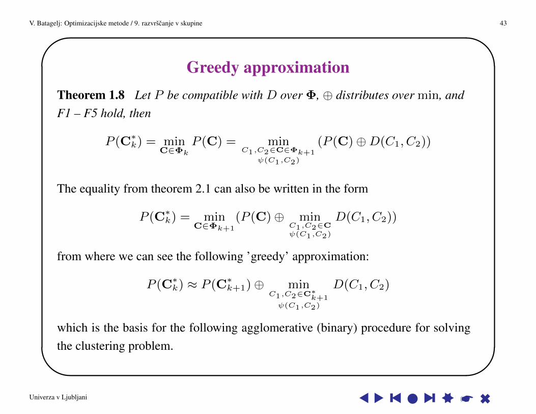
Greedy approximationTheorem 1.8 Let P be compatible with D over Φ, ⊕ distributes over min, andF1 – F5 hold, then

P (C∗k) = minC∈Φk

P (C) = minC1,C2∈C∈Φk+1

ψ(C1,C2)

(P (C)⊕D(C1, C2))

The equality from theorem 2.1 can also be written in the form

P (C∗k) = minC∈Φk+1

(P (C)⊕ minC1,C2∈Cψ(C1,C2)

D(C1, C2))

from where we can see the following ’greedy’ approximation:

P (C∗k) ≈ P (C∗k+1)⊕ minC1,C2∈C∗

k+1ψ(C1,C2)

D(C1, C2)

which is the basis for the following agglomerative (binary) procedure for solvingthe clustering problem.



&

$

%

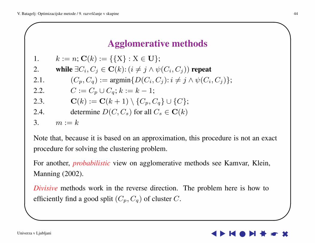
Agglomerative methods1. k := n; C(k) := {{X} : X ∈ U};2. while ∃Ci, Cj ∈ C(k): (i 6= j ∧ ψ(Ci, Cj)) repeat2.1. (Cp, Cq) := argmin{D(Ci, Cj): i 6= j ∧ ψ(Ci, Cj)};2.2. C := Cp ∪ Cq; k := k − 1;2.3. C(k) := C(k + 1) \ {Cp, Cq} ∪ {C};2.4. determine D(C,Cs) for all Cs ∈ C(k)

3. m := k

Note that, because it is based on an approximation, this procedure is not an exactprocedure for solving the clustering problem.

For another, probabilistic view on agglomerative methods see Kamvar, Klein,Manning (2002).

Divisive methods work in the reverse direction. The problem here is how toefficiently find a good split (Cp, Cq) of cluster C.



&

$

%

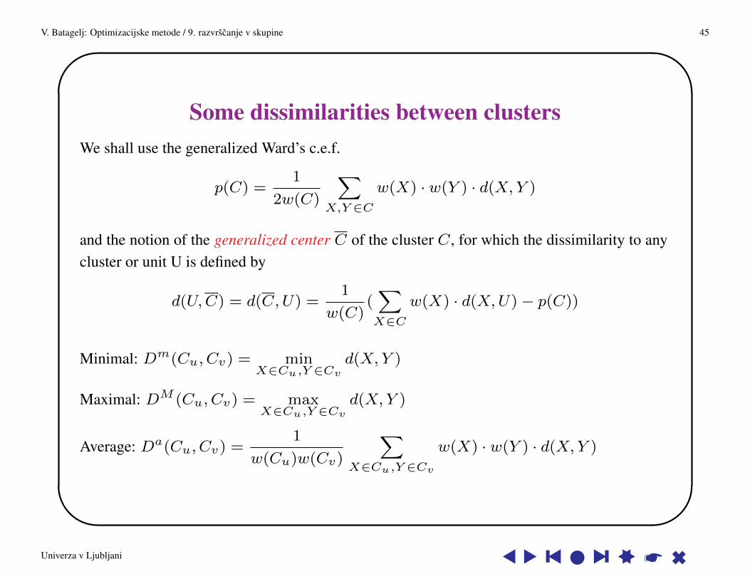
Some dissimilarities between clustersWe shall use the generalized Ward’s c.e.f.

p(C) =1

2w(C)

∑X,Y ∈C

w(X) · w(Y ) · d(X,Y )

and the notion of the generalized center C of the cluster C, for which the dissimilarity to anycluster or unit U is defined by

d(U,C) = d(C,U) =1

w(C)(∑X∈C

w(X) · d(X,U)− p(C))

Minimal: Dm(Cu, Cv) = minX∈Cu,Y ∈Cv

d(X,Y )

Maximal: DM (Cu, Cv) = maxX∈Cu,Y ∈Cv

d(X,Y )

Average: Da(Cu, Cv) =1

w(Cu)w(Cv)

∑X∈Cu,Y ∈Cv

w(X) · w(Y ) · d(X,Y )



&

$

%

. . . some dissimilaritiesGower-Bock: DG(Cu, Cv) = d(Cu, Cv) = Da(Cu, Cv)−

p(Cu)

w(Cu)−p(Cv)

w(Cv)

Ward: DW (Cu, Cv) =w(Cu)w(Cv)

w(Cu ∪ Cv)DG(Cu, Cv)

Inertia: DI(Cu, Cv) = p(Cu ∪ Cv)

Variance: DV (Cu, Cv) = var(Cu ∪ Cv) =p(Cu ∪ Cv)w(Cu ∪ Cv)

Weighted increase of variance:

Dv(Cu, Cv) = var(Cu∪Cv)−w(Cu) · var(Cu) + w(Cv) · var(Cv)

w(Cu ∪ Cv)=DW (Cu, Cv)

w(Cu ∪ Cv)

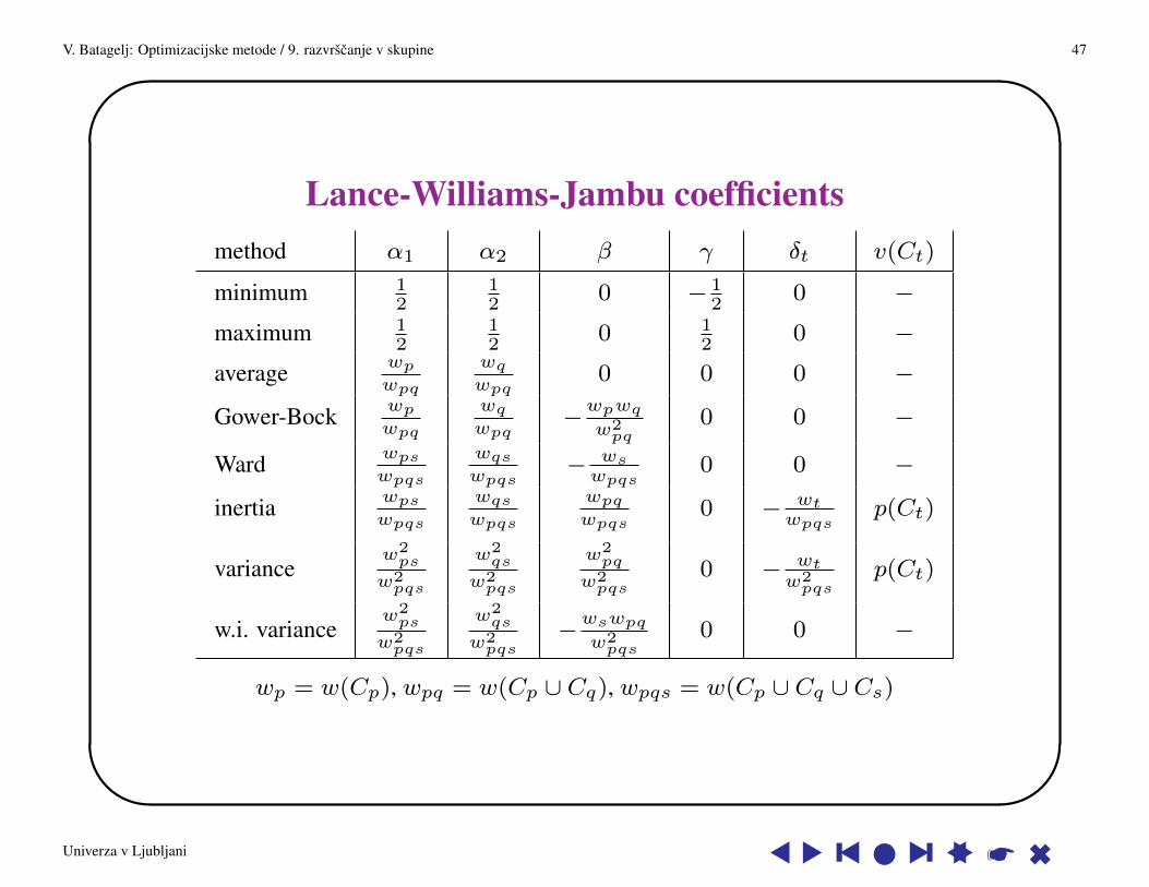
For all of them Lance-Williams-Jambu formula holds:

D(Cp ∪ Cq , Cs) = α1D(Cp, Cs) + α2D(Cq , Cs) + βD(Cp, Cq) +

+γ|D(Cp, Cs)−D(Cq , Cs)|+ δ1v(Cp) + δ2v(Cq) + δ3v(Cs)



&

$

%

Lance-Williams-Jambu coefficientsmethod α1 α2 β γ δt v(Ct)

minimum 12

12

0 − 12

0 −maximum 1

212

0 12

0 −average wp

wpq

wqwpq

0 0 0 −

Gower-Bock wpwpq

wqwpq

−wpwqw2pq

0 0 −

Ward wpswpqs

wqswpqs

− wswpqs

0 0 −

inertia wpswpqs

wqswpqs

wpqwpqs

0 − wtwpqs

p(Ct)

variancew2ps

w2pqs

w2qs

w2pqs

w2pq

w2pqs

0 − wtw2pqs

p(Ct)

w.i. variancew2ps

w2pqs

w2qs

w2pqs

−wswpqw2pqs

0 0 −

wp = w(Cp), wpq = w(Cp ∪ Cq), wpqs = w(Cp ∪ Cq ∪ Cs)



&

$

%

HierarchiesThe agglomerative clustering procedure produces a series of feasible clusterings C(n),C(n− 1), . . . , C(m) with C(m) ∈ MaxΦ (maximal elements for v).

Their union T =⋃nk=m C(k) is called a hierarchy and has the property

∀Cp, Cq ∈ T : Cp ∩ Cq ∈ {∅, Cp, Cq}

The set inclusion ⊆ is a tree or hierarchical order on T . The hierarchy T is complete iffU ∈ T .

For W ⊆ U we define the smallest cluster CT (W ) from T containing W as:c1. W ⊆ CT (W )

c2. ∀C ∈ T : (W ⊆ C ⇒ CT (W ) ⊆ C)

CT is a closure on T with a special property

Z /∈ CT ({X,Y})⇒ CT ({X,Y}) ⊂ CT ({X,Y,Z}) = CT ({X,Z}) = CT ({Y,Z})



&

$

%

Level functionsA mapping h : T → R+

0 is a level function on T iffl1. ∀X ∈ U : h({X}) = 0

l2. Cp ⊆ Cq ⇒ h(Cp) ≤ h(Cq)A simple example of level function is h(C) = card(C)− 1.

Every hierarchy / level function determines an ultrametric dissimilarity on U

δ(X,Y) = h(CT ({X,Y}))

The converse is also true (see Dieudonne (1960)): Let d be an ultrametric on U. DenoteB(X, r) = {Y ∈ U : d(X,Y) ≤ r}. Then for any given set A ⊂ R+ the set

C(A) = {B(X, r) : X ∈ U, r ∈ A} ∪ {{U}} ∪ {{X} : X ∈ U}

is a complete hierarchy, and h(C) = diam(C) is a level function.

The pair (T , h) is called a dendrogram or a clustering tree because it can be visualized as atree.



&

$

%

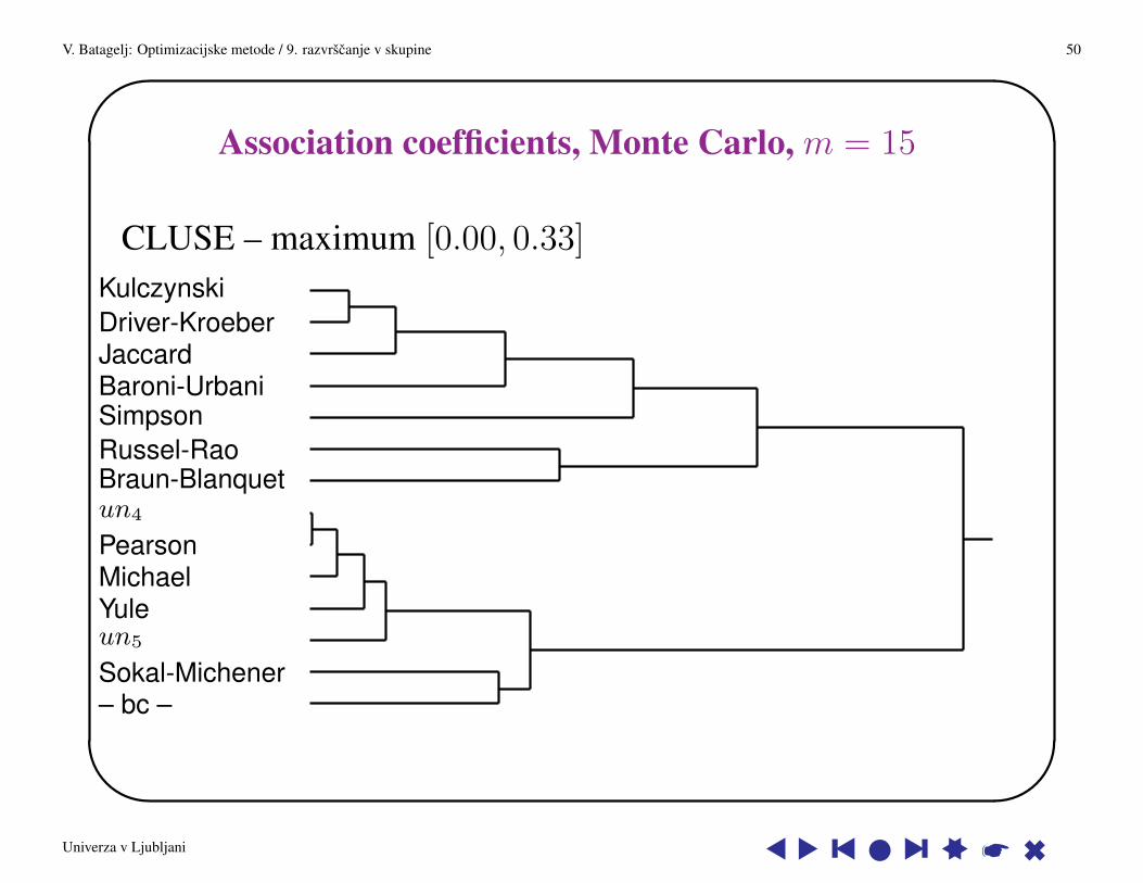
Association coefficients, Monte Carlo, m = 15

CLUSE – maximum [0.00, 0.33]

KulczynskiDriver-KroeberJaccardBaroni-UrbaniSimpsonRussel-RaoBraun-Blanquetun4

PearsonMichaelYuleun5

Sokal-Michener– bc –



&

$

%

InversionsUnfortunately the function hD(C) = D(Cp, Cq), C = Cp ∪ Cq is notalways a level function – for some Ds the inversions, D(Cp, Cq) >

D(Cp ∪ Cq, Cs), are possible.

Batagelj (1981) showed:

Theorem 1.9 hD is a level function for the Lance-Williams procedure (α1,α2, β, γ) iff:

(i) γ + min(α1, α2) ≥ 0

(ii) α1 + α2 ≥ 0

(iii) α1 + α2 + β ≥ 1

The dissimilarity D has the reducibility property (Bruynooghe, 1977) iff

D(Cp, Cq) ≤ t, D(Cp, Cs) ≥ t, D(Cq, Cs) ≥ t ⇒ D(Cp ∪ Cq, Cs) ≥ t

Theorem 1.10 If a dissimilarity D has the reducibility property then hDis a level function.



&

$

%

Adding hierarchical methodsSuppose that we already built a clustering tree T over the set of units U.To add a new unit X to the tree T we start in the root and branch down.Assume that we reached the node corresponding to cluster C, which wasobtained by joining subclusters Cp and Cq . There are three possibilities: orto add X to Cp, or to add X to Cq , or to form a new cluster {X}.

Consider again the ’greedy approximation’ P (C•k) = P (C•k+1) +

D(Cp, Cq) where D(Cp, Cq) = minCu,Cv∈C•k+1D(Cu, Cv) and C•i

are greedy solutions.

Since we wish to minimize the value of criterion P it follows from thegreedy relation that we have to select the case corresponding to the maximalamong values D(Cp∪{X}, Cq), D(Cq ∪{X}, Cp) and D(Cp∪Cq, {X}).

This is a basis for the adding clustering method. We start with a tree on thefirst two units and then successively add to it the remaining units. The unitX is included into all clusters through which we branch it down.



&

$

%

... adding hierarchical methods

tCp

tCq

tC

��X

tCp ∪X

tCq

tC ∪X

��

tCp

tCq ∪X

tC ∪X

AAU t

Cp

tCq

tC

tX

tC ∪XHHj



&

$

%

About the minimal solutions of (Pk, SR)

Theorem 1.11 In the (locally with respect to transitions) minimal cluste-ring for the problem (Pk,SR)

SR. P (C) =∑C∈C

∑X∈C

w(X) · d(X, C)

each unit is assigned to the nearest representative: Let C• be (locally withrespect to transitions) minimal clustering then it holds:

∀Cu ∈ C•∀X ∈ Cu∀Cv ∈ C• \ {Cu} : d(X, Cu) ≤ d(X, Cv)



&

$

%

ProofLet C′ = (C• \ {Cu, Cv}) ∪ {Cu \ {X}, Cv ∪ {X}} be any clustering neighbouring withrespect to transitions to the clustering C• . From the theorem assumptions P (C•) ≤ P (C′)

and the type of criterion function we have:

p(Cu) + p(Cv) ≤ p(Cu \X) + p(Cv ∪X)

and by proposition 1.4.b: ≤ p(Cu)− w(X).d(X, Cu) + p(Cv ∪X).Therefore p(Cv) ≤ p(Cv ∪X)− w(X).d(X, Cu), and

w(X).d(X, Cu) ≤ p(Cv ∪X)− p(Cv) =

= p(Cv ∪X)− (p(Cv) + w(X).d(X, Cv)) + w(X).d(X, Cv)

= w(X).d(X, Cv) + (p(Cv ∪X)−∑

Y∈Cv∪X

w(Y).d(Y, Cv))

By the definition of cluster-error function of type R the second term in the last line is negative.Therefore

≤ w(X).d(X, Cv)

Dividing by w(X) > 0 we finally get

d(X, Cu) ≤ d(X, Cv)



&

$

%

Leaders methodIn order to support our intuition in further development we shall brieflydescribe a simple version of dynamic clusters method – the leaders ork-means method, which is the basis of the ISODATA program (one amongthe most popular clustering programs) and several recent ’data-mining’methods. In the leaders method the criterion function has the form SR.

The basic scheme of leaders method is simple:

determine C0; C := C0;

repeatdetermine for each C ∈ C its leader C;the new clustering C is obtained by assigning each unit

to its nearest leaderuntil leaders stabilize

To obtain a ’good’ solution and an impression of its quality we can repeatthis procedure with different (random) C0.



&

$

%

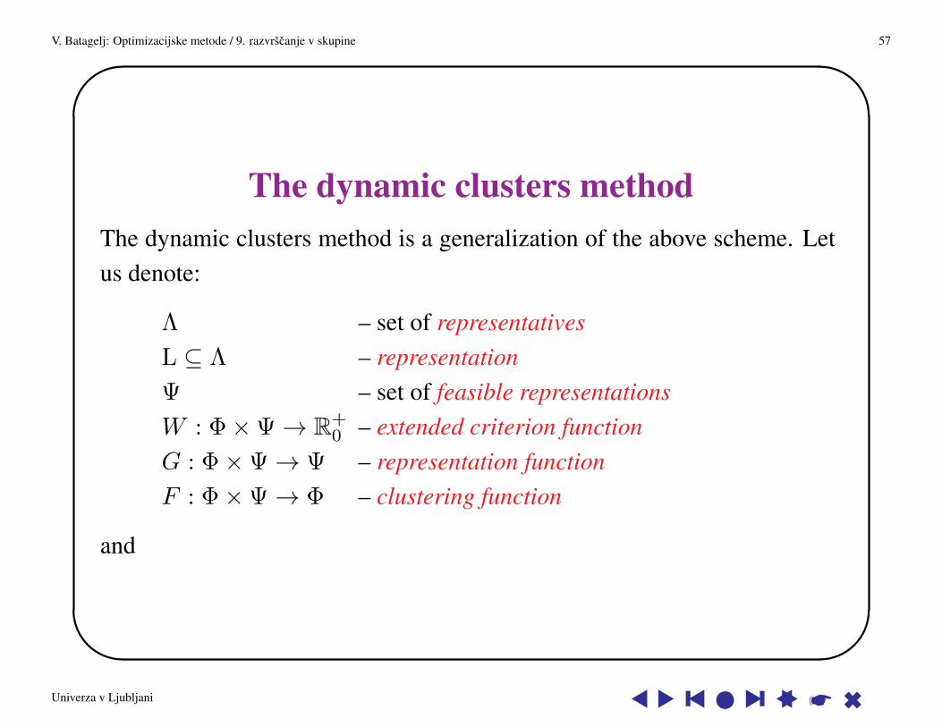
The dynamic clusters methodThe dynamic clusters method is a generalization of the above scheme. Letus denote:

Λ – set of representativesL ⊆ Λ – representationΨ – set of feasible representationsW : Φ×Ψ→ R+

0 – extended criterion functionG : Φ×Ψ→ Ψ – representation functionF : Φ×Ψ→ Φ – clustering function

and



&

$

%

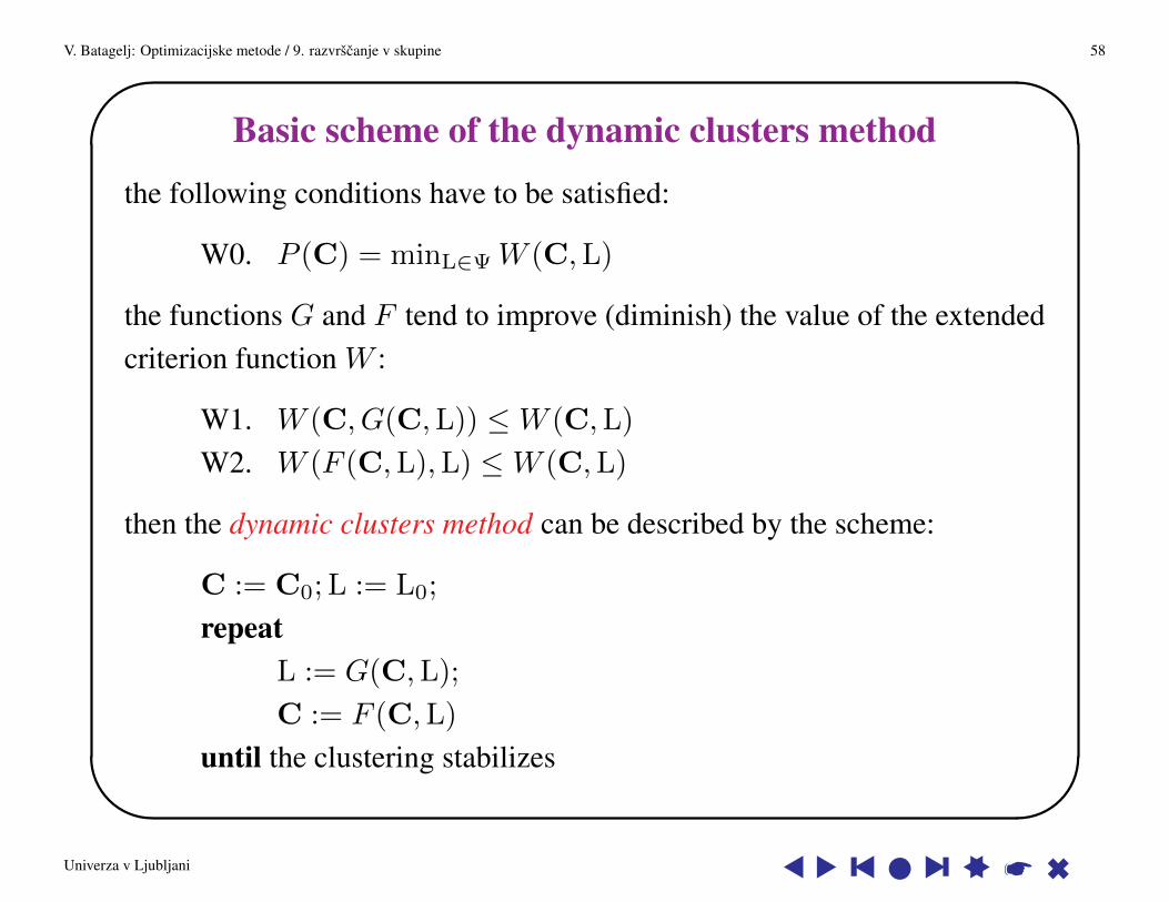
Basic scheme of the dynamic clusters method

the following conditions have to be satisfied:

W0. P (C) = minL∈ΨW (C,L)

the functions G and F tend to improve (diminish) the value of the extendedcriterion function W :

W1. W (C, G(C,L)) ≤W (C,L)

W2. W (F (C,L),L) ≤W (C,L)

then the dynamic clusters method can be described by the scheme:

C := C0; L := L0;

repeatL := G(C,L);

C := F (C,L)

until the clustering stabilizes



&

$

%

Properties of DCM

To this scheme corresponds the sequence vn = (Cn,Ln), n ∈ N determinedby relations

Ln+1 = G(Cn,Ln) and Cn+1 = F (Cn,Ln+1)

and the sequence of values of the extended criterion function un =

W (Cn,Ln). Let us also denote u∗ = P (C∗). Then it holds:

Theorem 1.12 For every n ∈ N, un+1 ≤ un, u∗ ≤ un,and if for k > m, vk = vm then ∀n ≥ m : un = um.

The Theorem 2.6 states that the sequence un is monotonically decreasingand bounded, therefore it is convergent. Note that the limit of un isnot necessarily u∗ – the dynamic clusters method is a local optimizationmethod.



&

$

%

... types of of DCM sequences

Type A: ¬∃k,m ∈ N, k > m : vk = vm

Type B: ∃k,m ∈ N, k > m : vk = vm

Type B0: Type B with k = m+ 1

The DCM sequence (vn) is of type B if

• sets Φ and Ψ are both finite.For example, when we select a representative of C among its members.

• ∃δ > 0 : ∀n ∈ N : (vn+1 6= vn ⇒ un − un+1 > δ)

Because the sets U and consequently Φ are finite we expect from a good dynamicclusters procedure to stabilize in finite number of steps – is of type B.



&

$

%

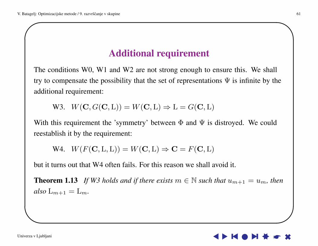
Additional requirementThe conditions W0, W1 and W2 are not strong enough to ensure this. We shalltry to compensate the possibility that the set of representations Ψ is infinite by theadditional requirement:

W3. W (C, G(C,L)) = W (C,L)⇒ L = G(C,L)

With this requirement the ’symmetry’ between Φ and Ψ is distroyed. We couldreestablish it by the requirement:

W4. W (F (C,L,L)) = W (C,L)⇒ C = F (C,L)

but it turns out that W4 often fails. For this reason we shall avoid it.

Theorem 1.13 If W3 holds and if there exists m ∈ N such that um+1 = um, thenalso Lm+1 = Lm.



&

$

%

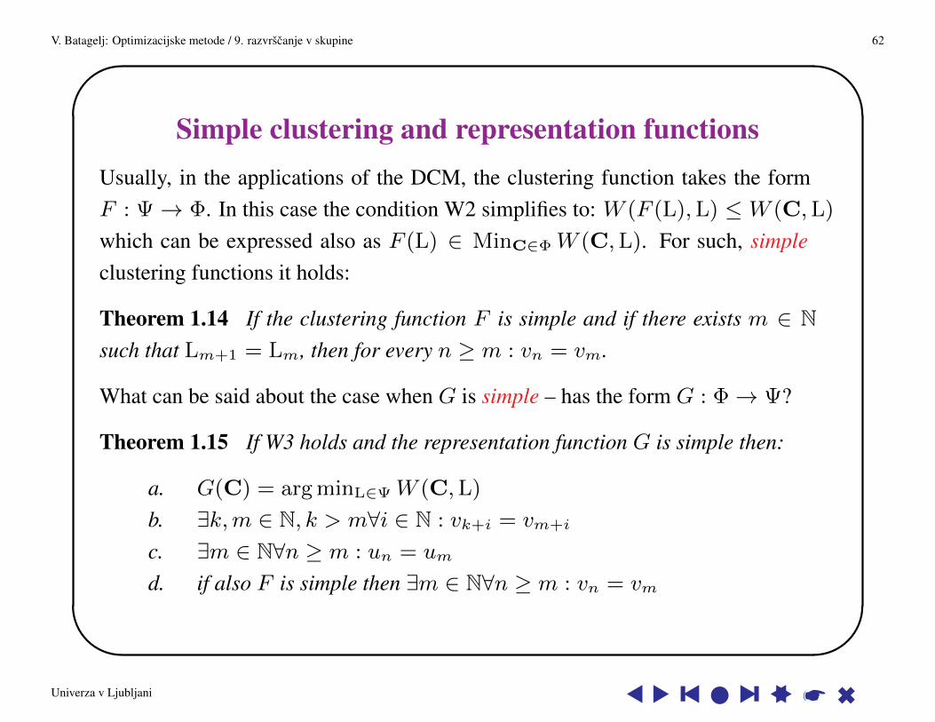
Simple clustering and representation functionsUsually, in the applications of the DCM, the clustering function takes the formF : Ψ→ Φ. In this case the condition W2 simplifies to: W (F (L),L) ≤ W (C,L)

which can be expressed also as F (L) ∈ MinC∈Φ W (C,L). For such, simpleclustering functions it holds:

Theorem 1.14 If the clustering function F is simple and if there exists m ∈ Nsuch that Lm+1 = Lm, then for every n ≥ m : vn = vm.

What can be said about the case when G is simple – has the form G : Φ→ Ψ?

Theorem 1.15 If W3 holds and the representation function G is simple then:

a. G(C) = arg minL∈Ψ W (C,L)

b. ∃k,m ∈ N, k > m∀i ∈ N : vk+i = vm+i

c. ∃m ∈ N∀n ≥ m : un = um

d. if also F is simple then ∃m ∈ N∀n ≥ m : vn = vm



&

$

%

Original DCMIn the original dynamic clusters method (Diday, 1979) both functions F and G aresimple – F : Ψ→ Φ and G : Φ→ Ψ.

We proved, if also W3 holds and the functions F and G are simple, then:

G0. G(C) = argminL∈ΨW (C,L)

andF0. F (L) ∈ MinC∈Φ W (C,L)

In other words, given an extended criterion function W , the relations G0 and F0define an appropriate pair of functions G and F such that the DCM stabilizes infinite number of steps.



&

$

%

Clustering and Networks• clustering with relational constraint

• transforming data into graphs (neighbors)

• clustering of networks; dissimilarities between graphs (networks)

• clustering of vertices / links; dissimilarities between vertices

• clustering in large networks



&

$

%

Clustering with relational constraintSuppose that the units are described by attribute data a: U → [U] and related by abinary relation R ⊆ U×U that determine the relational data (U, R, a).

We want to cluster the units according to the similarity of their descriptions, but alsoconsidering the relation R – it imposes constraints on the set of feasible clusterings,usually in the following form:

Φ(R) = {C ∈ P (U) : each cluster C ∈ C is a subgraph (C,R ∩ C × C) in thein the graph (U, R) of the required type of connectedness}



&

$

%

Some types of relational constraintsWe can define different types of sets of feasible clusterings for the same relation R.Some examples of types of relational constraint Φi(R) are

type of clusterings type of connectedness

Φ1(R) weakly connected units

Φ2(R) weakly connected units that contain at most one center

Φ3(R) strongly connected units

Φ4(R) clique

Φ5(R) the existence of a trail containing all the units of the cluster

A set of units L ⊆ C is a center of cluster C in the clustering of type Φ2(R) iff thesubgraph induced by L is strongly connected and R(L) ∩ (C \ L) = ∅.



&

$

%

Some graphs of different types

s1

s2

s3 s4

��AAAAA�

��

��

a clique

s1

s2

s3

s4 s5

��AAAAAU�

�

��AAAAAU

strongly connected units

s1

s2

s3

s4 s5

��AAAAAU-

�

�

��

AAAAAU

weakly connected units

s1

s2

s3

s4 s5

��AAAAAU�

�

�

weakly connected unitswith a center {1, 2, 4}



&

$

%

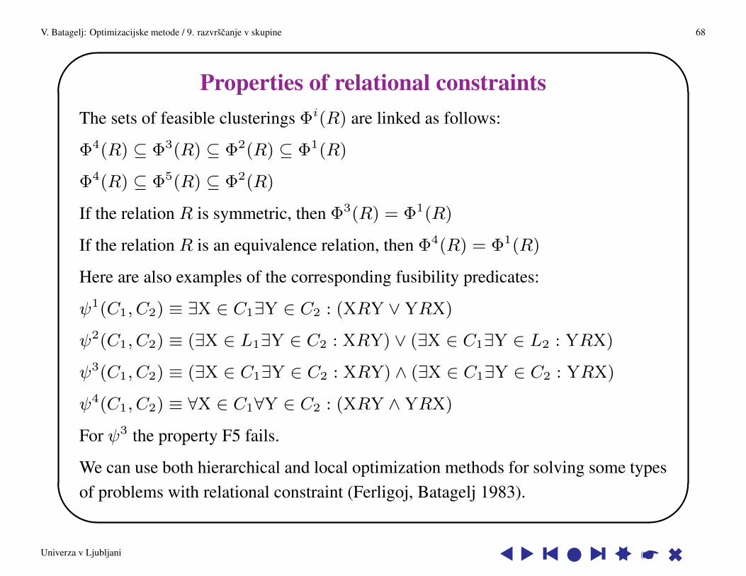
Properties of relational constraintsThe sets of feasible clusterings Φi(R) are linked as follows:

Φ4(R) ⊆ Φ3(R) ⊆ Φ2(R) ⊆ Φ1(R)

Φ4(R) ⊆ Φ5(R) ⊆ Φ2(R)

If the relation R is symmetric, then Φ3(R) = Φ1(R)

If the relation R is an equivalence relation, then Φ4(R) = Φ1(R)

Here are also examples of the corresponding fusibility predicates:

ψ1(C1, C2) ≡ ∃X ∈ C1∃Y ∈ C2 : (XRY ∨YRX)

ψ2(C1, C2) ≡ (∃X ∈ L1∃Y ∈ C2 : XRY) ∨ (∃X ∈ C1∃Y ∈ L2 : YRX)

ψ3(C1, C2) ≡ (∃X ∈ C1∃Y ∈ C2 : XRY) ∧ (∃X ∈ C1∃Y ∈ C2 : YRX)

ψ4(C1, C2) ≡ ∀X ∈ C1∀Y ∈ C2 : (XRY ∧YRX)

For ψ3 the property F5 fails.

We can use both hierarchical and local optimization methods for solving some typesof problems with relational constraint (Ferligoj, Batagelj 1983).



&

$

%

Neighborhood GraphsFor a given dissimilarity d on the set of units U we can define several graphs:

The k nearest neighbors graph GN (k) = (U, A)

(X,Y) ∈ A⇔ Y is among the k closest neighbors of X

By setting for a(X,Y) ∈ A its value to w(a) = d(X,Y) we obtain a network.In the case of equidistant pairs of units we have to decide – or to include them all inthe graph, or specify an additional selection rule.

A special case of the k nearest neighbors graph is the nearest neighbor graphGN (1). We shall denote by G∗NN the graph with included all equidistant pairs, andby GNN a graph where a single nearest neighbor is always selected.

The fixed-radius neighbors graph GB(r) = (U, E)

(X : Y) ∈ E ⇔ d(X,Y) ≤ r

There are several papers on efficient algorithms for determining the neighborhoodgraphs (Fukunaga, Narendra (1975), Dickerson, Eppstein (1996), Chavez & (1999),Murtagh (1999)). These graphs are a bridge between data and network analysis.



&

$

%

Structure and properties of the nearest neighbor graphsLet N = (U, A, w) be a nearest neighbor network. A pair of units X,Y ∈ U arereciprocal nearest neighbors or RNNs iff (X,Y) ∈ A and (Y,X) ∈ A.

Suppose card(U) > 1. Then in N

• every unit/vertex X ∈ U has the outdeg(X) ≥ 1 — there is no isolated unit;

• along every walk the values of w are not increasing.

using these two observations we can show that in N∗NN :

• all the values of w on a closed walk are the same and all its arcs are reciprocal— all arcs between units in a nontrivial (at least 2 units) strong component arereciprocal;

• every maximal (can not be extended) elementary (no arc is repeated) walk endsin a RNNs pair;

• there exists at least one RNNs pair – corresponding to minX,Y∈U,X 6=Y d(X,Y).



&

$

%

Quick agglomerative clustering algorithmsAny graph GNN is a subgraph of G∗NN . Its connected components are directed(acyclic) trees with a single RNNs pair in the root.

Based on the nearest neighbor graph very efficient O(n2) algorithms for agglome-rative clustering for methods with the reducibility property can be built.

chain := [ ]; W := U;while card(W) > 1 do begin

if chain = [ ] then select an arbitrary unit X ∈W else X := last(chain);grow a NN-chain from X until a pair (Y,Z) of RNNs are obtained;agglomerate Y and Z:

T := Y ∪ Z; W := W \ {Y,Z} ∪ {T}; compute D(T,W ),W ∈W

end;

It can be shown that if the clustering method has the reducibility property (minimum,maximum, Ward, . . . ; but not Bock) then the NN-chain remains a NN-chain alsoafter the agglomeration of the RNNs pair.



&

$

%

Clustering of Graphs and NetworksWhen the set of units U consists of graphs (for example chemical molecules)we speak about clustering of graphs (networks). For this purpose we can usestandard clustering approaches provided that we have an appropriate definition ofdissimilarity between graphs.

The first approach is to define a vector description [G] = [g1, g2, . . . , gm] of eachgraph G, and then use some standard dissimilarity δ on Rm to compare thesevectors d(G1,G2) = δ([G1], [G2]). We can get [G], for example, by:

Invariants: compute the values of selected invariants (indices) on each graph(Trinajstic, 1983).

Fragments count: select a collection of subgraphs (fragments), for example triads,and count the number of appearences of each – fragments spectrum.



&

$

%

Invariants and structural propertiesLet Gph be the set of all graphs. An invariant of a graph is a mapping i: Gph→ Rwhich is constant over isomorphic graphs

G ≈ H⇒ i(G) = i(H)

The number of vertices, the number of arcs, the number of edges, maximum degree∆, chromatic number χ, . . . are all graph invariants.

Invariants have an important role in examining the isomorphism of two graphs.

Invariants on families of graphs are called structural properties: Let F ⊆ Gph bea family of graphs. A property i:F → R is structural on F iff

∀G,H ∈ F : (G ≈ H⇒ i(G) = i(H))

A collection I of invariants/structural properties is complete iff

(∀i ∈ I : i(G) = i(H))⇒ G ≈ H

In most cases there is no efficiently computable complete collection.



&

$

%

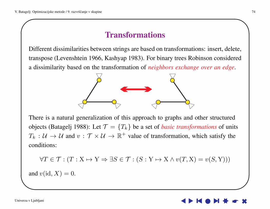
TransformationsDifferent dissimilarities between strings are based on transformations: insert, delete,transpose (Levenshtein 1966, Kashyap 1983). For binary trees Robinson considereda dissimilarity based on the transformation of neighbors exchange over an edge.

There is a natural generalization of this approach to graphs and other structuredobjects (Batagelj 1988): Let T = {Tk} be a set of basic transformations of unitsTk : U → U and v : T × U → R+ value of transformation, which satisfy theconditions:

∀T ∈ T : (T : X 7→ Y ⇒ ∃S ∈ T : (S : Y 7→ X ∧ v(T,X) = v(S,Y)))

and v(id, X) = 0.



&

$

%

Transformations based dissimilaritySuppose that for each pair X,Y ∈ U there exists a finite sequence τ =

(T1, T2, . . . , Tt) such that: τ(X) = Tt ◦ Tt−1 ◦ . . . ◦ T1(X) = Y. Then wecan define:

d(X,Y) = minτ

(v(τ(X)) : τ(X) = Y)

where

v(τ(X)) =

0 τ = id

v(η(T (X))) + v(T,X) τ = η ◦ T

It is easy to verify that so defined dissimilarity d(X,Y) is a distance.



&

$

%

Examples of transformations

Using the transformations G1 and G2 we can transform any pair of connectedsimple graphs one to the other. For triangulations of the plane on n vertices S issuch a transformation.



&

$

%

Clustering in Graphs and NetworksSince in a graph G = (V,L) we have two kinds of objects – vertices and links wecan speak about clustering of vertices and clustering of links. Usually we deal withclustering of vertices.

Again we can use the standard clustering methods provided that we have anappropriate definition of dissimilarity between vertices.

The usual approach is to define a vector description [v] = [t1, t2, . . . , tm] of eachvertex v ∈ V , and then use some standard dissimilarity δ on Rm to compare thesevectors d(u, v) = δ([u], [v]). For some ’nonstandard’ such descriptions see Moody(2001) and Harel, Koren (2001).

We can assign to each vertex v also different neighborhoods

N(v) = {u ∈ V : (v, u) ∈ L}

and other sets. In these cases the dissimilarities between sets are used on them.



&

$

%

Properties of verticesFor a given graph G = (V,L) a property t : V → R is structural iff for everyautomorphism ϕ of G it holds

∀v ∈ V : t(v) = t(ϕ(v))

Examples of such properties are

t(v) = degree (number of neighbors) of vertex vt(v) = number of vertices at distance d from vertex vt(v) = number of triads of type x at vertex v



&

$

%

Properties of pairs of verticesFor a given graph G = (V,L) a property of pairs of vertices q : V × V → R isstructural if for every automorphism ϕ of G it holds

∀u, v ∈ V : q(u, v) = q(ϕ(u), ϕ(v))

Some examples of structural properties of pairs of vertices

q(u, v) = if (u, v) ∈ L then 1 else 0q(u, v) = number of common neighbors of units u and vq(u, v) = length of the shortest path from u to v

Using a selected property of pairs of vertices q we can describe each vertex u with avector

[u] = [q(u, v1), q(u, v2), . . . , q(u, vn), q(v1, u), . . . , q(vn, u)]

and again define the dissimilarity between vertices u, v ∈ V as d(u, v) = δ([u], [v]).



&

$

%

Matrix dissimilaritiesThe following is a list of dissimilarities, used in literature, based on properties ofpairs of vertices for measuring the similarity between vertices vi and vj (p ≥ 0):

Manhattan: dm(vi, vj) =∑ns=1(|qis − qjs|+ |qsi − qsj |)

Euclidean: dE(vi, vj) =√∑n

s=1((qis − qjs)2 + (qsi − qsj)2)

Truncated Man.: ds(vi, vj) =∑n

s=1s 6=i,j

(|qis − qjs|+ |qsi − qsj |)

Truncated Euc.: dS(vi, vj) =√∑n

s=1s 6=i,j

((qis − qjs)2 + (qsi − qsj)2)

Corrected Man.: dc(p)(vi, vj) = ds(vi, vj) + p · (|qii − qjj |+ |qij − qji|)

Corrected Euc.: de(p)(vi, vj) =√dS(vi, vj)2 + p · ((qii − qjj)2 + (qij − qji)2)

Corrected diss.: dC(p)(vi, vj) =√dc(p)(vi, vj)

The corrected dissimilarities with p = 1 should be used.



&

$

%

Graph theory approachesThe basic decomposition of graphs is to (weakly) connected components – partitionof vertices (and links); and to (weakly) biconnected components – partition of links.For both very efficient algorithms exist.

From a network N = (V,L,w) we can get for a treshold t a layer networkN(t) = (V,Lt, w) where Lt = {p ∈ L : w(p) ≥ t}. From it we can get aclustering C(t) with connected components as clusters. For different tresholds theseclusterings form a hierarchy.

In seventies and eighties Matula studied different types of connectivities in graphsand structures they induce. In most cases the algorithms are too demanding to beused on larger graphs. A recent overview of connectivity algorithms was made byEsfahanian.

For directed graphs the fundamental decomposition results can be found in Harary,Norman, and Cartwright (1965).



&

$

%

Decomposition of directed graphsGiven a simple directed graph G = (V,R), R ⊆ V × V we introduce two newrelations, R? (transitive and reflexive closure) and R (transitive closure), based onR:

uR?v := ∃k ∈ N : uRkv and uRv := ∃k ∈ N+ : uRkv

or equivalently

R? =⋃k∈N

Rk and R =⋃k∈N+

Rk

Theorem 1.16a) uRkv iff in the graph G = (V,R) there exists a walk of length k from u to v.b) uR?v iff in the graph G = (V,R) there exists a walk from u to v.c) uRv iff in the graph G = (V,R) there exists a non-null walk from u to v.



&

$

%

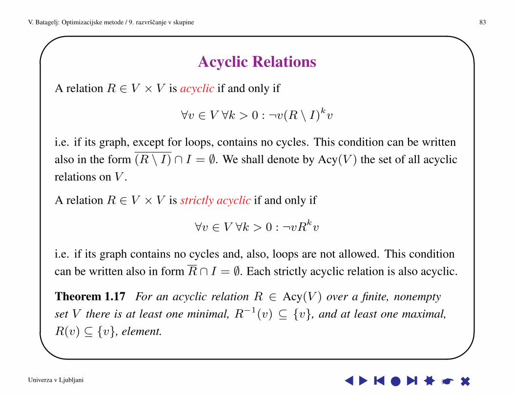
Acyclic RelationsA relation R ∈ V × V is acyclic if and only if

∀v ∈ V ∀k > 0 : ¬v(R \ I)kv

i.e. if its graph, except for loops, contains no cycles. This condition can be writtenalso in the form (R \ I) ∩ I = ∅. We shall denote by Acy(V ) the set of all acyclicrelations on V .

A relation R ∈ V × V is strictly acyclic if and only if

∀v ∈ V ∀k > 0 : ¬vRkv

i.e. if its graph contains no cycles and, also, loops are not allowed. This conditioncan be written also in form R ∩ I = ∅. Each strictly acyclic relation is also acyclic.

Theorem 1.17 For an acyclic relation R ∈ Acy(V ) over a finite, nonemptyset V there is at least one minimal, R−1(v) ⊆ {v}, and at least one maximal,R(v) ⊆ {v}, element.



&

$

%

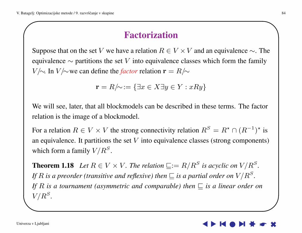
FactorizationSuppose that on the set V we have a relationR ∈ V ×V and an equivalence∼. Theequivalence ∼ partitions the set V into equivalence classes which form the familyV/∼. In V/∼we can define the factor relation r = R/∼

r = R/∼ := {∃x ∈ X∃y ∈ Y : xRy}

We will see, later, that all blockmodels can be described in these terms. The factorrelation is the image of a blockmodel.

For a relation R ∈ V × V the strong connectivity relation RS = R? ∩ (R−1)? isan equivalence. It partitions the set V into equivalence classes (strong components)which form a family V/RS .

Theorem 1.18 Let R ∈ V × V . The relation v:= R/RS is acyclic on V/RS .If R is a preorder (transitive and reflexive) then v is a partial order on V/RS .If R is a tournament (asymmetric and comparable) then v is a linear order onV/RS .



&

$

%

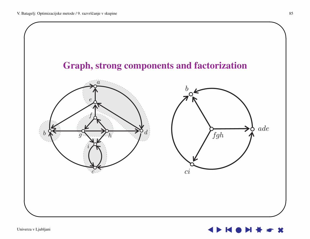
Graph, strong components and factorization



&

$

%

CoresThe notion of a core was introduced by Seidman in 1983.

In a given graph G = (V,L) a subgraph Hk = (W,L|W ) induced by the set W isa k-core or a core of order k iff ∀v ∈ W : degH(v) ≥ k, and Hk is the maximumsubgraph with this property. The core of maximum order is also called the maincore. The core number of vertex v is the highest order of a core that contains thisvertex.

The degree deg(v) can be: in-degree, out-degree, in-degree + out-degree, . . . dete-rmining different types of cores.

In figure an example of cores decomposition of agiven graph is presented. We can see the followingproperties of cores:

• The cores are nested: i < j =⇒ Hj ⊆ Hi

• Cores are not necessarily connected su-bgraphs.



&

$

%

Determining and using coresA very efficient O(m) algorithm (Batagelj, Zaversnik 2002) for determining thecores hierarchy can be built based on the following property:

If from a given graph G = (V,L) we recursively delete all vertices, andlines incident with them, of degree less than k, the remaining graph is thek-core.

The notion of cores can be generalized to networks.

Using cores we can identify the densiest parts of a graph. For revealing theinternal structure of the main core we can use standard clustering procedures ondissimilarities between vertices. Afterwards we can remove the links of the maincore and analyse the residium graph.

Cores can be used also to localize the search for some computationally moredemanding substructures.



&

$

%

Short cyclesA subgraph H = (V ′, A′) of G = (V,A) is cyclic k-gonal if each its vertex andeach its edge belong to at least one cycle of length at most k and at least 2 in H.

A sequence (C1, C2, . . . , Cs) of cycles of length at most k (and at least 2) of G

cyclic k-gonally connects vertex u ∈ V to vertex v ∈ V iff u ∈ C1 and v ∈ Csor u ∈ Cs and v ∈ C1 and V (Ci−1) ∩ V (Ci) 6= ∅, i = 2, . . . s; such sequence iscalled a cyclic k-gonal chain.

A pair of vertices u, v ∈ V is cyclic k-gonally connected iff u = v, or there exists acyclic k-gonal chain that connects u to v.

Theorem 1.19 Cyclic k-gonal connectivity is an equivalence relation on the set ofvertices V .

An arc is cyclic iff it belongs to some cycle (of any length) in the graph G.

Theorem 1.20 If in the graph G for each cyclic arc the length of a shortest cyclethat contains it is at most k then the cyclic k-gonal reduction of G is an acyclicgraph.



&

$

%

Final remarksThe agglomerative methods can be adapted for large sparse networks in sense ofrelational constraint clustering – we have to compute dissimilarities only betweenunits/vertices connected by a link.

The Sollin’s MST algorithm can be very efficiently implemented for large sparsenetworks.


optimizacijske metode / razvr canje v skupine · v. batagelj: optimizacijske metode / 9....

Documents