optimal mass transport and the isoperimetric inequality
TRANSCRIPT

OPTIMAL MASS TRANSPORT AND THE ISOPERIMETRIC
INEQUALITY
KENNETH DEMASON
Abstract. We provide an introduction to optimal mass transport, which has
proved in recent years to be a powerful tool in studying geometric inequalities.In particular, we show a clever application to the isoperimetric inequality.
Contents
1. Introduction 12. Optimal Mass Transport 22.1. The Monge Problem 22.2. The Monge-Kantorovich Formulation 102.3. Brenier Theory 153. The Isoperimetric Inequality 163.1. History of the Isoperimetric Problem 163.2. Solution Using Optimal Mass Transport 174. Acknowledgements 24References 25
1. Introduction
Optimal mass transport has an interesting history. It started off as a problem on“excavations and embankments” – how to transport soil efficiently during the buildingof forts. The original formulation was presented in 1781 by Gaspard Monge while thefield of analysis was blooming.
Due to its difficult nature, no significant progress on the problem was made. In1947, L.V. Kantorovich revisited it and applied it to economics. In this setting,the transport problem becomes one of shipping goods – given production sites anddestinations, how can we efficiently ship goods so each destination receives the amountof goods it needs?
In order to progress transportation theory, Kantorovich established a weaker ver-sion of Monge’s problem. This enabled him to work with a larger class of objectsand obtain significant results. Later on, mathematicians such as Yann Brenier andRobert McCann were able to use Kantorovich’s theory in specific contexts to find nicesolutions to Monge problems.
1

2 KENNETH DEMASON
Optimal mass transport has found continued use since then. In particular, one canuse it to prove the isoperimetric problem. This long standing problem was effectivelysolved in the 1800s. Optimal mass transport can be used to prove it in a simple, cleanway.
This paper focuses on developing the theory of optimal mass transport and show-cases two applications of it in solving the isoperimetric problem.
Section 2 starts by presenting Monge’s problem and several examples. These ex-amples highlight the many ways Monge’s problem can fail to have solutions. We thenstudy Kantorovich’s weaker formulation of Monge’s problem and how it addressesseveral of the previous issues. Finally, we analyze a specific case and show Brenierand McCann’s nice solutions to Monge’s problem.
Section 3 starts with a history of the isoperimetric problem, which provides somenice background to the technical challenges. Following this, we provide two differentproofs of the isoperimetric inequality using optimal mass transport.
Background in measure theory is assumed. The author recommends Chapters 2and 8 of [Mag12]. All information, unless otherwise specified, comes from [Amb00],[Vil03], and [FMP10].
2. Optimal Mass Transport
2.1. The Monge Problem. We begin with the following picture. Suppose we have apile of dirt that we wish to transfer into some hole. We can impose a “cost” associatedwith moving a speck of dirt – say, the distance it travels. Is there a way to move thepile into the hole such that the cost is minimized? Is this mapping unique? This isthe basic formulation of the Monge problem.
In modern language, we can state it as follows. Let f, g : Rn → R be two nonneg-ative L1(Rn) functions such that∫
Rn
f dx =
∫Rn
g dy = 1.
Imagine f as a distribution of dirt – choosing a point x ∈ Rn, f(x) tells you how muchdirt lies on top of x. Imagine g as our target “hole” – choosing a point y ∈ Rn, g(y)tells you how much dirt can fit in the “hole” at y. It is convenient to normalize the to-tal amount of dirt as 1 so that f, g give rise to probability measures µ = fdx, ν = gdy.These measures are precisely those which are absolutely continuous with respect tothe Lebesgue measure. Sometimes, the Monge problem is stated for probability mea-sures in general – we will move freely between the two formulations. The use of x andy is simply cosmetic – x is used for the source space while y is used for the target space.
We wish to find a map T : Rn → Rn such that two conditions hold:
i) The transport condition: For any E ⊂ Rn Borel,∫T−1(E)
f dx =
∫E
g dy.

OPTIMAL MASS TRANSPORT AND THE ISOPERIMETRIC INEQUALITY 3
This essentially tells us that no dirt lying above T−1(E) is lost in the trans-portation, and that all the dirt lying above T−1(E) exactly fills up the holeat E. Such a map fulfilling this condition is called a transport map.
ii) The cost condition: Define the cost of T to be
C(T ) =
∫Rn
|T (x)− x|f(x) dx.
The |T (x) − x| term gives the transport cost for moving mass, while f(x)dxtells us how much mass is being moved. The cost of T is then interpretedas the cost of moving all the mass. For each Monge problem there is anassociated intrinsic cost given by
M(f, g) = infC(T ) | T is a transport map.
This is called the Monge cost, and will sometimes be written as M(µ, ν).The Monge cost measures the minimum theoretical cost. The cost conditionrequires that T satisfies C(T ) = M(f, g). That is, T actually realizes thetheoretical minimum cost. So, T is as efficient as possible.
Such a map T is called an optimal transport map. We remark that the transportcondition may be restated as T#µ = ν, where T#µ(E) := µ(T−1(E)). That is, ν isthe push-forward of µ under T . To see this, one appeals to the well-known change ofvariables formula between µ and ν,∫
T (E)
ϕ dν =
∫E
ϕ T dµ
for measurable ϕ. In light of this, we can rewrite the Monge cost as follows:
M(µ, ν) = infT#µ=ν
∫Rn
|T (x)− x| dµ.
Interestingly, there exists a “duality principle” used to solve optimal mass transportproblems. Let µ, ν be probability measures on Rn such that T#µ = ν. Let u : Rn → Rbe Lipschitz with Lip(u) ≤ 1. Consider the quantity∫
Rn
u dν −∫Rn
u dµ.
Applying the above change of variables formula with u = ϕ yields∫Rn
u T dµ−∫Rn
u dµ.
Then, combining integrals and applying the Lipschitz condition reveals∫Rn
u dν −∫Rn
u dµ =
∫Rn
(u(T (x))− u(x)) dµ(x)
≤∫Rn
|T (x)− x| dµ(x).
So, we see that
infT#µ=ν
∫Rn
|T (x)− x| dµ≥ sup
∫Rn
u dν −∫Rn
u dµ
∣∣∣∣ u : Rn → R, Lip(u) ≤ 1
.

4 KENNETH DEMASON
Thus, if we can find a pair (T, u) where T#µ = ν and u is Lipschitz with Lip(u) ≤ 1such that ∫
Rn
|T (x)− x| dµ =
∫Rn
u dν −∫Rn
u dµ,
then T must be optimal. If not, we would have some T with a lower cost than T . Inturn,
supLip(u)≤1
∫Rn
u dν −∫Rn
u dµ
≥
∫Rn
u dν −∫Rn
u dµ =
∫Rn
|T (x)− x| dµ
>
∫Rn
|T (x)− x| dµ ≥ infT#µ=ν
∫Rn
|T (x)− x| dµ
contradicting the above inf, sup inequality.
Let us look at some examples.
1) Here is a nice, first example. Let N ∈ N. Consider f = χ[0,N ] and g =χ[1,N+1]. An obvious transport is to move [0, N ] laterally to [1, N + 1] viaT (x) = x+ 1. This is depicted below
0 N
1 N + 1
We now want to apply the duality principle to show this is optimal. First letus compute the cost of T :
C(T ) =
∫R|T (x)− x|χ[0,N ] dx
=
∫ N
0
|x+ 1− x| dx = N.
Now consider the 1-Lipschitz function u(x) = x. We have that∫Ru(x)χ[1,N+1] dx−
∫Ru(x)χ[0,N ] dx =
∫ N+1
1
x dx−∫ N
0
x dx
=x2
2
∣∣∣∣N+1
1
− x2
2
∣∣∣∣N0
= N.
Thus, by the duality principle, T is optimal. Is it unique? It turns out that Tis not unique. To see this, imagine [0, N+1] as a bookshelf, with books havinglength 1. Start with N books and one empty slot at [N,N + 1]. Pick up thebook at [0, 1] and move it to the space at [N,N+1]. After the transformation,we still have N books, but an empty slot at [0, 1]. All other books were fixedduring the transformation. Visually,

OPTIMAL MASS TRANSPORT AND THE ISOPERIMETRIC INEQUALITY 5
0 1 N
1 N N + 1
We can describe this map as
T (x) =
x+N x ∈ [0, 1]
x x ∈ (1, N ]
Let us check that this map is also optimal. First, we compute the cost
C(T ) =
∫R|T (x)− x|χ[0,N ] dx
=
∫ 1
0
|x+N − x| dx+
∫ N
1
|x− x| dx = N.
We have already shown that the minimum cost is N , hence T is optimal.
This example highlights the intimate relationship between cost and mass.In the first map, we moved a lot of mass a short distance. In the second map,we moved a small amount of mass a large distance. Yet, both maps wereoptimal.
We can interpolate between the two results. Imagine moving a book oflength [0, d] to [n+ 1−d, n+ 1], and then shifting the rest over – that is, take(d, n] to [1, n+1−d). Each Td is optimal too, hence there are infinitely manyoptimal transport maps.1
2) In some cases, we get lucky and can explicitly compute an optimal transportmap. For this example, let µ = χ[−1,1]dx and ν = δ−1 + δ1. Here, δx isthe dirac measure at x. Note that these are not normalized to 1 to avoidcomplicating the calculations, but one can easily normalize them. Imaginethis setup as having dirt at [−1, 1] and holes at 1,−1. A possible transportis to divide the dirt into [−1, 0) and [0, 1], then move these into the holes at−1, 1 respectively. Explicitly,
T (x) =
−1 x ∈ [−1, 0)
1 x ∈ [0, 1]
We show that T is optimal, and is the unique optimal transport map (up toa.e. equivalence). First, the cost of T is
C(T ) =
∫ 1
−1
|T (x)− x| dx =
∫ 0
−1
|x+ 1| dx+
∫ 1
0
|x− 1| dx = 1.
1These maps have minor technical issues. For example, the first map given, T , sends no point to
1. But, since all of these issues arise on a set of measure zero, we can ignore them.

6 KENNETH DEMASON
Now consider the 1-Lipschitz function u(x) = |x|. Then∫R|x| d(δ−1 + δ1)−
∫ 1
−1
|x| dx = 1 + 1− 1 = 1.
Thus, T is optimal. To show T is the unique optimal transport map, notethat any transport map must be such that T ([−1, 1]) = −1, 1. Thereforewe can write any transport map as
TF (x) =
−1 x ∈ F1 x ∈ F c
where F ⊂ [−1, 1], and the complement is viewed as the relative complementin [−1, 1]. Note that, in order to be a transport map, it must be that 1 =ν(1) = µ(T−1
F 1) = µ(F ). So, |F | = 1. Since F and F c are disjoint, wealso have |F c| = 1. Suppose that TF is optimal, where F 6= [0, 1]. What wewant to show is that F is is “close” to [0, 1], in the sense that it does notspill out into the complement [−1, 0) by too much. So, assume by way ofcontradiction that F is such that F1 = F ∩ [−1, 0) has some measure δ > 0.Then also F2 = F c∩ [0, 1] has measure δ. Now set G = (F \F1)∪F2 – that is,we remove the portion of F which spills out by δ, and fill up the portion whichthe complement subsumed. We now show that C(TG) < C(TF ) contradictingoptimality. By definition
C(TF )− C(TG) =
∫ 1
−1
|TF (x)− x| dx−∫ 1
−1
|TG(x)− x| dx
=
2∑i=1
∫Fi
|TF (x)− x| − |TG(x)− x| dx
Let us look at |TF (x) − x| − |TG(x) − x| on F1 ⊂ [−1, 0). Since TF = 1 onF1, we have that TF (x) − x is positive. On the other hand, TG = −1 on F1
so that TG(x)− x is negative. Consequently, on F1
|TF (x)− x| − |TG(x)− x| = (1− x)− (−(−1− x)) = −2x > 0
Similarly, |TF (x)−x|−|TG(x)−x| is nonnegative on F2 because on it, TF = −1while TG = 1. But F1 and F2 have positive measure, so that the integrals arepositive.
3) It can even be that uniqueness fails so spectacularly that all transport mapsare optimal. For example, let µ a probability measure on R2 supported onx2 = 0 and ν = 1/2(δ(−1,0) + δ(1,0)). Let T : R2 → R2 be a transport map– hence, it takes values in (1, 0), (−1, 0). But, for any (0, a) we have that|(0, a)−T (0, a)| is either |(0, a)− (1, 0)| or |(0, a)− (−1, 0)|. In both cases, the
distances are equal and equal to√
1 + a2. Importantly, this does not dependon T . Hence,
C(T ) =
∫x2=0
|T (x)− x| dµ =
∫x2=0
|x− (1, 0)| dµ
and thus all transport maps have the same cost. In particular they are alloptimal.

OPTIMAL MASS TRANSPORT AND THE ISOPERIMETRIC INEQUALITY 7
4) We may even fail so miserably that we can’t find a single transport map. Letµ = δ0 and ν = 1/2(δ−1 + δ1). Consider E = 1. Then ν(E) = 1/2, butµ(T−1(E)) is either 0 or 1 for any E. Hence, ν(E) 6= µ(T−1(E)), and thereexists no T for which ν = T#µ.
5) Finally, sometimes failure is so subtle that we can find a minimizing sequenceof transport maps, but no optimal transport map. Let µ = χ0×[0,1]dx andν = 1/2(χ−1×[0,1] + χ1×[0,1])dx. Visually, we have the following
All the dirt is concentrated evenly on 0 × [0, 1], and we want to transferit evenly to the two holes on either side, at 1 × [0, 1] and −1 × [0, 1].The “transfer evenly” condition is assumed in order to satisfy the transportcondition – that is, we don’t want to send most of our dirt to one point inthe hole, and spread the rest to the rest of the hole.
Let us define a transport map T1 visually as follows:
So, T1 spreads the top part of our pile evenly into the right hole, and thelower part of our pile evenly into the left pile.Now define T2 and T3 visually as well

8 KENNETH DEMASON
At this point we can start to compute the cost. For each n, we subdivide0 × [0, 1] into 2n evenly spaced regions 0 × [i/2n, (i + 1)/2n] for i =0, 1, ..., 2n − 1. Then for even i, Tn stretches out 0 × [i/2n, (i+ 1)/2n] by afactor of 2 and carries it onto −1 × [i/2n, (i+ 2)/2n]. Tn acts similarly forodd i onto the right hole. Due to the symmetry of Tn, we need only computethe cost to move 0 × [0, 1/2n] and multiply this cost by 2n.
We have that Tn sends (0, x) to (−1, 2x) for 0 ≤ x ≤ 1/2n. Thus the costfor transporting 0 × [0, 1/2n] is
C =
∫ 1/2n
0
√1 + x2 dx =
1
2
(x√
1 + x2 + arcsinh(x)) ∣∣∣∣1/2n
0
=1
2
(1
2n
√1 +
1
22n+ arcsinh
(1
2n
)).
Then the cost of Tn is
C(Tn) = 2nC =1
2
(√1 +
1
22n+ 2n arcsinh
(1
2n
)).
Observe that C(Tn) is monotone decreasing and approaches 1. But if we tryto take a limit of Tn we get something like
where each point (0, x) ∈ 0 × [0, 1] is split in half and sent to (1, x) and(−1, x). Each split portion travels a distance of 1, so in total it is as if (0, x)travels a distance of 1. This rationale shows that C(T ) would be 1, as ex-pected. However, limTn is not a map! We cannot send a point simultaneouslyto two different points. Although limTn is not a map, it actually turns outto be the correct picture in mind for solving this optimal mass transportproblem.
OPTIMAL MASS TRANSPORT AND THE ISOPERIMETRIC INEQUALITY 9
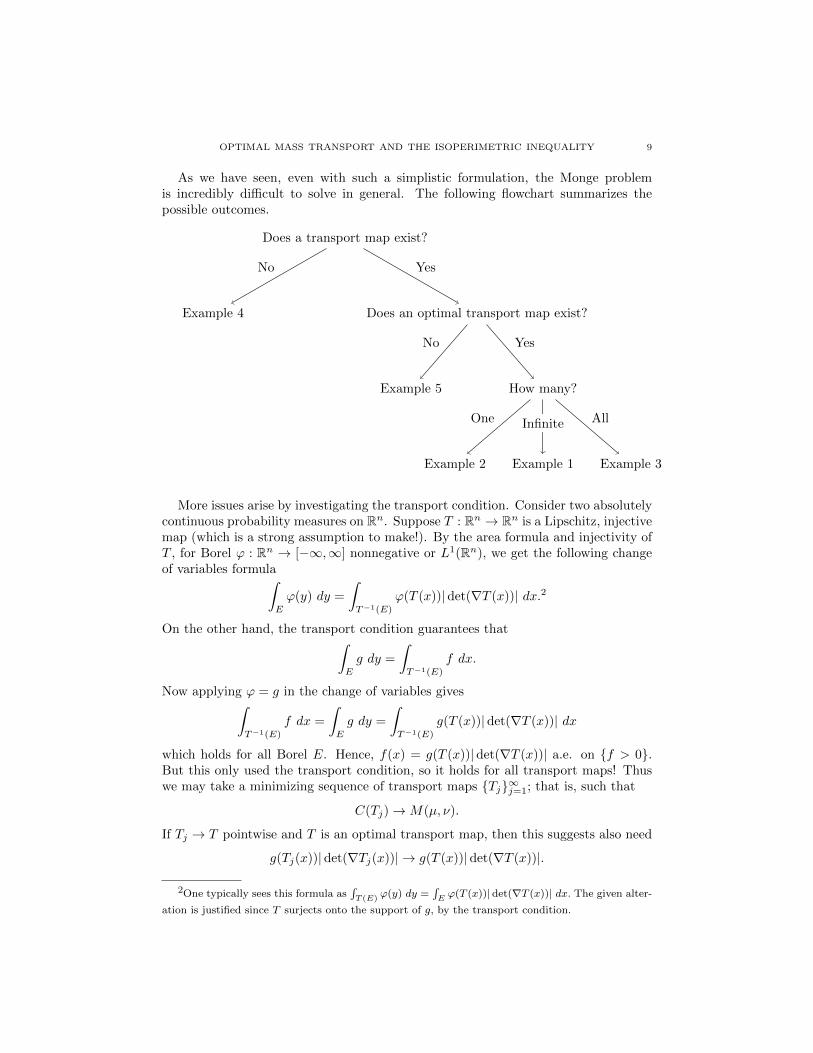
As we have seen, even with such a simplistic formulation, the Monge problemis incredibly difficult to solve in general. The following flowchart summarizes thepossible outcomes.
Does a transport map exist?
Example 4
No
Does an optimal transport map exist?
Example 5
No
How many?
Example 2
One
Example 1 Example 3
All
Yes
Yes
Infinite
More issues arise by investigating the transport condition. Consider two absolutelycontinuous probability measures on Rn. Suppose T : Rn → Rn is a Lipschitz, injectivemap (which is a strong assumption to make!). By the area formula and injectivity ofT , for Borel ϕ : Rn → [−∞,∞] nonnegative or L1(Rn), we get the following changeof variables formula∫
E
ϕ(y) dy =
∫T−1(E)
ϕ(T (x))|det(∇T (x))| dx.2
On the other hand, the transport condition guarantees that∫E
g dy =
∫T−1(E)
f dx.
Now applying ϕ = g in the change of variables gives∫T−1(E)
f dx =
∫E
g dy =
∫T−1(E)
g(T (x))|det(∇T (x))| dx
which holds for all Borel E. Hence, f(x) = g(T (x))|det(∇T (x))| a.e. on f > 0.But this only used the transport condition, so it holds for all transport maps! Thuswe may take a minimizing sequence of transport maps Tj∞j=1; that is, such that
C(Tj)→M(µ, ν).
If Tj → T pointwise and T is an optimal transport map, then this suggests also need
g(Tj(x))|det(∇Tj(x))| → g(T (x))|det(∇T (x))|.
2One typically sees this formula as∫T (E) ϕ(y) dy =
∫E ϕ(T (x))| det(∇T (x))| dx. The given alter-
ation is justified since T surjects onto the support of g, by the transport condition.

10 KENNETH DEMASON
and therefore ∇Tj → ∇T pointwise too. Unlike solving variational problems likeminimizing Dirichlet energy, we do not a priori have any good control over ∇Tj .
Naturally, one might ask: If the Monge problem is so difficult to solve, why careabout it? First, it turns out that relaxing some conditions of the Monge problemproduces reasonable existence conditions. As in Example 5, if we could “split mass”,we would have a solution – this is known as the Monge-Kantorovich formulation.It turns out that using different cost functions, like c(x, y) = |x − y|2 instead ofc(x, y) = |x − y|, also helps. Second, even in the cases where we cannot find anexplicit solution, it is still useful to find transport maps. We will see an example ofthis in Section 3 with the Knothe map.
2.2. The Monge-Kantorovich Formulation. The notion of “splitting mass” willnow be formalized. We thus deviate from transport maps, and look instead the so-called transport plans.
Definition 2.1. Let µ, ν be probability measures on X, Y respectively. We call aprobability measure γ on X × Y a transport plan if
π0#γ = µ and π1#γ = ν.
In this context, we call µ and ν the marginals of γ.
How do we interpret this? The product space X × Y is seen as follows: there ismass at points x ∈ X and holes at y ∈ Y . The pair (x, y) tells us that mass from xcan be sent to y. The measure dγ(x, y) tells us how much mass was sent to y from x.In general then for A ⊂ X, the marginal condition gives∫
A×Ydγ(x, y) =
∫A
dµ(x).
That is, there is an amount of mass at A, given by the right hand side. This massneeds to be conserved no matter where it is sent, so that none is lost. The integralon the left hand side looks at all the mass that came from A, so that equality impliesnone is lost.
Next let us look at X × y with a fixed y ∈ Y . For each x ∈ X, some amountof mass (possibly none) is sent to y. Integrating over X tells us how much mass intotal from X is sent to the point y in the hole Y . We need each part of the hole tobe filled, and ν(y) tells us how much mass can fit there. In general, for B ⊂ Y thesecond marginal condition guarantees∫
X×Bdγ(x, y) =
∫B
dν(y).
That is, all the mass sent to B from X is equal to the amount of space available atB in Y .
The important part of γ is its support, which dictates where mass is sent to. Thatis to say if dγ(x, y) = 0 then no mass is transferred from x to y. It is visualized asfollows.
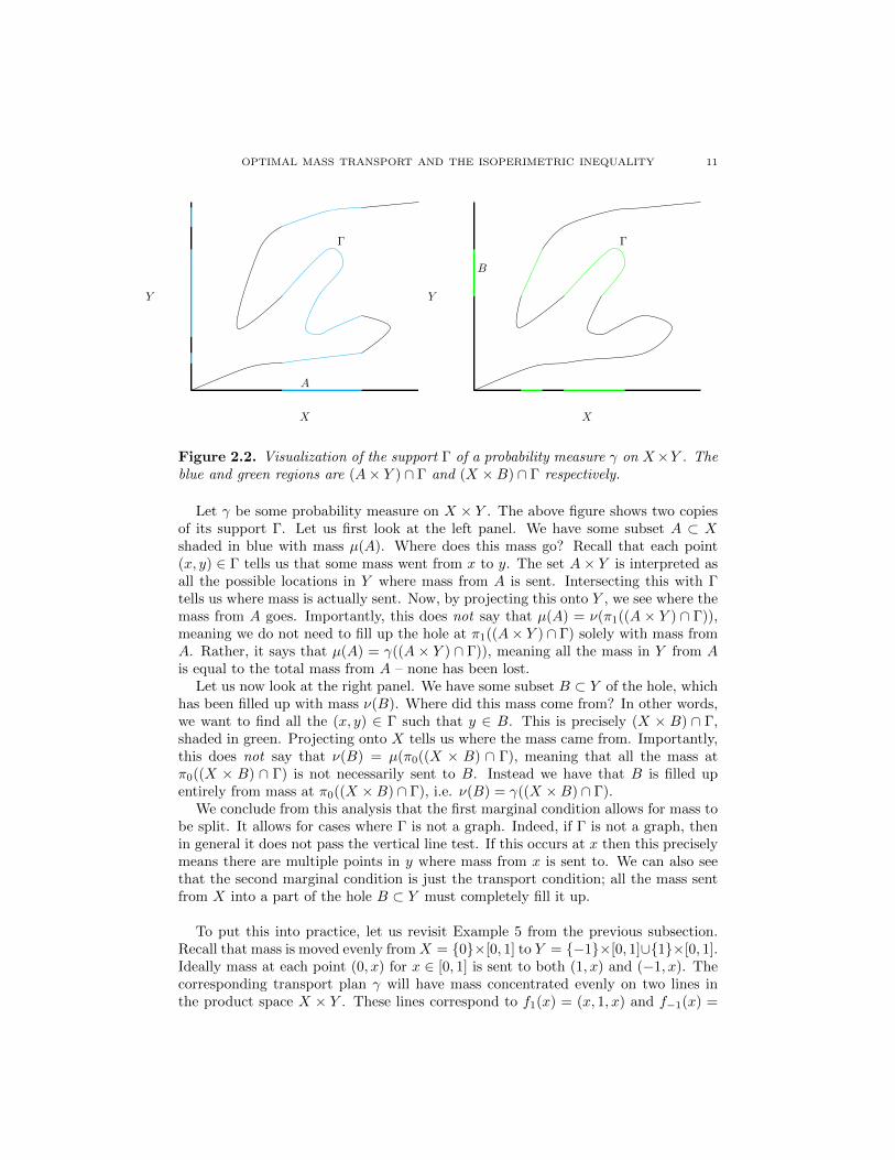
OPTIMAL MASS TRANSPORT AND THE ISOPERIMETRIC INEQUALITY 11
A
Γ
X
Y
B
Γ
X
Y
Figure 2.2. Visualization of the support Γ of a probability measure γ on X×Y . Theblue and green regions are (A× Y ) ∩ Γ and (X ×B) ∩ Γ respectively.
Let γ be some probability measure on X × Y . The above figure shows two copiesof its support Γ. Let us first look at the left panel. We have some subset A ⊂ Xshaded in blue with mass µ(A). Where does this mass go? Recall that each point(x, y) ∈ Γ tells us that some mass went from x to y. The set A× Y is interpreted asall the possible locations in Y where mass from A is sent. Intersecting this with Γtells us where mass is actually sent. Now, by projecting this onto Y , we see where themass from A goes. Importantly, this does not say that µ(A) = ν(π1((A × Y ) ∩ Γ)),meaning we do not need to fill up the hole at π1((A× Y ) ∩ Γ) solely with mass fromA. Rather, it says that µ(A) = γ((A × Y ) ∩ Γ)), meaning all the mass in Y from Ais equal to the total mass from A – none has been lost.
Let us now look at the right panel. We have some subset B ⊂ Y of the hole, whichhas been filled up with mass ν(B). Where did this mass come from? In other words,we want to find all the (x, y) ∈ Γ such that y ∈ B. This is precisely (X × B) ∩ Γ,shaded in green. Projecting onto X tells us where the mass came from. Importantly,this does not say that ν(B) = µ(π0((X × B) ∩ Γ), meaning that all the mass atπ0((X × B) ∩ Γ) is not necessarily sent to B. Instead we have that B is filled upentirely from mass at π0((X ×B) ∩ Γ), i.e. ν(B) = γ((X ×B) ∩ Γ).
We conclude from this analysis that the first marginal condition allows for mass tobe split. It allows for cases where Γ is not a graph. Indeed, if Γ is not a graph, thenin general it does not pass the vertical line test. If this occurs at x then this preciselymeans there are multiple points in y where mass from x is sent to. We can also seethat the second marginal condition is just the transport condition; all the mass sentfrom X into a part of the hole B ⊂ Y must completely fill it up.
To put this into practice, let us revisit Example 5 from the previous subsection.Recall that mass is moved evenly from X = 0×[0, 1] to Y = −1×[0, 1]∪1×[0, 1].Ideally mass at each point (0, x) for x ∈ [0, 1] is sent to both (1, x) and (−1, x). Thecorresponding transport plan γ will have mass concentrated evenly on two lines inthe product space X × Y . These lines correspond to f1(x) = (x, 1, x) and f−1(x) =
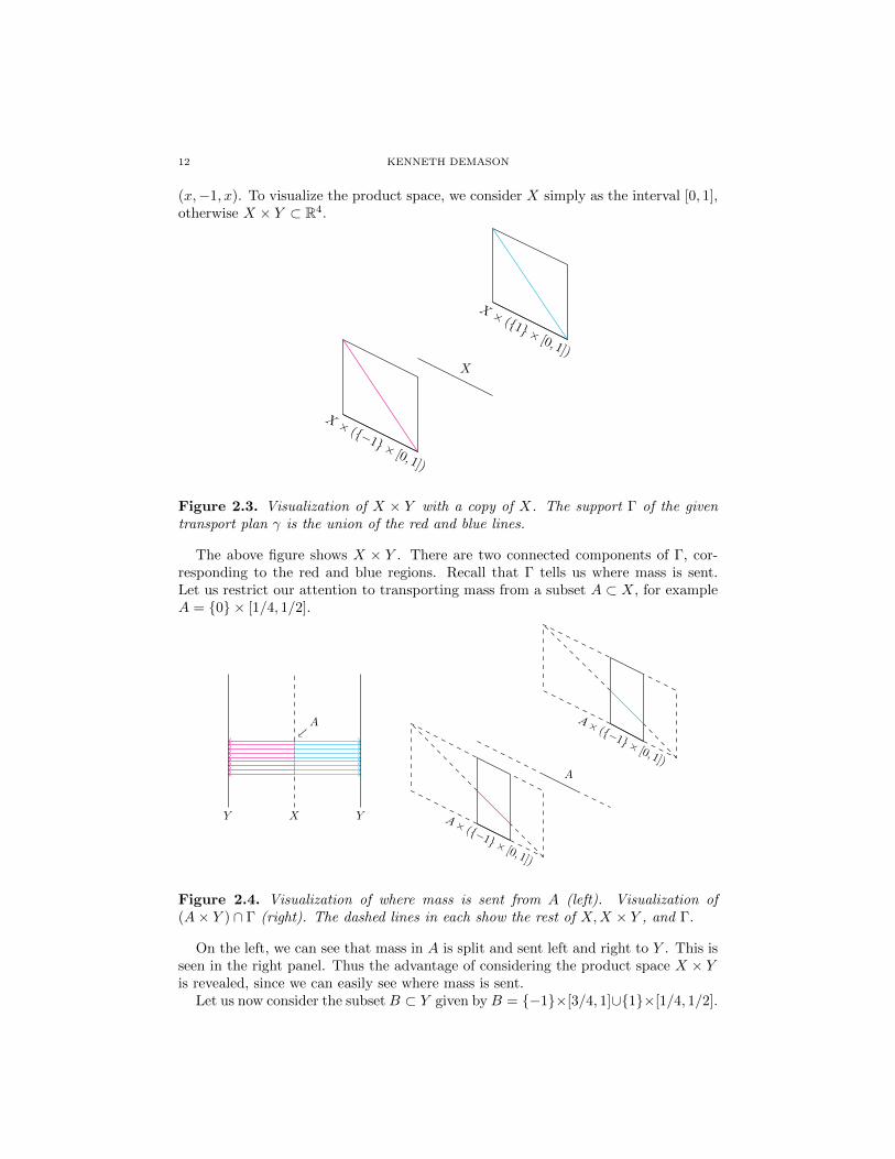
12 KENNETH DEMASON
(x,−1, x). To visualize the product space, we consider X simply as the interval [0, 1],otherwise X × Y ⊂ R4.
X
X × (−1 × [0, 1])
X × (1 × [0, 1])
Figure 2.3. Visualization of X × Y with a copy of X. The support Γ of the giventransport plan γ is the union of the red and blue lines.
The above figure shows X × Y . There are two connected components of Γ, cor-responding to the red and blue regions. Recall that Γ tells us where mass is sent.Let us restrict our attention to transporting mass from a subset A ⊂ X, for exampleA = 0 × [1/4, 1/2].
Y X Y
A
A
A× (−1 × [0, 1])
A× (−1 × [0, 1])
Figure 2.4. Visualization of where mass is sent from A (left). Visualization of(A× Y ) ∩ Γ (right). The dashed lines in each show the rest of X,X × Y , and Γ.
On the left, we can see that mass in A is split and sent left and right to Y . This isseen in the right panel. Thus the advantage of considering the product space X × Yis revealed, since we can easily see where mass is sent.
Let us now consider the subset B ⊂ Y given by B = −1×[3/4, 1]∪1×[1/4, 1/2].
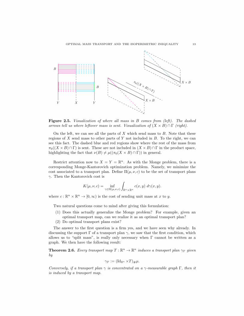
OPTIMAL MASS TRANSPORT AND THE ISOPERIMETRIC INEQUALITY 13
Y X Y
B
B
π0 ((X ×B) ∩ Γ)
X ×B
X ×B
Figure 2.5. Visualization of where all mass in B comes from (left). The dashedarrows tell us where leftover mass is sent. Visualization of (X ×B) ∩ Γ (right).
On the left, we can see all the parts of X which send mass to B. Note that theseregions of X send mass to other parts of Y not included in B. To the right, we cansee this fact. The dashed blue and red regions show where the rest of the mass fromπ0((X ×B)∩Γ) is sent. These are not included in (X ×B)∩Γ in the product space,highlighting the fact that ν(B) 6= µ((π0(X ×B) ∩ Γ)) in general.
Restrict attention now to X = Y = Rn. As with the Monge problem, there is acorresponding Monge-Kantorovich optimization problem. Namely, we minimize thecost associated to a transport plan. Define Π(µ, ν, c) to be the set of transport plansγ. Then the Kantorovich cost is
K(µ, ν, c) = infγ∈Π(µ,ν,c)
∫Rn×Rn
c(x, y) dγ(x, y).
where c : Rn × Rn → [0,∞) is the cost of sending unit mass at x to y.
Two natural questions come to mind after giving this formulation:
(1) Does this actually generalize the Monge problem? For example, given anoptimal transport map, can we realize it as an optimal transport plan?
(2) Do optimal transport plans exist?
The answer to the first question is a firm yes, and we have seen why already. Indiscussing the support Γ of a transport plan γ, we saw that the first condition, whichallows us to “split mass”, is really only necessary when Γ cannot be written as agraph. We then have the following result:
Theorem 2.6. Every transport map T : Rn → Rn induces a transport plan γT givenby
γT := (IdRn ×T )#µ.
Conversely, if a transport plan γ is concentrated on a γ-measurable graph Γ, then itis induced by a transport map.

14 KENNETH DEMASON
Proof. To verify the first part, we first prove the following. If f, g : Rn → Rn aremeasurable functions then
(f g)#µ = f#g#µ.
To see this, let E ⊂ Rn be Borel. Then,
f#(g#µ(E)) = (g#µ)(f−1(E)) = µ(g−1(f−1(E))) = µ((f g)−1(E)).
Next, observe that π0 (IdRn × T ) = IdRn . It follows that
π0#γT = π0#(IdRn ×T )#µ = (IdRn)#µ = µ.
Similarly, π1 (IdRn × T ) = T so that
π1#γT = π1#(IdRn ×T )#µ = T#µ = ν
since T is a transport plan.The proof of the converse is beyond the scope of these notes, but can be found in
[Amb00]. The key point is that Γ is a graph, so that we can construct a transportmap that does not split mass.
To answer the second question, observe first that there always exist transport plans.Clearly, γ = µ× ν is a suitable transport plan. In contrast, a general Monge problemmay not have a transport map. Moreover, Theorem 2.6 tells us that for each transportmap T we have a corresponding transport plan γT . Note that
C(γT ) =
∫Rn×Rn
c(x, y) dγT (x, y) =
∫Rn
c(x, T (x)) dµ = C(T )
so that γT and T have the same cost. This implies that M(µ, ν, c) ≥ K(µ, ν, c), sinceK(µ, ν, c) is an infimum over a possibly larger set.
These facts suggest that the Monge-Kantorovich formulation is weaker than theMonge formulation. A tenant of analysis is, in the search for solutions, to pass weakerclass of objects, solve there, and then upgrade the solution. The following theoremasserts that solutions to the Monge-Kantorovich problem exist.
Theorem 2.7. Let µ, ν be probability measures on Rn. Let c : Rn × Rn → [0,∞) belower semi-continuous. Then there exists an optimal plan γ in Π(µ, ν, c).
Proof. A sketch of the proof is provided. The key idea is to use a form of convergenceknown as narrow convergence. This is slightly stronger than weak-∗ convergence.Note that if µk is a sequence of Radon measures with supk µk(Br(0)) < ∞ for allr > 0, then there exists a convergent weak-∗ subsequence.
Given a minimizing sequence γj ⊂ Π(µ, ν, c), we can extract a weak-∗ subse-quence. This can be upgraded to a narrow convergent subsequence using the finite-ness of µ, ν. Then, show that the convergent measure γ is in Π(µ, ν, c) using severalequivalent criterion for narrow convergence. Finally, it remains to show that γ isoptimal – this follows from the fact that we chose a minimizing sequence.
So, we can solve in the weaker class of objects – transport plans. Can we upgradethese? If an optimal γ takes the special form in Theorem 2.6, that is γ = (IdRn×T )#µ

OPTIMAL MASS TRANSPORT AND THE ISOPERIMETRIC INEQUALITY 15
for a transport map T , then
M(µ, ν, c) ≥ K(µ, ν, c) =
∫Rn×Rn
c(x, y) d((IdRn × T )#µ)
=
∫Rn
c(x, T (x)) dµ(x) ≥M(µ, ν, c).
Hence, T is actually optimal. This forms the central idea of Brenier’s theory, whichwe will review next.
Before continuing, recall the useful duality principle in the Monge problem forfinding optimal transport maps. It turns out there is a corresponding duality principlefor the Monge-Kantorovich formulation. We state it here:
Theorem 2.8 (Duality principle). Let α, β : Rn → R be Borel maps such that
α(x) + β(y) ≤ c(x, y)
for all x, y ∈ Rn. Define A the collection of pairs (α, β) of these maps. Then underthe conditions for the Monge-Kantorovich formulation,
K(µ, ν, c) ≤ sup(α,β)∈A
∫Rn
α(x) dµ(x) +
∫Rn
β(y) dν(y)
.
Notice that this reduces to the original duality principle by taking α = u, β = −uand c(x, y) = |x − y|. Then the condition α(x) + β(y) ≤ c(x, y) guarantees that u isa 1-Lipschitz function.
2.3. Brenier Theory. Here we specialize to the case of the quadratic cost c(x, y) =|x − y|2 and µ, ν absolutely continuous probability measures with finite second mo-ments. To give some intuition, we first define the notion of c-convexity:
Definition 2.9. A function f : Rn → R ∪ ∞ is said to be c-convex if for somefunction α : Rn → R ∪ ∞ we have
f(x) = supy∈Rn
α(y)− c(x, y)
for all x ∈ Rn and f is not uniformly ∞.
Formally, we must allow f to take infinite values. We have defined c-convexity forgeneral costs, but what does it mean when c(x, y) = |x− y|2? Observe the following∫
Rn×Rn
|x|2 dγ(x, y) =
∫Rn
|x|2 dµ(x)
if γ ∈ Π(µ, ν, c). So, if µ has finite second moment, this is a constant independent ofγ. Then, we have that∫
Rn×Rn
|x− y|2 dγ(x, y) =
∫Rn
|x|2 dµ(x) +
∫Rn
|y|2 dν(y)− 2
∫Rn×Rn
〈x, y〉 dγ(x, y).
Since the second moments are finite and independent of γ, it follows that γ is optimalin Π(µ, ν, |x− y|2) if and only if it is optimal in Π(µ, ν,−〈x, y〉).
But, c-convexity for c = −〈x, y〉 is precisely convex and lower-semicontinuous.This follows since the sup of affine functions (of the form a+ 〈x, b〉 for constants a, b)is convex and lower-semicontinuous. So, c-convexity is a natural generalization ofconvexity. The role it plays takes significant time to establish, but the main takeaway
16 KENNETH DEMASON
is that when the cost is convex functions have special properties which can be utilizedin the quadratic case.
Now, given a Kantorovich problem K(µ, ν, c) recall that if γ = (IdRn × T )#µ isoptimal for a transport map T , then T is optimal. Thus, we should study the structureof optimal plans. We have the following theorem to help us with this endeavor
Theorem 2.10 (Brenier). Let µ, ν be absolutely continuous probability measures onRn with respect to Lebesgue measure. Further assume that µ, ν have finite secondmoments. Then for the cost c(x, y) = |x− y|2 there exists a unique optimal transportplan of the form
γ = (IdRn ×∇f)#µ
where f : Rn → R ∪ ∞ is a convex function.
In this case, we call ∇f a Brenier map. Some slight care needs to be taken in orderfor this to make sense. Indeed, f may not be differentiable everywhere. Let F be itsset of differentiability points, which is a Borel set. Then
(∇f)#(µ)(Rn) = µ(∇f−1(Rn)) = µ(F )
since ∇f is only defined on F . Then, it is possible that the pushforward is not aprobability measure!
But if f is convex, it is locally Lipschitz, and hence by Rademacher’s theoremm(Ω \ F ) = 0. Here, Ω = Int(Dom(f)), where Dom(f) = x ∈ Rn | f(x) <∞. Onecan show that f is finite a.e. so that µ is concentrated on Ω. Since µ is absolutelycontinuous to Lebesgue measure, we see that µ(Rn \ F ) = 0. So, µ is concentratedon F , and the pushforward is a probability measure.
One can ask whether we can weaken the hypotheses to omit finiteness of the secondmoments. Robert McCann proved that this was the case.
Theorem 2.11 (McCann). Let µ, ν be probability measures on Rn absolutely contin-uous to Lebesgue measure. Further suppose that µ does not give mass to small sets.Then, the conclusion of Brenier’s theorem holds.
The proof uses a nice implicit function theorem for convex functions (instead ofdifferentiable functions!). The nontechnical requirement that “µ does not give massto small sets” can be made technical by introducing (n − 1)-rectifiable sets. This,however, is beyond the scope of the paper. We direct the interested reader to [Vil03]for proofs of these – see Theorem 2.32 in the book.
As a concluding remark, all of the above theory has been developed for probabilitymeasures absolutely continuous to Lebesgue measure. This was motivated by imag-ining the Radon-Nikodym derivatives dµ/dx and dν/dx as a pile of dirt and a hole,respectively. This gives some physical interpretation to the problem, but it is notnecessary.
3. The Isoperimetric Inequality
3.1. History of the Isoperimetric Problem. We begin our discussion of theisoperimetric inequality with a legend about its origin. We travel back several cen-turies, to 825 BC and the city of Tyre. Dido’s husband Sychaeus was just murderedby her brother, and king of Tyre, Pygmalion. She flees Tyre with some followersand, heading westward, lands at what would become Carthage on the coast of north
OPTIMAL MASS TRANSPORT AND THE ISOPERIMETRIC INEQUALITY 17
Africa. She bargains with a local ruler to obtain land, who sells her some oxhide. Heexplains that she can have all the land she can enclose within the oxhide.
Dido cut the oxhide into thin strips and sewed them together. She was now facedwith the following problem: Dido wants to enclose the most area possible with acertain boundary length. She uses the strips to draw a semicircle bordering the coast,which maximizes the enclosed area. Effectively, Dido has solved the first isoperimetricproblem, and with it founds the prosperous Carthage.
The first step towards proving the isoperimetric problem came from the Greeks.Though his work is lost, Zenodorus (non-rigorously) proved the following in the 100sBC.
Theorem 3.1 (Zenodorus). The following hold:
i) Among regular polygons with the same perimeter, that which has more sideshas greater area.
ii) A circle with the same perimeter as a regular polygon has greater area.iii) The regular n-gon maximizes area among all n-gons with the same perimeter.
See [Kli72] for an account of this. As far as the Greeks were concerned, this solvedthe isoperimetric problem. But there were crucial flaws – for one, there are moreextravagant shapes than just polygons and circles. Another more glaring issue isthat Zenodorus assumes the existence of a maximizer in his proof. The isoperimetricproblem then lay dormant for many centuries while mathematicians were unable toresolve these.
In 1842, Jakob Steiner miraculously gave five different proofs of the improvedisoperimetric problem: among all closed plane curves with a prescribed length, thecircle bounds the greatest area. The five proofs are similar and contain many ofthe same ideas, namely they all revolve around techniques to increase the area whilekeeping the perimeter fixed. Doing this requires many symmetrization arguments,and the end result is a circle.
However, like the Greeks before him, Steiner presupposed existence of a maximizer.Indeed, he crucially assumed that his symmetrization arguments never halt, and wecan keep performing them until (in the limit) we get a circle. Though this was obviousto Steiner, he never formally proved it.
In 1879, Weierstrass proved existence using the calculus of variations, finally com-pleting a rigorous solution of the isoperimetric problem. In the decades afterwards,several mathematicians returned to Steiner’s original proofs and showed they werevalid (namely, the limit process holds). A detailed account of this history can befound here [Bla05].
3.2. Solution Using Optimal Mass Transport. We now turn to proving theisoperimetric problem in higher dimensions using optimal mass transport. We firstnote that the original statements of the isoperimetric problem had fixed perimeter,and we were trying to find a solution which maximized volume. We can reformulatethis to instead look at sets with fixed volume, and minimize perimeter. Here is howwe can see this: Suppose that Σ is a solution only to the above “dual” isoperimetricproblem. Then, there exists a set Σ with the same perimeter, but greater area (since
Σ does not solve the classical isoperimetric problem). Now rescale Σ so that it has

18 KENNETH DEMASON
the same area as Σ. It follows that the rescaled Σ must have smaller perimeter thanΣ, a contradiction. We now present the solution.
Theorem 3.2 (Isoperimetric Inequality). Let E ⊂ Rn be bounded with smooth bound-ary. Then
P (E) ≥ P (Br)
where r is such that Vol(Br) = Vol(E). Furthermore, equality holds if and only ifE = Br up to translation and modification on a set of measure zero.
The isoperimetric inequality as stated is readable and has the easy interpretationthat, among all sets with the same volume, the ball minimizes perimeter. However,it is not scale invariant. That is, if we want to scale up E by some factor, we wouldneed to find a new radius to compare Br and E. We wish to avoid this, and we can.
Theorem 3.3 (Scale Invariant Isoperimetric Inequality). Let E ⊂ Rn be boundedwith smooth boundary. Then,
P (E) ≥ nVol(E)(n−1)/n Vol(B1)1/n.
To see that this is scale invariant, consider E 7→ rE. Then,
P (rE) = rn−1P (E) ≥ rn−1nVol(E)(n−1)/n Vol(B1)1/n = nVol(rE)(n−1)/n Vol(B1)1/n.
We now show how to derive this form.
Proof. First, there exists an r such that Vol(E) = Vol(Br). Now, observe that
div(Id(x)) =
n∑k=1
∂ Id
∂xk= n
since all the partial derivatives are 1. Hence, by the divergence theorem we have
nVol(B1) =
∫B1
div(Id) =
∫∂B1
〈x, νB1(x)〉 = P (B1)
since νB1(x) = x and 〈x, x〉 = |x|2 = 1. Substituting this gives
P (E) ≥ P (Br) = rn−1P (B1) = rn−1nVol(B1).
We can actually find what r is! Since Vol(E) = Vol(Br), it follows that rn =Vol(E)/Vol(B1). Hence,
P (E) ≥ nVol(E)(n−1)/n Vol(B1)1/n
as desired.
We remark that the two inequalities are obviously equivalent. For if Vol(E) =Vol(B1), then the right hand side becomes nVol(B1) = P (B1).
We present two different proofs of the isoperimetric inequality. The first utilizes atransport map, showing that even non-optimal maps have utility. The second appre-ciates the power of an optimal transport map.
This first proof was given by Gromov using what is known as the Knothe map.The first step of the proof is to construct the Knothe map in general for absolutelycontinuous measures. In the second step we prove the isoperimetric inequality.
OPTIMAL MASS TRANSPORT AND THE ISOPERIMETRIC INEQUALITY 19
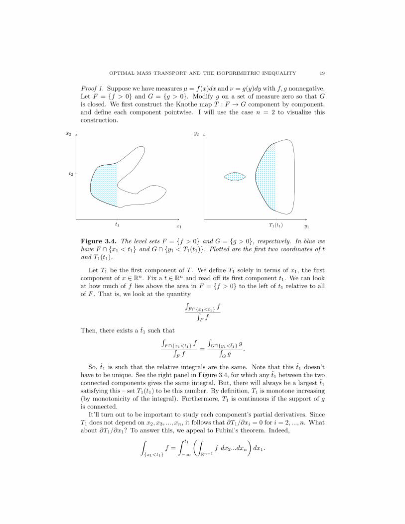
Proof 1. Suppose we have measures µ = f(x)dx and ν = g(y)dy with f, g nonnegative.Let F = f > 0 and G = g > 0. Modify g on a set of measure zero so that Gis closed. We first construct the Knothe map T : F → G component by component,and define each component pointwise. I will use the case n = 2 to visualize thisconstruction.
t1
t2
x1
x2
T1(t1) y1
y2
Figure 3.4. The level sets F = f > 0 and G = g > 0, respectively. In blue wehave F ∩ x1 < t1 and G ∩ y1 < T1(t1). Plotted are the first two coordinates of tand T1(t1).
Let T1 be the first component of T . We define T1 solely in terms of x1, the firstcomponent of x ∈ Rn. Fix a t ∈ Rn and read off its first component t1. We can lookat how much of f lies above the area in F = f > 0 to the left of t1 relative to allof F . That is, we look at the quantity∫
F∩x1<t1 f∫Ff
Then, there exists a t1 such that∫F∩x1<t1 f∫
Ff
=
∫G∩y1<t1 g∫
Gg
.
So, t1 is such that the relative integrals are the same. Note that this t1 doesn’thave to be unique. See the right panel in Figure 3.4, for which any t1 between the twoconnected components gives the same integral. But, there will always be a largest t1satisfying this – set T1(t1) to be this number. By definition, T1 is monotone increasing(by monotonicity of the integral). Furthermore, T1 is continuous if the support of gis connected.
It’ll turn out to be important to study each component’s partial derivatives. SinceT1 does not depend on x2, x3, ..., xn, it follows that ∂T1/∂xi = 0 for i = 2, ..., n. Whatabout ∂T1/∂x1? To answer this, we appeal to Fubini’s theorem. Indeed,∫
x1<t1f =
∫ t1
−∞
(∫Rn−1
f dx2...dxn
)dx1.
20 KENNETH DEMASON
By taking the x1-derivative of this and applying the fundamental theorem of calculus,we obtain
∂
∂x1
∫x1<t1
f =
∫Rn−1
f(t1, x2, ..., xn) dx2...dxn =
∫x1=t1
f(x1, x2, ..., xn) dx2...dxn.
On the other hand, if we do the same thing for the integral of g we get
∂
∂x1
∫y1<T1(t1)
g =∂
∂x1
∫ T1(t1)
−∞
(∫Rn−1
g dy2...dyn
)dy1
=∂T1
∂x1(t1)
∫Rn−1
g(T1(t1), y2, ..., yn) dy2...dyn
=∂T1
∂x1(t1)
∫y1=T1(t1)
g(y1, y2, ..., yn) dy2...dyn
by an application of the chain rule and the fundamental theorem of calculus. Now,by definition of T1(t1),
∂
∂x1
(∫F∩x1<t1 f∫
Ff
)=
∂
∂x1
(∫G∩y1<T1(t1) g∫
Gg
).
where the denominators are just some constants. Hence, after rearranging,
∂T1
∂x1(t1, x2, ..., xn) =
∫Gg∫
Ff
∫x1=t1 f∫y1=T1(t1) g
.
This partial derivative is positive due to monotonicity of T1.
We now define T2, which will depend on x1 and x2. Here’s the idea: we used theordering on R to define T1. But, in Rn, there is no such ordering. Having chosen t1and T1(t1), we can look at F1 = F ∩ x1 = t1 and G1 = G ∩ y1 = T1(t1). Thesesets are n− 1 dimension, so we can drop down a dimension and do almost the samething with t2 in place of t1 and F1, G1 in place of F,G. See the figure below.
t1
t2 F1
x1
x2
T1(t1)
T2(t1, t2)
G1
y1
y2
Figure 3.5. The sets F1 = F ∩ x1 = t1 and G1 = G ∩ y1 = T1(t1) contained inF,G respectively. In blue we have the sets F1 ∩ x2 < t2 and G1 ∩ y2 < T2(t1, t2).Plotted are the first two coordinates of t as well as T1(t1) and T2(t1, t2).
OPTIMAL MASS TRANSPORT AND THE ISOPERIMETRIC INEQUALITY 21
As before, it could be that ∫F1
f 6=∫G1
g
so we have to add a normalizing factor.3 Thus, we define T2(t1, t2) as the greatestnumber such that ∫
F1∩x2<t2 f∫F1f
=
∫G1∩y2<T2(t1,t2) g∫
G1g
.
So, F1 ∩ x2 < t2 and G1 ∩ y2 < T2(t1, t2) cover the same relative area of F1, G1
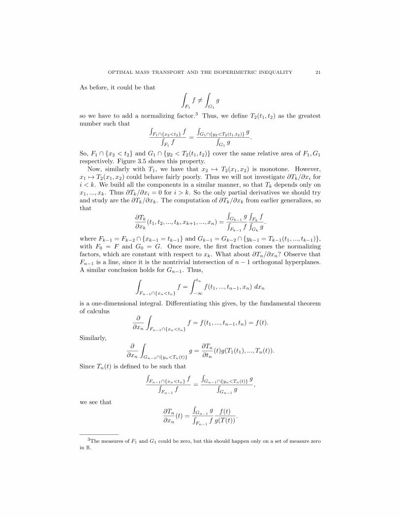
respectively. Figure 3.5 shows this property.Now, similarly with T1, we have that x2 7→ T2(x1, x2) is monotone. However,
x1 7→ T2(x1, x2) could behave fairly poorly. Thus we will not investigate ∂Tk/∂xi fori < k. We build all the components in a similar manner, so that Tk depends only onx1, ..., xk. Thus ∂Tk/∂xi = 0 for i > k. So the only partial derivatives we should tryand study are the ∂Tk/∂xk. The computation of ∂Tk/∂xk from earlier generalizes, sothat
∂Tk∂xk
(t1, t2, ..., tk, xk+1, ..., xn) =
∫Gk−1
g∫Fk−1
f
∫Fkf∫
Gkg.
where Fk−1 = Fk−2 ∩ xk−1 = tk−1 and Gk−1 = Gk−2 ∩ yk−1 = Tk−1(t1, ..., tk−1),with F0 = F and G0 = G. Once more, the first fraction comes the normalizingfactors, which are constant with respect to xk. What about ∂Tn/∂xn? Observe thatFn−1 is a line, since it is the nontrivial intersection of n− 1 orthogonal hyperplanes.A similar conclusion holds for Gn−1. Thus,∫
Fn−1∩xn<tnf =
∫ tn
−∞f(t1, ..., tn−1, xn) dxn
is a one-dimensional integral. Differentiating this gives, by the fundamental theoremof calculus
∂
∂xn
∫Fn−1∩xn<tn
f = f(t1, ..., tn−1, tn) = f(t).
Similarly,
∂
∂xn
∫Gn−1∩yn<Tn(t)
g =∂Tn∂tn
(t)g(T1(t1), ..., Tn(t)).
Since Tn(t) is defined to be such that∫Fn−1∩xn<tn f∫
Fn−1f
=
∫Gn−1∩yn<Tn(t) g∫
Gn−1g
,
we see that
∂Tn∂xn
(t) =
∫Gn−1
g∫Fn−1
f
f(t)
g(T (t)).
3The measures of F1 and G1 could be zero, but this should happen only on a set of measure zero
in R.
22 KENNETH DEMASON
In total, we have that ∇T is an upper triangular matrix. Thus the determinant is
det(∇T )(x) =
n∏k=1
∂Tk∂xk
=
(∫Gg∫
Ff
∫F1f∫
G1g
)(∫G1g∫
F1f
∫F2f∫
G2g
)...
(∫Gn−2
g∫Fn−2
f
∫Fn−1
f∫Gn−1
g
)(∫Gn−1
g∫Fn−1
f
f(t)
g(t)
)
=ν(G)
µ(F )
f(x)
g(T (x))> 0
for a.e. x ∈ F . Since T maps F into G, and g > 0 on G, we see that this is welldefined. Clearly this construction depends on an initial choice of basis for Rn (becausethe half-spaces generated will be different). We note here that T is a transport map,albeit not an optimal transport map! Thus, it can still be fruitful to study transportmaps in general.
As a remark, the above construction simplifies when f = χF and g = χG formeasureable sets F,G. In this case, we define Tk+1(t1, ..., tk+1) for k = 0, ..., n− 1 by
Hn−k(Fk ∩ xk+1 < tk+1)Hn−k(Fk)
=Hn−k(Gk ∩ yk+1 < Tk+1(t1, ..., tk+1))
Hn−k(Gk).
We turn to prove the isoperimetric inequality using the Knothe map. Considerthe case when f = χE and g = χB1
, where E ⊂ Rn is bounded and such thatVol(E) = Vol(B1). Note that T transports E onto B1. So, T : E → B1, and inparticular |T | ≤ 1. Moreover, by the above formula for the determinant,
(det∇T )(x) =Vol(B1)
Vol(E)
χE(x)
χB1(T (x))
=χE(x)
χB1(T (x))
= 1
for a.e. x ∈ E. Trivially, we have that
Vol(E) =
∫E
1 =
∫E
det∇T =
∫E
(det∇T )1/n
since we’re just modifying something equal to 1. Now, we can apply the inequality ofarithmetic and geometric means (AM-GM), which states for λk ≥ 0 that(
n∏k=1
λk
)1/n
≤ 1
n
n∑k=1
λk
with equality if and only if all λk are equal. The eigenvalues for ∇T are ∂Tk/∂xk > 0since ∇T is upper triangular. Thus applying AM-GM to the eigenvalues λk gives
Vol(E) ≤ 1
n
∫E
n∑k=1
∂Tk∂xk
=1
n
∫E
div T.
We now apply the divergence theorem to obtain
Vol(E) ≤ 1
n
∫∂E
〈T, νE〉,

OPTIMAL MASS TRANSPORT AND THE ISOPERIMETRIC INEQUALITY 23
where νE is the outer unit normal of E. Since |T | ≤ 1, and |νE | = 1 by definition, wesuggestively use Cauchy-Schwarz
Vol(E) ≤ 1
n
∫∂E
|T ||νE | ≤1
n
∫∂E
1 =1
nP (E).
We proved earlier that
nVol(B1) = P (B1).
Substituting this into the estimate for Vol(E) gives
P (B1) = nVol(B1) = nVol(E) ≤ P (E)
as desired. The general case holds by scaling.
To solve the rigidity part of the theorem, note that if P (B1) = P (E) then theinequality from AM-GM is an equality. Hence, all the partial derivatives are equal,and in particular equal to 1. This is not enough to conclude that E = B1 (up to a setof measure zero, translations, rotations, etc.). The details will be omitted, but theessence is to construct infinitely many Knothe maps in each direction ν ∈ Sn−1 andforce E to lie in between the two supporting hyperplanes of B1 with unit normalsν,−ν.
One major complication in Gromov’s proof is the need to use infinitely manytransport maps to show that P (E) = P (B1) implies E = B1 modulo the appropriatecongruences. We present an alternative proof using Brenier maps.
Proof 2. Note that the Knothe map had three key properties when f = χE andg = χB1 ,
i) det∇T = 1,ii) |T | ≤ 1,iii) div T ≥ n(det∇T )1/n.
Any map T with these properties can be used in the first proof to reach the sameconclusion by following the exact same steps. Let E ⊂ Rn be bounded and suchthat Vol(E) = Vol(B1). Consider now the optimal transport problem sending µ =χE/Vol(E)dx to ν = χB1
/Vol(B1)dy with cost c(x, y) = |x − y|2. It follows thatthese are probability measures absolutely continuous to the Lebesgue measure. Notethat µ, ν have finite second moments since E,B1 are bounded. Thus, we can applyBrenier’s theorem and conclude that there exists a convex ϕ : Rn → R ∪ ∞ suchthat (∇ϕ)#µ = ν. Since ϕ is convex it follows that ∇2ϕ is a positive semi-definitesymmetric matrix. Thus, |det∇ϕ| = det∇ϕ. We saw at the beginning that transportmaps obey
f(x) = g(∇ϕ(x))|det(∇2ϕ)| = g(∇ϕ(x)) det(∇2ϕ).
Rearranging this yields
det(∇2ϕ) =χE(x)
χB1(∇ϕ(x))
Vol(B1)
Vol(E)=
χE(x)
χB1(∇ϕ(x))
so that condition i) is satisfied for a.e. x ∈ E, so long as ∇ϕ maps into B1.
24 KENNETH DEMASON
To prove ii), due to the transport condition
1 = ν(B1) = µ(∇(ϕ)−1(B1)) =1
Vol(E)
∫∇(ϕ)−1(B1)∩E
1 ≤ 1
so that ∇ϕ maps E into B1. Thus, |∇ϕ| ≤ 1, and conditions i) and ii) are satisfied.
Finally, let λk be the eigenvalues of ∇2ϕ. Observe that for all k, λk ≥ 0 since ϕ isconvex (in contrast to the previous example, where they were positive by monotonic-ity) Then,
div(∇ϕ) =
n∑k=1
∂2ϕ/∂x2k = tr(∇2ϕ) =
n∑k=1
λk
= n
(1
n
n∑k=1
λk
)≥ n
(n∏k=1
λk
)1/n
= n(det(∇2ϕ))1/n.
So, condition iii) is satisfied. Thus, we can prove the isoperimetric inequality usingthe Brenier map ∇ϕ.
We can now prove that equality holds if and only if E = B1 modulo some congru-ences. Since ∇2ϕ is symmetric it is diagonalizable. Assuming that P (E) = P (B1),we once more obtain that all the eigenvalues λk of ∇2ϕ must be equal, and sincedet(∇2ϕ) = 1, in particular are all equal to 1. Thus ∇2ϕ is similar to the identitymatrix. Hence the transport map ∇ϕ is some translation. This proof easily showsthe inequality is sharp. Crucially, nonnegativity of the eigenvalues was obtained fromϕ being a convex function.
As a concluding remark, we can actually prove the scale invariant form of theisoperimetric inequality via a slight modification in the above proofs. Namely, wesimply drop the assumption that Vol(E) = Vol(B1). Because of this property i)changes to det∇T = Vol(B1)/Vol(E) while properties ii) and iii) remain the same.Then,
P (E) =
∫∂E
1 ≥∫∂E
〈T, νE〉 =
∫E
div T ≥ n∫E
(det∇T )1/n
= nVol(E)Vol(B1)1/n
Vol(E)1/n= nVol(E)(n−1)/n Vol(B1)1/n
still using Cauchy-Schwarz with property ii), the divergence theorem, and propertiesiii) and i) (modified), in that order.
4. Acknowledgements
I am thankful for my mentor, Dr. Robin Neumayer, for many deep and enjoyableconversations. Her guidance not only helped solidify my knowledge of optimal masstransportation but also inspired me to continue work in geometric variational prob-lems. I would also like to thank Peter May for allowing me to (informally) participatein UChicago’s 2020 REU.

OPTIMAL MASS TRANSPORT AND THE ISOPERIMETRIC INEQUALITY 25
References
[Amb00] Luigi Ambrosio. Lecture notes on optimal transport problems. https://cvgmt.sns.it/
media/doc/paper/1008/trasporto.pdf, 2000.
[Bla05] Viktor Blasjo. The isoperimetric problem. The American Mathematical Monthly,
112(6):526–566, 2005.[FMP10] A. Figalli, F. Maggi, and A. Pratelli. A mass transportation approach to quantitative
isoperimetric inequalities. Inv. Math., 182(1):167–211, 2010.[Kli72] Morris Kline. Mathematical Thought from Modern to Ancient Times. Oxford University
Press, 1972.
[Mag12] Francesco Maggi. Sets of Finite Perimeter and Geometric Variational Problems: An In-troduction to Geometric Measure Theory, volume 135 of Cambridge Studies in Advanced
Mathematics. Cambridge University Press, 2012.
[Roc70] R.T. Rockafellar. Convex Analysis. Princeton Landmarks in Mathematics. American Math-ematical Society, 1970.
[Vil03] Cedric Villani. Topics in Optimal Transportation, volume 58 of Graduate Studies in Math-
ematics. American Mathematical Society, 2003.