Optimal Liquidity and Economic Stability

Linghui Han and Il Houng Lee

WP/12/135

© 2012 International Monetary Fund WP/12/135

IMF Working Paper

Asia and Pacific Department

Optimal Liquidity and Economic Stability

Prepared by Linghui Han and Il Houng Lee1

Authorized for distribution by Il Houng Lee

May 2012

Abstract

Monetary aggregates are now much less used as policy instruments as identifying the right measure has become difficult and interest rate transmission has worked well in an increasingly complex financial system. In this process, little attention was paid to the potential spillover of excess liquidity. This paper suggests a notional level of “optimal” liquidity beyond which asset prices will start to rise faster than the GDP deflator, thereby creating a gap between the face value and the real purchasing value of financial assets and widen the wedge in income between those with capital stock and those living on salaries. Such divergence will eventually lead to an abrupt and disorderly adjustment of the asset value, with repercussions on the real sector.

JEL Classification Numbers:C82, E22, E50

Keywords: monetary policy; liquidity; dynamic panel

Author’s E-Mail Address: ilee@imf.org; hanlinghui92@gmail.com

1 Linghui Han is a fellow at the Research Institute of Fiscal Science, Ministry of Finance and the National Institute for Fiscal Studies, Tsinghua University, P.R. China and Il Houng Lee is the IMF Senior Resident Representative in China. The authors thank Masahiko Takeda, Murtaza Syed, and Malhar Shyam Nabar for useful comments and suggestions. They are also grateful to Jingfang Hao for excellent assistance in the compilation of data.

This Working Paper should not be reported as representing the views of the IMF. The views expressed in this Working Paper are those of the author(s) and do not necessarily represent those of the IMF or IMF policy. Working Papers describe research in progress by the author(s) and are published to elicit comments and to further debate.

2

Contents Page

I. Introduction ............................................................................................................................3 

II. Defining Liquidity and Optimality ........................................................................................5 

III. Testing for Causality between Liquidity and Prices ..........................................................10 

IV. Relationship between liquidity and consumption ..............................................................12 

V. Summary and Conclusion ...................................................................................................14 

References ................................................................................................................................16  Annexes A. Sources of Data and Estimation Results .............................................................................18 B. Relationship Liquidity and Demand ...................................................................................20 

I. INTRODUCTION

The definition of money has evolved but is still anchored on the notion that money provides ready access to current and future goods and services, i.e., cash value. Liquidity is often defined as assets that can be easily converted into cash, and now includes most financial assets as financial innovations and financial deepening have enabled them to be readily converted into money. In this regard, the definition of money can be broadened to equal liquidity. The traditional conceptual framework of money and price dynamics, however, has not kept up with the expanding concept of money. The formalization of the conceptual framework of the role of money M probably started with the infamous Fisher’s “equation of exchange” MV = PT, where M is money, V is velocity, P the price level and T the level of transactions. Since it assumes that V and T are fixed and M is exogenous, an increase in M will lead to an exact proportional increase in the price level. The Cambridge school highlights money’s role as a store-of-wealth (including for precautionary motive) and defines M/P = kY where k is the Cambridge constant capturing the opportunity cost of money (interest). Thus, k is not institutionally fixed but changing. This is equivalent to Fisher's equation if one recognizes that real income (Y) and transactions (T) are identical and k=1/V. Keynes further enriched the Cambridge equation by providing three motives for money, i.e., transaction, precautionary, and speculative. Money demand is affected by income and interest rates, so that Md = L(r, Y) where r is the average of rate of return on illiquid assets. The basic propositions are L’(r) < 0 due to the opportunity cost, and L’(Y) > 0. These motives provide the basis for holding a larger amount of money within the economy. In Milton Friedman’s general form of money demand Md introduces the generalized portfolio constraint (Md - Ms) + (Bd - Bs) + (Yd - Ys) = 0 which connects the goods market with the money and bond markets. A monetary expansion (Ms) can be offset by an excess demand for goods. Then output Ys will rise and money demand Md will rise so that the goods market and money market are brought back into equilibrium. Increasingly less attention is paid to the interconnectedness between money and the real sector, and thus on a mechanism for correction if money exceeds a notional optimal level. In large part, this is because the relationship between money in the classical sense and the real economy has weakened with the expansion of financial market instruments. Money M as used in Fisher’s equation is now only a fraction of instruments of transaction and as a store of value. Similarly, Friedman’s generalized portfolio constraint no longer captures the complexity of the current financial system. Indeed, M (narrowly defined money) is only relevant in influencing short term liquidity condition, and hence the short term interest rate. Accordingly, in several countries monetary aggregates are now playing a relatively minor role in monetary policy formulations. The former Federal Reserve Governor L. Mayer noted that “money plays no role in today’s consensus macro model.” Consistent with this view, the Federal Open Market Committee does not specify a monetary aggregate as a target. Indeed, Bernanke (2006) stated that targeting monetary aggregates have not been effective in “constraining policy or in reducing inflation.” He attributes this to the recurrent instability in the relationship between money demand framework associated with deregulation and

4

financial innovation. While the Federal Reserve continues to monitor and analyze monetary developments, he argued against heavy reliance on monetary aggregate in policy formulation. These views are supported by Woodford (2007), who reviewed inflation models with no roles for money and suggested that these models are not inconsistent with elementary economic principles. Using a basic new Keynesian model, he showed (implicitly) that central banks’ inflation target credibility and their reaction function (policy rate) are adequate in setting a path for the price level without explicitly modeling a role for money. In Europe, on the other hand, monetary aggregates are not fully dismissed in policy formulation. As noted by Kahn and Benolkin (2007), the European Central Bank continues to regard money as one of the factors determining inflation outlook over the medium term. Even then, its focus is more on identifying an appropriate money demand framework and less on redefining money that better captures the growing complexity of the financial market. These said, studies on the role of monetary aggregates have evolved but with focus on their relations with asset prices, especially in light of the disruptive boom and bust cycles of the latter on growth. Borio and Lowe (2002) identified gaps in credit, asset price, and investment, respectively, as periods when the actual deviates from the trend by a sizable amount. They found that the credit gap is the best indicator of an impending financial crisis. The importance of credit to equity and property boom/bust episodes is supported also by Helbling and Terrones (2003) where they found the monetary aggregate to be more relevant for equity, rather than, for housing prices. Gerdesmeier and others (2009) found asset price booms to follow rapid growth in monetary aggregates (money and credit) and eventually lead to asset price busts. They do so by constructing an asset price indicator composed of stock price and house price markets, similar to the work by Borio and others (1994) where the index was compiled using residential property, commercial property and share prices. Gerdesmeier found that changes in their composite index were consistent with the rapid increase in credit growth that followed the relaxation of constraints in the wake of financial liberalization during the 1980s. Against these developments, this paper suggests an expanded definition of money, i.e., liquidity, which includes all financial assets held by the nonfinancial private sector. Then a notional level of “optimal” liquidity is proposed beyond which asset prices will start to rise faster than the GDP deflator, thereby creating a “Gap” between the face value and the real purchasing value of financial assets. Such a divergence will eventually lead to an abrupt and disorderly adjustment of the asset value, with repercussions on the real sector. This work provides value added by identifying a monetary aggregate the optimal value of which can be targeted at a level consistent with real sector fundamentals. These in turn are defined as the economy’s capacity to produce goods and services. When the Gap widens, it will not only

5

lead to a boom/bust cycle, but also worsen income disparity between those holding capital stock and those who rely on income flows.2 The rest of this paper is organized as follows. In Section II, we define a monetary aggregate, i.e., liquidity, using the US data for illustrative purpose3. Optimal liquidity is defined as the monetized value of the production capacity. In Section III, the relationship among the gap (liquidity minus economy’s capacity), prices of capital, and GDP deflator is tested for several Asian economies using panel data. In Section IV, a simple money-in-the-utility model is used to examine the relationship between liquidity and consumption in more details.

II. DEFINING LIQUIDITY AND OPTIMALITY

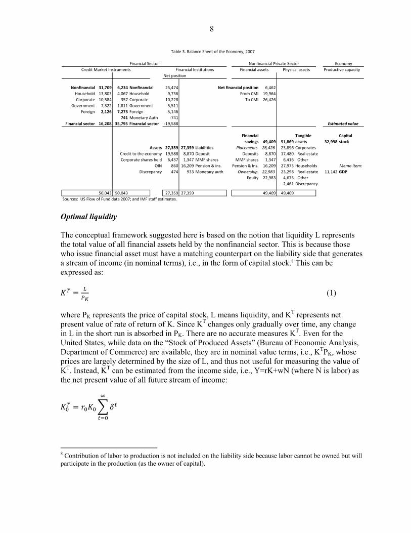
A financial asset is an instrument of a fiduciary agreement that in a broad sense is to serve the purpose of money. It is ultimately a claim on current or future goods and services and includes assets such as bank deposits, credit market instruments and equities.4 The rate of return on total financial assets in an economy is constrained by the rate of return on the physical capital stock plus the invisible assets captured by TFP of the economy as financial assets themselves do not generate income, but are claims on, including through ownership of, physical assets. Thus, the return on physical capital determines the boundary of returns on financial assets (excluding the value added generated from efficiency and risk management in the process of financial intermediation). In a similar vein, total value of financial assets should be broadly equal to the value of the physical assets (including the associated technology), which in turn is equal to the net present value of output generated by these physical assets (explained below). In other words, financial assets can be regarded as instruments that allow efficient use of capital within an economy without being constrained by ownership of capital (i.e., the traditional function of financial intermediation). The rationale for this definition is based on the fact that any issuer of a financial asset requires a counterpart liability, which, when traced back, ultimately has to be in current or future goods and services, or the capacity to generate them. To define liquidity, it is convenient to break the economy into nonfinancial and financial private sector. The following provides a balance sheet analysis of nonfinancial and financial private sector, and their connectedness (as an illustration, end-2007 US data is used).

2 Another motive behind this work was an attempt to refine financial programming to better capture the growing complexity of the financial sector.

3 The US data is used because the Fed’s comprehensive flow of fund data makes detailed illustration of the conceptual framework possible. Actual estimations are based on 8 Asian economies using constructed liquidity measures as illustrated using the US data. However, due to data constraints for several countries, liquidity measures are not as comprehensive as those shown for the US economy.

4 To the extent that equity is an asset representing an ownership interest, it is part of financial assets that can be liquidated and exchanged with goods and services.

6

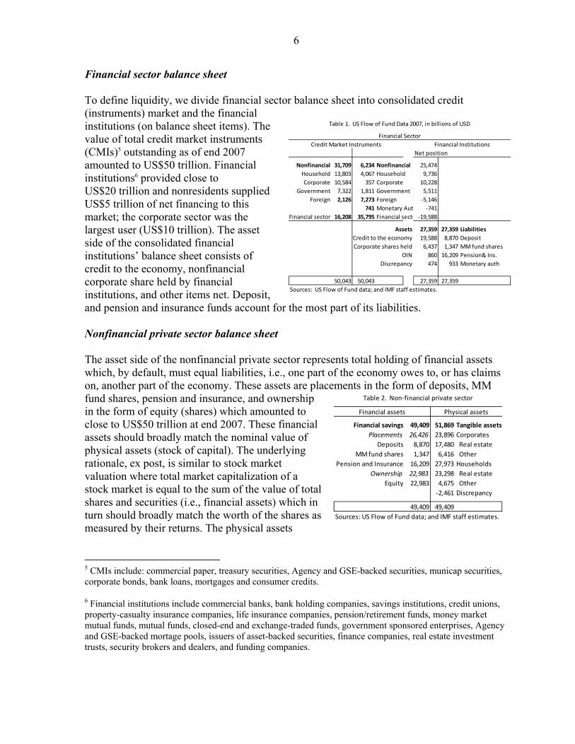
Financial sector balance sheet To define liquidity, we divide financial sector balance sheet into consolidated credit (instruments) market and the financial institutions (on balance sheet items). The value of total credit market instruments (CMIs)5 outstanding as of end 2007 amounted to US$50 trillion. Financial institutions6 provided close to US$20 trillion and nonresidents supplied US$5 trillion of net financing to this market; the corporate sector was the largest user (US$10 trillion). The asset side of the consolidated financial institutions’ balance sheet consists of credit to the economy, nonfinancial corporate share held by financial institutions, and other items net. Deposit, and pension and insurance funds account for the most part of its liabilities. Nonfinancial private sector balance sheet The asset side of the nonfinancial private sector represents total holding of financial assets which, by default, must equal liabilities, i.e., one part of the economy owes to, or has claims on, another part of the economy. These assets are placements in the form of deposits, MM fund shares, pension and insurance, and ownership in the form of equity (shares) which amounted to close to US$50 trillion at end 2007. These financial assets should broadly match the nominal value of physical assets (stock of capital). The underlying rationale, ex post, is similar to stock market valuation where total market capitalization of a stock market is equal to the sum of the value of total shares and securities (i.e., financial assets) which in turn should broadly match the worth of the shares as measured by their returns. The physical assets

5 CMIs include: commercial paper, treasury securities, Agency and GSE-backed securities, municap securities, corporate bonds, bank loans, mortgages and consumer credits.

6 Financial institutions include commercial banks, bank holding companies, savings institutions, credit unions, property-casualty insurance companies, life insurance companies, pension/retirement funds, money market mutual funds, mutual funds, closed-end and exchange-traded funds, government sponsored enterprises, Agency and GSE-backed mortage pools, issuers of asset-backed securities, finance companies, real estate investment trusts, security brokers and dealers, and funding companies.

Net position

Nonfinancial 31,709 6,234 Nonfinancial 25,474

Household 13,803 4,067 Household 9,736

Corporate 10,584 357 Corporate 10,228

Government 7,322 1,811 Government 5,511

Foreign 2,126 7,273 Foreign -5,146

741 Monetary Aut -741

Financial sector 16,208 35,795 Financial secto -19,588

Assets 27,359 27,359 Liabilities

Credit to the economy 19,588 8,870 Deposit

Corporate shares held 6,437 1,347 MM fund shares

OIN 860 16,209 Pension& Ins.

Discrepancy 474 933 Monetary auth

50,043 50,043 27,359 27,359

Sources: US Flow of Fund data; and IMF staff estimates.

Table 1. US Flow of Fund Data 2007, in billions of USD

Financial Sector

Credit Market Instruments Financial Institutions

Financial savings 49,409 51,869 Tangible assets

Placements 26,426 23,896 Corporates

Deposits 8,870 17,480 Real estate

MM fund shares 1,347 6,416 Other

Pension and Insurance 16,209 27,973 Households

Ownership 22,983 23,298 Real estate

Equity 22,983 4,675 Other

-2,461 Discrepancy

49,409 49,409

Sources: US Flow of Fund data; and IMF staff estimates.

Financial assets Physical assets

Table 2. Non-financial private sector

7

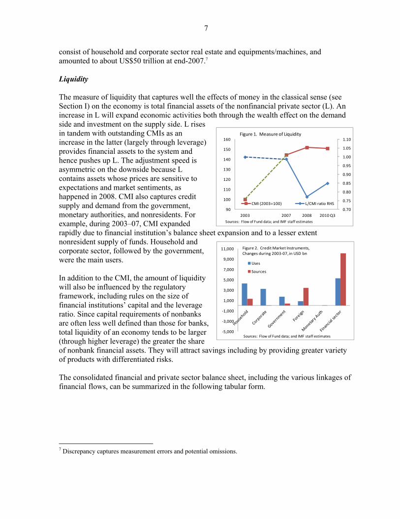
consist of household and corporate sector real estate and equipments/machines, and amounted to about US$50 trillion at end-2007.7 Liquidity The measure of liquidity that captures well the effects of money in the classical sense (see Section I) on the economy is total financial assets of the nonfinancial private sector (L). An increase in L will expand economic activities both through the wealth effect on the demand side and investment on the supply side. L rises in tandem with outstanding CMIs as an increase in the latter (largely through leverage) provides financial assets to the system and hence pushes up L. The adjustment speed is asymmetric on the downside because L contains assets whose prices are sensitive to expectations and market sentiments, as happened in 2008. CMI also captures credit supply and demand from the government, monetary authorities, and nonresidents. For example, during 2003–07, CMI expanded rapidly due to financial institution’s balance sheet expansion and to a lesser extent nonresident supply of funds. Household and corporate sector, followed by the government, were the main users. In addition to the CMI, the amount of liquidity will also be influenced by the regulatory framework, including rules on the size of financial institutions’ capital and the leverage ratio. Since capital requirements of nonbanks are often less well defined than those for banks, total liquidity of an economy tends to be larger (through higher leverage) the greater the share of nonbank financial assets. They will attract savings including by providing greater variety of products with differentiated risks. The consolidated financial and private sector balance sheet, including the various linkages of financial flows, can be summarized in the following tabular form.

7 Discrepancy captures measurement errors and potential omissions.

0.70

0.75

0.80

0.85

0.90

0.95

1.00

1.05

1.10

90

100

110

120

130

140

150

160

2003 2007 2008 2010 Q3

Figure 1. Measure of Liquidity

CMI (2003=100) L/CMI ratio RHS

Sources: Flow of Fund data; and IMF staff estimates

-5,000

-3,000

-1,000

1,000

3,000

5,000

7,000

9,000

11,000 Figure 2. Credit Market Instruments,Changes during 2003-07, in USD bn

Uses

Sources

Sources: Flow of Fund data; and IMF staff estimates

8

Optimal liquidity The conceptual framework suggested here is based on the notion that liquidity L represents the total value of all financial assets held by the nonfinancial sector. This is because those who issue financial asset must have a matching counterpart on the liability side that generates a stream of income (in nominal terms), i.e., in the form of capital stock.8 This can be expressed as:

  (1)

where PK represents the price of capital stock, L means liquidity, and KT represents net present value of rate of return of K. Since KT changes only gradually over time, any change in L in the short run is absorbed in PK. There are no accurate measures KT. Even for the United States, while data on the “Stock of Produced Assets” (Bureau of Economic Analysis, Department of Commerce) are available, they are in nominal value terms, i.e., KTPK, whose prices are largely determined by the size of L, and thus not useful for measuring the value of KT. Instead, KT can be estimated from the income side, i.e., Y=rK+wN (where N is labor) as the net present value of all future stream of income:

8 Contribution of labor to production is not included on the liability side because labor cannot be owned but will participate in the production (as the owner of capital).

Productive capacity

Net position

Nonfinancial 31,709 6,234 Nonfinancial 25,474 Net financial position 6,462

Household 13,803 4,067 Household 9,736 From CMI 19,964

Corporate 10,584 357 Corporate 10,228 To CMI 26,426

Government 7,322 1,811 Government 5,511

Foreign 2,126 7,273 Foreign -5,146

741 Monetary Auth -741

Financial sector 16,208 35,795 Financial sector -19,588

Financial

savings 49,409 51,869

Tangible

assets 32,998

Capital

stock

Assets 27,359 27,359 Liabilities Placements 26,426 23,896 Corporates

Credit to the economy 19,588 8,870 Deposit Deposits 8,870 17,480 Real estate

Corporate shares held 6,437 1,347 MMF shares MMF shares 1,347 6,416 Other

OIN 860 16,209 Pension & ins. Pension & Ins. 16,209 27,973 Households Memo Item:

Discrepancy 474 933 Monetary auth Ownership 22,983 23,298 Real estate 11,142 GDP

Equity 22,983 4,675 Other

-2,461 Discrepancy

50,043 50,043 27,359 27,359 49,409 49,409

Sources: US Flow of Fund data 2007; and IMF staff estimates.

Estimated value

Table 3. Balance Sheet of the Economy, 2007

Financial Sector Nonfinancial Private Sector Economy

Credit Market Instruments Financial Institutions Financial assets Physical assets

9

r0 is rate of return on capital at period zero and δ=1-ρ where ρ is rate of depreciation.9 This can be rewritten as:

11

or alternatively as:

(2)

where PG is GDP deflator.10 Nominal value of capital at time zero is equal to nominal GDP times capital income share of GDP, and multiplied by the scale factor obtained by the rate of depreciation. We define this as the optimal level of liquidity, Lo

* at t=0. Actual liquidity will likely move around the path of the optimal level of L and small divergences will not have any major impact on the economy. However, if the divergence becomes large and persistent, the adjustment could be abrupt with negative spillover to economic activities.11 For example, in the United States, the value of PGKT in 2007 is estimated at US$34 trillion. This calculation is based on the estimated value of the real stock of capital through the perpetual inventory method and adjusted for IT and communication capital and represents the average value during the 1990s. 12 It also assumes a rate of time series depreciation of 10 percent per year, and cross section depreciation of 3 percent. This estimated value of capital in 2007 is well below the total liquidity of US$50 trillion, i.e., . Eventually, the gap between what the economy owes to one part of itself and the ability to meet this obligation will have to be closed, and often through an abrupt adjustment. So why does the total outstanding amount of credit instruments, i.e., CMIs, matter? It matters because an increase in the amount of CMI raises the total financial asset, i.e., liquidity, held by the private sector, similar to the traditional money creation through the banking system. In

9 The rate of depreciation is the addition of time series depreciation (the loss of value of an asset over time) and cross section depreciation (the loss of value due to technological advances) as defined by P. Hill (1999).

10 To further refine this analysis, some cost parameter could be added to GDP deflator, e.g., backed out from Tobin’s Q, reflect the adjustment cost of capital.

11 This issue is not further pursued in this paper since the main purpose is to highlight the importance of quantity of liquidity on the real sector.

12 See Khatri and Lee (2001).

-3000

-1000

1000

3000

5000

7000

9000

1995 2000 2003 2007 2008 2010 Q3

Figure 3. Measure of Gap between Financial and

Physical Asset, In USD bn

Sources: Flow of Fund data; and IMF staff estimates

10

fact, the excess (i.e., value of financial assets held by the private sector over capital stock) peaked in 2007 at US$7.8 trillion. It was reduced to negative gap of US$2 trillion by 2010 largely through the fall of prices of equities held by the private sector. This compares with the total financial assets held by the nonfinancial private sector in 1995 of US$20 trillion, which was about US$1.7 trillion less than the estimated capital value. At the optimal level of liquidity, GDP deflator and price of capital stock should be equal, i.e.,

(3)

An increase in CMI, and hence L, has disproportionate impact on GDP deflator and on asset prices. It impacts GDP deflator PG through the traditional M GDP channel whereby the demand side is affected through the wealth effect, and the supply side by more credit (lower interest rate) and hence investment. However, the impact of L on asset price is much more direct and larger. This creates a gap between the face value of assets and what it can actually purchase in terms of goods and services. Moreover, it widens income disparity between those who depend on flows (annual income) and on stock (holding wealth). Under a steady state situation, GDP deflator should increase in tandem with the price of capital. If the latter increase faster than the former, liquidity (asset) expansion will exceed the actual capacity of the economy (liability) to meet the obligation underlying financial assets, i.e., liquidity.

III. TESTING FOR CAUSALITY BETWEEN LIQUIDITY AND PRICES

We test for the causality of liquidity on the price of capital, i.e., L impact on PK using panel data on 8 Asian economies, i.e., Australia, China, Japan, Korea, Indonesia, Malaysia, Philippines, and Thailand (i.e., ASEAN4+3, Australia). In other words, we test to see whether equation (1), i.e., holds. Multiplying (1) by PG/PK , we obtain

which at steady state (i.e.,, where there are no pressures for PG to diverge from PK),

, i.e., equation (3) above.13

The Gap is defined as:

(4)

13 The condition does not have to hold always even under L*. For example, in the case of a positive productivity shock, .

Interestrates

CMILiquidity

Price

of assets

CPI

Monetary policy

Instrument:policy rate

Figure 4. Disproportionalte Transmission of Monetary Policy

11

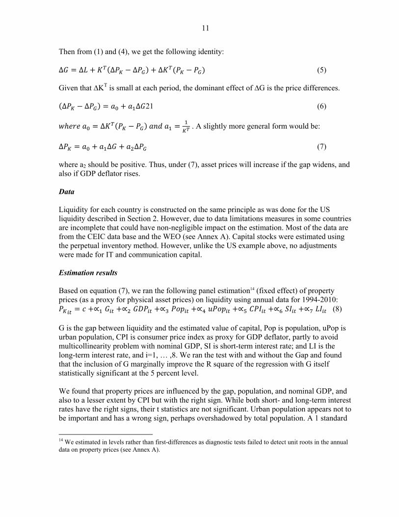
Then from (1) and (4), we get the following identity: ∆ ∆ ∆ ∆ ∆ (5) Given that ∆KT is small at each period, the dominant effect of ∆G is the price differences. ∆ ∆ ∆ 21 (6)

  ∆     . A slightly more general form would be:

∆ ∆ ∆ (7) where a2 should be positive. Thus, under (7), asset prices will increase if the gap widens, and also if GDP deflator rises. Data Liquidity for each country is constructed on the same principle as was done for the US liquidity described in Section 2. However, due to data limitations measures in some countries are incomplete that could have non-negligible impact on the estimation. Most of the data are from the CEIC data base and the WEO (see Annex A). Capital stocks were estimated using the perpetual inventory method. However, unlike the US example above, no adjustments were made for IT and communication capital. Estimation results Based on equation (7), we ran the following panel estimation14 (fixed effect) of property prices (as a proxy for physical asset prices) on liquidity using annual data for 1994-2010:

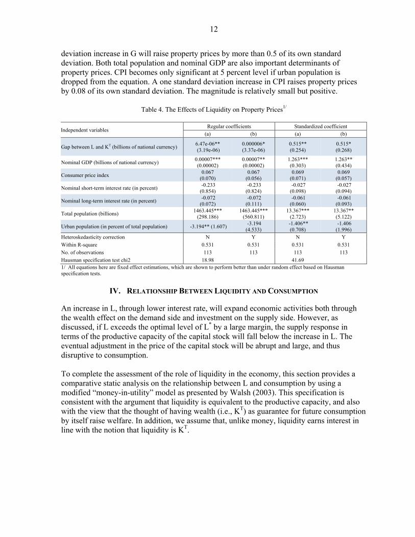
(8) G is the gap between liquidity and the estimated value of capital, Pop is population, uPop is urban population, CPI is consumer price index as proxy for GDP deflator, partly to avoid multicollinearity problem with nominal GDP, SI is short-term interest rate; and LI is the long-term interest rate, and i=1, … ,8. We ran the test with and without the Gap and found that the inclusion of G marginally improve the R square of the regression with G itself statistically significant at the 5 percent level. We found that property prices are influenced by the gap, population, and nominal GDP, and also to a lesser extent by CPI but with the right sign. While both short- and long-term interest rates have the right signs, their t statistics are not significant. Urban population appears not to be important and has a wrong sign, perhaps overshadowed by total population. A 1 standard

14 We estimated in levels rather than first-differences as diagnostic tests failed to detect unit roots in the annual data on property prices (see Annex A).

12

deviation increase in G will raise property prices by more than 0.5 of its own standard deviation. Both total population and nominal GDP are also important determinants of property prices. CPI becomes only significant at 5 percent level if urban population is dropped from the equation. A one standard deviation increase in CPI raises property prices by 0.08 of its own standard deviation. The magnitude is relatively small but positive.

Table 4. The Effects of Liquidity on Property Prices1/

Independent variables Regular coefficients Standardized coefficient

(a) (b) (a) (b)

Gap between L and KT (billions of national currency) 6.47e-06** (3.19e-06)

0.000006* (3.37e-06)

0.515** (0.254)

0.515* (0.268)

Nominal GDP (billions of national currency) 0.00007*** (0.00002)

0.00007** (0.00002)

1.263*** (0.303)

1.263** (0.434)

Consumer price index 0.067

(0.070) 0.067

(0.056) 0.069

(0.071) 0.069

(0.057)

Nominal short-term interest rate (in percent) -0.233 (0.854)

-0.233 (0.824)

-0.027 (0.098)

-0.027 (0.094)

Nominal long-term interest rate (in percent) -0.072 (0.072)

-0.072 (0.111)

-0.061 (0.060)

-0.061 (0.093)

Total population (billions) 1463.445***

(298.186) 1463.445***

(560.811) 13.367***

(2.723) 13.367** (5.122)

Urban population (in percent of total population) -3.194** (1.607) -3.194 (4.533)

-1.406** (0.708)

-1.406 (1.996)

Heteroskedasticity correction N Y N Y

Within R-square 0.531 0.531 0.531 0.531

No. of observations 113 113 113 113

Hausman specification test chi2 18.98 41.69 1/ All equations here are fixed effect estimations, which are shown to perform better than under random effect based on Hausman specification tests.

IV. RELATIONSHIP BETWEEN LIQUIDITY AND CONSUMPTION

An increase in L, through lower interest rate, will expand economic activities both through the wealth effect on the demand side and investment on the supply side. However, as discussed, if L exceeds the optimal level of L* by a large margin, the supply response in terms of the productive capacity of the capital stock will fall below the increase in L. The eventual adjustment in the price of the capital stock will be abrupt and large, and thus disruptive to consumption. To complete the assessment of the role of liquidity in the economy, this section provides a comparative static analysis on the relationship between L and consumption by using a modified “money-in-utility” model as presented by Walsh (2003). This specification is consistent with the argument that liquidity is equivalent to the productive capacity, and also with the view that the thought of having wealth (i.e., KT) as guarantee for future consumption by itself raise welfare. In addition, we assume that, unlike money, liquidity earns interest in line with the notion that liquidity is KT.

13

Model 15 Household’s preferences for consumption (c), labor (n), and holding liquidity (l) within given wealth W can be stated as:

),,(0

ttt

ti nlcuW

(9)

Subject to a budget constraint: (10)

or

where y is real output and c is real consumption, and l is L/P.16 We assume that the aggregate production function Y=F (A, k) is linear homogenous with constant returns to scale, A is total factor productivity, k=K/N, K is capital stock, and N is labor; 0)(lim,)(lim,0,0 0 kfkfff kkkkkkk . The value function, which is the present discounted value of household wealth, is defined as:

)}(),,(max{)( 1 ttttt VnlcuV (11)

subject to (10). This can be rewritten as:

tttt

ttttt lkc

likkf

)1(

)1()1()( 11

11 (12)

For illustrative purpose, the utility function is parameterized as follows. Households can be described as maximizing the expected present discounted value of utility:

111

11

1

0

itit

it

i

it

nl

cE (13)

Firms’ production function is defined as

ttt kAy and cost of firms is t

tttt P

Wkrq per labor

15 See Annex A for full exposition.

16 The specified utility function can be justified if one assumes asymmetry between creditors and debtors to the extent that the latter’s negative utility of holding debt is partly offset by utilizing the debt.

tttt

tttt lkc

liky

)1(

)1()1( 11

1

111 )1(

)1(

)1(

ttt

t

tttt kkc

lily

14

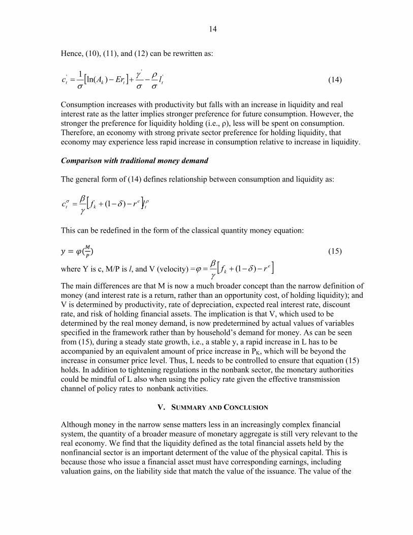
Hence, (10), (11), and (12) can be rewritten as:

''

' )ln(1

ttkt lErAc

(14)

Consumption increases with productivity but falls with an increase in liquidity and real interest rate as the latter implies stronger preference for future consumption. However, the stronger the preference for liquidity holding (i.e., ρ), less will be spent on consumption. Therefore, an economy with strong private sector preference for holding liquidity, that economy may experience less rapid increase in consumption relative to increase in liquidity. Comparison with traditional money demand The general form of (14) defines relationship between consumption and liquidity as:

te

kt lrfc )1(

This can be redefined in the form of the classical quantity money equation:

(15)

where Y is c, M/P is l, and V (velocity) = ek rf )1(

The main differences are that M is now a much broader concept than the narrow definition of money (and interest rate is a return, rather than an opportunity cost, of holding liquidity); and V is determined by productivity, rate of depreciation, expected real interest rate, discount rate, and risk of holding financial assets. The implication is that V, which used to be determined by the real money demand, is now predetermined by actual values of variables specified in the framework rather than by household’s demand for money. As can be seen from (15), during a steady state growth, i.e., a stable y, a rapid increase in L has to be accompanied by an equivalent amount of price increase in PK, which will be beyond the increase in consumer price level. Thus, L needs to be controlled to ensure that equation (15) holds. In addition to tightening regulations in the nonbank sector, the monetary authorities could be mindful of L also when using the policy rate given the effective transmission channel of policy rates to nonbank activities.

V. SUMMARY AND CONCLUSION

Although money in the narrow sense matters less in an increasingly complex financial system, the quantity of a broader measure of monetary aggregate is still very relevant to the real economy. We find that the liquidity defined as the total financial assets held by the nonfinancial sector is an important determent of the value of the physical capital. This is because those who issue a financial asset must have corresponding earnings, including valuation gains, on the liability side that match the value of the issuance. The value of the

15

earnings of a physical asset in turn is the real net present value of return of the capital stock, which depreciates over time, multiplied by the price of the capital stock. The optimal amount of liquidity is attained at the level where it equals the real earnings times the GDP deflator. This is because the nominal earnings (income flows) of capital by default are measured as a scale to nominal GDP (i.e., relevant because of purchasing power). A Gap is created if the amount of liquidity exceeds this optimal level, which will be reflected through a fall in the GDP deflator/price of capital ratio. In other words, if the Gap arises due to a rapid expansion in liquidity, this will push up the price level of the capital stock at a much faster pace than the GDP deflator. As a result, this gap will (i) lead to a boom and bust cycle if left unchecked, which is disruptive to the economy, and (ii) worsen income inequality by rewarding those with capital stock more than those who depend on flow of income. While it is true that interest rate transmission mechanism has become an effective monetary policy instrument aimed at controlling inflation, monetary aggregate is also still relevant to providing economic stability. By broadening the definition of money to include all financial assets held by the nonfinancial private sector, and then targeting the total to a level that is consistent with the optimal level liquidity as discussed in this paper, economic and price stability can be achieved. To achieve this desired outcome, monetary policy will have to use a combination of interest rate and monetary aggregate as the intermediate target.

16

REFERENCES

Bernanke, Ben S., 2006, “Monetary Aggregates and Monetary Policy at the Federal Reserve: A Historical Perspective,” remarks at the Fourth ECB Central Banking Conference on The Role of Money: Money and Monetary Policy in the Twenty-First Century, Frankfurt, November.

Borio, C., N. Kennedy, and S. D. Prowse, 1994, “Exploring Aggregate Asset Price

Fluctuations Across Counties: Measurement, Determinants, and Monetary Policy Implications,” BIS Economic Papers, No. 40.

Borio, C., and P. Lowe, 2002, “Asset Prices, Financial and Monetary Stability: Exploring the

Nexus,” BIS Working Paper No.114. Fisher, Irving, 1911, “The Purchasing Power of Money, its Determination and Relation to

Credit, Interest and Crises,” New and Revised Edition, ed. by Harry G. Brown (New York: Macmillan, 1922).

Gerdesmeier, Dieter, Hans-Eggert Reimers, and Barbara Roffia, 2009, “Asset Price

Misalignments and the Role of Money and Credit,” European Central Bank Working Paper No. 1068.

Helbling, T., and M. Terrones, 2003, “When Bubbles Burst,” in World Economic Outlook,

(Washington: International Monetary Fund). Hill, P., 1999, “Capital Stocks, Capital Services, and Depreciation,” paper presented at the

Third Meeting of the Canberra Group on Capital Stock Statistics, November 8–10, Washington, DC.

Keynes, John M., 1936, The General Theory of Employment, Interest Rates, and Money,

(Cambridge: Cambridge University Press). Kahn, George A., and Scott Benolkin, 2007, “The Role of Money in Monetary Policy: Why

do the Fed and ECB see it so differently?” Available via the Internet: http://www.kansascityfed.org/publicat/newsroom/2007pdfs/pr07-22.pdf.

Khatri, Y, and Il Houng Lee, 2001, “Information Technology and Productivity Growth in

Asia,” IMF Working Paper No. 03/15 (Washington: International Monetary Fund). Friedman, Milton, 1956, “The Quantity Theory of Money: A Restatement” in Studies in the

Quantity Theory of Money, ed. by M. Friedman. Walsh, Carl E., 2003, Monetary Theory and Policy, 2nd Edition (Cambridge, Massachusetts:

MIT Press).

17

Woodford, Michael, 2007, “How Important is Money in the Conduct of Monetary Policy?” Revised July 2007, paper presented at the Conference in Honor of Ernst Baltensperger, University of Bern, June.

18

Annex A. Sources of Data and Estimation Results 1. Data Liquidity Australia China Japan Indonesia Korea Malaysia Philippines Thailand Broad money

Yes Yes Yes Yes Yes Yes Yes Yes

Bond Yes Yes Yes Yes Yes Yes Yes Yes Insurance Yes Yes Yes Yes Yes Yes Social security

Yes

Equity Yes Yes Yes Yes Yes Yes Yes Yes

Sources: Australia: CEIC, Australian Securities Exchange, Reserve Bank of Australia, World Federation of Exchanges China: CEIC, People’s Bank of China Japan: CEIC Indonesia: CEIC, Jakarta Stock Exchange, Surabaya Stock Exchange, Bank Indonesia Korea: CEIC, Bank of Korea Malaysia: CEIC Philippines: CEIC Thailand: CEIC Adjustments are made:

Bonds and insurance funds held by banks to address double counting. Pension funds were not added as most of the amount was held in other forms already

captured in the total, i.e., bank deposits, bonds, and equities. Capital stock Capital stocks were estimated using the perpetual inventory method. A depreciation rate of 12 percent was used for all countries (10 percent for time series depreciation and 2 percent for cross section depreciation). Marginal variations to the latter do not affect the estimated results. Data sources are from the CEIC, World Economic Outlook (IMF), and the International Labor Office (for wages). We show below the estimated results with and without urban population and for both imposed, and not imposed, correction for Heteroskedasticity.

19

2. Estimation Unit root tests Fisher-type Unit root tests (based on augmented Dickey-Fuller test) were carried out on the endogenous as well as exogenous variables. The null hypothesis was existence of a unit root. Number of panels = 8 Avg. number of periods = 14.13 ADF regressions: 1 lag Property price Gap CPI ST interest rate LT interest rate Inverse Chi-squared (16)

22.629 (0.124) 4.086 (0.998) 69.586 (0.000) 37.134 (0.002) 30.556 (0.015)

Inverse normal -1.115 (0.132) 2.742 (0.996) -3.536 (0.000) -1.882 (0.029) -1.744 (0.040) Inverse logit (39) -1.042 (0.151) 2.849 (0.996) -6.121 (0.000) -2.591 (0.006) -2.096 (0.020)

( ) are p-values Because we could not reject the null hypothesis on Gap, the same regressions were run on first difference. However, we could not generate any meaningful information with R-square below 0.1 and insignificant t statistics on most variables. Panel regression with and without the Gap A panel estimation (fixed effect) results below show that inclusion of the Gap improves not only the fit but also marginally the t statistics for some variables that should be, a priori, included in the regression. Moreover, the t-statistic on the Gap itself is significant. Independent variables Without Gap With Gap Gap

6.47e-06**

(2.03) CPI 0.0654

(0.93) 0.0673 (0.97)

GDP 0.0000*** (5.67)

0.0000*** (4.17)

ST interest rate -0.7706 (-0.93)

-0.2331 (-0.27)

LT interest rate -0.0666 (-0.91)

-0.0722 (-1.00)

Population 1404.23*** (4.66)

1463.44*** (4.91)

Urban population -2.8694 (-1.77)

-3.1939** (-1.99)

constant -44.043 (-0.70)

-48.354 (-0.78)

Within R-sq 0.5112 0.5308 No. of observations 113 113

20

Annex B. Relationship Liquidity and Demand Household’s preferences for consumption (c), labor (n), and holding liquidity (l) within given wealth W can be stated as:

),,(0

ttt

ti nlcuW

(1.1)

Subject to a budget constraint:

t

ttt

t

tttt P

Lkc

P

Liky

11

1

)1()1( (1.2)

or similarly:

where y is real output and c is real consumption, and l is L/P. Assuming that the aggregate production function Y=F (A, k) is linear homogenous with constant returns to scale, A is total factor productivity, k=K/N, K is capital stock, and N is labor. Further assume that 0)(lim,)(lim,0,0 0 kfkfff kkkkkkk

The value function, which is the present discounted value of household wealth is defined as:

)}(),,(max{)( 1 ttttt VnlcuV (1.3)

subject to (1.2). This can be rewritten as.

tttt

ttttt lkc

likkf

)1(

)1()1()( 11

11 (1.4)

or

)1(

)1())(1()(

t

ttttttttt

lilclcf

(1.5)

The first order conditions are17:

0)()1(

)()1()1((

1

1

tkC

tk

Vfu

VfC

u

C

V

(1.6)

17 See P. Geraats (..) for solving the value function using the Bellman equation.

tttt

tttt lkc

liky

)1(

)1()1( 11

1

21

0)()1(

)1()1(

)()1(

)1()1()1((

1

11

tt

tkL

tt

tk

Vi

fu

Vi

fL

u

L

V

(1.7)

The envelope theorem implies:

),,()( 111111 tttct nlcuV

Hence,

))1((

))1((

1

1

kC

C

CkC

fu

u

ufu

The intertemporal consumption decision is influenced by productivity and capital stock adjusted for depreciation, and discounted marginal utility of future consumption. The intuition is that as income rises from productivity gains, more can be consumed without loss of future consumption. Also:

C

C

C

L

CCL

CkL

u

uEr

u

u

uEruu

uErfu

1

1

1

)(1

)(

))1((

For illustrative purpose, the utility function is parameterized as follows: Households can be described as maximizing the expected present discounted value of utility:18

111

11

1

0

itit

it

i

it

nl

cE (2.1)

Then FOCs from (1.6) are:

1))1(( tkt Ecfc (2.2)

Intertemporal consumption preference is determined by marginal product of capital and the rate of depreciation. An increase in MP of capital or a fall in the depreciation rate leads to an increase in future consumption. Likewise, from (1.7),

18 Modified from Walsh (5.46) on page 232

22

11

1)1( t

t

tkt Ec

E

ifl (2.3)

))1((1

1)1(

1

k

t

t

tkt f

c

E

ifl

Preference for holding money increases as real interest rate (deflated by expected inflation) rises, or declines when marginal product of capital increases. Consumption decision is further influenced by γ (some measure of risk in financial instrument).

tk

e

t lf

rc

))1((

11

(2.4)

Firms’ production function is defined as:

ttt kZy

Cost of firms is t

tttt P

Wkrq per labor

Then the firm’s problem becomes solving for

)(min ttttttt

t

kkAykr

P

W

Hence, the FOC is

)( tttttt wqnAr (2.5)

k=K/N, and w=W/P Hence, (2.2), (2.3), and (2.4) can be rewritten as:

''

' )ln(1

ttkt lErAc

As productivity increases relative to the cost of capital, less liquidity is held since higher income ensures future consumption is not compromised.