CHE Research Paper 130

Optimal Hospital Payment Rules Under Rationing By Random Waiting

Hugh Gravelle, Fred Schroyen

Optimal hospital payment rules under rationing by random waiting

1Hugh Gravelle 2Fred Schroyen

1Centre for Health Economics, University of York, York, UK

2Department of Economics, Norwegian School of Economics, Bergen, Norway May 2016

Background to series

CHE Discussion Papers (DPs) began publication in 1983 as a means of making current research material more widely available to health economists and other potential users. So as to speed up the dissemination process, papers were originally published by CHE and distributed by post to a worldwide readership. The CHE Research Paper series takes over that function and provides access to current research output via web-based publication, although hard copy will continue to be available (but subject to charge). Acknowledgements

We received helpful comments from Gjermund Grimsby, Philippe Bontem and other participants at the 2015 Annual Conference of the Norwegian Economic Association (Bergen) and at the 2015 European Health Economics Workshop (Toulouse). Further copies

Copies of this paper are freely available to download from the CHE website www.york.ac.uk/che/publications/ Access to downloaded material is provided on the understanding that it is intended for personal use. Copies of downloaded papers may be distributed to third-parties subject to the proviso that the CHE publication source is properly acknowledged and that such distribution is not subject to any payment. Printed copies are available on request at a charge of £5.00 per copy. Please contact the CHE Publications Office, email che-pub@york.ac.uk, telephone 01904 321405 for further details. Centre for Health Economics Alcuin College University of York York, UK www.york.ac.uk/che © Hugh Gravelle, Fred Schroyen

Optimal hospital payment rules under rationing by randomwaiting¤

Hugh Gravelley Fred Schroyenz

26 April 2016

Abstract We derive optimal rules for paying hospitals in a public health care systemin which providers can choose quality and random patient demand is rationed by waitingtime. Since waiting time imposes real costs on patients hospital payment rules should takeaccount of their e¤ect on waiting time as well as on quality and the number of patientstreated. We develop a general stochastic model of rationing by waiting and use it toderive welfare maximising payment to hospitals linked to output, expected waiting times,quality, hospital capacity and length of stay. We show that, although prospective outputpricing gives hospitals an incentive to attract patients by raising quality and reducingwaiting times, it must be supplemented by prices attached to other hospital decisionsand outcomes except under very strong assumptions about the welfare function, patientpreferences, and whether patients lose income whilst waiting.

Keywords: Rationing. Waiting times. Queues. Prospective payment. Hospitals.

JEL code: I11, I13, I18, L51, D81

¤We received helpful comments from Gjermund Grimsby, Philippe Bontem and other participants atthe 2015 Annual Conference of the Norwegian Economic Association (Bergen) and at the 2015 EuropeanHealth Economics Workshop (Toulouse).

yCentre for Health Economics, University of York. Email: hugh.gravelle@york.ac.uk.zDepartment of Economics, Norwegian School of Economics. Email: fred.schroyen@nhh.no.

1 Introduction

Public hospital systems, like those in Scandinavia, the UK, and other OECD countries,are mainly …nanced through general taxation or compulsory social insurance. Patientsface zero or very low money prices and consequently non-emergency treatment is rationedby waiting time (Cullis et al., 2000; Siciliani and Iversen, 2012). Such waiting times areoften long and a source of concern to both patients and policy makers.1 There are alsoconsiderable variations in quality and costs amongst hospitals. Hospitals in these systemsare increasingly paid prospectively for each case treated (Paris et al., 2010) and in somecountries there are attempts to improve hospital quality by linking payment directly toquality as well as to output (Jha et al., 2012; Sutton et al., 2012).

In this paper we derive optimal rules for paying hospitals in a public health care systemin which patient demand is rationed by waiting time and hospitals can choose quality andmake supply decisions that change the distribution of waiting times facing patients.

Although both quality and waiting time a¤ect patient demand and both can be in-‡uenced by hospital decisions, quality is determined solely by hospital decisions whereaswaiting time is determined by both patient demand and hospital supply. Waiting time isnot just another type of quality and cannot be treated as just another quality dimensionwhen analysing payment rules: it is necessary to allow for the fact that waiting time isalso a rationing device which equates patient demand and hospital supply and does so byimposing costs on patients which are not o¤set by gains to providers. Payment rules haveto be designed in the light of their e¤ect on these rationing costs as well as on hospitalquality and the number of patients treated.

The literature on the welfare implications of alternative hospital payment systems isreviewed in Chalkley and Malcomson (2000). The aim of the payment system is to inducewelfare maximising hospital behaviour: treatment of an optimal number of patients withoptimal quality at minimum cost. In this literature it is assumed that payment cannot belinked directly to unveri…able or unobserved quality and cost reducing e¤ort. Policy mak-ers are restricted to setting a price for output and to reimbursing hospitals for their costs.In Ellis and McGuire (1986) the number of patients requiring treatment is not a¤ected byhospital decisions and …rst best quality and cost reducing e¤ort are not achievable. Theyshow that the second best welfare maximising reimbursement rule combines a prospec-tive price per patient treated and partial reimbursement of hospital costs. With only aprospective price and an exogenously determined number of patients requiring treatmentthe hospital will skimp on quality, unless it is perfectly altruistic, because quality is costlyand has no e¤ect on its revenue. Partial reimbursement of costs reduces the marginal costof quality and so induces the hospital to increase quality. But partial cost reimbursementalso reduces the incentive for cost reducing e¤ort so that the second best mixed reim-bursement scheme trades o¤ quality and cost reducing e¤ort. Despite having two policytargets (quality and cost reducing e¤ort) and two policy instruments the …rst best is notachievable because, with a …xed number of patients, the prospective price is equivalent toa lump sum payment with no incentive properties: the only instrument which a¤ects the

1For example, the median waiting time from being placed on the waiting list for hip replacement totreatment in 2011 was 108 days in Australia, 113 in Finland, 87 in Portugal, and 82 in England (Sicilianiet al., 2014). See Cullis et al. (2000), Iversen and Siciliani (2011) and Siciliani and Iversen (2012) forsurveys of the health economics waiting time literature.

1

hospital quality decision is cost reimbursement.Chalkley and Malcomson (1998) consider payments regimes when patient demand

varies with quality.2 They show that, if (a) there is only one dimension of quality and(b) it is optimal to treat all patients who demand care at the optimal quality, then …rstbest quality and output can be achieved at minimum cost with a single instrument: aprospective output price. Because higher quality attracts more patients, thus increasingrevenue, hospitals respond to a higher price by increasing quality. It is thus possible to setthe price so that the hospital chooses the optimal quality and this results in the optimalnumber of patients being treated. And with no cost reimbursement the hospital bears allthe costs of producing care and so has the appropriate incentive for cost reducing e¤ort.Remarkably, this result does not depend on the policy maker and patients having the samevaluation of quality and the bene…ts of treatment. It is not even necessary that patientscorrectly perceive quality when demanding care, only that their demand is increasing inquality as perceived by the policy maker. But Chalkley and Malcomson (1998) also showthat if quality is multi-dimensional, the …rst best is implementable via the output priceonly if the policy maker and patients have the same relative marginal valuations of thedi¤erent quality dimensions.

The insights from this literature are obtained from models which do not take account ofrationing by waiting time which is a salient feature of many public health care systems. It isimplicitly assumed that demand is not a¤ected by waiting time.3 But there is considerableevidence that waiting times do a¤ect demand for elective care. Higher waiting times leadpatients to switch within the public sector to hospitals with lower waiting times (Sivey,2012), to opt for private hospitals (Besley et al. 1999, Aarbu, 2010) or to forgo careentirely (Martin and Smith, 1999; Gravelle et al., 2002; Windmeijer et al., 2005).

Following Lindsay and Feigenbaum (1984) most formal models of rationing by waitingin health care assume that demand and supply, and hence waiting time, are deterministic.4

The certain waiting time adjusts, like the money price in standard markets, to ensure thatthe certain demand equals the certain supply. Such deterministic waiting time modelsare useful for some purposes but are ‡awed as a basis for modelling hospital behaviourand the welfare implications of regulation and pricing regimes. With a positive waitingtime a hospital can reduce quality whilst holding supply constant. Waiting time will fallto equate demand and the unchanged supply and so hospital revenue is unchanged. Sincecost is reduced because quality is lower, pro…t is increased. Hence, a pro…t maximisinghospital whose revenue varies with the volume of patients treated will never choose to haveboth positive waiting time and positive quality. Thus in deterministic models of rationingby waiting, the only way to explain the coexistence of positive waiting times and positivequality, is by assuming su¢ciently great direct provider concern with quality.

In stochastic queueing models waiting times are determined by the random demandfor treatment (conditional on quality) and random length of treatment. Waiting times are

2The Ellis and McGuire (1986) setting is akin to emergency treatment and in Chalkley and Malcomson(1998) it is akin to elective treatment where patients choose amongst alternatives (including no treatment).

3When demand exceeds supply Chalkley and Malcomson (1998) assume that there is perfect rationing(all patients treated have higher bene…ts that those who are not selected for treatment) or random rationing.But neither method of rationing is assumed to impose any direct costs on patients (other than not beingtreated if not selected) and patient demand is assumed una¤ected the probability of treatment.

4See, for example, Marchand and Schroyen (2005), and Gravelle and Siciliani (2008).

2

therefore also random. In equilibrium there is a steady state distribution of waiting timesdetermining the mean waiting time and the mean number of patients treated per period.The mean number treated is equal to the mean demand and less than the capacity of thehospital. The mean waiting time is positive since only an in…nitely large service capacitycan result in all patients having a zero realised waiting time. A reduction in quality willreduce costs but it will also reduce expected demand and thus expected output and revenueand so may not increase expected pro…t. Thus the equilibrium of the system will alwayshave positive expected waiting time and may, if quality is not too costly, have a positivequality.

Two papers in the health economics literature have considered stochastic waiting timemodels with demand depending on the distribution of waiting times.5 In Goddard et al.(1995) it is assumed that a patient observes the length of the waiting list before decidingwhether to join the list or not. The resulting complicated expressions for the steady stateprobabilities on the number of people in the system and expected waiting time are usedto derive comparative static predictions about the e¤ects of patient income and the priceof private care. Iversen and Lurås (2002) use a much simpler queueing model to examinecompetition between GPs via their choice of quality and expected waiting time.

Because we use our model of rationing with random waits for normative rather thanpositive analysis we derive demand functions for treatment from patient preferences overincome, quality and waiting times, rather than making plausible but ad hoc assumptionsabout the demand functions. We derive a welfare function based on these preferences toexamine policy options. Like Iversen and Lurås (2002) we take an ex ante, or rationalexpectations, approach, though we have a much more general speci…cation of the queueingmodel and of individual preferences.6 In the rational expectations equilibrium individualsdecide whether to seek public treatment on the basis of an anticipated waiting time distri-bution and their decisions generate the anticipated distribution. By contrast to Goddardet al. (1995), this approach has the advantage of yielding an analytically tractable equi-librium steady state distribution of waiting times for the public system which can be usedto examine the welfare properties of payment schemes.7

We derive …rst and second-best payment schemes for a public hospital taking intoaccount their e¤ects on the hospital’s choice of quality, the number of beds and its servicerate, and their impacts on the equilibrium waiting time distribution. In the …rst best,when a prospective price is combined with payments related to any two of quality, beds,and service rate, the …rst best price per patient treated is less than the marginal social

5There are stochastic waiting time models of hospitals in the operations research literature (see, e.g.,Worthington (1987, 1991) and the survey by Fomundam and Herrmann (2007)). But none of these allowfor balking, i.e., for patient decisions to join the waiting list being a¤ected by the distribution of waitingtimes.

Some of the queuing literature does consider endogenous arrival processes or balking (Hassin and Haviv,2003). Analyses of pricing have focussed on the use of user charges to in‡uence demand and curb congestion,rather than on provider prices to encourage supply and quality. For economic analyses of user charges instochastic queueing models see Edelson and Hildenbrand (1975) and Naor (1969).

6For example, we allow demand to depend on the distribution of waiting times not just on the meanwaiting time.

7The assumption also explains the purchase of supplementary insurance against the cost of privatetreatment by individuals before they fall ill. This decision must be made ex ante and so be based onunconditional expectations about the distribution waiting times, not the distribution conditional on thenumber waiting at the date the individual falls ill.

3

bene…t per additional patient. This di¤erence is larger the stronger the hospital’s degreeof altruism, the greater the marginal cost of public funds, and the greater is the e¤ect ofwaiting lists and waiting times on lost earnings due to waiting for care. With a prospectiveprice and one other instrument the optimal second best price per patient treated is higherthan the …rst best price to compensate for the fact that only one of the hospital decisions(quality, service rate, number of beds) is directly incentivised. Only if the welfare functionrespects patient preferences over waiting time and quality, all patients are willing to tradeo¤ waiting time and quality at the same rate, and if there are no lost earnings from waitingfor treatment, can a prospective output price yield the …rst best quality and service ratesin the absence of other policy instruments.

In the Section 2 we describe the stochastic queueing process and patient choices be-tween public and private treatment, examine the e¤ects of hospital choice of quality andsupply decisions on the equilibrium demand and waiting time distribution, and set out thewelfare function. In Section 3 we derive the …rst best hospital …nancing scheme when theregulator has a su¢cient set of instruments. In Section 4, we limit this set and derive anddiscuss second and third best pricing rules. Section 5 compares stochastic and determin-istic waiting time models and shows that the deterministic speci…cation is unsatisfactoryas a model of hospital behaviour and hence as a the basis for a welfare analysis of optimalhospital payment systems. Section 6 concludes.

2 Model

2.1 Queueing model

We use a general model of the queueing process which includes some of the standardstochastic queueing models as special cases.8 However, unlike most queueing modelswe allow for the fact that demand (the arrival process) depends on the distribution ofwaiting times. Our focus is on obtaining a tractable analytical model of the resultingmarket equilibrium as a basis for deriving …rst and second-best payment schemes forpublic hospitals.

We assume that patients require elective treatment for a non-epidemic condition withprobability ¾. All patients have the same severity and health gain from treatment andthere is no prioritisation of patients who are treated in order of arrival on the waitinglist: the queue discipline is “…rst come, …rst served”. The mean rate of arrivals (patientsjoining the waiting list) per unit of time is ¸.

The hospital has k beds allowing it to treat k patients simultaneously. A patient’slength of stay once admitted is uncertain though the hospital can in‡uence it by varyingsta¢ng levels, theatre hours, and better coordination between departments. We sum-marise these supply decisions by ¹. Both k and ¹ will a¤ect the distribution of the lengthof time a patient waits on the list to be treated. ¹ will also e¤ect the distribution of lengthof stay for patients when admitted. Note that although for de…niteness we interpret k,¹as hospital decisions on beds and service rate they could be any hospital decisions shiftingthe distribution of waiting times.

8See Taylor and Karlin (1998, ch 9) or Gross et al. (2008, ch 2) for an introduction to queueing theory.

4

Because the arrival rate and length of stay are random, the time between being placedon the waiting list and admission to the hospital is also random. We assume that thestochastic processes governing additions to the list and length of stay imply that thetotal time w between referral to the hospital and completed treatment has a steady statedistribution function

H(w;¸; k; ¹), H¸ < 0;Hs > 0 (s = k; ¹): (1)

Thus increases in ¸ and reductions in k and ¹ produce …rst degree stochastic dominatingchanges in the distribution of waiting times, implying that the mean wait ¹w is increasingin the referral rate and decreasing in (k; ¹):

¹w =

Z 1

0wdH(w;¸; k; ¹) = ¹w(¸; k; ¹); ¹w¸ > 0; ¹ws < 0 (s = k; ¹): (2)

More importantly for our purposes, (1) implies that under the assumption that patientsprefer shorter waiting times, increases in ¸ and reductions in k or ¹ reduce the expectedutility of patients who decide to join the queue.

Table 1. Symbols and de…nitionsSymbol De…nition¾ probability of ill health¸ demand for public hospital (referral rate)¹; k public hospital supply decisions: service rate, number of bedsw; ¹w random, mean wait for public hospitalH(w;¸; k; ¹) waiting time distribution functionq quality in public hospitaly incomeF (y) income distribution functionu(y; q;w) utility if ill and treatment in public hospital after wait of w¹u(y; q; ¸; k; ¹) expected utility if ill and treatment in public hospitaluN (y) utility if not illv = ¾¹u+ (1¡ ¾)uN expected utility if treatment in public hospital when illvo(y ¡ °) expected utility with private insurance at premium °y threshold income: choice of public hospital if y · yB(q; ¸; k; ¹) aggregate patient welfarecH(q; ¸; k; ¹) public hospital expected costcI(q; ¸; k; ¹) expected total earnings loss due to waiting

Our results hold for all queuing systems which yield a waiting time distribution sat-isfying (1). One speci…c, and relatively straightforward, example is the M=M=k system9

in which the number of arrivals has a Poisson distribution with mean rate ¸, the lengthof stay has a negative exponential distribution with parameter ¹, and there are k servers(beds), with ¸ < k¹, so that the mean number of patients joining the waiting list is lessthan the mean number who are treated per unit of time. When k¹ exceeds the arrival

9M=M=k is the Kendall notation for a queueing system with Markov (memoryless) arrivals, Markovservice time and k servers.

5

rate ¸, there is a steady state for the queueing system such that the probabilities for agiven number of patients in the system (either waiting or being treated) are well-de…ned.From these, one can derive the probability of a patient being admitted without waiting,¼0(¸; k; ¹) (¼0¸ < 0, ¼0k > 0, ¼0¹ > 0) as well as the distribution for the waiting timewhen all beds are occupied. The distribution of the total waiting time (time on the listplus and time under treatment) is the convolution of two negative exponential distribu-tions and the mean wait is ¹w(¸; k; ¹) = 1

¹ + 1¡¼0k¹¡¸ . In the simple but instructive M=M=1

system the expected wait is ¹w(¸; ¹) = 1¹¡¸ . In the Appendix (Theorem A.1) we prove

that the M=M=k system has a distribution of waiting times satisfying (1).

2.2 Patients

A compulsory public health insurance system covers the costs of treatment in the publichospital. Income y per unit of time is distributed over [ymin; ymax] with distribution func-tion F (y). We assume that a patient waiting for treatment is unable to work but is fullyreimbursed by the social insurance system for foregone earnings of w ¢ y.10

Utility when ill and treated in the public hospital with quality q after a time w is

u = u(y; q;w); uy > 0; uq > 0; uw < 0:

u(¢) is a cardinal function which is increasing and concave in y and q and decreasing inw.11 We assume usually that there is a single dimension of quality but also consider theimplications of multiple quality dimensions. We normalize the quality variable so that theminimum quality is q = 0. Quality q re‡ects aspects of the hospital stay and treatmentthat alter utility but do not a¤ect length of stay. Examples might be the extent to whichpatients receive adequate pain management, are informed about the diagnosis, treatedwith respect by sta¤, and aspects of hotel services, such as privacy, visiting hours, andquality of food. The adoption of minimally invasive surgery techniques, nursing intensityor e¤ective hygiene which reduce the risk of acquiring hospital infections, are interpretedas e¤orts to reduce average length of stay and are captured by the treatment intensity ¹.

Waiting time in the public hospital is uncertain and expected utility when ill for apatient who decides not to take out private health care insurance and to be treated in thepublic hospital is

¹u(y; q; ¸; k; ¹) =

Zu(y; q;w)dH(w;¸; k; ¹); ¹u¸ < 0; ¹us > 0 (s = k; ¹):

The …rst order stochastic dominance properties of H and the assumption that patientsdislike waiting (uw < 0) imply that expected utility is decreasing in the arrival rate andincreasing in k and ¹.12

10Allowing the proportion of income lost whilst waiting to be less than one or to vary with income orto be jointly distributed with income would not change the results substantively.

11 In general, patients may distinguish between time spent on the waiting list and time spent in thehospital til discharge. We ignore this distinction because it would unnecessarily complicate the modelwithout a¤ecting its main results.

12 In their seminal paper, Lindsay and Feigenbaum (1984) assume that the e¤ect of waiting time iscaptured by exponential discounting: u(y; q)e¡Áw. With these preferences and uncertain w expectedutility is u(y; q)Ee¡Áw = u(y; q)JH(¡Á), where JH(¡Á) is the moment generating function for distribution

6

We sometimes consider two benchmark cases of patient preferences over public treat-ment. In the …rst case preferences are quasi-separable (QS) so that the marginal rate ofsubstitution between quality and waiting time is independent of income. Equivalently,the marginal rates of substitution between any pair of q; ¸; ¹; k are independent of income

¹u =

Z[a1(y) + a2(y)r(q;w)]dH(w;¸; k; ¹) = a1(y) + a2(y)R(q; ¸; k; ¹): (3)

with R(q; ¸; k; ¹)def=Rr(q; w)]dH(w;¸; k; ¹).

In the second special case (LN preferences) u is linear in w so that citizens only careabout the expected wait:

¹u =

Z[t1(y; q) + t2(y; q)w]dH(w;¸; k; ¹) = t1(y; q) + t2(y; q) ¹w(¸; k; ¹): (4)

With LN preferences the marginal rates of substitution amongst ¸; ¹; k are independentof income and quality.

Utility when in good health and not requiring hospital treatment uN(y) is an increas-ing concave function of income with uN (y) > u(y; q;w) (all y; q;w), so that immediatetreatment never makes a patient better o¤ than if healthy. Expected utility from nottaking out private health care insurance and being treated in the public hospital when illis

v(y; q; ¸; k; ¹)def= ¾¹u(y; q; ¸; k; ¹) + (1¡ ¾)uN (y); vy > 0; v¸ < 0; vz > 0 (z = q; k; ¹):

There is also a private hospital sector which provides care with a low certain wait wo

and higher quality qo than the public hospital. Individuals who know they will preferto use the private sector when ill buy full cover supplementary private insurance at anactuarially fair price °. Thus their utility when ill is uo = u(y ¡ °; qo; wo) = uo(y ¡ °)and utility when in good health is uN(y ¡ °). Expected utility from taking out privateinsurance and being treated in the private hospital is

vo(y ¡ °)def= ¾uo(y ¡ °) + (1¡ ¾)uN (y ¡ °):

We assume that vy(y; q; ¸; k; ¹) < voy(y¡ °), which holds if there is declining marginalutility of income, weak Edgeworth complementarity between income and quality of treat-ment (uyq ¸ 0) and uyw · 0. Hence there is a threshold income level y (assumed to be inthe interior of [ymin; ymax]) de…ned by

v(y; q; ¸; k; ¹)¡ vo(y ¡ °) = 0; (5)

such that all individuals with y · y choose the option of no private insurance and treatment

H(w). This has the analytical advantage of yielding tractable expressions for expected utility with somedistributions. For example, in the M=M=k system w has a negative exponential distribution and JH(¡Á) =k¹¡¸+Á¼0k¹¡¸+Á . However, the utility function is convex in w implying that a mean preserving spread in the

distribution of w would increase expected utility: the patient would be better o¤ with a riskier waitingtime distribution.

7

in the public hospital when ill. The threshold income y(q; ¸; k; ¹) has derivatives

yz(q; ¸; k; ¹) = ¡ vz(y; q; ¸; k; ¹)

vy(y; q; ¸; k; ¹)¡ voy(y ¡ °)> 0; (z = q; k; ¹) (6)

y¸(q; ¸; k; ¹) = ¡ v¸(y; q; ¸; k; ¹)

vy(y; q; ¸; k; ¹)¡ voy(y ¡ °)< 0: (7)

2.3 Rational expectations equilibrium

Since individuals fall ill at a rate ¾ and choose the public hospital if and only if theyhave y · y(q; ¸; k; ¹), they join the waiting list at the rate ¾F (y(q; ¸; k; ¹)). Hence theequilibrium arrival rate (patient demand for public hospital care), ¸(q; k; ¹), is implicitlyde…ned by

¸¡ ¾F (y(q; ¸; k; ¹)) = 0:

This embodies the rational expectations assumption: the distribution H(w;¸; k; ¹) uponwhich decisions about joining the waiting list for the public hospital are based coincideswith the distribution H(w;¸(q; k; ¹); k; ¹) that these decisions give rise to. Demand isincreasing in quality and supply since both increase the utility of the marginal patient:

¸z(q; k; ¹) =¾f(y)yz

1¡ ¾f(y)y¸> 0; z = q; k; ¹: (8)

We use e to denote equilibrium values of variables and functions. At the equilibriumthe threshold income level depends on hospital quality and supply decisions

ye(q; k; ¹) = y(q; ¸(q; k; ¹); k; ¹);

with

yez = yz + y¸¸z = yz + y¸¾f(y)yz

1¡ ¾f(y)y¸=

yz1¡ ¾f(y)y¸

2 (0; yz); (z = q; k; ¹): (9)

Using these results we have

Lemma 1 Hospital attributes z; x (z; x = q; k; ¹, z 6= x) have the same relative marginale¤ects on demand, threshold income and expected utility :

¸z¸x

=byz(q; ¸(q; k; ¹); k; ¹)byx(q; ¸(q; k; ¹); k; ¹)

=byez(q; k; ¹)byex(q; k; ¹)

=vez(by; q; k; ¹)vex(by; q; k; ¹)

=vz(by; ¸(q; k; ¹); q; k; ¹)vx(by; ¸(q; k; ¹); q; k; ¹)

: (10)

If utility is linear in the waiting time then it also true that

vzvx

=wz

wx(z; x = ¸; k; ¹): (11)

The direct e¤ects of q and k; ¹ on the expected utility v of those choosing the publichospital are positive. But they all also have an indirect e¤ect in increasing ¸ and thisreduces v. De…ning ve(y; q; k; ¹) = v(y; q; ¸(q; k; ¹); k; ¹) and using (6) and (7), the e¤ect

8

of z = q; k; ¹ on the expected utility of those choosing the public hospital is

vez(y; q; k; ¹) = vz(y; q; ¸; k; ¹) + v¸(y; q; ¸; k; ¹)¸z = vz + v¸¾f(y)yz

1¡ ¾f(y)y¸;

= vz1 + ¾fyz

³v¸(y;q;¸;k;¹)vz(y;q;¸;k;¹)

¡ v¸(y;q;¸;k;¹)vz(y;q;¸;k;¹)

´

1¡ ¾f(y)y¸: (12)

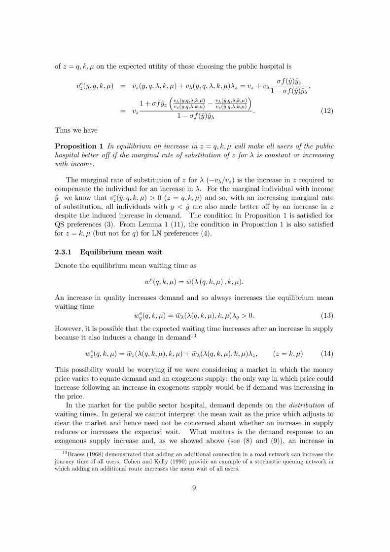
Thus we have

Proposition 1 In equilibrium an increase in z = q; k; ¹ will make all users of the publichospital better o¤ if the marginal rate of substitution of z for ¸ is constant or increasingwith income.

The marginal rate of substitution of z for ¸ (¡v¸=vz) is the increase in z required tocompensate the individual for an increase in ¸. For the marginal individual with incomey we know that vez(y; q; k; ¹) > 0 (z = q; k; ¹) and so, with an increasing marginal rateof substitution, all individuals with y < y are also made better o¤ by an increase in zdespite the induced increase in demand. The condition in Proposition 1 is satis…ed forQS preferences (3). From Lemma 1 (11), the condition in Proposition 1 is also satis…edfor z = k; ¹ (but not for q) for LN preferences (4).

2.3.1 Equilibrium mean wait

Denote the equilibrium mean waiting time as

we(q; k; ¹) = ¹w(¸ (q; k; ¹) ; k; ¹):

An increase in quality increases demand and so always increases the equilibrium meanwaiting time

weq(q; k; ¹) = ¹w¸(¸(q; k; ¹); k; ¹)¸q > 0: (13)

However, it is possible that the expected waiting time increases after an increase in supplybecause it also induces a change in demand13

wez(q; k; ¹) = ¹wz(¸(q; k; ¹); k; ¹) + ¹w¸(¸(q; k; ¹); k; ¹)¸z; (z = k; ¹) (14)

This possibility would be worrying if we were considering a market in which the moneyprice varies to equate demand and an exogenous supply: the only way in which price couldincrease following an increase in exogenous supply would be if demand was increasing inthe price.

In the market for the public sector hospital, demand depends on the distribution ofwaiting times. In general we cannot interpret the mean wait as the price which adjusts toclear the market and hence need not be concerned about whether an increase in supplyreduces or increases the expected wait. What matters is the demand response to anexogenous supply increase and, as we showed above (see (8) and (9)), an increase in

13Braess (1968) demonstrated that adding an additional connection in a road network can increase thejourney time of all users. Cohen and Kelly (1990) provide an example of a stochastic queuing network inwhich adding an additional route increases the mean wait of all users.

9

supply induces a change in the distribution of waiting times which increases the expectedutility for the marginal patient choosing public hospital and so increases demand.

To ensure that wez(q; k; ¹) < 0 (z = k; ¹) requires further restrictions on preferences or

on the distribution of waiting times generated by the queueing system.

Proposition 2 The equilibrium expected waiting time is decreasing in z = ¹; k if (a)preferences are linear in waiting time (4) or (b) equal increases in the arrival rate ¸ andin supply z leave the mean waiting time unchanged ( ¹wz = ¡ ¹w¸).

The proofs are in the Appendix. One example of a queueing process satisfying thesecond condition is M=M=1.14 We stress that none of the subsequent analysis requires theassumption that an increase in supply reduces the equilibrium mean waiting time, thoughit is sometimes useful in interpreting some of the results on optimal pricing rules.

2.3.2 Equilibria in deterministic and stochastic models.

Almost all waiting time models in the health economics literature assume that both de-mand and supply and hence the waiting time are certain. The purpose of this section isto highlight some qualitative di¤erences with our approach by comparing simple versionsof the stochastic and deterministic waiting time models.

Suppose that the stochastic queueing system is M=M=1 with a single server and anexponential distribution of waiting times and that patients have linear preferences (4) andso are concerned only with the expected waiting time ¹w which in the M=M=1 system isjust ¹w = 1=(¹ ¡ ¸). Hence demand is ¸(q; ¹w), with ¸q > 0, ¸ ¹w < 0. In Figure 1 , withthe service rate set at ¹0 the expected waiting time ¹w = 1=(¹0 ¡¸) increases with ¸ from(1=¹0) at ¸ = 0 and tends to in…nity as ¸ ! ¹. Because demand depends on the meanwaiting time, the equilibrium is determined by the intersection of the downward slopingdemand curve ¸(q0; ¹w) and the upward sloping expected waiting time locus ¹w = 1=(¹0¡¸).The equilibrium mean wait ¹w0 and the equilibrium expected number of patients treatedper period is ¸0 = ¸(q0; ¹w0).15 Note that the expected output (number of patients treatedper period) is equal to expected demand ¸(q0; ¹w0) and strictly less than the service rate¹0 which is the maximum possible expected output.

Suppose that a reduction in quality from q0 to q1 induces a parallel downward shift inthe demand curve to ¸(q1; ¹w). The new equilibrium is ¹w1 with lower mean waiting timeand a smaller expected number of patients ¸1 = ¸(q1; ¹w1) treated.

Now consider a deterministic waiting time process. Since both demand and servicetimes are certain so is the waiting time. In each period nature randomly picks a proportion¾ of patients to become ill, so that the number falling ill each period is certain but eachpatient faces the probability ¾ of falling ill. Expected utility for a patient who will choosethe public hospital when ill is

vD(y; q; wD) = ¾u(y; q;wD) + (1¡ ¾)uN(y);

14 In a "one bed"-hospital, w = 1¹¡¸ so that w¹ = ¡w¸.

15 In the usual stochastic queueing model demand is exogenous–there is no balking by patients, and theequilibrium mean wait is determined by the intersection of the ¹w = 1=(¹0 ¡ ¸) locus and the vertical lineat the exogenous arrival rate.

10

where wD is the certain wait in the deterministic system. To ensure that the demand curveis the same as in the stochastic case shown in Figure 1 we assume that patient preferencesare also given by (4). The certain demand for treatment in the public sector is

¸D(q;wD) = ¾F (yD(q;wD));

where the threshold income yD(q;w) is de…ned by

vD(y; q;wD)¡ V o(y ¡ °) = 0:

Hence in Figure 1 LN preferences ensure that the deterministic and stochastic demandcurves are identical: ¸D = ¸(q;wD) = ¸ (q; ¹w).

Figure 1. Equilibria in stochastic and deterministic waiting time models. wexpected waiting time in stochastic model, wD certain waiting time in deterministicmodel, ¸(q;w), expected demand in stochastic model, ¸(q; wD) certain demand in

deterministic model.

We denote the certain supply of treatments per unit of time as sD. This is a functionof hospital decisions a¤ecting length of stay, number of beds and so on. To comparethe stochastic and deterministic models we assume that the certain supply is equal to thenumber of beds times the service rate: sD = k¹, which in the special M=M=1 case inFigure 1 is just sD = ¹0.

With vwD < 0 the waiting time adjusts to clear the market: if ¸D exceeds sD thenumber waiting to be treated will increase and so will the waiting time, reducing thein‡ow of new patients until ¸(q; wD) = sD. Conversely if ¸D is less than sD the waitingtime will fall until either ¸(q;wD) = sD or ¸(q; 0) · sD. Since supply has a positivemarginal cost the hospital will never choose to have sD > ¸(q; 0).

In Figure 1 the initial equilibrium waiting time wD0 in the deterministic case is givenby the intersection of ¸(q0; wD) and the vertical supply curve at sD = ¹0. The certainequilibrium waiting time is less than the mean wait in the stochastic equilibrium becausewith certain demand and supply there will never be unused capacity: e¤ective supply islarger in the deterministic case and equal to the certain demand.

11

Increases in supply have the same qualitative e¤ects in the deterministic model and thestochastic models: equilibrium waiting time falls and the (expected) number of patientstreated increases.16 But the implications of a demand shift are di¤erent. A reduction inquality from q0 to q1 with unchanged supply will reduce the equilibrium certain waitingtime to wD1and the equilibrium expected waiting time to ¹w1. In the stochastic case theequilibrium expected output (patients treated) will also decrease to ¸1 = ¸(q1; ¹w1). Butin the deterministic case there is no reduction in equilibrium output which, by assumptionis equal to the unchanged supply. The deterministic equilibrium is re-established solelyby a reduction in waiting time so that demand is equated to unchanged supply. Thus inthe deterministic case a hospital whose revenue varies only with the number of patientstreated could increase its pro…t by reducing quality, shifting the certain demand curvedownwards, and allowing the certain waiting time to fall to keep demand and outputunchanged. In the stochastic waiting time speci…cation the hospital would lose revenueif it reduced quality. We examine the implications of this crucial di¤erence betweenstochastic and deterministic waiting time models for deriving optimal hospital paymentrules in Section 5.

2.4 Welfare function

2.4.1 Patient welfare

The patient welfare function is additive over individuals, with the bene…t to an individualbeing be(y; q; k; ¹) = b(y; q; ¸(q; k; ¹); k; ¹), (y 2 [ymin; ymax]) and total patient welfare

Be(q; k; ¹) =

Z ye(q;k;¹)

ymin

be(y; q; s)dF (y) +

Z ymax

ye(q;k;¹)bo(y; qo)dF (y);

with, for z = q; k; ¹,

Bez(q; k; ¹) =

Z ye(q;k;¹)

ymin

bez(y; q; k; ¹)dF (y) + [be(y; q; k; ¹)¡ bo(y ¡ °; qo)] f (ye) yez: (15)

We allow for the fact that the individual bene…t b(y; ¢) which the regulator takes intoaccount, may not coincide with the expected utility ve(y; ¢) on which citizens with incomey base their decision. Hence, the welfare of the marginal patient may not be the samein the public and private hospital.17 The speci…cation also re‡ects the assumption thatit is not possible to directly a¤ect the decision to seek public treatment except via q; kor ¹, so that y is determined by patient decisions, not by the regulator. In addition,we assume that the level of q; k and ¹ in the public sector does not a¤ect the insurancepremium, quality, or the waiting time in the private sector. With a utilitarian welfarefunction respecting patient preferences be(y; q; k; ¹) = ve(y; q; k; ¹), bo = vo(y¡°) and the

16Although by less than the capacity increase in the stochastic model since ¸¹ < 1 (cf (8)).17 For example, the regulator may be of the opinion that the individual bene…t should not vary with in-

come (b(q; k; ¸; ¹)), or that the marginal bene…t of attributes should be income independent (bz(q; ¸; k; ¹)),or that the marginal willingness to pay should be independent of income: bz(y;q;k;¸;¹)

by(y;q;k;¸;¹)= bz(q;k;¸;¹)

by(q;k;¸;¹). This

last is similar to what Tobin (1970: 264) called speci…c egalitarianism (“the view that certain speci…cscarce commodities should be distributed less unequally than the ability to pay for them.”)

12

last term in (15) vanishes because the marginal patient is indi¤erent between the sectors(see (5)).

In one speci…cation of the welfare function, with implications which we discuss inSection 3, patients have quasi separable preferences (3) which are partly respected by thewelfare function. The welfare of a patient choosing the public sector is

be(y; q; k; ¹) = ¾[m0(y) +m1(y)m2(Re(q; k; ¹))] + (1¡ ¾)mN(y); m2R > 0: (16)

In this case the welfare function respects patient preferencesRe(q; k; ¹) =R(¸(q; k; ¹); q; k; ¹)over characteristics of hospital treatment in the sense that the regulator’s marginal rate ofsubstitution of q for k or ¹ is the same as that of the patient. But the monetary valuationof hospital treatment characteristics, and so the willingness to pay, may di¤er.

2.4.2 Costs

The second component of the welfare function is the public hospital’s expected cost

cHe(q; k; ¹) = cH(q; ¸(q; k; ¹); k; ¹):

We assume that increasing quality is costly (cHq > 0) as are supply decisions (cHz > 0; z =k; ¹) which induce a more favourable distribution of waiting times. We also allow for thepossibility that expected hospital cost depend on the expected number of patients treated(¸), for example because each patient treated requires drugs and other consumables.18

The marginal cost of expected output is cH¸ > 0 and so cHez (q; k; ¹) = cHz + cH¸ ¸z > 0, (z =

q; k; ¹). We ignore, until section 4, the possibility that the cost of producing treatmentsof given quality can be a¤ected by cost reducing e¤ort.

We assume that patients do not work whilst waiting and are fully compensated forlost earnings with the cost of lost output borne by a social insurance fund. We normaliselabour supply when healthy to 1. Since the mean wait is we (q; k; ¹), the expected totalcompensation payment from the insurance fund (cIe) in equilibrium is

cIe(q; k; ¹) = ¾we (q; k; ¹)

Z ye(q;k;¹)

ymin

ydF (y):

An increase in attribute z(= q; k; ¹) alters expected insurance cost both by changing theexpected waiting time (waiting time e¤ect) and by changing the number of individualswaiting (waiting list e¤ect):

cIez = ¾wez

Z ye(q;s)

ymin

ydF (y) + ¾we (q; s) yef(ye)yez : (17)

Since yez > 0 (z = q; k; ¹), increases in quality and supply conditions induce richer patientsto join the waiting list and so increase the income loss at a given mean wait. An increase inquality also increases the waiting time (we

q = ¹w¸(¸; k; ¹)¸q > 0) and hence always increase

18We assume that in the steady state equilibrium the expected output rate equals the expected arrivalrate ¸. In queueing theory, this is property is known as Burke’s Theorem (Burke, 1956) and holds for theM=M=k system.

13

the compensation payment: cIeq > 0. As we noted in section 2.3.1 in general the e¤ect ofan increase in supply on the mean waiting time is ambiguous because whilst the increasein supply reduces the mean wait it also induces a partially o¤setting increase in demandwhich increases the mean wait: we

z = ¹wz + ¹w¸¸z (z = k; ¹). If we make the intuitiveassumption that we

z < 0 the sign of cIez is ambiguous.The regulator’s objective function is19 ;20

Ae(q; k; ¹)def= Be(q; k; ¹)¡ (1 + µ)Ce(q; k; ¹);

where µ is the marginal cost of public funds and

Ce(q; k; ¹)def= C(q; ¸(q; k; ¹); k; ¹) = cHe(q; k; ¹) + cIe(q; k; ¹): (18)

In the next sections, we inquire about the optimal hospital payment schemes underdi¤erent assumptions about which hospital decisions and outcomes can be observed.

3 Optimal payment schemes

We …rst derive …rst best levels of hospital quality and supply and then examine how theycan be implemented with payment schemes.21

3.1 First best regulation

Social welfare depends on hospital decisions about treatment quality (q), treatment inten-sity (¹) and the number of beds (k). The …rst best levels of these attributes satisfy the…rst order conditions

Aes = Be

s ¡ (1 + µ)Ces = Bq ¡ (1 + µ)Cs + [B¸ ¡ (1 + µ)C¸]¸s = 0; (s = ¹; k), (19)

Aeq = Be

q ¡ (1 + µ)Ceq = Bq ¡ (1 + µ)Cq + [B¸ ¡ (1 + µ)C¸]¸q · 0; q ¸ 0: (20)

The condition on q holds with complementary slackness: we allow for the possibility thatthe …rst best quality is minimal (q = 0) but ignore the trivial solution where no patients

19One set of assumptions which yields this form is that the regulator is only concerned with patientwelfare and tax …nanced public expenditure, and sets a lump sum tax or subsidy so that provider justbreaks even …nancially after any incentive payments. Or welfare is the sum of patient bene…t and thehospital utility and the lump sum tax or subsidy drives hospital utility to zero.

20 Implicitly, we renormalise patient bene…t to make it commensurable with the currency that costs aremeasured in. Since both patient utility (v) or the regulator’s perception of that utility (b) are cardinalfunctions, these can be rescaled by a positive constant.

Note that we could reformulate our model in terms of the willingness to pay for public treatment, P (y; ¢),de…ned as v(y ¡ P (y; ¢); ¢) = v0(y ¡ °) and measure social surplus as

R ye(q;¢)ymin P e(y; ¢)dF (y). The critical

citizen would have a willingness to pay P (by; ¢) = 0. Paternalistic social preferences would replace P e(y; ¢)by some other WTP function, also measured in the same currency as income and costs.

21Strictly, we are considering the second best because we are not giving the regulator the means todirectly control patient demand. Such control would correct for the externality that arises because themarginal patient ignores the e¤ect of her decision to join the waiting list on the average waiting time. SeeNoar (1969), Littlechild (1974), and Edelson and Hildebrand (1975) on policies to control decisions to jointhe queue.

14

are treated in the public sector (¹ = 0 and k = 0).To examine the circumstances in which …rst best quality is positive we use (19) to

substitute [Bs ¡ (1 + µ)Cs]=¸s for [B¸ ¡ (1 + µ)C¸] in (20) to get

Aeq =

µBq ¡Bs

¸q¸s

¶¡ (1 + µ)

µCq ¡Cs

¸q¸s

¶(s = ¹; k). (21)

The rate at which s must be reduced to keep demand constant after an increase in q is(¡¸q=¸s) so that …rst best quality is positive if, starting from q = 0, the net increase inpatient welfare from such a reform exceeds the net increase in production and insurancecost.22

From Theorem A.3 in the appendix

Beq ¡Be

s

¸q¸s

= Bq ¡Bs¸s¸q

=

Z y

ymin

bs(y; ¢)·bq(y; ¢)bs(y; ¢)

¡ vq(y; ¢)vs(y; ¢)

¸dF (y): (22)

We can sign the …rst term in (21) under some assumptions about welfare and patientpreferences. If the welfare function respects patient preferences in the sense that theregulator’s marginal rates of substitution between quality and supply variables are equalto those of patients then (22) is positive if the average marginal welfare valuation of qin terms of s is greater than the marginal valuation revealed by the demand responses ofthe marginal patient who is indi¤erent between the public and private hospital. If patientpreferences are quasi-separable and are respected in the welfare function then (22) is zero:the reform does not increase patient bene…t.

Next consider the net cost implications of increasing q and adjusting s (s = ¹; k) tokeep demand constant. From (18) and Lemma A5 (A.8), we have

Cq ¡Cs¸q¸s

=

µcHq ¡ cHs

¸q¸s

¶+

µcIq ¡ cIs

¸q¸s

¶;

=

µcHq ¡ cHs

¸q¸s

¶¡ ¾ ¹ws

Z y

ymin

ydF¸q¸s

(s = ¹; k).

If the marginal hospital cost of quality at zero quality is small then the overall e¤ect of thereform is to reduce hospital cost. Since the reform keeps demand constant the number ofpeople who require income compensation is unchanged and the e¤ect of the reform is toincrease expected insurance cost because the reduction in attribute s increases the averagewait. Thus while the overall e¤ect of the reform on cost is ambiguous, we may expect itto be negative if minimal quality in the public hospital encourages most citizens to takeout private insurance. So we conclude that …rst best quality is more likely to be aboveits minimal level when (i) patients with lower incomes have a higher marginal valuationof quality in terms of s, (ii) the marginal hospital cost of quality is low when quality isminimal, and (iii) the e¤ect of increases in the equilibrium wait on the total income lostdue to waiting is small at minimal quality.

22Equivalently, multiplying (19) through by ¸q¸s

and subtracting from (20) yields (21). By construction,

this reform gets rid of the indirect e¤ects on B and C due to changes in demand so that Beq ¡Be

s¸q¸s

= Bq

¡Bs¸q¸s

and Ceq ¡ Ce

s¸q¸s

= Cq ¡Cs¸q¸s

:

15

In what follows, we will assume that …rst best quality always exceeds the minimal level.

3.2 First best payment schemes

In general, we require as many policy instruments with linearly independent e¤ects onhospital decisions as the hospital has decision variables. The hospital makes decisionson q, ¹ and k which result in an expected number of treatments, ¸(q; ¹; k), as well as anexpected waiting time we(q; ¹; k). We will assume that it is always possible to observeoutput ¸ and so to set a prospective price per completed treatment p¸. It may alsobe possible to attach a price to quality pq (a pay for performance scheme), a (possiblynegative) price to the average wait (p ¹w), and to reward supply decisions via p¹ and to havea beds subsidy pk.23 With …ve instruments available to in‡uence three provider decisionsthere are 10 possible …rst best schemes. Given the increased use of prospective outputpricing, we examine three of the six pricing schemes which include a prospective outputprice p¸. In Section 4 we consider some examples of second best pricing schemes in whichthere is only one other instrument available in addition to the prospective price. We thendiscuss the third best prospective price when there are no other instruments. Finally,we allow for the possibility that unobserved provider e¤ort a¤ects cost and consider costreimbursement rules.

3.2.1 Payment for output, beds and average length of stay

We …rst assume that the risk neutral public hospital receives a payment per patient treated,p¸, per bed installed, pk, and per unit of service rate, p¹ – recall that average length ofstay is 1

¹ . The risk neutral public hospital chooses q, k and ¹ to maximise a weightedsum of expected pro…t and patient welfare with ® ¸ 0 re‡ecting the hospital’s degree ofconcern for patients. It also receives a lump sum transfer T (possibly negative) to ensurethat it breaks even:24

maxq;k;¹

p¸¸(q; k; ¹) + pkk + p¹¹¡ cHe(q; k; ¹) + ®Be(q; k; ¹) + T (23)

First order conditions for an interior solution are

p¸¸z + pk1(z=k) + p¹1(z=¹) + ®Bez = cHe

z (z = q; k; ¹) (24)

where 1(¢) is the indicator function equal to 1 if the condition (¢) is true and equal to zerootherwise. In the appendix (section A.5) we use a general approach to derive …rst, secondand third best prices. Here, we will focus on the main results and their interpretation.To shorten notation, we will de…ne the residual marginal social bene…t (RMSB) of decision

z as Sez

def= ¯Be

z ¡ cIez , where ¯def= 1¡®(1+µ)

1+µ . Sz denotes that part of the social welfaree¤ect of decision z which is not internalised by the hospital. Recall that the hospital

23 In addition to the prospective output price Chalkley and Malcomson (1998) also consider linkingpayment to the number of patients not treated but added to a waiting list. However, the costs of deferredtreatment for these patients is implicitly assumed to be zero and so both the …rst best and the paymentmechanism required to achieve it take no account of the costs of rationing demand.

24Hospital pro…t is ¼ = p¸¸(q; k; ¹)+pkk+p¹¹¡ cHe(q; k; ¹)+T . For ¼ to be zero, T = ¡p¸¸¡pkk¡p¹¹+ c(q; k; ¹). The hospital perceives T as lump sum.

16

takes into account a fraction ® of patient bene…t, as well as the entire hospital cost (see(23)). Hence, Se

z , is the remaining part, ’discounted’ by the marginal cost of publicfunds. The conditions for …rst best imply that Se

z > 0 (z = q; k; ¹). First best prices onquality, beds and service rate would be set at Se

z (z = q; k; ¹), the superscript e indicatingthat demand responses are taken into account–a result of the fact that demand is notdirectly controlled by the planner: thus Se

z = Sz + S¸¸z (z = q; k; ¹). However, we areassuming that quality is not observed and that instead a price is attached to output, ¸,which is a good substitute because demand (and therefore output) is sensitive to qualityof treatment. In the Appendix, we show

Proposition 3 The …rst best prices per treated patient, bed and unit of service rate are

pFB¤¸ =

Seq

¸q; (25)

pFB¤k = Se

k ¡ pFB¤¸ ¸k (26)

pFB¤¹ = Se

¹ ¡ pFB¤¸ ¸¹ (27)

where all terms on the right hand sides are evaluated at the …rst best quality, service rateand number of beds.

The …rst expression re‡ects the fact that rewarding output incentivises quality choice.

SinceSeq¸q

= ¯Beq

¸q¡ cIeq

¸q, the …rst best output price pFB¤

¸ is less than the marginal social

bene…t per patient attracted by higher quality³Beq

¸q

´to the extent that (i) hospitals are

intrinsically motivated, (ii) raising public funds is costly, and (iii) a quality increase resultsin larger social insurance expenditure because it attracts more to public treatment if illand therefore increases the waiting time and the waiting list. To bring this out starkly,suppose that the provider is not altruistic (® = 0) and that there is no loss of earningswhilst waiting for treatment. Then (25) can be written as pFB

¸ ¸q = Beq= (1 + µ), so that

the provider’s marginal revenue from increasing quality should be less than the marginalpatient welfare from higher quality only because of the marginal deadweight cost of publicfunds.

The remaining prices are adjusted for the fact that choice of beds and service rateare also rewarded through output, and should therefore be rewarded at a lower rate thantheir RMSB would require. Substituting for pFB¤

¸ , the prices for z (z = k; ¹) are pFB¤z =

Sez ¡ Se

q¸z¸q

and making use of (A.3) and (A.7), they can be written as

pFB¤z = ¯

Z ye(q;k;¹)

ymin

bq(y; ¢)·bz(y; ¢)bq(y; ¢)

¡ vz(by; ¢)vq(by; ¢)

¸dF (y)

¡¾wz(q; k; ¹)

Z ye(q;k;¹)

ymin

ydF (y) (z = k; ¹): (28)

The …rst term is the e¤ect of an increase in hospital decision z (z = k; ¹) on expectedpatient bene…t when quality is simultaneously reduced in order to keep demand, ¸, con-stant. bz

bqis the regulator’s perception of citizen y’s marginal valuation for quality in terms

of hospital attribute z, while bvzbvq is the corresponding valuation for individual y. If the

17

regulator respects individual preferences, bz(y;¢)bq(y;¢) =

vz(y;¢)vq(y;¢) and the …rst term will be positive

(negative) if the marginal valuation for quality in terms of income increases uniformlyfaster (slower) with income than that for attribute z (cf (A.6)). If both increase equallyfast, which is the case of quasi-separable preferences, the …rst term vanishes. The …rstterm also vanishes when the regulator’s perception of the preferences of the person withincome y respects their quasi-separable structure. The second term is the reduction insickness leave compensation because of a reduction in average wait. Both e¤ects call fora positive incentive for supply decision z (z = k; ¹).

3.2.2 Payment for patients, beds, and quality

Next suppose that the prospective output price is combined with prices linked to qualityand the number of beds. The rationale given for the pricing structure stated in Proposition3 immediately suggests

Proposition 4 The …rst best prices for output, beds, and quality are

pFB¤¤¸ =

Se¹

¸¹

pFB¤¤k = Se

k ¡ pFB¤¤¸ ¸k

pFB¤¤q = Se

q ¡ pFB¤¤¸ ¸q

where all terms on the right hand sides are evaluated at the …rst best quality, service rateand number of beds.

Since ¹ is not priced, rewarding treated patients becomes a substitute for rewardingthe service rate. The rewards per bed and quality unit re‡ect the MRSB, marked-downto take into account that these attributes are indirectly rewarded through the prospectiveoutput price.

3.2.3 Payment for output, beds and waiting times

Now consider combining a prospective price for output with a beds subsidy and a pricelinked to the mean waiting time. In the hospital’s objective function (23) pwwe(q; k; ¹) issubstituted for p¹¹, while the generic …rst order condition for attribute z turns into

p¸¸z + pwwez + pk1(z=k) + ®Be

z = cHez (z = q; k; ¹):

In the appendix, we prove

Proposition 5 The …rst best prices for mean wait, treated patients, and beds are

pFB+w =

µ¡ dS

d¹

¯¯d¸=0;dk=0

¶

(¡w¹); (29)

pFB+¸ =

Seq

¸q¡ pFB+

w w¸; (30)

pFB+k = Se

k ¡ pFB+¸ ¸k ¡ pFB+

w wk: (31)

18

The substitution of w for ¹ in the reward scheme (27) intuitively replaces pFB¤¹ =µ

¡ dSd¹

¯¯d¸=0;dk=0

¶with (29). Since a reward for the waiting time now indirectly rewards

output as well to the extent that the average wait is responsive to demand (w¸ > 0), thisleads to a smaller …rst best reward per patient treated as given by (30). The reward perbed is adjusted accordingly (31).25

Since w¹ < 0, it transpires from (29) that pFB+w should take the opposite sign of pFB¤

¹ ,

given by (28). Thus if b¹(y;¢)bq(y;¢) is su¢ciently smaller than bv¹

bvq (e.g., when b¹(y;¢)bq(y;¢) =

v¹(y;¢)vq(y;¢) and

the marginal valuation for the service rate in terms of income rises su¢ciently faster withincome than that for quality) low income people are regarded to be better o¤ with higherquality and length of stay. It is then optimal to have a negative price on the service rateand therefore a positive price on the average wait. The waiting time is then a signal ofquality and length of stay, and subsidising it will promote both attributes.

4 Second and third best prospective output pricing

4.1 Second best output and mean wait prices

We now assume that the regulator can observe only the output and the mean waitingtime. The hospital’s objective function is now p¸¸(q; k; ¹) +pww

e(q; k; ¹) +®Be(q; k; ¹)¡cHe(q; k; ¹) and its choices satisfy the …rst order conditions

p¸¸z + pwwez + ®Be

z = cHez (z = q; k; ¹): (32)

Before inquiring about the optimal second best price levels for p¸ and pw, notice thatthe hospital is left with some discretion in the second best since it makes decisions onthree attributes, q; k and ¹, while incentives are provided on two outcomes, ¸ and w. Inresponse to a marginal change in the output price, the three attribute levels are adjusted,@z@p¸

(z = q; k; ¹), resulting in an increase in the expected number of patients treated,@¸¤@p¸

def=P

z ¸z@z@p¸

and a change in the expected wait @w¤@p¸

def=P

z wez@z@p¸

.26 Likewise, a

marginal change in pw triggers responses @z@pw

(z = q; k; ¹) that result in an increase in the

25 It can be shown that0@

pFB+¸

pFB+k

pFB+w

1A =

0B@

1 0 ¡w¸w¹

0 1 ¡wkw¹

0 0 1w¹

1CA

0@

pFB¤¸

pFB¤

k

pFB¤¹

1A ;

indicating the recursive relationship between (25)-(27) and (29)-(31). The ratios ¡wzw¹

(z = ¸; k) adjustthe …rst best rewards for output and bed in a way that keeps the waiting time constant, and the reason isthat w is now separately incentivised. A third way of writing the …rst best price for output is by usingthe equilibrium waiting time e¤ects we

z (z = ¹; q):

pFB+¸ =

(¡we¹¸q)

¸¹weq + (¡¸qwe

¹)

Seq

¸q+

weq¸¹

¸¹weq + (¡¸qwe

¹)

Se¹

¸¹;

i.e., a weighted average of the MRSB for quality and service rate, the two hospital attributes that are notdirectly rewarded by the present scheme.

26The equilibrium demand and expected waiting time are ¸¤(p¸; pw) = ¸(q(p¸; pw); k(p¸; pw); ¹(p¸; pw))and w¤(p¸; pw) = we(q(p¸; pw); k(p¸; pw); ¹(p¸; pw)).

19

expected wait, @w¤@pw

def=P

z wez

@z@pw

and a change in expected output @¸¤@pw

def=P

z ¸z@z@pw

.27

Consider now the induced response change in output following an increase in p¸ when w¤

is kept …xed. This hospital response is given by @¸¤@p¸

¡ @¸¤@pw

³@w¤@pw

´¡1@w¤@p¸

.28 Likewise,the optimal change in bed use following an increase in p¸ when w¤ is kept …xed, is given

by @k@p¸

¡ @k@pw

³@w¤@pw

´¡1@w¤@p¸

. As a result, when w¤ is kept constant, the induced responsee¤ect on outcome ¸ per unit change in decision k can be de…ned as

¸irk jdw=0

def=

@¸¤@p¸

¡ @¸¤@pw

³@w¤@pw

´¡1@w¤@p¸

@k@p¸

¡ @k@pw

³@w¤@pw

´¡1@w¤@p¸

: (33)

In the same vein, we can de…ne the induced response e¤ect on outcome we per unitchange in k when keeping ¸ …xed :

wirk jd¸=0

def=

@w¤@pw

¡ @w¤@p¸

³@¸¤@p¸

´¡1@¸¤@pw

@k@pw

¡ @k@p¸

³@¸¤@p¸

´¡1@¸¤@pw

: (34)

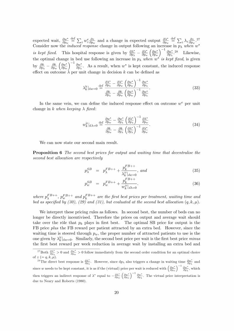
We can now state our second main result.

Proposition 6 The second best prices for output and waiting time that decentralise thesecond best allocation are respectively

pSB¸ = pFB++¸ +

pFB++k

¸irk jdw=0

, and (35)

pSBw = pFB++w +

pFB++k

wirk jd¸=0

: (36)

where pFB++¸ , pFB++

w and pFB++k are the …rst best prices per treatment, waiting time and

bed as speci…ed by (30), (29) and (31), but evaluated at the second best allocation (q; k; ¹).

We interpret these pricing rules as follows. In second best, the number of beds can nolonger be directly incentivised. Therefore the prices on output and average wait shouldtake over the rôle that pk plays in …rst best. The optimal SB price for output is theFB price plus the FB reward per patient attracted by an extra bed. However, since thewaiting time is steered through pw, the proper number of attracted patients to use is theone given by ¸ir

k jdw=0. Similarly, the second best price per wait is the …rst best price minusthe …rst best reward per week reduction in average wait by installing an extra bed and

27Both @¸¤@p¸

> 0 and @w¤@pw

> 0 follow immediately from the second order condition for an optimal choiceof z (= q; k; ¹).

28The direct best response is @¸¤@p¸

. However, since dp¸ also triggers a change in waiting time @w¤@p¸

and

since w needs to be kept constant, it is as if the (virtual) price per wait is reduced with³@w¤@pw

´¡1@w¤@p¸

, which

then triggers an indirect response of ¸¤ equal to ¡ @¸¤@pw

³@w¤@pw

´¡1@w¤@p¸

. The virtual price interpretation is

due to Neary and Roberts (1980).

20

keeping output constant (assuming wirk jd¸=0 < 0). Thus the fact that w (¸) is still priced

calls for the use of induced responses in the pricing rule for ¸ (w) that are conditioned onthe outcome w (¸).

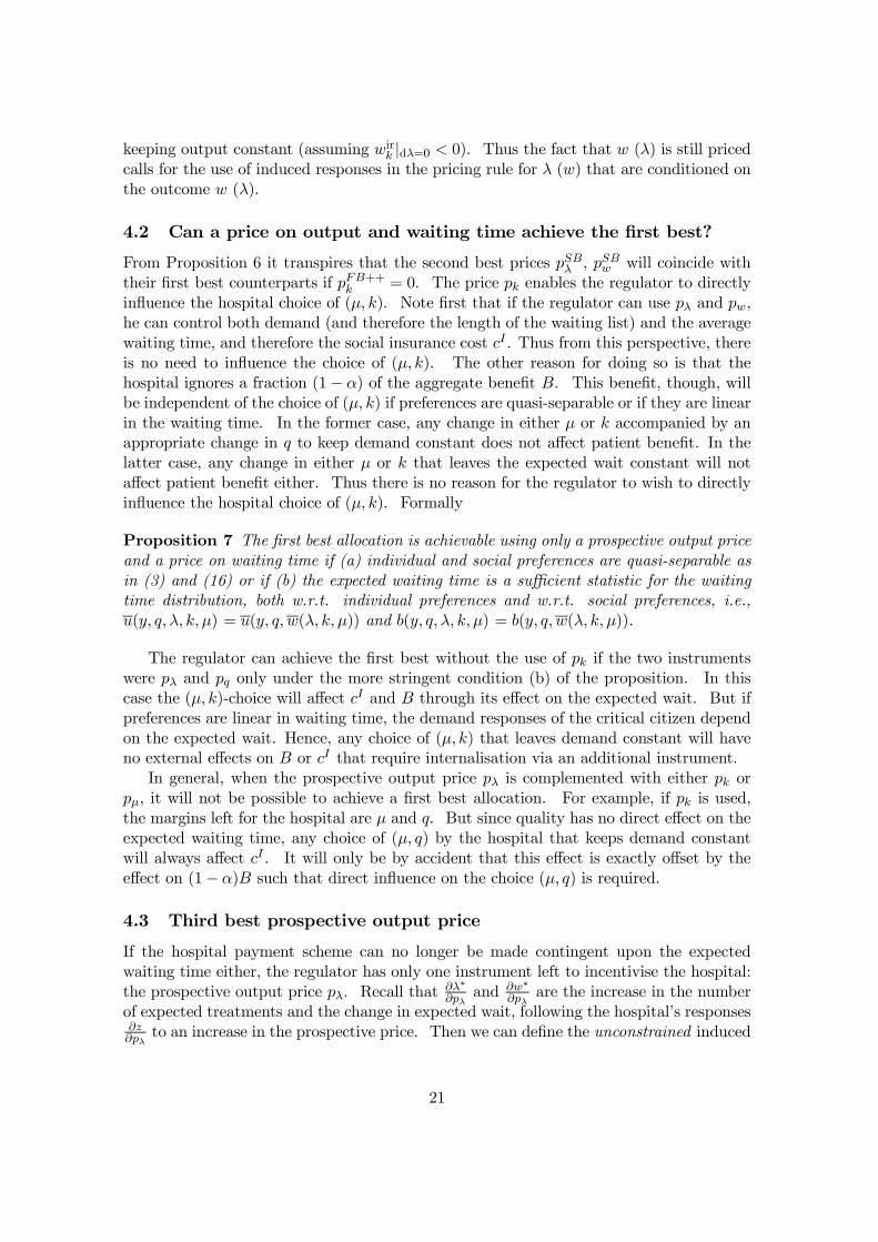
4.2 Can a price on output and waiting time achieve the …rst best?

From Proposition 6 it transpires that the second best prices pSB¸ , pSBw will coincide withtheir …rst best counterparts if pFB++

k = 0. The price pk enables the regulator to directlyin‡uence the hospital choice of (¹; k). Note …rst that if the regulator can use p¸ and pw,he can control both demand (and therefore the length of the waiting list) and the averagewaiting time, and therefore the social insurance cost cI . Thus from this perspective, thereis no need to in‡uence the choice of (¹; k). The other reason for doing so is that thehospital ignores a fraction (1¡ ®) of the aggregate bene…t B. This bene…t, though, willbe independent of the choice of (¹; k) if preferences are quasi-separable or if they are linearin the waiting time. In the former case, any change in either ¹ or k accompanied by anappropriate change in q to keep demand constant does not a¤ect patient bene…t. In thelatter case, any change in either ¹ or k that leaves the expected wait constant will nota¤ect patient bene…t either. Thus there is no reason for the regulator to wish to directlyin‡uence the hospital choice of (¹; k). Formally

Proposition 7 The …rst best allocation is achievable using only a prospective output priceand a price on waiting time if (a) individual and social preferences are quasi-separable asin (3) and (16) or if (b) the expected waiting time is a su¢cient statistic for the waitingtime distribution, both w.r.t. individual preferences and w.r.t. social preferences, i.e.,u(y; q; ¸; k; ¹) = u(y; q; w(¸; k; ¹)) and b(y; q; ¸; k; ¹) = b(y; q; w(¸; k; ¹)).

The regulator can achieve the …rst best without the use of pk if the two instrumentswere p¸ and pq only under the more stringent condition (b) of the proposition. In thiscase the (¹; k)-choice will a¤ect cI and B through its e¤ect on the expected wait. But ifpreferences are linear in waiting time, the demand responses of the critical citizen dependon the expected wait. Hence, any choice of (¹; k) that leaves demand constant will haveno external e¤ects on B or cI that require internalisation via an additional instrument.

In general, when the prospective output price p¸ is complemented with either pk orp¹, it will not be possible to achieve a …rst best allocation. For example, if pk is used,the margins left for the hospital are ¹ and q. But since quality has no direct e¤ect on theexpected waiting time, any choice of (¹; q) by the hospital that keeps demand constantwill always a¤ect cI . It will only be by accident that this e¤ect is exactly o¤set by thee¤ect on (1¡ ®)B such that direct in‡uence on the choice (¹; q) is required.

4.3 Third best prospective output price

If the hospital payment scheme can no longer be made contingent upon the expectedwaiting time either, the regulator has only one instrument left to incentivise the hospital:the prospective output price p¸. Recall that @¸¤

@p¸and @w¤

@p¸are the increase in the number

of expected treatments and the change in expected wait, following the hospital’s responses@z@p¸

to an increase in the prospective price. Then we can de…ne the unconstrained induced

21

responses in ¸ and w following the hospital responses to a marginal increase in p¸ as

¸irk

def=

@¸¤@p¸@k@p¸

and wir¸

def=

@w¤@p¸@¸¤@p¸

: (37)

Using these de…nitions we can characterise the third-best prospective output price:

Proposition 8 The price for output that decentralises the third best allocation is given by

pTB¸ = pFB+++¸ +wir

¸ £ pFB+++w +

pFB+++k

¸irk

: (38)

where pFB+++¸ , pFB+++

w and pFB+++k are the …rst best prices per treatment and bed as

speci…ed by (30), (29) and (31) but evaluated at the third best allocation of q; ¹ and k.

Suppose @w¤@p¸

> 0 and @k@p¸

> 0. Then wir¸ > 0 and ¸ir

k > 0 and the third best outputprice is the …rst best price with two mark-ups: one equal to the …rst best reward for anextra bed per patient attracted and another equal to the extra reward that the …rst bestprice on waiting time (possible negative) would have triggered per attracted patient. Thusthe third best price for output picks up the incentives on bed installment and service ratedecisions (the latter through incentivising the waiting time). Unlike in (33) and (34) theinduced responses de…ned in (37) are no longer conditioned on a …xed wait or demand.The reason is that the average wait is no longer separately incentivised. In this sense, thethird best output price is less sophisticated than the second best price.

The prospective output price by itself yields the …rst best only under stringent as-sumptions:

Proposition 9 The …rst best allocation is achievable using only a prospective output priceif individual and social preferences are quasi-separable and sickness leave compensation iszero.

With QS preferences, the only role for pw is to make the hospital aware of the con-sequences of its choice of (¹; k) for social insurance outlays. Without any sickness leavecompensation, e.g., because people can continue working while waiting for treatment, thisrole disappears. If people had LN preferences as in (4), additional instruments are requiredsince (¹; k) will in general a¤ect w and therefore patient bene…t.

4.4 Cost reducing e¤ort

So far we have ignored the possibility that the hospital can exert unobservable e¤ort toreduce production cost cH . If the hospital bears all the production cost it has the incentiveto select e¢cient cost reducing e¤ort. However, this presumes that the regulator hasa su¢cient set of instruments available in order to provide the hospital with the rightincentives at the other margins – quality, service rate and number of beds.

If the regulator has insu¢cient instruments to control quality, service rate and numberof beds, cost sharing will become optimal. For example, if the hospital is rewardedper treated patient and receives a price (possibly negative) per week of average wait,

22

but is not incentivised along the bed dimension, cost-sharing can be a useful second-bestinstrument because it indirectly subsidises the installation of extra beds. To make thisclaim more precise, suppose that the hospital is refunded a fraction ' of its productioncost cHe(q; ¹; k; t) where t is cost-reducing e¤ort which imposes non-veri…able cost g(t)on the hospital. Suppose also that it receives a lump sum to ensure that it breaks even…nancially29 and in the second best faces a prices on output and waiting time and in thethird best there is only a price on output. The cost sharing parameter and the pricesdetermine its decisions on q; ¹; k and t, which determine demand and the expected waitingtime we. De…ne the induced response marginal costs of an extra bed as

MCirk

¯d¸=0

def=

@cH¤@'

¯¯d¸=0

@k@'

¯¯d¸=0

; and

MCirk

¯d¸=0;dw=0

def=

@cH¤@'

¯¯d¸=0;dw=0

@k@'

¯¯d¸=0;dw=0

;

where @cH¤@' is the ensuing increase in hospital cost when the cost-share parameter increases

and the hospital adjusts its decisions on q; ¹; k and t to maximise its utility, @k@' is the

change in the number of beds and the vertical bars indicates that these induced responsesare conditioned on the output rate and, in the second best, the waiting time remainingconstant. Then we have (see Appendix):

Proposition 10 Suppose that (i) the hospital can reduce its cost by exerting an e¤ortwhich has an unveri…able cost, (ii) the regulator rewards per treated patient and possiblyalso per unit of waiting time, and (iii) the …rst-best reward per bed is pFB

k and per unit ofwaiting time is pFB

w . Then the second-best value for the cost-sharing parameter, 'SBcs,and the third-best value of that parameter when waiting time cannot be rewarded, 'TBcs,respectively satisfy

'SBcs £MC irk jdw=0

d¸=0 = pFB++k ; and (39)

'TBcs £MCirk jd¸=0 = pFB+++

k + pFB+++w £ bwir

k jd¸=0: (40)

where ++ (+++) indicates that the …rst-best prices are evaluated at the optimal second

(third) best values for the decision variables and bwirk jd¸=0

def=

@we¤@'

jd¸=0

@k@'

jd¸=0, the induced response

e¤ect of beds on the expected wait.

In second-best, when the waiting time is observable and rewardable, the responses usedto calculate the induced response marginal costs are conditional on ¸ and w being heldconstant (since both are directly rewarded). Expression (39) then shows that the optimalsecond-best refund of the marginal cost of installing an extra bed should coincide to the…rst-best bed reward; i.e., what is given as a direct subsidy in …rst-best should comes asa cost refund in second-best. When w can no longer be rewarded, we enter a third-best

29The break-even condition includes the non-veri…able cost of e¤ort.

23

situation. The proper induced marginal cost of an extra bed is then based on hospitalresponses that keep ¸ constant (because ¸ is still directly rewarded). According to (40),the third-best refund of the induced marginal cost of an extra bed amounts to the …rst-best bed reward plus the extra revenue the hospital would receive through the …rst-bestwaiting time reward. Thus cost sharing act as a good (but not perfect) substitute fordirect incentives at the cost of distorting the choice of cost-reducing e¤ort.

5 Optimal pricing with certain waiting time

We now contrast our results with those from a deterministic waiting time model. With thesame patient and regulator preferences over waiting time and quality as in the stochasticcase, patient welfare is

BD(q; wD) =

Z yD

ymin

b(y; q; wD)dF (y):

In addition to choosing quality, the hospital makes supply decisions which a¤ect the maxi-mum number of patients who can be treated each period (sD). We do not need to specifythese decisions in detail but to retain as many similarities with the stochastic speci…cationas possible we could assume that hospital capacity is give by the number of beds multipliedby the number of patients treated in each bed per period: sD = k¹. Whether made by theregulator or the hospital, these decisions minimise the cost of treating any given volumeof patients at a given quality. Hence we can write the hospital cost as cHD(¸D; q; sD) sothat, as in the stochastic case we allow for direct treatment costs to increase with thenumber treated (cHD

¸ > 0).The welfare function is then

AD = BD(q;wD)¡ (1 + µ)£cHD(¸D; q; sD) + cDI(q;wD)

¤; (41)

where

cDI = ¾wD

Z yD(q;wD)

ymin

ydF (y)

is the insurance cost of lost working time.The …rst best quality, waiting time, and supply are chosen to maximise (41) subject

to non-negativity constraints on quality and the waiting time and the market clearingcondition which determines the waiting time. Since supply is costly it will never bewelfare maximising to have ¸D > sD and so we can substitute ¸D(q;wD) for sD in thehospital cost function. The …rst order conditions for a welfare maximum are

BDq ¡ (1 + µ)

£cHD¸ ¸Dq + cHD

q + cHDs ¸Dq + cDI

q

¤· 0; q ¸ 0;

BDw ¡ (1 + µ)

£cHD¸ ¸Dw + cHD

s ¸Dw + cDIw

¤· 0; wD ¸ 0;

where the conditions on q and wD hold with complementary slackness.There are four possible …rst best con…gurations of quality and waiting time: (i) positive

quality and waiting time; (ii) quality and waiting time both zero; (iii) positive quality and

24

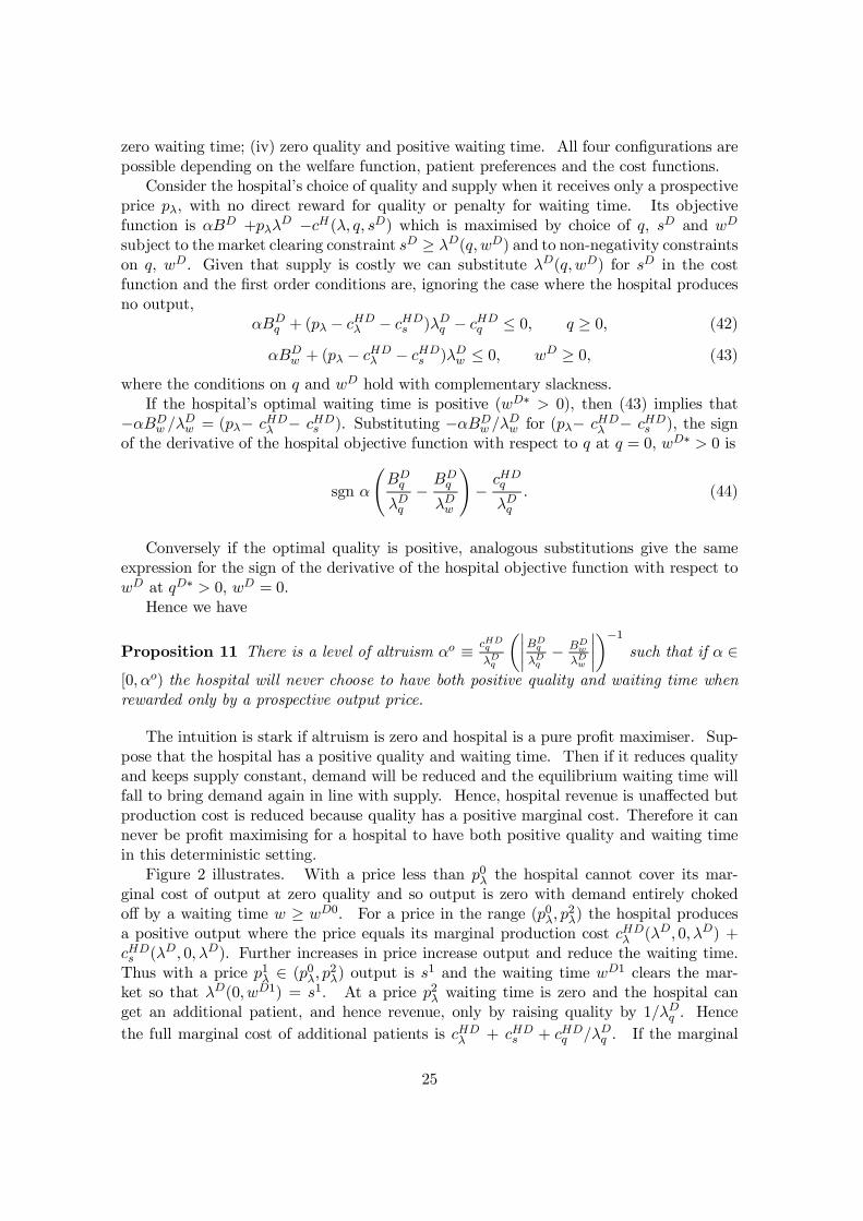
zero waiting time; (iv) zero quality and positive waiting time. All four con…gurations arepossible depending on the welfare function, patient preferences and the cost functions.

Consider the hospital’s choice of quality and supply when it receives only a prospectiveprice p¸, with no direct reward for quality or penalty for waiting time. Its objectivefunction is ®BD +p¸¸

D ¡cH(¸; q; sD) which is maximised by choice of q, sD and wD

subject to the market clearing constraint sD ¸ ¸D(q; wD) and to non-negativity constraintson q, wD. Given that supply is costly we can substitute ¸D(q;wD) for sD in the costfunction and the …rst order conditions are, ignoring the case where the hospital producesno output,

®BDq + (p¸ ¡ cHD

¸ ¡ cHDs )¸Dq ¡ cHD

q · 0; q ¸ 0; (42)

®BDw + (p¸ ¡ cHD

¸ ¡ cHDs )¸Dw · 0; wD ¸ 0; (43)

where the conditions on q and wD hold with complementary slackness.If the hospital’s optimal waiting time is positive (wD¤ > 0), then (43) implies that

¡®BDw =¸Dw = (p¸¡ cHD

¸ ¡ cHDs ). Substituting ¡®BD

w =¸Dw for (p¸¡ cHD¸ ¡ cHD

s ), the signof the derivative of the hospital objective function with respect to q at q = 0, wD¤ > 0 is

sgn ®

ÃBDq

¸Dq¡ BD

q

¸Dw

!¡ cHD

q

¸Dq: (44)

Conversely if the optimal quality is positive, analogous substitutions give the sameexpression for the sign of the derivative of the hospital objective function with respect towD at qD¤ > 0; wD = 0.

Hence we have

Proposition 11 There is a level of altruism ®o ´ cHDq

¸Dq

µ¯¯BD

q

¸Dq¡ BD

w

¸Dw

¯¯¶¡1

such that if ® 2[0; ®o) the hospital will never choose to have both positive quality and waiting time whenrewarded only by a prospective output price.

The intuition is stark if altruism is zero and hospital is a pure pro…t maximiser. Sup-pose that the hospital has a positive quality and waiting time. Then if it reduces qualityand keeps supply constant, demand will be reduced and the equilibrium waiting time willfall to bring demand again in line with supply. Hence, hospital revenue is una¤ected butproduction cost is reduced because quality has a positive marginal cost. Therefore it cannever be pro…t maximising for a hospital to have both positive quality and waiting timein this deterministic setting.

Figure 2 illustrates. With a price less than p0¸ the hospital cannot cover its mar-ginal cost of output at zero quality and so output is zero with demand entirely chokedo¤ by a waiting time w ¸ wD0. For a price in the range (p0¸; p

2¸) the hospital produces

a positive output where the price equals its marginal production cost cHD¸ (¸D; 0; ¸D) +

cHDs (¸D; 0; ¸D). Further increases in price increase output and reduce the waiting time.Thus with a price p1¸ 2 (p0¸; p

2¸) output is s1 and the waiting time wD1 clears the mar-

ket so that ¸D(0; wD1) = s1. At a price p2¸ waiting time is zero and the hospital canget an additional patient, and hence revenue, only by raising quality by 1=¸Dq . Hencethe full marginal cost of additional patients is cHD

¸ + cHDs + cHD

q =¸Dq . If the marginal

25

cost of quality at zero quality and output sD2 is positive there will be a range of prices[p2¸; p

3¸] over which output and quality do not vary with price. Once the price exceeds p3¸

= cHD¸ (s2; 0; s2) +cHD

s (s2; 0; s2) +cHDq (s2; 0; s2)=¸Dq (0; 0) the hospital will increase quality,

with zero waiting time, to attract additional patients as price increases. Thus at a pricep4¸, there will be s4 patients receiving immediate treatment.

Figure 2. E¤ect of prospective output price on quality, output, and waitingtime in deterministic waiting time model.

The implication of Proposition 11 is that with rationing by deterministic waiting timeit is impossible to achieve a …rst best allocation which has positive quality and waitingtime if the regulator is restricted to a prospective output price. If the demand for elec-tive hospital care is rationed by waiting time then it is necessary to be speci…c aboutthe rationing mechanism when modelling the behaviour of hospitals and examining thewelfare implications of incentive schemes. But the apparently convenient simpli…cation ofassuming that demand and supply, and hence waiting time, are certain is not satisfactoryin this context.

6 Conclusion

In this paper we have expanded previous analyses of optimal payment schemes for hospitalsby taking explicit account of the facts that demand and treatment time are random andthat patients care about waiting time. Queueing theory shows that under reasonableassumptions the stochastic processes generating demand and treatment time result inan equilibrium distribution of waiting times. However, unlike queueing theory whichusually takes the demand (arrival) process as exogenous, we examine rational expectationsequilibria in which patient decisions to join the waiting list depend on the equilibriumdistribution of waiting times and their decisions give rise to the equilibrium distribution.Even when the mean waiting time is a su¢cient statistic for patients when making their

26

provider choices, our stochastic model has properties that are qualitatively di¤erent fromthose that model the waiting time as a deterministic ‘price’ that balances demand andtreatment capacity.

We develop a general queueing model and use it to derive the optimal …rst best andsecond best pricing rules for a hospital providing care to fully insured patients. In generalthree prices are required ensure that the hospital chooses the welfare maximising quality,the service intensity determining average length of stay, and the number of beds. The …rstbest price per patient treated should be equal to the residual marginal social bene…t oftreating an extra patient. This is the part of the social bene…t which the hospital ignores:some or all of the direct bene…t of treatment plus the expected income loss to patientswhilst they are on the waiting list. In addition to the …rst best prospective output pricetwo other instruments are required. Candidates are a per bed subsidy, payments (possiblynegative) linked to the average waiting time and average length of stay, and payment forquality. In a second best, when the regulator can only link payment to the number ofpatients treated and to the expected waiting time, we show that the optimal price perpatient is the …rst-best price plus a mark-up that re‡ects the extra …nancing the hospitalwould have obtained in the …rst best by expanding the number of beds needed to attractan extra patient while at the same time keeping the expected wait constant (Proposition6, (35)). And vice versa, the optimal reward per waiting time (possibly negative) shouldbe set at the …rst best level minus the reward the hospital would have earned in …rst bestby expanding the number of beds to reducing the expected wait while keeping (expected)demand constant ((36)). In other words, second-best prices should pick up the unavailable…rst best incentives, but the way they is done depends on the set of prices available in thesecond best.

When the hospital can exert e¤ort to reduce its costs it is not necessary to directlyincentivise such e¤ort in the …rst best since it bears both production and e¤ort costs. Butin the second best it is optimal to refund a fraction of the total cost. This fraction shouldbe set such that the refund of the marginal cost of installing an extra bed re‡ects theoptimal …rst bed subsidy for such a bed (Proposition 10, (39)).

References

Aarbu, K. (2010). Demand patterns for treatment insurance in Norway. Ch 2 in Em-pirical essays on risk taking and insurance, PhD thesis, Norwegian School of Economics.

Besley, T., Hall, J., Preston I. (1999). The demand for private health insurance: Dowaiting lists matter? Journal of Public Economics 72, 155–181.

Braess, D. (1968). Über ein paradoxon aus der verkehrsplanung. Unternehmensforschung,12, 258–268. English translation: Braess, D., Nagurney, A., Wakolbinger, T. (2005). Ona paradox of tra¢c planning. Transportation Science, 39, 446-450.

Burke, P., (1956). The output of a queuing system. Operations Research 4, 699-704.Chalkley, M., Malcomson, J. (1998). Contracting for health services with unmonitored

quality. Economic Journal, 108 (449), 1093-1110.Chalkley, M., Malcomson, J. (2000). Government purchasing of health services. In

Culyer, A. Newhouse, J. (eds.), Handbook of Health Economics, Volume 1. North Holland,Amsterdam.

27

Cohen, J., Kelly, F. (1990). A paradox of congestion in a queuing network. Journal ofApplied Probability, 27, 730-734.

Cullis, J., Jones, P., Propper, C. (2000). Waiting lists and medical treatment: analysisand policies. In: Culyer, A.J., Newhouse, J.P. (Eds.), Handbook of Health Economics,North-Holland, Amsterdam

Edelson, N., Hildebrand, K. (1975). Congestion tolls for Poisson queueing processes.Econometrica, 43, 81-92.

Ellis, R., McGuire, T. (1986). Provider behavior under prospective reimbursement:cost sharing and supply, Journal of Health Economics, 5, 129-151.

Fomundam, S., Herrmann, J. (2007). A survey of queuing theory applications inhealthcare. ISR report 2007-24, University of Maryland.

Goddard, J., Malek, M., Tavakoli, M. (1995). An economic model for hospital tream-tent for non-urgent conditions, Health Economics 4, 41-55.

Gravelle, H., Dusheiko, M., Sutton, M. (2002).The demand for elective surgery in apublic system: time and money prices in the UK National Health Service, Journal ofHealth Economics, 21, 423-449

Gravelle, H., Siciliani, L. (2008). Optimal quality, waits and charges in health insur-ance. Journal of Health Economics, 27, 663-674.

Gross, D. Shortle, J., Thompson, J., Harris, C. (2008). Fundamentals of queueingtheory (3th ed.) (New York: Wiley).

Hassin, R., Haviv, M. (2003) To Queue or not to Queue: Equilibrium Behavior inQueueing Systems. Springer.

Iversen, T., Luras, H. (2002). Waiting time as a competitive device: and example fromgeneral medical practice. International Journal of Health Care Finance and Economics,2, 189-204

Iversen, T., Siciliani, L. (2011). Non-price rationing and waiting times, in S. Glied andP. Smith (eds.) The Oxford Handbook of Health Economics (Oxford: OUP).

Jha, A., Joynt, K., Orav, E., Epstein, A. (2012). The long-term e¤ect of Premier payfor performance on patient outcomes. New England Journal of Medicine, 366, 1606-1615.

Lindsay, C., Feigenbaum, B. (1984). Rationing by waiting lists, Amercian EconomicReview 74, 404-417.

Littlechild, S. (1974). Optimal arrival rate in a simple queueing system. InternationalJournal of Production Research, 12, 391-397

Marchand, M., Schroyen, F. (2005). Can a mixed health care system be desirable onequity grounds? Scandinavian Journal of Economics 107, 1-23.

Martin, S., Smith, P. (1999). Rationing by waiting lists: an empirical investigation,Journal of Public Economics 71, 141-164.

Naor, P. (1969). The regulation of queue size by levying tolls, Econometrica, 37, 15-24.Neary, P., Roberts, K. (1980). The theory of household behaviour under rationing,

European Economic Review 13, 25–42.Paris, V., M. Devaux, M., Wei, L. (2010), Health Systems Institutional Characteris-

tics: A Survey of 29 OECD Countries. OECD Health Working Papers, No. 50, OECDPublishing. http://dx.doi. org/ 10.1787/5kmfxfq9qbnr-en.

Siciliani, L., Moran, V., Borowitz, M. (2014). Measuring and comparing health carewaiting times in OECD countries. Health Policy, 118, 292-303.

28

Siciliani, L, Iversen, T. (2012). Waiting times and waiting lists, in A. Jones (ed.) TheElgar Companion To Health Economics. 2nd ed. Edward Elgar Publishing.

Sivey, P. (2012). The e¤ect of waiting time and distance on hospital choice for Englishcataract patients. Health Economics, 21, 444-456.

Sutton, M., Nikolova, S., Boaden, R., Lester, H., McDonald, R., Roland, M. (2012).Reduced mortality with pay for performance in England. New England Journal of Medi-cine, 379, 1821-1828.

Taylor, H., Karlin, S. (1998). An Introduction to Stochastic Modelling (3th edition)(New York: Academic Press).

Tobin, J. (1970). On Limiting the Domain of Inequality, Journal of Law & Economics13, 263-277.

Windmeijer, F., Gravelle, H., Hoonhout, P. (2005). Waiting lists, waiting times andadmissions: an empirical analysis. Health Economics, 2005, 14, 971-985

Worthington, D. (1987). Queueing models for hospital waiting lists, Journal of theOperational Research Society 38, 413-422

Worthington D. (1991) Hospital waiting list management models", Journal of the Op-erational Research Society 42, 833-843.

29

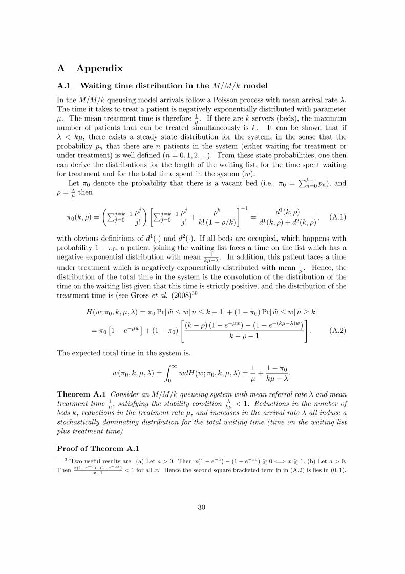
A Appendix

A.1 Waiting time distribution in the M=M=k model

In the M=M=k queueing model arrivals follow a Poisson process with mean arrival rate ¸.The time it takes to treat a patient is negatively exponentially distributed with parameter¹. The mean treatment time is therefore 1

¹ . If there are k servers (beds), the maximumnumber of patients that can be treated simultaneously is k. It can be shown that if¸ < k¹, there exists a steady state distribution for the system, in the sense that theprobability pn that there are n patients in the system (either waiting for treatment orunder treatment) is well de…ned (n = 0; 1; 2; :::). From these state probabilities, one thencan derive the distributions for the length of the waiting list, for the time spent waitingfor treatment and for the total time spent in the system (w).

Let ¼0 denote the probability that there is a vacant bed (i.e., ¼0 =Pk¡1

n=0 pn), and½ = ¸

¹ then

¼0(k; ½) =

µPj=k¡1j=0

½j

j!

¶·Pj=k¡1j=0

½j

j!+

½k

k! (1¡ ½=k)

¸¡1

=d1(k; ½)

d1(k; ½) + d2(k; ½); (A.1)

with obvious de…nitions of d1(¢) and d2(¢). If all beds are occupied, which happens withprobability 1 ¡ ¼0, a patient joining the waiting list faces a time on the list which has anegative exponential distribution with mean 1

k¹¡¸ . In addition, this patient faces a timeunder treatment which is negatively exponentially distributed with mean 1

¹ . Hence, thedistribution of the total time in the system is the convolution of the distribution of thetime on the waiting list given that this time is strictly positive, and the distribution of thetreatment time is (see Gross et al. (2008)30

H(w;¼0; k; ¹; ¸) = ¼0Pr[ ~w · wjn · k ¡ 1] + (1¡ ¼0) Pr[ ~w · wjn ¸ k]

= ¼0

£1¡ e¡¹w

¤+ (1¡ ¼0)

"(k ¡ ½) (1¡ e¡¹w)¡

¡1¡ e¡(k¹¡¸)w

¢

k ¡ ½¡ 1

#: (A.2)

The expected total time in the system is.

w(¼0; k; ¹; ¸) =

Z 1

0wdH(w;¼0; k; ¹; ¸) =

1

¹+

1¡ ¼0

k¹¡ ¸:

Theorem A.1 Consider an M=M=k queueing system with mean referral rate ¸ and meantreatment time 1

¹ , satisfying the stability condition ¸k¹ < 1. Reductions in the number of

beds k, reductions in the treatment rate ¹, and increases in the arrival rate ¸ all induce astochastically dominating distribution for the total waiting time (time on the waiting listplus treatment time)

Proof of Theorem A.130Two useful results are: (a) Let a > 0. Then x(1 ¡ e¡a) ¡ (1 ¡ e¡xa) ? 0 () x ? 1: (b) Let a > 0.

Then x(1¡e¡a)¡(1¡e¡ax)x¡1 < 1 for all x. Hence the second square bracketed term in in (A.2) is lies in (0; 1):

30

(a) We …rst show that

@H

@k=

@H

@¼0|{z}(i)

@¼0

@k|{z}(ii)

+ (1¡ ¼0)@G(w; k; ¹; ¸)

@k| {z }(iii)

> 0;

where we treat ¼0 as di¤erentiable in k to reduce notational clutter.(i) @H=@¼0 > 0.

@H

@¼0= Pr[ ~w · wjn · k ¡ 1]¡ Pr[ ~w · wjn ¸ k] =

e¡¹w ¡ e¡(k¡½)¹w

k ¡ ½¡ 1:

If k¡ ½¡ 1 > 0 the numerator and denominator are positive and if k¡ ½¡ 1 < 0 they areboth negative.

(ii) ¼0(k; ½) is increasing in k.Consider

¼0(k + 1; ½)¡ ¼0(k; ½) =d1(k + 1; ½)

d1(k + 1; ½) + d2(k + 1; ½)¡ d1(k; ½)

d1(k; ½) + d2(k; ½)

=d1(k + 1; ½)d2(k; ½)¡ d1(k; ½)d2(k + 1; ½)

[d1(k + 1; ½) + d2(k + 1; ½)] [d1(k; ½)d2(k + 1; ½)];

and so

sign [¼0(k + 1; ½)¡ ¼0(k; ½)] = sign·d1(k + 1; ½)

d1(k; ½)¡ d2(k + 1; ½)

d2(k; ½)

¸:

Nowd1(k + 1; ½)

d1(k; ½)=

Pj=kj=0

½j

j!Pj=k¡1j=0

½j

j!

> 1;

and

d2(k + 1; ½)

d2(k; ½)=

½k+1

(k + 1)! (1¡ ½=(k + 1))

k! (1¡ ½=k)

½k

=½

k + 1

(1¡ ½=k)

(1¡ ½=(k + 1))=

½

k

(k ¡ ½)

(k + 1¡ ½)< 1;

since the stability of the queueing system requires ½ < k. Hence

¼0(k + 1; ½)¡ ¼0(k; ½) > 0;

and so ¼0(k; ½) is increasing in k.(iii) G(w; k; ¹; ¸) = Pr[ ~w · wjn ¸ k] is increasing in k.The random waiting time for a patient joining the queue, conditional on there being

no empty bed, is the convolution of the distribution of two random variables: the wait for

31

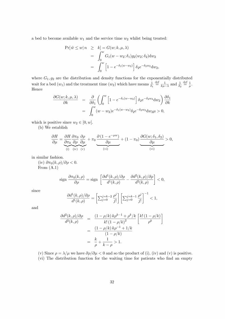
a bed to become available w1 and the service time w2 whilst being treated:

Pr[ ~w · wjn ¸ k] = G(w; k; ¹; ¸)

=

Z w

0G1(w ¡w2; ±1)g2(w2; ±2)dw2

=

Z w

0

h1¡ e¡±1(w¡w2)

i±2e

¡±2w2dw2;

where G1; g2 are the distribution and density functions for the exponentially distributed

wait for a bed (w1) and the treatment time (w2) which have means 1±1

def= 1

k¹¡¸ and 1±2

def= 1

¹ .Hence

@G(w; k; ¹; ¸)

@k=

@

@±1

µZ w

0

h1¡ e¡±1(w¡w2)

i±2e

¡±2w2dw2

¶@±1@k

=

Z w

0(w¡w2)e

¡±1(w¡w2)±2e¡±2w2dw2¹ > 0;

which is positive since w2 2 [0; w].(b) We establish

@H

@¹=

@H

@¼0|{z}(i)

@¼0

@½|{z}(iv)

@½

@¹|{z}(v)

+ ¼0@ (1¡ e¡¹w)

@¹| {z }(vi)

+ (1¡ ¼0)@G(w; ±1; ±2)

@¹| {z }(vi)

> 0;

in similar fashion.(iv) @¼0(k; ½)=@½ < 0.From (A.1)

sign@¼0(k; ½)

@½= sign

·@d1(k; ½)=@½

d1(k; ½)¡ @d2(k; ½)=@½

d2(k; ½)

¸< 0;

since@d1(k; ½)=@½

d1(k; ½)=

·Pj=k¡2j=0

½j

j!

¸·Pj=k¡1j=0

½j

j!

¸¡1

< 1;

and

@d2(k; ½)=@½

d2(k; ½)=

(1¡ ½=k) k½k¡1 + ½k=k

k! (1¡ ½=k)2

·k! (1¡ ½=k)

½k

¸

=(1¡ ½=k) k½¡1 + 1=k

(1¡ ½=k)

=k

½+

1

k ¡ ½> 1:

(v) Since ½ = ¸=¹ we have @½=@¹ < 0 and so the product of (i), (iv) and (v) is positive.(vi) The distribution function for the waiting time for patients who …nd an empty

32

queue is decreasing in ¹@(1¡ e¡¹w1)

@¹= w1e

¡¹w1 > 0:

(vi) @G(w; k; ¹; ¸)=@¹ > 0.¹ a¤ects both ±1 = k¹¡ ¸ and ±2 = ¹ and so

@G(w; ±1; ±2)

@¹=

@G(w; ±1; ±2)

@±1

@±1@¹

+@G(w; ±1; ±2)

@±2

@±2@¹

=@

@±1

µZ w

0G1(w ¡w2; ±1)g2(w2; ±2)dw2

¶k

+@

@±2

µZ w

0g1(w1; ±1)G2(w ¡w1; ±2)dw1

¶

=

Z w

0(w ¡w2)e¡¸1(w¡w2)¸2e

¡¸2w2dw2k

+

Z w

0¸1e

¡¸1w1(w ¡w1)e¡¸2(w¡w1)dw1 > 0 :

(c) Finally, we show

@H

@¸=

@H

@¼0|{z}(i)

@¼0

@½|{z}(iv)

@½

@¸|{z}(vii)

+ (1¡ ¼0)@G(w; ±1; ±2)

@¸| {z }(viii)

< 0:

(vii) Since (i) is positive, (iv) is negative, and (viii) is positive because ½ = ¸=¹, the …rstterm in @H=@¸ is negative. (viii) is

@G(w; ±1; ±2)

@¸=

@

@±1

µZ w

0

h1¡ e¡±1(w¡w2)

i±2e

¡±2w2dw2

¶@±1@¸

= ¡Z w

0(w¡w2)e

¡±1(w¡w2)±2e¡±2w2dw2 < 0;

which completes the proof of Proposition A1.¥

A.2 Equilibrium mean waiting time

Lemma A.1 Increases in supply conditions that are accompanied by a quality reduction tokeep demand (expected wait) constant lower the expected wait (increase expected demand).

Proof of Lemma A.1

dwe(q; k; ¹)

ds

¯¯d¸=0

= ¹ws + ¹w¸¸s ¡ ¹w¸¸q¸s¸q

= ¹ws < 0 (s = k; ¹),

d¸ds

¯¯d ¹w=0

= ¸s ¡ ¸q¹wes

¹weq

= ¸s ¡ ¸q( ¹ws + ¹w¸¸s)

¹w¸¸q= ¡ ¹ws

¹w¸> 0 (s = k; ¹).

Proof of Proposition 2 (a) Linear (LN) preferences. De…ne utility if ill and treated inthe public hospital after a wait of w as u(y; q; w) = t1(y; q)¡t2(y; q)w so that expected util-

33

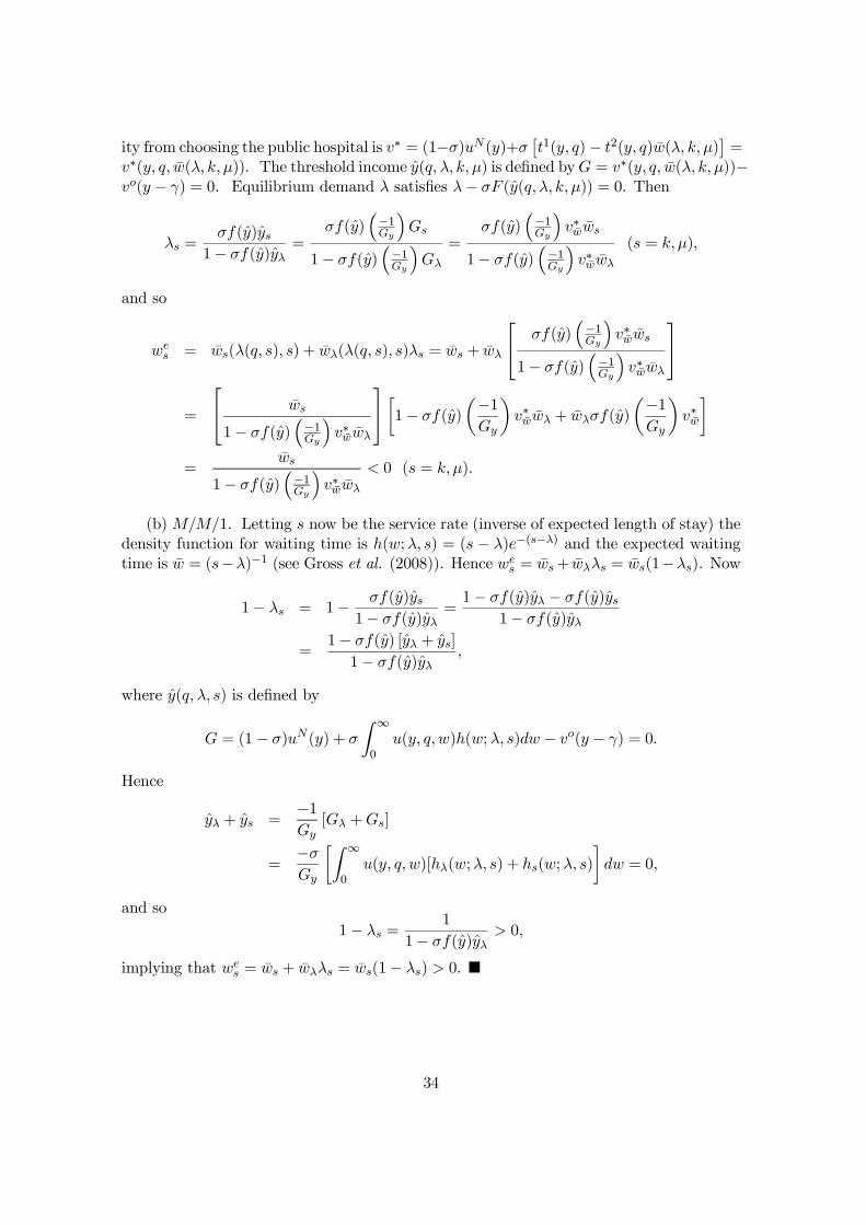
ity from choosing the public hospital is v¤ = (1¡¾)uN(y)+¾£t1(y; q)¡ t2(y; q) ¹w(¸; k; ¹)

¤=

v¤(y; q; ¹w(¸; k; ¹)). The threshold income y(q; ¸; k; ¹) is de…ned byG = v¤(y; q; ¹w(¸; k; ¹))¡vo(y ¡ °) = 0. Equilibrium demand ¸ satis…es ¸¡ ¾F (y(q; ¸; k; ¹)) = 0. Then

¸s =¾f(y)ys

1¡ ¾f(y)y¸=

¾f(y)³¡1Gy

´Gs

1¡ ¾f(y)³¡1Gy

´G¸

=¾f(y)

³¡1Gy

´v¤¹w ¹ws

1¡ ¾f(y)³¡1Gy

´v¤¹w ¹w¸

(s = k; ¹);

and so

wes = ¹ws(¸(q; s); s) + ¹w¸(¸(q; s); s)¸s = ¹ws + ¹w¸

24

¾f(y)³¡1Gy

´v¤¹w ¹ws

1¡ ¾f(y)³¡1Gy

´v¤¹w ¹w¸

35

=

24 ¹ws

1¡ ¾f(y)³¡1Gy

´v¤¹w ¹w¸

35·1¡ ¾f(y)

µ¡1

Gy

¶v¤¹w ¹w¸ + ¹w¸¾f(y)

µ¡1

Gy

¶v¤¹w

¸

=¹ws

1¡ ¾f(y)³¡1Gy

´v¤¹w ¹w¸

< 0 (s = k; ¹):

(b) M=M=1: Letting s now be the service rate (inverse of expected length of stay) thedensity function for waiting time is h(w;¸; s) = (s ¡ ¸)e¡(s¡¸) and the expected waitingtime is ¹w = (s¡¸)¡1 (see Gross et al. (2008)). Hence we

s = ¹ws+ ¹w¸¸s = ¹ws(1¡¸s). Now

1¡ ¸s = 1¡ ¾f(y)ys1¡ ¾f(y)y¸

=1¡ ¾f(y)y¸ ¡ ¾f(y)ys

1¡ ¾f(y)y¸

=1¡ ¾f(y) [y¸ + ys]

1¡ ¾f(y)y¸;

where y(q; ¸; s) is de…ned by

G = (1¡ ¾)uN(y) + ¾

Z 1

0u(y; q;w)h(w;¸; s)dw ¡ vo(y ¡ °) = 0:

Hence

y¸ + ys =¡1

Gy[G¸ +Gs]

=¡¾

Gy

·Z 1

0u(y; q; w)[h¸(w;¸; s) + hs(w;¸; s)

¸dw = 0;

and so1¡ ¸s =

1

1¡ ¾f(y)y¸> 0;

implying that wes = ¹ws + ¹w¸¸s = ¹ws(1¡ ¸s) > 0. ¥

34

A.3 Demand constant welfare changes

Theorem A.2 In equilibrium an increase in hospital attribute z (= q; ¹; k) accompaniedby an adjustment in hospital attribute x (x = q; ¹; k; x 6= z) to keep demand constant hasno e¤ect on patient welfare Be(q; ¹; k) if and only if

(a) patient preferences are quasi-separable between quality and waiting time :

v = ¾

½Z[a1(y) + a2(y)r(q;w)]dH(w;¸; k; ¹)

¾+ (1¡ ¾)uN(y)

= ¾£a1(y) + a2(y)R(q; ¸; k; ¹)

¤+ (1¡ ¾)uN(y);

and (b) the welfare function respects patient preferences over quality and waiting time

be(y; q; k; ¹) = ¾[m0(y) +m1(y)m2(R(q; k; ¹))] + (1¡ ¾)mN(y); m2R > 0:

Proof of Theorem A.2. In equilibrium an increase in hospital attribute z accompaniedby an adjustment in hospital attribute x to keep demand constant changes patient welfareat the rate

Bez(q; ¹; k)¡Be

x(q; ¹; k)¸z(q; ¹; k)

¸x(q; ¹; k)

From (15) and Lemma 1 in the main text:

Bez ¡Be

x

¸z¸x

=

Z ye(q;;¹;k)

ymin

·bez ¡ bex

¸z¸x

¸dF (y)

+ [be(y; q; k; ¹)¡ bo(y ¡ °; qo)]¾f (ye)

·yez ¡ yex

¸z¸x

¸

=

Z ye(q;¹;k)

ymin

·bez ¡ bex

¸z¸x

¸dF (y)

=

Z y(q;¸;¹;k)

ymin

·bz(y; q; ¸; k; ¹) + b¸¸z ¡ bx(y; q; ¸; k; ¹)

¸z¸x

¡ b¸¸x¸z¸x

¸dF (y)

=

Z y(q;¸;¹;k)

ymin

·bz(y; q; ¸; k; ¹)¡ bx(y; q; ¸; k; ¹)

¸z¸x

¸dF (y)

= Bz(y; q; ¸; ¹; k)¡Bx(y; q; ¸; ¹; k)vz(y; q; ¸; ¹; k)

vx(y; q; ¸; ¹; k)= T (y; q; ¸; ¹; k): (A.3)

For T (y; q; ¸; ¹; k) = 0 to hold for all the equilibria generated by the premium for privatehealth care °, which a¤ects (A.3) only via the the threshold income y, requires

@T

@y=

·bz(y; q; ¸; ¹; k)¡ bx(y; q; ¸; ¹; k)

vz(y; q; ¸; ¹; k)

vx(y; q; ¸; ¹; k)

¸f (y)

¡Bx1

v2x[vzyvx ¡ vzvxy] = 0 (A.4)

This holds in general (i.e., for all distributions of income) only if both square bracketedterms are zero. The …rst term is zero only if the marginal rate of substitution between

35

z and x for a patient of given income are the same for the regulator and the patient.The second is zero only if the patient marginal rate of substitution between z and x isuna¤ected by patient income. Su¢ciency of (a) and (b) is easily established.¥

Theorem A.3 The e¤ect on social bene…t of an increase in hospital attribute z followedby an adjustment in attribute x to keep demand constant is given by

Bez ¡Be

x

¸z¸x

=

Z by

ymin

bx

·bz(y; ¢)bx(y; ¢)

¡ vz(by; ¢)vx(by; ¢)

¸dF (y) (A.5)

=

Z by

ymin

bz

264

0@@ log bz(y;¢)

by(y;¢)@y

¡@ log bx(y;¢)

by(y;¢)@y

1Aey2[y;by]

(y ¡ by) +µbz(by; ¢)bx(by; ¢)

¡ vz(by; ¢)vx(by; ¢)

¶375 dF (y):

(A.6)

The theorem implies that when individual preferences are respected, so that the secondround bracket term is zero, then Be

z ¡ Bex¸z¸x

> 0(< 0) if the marginal willingness to payfor attribute x increases faster (slower) with income than that for attribute z. Underquasi-separable individual and social preferences ((3) and (16)), bz(y;¢)

bx(y;¢) = vz(by;¢)vx(by;¢) = Rz(¢)

Rx(¢)and Be

z ¡Bex¸z¸x

= 0. Under speci…c egalitarianism, bz(y;¢)bx(y;¢) is independent of income, and

the sign of (A.5) is the sign of bz(by;¢)bx(by;¢) ¡

vz(by;¢)vx(by;¢) .

Proof of Theorem A.3.We have, making use of the mean value theorem in the third line

Bez ¡Be

x

¸z¸x

=

Z by

ymin

·bez(y; q; k; ¹)¡ bex(y; q; k; ¹)

¸z¸x

¸dF (y)

=

Z by

ymin

bx

·bz(y; q; ¸; k; ¹)

bx(y; q; ¸; k; ¹)¡ bz(by; q; ¸; k; ¹)

bx(by; q; ¸; k; ¹)+

bz(by; q; ¸; k; ¹)bx(by; q; ¸; k; ¹)

¡ ¸z¸x

¸dF (y)

=

Z by

ymin

bx(y; ¢)

264(y ¡ by)

@ bz(~y;¢)bx(~y;¢)@y

¯¯¯ey2[y;by]

+bz(by; ¢)bx(by; ¢)

¡ vz(by; ¢)vx(by; ¢)

375dF (y)

De…ne

¢(by; ¢) def=

bz(by; ¢)bx(by; ¢)

¡ vz(by; ¢)vx(by; ¢)

Bez ¡Be

x

¸z¸x

=

Z by

ymin

bx(y; ¢)

264(y ¡ by)

@ bz(~y;¢)bx(~y;¢)@y

¯¯¯ey2[y;by]

+¢(by; ¢)

375dF (y)

=

Z by

ymin

bx(y; ¢)

264(y ¡ by)

0B@bz(~y; ¢)bx(~y; ¢)

@ log bz(~y;¢)bx(¹y;¢)

@y

¯¯¯ey2[y;by]

1CA+¢(by; ¢)

375dF (y)

36

If patient preferences are respected ¢(by; ¢) = 0 then

Bez ¡Be

x

¸z¸x

=

Z by

ymin

vx(y; ¢)

264(y ¡ by)

0B@bz(~y; ¢)bx(~y; ¢)

0@@ log vz(y;¢)

vy(y;¢)@y

¡@ log vx(y;¢)

vy(y;¢)@y

1A¯¯¯ey2[y;by]

1CA

375dF (y)

=

Z by

ymin

vx(y; ¢)"(y ¡ by)

Ãbz(~y; ¢)bx(~y; ¢)

µ@ logMWPz(~y; ¢)

@y¡ @ logMWPx(~y; ¢)

@y

¶¯¯ey2[y;by]

!#dF (y)

¥

A.4 Demand constant change in insurance cost

Lemma A.2 The change in equilibrium insurance costs when supply s (s = k; ¹) is in-creased and q is reduced to keep demand constant is

dcIe

ds

¯¯d¸=0

= cIes ¡ cIeq¸s¸q

= ¾ ¹ws

Z ye

ymin

ydF (y) < 0; (s = k; ¹). (A.7)

The change in equilibrium insurance costs when quality is increased and supply s (s = k; ¹)is reduced to keep demand constant is

dcIe

dq

¯¯d¸=0

= cIeq ¡ cIes¸q¸s

= ¡¾ ¹ws¸q¸s

Z ye

ymin

ydF (y) > 0 (s = k; ¹). (A.8)

Proof of Lemma A.2

cIez ¡ cIex¸z¸x

= ¾

µwez ¡we

x

¸z¸x

¶Z y

ymin

ydF (y) + ¾w

Z y

ymin

ydF (y)yf(y)

µyez ¡ yex

¸z¸x

¶

= ¾

µwz ¡wx

¸z¸x

¶Z y

ymin

ydF (y) + ¾w

Z y

ymin

ydF (y)yf(y)

µyz ¡ yx

¸z¸x

¶

= ¾

µwz ¡wx

¸z¸x

¶Z y

ymin

ydF (y)

since the second round bracketed term in the second line is zero (cf (10)). ¥

A.5 Derivation of optimal pricing rules

Proof of Proposition 3 The hospital maximises (23), leading to decisions q(p¸; pk; p¹);k(p¸; pk; p¹); ¹(p¸; pk; p¹) satisfying (24). The regulation problem is

maxp¸;pk;p¹

Be(q; k; ¹)¡ (1 + µ)[p¸¸(q; k; ¹) + pkk + p¹¹+ T + cIe(q; k; ¹)]:

T is set to leave the hospital with no …nancial rent

T = ¡p¸¸¡ pkk ¡ p¹¹+ cHe(q; k; ¹);

37

and so the regulator problem is equivalently

maxp¸;pk;p¹

Be(q(p¸; pk; p¹); k(p¸; pk; p¹); ¹(p¸; pk; p¹))

¡(1 + µ)cHe(q(p¸; pk; p¹); k(p¸; pk; p¹); ¹(p¸; pk; p¹))

¡(1 + µ)cIe(q(p¸; pk; p¹); k(p¸; pk; p¹); ¹(p¸; pk; p¹))

The FOCs to this regulation problem can be written as0B@

@q@p¸

@k@p¸

@¹@p¸

@q@pk

@k@pk

@¹@pk

@q@p¹

@k@p¹

@¹@p¹

1CA

0@

Beq ¡ (1 + µ)[cHe

q + cIeq ]Bek ¡ (1 + µ)[cHe

k + cIek ]Be¹ ¡ (1 + µ)[cHe

¹ + cIe¹ ]

1A =

0@

000

1A :

But making use of the hospital FOCs, the regulator’s FOCs can be written as0B@

@q@p¸

@k@p¸

@¹@p¸

@q@pk

@k@pk

@¹@pk

@q@p¹

@k@p¹

@¹@p¹

1CA

240@

Seq

Sek

Se¹

1A¡

0@

¸q 0 0¸k 1 0¸¹ 0 1

1A0@

pFB¤¸

pFB¤k

pFB¤¹

1A35 =

0@

000

1A :

where Sez = ¯Be

z ¡ cIez where ¯ = [1¡ ®(1 + µ)]=(1 + µ).The (3£ 3) matrix of price e¤ects is invertible. Hence, the FB optimal prices are

0@

pFB¤¸

pFB¤k

pFB¤¹

1A =

0@

¸q 0 0¸k 1 0¸¹ 0 1

1A

¡10@

Seq

Sek

Se¹

1A =

0B@

1¸q

0 0

¡¸k¸q

1 0

¡¸¹¸q

0 1

1CA

0@

Seq

Sek

Se¹

1A

=

0BB@

Seq¸q

Sek ¡ ¸k

¸qSeq

Sek ¡

¸¹¸qSeq

1CCA :¥

Proof of Proposition 4 The generic …rst order condition for the hospital facing pricesp¸; pk and pq is

p¸¸z + pk1(z=k) + pq1(z=q) + ®Bez = cHe

z (z = q; k; ¹):

The …rst order conditions for the regulator’s problem is0B@

@q@p¸

@k@p¸

@¹@p¸

@q@pk

@k@pk

@¹@pk

@q@pq

@k@pq

@¹@pq

1CA

0@

Beq ¡ (1 + µ)[cHe

q + cIeq ]

Bek ¡ (1 + µ)[cHe

k + cIek ]Be¹ ¡ (1 + µ)[cHe

¹ + cIe¹ ]

1A =

0@

000

1A :

Replacing cHez by the LHS of the hospital’s …rst order condition shows that

Bez ¡ (1 + µ)[cHe

z + cIez ] = (1 + µ)£Sez ¡ p¸¸z ¡ pk1(z=k) ¡ pq1(z=q)

¤;

38

which allows us to rewrite the regulator’s FOCs as0B@

@q@p¸

@k@p¸

@¹@p¸

@q@pk

@k@pk

@¹@pk

@q@pq

@k@pq

@¹@pq

1CA

240@

Seq

Sek

Se¹

1A¡

0@

¸q 0 1¸k 1 0¸¹ 0 0

1A0@

pFB¤¤¸

pFB¤¤k

pFB¤¤¹

1A35 =

0@

000

1A :

Since the (3£ 3) response matrix is invertible, the FOCs are equivalent to the squarebracket vector being zero. Hence

0@

pFB¤¤¸

pFB¤¤k

pFB¤¤¹

1A =

0@

¸q 0 1¸k 1 0¸¹ 0 0

1A

¡10@

Seq

Sek

Se¹

1A =

0B@

0 0 1¸¹

0 1 ¡¸k¸¹

1 0 ¡ ¸q¸¹

1CA

0@

Seq

Sek

Se¹

1A ;

=

0BB@

Se¹¸¹

Sek ¡ ¸k

¸¹Se¹

Seq ¡ ¸q

¸¹Se¹

1CCA =

0B@

Se¹¸¹

Sek ¡ ¸kp

FB¤¤¸

Seq ¡ ¸qp

FB¤¤¸

1CA :¥

Proof of Proposition 5 The hospital choices q(p¸; pk; pw); k(p¸; pk; pw); ¹(p¸; pk; pw)satisfy (24). The regulation problem is then

maxp¸;pk;pw

Be(q(p¸; pk; pw); k(p¸; pk; pw); ¹(p¸; pk; pw))

¡(1 + µ)cHe(q(p¸; pk; pw); k(p¸; pk; pw); ¹(p¸; pk; pw))

¡(1 + µ)cIe(q(p¸; pk; pw); k(p¸; pk; pw); ¹(p¸; pk; pw)):

The FOCs for welfare maximisation are0B@

@q@p¸

@k@p¸

@¹@p¸

@q@pk

@k@pk

@¹@pk

@q@pw

@k@pw

@¹@pw

1CA

0@

Beq ¡ (1 + µ)[cHe

q + cIeq ]Bek ¡ (1 + µ)[cHe

k + cIek ]Be¹ ¡ (1 + µ)[cHe

¹ + cIe¹ ]

1A =

0@

000

1A :

By making use of the hospital FOCs, the regulator’s FOCs can be written as0B@

@q@p¸

@k@p¸

@¹@p¸

@q@pk

@k@pk

@¹@pk

@q@pw

@k@pw

@¹@pw

1CA

240@

Seq

Sek

Se¹

1A¡

0@

¸q weq 0

¸k wek 1

¸¹ we¹ 0

1A0@

pFB+¸

pFB+w

pFB+k

1A35 =

0@

000

1A : (A.9)

The (3£ 3) matrix of price e¤ects is invertible. Hence, under FB, the optimal pricesare obtained by setting the square bracket term to zero and solving for the prices:

0@

pFB+¸

pFB+w

pFB+k

1A =

0BB@

we¹

¸qwe¹¡¸¹we

q0 ¡ we

q

¸qwe¹¡¸¹we

q

¡ ¸¹¸qwe

¹¡¸¹weq

0 ¸q¸qwe

¹¡¸¹weq

¡¸kwe¹¡¸¹we

k¸qwe

¹¡¸¹weq

1¸kw

eq¡¸qwe

k¸qwe

¹¡¸¹weq

1CCA

0@

Seq

Sek

Se¹

1A :

39

Using (13)-(14), and Sez = Sz + S¸¸z, this reduces to

0@

pFB+¸

pFB+w

pFB+k

1A =

0BB@

Seq¸q

¡ (S¹ ¡ Sq¸¹¸q)w¸w¹

(S¹ ¡ Sq¸¹¸q) 1w¹

(Sk ¡ Sq¸k¸q)¡ (S¹ ¡ Sq

¸¹¸q

)wkw¹

1CCA ;

which gives (29)-(31). ¥

Proof of Proposition 6 When k cannot be priced, the regulator’s FOCs (A.9) on p¸and pw are

Ã@q@p¸

@k@p¸

@¹@p¸

@q@pw

@k@pw

@¹@pw

!240@

Seq

Sek

Se¹

1A¡

0@

¸q weq 0

¸k wek 1

¸¹ we¹ 0

1A0@

p¸pw0

1A35 =

µ00

¶:

Use (A.9) to replace

0@

Seq

Sek

Se¹

1A by

0@

¸q weq 0

¸k wek 1

¸¹ we¹ 0

1A0@

pFB++¸

pFB++w

pFB++k

1A, and let ++ indicate that

prices are evaluated at the SB values for q; ¹; k. Then

µ00

¶=

Ã@q@p¸

@k@p¸

@¹@p¸

@q@pw

@k@pw

@¹@pw

!240@

¸q weq 0

¸k wek 1

¸¹ we¹ 0

1A0@

pFB++¸

pFB++w

pFB++k

1A

¡

0@

¸q weq 0

¸k wek 1

¸¹ we¹ 0

1A0@

pSB¸pSBw0

1A35

This system of equations will hold in two distinct cases.(i) the FB price for k is zero. This is the case discussed in section 4.2. In that case

the square bracket term is the zero vector when also pSB¸ = pFB¸ and pSBw = pFB

w (the(3£ 3) matrix being invertible).

(ii) when the FB price for k is di¤erent from zero. Then the (3 £ 1) square bracketvector should be orthogonal to the two row vectors of responses w.r.t. the prices p¸ andpw. This is equivalent to

Ã@q@p¸

@k@p¸

@¹@p¸

@q@pw

@k@pw

@¹@pw

!0@

¸q weq 0

¸k wek 1

¸¹ we¹ 0

1A0@

pFB++¸

pFB++w

pFB++k

1A

=

Ã@q@p¸

@k@p¸

@¹@p¸

@q@pw

@k@pw

@¹@pw

!0@

¸q weq 0

¸k wek 1

¸¹ we¹ 0

1A0@

pSB¸pSBw0

1A :

Using the de…nitions @¸¤@pi

def=P

z=q;k;¹ ¸z@z@pi

(i = ¸;w) and @we¤@pi

def=P

z=q;k;¹wez@z@pi

(i =¸;w) (i.e., the optimal demand and expected wait responses that follows from the optimal

40

responses in q; k; ¹) gives:

Ã@¸¤@p¸

@we¤@p¸

@k@p¸

@¸¤@pw

@we¤@pw

@k@pw

!0@

pFB++¸pFB++w

pFB++k

1A =

Ã@¸¤@p¸

@we¤@p¸

@¸¤@pw

@we¤@pw

!µpSB¸pSBw

¶

implying

µpSB¸pSBw

¶=

Ã@¸¤@p¸

@we¤@p¸

@¸¤@pw

@we¤@pw

!¡1à @¸¤@p¸

@we¤@p¸

@k@p¸

@¸¤@pw

@we¤@pw

@k@pw

!0@

pFB++¸pFB++w

pFB++k

1A

=

µpFB++¸

pFB++w

¶+

Ã@¸¤@p¸

@we¤@p¸

@¸¤@pw

@we¤@pw

!¡1Ã @k@p¸@k@pw

!pFB++k

=

µpFB++¸

pFB++w

¶+

1@¸¤@p¸

@we¤@pw

¡ @¸¤@pw

@we¤@p¸

Ã@we¤@pw

¡@we¤@p¸

¡ @¸¤@pw

@¸¤@p¸

!Ã@k@p¸@k@pw

!pFB++k :

Then we obtain the following SB pricing rules:

pSB¸ = pFB++¸ +

@we¤@pw

@k@p¸

¡ @k@pw

@we¤@p¸

@¸¤@p¸

@we¤@pw

¡ @¸¤@pw

@we¤@p¸

pFB++k ;

pSBw = pFB++w +

¡ @¸¤@pw

@k@p¸

+ @¸¤@p¸

@k@pw

@¸¤@p¸

@we¤@pw

¡ @¸¤@pw

@we¤@p¸

pFB++k ;

which upon using the de…nitions (33)-(34) can be written as (35)-(36). ¥

Proof of Proposition 7 Using (29)-(31), the requirement for pFB+k = 0 amounts to

pFB+k = Se

k ¡ pFB+¸ ¸k ¡ pFB+

w wk

= Sek ¡ Se

q

¸k¸q

¡µSe¹ ¡ Se

q

¸¹¸q

¶wk

w¹= 0:

Expanding by using the de…nition S = ¯B ¡ cI gives

¯

µBk ¡Bq

¸k¸q

¶¡ ¯

µB¹ ¡Bq

¸¹¸q

¶wk

w¹

= cIk ¡ cIq¸k¸q

¡µcI¹ ¡ cIq

¸¹¸q

¶wk

w¹:

41

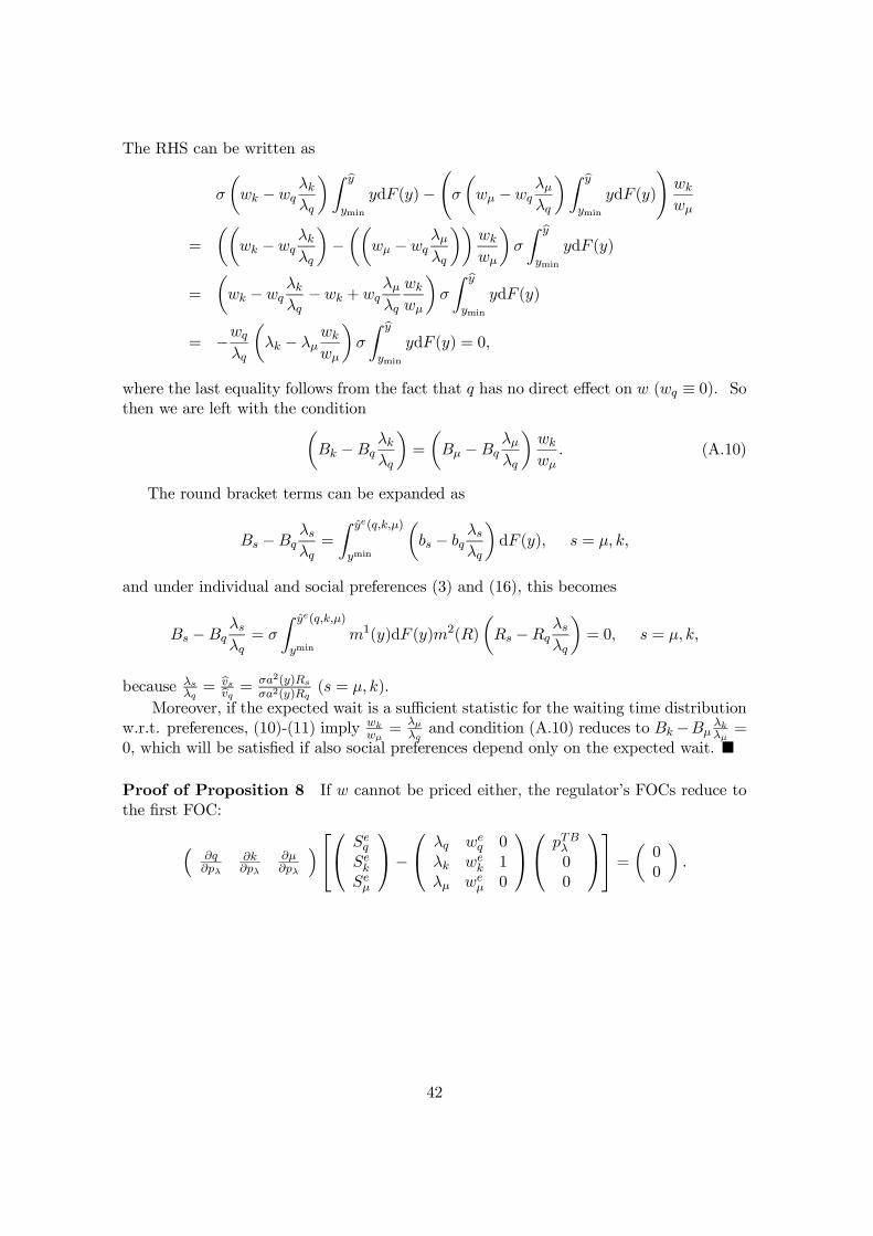
The RHS can be written as

¾

µwk ¡wq

¸k¸q

¶Z by

ymin

ydF (y)¡Ã¾

µw¹ ¡wq

¸¹¸q

¶Z by

ymin

ydF (y)

!wk

w¹

=

µµwk ¡wq

¸k¸q

¶¡µµ

w¹ ¡wq¸¹¸q

¶¶wk

w¹

¶¾

Z by

ymin

ydF (y)

=

µwk ¡wq

¸k¸q

¡wk +wq¸¹¸q

wk

w¹

¶¾

Z by

ymin

ydF (y)

= ¡wq

¸q

µ¸k ¡ ¸¹

wk

w¹

¶¾

Z by

ymin

ydF (y) = 0;

where the last equality follows from the fact that q has no direct e¤ect on w (wq ´ 0). Sothen we are left with the condition

µBk ¡Bq

¸k¸q

¶=

µB¹ ¡Bq

¸¹¸q

¶wk

w¹: (A.10)

The round bracket terms can be expanded as

Bs ¡Bq¸s¸q

=

Z ye(q;k;¹)

ymin

µbs ¡ bq

¸s¸q

¶dF (y); s = ¹; k;

and under individual and social preferences (3) and (16), this becomes

Bs ¡Bq¸s¸q

= ¾

Z ye(q;k;¹)

ymin

m1(y)dF (y)m2(R)

µRs ¡Rq

¸s¸q

¶= 0; s = ¹; k;

because ¸s¸q

= bvsbvq = ¾a2(y)Rs

¾a2(y)Rq(s = ¹; k).

Moreover, if the expected wait is a su¢cient statistic for the waiting time distributionw.r.t. preferences, (10)-(11) imply wk

w¹= ¸¹

¸qand condition (A.10) reduces to Bk¡B¹

¸k¸¹

=0, which will be satis…ed if also social preferences depend only on the expected wait. ¥

Proof of Proposition 8 If w cannot be priced either, the regulator’s FOCs reduce tothe …rst FOC:

³@q@p¸

@k@p¸

@¹@p¸

´240@

Seq

Sek

Se¹

1A¡

0@

¸q weq 0

¸k wek 1

¸¹ we¹ 0

1A0@

pTB¸00

1A35 =

µ00

¶:

42

Use (A.9) to replace

0@

Seq

Sek

Se¹

1A by

0@

¸q weq 0

¸k wek 1

¸¹ we¹ 0

1A0@

pFB+++¸

pFB+++w

pFB+++k

1A, +++ indicating that

prices are evaluated at the TB values for q; ¹; k. Then

³@q@p¸

@k@p¸

@¹@p¸

´240@

¸q weq 0

¸k wek 1

¸¹ we¹ 0

1A0@

pFB+++¸pFB+++w

pFB+++k

1A¡

0@

¸q weq 0

¸k wek 1

¸¹ we¹ 0

1A0@

pTB¸00

1A35 = 0:

Assuming that (pFB+++w ; pFB+++

k ) 6= (0; 0), and using the de…nitions of @¸¤@p¸

and @we¤@p¸

gives

³@¸¤@p¸

@we¤@p¸

@k@p¸

´0@

pFB+++¸

pFB+++w

pFB+++k

1A =

@¸¤

@p¸pTB¸

+

pTB¸ = pFB+++¸ +

@we¤@p¸@¸¤@p¸

pFB+++w +

@k@p¸@¸¤@p¸

pFB+++k :

Using the de…nitions in (37), this can be rewritten as (38). ¥

Proof of Proposition 9 From (38) the third best output price will coincide with its…rst best value when both pFB+

w = 0 and pFB+k = 0. Using (29), the condition that

pFB+w = 0 is equivalent to

¯

µB¹ ¡Bq

¸¹¸q

¶=

µcI¹ ¡ cIq

¸¹¸q

¶;

= ¾w¹

Z by

ymin

ydF;

which will only hold when preferences are quasi-separable and insurance costs are absentsuch that both sides of the expression equal zero. The condition that pFB+

k = 0 thenreduces to (see (31))

¯

µBk ¡Bq

¸k¸q

¶=

µcIk ¡ cIq

¸¹¸q

¶

= ¾wk

Z by

ymin

ydF;

which also holds under the same conditions. ¥

Proof of Proposition 10 The proof consists of three parts. In the …rst part, we derivethe …rst best pricing and cost-sharing rules. The second part then derives the second-bestrules (giving (39)). The last part derives the third-best rules (giving (40)).

(a) We …rst solve for the …rst best pricing/cost-sharing scheme. When the hospital

43

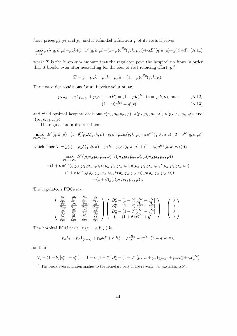
faces prices p¸; pk and pw and is refunded a fraction ' of its costs it solves

maxq;k;¹

p¸¸(q; k; ¹)+pkk+pwwe(q; k; ¹)¡(1¡')cHe(q; k; ¹; t)+®Be(q; k; ¹)¡g(t)+T; (A.11)

where T is the lump sum amount that the regulator pays the hospital up front in orderthat it breaks even after accounting for the cost of cost-reducing e¤ort, g:31

T = g ¡ p¸¸¡ pkk ¡ p¹¹+ (1¡ ')cHe(q; k; ¹):

The …rst order conditions for an interior solution are

p¸¸z + pk1(z=k) + pwwez + ®Be

z = (1¡ ')cHez (z = q; k; ¹), and (A.12)

¡(1¡ ')cHet = g0(t): (A.13)

and yield optimal hospital decisions q(p¸; pk; pw; '); k(p¸; pk; pw; '); ¹(p¸; pk; pw; '); andt(p¸; pk; pw; ').

The regulation problem is then

maxp¸;pk;pw

Be(q; k; ¹)¡(1+µ)[p¸¸(q; k; ¹)+pkk+pww(q; k; ¹)+'cHe(q; k; ¹; t)+T+cIe(q; k; ¹)]

which since T = g(t)¡ p¸¸(q; k; ¹)¡ pkk ¡ pww(q; k; ¹) + (1¡ ')cHe(q; k; ¹; t) is

maxp¸;pk;pw

Be(q(p¸; pk; pw; '); k(p¸; pk; pw; '); ¹(p¸; pk; pw; '))

¡(1 + µ)cHe(q(p¸; pk; pw; '); k(p¸; pk; pw; '); ¹(p¸; pk; pw; '); t(p¸; pk; pw; '))

¡(1 + µ)cIe(q(p¸; pk; pw; '); k(p¸; pk; pw; '); ¹(p¸; pk; pw; '))

¡(1 + µ)g(t(p¸; pk; pw; ')):

The regulator’s FOCs are

0BBB@

@q@p¸

@k@p¸

@¹@p¸

@t@p¸

@q@pw

@k@pw

@¹@pw

@t@pw

@q@'

@k@'

@¹@'

@t@'

@q@pk

@k@pk

@¹@pk

@t@pk

1CCCA

0BB@

Beq ¡ (1 + µ)[cHe

q + cIeq ]

Bek ¡ (1 + µ)[cHe

k + cIek ]Be¹ ¡ (1 + µ)[cHe

¹ + cIe¹ ]0¡ (1 + µ)[cHe

t + g0]

1CCA =

0BB@

0000

1CCA :

The hospital FOC w.r.t. z (z = q; k; ¹) is

p¸¸z + pk1(z=k) + pwwez + ®Be

z + 'cHeZ = cHe

z (z = q; k; ¹);

so that

Bez ¡ (1 + µ)[cHe

z + cIez ] = [1¡ ® (1 + µ)]Bez ¡ (1 + µ)

¡p¸¸z + pk1(z=k) + pww

ez + 'cHe

z

¢

31The break-even condition applies to the monetary part of the revenue, i.e., excluding ®Be.

44

or equivalently

Bez

1 + µ¡ [cHe

z + cIez ] = ¯Bez ¡

¡p¸¸z + pk1(z=k) + pww

ez + 'cHe

z

¢¡ cIez .

Then the regulator’s FOCs can be written as (since Se' = 0)

0BBB@

@q@p¸

@k@p¸

@¹@p¸

@t@p¸

@q@pw

@k@pw

@¹@pw

@t@pw

@q@'

@k@'

@¹@'

@t@'

@q@pk

@k@pk

@¹@pk

@t@pk

1CCCA

2664

0BB@

Seq

Sek

Se¹

0

1CCA¡

0BB@

¸q weq cHe

q 0¸k we

k cHek 1

¸¹ we¹ cHe

¹ 00 0 cHe

t 0

1CCA

0BB@

pFBcs¸

pFBcsw

'FBcs

pFBcsk

1CCA

3775 =

0BB@

0000

1CCA :

Since the (4£ 4) matrix of responses is invertible, these FOCs are equivalent to

0BB@

pFBcs¸

pFBcsw

'FBcs

pFBcsk

1CCA =

0BB@

¸q weq cHe

q 0¸k we

k cHek 1

¸¹ we¹ cHe

¹ 00 0 cHe

t 0

1CCA

¡10BB@

Seq

Sek

Se¹

0

1CCA (A.14)

=

0BBBB@

we¹

¸qwe¹¡¸¹we

q0 ¡ we

q

¸qwe¹¡¸¹we

q

¡ ¸¹¸qwe

¹¡¸¹weq

0¸q

¸qwe¹¡¸¹we

q

0 0 0

¡¸kwe¹¡¸¹we

k¸qwe

¹¡¸¹weq

1¸kw

eq¡¸qwe

k¸qwe

¹¡¸¹weq

1CCCCA

0@

Seq

Sek

Se¹

1A ;

which gives 'FBcs = 0 (and therefore (pFBcs¸ ; pFBcs

w ; pFBcsk ) as derived earlier in Proposition

5).(b) When beds can no longer be rewarded, the regulator has three instruments: p¸; pw

and '. The hospital’s objective function reduces to

p¸¸(q; k; ¹) + pwwe(q; k; ¹) + ®Be(q; k; ¹)¡ (1¡ ')cHe(q; k; ¹)

and in (A.12) the term pk1(z=k) is absent.When k cannot be priced, the regulator’s FOCs reduce to the …rst three rows:

0B@

@q@p¸

@k@p¸

@¹@p¸

@t@p¸

@q@pw

@k@pw

@¹@pw

@t@pw

@q@'

@k@'

@¹@'

@t@'

1CA

2664

0BB@

Seq

Sek

Se¹

0

1CCA¡

0BB@

¸q weq cHe

q 0¸k we

k cHek 1

¸¹ we¹ cHe

¹ 0

0 0 cHet 0

1CCA

0BB@

pSBcs¸

pSBcsw

'SBcs

0

1CCA

3775 =

0@

000

1A :

We can then use (A.14) to replace

0BB@

Seq

Sek

Se¹

0

1CCA by

0BB@

¸q weq cHe

q 0¸k we

k cHek 1

¸¹ we¹ cHe

¹ 00 0 cHe

t 0

1CCA

0BB@

pFBcs++¸

pFBcs++w

0

pFBcs++k

1CCA,

45

with ++ indicating that prices are evaluated at the SB values for q; ¹; k. Then

0@

000

1A =

0B@

@q@p¸

@k@p¸

@¹@p¸

@t@p¸

@q@pw

@k@pw

@¹@pw

@t@pw

@q@'

@k@'

@¹@'

@t@'

1CA£

2664

0BB@

¸q weq cHe

q 0¸k we

k cHek 1

¸¹ we¹ cHe

¹ 00 0 cHe

t 0

1CCA

0BB@

pFBcs++¸

pFBcs++w

0

pFBcs++k

1CCA¡

0BB@

¸q weq cHe

q 0¸k we

k cHek 1

¸¹ we¹ cHe

¹ 00 0 cHe

t 0

1CCA

0BB@

pSBcs¸

pSBcsw

'SBcs

0

1CCA

3775 :

This system of equations will hold in two distinct cases.(i) the FB price for k is zero. This is the case discussed in section 4.2. In that case

the square bracket term is the zero vector when also pSBcs¸ = pFBcs

¸ and pSBcsw = pFBcs

w

and 'SBcs = 0 (the (4£ 4) matrix being invertible).(ii) when the FB price for k is di¤erent from zero. Then the (4 £ 1) square bracket

vector should be orthogonal to the three row vectors of responses w.r.t. the prices p¸; pwand '. This is equivalent to

0B@

@q@p¸

@k@p¸

@¹@p¸

@t@p¸

@q@pw

@k@pw

@¹@pw

@t@pw

@q@'

@k@'

@¹@'

@t@'

1CA

0BB@

¸q weq cHe

q 0¸k we

k cHek 1

¸¹ we¹ cHe

¹ 00 0 cHe

t 0

1CCA

0BB@

pFBcs++¸

pFBcs++w

0

pFBcs++k

1CCA

=

0B@

@q@p¸

@k@p¸

@¹@p¸

@t@p¸

@q@pw

@k@pw

@¹@pw

@t@pw

@q@'

@k@'

@¹@'

@t@'

1CA

0BB@

¸q weq cHe

q 0¸k we

k cHek 1

¸¹ we¹ cHe

¹ 00 0 cHe

t 0

1CCA

0BB@

pSBcs¸

pSBcsw

'SBcs

0

1CCA :

De…ning @¸¤@m

def=P

z=q;k;¹ ¸z@z@m ; @we¤

@mdef=P

z=q;k;¹wez@z@m and @cHe¤

@mdef=P

z=q;k;¹;t cHez

@z@m

(m = p¸; pw; ') (i.e., the demand, expected wait and cost responses that follow from thehospital’s optimal responses in q; k; ¹), we get:

0B@

@¸¤@p¸

@we¤@p¸

@cHe¤@p¸

@k@p¸

@¸¤@pw

@we¤@pw

@cHe¤@pw

@k@pw

@¸¤@'

@we¤@'

@cHe¤@'

@k@'

1CA

0BB@

pFBcs++¸

pFBcs++w

0

pFBcs++k

1CCA =

0B@

@¸¤@p¸

@we¤@p¸

@cHe¤@p¸

@¸¤@pw

@we¤@pw

@cHe¤@pw

@¸¤@'

@we¤@'

@cHe¤@'

1CA

0@

pSBcs¸

pSBcsw

'SBcs

1A :

Below in Lemma A.3 we show that the (3£ 3) matrix on the RHS is positive de…nite and

46

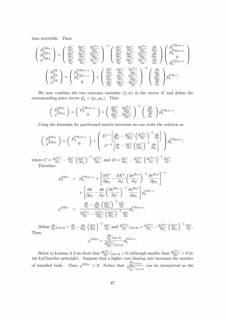
thus invertible. Then

0@

pSBcs¸

pSBcsw

'SBcs

1A =

0B@

@¸¤@p¸

@we¤@p¸

@cHe¤@p¸

@¸¤@pw

@we¤@pw

@cHe¤@pw

@¸¤@'

@we¤@'

@cHe¤@'

1CA

¡10B@

@¸¤@p¸

@we¤@p¸

@cHe¤@p¸

@k@p¸

@¸¤@pw

@we¤@pw

@cHe¤@pw

@k@pw

@¸¤@'

@we¤@'

@cHe¤@'

@k@'

1CA

0BB@

pFBcs++¸

pFBcs++w

0

pFBcs++k

1CCA

0@

pSB¸pSBw'SB

1A =

0@

pFBcs++¸

pFBcs++w

0

1A+

0B@

@¸¤@p¸

@we¤@p¸

@cHe¤@p¸

@¸¤@pw

@we¤@pw

@cHe¤@pw

@¸¤@'

@we¤@'

@cHe¤@'

1CA

¡10B@

@k@p¸@k@pw@k@'

1CApFB++

k :

We now combine the two outcome variables (¸;w) in the vector ¤0 and de…ne thecorresponding price vector p0¤ = (p¸; pw). Then

µpSBcs¤

'SBcs

¶=

µpFBcs++¤

0

¶+

Ã@¤¤0@p¤

@cHe¤@p¤

@¤¤0@'

@cHe¤@'

!¡1Ã @k@p¤@k@'

!pFBcs++k :

Using the formulae for partitioned matrix inversion we can write the solution as

µpSBcs¤

'SBcs

¶=

µpFBcs++¤

0

¶+

0BB@

D¡1

·@k@p¤

¡ @cHe¤@p¤

³@cHe¤@'

´¡1@k@'

¸

C¡1

·@k@' ¡ @¤¤0

@'

³@¤¤0@p¤

´¡1@k@p¤

¸

1CCA pFBcs++

k ;

where C = @cHe¤@' ¡ @¤¤0

@'

³@¤¤0@p¤

´¡1@cHe¤@p¤

and D = @¤¤0@p¤

¡ @cHe¤@p¤

³@cHe¤@'

´¡1@¤¤0@' .

Therefore

pSBcs¤ = pFBcs++

¤ +

"@¤¤0

@p¤¡ @¤¤0

@'

µ@cHe¤

@'

¶¡1@cHe¤

@p¤

#¡1

£"@k

@p¤¡ @k

@'

µ@cHe¤

@'

¶¡1@cHe¤

@p¤

#pFB++k

'SBcs =

@k@' ¡ @k

@p0¤

³@¤¤0@p¤

´¡1@¤¤@'

@cHe¤@' ¡ @cHe¤

@p0¤

³@¤¤0@p¤

´¡1@¤¤@'

pFBcs++k :

De…ne @k@' jd¤=0 = @k

@'¡ @k@p0¤

³@¤¤@p¤

´¡1@¤¤@' and @cHe¤

@' jd¤=0 = @cHe¤@' ¡ @cHe¤

@p0¤

³@¤¤0@p¤

´¡1@¤¤@' .

Then

'SBcs =@k@' jd¤=0

@cHe¤@' jd¤=0

pFB++k :

Below in Lemma A.3 we show that @cHe¤@' jd¤=0 > 0 (although smaller than @cHe¤

@' > 0 bythe LeChatelier principle). Suppose that a higher cost sharing rate increases the number

of installed beds. Then 'SBcs > 0. Notice that@k@'

jd¤=0

@cHe¤@'

jd¤=0

can be interpreted as the

47

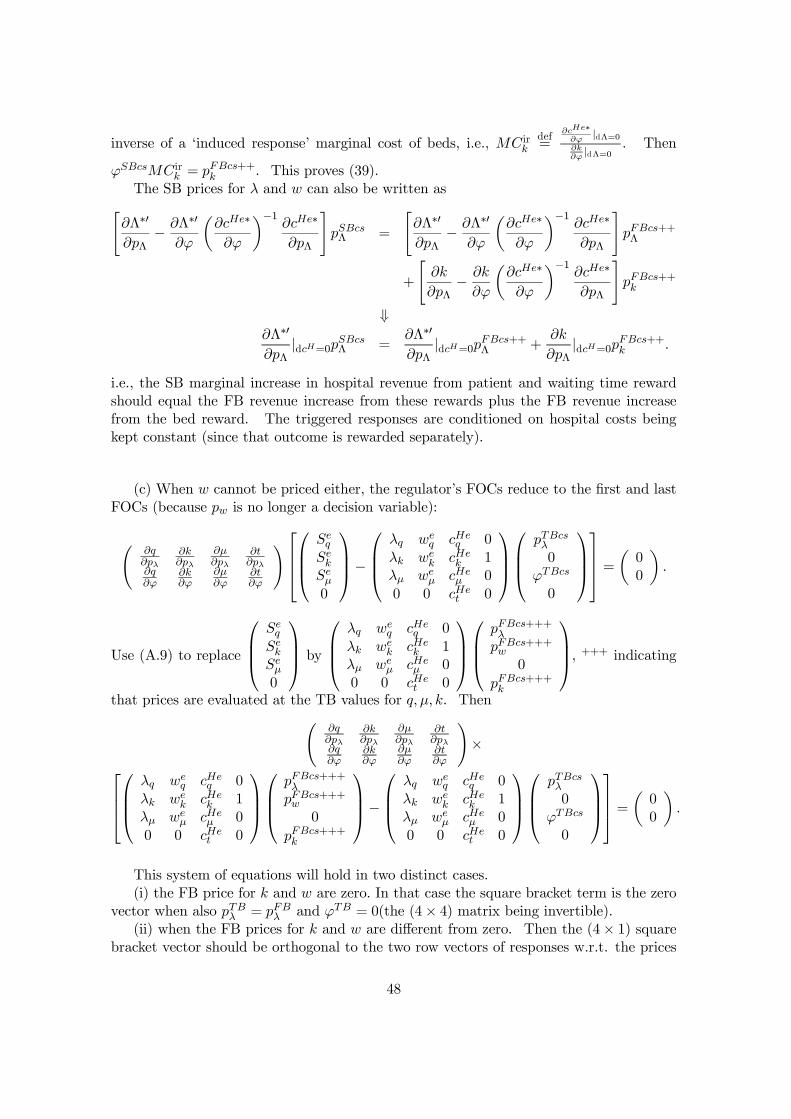
inverse of a ‘induced response’ marginal cost of beds, i.e., MC irk

def=

@cHe¤@'

jd¤=0

@k@'

jd¤=0. Then

'SBcsMCirk = pFBcs++

k . This proves (39).The SB prices for ¸ and w can also be written as

"@¤¤0

@p¤¡ @¤¤0

@'

µ@cHe¤

@'

¶¡1@cHe¤

@p¤

#pSBcs¤ =

"@¤¤0

@p¤¡ @¤¤0

@'

µ@cHe¤

@'

¶¡1@cHe¤

@p¤

#pFBcs++¤

+

"@k

@p¤¡ @k

@'

µ@cHe¤

@'

¶¡1@cHe¤

@p¤

#pFBcs++k

+@¤¤0

@p¤jdcH=0p

SBcs¤ =

@¤¤0

@p¤jdcH=0p

FBcs++¤ +

@k

@p¤jdcH=0p

FBcs++k :

i.e., the SB marginal increase in hospital revenue from patient and waiting time rewardshould equal the FB revenue increase from these rewards plus the FB revenue increasefrom the bed reward. The triggered responses are conditioned on hospital costs beingkept constant (since that outcome is rewarded separately).

(c) When w cannot be priced either, the regulator’s FOCs reduce to the …rst and lastFOCs (because pw is no longer a decision variable):

Ã@q@p¸

@k@p¸

@¹@p¸

@t@p¸

@q@'

@k@'

@¹@'

@t@'

!2664

0BB@

Seq

Sek

Se¹

0

1CCA¡

0BB@

¸q weq cHe

q 0¸k we

k cHek 1

¸¹ we¹ cHe

¹ 0

0 0 cHet 0

1CCA

0BB@

pTBcs¸

0'TBcs

0

1CCA

3775 =

µ00

¶:

Use (A.9) to replace

0BB@

Seq

Sek

Se¹

0

1CCA by

0BB@

¸q weq cHe

q 0

¸k wek cHe

k 1¸¹ we

¹ cHe¹ 0

0 0 cHet 0

1CCA

0BB@

pFBcs+++¸

pFBcs+++w

0

pFBcs+++k

1CCA, +++ indicating

that prices are evaluated at the TB values for q; ¹; k. ThenÃ

@q@p¸

@k@p¸

@¹@p¸

@t@p¸

@q@'

@k@'

@¹@'

@t@'

!£

2664

0BB@

¸q weq cHe

q 0¸k we

k cHek 1

¸¹ we¹ cHe

¹ 00 0 cHe

t 0

1CCA

0BB@

pFBcs+++¸pFBcs+++w

0

pFBcs+++k

1CCA¡

0BB@

¸q weq cHe

q 0¸k we

k cHek 1

¸¹ we¹ cHe

¹ 00 0 cHe

t 0

1CCA

0BB@

pTBcs¸

0'TBcs

0

1CCA

3775 =

µ00

¶:

This system of equations will hold in two distinct cases.(i) the FB price for k and w are zero. In that case the square bracket term is the zero

vector when also pTB¸ = pFB¸ and 'TB = 0(the (4£ 4) matrix being invertible).

(ii) when the FB prices for k and w are di¤erent from zero. Then the (4£ 1) squarebracket vector should be orthogonal to the two row vectors of responses w.r.t. the prices

48

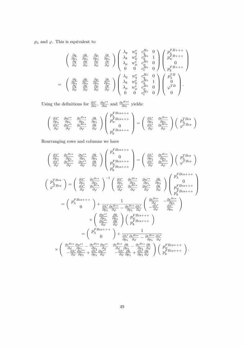
p¸ and '. This is equivalent to

Ã@q@p¸

@k@p¸

@¹@p¸

@t@p¸

@q@'

@k@'

@¹@'

@t@'

!0BB@

¸q weq cHe

q 0¸k we

k cHek 1

¸¹ we¹ cHe

¹ 00 0 cHe

t 0

1CCA

0BB@

pFB+++¸pFB+++w

0

pFB+++k

1CCA

=

Ã@q@p¸

@k@p¸

@¹@p¸

@t@p¸

@q@'

@k@'

@¹@'

@t@'

!0BB@

¸q weq cHe

q 0¸k we

k cHek 1

¸¹ we¹ cHe

¹ 00 0 cHe

t 0

1CCA

0BB@

pTB¸0

'TB

0

1CCA :

Using the de…nitions for @¸¤@m , @we¤

@m and @cHe¤@m yields:

Ã@¸¤@p¸

@we¤@p¸

@cHe¤@p¸

@k@p¸

@¸¤@'

@we¤@'

@cHe¤@'

@k@'

!0BB@

pFBcs+++¸

pFBcs+++w

0

pFBcs+++k

1CCA =

Ã@¸¤@p¸

@cHe¤@p¸

@¸¤@'

@cHe¤@'

!µpTBcs¸

'TBcs

¶

Rearranging rows and columns we have

Ã@¸¤@p¸

@cHe¤@p¸

@we¤@p¸

@k@p¸

@¸¤@'

@cHe¤@'

@we¤@'

@k@'

!0BB@

pFBcs+++¸

0pFBcs+++w

pFBcs+++k

1CCA =

Ã@¸¤@p¸

@cHe¤@p¸

@¸¤@'

@cHe¤@'

!µpTBcs¸

'TBcs

¶

µpTBcs¸

'TBcs

¶=

Ã@¸¤@p¸

@cHe¤@p¸

@¸¤@'

@cHe¤@'

!¡1à @¸¤@p¸

@cHe¤@p¸

@we¤@p¸

@k@p¸

@¸¤@'

@cHe¤@'

@we¤@'

@k@'

!0BB@

pFBcs+++¸

0pFBcs+++w

pFBcs+++k

1CCA

=

µpFBcs+++¸

0

¶+

1@¸¤@p¸

@cHe¤@' ¡ @cHe¤

@p¸@¸¤@'

Ã@cHe¤@' ¡@cHe¤

@p¸

¡@¸¤@'

@¸¤@p¸

!

£Ã

@we¤@p¸

@k@p¸

@we¤@'

@k@'

!µpFBcs+++w

pFBcs+++k

¶

=

µpFBcs+++¸

0

¶+

1@¸¤@p¸

@cHe¤@' ¡ @cHe¤

@p¸@¸¤@'

£Ã

@cHe¤@'

@we¤@p¸

¡ @cHe¤@p¸

@we¤@'

@cHe¤@'

@k@p¸

¡ @cHe¤@p¸

@k@'

¡@¸¤@'

@we¤@p¸

+ @¸¤@p¸

@we¤@' ¡@¸¤

@'@k@p¸

+ @¸¤@p¸

@k@'

!µpFBcs+++w

pFBcs+++k

¶:

49

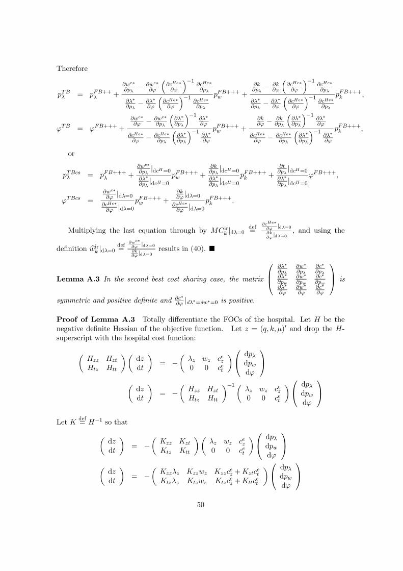
Therefore

pTB¸ = pFB++¸ +

@we¤@p¸

¡ @we¤@'

³@cHe¤@'

´¡1@cHe¤@p¸

@¸¤@p¸

¡ @¸¤@'

³@cHe¤@'

´¡1@cHe¤@p¸

pFB+++w +

@k@p¸

¡ @k@'

³@cHe¤@'

´¡1@cHe¤@p¸

@¸¤@p¸

¡ @¸¤@'

³@cHe¤@'

´¡1@cHe¤@p¸

pFB+++k ;

'TB = 'FB+++ +

@we¤@' ¡ @we¤

@p¸

³@¸¤@p¸

´¡1@¸¤@'

@cHe¤@' ¡ @cHe¤

@p¸

³@¸¤@p¸

´¡1@¸¤@'

pFB+++w +

@k@' ¡ @k

@p¸

³@¸¤@p¸

´¡1@¸¤@'

@cHe¤@' ¡ @cHe¤

@p¸

³@¸¤@p¸

´¡1@¸¤@'

pFB+++k ;

or

pTBcs¸ = pFB+++

¸ +@we¤@p¸

jdcH=0

@¸¤@p¸

jdcH=0

pFB+++w +

@k@p¸

jdcH=0

@¸¤@p¸

jdcH=0

pFB+++k +

@t@p¸

jdcH=0

@¸¤@p¸

jdcH=0

'FB+++;

'TBcs =@we¤@' jd¸=0

@cHe¤@' jd¸=0

pFB+++w +

@k@' jd¸=0

@cHe¤@' jd¸=0

pFB+++k :

Multiplying the last equation through by MC irk jd¸=0

def=

@cHe¤@'

jd¸=0

@k@'

jd¸=0, and using the

de…nition bwirk jd¸=0

def=

@we¤@'

jd¸=0

@k@'

jd¸=0results in (40). ¥

Lemma A.3 In the second best cost sharing case, the matrix

0B@

@¸¤@p¸

@w¤@p¸

@c¤@p¸

@¸¤@pw

@w¤@pw

@c¤@pw

@¸¤@'

@w¤@'

@c¤@'

1CA is

symmetric and positive de…nite and @c¤@' jd¸¤=dw¤=0 is positive.

Proof of Lemma A.3 Totally di¤erentiate the FOCs of the hospital. Let H be thenegative de…nite Hessian of the objective function. Let z = (q; k; ¹)0 and drop the H-superscript with the hospital cost function:

µHzz Hzt

Htz Htt

¶µdzdt

¶= ¡

µ¸z wz cez0 0 cet

¶0@

dp¸dpwd'

1A

µdzdt

¶= ¡

µHzz Hzt

Htz Htt

¶¡1µ¸z wz cez0 0 cet

¶0@

dp¸dpwd'

1A

Let K def= H¡1 so that

µdzdt

¶= ¡

µKzz Kzt

Ktz Ktt

¶µ¸z wz cez0 0 cet

¶0@

dp¸dpwd'

1A

µdzdt

¶= ¡

µKzz¸z Kzzwz Kzzc

ez +Kztc

et

Ktz¸z Ktzwz Ktzcez +Kttc

et

¶0@

dp¸dpwd'

1A

50

De…ne ¤ =¡¸w

¢and ¤z =

¡¸0zw0z

¢where ¸z = (¸q; ¸k; ¸¹)

0 and wz = (wq; wk; w¹)0. Also

de…ne ce0z = (ceq; cek; c

e¹) Then d¤ = ¤zdz, and dc = ce0z dz + cetdt, and we can write

µd¤dc

¶= ¡

µ¤z 0ce0z cet

¶µKzz Kzt

Ktz Ktt

¶µ¤0z cez

00 cet

¶µdp¤d'

¶

= ¡µ

¤zKzz¤0z ¤z (Kzzc

ez +Kztc

et )

(ce0z Kzz + cetKtz)¤0z ce0z Kzzc

ez + 2cetKtzc

ez + cetKttc

et

¶µdp¤d'

¶

Since the K matrix is negative de…nite by the second order condition, the matrix¡ d¤

dp0¤

d¤d'

dcdp0

¤

dcd'

¢is symmetric and positive de…nite, implying that d¸¤

dpw= dw¤

dp¸, d¸¤

d' = dc¤dp¸

, dw¤d' =

dc¤dpw

and d¸¤dp¸

> 0; dw¤

dpw> 0 and dc¤

d' > 0.

Now suppose that the vector ¤ cannot change: d¤ = 0. Then the prices for outputand waiting time need to adjust to keep ¸ and w constant:

dp¤ = ¡¡¤zKzz¤

0z

¢¡1¤z (Kzzc

ez +Kztc

et )d'

Therefore, the induced response change in hospital cost following d' when output andwaiting time are held …xed is given by

dce

d'jd¤=0 =

¡ce0z Kzz + cetKtz

¢¤0z

¡¤zKzz¤

0z

¢¡1¤z (Kzzc

ez +Kztc

et )

¡£ce0z Kzzc

ez + 2cetKtzc

ez + cetKttc

et

¤

which is positive but smaller than dced' (LeChatelier principle). ¥

51