AUTHOR

Eren Çam

EWI Working Paper, No 20/05

November 2020

Institute of Energy Economics at the University of Cologne (EWI)

www.ewi.uni-koeln.de

Optimal Dispatch of a Coal-Fired Power Plant with

Integrated Thermal Energy Storage

CORRESPONDING AUTHOR

Eren Çam

Institute of Energy Economics at the University of Cologne (EWI)

eren.cam@ewi.uni-koeln.de

ISSN: 1862-3808

The responsibility for working papers lies solely with the authors. Any views expressed are

those of the authors and do not necessarily represent those of the EWI.

Institute of Energy Economics

at the University of Cologne (EWI)

Alte Wagenfabrik

Vogelsanger Str. 321a

50827 Köln

Germany

Tel.: +49 (0)221 277 29-100

Fax: +49 (0)221 277 29-400

www.ewi.uni-koeln.de

Optimal Dispatch of a Coal-Fired Power Plant with Integrated ThermalEnergy Storage

Eren Cam

Abstract

As the share of intermittent renewable electricity generation increases, the remaining fleet of conventional

power plants will have to operate with higher flexibility. One of the methods to increase power plant

flexibility is to integrate a thermal energy storage (TES) into the water-steam cycle of the plant. TES can

provide flexibility and achieve profits by engaging in energy arbitrage on the spot markets and by providing

additional power on the control power markets. This paper considers a reference coal-fired power plant with

an integrated TES system for the year 2019 in Germany. Optimal dispatch for profit maximisation with

TES is simulated on the hourly day-ahead and quarter-hourly continuous intraday markets as well as on the

markets for primary (PRL) and secondary (SRL) control power. Analysing the effects of TES round-trip

efficiency and storage capacity on dispatch and the profits, I find that smaller TES systems with up to

one hour of storage capacity can achieve substantial profits on the PRL market while also realising profits

from energy arbitrage on the continuous intraday market. Higher TES round-trip efficiencies can help TES

achieve significant profits also on the day-ahead market. The analysis shows that a storage capacity of 2–3

hours is enough to realise most of the energy arbitrage potential, while larger storage capacities can greatly

increase TES profits on the SRL market. Small TES systems are found to increase the full load hours of

the plant marginally. However, the increase becomes significant with larger storage capacities and can lead

to higher CO2 emissions for the individual plant.

Keywords: coal-fired power plant, flexibility, thermal energy storage, energy arbitrage

JEL classification: Q40, Q49

1

1. Introduction

The share of renewable energies in global electricity generation has grown substantially in the last decades

and is expected to further increase in the future. International Energy Agency, in its Stated Policies scenario

of the World Energy Outlook 2019, foresees the global share of wind and solar PV in the electricity mix

to increase from 7% in 2018 to 17.2% in 2030. In the Sustainable Development scenario, which considers a

setting with a higher probability of reaching the climate targets, this share increases to 25% (IEA, 2019).

Intermittent renewable generation is highly weather-dependent and fluctuations are largely compensated by

conventional power plants in the current energy system. As the share of intermittent renewables further

increases and conventional capacity decreases, the remaining fleet of conventional power plants will need to

operate with increased flexibility.1

The main specifications of a conventional power plant that define its flexibility are its minimum load,

load change rate (i.e. ramping rate), and start-up duration and start-up costs.2 A relatively flexible plant

would be characterised by a low minimum load, a high load change rate and low start-up duration with

lower start-up costs. While lowering the minimum load of the plant reduces the losses in low price hours and

helps avoid shut-downs and subsequent start-ups, increasing the load change rate would allow to generate

additional revenues on the electricity markets (e.g. on intraday and control power markets). As such,

increased flexibility can directly translate to higher profits for the power plant operator. Additionally,

increased flexibility of power plants can also have system benefits as they allow the integration of more wind

and solar power (Agora Energiewende, 2017). With increased wind penetration, the ramping capabilities of

the existing power plant fleet becomes much more important, since more flexible operation of the existing

fleet would allow for a higher degree of intermittent wind integration (Hong et al., 2012). Moreover, flexible

thermal power plants can help reduce wind curtailment and increase resilience to wind ramping (Kubik

et al., 2015).

An effective method to increase power plant flexibility is to utilise thermal energy storages (TES). Zhao

et al. (2018b) and Zhao et al. (2018a) simulate a coal-fired power plant and show that, by controlling the

internal thermal storages inherent to the thermal system of the plant, it is possible to enhance the ramping

rate of the plant.3 More substantial increases in flexibility are possible by integrating a thermal energy

1Using optimal power flow simulations to compare the years 2013 and 2020, Eser et al. (2016) finds that increased penetrationof renewables in Central Western and Eastern Europe can cause the number of starts of power plants to increase by up to 23%and the number of load ramps by up to 181%.

2For more information on these parameters, see Hentschel et al. (2016), Agora Energiewende (2017) and Richter et al.(2019).

3Among the strategies investigated in these papers, the largest additional contribution to ramping rates has an averagepower ramp rate of 6.19% per minute (40.89 MW/min) with a very limited energy capacity of 5.58 MWh.

2

storage into the water-steam cycle of the plant. With these configurations, the TES is charged with the heat

extracted from the water-steam cycle of the plant when power demand is low (i.e. electricity prices are low)

and the stored energy is then discharged to the plant cycle when power demand is high (i.e. electricity prices

are high), allowing energy arbitrage to be conducted. Wojcik and Wang (2017) investigate the integration

of a TES into a sub-critical oil-fired conventional power plant, focusing on the simulation of charging and

discharging processes. Li et al. (2017) consider a combined-cycle gas turbine plant with integrated TES. Li

and Wang (2018) and Cao et al. (2020) analyse the feasibility of integrating a high temperature thermal

energy storage in a coal-fired power plant. Richter et al. (2019), also simulating a coal-fired plant, consider

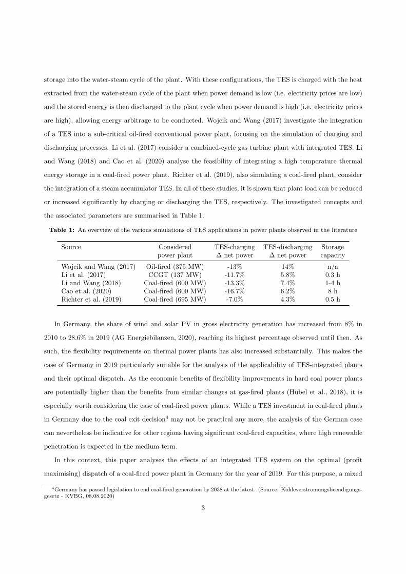
the integration of a steam accumulator TES. In all of these studies, it is shown that plant load can be reduced

or increased significantly by charging or discharging the TES, respectively. The investigated concepts and

the associated parameters are summarised in Table 1.

Table 1: An overview of the various simulations of TES applications in power plants observed in the literature

Source Considered TES-charging TES-discharging Storagepower plant ∆ net power ∆ net power capacity

Wojcik and Wang (2017) Oil-fired (375 MW) -13% 14% n/aLi et al. (2017) CCGT (137 MW) -11.7% 5.8% 0.3 hLi and Wang (2018) Coal-fired (600 MW) -13.3% 7.4% 1-4 hCao et al. (2020) Coal-fired (600 MW) -16.7% 6.2% 8 hRichter et al. (2019) Coal-fired (695 MW) -7.0% 4.3% 0.5 h

In Germany, the share of wind and solar PV in gross electricity generation has increased from 8% in

2010 to 28.6% in 2019 (AG Energiebilanzen, 2020), reaching its highest percentage observed until then. As

such, the flexibility requirements on thermal power plants has also increased substantially. This makes the

case of Germany in 2019 particularly suitable for the analysis of the applicability of TES-integrated plants

and their optimal dispatch. As the economic benefits of flexibility improvements in hard coal power plants

are potentially higher than the benefits from similar changes at gas-fired plants (Hubel et al., 2018), it is

especially worth considering the case of coal-fired power plants. While a TES investment in coal-fired plants

in Germany due to the coal exit decision4 may not be practical any more, the analysis of the German case

can nevertheless be indicative for other regions having significant coal-fired capacities, where high renewable

penetration is expected in the medium-term.

In this context, this paper analyses the effects of an integrated TES system on the optimal (profit

maximising) dispatch of a coal-fired power plant in Germany for the year of 2019. For this purpose, a mixed

4Germany has passed legislation to end coal-fired generation by 2038 at the latest. (Source: Kohleverstromungsbeendigungs-gesetz - KVBG, 08.08.2020)

3

integer linear programming (MILP) model is developed to simulate the optimal dispatch of the plant with

TES. Additional profits due to TES on various electricity markets (i.e. day-ahead, intraday, primary (PRL)

and secondary (SRL) control power markets)5 are calculated. The relevance of individual TES parameters

regarding the profit potential on the individual markets is analysed and charging/discharging patterns are

identified.

Considering a reference TES system specification as presented in Richter et al. (2019), I find that the

TES with a 0.5 hours of storage capacity can achieve 377,000 EUR of additional profits in the dispatch year

of 2019, increasing the total profits of the plant by 2.4%. Profits on the PRL market are found to make up

a large majority (about 60%) of the profits, followed by those obtained via energy arbitrage due to dispatch

on the intraday continuous market (about 20%). Larger storage capacities allow for higher energy arbitrage

profits; albeit the incrase in profits due to arbitrage is limited. In contrast, very substantial increases in the

profits on the SRL market can be achieved with larger storage capacities. Considering also an alternative

high-efficiency TES, I show that energy arbitrage profits on both day-ahead and intraday markets can be

greatly increased if the round-trip efficiency of the TES system is higher. While the analysis shows that

integrating a TES system can provide the plant with significant additional flexibility and profits, TES is

found to increase the full load hours of the plant. The increase is marginal (less than 1%) for a TES storage

capacity of 0.5 h; however, it becomes significant with larger capacities and can potentially increase the CO2

emissions of the individual plant.

This paper is primarily related to two streams of literature. The first relevant stream of literature deals

with simulating optimal dispatch using MILP models. MILP models have been widely used in the literature

for solving unit commitment problems (see Ostrowski et al. (2012), Frangioni et al. (2009) and Richter

et al. (2016)). It is also common to apply MILP models to determine optimal scheduling of individual

power plants and to simulate profitability and conduct techno-economic analyses. Kazempour et al. (2008)

provides an optimal dispatch model for a pumped-storage plant that is active in both energy and regulation

markets, simulating expected weekly profits. Knaut and Paschmann (2017) uses a MILP model to compare

profitability of a CCGT plant to that of a lignite-fired power plant on different electricity markets in Germany

(i.e. day-ahead auction and intraday auction). Beiron et al. (2020) analyses various flexibility options using a

MILP optimal dispatch model for a waste incineration plant with combined heat and power (CHP). Similarly,

Beiron et al. (2020) uses a MILP-based approach for the analysis of a CCGT CHP plant’s flexibility potential.

5PRL is also referred to as Frequency Containment Reserve (FCR.) SRL is also referred to as Frequency Restoration Reservewith Automatic Activation (aFRR)

4

The second stream of literature relevant to this paper focuses on techno-economic assessment of storage

systems and energy arbitrage. Energy arbitrage with storage systems has been a common topic in

literature (see Walawalkar et al. (2007), Sioshansi et al. (2009) and Bradbury et al. (2014)), where the

research has focused on optimal location, sizing and parametrisation of various storage technologies. With

decreasing battery costs, recent years have especially seen a surge in studies analysing energy arbitrage

with Li-Ion batteries. Dufo-Lopez (2015), simulating the operation of a Li-Ion battery storage system for

the Spanish electricity market pool of 2013, finds that the considered storage system is not profitable with

the contemporary investment costs. Arcos-Vargas et al. (2020), similarly considering a Li-Ion battery

system for the Iberian market during the period 2016–2017, finds that energy arbitrage will only be

profitable from 2024 onward with sustained decreases in battery costs. Metz and Saraiva (2018) simulates

energy arbitrage with a Li-Ion battery on the German hourly and quarter-hourly intraday auctions for the

period 2011–2016, finding that the analysed system does not break even with the historical volatility of

prices and the contemporary storage investment costs.

Energy arbitrage with TES has been considered in the literature for different types of energy systems.

Sioshansi and Denholm (2010) shows that TES can increase the value of concentrated solar power (CSP)

plants as it allows the shifting of generation to hours with higher electricity prices. Scapino et al. (2020)

considers an energy system with sorption TES for the electricity markets of Belgium in 2013 and the UK

in 2017, and finds that the TES system is not profitable when only operating on the day-ahead market,

but becomes profitable when it also provides balancing services. Risthaus and Madlener (2017) simulates

the optimal dispatch of a heat pump with TES, which is integrated partially6 (i.e. only for the discharging

phase) to a coal-fired power plant and a CCGT in Germany, as well as to a CSP in Spain, for the year of

2016. The study finds that revenues from energy arbitrage are not enough to cover the high investment

costs.

Against this backdrop, the contribution of this paper can be summarised as follows: The analysis

conducted in this paper is the first of its kind, providing insight into the optimal dispatch of a coal-fired

plant with a TES that is completely integrated in the steam-water cycle. Moreover, the paper

distinguishes itself by the inclusion of the primary and secondary control power markets as well as the

intraday continuous market in the dispatch simulation. Optimal profits of the system in the participated

spot and control powers are calculated and the effects of TES parametrisation on dispatch and profits are

6During the charging phase, the heat is generated by the heat pump and is stored in the TES. The heat is then suppliedfrom the TES to the plant water-steam cycle during discharging.

5

investigated. The analysis is conducted for a power plant located in Germany with German historical

market prices. However, the methodology can also be applied to other regions.

2. Model

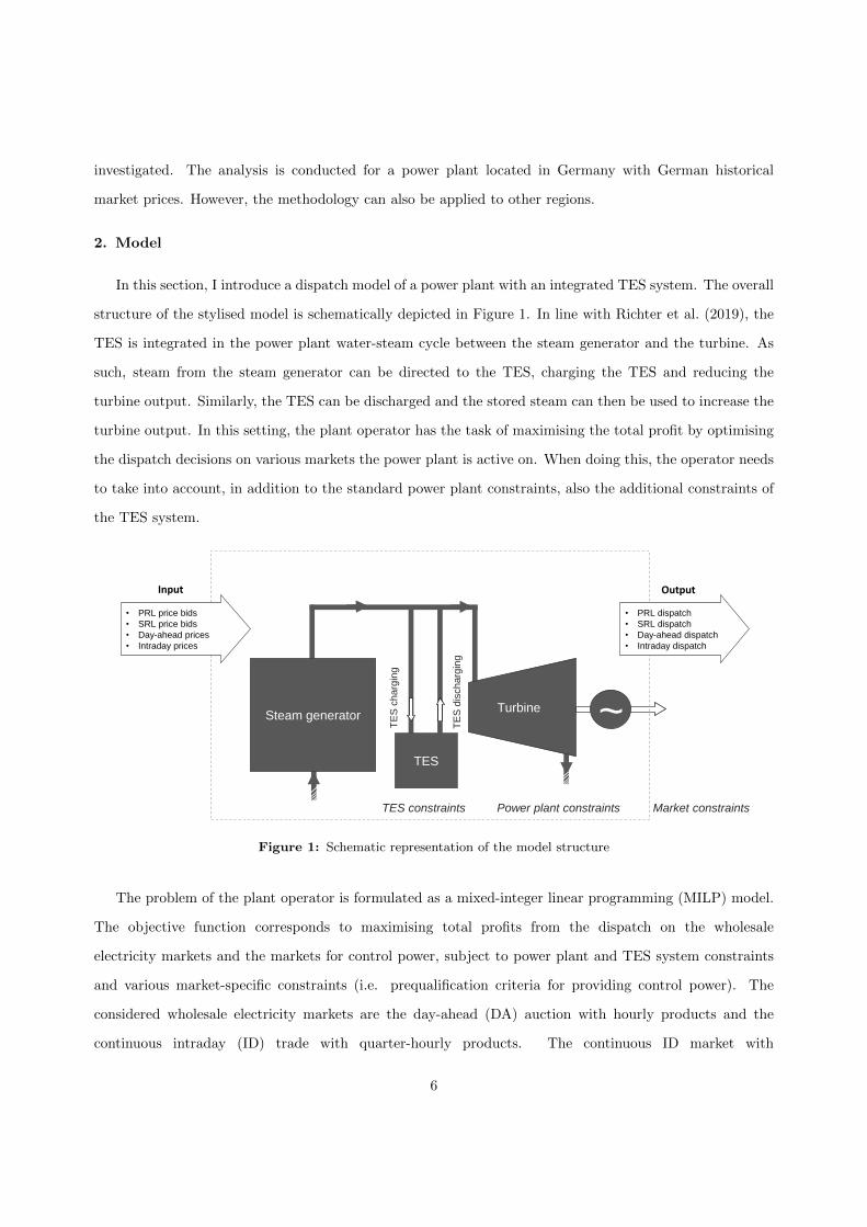
In this section, I introduce a dispatch model of a power plant with an integrated TES system. The overall

structure of the stylised model is schematically depicted in Figure 1. In line with Richter et al. (2019), the

TES is integrated in the power plant water-steam cycle between the steam generator and the turbine. As

such, steam from the steam generator can be directed to the TES, charging the TES and reducing the

turbine output. Similarly, the TES can be discharged and the stored steam can then be used to increase the

turbine output. In this setting, the plant operator has the task of maximising the total profit by optimising

the dispatch decisions on various markets the power plant is active on. When doing this, the operator needs

to take into account, in addition to the standard power plant constraints, also the additional constraints of

the TES system.

Steam generator ~Turbine

TE

Sdis

charg

ing

TE

Scharg

ing

TES

TES constraints Power plant constraints Market constraints

• PRL price bids

• SRL price bids

• Day-ahead prices

• Intraday prices

• PRL dispatch

• SRL dispatch

• Day-ahead dispatch

• Intraday dispatch

Input Output

Figure 1: Schematic representation of the model structure

The problem of the plant operator is formulated as a mixed-integer linear programming (MILP) model.

The objective function corresponds to maximising total profits from the dispatch on the wholesale

electricity markets and the markets for control power, subject to power plant and TES system constraints

and various market-specific constraints (i.e. prequalification criteria for providing control power). The

considered wholesale electricity markets are the day-ahead (DA) auction with hourly products and the

continuous intraday (ID) trade with quarter-hourly products. The continuous ID market with

6

quarter-hourly products is particularly chosen due to its higher volatility, which makes it theoretically

more profitable for storage systems. Additionally, the plant is assumed to provide primary and secondary

control power, PRL and SRL, respectively.

Taking prices for the PRL, SRL, DA and ID markets as input, the model optimises the dispatch on

these markets. Optimising the dispatch on PRL and SRL markets simultaneously with the DA market

allows the optimal capacities on the control power markets to be endogenously determined by the model.

The coal-fired plant without the TES system is assumed not to be able to participate on the continuous ID

market by itself as it lacks the necessary operational flexibility. The TES, however, can be activated within

several minutes (Richter et al., 2019), providing the necessary flexibility to be able to react to price signals

and offer capacities on the continuous ID market. Similarly, the TES increases the technical capability for

providing control power on the PRL and SRL markets. The plant operator is assumed to be price taker

and to have perfect foresight. Therefore, the optimal total profit obtained by the model represents an upper

benchmark.

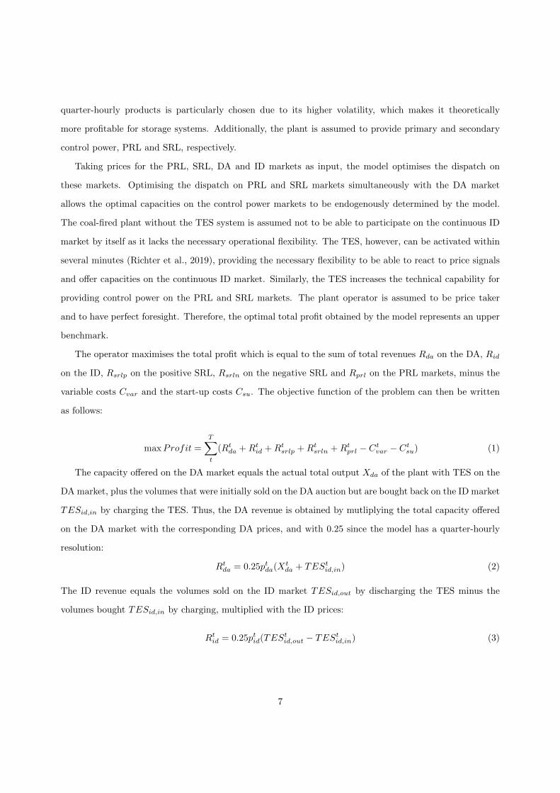
The operator maximises the total profit which is equal to the sum of total revenues Rda on the DA, Rid

on the ID, Rsrlp on the positive SRL, Rsrln on the negative SRL and Rprl on the PRL markets, minus the

variable costs Cvar and the start-up costs Csu. The objective function of the problem can then be written

as follows:

maxProfit =

T∑t

(Rtda +Rt

id +Rtsrlp +Rt

srln +Rtprl − Ct

var − Ctsu) (1)

The capacity offered on the DA market equals the actual total output Xda of the plant with TES on the

DA market, plus the volumes that were initially sold on the DA auction but are bought back on the ID market

TESid,in by charging the TES. Thus, the DA revenue is obtained by mutliplying the total capacity offered

on the DA market with the corresponding DA prices, and with 0.25 since the model has a quarter-hourly

resolution:

Rtda = 0.25ptda(Xt

da + TEStid,in) (2)

The ID revenue equals the volumes sold on the ID market TESid,out by discharging the TES minus the

volumes bought TESid,in by charging, multiplied with the ID prices:

Rtid = 0.25ptid(TESt

id,out − TEStid,in) (3)

7

On top of the standalone SRL capability PLsrlp of the plant, TES can provide additional positive

SRL capacity TESsrlp by discharging. The revenue obtained on the positive SRL market consists of two

components: the capacity component and the energy component. The operator generates revenue by offering

control power capacity, independent of whether the plant is activated for SRL or not. The price it receives

per MW of capacity is represented by psrlp,c. As for the energy component, I assume that the plant can be

activated for positive SRL with an exogenous average probability of wsrlp, receiving the SRL energy price

of psrlp,e. Similarly, TES can increase the total negative SRL offered by the plant by TESsrln on top of the

standalone capacity PLsrln. The operator receives the capacity price psrln,c, and with an average probability

of wsrln the energy price psrln,e. The capacity prices for both positive and negative SRL products (psrlp,c

and psrln,c) correspond to the pay-as-bid capacity prices of the power plant, which are directly derived from

its opportunity costs over the DA market7 and are limited by the historical marginal capacity prices. The

revenues for providing positive and negative SRL then become:

Rtsrlp = (ptsrlp,c + 0.25ptsrlp,ewsrlp)(PLt

srlp + TEStsrlp)

Rtsrln = (ptsrln,c + 0.25ptsrln,ewsrln)(PLt

srln + TEStsrln)

(4)

The standalone PRL capacity offered by the plant is PLprl. Note that PRL is a symmetrical product.

Therefore, the plant offering PRL is obligated to provide the same capacity in both directions, i.e. when it

reduces or increases output depending on the PRL activation signal. As such, being able to reduce turbine

output by charging and to increase it by discharging, TES can increase the offered PRL capacity by TESprl.

The PRL revenue is then equal to the total offered capacity multiplied by the PRL price pprl8:

Rtprl = ptprl(PL

tprl + TESt

prl) (5)

Variable costs of the plant are represented by a linear approximation of the fuel costs using the

methodology presented in Swider and Weber (2007) as shown in Equation 6. Given fuel costs pfuel and the

efficiency, the variable costs depend on the plant output Xpl, the upper bound of which is defined by the

maximum plant capacity kpl,max. The minimum load kpl,min defines its lower bound. Note that the plant

output Xpl is the electrical representation of the output of the steam generator. Hence, it corresponds to

the standalone output of the plant without the TES. As the efficiency at minimum load ηml is lower than

the efficiency at full load ηfl, the operator is incentivised to reduce plant output when the wholesale prices

7See Musgens et al. (2014), Knaut et al. (2017) and Kunle (2018) for the methodology.8PRL prices are also assumed to correspond to the opportunity cost bids over the DA market, limited by the historical PRL

settlement prices.

8

are not profitable. The variable costs also include other variable costs represented by cot. Note that the

binary variable Bon is equal to 1 when the plant is online.

Ctvar = 0.25pfuel

(Xt

pl

ηfl+

(1

ηml− 1

ηfl

)(kpl,maxB

ton −Xt

pl)kpl,min

kpl,max − kpl,min

)+ 0.25cotX

tpl (6)

When the plant is switched on, it incurs start-up costs while ramping up to reach the minimum load.

Those costs mainly ensue from the usage of secondary fuel and are represented by Equation 7, where the

binary variable Bsu is equal to 1 when the plant starts up. To avoid additional complexity, the model does

not distinguish between different start-up types (e.g. cold, warm, hot); rather, a single start-up type with

average representative costs csu is assumed.

Csu = csuBtsu (7)

The plant output is defined by Equation 8, where it is either equal to zero when turned off or lies between

the minimum load and the maximum plant capacity when online.

Xtpl = kpl,minB

ton +Xt

overmin,

where Xtovermin ≤ (kpl,max − kpl,min)Bt

on

(8)

Equation 9 considers that the change in plant output between the time periods t − 1 and t (when the

plant is online in both time periods) is restricted by the load change rates; namely, equals to rup when

ramping up and rdown when ramping down. Additionally, it is ensured that when the plant has started up

and has become online, it starts at minimum load. Likewise, when the plant is shutting down, it reduces its

output to minimum load first and then to zero.

Xtpl −Xt−1

pl ≤ rupBt−1on + kpl,min(Bt

on −Bt−1on )

Xt−1pl −X

tpl ≤ rdoBt

on + kpl,min(Bt−1on −Bt

on)

(9)

The binary states of starting up Bsu and shutting down Bsd are defined, taking into account the

corresponding durations dsu and dsd, respectively:

Bton −Bt−1

on =

t1<t∑t1=t−dsu

Bt1su −

t<t1∑t=t1−dsd

Btsd (10)

An additional restriction ensures that the shut-down and start-up periods do not intersect:

Btsu +

t1≤t+dsd∑t1>t

Bt1sd +

t1≤t+dsd+dsu∑t1>t

Bt1su ≤ 1 (11)

9

At time point t, if not offline, the plant can only be active in one of the states “starting up” (Bsu),

“online” (Bon) or “shutdown” (Bsd):

Btsu +Bt

on +Btsd ≤ 1 (12)

The output level of the plant Xpl is determined by the markets it is actively providing capacity for and

whether the TES is being charged or discharged as expressed in Equation 13. Discharging the TES on the

DA market with the power TESda,out increases the total capacity active on the DA market Xda. Similarly,

charging the TES on the DA market with TESda,in decreases the total capacity active on the DA market.

The plant output level is also determined by the total positive and negative SRL provision multiplied with

the respective activation probabilities.

Xtpl + TESt

da,out − TEStda,in =Xt

da + TEStid,in

+ wsrlp(PLtsrlp + TESt

srlp)− wsrln(PLtsrln + TESt

srln)

(13)

The capacity provided in the respective markets is constrained by the physical plant restrictions. As

expressed in Equation 14, the total capacity provided on the day-ahead market (Xda + TESid,in) plus the

positive SRL and PRL capacities, in case they are fully activated, cannot be greater than the maximum

plant capacity modified by the net TES output (discharging minus charging). Similarly, Equation 15 shows

that the total day-ahead capacity minus a full activation of negative SRL and PRL capacities cannot be

lower then the minimum load of the plant, which is modified by the net TES output. Additionally, PRL

provision by the plant requires that the plant output is above a certain threshold, which necessitates the

inclusion of an additional binary term that increases the required minimum plant output by an additional

fprl percent of total plant capacity.9

Xtda + TESt

id,in + PLtsrlp + PLt

prl ≤ kpl,maxBton + TESt

da,out − TEStda,in (14)

Xtda + TESt

id,in − PLtsrln − PLt

prl ≥ kpl,minBton + fprlkpl,maxB

tprl + TESt

da,out − TEStda,in (15)

In order for the plant output with TES not to exceed the minimum and maximum achievable total load

levels when providing PRL and SRL, additional constraints are included as shown in Equations 16–18.

9The minimum PRL threshold of the plant is assumed to be 60% of full load. Hence fprl equals 40% as the minimum loadis assumed to be 20% of full load.

10

Xtda + TESt

id,in + PLtsrlp + PLt

prl + TEStid,out ≤ Bt

onkpl,max + ktes,max,out(1−Btprl) (16)

Xtda + TESt

id,in + PLtsrlp + PLt

prl + TEStid,out ≤ Bt

onkpl,max + ktes,max,out(1−Btsrl,pos) (17)

Xtda − PLt

srln ≥ Btonkpl,min − ktes,max,in(1−Bt

srl,neg) (18)

TES power output when charging and discharging depends directly on the plant output (Xpl) (Richter

et al., 2019). Therefore, I include this variation in the model by linearising the power capacity as shown in

Equation 19 with the use of exogenous parameters γ0,in and γ1,in when charging, and γ0,out and γ1,out when

discharging.

TEStda,in + TESt

id,in + TEStsrln + TESt

prl ≤ γ0,inBton + γ1,inX

tpl

TEStda,out + TESt

id,out + TEStsrlp + TESt

prl ≤ γ0,outBton + γ1,outX

tpl

(19)

TES charging and discharging power on the day-ahead and intraday markets are additionally restricted

and binary variables Btes,in (equal to 1 when charging) and Btes,out (equal to 1 when discharging) are

defined:

TEStda,in + TESt

id,in ≤ ktes,max,inBttes,in

TEStda,out + TESt

id,out ≤ ktes,max,outBttes,out

(20)

The minimum charging and discharging power for the TES are restricted at 1 MW (as the binary variables

are either 0 or 1):

TEStda,in + TESt

id,in ≥ Bttes,in

TEStda,out + TESt

id,out ≥ Bttes,out

(21)

The energy flow Etes,in into the TES is equal to the energy input by charging on the DA and ID markets

as well as charging due to activation of negative SRL, as shown in Equation 22. The overall energy losses

incurred by the TES system are considered with the average round-trip-efficiency ηtes and included in the

charging phase.10 Likewise, Equation 23 shows the energy output of the TES, Etes,out, which consists of

discharging on the DA and ID markets and the activation on the positive SRL market.

Ettes,in = 0.25ηtes(TES

tda,in + TESt

id,in + wsrlnTEStsrln) (22)

Ettes,out = 0.25(TESt

da,out + TEStid,out + wsrlpTES

tsrlp) (23)

10Note that the model and the conducted analysis in this paper assumes average round-trip efficiencies for the TES system.In reality, the round-trip efficiency varies in real-time as it also depends on the plant-load level the TES system is charged anddischarged at.

11

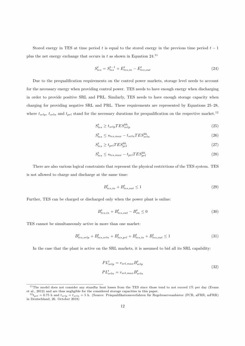
Stored energy in TES at time period t is equal to the stored energy in the previous time period t − 1

plus the net energy exchange that occurs in t as shown in Equation 24.11

Sttes = St−1

tes + Ettes,in − Et

tes,out (24)

Due to the prequalification requirements on the control power markets, storage level needs to account

for the necessary energy when providing control power. TES needs to have enough energy when discharging

in order to provide positive SRL and PRL. Similarly, TES needs to have enough storage capacity when

charging for providing negative SRL and PRL. These requirements are represented by Equations 25–28,

where tsrlp, tsrln and tprl stand for the necessary durations for prequalification on the respective market.12

Sttes ≥ tsrlpTESbh

srlp (25)

Sttes ≤ stes,max − tsrlnTESbh

srln (26)

Sttes ≥ tprlTESbh

prl (27)

Sttes ≤ stes,max − tprlTESbh

prl (28)

There are also various logical constraints that represent the physical restrictions of the TES system. TES

is not allowed to charge and discharge at the same time:

Bttes,in +Bt

tes,out ≤ 1 (29)

Further, TES can be charged or discharged only when the power plant is online:

Bttes,in +Bt

tes,out −Bton ≤ 0 (30)

TES cannot be simultaneously active in more than one market:

Bttes,srlp +Bt

tes,srln +Bttes,prl +Bt

tes,in +Bttes,out ≤ 1 (31)

In the case that the plant is active on the SRL markets, it is assumed to bid all its SRL capability:

PLtsrlp = vsrl,maxB

tsrlp

PLtsrln = vsrl,maxB

tsrln

(32)

11The model does not consider any standby heat losses from the TES since those tend to not exceed 1% per day (Evanset al., 2012) and are thus negligible for the considered storage capacities in this paper.

12tprl = 0.75 h and tsrlp = tsrln = 5 h. (Source: Praqualifikationsverfahren fur Regelreserveanbieter (FCR, aFRR, mFRR)in Deutschland, 26. October 2018)

12

The additional SRL capacity bids due to TES are allowed to vary. The maximum additional positive

and negative SRL capacities of TES are limited by the maximum discharging and charging power of the

TES, respectively.

TEStsrlp ≥ vsrl,minB

ttes,srlp

TEStsrln ≥ vsrl,minB

ttes,srln

TEStsrlp ≤ ktes,max,outB

ttes,srlp

TEStsrln ≤ ktes,max,inB

ttes,srlp

(33)

Due to technical limitations (Richter et al., 2019), TES can only provide additional capacity when the

plant is providing SRL, but cannot provide standalone SRL capacity on its own. This condition is included

with logical constraints as follows:

Btes,srlp −Bsrlp ≤ 0

Btes,srln −Bsrln ≤ 0

(34)

In the case that the plant is active on the PRL market, it is assumed to bid all its PRL capability:

PLtprl = vprl,maxB

tprl

(35)

Additional PRL capacity via TES ia allowed to vary. It cannot be less than the minimum PRL capability

vtes,prl,min of the TES and cannot be greater than the maximum PRL capability vtes,prl,max of the TES:

TEStprl ≥ vtes,prl,minB

ttes,prl

TEStprl ≤ vtes,prl,maxB

ttes,prl

(36)

Note that in contrast to SRL provision, TES can provide standalone PRL capacity even if the plant is not

providing PRL. Therefore, additional constraints such as in Equation 34 are not included for the case of

PRL provision.

Finally, the quarter hourly control power capacities are mapped to corresponding 4-hour-blocks:

PLbhsrlp = PLt

srlp, PLbhsrln = PLt

srln, PLbhprl = PLt

prl

TESbhsrlp = TESt

srlp, TESbhsrln = TESt

srln, TESbhprl = TESt

prl

(37)

The problem is solved with a quarter-hourly resolution and in weekly time blocks (i.e. T = 672).

Optimising in weekly blocks instead of a complete year helps the problem to have reduced solution times.

The weekly blocks are linked by carrying over the optimal solutions for the plant production level Xqpl and

the TES energy level Sqtes ensuing at the end of a week as the initial values to the next week.

13

3. Results

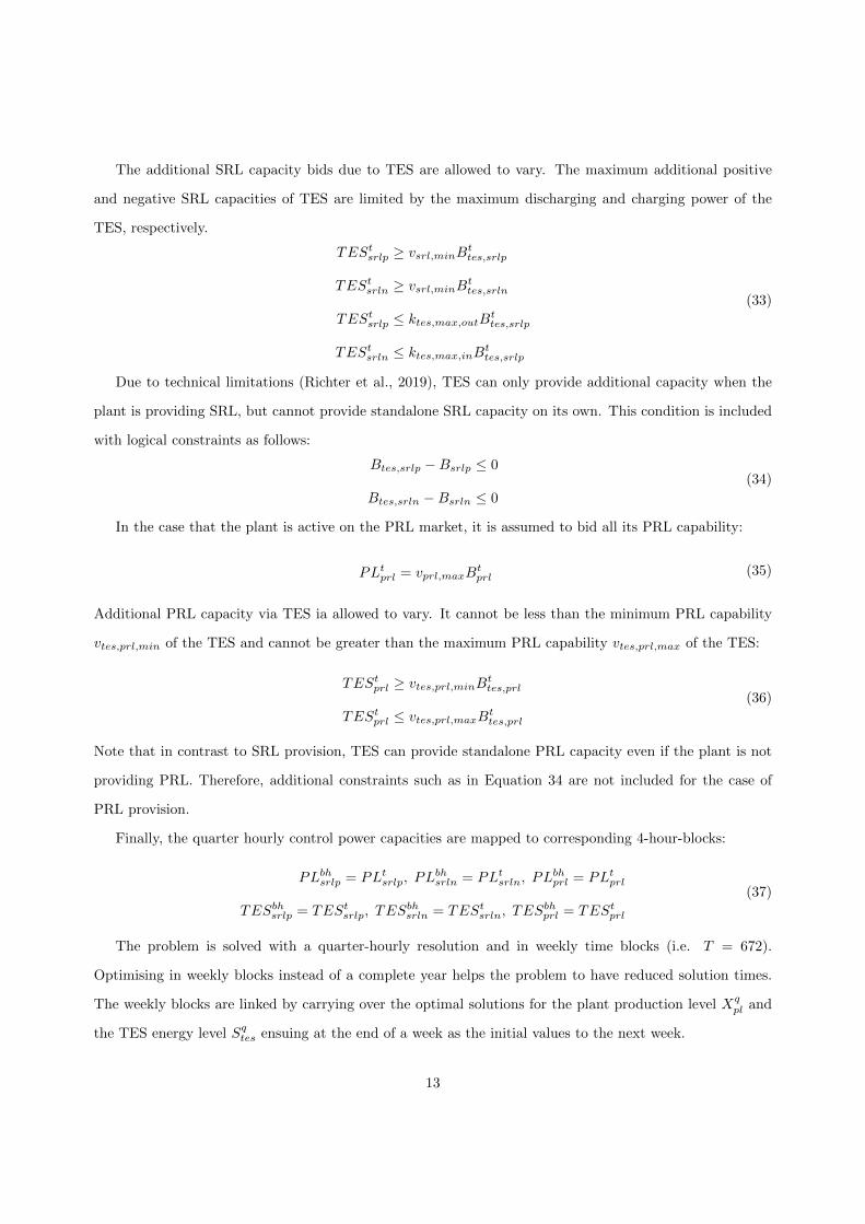
3.1. Input Data

The considered reference power plant in this paper is assumed to be a newer generation coal-fired power

plant (e.g. similar to Walsum 10 in Germany) with a relatively high efficiency and low minimum load. The

parameters of the plant are presented in Table 2.

Table 2: Input parameters assumed for the coal-fired power plant

Installed net capacity 740 MWMinimum load 148 MWEfficiency at full load 46 %Efficiency at minimum load 36.8 %Start-up duration 3 hShut-down duration 2.5 hLoad change rate ±10 MW/minuteSRL capability 50 MWPRL capability 20 MWStart-up costs 70,000 EURFuel costs 18.54 EUR/MWhth

Other variable costs 1.3 EUR/MWh

Note that start-up costs are assumed to be on average 70,000 EUR in line with Schill et al. (2016) and 1.3

EUR/MWh of other variable costs are assumed (r2b, 2019). Fuel costs include the 2019 historical average

ARA FOB thermal coal price of 9.1 EUR/MWhth plus additional transport costs of 1.25 EUR/MWhth (r2b,

2019). On top of this, costs for emission certificates are added with the average 2019 EU ETS CO2 price

of 24.86 EUR/tCO2 and an assumed specific emissions factor of 0.33 tCO2/MWhth (Agora Energiewende,

2017). The data for fuel cost calculation is presented in Table 3.

Table 3: Input data for fuel cost calculation

Thermal coal price 9.1 EUR/MWhth

Transport costs 1.25 EUR/MWhth

CO2 price 24.86 EUR/tCO2

Specific CO2 emissions 0.33 tCO2/MWhth

For input DA electricity prices, historical hourly time series data from EPEX SPOT for 2019 is used.

For the continuous ID prices, quarter hourly weighted average price series for 2019 are used. The statistics

of the input prices are summarised in Table 4. The average prices in both markets are almost identical.

However, by comparing the average daily standard deviation of the prices, it can be seen that the volatility

on the intraday market is significantly higher.

14

Table 4: Statistics of input prices on the hourly day-ahead and the quarter-hourly continuous intraday electricitymarkets (in EUR/MWh)

Mean Avg. daily std. dev. Min. Max.

Day-ahead 37.69 8.80 -90.01 121.46Intraday 37.77 12.97 -244.47 577.25

Historical marginal capacity and settlement prices for the year 2019 are used in the method of calculating

bids on SRL and PRL markets as mentioned in Section 2, respectively. For the energy prices in the SRL

market, we assume that the plant bids on average its variable costs with a mark-up. The plant is assumed

to bid double its variable costs as energy prices on the positive SRL market and half of its variable costs on

the negative SRL market. On both SRL markets, an average 20% probability of activation is assumed.

3.2. Dispatch without TES

The optimal power plant dispatch in 2019 on the German day-ahead electricity market and the control

power markets for SRL and PRL is simulated without TES. The results of the simulation are summarised in

Table 5. Market-specific profits are provided. The profits on the DA market correspond to a case where the

plant is only active on the DA market. Profits on PRL market corresponds to additional profits when the

plant is providing PRL in addition to being active on the DA market. In the same manner, profits for SRL

are the additional profits the plant realises when it provides SRL on top of its DA and PRL commitments.

Table 5: Summary results of the power plant dispatch simulation without TES

Profits TOTAL Profits DA Profits PRL Profits SRL Full load hours Start-ups(EUR) (EUR) (EUR) (EUR) (h)

15,532,855 14,000,255 32,915 1,499,685 3232 39

Note that the comparably low PRL profits are strongly driven by the significant decreases in the price

of the PRL product in the last years due to increasing battery capacities that provide PRL with much

lower costs. In contrast, profits from SRL provision are substantial and make up almost 10% of the total

profits. The relatively low full load hours and the high number of start-ups reflect the requirement for

flexible operation in a market with depressed average electricity prices due to increasing RES share and

increased fuel costs with higher CO2 prices.13

13The Walsum 10 power plant, being similar to the reference power plant used in this paper with respect to its technicalparameters, had 3462 full load hours and 42 start-ups in 2019 (ENTSO-E Transparency Platform, 2020).

15

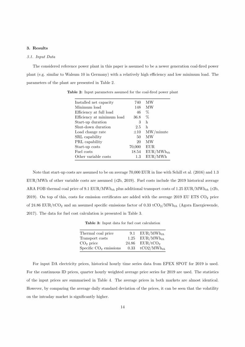
3.3. Dispatch with TES

In this section, the optimal dispatch of the reference coal-fired plant with TES is simulated. The analysis

includes two TES variants: A reference TES whose parameters are derived from the TES specifications stated

in Richter et al. (2019) and a similar TES but with a higher round-trip efficiency.The discharging power of

the high-efficiency TES at full load is adjusted accordingly to reflect the higher efficiency and the charging

power at full load is increased proportionally. The parameters of both TES types are presented in Table 6.

Charging and discharging power of the TES depends on at which plant load level the TES is charged and

discharged, respectively. The discharging power is less than the charging power due to efficiency losses.

Further, note that discharging power of the TES at minimum plant load is very restricted.14 This variation

in the charging and discharging power is included in the model as a linear function of plant load level.

Table 6: Technical parameters of the analysed TES systems

Plant Charging Discharging Avg. round-tripload power (MW) power (MW) efficiency

Reference TES20% 51.8 6.7

61.4%100% 37.0 31.8

High-efficiency TES20% 51.8 6.7

85.0%100% 51.2 44.0

The optimal dispatch for the reference TES with 2 hours of storage capacity at charging power is plotted

in Figure 2 for a representative day. On this particular day (January 16th, 2019) the TES is active on all four

markets (DA, PRL, SRL and ID). The figure of the plant dispatch with TES shows the generator output

(without control power activation), the intraday volumes bought and sold by charging and discharging the

TES, and the control power volumes bid by the plant and those provided by the TES. The second figure

below plots the TES load and stored energy, where the charging and discharging power on day-ahead and

intraday markets and the corresponding energy level can be seen. Note that the stored energy level includes

the activation probability of SRL provision. In these figures it can be seen that the TES is used to provide

PRL and negative SRL during time periods when the price spreads are not profitable for energy arbitrage. In

the periods when spreads are profitable the TES is charged and discharged accordingly to engage in energy

arbitrage on DA and ID markets. Since the amount of profitable spreads are determined by the round-trip

efficiency of the TES, TES systems with higher efficiencies can result in increased energy arbitrage. A

dispatch example that illustrates this effect is provided in Appendix B for the high-efficiency TES.

14For more information on technical characteristics of charging and discharging powers see Richter et al. (2019).

16

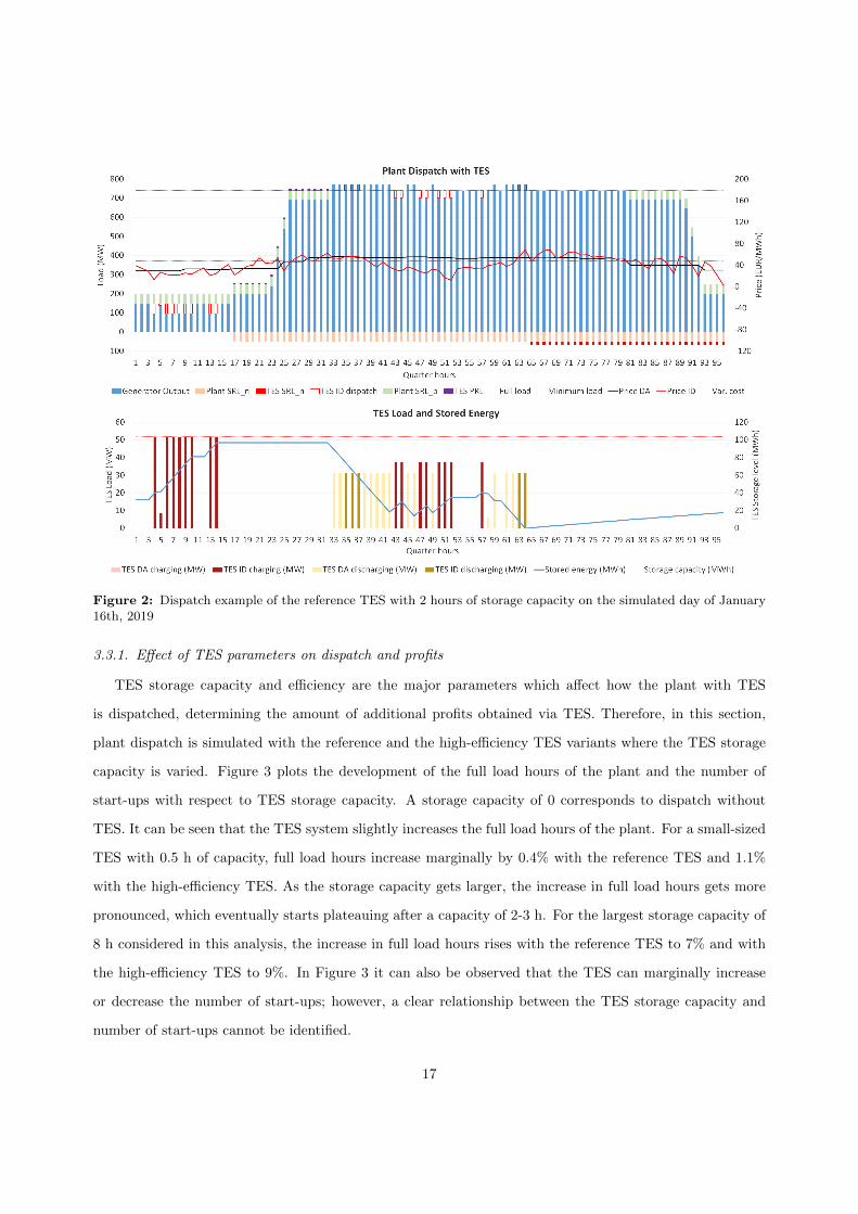
Figure 2: Dispatch example of the reference TES with 2 hours of storage capacity on the simulated day of January16th, 2019

3.3.1. Effect of TES parameters on dispatch and profits

TES storage capacity and efficiency are the major parameters which affect how the plant with TES

is dispatched, determining the amount of additional profits obtained via TES. Therefore, in this section,

plant dispatch is simulated with the reference and the high-efficiency TES variants where the TES storage

capacity is varied. Figure 3 plots the development of the full load hours of the plant and the number of

start-ups with respect to TES storage capacity. A storage capacity of 0 corresponds to dispatch without

TES. It can be seen that the TES system slightly increases the full load hours of the plant. For a small-sized

TES with 0.5 h of capacity, full load hours increase marginally by 0.4% with the reference TES and 1.1%

with the high-efficiency TES. As the storage capacity gets larger, the increase in full load hours gets more

pronounced, which eventually starts plateauing after a capacity of 2-3 h. For the largest storage capacity of

8 h considered in this analysis, the increase in full load hours rises with the reference TES to 7% and with

the high-efficiency TES to 9%. In Figure 3 it can also be observed that the TES can marginally increase

or decrease the number of start-ups; however, a clear relationship between the TES storage capacity and

number of start-ups cannot be identified.

17

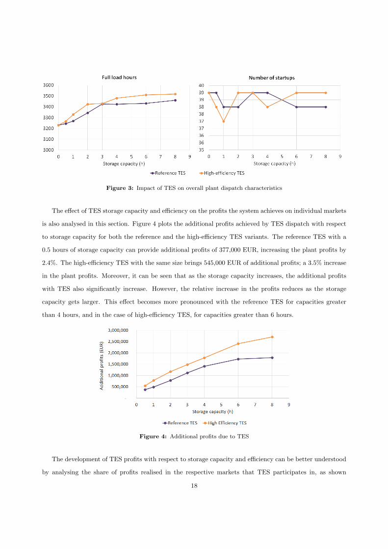
Figure 3: Impact of TES on overall plant dispatch characteristics

The effect of TES storage capacity and efficiency on the profits the system achieves on individual markets

is also analysed in this section. Figure 4 plots the additional profits achieved by TES dispatch with respect

to storage capacity for both the reference and the high-efficiency TES variants. The reference TES with a

0.5 hours of storage capacity can provide additional profits of 377,000 EUR, increasing the plant profits by

2.4%. The high-efficiency TES with the same size brings 545,000 EUR of additional profits; a 3.5% increase

in the plant profits. Moreover, it can be seen that as the storage capacity increases, the additional profits

with TES also significantly increase. However, the relative increase in the profits reduces as the storage

capacity gets larger. This effect becomes more pronounced with the reference TES for capacities greater

than 4 hours, and in the case of high-efficiency TES, for capacities greater than 6 hours.

Figure 4: Additional profits due to TES

The development of TES profits with respect to storage capacity and efficiency can be better understood

by analysing the share of profits realised in the respective markets that TES participates in, as shown

18

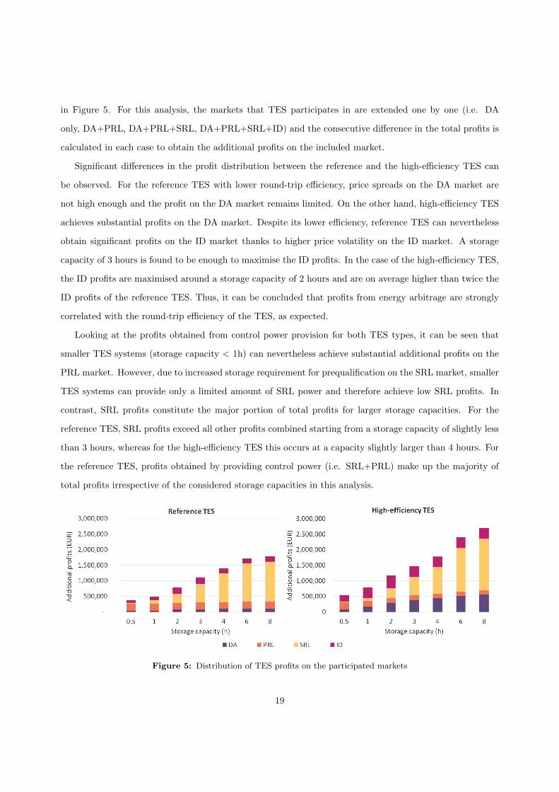
in Figure 5. For this analysis, the markets that TES participates in are extended one by one (i.e. DA

only, DA+PRL, DA+PRL+SRL, DA+PRL+SRL+ID) and the consecutive difference in the total profits is

calculated in each case to obtain the additional profits on the included market.

Significant differences in the profit distribution between the reference and the high-efficiency TES can

be observed. For the reference TES with lower round-trip efficiency, price spreads on the DA market are

not high enough and the profit on the DA market remains limited. On the other hand, high-efficiency TES

achieves substantial profits on the DA market. Despite its lower efficiency, reference TES can nevertheless

obtain significant profits on the ID market thanks to higher price volatility on the ID market. A storage

capacity of 3 hours is found to be enough to maximise the ID profits. In the case of the high-efficiency TES,

the ID profits are maximised around a storage capacity of 2 hours and are on average higher than twice the

ID profits of the reference TES. Thus, it can be concluded that profits from energy arbitrage are strongly

correlated with the round-trip efficiency of the TES, as expected.

Looking at the profits obtained from control power provision for both TES types, it can be seen that

smaller TES systems (storage capacity < 1h) can nevertheless achieve substantial additional profits on the

PRL market. However, due to increased storage requirement for prequalification on the SRL market, smaller

TES systems can provide only a limited amount of SRL power and therefore achieve low SRL profits. In

contrast, SRL profits constitute the major portion of total profits for larger storage capacities. For the

reference TES, SRL profits exceed all other profits combined starting from a storage capacity of slightly less

than 3 hours, whereas for the high-efficiency TES this occurs at a capacity slightly larger than 4 hours. For

the reference TES, profits obtained by providing control power (i.e. SRL+PRL) make up the majority of

total profits irrespective of the considered storage capacities in this analysis.

Figure 5: Distribution of TES profits on the participated markets

19

3.3.2. Charging and discharging patterns

In contrast to the perfect foresight assumption in this paper, dispatching the TES system with the coal-

fired power plant would occur in reality under imperfect information and price uncertainty. This requires

the plant dispatch with charging and discharging instances of the TES to be planned according to forecasts

and would deviate from the optimal results. In this respect, analysing the optimal dispatch simulation

and identifying patterns in charging and discharging instances at respective plant load levels would support

developing TES dispatch strategies.

Figure 6 illustrates the distribution of charging and discharging instances at different plant load levels

for the reference TES with respect to storage capacity. For this analysis, plant load is considered in four

levels of equal load range and any instances, where TES is charging or discharging in these load levels, are

summed up. The overwhelming majority of TES activity (i.e. charging or discharging) is found to occur

close to plant minimum load (20–40% load range) and around plant full load (80–100% load range), while

TES activity in the mid ranges (40–80% load range) is very limited.

The majority of charging occurs around minimum load while the majority of discharging occurs around

full load. This is as expected since—assuming no control power is provided—the plant would run at minimum

load during low electricity prices that lie below its variable costs and would run at full load during higher

profitable prices. Nevertheless, both the ratio of charging around full load and the ratio of discharging

around minimum load increase as the storage capacity gets smaller. For small TES capacities (<1h) these

occurrences are very substantial. With the 0.5 h capacity TES, about 40% of the total charging instances

occur near full load and almost 30% of discharging takes place near minimum load. This is because the

smaller storage capacity restricts the arbitrage potential between minimum load and full load periods where

the absolute spreads are highest, and instead, forces more of the arbitrage to be made in shorter intervals

on constant load levels.

20

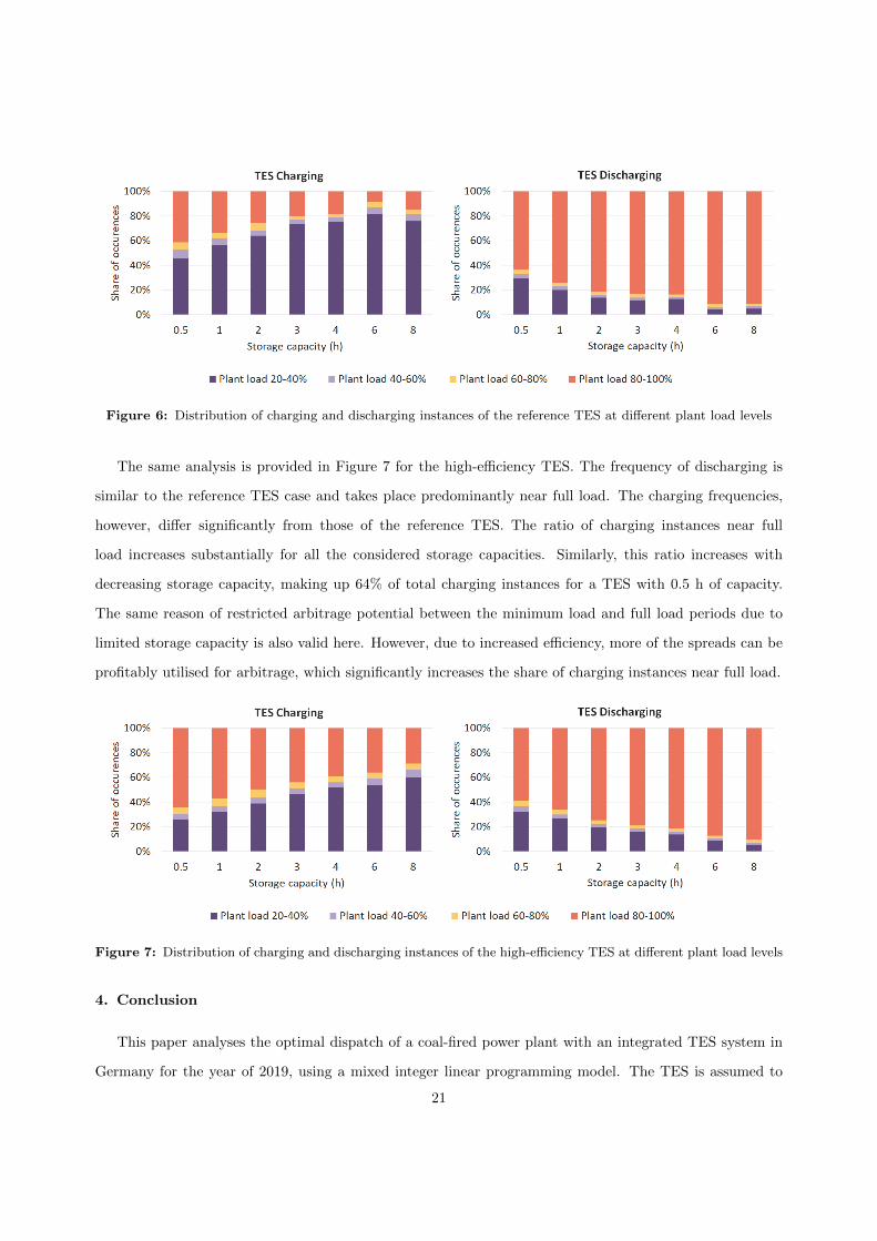
Figure 6: Distribution of charging and discharging instances of the reference TES at different plant load levels

The same analysis is provided in Figure 7 for the high-efficiency TES. The frequency of discharging is

similar to the reference TES case and takes place predominantly near full load. The charging frequencies,

however, differ significantly from those of the reference TES. The ratio of charging instances near full

load increases substantially for all the considered storage capacities. Similarly, this ratio increases with

decreasing storage capacity, making up 64% of total charging instances for a TES with 0.5 h of capacity.

The same reason of restricted arbitrage potential between the minimum load and full load periods due to

limited storage capacity is also valid here. However, due to increased efficiency, more of the spreads can be

profitably utilised for arbitrage, which significantly increases the share of charging instances near full load.

Figure 7: Distribution of charging and discharging instances of the high-efficiency TES at different plant load levels

4. Conclusion

This paper analyses the optimal dispatch of a coal-fired power plant with an integrated TES system in

Germany for the year of 2019, using a mixed integer linear programming model. The TES is assumed to

21

be able to conduct energy arbitrage on the hourly day-ahead and the quarter hourly continuous intraday

markets. Moreover, it can enhance primary and secondary control power provision. In this context, the

effects of TES on the dispatch characteristics of the plant is investigated and additional profits due to TES

are calculated. The relevance of individual TES parameters regarding the profit potential on the respective

markets is shown and charging/discharging patterns are identified.

I find that smaller TES systems (storage capacity ≤ 1 h) achieve substantial profits (about 230,000

EUR) on the PRL market by providing additional PRL flexibility and can also realize significant profits

from energy arbitrage on intraday market (up to about 115,000 EUR) thanks to the more volatile price

structure. Increasing the round-trip efficiency of the TES system can allow a higher share of profits to be

realised also on the day-ahead market and greatly increase total gains via energy arbitrage. I also show that

a storage capacity of 2–3 h is enough to exploit most of the energy arbitrage potential. However, further

increasing the storage capacity enhances profits on the SRL market. I find that the TES system with lower

round-trip efficiency is predominantly charged close to minimum plant load and discharged near full load

because of the limited availability of profitable price spreads due to low efficiency. With higher efficiency,

charging near plant full load becomes more common as the number of profitable spreads increases.

The analysis shows that the TES systems increase the full load hours of the power plant. This increase

can especially be significant for large TES systems, meaning that TES systems can also increase the CO2

emissions of the individual plants. Despite that, the net effects on the system would depend on the specific

CO2 emissions of other technologies which provide similar type of flexibility to the system. As such,

increasing the flexibility potential of conventional power plants via TES can nevertheless help integrating

significant shares of renewables in the medium term. As noted also by Agora Energiewende (2017),

countries with few other flexibility options and large share of inflexible conventional plants such as Poland

and South Africa can especially benefit from the additional flexibility.

The analysis conducted in this paper shows only the energy arbitrage and control power provision

potential of the TES. However, TES can also be used to provide other types of flexibility. For instance, TES

can provide additional heat during start-up in order to reduce start-up time and costs. TES systems can

also be integrated into combined heat and power plants that provide district heating, providing additional

flexibility between the heating and the electricity market. Those aspects can be considered in future research

by extending the presented model. The existing modelling framework assumes perfect foresight and provides

an upper benchmark. For a more realistic dispatch and profit simulation under imperfect information, the

model could be extended with stochastic components to account for price uncertainty. This paper does not

22

provide assumptions or modelling regarding the costs of TES investment and integration of the TES into

the plant. In future research, the analysis could also be extended to take these costs also into account in

order to evaluate the profitability of the investment.

Acknowledgements

I am grateful to Marc Oliver Bettzuge for the valuable input and guidance. Furthermore, I would

like to thank Eglantine Kunle, Max Schonfisch and Johannes Wagner for their helpful comments. The

model developed in this paper benefited from the project “FLEXI-TES - Kraftwerksflexibilisierung durch

thermische Energiespeicher” funded by the German Federal Ministry for Economic Affairs and Energy

(BMWi).

23

References

AG Energiebilanzen, 2020. Stromerzeugung nach Energietragern 1990 - 2019. Available at: https://www.ag-energiebilanzen.de/(Accessed: 18 August 2020).

Agora Energiewende, 2017. Flexibility in thermal power plants - With a focus on existing coal-fired power plants. TechnicalReport.

Arcos-Vargas, A., Canca, D., Nunez, F., 2020. Impact of battery technological progress on electricity arbitrage: An applicationto the Iberian market. Applied Energy 260, 114273.

Beiron, J., Montanes, R.M., Normann, F., Johnsson, F., 2020. Combined heat and power operational modes for increasedproduct flexibility in a waste incineration plant. Energy 202, 117696.

Bradbury, K., Pratson, L., Patino-Echeverri, D., 2014. Economic viability of energy storage systems based on price arbitragepotential in real-time U.S. electricity markets. Applied Energy 114, 512–519.

Cao, R., Lu, Y., Yu, D., Guo, Y., Bao, W., Zhang, Z., Yang, C., 2020. A novel approach to improving load flexibility ofcoal-fired power plant by integrating high temperature thermal energy storage through additional thermodynamic cycle.Applied Thermal Engineering 173, 115225.

Dufo-Lopez, R., 2015. Optimisation of size and control of grid-connected storage under real time electricity pricing conditions.Applied Energy 140, 395–408.

ENTSO-E Transparency Platform, 2020. Available at: https://transparency.entsoe.eu/ (Accessed: 14 September 2020).Eser, P., Singh, A., Chokani, N., Abhari, R.S., 2016. Effect of increased renewables generation on operation of thermal power

plants. Applied Energy 164, 723–732.Evans, A., Strezov, V., Evans, T.J., 2012. Assessment of utility energy storage options for increased renewable energy

penetration. Renewable and Sustainable Energy Reviews 16, 4141–4147.Frangioni, A., Gentile, C., Lacalandra, F., 2009. Tighter Approximated MILP Formulations for Unit Commitment Problems.

IEEE Transactions on Power Systems 24, 105–113.Hentschel, J., Babic, U., Spliethoff, H., 2016. A parametric approach for the valuation of power plant flexibility options. Energy

Reports 2, 40–47.Hong, L., Lund, H., Moller, B., 2012. The importance of flexible power plant operation for Jiangsu’s wind integration. Energy

41, 499–507.Hubel, M., Prause, J.H., Gierow, C., Hassel, E., Wittenburg, R., Holtz, D., 2018. Evaluation of Flexibility Optimization for

Thermal Power Plants, in: Proceedings of the ASME 2018 Power Conference, American Society of Mechanical Engineers,Lake Buena Vista, Florida, USA.

IEA, 2019. World Energy Outlook 2019. Technical Report. International Energy Agency, Paris.Kazempour, J., Yousefi, A., Zare, K., Moghaddam, M.P., Haghifam, M., Yousefi, G., 2008. A MIP-based optimal operation

scheduling of pumped-storage plant in the energy and regulation markets, in: 2008 43rd International Universities PowerEngineering Conference, IEEE, Padova. pp. 1–5.

Knaut, A., Obermuller, F., Weiser, F., 2017. Tender Frequency and Market Concentration in Balancing Power Markets.Technical Report. Institute of Energy Economics at the University of Cologne (EWI).

Knaut, A., Paschmann, M., 2017. Decoding Restricted Participation in Sequential Electricity Markets. Technical Report.Institute of Energy Economics at the University of Cologne (EWI).

Kubik, M., Coker, P., Barlow, J., 2015. Increasing thermal plant flexibility in a high renewables power system. Applied Energy154, 102–111.

Kunle, E., 2018. Incentives to value the dispatchable fleet’s operational flexibility across energy markets. Dissertation.Technische Universitat Clausthal. URL: https://dokumente.ub.tu-clausthal.de/servlets/MCRFileNodeServlet/

clausthal_derivate_00000445/Db113818.pdf.Li, D., Hu, Y., He, W., Wang, J., 2017. Dynamic modelling and simulation of a combined-cycle power plant integration with

thermal energy storage, in: 2017 23rd International Conference on Automation and Computing (ICAC), IEEE, Huddersfield,United Kingdom. pp. 1–6.

Li, D., Wang, J., 2018. Study of supercritical power plant integration with high temperature thermal energy storage for flexibleoperation. Journal of Energy Storage 20, 140–152.

Metz, D., Saraiva, J.T., 2018. Use of battery storage systems for price arbitrage operations in the 15- and 60-min Germanintraday markets. Electric Power Systems Research 160, 27–36.

Musgens, F., Ockenfels, A., Peek, M., 2014. Economics and design of balancing power markets in Germany. InternationalJournal of Electrical Power & Energy Systems 55, 392–401.

Ostrowski, J., Anjos, M.F., Vannelli, A., 2012. Tight Mixed Integer Linear Programming Formulations for the Unit CommitmentProblem. IEEE Transactions on Power Systems 27, 39–46.

r2b, 2019. Flexibility in thermal power plants - With a focus on existing coal-fired power plants. Technical Report. r2b energyconsulting GmbH, Consentec GmbH, Fraunhofer ISI, TEP Energy GmbH.

Richter, M., Mollenbruck, F., Obermuller, F., Knaut, A., Weiser, F., Lens, H., Lehmann, D., 2016. Flexibilization of steampower plants as partners for renewable energy systems, in: 2016 Power Systems Computation Conference (PSCC), IEEE,Genoa, Italy. pp. 1–8.

Richter, M., Oeljeklaus, G., Gorner, K., 2019. Improving the load flexibility of coal-fired power plants by the integration of athermal energy storage. Applied Energy 236, 607–621.

Risthaus, K., Madlener, R., 2017. Economic Analysis of Electricity Storage Based on Heat Pumps and Thermal Storage Unitsin Large-Scale Thermal Power Plants. Energy Procedia 142, 2816–2823.

24

Scapino, L., De Servi, C., Zondag, H.A., Diriken, J., Rindt, C.C.M., Sciacovelli, A., 2020. Techno-economic optimization of anenergy system with sorption thermal energy storage in different energy markets. Applied Energy 258, 114063.

Schill, W.P., Pahle, M., Gambardella, C., 2016. On Start-Up Costs of Thermal Power Plants in Markets with Increasing Sharesof Fluctuating Renewables. SSRN Electronic Journal .

Sioshansi, R., Denholm, P., 2010. The Value of Concentrating Solar Power and Thermal Energy Storage. IEEE Transactionson Sustainable Energy 1, 173–183.

Sioshansi, R., Denholm, P., Jenkin, T., Weiss, J., 2009. Estimating the value of electricity storage in PJM: Arbitrage and somewelfare effects. Energy Economics 31, 269–277.

Swider, D.J., Weber, C., 2007. The costs of wind’s intermittency in Germany: application of a stochastic electricity marketmodel. European Transactions on Electrical Power 17, 151–172.

Walawalkar, R., Apt, J., Mancini, R., 2007. Economics of electric energy storage for energy arbitrage and regulation in NewYork. Energy Policy 35, 2558–2568.

Wojcik, J., Wang, J., 2017. Technical Feasibility Study of Thermal Energy Storage Integration into the Conventional PowerPlant Cycle. Energies 10, 205.

Zhao, Y., Liu, M., Wang, C., Li, X., Chong, D., Yan, J., 2018a. Increasing operational flexibility of supercritical coal-firedpower plants by regulating thermal system configuration during transient processes. Applied Energy 228, 2375–2386.

Zhao, Y., Wang, C., Liu, M., Chong, D., Yan, J., 2018b. Improving operational flexibility by regulating extraction steamof high-pressure heaters on a 660 MW supercritical coal-fired power plant: A dynamic simulation. Applied Energy 212,1295–1309.

25

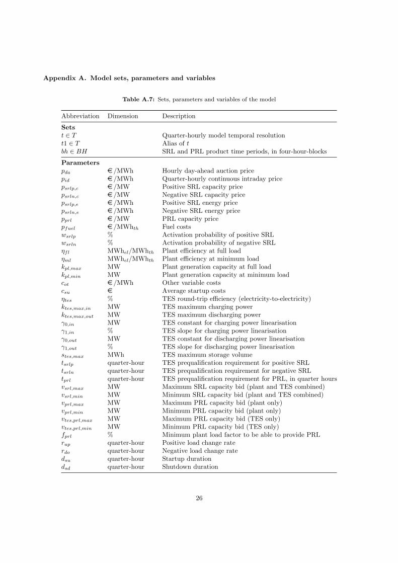
Appendix A. Model sets, parameters and variables

Table A.7: Sets, parameters and variables of the model

Abbreviation Dimension Description

Setst ∈ T Quarter-hourly model temporal resolutiont1 ∈ T Alias of tbh ∈ BH SRL and PRL product time periods, in four-hour-blocks

Parameterspda e /MWh Hourly day-ahead auction pricepid e /MWh Quarter-hourly continuous intraday pricepsrlp,c e /MW Positive SRL capacity pricepsrln,c e /MW Negative SRL capacity pricepsrlp,e e /MWh Positive SRL energy pricepsrln,e e /MWh Negative SRL energy pricepprl e /MW PRL capacity pricepfuel e /MWhth Fuel costswsrlp % Activation probability of positive SRLwsrln % Activation probability of negative SRLηfl MWhel/MWhth Plant efficiency at full loadηml MWhel/MWhth Plant efficiency at minimum loadkpl,max MW Plant generation capacity at full loadkpl,min MW Plant generation capacity at minimum loadcot e /MWh Other variable costscsu e Average startup costsηtes % TES round-trip efficiency (electricity-to-electricity)ktes,max,in MW TES maximum charging powerktes,max,out MW TES maximum discharging powerγ0,in MW TES constant for charging power linearisationγ1,in % TES slope for charging power linearisationγ0,out MW TES constant for discharging power linearisationγ1,out % TES slope for discharging power linearisationstes,max MWh TES maximum storage volumetsrlp quarter-hour TES prequalification requirement for positive SRLtsrln quarter-hour TES prequalification requirement for negative SRLtprl quarter-hour TES prequalification requirement for PRL, in quarter hoursvsrl,max MW Maximum SRL capacity bid (plant and TES combined)vsrl,min MW Minimum SRL capacity bid (plant and TES combined)vprl,max MW Maximum PRL capacity bid (plant only)vprl,min MW Minimum PRL capacity bid (plant only)vtes,prl,max MW Maximum PRL capacity bid (TES only)vtes,prl,min MW Minimum PRL capacity bid (TES only)fprl % Minimum plant load factor to be able to provide PRLrup quarter-hour Positive load change raterdo quarter-hour Negative load change ratedsu quarter-hour Startup durationdsd quarter-hour Shutdown duration

26

Abbreviation Dimension Description

Binary variablesBon 1 if the plant is currently onlineBsu 1 if the plant has started upBsd 1 if the plant has shut downBtes,in 1 if the TES is chargingBtes,out 1 if the TES is dischargingBsrlp 1 if the plant is offering positive SRLBsrln 1 if the plant is offering negative SRLBprl 1 if the plant is offering PRLBtes,srlp 1 if the TES is offering positive SRLBtes,srln 1 if the TES is offering negative SRLBtes,prl 1 if the TES is offering PRL

VariablesRda e Total revenue on the day-ahead marketRid e Total revenue on the intraday marketRsrlp e Total revenue on the positive SRL marketRsrln e Total revenue on the negative SRL marketRprl e Total revenue on the PRL marketCvar e Variable costsCsu e Startup costs

Positive VariablesXda MW Total output on the day-ahead market (Plant + TES)Xpl MW Plant output without TESXovermin MW Plant output that is above the minimum loadPLsrlp MW Plant output on the positive SRL marketPLsrln MW Plant output on the negative SRL marketPLprl MW Plant output on the PRL marketTESda,in MW TES charging on the day-ahead marketTESda,out MW TES discharging on the day-ahead marketTESid,in MW TES charging due to buying back on the intraday marketTESid,out MW TES discharging on the intraday marketTESsrlp MW TES discharging power marketed on the positive SRL marketTESsrln MW TES charging power marketed on the negative SRL marketTESprl MW TES charging/discharging power marketed on the PRL marketEtes,in MWh Energy flow into TES when chargingEtes,out MWh Energy flow out of the TES when dischargingStes MWh Stored energy in the TES

Note: Unless specified, all the power (MW) and energy (MWh) units are electrical.

27

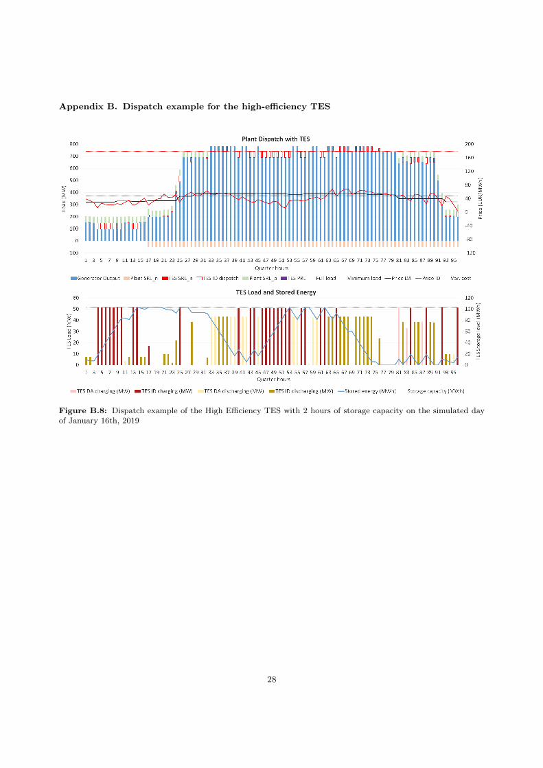
Appendix B. Dispatch example for the high-efficiency TES

Figure B.8: Dispatch example of the High Efficiency TES with 2 hours of storage capacity on the simulated dayof January 16th, 2019

28