optimal design of reliable integrated chemical production sites
TRANSCRIPT

Optimal Design of Reliable Integrated Chemical Production Sites
Sebastian Terrazas-Moreno, Ignacio E. Grossmann*
Chemical Engineering Department Carnegie Mellon University
John M. Wassick, Scott J. Bury The Dow Chemical Company
Rev. July 2010
* Author to whom correspondence should be addressed. Email:
[email protected], Tel: 412-268-3642, Fax: 412-268-7139.

1
Abstract
Since plants that form the network are subject to fluctuations in product demand or
random mechanical failures, design decisions such as adding redundant units and
increasing storage between units can increase the flexibility and reliability of an
integrated site. In this paper, we develop a bi-criterion optimization model that captures
the trade-off between capital investment and process robustness in the design of an
integrated site. Design decisions considered are increases in process capacity,
introduction of parallel units, and addition of intermediate storage. The Mixed-integer
Linear Programming (MILP) formulation proposed in this paper includes the
representation of the material levels in the intermediate storage by means of a
probabilistic model that captures the effects of the discrete, uncertain events. We also
integrate a superstructure optimization with stochastic modeling techniques such as
continuous time Markov chains. The application of the proposed model is illustrated with
two example problems.

2
Introduction
An integrated site consists of a network of plants or large scale processes (Feord, 2002;
Kimm, 2008; Wassick, 2009). The overall objective of the integrated site is to transform
materials supplied from outside of the network into a set of products for which there is an
external demand. The network structure is determined so that intermediate products can
be internally produced by some plants and consumed by others.
Most large-scale chemical integrated sites, such as Dow Texas Operations, have
gradually evolved from smaller sites. The opportunity to design and build completely
new integrated chemical sites has appeared fairly recently. The size and scope of some of
these projects has seldom, if ever, been done before. The risk of integration failures
(mismatch on capacity, blocking or starving other units, etc.) has a much larger downside
than with traditional, independent production plants. Of particular concern is the fact that
uncertain events affect the performance of an integrated site. Some of these are discrete,
such as process failures, while others are continuous, such as variations in external
supply, demand, or fluctuations in plant throughput. Under such uncertain conditions, the
design of integrated sites presents challenges for smooth integration and balancing of
process availability and capacity. Some design decisions can increase the robustness of
the integrated site subject to continuous and discrete uncertainties.
The objective of this work is to develop a systematic method to determine the optimal
trade-off between capital investment and process robustness in the design of an integrated
site subject to discrete and continuous uncertainties. The main design decisions
considered are changes in process capacity, introduction of parallel units, and addition of
intermediate storage. We use a metric known as expected stochastic flexibility E(SF) to
quantify the robustness of the integrated site. E(SF) is a probabilistic measure of the
system’s ability to tolerate continuous and discrete uncertainties (Straub & Grossmann,
1990).
Other authors have studied the problem of addressing reliability or availability of a
process at the design stage. Pistikopoulos et al. (1996) addressed the simultaneous design
and maintenance optimization problem. They introduced a flexibility-reliability index
(FRI) that has the same definition as the expected stochastic flexibility of Straub &
Grossmann (1990). Pistikopoulos et al. (2001) simultaneously solved the production

3
planning and maintenance planning problem for multipurpose batch process plants. They
define system effectiveness as the criterion that balances increased revenues from process
availability improvements and increased maintenance. In a later work, Goel et al. (2003)
extended the system effectiveness approach to incorporate the initial availability of each
process in the system as a degree of freedom. Sherali et al. (2008) studied the optimal
allocation of risk-reduction resources using an event tree representation. Some resources
are used to prevent events in the tree from happening, while others are used to minimize
the loss once the events occur.
Straub & Grossmann (1993) proposed a mathematical formulation for maximizing
stochastic flexibility (SF) at the design level. In this approach, the feasible region is
determined by the choice of the design variables. The stochastic flexibility is
approximated using a set of quadrature points that are placed adaptively inside the
feasible region. This approach requires the solution of a large nonlinear program (NLP).
Bansal et al. (2000, 2002) proposed a parametric programming approach to quantify
stochastic flexibility. The authors derive a set of parametric solutions dependent on
design and uncertain parameters, and a corresponding set of regions where those
solutions are optimal.
Davies and Swartz (2008) studied the effect of intermediate storage on the performance
of a continuous process under random failures. Their approach relies on generating
failure scenarios and optimizing buffer levels over these scenarios using an economic
objective function. Cheng et al. (2003) addressed the problem of design and planning
under uncertainty. Their work is similar to the one presented in this paper in that both
involve multi-objective optimization under uncertainty. They modeled discrete
uncertainties using a Markov decision model where the states of the system depend on
external uncertain conditions (available processing technologies) and internal control
decisions (number of processing units and type of catalyst). A two-stage stochastic
programming problem is solved at each discrete state, where the first stage decisions are
given by the process design, and the second stage decisions are related with production
planning. These authors also included the possibility of modifying the design of the
process in different time periods as more information becomes available. Our work
addresses some points not considered by Cheng et al. (2003). We consider inventory as a

4
way of hedging against uncertainty, and we allow the infeasible operation through the use
of the stochastic flexibility index. Also, the source of uncertainty in our work is both
external (demand and supply) and internal (random unit failures).
The work presented in this paper makes three contributions to the related fields. First, it
proposes a bi-criterion Mixed-integer Linear Programming (MILP) formulation for the
maximization of expected stochastic flexibility E(SF) and minimization of investment
cost. For the evaluation of the expected stochastic flexibility, the basic idea relies on
considering fixed quadrature points and using auxiliary 0-1 variables to determine
feasibility/infeasibility of operation. Second, it integrates the effect of intermediate
storage to the design framework for evaluating and optimizing expected stochastic
flexibility E(SF), a nontrivial task given that no explicit timing considerations are
included in existing formulations for optimizing either the E(SF) or the FRI. The basic
idea here relies on the use of Markov chains and basic random process theory to capture
the discrete-event nature of the problem. Third, in contrast to considering a fixed network
structure as has been done in the past, our work also considers the integration of
superstructure optimization with the Markov chain model of discrete events in the
determination of optimal E(SF). We illustrate our approach with a simple example from
the literature and with an industrial case study. As a result of applying our methodology
to these examples, trade-off curves of optimal expected stochastic flexibility vs. capital
investment are obtained.
Background
Stochastic flexibility
The general mathematical model of a process can be defined as follows:
0),,,( ydxh (1)
0),,,( ydxg (2)
where
x : continuous process variables
d : design variables
: uncertain parameters
y : binary parameter used to include the effect of failures in the processing units.

5
In this work, we only deal with linear equations and inequalities. An example of such a
case is shown in Figure 1 where F corresponds to the feasible region. The contours of the
joint probability distribution for uncertain parameters 1 and 2 are the ellipses in the
figure. The stochastic flexibility (SF) is the cumulative probability of the joint
distribution that lies within the feasible region (Straub & Grossmann, 1990).
Fig. 1 Stochastic flexibility of a feasible region F defined by a set of linear constraints
The size of F is a function of the design variables. In the case of an integrated site;
parallel units, extra capacity additions, and intermediate storage, have the potential to
enlarge the size of F (i.e. operation is feasible for a larger range of uncertain parameter
values).
Stochastic Processes
A stochastic process is a collection of random variables that are all defined on the same
probability space and indexed by a real parameter (Heyman and Sobel, 1982). We denote
a stochastic process by TttX );( , where T is a set of numbers that indexes the random
variable )(tX . For this work, t refers to time and T to the range of times being
considered. In this context, )(tX is the value of the process at time t . When T is finite or
countable infinite, it is said to be discrete; otherwise it is called continuous. The state
space of the process S is the set of possible values for )(tX . We call the values
Ss states. When S contains a finite or countable infinite number of states, it is said to
be discrete, otherwise, it is called continuous. For any state Ss and any time Tt , if
stX )( , we say that the process is in state s at time t . The terms stage and epoch are
sometimes substituted for time, especially in discrete time processes.
FF
1
2

6
Continuous time Markov chain
The stochastic process 0);( ttX is a continuous-time Markov chain with state space
IntegersS if each )(tX assumes values only in S and
nnnnnn itXjtXPitXitXjtXP )(|)()(,...,)(|)( 1001 (3)
where P represents the probability of the event inside the brackets. The conditional
probability notation BAP means the probability of A given B . This is the memory
less property; that is, the future states of a system are independent of all past states except
for the immediately preceding one (Billinton and Allan, 1992).
Availability problems in process networks subject to random failures can be modeled as
continuous time Markov chains. The state space of these systems is made up of all the
different combinations of failures in the network. Each one of these combinations is
called a discrete state. For example, a two processing unit network is subject to random
failures that can completely shut down each of the two units. Failure 1 ( 1F ) affects the
first unit and failure 2 ( 2F ) the second. The state space of the system is
2121 ,,, FandFFFno failureS ; each of the elements in S is a state. The system
transitions between states when a failure occurs or when a failure is repaired. In
continuous Markov chains, each transition is described by a rate. The probability that the
system transitions from the )(no failure state to the ( 2F ) state depends on the probability
of failure of the second unit. When the failure probability is described by an exponential
distribution, then the failure rate of that distribution corresponds to the transition rate
from the )(no failure state to the ( 2F ) state. Figure 2 shows a useful way of representing
the continuous time Markov chain by means of a state space diagram and its
corresponding transitions. If the states of a system and the rates of transition between
them are specified (failure and repair rates), we can use straightforward and well known
“frequency” and “duration” techniques to obtain important information about the system
(Billinton and Allan, 1992). Namely, for state s , we can calculate the long term
probability ( sprob ) of finding the state, mean residence time ( smrt ), frequency of
encounters ( sfr ), and the cycle time for the reappearance of the state ( stc ). We illustrate
these techniques for the two-unit system in Figure 2.

7
Fig. 2 Space state diagram for a two component system
Suppose the two units in the system are subject to one type of random failure that shuts
them down completely. The time to failure mTTF and time to repair mTTR for each unit
m are probabilistic quantities that follow an exponential distribution. As part of the
reliability data of the system we are given the mean time to failure mMTTF and mean
time to repair mMTTR . The failure rate m and repair rate m that characterize the
exponential distributions are the reciprocals of the mMTTF and mMTTR respectively.
The repair rate represents the total number of repairs divided by the total down time. The
equations that allow us to calculate sprob , smrt , sfr , and stc from the knowledge of the
possible system states (Figure 2) and the transition rates between them ( m and m ), as
presented by Billinton and Allan (1992), are as follows.
The probability of finding any unit m in a failed state is mm
m
mm
m
MTTFMTTR
MTTR
,
and the probability of finding it active is mm
m
mm
m
MTTFMTTR
MTTF
. The states in
Figure 2 involve combinations of failed and active units. The probability of finding each
of the states in the figure can be calculated by independent combinations, as shown
below:
1NO failure
3Failure
2
4
2
1
1
2 2
1
1
2 2
: failure rate
: repair rate
Failure 1
Failures 1 AND 2

8
))(( 2211
211
prob (4-1)
))(( 2211
212
prob (4-2)
))(( 2211
213
prob (4-3)
))(( 2211
214
prob (4-4)
The frequency of encountering each state s , sfr , is calculated as the probability of
finding s , sprob , times the rate of departure from s . The rate of departure is the
summation of all the rates that leave the state. For instance, the rate of departure from
state 1 in Figure 2 is 1 + 2. Thus,
)())(( 21
2211
211
fr (5-1)
)())(( 21
2211
212
fr (5-2)
)())(( 21
2211
213
fr (5-3)
)())(( 21
2211
214
fr (5-4)
The cycle time between individual states ( stc ) is the reciprocal of the frequency of
encounters:
ss
frtc
1 (6)
Finally, the mean duration or residence time in state s ( smrt ) is calculated as the
probability of finding s divided by the frequency of encounters:
s
ss
fr
probmrt (7)
Problem Definition

9
The problem that we address in this paper can be stated as follows. We are given
a set of finished products with a demand that is either deterministic, or given by a
specified probability distribution. The raw materials and the intermediate products
involved in the integrated production site are known. The supply of raw material can also
be deterministic, or given by a specified probability distribution. There are a
predetermined number of steps involved in the transformation of raw materials to
intermediate and finished products. Each of these steps is carried out by a different plant
that can have multiple production units. Plants are connected through the flow of
intermediate products between them. The network formed by the plants and their
connections represents an integrated site as shown in the example in Figure 3.
Fig. 3 Integrated Site for the production of Products C and F.
The plants in the integrated site are subject to random failures that result in corrective
maintenance. As a result, plants experience some amount of down time during which
production is decreased or stopped all together. Since plants are interconnected in the
integrated site, a failure event will propagate downstream or upstream, forcing some
other plants to decrease or stop their production. In Figure 4 the dotted lines correspond
to the flows that are affected by the failure of Plant 4. If these events are not considered
while designing the integrated site, there is a risk that product demand will not be
consistently met.
Fig. 4 Propagation of a plant failure in an integrated site
Plant 1
Plant 2 Plant 4 Plant 5
Plant 3
External Demand
External Demand
Intermediate A
IntermediateB
Product C
Intermediate D
IntermediateE
Product F
External Supply
External Supply
Plant 1
Plant 2 Plant 4 Plant 5
Plant 3
Intermediate A
Intermediate B
Product C
Intermediate D
IntermediateE
Product F

10
We consider three types of design variables that have an impact on the flexibility and
reliability of an integrated site. These variables are the sizing of intermediate storage, the
potential addition of parallel production units to each plant, and the increase of plant
capacities. Figures 5 and 6 illustrate addition of parallel units and intermediate storage.
Fig. 5 Process redundancies
Fig. 6 Intermediate storage between plants in the network
A well designed integrated site maximizes the probability of consistently meeting the
production requirements for a fixed available capital investment.
The problem can be stated more precisely as follows.
We are given:
The superstructure of an integrated site with all allowable parallel production
units in each plant and intermediate storage tanks.
A set of materials that the plants consume and produce.
Mass balance coefficients for all units in the superstructure.
Base processing capacity and a range for extra capacity increments for each unit.
Supply of raw materials and demand for finished products (constant or described
by a probability distribution).
Plant 4aIntermediate E
Plant 4bIntermediate E
Intermediate A
Intermediate D
Intermediate B
Plant 4aIntermediate E
Plant 4bIntermediate E
Intermediate A
Intermediate D
Intermediate B
Plant 1
Plant 2 Plant 4 Plant 5
Plant 3Intermediate
A
Intermediate B
Intermediate D
Intermediate E
Product F
Product C
11
Number of failures, associated production rate reductions, and the mean time to
failure MTTF and mean time to repair MTTR that completely specify the
exponential distributions of failure and repair times.
A set of frequency and duration equations that allows us to calculate the cycle
time tc , mean residence time mrt , and frequency of encounters fr , for all the
possible states in the system, based only on the knowledge of the MTTR and
MTTF of the units in the superstructure (Billinton and Allan, 1992). These
equations were explained in the background section of this paper.
A continuous range of tank sizes for intermediate storage.
A cost function that relates design decisions with capital investment.
The problem is to determine:
For each plant, the number of production units.
For each plant, the capacity increment for each unit above the base capacity.
Sizes of intermediate storage between plants.
Subject to:
Mass balances.
Process specifications.
Bounds on production capacity and tank sizes.
The objective is to determine the set of Pareto-optimal solutions that:
Maximize the expected stochastic flexibility.
Minimize the capital investment.
The following assumptions and simplifications are made:
1. Unplanned down time is the result of random and independent failure events.
2. TTF and TTR have exponential distributions. In the case that TTR follows a normal
distribution the Markov chain approach is no longer rigorously valid. However, we
claim that the Markov chain model is a useful approximation for analyzing the long
term behavior of the Integrated Site. We quote Billinton & Allan (1992) on this point:
“It has been stressed […] that, although the assumption of exponential distributions
may have been made, the results and equations are equally applicable to all

12
distributions if only the limiting state or long term average values are being
evaluated for systems containing statistically independent components.”
3. Preventive maintenance is not included.
4. The design cost function is linear.
5. Each plant can be modeled in terms of one output product. The production of all other
products is proportional to the main output. Mass balance coefficients can be used to
specify that the main product can only use a fraction of the total plant capacity.
Maximizing the expected stochastic flexibility and minimizing the capital investment
yields a bi-criterion optimization problem. The results of this bi-criterion optimization in
the form of a Pareto-optimal curve can be obtained by maximizing the E(SF) for various
fixed values of capital investment (i.e. -constrained method (Ehrgott, 2005)).
Mathematical model
Maximization of expected stochastic flexibility
In the background section, we reviewed the concept of stochastic flexibility (SF).
In this section, we introduce expected stochastic flexibility E(SF) as presented by Straub
and Grossmann (1990). We then describe our new approach to maximizing E(SF) in
process systems. For the sake of simplicity in the notation, we use only two uncertain
parameters ( 1 , 2 ) described by a joint probability distribution j( 1 , 2 ). The two
uncertain parameters will be discretized using ),...2,1( 111 Kkk and
),...2,1( 222 Kkk quadrature points. Any point in the ( 1 , 2 ) space is described by a pair
( 21,kk ), where 1k and 2k denote the indices of the quadrature points for 1 and 2
respectively.
Discrete uncertainties related to possible failures of the production units are
captured through the discrete states ),...,2,1( Sss . Each discrete state is described by a
set of failures in the processing units in the system. Mathematically this is represented by
the binary parameter vector sy that has as many elements as the total number of possible

13
failures in all the units of the system. A zero value in a certain position of the sy vector
denotes that a failure is present or occurring when the system is in discrete state s .
Equations (1) and (2) describe a general process model. These equations can be written
for each point ( 21,kk ) and each discrete state s :
0),,,,(22112121 s
kk
skk
skk ydxh (8)
0),,,,(22112121 s
kk
skk
skk ydxg (9)
We introduce a non-negative slack variable u , and a binary variable w associated with
each discrete point ( 21,kk ) in each state s . If the point ( 21,kk ) lies inside the feasible
region corresponding to state s , the binary variable skkw 2,1 takes a value of one and the
slack is zero as given by equations (10) - (14). Infeasibility leads to a nonzero slack,
which in turn removes inequality (12). The parameter M in equation (12) corresponds to
a valid upper bound for the left hand side of equation (11).
For each
11 ,...2,1 Kk ; 22 ,...2,1 Kk ; Ss ,...,2,1
we have:
0),,,(21 212121 ss
kks
kk ydxhkk
(10)
skk
sskk
skk uydxg
kk 21212121 ),,,(21
(11)
)1( 2121s
kks
kk wMu (12)
021 skku (13)
}1,0{21 skkw (14)
Assuming a given quadrature formula for approximating the integral in the stochastic
flexibility (e.g. Gaussian quadrature), we calculate the probability 21kk associated with
each point ( 21,kk ) as follows:
),(2
)(
2
)(2211
22112121 kk
LULU
kkkk j
(15)
where i is the weight of the thi quadrature point. Ui
Li , are lower and upper bounds
of the uncertain parameters. Note that these bounds are independent of the feasible

14
region. For instance, normally distributed parameters can be bounded by the average
value minus and plus four standard deviations. ),(21 21 kk
j is the value of the joint
probability distribution at the point ( 21,kk ).
For a given state s , the stochastic flexibility can be computed as:
1
1121
2
1221
K
k
skk
K
k
skk
s wSF (16)
Figure 7 illustrates our approach for calculating the stochastic flexibility.
The objective of maximizing the expected stochastic flexibility E(SF) can now be defined
as follows,
1
1121
2
1221
1
)(maxK
k
skk
K
k
skk
S
s
s wprobSFE (17)
Here sprob is the probability of finding the system in discrete state s after a long time of
operation. sprob can be calculated from the reliability data of the integrated site; it is a
parameter in the optimization formulation. Equation (17) is used as one objective
function for the bi-criterion formulation developed in this work.
Fig. 7 Stochastic flexibility by discretization of uncertain parameters
The formulation described by equations (10) – (14) and (17) results in a problem that
grows exponentially with the number of uncertain parameters and number of elements in
the y vector (i.e., the number of possible failures in the integrated site). Therefore,
algorithmic techniques are required for the solution of large-scale problems with this
FF
1U
2U
1L
2L
wk1,k2 = 0
wk1,k2 = 1
Probability of (k1,k2) point = k1,k2
FF
1U
2U
1L
2L
wk1,k2 = 0
wk1,k2 = 1
Probability of (k1,k2) point = k1,k2

15
formulation. The need to check feasibility for every state and every collocation point
might be avoided by using bounding search procedures (Straub and Grossmann, 1990)
and logic cuts (Hooker et al., 1994). The focus of this paper, however, is the development
of our formulation and its integration with intermediate storage modeling and
superstructure optimization. We will address the solution of large-scale problems in a
future paper.
Integrated site process model
So far we have used a general process model. In this section, we describe the particular
model we use for integrated sites. The continuous process variables x in equations (1)
and (2) are material flows. As seen in Figure 8, the variable ps corresponds to the
process streams that feed the units; the variables f and flow are the remaining flow
variables ( flow are inputs/outputs for each plant, f are internal flows). The design
variables d in (1) and (2) correspond to production unit extra capacity additions pc , the
binary variable associated with installation of a parallel production unit z , the storage
tank volume v and the average inventory level inv . The yield coefficients, the base
processing capacity of each unit, and upper and lower bounds for all variables are
deterministic parameters. The uncertain parameters in (1) and (2) are the raw material
supply RM and demand of finished products DF . In the following section, we describe
the process network model for the integrated site corresponding to equations (8) and (9).
Let Jj ,...,2,1 refer to a set of large-scale chemical processes or plants, and
Nn ,...,2,1 refer to the products consumed and produced by all the plants. The
superstructure of the integrated site considers jMm ,...,2,1 parallel production units for
each plant j . Every plant j has an intermediate storage tank for product n , described
by its total volume njv , and its average inventory level njinv , . Both of these quantities
will take the value of zero if no storage is required. Figure 8 shows the basic building
block for every plant j in the superstructure. We use the variable jf to represent
material flows within the block corresponding to plant j (e.g. the flow from the
production units to the storage tank) and jjflow ,' to represent the flow that goes from

16
plant 'j to plant j . The variable mps stands for processing stream fed to each production
unit m .
Fig. 8 Building block for plant j in the integrated site
Finally, we have a set of Ss ,...,2,1 discrete system states, and sets 11 ,...,2,1 Kk and
22 ,...,2,1 Kk of quadrature points for uncertain parameters 1 and 2 . The following
equations describe the material balance for the building block shown in Figure 8.
22112,1,,'
2,1,,,,' ,,, '
KkKkSsJjpsflowjj jj Mm
kksmFEEDj INPUTOUTPUTn
kksnjj
(18)
2211,
'2,1,,,,'
'2,1,,,,
,,,,,
'
KkKkSsNrefnNnJjflow
flow
jn
nj
FEEDjkksnjj
FEEDjkksnjj
j
j
(19)
22112,1,,,2,1,, ,,,, KkKkSsOUTPUTnJjfps jP
kksnjMm
kksmm
j
(20)
KkKkSsOUTPUTnJjfff jB
kksnjIN
kksnjP
kksnj 2112,1,,,2,1,,,2,1,,, ,,,, (21)
KkKkSsOUTPUTnJjffflow jPRODj
Bkksnj
OUTkknjkksnjj
j
211'
2,1,,,2,1,,2,1,,,', ,,,,
(22)
KkKkSsOUTPUTnJjJjflow jkksnjj 21'2,1,,,,' ,,,,,' 0 (23)
Unit 1
Unit 2
Inter. Tank j
Unit Mj
Sum over all plants j’ that feed plant j
2psPjf
1ps
jFEEDj
jjflow'
,'
......
...
jMps
Bjf
INjf OUT
jf
jPRODj
jjflow'
',
Sum over all plants j’ that receive product from plant j

17
In equation (18) the set jFEED contains all upstream plants that feed material to plant
j . jINPUT and jOUTPUT are subsets of N corresponding to the materials consumed
and produced by plant j . The set jM contains the parallel units m postulated for plant
j . The variable 2,1,,,,' kksnjjflow represents the flow of product n from plant jFEEDj '
to plant Jj , during state s and in quadrature point ( 21,kk ). The variable 2,1,, kksmps
represents the flow supplied to the thm production unit in plant j ( since jMm )
during state s and in the quadrature point ( 21,kk ). In equation (19), nnj , is the mass
balance coefficient for product n in plant j using product n as reference. For example,
if plant 1 consumes two tons of raw material B for each ton of raw material A, then
1,1 AA and 2,1 A
B . The parameter m in equation (20) is the yield coefficient for
production unit m , while the variable Pkksnjf 2,1,,, represents the total flow of product
jOUTPUTn out of the M parallel units in plant j . In equation (21), the flow into the
storage tank is represented by INkksnjf 2,1,,, . The flow that bypasses the storage tank is
represented by Bkksnjf 2,1,,, .
In equation (22), the set jPROD contains all the plants that use the product of plant j .
The variable OUTkksnjf 2,1,,, represents the flow out of the storage tank. The net flow from plant
j to other plants jPRODj ' in the network is 2,1,,,', kksnjjflow .Equation (23) sets equal to
zero the flows of the products n that are not produced by plant 'j .
More constraints can be added for process specifications. The most common of them is
the specification to consume no more than the maximum supply of raw materials and to
produce at least all the finished product that is demanded. These constraints are written
below.
22111,2,1,,,,supplier ,,,RAW supplier
KkKkSsNnRMflow knPRODj
kksnj
(24)
22112,2,1,,,consumer, ,,,FINISHED consumer
KkKkSsNnDFflow knFEEDj
kksnj
(25)

18
The set RAW is a subset of products corresponding to externally supplied raw materials.
The set FINISHED contains the finished products sent to external consumers. The model
considers one external supplier and one external consumer per product n . In practical
problems there might be many suppliers and consumers, but we assume that their
behavior can be summed into one large supplier and one large consumer. The sets
supplierPROD and consumerFEED include the plants that use the externally supplied raw
materials and that feed the external consumer, respectively. The supply of raw material
RAWn to plant j is labeled njflow ,,supplier and the flow of finished product
FINISHEDn from plant j is labeled nj,flow ,consumer .
1,knRM is a parameter that indicates the external supply of n in collocation point k1;
2,knDF is a parameter that indicates the amount of finished product n demanded in
collocation point 2k . The non-negative slack variable skku 2,1 is added to equations (24)
and (25), and the feasibility of the point ),( 21 kk in state s is determined through the use
of the binary variable skkw 2,1 .
2211211,2,1,,,,supplier ,,,RAW upplier
KkKkSsnuRMflow ,ks,kknPRODj
kksnj
s
(26)
22112,1,2,1,,,consumer,2, ,,,FINISHED consumer
KkKkSsnuflowDF kksFEEDj
kksnjkn
(27)
KkKkSswMu skk
skk 2112121 ,, )1( (28)
KkKkSsu skk 2112,1 ,, 0 (29)
KkKkSswskk 21121 ,, }1,0{ (30)
Representation of random failures
Plant Jj in the integrated site can consist of multiple parallel production units
jMm . Let Jj
jMM
be the set of all units in the integrated site. Every unit Mm is
subjected to random failures. Some of them are partial failures that decrease the
production rate, while others are total failures that cause complete unit shutdown. Let
mL,...,2,1l be the different types of random failures that arise in unit m . The set
19
Mm
mLL
contains the possible failures of all the units in the integrated site. Each failure
Ll is characterized by a production rate decrease (or rate cut) lrc , an exponential
distribution for time to failure lTTF , and a normal or exponential distribution for time to
repair lTTR . Recall that in the Problem Definition section we presented the Markov
chain model as a useful approximation of the average behavior of the system for long
operating horizons, even if the lTTR does not follow an exponential distribution. The rate
cut, which ranges between 0 and 1, describes the fraction of the maximum capacity that is
lost during the failure. A rate cut of 1 indicates total failure. All the rate cut information
and distribution parameters are given as part of the reliability data of the units. At any
point in time there can be a combination of failures occurring in the Mm units in the
network. The combination of failures at any instant is called a discrete state of the
integrated site. The set Ss ,...,2,1 , is used to refer to such states. The binary vector sy
has an element for each of the possible failures of each of the production units in the
integrated site. Since a unit can experience more than one type of failure, the vector sy
can have more than one element per production unit. This vector contains a 1 for each
failure that does not occur as part of state s , and a 0 in the position associated with a
failure that occurs as part of state s . Note that sy is a fixed parameter. The next equation
describes the effect of failures on the capacity of the plants in the network:
22112,1,, ,,,, ))(1(1)( KkKkSsLMmrcypcbcps ms
mmkksm lll (31)
2,1,, kksmps represents the flow supplied to the thm production unit during state s and
quadrature point ( 21,kk ). The parameter mbc is the base processing capacity of unit m .
The design variable mpc represents extra capacity additions. The parameter syl is the
value assigned to vector sy in the position corresponding to thl failure in the thm
production unit (since mLl ). Finally, lrc is the rate cut corresponding to failure l .
The long term probability of having failure l in the integrated site at any instant is given
by (Billinton and Allan, 1992):

20
ll
ll MTTFMTTR
MTTRp
(32)
The long term probability of finding the integrated site in state s is given by:
0: 1:
)1(s sy y
s ppprobl ll l
ll (33)
The integrated site is continuously transitioning between discrete states. This behavior is
modeled as a continuous time Markov chain where each state s corresponds to a cycle
time stc , frequency sfr , and mean residence time smrt . As explained in the background
section, all these quantities can be calculated from the MTTR and MTTF of the units in
the integrated site and can be considered given parameters.
Modeling of intermediate storage
The flows in and out of the intermediate storage tank after process j are represented by
the variables INkksnjf 2,1,,, and OUT
kksnjf 2,1,,, . To represent the difference between these flows, we
define the decision variable OUTkksnj
INkksnj
Skknj ff 2,1,,,2,1,,,2,1,, . For the sake of simplicity, in
most of this section we use the notation S , and later use it in full indexed form. The
transitions between discrete states Ss are described by a continuous time Markov
process. The bounds on the feasible rate of depletion or replenishment of the inventory
S during state s depend on the duration of the state, the amount of material in the tank,
and the available storage volume at the beginning of state s . Not all of these quantities
are deterministic. The duration of s follows a probabilistic distribution determined by the
time to repair TTR and time to failure TTF of the units in the integrated site. The
material and available space depend not only on the size of the tank, but also on the
sequence of states that brought the system to state s . Figure 9 shows one possible
trajectory for the system. The x-axis corresponds to time. The points in this axis are those
instants in which the system transitions between states. We will denote these instants
epochs. The y-axis shows the inventory levels as a function of time or epochs. The slope
between epochs i and 1i represents the rate of consumption or replenishment of the
inventory during the state s resided in during the interval ii tt 1 . This interval is also the

21
residence time srt in state s . Note that the states Ss refer to the discrete states of the
continuous time Markov process described by failure and repair events in the integrated
site. The amount of materials iX consumed or accumulated during the interval ii tt 1
while the system is in state s is given by,
iisirtX isisi epoch at state the toingcorrespond )( and , )()( (34)
iX is a random variable since the residence time )(isrt in state )(is , that is ii tt 1 ,
depends on the TTR of the failed units, and the TTF of the active units in state )(is .
Both, TTR and TTF are described by probabilistic distributions. The inventory level at
the time )(qt corresponding to the start of the thq epoch, is given by the following
equation:
1
1
)()(0
1
1
))((q
i
isisq
i
io rtinvXinvqtinv (35)
Note that such a definition of ))(( qtinv involves a summation of random variables,
making ))(( qtinv also a random variable.
Fig. 9 One possible sequence of states and the corresponding inventory levels in an intermediate tank
We now relate the mean inv and standard deviation sd of the inventory level after a
long time of operation ( )(qt ) to the properties of the states Ss known “a priori” -
inv(t)
1 2 3 qq - 1
I(tq)
X0
0
X1X3
Xq-1X2

22
the mean residence time smrt , frequency of encounters sfr , and cycle time stc - and the
values of the decision variables s and 0inv .
Since the expectation of a sum of variables is equal to the sum of its expectations
(Uspensky, 1937), we calculate the mean inventory level as:
1
1
)()(0
1
1
)()( )()())((q
i
isisq
i
isiso mrtinvrtEinvEqinvEinv (36)
where smrt is the mean residence time of state s .
The crucial step that follows is changing the summation over epochs 1,...,2,1 q into a
summation over states s . In this work, we are interested in the stationary behavior of the
system where t . After a long time of operation )(qt , each state will be
encountered tfr s times. In practice, t is a value long enough that allows the Markov
process (of random failures and repairs) to achieve the stationary state. Equations (37)
and (38) will show that the expected inventory level ( inv ) is not sensitive to the exact
value chosen for t . Recall that sfr can be calculated as the probability of finding the
state sprob times the rate of departure from the state. The way in which the frequency
sfr is calculated from the reliability information of the units in the integrated site is
described in detail in the background section. Using this information, equation (36)
becomes:
Ss
ssso tfrmrtinvinv (37)
To make sure that inv remains bounded and kept close to 0inv as )(qt , we add the
following constraint:
0Ss
sss frmrt (38)
Equations (37) and (38) imply that as t , 0invinv . These equations are important
because they relate the amount of inventory consumed or accumulated in each state s as
the plants undergo failure and repair events, to a long term average inventory level. To
incorporate the effect of quadrature points, equation (38) is substituted by the following
two equations:

23
NnJjSsskknj
Kk Kkkk
snj
,, 2,1,,11 22
2,1, (39)
NnJjfrmrtSs
sssnj
, 0, (40)
where 21 ,kk are the indices of the quadrature points of the uncertain parameters (only
two parameters are used for consistency with equations (10) – (14), (17), but the model is
not limited to this number of parameters) and 2,1 kk is the probability of the quadrature
point ( 21 ,kk ). s
nj , is the average rate of consumption or accumulation in the storage
tank during state s . The inventory level, modeled as a random process in equations (35)
– (40), is similar to the well-known model of random walks (Heyman and Sobel, 1982).
In our formulation we have to account for the fact that the “walk”, or in other words the
inventory level, is not unbounded.
We derive the standard deviation sd in an analogous way as the expected inventory
level. Refer to equation (35) and recall that )(tinv is a random variable, and that it
includes a summation where the residence time in each state srt appears. We use the
following definition for the variance of a sum of random variables (Uspensky, 1937) :
ji
jiIi
iIi
i YYCOVARYVARYVAR ),(2)()( (41)
The variables iY correspond to
1
1
)()(q
i
isis
o rtinv . Since the residence times in each
state ( srt ) are independent, the COVAR term in equation (41) is equal to zero, yielding,
)()()(1
1
)(2)(
1
1
)()(
q
i
isisq
i
isisrtVARrtVARinvVAR (42)
We can change the summation over epochs 1,...,2,1 q into a summation over states s as
in equation (37), so that equation (42) becomes:
)()(2
s
Ss
ss rtVARtfrinvVAR
, (43)
It then follows that the standard deviation is:
)())(( invVARqinvsdsd )(2
s
Ss
ss rtVARtfr
. (44)
In order to keep the optimization model linear, we use the following overestimation of sd,

24
~2
)()( sdrtVARtfrrtVARtfrsdSs
ssss
Ss
ss
, (45)
where ss SDrtVAR )( . sSD can be determined from the reliability data of the
integrated site. In the case where the TTF and TTR follow exponential distributions, the
variance of the residence time srt is equal to its mean; that is, ss mrtSD . In the
second numerical example presented in this paper, we use the simplification
ss mrtSD even though the TTR follows a normal distribution. We are aware that this
is not the exact variance for a normal distribution, but given that we are only using
approximate formulas for the variance and standard deviation of the residence time (i.e.,
equation 45) we assume this simplification to be a first approximation to the behavior of
the system.
Recovering the full indices of the decision variables, the equation for determining an
overestimation of the standard deviation of the inventory level ( inv ) as t is given as
follows:
NJ,njtfrSDsdSs
ssnj
snj
,
~
, (46)
Notice that there is a term t in equation (46) that stands for a long time of operation
( t ). In practice we set t equal to the time we expect the integrated site to operate
continuously. A good estimate for t is the time between scheduled maintenance, or any
other major operation interruptions. In the examples presented in a later section, the time
t was set equal to one year of operation. To make sure that the probabilistic distribution
of the inventory after a long time operation ( ttinv ),( ) falls within the physical
bounds of the holding tank, we use the following two equations:
NnJjvsdinv njnjupnj , ,,
~
, (47)
NnJjsdinv njlonj , 0,
~
, (48)
where njv , is the storage capacity of product n in plant j and up and lo are parameters
that truncate the area under the probability distribution of the inventory level ( inv ). If we

25
assume that the inventory level follows a normal distribution we can set 4 loup ,
which leads to a 99.99% probability of the distribution function.
In equation (46), we are using s
that corresponds to the average of skk 2,1 over all
collocation points 1k and 2k , as obtained in equation (39). This average rate of inventory
consumption/replenishment s
could have a moderate value as a result of averaging
large negative (consumption) rates skk 2,1 in some collocation points and large positive
(replenishment) rates in others. For example, s
could be 5 units/hour for a 100 unit tank,
as a result of averaging skk 2,1 =-9,990 and s
kk '2,'1 = 10,000 units/hour in two equally
probable collocation points. In order to constrain the value of skk 2,1 at each collocation
point, we add constraints (49) and (50).
2211,2,1,, ,,,, KkKkSsNnJjvmrtinv njss
kknj (49)
22112,1,, ,,,, 0 KkKkSsNnJjmrtinv sskknj (50)
Finally, the intermediate storage volume is bounded by its maximum capacity:
NnJjvv nj , 0 UBnj,, (51)
Cost function
In this work, we use the linear cost function (52) for minimizing capital investment
required by the integrated site design. Installing a processing unit with its base capacity
has a fixed cost, and a variable cost for the extra capacity addition. The cost associated
with intermediate storage is assumed to vary linearly with the size of the tank.
)( min ,tank,
var
Jj Mm Nn
njnjmmmfix
m
j
vpczcap (52)
In the above objective function, fixm is the fixed cost for including unit m in the
integrated site and varm is the variable cost associated extra capacity addition ( mpc ).
tank,nj is the cost related to the size of the intermediate tank for product n after plant j .
Since the problem is a bi-criterion optimization, the cost function (52) is minimized while
the expected stochastic flexibility in (17) is maximized.

26
Superstructure optimization
In this work, we assume that a superstructure of design alternatives is specified for the
integrated site. The superstructure consists of the network of processes in the site, where
each process is represented by the building block in Figure 8. In order to model the
selection of the optimal design embedded in the superstructure, we define the binary
variables mz that take a value of 1 if the thm production unit is included in the integrated
site and 0 otherwise. This variable is used in following constraint,
22112,1,, ,,,, KkKkSsMmJjMUzps jmkksm (53)
where MU is a valid upper bound for the flow processed by the thm production unit. We
also use the variables mz in the logic cuts (Hooker et al., 1994) given by equations (54)
and (55).
NnJjzvvjMm
mUP
njnj
, ,, (54)
ba m
mmz (55)
Equation (54) allows storage njv , to be built only for those plants j that are part of the
integrated site. The units jMm are the parallel units proposed for plant j in the
superstructure, and the term jMm
mz will be zero if none of these units is part of the
optimal design (i.e. plant j is not part of the integrated site). Equation (55) is a set of
linear inequalities that expresses logical relations on the network topology of the
integrated site in terms of the variables mz .
The complete optimization model is defined by equations (17)-(23), (26)-(31), (39), (40),
(46)-(55), plus constraints (56) and (57) which are introduced in a later section of the
paper. This formulation involves the integration of a state-space model and a
superstructure optimization approach. Most of the problem variables and constraints are
defined for each state and collocation point, therefore, the dimensionality of the
optimization problem grows exponentially with the number of possible failures in the
superstructure and the number of uncertain parameters. Table 1 includes a summary of all
the decision variables included in this problem. Examples 1 and 2 in this paper illustrate

27
the problem sizes that results from applying the proposed formulation to specific
integrated sites.
Table 1 Decision variables in the optimization model
Continuous design variables
Process capacity, mpc
Storage tank capacity njv ,
Average storage level njinv ,
Standard deviation of levels of storage njsd ,
Continuous operation variables
Flow among plants 2,1,,,,' kksnjjflow
Flow from production units Pkksnjf 2,1,,,
Flow into storage tanks INkksnjf 2,1,,,
Flow out of storage tanks OUTkksnjf 2,1,,,
Flow that bypasses the storage tank Bkksnjf 2,1,,,
Accumulation rate in storage Skknj 2,1,,
Average accumulation rate per state Snj ,
Absolute value of accumulation rate Snj ,
Auxiliary continuous variables
Slack variable skku 2,1
Discrete variables
Feasibility variable skkw 2,1
Unit selection variable mz
The integration of the state-space model and the superstructure optimization approach
presents challenges that are not found in standard superstructure optimization problems.
Each possible flowsheet corresponds to a different state space; if unit m is not part of the

28
flowsheet then the failure modes that occur in this unit should not be considered when
deriving the state-space from all the combinations of possible failures in the flowsheet.
For instance, a flowsheet with 4 units, where each unit can be either UP or DOWN, will
have a state-space of cardinality 16. A flowsheet with 10 units will have a state-space of
cardinality 1024. Furthermore, the probability of finding any state in the flowsheet with 4
units will be different (i.e., larger) that finding any state in the flowsheet with 10 units.
The probability of finding state s is sprob in the objective function (17). If sprob
becomes a variable -as it appears to be the case in a superstructure optimization problem-
equation (17) becomes bilinear and nonconvex, destroying the MILP structure of the
problem. Our objective in this part of the paper is to propose an approach where the
probabilities of finding each state sprob and all the other reliability indicators,
sss tcfrmrt ,, , are kept as problem parameters, even if we use a superstructure approach.
In the remainder of this section we present our result, describe it qualitatively, and then
provide rigorous mathematical propositions that validate it.
Our result is the following: we solve the problem defined by equations (17)-(23), (26)-
(31), (39), (40), (46)-(55), plus constraints (56) and (57) defined below, for all the states
Ss resulting from all the potential production units in the superstructure and obtain an
optimal selection of processes that we call M , as will be rigorously proved in the next
section. We claim that this solution (with the complete state space S ) is equivalent to
that obtained by solving the problem starting with just the optimal selection M . It should
be clear that this result is not obvious. The reasons are that when we solve the problem
for the state-space derived from the units in the superstructure we are considering failure
modes and repair actions for units that do not exist in the optimal flowsheet; also, we are
using reliability data ssss tcfrmrtp ,,, of a system that corresponds to all the units in the
superstructure. These data are different form the data corresponding only to the optimal
flowsheet.
',',,','ssSsSsJjzM
Mm
ss
mLm
sj
sj
l
l (56)
',',,','ssSsSsJjzM
Mm
ss
mLm
sj
sj
l
l (57)

29
Before proceeding with the qualitative explanation of the result we describe equations
(56) and (57). Recall that sj is the average rate of consumption or depletion of material
in the intermediate storage tank after plant j during state s . In (56) and (57) M is a valid
upper bound (a big-M), and ss,l is a problem parameter that can be derived form the
vector syl . The vector syl is a fixed parameter defined in a previous section to be 1 if
failure l does not occur as part of state s , and 0 otherwise. Let the parameter ss,l be
defined as follows.
',',,)}1()1(,min{ '' ssSsSsL yyyy sssss,s l lllll (58)
In equation (58) syl is set to one if states s and 's are distinguishable with respect to
failure l ; that is, if the failure occurs in one state and not in the other. Equations (56) and
(57) set the values of sj and
'sj equal for the pairs s and 's that are indistinguishable
with respect to the failures of the m units installed.
To illustrate the main idea behind the result mentioned before, assume there is a
superstructure that consists of 3 units. Each of these units can be in an UP or DOWN
state. Figure 10 shows the different state-spaces that result from different selections of
units from the superstructure.
Fig. 10 State-space representation as a function of the number of units
Our result says that we can optimize over the state-space in the last level of the tree (8
states), even if the optimal flowsheet contains only one or two units. Figure 11a shows
that if only one unit is installed, the four states in the last level of the tree that are derived
},{ DU
)},(),,(
),,(),,{(
DDUD
DUUU
)},,(),...,,,(
),,,(),,,{(
DDDUDU
DUUUUU
State-space for one unit
State-space for two units
State-space for three units
U = Unit upD = Unit down

30
from the same node in the one unit state-space are identical in terms of
feasibility/infeasibility. This figure also shows that the sum of the probabilities of the four
states in the last level of the tree is equal to the probability of the state from which they
are derived in the one unit state-space. Figure 11b shows the equivalent result for the case
where two units are installed.
Fig. 11a Optimization of a flowsheet with one unit using the three unit state-space
Fig. 11b Optimization of a flowsheet with two units using the three unit state-space
Note that the relationships of common feasibility/infeasibility and of the summation of
probabilities appear in our problem without adding any extra constraints except for
equations (56) and (57). In the case illustrated in Figure 11a, equations (56) and (57) set
the rate of consumption/replenishment of inventory s
equal for each of the groups of
FeasibleP = 0.6
InfeasibleP = 0.4
Feas.P = 0.2
Feas.P = 0.1
Feas.P = 0.2
Feas.P = 0.1
Inf.P = 0.1
Inf.P = 0.1
Inf.P = 0.1
Inf.P = 0.1
FeasibleP = 0.3
FeasibleP = 0.2
Feas.P = 0.2
Feas.P = 0.1
Feas.P = 0.2
Feas.P = 0.1
Feas.P = 0.1
Feas.P = 0.1
Inf.P = 0.1
Inf.P = 0.1
FeasibleP = 0.3
InfeasibleP = 0.2

31
four states linked by the doted lines. The reason that explains why these constraints are
needed for the variable s
but not for any of the other variables in the model can be
expressed in a simplified way as follows. The flow variables, flowfps ,, , are zero for
those units that are excluded from the optimal flowsheet by equation (53), regardless of
whether the unit is described as UP or DOWN in the states in the last level of Figure 11a.
However, the variable s
appears in equations (40) and (46) where the duration and the
frequency of appearance of each state are involved. If we use the state-space in the last
level of the tree in Figure 11a, each of the nodes corresponds to a state with a different
duration and frequency so that different feasible rates of consumption/depletion of
inventory can be chosen for each of the states in this level. Equations (56) and (57)
prevent this from occurring. This discussion is formalized in the next subsection.
Properties of the superstructure optimization model
To prove the above claim on the superstructure optimization, we review some
nomenclature and introduce some new sets. Let an integrated site have Jj plants,
where each of them can have jMm parallel production units. The set
j
jMM contains all the candidate production units in the integrated site. Each
Mm is subject to mLl potential failures. The set m
mLL contains all the possible
failures of all the candidate production units in the superstructure of the integrated site.
Recall that each discrete state is a particular combination of failures occurring
simultaneously. The state space S contains all the states resulting from the combination
of the Ll failures that can occur in any of the Mm processing units.
Remark There is a one to one correspondence between a set M and a set L . Also each
set L generates one particular state space S .
Suppose we solve the optimization problem in equations (17)-(23), (26)-(31), (39), (40),
(46)-(57) and find that the optimal solution involves only a subset of the units postulated
in the superstructure; we represent this subset as MM . This means Mmzm ,1
and MMmzm \,0 . The possible failures relevant to the set M are contained in set

32
Mm
mLL
.
The reduced set S is the space state corresponding to all the possible combinations of
failures in L , that is, those failures relevant to the units included in the optimal design.
So far we have defined SLM ,, , for the units, possible failures, and states of the
superstructure, and the reduced sets SLM ,, , for the units, possible failures and states of
the optimal design.
Each state Ss corresponds to a vector Lsy 1,0 . A zero in the thl position of this
vector indicates that failure Ll occurs while the integrated site is in state Ss . In the
particular case of one total failure per unit, a zero in this vector also indicates that a unit
is down and a value of 1 indicates that a unit is up. Similarly, each state Ss
corresponds to a reduced vector Lsy 1,0 . Recall that LL , so sy has larger
dimensionality than sy . Each vector Lsy 1,0 can be projected onto the space L1,0 .
We denote this projected vector as s
Lprojy . Each s
Lprojy is identical to a reduced
vector Lsy 1,0 . Some vectors Lsy 1,0 will share the same projection s
Lprojy (or
Lsy 1,0 ).
To clarify the notation, suppose we have a one-process system with two potential parallel
units. In this case: 1jJ , 211 , mmM j , and 21, mmM . Units 1m and 2m are
subject to one random total failure each, so 11 lmL , 22 lmL , and 21 l,lL . The
state space S is constructed from all the possible combinations of failures in the system.
Thus, 4321 ,,, ssssS ; 1s corresponds to NO failure, 2s to failure 1l , 3s to failure 2l ,
and 4s to failures 1l AND 2l as shown in Table 2.

33
Table 2 Discrete states in a superstructure with two units.
State ( s ) Unit 1 Unit 2
1 UP UP
2 DOWN UP
3 UP DOWN
4 DOWN DOWN
Each state Ss corresponds to one vector sy , of length 2. Table 3 shows the vectors sy
that correspond to the states in Table 1.
Table 3 Vectors sy corresponding to the states in a superstructure with two units.
State ( s ) sy
1 [ 1 1 ]
2 [ 0 1 ]
3 [ 1 0 ]
4 [ 0 0 ]
If we solve the optimal design problem and find that only 1m is included in the optimal
solution, we have the following reduced sets: 1mM , 1lL and 21, ssS . Table
4 contains the reduced states Ss corresponding to the units in the optimal design, and
Table 5 shows the vector s
y corresponding to the states in Table 4.
Table 4 Discrete states in an optimal design with one unit.
State ( s ) Unit 1
1 UP
2 DOWN
34
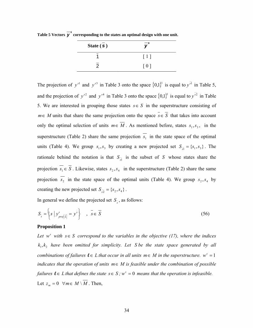
Table 5 Vectors s
y corresponding to the states an optimal design with one unit.
State ( s ) s
y
1 [ 1 ]
2 [ 0 ]
The projection of 1sy and 3sy in Table 3 onto the space 11,0 is equal to 1sy in Table 5,
and the projection of 2sy and 4sy in Table 3 onto the space 11,0 is equal to 2sy in Table
5. We are interested in grouping those states Ss in the superstructure consisting of
Mm units that share the same projection onto the space Ss that takes into account
only the optimal selection of units Mm . As mentioned before, states 31 , ss , in the
superstructure (Table 2) share the same projection 1s in the state space of the optimal
units (Table 4). We group 31, ss by creating a new projected set },{ 311ssS
s . The
rationale behind the notation is that 1s
S is the subset of S whose states share the
projection Ss 1 . Likewise, states 42 , ss in the superstructure (Table 2) share the same
projection 2s in the state space of the optimal units (Table 4). We group 42 , ss by
creating the new projected set },{ 422ssS
s .
In general we define the projected set s
S , as follows:
SsyysS ss
Lprojs
, (56)
Proposition 1
Let sw with Ss correspond to the variables in the objective (17), where the indices
21,kk have been omitted for simplicity. Let S be the state space generated by all
combinations of failures Ll that occur in all units Mm in the superstructure. 1sw
indicates that the operation of units Mm is feasible under the combination of possible
failures Ll that defines the state Ss ; 0sw means that the operation is infeasible.
Let MMmzm \ 0 . Then,

35
SsSswws
ss ,
This proposition implies that feasible operation of the integrated site depends only on the
failed/active status of the units selected from the superstructure. Therefore, all discrete
states that differ only on the failed/active status of the units not selected are identical in
terms of feasible or infeasible operation. The proof of this proposition can be found in
the appendix.
Proposition 2
The probability ( sprob ) of finding state Ss is equivalent to the summation over all the
probabilities ( sprob ) of finding the states s
Ss that share the same projection onto the
space S .
Ssprobprobs
Ss
ss
The proof of this proposition can be found in the appendix of this paper.
Proposition 3
Let *)(SFE be a Pareto-optimal solution found using the set S in equations (17)-(23),
(26)-(31), (39), (40), (46)-(57), and *
)(SFE be the Pareto-optimal solution found using
the reduced set S . Then, ** )()( SFESFE
This proposition is a consequence of Propositions 1 and 2; its proof can be found in the
appendix.
Proposition 3 proves the claim that solving the problem given by equations (17)-(23),
(26)-(31), (39), (40), (46)-(57) using the space state resulting from all the units postulated
in the superstructure, is equivalent to optimizing over the state space defined only for the
optimal selection of units.
Note that the propositions in this section can be easily extended to include the effect of
quadrature points ( 21 , kk ).
Example 1
The following example is based on a case study shown in previous work
concerned with evaluating (not optimizing) the E(SF) of a network of production
processes (Straub & Grossmann, 1990). The example of the chemical complex has been

36
modified to include intermediate storage. The objectives are to maximize the expected
stochastic flexibility E(SF) and to minimize the cost of installing parallel units,
intermediate storage, and increasing production capacity. The superstructure for the
integrated site is shown in Figure 10. This proposed integrated site has three potential
plants. Plant 1 transforms A to B and plant 2 transforms B to C. Plant 3 transforms A
directly into C. There are two potential parallel units for plant 1 (units 1I and 1II), one for
plant 2 (unit 2), and one for plant 3 (unit 3). All three plants have the potential addition of
storage.
Fig. 10 Integrated Site for the production of C from A.
Table 6 contains the data required to solve the problem using equations (17)-(23), (26)-
(31), (39), (40), (46)-(57). The base capacity provided in this table represents the
minimum capacity that each unit will have if it installed. This is a parameter considered
fixed in a previous design step. In an industrial setting this might correspond to a design
stage where continuous and discrete uncertainties are not considered. In Example 1, we
set the base capacities to the values given by Straub & Grossmann (1990). Note that the
Unit 1I
I2
I3
A C
I1
B
Unit 1II
Unit 2
Unit 3
Plant 1
Plant 2
Plant 3

37
fixed cost of installing a unit considers this base capacity, so that only additional capacity
has an extra variable cost.
There is only one total failure per unit in the integrated site, so that the number of failures
and number of units is equal. The uncertain parameters 1 and 2 are the supply of A and
demand of C. We discretize each of them using 5 collocation points. In order to test the
effect of the number of collocation points on the solution to the problem, we also solved
this example with 10 quadrature points and found that there is only a slight difference in
the optimal solution with a significant increase in solution time. Therefore, we only
report the results of using 5 collocation points. The sets 1,,,, KSNMJ and 2K used in
the formulation are described explicitly below:
}3,2,1{J ,
}3{ },2{ },1,1{ 321 MMM III ,
}3,2,1,1{ IIIM ,
}3{ },2{ },1{ },1{ 3211 LLLL IIIIII ,
}3,2,1,1{ IIIL ,
}16,...,2,1{S ,
}5,4,3,2,1{},5,4,3,2,1{ 21 KK ,
Table 6 Data for Example 1
Supply of A
[103 ton / day] Mean = 12 Std = 1
Demand of C
[103 ton / day] Mean = 7 Stand. Dev = 1
Probability of operation
Unit 1I
0.95
Unit 1II
0.95
Unit 2
0.92
Unit 3
0.87
Mass balance coefficient 1I = 0.92 1II = 0.92 2 = 0.85 3=0.75
Base capacity
[103 ton / day] 5 5 7 9
Mean time to repair [day] 0.25 0.25 0.25 0.25
Mean time to failure
[day] 4.75 4.75 2.88 1.67

38
Recall that each of the 16 states is described by a vector Lsy }1,0{ , where a 0 in the
thl position means that failure l is present when the integrated site is in state s . Table
7 describes each state in terms of its sy vector. For instance, state 1 corresponds to no
failure in the integrated site since Ly ll 11 .
Table 7 Discrete states for integrated site
sIy1
sIIy1 sy2 sy3 sprob
State 1 1 1 1 1 0.722
State 2 1 1 1 0 0.108
State 3 1 1 0 1 0.063
State 4 1 0 1 1 0.038
State 5 0 1 1 1 0.038
State 6 1 1 0 0 0.009
State 7 1 0 1 0 0.006
State 8 1 0 0 1 0.003
State 9 0 1 1 0 0.006
State 10 0 1 0 1 0.003
State 11 0 0 1 1 0.002
State 12 1 0 0 0 5e-4
State 13 0 1 0 0 5e-4
State 14 0 0 1 0 3e-4
State 15 0 0 0 1 1e-4
State 16 0 0 0 0 3e-5

39
We assume a normal distribution for both uncertain parameters, 1 (supply) and 2
(demand), and bound them at their mean value +/- four standard deviations. We then use
a five point Gaussian Quadrature scheme to obtain the quadrature points in Table 8,
which are derived from the roots of the Legendre polynomial (Carnahan et al., 1969).
Table 8 Five point Gaussian quadrature for demand and supply
Lower
Bound
1/ 21 kk
2/ 21 kk
3/ 21 kk 4/ 21 kk
5/ 21 kk
Upper
Bound
1 8.00 8.38 9.85 12.00 14.15 15.62 16.00
2 3.00 3.38 4.85 7.00 9.15 10.62 11.00
* - 0.237 0.479 0.569 0.479 0.237 -
* Quadrature weights
The value of the joint distribution can be evaluated at each point ( 21,kk ) and combined
with the quadrature weight for each point 2,1 kk , as shown below:
2
)()(exp
2
1
22
2222
21112211
212,1meankmeank
LULU
kkkk
(58)
Using the above formula we construct Table 9 with values of the joint distribution for all
discrete points.
Table 9 Probability of each discrete point (k1k2) according to joint distribution
1
11 k 21 k 21 k 41 k 51 k
12 k 2.5e-7 3.6e-5 4.3e-4 3.6e-5 2.5e-7
22 k 3.6e-5 5.0e-3 6.1e-2 5.0e-3 3.6e-5
32 k 4.3e-4 6.1e-2 7.3e-1 6.1e-2 4.3e-4
42 k 3.6e-5 5.e-3 6.1e-2 5.0e-3 3.6e-5
2
52 k 2.5e-7 3.6e-5 4.3e-4 3.6e-5 2.5e-7

40
Table 10 shows the cost function coefficients and the bounds for the decision variables.
Table 10 Cost coefficients and decision variable bounds for example 1
fixm
[MM USD]
10 UP1Icapacity
[103 tons/day]
7.5
varm
[MM USD]
1 UP1IIcapacity
[103 tons/day]
7.5
tank,nj
[MM USD]
1 UP2capacity
[103 tons/day]
10.5
UPv1
[103 tons]
1.23 UP3capacity
[103 tons/day]
13.5
UPv2
[103 tons]
1.75
UPv3
[103 tons]
2.25
Results
To validate our MILP formulation for maximizing E(SF), we fix the design to match the
one in the work by Straub and Grossmann (1990). In this design, all units are installed,
they have no intermediate storage, and they are not subject to extra capacity additions
(i.e. all units operate at their base capacity, as indicated in Table 1). The E(SF) reported
in their work is 0.8132, while the one obtained with the approach proposed in this paper
is 0.8066. Note that we are using five fixed quadrature points that might be inside or
outside the feasible region, while Straub and Grossmann (1990) collocate all five
quadrature points inside the feasible region, which involves solving a large NLP for the
evaluation of the E(SF). The small difference in the result can therefore be attributed to
the difference in the location of the collocation points.
The results that follow involve using the formulation described in this work with the data
presented in Tables 5 - 9 and Figure 10. To maximize the E(SF) and to minimize the cost
we determine the set of Pareto-optimal solutions by solving the proposed problem

41
repeatedly for different values of available capital investment. This is equivalent to
applying the -constrained method to the bi-criterion optimization problem. In this way,
the capital investment, cap, in equation (52) is limited by the available amount cap . The
results of maximum E(SF) for the different values of cap (Pareto-optimal solutions) are
summarized in Table 11 and Figure 11. Table 11 also indicates the computational time
required to find the optimal solution for each value of capital investment ( cap ). The
MILP model involves 404 discrete variables, 33,522 continuous variables, and 128,010
constraints. All results were obtained using the MILP solver CPLEX version 12.1,
running on GAMS 23.3. The results were obtained using a 2.8 GHz Intel Pentium 4
processor and 2.5 GB RAM. The optimality gap in CPLEX was set to 0.1%. We found
that this small gap reduced the computing time in about half for the instances that took
longer to solve.
Table 11 Value of optimal E(SF) and computational times for different levels of available capital
investment.
Capital
Investment
E(SF) CPU
seconds
Capital
Investment
E(SF) CPU
seconds
0 0 2 35 0.964 602
10 0.062 9 40 0.967 150
11 0.818 12 45 0.983 144
15 0.869 9 50 0.987 6
20 0.870 143 55 0.988 4
25 0.870 143 60 0.988 2
30 0.870 257
As can be seen in Figure 11, the set of Pareto-optimal solutions is nonconvex and the
E(SF) values increase step-wise rather than smoothly as the available capital increases.
This effect is the result of having discrete probabilities for states s and weights for the
collocation points ( 21,kk ). The state probability is sprob and the collocation point weight
is 2,1 kk in equation (17).

42
0.0
0.1
0.2
0.3
0.4
0.5
0.6
0.7
0.8
0.9
1.0
0 10 20 30 40 50 60Capital Investment [MM USD]
E(S
F)
Fig. 11 Pareto curve of maximal E(SF) and minimum cost for Example 1
Table 12 presents the details of the optimal design for some values of available capital
investment. Namely, the designs for 25, 35 and 45 units of available capital investment
are described in this table. The capacities indicated there are calculated as base capacity
(problem parameter) plus capacity addition (decision variable). This table shows the
values of the linear approximation of the standard deviation of the inventory level
(equation (46)), as well as the exact standard deviation calculated from equation (44).
The average overestimation of standard deviation of inventory levels for the complete set
of Pareto-optimal solutions presented in Table 11 is 75%. The overestimation effect can
be somewhat corrected by the truncation parameters up and lo in equations (47) and
(48). In this example we set those parameters equal to four.
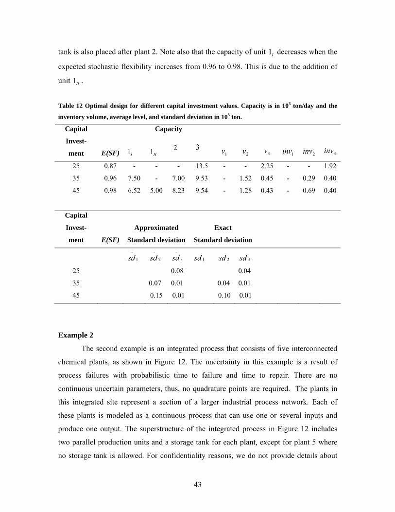
In the solutions described in Table 12, storage tanks are placed after plants that directly
feed the end consumer, so that the effect of any upstream failure is buffered by these
storage tanks. In the low capital investment solutions, the storage tank is placed after
plant 3, which is the most unreliable. When more capital becomes available a storage
43
tank is also placed after plant 2. Note also that the capacity of unit I1 decreases when the
expected stochastic flexibility increases from 0.96 to 0.98. This is due to the addition of
unit II1 .
Table 12 Optimal design for different capital investment values. Capacity is in 103 ton/day and the
inventory volume, average level, and standard deviation in 103 ton.
Capacity Capital
Invest-
ment E(SF) I1 II1 2 3 1v 2v 3v
1inv 2inv 3inv
25 0.87 - - - 13.5 - - 2.25 - - 1.92
35 0.96 7.50 - 7.00 9.53 - 1.52 0.45 - 0.29 0.40
45 0.98 6.52 5.00 8.23 9.54 - 1.28 0.43 - 0.69 0.40
Capital
Invest-
ment E(SF)
Approximated
Standard deviation
Exact
Standard deviation
1
~
sd 2
~
sd 3
~
sd 1sd 2sd 3sd
25 0.08 0.04
35 0.07 0.01 0.04 0.01
45 0.15 0.01 0.10 0.01
Example 2
The second example is an integrated process that consists of five interconnected
chemical plants, as shown in Figure 12. The uncertainty in this example is a result of
process failures with probabilistic time to failure and time to repair. There are no
continuous uncertain parameters, thus, no quadrature points are required. The plants in
this integrated site represent a section of a larger industrial process network. Each of
these plants is modeled as a continuous process that can use one or several inputs and
produce one output. The superstructure of the integrated process in Figure 12 includes
two parallel production units and a storage tank for each plant, except for plant 5 where
no storage tank is allowed. For confidentiality reasons, we do not provide details about

44
the processes or the chemicals involved in the integrated site. Also, the capital investment
values of the Pareto-optimal solutions in Figure 13 do not represent the real costs. Table
13 shows the constant rate of supply of raw materials and the constant rate of
consumption of finished products. The base processing capacity and the mass balance
(yield) coefficient of the units in each plant is shown in Table 14. In this example, the
base processing capacities correspond to those required to satisfy the demand of products
1 and 5 when no failures occur. The mass coefficient that corresponds to m in equation
(20) is calculated as the ratio of output over inputs. Notice that some of these coefficients
are larger than one, implying that several mass units of output are produced for each mass
unit of inputs. The increase in mass flow is a result of adding fillers, solvents, etc. to the
product flows of each plant. We do not model directly these secondary flows but include
them indirectly through the mass balance coefficients in Table 14. Likewise, waste
streams not included explicitly in the process network of Figure 12 are indirectly
modeled by mass balance coefficients smaller than one. The plants in the integrated site
consume raw materials provided by external suppliers as well as intermediate products
from other plants. Different inputs must be fed according to the stoichiometric
coefficients given in Table 15. For instance, Plant 2 (second row in Table 15) requires 1.3
mass units of product 1 per unit of raw material 2.
Fig. 12 Industrial integrated process
Plant 1
Plant 2
Plant 4
Plant 3 Plant 5
RawMaterial2
Product 1
Product 5RawMaterial1
RawMaterial3
RawMaterial4
RawMaterial5

45
Table 13 Supply and Demand data in industrial case study
1 2 3 4 5 Supply of Raw Material
[ ton / h] 20 45 21 12 42
1 5 Demand of Product
[ ton / h] 32.5 50
Table 14 Base processing capacity and mass balance coefficients in industrial case study
Production
Units in
Plant 1
Production
Units in
Plant 2
Production
Units in
Plant 3
Production
Units in
Plant 4
Production
Units in
Plant 5
Mass
balance
coefficient
5.29 0.69 0.70 3.87 0.46
Base
capacity
[ ton / h]
13.9 73.4 53.7 8.3 109.6
Table 15 Mass balance coefficients for the feed of external raw materials (RM) and intermediate
products (P) for each plant.
RM1 RM2 RM3 RM4 RM5 P1 P2 P3 P4 P5
Plant 1 1 0 0 0 0 - 0 0 0 0
Plant 2 0 1 0 0 0 1.3 - 0 0 0
Plant 3 0 0 1 0 0 0 17.5 - 0 0
Plant 4 0 0 0 1 0 0 0 0 - 0
Plant 5 0 0 0.4 0 1 0 0 1.3 1.1 -

46
The times to failure TTF of all the units in the system are modeled using an exponential
distribution, while the times to repair TTR correspond to a normal distribution. We have
indicated that the Markov chain modeling technique requires exponential distributions for
the TTF and TTR in order to accurately represent the transient behavior of the system.
However, it is possible to obtain useful results for the stationary (long term) behavior of
the system even when the TTR is represented by a normal distribution. In this case, we
only need to know the mean time to repair ( MTTR ) and use it as the mean of an
exponential distribution (Billinton and Allan, 1992).
The network in Figure 12 is subjected to different types of partial and total random
failures. For instance, each of the two production units in plant 2 is subject to six different
types of total failures (e.g. different equipment in the unit force the production to stop),
three types of partial failures that cause a 25% rate reduction, and two partial failures that
cause a 10% rate reduction, resulting in 12 discrete states (11 failures plus the “no
failure” state). Applying the discrete state modeling approach discussed so far in this
paper results in 144 states just for the units in this plant. The total number of system
states obtained from the possible combinations of discrete states of each of the units of all
the plants is of the order of 1010x5 . To reduce this number, the failures with the same
related rate reduction that occur in the same plant can be aggregated as one equivalent
failure. For instance, the six different total failures in plant 2 can be modeled as one
equivalent failure. Using this technique the original state space is rigorously reduced to
an equivalent one with 410x8 discrete states. The fact that this is still a state space with
large dimensionality emphasizes the need for future work on complexity reduction
techniques based on decomposition and bounding search procedures.
In this work, to further reduce the number of states, we limit the problem to considering
the 157 most probable states since these cover approximately 99% of the long term
operating horizon. The MILP problem with the 157 states consists of 162 binary
variables, 184,372 continuous variables, and 504,511 constraints. All results were
obtained using the MILP solver CPLEX version 12.1, running on GAMS 23.3, with a 2.8
GHz Intel Pentium 4 processor and 2.5 GB RAM. A 2 percent gap between lower and
upper bounds in the branch and bound algorithm was used as termination criteria for
CPLEX.

47
Figure 13 shows the Pareto curve of maximum E(SF) and minimum capital cost. Table
16 contains the cost coefficients used to generate this curve and the bounds on the
decision variables. Table 17 shows the CPU time required to obtain each point in the
curve of Figure 13, and Table 18 gives details of the optimal designs corresponding to
some capital investment levels.
0.0
0.1
0.2
0.3
0.4
0.5
0.6
0.7
0.8
0.9
1.0
400 500 600 700 800 900 1000
Capital Investment [MM USD]
E(S
F)
Fig. 13 Pareto curve of maximal E(SF) and minimum cost for Example 2

48
Table 16 Cost coefficients and decision variable bounds for Example 2
fixm
[MM USD]
100 UP/11 III
capacity
[ton/h]
20.9
varm
[MM USD]
10 UP/22 III
capacity
[ton/h]
110.4
nj ,
[MM USD]
0.005 UP/33 III
capacity
[ton/h]
80.7
UPv1
[103 ton]
15,000 UP/44 III
capacity
[ton/h]
12.3
UPv2
[103 ton]
7,500 UP/55 III
capacity
[ton/h]
164.6
UPv3
[103 ton]
7,500
UPv4
[103 ton]
5,000
UPv5
[103 ton]
0
Table 17 CPU time required to obtain a solution for different capital investments.
Capital
Investment
CPU
seconds
Capital
Investment
CPU
seconds
400 <1 750 844
500 6 800 294
550 35 850 709
600 202 900 338
650 850 950 156
700 186 1000 111

49
Table 18 Optimal design for different capital investment values for Example 2.
Capacity Capital
Investment
E(SF)
I1 II1 I2 II2 I3 II3
500 0.74 13.9 - 73.4 - 53.7 -
600 0.83 13.9 - 73.4 73.4 53.7 -
850 0.94 13.9 - 73.4 73.4 53.7 53.7
1000 0.98 13.9 13.9 73.4 73.4 53.7 53.7
Capacity
I4 II4 I5 II5
500 8.3 - 109.6 -
600 8.3 - 109.6 -
850 8.3 - 109.6 114.6
1000 10.5 - 109.6 109.6
v1 v2 v3 v4 v5
500 - - - - -
600 - - - - -
850 - - - - -
1000 - 423.1 909.0 227.3 -
inv1 inv2 inv3 inv4 inv5
500 - - - - -
600 - - - - -
850 - - - - -
1000 - 211.6 454.5 170.5 -
Notice that all plants are required as part of the integrated process, and therefore a
minimum investment of 500 MM USD is required. Note that this amount represents the
fixed cost of installing one unit for each plant, at the given base capacity (Table 14). The

50
500 MM USD design is able to provide the required products to external consumers when
all plants are running. However, when random failures are introduced the integrated site
is only able to deliver the required amounts of products 74% of the time. The addition of
one parallel production unit (600 MM USD design in Table 18) increases the expected
stochastic flexibility to 0.83. When multiple parallel units are installed together with
intermediate storage tanks the fraction of time of feasible operation (or E(SF)) can be
increased to 0.94 (850 MM USD design in Table 18), or even to 0.98 (1000 MM USD
design in Table 18).
Conclusions
In this paper, we have proposed an MILP bi-criterion formulation for optimizing the
design of an integrated site subject to random failures and random supply and demand.
The two optimization criteria are the maximization of the expected stochastic flexibility
E(SF) and the minimization of the capital investment. The proposed formulation has
several novel features that constitute the main contributions of this work. Namely, it
captures the effect of random events on the levels of material in intermediate storage, and
it integrates the idea of superstructure optimization in a production network with the
concept of discrete states in a continuous time Markov chain. We used this formulation to
solve the optimal design problem in two small networks; one adapted from the existing
literature and the other provided by a major chemical company. We identified the need to
address the exponential growth in problem size with the number of discrete states as a
result of an increase in number of production units or failure modes per unit. In future
work we will develop algorithmic techniques to deal with the growth in problem size.
Also, the systematic reduction of the number of discretization points for continuous
uncertain parameters, as in Novak and Kravanja (2008), represents a potential line of
future work. Finally, we will incorporate realistic cost functions in order to provide
meaningful solutions to industrial problems.
Acknowledgement
The authors acknowledge Naoko Akiya and Jee Park from The Dow Chemical Company
for their help during the development of the formulation presented in this paper. The
authors also acknowledge The Dow Chemical Company for providing financial support
for this work.

51
References
Bansal V., D. P. Perkins and E. N. Pistikopoulos, (2000). Flexibility analysis and design of linear systems by parametric programming. AIChE Journal, 46(2) 335 – 354.
Bansal V., D. P. Perkins and E. N. Pistikopoulos, (2002). Flexibility analysis and design
using a parametric programming framework. AIChE Journal, 48(12) 2851 – 2868. Billinton R. and R. N. Allan, Reliability Evaluation of Engineering Systems. Plenum
Press, New York (1992). Carnahan B., H. A. Luther and J. O. Wilkes, Applied Numerical Methods. Wiley, New
York (1969). Cheng L., E. Subrahmanian and A. W. Westerberg, (2003). Design and planning under
uncertainty: issues on problem formulation and solution. Computers and Chemical Engineering, 27, 781 – 801.
Davies K. M. and C. L. E. Swartz, (2008). MILP Formulations for Optimal Steady-State
Buffer Level and Flexible Maintenance Scheduling. MASc Thesis, McMaster University.
Ehrgott M, Multicriteria Optimization. Springer Berlin, Heidelberg (2005). Feord D., C. Jakeman and N. Shah, (2002). Modelling Multi-site Production to Optimise
Customer Orders. 12th European Symposium on Computer Aided Process Engineering – ESCAPE 12, A. Povoa and H. Matos (Editors).
Goel H. D., J. Grievink and M. P. C. Weijnen, (2003). Integrated optimal reliable design,
production and maintenance planning for multipurpose process plants. Computers and Chemical Engineering, 27, 1543 – 1555.
Henley E.J. and H. Hoshino, (1977). Effect of Storage Tanks on Plant Availability.
Industrial and Engineering Chemistry Fundamentals, 16(4), 439 – 443. Heyman D. P. and M. J. Sobel, Stochastic Models in Operations Research, Volume
I.McGraw-Hill, New York (1982). Hooker J. N., H. Yan, I. E. Grossmann and R. Raman, (1994). Logic cuts for processing
networks with fixed charges. Computers and Operations Research, 21(3), 265 – 279. Kimm N. K., (2008). Economic and Environmental Aspects of Integration in Chemical
Production Sites. PhD Thesis, Universität Karlsruhe. Novak Pintaric Z. and Z. Kravanja (2008). Identification of critical points for the design
and synthesis of flexible processes. Computers and Chemical Engineering, 32, 1603 – 1624.

52
Orban-Mihalyko E. and B. G. Lakatos, (2004). Intermediate storage in batch/continuous
processing systems under stochastic operation conditions. Computers and Chemical Engineering, 28, 2493 – 2508.
Pistikopoulos E. N., T. V. Thomaidis, A. Melin, and M.G. Ierapetritou (1996).
Flexibility, reliability and maintenance considerations in batch plant design under uncertainty. Computers and Chemical Engineering, 20, S1209 – S1214.
Pistikopoulos E. N., C. G. Vassiliados, J. Arvela and L.G. Papageorgiou, (2001).
Interaction of maintenance and production planning for multipurpose process plants – a system effectiveness approach. Industrial and Engineering Chemistry Research, 40, 3195 – 3207.
Sherali H. D., J. Desai and T. S. Glickman, (2008). Optimal Allocation of Risk-
Reduction Resources in Event Trees. Mangement Science, 54(7), 1313 – 1321. Straub D. A. and I. E. Grossmann, (1990). Integrated stochastic metric of flexibility for
systems with discrete state and continuous parameter uncertainties. Computers and Chemical Engineering, 14(9), 967 – 985.
Straub D. A. and I. E. Grossmann, (1993). Design Optimization of Stochastic Flexibility.
Computers and Chemical Engineering, 17(4), 339 – 354. Uspensky J. V., Introduction to mathematical probability. McGraw-Hill Book Company,
New York (1937). Wassick, J. M. Enterprise-wide optimization in an integrated chemical complex.
Computers and Chemical Engineering (2009), doi:10.1016/j.compchemeng.2009.06.002

53
Appendix
Proof of Proposition 1
Remark Recall that },1:{ MmzmM m refers to the set of units in the optimal
flowsheet. Also, recall that the set Mm
mLL
refers to the failure modes of the units in
the optimal flowsheet, and that S is the state space derived from all the combinations of
simultaneous failures in L .
The optimization problem can be express in a general form as:
Dd
w
SswMu
Ssuydzpsfflowg
Ssydzpsfflowh
ts
wprob
S
ss
sssssss
ssssss
Ss
ss
||}1,0{
)1(
),,,,,,(
0),,,,,,(
..
max
where d are all the design variables other than z , and D is a feasible set defined by the
bound constraints on the design variables.
For a given parameter sy , a design zd , and a pair ssps , we can solve )(h for
ss fflow , . Therefore, we can express the optimization problem equivalently as:
Dd
w
SswMu
Ssuydzpsr
ts
wprob
S
ss
sssss
Ss
ss
||}1,0{
)1(
),,,,(
..
max
(A.1)
Let us solve the problem A.1 using the state-space S derived from all the units in the
superstructure and rewrite it considering only the units selected in the optimal flowsheet

54
(i.e. those units m such that 1mz ). The corresponding state-space for this flowsheet is
S
Dd
w
SswMu
Ssuydpsr
ts
wprob
S
ss
sssss
Ss
ss
||}1,0{
)1(
),,,(
..
max
(A.2)
We now proceed to show that the feasible regions of the variables ,,ps and d are the
same in problems (A.1) and (A.2).
Equations (56) and (57) enforce the condition that the feasible regions of s
s Ss in
(A.1) and Sss in (A.2) are the same. The feasible region of d is the same in
(A.1) and (A.2) since the constraints that define D (in Dd ) are independent of the
state-space.
The feasible region for s
s Sspc in (A.1) is given by non-negativity and equations
(31) and (53). For the components s
sm SsMMmpc ,\ in (A.1) equations (53) is
dominant since MMmzm \0 . For the components s
sm SsMmpc , in (A.1)
equation (53) is redundant and the feasible region is given by non-negativity and equation
(31).
In problem A.2 the feasible region of MmSsps sm
, is given by non-negativity
and equation (31).
Since by definition the projection of sy onto the state-space S is exactly sy , equation
(31) is identical for all s
SsMm , in (A.1) and for all SsMm , in (A.2). We
already established that s
sm SsMMm pc ,\0 so that the units MMm \ can be
treated as non-existent in (A.1). These last two statements imply that the feasible region
of s
s Sspc in (A.1) is the same as Sspc s in (A.2).
55
Given the results obtained for the feasible regions of the variables ,,ps and d in (A.1)
and (A.2), the functions s
s Ssr )( in (A.1) and Ssr s )( in (A.2) have the same
feasible range. It then follows that the optimal solution s
s Ssw , of (A.1) and
Ssws of (A.2) are identical.
Thus, SsSswws
ss , , as defined in Proposition 1 is true. �
Proof of Proposition 2
From equation (33)
Ssppprob
LyLy
s
ss
,)1(
,1:,0: ll
l
ll
l
ll
(A.3),
and
SLyLy
ls Ssppprob
ss
,)1( ,1:,0: ll
lll ll
. (A.4)
We can split the set L in the multiplication of equation (A.4) into L and LL \ so that
S
LLyLLyLyLy
s Ssppppprobssss
,)1( )1( \,1:\,0:,1:,0: ll
lll
lll
lll
l
llll
. (A.5)
Recall that the projection of Lsy 1,0 onto sLs yy 1,0 , SsSss
, . We can use
this expression and substitute the multiplication over Lys ll : in (A.5) for a
multiplication over Lys ll : , so:
SsSsppppprobs
LLyLLyLyLy
s
ssss
, ,)1( )1(
\,1:\,0:,1:,0: ll
l
ll
l
ll
l
ll
l
llll
, (A.6)
and by equation (A.3):
SsSsppprobprobS
LLyLLy
ss
ss
, ,)1( \,1:\,0: ll
lll
l
ll
(A.7)
Summing over S
S s ,
Ssppprobprobs
sss
Ss LLyLLy
s
Ss
s
,)1( \,1:\,0: ll
lll
l
ll
(A.8)
On the other hand, using the conditional probability notation and equation (A.7):

56
SsSsprobppprobprobprobs
s
LLyLLy
sss
ss
, , |)1( )|(\,1:\,0: ll
lll
l
ll
(A.9)
The conditional probability notation (A|B), which is read “A given B”, in equation (A.9)
implies that:
SsSsppprobprobs
LLyLLy
ss
ss
, , )1( )|(\,1:\,0: ll
lll
l
ll
(A.10)
By its definition the collection of statess
S covers all the possible combinations of
failures LLl \ , and hence
Ssprobprob s
Ss
s
S
1 )( (A.11)
Using equation (A.10) in (A.11),
1 )1( \,1:\,0:
S
ssSs LLyLLy
ppll
lll
l
ll
(A.12)
Substituting equation (A.12) in equation (A.8) completes the proof. �
Proof of proposition 3
*)*( s
Ss
swprobSFE
and **)( s
Ss
swprobSFE
, where ws* is the value of ws in the
optimal solution.
The set S can be constructed as Ss
sSS
. It then follows that
Ss sSs
sswprobSFE *)*( (A.13)
By Proposition 1 SsSswws
ss , ** .
Hence,
Ss Ss
ss
s
probwSFE *)*( , and by Proposition 2,
*)(*)*( SFEprobwSFE
Ss
ss
and the proof is complete. �