optimal design of natural and hybrid laminar flow …optimal design of natural and hybrid laminar...
TRANSCRIPT

Optimal Design ofNatural and Hybrid Laminar Flow Control
on Wingsby
Jan Pralits
October 2003Technical Reports from
Royal Institute of TechnologyDepartment of Mechanics
SE-100 44 Stockholm, Sweden

Typsatt i AMS-LATEX.
Akademisk avhandling som med tillstand av Kungliga Tekniska Hogskolan iStockholm framlagges till o!entlig granskning for avlaggande av teknologiedoktorsexamen onsdagen den 7:e oktober 2003 kl. 10.15 i Kollegiesalen, Admin-istrationsbyggnaden, Kungliga Tekniska Hogskolan, Valhallavagen 79, Stock-holm.
c!Jan Pralits 2003
Universitetsservice, Stockholm 2003

Optimal design of natural and hybrid laminar flow control on wings.Jan PralitsDepartment of Mechanics, Royal Institute of TechnologySE-100 44 Stockholm, Sweden.
AbstractMethods for optimal design of di!erent means of control are developed in thisthesis. The main purpose is to maintain the laminar flow on wings at a chordReynolds number beyond what is usually transitional or turbulent. Linear sta-bility analysis is used to compute the exponential amplification of infinitesimaldisturbances, which can be used to predict the location of laminar-turbulenttransition. The controls are computed using gradient-based optimization tech-niques where the aim is to minimize an objective function based upon, or re-lated to, the disturbance growth. The gradients of the objective functions withrespect to the controls are evaluated from the solutions of adjoint equations.
Sensitivity analysis using the gradients of the disturbance kinetic energywith respect to di!erent periodic forcing show where and by what means controlis most e"ciently made. The results are presented for flat plate boundary layerflows with di!erent free stream Mach numbers.
A method to compute optimal steady suction distributions to minimize thedisturbance kinetic energy is presented for both incompressible and compress-ible boundary layer flows. It is shown how to formulate an objective function inorder to minimize simultaneously di!erent types of disturbances which mightexist in two, and three-dimensional boundary layer flows. The problem for-mulation also includes control by means of realistic pressure chambers, andresults are presented where the method is applied on a swept wing designed forcommercial aircraft.
Optimal temperature distributions for disturbance control are presentedfor flat plate boundary layer flows. It is shown that the e"ciency of the controldepends both on the free stream Mach number, and whether the wall down-stream of the control domain is insulated, or heat transfer occurs.
Shape optimization is presented with the aim of reducing the aerodynamicdrag, while maintaining operational properties. Results of optimized airfoilsare presented for cases where both the disturbance kinetic energy, and wavedrag are reduced simultaneously while lift, and pitch-moment coe"cients aswell as the volume are kept at desired values.
Descriptors: fluid mechanics, laminar-turbulent transition, boundary layer,laminar flow control, natural laminar flow, adjoint equations, optimal control,objective function, PSE, APSE, ABLE, HLFC, eN -method, Euler equations

Preface
The thesis is based on and contains the following papers:
Paper 1. Pralits, J. O., Airiau, C., Hanifi, A. & Henningson, D. S.2000 Sensitivity analysis using adjoint parabolized stability equations for com-pressible flows. Flow, Turbulence and Combustion, 65(3), 312–346
Paper 2. Pralits, J. O., Hanifi, A. & Henningson, D. S. 2002 Adjoint-based optimization of steady suction for disturbance control in incompressibleflows. Journal of Fluid Mechanics, 467, 129–161
Paper 3. Pralits, J. O. & Hanifi, A. 2003 Optimization of steady suc-tion for disturbance control on infinite swept wings. Physics of Fluids, 15(9),2756–2772
Paper 4. Pralits, J. O. & Hanifi, A. 2003 Optimization of steady walltemperature for disturbance Control. To be submitted.
Paper 5. Amoignon, O., Pralits, J. O., Hanifi, A., Berggren, M. &Henningson, D. S. 2003 Shape optimization for delay of laminar-turbulenttransition. Technical Report FOI-R–0919–SE, at the Swedish Defence ResearchAgency, FOI, Aeronautics Division, FFA.
The papers are re-set in the present thesis format.
iv
PREFACE v
Reports and proceedings related to the content of the thesis
Pralits, J. O., Hanifi, A. & Henningson, D. S. 2000 Adjoint-based Suc-tion Optimization for 3D Boundary Layer Flows. Technical Report FFA TN2000-58, at the Swedish Defence Research Agency, FOI, Aeronautics Division,FFA.
Airiau C., Pralits, J. O., Bottaro, A. & Hanifi, A. 2001 Adjoint PSEand boundary layer equations for HLFC. Technical Report TR 10, ALTTA De-liverable No D3.1.4-1 .
Hanifi, A., Pralits, J. O., Zuccher, S, Donelli, R. & Airiau, C. 2001Adjoint-based Sensitivity Analysis: Validation and Comparison. Technical Re-port TR 22, ALTTA Deliverable No D3.1.4-2 .
Pralits, J. O., Hanifi, A. & Mughal, S. 2002 Optimal suction design forHLFC applications. Technical Report TR 57, ALTTA Deliverable No D3.1.4-6 .
Pralits, J. O.& Hanifi, A. 2002 Optimization of Steady Suction for Distur-bance Control on Infinite Swept Wings. In proceeding no. FEDSM2002-31055at ASME Fluids Engineering Division Summer Meeting, Montreal, Canada.
Pralits, J. O.& Hanifi, A. 2003 Optimal Suction Design for HLFC Appli-cations. AIAA paper 2003-4164, 33rd AIAA Fluid Dynamics Conference andExhibit, Orlando, Florida.


Contents
Preface iv
Part 1. Summary 1
Chapter 1. Introduction 3
Chapter 2. Modeling the flow 52.1. Governing equations 52.2. The steady boundary layer flow 62.3. Linear stability equations 72.4. Parabolized stability equations 8
2.4.1. Assumption and derivation 92.4.2. Step-size restriction 102.4.3. Comparison with DNS 11
Chapter 3. Transition prediction 13
Chapter 4. Disturbance control 174.1. Suction/blowing 184.2. Wall cooling 194.3. Wall-shaping 20
4.3.1. Pressure gradient 204.3.2. Curvature 21
Chapter 5. Optimal design for disturbance control 235.1. Background 23
5.1.1. Natural laminar flow 245.1.2. Laminar flow control 245.1.3. Control by blowing and suction 25
5.2. Gradient evaluation using adjoint equations 265.3. Outline of the current approach 28
5.3.1. Objective function 28
vii

viii CONTENTS
5.3.2. Optimal design cases 295.4. Optimal laminar flow control 31
5.4.1. Sensitivity analysis using periodic forcing 315.4.2. Wave cancellation 345.4.3. Hybrid laminar flow control 36
5.5. Shape optimization for natural laminar flow 435.5.1. Problem formulation and gradients 435.5.2. Mesh displacements, parametrization and
geometrical constraints 445.5.3. Solution procedure 455.5.4. An optimal design case 46
Chapter 6. Summary & conclusions 49
Acknowledgment 51
Bibliography 52
Part 2. Papers 57
Paper 1. Sensitivity analysis using adjoint parabolizedstability equations for compressible flows 61
Paper 2. Adjoint-based optimization of steady suctionfor disturbance control in incompressible flows 89
Paper 3. Optimization of steady suction fordisturbance control on infinite swept wings 129
Paper 4. Optimization of steady wall temperaturefor disturbance control 167
Paper 5. Shape optimization for delay oflaminar-turbulent transition 197

Part 1
Summary


CHAPTER 1
Introduction
The final design of an aircraft wing is always a compromise in the intersectionof feasibility imposed by various requirements. Aerodynamics is one importantaspect as it enables calculations of operational properties such as lift, momentsand drag. Traditionally, the design work has been an iterative process betweentheory and experiments, in which the latter has often been costly. Orville andWilbur Wright1 spend many hours in the laboratory using their home madewind tunnel to test di!erent types of wings in order to increase the lift coef-ficient enough enabling their first controlled flight in 1903. Nowadays, whenavailable computer power increases rapidly and numerical tools increase in ac-curacy and modeling capability, both experiments and numerical calculationsare part of the total design process. For a computational method to be reli-able as a tool, it must be based on a mathematical model which provides anappropriate representation of the significant features of the flow, such as shockwaves, boundary layers and laminar-turbulent transition.
The total drag of an aircraft is mainly given by the sum of pressure or wavedrag, related to the existence of shock waves for transonic and supersonic flows,and viscous drag, whose magnitude depends on whether the flow is laminar orturbulent. Turbulent flow, in some cases, produces a much larger drag; thusimportant research e!orts have been devoted to find e"cient means to keep theflow laminar over the largest possible portion of the wing surface. A similarsituation is encountered in other industrial applications (wind-turbine blades,di!user inlets), where less turbulence means less energy spent to achieve thesame motion, which in turn translates directly to less pollution and reducedexpenses.
Control of fluid flow can be made by means of active or passive controldevices. A natural passive device is the shape of the wing itself, and reduction ofdrag is obtained by a properly made design. An approach in which the aim is toincrease the laminar portion of the wing is usually called Natural Laminar Flow(NLF) design. Other examples are found looking at the surface structure whereroughness elements or cavities, such as on golf-balls, are sometimes used. Anactive device which has been investigated extensively is suction of air throughthe whole or parts of the wing which have been equipped with a porous surface.This technique falls into the category of Laminar Flow Control (LFC) which
1The 17th of December 2003 is the 100 year anniversary of the first controlled flight performedby O. and W. Wright in 1903 which had a duration of 59 seconds.
3
4 1. INTRODUCTION
means to maintain the laminar flow at a chord Reynolds number beyond whatis usually transitional or turbulent when no control is used. With this definitionit does not cover cases where the aim is to relaminarize already turbulent flow.A combination of NLF and LFC in which the active control is imposed only ona part of the wing is usually called Hybrid Laminar Flow Control (HLFC). Adistinctive feature of any flow design process as opposed to one not involvingfluids is that the computation is often very costly, or even totally out of reach ofany existing computer when turbulent flow in complex geometries is involved.It is therefore common practice to introduce approximations. Once a reliableand e"cient numerical tool is available, a straight-forward approach for designof passive or active devices is a vast parameter study in order to find thecontrol which best meets certain criteria set on the operational properties, anddecreases the drag. In most cases the number of possible designs is large, andit is very unlikely that a truly optimal design can be found without assistanceof automatic tools. For this reason, there is a growing interest in utilizingnumerical optimization techniques to assist in the aerodynamic design process.
The aim of the work presented in this thesis is to integrate physical model-ing of the flow and modern optimization techniques in order to perform optimalNLF and HLFC design. Gradient-based optimization techniques are used andthe gradients of interest are derived using adjoint equations. When one consid-ers highly streamlined bodies such as wings, there is often a substantial laminarportion, thus a correct transition prediction becomes essential for a good es-timate of the total drag. The governing equations for the physical problemare introduced in chapter 2, and transition prediction is covered in chapter 3.Means of control laminar-turbulent transition is discussed in 4, and the ap-proach taken here to perform optimal HLFC and NLF is given in chapter 5.A summary and conclusions are given in chapter 6, and papers related to thework presented in these chapters are given in the second part.

CHAPTER 2
Modeling the flow
2.1. Governing equationsThe motion of a compressible gas is given by the conservation equations ofmass, momentum and energy and the equation of state. The conservationequations in dimensionless form and vector notation are
!"
!t+" · ("u) = 0, (2.1)
"!!u!t
+ (u ·")u"
= #"p +1Re"!#(" · u)
"+
1Re" ·!µ("u +"uT)
", (2.2)
"cp
!!T
!t+(u·")T
"=
1Re Pr
"·($"T )+(%#1)M2!!p
!t+(u·")p+
1Re
#", (2.3)
%M2p = "T, (2.4)with viscous dissipation given as
# = #(" · u)2 +12µ!"u +"uT
"2.
Here t represents time, ", p, T stand for density, pressure and temperature, uis the velocity vector. The quantities #, µ stand for the second and dynamicviscosity coe"cients, % is the ratio of specific heats, $ the heat conductivityand cp the specific heat at constant pressure. All flow quantities are madedimensionless by corresponding reference flow quantities at a fixed streamwiseposition x!
0, except the pressure which is made dimensionless with two timesthe corresponding dynamic pressure. The reference length scale is fixed andtaken as
l!0 =
#&!0x!
0
U!0
.
The Mach number, M , Prandtl number, Pr and Reynolds number, Re aredefined as
M =U!
0$$%T !
0
, Pr =µ!
0c!p0
$!0
, Re =U!
0 l!0&!0
,
where $ is the specific heat constant and superscript ! refers to dimensionalquantities. In order to generalize the equations for geometries with curvedsurfaces an orthogonal curvilinear coordinate system is introduced. The trans-formation from Cartesian coordinates X i to curvilinear coordinates xi is made
5

6 2. MODELING THE FLOW
using the scale factors hi. The definition of the scale factors and correspondingderivatives mij are given as
h2i =
3%
j=1
&!Xj
!xi
'2and mij =
1hihj
!hi
!xj.
Using the scale factors, an arc length in this coordinate system can be writtenas
ds2 =3%
i=1
&hidxi
'2.
Here, x1, x2 and x3 are the coordinates of the streamwise, spanwise and wallnormal directions respectively1.
2.2. The steady boundary layer flowIn this thesis flat plate boundary-layer flows with and without pressure gradientare considered as well as the flow past a swept wing with infinite span. All thesedi!erent flows are special cases of the flow past a swept wing with infinite span.They are here given in dimensionless primitive variable form as
1h1
!("U)!x1
+!("W )!x3
= 0, (2.5)
"U
h1
!U
!x1+ "W
!U
!x3= # 1
h1
dPe
dx1+
1Re
!
!x3
&µ!U
!x3
', (2.6)
"U
h1
!V
!x1+ "W
!V
!x3=
1Re
!
!x3
&µ!V
!x3
', (2.7)
cp"U
h1
!T
!x1+ cp"W
!T
!x3=
1RePr
!
!x3
&$!T
!x3
'
+ (% # 1)M2( U
h1
dPe
dx1+
µ
Re
!& !U
!x3
'2+& !V
!x3
'2"), (2.8)
where U, V, W are the streamwise, spanwise and wall-normal velocity compo-nents, respectively2. Under the boundary-layer assumptions, the pressure isconstant in the direction normal to the wall, i. e. P = Pe(x1). The equation ofstate can then be expressed as
%M2Pe = "T,
and the streamwise derivative of the pressure is given by the inviscid flow as
dPe
dx1= #"eUe
dUe
dx1.
1In the second paper the coordinates are given as x1 = x, x2 = z and x3 = y, where x, y, zare the streamwise, wall normal and spanwise coordinates, respectively.2In the second paper U, V, W are the streamwise, wall normal and spanwise velocity compo-nents respectively.
2.3. LINEAR STABILITY EQUATIONS 7
The corresponding boundary conditions with no-slip conditions and assumingan adiabatic wall condition are
U = V = W =!T
!x3= 0, at x3 = 0,
(U, V, T )% (Ue, Ve, Te), as x3 % +&.
The variables with subscript e are evaluated at the boundary layer edge and arecalculated from well known fundamental relations using respective free streamvalues found either from measurements or inviscid flow calculations. The firstrelation is that the total enthalpy is constant along a streamline in an inviscid,steady, and adiabatic flow. The second is the isentropic relations which are usedto obtain the relation between pressure, density and temperature expressed asratios between total and static quantities.
2.3. Linear stability equationsIn order to derive the linear stability equations, we decompose the total flowfield q and material quantities into a mean q, and a perturbation part q as
q(x1, x2, x3, t) = q(x1, x2, x3) + q(x1, x2, x3, t) (2.9)
where q ' [U, V, W, p, T, "] and q ' [u, v, w, p, T , "]. The mean flow quantitieswere introduced in the previous sections and the lower case variables correspondthe the disturbance quantities. It is assumed that cp, µ and $ are functions ofthe temperature only and are divided into a mean and perturbation part. Thelatter are expressed as expansions in temperature as
cp =dcp
dTT , µ =
dµ
dTT , $ =
d$
dTT .
The ratio of the coe"cients of second and dynamic viscosity is given as#
µ=
µv
µ# 2
3, (2.10)
were the bulk viscosity µv is given asµv(T )µ(T )
=&µv
µ
'
T=293.3 Kexp
&T # 293.31940
',
and is taken from Bertolotti (1998). Note here that Stokes’ hypothesis is usedsetting µv = 0 in expression (2.10). We introduce the flow decomposition (2.9)into the governing equations (2.1)–(2.4), subtract the mean flow, and neglectnon-linear disturbance terms. The result can be written as
D"Dt
+ "" · u + "" · u + u ·"" = 0, (2.11)
"!Du
Dt+ (u ·")u
"+ "(u ·")u = #"p +
1Re"!#(" · u) + #(" · u)
"
+1Re" ·!µ("u +"uT) + µ("u +"uT)
", (2.12)

8 2. MODELING THE FLOW
"cp
!DT
Dt+ (u ·")T
"+ ("cp + "cp)(u ·")T =
1Re Pr
" · ($"T )
+1
Re Pr" · ($"T )+ (%#1)M2
!Dp
Dt+(u ·")p+
1Re
#", (2.13)
%M2p = "T + "T, (2.14)where
DDt
=!
!t+ u ·"
and
# = #(" · u)2 + 2#!(" · u)(" · u)
"+ µ("u +"uT) : ("u +"uT)
+12µ("u +"uT) : ("u +"uT), (2.15)
with the definition A : B = AijBij . These equations are subject to the followingboundary conditions:
u = v = w = T = 0, at x3 = 0,
(u, v, w, T )% 0, as x3 % +&.
2.4. Parabolized stability equationsIn most cases a boundary layer grows in the downstream direction. In classicalor quasi-parallel stability theory the parallel-flow assumption is made whichmeans that the growth of the boundary layer is not taken into account. Settingthe non-parallel terms to zero is commonly made on grounds that the growthof the boundary layer is small over a wave length of the disturbances and thatthe local boundary layer profiles will determine the behavior of the disturban-ces. This is an additional approximation made on the linearized equationswhich for instance has to be considered in comparisons between theory andexperiments. Theoretical investigations of the instability of growing boundarylayers can be found in e. g. Gaster (1974); Saric & Nayfeh (1975) who useda method of successive approximations and a multiple-scales method, respec-tively. In Hall (1983), the idea of solving the parabolic disturbance equationswas introduced to investigate the linear development of Gortler vortices. Par-abolic equations for the development of small-amplitude Tollmien-Schlichtingwaves was developed by Itoh (1986). Further development was done by e. g.Herbert & Bertolotti (1987); Bertolotti et al. (1992) who derived the non-linearParabolized Stability Equations (PSE). Simen (1992) developed independentlya similar theory for the development of convectively amplified waves propa-gating in non-uniform flows. The PSE has since its development been usedto investigate di!erent kind of problems such as stability analysis of di!erenttypes of flows (Bertolotti et al. 1992; Malik & Balakumar 1992), receptivitystudies (Hill 1997a; Airiau 2000; Dobrinsky & Collis 2000), sensitivity analysis(Pralits et al. 2000) and optimal control problems (Hill 1997b; Pralits et al.2002; Walther et al. 2001; Pralits & Hanifi 2003; Airiau et al. 2003). In the

2.4. PARABOLIZED STABILITY EQUATIONS 9
following sections an outline based on Hanifi et al. (1994) is given on the deriva-tion of the parabolized stability equations used in this thesis. A review of thePSE can be found in Herbert (1997).
2.4.1. Assumption and derivation
The disturbance equations are derived for mean flows which are independentof the x2 direction i. e. quasi-three dimensional flows. Two assumptions areused in the derivation:
1. The first is of WKB (Wentzel, Kramers and Brillouin) type in whichthe dependent variables are divided into a amplitude and a oscillating part as
q(xi, t) = q(x1, x3)ei" (2.16)
where q is the complex amplitude function and i the imaginary unit,
' =* x1
X0
((x!) dx! + )x2 # *t
the complex wave function with angular frequency *, streamwise and spanwisewave numbers ( and ), respectively. Note that both the amplitude and wavefunctions depend on the x1-direction.
2. The second assumption is a scale separation Re"10 between the weak
variation in the x1-direction and the strong variation in the x3-direction. Here,Re0 is the local Reynolds number at a streamwise position x0. Further, thewall normal component of the mean flow W and the derivatives of the scalefactors mij are also assumed to scale with Re"1
0 . A slow scale x1S = x1Re"1
0 isintroduced which gives the new dependent variables
hi = hi(x1S , x3Re"1
0 ),q = q(x1
S , x3), W = WS(x1S , x3)Re"1
0 ,
q = q(x1S , x3), ( = ((x1
S). (2.17)
If the ansatz (2.16) and the scalings (2.17) are introduced in the linearized gov-erning equations, keeping terms up to (Re"1
0 ), we obtain the linear parabolizedstability equations. They can be written in the form
Aq + B 1h3
!q!x3
+ C 1h2
3
!2q(!x3)2
+ D 1h1
!q!x1
= 0, (2.18)
where q = (", u, v, w, T )T. These equations describe the non-uniform propaga-tion and amplification of wave-type disturbances in a non-uniform mean flow.The non-zero coe"cients of the 5(5 matrices A,B, C and D are found in Pralitset al. (2000). Equation (2.18) is a set of nearly parabolic partial di!erentialequations (see section 2.4.2). The boundary conditions of the disturbances atthe wall and in the freestream are
u = v = w = T = 0, at x3 = 0,
(u, v, w, T )% 0, as x3 % +&.

10 2. MODELING THE FLOW
Note that in the ansatz (2.16), both the amplitude and wave functions givenabove depend on the x1-direction. To remove this ambiguity, a normalizationor auxiliary condition is introduced such that the streamwise variation of theamplitude function remains small. This is in accordance with the WKB typeassumption where the amplitude function should vary slowly on the scale ofa wavelength. Various forms of the normalization condition exist (see Hanifiet al. 1994). In the investigations presented here we have used the followingcondition * +#
0qH !q
!x1dx3 = 0, (2.19)
where superscript H denotes the conjugate transpose. The stability equation(2.18) is integrated in the downstream direction initiated at an upstream po-sition x1 = X0 with the initial condition q = q0 given by the local stabilitytheory. At each streamwise position the streamwise wavenumber ( is iteratedsuch that the normalization condition (2.19) is satisfied. When a convergedstreamwise wave number has been obtained the disturbance growth rate + canbe calculated. For an arbitrary disturbance component , the growth rate isgiven as
+ = #(i + Real(1,
!,
!x1
)
where the first term on the right hand side is the contribution from the expo-nential part of the disturbance and the second part due to the changes in theamplitude function. The variable , is usually u, v, w, T or "u + "u taken atsome fixed wall normal position or where it reaches its maximum. In addition,the growth rate can be based on the disturbance kinetic energy
E =* +#
0"(|u|2 + |v|2 + |w|2) dx3,
and is then written+E = #(i +
!
!x1ln()
E)
2.4.2. Step-size restriction
In the parabolized stability equations presented here no second derivatives of qwith respect to x1 exist. The ellipticity has however not entirely been removed.This is known to cause oscillations in the solution as the streamwise step sizeis decreased. The remaining ellipticity is due to disturbance pressure termsor viscous di!usion terms. Several investigations (see Haj-Hariri 1994; Li &Malik 1994, 1996; Andersson et al. 1998) have been performed regarding thisproblem. Li & Malik showed that the limit for the streamwise step size in orderto have stable solution is 1/|(|. Haj-Hariri proposed a relaxation of the term!p/!x1 in order to allow smaller streamwise steps. Li & Malik showed howeverthat this approach is not su"cient to eliminate the step-size restriction. Theyshowed instead that eliminating !p/!x1 relaxes the step-size restriction. Theapproach which best removes the ellipticity while still producing an accurate

2.4. PARABOLIZED STABILITY EQUATIONS 11
|u|
|w|
|T |
0 5 10 15 20yloc
00.20.40.60.8
11.21.41.61.8
2
ampl
itude
s
DNSPSE
Figure 2.1. Comparison of amplitude functions for a secondmode instability with F = 122( 10"4 at Re = 1900 betweenDNS by Jiang et al. (2003) and the NOLOT/PSE code forthe flow past a flat plate at M#=4.5, T#=61.11 K, Pr = 0.7,Sutherland’s law for viscosity, Stokes hypothesis for the secondviscosity.
result is the technique introduced by Andersson et al. (1998), where some ofthe originally neglected higher order terms, O(Re"2), are reintroduced in thestability equations. This method is used in the second paper where more detailscan be found regarding the modifications of the parabolized stability equations.
2.4.3. Comparison with DNS
Since the development of the Parabolized Stability Equations, several verifica-tions have been made in which the PSE has been compared with the resultsof Direct Numerical Simulations (DNS), see for instance the investigations byPruett & Chang (1993); Hanifi et al. (1994) and Jiang et al. (2003). An exampleis given here for the case of a flat plate boundary layer with a free stream Machnumber M#=4.5 and temperature T#=61.11 K. The disturbance analyzed is asecond mode3 with reduced frequency F = 122(10"6. Here, F = 2-f$µ$
e/U$2e
where f$, µ$ and U$ are the dimensional frequency, kinematic viscosity andstreamwise velocity, respectively. In Figure 2.1, a comparison can be seen be-tween the amplitude functions u, w and T obtained with the NOLOT/PSEcode4 used for the calculations in this thesis and the DNS data provided byJiang et al. (2003). The data has been normalized with the maximum value of|u|. As can be seen from the figure the agreement is very good.
3The second mode is defined in chapter 4.4NOLOT was developed by the authors given in Hanifi et al. (1994) and Hein et al. (1994)


CHAPTER 3
Transition prediction
Even though linear theory cannot describe the non-linear phenomena priorand after transition, it has been widely used for transition prediction. Usingthe linear stability equations previously described, we can calculate the ratiobetween the amplitudes A2 and A1 which are given at two streamwise positionsX1 and X2 as
A2
A1= exp
+* X2
X1
+dx1
,.
A problem then arises if we say that transition occurs when ’the most danger-ous disturbance’ reaches a certain threshold amplitude, as the values of A1 andA2 remain unknown. Some empirical methods exist however, where the linearamplification of a disturbance is correlated with the experimentally measuredonset of transition. The one which has been mostly used is the eN -method (seevan Ingen 1956; Smith & Gamberoni 1956) and a brief review is given here. Foran excellent overview of this method see Arnal (1993). As an example we con-sider the two-dimensional disturbances superimposed on the Blasius boundarylayer. If we perform a stability analysis for each streamwise position and for alarge number of frequencies f1, f2, · · · , fn we can draw a neutral curve in thef # Re plane which defines the intersection between the regions where thesedisturbances are damped and amplified. If the upstream position of the neutralcurve (branch one) of a frequency f1 is denoted X0 with its ’initial’ amplitudeA0, then we can calculate any downstream amplitude A related to the initialone as
A
A0= exp
+* X
X1
+dx1
,or ln
-A
A0
.=* X
X1
+dx1.
The frequencies fi are amplified in di!erent streamwise regions, and the corre-sponding maximum amplification and streamwise position will therefore varywith frequency. If we take the envelope of the amplification curves over allfrequencies as
N = maxf
/ln-
A
A0
.0, (3.1)
then at each x1, N represents the maximum amplification factor of these dist-urbances. Expression (3.1), which is commonly denoted the N -factor, cannothowever determine the position of transition without additional information.
13

14 3. TRANSITION PREDICTION
Figure 3.1. Comparison between eN -method using expres-sion (3.2) (line), and wind tunnel data (symbols) for a flatplate incompressible boundary layer flow. (Arnal 1993).
It was early found in experiments by Smith & Gamberoni (1956) and van In-gen (1956) that the N -factor at the transition position was nearly constant(Ntr * 7 # 9). This is unfortunately not universal and does only apply undercertain conditions. The disturbances inside the boundary layer can be triggeredby acoustic waves, surface roughness, and free stream turbulence. The mecha-nisms which explain how disturbance enter the boundary layer are commonlycalled receptivity. Since the route to transition is preceded by receptivity andtransition itself involves non-linear mechanisms, their absence in this approachis a shortcoming. Mack (1977) proposed the following expression for the tran-sition N -factor to account for dependence of Ntr on the free stream turbulencelevel Tu
Ntr = #8.43# 2.4 lnTu, (3.2)This relation was derived to fit numerical results to low speed zero pressuregradient wind tunnel data. Results of a comparison between expression (3.2)and wind tunnel data can be seen in Figure (3.1). For values of Tu between0.1% and 1% transition is probably due to exponential instability waves. Forhigher values of Tu, and especially for Tu > 3% transition occurs at N = 0indicating that transition is not caused by exponential instabilities. In severalexperiments, (see e. g. Westin et al. 1994; Matsubara & Alfredsson 2001),performed at moderate to high free stream turbulence levels, streamwise elon-gated structures have been observed with streamwise scales much larger thanthe spanwise scales. A model for transition prediction which correlates wellwith experimental data from e. g. Matsubara & Alfredsson (2001) for Tu > 1%was derived by Levin & Henningson (2003). They calculated both exponential

3. TRANSITION PREDICTION 15
and spatial transient (non-modal) growth of disturbances. For su"ciently largedisturbance amplitudes, the latter can lead to the so called bypass transition,which is not associated with exponential instabilities (see e. g. Brandt 2003).
An important issue in applying the eN -method to more complex geome-tries, where the flow is three dimensional, is the choice of the integration path.For results presented in this thesis we follow the suggestions by Mack (1988).There, applying the condition that the wave number vector is irrotational to-gether with the assumption of a wing with infinite span implies that ) (spanwisewavenumber) is constant. The N -factor is then computed maximizing over *and ). This is here denoted envelope of envelopes (EoE). Due to the short-comings and limitations of the eN -method mentioned before, better transitionprediction models are needed. However, in this thesis the N -factor curvesshould be seen as capturing the trends of variation of the amplification ratherthan exact prediction of the transition position.


CHAPTER 4
Disturbance control
The linear stability analysis presented in chapter 2 can be used to calculate thegrowth of a disturbance superimposed on the mean flow for a given geometryand flow condition. The growth rate can then be used as outlined in chapter 3for the purpose of transition prediction. In many applications it is also ofinterest to know how to a!ect the disturbance growth in order to control theposition of laminar-turbulent transition and thus the laminar portion of a givengeometry.
The linear stability of compressible boundary layers is di!erent from thatof incompressible boundary layers in many ways. The incompressible Blasiusboundary layer is stable to inviscid disturbances, as opposed to the compress-ible boundary layer on an adiabatic flat plate which has a so called general-ized inflection point and is therefore unstable to inviscid disturbances. Thegeneralized inflection point ys is defined as the wall normal position whereD("D(U)) = 0, (D = !/!x3). As the Mach number is increased the general-ized inflection point moves away from the wall and hence the inviscid instabilityincreases. The viscous instability becomes less significant when M > 3, so themaximum amplification rate occurs at infinite Reynolds number and viscosityhas a stabilizing instead of destabilizing e!ect. In incompressible flows there isat most one unstable wave number (frequency) at each Re, whereas multipleunstable modes exist whenever there is region of supersonic flow relative to thedisturbance phase velocity. The first unstable mode (first mode) is similar tothe ones in incompressible flows. The additional modes, which do not havea counter part in incompressible flows, were discovered by Mack (1984) whocalled them higher modes. The most unstable first-mode waves in supersonicboundary layers are three dimensional, whereas the two-dimensional modes arethe most unstable in incompressible boundary layer flows. The most unstablehigher mode (second mode) is two-dimensional.
A brief review is made in this chapter on di!erent active and passive meth-ods to act on, or control disturbances in order to a!ect their amplification.The expression active control implies that energy is added to the flow in orderto control, for example suction and blowing at the wall. A passive control onthe other hand is made without additional energy added, and an example ischanging the curvature of the wall. The review is restricted to methods whichwill be used later on in the thesis for the purpose of optimal laminar flow
17

18 4. DISTURBANCE CONTROL
control using blowing/suction, wall temperature distributions, and shape opti-mization. Other methods which can be used to a!ect the disturbance growthare e. g. surface roughness, transpiration cooling, nose bluntness and MHD(magneto-hydro-dynamic) flow control.
4.1. Suction/blowingWhen steady suction is applied, a second inflection point ys1 appear closeto the wall. This additional inflection point does not destabilize the invisciddisturbances. Masad et al. (1991) showed that the suction level needed toremove the generalized inflection point increases with increasing Mach number.They further found that suction is more e!ective in stabilizing the viscousinstabilities and therefore more e!ective at low Mach numbers. Al-Maaitahet al. (1991) showed that suction is more e!ective in stabilizing second-modewaves at low Mach numbers. They also found that the most unstable secondmode remains two-dimensional when suction is applied. In Masad et al. (1991)and Al-Maaitah et al. (1991) it was found that the variation of the maximumgrowth rate with suction level is almost linear for both first and second-modedisturbances. Studies have also been performed using discrete suction stripsin order to approach a more ’realistic’ case where it is assumed that onlycertain parts of a geometry are available for the implementation of controldevices. Masad & Nayfeh (1992) presented results using suction strips forcontrol of disturbances in subsonic boundary layers. They found that suctionstrips should be placed just downstream of the first neutral point for an e"cientcontrol of the most dangerous frequency1. However, no such conclusion can bemade if all frequencies are considered which is the case in a real experiment.For further reading regarding disturbance control by means of steady suctionsee the extensive review on numerical and experimental investigations by Joslin(1998).
A di!erent approach to control compared to modifying the mean flow, is toaim the control e!orts at the instability wave itself. This is usually called wavecancellation or wave superposition. An advantage of this method is the smallamount of control that is needed, of order O(.2), in order to obtain consid-erable reduction of a disturbance with amplitude of order O(.). The conceptof wave superposition has been used in a number of experimental investiga-tions. Milling (1981) used an oscillating wire in water to both introduce andcancel waves. Other investigations concerns elements of heating (Liepmannet al. 1982), vibrating ribbons (Thomas 1983), acoustic waves introduced byloudspeakers (Gedney 1983), and suction/blowing (Kozlov & Levchenko 1985).A draw back of this method is that exact information about the amplitude andphase of the disturbance is needed.
1The frequency which first reach an N-factor which corresponds to laminar-turbulent tran-sition is sometimes denoted ’the most dangerous frequency’.

4.2. WALL COOLING 19
600 800 1000 1200−8
−4
0
4
8x 10⁻³
!E
Re500 1000 1500 2000 25000
3
6
9
12
NE
Re
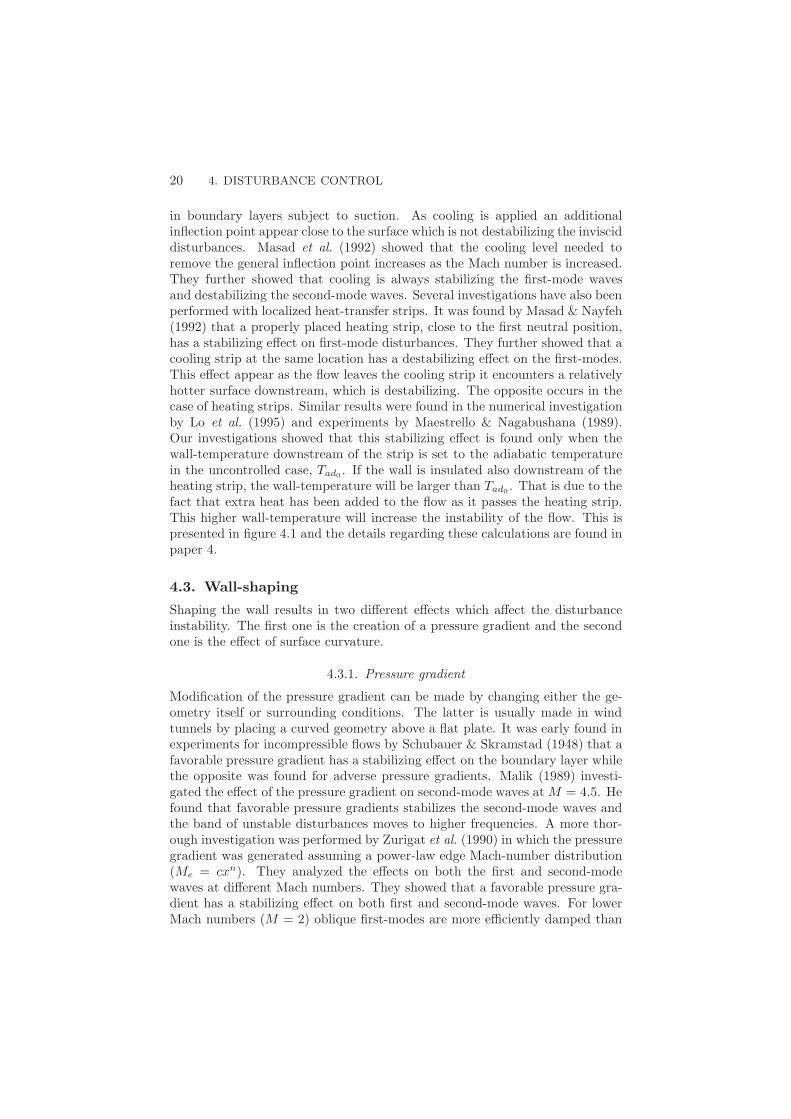
Figure 4.1. Disturbance control on a flat plate boundarylayer using a heating strip with a temperature of 1.5 timesthe adiabatic temperature when no control is applied, locatedat 720 + Re + 900. Left: Streamwise variation of the localgrowth rate of a 2D disturbance with F = 15 ( 10"6, for thecases of zero control (solid), compared to the cases when theheating strip is used and the plate downstream of the heatingstrip is assumed insulated (dash-dot), and heat transfer occurs(dash), M = 0.8, T# = 300 K, Pr = 0.72. Right: correspond-ing N -factors.
4.2. Wall coolingIt was early recognized that uniformly distributed cooling has a damping e!ecton viscous instabilities of boundary-layer flows at various Mach number, seeexperiments by e. g. Diaconis et al. (1957) and Jack et al. (1957). Liepmann &Fila (1947) showed that at low subsonic speeds the transition location on a flatplate moves upstream as it is heated. The destabilizing e!ect of wall-heatingon boundary-layer disturbances is due to the increase of the viscosity of airnear the wall, which creates inflectional velocity profiles there. Cooling thewall on the other hand, decrease the viscosity near the wall which results ina thicker velocity profile and thus a more stable flow. Lees & Lin (1946) andMack (1984) used inviscid and viscous stability theory, respectively, and foundthat subsonic air boundary layers can be completely stabilized by uniformlydistributed wall-cooling. Mack (1984) also showed that uniformly distributedcooling has a destabilizing e!ect on the higher modes. The results by Mack(1984) have also been confirmed in experiments for supersonic flows by Lysenko& Maslov (1984). In the work by Masad et al. (1992) similar results werefound using the spatial stability equations for compressible flows. Coolinghas an e!ect on the compressible boundary layer similar to the one found
20 4. DISTURBANCE CONTROL
in boundary layers subject to suction. As cooling is applied an additionalinflection point appear close to the surface which is not destabilizing the invisciddisturbances. Masad et al. (1992) showed that the cooling level needed toremove the general inflection point increases as the Mach number is increased.They further showed that cooling is always stabilizing the first-mode wavesand destabilizing the second-mode waves. Several investigations have also beenperformed with localized heat-transfer strips. It was found by Masad & Nayfeh(1992) that a properly placed heating strip, close to the first neutral position,has a stabilizing e!ect on first-mode disturbances. They further showed that acooling strip at the same location has a destabilizing e!ect on the first-modes.This e!ect appear as the flow leaves the cooling strip it encounters a relativelyhotter surface downstream, which is destabilizing. The opposite occurs in thecase of heating strips. Similar results were found in the numerical investigationby Lo et al. (1995) and experiments by Maestrello & Nagabushana (1989).Our investigations showed that this stabilizing e!ect is found only when thewall-temperature downstream of the strip is set to the adiabatic temperaturein the uncontrolled case, Tad0 . If the wall is insulated also downstream of theheating strip, the wall-temperature will be larger than Tad0 . That is due to thefact that extra heat has been added to the flow as it passes the heating strip.This higher wall-temperature will increase the instability of the flow. This ispresented in figure 4.1 and the details regarding these calculations are found inpaper 4.
4.3. Wall-shapingShaping the wall results in two di!erent e!ects which a!ect the disturbanceinstability. The first one is the creation of a pressure gradient and the secondone is the e!ect of surface curvature.
4.3.1. Pressure gradient
Modification of the pressure gradient can be made by changing either the ge-ometry itself or surrounding conditions. The latter is usually made in windtunnels by placing a curved geometry above a flat plate. It was early found inexperiments for incompressible flows by Schubauer & Skramstad (1948) that afavorable pressure gradient has a stabilizing e!ect on the boundary layer whilethe opposite was found for adverse pressure gradients. Malik (1989) investi-gated the e!ect of the pressure gradient on second-mode waves at M = 4.5. Hefound that favorable pressure gradients stabilizes the second-mode waves andthe band of unstable disturbances moves to higher frequencies. A more thor-ough investigation was performed by Zurigat et al. (1990) in which the pressuregradient was generated assuming a power-law edge Mach-number distribution(Me = cxn). They analyzed the e!ects on both the first and second-modewaves at di!erent Mach numbers. They showed that a favorable pressure gra-dient has a stabilizing e!ect on both first and second-mode waves. For lowerMach numbers (M = 2) oblique first-modes are more e"ciently damped than

4.3. WALL-SHAPING 21
0 0.1 0.2 0.3 0.4 0.50
4
8
12
16
20
24
NE
s/c
(a)
0 0.1 0.2 0.3 0.4 0.50
4
8
12
16
20
24
NE
s/c
(b)
Figure 4.2. E!ect of including curvature terms in the PSEon the disturbance growth. Envelope of envelopes of N -factor curves for cross-flow (CF) and Tollmien-Schlichting (TS)waves. (a) with curvature included; (b) without curvature inthe PSE. Traveling CF (Solid), stationary CF (dashed), 2DTS (dotted) and 3D TS (dash-dotted). Mean flow over infi-nite swept wing with leading edge sweep angle /le = 30.2o,Mach number M# = 0.8 and temperature T# = 230 K.
two-dimensional ones. For higher Mach-numbers (M = 4# 8) it was shown for2D second-mode waves that the damping e!ect of a favorable pressure gradientdecreases with increasing Mach number. For both disturbance types it wasshown that the maximum growth rate varies almost linearly with n.
4.3.2. Curvature
The e!ects of the curvature on the disturbance growth can roughly be dividedinto two categories, i. e. those by concave surfaces and those by convex surfaces.The interest here lies mainly in the case of convex surfaces as such geometrieshave been analyzed in this thesis. It should however be mentioned that stabil-ity analysis of boundary layer flows over concave surfaces has been the topicof many investigations as it concerns the problem of so called Gortler vortices,i. e. stationary counter-rotating vortices arising from centrifugal e!ects (see e.g. Hall 1983; Spall & Malik 1989). The case of convex surfaces was studied byMasad & Malik (1994) for three-dimensional incompressible flows over an infi-nite swept cylinder. They found that curvature is stabilizing both stationaryand traveling disturbances. Including nonparallel terms, on the other hand,is known to be destabilizing and will therefore have an opposite e!ect on thedisturbance growth compared to curvature. Masad & Malik (1994) found how-ever that the changes in disturbance growth in an analysis accounting for boththese e!ects will be controlled by the convex curvature part.

22 4. DISTURBANCE CONTROL
!
s/c0 0.1 0.2 0.3 0.4 0.5
0
10
20
30
40
50
Figure 4.3. Curvature, !, of the wing analyzed in Figure 4.2which is used to calculate the curvature radius 1/!.
In the parabolized stability equations used in this thesis, (2.18), the scalefactors hi and corresponding derivatives mij are all functions of the curvature !.An example on the e!ect of including curvature in (2.18) or not, is given here.The latter is obtained by setting h1 = h3 = 1, and corresponding derivativesto zero. The case is the mean flow on the upper surface of an infinite sweptwing (see Pralits & Hanifi 2003). Here the envelope of envelopes (EoE) ofthe N -factors for a large number of convectively unstable disturbances havebeen computed both with and without curvature terms in the linear stabilityequations. The results are given in Figure 4.2 where the horizontal axis showsthe arc-length of the surface divided by the chord length.
The mean flow pressure gradient is strong and negative upstream of s/c *0.4 and weak and positive downstream of this position. Due to the inflectionpoint in the velocity profile perpendicular to the inviscid streamline in theregion of a favorable pressure gradient, cross-flow (CF) waves are amplified.Further downstream, in the zero or weakly adverse pressure gradient region,Tollmien-Schlichting type of waves are amplified. The curvature ! of the wingcan be seen in Figure 4.3. Close to the leading edge the curvature is large andthen decreases rapidly downstream until approximately s/c = 0.05. Down-stream of this position the curvature is an order of magnitude smaller com-pared to the leading edge. As the region of large curvature coalesce with theregion of favorable pressure gradient it is clear that the disturbance growth ofCF waves, here given by the N -factors, will be mostly a!ected by the presenceof the curvature terms in the linear stability equations.

CHAPTER 5
Optimal design for disturbance control
The knowledge obtained from the analysis regarding disturbance control, whichwas previously described, can be used in design of di!erent active and passivedevices in order to a!ect the laminar portion of a geometry such as an aircraftwing. Using suction and blowing, or the wall temperature for control purposescan be considered as active devices. The term design here refers to how the massflux or temperature should be distributed along the surface. The knowledgeregarding the e!ect of the pressure distribution and curvature on disturbancegrowth can also be related to the design of the geometry itself. For a rigidbody this is made once and can be regarded as a passive control device. Astraight forward design approach is, for a given number of design variables,to perform a parameter study in order to find the “best” design. If we takethe example of design of a mass flux distribution, this means in practice totest di!erent control domains, mass flux amplitudes, distributions and furthermore, for each case compute the e!ect on the disturbance growth. This can bean extremely time-consuming approach if the number of degrees of freedom islarge. The word “best” is not objective and its meaning depends on the specificcase. For mass flux design it might be to decrease disturbance growth usingthe least amount of suction power, while for wing design the best could be todecrease disturbance growth while maintaining operational properties such asgiven lift, and pitch-moment coe"cients, and volume. The best solution froma parameter analysis however does not rule out the possibility that an evenbetter solution might exist.
A di!erent design approach is to define an optimization problem with anobjective function which includes the costs of the design that one wants tominimize using certain control or design variables. Conditions which should besatisfied while minimizing the objective function are introduced as constraints.The advantage of the latter approach is that a number of di!erent optimiza-tion techniques such as e. g. gradient-based and generic algorithms exist whichdepending on the problem can be used to e"ciently compute an optimal so-lution. Gradient-based algorithms are especially e"cient when the number ofobjective functions is small compared to the number of degrees of freedom.
5.1. BackgroundThe work related to design of active and passive control devices for distur-bance control and transition delay dates back several centuries, and a review
23

24 5. OPTIMAL DESIGN FOR DISTURBANCE CONTROL
is therefore not made here. Instead an attempt is made to cover representativeinvestigations where optimization techniques have been used for the purposeof disturbance control.
5.1.1. Natural laminar flow
Design of a geometry such that the laminar portion is increased or maximizedis commonly denoted Natural Laminar Flow (NLF) design. In terms of practi-cal implementations, NLF is probably the simplest approach. Once a feasiblegeometry is found no additional devices such as e. g. suction systems, sensorsor actuators need to be mounted. One approach to NLF design is, in a firststep, to generate a pressure distribution (target) that delays transition, then,in a second step, design a wing that results in a pressure distribution as closeas possible to the target. In addition constraints on e. g. lift, pitch, volume,minimum thickness et cetera must be handled. Green & Whitesides (1996)took an iterative approach which uses a target pressure-N-factor relationshipto compute the desired pressure distribution, and an inverse method to findthe geometry which satisfies the computed pressure distribution. The N -factormethod has also been used in multidisciplinary optimization problems of wholeaircraft configurations where aerodynamics is considered as one discipline. InLee et al. (1998), it was used to predict the onset of transition in order to deter-mine where to turn on a chosen turbulence model in the Reynolds-Averaged-Navier-Stokes equations, enabling calculation of the friction drag. In Manning& Kroo (1999), a surface panel method was coupled with an approximativeboundary layer calculation, and stability analysis. Note however, that none ofthese investigations explicitly calculates the sensitivity of a quantity obtainedfrom the stability analysis such as the N -factor or disturbance kinetic energy,with respect to variations of the geometry. In paper 5, the sensitivity of thedisturbance kinetic energy with respect to the geometry is used for the purposeof optimal NLF design.
5.1.2. Laminar flow control
Laminar flow control (LFC) is an active control technique, commonly usingsteady suction, to maintain the laminar state of the flow beyond the chordReynolds number at which transition usually occurs. It is one of the few con-trol techniques which has been attempted in flight tests. A combination ofNLF and LFC, where the active control is employed on a just a part of thesurface is called hybrid laminar flow control, HLFC. For an extensive reviewof these techniques see Joslin (1998). Most investigations of HLFC concernssuction but also wall-cooling have been used for control purposes. Balakumar& Hall (1999) used an optimization procedure to compute the optimal suctiondistribution such that the location of a target N -factor value was moved down-stream. The theory was derived for two-dimensional incompressible flows andthe growth of the boundary layer was not taken into account. In Airiau et al.

5.1. BACKGROUND 25
(2003), a similar problem was solved for the purpose of minimizing the distur-bance kinetic energy, accounting for the non-parallel e!ects using the Prandtlequations and the PSE for incompressible two-dimensional flows. The sameproblem is extended to three-dimensional incompressible flows in paper 2, andcompressible flows on infinite swept wings in paper 3. Similar investigationsfor the purpose of optimizing temperature distributions are, to the best of ourknowledge, not found in the literature. In Masad & Nayfeh (1992), a parametertest was performed to find the “best” location for a predefined temperature dis-tribution in order to reduce the N -factor of a given disturbance. In Gunzburgeret al. (1993) an optimal control problem using boundary controls for the incom-pressible full Navier-Stokes equations was derived. An application to control byheating and cooling was given with the wall heat flux as the control and a targetwall temperature as the objective. In paper 4, a problem is formulated for thepurpose of minimizing the disturbance kinetic energy by optimizing the walltemperature distribution. In Hill (1997b) an inverse method was mentioned tocompute the optimal suction distributions, and cooling/heating distributions,however no details were given there.
5.1.3. Control by blowing and suction
In a large number of investigations, di!erent optimal control strategies in a tem-poral frame work have been investigated. A recent thesis by Hogberg (2001)on the topic of optimal control of boundary layer transition provides a goodoverview of this field. The investigations considered here are performed forspatially developing flows. In Hogberg & Henningson (2001), an extension tospatially developing incompressible flows was made for previously developedoptimal feedback control through periodic blowing and suction at the wall.Even though parallel flow assumptions are needed for their formulation, suc-cessful results are shown for control of TS waves in Blasius flow and cross-flowvortices in Falkner-Skan-Cooke flow. Cathalifaud & Luchini (2000) formulatedan optimal control problem for laminar incompressible flows over flat-, andconcave walls with optimal perturbations. They successfully minimized boththe disturbance kinetic energy at a terminal position, and as streamwise inte-grated quantity, by optimizing distributions of blowing and suction. In Waltheret al. (2001) an optimal control problem was derived for two-dimensional in-compressible flows with the focus on minimizing the disturbance kinetic energyof TS waves. They accounted for the developing boundary layer using thePSE. In both of the latter investigations, adjoint equations were used to obtainsensitivities of the chosen objective function with respect to the control. Aglobal framework for feedback control of spanwise periodic disturbances, forspatially developing flows, was presented by Cathalifaud & Bewley (2002). Inpaper 1, we compute the sensitivity of the disturbance kinetic energy in a spa-tially developing boundary layer flow, with respect to periodic forcing at thewall and inside the boundary layer. The formulation is made using the PSEfor compressible flows and the sensitivities are computed using the adjoint ofthe PSE. The sensitivity of the disturbance kinetic energy with respect to the
26 5. OPTIMAL DESIGN FOR DISTURBANCE CONTROL
wall normal velocity component of the perturbation is used in section 5.4.2 toformulate an optimal control problem for cancellation of instability waves.
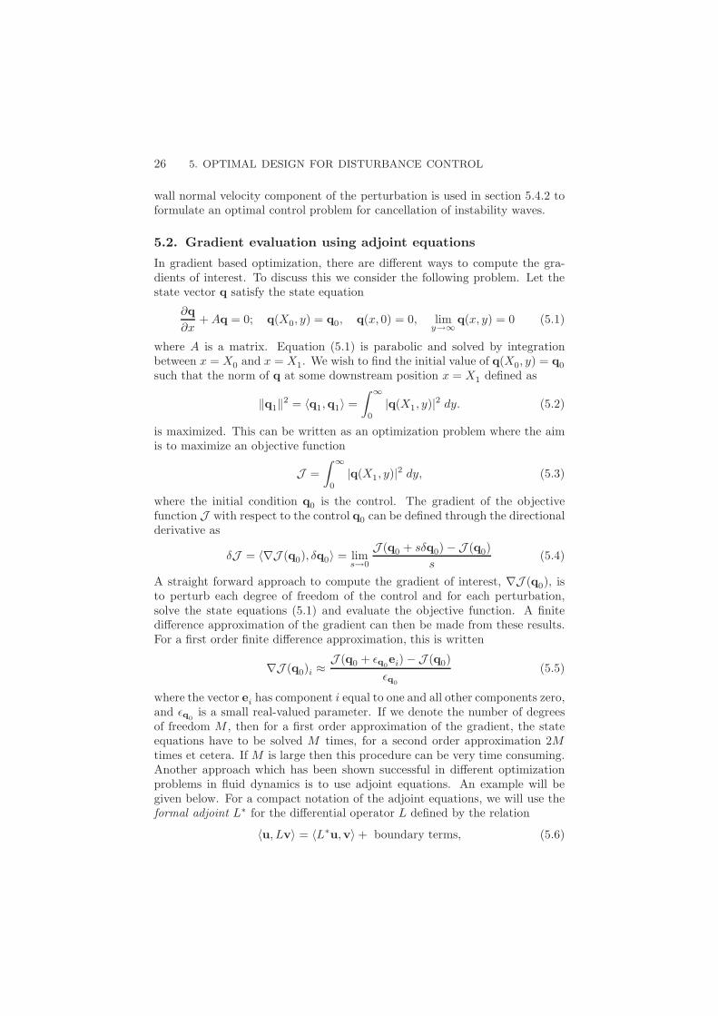
5.2. Gradient evaluation using adjoint equationsIn gradient based optimization, there are di!erent ways to compute the gra-dients of interest. To discuss this we consider the following problem. Let thestate vector q satisfy the state equation
!q!x
+ Aq = 0; q(X0, y) = q0, q(x, 0) = 0, limy%#
q(x, y) = 0 (5.1)
where A is a matrix. Equation (5.1) is parabolic and solved by integrationbetween x = X0 and x = X1. We wish to find the initial value of q(X0, y) = q0
such that the norm of q at some downstream position x = X1 defined as
,q1,2 = -q1,q1. =* #
0|q(X1, y)|2 dy. (5.2)
is maximized. This can be written as an optimization problem where the aimis to maximize an objective function
J =* #
0|q(X1, y)|2 dy, (5.3)
where the initial condition q0 is the control. The gradient of the objectivefunction J with respect to the control q0 can be defined through the directionalderivative as
0J = -"J (q0), 0q0. = lims%0
J (q0 + s0q0)# J (q0)s
(5.4)
A straight forward approach to compute the gradient of interest, "J (q0), isto perturb each degree of freedom of the control and for each perturbation,solve the state equations (5.1) and evaluate the objective function. A finitedi!erence approximation of the gradient can then be made from these results.For a first order finite di!erence approximation, this is written
"J (q0)i *J (q0 + .q0
ei)# J (q0).q0
(5.5)
where the vector ei has component i equal to one and all other components zero,and .q0
is a small real-valued parameter. If we denote the number of degreesof freedom M , then for a first order approximation of the gradient, the stateequations have to be solved M times, for a second order approximation 2Mtimes et cetera. If M is large then this procedure can be very time consuming.Another approach which has been shown successful in di!erent optimizationproblems in fluid dynamics is to use adjoint equations. An example will begiven below. For a compact notation of the adjoint equations, we will use theformal adjoint L$ for the di!erential operator L defined by the relation
-u, Lv. = -L$u,v.+ boundary terms, (5.6)

5.2. GRADIENT EVALUATION USING ADJOINT EQUATIONS 27
where the inner product -·, ·. is defined as
-u,v. =* X1
X0
* #
0uTv dx dy (5.7)
for Rn-valued vectors u and v. Here, the superscript $ stands for the adjointquantities and T for the transpose. The derivation of the adjoint equationsis made in the following steps: the first variation of equations (5.3) and (5.1)gives
0J (q0) = 2* #
0q(X1, y)T0q(X1, y) dy, (5.8)
!0q!x
+ A0q = 0, 0q(X0, y) = 0q0, 0q(x, 0) = 0, limy%#
0q(x, y) = 0 (5.9)
Then (5.9) is multiplied with the co-state or adjoint variable r and used inthe inner product given by (5.7). The right hand side of (5.6) is derived byremoving the derivatives from 0q using partial integration
-r, !0q!x
+ A0q. = -# !r!x
+ ATr, 0q. +!* #
0rT 0q dy
"X1
X0. (5.10)
We now require r to satisfy the adjoint equation with the initial and boundaryconditions
# !r!x
+ ATr = 0, r(X1, y) = 2q(X1, y), r(x, 0) = 0, limy%#
r(x, y) = 0.
(5.11)Equation (5.11) is integrated from x = X1 to x = X0 and the initial conditionfor r at x = X1 is chosen such that the remaining boundary terms can bewritten* #
0r(X0, y)T 0q(X0, y) dy. = 2
* #
0q(X1, y)T 0q(X1, y) dy = 0J (q0) (5.12)
Since the left hand side of (5.12) is equal to 0J , the gradient of J with respectto q0 is identified as
"J (q0) = r(X0, y) (5.13)Compared to the finite-di!erence approach, the gradient (5.13) is now evalu-ated by solving the state equation (5.1) and the corresponding adjoint equation(5.11) once, independent of the size of M . The right hand side of (5.6) canbe derived using either a continuous or discrete approach. A continuous ap-proach means that the adjoint equations are derived from the continuous stateequation and then discretized. In the discrete approach, the adjoint equationsare derived directly from the discretized state equation. The gradient whichis later identified from the adjoint equations, should in the latter case havean accuracy close to machine precision. The accuracy of the gradient derivedusing the continuous approach increases as the resolution of the computationaldomain is increased. This is well explained in Hogberg & Berggren (2000). Thecontinuous approach has been used through out the thesis except for the workin paper 5 where the adjoint of the inviscid flow equations are derived using

28 5. OPTIMAL DESIGN FOR DISTURBANCE CONTROL
the discrete approach. The accuracy of the numerically calculated gradients isdiscussed in papers 1, 2 and 5.
5.3. Outline of the current approachIn this section the optimal design problems considered in this thesis are out-lined. Gradient-based optimization is used in all cases and the gradients ofinterest are evaluated from the solution of the adjoint equations. The aim isto use di!erent control or design variables in order to achieve a decrease indisturbance growth and therefore an increase in the laminar portion, thus adecrease in friction drag.
5.3.1. Objective function
The objective function is given as the sum of the di!erent costs of the statewhich we want to minimize in order to achieve some desired goal. The costs,or cost functions, can be given di!erent weights depending on their respectiveimportance for the goal. In the analysis given here, the cost of friction drag isnot given as a measure of the shear stress. It is instead based on the idea thatan increase in the laminar portion of the body will result in a decrease of thefriction drag. This can also be seen as moving the position of laminar-turbulenttransition further downstream. The cost function is therefore a measure whichcan be related to the transition position. One choice is to measure the kineticenergy of a certain disturbance at a downstream position, say Xf . This can bewritten as
Ef =12
* Z1
Z0
* +#
0qHM q h1dx2dx3
11111x1=Xf
, (5.14)
where q = (", u, v, w, T )T and M = diag(0, 1, 1, 1, 0) which means that thedisturbance kinetic energy is calculated from the disturbance velocity compo-nents. If the position Xf is chosen as the upper branch of the neutral curve,then the measure can be related to the maximum value of the N -factor as
Nmax = ln
#Ef
E0
, (5.15)
where E0 is the disturbance kinetic energy at the first neutral point. If inaddition, the value of the N -factor of the measured disturbance is the onewhich first reaches the transition N -factor, then the position can be relatedto the onset of laminar-turbulent transition. It is however not clear, a priori,that such a measure will damp the chosen disturbance or other ones in thewhole unstable region, especially if di!erent types of disturbances are present.For Blasius flow, it has been shown that a cost function based on a singleTS wave is su"cient to successfully damp the growth of other TS waves (seePralits et al. 2002; Airiau et al. 2003). On a swept wing however, it is commonthat both TS and cross-flow waves are present and moreover can be amplifiedin di!erent streamwise regions. An alternative is therefore to measure the

5.3. OUTLINE OF THE CURRENT APPROACH 29
kinetic energy as the streamwise integral over a defined domain. Using such anapproach several di!erent disturbances, with respective maximum growth rateat di!erent positions, can be accounted for in one calculation. Here, the size ofK disturbances superimposed on the mean flow at an upstream position X0,is measured by their total kinetic energy as
E! =K%
k=1
12
* Xme
Xms
* Z1
Z0
* +#
0qH
k M qkh1dx1dx2dx3. (5.16)
We now define the objective function as the sum of all the cost functions basedon the disturbance kinetic energy as
Jq = ,E! + (1 # ,)Ef , (5.17)
where the parameter , can be chosen between zero and one, depending onthe quantity we want to minimize. An alternative approach to decrease thedisturbance growth and thus increase the laminar portion of the wing was in-vestigated in Airiau et al. (2003) to optimize the mean flow suction distributionin a given domain. They minimized the streamwise integral of the shape factor,which for 2D disturbances in a 2D boundary layer should result in a suppressionof disturbance amplification. Minimizing the shape factor is a more heuristicapproach based on the knowledge that in such flows the two-dimensional dist-urbances are stabilized by any thinning of the boundary layer. Their resultsshowed that an optimal suction distribution based on minimizing the shape fac-tor does have a damping e!ect on the disturbance growth. A negative aspectof not explicitly minimizing a measure of the disturbances is that one cannotknow if the optimized control will have a damping e!ect on the disturbances.This has to be calculated after wards. A cost function based on the streamwiseintegral of the shape factor is here written as
JQ =* Xme
Xms
H12h1dx1 =* Xme
Xms
0102
h1dx1, (5.18)
where both the displacement 01, and momentum-thickness 02 are based on thevelocity component which is in the direction of the outer streamline. In paper3 we present results which show that optimal suction distributions obtainedby minimizing expression (5.18) does not have a damping e!ect, but insteadamplifies disturbances in the case of swept wing flows.
5.3.2. Optimal design cases
With the objective functions defined, di!erent optimal design cases can be out-lined. We consider the flow over a body decomposed into three di!erent parts:a steady inviscid part provides a pressure distribution P for a given geometryx, a steady mean flow Q is the solution for a given pressure distribution andgeometry, and the solution q emerging from the stability analysis calculated fora given mean flow and geometry. From the latter, the objective function basedon the disturbance kinetic energy can be evaluated. If the objective function

30 5. OPTIMAL DESIGN FOR DISTURBANCE CONTROL
Design variables Euler BLE PSE Obj. fcns. Gradients
ww P0 % Q0 % q% Jq "Jq(ww)mw, Tw P0 % Q% q% Jq "Jq(mw), "Jq(Tw)mw, Tw P0 % Q% JQ "JQ(mw), "JQ(Tw)
x P % Q% q% Jq "Jq(x)x P % Q% JQ "JQ(x)x P % JP "JP (x)
Table 5.1. Table of state equations involved in the possibleoptimal design cases. The arrows indicates the order in whichthe equations are solved, and P , Q, and q are the states ob-tained by solving the Euler, BLE and PSE respectively. Thesubscript 0 means that the solution is fixed during the opti-mization procedure.
is based on the shape factor, only the inviscid and mean flow parts are consid-ered. Three di!erent types of control or design variables are used. In the first,we consider unsteady forcing such as periodic blowing/suction at the wall, ww,for a fixed geometry. In this case, only the stability equations are a!ected bythe control as the inviscid flow and mean flow are both time-independent andnon-linear e!ects are not accounted for. As a second case we consider controlof disturbances by modifications of the mean flow on a fixed geometry. Thisis made using either a mass flux distribution mw or a wall temperature dis-tribution Tw. Here both the mean flow and disturbances are a!ected by thecontrol, which means that an objective function can be based on either Q orq. The last case considers optimal design by changing the geometry and willa!ect all states, i. e. the inviscid flow, the mean flow, and the disturbances. Itis therefore possible to consider objective functions based on either of the threestates P , Q or q.
If we denote the objective functions based on the three di!erent statesP , Q, and q as JP , JQ, and Jq respectively, a chart of possible optimaldesign problems can be made. This is shown in table 5.1. The solution ofthe inviscid flow, mean flow and disturbances are here denoted Euler, BLEand PSE, respectively. Depending on the design case, one or several stateswill change during the optimization. The states which are not changed (keptfixed) in respective case are given subscript 0. The di!erent gradients requiredto solve respective optimization problem are given in the column on the righthand side of table 5.1.

5.4. OPTIMAL LAMINAR FLOW CONTROL 31
5.4. Optimal laminar flow control5.4.1. Sensitivity analysis using periodic forcing
The concept of wave cancellation was discussed in section 4.1 and exampleswere given of experimental results using di!erent types of forcing, or actuatorssuch as heating plates, vibrating ribbons, and blowing and suction. Beforedeciding which actuator to use in order to control the instability waves, it canbe of interest to investigate the sensitivity of di!erent types of forcing 1 on ameasure of the disturbance growth of a given disturbance. The latter is heregiven by the objective function Jq, expression (5.17). A small variation of theforcing 01 will cause a small variation of the objective function 0Jq and thegradient "Jq(1) express the sensitivity of Jq with respect to 1. The di!erentforcing considered here are the disturbance velocity components uw, vw, ww
and temperature Tw at the wall, and a momentum force S inside the boundarylayer as the model of a vibrating ribbons. When a low amplitude periodicforcing such as blowing/suction at the wall is applied, only the linear stabilityequations need to be considered, as neither the mean flow nor the inviscidflow is a!ected if non-linear interaction of the disturbances are neglected. Thestate equations solved here are the parabolized stability equations outlined insection 2.4, which including the above mentioned periodic forcing are written
LP q = S, (5.19)* +#
0qH !q
!x1dx3 = 0. (5.20)
The forcing given at the wall are introduced as boundary conditions in (5.19).The gradients of the objective function with respect to each forcing are derivedusing adjoint equations. This is described in detail in paper 1 and the gradientswith respect to the wall forcing are
"Jq(uw) =µD3(u$)
$Re, "Jq(vw) =
µD3(v$)$Re
,
"Jq(ww) =""$
$, "Jq(Tw) = #$D3('$)
$PrRe,
where $ = ei", and with respect to the momentum forcing
"Jq(S) =q$
$where q$ = ("$, u$, v$, w$, '$)T.
Here, the over bar denotes the complex conjugate and superscript / denoteadjoint variables. The latter satisfy the adjoint of the parabolized stabilityequations (APSE), here given as
L$P q$ = S$
P (5.21)
!
!x1
* +#
0q$H !LP
!(q h1h2h3 dx3 = f$, (5.22)

32 5. OPTIMAL DESIGN FOR DISTURBANCE CONTROL
(a)
Re
fd, !R = 10
adj, !R = 10
fd, !R = 20
adj, !R = 20
fd, !R = 50
adj, !R = 50
(b)
Re
!R = 10
!R = 20
!R = 50
200 400 600 8000
1
2
3
200 400 600 80010−6
10−5
10−4
10−3
10−2
10−1
Figure 5.1. Comparison between adjoint (adj) and centraldi!erence (fd) calculations for di!erent %R. Mach numberM = 0.7, ) = 0. (a) lines denote ||(!Jq/!wr, !Jq/!wi)/%n||and symbols |"Jq(ww)n|. (b) relative error.
Details regarding equations (5.21)–(5.22) are found in paper 1 for the case ofJq = Jq(, = 0). The adjoint equations shown here are derived from thecontinuous state equations. An alternative is to first discretize the state equa-tions and then derive the adjoint equations. It was concluded by Hogberg &Berggren (2000) that a continuous formulation is a good enough approximationif control is performed on a problem with a dominating instability. This typeof analysis can be made with the PSE and a continuous approach is there-fore used here. In order to verify the accuracy of the gradient, we comparethe gradients computed using the adjoint equations with those obtained usinga finite-di!erence approximation. In the latter, the gradient of the objectivefunction with respect to each forcing is approximated by a second-order accu-rate central finite-di!erence scheme. To compare the gradients given by theadjoint and finite-di!erence approaches let us consider the example of a wallnormal velocity perturbation 0ww at x3 = 0. The variation of Jq with respectto this wall perturbation is :
0Jq =!Jq
!wr0wr +
!Jq
!wi0wi
The subscripts r and i denote the real and imaginary parts of a complex num-ber. In the finite-di!erence approach, the variation of Jq is obtained by im-posing the inhomogeneous boundary condition ww = ±2 at x1 = x1
n. Here, 2is a small number and index n refers to n-th streamwise position. Then, theapproximative gradients are calculated using a second-order accurate finite-di!erence scheme. The expression for 0Jq in the adjoint approach, for a flatplate geometry, is in discretized form given as
0Jq =* Z1
Z0
N"1%
n=2
12("Jq(ww)Hn0wwn + c.c.)%n dx2,

5.4. OPTIMAL LAMINAR FLOW CONTROL 33
100 200 300 400 500 600 700 8000
0.125
0.25
100 200 300 400 500 600 700 8000
0.005
0.01
0.015
100 200 300 400 500 600 700 8000
0.001
0.002
0.003
100 200 300 400 500 600 700 8000
0.0025
0.005(a) (b)
(c) (d)
Re Re
! = 0
! = 0.02
! = 0.04
Figure 5.2. Modulus of the gradients (sensitivities) due to2D and 3D wall forcing as a function of the Reynolds numberfor a flat plate boundary layer at Mach number M = 0.7.(a) |"Jq(uw)|, streamwise velocity component; (b) |"Jq(vw)|spanwise velocity component; (c) |"Jq(ww)| normal velocitycomponent; (d) |"Jq(Tw)| temperature component. The +marks the first and second neutral point for each case.
where %n = (x1n+1 # x1
n"1)/2 and c.c. is the complex conjugate. In the fol-lowing, the quantity "Jq(ww)n is compared to those of the finite-di!erenceapproach. The case is a flat plate boundary layer with free stream Mach num-ber of 0.7, and the streamwise domain used here is Re ' [250, 750]. The mod-ulus ||(!Jq/!wr, !Jq/!wi)/%n||, as a function of x1
n, is shown in figure 5.1aand is compared to |"Jq(ww)n| for di!erent resolution of the streamwise step%R. A good agreement is found between the approaches for a given %R, andboth values converge as %R is decreased. The relative error given in figure5.1b is below half a percent for all cases and decreases as %R is decreased.Sensitivity results for a flat plate boundary layer at Mach number M = 0.7subject to two-, and three dimensional wall forcing by uw, vw, ww and Tw canbe seen in figure 5.2. Here the modulus of each component have been plottedas a function of the local Reynolds number. For all cases except the spanwise

34 5. OPTIMAL DESIGN FOR DISTURBANCE CONTROL
Euler BLE PSE
APSE
wk+1w
"J kq (ww)
Figure 5.3. Flow chart for the case of minimizing the distur-bance kinetic energy using the wall normal disturbance veloc-ity at the wall ww.
component, the largest sensitivity is obtained for two-dimensional wall forcingand the maximum value occurs close to the first neutral point of analyzed dis-turbance. It can also be seen that the magnitude of the wall normal velocitycomponent is about 15 times that of the streamwise component for this caseand the ratio is even larger compared to the spanwise velocity component andthe temperature. This implies that blowing/suction is the most e"cient meanof controlling instability waves. However, as shown in paper 1, the sensitivitydecreases with increasing Mach number.
5.4.2. Wave cancellation
In principle, any periodic forcing considered in section 5.4.1 can be optimized.However, as an example we choose the wall normal velocity component becauseit has been shown to give the highest sensitivity, and also because it is a goodmodel for periodic blowing/suction. In order to find the optimal solution for alimited cost of the control, and also to bound the control amplitude we definean objective function which balances the cost of the kinetic energy and thecontrol as
Jq = Jq + l2* X1
X0
|ww|2 h1 dx1. (5.23)
The term l2 serve as a penalty on the control such that l2 = 0 means unlimitedcontrol and vice verse. The gradient of the objective function (5.23) withrespect to the control is given as
"Jq(ww) = "Jq(ww) + 2 l2ww (5.24)
As the optimization problem is defined for a given geometry and mean flow, theonly state equation which is updated in the optimization procedure is the PSE(5.19)-(5.20). The optimization procedure can now be described considering thechart given in figure 5.3 where k is the iteration number of the optimizationloop. An initial disturbance q0 is superimposed on the mean flow at an initialposition X0. The PSE is integrated from x = X0 to x = X1 and the objectivefunction is evaluated. The adjoint equations, APSE are then integrated fromx = X1 to x = X0. The gradient is evaluated from the solution of the APSE

5.4. OPTIMAL LAMINAR FLOW CONTROL 35ln$
E(x
1)/
E0(x
1)
ampl
itud
eRe Re
500 1000 1500 2000−5
−4
−3
−2
−1
0
1B2 B1 B1−opt (a)
500 1000 1500 2000
−1
−0.5
0
0.5
1
x 10−5
(b)
B1
Figure 5.4. Control of a two-dimensional wave with F =30 ( 10"6 in a zero pressure gradient flat plate boundarylayer where M# = 0. (a) energy for zero (solid) and optimal(dashed) control, (b) the optimal suction/blowing distributiongiven as |ww| (solid) and Real(ww) (dashed). Bi and Bi-optmark the branch points for zero and optimal control
and the new boundary condition for the PSE is calculated using a chosenoptimization algorithm. In the next loop, the PSE is solved with a new ww
followed by the APSE. The optimization loop is continued until the variationof the objective function is less than a prescribed value. Results of the optimaldesign problem described above are given in figure 5.4 for the case when Jq =Jq(, = 0). Here we consider a flat plate boundary layer with free stream Machnumber M# = 0 and zero pressure gradient. The computational domain inthe streamwise direction is Re = [350, 1750]. A two-dimensional disturbancewith reduced frequency F = 30 ( 10"6 is superimposed on the meanflow atRe = 350. The control is imposed along the whole plate and the penalty hasvalue of l = 104. The objective function is evaluated at Re = 1750 which isclose to the second branch of the neutral curve, i. e. where the disturbancekinetic energy is close to its maximum. In figure 5.4a the reduction in energyhas been plotted as the natural logarithm of the ratio between the square rootof optimal-, and initial disturbance kinetic energy, ln
$E(x1)/E0(x1). Branch
1 and 2 of the uncontrolled case have been marked with vertical lines as B1 andB2, respectively. The downstream shift of branch one in the case of optimalcontrol is shown with a vertical line marked B1 # opt. In figure 5.4b theoptimal distribution of suction and blowing is plotted both as the real partand absolute value. Here it is seen that the control acts most strongly in thevicinity of the first neutral point and then decays rapidly both in the upstreamand downstream direction. Results showing that the disturbance kinetic energymeasured close to the second branch of the neutral curve is most sensitive toperiodic forcing close to the first branch of the neutral curve can be seen inpaper 1 for di!erent Mach numbers.

36 5. OPTIMAL DESIGN FOR DISTURBANCE CONTROL
5.4.3. Hybrid laminar flow control
The motivation for using optimal control theory for the purpose of hybrid lam-inar flow is that in many industrial applications (see Joslin 1998), the designof e. g. suction systems rely on the experience of the engineers which may notalways give the largest delay of laminar-turbulent transition at a given suctionpower. Design using steady forcing implies that given a fixed geometry, themean flow will change during the optimization procedure. The analysis here ismade using either the wall mass flux mw = "wWw, or the wall temperature Tw
as design variables. This particular choice is made as both mw and Tw havebeen investigated for the purpose of Hybrid Laminar Flow Control. As out-lined in table 5.1, several di!erent cases can be considered depending on whichcombination of objective function and control variable that is used. Gradientbased optimization is used in all cases analyzed here and the gradients areevaluated from the solution of adjoint equations. When the objective functionis evaluated from the solution of the mean flow, JQ, then only the BLE is usedin the optimization and the gradient of JQ with respect to the chosen controlvariable is evaluated from the adjoint of the boundary layer equations (ABLE).Minimization of Jq on the other hand, requires the solution of both the BLEand PSE and the respective gradients are evaluated from the ABLE which inturn is forced by the solution of the APSE. A summary on how to computethe gradient for the di!erent cases is given in table 5.2 where W $ and T $ aresolutions of the ABLE. Details regarding respective equation are given in pa-pers 3 and 4. Note that for the cases presented in table 5.2 the assumption ismade that the streamwise domain of the forcing and the objective function isthe same. If this is not the case, changes occur in the boundary conditions ofboth the BLE and ABLE. This is covered in paper 3 and 4.
5.4.3.1. Limiting the control
In many optimization problems it is of interest to bound or limit the control,and in such a way compute the optimal solution using the least e!ort. Otherarguments for bounding the control come from issues regarding validity of thestate equations or avoiding ill-posed problems. This can be made using e. g.a regularization parameter such that the objective function express the sumof the original measure, expression (5.17) or (5.18), and a parameter times adefined measure of the control. An example was given in section 5.4.2 for thecase of optimizing periodic blowing/suction. As an example here, we considerthe case of optimization the wall mass flux to minimize the disturbance kineticenergy. A new objective function can be written
Jq = Jq + l2* X1
X0
m2w h1 dx1. (5.25)
The only di!erence compared to the equations given in table 5.2 appear in theexpression of the gradient which is now given as
"Jq(mw) = "Jq(mw) + 2 l2mw. (5.26)

5.4. OPTIMAL LAMINAR FLOW CONTROL 37
Des. Euler BLE PSE Obj. APSE ABLE Gradients
mw P0 % Q% q% Jq q$ % Q$ % "Jq(mw) = W $w
mw P0 % Q% JQ Q$ % "JQ(mw) = W $w
Tw P0 % Q% q% Jq q$ % Q$ % "Jq(Tw) =$
Re Pr!T $
w
!x3
Tw P0 % Q% JQ Q$ % "JQ(Tw) =$
Re Pr!T $
w
!x3
Table 5.2. Table of state and adjoint equations to evaluaterespective gradient in the optimal design cases using steadyforcing. The arrows indicates the order in which the equationsare solved. P , Q, and q are the states obtained by solving theEuler, BLE and PSE respectively, and Q$ and q$ are solutionsof the ABLE and APSE respectively. The subscript 0 definesthat the solution is fixed during the optimization procedure.
If the regularization parameter l is zero then the control is unbounded, andwhen l > 0 then it is bounded. In practice this means that as l is increased, lesscontrol e!ort is allowed, and possibly less decrease in the original state measureis obtained. In some cases it is of interest not only to bound the control butmore specifically bound it at a certain value. One example is when the massflux is optimized for disturbance control purposes. The suction distributionis commonly obtained by a system of pumps and pipes which uses a certainamount of energy. It can therefore be of interest to find an optimal suctiondistribution which uses a specified amount of energy EC , which for instancecan be written as
EC =* X1
X0
m2w h1 dx1. (5.27)
In this case the problem is not regularized but instead constrained. As shownin papers 3 and 4, this constraint can be fulfilled using a Lagrange multipliertechnique. Details on the derivations are found in the papers and the resultinggradient expression is
"Jq(mw) = "Jq(mw) + 2 3$mw, (5.28)
The constant regularization parameter l2 in (5.26) has now been replaced byan adjoint variable 3$. This adjoint variable can be solved as follows: when"J (mw) = 0 then mw = #W $
w/(232) is the corresponding optimal mass fluxdistribution and usually denoted optimality condition, mw is then substituted

38 5. OPTIMAL DESIGN FOR DISTURBANCE CONTROL
JQ(/) Jq(/)
"J k# (/)
/k+1
Euler BLE PSE
APSEABLE
Figure 5.5. Optimization procedure using steady forcing.Here, k denotes the iteration number, / is the control vari-able, JQ and Jq are the objective functions evaluated fromthe solutions of the BLE and PSE respectively.
into (5.27) and an expression for 3$ is evaluated as
3$ =
+1
4EC
* X1
X0
W $2w h1dx1
, 12
. (5.29)
It should be noted that using this approach does not mean that expression(5.27) is satisfied in each iteration of the optimization procedure. The con-straint on the control energy is derived assuming that "J (mw) = 0. There-fore, as the optimization problem converge, i. e. "J (mw) goes to zero, also theconstraint on the control energy will converge.
5.4.3.2. Solution procedure
The optimization procedures for the di!erent optimal design problems consid-ered here can be described using the chart in figure 5.5. There, k denotesthe iteration number, / is the control variable, JQ and Jq are the objectivefunctions evaluated from the solutions of the BLE and PSE respectively. Westart by considering the case of minimizing Jq for a single disturbance, i. e.K = 1 if Jq includes expression (5.16). This case is presented figure 5.5 as thelarge dotted rectangle. The optimization is performed for a given geometryand inviscid solution in an iterative procedure. During each iteration step, weperform successive calculations of the BLE and PSE from X0 to X1; and APSEand ABLE from X1 to X0. Then, a new control variable /k+1 is computedusing the gradient evaluated from the solution of the ABLE, in a chosen opti-mization algorithm. The calculations are repeated until the relative change inthe objective function is less than a prescribed value. If the objective functionincludes expression (5.16) with K > 1 then instead of solving both state andadjoint equations K times, we can utilize the fact that the ABLE, here written

5.4. OPTIMAL LAMINAR FLOW CONTROL 39
0 1 2 3 410−4
10−3
10−2
10−1
100
iteration
|" J
|/|"
J0|
500 600 700 800 900 10001.04
1.06
1.08
1.1
Re
Tw
0 1 2 3 460
70
80
90
100
iteration
J
0 1 2 3 40
0.2
0.4
0.6
0.8
iteration
Ec
GivenCalculated
(a) (b)
(c) (d)
Figure 5.6. Convergence history for the case of minimizingthe disturbance kinetic energy at a downstream position us-ing the wall temperature. (a) objective function vs. iterationnumber, (b) wall temperature vs. Reynolds number for all it-erations, the arrow shows the direction of increasing iterationnumber (c) control energy, given and calculated vs. iterationnumber, (d) gradient norm normalized by its initial value vs.iteration number.
as
L$B Q$ = S$
B. (5.30)
are linear equations. In this case the gradient is evaluated as follows: the BLEis solved once; the PSE and APSE are solved K times; the right hand side ofthe ABLE, S$
B, is calculated as
S$B =
K%
k=1
S$Bk
.
Finally, the gradient is evaluated from a single calculation of the ABLE. Thecase of minimizing JQ is computationally less expensive. This case is shown infigure 5.5 as the smaller dotted rectangle. During each iteration step, successivecalculations are performed of the BLE from X0 to X1; and ABLE from X1 toX0. The gradient evaluation and convergence is then as described above.

40 5. OPTIMAL DESIGN FOR DISTURBANCE CONTROL
5.4.3.3. Convergence
An example of the convergence history for an optimal design case is shownin figure 5.6. The wall temperature distribution is optimized such that thedisturbance kinetic energy at a downstream position is minimized on a flatplate with zero pressure gradient and a free stream Mach number M# = 0.7.A disturbance with reduced frequency F = 50 ( 10"6 is superimposed onthe meanflow at Re = 500 and the objective function, given by expression(5.14), is evaluated at Re = 935. The wall temperature distribution Tw isoptimized between Re = 545 and Re = 935, and the convergence criteria isset as (J k+1
q # J kq )/J k
q < 10"4. When control is applied, a deviation of thewall temperature, %Tw, occur with respect to the case of zero control. Theconstraint used here is the square of %Tw, accounting for both heating andcooling, integrated in the control domain. With the reference temperaturetaken as the adiabatic wall temperature in the case of zero control Tad0
, this iswritten
EC =* Xce
Xcs
&Tw # Tad0
(x1, 0)'2
dx1, (5.31)
Here, the start and end of the control domain are denoted Xcs and Xce, re-spectively, and the value of EC used in this example is 0.5. The optimizationalgorithm used here is the L-BFGS-B1 routine and convergence was reachedafter 4 iterations. The objective function and the norm of the gradient, nor-malized by its initial value, both as functions of the iteration number can beseen in figures 5.6a and b, respectively. The objective function has reached aplateau while the gradient norm is still decreasing indicates that the solutionis getting close to a local minimum. At the last iteration the relative di!erencebetween the given and calculated control energy is 10"4 (figure 5.6c). If theoptimization is continued then finally it would reach a point where the gradi-ent norm would no longer decrease. This might depend on the accuracy of thegradient and/or the search algorithm used. The results from iteration 3 and 4are not possible to distinguish from each other which can be seen in figure 5.6b,and as e"ciency is of importance when a large number of designs are evaluated,the results here are considered converged.
5.4.3.4. HLFC for an industrial application
Optimization of the wall temperature or the mass flux distribution withoutconsidering how it can implemented and used in a real case might solely beof academic interest or serve as a reference case. This has been addressed inpaper 3 for the case of optimizing the mass flux distribution for the purpose ofdisturbance control on infinite swept wings. The direct application of such ananalysis is a tool which could be used in design of HLFC systems. The mass
1The algorithm is the limited memory quasi-Newton method developed by Zhu et al. (1994).It is based on a limited memory BFGS approximation of the Hessian matrix of the functionalf , and a gradient projection method is used to account for bounds on the data which makesit suitable for large scale problems where only the gradient of f is available.
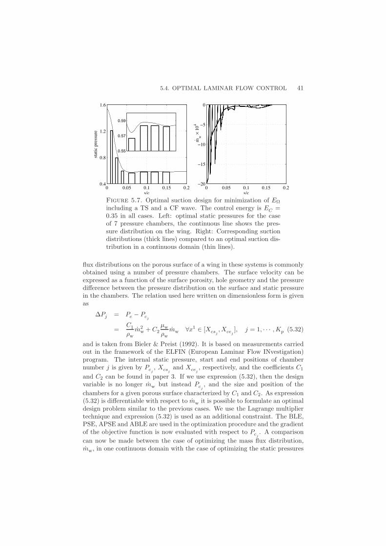
5.4. OPTIMAL LAMINAR FLOW CONTROL 41
0 0.05 0.1 0.15 0.20.4
0.8
1.2
1.6
static
pre
ssur
e
s/c
0.55
0.57
0.59
0 0.05 0.1 0.15 0.2−20
−15
−10
−5
0
mw
# 1
04s/c
.
Figure 5.7. Optimal suction design for minimization of E!
including a TS and a CF wave. The control energy is EC =0.35 in all cases. Left: optimal static pressures for the caseof 7 pressure chambers, the continuous line shows the pres-sure distribution on the wing. Right: Corresponding suctiondistributions (thick lines) compared to an optimal suction dis-tribution in a continuous domain (thin lines).
flux distributions on the porous surface of a wing in these systems is commonlyobtained using a number of pressure chambers. The surface velocity can beexpressed as a function of the surface porosity, hole geometry and the pressuredi!erence between the pressure distribution on the surface and static pressurein the chambers. The relation used here written on dimensionless form is givenas
%Pj = Pe # Pcj
=C1
"w
m2w + C2
µw
"w
mw 0x1 ' [Xcsj, Xcej
], j = 1, · · · , Kp (5.32)
and is taken from Bieler & Preist (1992). It is based on measurements carriedout in the framework of the ELFIN (European Laminar Flow INvestigation)program. The internal static pressure, start and end positions of chambernumber j is given by Pcj
, Xcsjand Xcej
, respectively, and the coe"cients C1
and C2 can be found in paper 3. If we use expression (5.32), then the designvariable is no longer mw but instead Pcj
, and the size and position of thechambers for a given porous surface characterized by C1 and C2. As expression(5.32) is di!erentiable with respect to mw it is possible to formulate an optimaldesign problem similar to the previous cases. We use the Lagrange multipliertechnique and expression (5.32) is used as an additional constraint. The BLE,PSE, APSE and ABLE are used in the optimization procedure and the gradientof the objective function is now evaluated with respect to Pcj
. A comparisoncan now be made between the case of optimizing the mass flux distribution,mw, in one continuous domain with the case of optimizing the static pressures

42 5. OPTIMAL DESIGN FOR DISTURBANCE CONTROL
0 0.1 0.2 0.3 0.4 0.50
4
8
12
16
20
NE
s/c
CF TS
Figure 5.8. Envelope of envelopes (EoE) of N -factor curvesfor the cases of zero control (dotted) and the optimal pressurechambers in figure 5.7 (solid). A comparison is made with theEoE of NE-factor curves (dashed) obtained with the continu-ous suction distribution in figure 5.7.
in a number of discrete pressure chambers, with the aim of minimizing thedisturbance kinetic energy. In the latter, mw is indirectly optimized through therelation (5.32). Results taken from paper 3 of such a comparison are presentedhere for the case of minimizing the disturbance kinetic energy calculated as thesum of a Tollmien-Schlichting (TS) and cross-flow (CF) wave. The mean flowstudied is the boundary layer on the upper side of a swept wing designed forcommercial aircraft. The continuous mass flux distribution is optimized in thewhole available control domain. A configuration of seven pressure chambersare used for the comparison and the start of the first, and end of the lastpressure chamber are given by the end points of the available control domain.In both the continuous and pressure chamber cases, the control energy (5.27)is kept constant with a value of 0.35. The left hand side of figure 5.7, shows theoptimal static pressures for the case of 7 chambers. The pressure distributionof the wing has been added for comparison in the plot. The largest values of%Pj occur close to the leading edge and then decrease downstream. This ismost evident observing the close up made in each plot on the left hand side.The corresponding suction distributions are shown on the right hand side of thesame figure. There a comparison is made with the case of optimizing the massflux in a continuous control domain. Both the continuous suction distributionand the ones obtained from the optimal static pressures are larger in magnitudeupstream and then decrease rapidly and become almost constant downstream.The e!ect on the disturbance growth is given in figure 5.8 by plotting theenvelope of envelopes (EoE) of the N -factor curves both for TS and CF waves,for the cases of zero and the optimal suction distributions shown in figure 5.7.The results using the continuous suction distribution can be seen as a referencecase of what best can be achieved. As further constraints are imposed using

5.5. SHAPE OPTIMIZATION FOR NATURAL LAMINAR FLOW 43
the pressure chambers, it is expected that less damping of the disturbances willbe achieved.
5.5. Shape optimization for natural laminar flowThe various possible optimal design cases which can be considered in the currentframe work, where outlined in table 5.1. In the cases of using the shape of thegeometry as design variables, it was shown that the objective function can bebased on either the inviscid, mean flow, or stability solution. Note, that inaddition, also combinations of the three can be used as an objective function,see paper 5. An objective function based on the solution of the inviscid flow, JP ,is commonly used in the case of shape optimization where the aim is to minimizee. g. the pressure, or wave drag. References to optimization problems regardinginviscid flows can be found in e. g. Jameson (1988). A design problem whichaccounts for viscous flow e!ects can be formulated using either JQ, and/orJq as objective function. In particular the latter enables the possibility toaccount for the physics related to laminar-turbulent transition. In the currentapproach there are several physical approximations made. A discussion aboutthis is found in paper 5. The goal of the approach taken is to use an iterativegradient-based optimization procedure with the aim of minimizing an objectivefunction based on a measure of the linear disturbance growth by optimizing theshape of the geometry, such as a wing. As a decrease in disturbance growthmeans a downstream shift of the laminar-turbulent transition location, andthus an increase of the laminar portion of the surface, the approach taken herecan be seen as optimal design for natural laminar flow.
5.5.1. Problem formulation and gradients
We minimize the objective function based on the disturbance kinetic energyJq, expression (5.17), which depends explicitly on the solution of the stabilityequations q and the mesh, here given by the nodal coordinates X. This is herewritten as
J 1 J (q,X) , (5.33)and is evaluated as follows:
1. The solution of the Euler equations for compressible flows (see paper 5)provides the pressure distribution of a given geometry
2. The viscous mean flow is obtained by solving (2.5)–(2.8) for the givengeometry, and the pressure distribution from the Euler solution.
3. The parabolized stability equations (2.18)–(2.19) are solved for the ge-ometry, and mean flow from the boundary layer analysis.
4. The objective function (5.33) is evaluated from the solution of the parab-olized stability equations.
If w, Q, and q are the solutions of the three state equations given above, thenJ can be considered to be a functional of X only and the objective functionis then denoted JX(X). The nodal coordinates, X, are evaluated from the

44 5. OPTIMAL DESIGN FOR DISTURBANCE CONTROL
displacements, y, of the nodes on the airfoil by a mesh movement algorithm,here denoted X 1 X(y). The displacements are controlled by the parametera, i. e. y 1 y(a). From these definitions we can now define
Jy (y) = JX (X (y)) , and Ja (a) = Jy (y (a)) , (5.34)
which clearly shows that Ja (a) is the objective function depending only on thecontrol parameter a. As the gradient of Ja (a) with respect to a is used in theoptimization procedure, we show in paper 5 that "Ja can be evaluated from
"JX % "Jy % "Ja,
in the above mentioned order. The gradient of the objective function withrespect to the nodal coordinates "JX is derived using adjoint equations and isevaluated solving the APSE, ABLE and adjoint of the Euler equations (AEuler)in the mentioned order.
5.5.2. Mesh displacements, parametrization andgeometrical constraints
All displacements are made with respect to a reference mesh, defined by itsvector of nodal coordinates X0. For a vector yk of shape displacements thenew grid is obtained as
Xk = X0 + Lyk . (5.35)Given the gradient "JX of a functional JX of the nodal coordinates, the gradi-ent of the functional Jy (X) 1 JX (X (y)) is obtained by the following matrix–vector product
"Jy = LT"JX . (5.36)Smooth shapes, together with geometric constraints, are obtained taking thevectors of displacements y that are the solutions of a minimization problem(see Amoignon 2003) of the form
y =
2minv&Rn
12vT Asv # vT Msa ,
CT y = b,(5.37)
where As is the sti!ness matrix associated with the Laplace operator, Ms isa mass matrix, C is the matrix whose rows are the gradients of the linearconstraints (in Rn'm) and b is the vector of values imposed to the constraints(in Rm). The solution y to the above system can be seen as the vector ofdisplacements, which, according to the norm defined by the positive definitematrix As, is the closest to the solution of the discretized Laplace equationdefined by
Asy = Msa , (5.38)and fulfills exactly the constraints
CTy = b . (5.39)
Such a parameterization implies that the controls are the vector a, right handside of equation (5.38), and the vector b, right hand side of the constraints,

5.5. SHAPE OPTIMIZATION FOR NATURAL LAMINAR FLOW 45
2Euler BLE PSE
APSEABLEAEuler
ak+1% yk+1% Xk+1
"J ka 3 "J k
y 3 "J kX
Figure 5.9. Flow chart for the case of minimizing the dis-turbance kinetic energy using the parameter a to control theshape of geometry.
relation (5.39). The gradients with respect to a and b, which are the controlvariables in our method, can then be obtained by solving an adjoint problem(see Amoignon 2003) of the form
-AT
s #C#CT 0
.-y$
#$
.=-"Jy
0
., (5.40)
from which it holds that
"Ja = MTs y$ and "Jb = ##$ . (5.41)
Note that "Jy in (5.40) is obtained by evaluating expression (5.36). All con-straints considered so far are equality constraints, and b is therefore a vectorof constants. The only control parameter in this case is therefore a.
5.5.3. Solution procedure
A simple chart of the order in which the state and adjoint equations are solvedand gradients are evaluated in order to perform optimal NLF is given in fig-ure 5.9. There, k denotes the iteration number and the procedure is as follows:
1. For k = 1, we start with an initial Euler mesh X0
2. The Euler, BLE and PSE are solved in the given order3. The objective function J k is evaluated4. The adjoint equations, APSE, ABLE and AEuler are solved5. The gradients "J k
X , "J ky and "J k
a are evaluated in the given order6. A new control parameter ak+1 is calculated2 using the gradient "J k
a
7. If k > 1, check convergence: If |(J k+1 # J k)/J k| < ., else3 continue8. A new mesh Xk+1 is calculated from the new control parameter ak+1
9. Goto 2.
2In the computations shown in paper 5, the L-BFGS-B routine was used, normally requiringseveral functional and gradient evaluations in order to build up the approximative Hessianmatrix.3Several convergence criteria exist in the L-BFGS-B routine, (see Zhu et al. 1994)

46 5. OPTIMAL DESIGN FOR DISTURBANCE CONTROL
5.5.4. An optimal design case
An optimization case in which constraints are not imposed on operational prop-erties such as lift, and pitch-moment coe"cients might result in a design whichis not useful. Results are shown here for the case of minimizing an objectivefunction including both the disturbance kinetic energy, pressure drag CD, andin addition penalties on the deviations of the lift, and pitch-moment coe"cients,CL and CM , from the initial values. This is written
JC = #UJ + #DCD + #L123CL # C0
L
42 + #M123CM # C0
M
42, (5.42)
where the coe"cients #U and #D are used to normalize J and CD with respec-tive values computed using the initial mesh. The coe"cients #L and #M areused to penalize the deviations of CL and CM from respective values computedon the initial mesh. The initial design is the RAE2822 airfoil and the flowis characterized by a free stream Mach number of M# = 0.734 and Reynoldsnumber of Re# = 6.5(106. The disturbance used to evaluate J has a physicalfrequency f$ = 11 kHz and wave angle of /w * 40( and is integrated from closeto the leading edge to half chord. As geometrical constraints we impose thatthe volume should not deviate from its initial value and that a region aroundthe leading edge is kept fixed.
0 2 4 6 8 10 12 14 16
10−2
10−1
100
J q
iteration
Disturbance kinetic energy
0 2 4 6 8 10 12 14 1670
80
90
100
110
120
130
104 .C
D
iteration
Wave drag
Figure 5.10. Left: Disturbance kinetic energy. Right: wavedrag. Both as functions of the iteration number.
Results of the convergence history is shown in figures 5.10 and 5.11 for thedisturbance kinetic energy, pressure drag, lift, and pitch-moment coe"cientsas functions of the iteration number. A reduction in the objective function(5.42) is obtained from the first to the last iteration (see paper 5). During afew iterations, however, it can be noted that the pressure drag increase whilethe deviations of CD and CM decrease, figure 5.10. At the final iteration a

5.5. SHAPE OPTIMIZATION FOR NATURAL LAMINAR FLOW 47
0 2 4 6 8 10 12 14 160.2
0.3
0.4
0.5
0.6
0.7
0.8
0.9
iteration
Lift and pitch moment
Figure 5.11. Lift, (triangle-solid) and pitch-moment (circle-solid) coe"cients as functions of the iteration number. Thevalues at initial design are indicated at each step (solid).
reduction has been obtained in both disturbance kinetic energy and pressuredrag while CD and CM are kept within a few percent, figure 5.11.
A comparison between the pressure coe"cients, and geometry for the initial(solid) and last iteration (dash) obtained from the optimization can be seen infigure 5.12. The largest change in the geometry occur in the region on the upperside of the airfoil where J is evaluated. This can also be seen in the pressuredistributions. The relative small change on the lower side is caused in order tosatisfy the constant volume constraint. As the upper side of the final designis thinner, and the part around the leading edge is fixed to approximately 4%chord, an increase occur in the curvature of the airfoil around 10% chord. Thiscan be seen in the decrease in the pressure coe"cient in that region.
The EoE of the N -factor curves for a large number of modes can be seenin figure 5.13 for the initial and final design. In comparison with figure 5.12we can note that the pressure gradient in the region where the disturbancebecome unstable has change from an adverse to zero or weakly favorable. Thishas a damping e!ect on the disturbance growth in the whole domain where Jis evaluated, which can be seen in figure 5.13. In order to estimate the changein the total drag computations were performed solving the Reynolds AveragedNavier Stokes equations on the initial and final design. The transition locationin these computations was estimated using the EoE curves computed using thepressure distributions from the Euler solutions. The computations showed adecrease in pressure drag of about 25%, viscous drag of about 23%, and totaldrag of about 24%. In the approach taken here there are still improvementsto be made. This can for instance be seen looking at the region x/c * 0.4 tox/c * 0.6 of the pressure distributions in figure 5.12 of the final design. The

48 5. OPTIMAL DESIGN FOR DISTURBANCE CONTROL
0 0.2 0.4 0.6 0.8 1−1.5
−1
−0.5
0
0.5
1
1.5
−Cp
x/c
Pressure coefficients
0 0.2 0.4 0.6 0.8 1−0.08
−0.06
−0.04
−0.02
0
0.02
0.04
0.06
0.08
y/c
x/c
Airfoils
Figure 5.12. Left: Pressure coe"cients for initial (solid), andfinal design (dash) obtained from the optimization solving theEuler equations. A comparison is made using the ReynoldsAveraged Navier Stokes Equtions to compute the flow of theinitial (dash-dot), and final design (dot). Right: initial (solid)and final design (dash).
0 0.1 0.2 0.3 0.4 0.50
1
2
3
4
5
6
NE
s/c
Envelope of envelope of N−factor curves
Figure 5.13. Envelope of envelopes of N -factor curves. Linescorrespond to the cases shown in figure 5.12.
pressure gradient in this region is adverse indicating that separation occurs.More results and discussions are found in paper 5.

CHAPTER 6
Summary & conclusions
The work presented in this thesis concerns the use of gradient-based optimiza-tion techniques for the purpose of laminar flow control (LFC), and design ofwings for natural laminar flow (NLF). The goal of using this technique is toreduce the viscous drag. Reduction of viscous drag can be seen as an in-crease of the laminar portion of the wing, thus a delay of laminar-turbulenttransition. On wings in low free-stream turbulence environments, the latter isusually caused by break down of small disturbances which grow as they prop-agate down stream. The fluid flow has been divided into three di!erent parts,namely: an inviscid part providing the pressure distribution for a given geome-try, a viscous mean flow which is computed given the pressure distribution andgeometry, and finally a linear stability analysis using the PSE providing thegrowth rate of convectively unstable disturbances superimposed on the viscousmean flow. The growth rate can been used to predict the transition locationusing the so called eN -method. Here it is assumed that transition will occur atthe location where the total amplification of the disturbance, with respect tothe first streamwise position where the disturbance starts to grow, attains anempirically determined value, whose logarithm is generally denoted by N .
Several optimization problems have been defined for the purpose of LFCand NLF with the aim of minimizing an objective function based on measuresof, or related to, the growth of unstable disturbances. Here, di!erent controlvariables, means of control, have been used and the gradients of the objectivefunction with respect to the control has been derived using adjoint equations.Especially the derivation of the adjoint of the PSE (APSE), and the adjointof the BLE (ABLE) for compressible flows have been of interest, and nowaccomplished can be used in several applications. An existing optimizationroutine has been used in most cases as the topic of this research does notconcern development of these routines.
The accuracy of the gradients evaluated from the solution of the adjointequations have been investigated by comparing them with those computedby a finite-di!erence approximation. The tests have shown that an increasedaccuracy can be achieved by increasing the spatial resolution of the discretizedequations. As the latter is known to cause numerical stability problems forthe PSE, a known method to overcome this problem has been used which alsoalters the APSE and ABLE. A sensitivity analysis using the gradients of thedisturbance kinetic energy at the second neutral point with respect to periodic
49

50 6. SUMMARY & CONCLUSIONS
forcing show that control is most e"ciently made in the vicinity of the firstneutral point. It was further shown that the disturbance kinetic energy is mostsensitive to control by means of periodic blowing and suction, and in generalthe e"ciency decreases with increasing Mach number.
Results of optimal steady suction distributions have been presented forboth incompressible and compressible flows. It has been shown that minimiz-ing an objective function based on the disturbance kinetic energy of a singledisturbance results in a suction distribution which has a damping e!ect on alarge number of disturbances of the same type, e. g. (TS) Tollmien-Schlichting-,or (CF) cross-flow waves. On swept wings, a situation might occur when boththese types of waves exist simultaneously. For such cases it has been shownthat both types must be included in the objective function in order to obtain asuction distribution which has a damping e!ect on other disturbances of thesetwo types. Results of optimal temperature distributions for disturbance controlhave been presented for various Mach numbers. It has been shown that the e"-ciency of the optimal control decreases when the wall temperature downstreamof the control domain is maintained at its original adiabatic value, comparedto the case when the wall there is insulated. It has also been shown that thee"ciency decreases with increasing Mach number.
A problem has been formulated to perform optimal NLF design, in whichthe aim is to minimize a measure of the disturbance kinetic energy. Results havebeen presented for cases where both the disturbance kinetic energy, and wavedrag have been reduced simultaneously while lift, and pitch-moment coe"cientsas well as the volume have been maintained at desired values.
One of the goals with work presented here was to show that the derivedtechniques can be used in realistic applications. This was addressed for the caseof optimal suction distributions in which the problem was also formulated usingdiscrete pressure chambers, and computations were made on an infinite sweptwing designed for commercial aircraft. Also the problem of optimal NLF designwas formulated such that airfoils in realistic flow conditions can be optimized.
Acknowledgment
I want to thank my advisor Professor Dan Henningson for being so supportive,encouraging and always available to assist in questions regarding the world offluid mechanics as well as personal matters. It has been a long and interestingjourney and I consider myself fortunate for the freedom I have been given toproceed, with my sometimes endless derivations, knowing that there was alwayssupport.
I want to thank my assistant advisor Doctor Ardeshir Hanifi for sharing hisknowledge as well software which has given me a very good basis from whichto start this work. He has spend many hours explaining theoretical matters,supporting me in the European projects and been a really good friend.
I want to thank Doctor Martin Berggren for many useful discussions whichhave provided more consistency in the mathematical formulations regardingthe adjoint equations.
I want to acknowledge Professor Alessandro Bottaro and Doctor ChristopheAiriau for the good cooperation which started in 1999, and the hospitality theyshowed me during my stay in Toulouse in October, 2000.
This work has been funded by the Swedish Foundation for Strategic Re-search (SSF) through the Integral Vehicle Structures (IVS)-program and par-tially by the Swedish Defence Research Agency (FOI), and the EU project(ALTTA contract G4RD-CT-2000-00143).
I want to acknowledge the colleagues in the ALTTA project for all theinteresting discussions as well as good company.
Many thanks to everyone at the Department of Mechanics for the goodcompany, fika, innebandy and nice atmosphere. In particular I want to men-tion: Luca Brandt (V), Markus Hogberg, Ruben Wetind, Martin Skote, NuliferIpek, Astrid Herbst, Ori Levin, Jerome Hoep!ner, Mattias Chevalier, GustafMartensson, Arnim Bruger, Johan Gullman-Strand, Fredrik Lundell, BjornLindgren och Jens Fransson.
Thanks Olivier for the good collaboration we had working on SEBAS.En stor kram till min familj och vannerna i sodertalje och ett speciellt tack
till FF&SB.
Karimah, gioia della mia vita, grazie che tu esisti : 4
51

Bibliography
Airiau, C. 2000 Non-parallel acoustic receptivity of a Blasius boundary layer usingan adjoint approach. Flow, Turbulence and Combustion 65, 347–367.
Airiau, C., Bottaro, A., Walther, S. & Legendre, D. 2003 A methodologyfor optimal laminar flow control: Application to the damping of Tollmien-Schlichting waves in a boundary layer. Phys. Fluids 15, 1131–1145.
Al-Maaitah, A. A., Nayfeh, A. H. & Masad, J. A. 1991 E!ect of suction on thestability of supersonic boundary layers. part I: Second-mode waves. J. FluidsEngng 113, 591–597.
Amoignon, O. 2003 Aerodynamic shape optimization: I. Tech. Rep.. Departmentof Information Technology, Uppsala, Sweden, licenciate thesis to be published,University of Uppsala.
Andersson, P., Henningson, D. S. & Hanifi, A. 1998 On a stabilization procedurefor the parabolic stability equations. J. Engng Maths 33, 311–332.
Arnal, D. 1993 Boundary layer transition: Predictions based on linear theory. Spe-cial course on ’progress in transition modeling’, March-April 1993. AGARD-R-793, 2-1–2-63.
Balakumar, P. & Hall, P. 1999 Optimum suction distribution for transition pre-diction. Theor. Comput. Fluid Dyn. 13, 1–19.
Bertolotti, F. P. 1998 The influence of rotational and vibrational energy relaxationon boundary-layer stability. J. Fluid Mech. 372, 93–118.
Bertolotti, F. P., Herbert, T. & Spalart, S. 1992 Linear and nonlinear stabilityof the Blasius boundary layer. J. Fluid Mech. 242, 441–474.
Bieler, H. & Preist, J. 1992 HLFC for commercial aircraft. In First european forumon laminar flow technology , pp. 193–199. Hamburg.
Brandt, L. 2003 Numerical studies of bypass transition in the Blasius boundarylayer. PhD thesis, Royal Institute of Technology, Stockholm, Sweden.
Cathalifaud, P. & Bewley, T. R. 2002 A numerically tractable global frameworkfor the feedback control of boundary-layer perturbations. ASME, ASME FluidsEngineering Division Summer Meeting, Montreal, Canada.
Cathalifaud, P. & Luchini, P. 2000 Algebraic growth in a boundary layer: optimalcontrol by blowing and suction at the wall. Eur. J. Mech. B/Fluids 19 (4), 469–490.
Diaconis, N. S., Jack, J. R. & Wisniewski, R. J. 1957 Boundary-layer transition
52

BIBLIOGRAPHY 53
at mach 3.12 as a!ected by cooling and nose blunting. NACA Tech. Note No.3928 .
Dobrinsky, A. & Collis, S. S. 2000 Adjoint parabolized stability equations forreceptivity prediction. AIAA Paper (2000-2651).
Gaster, M. 1974 On the e!ect of boundary layer growth in flow stability. J. FluidMech. 66, 465–480.
Gedney, C. J. 1983 The cancellation of a sound-excited Tollmien-Schlichting wavewith plate vibration 26 (5), 1158–1160.
Green, B. E. & Whitesides, J. L. 1996 A method for the constrained design ofnatural laminar flow airfoils. AIAA Paper (96-2502).
Gunzburger, M. D., Hou, L. S. & Svobodny, T. P. 1993 The approximationof boundary control problems for fluid flows with an application to control byheating and cooling. Comp. Fluids 22 (2/3), 239–251.
Haj-Hariri, H. 1994 Characteristics analysis of the parabolized stability equations.Stud. Appl. Math. 92, 41–53.
Hall, P. 1983 The linear development of gortler vortices in growing boundary layers.J. Fluid Mech. 130, 41–58.
Hanifi, A., Henningson, D. S., Hein, S. & Bertolotti, F. P.and Simen, M.1994 Linear non-local instability analysis - the linear NOLOT code. FFA TN1994-54.
Hein, S., Bertolotti, F. P., Simen, M., Hanifi, A. & Henningson, D. S. 1994Linear non-local instability analysis - the linear NOLOT code. DLR-IB 223-94A 43.
Herbert, T. 1997 Parabolized stability equations. Annu. Rev. Fluid Mech. 29, 245–283.
Herbert, T. & Bertolotti, F. P. 1987 Stability analysis of nonparallel boundarylayers. Bull. Am. Phys. Soc. 32, 2079.
Hill, D. C. 1997a Receptivity in non-parallel boundary layers. In ASME FluidsEngineering Division Summer Meeting, FEDSM ’97 .
Hill, D. C. 1997b Inverse design for laminar three-dimensional boundary layers.Bull. Am. Phys. Soc. 42, 2120.
Hogberg, M. 2001 Optimal control of boundary layer transition. PhD thesis, RoyalInstitute of Technology, SE-172 90 Stockholm, Sweden.
Hogberg, M. & Berggren, M. 2000 Numerical approaches to optimal control ofa model equation for shear flow instabilities. Flow, Turbulence and Combustion65, 299–320.
Hogberg, M. & Henningson, D. S. 2002 Linear optimal control applied to insta-bilities in spatially developing boundary layers. J. Fluid Mech. 470, 151–179.
van Ingen, J. L. 1956 A suggested semiempirical method for the calculation of theboundary layer transition region. Tech. Rep. VTH-74. Department of Aeronau-tical Engineering, University of Delft.
Itoh, N. 1986 The origin and subsequent development in space of Tollmien-Schlichting waves in a boundary layer. Fluid Dyn. Res. pp. 119–130.
Jack, J. R., Wisniewski, R. J. & Diaconis, N. S. 1957 E!ects of extreme surfacecooling on boundary-layer transition. NACA Tech. Note No. 4094 .
Jameson, A. 1988 Aerodynamic design via control theory. J. Scientific Computing3 (3), 233–260.

54 BIBLIOGRAPHY
Jiang, L., Chang, C.-L., Choudhari, M. & Liu, C. 2003 Cross-validation of DNSand PSE results for instability-wave propagation in compressible boundary layerspast curvilinear surfaces. AIAA Paper (2003-3555), 33rd AIAA Fluid DynamicsConference and Exhibit, Orlando, Florida, 23-26 June, 2003.
Joslin, R. 1998 Overview of laminar flow control. Tech. Rep. 1998-208705. NASA,Langley Research Center, Hampton, Virginia.
Kozlov, V. V. & Levchenko, V. Y. 1985 Laminar-turbulent transition control bylocalized disturbances. AIAA Paper (85–0568).
Lee, J.-M., Schrage, D. P. & Mavris, D. N. 1998 Development of subsonic trans-ports with laminar flow wings. AIAA Paper (98-0406).
Lees, L. & Lin, C. C. 1946 Investigation of the stability of the laminar boundarylayer in a compressible fluid. NACA Tech. Note No. 1115 .
Levin, O. & Henningson, D. S. 2003 Exponential vs algebraic growth and transitionprediction in boundary layer flow. Flow, Turbulence and Combustion Acceptedfor publication.
Li, F. & Malik, M. R. 1994 Mathematical nature of parabolized stability equa-tions. In 4th IUTAM Symp. on Laminar-Turbulent Transition, Sendi, Japan(ed. R. Kobayashi), pp. 205–212. Springer.
Li, F. & Malik, M. R. 1996 On the nature of PSE approximation. Theor. Comput.Fluid Dyn. 8, 253–273.
Liepmann, H. W., Brown, G. L. & Nosenchuck, D. M. 1982 Control of laminar-instability waves using a new technique. J. Fluid Mech. 118, 187–200.
Liepmann, H. W. & Fila, G. H. 1947 Investigations of e!ects of surface temperatureand single roughness elements on boundary-layer transition. NACA Tech. ReportNo. 890 .
Lo, C. F., Lafrance, R., Meredith, W. S. & Wiberg, C. G. 1995 Laminar flowcontrol with wall temperature distribution for quiet supersonic wind tunnels.AIAA Paper (95-2296).
Lysenko, V. I. & Maslov, A. A. 1984 The e!ect of cooling on supersonic boundary-layer stability. J. Fluid Mech. 147, 39–52.
Mack, L. M. 1977 Transition prediction and linear stability theory. Paris: AGARDReport No 224, also JPL Publication 77-15, 1977.
Mack, L. M. 1984 Boundary-layer linear stability theory. AGARD Report No. 709 .
Mack, L. M. 1988 Stability of three-dimensional boundary layers on swept wings attransonic speeds. In IUTAM Symp. Transsonicum III (ed. J. Zierep & H. Oertel).Gottingen: Springer.
Maestrello, L. & Nagabushana, K. A. 1989 Relaminarization of turbulent flowon a flat plate by localized surface heating. AIAA Paper (89-0985), 2nd ShearFlow Conference, March 13-16, 1989/Tempe, AZ.
Malik, M. R. 1989 Prediction and control of transition in supersonic and hypersonicboundary layers. AIAA J. 27, 1487–1493.
Malik, M. R. & Balakumar, P. 1992 Nonparallel stability of rotating disk flowusing PSE. In Instability, Transition and Turbulence (ed. M. Hussaini, A. Kumar& C. Streett), pp. 168–180. Springer.
Manning, V. M. & Kroo, I. M. 1999 Multidisciplinary optimization of a naturallaminar flow supersonic aircraft. AIAA Paper (99-3102).

BIBLIOGRAPHY 55
Masad, J. A. & Malik, M. R. 1994 E!ects of body curvature and nonparllelism onthe stability of flow over a swept cylinder. Phys. Fluids 6, 2363–2379.
Masad, J. A. & Nayfeh, A. H. 1992 Laminar flow control of subsonic boundarylayers by suction and heat-transfer strips. Phys. Fluids A 4 (6), 1259–1272.
Masad, J. A., Nayfeh, A. H. & Al-Maaitah, A. A. 1991 E!ect of suction onthe stability of supersonic boundary layers. part II: First-mode waves. J. FluidsEngng 113, 598–601.
Masad, J. A., Nayfeh, A. H. & Al-Maaitah, A. A. 1992 E!ect of heat transferon the stability of compressible boundary layers. Comp. Fluids 21 (1), 43–61.
Matsubara, M. & Alfredsson, P. 2001 Disturbance growth in boundary layerssubjected to free-stream turbulence. J. Fluid Mech. 430, 149–168.
Milling, R. W. 1981 Tollmien-Schlichting wave cancellation 24 (5), 979–981.Pralits, J. O., Airiau, C., Hanifi, A. & Henningson, D. S. 2000 Sensitivity anal-
ysis using adjoint parabolized stability equations for compressible flows. Flow,Turbulence and Combustion 65 (3), 321–346.
Pralits, J. O. & Hanifi, A. 2003 Optimization of steady suction for disturbancecontrol on infinite swept wings. Phys. Fluids 15 (9), 2756–2772.
Pralits, J. O., Hanifi, A. & Henningson, D. S. 2002 Adjoint-based optimizationof steady suction for disturbance control in incompressible flows. J. Fluid Mech.467, 129–161.
Pruett, C. D. & Chang, C.-L. 1993 A comparison of PSE and DNS for high-speed boundary-layer flows. In Transitional and Turbulent Compressible Flows(ed. L. Kral & T. Zang), , vol. 151, pp. 57–67. Washington, D.C.: ASME.
Saric, W. S. & Nayfeh, A. H. 1975 Non-parallel stability of boundary layer flows.Phys. Fluids 18, 945–950.
Schubauer, G. B. & Skramstad, H. K. 1948 Laminar-boundary-layer oscillationsand transition on a flat plate. NACA Tech. Note No. 909 .
Simen, M. 1992 Local and non-local stability theory of spatially varying flows. InInstability, Transition and Turbulence (ed. M. Hussaini, A. Kumar & C. Streett),pp. 181–201. Springer.
Smith, A. M. O. & Gamberoni, N. 1956 Transition, pressure gradient and stabilitytheory. Tech. Rep. ES 26388. Douglas Aircraft Co.
Spall, R. E. & Malik, M. R. 1989 Goertler vortices in supersonic and hypersonicboundary layers. Phys. Fluids A 1, 1822.
Thomas, A. S. W. 1983 The control of boundary-layer transition using a wave-superposition principle. J. Fluid Mech. 137, 233–250.
Walther, S., Airiau, C. & Bottaro, A. 2001 Optimal control of Tollmien-Schlichting waves in a developing boundary layer. Phys. Fluids 13, 2087–2096.
Westin, K., Boiko, A., Klingmann, B., Kozlov, V. & Alfredsson, P. 1994Experiments in a boundary layer subjected to free stream turbulence. part 1.boundary layer structure and receptivity. J. Fluid Mech. 281, 193–218.
Zhu, C., Byrd, R., Lu, P. & Nocedal, J. 1994 L-BFGS-B: Fortran subroutinesfor large scale bound constrained optimization. Tech. Rep. NAM-11. EECS De-partment, Northwestern University.
Zurigat, Y. H., Nayfeh, A. H. & Masad, J. A. 1990 E!ect of pressure gradienton the stability of compressible boundary layers. AIAA Paper (90-1451), 21stFluid Dynamics, Plasma Dynamics and Lasers Conference, Seattle, WA.

56 BIBLIOGRAPHY

Part 2
Papers


Paper 1
1


Sensitivity Analysis Using Adjoint ParabolizedStability Equations for Compressible Flows
By Jan O. Pralits1,3, Christophe Airiau2,Ardeshir Hanifi3 and Dan S. Henningson1,3
An input/output framework is used to analyze the sensitivity of two- and threedimensional disturbances in a compressible boundary layer for changes in wall-and momentum forcing. The sensitivity is defined as the gradient of the kineticdisturbance energy at a given downstream position with respect to the forc-ing. The gradients are derived using the parabolized stability equations (PSE)and their adjoint (APSE). The adjoint equations are derived in a consistentway for a quasi two-dimensional compressible flow in an orthogonal curvilinearcoordinate system. The input/output framework provides a basis for optimalcontrol studies. Analysis of two-dimensional boundary layers for Mach num-bers between 0 and 1.2 show that wall- and momentum forcing close to branchI of the neutral stability curve give the maximum magnitude of the gradient.Forcing at the wall gives the largest magnitude using the wall normal velocitycomponent. In case of incompressible flow, the two-dimensional disturbancesare the most sensitive ones to wall inhomogeneity. For compressible flow, thethree-dimensional disturbances are the most sensitive ones. Further, it is shownthat momentum forcing is most e!ectively done in the vicinity of the criticallayer.
1. IntroductionTransition from laminar to turbulent flow can be triggered by unstable distur-bances inside the boundary layer. The growth of such1 disturbances are knownto be sensitive to surface inhomogeneities, forcing inside the boundary layerand external acoustic perturbations, see e.g. Nishioka and Morkovin (1986),Saric (1993) and Corke, Bar-Sever and Morkovin (1986). The studies devotedto the birth of disturbances due to such forcing are called receptivity. Theacoustic receptivity is explained by Goldstein (1983) as a wavelength conver-sion mechanism. The long wave length of an acoustic wave can be convertedto a shorter wave length of an instability wave at the leading edge or where
1Department of Mechanics, KTH, SE-100 44 Stockholm, Sweden.2Institut de Mecanique des Fluides de Toulouse, Allee du professeur Camille Soula, F-31 400Toulouse, France.3Swedish Defence Research Agency, FOI, Aeronautics Division, FFA, SE-172 90 Stockholm,Sweden.
61

62 J.O. Pralits, C. Airiau, A. Hanifi & D.S. Henningson
a geometric inhomogeneity is present. Results of boundary layer receptivityare documented by Crouch (1992a, 1992b) and Choudhari and Street (1992)for two-dimensional disturbances in a Blasius boundary layer. Other referencesmay be found in Goldstein (1989) and in Saric (1993).
A disturbance inside the boundary layer may encounter an unsteady wallinhomogeneity (forcing) which changes its growth. This problem can also beviewed as a receptivity to wall perturbations. If the perturbation is appropriate,it can be used to control the development of the disturbance. This is thewave cancellation concept proposed by Thomas (1983). Such study may beformulated as input/output problem where the input is some forcing on thewall or in the boundary layer, and the output is a measure of the disturbancein the domain. The sensitivity can be defined as the gradient of the outputwith respect to the input. A typical output measure is the disturbance energyat some downstream position or in the whole domain. Such a formulation caneasily be extended to a control problem by using the gradient to update theinput i.e. control variables in order to minimize the output. This analysis canbe done with gradient based optimization techniques as shown in Gunzburger(2000) and Bewley, Temam and Ziane (2000).
Here we investigate the sensitivity of disturbances to unsteady wall condi-tions and source of momentum in a compressible boundary layer in frameworkof the non-local stability theory. This analysis is formulated as an input/outputproblem and provides information which is useful for the control of disturban-ces. The state equations are the so called Parabolized Stability Equations,PSE, and are written in an orthogonal curvilinear coordinates system. For adetailed presentation of PSE see e.g. Bertolotti, Herbert and Spalart (1998)and Simen (1992).
The main tool developed here is based on the adjoint equations. Theapproach of adjoint equations has been used for sensitivity studies in oceanog-raphy and atmospheric circulation models, e.g. Hall (1986). This approach hasalso appeared in receptivity studies. Tumin (1996) used it for confined flows.Hill (1995,1997a) applied the adjoint approach for the local and nonlocal stabil-ity theories to study the receptivity of Tollmien-Schlichting waves in boundarylayer flows. Receptivity of Gortler vortices was studied by Luchini and Bottaro(1998) using backward-in-time integration. The adjoint techniques has alsobeen used for identifying the optimal disturbances in boundary layer flows, e.g.Andersson, Berggren and Henningson (1999) and Luchini (2000).
Sensitivity analysis may be performed by forward calculations. For eachparameter that is changed (inhomogeneous wall boundary conditions, initialdisturbance, momentum source) the forward problem has to be solved. Thetotal time spent will be the product of the number of input parameters andthe time spent for each calculation.
The advantage of the adjoint approach is that the sensitivity of a distur-bance can be obtained by solving the state and adjoint equations once. Thismeans that the adjoint method can provide an optimal distribution of suction

Sensitivity analysis using APSE 63
x1
x3
&Ue
X15wX0
Figure 1. Computational domain
to suppress the growth of disturbances with a relatively low computational cost.Such a study was carried out by Cathalifaud and Luchini (2000) for optimaldisturbances in a Blasius boundary layer.
The aim of the present work is to derive the adjoint of the parabolizedstability equations for a compressible flow in a consistent way. The paper isorganized as follows. In section 2 the problem is defined and section 3 gives theadjoint formulation and the gradient expressions. Validation and results of thesensitivity analysis are presented for a two-dimensional compressible boundarylayer with two and three dimensional disturbances in section 4. The conclusionsappear in section 5. Details of the derivation of nonlocal stability equationsand their adjoint are given in the appendix.
2. Problem formulation2.1. Definition of the sensitivity
The sensitivity of two- and three dimensional disturbances in a compressibleboundary layer for changes in wall- and momentum forcing is investigated. Thisanalysis is formulated as an input/output problem and will be discussed belowconsidering the domain given in figure 1. Here, x1, x2 and x3 are the stream-wise, spanwise and wall normal coordinates, respectively, and Ue the free-stream velocity. The computational domain is defined such that x1 ' [X0, X1],x2 ' [Z0, Z1] and x3 ' [0,&[. An initial disturbance is superimposed to theboundary layer base flow at an upstream position X0.
In optimal control theory, sensitivity is defined as the derivative of thestate variables (output) with respect to the control variables (input). It isrelated to the gradient of a functional J (called cost or objective functional)which includes both a measure of a state E and a measure of the controlEc. The measures are weighted together with a positive factor ., so calledthe regularization parameter, as J = E + .Ec. The regularization parameterserves the purpose of limiting the size of the control. The optimal input can

64 J.O. Pralits, C. Airiau, A. Hanifi & D.S. Henningson
then be obtained via an optimality condition using gradient based optimizationtechniques as e.g. steepest descent or conjugate gradient, see e.g. Bewley etal. (2000) and Gunzburger (2000).
Here, the input is defined as the inhomogeneities of velocity uw and tem-perature Tw on the wall x3 = 0 and a source S in the boundary layer. Theoutput is a function of disturbance variables, here written as the disturbanceenergy norm
E =12
* Z1
Z0
* #
05H
1M51h2h3 dx3 dx2, (1)
or alternatively
E =12
* X1
X0
* Z1
Z0
* +#
05HM5 h1h2h3 dx1 dx2 dx3, (2)
where 5 = (", u, v, w, T )T with " denoting the density perturbation, u, v, wthe streamwise, spanwise and normal velocity perturbations, respectively, andT the temperature perturbation. The superscript H denotes the transposecomplex conjugate, the subscript 1 refers to values at x = X1 and hi the scalefactors of the coordinate system. The positive diagonal matrix M defines themeasure of ’size’ of disturbances. In this paper M = Diag(0, 1, 1, 1, 0) suchthat disturbances are measured by the modulus of their velocity components.An example of another measure is given in Hanifi et al. (1994) where M =Diag(T/"%M2, ", ", ", "/%(% # 1)TM2) with T being the mean temperature, "the mean density, % the ratio of the specific heat coe"cients and M the Machnumber of the flow. We define the sensitivity as the gradient of E with respectto uw, Tw and S. Here we consider the case with no penalty, i.e . = 0, thereforecan the output be written J = E.
In the present paper the amplitude of the control parameters are assumedto be so small that the nonlinear interaction with the mean flow can be ne-glected. However, the procedure presented here can be extended to account forthe modification of the mean flow, see Pralits et al. (2000).
2.2. State equations
The governing equations are the non-local stability equations formulated usingPSE technique for quasi-three dimensional viscous, compressible flow formu-lated in primitive variables and general, orthogonal curvilinear coordinates.Here, we consider a general case where the boundary layer is subjected tosources of mass, momenta and energy S, and inhomogeneous boundary con-ditions on the wall uw and Tw. The notation, the reference quantities, theassumptions and the derivation of the PSE are given in appendix Appendix A.

Sensitivity analysis using APSE 65
The equations in symbolic form are written as
L 5 = S in &5 = 50 on x1 = X0
u = uw(x1), T = Tw(x1) on x3 = 0u % 0, T % 0 as x3 %&
* #
05H !5
!x1h2h3dx3 = 0 0 x1
(3)
The disturbance 5, the source S and the inhomogeneous boundary conditionshave been divided into an amplitude function and a wave function
5(xi, t) = 5(x1, x3)$, S(xi, t) = S(x1, x3)$, (4)
where
$(x1, x2) = exp i (* x1
X0
((x!)dx! + )x2 # *t). (5)
Here, ( is the complex streamwise wavenumber, ) the real spanwise wavenum-ber and * the real angular frequency of the perturbations. The integral ex-pression in equation (3), the so called auxiliary condition, is used to removethe ambiguity from the streamwise dependence that remains between the waveand the amplitude functions.
In accordance to the derivation of the nonlocal stability equations, theinput parameters (uw, Tw and S) are assumed to be weak functions of thestreamwise coordinate, i.e. !/!x1 4 O(R"1). Note that 5w and S have thesame x2, t and main x1 dependence as the disturbances.
The system of equations (3), which is nonlinear in ((, 5), is integrated inthe downstream direction using a marching procedure, with the initial conditionat x1 = X0 given by the local stability theory. At each streamwise position,the value of ( is iterated such the auxiliary condition is satisfied.
3. Adjoint equations and gradientsThe gradient of the output given by (1), is defined through the directionalderivative as
0J = Real
2* X1
X0
* Z1
Z0
&"uwJ
H0uw +"TwJH0Tw
'h1h2 dx2 dx1+
* X1
X0
* Z1
Z0
* #
0"SJH0S h1h2h3 dx3 dx2 dx1
5, (6)
where
"$J 0, = lims%0
J(, + s0,)# J(,)s
,

66 J.O. Pralits, C. Airiau, A. Hanifi & D.S. Henningson
and 0uw, 0Tw and 0S are the variations of the input parameters. The gradientexpressions, i.e. the sensitivities, are derived in appendix Appendix B, using aperturbation technique together with integration by parts in space. It yields
"uwJ =µ
$RD3(u$) on x3 = 0
"vwJ =µ
$RD3(v$) on x3 = 0
"wwJ =""$
$on x3 = 0
"TwJ = # $
$PrRD3(T $) on x3 = 0
"SJ =5$
$in &
(7)
where the overbar denotes the complex conjugate, µ, $, R and Pr are thedynamic viscosity, the heat conductivity, the Reynolds and Prandtl numbers,respectively, and
Di =1hi
!
!xi.
The co-state variables 5$ = ("$, u$, v$, w$, T $) and r$ satisfy the adjoint equa-tions
L$ 5$ = S$ in &u$ = 0, T $ = 0 on x3 = 0u$ % 0, T $ % 0 as x3 %&5$ = 5$1, r$ = r$1 on x1 = X1
!
!x1
* +#
05$H !L
!(5 h1h2h3 dx3 = f$ 0 x1
(8)
whereS$ = #
!r$D1(5)#D1(r$5)# (m21 + m31)r$5
", (9)
f$ = i
* +#
05$HS h1h2h3 dx3 + ih1h2
!# $
PrRD3(T $)T
+(""$)w +µ
RD3(u$)u +
µ
RD3(v$)v
"111x3=0
.
(10)
andmij =
1hihj
!hi
!xj.
The co-state equations (8) are integrated in the upstream direction with theinitial condition at x1 = X1 as :
5$1 = |$1|2(DH)"1(M# c1I)51, r$1 = |$1|2 c1 (11)
where c1 is given in the appendix and I is the identity matrix. Equations (8)are solved iteratively to find r$ such that the integral expression is satisfied.

Sensitivity analysis using APSE 67
) 0 0.02 0.04M = 0, 6 = 0( 22.3( 41.2(M = 0.7, 6 = 0( 23.5( 42.5(M = 1.2, 6 = 0( 25.9( 45.2(
Table 1. Spanwise wavenumber ) with corresponding waveangle 6 at R = 160 for di!erent Mach numbers M . F = 10"4
Now, the gradients of J can be obtained in following steps. First, the statevariable 5 is calculated by integrating equations (3) from x1 = X0 to X1. Thenthe co-state equations (8) are integrated backward in the streamwise directionfrom x1 = X1 to X0 to obtain the co-state variables 5$. Finally, equations (7)give the gradients with respect to each control parameter.
It is worth mentioning that the expression for S$ depends on the choice ofthe auxiliary condition while the adjoint operator L$ will remain unchangedfor other choices of this condition. If the output is defined as in (2) the adjointsystem will be
L$ 5$ = S$ + MH5|$|2 in &u$ = T $ = 0 on x3 = 0
u$ , T $ % 0 as x3 %&5$ = r$ = 0 on x1 = X1
(12)
!
!x1
* +#
05$H !L
!(5 h1h2h3dx3 + |$|2
* +#
05HM5 h1h2h3 dx3 = f$0x1
Note that in this case both 5$ and r$ are subjected to homogeneous initialconditions.
4. ResultsThe results presented here are obtained by numerically integrating the dis-cretized state and co-state equations. The x1-derivatives are approximatedby a first-order accurate backward Euler scheme and the x3-derivatives by afourth-order accurate compact finite-di!erence scheme. For details the readeris referred to Hanifi et al. (1994).
The calculations are performed for two- and three dimensional disturbancesin a two-dimensional compressible boundary layer on an adiabatic flat plate.The gradients express the sensitivity of disturbances to small unsteady inhom-geneities in the steady boundary layer flow. The stagnation temperature is300 K and the Prandtl number is held constant to Pr = 0.72. The dynamicviscosity is calculated using Sutherland law and the coe"cient of the specificheat cp is assumed to be constant. The ratio of the coe"cients of secondand dynamic viscosity is given by the Stoke’s hypothesis, i.e. #/µ = #2/3.In all figures the reduced frequency, defined as F = 2-f!&!
e /U!2e , is equal

68 J.O. Pralits, C. Airiau, A. Hanifi & D.S. Henningson
(a)
R
fd, !R = 10
adj, !R = 10
fd, !R = 20
adj, !R = 20
fd, !R = 50
adj, !R = 50
(b)
R
!R = 10
!R = 20
!R = 50
200 400 600 8000
1
2
3
200 400 600 80010−6
10−5
10−4
10−3
10−2
10−1
Figure 2. Comparison between adjoint (adj) and centraldi!erence (fd) calculations for di!erent %R. Mach numberM = 0.7, ) = 0. a) lines denote ||(!J/!wr, !J/!wi)/%n|| andsymbols |"wwJn|. b) relative error.
to 10"4. Here f! is the dimensional physical frequency and the subscript e
refers to values at the edge of the boundary layer. The output is measuredat R =
$U!
e x1!/&!e = 760. The calculations have been performed for three
values of spanwise wavenumbers ) at di!erent Mach numbers. Values of thewave angle 6 given at x1 = X0 for the cases studied here are given in table 1.In all calculations, the metric coe"cients h1 = h2 = h3 = 1.
4.1. Accuracy of the gradient, validation
In order to verify the correctness of the gradient, we compare the adjoint basedgradients to those obtained using the finite-di!erence approach. In the latter,the derivative of the output variable with respect to each input parameter isapproximated by a second-order accurate central finite-di!erence scheme.
To compare the gradients given by the adjoint and finite-di!erence ap-proaches let us consider the example of a wall normal velocity perturbation0ww at x3 = 0. The variation of a functional J with respect to this wallperturbation is :
0J =!J
!wr0wr +
!J
!wi0wi (13)
The subscripts r and i denote the real and imaginary parts of a complex num-ber. In the finite-di!erence approach, the derivatives of J are obtained byimposing the inhomogeneous boundary condition ww = ±2 at x1 = x1
n. Here,2 is a small number and index n refers to n-th streamwise position. Then,the derivatives are calculated using a second-order accurate finite-di!erencescheme.

Sensitivity analysis using APSE 69
(a)
R
# [(]
(b)
R
!R = 10
!R = 20
!R = 50
200 400 600 800−180
−90
0
90
180
200 400 600 80010−3
10−2
10−1
100
101
Figure 3. Comparison between adjoint and central di!erencecalculations of the phase # in degrees for M = 0.7, ) = 0. a)%R = 10. + denotes central di!erence, and 5 denotes adjointcalculations. b) absolute error in degrees.
The expression for 0J in the adjoint approach, for a flat plate geometry, isin discretized form given as
0J =* Z1
Z0
N"1%
n=2
12("wwJ
Hn 0wwn + c.c.)%n dx2, (14)
where %n = (x1n+1 # x1
n"1)/2 and c.c. is the complex conjugate. In the follow-ing, the quantity "wwJn is compared to those of the finite-di!erence approach.The streamwise domain used here is R ' [250, 750]. In figure 2a the modu-lus ||(!J/!wr, !J/!wi)/%n||, as a function of x1
n, is compared to |"wwJn| fordi!erent resolution of the streamwise step %R. A good agreement is foundbetween the approaches for a given %R, and both values converge as %R isdecreased. The relative error given in figure 2b is below one percent for allcases and decreases slightly as %R is decreased.
The phase # of the gradients obtained by adjoint equations and centraldi!erences is compared in figure 3a for a given streamwise step, %R = 10. Theabsolute error of the phase shown in figure 3b is less than 0.1 degrees exceptclose to the outlet of the domain.
4.2. Sensitivity to wall disturbances.
In figures 4, 5 and 6 the modulus of the gradient for inhomogeneous wall bound-ary conditions are shown for three di!erent Mach numbers M and spanwisewavenumbers ). As can be seen in there, the maximum value of the gradi-ent is achieved if forcing is situated close to branch I of the neutral stabilitycurve. This is in agreement with receptivity studies of e.g. Hill (1995), Airiau,Walther and Bottaro (2001) and Airiau (2000). In Airiau et al. the wallgradients were interpreted as wall Green’s functions. One should note that

70 J.O. Pralits, C. Airiau, A. Hanifi & D.S. Henningson
100 200 300 400 500 600 700 8000
0.25
0.5
100 200 300 400 500 600 700 8000
0.01
0.02
0.03
100 200 300 400 500 600 700 8000
0.0025
0.005
0.0075
100 200 300 400 500 600 700 8000
0.0025
0.005
0.0075(a) (b)
(c) (d)
R R
! = 0
! = 0.02
! = 0.04
Figure 4. Modulus of the gradients due to 2D and 3D walldisturbances as a function of the Reynolds number for a Machnumber M = 0. a) |"uwJ |, streamwise velocity component; b)|"vwJ | spanwise velocity component; c) |"wwJ | normal velocitycomponent; d) |"Tw
J | temperature component.
the distance between the maximum value of the gradient and Branch I of theneutral stability curve depends on the Mach number and the input parame-ter. Branch I and branch II are marked on each curve in the figures with +signs. For low Mach numbers, the two-dimensional waves, ) = 0, give thelargest value of the gradient for wall-disturbance components u, v, w and T .This can be seen for M = 0 and M = 0.7 in figures 4 and 5, respectively. Asis shown in figure 6, where M = 1.2, it is clear that for higher Mach numbersthe two-dimensional waves do not have the largest gradient. This observationfollows the fact that in compressible boundary layers the three-dimensionaldisturbances are the most unstable ones (see e.g. Mack 1984). The magnitudeof the gradient is quite di!erent comparing u, v, w and T in figures 4, 5 and6. It was noted that the normal velocity component gave the largest gradientfor various spanwise wavenumber at Mach numbers between 0 and 1.2. The

Sensitivity analysis using APSE 71
100 200 300 400 500 600 700 8000
0.125
0.25
100 200 300 400 500 600 700 8000
0.005
0.01
0.015
100 200 300 400 500 600 700 8000
0.001
0.002
0.003
100 200 300 400 500 600 700 8000
0.0025
0.005(a) (b)
(c) (d)
R R
! = 0
! = 0.02
! = 0.04
Figure 5. Modulus of the gradients due to 2D and 3D walldisturbances as a function of the Reynolds number for a Machnumber M = 0.7. a) |"uwJ |, streamwise velocity component;b) |"vwJ | spanwise velocity component; c) |"wwJ | normal ve-locity component; d) |"Tw
J | temperature component.
response to the wall normal velocity component was one order of magnitudelarger than the streamwise and spanwise velocity components. In cases studiedhere, the normal component is about 15 times that of the streamwise compo-nent. This implies that blowing and suction at the wall is the most e"cientmean of controlling the instability waves. However, as is shown in the figures,the maximum response to a wall disturbance decreases as the Mach numberincreases. This means that the e"ciency of blowing and suction for control ofdisturbance growth decreases at higher Mach numbers.
4.3. Sensitivity to momentum sources.
In figure 7 the modulus of the gradients for the streamwise and normal mo-mentum forcing are plotted. The Mach number and spanwise wavenumber areboth zero in this case. However, the qualitative behavior does not change forhigher Mach numbers up to 1.2, and spanwise wavenumbers of 0, 0.02 and

72 J.O. Pralits, C. Airiau, A. Hanifi & D.S. Henningson
100 200 300 400 500 600 700 8000
0.05
0.1
100 200 300 400 500 600 700 8000
0.003
0.006
100 200 300 400 500 600 700 8000
0.0006
0.0012
100 200 300 400 500 600 700 8000
0.0015
0.003(a) (b)
(c) (d)
R R
! = 0
! = 0.02
! = 0.04
Figure 6. Modulus of the gradients due to 2D and 3D walldisturbances as a function of the Reynolds number for a Machnumber M = 1.2. a) |"uwJ |, streamwise velocity component;b) |"vwJ | spanwise velocity component; c) |"wwJ | normal ve-locity component; d) |"Tw
J | temperature component.
0.04 which were studied here. A first observation is that the gradient for thestreamwise component of a source of momentum |"Su
J | is about 10 times thatof the normal component. Further, the maximum value of |"Su
J | is locatednear branch I of the neutral stability curve. It was noted by e.g. Hill (1995)that forcing most e!ectively is done in the vicinity of the critical layer, i.e.where the streamwise velocity U(x, y) = */Real{(}. This was also found inour analysis. The location of the critical layer is marked with a line in figure7a.
5. ConclusionsThe Adjoint Parabolized Stability Equations (APSE) have been derived forquasi three-dimensional compressible flow using an input/output framework.The equations are given for an orthogonal curvilinear coordinate system. The

Sensitivity analysis using APSE 73
y
00
R R
(a) (b)
200 300 400 500 600 7000
1
2
3
4
5
6
7
8
200 300 400 500 600 7000
1
2
3
4
5
6
7
8
Figure 7. Contour plot of the gradients for momentum forc-ing. 00 denotes the boundary-layer thickness at streamwiseposition x1 = X0. F = 10"4, M = 0.7, ) = 0. The line ina) shows the position of the critical layer. a) |"Su
J |, stream-wise component with maximum = 1.8. Branch locations: I atR * 400, II at R * 680. b) |"Sw
J |, normal component withmaximum = 0.16. Branch locations: I at R * 360, II atR * 680.
adjoint field gives the sensitivity of disturbances to changes in boundary con-ditions and momentum forcing. These equations provide a basis for optimalcontrol of disturbance growth using unsteady wall perturbation or unsteadymomentum forcing.
In the present formulation, the sensitivity of the objective function (output)to all control parameters (input) is found by solving the state equations andtheir adjoint once. This will drastically reduce the computational costs in anoptimal design procedure.
The accuracy of the gradients have been verified by comparing the gradientsderived by the adjoint equations with a finite-di!erence approach. It was shownthat as the streamwise resolution is increased the di!erences between these twomethods decrease and the solution of the gradient converges.
Analysis of two-dimensional boundary layers shows that a given distur-bance is most sensitive to wall- and momentum forcing close to branch I ofthe neutral stability curve. The streamwise distance between the maximum ofsensitivity and Branch I depends on the input component. This was found tobe true for 0 ! M ! 1.2 studied here. We also found that the response to theinhomogeneities of normal velocity at the wall is at least one order of magni-tude larger than those of other the velocity components and temperature. Thisis in agreement with Hill (1995) for incompressible flow.
For incompressible flows, it has been shown that the two-dimensional dist-urbances are the most sensitive ones to wall inhomogeneity. However, for com-pressible flows, the three-dimensional disturbances are the most sensitive ones.

74 J.O. Pralits, C. Airiau, A. Hanifi & D.S. Henningson
Further, it has been observed that momentum forcing is most e!ectively donein the vicinity of the critical layer, which has earlier been shown by Hill forincompressible boundary layer.
The results shown here are obtained with an objective function solely de-fined by the terminal energy. If instead the disturbance energy over the entiredomain is used then the peak of the gradient would probably move anotherstreamwise position. Further, if the cost of the control energy is added to theobjective function as J = E + .Ec then the results will most certainly change.One point that has to be made clear when adding the control energy is that thegoal is not just to find the gradient for the disturbance energy but also for thecontrol energy used. In the simple case shown in this article it turns out thatthe gradient appear to be similar to well known stability results, however whatwill happen in the other cases described above is left for future investigations.
The second author wishes to thank the ’Conference des Grandes Ecoles’and FFA for their financial support. This work was carried out during a three-months period at FFA where he appreciated the Swedish friendship. The au-thors also wish to thank Martin Berggren at FFA for valuable discussions.
Appendix A. The non-local stability equationsA.1. Governing equations and assumptions
A model of convectively unstable waves with curved or divergent wave-raysin a non-uniform flow is described here. The equations are derived from theequations of conservation of mass, momentum and energy and the equation ofstate governing the flow of a viscous, compressible, ideal gas expressed in prim-itive variables and curvilinear coordinates. The non-dimensional conservationequations in vector notation are given by
" [!u!t
+ (u ·")u] = #"p +1R"[#(" · u)] +
1R" · [µ("u +"uT )], (15)
!"
!t+" · ("u) = 0, (16)
"cp[!T
!t+ (u ·")T ] =
1R Pr
" · ($"T )+ (% # 1)M2[!p
!t+ (u ·")p +
1R
#], (17)
%M2p = "T, (18)with viscous dissipation given as
# = #(" · u)2 +12µ["u +"uT ]2.
Here t represents time, ", p, T stand for density, pressure and temperature, uis the velocity vector. The quantities #, µ stand for the second and dynamicviscosity coe"cient, % is the ratio of specific heats, $ the heat conductivity,cp the specific heat at constant pressure. All flow quantities are made non-dimensional by corresponding reference flow quantities at a fixed streamwise

Sensitivity analysis using APSE 75
position x!0, except the pressure which is referred to twice the corresponding
dynamic pressure. The reference length scale is fixed and taken as
l!0 =
#&!0x!
0
U!0
.
The Mach number, M , Prandtl number, Pr and Reynolds number, R are de-fined as
M =U!
0$$%T !
0
, Pr =µ!
0c!p0
$!0
, R =U!
0 l!0&!0
,
where $ is the specific heat constant and superscript ! refers to dimensionalquantities.
We decompose the flow and material quantities into a mean flow part Qand a disturbance q as Qtot(xi, t) = Q(xi) + q(xi, t) where x1, x2 and x3
are the streamwise, spanwise and wall normal components respectively. HereQ ' [U, V, W, p, T, "] and q ' [u, v, w, p, T , "], where U, V, W are the streamwise,spanwise and wall normal components of the mean velocity vector, respectively.u, v, w are those of the perturbation velocity vector. The domain considered isdefined as x1 ' [X0, X1], x2 ' [Z0, Z1] and x3 ' [0,&[. To simplify the analysisthe mean flow is considered to be independent of the spanwise coordinate x2.Two assumptions are made to derive the non-local stability equations. The firstis of WKB type where the disturbance q is divided into an amplitude functionand a wave function
q(xi, t) = q(x1, x3)$, $ = exp i (* x1
X0
((x!)dx! + )x2 # *t).
Here ( is a complex wavenumber, ) the real spanwise wavenumber and * thereal angular wave frequency. The second assumption is a scale separation 1/Rbetween the weak variation in the x1 direction and the strong variation in thex3 direction analogous to the multiple scales method. We assume
!
!x14 O(R"1), W 4 O(R"1)
Furthermore, it is assumed that the metrics are of order O(R"1).
A.2. The linear non-local stability equations
The non-local stability equations are derived using Parabolized Stability Equa-tion approach (PSE). We consider a general case where the boundary layeris subjected to sources of mass, momenta and energy, S, and inhomogeneousboundary conditions on the wall. The linearized disturbance equations are ob-tained by introducing the variable decomposition into the governing equations(15)-(18), subtracting the equations for the mean flow and removing the prod-ucts of disturbances. We proceed with the derivation of the stability equationsby introducing the scaling relations given in section A.1. Finally, collectingterms up to order O(R"1) gives a set of nearly parabolic partial di!erentialequations. A note on the parabolic nature of PSE can be found in e.g. Li and

76 J.O. Pralits, C. Airiau, A. Hanifi & D.S. Henningson
Malik (1996), and Andersson, Henningson and Hanifi (1998). The equationcan now be written
L 5(x1, x3) = S(x1, x3) (19)
where the vector of the amplitude functions is 5 = (", u, v, w, T )T. The bound-
ary conditions are
u(x1, 0) = uw(x1), T (x1, 0) = Tw(x1),lim
x3%#u = 0 and lim
x3%#T = 0. (20)
The operator L is defined as
L = A + BD3 + CD33 + DD1 (21)
where
Di =1hi
!
!xi, Dii =
1h2
i
!2
(!xi)2.
Here, hi is the scale factor such that a length element is defined as ds2 =(h1dx1)2 +(h2dx2)2 +(h3dx3)2. The coe"cients of the 5 ( 5 matrices A, B, Cand D can be found in appendix Appendix C. Furthermore, as both the am-plitude function and the wave function depend on the x1 coordinate, this am-biguity is removed by specifying an auxiliary condition
* #
05H !5
!x1h2h3dx3 = 0, (22)
where, superscript H denotes the transpose complex conjugate. This conditionalso guarantees that x1-variation of the disturbance amplitude function remainssmall such that second streamwise derivatives are negligible.
Appendix B. Derivation of the gradientThe gradients are derived using the adjoint equations of the Parabolized Sta-bility Equations. A discrete or a continuous formulation may be used. It wasconcluded by Hogberg et al. (2000) that a continuous formulation is a goodenough approximation if control is performed on a problem with a dominat-ing instability. This type of analysis can be done with the PSE therefore acontinuous approach is used in this paper.
B.1. Inner product
For a compact notation of the adjoint equations, we will use the formal adjointL$ of the di!erential operator L defined by the relation
(L$'$, #) = ('$,L#) + boundary terms,
where the inner product (·, ·) is defined as
(#, '$) =* X1
X0
* Z1
Z0
* +#
0#H'$ h1h2h3 dx3 dx2 dx1, (23)
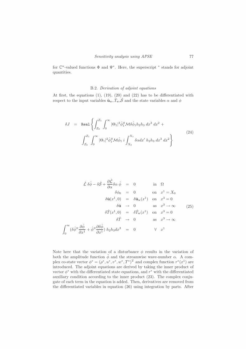
Sensitivity analysis using APSE 77
for Cn-valued functions # and '$. Here, the superscript $ stands for adjointquantities.
B.2. Derivation of adjoint equations
At first, the equations (1), (19), (20) and (22) has to be di!erentiated withrespect to the input variables uw, Tw,S and the state variables ( and 5
0J = Real
2* Z1
Z0
* #
0|$1|25H
1M051h2h3 dx3 dx2 +
* Z1
Z0
* #
0|$1|25H
1M51 i
* X1
X0
0(dx! h2h3 dx3 dx2
5 (24)
L 05# 0S +!L!(
0( 5 = 0 in &
050 = 0 on x1 = X0
0u(x1, 0) = 0uw(x1) on x3 = 0
0u % 0 as x3 %&0T (x1, 0) = 0Tw(x1) on x3 = 0
0T % 0 as x3 %&* #
0(05H !5
!x1+ 5H !05
!x1) h2h3dx3 = 0 0 x1
(25)
Note here that the variation of a disturbance 5 results in the variation ofboth the amplitude function 5 and the streamwise wave-number (. A com-plex co-state vector 5$ = ("$, u$, v$, w$, T $)T and complex function r$(x1) areintroduced. The adjoint equations are derived by taking the inner product ofvector 5$ with the di!erentiated state equations, and r$ with the di!erentiatedauxiliary condition according to the inner product (23). The complex conju-gate of each term in the equation is added. Then, derivatives are removed fromthe di!erentiated variables in equation (26) using integration by parts. After

78 J.O. Pralits, C. Airiau, A. Hanifi & D.S. Henningson
integrations, it yields (without complex conjugate for clarity)
(5$, L 05# 0S +!L!(
0( 5) +* X1
X0
* Z1
Z0
r$* +#
0[05HD1(5) + 5HD1(05)] h1h2h3dx3 dx2 dx1 =
(L$5$, 05)# (5$, 0S)#* X1
X0
* Z1
Z0
* +#
0
!
!x1(5$H !L
!(5 h1h2h3)
* x1
X0
0(dx! dx3 dx2 dx1 +
* Z1
Z0
* +#
0
!5$H !L
!(5 h1h2h3
* x1
X0
0(dx!"X1
X0
dx3 dx2 +
* Z1
Z0
* +#
0
!5$H D 05 h2h3
"X1
X0dx3 dx2 +
* Z1
Z0
* X1
X0
!(5$H
&B # (m13 + m23 #m33) C # D3(C)
'05 +
#D3(5$H) C 05 + 5$H C D3(05))
h1h2 dx2 dx1"#0
+* X1
X0
* Z1
Z0
* +#
0
&r$D1(5H)#D1(r$5H)#
(m21 + m31)r$5H'05 h1h2h3dx3 dx2 dx1 +
* Z1
Z0
* +#
0
!h2h3r
$5H05"X1
X0dx3 dx2 = 0 (26)
where
mij =1
hihj
!hi
!xj.
Terms of 0( have also been integrated in equation (26) in order to identifyfrom 0J the boundary terms at X1. Collecting terms of 05 leads to the adjointequations
L$5$ = #!r$D1(5)#D1(r$5)# (m21 + m31) r$5
"(27)
In order to remove the terms of 05 in the equation (26) as x3 % &, thefollowing homogeneous boundary conditions are chosen
u$(x1, 0) = 0 and T $(x1, 0) = 0,lim
x3%#u$ = 0 and lim
x3%#T $ = 0, (28)
where u$ = (u$, v$, w$)T. Using the operator matrices of the forward problem,the adjoint operator L$ can be identified
L$ = A + B D3. + C D33. + D D1. (29)
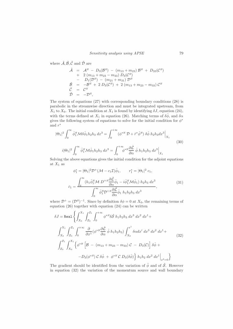
Sensitivity analysis using APSE 79
where A, B, C and D are
A = AH # D3(BH) # (m13 + m23) BH + D33(CH)+ 2 (m13 + m23 #m33) D3(CH)# D1(DH) # (m21 + m31) DH
B = #BH + 2 D3(CH) + 2 (m13 + m23 #m33) CH
C = CH
D = #DH,
The system of equations (27) with corresponding boundary conditions (28) isparabolic in the streamwise direction and must be integrated upstream, fromX1 to X0. The initial condition at X1 is found by identifying 0J , equation (24),with the terms defined at X1 in equation (26). Matching terms of 05, and 0(gives the following system of equations to solve for the initial condition for 5$and r$
|$1|2* #
05H
1M051h2h3 dx3 =* +#
0(5$H D + r$5H) 05 h2h3dx3
111X1
i|$1|2* #
05H
1M51h2h3 dx3 =* +#
05$H !L
!(5 h1h2h3 dx3
111X1
(30)
Solving the above equations gives the initial condition for the adjoint equationsat X1 as
5$1 = |$1|2D+(M# c1I)51, r$1 = |$1|2 c1,
c1 =
* #
0(h15
H1M D+H !L
!(51 # i5H
1M51) h2h3 dx3
* #
05H
1D+H !L!(
51 h1h2h3 dx3
,(31)
where D+ = (DH)"1. Since by definition 05 = 0 at X0, the remaining terms ofequation (26) together with equation (24) can be written
0J = Real
2* X1
X0
* Z1
Z0
* +#
05$H0S h1h2h3 dx3 dx2 dx1+
* X1
X0
* Z1
Z0
* +#
0
!
!x1(5$H !L
!(5 h1h2h3)
* x1
X0
0(dx! dx3 dx2 dx1+
* Z1
Z0
* X1
X0
(5$H
!B # (m13 + m23 #m33) C # D3(C)
"05 +
#D3(5$H) C 05 + 5$H C D3(05))
h1h2 dx2 dx1111x3=0
)
(32)
The gradient should be identified from the variation of 5 and of S. Howeverin equation (32) the variation of the momentum source and wall boundary

80 J.O. Pralits, C. Airiau, A. Hanifi & D.S. Henningson
condition is expressed in terms of 5 and S. The total variation of 5 and S iswritten
05 = 05 $ + 5 i
* x1
X0
0(dx! , 0S = 0S $ + S i
* x1
X0
0(dx! (33)
From equation (33), 05 and 0S are substituted into equation (32). The varia-tion of the functional 0J with respect to the total variation of 5 and S is nowwritten
0J = Real
2* X1
X0
* Z1
Z0
* +#
0
1$5$H0S h1h2h3 dx3 dx2 dx1+
* X1
X0
* Z1
Z0
h1h2
!# $
$ PrRD3(T $)0T +
(""$)$
0w+
µ
$RD3(u$)0u +
µ
$RD3(v$)0v
"dx2 dx1
111x3=0#
* X1
X0
* Z1
Z0
* +#
0
!
!x1(5$H !L
!(5 h1h2h3)
* x1
X0
0(dx! dx3 dx2 dx1+
* X1
X0
* Z1
Z0
* +#
05$HS h1h2h3 i
* x1
X0
0(dx!dx3 dx2 dx1+
* X1
X0
* Z1
Z0
h1h2
!# $
PrRD3(T $)T + (""$)w +
µ
RD3(u$)u+
µ
RD3(v$)v
"i
* x1
X0
0(dx! dx2 dx1111x3=0
5
(34)
In equation (34) the expression for the wall boundary terms have been expandedto clarify the dependence between each state variable and the adjoint quantities.In the derivation of the adjoint equations the co-state variable r$(x) has beenused in order to incorporate the auxiliary condition. However, equation (27)gives a system with five equations and six co-state variables. Therefore, anadditional equation is needed to close the system. Collecting the terms of 0(in equation (34) provides an additional equation which must be satisfied foreach position in x1
* +#
0
!
!x1(5$H !L
!(5 h1h2h3) dx3 = i
* +#
05$HS h1h2h3 dx3+
i h1h2
!# $
PrRD3(T $)T + (""$)w +
µ
RD3(u$)u +
µ
RD3(v$)v
"111x3=0
(35)
It is denoted ’adjoint auxiliary condition’ and is solved with an iterative pro-cess for r$ in a similar manner that equation (22) is solved for the streamwisewavenumber (. The gradient of the functional "J , with respect to the momen-tum forcing and wall disturbances can now be identified from the remaining

Sensitivity analysis using APSE 81
terms of equation (34) as
"uwJ =µ
$RD3(u$) on x3 = 0
"vwJ =µ
$RD3(v$) on x3 = 0
"wwJ =""$
$on x3 = 0
"TwJ = # $
$PrRD3(T $) on x3 = 0
"SJ =5$
$in &
(36)
Appendix C. Operator matricesThe non-zero components of matrices A,B, C and D in equation (21) are
a(1, 1) = U(m31 + m21) + D3(W ) + D1(U) + i,
a(1, 2) = "(i(0 + m31 + m21) + D1(")a(1, 3) = i)0"
a(1, 4) = "(m13 + m23) + D3(")
a(2, 1) =1
%M2(D1(T ) + i(0T ) + D1(U)U + D3(U)W #m21V
2
a(2, 2) = "(D1(U) + i,) +µ
R((2
0l2 + )20)
a(2, 3) = #2"m21V +µ
R(0)0l1
a(2, 4) = "(m13U + D3(U))# i(0
R
dµ
dTD3(T )
a(2, 5) =1
%M2(D1(") + i"(0) +
1R
(# dµ
dTD33(U)#D3(U)
d2µ
dT 2D3(T ))
a(3, 1) = U(m21V + D1(V )) + D3(V )W +i)0
%M2T
a(3, 2) = "(m21V + D1(V )) +µ
R(0)0l1
a(3, 3) = "(m21U + i,) +µ
R()2
0 l2 + (20)
a(3, 4) = "(m23V + D3(V ))# i)0
R
dµ
dTD3(T )
a(3, 5) =i)0
%M2"+
1R
(# dµ
dTD33(V )#D3(V )
d2µ
dT 2D3(T ))
a(4, 1) =1
%M2D3(T )#m13U
2 #m23V2 +
iµ
R
l2"
()0D3(V ) + (0D3(U))

82 J.O. Pralits, C. Airiau, A. Hanifi & D.S. Henningson
a(4, 2) = #2"m13U #i(0
Rl0
dµ
dTD3(T ) +
D3(")"
i(0
Rµl2
a(4, 3) = #2"m23V #i)0
Rl0
dµ
dTD3(T ) +
D3(")"
i)0
Rµl2
a(4, 4) = "(D3(W ) + m31U + i,) +1R
µ()20 + (2
0) +D33(")"
µ
Rl2
a(4, 5) =1
%M2D3(") +
1R
dµ
dTi(#)0D3(V )#D3(U)(0)
a(5, 1) =(% # 1)%
(UD1(T ) + WD3(T ) + iT ,) + cp(#WD3(T )# UD1(T ))
a(5, 2) = (% # 1)M2D1(p)# "cpD1(T )
a(5, 4) = (% # 1)M2
/D3(p) +
2iµ
R()0D3(V ) + D3(U)(0)
0# "cpD3(T )
a(5, 5) = "
6dcp
dT(#WD3(T )# UD1(T )) + i
/(% # 1)%
# cp
0,
7+
1R Pr
/d$
dTD33(T ) +
d2$
dT 2(D3(T ))2 + $(#)2
0 # (20)0
+
(% # 1)R
dµ
dTM2
8(D3(U))2 + (D3(V ))2
9+
(% # 1)%
(UD1(") + WD3("))
b(1, 1) = W
b(1, 4) = "
b(2, 2) = "W # 1R
dµ
dTD3(T )
b(2, 4) = # iµ
R(0l1
b(2, 5) = # 1R
D3(U)dµ
dT
b(3, 3) = "W # 1R
dµ
dTD3(T )
b(3, 4) = # iµ
R)0l1
b(3, 5) = # 1R
D3(V )dµ
dT
b(4, 1) =1
%M2T +
iµ
R
l2",
b(4, 2) =iµ
R(0
b(4, 3) =iµ
R)0

Sensitivity analysis using APSE 83
b(4, 4) = "W +l2R
(2µD3(")"# dµ
dTD3(T ))
b(4, 5) =1
%M2"
b(5, 1) =(% # 1)%
WT
b(5, 2) = 2(% # 1)M2 µ
RD3(U)
b(5, 3) = 2(% # 1)M2 µ
RD3(V )
b(5, 5) = "W
/(% # 1)%
# cp
0+
2R Pr
d$
dTD3(T )
c(2, 2) = # µ
R
c(3, 3) = # µ
R
c(5, 5) =$
R Prd(1, 1) = U
d(1, 2) = "
d(2, 1) =T
%M2
d(2, 2) = "U
d(2, 5) ="
%M2
d(3, 3) = "U
d(4, 4) = "U
d(5, 1) =(% # 1)%
UT
d(5, 5) = "U
/(% # 1)%
# cp
0
where
Di =1hi
!
!xi, Dij =
1hihj
!2
!xi!xj, (0 =
(
h1, )0 =
)
h2, lj =
#
µ+ j,
and, = ((0U + )0V # *).
References
Airiau, C. 2000. ’Non-parallel acoustic receptivity of a Blasius boundary layer usingan adjoint approach.’ to appear in Flow, Turbulence and Combustion.

84 J.O. Pralits, C. Airiau, A. Hanifi & D.S. Henningson
Airiau, C., Walther, S., Bottaro, A. 1999. ’Non-parallel receptivity and theadjoint PSE.’ to appear in IUTAM Symposium on Laminar-Turbulent Transition(September 1999, Sedona, AZ), Fasel, H. and Saric, W., eds. Springer.
Andersson, P., Berggren, M. and Henningson, D.S. 1999. ’Optimal disturban-ces and bypass transition in boundary layer.’ Phys. Fluids, 11, pp. 134–150.
Andersson, P., Henningson, D.S. and Hanifi, A. 1998. ’On a stabilization pro-cedure for the parabolic stability equations.’ J. Eng. Math., 33, pp. 311–332.
Bewley, T.R., Temam, R. and Ziane, M. 2000. ’A general framework for robustcontrol in fluid mechanics.’ Physica D, 138, pp. 360–392.
Bertolotti, F.P., Herbert, Th. and Spalart, S.P. 1992. ’Linear and NonlinearStability of the Blasius Boundary Layer.’ J. Fluid Mech., 242, pp. 441–474.
Cathalifaud, P. and Luchini, P. 2000. ’Algebraic growth in a boundary layer:optimal control by blowing and suction at the wall.’ Eur. J. Mech. B/Fluids,19(4), pp. 469–490
Choudhari, M. and Street, C.L. 1992. ’A finite reynolds-number approach for theprediction of boundary-layer receptivity in localized regions.’ Phys. Fluids A, 4,pp. 2495–2514.
Corke, T.C., Bar-Sever, A. and Morkovin, M.V. 1986. ’Experiments on tran-sition enhancement by distributed roughness.’ Phys. Fluids. 29, pp. 3199–3213.
Crouch, J.D. 1992a. ’Localized receptivity of boundary layers.’ Phys. Fluids A 4,pp. 1408–1414.
Crouch, J.D. 1992b. ’Non-localized receptivity of boundary layers.’ J. Fluid Mech.244, pp. 567–581.
Goldstein, M.E. 1983. ’The evolution of Tollmien-Schlichting waves near the leadingedge.’ J. Fluid Mech. 127, pp. 59–81.
Goldstein, M.E. and Hultgren, L.S. 1989. ’Boundary-layer receptivity to long-wavefree-stream disturbances.’ Ann. Rev. Fluid Mech., 21, pp. 137–166.
Gunzburger, M. 2000. ’Adjoint equation-based methods for control problems inincompressible, viscous flows.’ in press in Flow, Turbulence and Combustion.
Hall, M. C. G. 1986. ’Application of Adjoint Sensitivity Theory to an AtmosphericGeneral Circulation Model.’ J. The Atmospheric Sci. 43, pp. 2644–2651.
Hanifi, A., Henningson, D.s., Hein, S., Bertolotti, F.P. and Simen, M. 1994.’Linear Non-local Instability Analysis - the linear NOLOT code.’ FFA TN 1994-54, See also Hein et al. 1994.
Hanifi, A. and Schmid, P.J., Henningson, D.S. 1996. ’Transient growth in compressibleboundary layer flow’ Phys. Fluids 8(3), pp. 826–837.
Hein, S., Bertolotti, F.P., Simen, M., Hanifi, A. and Henningson, D.S. 1994.’Linear Non-local Instability Analysis - the linear NOLOT code.’ DLR-IB 223-94A 43.
Herbert, Th. 1994. ’Parabolized Stability Equations.’ AGARD Report No. 793, pp.4-1–4-34.
Hill, D. C. 1995. ’Adjoint Systems and their role in the Receptivity Problem forBoundary Layers.’ J. Fluid Mech. 292, pp. 183–204.
Hill, D. C. 1997. ’Receptivity in non-parallel boundary layers.’ ASME Fluids Engi-neering Division Summer Meeting, FEDSM ’97, June 22-26, 1997.
Hogberg, M. and Berggren, M. 2000. ’Numerical approaches to optimal control

85
of a model equation for shear flow instabilities. , Submitted to Journal of Flow,Turbulence and Combustion.
Li, F. and Malik, M.R. 1996 ’On the Nature of PSE Approximation.’ Theoreticaland Computational Fluid Dynamics No.8, pp. 253–273.
Luchini, P. and Bottaro, A. 1998 ’Gortler vortices : a backward-in-time approachto the receptivity problem.’ J. Fluid Mech., 363, pp. 1–23.
Luchini, P. 2000 ’Reynolds-number-independent instability of the boundarylayerover a flat surface: optimal perturbations.’ J. Fluid Mech., 404, pp. 289–309.
Mack, L.M. 1984 ’Boundary-layer stability theory.’ AGARD Report No. 709, pp.3-1–3-81.
Nishioka, M. and Morkovin, M.V. 1986. ’Boundary-layer receptivity to unsteadypressure gradients : experiments and overview.’ J. Fluid Mech. 171, pp. 219–261.
Pralits, J.O., Hanifi, A. and Henningson, D.S. 2000. ’Adjoint-based suctionoptimization for 3D boundary layer flows’ FFA TN 2000-58.
Saric, W.S. 1993. ’Physical description of boundary-layer transition : experimentalevidence’ AGARD report 793, pp. 183–204.
Simen, M. 1992. ’Local and Nonlocal Stability Theory of Spatially Varying Flows.’Instability, Transition and Turbulence, Springer Verlag, pp. 181–201
Thomas, A. 1983. ’The control of boundary-layer transition using a wave superposi-tion principle.’ J. Fluid Mech. 137, pp.233–250.
Tumin, A. 1996. ’Receptivity of Pipe Poiseuille Flow.’ J Fluid Mech. 315, pp. 119–137.


Paper 2 2


Adjoint-based optimization of steady suctionfor disturbance control in incompressible flows
By Jan O. Pralits1,2, Ardeshir Hanifi2,and Dan S. Henningson1,2
The optimal distribution of steady suction needed to control the growth of sin-gle or multiple disturbances in quasi three-dimensional incompressible bound-ary layers on a flat plate is investigated. The evolution of disturbances isanalyzed in the framework of the Parabolized Stability Equations (PSE). Agradient based optimization procedure is used and the gradients are evaluatedusing the adjoint of the parabolized stability equations (APSE) and the ad-joint of the boundary layer equations (ABLE). The accuracy of the gradient isincreased by introducing a stabilization procedure for the PSE. Results showthat a suction peak appears in the upstream part of the suction region for opti-mal control of Tollmien-Schlichting (T-S) waves, steady streamwise streaks in atwo-dimensional boundary layer and oblique waves in a quasi three-dimensionalboundary layer subject to an adverse pressure gradient. The mean flow modi-fications due to suction are shown to have a stabilizing e!ect similar to that ofa favorable pressure gradient. It is also shown that the optimal suction distri-bution for the disturbance of interest reduce the growth rate of other pertur-bations. Results for control of a steady cross-flow mode in a three-dimensionalboundary layer subject to a favorable pressure gradient show that not evenlarge amounts of suction manages to completely stabilize the disturbance.
1. IntroductionLaminar-turbulent transition in boundary layers on aircrafts causes a rapid in-crease of the skin friction and consequently a larger drag. Therefore, delay oftransition occurrence will reduce the fuel consumption which results in a loweroperation cost and less pollution. Transition in the boundary layer on aircraftwings is usually caused by break down of small disturbances which grow as theypropagate down stream. It is well known that growth of such disturbances canbe suppressed or controlled by steady- or unsteady wall-suction. The latteris sometimes referred to as the wave-cancellation concept and has been inves-tigated both numerically and experimentally by numerous authors, see Joslin(1998) for an excellent overview of earlier experimental and numerical works.
1Department of Mechanics, KTH, SE-100 44 Stockholm, Sweden.2Swedish Defence Research Agency, FOI, Aeronautics Division, FFA, SE-172 90 Stockholm,Sweden.
89

90 J. O. Pralits, A. Hanifi & D. S. Henningson
Steady suction implies that a modification of the steady mean flow is done.Here, the aim is to reduce the thickness of the boundary layer and to stabilizethe mean velocity profile. The inviscid instability in two-dimensional boundarylayers, which is related to the second wall-normal derivative of the streamwisevelocity, is stabilized by suction. A similar stabilizing e!ect is obtained byimposing a favorable pressure gradient given zero suction on the wall. Therelation between suction, the pressure gradient and the viscous terms in two-dimensional boundary layers is well explained in e. g. Schlichting (1979). Themean flow obtained using non-zero suction have similarities with those obtainedwhen a negative pressure gradient is applied. In the case of an adverse pressuregradient present in the flow, the superposition of suction will reduce the cur-vature of the velocity profile at the wall, weakening the inflection in the profilewhich inhibits the inviscid instability. It should be noted that the discussionabove relates primarily to exponential instabilities.
Constant steady suction has been studied both experimentally and numer-ically by several authors. Iglisch (1949) investigated theoretically the initiallength needed for the shape factor (displacement thickness/momentum thick-ness) to reach a constant value in the case of a flat plate two-dimensional bound-ary layer. Here, the streamwise velocity profile becomes ’fuller’ downstream assuction is applied finally reaching the so called ’asymptotic suction profile’.With the assumption of an asymptotic velocity profile present along the wholeplate, the laminar boundary layer is stable with respect to two-dimensional T-Swave instabilities if the constant suction velocity Vw = V !
w/U!# = 1.4 ( 10"5.
Here, V !w and U!
# are the dimensional wall-normal suction velocity at the walland free-stream velocity components of the mean flow, respectively. For thesame case, Ulrich (1944) showed that the critical Reynolds number, Recrit, infact decreases as one approaches the leading edge. Hence, an increasing amountof suction is required in this region. In Schlichting (1979) it was shown that acorrection due to increased amount of suction close to the leading edge leads toa constant suction velocity Vw = 1.2(10"4 in order to maintain a laminar flowalong the whole plate. The increased suction velocity due to the correction ofthe initial length is an increased amount of suction energy. If a large amountof suction is applied then the power saved by the reduction in drag might wellbe lost by the power used for the suction device. Further, if a large amountof suction is used, resulting in a thinning of the boundary layer then this maylead to an increase of the shear stress at the wall. It is therefore of interest toinvestigate if a more optimal suction distribution can be obtained which meetsthe objective of reducing the disturbances present in the flow while using theleast amount of suction energy.
In the last decade more interest has been focused on optimal control of fluidflows in which optimal control theory has been utilized in di!erent manners.Here, the objective is to minimize some measure of the state with a prescribedamount of suction on the wall. This can mathematically be described by aminimization of an objective function which balances a measure of the state

Optimization of steady suction for disturbance control 91
and a measure of the control. The problem can be solved using the sensitivityinformation given by the gradient of the objective function with respect to thecontrol in a gradient based optimization routine. An e"cient way to calculatethe gradients is the adjoint approach which has been shown successful in nu-merous applications such as shape optimization, optimal control, receptivity,meteorology and optimal perturbations as long as the number of constraintsare low and the control-variable space is large. A recent workshop on adjointsystems, see Flow, Turbulence and Combustion 2000 Vol. 65 (3/4), indicatesome of the progress in the field.
Here the wall-normal velocity component of the steady mean flow on thewall is used as the control, which means that the suction will modify the meanflow to control disturbance growth rather than generating an out-of phase dis-turbance by time periodic suction. Another investigation was done by Balaku-mar & Hall (1999) who used a Lagrangian approach to find the optimal suctiondistribution for Blasius and swept Hiemenz flows. The objective was to movethe transition point, given by the eN -method, downstream. They found thatfor Blasius boundary layers the optimal suction distribution peaked upstreamof the maximum growth rate and decreases to zero at the transition point.
In the present work we use an approach di!erent from that in Balakumar& Hall (1999). The control problem is defined using optimal control theoryin which a gradient-based technique is used to update the control during theoptimization process. The aim is to minimize a given objective function bal-ancing a measure of the total disturbance kinetic energy and the control energy.The mean flow is found by solving the quasi three-dimensional boundary layerequations for incompressible flows and the growth of disturbances is analyzedfor developing boundary layers using the PSE (see Bertolotti et al. 1992; Malik& Balakumar 1992; Simen 1992; Herbert 1997). In the frame work of thesegoverning equations we can analyze convective instabilities under the assump-tion of a slow variation of both the mean flow and the shape function of thedisturbances in the streamwise direction. We also assume that the streamwisepressure distribution is not a!ected by suction at the wall. The mean flowis obtained using the boundary layer equations (see eg. Schlichting 1979). Inthis approximation, as well as in higher order approximations, the wall normalvelocity of the mean flow, V, is of order O(1/Re). Here Re = U!
#l!/&! is theReynolds number in which l! and &! denotes the dimensional reference lengthand kinematic viscosity, respectively. In the optimization one must make surethat this assumption is not violated.
An adjoint-based technique is used to evaluate the gradients (sensitivities).Here, we couple the adjoint of the PSE with the adjoint of the boundary-layer equations in order to find the gradient of the disturbance growth dueto modifications of the mean flow. The use of the adjoint PSE (APSE) wasfirst proposed by Herbert (1997) and has then been used for receptivity studies(see Hill 1997a; Airiau 2000; Dobrinsky & Collis 2000), sensitivity analysis(see Pralits et al. 2000) and optimal control problems (see Hill 1997b; Pralits

92 J. O. Pralits, A. Hanifi & D. S. Henningson
et al. 2000b; Walther et al. 2001). Hill (1997b) used a similar approach ininverse design for laminar boundary layer. However, no details were given there.The common interest of all these applications lies in the e"cient evaluation ofreceptivity-coe"cients and sensitivity information provided by a single solutionof the APSE. The major di!erence between previous works is found in thederivation of the APSE. In Hill (1997a,b); Airiau (2000); Dobrinsky & Collis(2000) the APSE is an approximation of the adjoint of the linearized Navier–Stokes equations given an ansatz similar to the PSE. The additional equationused to find the “adjoint” streamwise wave number comes from an orthogonalityrelation between the solutions from the APSE and PSE. In Dobrinsky & Collis(2000) it is shown that this condition in fact does not hold in a large partof the domain which means a less accurate result of the adjoint equations.The reason is said to depend on the numerical scheme and approximate inflowconditions. In Pralits et al. (2000) the APSE is derived directly from the PSEusing a variational technique and the additional equation and inflow conditionsare part of the definition of the adjoint operator. The latter technique, whichis shown to have good accuracy in the major part of the domain, is also usedin Pralits et al. (2000b) and Walther et al. (2001).
The optimization process is dependent on the accuracy of the gradient(search-direction), which can be evaluated to better assess the optimizationresults. In the present work, the gradient is derived from the continuous stateequations which means that its accuracy can be improved if the resolution isincreased, see e. g. Hogberg & Berggren (2000). However, the PSE is knownfor its instability for small streamwise steps due to the remaining ellipticity.Several studies on how to stabilize the PSE have been done (see Haj-Hariri1994; Li & Malik 1994, 1996; Andersson et al. 1998). The approach which bestremoves the ellipticity while still producing an accurate result is the techniqueintroduced by Andersson et al. (1998), where originally neglected higher orderterms, O(Re"2), are reintroduced. This stabilization procedure will also a!ectthe adjoint equations (see § 2.4).
In this paper we present a method which involves solving a number ofproblems regarding the derivation of the gradient, adjoint equations and sta-bilization of the adjoint equations. For this reason, a large part of the paperis dedicated to explaining the di!erent steps in detail. The optimal controlproblem and the corresponding equations are presented in § 2. In § 3, a valida-tion of the adjoint equations is done by analyzing the gradient accuracy. Herewe also show results on optimal control of steady streamwise streaks and T-Swaves in a two-dimensional boundary layer, and oblique waves and a steadycross-flow mode in a quasi three-dimensional boundary layer. The discussionand concluding remarks are given in § 4 and the complete derivation of the gra-dient and the coupling of the adjoint of the parabolized stability and boundarylayer equations are shown in Appendix B. A preliminary version of the workpresented here can be found in the report by Pralits et al. (2000b).

Optimization of steady suction for disturbance control 93
2. Problem formulationThis section presents the optimal control problem for incompressible flows. Forsimplicity, we restrict our analysis to a plane geometry.
2.1. State equations
The flow field is given by the solution of the mass and momentum conserva-tion equations for a viscous flow. The equations are written for a Cartesiancoordinate system with streamwise, normal and spanwise coordinates denotedas x, y and z, respectively. The flow field is decomposed into a mean, Q, anda perturbation part, q, as
Qtot(x, y, z, t) = Q(x, y) + q(x, y, z, t)
where Q = (U, V, W, P )T and q = (u, v, w, p)T. The mean flow, which haszero variation in the spanwise direction, is a three-component, two-dimensionalboundary layer and is here referred to as a quasi three-dimensional boundarylayer. The evolution of disturbances is analyzed in the framework of the nonlo-cal stability theory (see e. g. Bertolotti et al. 1992; Malik & Balakumar 1992;Simen 1992; Herbert 1997).
In the following sections the equations for the mean flow and disturbances,in non-dimensional form, are given. The velocity components are made non-dimensional by U!
#, the pressure by "!U!2# and the reference length is taken
as l!0 = (&!x!0/U!
#) 12 . Here superscript ! denotes dimensional quantities, &! the
kinematic viscosity, U!# the free stream velocity and "! the density.
2.1.1. Mean flow equations
The non-dimensional boundary layer equations for a quasi three-dimensionalincompressible flow on a flat plate with an external pressure gradient given asdPe/dx = #UedUe/dx can be written
!U
!x+!V
!y= 0, (1)
U!U
!x+ V
!U
!y# Ue
dUe
dx# 1
Re
!2U
!y2= 0, (2)
U!W
!x+ V
!W
!y# 1
Re
!2W
!y2= 0, (3)
with the boundary conditions
U = W = 0, V = Vw on y = 0,
(U, W )% (Ue, We) as y %&,(4)
where index e denotes that the variable is evaluated at the boundary layer edgeand Re = l!0U
!#/&! is the Reynolds number. Note that for the boundary layer
approximations to be valid, the normal velocity at the wall, Vw = V !w/U!
#,should be of order O(Re"1).

94 J. O. Pralits, A. Hanifi & D. S. Henningson
2.1.2. Disturbance equations
We assume the perturbations to be time and spanwise periodic disturbances as
q(x, y, z, t) = q(x, y) exp i&* x!
X0
( dx! + )z # *t'
+ c.c., (5)
where ( is the complex streamwise wavenumber, ) the real spanwise wavenum-ber and * the real disturbance angular frequency. We assume a scale separationRe"1 between the weak variation in x-direction and the strong variation in they-direction. It is also assumed that !/!x 4 O(Re"1) and V 4 O(Re"1). In-troducing (5) and the assumptions above in the linearized governing equationsand keeping terms up to order O(Re"1), yield a set of nearly parabolic partialdi!erential equations
Aq + B!q
!y+ C
!2q
!y2+ D
!q
!x= 0, (6)
where the matrices A, B, C and D are given in Appendix A. For a note onthe parabolic nature of the PSE see Bertolotti et al. (1992); Haj-Hariri (1994);Li & Malik (1994, 1996); Andersson et al. (1998). To remove the ambiguityof having x-dependence of both the amplitude function and wave function in(5) and to maintain a slow variation of the amplitude function q, a so called’auxiliary condition’ is introduced
* #
0uH !u
!xdy = 0, (7)
where u = (u, v, w)T and superscript H denotes the complex conjugate trans-pose. The disturbances are subjected to the following boundary conditions
u = 0 on y = 0u% 0 as y %&.
(8)
The system of equations (6) and (7), is integrated in the downstream directionwith the initial condition given by the solution of the local stability theory atx = X0. At each streamwise position, the value of ( is iterated such that (7)is satisfied.
2.2. Optimal control of a single disturbance
In this section, we define an optimal control problem where the mean normalvelocity at the wall is optimized to reduce the growth of a single disturbancewith a fixed given initital condition. The optimization problem is solved byminimizing an objective function balancing a measure of the state and thecontrol using a gradient based method. We obtain the gradient of the objectivefunction using an adjoint technique. The complete derivation of the equationscan be seen in Appendix B.

Optimization of steady suction for disturbance control 95
y
x
z
X0
X1
U
Vw
(c
Q#
U# W#
Pe
Figure 1. Computational domain: flat-plate boundary layer
2.2.1. Objective function
We measure the size of a disturbance in domain &, defined such that x '[X0, X1], y ' [0,&) and z ' [Z0, Z1] (see figure 1), by its total kinetic energydefined as
E =12
* Z1
Z0
* X1
X0
* #
0uTu dy dx dz.
The objective function to be minimized is
J(Vw) =12
* Z1
Z0
* X1
X0
* #
0uTu dy dx dz +
l2
2
* Z1
Z0
* X1
X0
Vw2 dx dz (9)
where l2 > 0, is the regularization parameter and is used to insure that thesize of the control parameter Vw does not grow unbounded. Now, the controlproblem can be defined mathematically as
find V optw ' L2((c) such that
J(V optw ) + J(Vw) 0 Vw ' L2((c)
(10)
where V optw is the optimal suction distribution on the wall.
2.2.2. Adjoint equations and the gradient
The gradient of the objective function (9) with respect to the control variableis defined through the directional derivative as
0J = -"VwJ, 0Vw. = lims%0
1111J(Vw + s0Vw)# J(Vw)
s
1111 , (11)
where 0Vw is the variation of the control variable. Here, we derive the gradientexpression using the adjoint of the state equations. Details of the derivation isgiven in Appendix B. This yields
"VwJ = l2Vw + V $w on y = 0. (12)
The value of V $w = V $(x, 0) in (12) is given by the solution of the adjoint of the
PSE and boundary layer equations, hereafter referred to as APSE and ABLE,
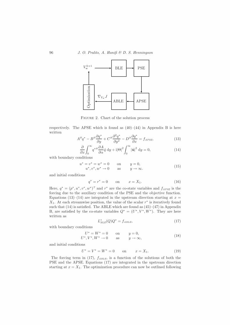
96 J. O. Pralits, A. Hanifi & D. S. Henningson
V k+1w
"VwJ
BLE PSE
ABLE APSE
Opt
imiz
atio
n
Figure 2. Chart of the solution process
respectively. The APSE which is found as (40)–(44) in Appendix B is herewritten
AHq$ #BH !q$
!y+ CH !
2q$
!y2#DH !q$
!x= fAPSE, (13)
!
!x
* #
0q$H !A
!(q dy + i|$|2
* #
0|u|2 dy = 0, (14)
with boundary conditions
u$ = v$ = w$ = 0 on y = 0,u$, v$, w$ % 0 as y %&.
(15)
and initial conditions
q$ = r$ = 0 on x = X1. (16)
Here, q$ = (p$, u$, v$, w$)T and r$ are the co-state variables and fAPSE is theforcing due to the auxiliary condition of the PSE and the objective function.Equations (13)–(14) are integrated in the upstream direction starting at x =X1. At each streamwise position, the value of the scalar r$ is iteratively foundsuch that (14) is satisfied. The ABLE which are found as (45)–(47) in AppendixB, are satisfied by the co-state variables Q$ = (U$, V $, W $). They are herewritten as
L$BLE(Q)Q$ = fABLE, (17)
with boundary conditions
U$ = W $ = 0 on y = 0,U$, V $, W $ % 0 as y %&,
(18)
and initial conditions
U$ = V $ = W $ = 0 on x = X1. (19)
The forcing term in (17), fABLE, is a function of the solutions of both thePSE and the APSE. Equations (17) are integrated in the upstream directionstarting at x = X1. The optimization procedure can now be outlined following

Optimization of steady suction for disturbance control 97
the steps below considering the chart given in figure 2 where k denotes theiteration number.
i. The BLE (1)–(3) are integrated from x = X0 to x = X1. If k = 1 thenV k
w = 0 (initial guess on the suction distribution).ii. The PSE (6)–(7) are integrated from x = X0 to x = X1, then the APSE
are integrated from x = X1 to x = X0.iii. fABLE is calculated from the solution of both the PSE and APSE.iv. The ABLE (17) are integrated from x = X1 to x = X0 given the forcing,
fABLE, from (iii).v. If k < 2 then goto (vi), else evaluate the convergence criteria: If Jk+1#
Jk < err then convergence is reached else goto (vi). Here err is a smallreal-valued parameter defining the convergence.
vi. The gradient, (12), is evaluated and the new boundary condition for theBLE, V k+1
w , is calculated using an optimization routine (here we use alimited-memory quasi-Newton method). Continue: k = k+1, goto (i).
The gradient of the objective function due to a variation of the free streamvelocity can be derived in the same manner as for Vw and yields,
"UeJ = #Ue
* #
0
!U$
!xdy. (20)
This variation would be the result of a change in the geometry and consequentlythe pressure distribution. E!ects due to geometry changes are not investigatedhere.
2.3. Optimal control of multiple disturbances
In this section we generalize the technique introduced above to find the optimalsuction distribution of the steady mean flow that accounts for the growth ofmore than one disturbance. This is necessary for cases where it is not possibleto clearly state which disturbance will grow the most and thus cause laminar-turbulent transition first. An example of this is the two-dimensional Blasiusboundary layer where either T-S wave type instabilities or steady streamwisestreaks could give the maximum growth at a given streamwise position. Themeasure of disturbance kinetic energy in &, is now taken as the sum of theenergy of a chosen number of pre-defined disturbances in a convectively un-stable flow. In this case, the suction distribution will be optimal for the sumof these disturbances. Our approach is however di!erent from non-cooperativestrategies (see Bewley & Liu 1998; Bewley & Moin 1997) which analyze worst-case scenarios, so called robust control. There, the strategy is to find the bestcontrol in the presence of the worst case external disturbance.
The analysis does not di!er much from the one outlined in § 2.2 and istherefore done here on a more compact form. If we denote the total number of
98 J. O. Pralits, A. Hanifi & D. S. Henningson
existing disturbances with N then the total kinetic energy is defined as
E =N%
k=1
12
* Z1
Z0
* X1
X0
* #
0uk
Tuk dy dx dz.
The objective function to be minimized is now
J(Vw) =N%
k=1
12
* Z1
Z0
* X1
X0
* #
0uk
Tuk dy dx dz +l2
2
* Z1
Z0
* X1
X0
Vw2 dx dz. (21)
The same procedure to find the gradient of J with respect to Vw given in Ap-pendix B for control of single disturbances is now used to account for severaldisturbances. As the control problem is derived for steady suction, the case ofmultiple disturbances does not introduce any further complications. Equation(11) is used to define the gradient which can now be written
"VwJ = l2Vw +N%
k=1
(V $w)k on y = 0. (22)
Equation (22) implies that each equation in the solution procedure given infigure 2 must be solved N times, i. e. for each disturbance, before evaluatingthe gradient. Instead, one can use the fact that the ABLE are linear equations.In this case, for a given solution of the BLE, the PSE and the APSE aresolved N times, step (ii) in figure 2. The forcing term of the ABLE, step (iii),is then computed as the sum of N realizations. In step (iv), the ABLE aresolved once given the total forcing from all N disturbances. The gradient isfinally evaluated from (12) which was given for control of single disturbances.However, now a single evaluation of V $
w accounts for all N disturbances.It should be mentioned that the evaluation of the initial disturbances far
upstream of the neutral point may be di"cult. Therefore, if we consider a largenumber of di!erent disturbances whose neutral points are widely spread in thestreamwise direction, care has to be taken when X0 is chosen.
2.4. Adjoint of the stabilized PSE
In gradient based optimization, an increased accuracy of the gradient will givea result closer to the optimum. The gradient presented here, (12), is derivedusing a so called continuous approach. This means that the adjoint of a stateequation is derived from the continuous equation and then discretized. Anotherapproach is to first discretize the state equation and then derive its adjoint,the so called discrete approach. The latter yields a more accurate gradientin most cases but its derivation is more complicated. However, results of thecontinuous approach should converge to that of the discrete one as the gridresolution is refined, (see Hogberg & Berggren 2000). It is a rather well knowproblem that the PSE equations become unstable as the grid in the streamwisedirection is refined due to a remaining ellipticity in the equations, (see Haj-Hariri 1994; Li & Malik 1994, 1996; Andersson et al. 1998). This problem willtherefore put a limit on the accuracy of the gradient unless some technique is

Optimization of steady suction for disturbance control 99
used to overcome the instability problem and allow a smaller step-size in thestreamwise direction. A stabilization procedure was presented by Anderssonet al. (1998) in which they add terms proportional to the truncation error of theimplicit scheme used in the streamwise direction. These terms are of the sameorder as some of the originally neglected terms in the PSE. It was shown thatthe procedure does not alter the PSE results while allowing higher streamwiseresolution. The procedure here, does however not only add terms to the PSEbut also a!ects all adjoint equations since we derive the adjoint from the PSEand not the adjoint linearized Navier–Stokes equations. Here, we present theoutline on how to derive the PSE, gradient and the adjoint equations, using thestabilization technique given by Andersson et al.. The details of the derivationcan be seen in B.3. Following Andersson et al., terms of order O(Re"2) areintroduced in (6). The stabilized PSE can be written
#D!q
!x= A
!q + s
!q
!x
"+ B
!!q
!y+ s
!
!x
&!q
!y
'"+
C!!2q
!y2+ s
!
!x
&!2q
!y2
'"(23)
where s is a positive real number. The gradient, (12) and the adjoint equationswere derived in Appendix B without the stabilization terms. Now, the deriva-tion has to be done using (23) instead of (6) which yields the following adjointequations
#DH !q$
!x= #
!AHq$ # sAH !q$
!x
"+ BH
!!q$
!y# s
!
!x
&!q$
!y
'"#
CH!!2q$
!y2# s
!
!x
&!2q$
!y2
'"+ fAPSE (24)
!
!x
* #
0q$H !A
!(
!q + s
!q
!x
"dy + i|$|2
* #
0|u|2 dy = 0, (25)
L$BLE(Q)Q$ = fABLE, (26)
where fAPSE and fABLE denotes the forcing terms of the APSE and ABLErespectively and the accent˜marks where additional terms due to the stabiliza-tion procedure appear. Note here, that there is no influence on the gradientexpression or on the boundary conditions of the state and adjoint equations dueto the stabilizing terms. The additional terms on the right hand side of (24)resembles the stabilizing terms in (23) apart from the sign di!erence on s. TheAPSE resembles the PSE and the new right hand side of (24) will indeed workas a stabilizing term allowing a smaller step-size in the streamwise directionand the calculation of a more accurate gradient.
3. ResultsThe results presented are obtained by numerically integrating the discretizedstate and co-state (adjoint) equations. The x-derivatives are approximated bya first- or second-order accurate backward Euler scheme. The y-derivatives of

100 J. O. Pralits, A. Hanifi & D. S. Henningson
the PSE and APSE are approximated by Chebychev-polynomials and a second-order accurate finite-di!erence scheme for the BLE and ABLE. The L-BFGS-Bpackage, which is based on the limited memory quasi-Newton method, is usedin the optimization procedure (see Zhu et al. 1994; Byrd et al. 1995). Here wetake Jk+1 # Jk = 10"15 as a converged solution. The gradient accuracy hasbeen checked for the first and last iteration of the optimization process.
In all the results shown here, except for figure 9, the optimal suction distri-bution is computed for the whole streamwise computational domain. In figure 9di!erent control domains are investigated. In all computations, the suction iszero at the first streamwise point to assure that the original assumption of zerovariation of disturbance at X0 is met.
The relation between the regularization parameter, reduction of distur-bance kinetic energy and control energy for all cases is found in the end of thissection.
3.1. Validation and accuracy of the gradient
The optimization procedure depends on the accuracy of the gradient. If itsaccuracy is low, then it is less likely to find a minima and convergence prob-lems will be encountered. Here, we check the accuracy of the gradient by acomparison of the adjoint based gradients (12) with those obtained from afinite-di!erence approach. The comparison is done considering a wall normalvelocity perturbation 0Vw at y = 0. The variation of the functional J withrespect to this perturbation is
0J =!J
!Vw0Vw. (27)
In the finite-di!erence approach !J/!Vw is obtained by using the inhomoge-neous wall boundary-condition Vw = ±.w at x = xn. The index n refers tothe n-th streamwise position and .w is a small positive number. The derivativeis then evaluated using a second-order accurate finite-di!erence scheme. Thediscretized expression for 0J in the adjoint approach is given by
0J =* X1
X0
&N"1%
n=2
"VwJn 0Vwn%n
'dx (28)
where %n = (xn+1#xn"1)/2. In figure 3(b), the relative error between dJ/dVw
and "VwJn%n is compared for di!erent streamwise resolution %Re. The cal-culations are done for a streamwise range Re = 250 # 760 on a quasi three-dimensional boundary layer where dPe/dx = 0 given a T-S wave as the initialdisturbance at x = X0. The inviscid flow at Re = 250 has an angle of 30o,the non-dimensional spanwise wavenumber ) = 0 and the reduced frequencyF = 2-f!&!
e /U!e
2 = 10"4. As can be seen in figure 3(b), the relative errordecreases as the %Re is decreased. Here, %Re = 6 is the minimum streamwisestep size for which the PSE calculations are stable. The values for %Re = 2are computed using the stabilization terms, explained in § 2.4. In figure 3(a),

Optimization of steady suction for disturbance control 101
(a) (b)
"VwJ err
200 400 600 800Re0
200
400
600
800
200 400 600 800Re10−4
10−3
10−2
10−1
100
$Re=10$Re=6$Re=2 (stabilized)
Figure 3. Comparison of the gradient from adjoint andcentral-di!erence calculations for di!erent streamwise resolu-tion %Re. (a) %Re = 2, the continuous line is the gradi-ent derived from adjoint equations, • marks central-di!erencecalculations. (b) The relative error (err) between adjointand central-di!erence calculations of the gradient for di!er-ent streamwise resolution %Re.
the gradient obtained from the adjoint equations is compared with central-di!erences when %Re = 2 in order to visualize the agreement.
The results presented in § 3, has a %Re chosen such that the relative error(err) was approximately 1%, which required the use of the stabilization pro-cedure. A study was conducted on the influence of changing the streamwiseresolution for control of T-S waves in the Blasius boundary layer. It was foundthat an increased resolution gives a faster convergence and a decrease of theobjective function.
3.2. Two-dimensional boundary layers
In this section we investigate the disturbance control in a two-dimensionalboundary layer with zero pressure gradient. The disturbances studied here arechosen to be a T-S wave and/or optimally growing steady streamwise streaks.The initial conditions for T-S waves are taken as the solutions of the localstability theory and the initial condition for the streaks has been calculatedusing the theory given in Andersson et al. (1999). For T-S waves, the stream-wise range is chosen such that the unstable region is found between X0 andX1. In § 3.2.1 the optimal suction distribution is calculated to control each ofthese disturbances individually. Here, we also investigate the e!ect of di!erentdomains along the streamwise axis for the control of T-S waves.
The results in this section on control of T-S waves are produced for adisturbance with a frequency of F = 10"4. It is shown that the optimalsuction distribution obtained to control the chosen T-S wave has a stabilizinge!ect on T-S waves with other frequencies. A study has also been performed to

102 J. O. Pralits, A. Hanifi & D. S. Henningson
(a) (b)
(c) (d)
400 500 600 700 800Re
−12
−8
−4
0
VW x 103
400 500 600 700 800Re
−5
−4
−3
−2
−1
0
VW x 102
0 2 4 6 8 10 12iterations
10−1
100
101
102
103
J
400 500 600 700 800Re
10−6
10−4
10−2
100
E
VW=0l2=103
l2=101
l2=1
#1−7
Figure 4. Disturbance control of optimally growing steadystreamwise streaks in a two-dimensional boundary layer(dPe/dx = 0). The non-dimensional spanwise wavenumber) = 0.292 at Re = 412. Results are shown for l2 = 1, 10, 103.(a) Optimal suction distributions. (b) The disturbance ki-netic energy in a mean flow with zero and optimal suctiondistribution. (c) Suction profiles for the di!erent steps in theoptimization process, l2 = 103. (d) The objective function asa function of the iteration step.
control T-S waves with both higher and lower frequencies than the one shownhere. However, the e!ect of the optimization process on the growth rate ofthese disturbances, the corresponding optimal suction profiles and mean flowmodifications all show the same behavior. Thus this choice of frequency givethe general behavior of the optimization process given a T-S wave instabilityin a two-dimensional boundary layer.
3.2.1. Control of single disturbances
The optimal distribution of suction to control steady streamwise streaks is cal-culated for a streamwise range Re = 412 # 730. The initial condition whichhas the maximum energy at X1, is computed using the optimization procedure

Optimization of steady suction for disturbance control 103
(a) (b)
(c) (d)
200 400 600 800Re−0.02
−0.01
0
0.01
grow
th ra
te
200 400 600 800Re−2
−1.5
−1
−0.5
0
VW x 104
VW x 104
VW x 3.103
VW x 103
0 4 8 12iterations
0
0.5
1
2
J
200 400 600 800Re10−7
10−6
10−5
10−4
10−3
10−2
E
VW=0l2=105
l2=104
l2=103
l2=102
Figure 5. Disturbance control of a T-S wave with F = 10"4
in a two-dimensional boundary layer (dPe/dx = 0). Resultsare shown for l2 = 102, 103, 104, 105. (a) Optimal suction dis-tributions (note the di!erent scalings). (b) The disturbancekinetic energy in a mean flow with zero and optimal suctiondistribution. (c) The growth rate, -imag((), in a mean flowwith zero and optimal suction. (d) The objective function asa function of the iteration step.
given in Andersson et al. (1999). The non-dimensional spanwise wavenumber) = 0.292 and the frequency * = 0. Three test cases are analyzed for theseparameters in which the regularization parameter l2 was 1, 10 and 103 andthe control is applied at Re = 418 # 724. In figure 4(a) the optimal suctiondistributions for all cases are compared. A peak in the suction distribution isnoticed upstream which becomes more pronounced as the regularization pa-rameter is decreased. In figure 4(b) the disturbance kinetic energy of zero andoptimal suction are compared. All three suction distributions result in a de-crease of the disturbance kinetic energy. However, the main di!erence betweenthe curves where control is applied is seen in the upstream region. The e!ectof the optimal suction distributions given in figure 4(a) is that the dampingof the disturbance kinetic energy is increased in the upstream region as l2 is

104 J. O. Pralits, A. Hanifi & D. S. Henningson
200 400 600 800Re
−0.002
0
0.002
0.004
0.006
grow
th ra
temax. growth, Vw=0max. growth, l2=105
F=10−4, Vw=0F=10−4, l2=105
Figure 6. Maximum local growth rate compared with localgrowth rate of a T-S wave with F = 10"4, for zero and optimalsuction in a two-dimensional boundary layer (dPe/dx = 0).The optimal suction is computed for control of a T-S wavewith F = 10"4 given that l2 = 105 for a streamwise rangeRe = 250 # 760. Calculations of maximum local growth rateare made with %F = 2.5( 10"6.
decreased. Figure 4(c) illustrates the changes in the suction distribution dur-ing the optimization procedure. Here, Vw is plotted for each iteration in theoptimization loop for the case with l2 = 102. The optimal distribution is foundafter 7 iterations. The di!erence between the sixth and seventh iteration cannot be distinguished. In figure 4(d) the objective function is given as func-tion of the iteration number for all cases to illustrate the convergence of theoptimization procedure.
The optimal distribution of suction to control T-S wave instabilities iscalculated for a streamwise range Re = 250#760. The first investigation is doneby comparing di!erent regularization parameters, here l2 = 102, 103, 104, 105
while control is applied at Re = 256# 754. The results can be seen in figure 5.In figure 5(a) the optimal suction distributions from all cases are compared.Here, it is noted that the optimal suction distribution tends to peak upstreamas the penalty on the control is reduced, and this peak is upstream of theunstable region for all cases. Even though the magnitude of the suction ratesare within the original assumptions, one should also note that a decreasedpenalty on the control produces suction distributions with large streamwisevariations in the upstream domain. At the point where our results show apeak they are thus locally outside the range of validity of the parabolic theoryemployed, since the gradient of the control velocity at the initial control point

Optimization of steady suction for disturbance control 105
(a) (b)
(c) (d)
y!/l!0
y!/l!0
0 0.2 0.4 0.6 0.8 1U
0
5
10
15Re=256, (VW=0)Re=256, (VW=optimal) Re=400, (VW=0)Re=400, (VW=optimal)Re=598, (VW=0)Re=598, (VW=optimal)
0.00 0.01 0.02 0.03u0
5
10
15Re=256, (VW=0)Re=256, (VW=optimal) Re=400, (VW=0)Re=400, X 5 (VW=optimal)Re=598, (VW=0)Re=598, X 30 (VW=optimal)
−0.002 0 0.002 0.004V
0
10
20
30
40
0.000 0.001 0.002 0.003 0.004 0.005v
0
10
20
30
40
Figure 7. Modification of the two-dimensional mean flow(dPe/dx = 0) and disturbance velocity due to optimal suc-tion computed to control a T-S wave with F = 10"4 whenl2 = 102 in a streamwise range Re = 250 # 760. Results arepresented for Re = 256, 400, 598. (a) Streamwise and (c) wallnormal velocity of the mean flow subject to zero and optimalsuction. Absolute value of the (b) streamwise and (d) wallnormal disturbance velocity (note the di!erent scalings).
approaches infinity as the step size in the streamwise direction approacheszero. In figure 5(b) the disturbance kinetic energy is compared for zero andoptimal suction distribution. A reduction of disturbance kinetic energy canbe observed as the penalty of the control is reduced. The growth rate for allcases can are given in figure 5(c). In all cases the growth rate is decreased asl2 is decreased and the reduction is more pronounced in the upstream region.Finally, in figure 5(d) the objective function is plotted as a function of theiteration number to show the convergence of the optimization procedure.
A question that arises is if the suction distribution which is optimal forone chosen T-S wave will damp or amplify other instability waves in the cho-sen streamwise domain. This is analyzed by computing the maximum local

106 J. O. Pralits, A. Hanifi & D. S. Henningson
growth rate, i. e. local growth rate over all possible frequencies, at a numberof streamwise positions both with zero and the optimal suction distribution.The streamwise range and optimal suction distribution are taken from figure 5with l2 = 105. The results are shown in figure 6 where the maximum localgrowth rate has been computed for %F = 2.5 ( 10"6 and %Re = 50 as thereduced frequency and streamwise resolution respectively. Here, it is shownthat the optimal suction distribution for one given frequency has a stabilizinge!ect on all other frequencies in the given streamwise range. Further, the localgrowth rate for the T-S wave with F = 10"4 has been plotted both with zeroand optimal suction distribution. The result shows that the chosen disturbancecorresponds to the maximum growth rate both with zero and optimal suctionat a given streamwise position.
The e!ect of imposing suction at the wall is that the velocity profile ofthe mean flow becomes fuller which is known to stabilize the viscous instabil-ity waves. In figure 7 the e!ects on the streamwise and wall normal velocitycomponent of the mean flow are shown for three di!erent streamwise positions.There, the streamwise and wall normal disturbance velocity components arealso plotted. The suction distribution is that of figure 5 for l2 = 102. The firstposition, Re = 256, is close to X0, the second position Re = 400 is close towhere the disturbance starts to grow and the last position Re = 598 is roughlyhalf way into the unstable region. In figure 7(a) the streamwise velocity pro-file has been plotted for these three positions, when zero and optimal suctionare applied. In all three cases the mean flow profiles have become fuller (orthickened). It should be noted that even though the optimal suction distribu-tion shows a significant peak in the vicinity of Re = 256, see figure 5(a), thee!ect on the streamwise mean velocity is not large. The e!ect of suction onthe mean flow is instead more pronounced for the wall normal component, seefigure 7(c), especially in the upstream region. The amplitude of the stream-wise and wall normal disturbance velocities are shown for the cases of zero andoptimal suction in figure 7(b) and (d), respectively. The initial condition isthe same for zero and optimal suction and the e!ect of suction on both com-ponents is similar. At the upstream position, the variation due to suction issmall. The results at the most downstream position show a larger reductionof disturbance amplitude. Here, the results for the case of optimal suction atRe = 400 and 598 are magnified to make the shape visible. In all cases thedisturbance shape is kept as the optimal suction distribution is applied but themagnitude is decreased. Further, the peak velocity is moved somewhat closerto the wall due to the decreased boundary layer thickness.
As pointed out in the introduction, the mean flow pressure distributionis assumed to be unchanged due to the applied suction. If this would notbe the case, then an additional set of equations would be needed in orderto solve for the exterior pressure distribution in the optimization process. Inorder to gain some insight into this, the shape factor H12 (displacement thick-ness/momentum thickness) is plotted in figure 8(a) for all cases in figure 5. In

Optimization of steady suction for disturbance control 107
(a) (b)
200 400 600 800Re
2.40
2.45
2.50
2.55
2.60
H12
VW=0l2=10 5
l2=104
l2=103
l2=102
200 400 600 800Re0
2
4
6
8
$H12 %
Figure 8. Shape factor (H12) for control of a T-S wave withF = 10"4 in a two-dimensional boundary layer (dPe/dx = 0).Results are shown for l2 = 102, 103, 104, 105 (a) Shape factor.(b) Relative change in the shape factor (%H12) in percent,between controlled and uncontrolled case.
figure 8(b) the relative change of H12 between the controlled and uncontrolledcase is plotted. For the three cases l2 = 103, 104, 105, the di!erence in shapefactor ranges between 0.5 # 2%. However, for the case of l2 = 102 a peakof 6% in di!erence appears in the upstream region. Note, that all cases havemaximum suction velocities which are smaller than the original assumption ofVw 4 O(1/Re).
Figure 9 illustrates the e!ects of changing the size and location of thecontrol domain. Here, the same case as in figure 5 with l2 = 103 is used. Threedi!erent control regions are compared. In the first case, the control is appliedto Re = 412# 554 which is from the initial point of unstable region (branch Iof the neutral stability curve) to roughly halfway into the unstable region. Thesecond case, Re = 412 # 718 is the control domain extended over the wholeunstable region and in the last case, Re = 256 # 754, the control is appliedover the whole computational domain. The corresponding optimal suctionvelocity profiles can be seen in figure 9(a). Results for all cases show a suctionpeak in the upstream region of the control domain. In figure 9(b) the kineticdisturbance energy is shown for all cases. The first case shows a significantreduction of energy as the control is applied but continues to grow when thecontrol is turned o!. The second and last case show that approximately thesame reduction of energy at the final streamwise position can be obtained eitherby acting only in the unstable region or in the whole domain. The growth rateis given in figure 9(c). In the first and second case, the growth rate follows thecurve of zero suction until the control is turned on. A large reduction in growthrate can then be seen in the upstream region of the control domain. The firstcase shows a significant increase as the control is turned o! inside the unstable

108 J. O. Pralits, A. Hanifi & D. S. Henningson
(a) (b)
(c) (d)
200 400 600 800Re−0.015
−0.01
−0.005
0
0.005
0.01
grow
th ra
te
200 400 600 800Re−6
−4
−2
0
VW x 104
0 4 8 12iterations
0
0.5
1
1.5
J
200 400 600 800Re10−6
10−5
10−4
10−3
10−2
E
VW=0control Re=412−554control Re=412−718control Re=256−754
Figure 9. Disturbance control of a T-S wave with F = 10"4
in a two-dimensional boundary layer (dPe/dx = 0). Resultsare presented for di!erent control domains given that l2 =103. (a) Optimal suction distributions. (b) The disturbancekinetic energy in a mean flow with zero and optimal suction.(c) The growth rate, -imag((), in a mean flow with zero andoptimal suction. (d) The objective function as a function ofthe iteration step.
region. In figure 9(d) the objective function is plotted as a function of theiteration number to visualize the convergence of the optimization procedure.
3.2.2. Control of multiple disturbances
The theory in § 2.3 was introduced to account for more than one disturbancein the domain. This will produce an optimal suction profile that reduces thedisturbance kinetic energy for all disturbances accounted for. Here, we analyzetwo disturbances, a T-S wave and optimally growing streamwise steady streaks,with an initial energy such that they give the same maximum disturbanceenergy at the downstream position X1. The domain is chosen so that X0 andX1 are at the first and second branch of the neutral stability curve for the T-Swave with F = 10"4. The initial condition for the steady streaks is computedusing the optimization technique given in Andersson et al. (1999) to provide

Optimization of steady suction for disturbance control 109
(a) (b)
(c) (d)
400 500 600 700 800Re
−4
−3
−2
−1
0
VW x 103
VW−opt for TSVW−opt for streakVW−opt for TS+streak
400 500 600 700 800Re
10−6
10−5
10−4
10−3
10−2
10−1
E streak, VW=0streak, VW−opt for streakTS, VW=0TS, VW−opt for TS
0 2 4 6 8iterations
0
5
10
15
20
J
optimize TS+streakoptimize streakoptimize TS
400 500 600 700 800Re
10−6
10−5
10−4
10−3
10−2
10−1
E TS+streak, VW=0TS+streak, VW−opt for TS+streakstreak, VW−opt for TS+streakTS, VW−opt for TS+streak
Figure 10. Control of two disturbances in a two-dimensionalboundary layer (dPe/dx = 0). The disturbances are a T-Swave (F = 10"4) and optimally growing streamwise streaks() = 0.292 at Re = 412) and l2 = 103. Disturbance kineticenergy in a mean flow with zero and optimal suction (a) thesuction distribution is computed for each disturbance sepa-rately, (b) the suction distribution is computed to account forboth disturbances (see § 2.3). (c) Optimal suction distribu-tions. (d) The objective function as a function of the iterationstep.
the maximum growth at X1 for the chosen domain. In all calculations l2 = 103
which means that the same weighting is given between the disturbance andcontrol energy in all cases. The optimal suction profile was first computedfor each of the disturbances individually. A comparison of the disturbancekinetic energy for zero and the corresponding optimal suction can be seen infigure 10(a). It is shown that the reduction of kinetic energy is more thantwo decades larger for the T-S wave as the optimal control is applied. Giventhe same l2, it is therefore possible to say that optimally growing streamwisestreaks demand a stronger control than T-S waves. The corresponding suctiondistributions can be seen in figure 10(c). It can be seen in this comparison thatthe magnitude of the control of steady streaks is larger compared to T-S waves.

110 J. O. Pralits, A. Hanifi & D. S. Henningson
This is however expected as the total disturbance kinetic energy of the streaksis larger than that of the T-S wave given that the energy is the same at X1, seefigure 10(a), and therefore should result in a larger control energy. Then, theoptimal suction profile was calculated for the sum of both disturbances using(22) with l2 = 103. In figure 10(b), the disturbance kinetic energy is shownwhen the optimal control for the sum of both disturbances is applied to eachdisturbance individually and the sum of both disturbances. The correspondingoptimal suction distribution can be seen in figure 10(c). Here, the total kineticenergy for the streaks is larger than for the T-S wave, and the control will actprimarily on the streaks. Therefore, the optimal suction distribution for thesum of the disturbances is similar to that of the streaks. When the optimalsuction profile for the sum is used on the T-S wave then the energy decreasesfurther and drops to 10"11, out of range in figure 10(b), at the downstreamposition X1. This is 5 decades lower than the optimal suction profile for controlof just the T-S wave gives. In figure 10(d) the objective function is given asfunction of the iteration number to show the convergence of the optimizationprocess.
3.3. Three-dimensional boundary layers
Here, we study the control of three-dimensional disturbances in quasi three-dimensional boundary layers subjected to a pressure gradient. In the firstcase, the flow is subject to an adverse pressure gradient and the disturbanceparameters have been chosen such that it has the maximum growth rate (overall F #)) at some position in the computational domain. Further studies havebeen performed on control of oblique waves with other frequencies and spanwisewavenumbers than the one shown here. The behaviour of the optimal suctiondistributions, mean flow and disturbances are similar. Therefore, we find thatthe disturbance parameters chosen here represents the general behaviour of theoptimization process and results. In the second case, control is presented fora steady cross-flow mode in a mean flow with a favorable pressure gradientwhere we have chosen the case from Hogberg & Henningson (1998). Althoughthe stationary cross-flow modes are not the most amplified ones, in the presenceof surface roughness they are often the dominant disturbances.
3.3.1. Control in a flow with an adverse pressure gradient
The control of an oblique wave is analyzed in a quasi three-dimensional incom-pressible boundary layers with an adverse pressure gradient (Ue = (x/x0)"0.05).The streamwise range is Re = 250#760, the non-dimensional spanwise wavenum-ber ) = #0.02 and the reduced frequency F = 10"4. The inviscid flow atRe = 250 has an angle of 45o and the control has been applied at Re = 256#754.In this case l2 has been altered to compare the impact of di!erent regulariza-tion parameters on the control energy used. The results comparing various l2
can be seen in figure 11. In figure 11(a) the optimal suction distribution Vw isplotted. A suction peak appears at an upstream position of the control domain

Optimization of steady suction for disturbance control 111
(a) (b)
(c) (d)
200 400 600 800Re−0.02
−0.01
0
0.01
0.02
grow
th ra
te
200 400 600 800Re−0.008
−0.006
−0.004
−0.002
0.000
VW
0 5 10 15iterations
10−2
100
102
104
106
J
200 400 600 800Re10−8
10−4
10−1
102
106
E
VW=0l2=105
l2=104
l2=103
l2=102
Figure 11. Control of an oblique wave in a three-dimensionalboundary layer with an adverse pressure gradient (Ue =(x/x0)"0.05). The inviscid flow at Re = 250 has an angle of45o and the non-dimensional spanwise wavenumber ) = #0.02.Results are shown for l2 = 102, 103, 104, 105. (a) Optimal suc-tion distributions. (b) The disturbance energy in a mean flowwith zero and optimal suction. (c) The growth rate, -imag((),in a mean flow with zero and optimal suction. (d) The objec-tive function as a function of the iteration step.
and is more pronounced as l2 is decreased. Downstream of the suction peakthe suction distribution is rather constant before it finally decreases to zero. Itis evident from this figure that a decreased penalty on the control will concen-trate the increased control e!ort in the upstream domain. This creates, as infigure 5, a strong streamwise variation of the suction distribution in this region.The disturbance kinetic energy is compared in figure 11(b) for the case of zeroand optimal suction distribution. A reduction of kinetic energy is observed inall cases starting in the upstream region of the control domain. Further, thereduction is increased as l2 is decreased. In figure 11(c) the growth rate iscompared for zero and optimal suction distribution and it is shown that thegrowth rate is decreased as l2 is decreased. Note that the growth rate for the

112 J. O. Pralits, A. Hanifi & D. S. Henningson
(a)
(b)
(c)
F ( 104
F ( 104
F ( 104
)
0
0.5
1
1.5
2
0
0.2
0.4
0.6
0.8
1
−0.03 −0.02 −0.01 0 0.01 0.02 0.030
0.2
0.4
0.6
0.8
1
Figure 12. Contours of local growth rate at di!erent stream-wise positions in a flow with an adverse pressure gradient(Ue = (x/x0)"0.05). The inviscid flow at Re = 250 has anangle of 45o. (a) At Re = 418 with zero suction. (all dist-urbances are damped using optimal suction at this position)(b) At Re = 676 with zero suction. (c) At Re = 676 withan optimal suction distribution given by the case in figure 11where l2 = 102. Here F,) and the local growth rate are scaledwith reference values at X0. The thick contours denote zerogrowth rate and the contour spacing is 0.0005. The • marksthe disturbance initial condition used in figure 11.

Optimization of steady suction for disturbance control 113
(a) (b)
(c) (d)
y!/l!0
y!/l!0
−0.2 0 0.2 0.4 0.6 0.80
2
4
6
8
10Up , (VW=0)Up , (VW=optimal)d2Up /dy2, (VW=0)d2Up /dy2, (VW=optimal)
0 0.01 0.02 0.03 0.040
2
4
6
8
10u, (VW=0)u, (VW=optimal)w, (VW=0)w, (VW=optimal)
−0.2 0 0.2 0.4 0.6 0.80
5
10
15
20
25Up , (VW=0)Up , (VW=optimal)d2Up /dy2 X 10, (VW=0)d2Up /dy2 X 10, (VW=optimal)
0 0.02 0.04 0.06 0.08 0.10
5
10
15
20
25u X 5.10−3, (VW=0)u, (VW=optimal)w X 5.10−3, (VW=0)w , (VW=optimal)
Figure 13. Modification of the three-dimensional mean flowwith an adverse pressure gradient (Ue = (x/x0)"0.05) and dis-turbance velocity, due to optimal suction (l2 = 105). Theinviscid flow at Re = 250 has an angle of 45o and the controlis computed for an oblique wave (F = 10"4,) = #0.02 atRe = 250) between Re = 250# 760. Up = ((rU + )W )/k andthe absolute value of the streamwise and spanwise disturbancevelocity are denoted u and w respectively. The streamwise po-sitions are: Re = 262 in figures (a–b) and Re = 694 in figures(c–d)
case with l2 = 102 shows a strong streamwise variation in the upstream do-main. In figure 11(d) the objective function is plotted for each iteration in theoptimization loop to demonstrate the convergence of the optimization process.
In this analysis only one oblique wave has been considered. The e!ectson the growth rate on other oblique waves are investigated using the suctiondistribution from the analysis above with l2 = 102. This is done by computingthe local growth rate in the F # ) plane at two di!erent streamwise positions.Contours of the local growth rate can be seen in figure 12 where the thickcontours mark zero growth rate and the • marks the oblique wave analyzedin figure 11. Note here that the reduced frequency F , the non-dimensionalspanwise wavenumber ) and the growth rate are scaled with the referencevalues taken at X0. Figure 12(a) shows the local growth rate for oblique waves

114 J. O. Pralits, A. Hanifi & D. S. Henningson
at Re = 418 with zero suction. Here it is shown that the disturbance analyzedin figure 11 is close to the maximum growth rate for all oblique waves at thisstreamwise position. No figure is shown for the case when optimal suction isapplied as all waves are damped at this position. The result in figures 12(b–c)correspond to Re = 676 with the mean flow subjected to zero and optimalsuction respectively. The optimal suction is shown to make all oblique wavesmore stable. However, the e!ect is less than in the upstream region.
It is also of interest to see how the inflection point due to the adversepressure gradient is a!ected by the optimal suction. The suction distributionsshown in figure 11(a) are similar except for the upstream region. Therefore,the case of figure 11 with l2 = 105 is chosen to see if the smallest amount ofsuction still a!ects the inflection point of the mean flow. The results for twodi!erent streamwise positions are seen in figure 13. Here the mean flow hasbeen projected in the direction of the wavenumber vector k, with absolute valuek = ((2 + )2) 1
2 , and is given as Up = ((U + )W )/k. In figure 13(a) Up and itscorresponding second wall normal derivative are shown at Re = 262. The e!ectof the optimal suction is small but increases the velocity inside the boundarylayer. The plot of the second wall normal derivative of Up shows that theinflection point has almost disappeared. The e!ect on the disturbance velocitiesdue to the mean flow modification at Re = 262 is shown in figure 13(b). Here,the absolute value of the streamwise and spanwise disturbance velocities areplotted. Both components have kept their shape but the maximum values aredecreased and moved towards the wall. The quantities in figures 13(a–b) areplotted at Re = 694 in figures 13(c–d) respectively. At this streamwise positionall suction distributions shown in figure 11(a) are similar and therefore are themean flow modifications at this position similar for all cases shown in figure 11.The mean flow component shown in figure 13(c) have become fuller. However,the inflection point of the streamwise component does still exist but has movedtowards the wall. The maximum value of the disturbance velocities shown infigure 13(d) have moved closer to the wall and decreased by a factor of 103.Further, it is noted that the disturbance shape has been kept also here.
3.3.2. Control in a flow with a favorable pressure gradient
The control of a steady cross-flow mode is analyzed in a quasi three-dimensionalincompressible boundary layers with a favorable pressure gradient taken fromHogberg & Henningson (1998) (Ue = (x/x0)0.34207). The streamwise range isRe = 346 # 746 and the inviscid flow at Re = 346 has an angle of 55.26o.Here, the control has been applied at Re = 351 # 741. The initial conditionof the disturbance is taken as the local solution at Re = 346 where the non-dimensional spanwise wavenumber is ) = #0.256.
In figure 14 results are presented for the optimization with di!erent valuesof the regularization parameter l2. Here, l2 = 103 gives a maximum suctionvelocity which is close to the maximum value for which the boundary layerequations are valid (see § 2.1.1). The optimal suction distributions due to the

Optimization of steady suction for disturbance control 115
(a) (b)
300 400 500 600 700 800Re
−2.0
−1.5
−1.0
−0.5
0.0
VW X 103
300 400 500 600 700 800Re
2
4
6
8
10
12
14
16
grow
th ra
te X
103
VW=0l2=106
l2=105
l2=104
l2=103
Figure 14. Control of a stationary cross-flow mode in a three-dimensional boundary layer with a favorable pressure gradient(Ue = (x/x0)0.34207). The inviscid flow at Re = 346 has anangle of 55.26o and the non-dimensional spanwise wavenumber) = #0.256. Results are presented for l2 = 103, 104, 105, 106.(a) Optimal suction distributions. (b) Growth rate -imag(().
variation of l2 are shown in figure 14(a). As l2 is decreased the magnitude ofthe suction velocity is increased. The maximum of the suction velocity is foundin the upstream region in all cases but does not appear as a pronounced peakas was shown in § 3.2 and § 3.3.1.
The corresponding growth rates for zero and optimal suction are presentedin figure 14(b). The uncontrolled steady cross-flow mode studied here has apositive growth rate in the whole domain and it is shown here that the optimalsuction manages to reduce the growth rate. However, not even the largestmagnitude of steady optimal suction, i. e. the smallest l2, can stabilize the cross-flow mode. The largest reduction of growth rate is found at approximately thesame streamwise position regardless of l2 and it should be noted that this isfar downstream of the point where suction has its maximum.
The results shown in § 3 have not been computed given a certain amount ofcontrol energy. Instead has the regularization parameter l2, given in (9), beenused to balance the measured disturbance kinetic energy and the control energy.In practice this means that increasing l2 will decrease the available controlenergy and vice verse in the optimization process. In an application of thistheory it might be of interest to see how the benefit (reduction in disturbancekinetic energy) is related to a certain amount of control energy. This can beseen in figure 15(a) for all cases studied in § 3. Here, the benefit is given asthe ratio between the disturbance kinetic energies for optimal and zero suctiondenoted as Eopt and E, respectively. The corresponding relation between l2
and the benefit is given in figure 15(b).

116 J. O. Pralits, A. Hanifi & D. S. Henningson
(a) (b)
10−1010−810−610−410−2100
Eopt /E
10−6
10−4
10−2
100
Ec
2D, steady streaks2D, T−S wave3D, oblique wave3D, cfv
10−1010−810−610−410−2100
Eopt /E
10−1
101
103
105
107
l2
2D, steady streaks2D, T−S wave3D, oblique wave3D, cfv
Figure 15. Relation between reduction in disturbance kineticenergy and (a) optimal control energy Ec, (b) the regulariza-tion parameter l2. Here Eopt and E are the disturbance kineticenergies given optimal and zero suction respectively.
4. Discussion and conclusionsA procedure to control disturbances in quasi three-dimensional incompressibleboundary layers on a flat plate has been derived and analyzed. Here, controlof disturbances is done by modifying the mean flow using the wall normalvelocity component of the mean flow on the wall. The optimization procedureis gradient based and the aim is to minimize an objective function balancinga measure of the state and the control energy. The gradient is derived usingadjoint equations and here it is shown how the coupling is done between theadjoint of the PSE (APSE) and the adjoint of the boundary layer equations(ABLE). The measure of the state is the disturbance kinetic energy in thewhole domain and here it has been generalized to account for more than onedisturbance.
To increase the streamwise resolution, a stabilization procedure has beenused for the PSE which modifies both the APSE and the ABLE. The gradientsderived using the adjoint equations has been validated with a finite-di!erenceapproach and it has been shown that the gradient accuracy is increased asthe streamwise resolution is increased. A finite-di!erence check has also beencontinuously done on the final gradients in the optimization indicating that thecontinuous approach used for the derivation of the adjoint equations has beenadequate.
Numerical results have been presented for disturbance control in both twoand quasi three-dimensional incompressible boundary layers. The results shownon suction distributions have a similar shape for control of T-S wave instabilitiesand steady optimally growing streamwise streaks in two-dimensional boundarylayers and oblique waves in quasi three-dimensional boundary layers. Thesuction profiles tend to peak close to the first point of the computational domainbut become significantly smaller and rather constant further downstream. This

Optimization of steady suction for disturbance control 117
tendency become more pronounced as the penalty of the control l2 is reduced,i. e. the freedom of the control is increased. Although the magnitudes of thesuction distributions are of order Vw 4 O(Re"1), care must be taken as adecrease in l2 may result in large streamwise variations of both Vw and thegrowth rate. Caution must be taken so that this variation is small enough notto contradict the underlying hypothesis of a slow streamwise variation assumedin both the BLE and PSE.
If solutions without sharp peaks are desired then additional terms can beadded to the objective function in which a penalty is put on e. g. the streamwisederivative of the control variable. This procedure has been used in e. g. shapeoptimization problems where the goal has been to create not only an optimalgeometry but also with a certain degree of smoothness. Such constrains arenot investigated here as they are more connected to user applications and anextension of the optimal control theory rather than the methodology itself.
In both two- and quasi three dimensional boundary layers it has beenshown that the boundary layer velocity profiles have become fuller as the op-timal suction distribution is applied. Both of these observations show that thestabilization obtained by the suction distribution is a modification of the meanflow similar to that of a flow with a favorable pressure gradient with zero suc-tion. The relation between the suction velocity, pressure gradient and secondwall normal derivative of the streamwise velocity on the wall is understood bylooking at (2) for y = 0
Vw!U
!y+
dPe
dx=
1Re
!2U
!y2. (29)
In the case of a Blasius mean flow (dPe/dx = 0), the right hand side of (29)give the favorable pressure gradient which corresponds to a certain suctionvelocity. However, in the case of an adverse pressure gradient (dPe/dx > 0), themodification is dependent on the magnitude of the suction velocity as neitherof the two terms on the left hand side of (29) is zero. Here, a favorable pressuregradient is only obtained if Vw!U/!y < dPe/dx. A stabilizing e!ect will stilloccur if Vw!U/!y > dPe/dx but the location of the inflection point due to theadverse pressure gradient will be dependent of the magnitude of Vw.
As a result of the optimal suction distribution, the disturbance kineticenergy is decreased as the control energy is increased (here shown by decreasingl2). For control of T-S waves in two-dimensional boundary layers and obliquewaves in quasi three-dimensional boundary layers, the growth rate has thelargest decrease in the upstream domain when l2 is decreased. This correspondsto where the optimal suction has its peak. In the case control is applied to thesteady cross-flow mode, the largest decrease in growth rate is positioned at thesame streamwise location independent of l2. Further, this is far downstream ofthe point where the suction has its maximum. For T-S wave instabilities in theBlasius flow it has been shown that essentially the same energy reduction atthe last streamwise point is achieved when the control is applied in the whole

118 J. O. Pralits, A. Hanifi & D. S. Henningson
unstable region compared to control which starts just upstream and ends justdownstream of the unstable region.
One of the assumptions made in this analysis is that the disturbances havehomogeneous boundary conditions at the wall and therefore no coupling to themean flow at the wall. This can be interpreted as uniform suction through aporous material. The validity of these boundary conditions should be analyzedif instead discrete holes are used.
The first author wants to acknowledge the Swedish Foundation for Strate-gic Research (SSF) who has financed this work through the Integral VehicleStructure (IVS)-program.
Appendix A. Matrices of the PSEThe matrices A, B, C and D in the PSE are given as
A =
:
;;;;;;;;;;<
i( 0 i) 0
, +!U
!x
!U
!y0 i(
0 , +!V
!y0 0
!W
!x
!W
!y, i)
=
>>>>>>>>>>?
, B =
:
;;;;;;;<
0 1 0 0
V 0 0 0
0 V 0 1
0 0 V 0
=
>>>>>>>?
,
C =
:
;;;;;;;;;;<
0 0 0 0
# 1Re
0 0 0
0 # 1Re
0 0
0 0 # 1Re
0
=
>>>>>>>>>>?
, D =
:
;;;;;;;<
1 0 0 0
U 0 0 1
0 U 0 0
0 0 U 0
=
>>>>>>>?
,
where, = #i* + i(U + i)W +
1Re
((2 + )2).
Appendix B. Derivation of adjoint equationsThe gradient of the objective function, J , with respect to the wall normalvelocity component of the mean flow on the wall, Vw, is derived using theAPSE and the ABLE. The question is whether to use a ’discrete’ or ’continuous’formulation. One of the conclusions in Hogberg & Berggren (2000) was that acontinuous formulation is a good enough approximation if control is performedon a problem with a dominating instability. Here, the analysis is done fordominating instabilities using the PSE why a continuous approach has beenchosen for the derivation of the adjoint equations.

Optimization of steady suction for disturbance control 119
B.1. Inner Product
For a compact notation of the adjoint equations, we will use the formal adjointL$ for the di!erential operator L defined by the relation
(/, L5) = (L$/,5) + boundary terms, (30)
where the inner product (·, ·) is defined as
(5,/) =* Z1
Z0
* X1
X0
* #
05H/ dy dx dz, (31)
for Cn-valued functions 5 and /. Here, the superscript $ denotes adjoint quan-tities and / is denoted the co-state variable which is chosen such that it satisfiesthe adjoint equations L$/ = 0.
B.2. Derivation of the gradient
The idea behind the derivation is to identify the gradient from the boundaryterms in (30). There are earlier results on the derivation of the APSE (seeAiriau 2000; Hill 1997a), however in this analysis, as in Pralits et al. (2000),the approach is somewhat di!erent.
Here, we use a perturbation technique together with integration by partsin space. The APSE are derived directly from the PSE why also the auxiliarycondition has to be taken into account. Further, there is no ansatz madeon the co-state variables of the PSE such as (5). In this way a method hasbeen introduced to derive the APSE which provides the corresponding adjointauxiliary condition. The details of the derivation is given below. First, theobjective function and the state equations are di!erentiated with respect tothe control Vw. Di!erentiating (9) and (6)–(7) yields
0J = real(* Z1
Z0
* X1
X0
* #
00uHu dy dx dz + l2
* Z1
Z0
* X1
X0
0VwVw dx dz), (32)
A0q + B!0q
!y+ C
!20q
!y2+ D
!0q
!x+
&!A
!Q0Q +
!A
!(0(+
!B
!Q0Q +
!D
!Q0Q'q = 0, (33)
* #
0(0uH !u
!x+ uH !0u
!x) dy = 0. (34)
The variations, 0q, 0Q are the variations of q, Q caused by the variation of Vw.Note also that the variation of q results in a variation of both the amplitudefunction q and the streamwise wave-number ( as
0q = 0q $ + q $* x!
X0
0( dx!, (35)
where
$ = exp i(* x!
X0
( dx! + )z # *t).

120 J. O. Pralits, A. Hanifi & D. S. Henningson
Proceed by di!erentiating (1)–(3). This is given on a compact form as
!LBLE
!Q0QQ + LBLE 0Q = 0. (36)
Now, introduce the complex functions q$ = (p$, u$, v$, w$)T and r$, the socalled co-state variables, which are multiplied with (33)–(34) respectively ac-cording to (31). Then (36) are multiplied with the co-state variables Q$ =(V $, U$, W $)T in the same manner. The corresponding left hand side of (30)can now be written
* Z1
Z0
* X1
X0
* #
0q$H&A0q + B
!0q
!y+ C
!20q
!y2+ D
!0q
!x+!A
!Q0Qq +
!A
!(0(q +
!B
!Q0Qq +
!D
!Q0Qq
'dy dx dz + c.c. +
* Z1
Z0
* X1
X0
* #
0
&r$30uH !u
!x+ uH !0u
!x
4+ r$
30uT ! ¯u
!x+ uT !0¯u
!x
4'dy dx dz +
* Z1
Z0
* X1
X0
* #
0Q$T
&!LBLE
!Q0QQ + LBLE0Q
'dy dx dz (37)
The right hand side of (30) is derived by removing the derivatives from thedi!erentiated state equations using integration by parts in &. Note here thatthe co-state variable r$ has been introduced due to the additional equation,(7), of the PSE. Further, the complex conjugate has been added as the gradientby definition, (11), is a real-valued function. Here, the complex conjugate iswritten out explicitly for the auxiliary condition. Note here that terms in (37)of 0( now must be integrated in the x-direction in order to obtain the sameintegral form as in (35).

Optimization of steady suction for disturbance control 121
After collecting terms of 0u, 0q, 0Q and* x!
X0
0( dx!, the right hand side
including boundary terms is written
* Z1
Z0
* X1
X0
* #
0
&AHq$ #BH !q$
!y+ CH !
2q$
!y2#DH !q$
!x
'0q dy dx dz + c.c. +
* Z1
Z0
* X1
X0
* #
0
&(r$ # r$)
! ¯u!x
+!r$
!x¯u'0u dy dx dz + c.c. +
* Z1
Z0
* X1
X0
* #
0
&L$
BLE(Q)Q$ # fABLE
'0Q dy dx dz #
* Z1
Z0
* X1
X0
* #
0
!
!x
&q$H !A
!(q'* x!
X0
0( dx! dy dx dz +
* Z1
Z0
* X1
X0
* #
0Ue!U$
!x0Ue dy dx dz +
* Z1
Z0
* #
0
&!q$HD0q + r$uH0u + q$H !A
!(q
* x!
X0
0( dx! + u$u0U + w$u0W
+V $0U + UU$0U + U$0P + W $U0W # U$Ue0Ue
"X1
X0
'dy dz +
* Z1
Z0
* X1
X0
&!q$HB0q + q$HC
!0q
!y# !(q$HC)
!y0q + u$v0U + v$v0V +
w$v0W + V $0V + V U$0U + W $V 0W +
1Re
(U$y 0U + W $
y 0W #W $0Wy # U$0Uy)"#0
'dx dz (38)
Here, fABLE are the terms due the 0Q in the PSE. In order to identify theobjective function (32) in (38), we add and subtract the energy norm in (38).Using (35), this additional term can be written
* Z1
Z0
* X1
X0
* #
0(0uHu# 0uHu|$|2 # i|u|2
* x!
X0
0( dx!|$|2) dy dx dz + c.c. (39)
Now impose the following boundary conditions on the state and co-state vari-ables
0u = 0v = 0w = 0 at y = 00u, 0v, 0w, 0p% 0 as y %&0u = 0v = 0w = 0p = 0 at x = X0
0 U = 0 W = 0 at y = 00 U, 0 W % 0 as y %&0U = 0W = 0Ue = 0 at x = X0

122 J. O. Pralits, A. Hanifi & D. S. Henningson
u$ = v$ = w$ = 0 at y = 0u$, v$, w$, p$ % 0 as y %&U$ = W $ = 0 at y = 0U$, V $, W $ % 0 as y %&
Let q$ and r$ satisfy the equations given by 0u, 0q and* x!
X0
0( dx!. Further,
let Q$ satisfy the equations given by 0Q. This is written explicitly as
p$i(# !p$
!x+!u$
!yV # !u$
!xU + w$ !W
!x# 1
Re!2u$
!y2+
u$!#i* + i(U +
!U
!x+ i)W +
1Re
((2 + )2)"
=
#(r$ # r$)! ¯u!x
+!r$
!x¯u + ¯u|$|2, (40)
!p$
!y+ u$ !U
!y# !v$
!yV # !v$
!xU + w$ !W
!y# 1
Re!2v$
!y2+
v$!#i* + i(U +
!V
!y+ i)W +
1Re
((2 + )2)"
=
#(r$ # r$)! ¯v!x
+!r$
!x¯v + ¯v|$|2, (41)
p$i) # !w$
!yV # !w$
!xU # 1
Re!2w$
!y2+
w$!#i* + i(U + i)W +
1Re
((2 + )2)"
=
#(r$ # r$)! ¯w!x
+!r$
!x¯w + ¯w|$|2, (42)
#!u$
!x+ u$i(# !v$
!y+ w$i) = 0, (43)
!
!x
* #
0
&i(p$u + u$p) + (iU +
2(Re
)(u$u + v$v + w$w)'
dy +
i|$|2* #
0|u|2 dy = 0, (44)
!V $
!y# !U
!yU$ #W $ !W
!y= real
(u$ !u
!y# !v$
!yv + w$ !w
!y
), (45)
!V $
!x+ U
!U$
!x+!V
!yU$ + V
!U$
!y#W $ !W
!x+
1Re
!2U$
!y2=
real(
i([u$u + v$v + w$w]# !u$
!xu# !u$
!yv # u$ !v
!y+ v$
!v
!x+ w$ !w
!x
),(46)

Optimization of steady suction for disturbance control 123
!W $
!xU +
!W $
!yV +
1Re
!2W $
!y2=
real(
i)[u$u + v$v + w$w]# !w$
!xu# w$ !u
!x# !w$
!yv # w$ !v
!y
). (47)
Equations (40)–(44) are the adjoint of the parabolized stability equation, APSE.The right hand side of (40)–(42), here denoted fAPSE, comes from the auxiliarycondition (7) and the objective function (9). Equation (44) solves the addi-tional unknown co-state variable r$ iteratively at each streamwise position.Equations (45)–(47) are the adjoint of the boundary layer equations, ABLE.The inhomogeneous right hand side, denoted fABLE, is calculated from the so-lution of the PSE and the APSE. However, only the real part is used as the lefthand side consists of real-valued equations. The remaining boundary terms in(38) come from the boundary x = X1 and the term of 0V at y = 0. We imposethe initial condition of both the ABLE and APSE to be zero at x = X1. Thisdoes however not cause trivial solutions as both (40)–(44) and (45)–(47) havea non-zero right hand side in &. The remaining terms from (38) can now bewritten
real(0J #
* Z1
Z0
* X1
X0
&(l2Vw + V $
w )0Vw
'dx dz +
* Z1
Z0
* X1
X0
* #
0Ue!U$
!x0Ue dy dx dz
)= 0. (48)
Index w, here denotes the value at y = 0. Equation (48) can now be rewrittenas
0J =* Z1
Z0
* X1
X0
&(l2Vw + V $
w)0Vw
'dx dz #
* Z1
Z0
* X1
X0
* #
0Ue!U$
!x0Ue dy dx dz. (49)
If the first term on the right hand side of (49) is written, using (11) as
0J =* Z1
Z0
* X1
X0
"VwJ 0Vw dx dz, (50)
then the gradient of the objective function with respect to the wall normalvelocity component of the mean flow at the wall can be identified as
"VwJ = l2Vw + V $w on y = 0. (51)
The second term on the right hand side of (49) is the variation of the objec-tive function due a variation of the free stream velocity. If a similar gradientdefinition as in (50) is used for Ue
0J =* Z1
Z0
* X1
X0
* #
0"UeJ 0Ue dy dx dz, (52)
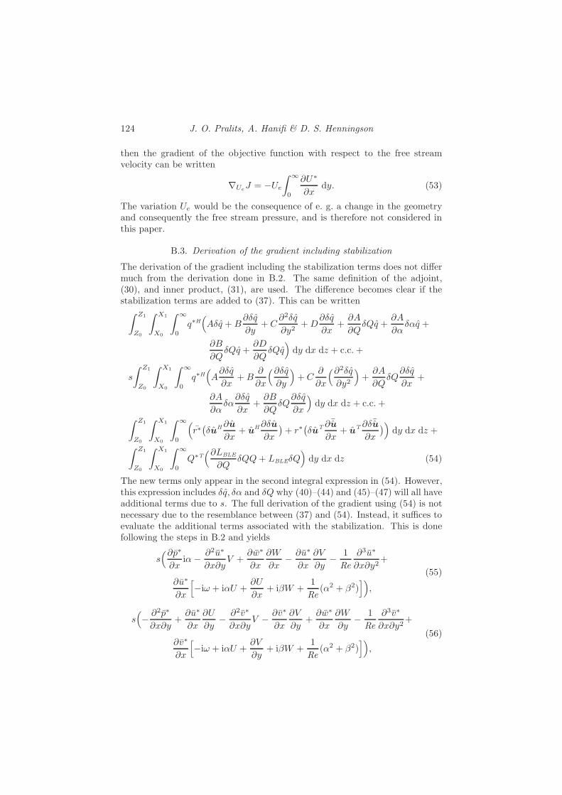
124 J. O. Pralits, A. Hanifi & D. S. Henningson
then the gradient of the objective function with respect to the free streamvelocity can be written
"UeJ = #Ue
* #
0
!U$
!xdy. (53)
The variation Ue would be the consequence of e. g. a change in the geometryand consequently the free stream pressure, and is therefore not considered inthis paper.
B.3. Derivation of the gradient including stabilization
The derivation of the gradient including the stabilization terms does not di!ermuch from the derivation done in B.2. The same definition of the adjoint,(30), and inner product, (31), are used. The di!erence becomes clear if thestabilization terms are added to (37). This can be written* Z1
Z0
* X1
X0
* #
0q$H&A0q + B
!0q
!y+ C
!20q
!y2+ D
!0q
!x+!A
!Q0Qq +
!A
!(0(q +
!B
!Q0Qq +
!D
!Q0Qq
'dy dx dz + c.c. +
s
* Z1
Z0
* X1
X0
* #
0q$H&A!0q
!x+ B
!
!x
&!0q!y
'+ C
!
!x
&!20q
!y2
'+!A
!Q0Q
!0q
!x+
!A
!(0(!0q
!x+!B
!Q0Q
!0q
!x
'dy dx dz + c.c. +
* Z1
Z0
* X1
X0
* #
0
&r$30uH !u
!x+ uH !0u
!x
4+ r$
30uT ! ¯u
!x+ uT !0¯u
!x
4'dy dx dz +
* Z1
Z0
* X1
X0
* #
0Q$T
&!LBLE
!Q0QQ + LBLE0Q
'dy dx dz (54)
The new terms only appear in the second integral expression in (54). However,this expression includes 0q, 0( and 0Q why (40)–(44) and (45)–(47) will all haveadditional terms due to s. The full derivation of the gradient using (54) is notnecessary due to the resemblance between (37) and (54). Instead, it su"ces toevaluate the additional terms associated with the stabilization. This is donefollowing the steps in B.2 and yields
s&!p$
!xi(# !2u$
!x!yV +
!w$
!x
!W
!x# !u$
!x
!V
!y# 1
Re!3u$
!x!y2+
!u$
!x
!#i* + i(U +
!U
!x+ i)W +
1Re
((2 + )2)"'
,
(55)
s&# !
2p$
!x!y+!u$
!x
!U
!y# !2v$
!x!yV # !v$
!x
!V
!y+!w$
!x
!W
!y# 1
Re!3v$
!x!y2+
!v$
!x
!#i* + i(U +
!V
!y+ i)W +
1Re
((2 + )2)"'
,
(56)
Optimization of steady suction for disturbance control 125
s&!p$
!xi) # !2w$
!x!yV # !w$
!x
!V
!y# 1
Re!3w$
!x!y2+
!w$
!x
!#i* + i(U + i)W +
1Re
((2 + )2)"'
,
(57)
s&!u$
!xi(# !2v$
!x!y+!w$
!xi)', (58)
s
* #
0
& !!x
!i(p$
!u
!x+ u$ !p
!x) + (iU +
2(Re
)(u$ !u
!x+ v$
!v
!x+ w$ !w
!x)"'
dy, (59)
s&real
(u$ !2u
!x!y# !v$
!y
!v
!x+ w$ !
2w
!x!y
)', (60)
s&real
(i([u$ !u
!x+ v$
!v
!x+ w$ !w
!x]# !
!x
&u$ !u
!x
'# !
!y
&u$ !v
!x
')', (61)
s&real
(i)[u$ !u
!x+ v$
!v
!x+ w$ !w
!x]# !
!x
&w$ !u
!x
'# !
!y
&w$ !v
!x
')'. (62)
Equations (55)–(58) are the additional terms in the (40)–(43) respectively.Equation (59) is the additional term in (44) and (60)–(62) are the additionalterms in (45)–(47) respectively. It should be noted here that the boundaryconditions do not change in any of the state or adjoint equations. Further, thegradient expression does not get any additional terms due to the stabilizationparameter s.
References
Airiau, C. 2000 Non-parallel acoustic receptivity of a Blasius boundary layer usingan adjoint approach. Flow, Turbulence Combust 65, 347–367.
Andersson, P., Berggren, M. & Henningson, D. 1999 Optimal disturbances andbypass transition in boundary layers. Phys. Fluids 11, 134–150.
Andersson, P., Henningson, D. S. & Hanifi, A. 1998 On a stabilization procedurefor the parabolic stability equations. J. Engng Maths 33, 311–332.
Balakumar, P. & Hall, P. 1999 Optimum suction distribution for transition pre-diction. Theor. Comput. Fluid Dyn. 13, 1–19.
Bertolotti, F., Herbert, T. & Spalart, S. 1992 Linear and nonlinear stabilityof the blasius boundary layer. J. Fluid Mech. 242, 441–474.
Bewley, T. & Liu, S. 1998 Optimal and robust control and estimation of linearpaths to transition. J. Fluid Mech. 365, 305–349.
Bewley, T. & Moin, P. 1997 Optimal and robust approaches for linear and non-linear regulation problems in fluid mechanics. AIAA Paper 97-1872.
Byrd, R., Lu, P., Nocedal, J. & Zhu, C. 1995 A limited memory algorithm forbound constrained optimization. SIAM J. Sci. Comput. 16, 1190–1208.

126 References
Dobrinsky, A. & Collis, S. S. 2000 Adjoint parabolized stability equations forreceptivity prediction. AIAA Paper 2000-2651.
Haj-Hariri, H. 1994 Characteristics analysis of the parabolized stability equations.Stud. Appl. Math. 92, 41–53.
Herbert, T. 1997 Parabolized stability equations. Annu. Rev. Fluid Mech. 29, 245–283.
Hill, D. C. 1997a Receptivity in non-parallel boundary layers. In ASME FluidsEngineering Division Summer Meeting, FEDSM ’97 .
Hill, D. C. 1997b Inverse design for laminar three-dimensional boundary layers.Bull. Am. Phys. Soc. 42, 2120.
Hogberg, M. & Berggren, M. 2000 Numerical approaches to optimal control ofa model equation for shear flow instabilities. Flow, Turbulence Combust 65,299–320.
Hogberg, M. & Henningson, D. S. 1998 Secondary instability of cross-flow vorticesin falkner-skan-cooke boundary layers. J. Fluid Mech. 368, 339–357.
Iglisch, R. 1949 Exakte berechnung der laminaren reibungsschicht an derlangsangestromten ebenen platte mit homogener absaugung. NACA RM 1205.
Joslin, R. 1998 Overview of laminar flow control. Tech. Rep. 1998-208705. NASA,Langley Research Center, Hampton, Virginia.
Li, F. & Malik, M. R. 1994 Mathematical nature of parabolized stability equa-tions. In 4th IUTAM Symp. on Laminar-Turbulent Transition, Sendi, Japan(ed. R. Kobayashi), pp. 205–212. Springer.
Li, F. & Malik, M. R. 1996 On the nature of pse approximation. Theor. Comput.Fluid Dyn. 8, 253–273.
Malik, M. R. & Balakumar, P. 1992 Nonparallel stability of rotating disk flowusing pse. In Instability, Transition and Turbulence (eds. M. Hussaini, A. Kumar& C. Streett), pp. 168–180. Springer.
Pralits, J. O., Airiau, C., Hanifi, A. & Henningson, D. S. 2000a Sensitiv-ity analysis using adjoint parabolized stability equations for compressible flows.Flow, Turbulence Combust 65, 321–346.
Pralits, J. O., Hanifi, A. & Henningson, D. S. 2000b Adjoint-based suctionoptimization for 3d boundary layer flows. Tech. Rep. FFA TN 2000-58. SwedishDefence Research Agency, FOI, Aeronautics Division, FFA, SE-172 90 Stock-holm, Sweden.
Schlichting, H. 1979 Boundary-Layer Theory , 7th edn. McGRAW-HILL.
Simen, M. 1992 Local and non-local stability theory of spatially varying flows. In In-stability, Transition and Turbulence (eds. M. Hussaini, A. Kumar & C. Streett),pp. 181–201. Springer.
Ulrich, A. 1944 Theoretishce untersuchungen uber die widerstandsersparnis durchlaminarhaltung mit absaugung. Schriften dt. Adad. d. Luftfahrtforschung 8B (2).
Walther, S., Airiau, C. & Bottaro, A. 2001 Optimal control of tollmien-schlichting waves in a developing boundary layer. Phys. Fluids 13, 2087–2096.
Zhu, C., Byrd, R., Lu, P. & Nocedal, J. 1994 L-bfgs-b: Fortran subroutines forlarge scale bound constrained optimization. Tech. Rep. NAM-11. EECS Depart-ment, Northwestern University.

Paper 3
3


Optimization of Steady Suction for DisturbanceControl on Infinite Swept Wings
By Jan O. Pralits1,2 and Ardeshir Hanifi2
We present a theory for computing the optimal steady suction distribution tosuppress convectively unstable disturbances in growing boundary layers on in-finite swept wings. This work includes optimization based on minimizing thedisturbance kinetic energy and the integral of the shape factor. Further, a suc-tion distribution in a continuous control domain is compared to an approachusing a number of discrete pressure chambers. In the latter case, the inter-nal static pressures of these chambers are optimized. Optimality systems arederived using Lagrange multipliers. The corresponding optimality conditionsare evaluated using the adjoint of the parabolized stability equations and theadjoint of the boundary layer equations. Results are presented for an airfoildesigned for medium range commercial aircraft. We show that an optimal suc-tion distribution based on a minimization of the integral of the shape factoris not always successful in the sense of delaying laminar-turbulent transition.It is also demonstrated that including di!erent types of disturbances, e. g.Tollmien-Schlichting and cross-flow types, in the analysis may be crucial.
1. IntroductionReducing the viscous drag on a wing while maintaining operational propertiessuch as lift for example, is of great interest and the research in this area isvast (see Joslin 1998). It is known that the viscous drag increases dramati-cally as the boundary layer flow changes from a laminar to a turbulent state.Therefore, a decrease in drag can be seen as increasing the laminar portionof the wing, or moving the point of laminar-turbulent transition downstream.Transition in the boundary layer on aircraft wings is usually caused by break-down of small disturbances which grow as they propagate downstream. Thegrowth of these disturbances can be analyzed using linear stability theory inwhich it is assumed that perturbations with infinitely small amplitude are su-perposed on the laminar mean flow. The growth rate can then be used topredict the transition location using the so called eN method (see van Ingen1956; Smith & Gamberoni 1956). Here it is assumed that transition will occurat the location where the total amplification of the disturbance, with respect
1Department of Mechanics, KTH, SE-100 44 Stockholm, Sweden.2Swedish Defence Research Agency, FOI, Aeronautics Division, FFA, SE-172 90 Stockholm,Sweden.
129

130 J. O. Pralits & A. Hanifi
to the first streamwise position where the disturbance starts to grow, attainsan empirically determined value, whose logarithm is generally denoted by N .
The stabilization e!ect of steady boundary layer suction on disturbancegrowth is well known (see Schlichting 1943/44) and has been utilized for lam-inar flow control, for an extensive review see Joslin (1998). However, in mostcases the design of suction distributions relies on the experience of the engi-neer which may not always give the optimal solution, i. e. to give the largestdelay of laminar-turbulence transition at a given suction power. In the last tenyears, the development of optimal control theory and its application to fluidmechanics problems has been rapid and a number of attempts have been madeto optimize the steady suction distribution in order to control the growth ofdisturbances, e. g. Hill (1997b); Balakumar & Hall (1999); Cathalifaud & Lu-chini (2000); Pralits et al. (2002); Airiau et al. (2003). In all of these works theoptimization methods are gradient based and utilize the potential of adjointmethods to obtain the gradients of interest. Other investigations includingthose by Mughal (1998); Walther et al. (2001); Hogberg & Henningson (2001)consider unsteady suction/blowing. This approach may not be suitable for flowcontrol on aircraft wings at the present time (see Bewley 2001) due to the com-plexity of its implementation. A common approach in the works by Balakumar& Hall (1999); Cathalifaud & Luchini (2000); Pralits et al. (2002); Airiau et al.(2003) is to minimize some measure of the disturbance growth, either the dis-turbance kinetic energy (see Cathalifaud & Luchini 2000; Pralits et al. 2002;Airiau et al. 2003) or the N -factor (see Balakumar & Hall 1999). The workby Airiau et al. (2003), in contrast to the others, did also try to minimize theshape factor which for 2D disturbances in a 2D boundary layer should resultin a suppression of disturbance amplification. Minimizing the shape factor isa more heuristic approach based on the knowledge that in such flows the two-dimensional disturbances are stabilized by any thinning of the boundary layer.Their results showed that an optimal suction distribution based on minimizingthe shape factor does have a damping e!ect on the disturbance growth. Theadvantage of this approach is that only one state equation has to be solvedwhich saves computational time. A negative aspect of not explicitly minimiz-ing a measure of the disturbances is that one cannot know if the computedsuction distribution will have a damping e!ect on the disturbances. This hasto be calculated afterwards, once the optimal suction distribution is obtained.
In Pralits et al. (2002) the idea of multi-disturbance control was intro-duced. The reason behind it is that, for certain types of flows, it is not clearwhich types of disturbances will be dominant in terms of amplification. Anexample is the Blasius flow in which, depending on the initial amplitudes, ei-ther two-dimensional Tollmien-Schlichting (TS) waves or streamwise streaksgrow the most. In three-dimensional boundary layers on wings there is usuallya streamwise region close to the leading edge with a strong negative pressuregradient, where cross-flow waves are the most amplified disturbances. Furtherdownstream, where the pressure gradient is zero or positive, TS waves are the

Optimization of Steady Suction 131
most amplified ones. When computing an optimal suction distribution it is alsonecessary to make sure that the mean flow modification due to a computed suc-tion distribution for a specific disturbance does not trigger the growth of otherdisturbances.
In real applications, steady boundary layer suction is usually done using anumber of discrete pressure chambers (see Reneaux & Blanchard 1992; Ellis &Poll 1996; Preist & Paluch 1996; Bieler & Preist 1992; Joslin 1998). In suchcases, the suction velocity is a function of the surface porosity, hole geometryand the pressure di!erence between the pressure distribution on the wing andstatic pressure in the chambers (see Bieler & Preist 1992; Preist & Paluch1996). This means that the size, position and the internal static pressure ofeach chamber are the design variables. The suction distribution is then givenby the specific choice of these parameters. Atkin (2000) used an engineeringapproach to design of the suction system in which he utilized the stabilitycharacteristics of the flow. Here, the static pressure in the pressure chambers,based on an automatized trial and error technique, were chosen such that theamplification of disturbances stayed under a specified value.
Most of the previous works such as Balakumar & Hall (1999); Cathal-ifaud & Luchini (2000); Pralits et al. (2002); Airiau et al. (2003) on optimalsteady suction deal with incompressible boundary layer flows on flat plates. Hill(1997b) analyzed an infinite swept wing for inverse design of laminar boundarylayers but no details were given of how this was done. The considered suctiondistributions have been applied in a continuous (see Balakumar & Hall 1999;Cathalifaud & Luchini 2000; Pralits et al. 2002; Airiau et al. 2003) or a num-ber of discrete control domains (see Airiau et al. 2003). However, so far nostudy has shown how to incorporate the use of pressure chambers in order toapproach a real application.
In this paper we extend the work by Pralits et al. (2002), to compressibleboundary flows on infinite swept wings. Here we compare the case of mini-mizing the disturbance kinetic energy with the simplified approach by Airiauet al. (2003) of minimizing the integral of the shape factor. The feasibilityof the control is addressed by comparing two di!erent ways of computing thesuction distribution: a continuous distribution of mass flux on the wall in acontrol domain, and a number of discrete pressure chambers, which constitutesa more realistic approach to obtaining a suction distribution on the wall. Theevolution of disturbances is analyzed using the Parabolized Stability Equations(PSE) (see Bertolotti et al. 1992; Malik & Balakumar 1992; Simen 1992; Her-bert 1997), and the laminar mean flow is computed using the two-dimensionalthree-component boundary layer equations (BLE). We use optimal control the-ory, in which the aim is to minimize a given objective function with state equa-tions and the control energy as constraints. The problem is solved using aLagrange multiplier technique, which yields an optimality system consisting ofstate and corresponding adjoint equations from which an optimality conditionis evaluated. Here, we couple the adjoint of the PSE with the adjoint of the

132 J. O. Pralits & A. Hanifi
Q V
U
x
x
x
1
2
3
Figure 1. Definition of the coordinates for the infinite swept wing.
boundary-layer equations in order to find the optimality condition. The deriva-tion of the optimality system is similar to that presented in Pralits et al. (2002)and is therefore presented here in a more compact form. Results are presentedfor control of disturbance growth in a boundary layer on a wing designed forcommercial aircraft.
2. Problem formulationThe flow field considered here is the boundary layer on a swept wing with in-finite span which is obtained by solving the mass, momentum and energy con-servation equations for a viscous compressible fluid. The equations are writtenin an orthogonal curvilinear coordinate system with streamwise, spanwise andwall-normal coordinates denoted as x1, x2 and x3 respectively, see Fig. 1. Alength element is defined as ds2 = (h1dx1)2 + (h2dx2)2 + (h3dx3)2 where hi isthe scale factor. The total flow field, qtot is decomposed into a mean, q, and aperturbation part, q, as
qtot(x1, x2, x3, t) = q(x1, x3) + q(x1, x2, x3, t)
where q ' [U, V, W, P, T, "] and q ' [u, v, w, p, T , "]. Here U, V, W are thestreamwise, spanwise and wall-normal velocity components of the mean flowrespectively, T is the temperature, " the density and P the pressure. Therespective lower case variables correspond to the disturbance quantities. Theequations are derived for a quasi three-dimensional mean flow with zero vari-ation in the spanwise direction. The evolution of convectively unstable dist-urbances is analyzed in the framework of the nonlocal stability theory. Themean flow and disturbance equations in the following sections are given indimensionless form. All flow and material quantities are made dimensionlesswith the corresponding reference flow quantities at a fixed streamwise positionx!
0, except the pressure, which is referred to twice the corresponding dynamicpressure. Here, dimensional quantities are denoted by the superscript 4.
The reference length scale is taken as l!0 = (&!0x!
0/U!0 ) 1
2 . The Reynolds andMach number are defined as Re = l!0U
!0 /&!
0 and M = U!0 /(R%T !
0 ) 12 respectively
where R is the specific gas constant, & the kinematic viscosity and % the ratio

Optimization of Steady Suction 133
of the specific heats. In the proceeding sections the scale factors h2, h3 = 1 aredue to the infinite swept wing assumption.
2.1. Mean-Flow equations
The dimensionless boundary layer equations (BLE) written in primitive vari-able form can be seen in Appendix A and are here written in symbolic formas
LB Q = 0 (1)
where Q = (U, V, W, T )T. The suction distribution is imposed using the wallnormal velocity component at the wall Ww(x1) = W (x1, x3). Non slip condi-tions are applied to the other velocity components and we assume an adiabaticwall condition for the temperature. Equation (1) is integrated from the stagna-tion point in the downstream direction normal to the leading edge. Note thatfor the boundary layer approximation to be valid, the wall normal velocity atthe wall, Ww, should be of O(Re"1). Here, it is assumed that the pressure dis-tribution on the airfoil does not change as the suction distribution is applied.If the suction distribution would result in a large change in the boundary layerthickness, then it might be necessary to update the pressure distribution in theoptimization process.
2.2. Disturbance equations
The perturbations are assumed to be time and spanwise periodic waves as
q(xi, t) = q(x1, x3)$, where $ = exp
+i* x1
X0
((x!)dx! + i)x2 # i*t
,. (2)
Here ( is the complex streamwise wavenumber, ) the real spanwise wavenumberand * the real disturbance angular frequency. X0 is the initial streamwiseposition where the disturbances are superimposed on the mean flow. We assumea scale separation Re"1 between the weak variation in the x1-direction and thestrong variation in the x3-direction. Further, it is assumed that !/!x1 4O(Re"1) and W 4 O(Re"1). Introducing the ansatz given by Eq. (2) andthe assumptions above in the linearized governing equations, yields a set ofnearly parabolic partial di!erential equations (see Bertolotti et al. 1992; Malik& Balakumar 1992; Simen 1992; Herbert 1997). The system of equations,denoted parabolized stability equations (PSE), can be seen in Appendix A andare here written in symbolic form as
LP q = 0, (3)
where q = (", u, v, w, T )T. Here u, v, w and T are subject to Dirichlet bound-ary conditions. To remove the ambiguity of having x1-dependence of both theamplitude and wave function in the ansatz, and to maintain a slow stream-wise variation of the amplitude function q, a so called ’auxiliary condition’ is

134 J. O. Pralits & A. Hanifi
introduced * +#
0qH !q!x1
dx3 = 0, (4)
where superscript H denotes the complex conjugate transpose. Equation (3)is integrated in the downstream direction normal to the leading edge withan initial condition given by local stability theory. At each x1-position thestreamwise wavenumber ( is iterated such that the condition given by Eq.(4) is satisfied. After a converged streamwise wavenumber has been obtained,the growth rate of the disturbance kinetic energy can be calculated from thefollowing relation
+ = #(i +!
!x1(ln)
E),
where
E =* +#
0" (|u|2 + |v|2 + |w|2) dx3.
The growth rate can then be used to predict the transition location using theso called eN -method (see van Ingen 1956; Smith & Gamberoni 1956). TheN -factor based on the disturbance kinetic energy is given as
NE =* X
Xn1
+ dx1,
where Xn1 is the lower branch of the neutral curve. A complete description ofEq. (3) is found in Pralits et al. (2000), and corresponding numerical schemesused here are given in Hanifi et al. (1994).
3. Optimal controlThe approach of the current work is to use optimal control theory to findthe optimal mean flow suction distribution in order to suppress the growthof convectively unstable disturbances. In this paper we investigate di!erentcontrol variables and objective functions. First, a general introduction is givenin this section. Then follows a concise description of the Lagrange multipliertechnique applied to the problem of minimizing a measure of the disturbancesusing the mass flux on the wall (mw = Ww"w) as control variable.
The problem consists of the state variables Q and q; a control variablegiven by the mass flux on the wall; constraints on the state variables given bythe BLE and PSE; and an objective function, a measure of the state, to beminimized.
The final goal of boundary-layer suction is to increase the laminar portionof the wing i. e. to move the location of laminar-turbulent transition furtherdownstream, and thus decrease the viscous drag. It is therefore important thatthe chosen objective function can be related to the transition process. Onechoice is to measure the kinetic energy of a certain disturbance at a downstream

Optimization of Steady Suction 135
position, say Xf . This can be written as
Ef =12
* Z1
Z0
* +#
0qHM q h1dx2dx3
11111x1=Xf
, (5)
where M = diag(0, 1, 1, 1, 0) which means that the disturbance kinetic energyis calculated from the disturbance velocity components. Hanifi et al. (1996)used a measure which also included " and T . If the position Xf is chosen asthe upper branch of the neutral curve, then the measure can be related to themaximum value of the N -factor (see Airiau et al. 2003). If in addition, thevalue of the N -factor of the measured disturbance is the one which first (withzero control) reaches the transition N -factor, then the position can be relatedto the onset of laminar-turbulent transition. It is however not clear, a priori,that such a measure will damp the chosen disturbance or other ones in thewhole unstable region, especially if di!erent types of disturbances are present,such as TS and cross-flow waves. For Blasius flow, it has been shown that anobjective function based on a single TS wave is su"cient to successfully dampthe growth of other TS waves (see Pralits et al. 2002; Airiau et al. 2003). On awing however, it is common that both TS and cross-flow waves are present. Analternative is therefore to measure the kinetic energy as the streamwise integralover a defined domain. Using such an approach several di!erent disturbances,with respective maximum growth rate at di!erent positions, can be accountedfor in the same domain. Here, the size of K disturbances superimposed onthe mean flow at an upstream position X0, is measured by their total kineticenergy as
E! =K%
k=1
12
* Xme
Xms
* Z1
Z0
* +#
0qH
kM qkh1dx1dx2dx3. (6)
We now define the objective function based on the disturbance growth as
J0 = ,E! + (1# ,)Ef , (7)
where the parameter , can be chosen between zero and one, depending on thequantity one wants to minimize. In order to have a well-posed problem, thecontrol needs to be bounded. This is done by quantifying the control e!ort as
EC =* Xce
Xcs
m2wh1dx1. (8)
This measure has a physical meaning and also enables comparison of e"ciencyof di!erent objective functions. Taking the square of mw means that bothblowing and suction will be accounted for in EC .
A concise description of the objective can now be made: find the controlmw, and corresponding states Q and q which minimizes the objective functionJ0 with the constraints given by Eqs. (1), (3), (4) and (8). We now usea Lagrange multiplier technique to replace the original constrained problemwith an unconstrained one, see e. g. Gunzburger (1997). In order to enforce

136 J. O. Pralits & A. Hanifi
the constraints we introduce the adjoint variables Q$,q$, r$,#$,3$ and theLagrangian functional
L = J0 # J1 (9)
where
J1 = -Q$, LB Q.+* Xce
Xcs
#$8m(x1, 0)# mw
9h1dx1
+ 3$(EC #* Xce
Xcs
m2wh1dx1) + -q$, LP q.+ -r$q,
1h1
!q!x1.+ c.c.
where c.c. denotes the complex conjugate. The inner products -·, ·. appearingabove are defined as
-/,5. =* X1
X0
* Z1
Z0
* +#
0/H5 h1dx1dx2dx3, (10)
for complex valued vectors / and 5. We can now define the problem as: findthe control mw, states Q, q and adjoint variables #$,3$,Q$,q$ and r$ suchthat L is rendered stationary according to the first-order necessary conditionfor an extremal point. This is done by setting the first variation of L withrespect to the variables considered here to zero, while each of L’s argumentsare considered to be independent variables. This requirement comes from thefact that at an extremal point the first variation of L with respect to eachvariable vanishes. We start by setting the first variation of L with respect toeach adjoint variable to zero, which gives the state equations (1), (3) and (4),and the constraint on the control e!ort, Eq. (8). We continue by setting thefirst variation of the state variables q, ( and Q to zero. After a procedurewhich involves successive integrations by parts (see Pralits et al. 2002), thisyields the adjoint equations
L$P q$ = S$
P, (11)
!
!x1
* +#
0q$H !LP
!(qh1dx3 =
@A
B
0 0x1 /' [Xms, Xme]
#i|$|2* +#
0qHM qh1dx3 0x1 ' [Xms, Xme],
(12)L$
B Q$ = S$B, (13)
where q$ = ("$, u$, v$, w$, '$)T and Q$ = (U$, V $, W $,T $)T. Equation (11) isthe adjoint of the PSE (APSE) where u$, v$, w$ and '$ are subject to Dirichletboundary conditions. The right hand side S$
P is due to the auxiliary conditionof the PSE and the objective function. Equation (12) is a closure relationobtained by setting the first variation of L with respect to the streamwisewavenumber ( to zero. At each streamwise position, r$ is solved iterativelysuch that Eq. (12) is satisfied. Equation (13) is the adjoint of the BLE (ABLE)and the right hand side S$
B is the sensitivity of the PSE with respect to themean flow. Both the APSE and ABLE are parabolic equations which are solved
Optimization of Steady Suction 137
by backward integration in the streamwise direction. The above equations arefound in A.1, and the complete derivations are found in Pralits et al. (2000)and Pralits (2001). Finally, we set the first variation of L with respect to mw
to zero which gives the so called optimality condition as
W $w + 23$mw = 0. (14)
The left hand side of the above expression is the gradient of the Lagrangianfunctional with respect to the mass flux at the wall. As shown in Eq. (9),3$ is the adjoint variable used to enforce the control e!ort and can be solvediteratively in the optimization by substituting Eq. (14) into Eq. (8) as
3$ =
+1
4EC
* Xce
Xcs
W $2w h1dx1
, 12
. (15)
The complete optimality system contains Eqs. (1), (3), (4) and (11)–(15) whichcan be found in Appendix A.
3.1. Solution procedure
The procedure of solving the optimization problem derived in Sec. 3 is de-scribed here. We start by considering the case of minimizing a single distur-bance, i. e. K = 1 in Eq. (6).
The optimal distribution of the mass flow is found through an iterativeprocedure. During each iteration step, we perform successive calculations ofboundary-layer and stability equations from X0 to X1; and adjoint boundary-layer and stability equations from X1 to X0. Then, a new mass-flow distributionis computed using the gradient information given by solution of the adjointequations. Here we use the L-BFGS-B optimization routine, see Zhu et al.(1994) and Byrd et al. (1995). The calculations are repeated until the relativechange in the objective function is less than a prescribed value.
If K > 1 in Eq. (6) then instead of solving both state and adjoint equationsK times, we can utilize the fact that the ABLE are linear equations. In this casethe optimality condition is evaluated as follows: the BLE is solved once; thePSE and APSE are solved K times; the forcing of the ABLE, S$
B, is calculatedas
S$B =
K%
k=1
S$Bk
.
Finally, the optimality condition is evaluated from a single calculation of theABLE.
The results presented here are obtained by numerically integrating thediscretized state and adjoint equations. The x1-derivatives are approximatedby a first- or second-order accurate backward Euler scheme. The x3-derivativesof the PSE and APSE are approximated by a fourth-order accurate compactfinite-di!erence scheme and a second-order accurate finite-di!erence schemefor the BLE and ABLE. The convergence criteria is (J k+1 # J k)/J k < 10"4,

138 J. O. Pralits & A. Hanifi
0 0.2 0.4 0.6 0.8 1−1
−0.5
0
0.5
1
1.5
−Cp
s/c
Figure 2. The pressure distribution, Cp, as a function of thearc-length normal to the leading edge, s/c. The black boxshows the available control domain, (c.
where k denotes the iteration number in the optimization procedure. Further,in all calculations the initial guess on the suction profile, min
w , has been variedto make sure that the optimal solution does not depend on the initial state.
3.2. Case studied
The flow studied here is the boundary layer on the upper side of a wing designedfor commercial aircraft. The flow conditions are characterized by a free streamMach number M# = 0.8, temperature T# = 230 K, Reynolds number Re# =3.04 ( 107 and leading edge sweep angle 5le = 30.2(. The control domain,(c = [Xcs, Xce], available for mounting the suction-system has been specifiedby the manufacturer. The control domain is limited in the upstream direction,0 < s/c < 0.006, by a suction strip used to control the stagnation line andin the downstream direction by the front spar (s/c=0.17). Here s is the arc-length normal to the leading edge measured from the stagnation point and cis the chord length. The suction strip at the stagnation line is case specificand will be held unchanged. However, this does not create any di"culties inthe optimization procedure. In Fig. 2 the pressure coe"cient Cp is plottedas a function of s/c. The available control domain 0.006 + s/c + 0.17 is alsoindicated in this figure as a black box.
Parameters for the disturbances analyzed here are given in Table 1. At theinitial streamwise position (s/c = 0.0075), the flow has a strong favorable pres-sure gradient and the mean flow velocity component perpendicular to the outerstreamline has an inflection point. There, waves with the wavenumber vector kapproximately perpendicular to the outer streamline have positive growth rate.These are the so called cross-flow (CF) waves. Further downstream (s/c = 0.05)where the pressure gradient is weaker and adverse, Tollmien-Schlichting (TS)

Optimization of Steady Suction 139
X0 f$ %f$ )$ %)$ Type0.0075 [1000, 8500] 500 [1000, 6000] 500 CF0.0075 0 0 [500, 6500] 500 CF0.05 [2250, 9500] 250 0 0 TS0.05 [2250, 7000] 250 [25, 225] 50 TS
Table 1. Initial position (s/c = X0), dimensional frequency(f$), dimensional spanwise wave number ()$) and type of dist-urbances analyzed (CF = cross-flow wave, TS = Tollmien-Schlichting wave). %f$ and %)$ denote respective dimensio-nal step-length.
0 0.1 0.2 0.3 0.4 0.50
4
8
12
16
NE
s/c
CF
TS
Figure 3. Envelope of envelopes of NE-factor curves for thetwo disturbance types given in table 1 for the case of zerosuction.
waves are amplified. The angles between the wavenumber vectors of the TSwaves analyzed here and the outer streamline are 0 # 60 degrees. In Fig. 3,the envelope of envelopes (EoE) of the NE-factor curves are plotted for the CFand TS disturbances given in Table 1 and for zero suction rate.
The control e!ort which is quantified by Eq. (8) depends on the specificsuction system chosen, i. e. compressors and tubing. We have therefore chosena number of di!erent magnitudes of EC to examine the dependency of theachieved stabilization on the amplitude of the control energy. Here we introducea new parameter QC = ECRe#. In our calculations the values of QC are chosenso that a noticeable control e!ect is achieved and to avoid the magnitude ofmean wall-normal velocity (at the wall) Ww exceeding O(Re"1). This waschecked after each calculation.

140 J. O. Pralits & A. Hanifi
0 0.05 0.1 0.15 0.2−20
−15
−10
−5
0
5
mw
# 1
04
s/c
.
Figure 4. Optimal suction distributions, mw, minimizing thedisturbance kinetic energy of a CF wave (f$ = 5500 s"1, )$ =2500 m"1) measured as E! (dashed), Ef (solid). QC = 0.35and 0.58, and the arrow marks increasing QC .
3.3. Results
Results are shown here for minimization of the disturbance kinetic energy, Eq.(5.17), in which , has been chosen depending on the desired objective function.In the latter, the measure is given as the sum of the kinetic energy of K dist-urbances. Before the optimization is performed, it has to be decided if one orseveral disturbances should be included. One of the conclusions from Pralitset al. (2002) and Airiau et al. (2003) was that the optimal suction distributionfor a given disturbance will also have a damping e!ect on other disturbancesof the same type. The reason for including more than one disturbance in themeasure (see Pralits et al. 2002) is that in some cases it is not clear which typeof disturbance will cause laminar-turbulent transition first. Another reason isthat if di!erent types of disturbances are present in the flow, then the meanflow modification that minimizes some measure of one type of disturbance mayamplify rather than damp disturbances of another type. One should keep inmind that the larger number of disturbances considered, the more costly theoptimization procedure will be. As a first investigation, a comparison is madebetween minimizing the kinetic energy of a single disturbance integrated in astreamwise domain (, = 1), with the case of minimizing the same disturbanceat a final streamwise position (, = 0). Eq. (5.16) is integrated between X0 andthe end of the control domain which means that the aim is to delay transitionat least up to this position. Xf in Eq. (5.14) is chosen as the position wherethe maximum disturbance kinetic energy is found over all disturbances in Ta-ble 1, here Xf = 0.105. The corresponding disturbance, which also has thelargest E! over all disturbances in Table 1, is chosen as the one to minimizein both cases. This disturbance is a CF wave with dimensional frequency and

Optimization of Steady Suction 141
0 0.1 0.2 0.3 0.4 0.52
2.5
3
3.5
4
4.5
s/c
H12
Figure 5. Shape factor, H12, given zero (dotted) and optimalsuction distribution from Fig. 4 minimizing the disturbancekinetic energy of a CF wave (f$ = 5500 s"1, )$ = 2500 m"1)measured as E! (dashed), Ef (solid). QC = 0, 0.35 and 0.58,and the arrow marks increasing QC .
spanwise wave number of 5500 s"1 and 2500 m"1, respectively. The calcula-tions are performed for QC = 0.25, 0.35, 0.45 and 0.58. The optimal suctiondistributions given by the two di!erent objective functions can be seen in Fig.4. Here, results are only shown for two di!erent values of the control energyto make the plot more clear. The arrow indicates the direction of increasingQC and the uppermost streamwise suction distribution is the fixed stagnationline control. It is interesting to note the similarity between the results whencomparing the two objective functions as opposed to a similar comparison forcontrol of TS waves reported by Airiau et al. (2003). The reason for this maybe that the growth and decay of CF waves in the case analyzed here occursover a short streamwise interval, and as a consequence the growth measuredby E! approach that for Ef . In all cases, the optimal control acts primarilyin the region where a strong favorable pressure gradient exists and then decaysfurther downstream. As the control e!ort is increased, the additional controlenergy is concentrated to the beginning of the control domain. The e!ect ofthe control on the shape factor is however small, which can be seen in Fig.5. The magnitudes of the suction distributions presented in this paper areall within the range of validity for the boundary layer equations, i. e. of orderO(Re"1). This was investigated by Airiau et al. (2003), where suction distribu-tions with magnitudes within the limits experienced locally rapid streamwisevariations. They compared solutions from the Navier-Stokes equations withthose using the boundary layer equations. They found that the pressure gra-dient from the Navier-Stokes solution varies rapidly close to the suction peakbut relaxes very rapidly downstream where it becomes small, in accordance

142 J. O. Pralits & A. Hanifi
0 0.1 0.2 0.3 0.4 0.50
4
8
12
16
20
NE
s/c
CF
TS
Figure 6. Envelope of envelopes of NE-factor curves for thedisturbances given in table 1 given zero (dotted) and optimalsuction distribution from Fig. 4 minimizing the disturbancekinetic energy of a CF wave (f$ = 5500 s"1, )$ = 2500 m"1)measured as E! (dashed), Ef (solid). QC = 0, 0.35 and 0.58,and the arrows mark increasing QC .
with the parabolic assumption of the boundary layer equations. They furthershowed that shape factors from the boundary layer and Navier-Stokes solutionsagree well and conclude that there is a weak dependence of the shape factoron the mean pressure gradient and that the solutions of the boundary-layerequations are valid. In Fig. 6, the EoE of the NE-factor curves of CF andTS waves are plotted for the cases of zero and optimal suction distributionsshown in Fig. 4. In the control domain, the CF waves are more damped asQC is increased. However, downstream of the control region the CF waves areincreasingly amplified as QC is increased. As expected the TS waves are lessa!ected by the controls since we know that the control acts upstream of theregion where the TS waves are amplified. In the results shown here, the op-timal suction distributions are based on minimizing a single disturbance only.The damping e!ect of such a control on other disturbances of the same typecan be seen from EoE curves given in Fig. 6. In Figs. 7 and 8, this has beenemphasized by plotting contours of E! for CF and TS waves in the (f$,)$)-plane comparing zero and optimal suction distributions for all values of QC .In all cases the kinetic energy of all disturbances has been reduced. It is clearfrom the ratio between the maximum value of E! for the zero and optimalcontrol, that the CF waves are mostly a!ected. This is true for all values ofQC studied here. From these results, as discussed in Pralits et al. (2002) andAiriau et al. (2003), one can conclude that minimizing the disturbance kineticenergy of one disturbance (in this case CF waves) does have a damping e!ecton other disturbances of the same type. To confirm this, computations were

Optimization of Steady Suction 143
0 2000 4000 6000 80000
2000
4000
6000
8000
%*
f*
(a)
0 2000 4000 6000 80000
2000
4000
6000
8000
%*
f*
(b)
0 2000 4000 6000 80000
2000
4000
6000
8000
%*
f*
(c)
0 2000 4000 6000 80000
2000
4000
6000
8000
%*
f*
(d)
Figure 7. Contours of E! for CF waves comparing zero(solid) and optimal suction distribution (dashed) minimizingthe disturbance kinetic energy of a CF wave (f$ = 5500 s"1,)$ = 2500 m"1). Both cases are normalized with their re-spective maximum value and the contour spacing = 0.1. Thecontrol e!ort QC and the ratio between the maximum valuesare respectively (a) 0.25, 1.4( 10"8; (b) 0.35, 6.7( 10"10; (c)0.45, 6.4( 10"11; (d) 0.58, 5.5( 10"12.
also performed in which the TS wave with the largest total disturbance kineticenergy was controlled. The suction distribution from these calculations hada damping e!ect on all other TS waves. These results are not shown here.The absence of control in the region where the TS waves are amplified can beovercome by adding a disturbance of TS type in the objective function when, = 1. Therefore, as a next step both the CF and TS wave with the largestE! over all respective disturbances in Table 1 are considered. The dimensionalfrequency and spanwise wave number for the TS wave are 5750 s"1 and 225m"1, respectively, and the calculations are performed with the same values of

144 J. O. Pralits & A. Hanifi
0 50 100 150 2004000
5000
6000
7000
%*
f*
(a)
0 50 100 150 2004000
5000
6000
7000
%*
f*
(c)
0 50 100 150 2004000
5000
6000
7000
%*
f*
(b)
0 50 100 150 2004000
5000
6000
7000
%*
f*
(d)
Figure 8. Contours of E! for TS waves comparing zero(solid) and optimal suction distribution (dashed) minimizingthe disturbance kinetic energy of a CF wave (f$ = 5500 s"1,)$ = 2500 m"1). Both cases are normalized with their re-spective maximum value and the contour spacing = 0.1. Thecontrol e!ort QC and the ratio between the maximum valuesare respectively (a) 0.25, 0.21; (b) 0.35, 0.16; (c) 0.45, 0.1; (d)0.58, 0.092.
QC used for control of a single CF wave. In Table 2 the ratio between themaximum values of E! for CF waves using optimal and zero suction are given.Here, we compare the case of optimal suction based on minimizing a CF wavewith the case of minimizing the sum of a CF and a TS wave. It is seen thatthe change of the ratio is small between the cases, even when QC is increased.In Table 3 the same comparison is done for the ratio of the maximum values ofE! for TS waves. Here, it is clear that the ratio has decreased when both CFand TS disturbances are considered. As the same amount of control e!ort isused, this means that QC is redistributed in the streamwise direction to control

Optimization of Steady Suction 145
Disturbance QC = 0.25 QC = 0.35 QC = 0.45 QC = 0.58CF 1.4( 10"8 6.7( 10"10 6.4( 10"11 5.5( 10"12
CF+TS 2.2( 10"8 1.4( 10"9 5.7( 10"11 1.1( 10"11
Table 2. Ratio between maximum values of E! for CF waveswhen zero and optimal suction distribution minimizing thedisturbance kinetic energy is applied. The ratio is calculatedwhen equation (5.16) includes CF and CF+TS for di!erentvalues of QC .
Disturbance QC = 0.25 QC = 0.35 QC = 0.45 QC = 0.58CF 2.1( 10"1 1.6( 10"1 1.0( 10"1 9.2( 10"2
CF+TS 6.1( 10"3 8.6( 10"3 1.1( 10"3 6.6( 10"5
Table 3. Ratio between maximum values of E! for TS waveswhen zero and suction distribution control minimizing the dis-turbance kinetic energy is applied. The ratio is calculatedwhen equation (5.16) includes CF and CF+TS for di!erentvalues of QC .
the TS wave. The corresponding optimal suction distributions are plotted inFig. 9 for the cases when EC=0.35 and 0.58. The suction distributions in theupstream part of the control domain are similar to the ones in Fig. 4, but themagnitudes are smaller. Further downstream, the suction distribution is ratherconstant before it goes to zero at the end of the control domain. The latter issimilar to what is shown in Pralits et al. (2002) for control of two-dimensionalTS waves in two-dimensional boundary layer flows when a small control e!ortis used. The e!ect of the control on the shape factor is plotted in Fig. 10.Compared to the results given in Fig. 5, a larger decrease of H12 occurs in thedownstream portion of the control domain. The corresponding thinning of theboundary layer is favorable in terms of damping the TS waves. The EoE of theNE-factor curves are plotted in Fig. 11. Here, the CF waves are less dampedcompared to the previous case, see Fig. 6. However, the TS waves are nowmore damped.
It is of interest to know if a larger reduction of the disturbance kineticenergy can be obtained for a given control e!ort if additional modes, apartfrom the two discussed here, are included in the calculations. Such a parameterstudy has been performed and the results show that the additional decrease indisturbance kinetic energy is small when more modes are included. The reasonis that the control mainly acts on the modes with the largest energy. Since thecontrol a!ects all other disturbances (shown here), it will continue to act on themode with the initially largest energy even if additional modes are included.

146 J. O. Pralits & A. Hanifi
0 0.05 0.1 0.15 0.2−20
−15
−10
−5
0
5
mw
# 1
04
s/c
.
Figure 9. Optimal suction distributions, mw, minimizing thedisturbance kinetic energy E! of a CF (f$
1 = 5500 s"1, )$1 =
2500 m"1) and TS wave (f$2 = 5750 s"1, )$
2 = 225 m"1). QC= 0.35 and 0.58, and the arrow marks increasing QC .
0 0.1 0.2 0.3 0.4 0.52
2.5
3
3.5
4
4.5
s/c
H12
Figure 10. Shape factor, H12, given zero (dotted) and opti-mal suction distribution (solid) from Fig. 9 minimizing the dis-turbance kinetic energy E! of a CF (f$
1 = 5500 s"1, )$1 = 2500
m"1) and TS wave (f$2 = 5750 s"1, )$
2 = 225 m"1). QC = 0,0.35 and 0.58, and the arrow marks increasing QC .
4. Simplified approachIn design of suction distributions for the purpose of delaying laminar-turbulenttransition, it is important that the procedure is not computationally expensive.The same argument can be made when designing on-line control systems, where

Optimization of Steady Suction 147
0 0.1 0.2 0.3 0.4 0.50
4
8
12
16
NE
s/c
CF
TS
Figure 11. Envelope of envelopes of NE-factor curves for thedisturbances given in table 1 given zero (dotted) and optimalsuction distribution from Fig. 9 minimizing the disturbancekinetic energy E! of a CF (f$
1 = 5500 s"1, )$1 = 2500 m"1)
and TS wave (f$2 = 5750 s"1, )$
2 = 225 m"1). QC = 0, 0.35and, 0.58 and the arrows mark increasing QC .
fast feed back is needed. For this purpose, an alternative approach was analyzedin Airiau et al. (2003) for the control of TS waves in incompressible flat-plateboundary layers. In their study the optimal suction distribution is computedby minimizing the streamwise integral of the shape factor. This means thatonly the boundary layer and corresponding adjoint equations are involved inthe optimization process which is computationally more e"cient. However, thee!ect of the optimal suction distribution on the disturbance growth is analyzedafterwards. This choice of objective function is based on the knowledge that anythinning of the boundary layer has a stabilizing e!ect on the boundary layer.Successful results are shown for control of TS waves. The positive features ofthis approach motivates an investigation here.
4.1. Optimality system
The objective function is now given as
J0 =* Xme
Xms
H12h1dx1, whereH12 =0102
=
* +#
0
-1# "USL
"eQe
.dx3
* +#
0
"USL
"eQe
-1# USL
Qe
.dx3
. (16)
Both the displacement 01 and momentum thickness 02 are based on the velocitycomponent USL = U cos(5) + V sin(5) which is in the direction of the outerstreamline. Here 5 = tan"1(Ve/Ue) and Qe = (Ue
2 + Ve2) 1
2 . Now, only onestate equation is considered and the problem consists of finding the control mw,

148 J. O. Pralits & A. Hanifi
0 0.1 0.2 0.3 0.4 0.52
2.5
3
3.5
4
4.5
s/c
H12
Figure 12. Shape factor, H12 for zero (dotted) and optimalsuction distributions (solid) minimizing the shape factor. QC= 0, 0.1, 0.3, 0.58, 0.81 and 1.43 and the arrows mark increas-ing QC .
and corresponding state Q which minimizes J0 given the constraints shown inEqs. (1) and (8). The technique using Lagrange multipliers is also used hereto enforce the constraints. The adjoint variables Q$,#$,3$ are introduced andthe new Lagrangian functional is given as
L = J0 # J1 (17)
where J1 is now written
J1 = -Q$, LB Q.+* Xce
Xcs
#$8m(x1, 0)# mw
9h1dx1 +
3$(EC #* Xce
Xcs
m2wh1dx1).
The derivation is performed as previously described which yields an optimalitysystem which contains the BLE, Eq. (1), corresponding adjoint equation andoptimality condition. Compared to the previously derived ABLE, di!erencesoccur in the boundary conditions and forcing term S$
B. These di!erences aredue to the objective function, Eq. (16). Details of the optimality system canbe seen in Appendix B.
4.2. Results
Results are shown here on minimizing the shape factor. First we consider con-trol in the whole available domain (c, and the objective function is integratedin the same streamwise region used for Eq. (5.16) in Sec. 3.3. The controle!orts in these calculations are QC = 0.1, 0.3, 0.58, 0.81 and 1.43. In Fig.12 the shape factors for these cases are compared to that of the uncontrolled

Optimization of Steady Suction 149
0 0.05 0.1 0.15 0.2−20
−15
−10
−5
0
5
mw
# 1
04
s/c
.
Figure 13. Optimal suction distributions, mw, minimizingthe shape factor, H12. QC = 0.1, 0.3, 0.58, 0.81, 1.43 and thearrows mark increasing QC .
0 0.1 0.2 0.3 0.4 0.50
4
8
12
16
20
NE
s/c
CF
TS
Figure 14. Envelope of envelopes of NE-factor curves for thetwo disturbance types given in table 1 given zero (dotted) andoptimal suction distribution minimizing (solid) the shape fac-tor. QC = 0, 0.1, 0.3, 0.58, 0.81, 1.43 and the arrows markincreasing QC .
case. As the control e!ort is increased, the shape factor is decreased within themajor part of the control domain. Downstream of the control domain a smallincrease of the shape factor is observed.
The corresponding suction profiles are plotted in Fig. 13. Note that theuppermost streamwise suction distribution is due to the stagnation line controlwhich is taken to be fixed. In all cases, the optimal control is divided roughly at

150 J. O. Pralits & A. Hanifi
0.05 0.1 0.15−3
−2
−1
0
1
mw
# 1
04
s/c
.
Figure 15. Comparison of optimal suction distributions forthe cases of: minimizing the disturbance kinetic energy of aTS wave measured as E! (solid), Ef (dashed-dotted), and thecase of minimizing the shape factor (dashed). QC =0.01, 0.05,and the arrow indicates increasing QC .
s/c = 0.04 into blowing upstream and suction downstream, and the magnitudeof the control is increased in both regions as QC is increased. At this positionthe flow goes from a strongly accelerating one to a weekly decelerating one.
Compared to Fig. 3, one can see that the region of blowing is where theCF waves are amplified and the region of suction is where the TS waves areamplified. In Fig. 14 the EoE of the NE-factor curves for CF and TS wavesare plotted for zero and optimal suction distributions (QC = 0, 0.1, 0.3, 0.58,0.81, 1.43). When control is applied, the TS waves are completely stabilizedin the control domain and are then amplified downstream, except for QC =0.1. The CF waves are instead amplified in the region where blowing occursand this becomes more pronounced as QC is increased. For the airfoil analyzedhere, this means that applying an optimal control based on minimizing thestreamwise integral of the shape factor will not delay but rather precipitatelaminar-turbulent transition.
In the results shown so far, the most e"cient way to control CF waves isa suction distribution based on minimizing the most amplified CF wave. TheTS waves, on the other hand, have so far shown to be more e"ciently con-trolled using the suction distribution based on minimizing the shape factor.In order to further investigate the control of TS waves, the case of minimiz-ing the shape factor is compared with the cases of minimizing the integrateddisturbance kinetic energy of a TS wave and its value at a given streamwiseposition Xf . The latter two objective functions are obtained by setting , equalto one and zero respectively in Eq. (5.17). In this comparison, a smaller controldomain, (C = [0.05, 0.17], is used, as the TS waves are amplified downstream
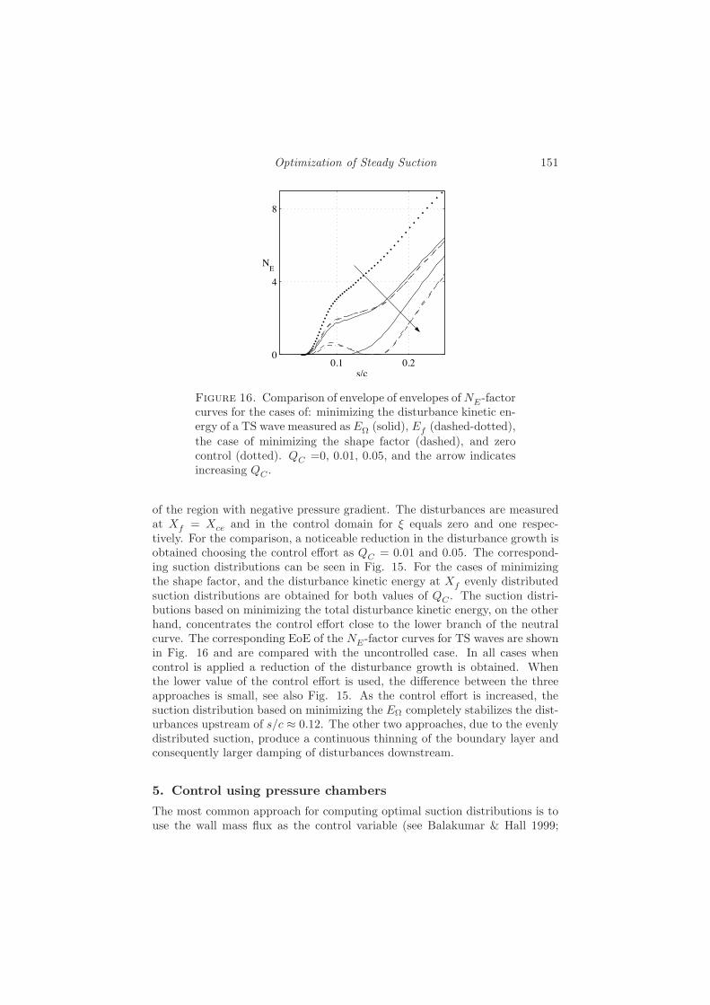
Optimization of Steady Suction 151
0.1 0.20
4
8
NE
s/c
Figure 16. Comparison of envelope of envelopes of NE-factorcurves for the cases of: minimizing the disturbance kinetic en-ergy of a TS wave measured as E! (solid), Ef (dashed-dotted),the case of minimizing the shape factor (dashed), and zerocontrol (dotted). QC =0, 0.01, 0.05, and the arrow indicatesincreasing QC .
of the region with negative pressure gradient. The disturbances are measuredat Xf = Xce and in the control domain for , equals zero and one respec-tively. For the comparison, a noticeable reduction in the disturbance growth isobtained choosing the control e!ort as QC = 0.01 and 0.05. The correspond-ing suction distributions can be seen in Fig. 15. For the cases of minimizingthe shape factor, and the disturbance kinetic energy at Xf evenly distributedsuction distributions are obtained for both values of QC . The suction distri-butions based on minimizing the total disturbance kinetic energy, on the otherhand, concentrates the control e!ort close to the lower branch of the neutralcurve. The corresponding EoE of the NE-factor curves for TS waves are shownin Fig. 16 and are compared with the uncontrolled case. In all cases whencontrol is applied a reduction of the disturbance growth is obtained. Whenthe lower value of the control e!ort is used, the di!erence between the threeapproaches is small, see also Fig. 15. As the control e!ort is increased, thesuction distribution based on minimizing the E! completely stabilizes the dist-urbances upstream of s/c * 0.12. The other two approaches, due to the evenlydistributed suction, produce a continuous thinning of the boundary layer andconsequently larger damping of disturbances downstream.
5. Control using pressure chambersThe most common approach for computing optimal suction distributions is touse the wall mass flux as the control variable (see Balakumar & Hall 1999;

152 J. O. Pralits & A. Hanifi
Airiau et al. 2003; Pralits et al. 2002). In a realistic setting, such as an ex-periment or suction systems used on wings, the suction velocity is a functionof the surface porosity, hole geometry and the pressure di!erence between thepressure distribution on the surface and static pressure in a number of discretechambers (see Reneaux & Blanchard 1992; Ellis & Poll 1996; Preist & Paluch1996; Bieler & Preist 1992; Joslin 1998). The aim here is to derive the optimalcontrol problem of Sec. 3 using the static pressures of a number of discretechambers, with fixed size and position, as control variables. We will then com-pare the results with the previously computed continuous suction distributionto assess the feasibility of the latter approach.
If a porous surface is used, then at least for flows with low free-streamvelocity, the relation between the pressure di!erence and the suction velocityis linear, in accordance with Darcy’s law. The relation between the pressuredi!erence and suction velocity used here is taken from Bieler & Preist (1992). Itis based on measurements carried out in the framework of the ELFIN (EuropeanLaminar Flow INvestigation) program. In dimensionless form this formula isgiven as
%Pj =C1
"w
m2w + C2
µw
"w
mw 0x1 ' [Xcsj, Xcej
], j = 1, · · · , K (18)
where %Pj = Pe#Pcj, in which Pe is the pressure distribution on the wing and
Pcjis the static pressure in chamber j. The first term on the right hand side of
Eq. (18) is due to the dynamic pressure loss, and the second term is the pressureloss due to skin friction. The coe"cients C1 and C2 together with a briefdescription of Eq. (18) are given in Appendix C. The choice of static pressurein the chambers is not without restrictions. The Mach number of the flowthrough the holes of the porous plate should be limited. If %Pj is too small thenblowing instead of suction might occur. Disturbances might be introduced asan e!ect of strong suction through discrete holes, which can accelerate insteadof delay laminar-turbulent transition (see Reneaux & Blanchard 1992; Ellis &Poll 1996). These restrictions are related to the design of the perforated plateand therefore not considered as constraints in the theory presented here.
5.1. Optimality system
Here a concise description of the derivation of the optimality system includingpressure chambers is given for the case of minimizing the disturbance kineticenergy. The optimal control problem is now defined as: find controls Pcj
,and states Q and q which minimize the objective function J0 given by Eq.(7) with the constraints given by Eqs. (1), (3), (4) and (8). The Lagrangemultiplier technique is also used here to enforce the constraints. The adjointvariables Q$,q$, r$,3$ and #$j where j = 1, · · · , K, are introduced and the newLagrangian functional is given as
L = J0 # J1, (19)

Optimization of Steady Suction 153
where
J1 = -Q$, LB Q.+K%
j=1
* Xcej
Xcsj
#$j8m(x1, 0)# mw
9h1dx1
+ 3$(EC #K%
j=1
* Xcej
Xcsj
m2wh1dx1) + -q$, LP q.+ -r$q,
1h1
!q!x1.+ c.c.
Compared to the previously described Lagrangian functionals, the wall bound-ary condition has now been divided into K discrete domains, and the massflux at the wall is given by Eq. (18). No additional di"culties appear in thederivation compared to the one in Sec. 3. The optimality condition is nowobtained by setting the functional derivative with respect to the static pressureof each chamber to zero. The resulting optimality system can be seen in detailin Appendix C.
5.2. Results
Here results are given for the case of minimizing the disturbance kinetic energyusing pressure chambers. The parameters in Eq. (18) which specify the poroussurface are taken from Bieler & Preist (1992). The plate thickness L andhole diameter at the surface d are 0.9 mm and 0.046 mm, respectively. Theporosity -/(4.2) is calculated given a hole pitch to diameter ratio . = 13.8. Thecoe"cients of inertial and viscous pressure loss are A = 1.6 and B = 0.092,respectively.
Before the calculations are performed, the size, position and number ofpressure chambers must be set. The di!erent sizes are chosen such that thechambers are smaller where the pressure gradient of the wing is large and viceverse. This is done to avoid large pressure drops which result in large suctionpeaks. The whole control domain (c = [Xcs, Xce] is used such that the pressurechamber closest to the leading edge starts at Xcs1
= Xcs and the last pressurechamber ends at XceK
= Xce.The results in Sec. 4.2 show that minimizing the shape factor does not
always give an optimal suction distribution which reduces the disturbancegrowth. Further, it is seen in Sec. 3.3 that both CF and TS type distur-bances should be included in the calculations when the disturbance kineticenergy is minimized. Therefore, we choose to minimize the total disturbancekinetic energy, , = 1 in Eq. (7), including both the CF and TS waves given inSec. 3.3. The control e!ort QC = 0.35 and the calculations are done for thecases of 5, 6 and 7 pressure chambers.
Results of the optimal static pressures Pcjof each case are plotted (thick
lines) in Fig. 17. The pressure distribution on the wing Pe is also plotted(thin lines) for comparison. The region s/c=[0.05,0.175] has been magnified toenhance the details. As shown, the pressure di!erence %Pj = Pe#Pcj
is largerclose to the leading edge and decreases downstream.

154 J. O. Pralits & A. Hanifi
0 0.05 0.1 0.15 0.20.4
0.8
1.2
1.6
static
pre
ssur
e
0 0.05 0.1 0.15 0.20.4
0.8
1.2
1.6
static
pre
ssur
e
0 0.05 0.1 0.15 0.20.4
0.8
1.2
1.6
static
pre
ssur
e
s/c
0.55
0.57
0.59
0.55
0.57
0.59
0.55
0.57
0.59
(a)
(b)
(c)
Figure 17. Pressure distribution on the wing (thin lines) andoptimal static pressure in the chambers (thick lines) for thecases of (a) 5; (b) 6; and (c) 7 pressure chambers minimizingthe disturbance kinetic energy E! of a CF (f$
1 = 5500 s"1,)$
1 = 2500 m"1) and TS wave (f$2 = 5750 s"1, )$
2 = 225 m"1)when QC = 0.35.
The suction distributions corresponding to the optimal static pressures inFig. 17 are plotted in Fig. 18. Note that the uppermost streamwise suctiondistribution in each case is due to the stagnation line control and is taken befixed. In each case the suction distribution downstream of s/c = 0.05 is ratherconstant. Upstream of this streamwise position the suction distributions havemore of a saw-tooth shape. The latter is an e!ect of the strong pressure gradientin this region.
For each case in Fig. 17, a comparison is made with the optimal suctiondistribution from Fig. 9 (thin lines) for the case when QC = 0.35 . As thesame control e!ort is used in these calculations, it is interesting to comparethe optimal suction distribution in a continuous control domain with the casesusing pressure chambers. It is seen that the magnitude of both the suctiondistribution from Fig. 9 and the suction distributions using pressure chambersis rather constant downstream of s/c = 0.05 and increases upstream of this

Optimization of Steady Suction 155
0 0.05 0.1 0.15 0.2−20
−15
−10
−5
0
mw
# 1
04
0 0.05 0.1 0.15 0.2−20
−15
−10
−5
0
mw
# 1
04
0 0.05 0.1 0.15 0.2−20
−15
−10
−5
0
mw
# 1
04
s/c
.
.
.
(a)
(b)
(c)
Figure 18. Suction distributions (thick lines) correspondingto the optimal pressure drop for the cases of (a) 5; (b) 6; and(c) 7 pressure chambers in figure 17. A comparison is donewith the optimal suction distribution (thin lines) from figure9 when QC = 0.35.
position. Further, the distribution using pressure chambers approaches thecontinuous one when the number of chambers is increased. This is most evidentdownstream of s/c = 0.05.
The e!ect on the disturbance growth using the optimal pressure di!erencesfor the cases of 5, 6 and 7 pressure chambers is shown in Fig. 19. Here the EoEof the NE-factor curves for CF and TS waves are plotted for zero and optimalpressure di!erences of all cases (solid lines). The arrows mark the directionof increasing number of pressure chambers. A decrease in the growth of bothCF and TS waves is obtained for all optimal pressure di!erences calculatedhere compared to the case of zero suction. The CF waves are more dampedin the control domain when the number of pressure chambers is increased.However, the di!erence between the cases of having 6 and 7 pressure chambersis small as the additional chamber is placed where the CF waves begin todecay. The results for the TS waves show that upstream of s/c = 0.1, the EoEcurves increase in magnitude as the number of pressure chambers increases.

156 J. O. Pralits & A. Hanifi
0 0.1 0.2 0.3 0.4 0.50
4
8
12
16
20
NE
s/c
CF
TS
Figure 19. Envelope of envelopes (EoE) of NE-factor curvesfor the disturbances given in table 1 for the cases of zero con-trol (dotted) and the optimal pressure chambers in figure 17(solid). The arrows mark increasing number of pressure cham-bers. A comparison is done with the EoE of NE-factor curves(dashed) from figure 11 with QC = 0.35.
Downstream of this position EoE curves decrease in magnitude. A comparisonis made with the EoE of the NE-factor curves in Fig. 11 which are calculatedusing the suction distribution from Fig. 9 with QC = 0.35 (dashed lines). It isseen that as the number of pressure chambers are increased, the results withinthe control domain using pressure chambers approach those using a suctiondistribution in a continuous control domain. This is true for the results of boththe CF and TS waves.
6. Discussion and conclusionsA method to control convectively unstable disturbances in boundary layers oninfinite swept wings for compressible fluids has been derived and analyzed. Themethod has been developed in the framework of optimal control theory. Themean of disturbance control is a modification of the mean flow by the mass flowthrough a porous surface. The optimization problem is derived using Lagrangemultipliers from which optimality systems are obtained containing the adjointof the parabolized stability equations (APSE) and the adjoint of the boundarylayer equations (ABLE).
Two di!erent control variables are considered. The first control variableis the mass flow at the wall. Here, it is assumed that given a certain controldomain, the suction distribution is not constrained by how it will be imple-mented on the wing and thus has the optimal distribution with respect to acertain objective function. The second control variable is the static pressure ina number of pressure chambers. Here, the suction velocity is a function of the

Optimization of Steady Suction 157
surface porosity, hole geometry and the pressure di!erence between the pres-sure distribution on the wing and the internal static pressure of the pressurechambers. In this case, the internal static pressure of each box is optimized.In both cases, the control e!ort has not been regularized, but instead enforcedas a constraint.
Di!erent measures of the state (objective functions) have been analyzed.The first objective function is a measure of the disturbance kinetic energy. Acomparison has been made between minimizing the kinetic energy of a singledisturbance at a fixed streamwise position, and minimizing the streamwiseintegral of the kinetic energy of an arbitrary number of disturbances. Forcontrol of a single CF wave, the di!erence between the two objective functionsis small. The advantage of the latter is that more than one disturbance canbe included in the measure. On the wing studied here, both cross flow and TSwaves are amplified on the upstream part. Results show that both disturbancetypes need to be accounted for in the objective function in order for the controlto decrease their growth. Further, it is su"cient to account for one of eachdisturbance type in order to control all other disturbances of the same type.
The second measure of the state used here is the streamwise integral of theshape factor, H12. Airiau et al. (2003) showed that this quantity is successfulfor control of two-dimensional disturbances in Blasius flow. In terms of com-putational e!ort, the approach of minimizing the shape factor is e"cient. Theoptimality condition for each iteration in the optimization process is obtainedafter solving the boundary layer and corresponding adjoint equation once. Thedisadvantage lies in the fact that one does not take into account the disturbancegrowth in the optimization process, and consequently the e!ect of the controlon the disturbance growth needs to be analyzed afterwards. Results here showthat a control based on this objective function amplify instead of damp cross-flow modes in the region close to the leading edge of the wing. In this region,the optimal mass-flow distribution has a positive sign i. e. blowing occurs. Theamplification of disturbances mean that the point of laminar-turbulent tran-sition will move upstream and the laminar portion of the wing will decrease.Further, as the current way of implementing suction systems relies on pressurechambers, a region of blowing is not realizable.
Results are also presented for the optimal static pressure in a number ofpressure chambers. These results depend on the choice of size, position andnumber of the chambers. However, it can be shown that the correspondingsuction distributions are similar in magnitude compared to the result of theoptimal suction distribution in a continuous control domain. This similarityincreases as the number of pressure chambers is increased.
The magnitudes of the suction distributions presented in this paper are allof order O(Re"1), which is within the range of validity of the boundary-layerequations. As Airiau et al. (2003) showed, for the suction rate of this order, theboundary-layer and Navier-Stokes calculations agreed well though the optimalmass flux experiences locally large streamwise variation.

158 J. O. Pralits & A. Hanifi
7. AcknowledgmentThe useful discussion with C. Airiau and other colleagues, and financial sup-port of the EU project (ALTTA contract G4RD-CT-2000-00143) is gratefullyacknowledged.
Appendix A. Optimal control using the wall mass flux tominimize the disturbance kinetic energy
A.1. State equations
The boundary-layer equations for a viscous compressible flow over a swept wingwith an infinite span are
1h1
!("U)!x1
+!("W )!x3
= 0, (20)
"U
h1
!U
!x1+ "W
!U
!x3= # 1
h1
dPe
dx1+
1Re
!
!x3
-µ!U
!x3
., (21)
"U
h1
!V
!x1+ "W
!V
!x3=
1Re
!
!x3
-µ!V
!x3
., (22)
cp"U
h1
!T
!x1+ cp"W
!T
!x3=
1RePr
!
!x3
-$!T
!x3
.+
(% # 1)UM2
h1
dPe
dx1+ (% # 1)
µM2
Re
C-!U
!x3
.2
+-!V
!x3
.2D
. (23)
The parabolized stability equations are lengthy and here are given in a symbolicform
Aq + B !q!x3
+ C !2q(!x3)2
+ D 1h1
!q!x1
= 0, (24)
* +#
0qH !q!x1
dx3 = 0, 0x1 ' [X0, X1], (25)
where q = (", u, v, w, T )T. The coe"cients of the 5( 5 matrices A,B, C and Dare found in Pralits et al. (2000). The corresponding boundary conditions are
W (x1, 0) = Ww(x1) 0x1 ' (c,
W (x1, 0) = 0 0x1 /' (c,/U, V,
!T
!x3
0(x1, 0) = [0, 0, 0] 0x1 ' [XS , X1],
limx3%+#
[U, V, T ] (x1, x3) = [Ue, Ve, Te] (x1) 0x1 ' [XS , X1],!u, v, w, T
"(x1, 0) = [0, 0, 0, 0] 0x1 ' [X0, X1],
limx3%+#
!u, v, w, T
"(x1, x3) = [0, 0, 0, 0] 0x1 ' [X0, X1],

Optimization of Steady Suction 159
where variables with subscript w are evaluated at the wall, and subscript e atthe boundary layer edge. The initial conditions are
Q(XS , x3) = QS(x3) 0x3 ' [0, +&),q(X0, x
3) = q0(x3) 0x3 ' [0, +&),
where the solution of variables with subscript 0 is given by the local stabilityanalysis, and subscript S by the solution at the stagnation line.
A.2. Adjoint equations
The adjoint of the boundary-layer equations are
"!(h1W
$)!x3
# h1"
-!U
!x3U$ +
!V
!x3V $ + cp
!T
!x3T $.
= FW h1, (26)
!("UU$)!x1
+!(h1"WU$)
!x3# "
-!U
!x1U$ +
!V
!x1V $ # !W $
!x1+ cp
!T
!x1T $.
+
(% # 1)M2 dPe
dx1T $ # 2(% # 1)
ReM2 !
!x3
-h1µ
!U
!x3T $.
+
1Re
!
!x3
-µ!(h1U
$)!x3
.= FU h1, (27)
!("UV $)!x1
+!(h1"WV $)
!x3# 2(% # 1)
ReM2 !
!x3
-h1µ
!V
!x3T $.
+
1Re
!
!x3
-µ!(h1V
$)!x3
.= FV h1, (28)
cp!("UT $)!x1
+ cp!(h1"WT $)
!x3+"U
T
-!U
!x1U$ +
!V
!x1V $ # !W $
!x1
.+
"U
Tcp!T
!x1T $ +
$
RePr!2(h1T
$)(!x3)2
(% # 1)Re
M2 dµ
dT
C-!U
!x3
.2
+-!V
!x3
.2D
T $ #
1Re
dµ
dT
/!U
!x3
!(h1U$)
!x3+!V
!x3
!(h1V$)
!x3
0= FEh1, (29)
where FE = (FT + FW W/T )h1, and FW , FU , FV , FT are found in Pralits(2001). The adjoint of the parabolized stability equations can be written as
Aq$ + B !q$
!x3+ C !2q$
(!x3)2+ D 1
h1
!q$
!x1= S$
P, (30)
!
!x1
* +#
0q$H
-!A!(
+!B!(
.q h1dx3 =
@A
B
0 0x1 /' [Xms, Xme],
#i|$|2* +#
0qHM q h1dx3 0x1 ' [Xms, Xme],
(31)

160 J. O. Pralits & A. Hanifi
where
S$P =
@EA
EB
#r$!q!x1# !(r$q)
!x10x1 /' [Xms, Xme],
#r$!q!x1# !(r$q)
!x1+ ,MHq|$|2 0x1 ' [Xms, Xme],
and
A = AH # !BH
!x3# m13 BH +
!2CH
(!x3)2+ 2 m13
!CH
!x3# !DH
!x1,
B = #BH + 2!CH
!x3+ 2 m13 CH,
C = CH,
D = #DH.
The vector q$ = ("$, u$, v$, w$, '$)T, and the complete derivation of theseequations is found in Pralits et al. (2000). The above equations are subjectedto the following boundary conditions
[u$, v$, w$, '$] (x1, 0) = [0, 0, 0, 0] 0x1 ' [X0, X1],lim
x3%+#[u$, v$, w$, '$] (x1, x3) = [0, 0, 0, 0] 0x1 ' [X0, X1],
[U$, V $] (x1, 0) = [0, 0] 0x1 ' [X0, X1],/
$
RePr!(h1T
$)!x3
+ h1"cpWT $0
(x1, 0) = 0 0x1 ' [X0, X1],
limx3%+#
[U$, V $, W $, T $] (x1, x3) = [0, 0, 0, 0] 0x1 ' [X0, X1].
The initial conditions areq$(X1, x
3) = (1# ,)q$1(x3) 0x3 ' [0, +&),
r$(X1) = (1# ,)r$1 0x3 ' [0, +&),Q$(X1, x
3) = 0 0x3 ' [0, +&),
with q$1 and r$1 evaluated at x1 = X1 as
q$1 = |$|2D+(M # c1I)q, r$1 = |$|2 c1,
c1 =
* #
0(h1qHM D+H
-!A!(
+!B!(
.q# iqHM q) dx3
* #
0qHD+H
-!A!(
+!B!(
.q h1 dx3
,(32)
where D+ = (DH)"1.
A.3. Optimality condition
The optimality condition is
W $w =
6#23$mw 0x1 ' (c,
0 0x1 /' (c,(33)

Optimization of Steady Suction 161
where
3$ =
+1
4EC
* Xce
Xcs
W $2w h1dx1
, 12
.
Appendix B. Optimal control using the wall mass flux tominimize the shape factor
B.1. State equations
The boundary layer equations are given by Eqs. (20), (21), (22) and (23) withcorresponding boundary and initial conditions as given in A.1.
B.2. Adjoint equations
The adjoint boundary layer equations are given by Eqs. (26), (27), (28) and(29) where the component of the forcing S$
B = (FW , FU , FV , FE) are now
FW = 0, FU =102" cos(5)(1 + H12(1# 2USL))
Ue0
Qe,
FV =102" sin(5)(1+H12(1#2USL))
Ue0
Qe, FE = # 1
02
"
TUSL(1+H12(1#USL))
Te0
Te,
The initial and boundary conditions are the ones given in A.2, except forfreestream boundary conditions which are now given as
limx3%+#
/!U$
!x3,!V $
!x3, W $,
!T $
!x3
0(x1, x3) = [0, 0, 0, 0] 0x1 ' [X0, X1].
B.3. Optimality condition
The optimality condition is given by Eq. (33).
Appendix C. Optimal control using pressure chambers tominimize the disturbance kinetic energy
C.1. Relation between internal static pressure and mass flux
The relation between the pressure di!erence and suction velocity used here istaken from Bieler & Preist (1992). It is based on measurements carried out inthe framework of the ELFIN (European Laminar Flow INvestigation) program.In dimensionless form this formula is given as
%Pj = Pe # Pcj=
C1
"w
m2w + C2
µw
"w
mw
where
C1 =A
2
-4.2
-
.2
, C2 =32B
Re4.2
-
L
d2.
The porous plate has a thickness L and a hole diameter d at the surface.Due to manufacturing reasons the holes were slightly conical with an inner

162 J. O. Pralits & A. Hanifi
diameter D. The porosity is given as -/(4.2), where . is the ratio between thehole diameter on the surface and the distance between the holes.
It was found in experiments that the relationship between the suction ve-locity and pressure di!erence was non-linear and that adding a term due todynamic pressure loss with an empirically obtained coe"cient A gave a goodagreement with experiments (see Bieler & Preist 1992). The second term onthe right hand side of the formula is based on the Hagen-Poiseuille equation forpressure loss due to skin friction in a hole with parallel walls. The coe"cientB is a function of the inner and outer hole diameters and serves as a correctiondue to the conical shape of the holes.
C.2. State equations
The boundary-layer equations are given by Eqs. (20), (21), (22) and (23) withcorresponding initial conditions as given in A.1. All boundary conditions arethe same as given in A.1, except for the wall normal mean velocity at the wall,which is now given by
W (x1, 0) =
@EA
EB
0 0x1 /' [Xcsj, Xcej
],
#12
C2
C1
µw
"w+
#-12
C2
C1
µw
"w
.2
+ %Pj
"w
C1
0x1 ' [Xcsj, Xcej
].
The values used here for A, B, L, d and . are taken from Bieler & Preist (1992).The parabolized stability equations are given by Eqs. (24) and (25) with cor-responding boundary and initial conditions as given in A.1.
C.3. Adjoint equations
The adjoint parabolized stability equations are given by Eqs. (30) and (31) withcorresponding boundary and initial conditions as given in A.1. The adjointboundary layer equations are given by Eqs. (26), (27), (28) and (29) withcorresponding initial conditions as given in A.2. All boundary conditions arethe same as given in A.2, except for T $ at the wall, which is now given by/
$
RePr!(h1T
$)!x3
+ h1"cpWT $0(x1, 0) =
20 0x1 /' [Xcsj
, Xcej],
Kj(W $+ 23$mw) 0x1' [Xcsj, Xcej
],
where
Kj =!Pcj
!Tw
/!Pcj
!mw
,
and!Pcj
!Tw=
1"wTw
C1m2w + C2
1"w
-µw
Tw+
dµw
dTw
.mw
!Pcj
!mw=
2C1
"wmw + C2
µw
"w
FEEEG
EEEH0x1 ' [Xcsj
, Xcej].

Optimization of Steady Suction 163
C.4. Optimality condition
#* Xcej
Xcsj
(W $w + 23$mw)
+!Pcj
!mw
,"1
h1dx1 = 0, j = 1, · · · , K.
where
3$ =
I
J 14EC
K%
j=1
* Xcej
Xcsj
W $2w h1dx1
K
L
12
.
References
Airiau, C., Bottaro, A., Walther, S. & Legendre, D. 2003 A methodology foroptimal laminar flow control: Application to the damping of tollmien-schlichtingwaves in a boundary layer. Phys. Fluids 15, 1131–1145.
Atkin, C. 2000 New aerodynamic approach to suction system design. InCEAS/DragNet European Drag Reduction Conference (ed. P. Thiede). Potsdam,Germany: Springer.
Balakumar, P. & Hall, P. 1999 Optimum suction distribution for transition pre-diction. Theor. Comput. Fluid Dyn. 13, 1–19.
Bertolotti, F., Herbert, T. & Spalart, S. 1992 Linear and nonlinear stabilityof the blasius boundary layer. J. Fluid Mech. 242, 441–474.
Bewley, T. 2001 Flow control: new challenges for a new renaissance. Progess inAerospace Sciences 37, 21–58.
Bieler, H. & Preist, J. 1992 Hlfc for commercial aircraft. In First european forumon laminar flow technology , pp. 193–199. Hamburg.
Byrd, R., Lu, P., Nocedal, J. & Zhu, C. 1995 A limited memory algorithm forbound constrained optimization. SIAM J. Sci. Comput. 16, 1190–1208.
Cathalifaud, P. & Luchini, P. 2000 Algebraic growth in a boundary layer: optimalcontrol by blowing and suction at the wall. Eur. J. Mech. B/Fluids 19 (4), 469–490.
Ellis, J. & Poll, D. 1996 Laminar and laminarizing boundary layers by suctionthrough perforated plates. In Second european forum on laminar flow technology ,pp. 8.17–8.26. Bordeaux.
Gunzburger, M. D. 1997 Introduction into mathematical aspects of flow controland optimization, von karman institute for fluid dynamics, lecture series 1997-05. Inverse Design and Optimization Methods .
Hanifi, A., Henningson, D. S., Hein, S. & Bertolotti, F. P.and Simen, M.1994 Linear non-local instability analysis - the linear nolot code. FFA TN 1994-54.
Hanifi, A., Schmid, P. J. & Henningson, D. S. 1996 Transient growth in com-pressible boundary layer flow. Phys. Fluids 8 (3), 826–837.
Herbert, T. 1997 Parabolized stability equations. Annu. Rev. Fluid Mech. 29, 245–283.
Hill, D. C. 1997b Inverse design for laminar three-dimensional boundary layers.Bull. Am. Phys. Soc. 42, 2120.

164 References
Hogberg, M. & Henningson, D. S. 2001 Linear optimal control applied to insta-bilities in spatial boundary layers. J. Fluid Mech. Submitted.
van Ingen, J. L. 1956 A suggested semiempirical method for the calculation of theboundary layer transition region. Tech. Rep. VTH-74. Department of Aeronau-tical Engineering, University of Delft.
Joslin, R. 1998 Overview of laminar flow control. Tech. Rep. 1998-208705. NASA,Langley Research Center, Hampton, Virginia.
Malik, M. R. & Balakumar, P. 1992 Nonparallel stability of rotating disk flowusing pse. In Instability, Transition and Turbulence (eds. M. Hussaini, A. Kumar& C. Streett), pp. 168–180. Springer.
Mughal, M. 1998 Active control of instabilities in three-dimensional compressibleflows. Theor. Comput. Fluid Dyn. 12, 195–217.
Pralits, J. O. 2001 Towards optimal design of vehicles with low drag: Applicationsto sensitivity analysis and optimal control. Licentiate thesis KTH/MEK/TR-01/07. Royal Institute of Technology, SE-172 90 Stockholm, Sweden.
Pralits, J. O., Airiau, C., Hanifi, A. & Henningson, D. S. 2000 Sensitivity anal-ysis using adjoint parabolized stability equations for compressible flows. Flow,Turbulence and Combustion 65, 321–346.
Pralits, J. O., Hanifi, A. & Henningson, D. S. 2002 Adjoint-based optimizationof steady suction for disturbance control in incompressible flows. J. Fluid Mech.467, 129–161.
Preist, K. & Paluch, B. 1996 Design specification and inspection of perforatedpanels for hlf suction systems. In Second european forum on laminar flow tech-nology , pp. 6.20–6.34. Bordeaux.
Reneaux, J. & Blanchard, A. 1992 The design and testing of an airfoil with hybridlaminar flow control. In First european forum on laminar flow technology , pp.164–174. Hamburg.
Schlichting, H. 1943/44 Die beeinflussung der grenzschicht durch absaugung undausblasen. Jb. dt. Adad. d. Luftfahrtforschung 90-108.
Simen, M. 1992 Local and non-local stability theory of spatially varying flows. In In-stability, Transition and Turbulence (eds. M. Hussaini, A. Kumar & C. Streett),pp. 181–201. Springer.
Smith, A. M. O. & Gamberoni, N. 1956 Transition, pressure gradient and stabilitytheory. Tech. Rep. ES 26388. Douglas Aircraft Co.
Walther, S., Airiau, C. & Bottaro, A. 2001 Optimal control of tollmien-schlichting waves in a developing boundary layer. Phys. Fluids 13, 2087–2096.
Zhu, C., Byrd, R., Lu, P. & Nocedal, J. 1994 L-bfgs-b: Fortran subroutines forlarge scale bound constrained optimization. Tech. Rep. NAM-11. EECS Depart-ment, Northwestern University.

Paper 4
4


Optimization of Steady Wall Temperature forDisturbance Control
By Jan O. Pralits1,2 and Ardeshir Hanifi2
We present a theory for computing the optimal steady wall temperature dis-tribution to suppress the growth of convectively unstable disturbances in com-pressible boundary layer flows on flat plates. A gradient based iterative pro-cedure is used to minimize an objective function measuring the disturbancekinetic energy. The gradient of interest is obtained from the solution of theadjoint of the boundary layer and parabolized stability equations, which arederived using a Lagrange multiplier technique. The study includes a compar-ison between the cases of minimizing the terminal, and an integrated value ofthe disturbance kinetic energy for di!erent freestream Mach numbers and con-trol magnitudes. A comparison is also made for the cases of zero and non-zerowall heat transfer outside the control domain.
1. IntroductionDelay of laminar-turbulent transition is desired in a number of applications. Itwas early recognized that uniformly distributed cooling has a damping e!ecton viscous instabilities for various Mach number flows, see e. g. experimentsby Diaconis et al. (1957) and Jack et al. (1957). Liepmann & Fila (1947),showed that at low subsonic speeds the transition location moves upstream ona heated flat plate. The destabilizing e!ect of heating is due to the increaseof the viscosity of air close to the wall, which creates inflectional velocity pro-files there. Cooling the wall on the other hand, decreases the viscosity nearthe wall which results in a thicker velocity profile and thus a more stable flow.Lees & Lin (1946) using inviscid theory and Mack (1984) using viscous theoryfound that subsonic air boundary layers can be completely stabilized by uni-formly distributed wall-cooling. Mack also showed that uniformly distributedwall-cooling has a destabilizing e!ect on the higher modes (also known as theMack modes) which appear at high Mach numbers. His results for supersonicflows have been experimentally verified by Lysenko & Maslov (1984). Masadet al. (1992) reported similar results using the spatial stability equations forcompressible flows.
1Department of Mechanics, KTH, SE-100 44 Stockholm, Sweden.2Swedish Defence Research Agency, FOI, Aeronautics Division, FFA, SE-172 90 Stockholm,Sweden.
167

168 J. O. Pralits & A. Hanifi
More recent studies by Masad & Nayfeh (1992) and Lo et al. (1995), haveshown that discrete heating strips located upstream of the first neutral pointdecreases the maximum amplification of disturbances in subsonic boundarylayers. As the heating strip is moved downstream, into the unstable region,the maximum amplification is increased. The opposite was found for discretecooling strips which was explained to be due to the fact that the flow whichleaves the cooled domain experiences a relatively hotter surface downstream.Massad & Nayfeh used also the interactive boundary-layer theory to account forthe pressure gradient induced by thickening/thinning of boundary layer due toheating/cooling strips. However, they concluded that the di!erences betweenthe N -factors using the mean flow obtained from interactive, and non-similarboundary layer equations are small.
In the most of the works found in the literature, the e!ects of wall-coolingor -heating on disturbance growth are studied using a predefined temperaturedistribution in either a continuous or discrete domain (strips). However, insome earlier works by other researchers, the problem of temperature optimiza-tion has been addressed. In Masad & Nayfeh (1992), a parameter study wasperformed in order to find the best location for a heating strip with a givenlength and a constant ratio between the wall and adiabatic temperature. InGunzburger et al. (1993) an optimal control problem using boundary controlsfor the incompressible Navier-Stokes equations was derived. An application ofcontrol by heating and cooling was given with the wall heat flux as the controlparameter and a target wall temperature as the objective. However, in noneof these works an optimal temperature distribution in terms of minimizing ameasure of disturbance amplitude has been derived. In Hill (1997b), an inversemethod to compute the optimal cooling/heating distributions was mentionedbut no details were given there.
In this paper, we present the theory and examples of optimal distributionof temperature in discrete domains which minimize the growth of connectivelyunstable disturbances in a growing boundary layer. The evolution of thesedisturbances in a quasi three-dimensional boundary layer is here analyzed usingthe Parabolized Stability Equations (PSE) (see Bertolotti et al. 1992; Simen1992; Malik & Balakumar 1992; Herbert 1997) derived for compressible flows,see section 2. The control problem is defined in section 3 using optimal controltheory in which a Lagrange multiplier technique is used. The aim is to minimizesome measure of the disturbance amplitude for a given cooling/heating energy.The optimality systems consists of solving state and corresponding adjointequations from which an optimality condition is evaluated. Here, we couplethe adjoint of the PSE with the adjoint of the boundary-layer equations inorder to find the optimality condition.
In section 5 results are presented for optimal temperature distribution tocontrol disturbance growth in flat plate boundary-layer flows. Here, the e!ectsof the control magnitude, objective function, Mach number and heat transfer

Optimization of temperature 169
outside the control domain are investigated. The summary and conclusions aregiven in section 6.
2. State equationsThe flow field is given by the solution of the mass, momentum and energy con-servation equations for a viscous compressible flow. The equations are writtenfor Cartesian coordinates with streamwise, spanwise and wall-normal coordi-nates denoted as x1, x2 and x3 respectively. The total flow field, qtot is decom-posed into a mean, q, and a perturbation part, q, as
qtot(x1, x2, x3, t) = q(x1, x3) + q(x1, x2, x3, t)
where q ' [U, V, W, P, T, "] and q ' [u, v, w, p, T , "]. Here U, V, W are thestreamwise, spanwise and wall-normal velocity components of the mean flowrespectively, T is the temperature, " the density and P the pressure. Therespective lower case variables correspond to the disturbance quantities. Themean flow has zero variation in the spanwise direction and the evolution ofconvectively unstable disturbances is analyzed in the frame-work of the nonlocalstability theory. The mean flow and disturbance equations in the followingsections are given in dimensionless form. All flow and material quantities aremade dimensionless with the corresponding reference flow quantities at a fixedstreamwise position x!
0, except the pressure, which is referred to twice thecorresponding dynamic pressure. Here, dimensional quantities are denoted bythe superscript 4.
The reference length scale is taken as l!0 = (&!0x!
0/U!0 ) 1
2 . The Reynoldsand Mach number are defined as Re0 = l!0U
!0 /&!
0 and M = U!0 /(R%T !
0 ) 12 re-
spectively where R is the specific gas constant, & the kinematic viscosity and% the ratio of specific heats. The dynamic viscosity is calculated using theSutherland law. The coe"cient of the specific heat cp and the thermal conduc-tivity $ are both functions of temperature as 4th order polynomials fitted toa set of experimental data. The bulk viscosity is calculated using the formulagiven by Bertolotti (1998) and the Prandtl number is calculated based on thereference temperature, see Appendix B.
2.1. Mean Flow equations and control variable
The dimensionless boundary layer equations (BLE) written in the primitivevariables form can be found in Appendix A. These are here written in symbolicform as
LB Q = 0 (1)where Q = (U, V, W, T )T. The velocity components are zero at the wall and theheated or cooled plate is defined by T (x1, 0) = Tw(x1) in a streamwise domain(C = [Xcs, Xce]. Here, subscripts cs and ce refers to the start and end of thecontrol domain, respectively. As the control Tw(x1) is not applied along thewhole plate, it is necessary to define the boundary condition of the temperatureupstream and downstream of (C. Here, two di!erent choices of boundary

170 J. O. Pralits & A. Hanifi
conditions are considered outside of the control domain. In the first, denotedTW1, the wall temperature is prescribed as T (x1, 0) = Tw0
. Here Tw0can be for
instance the adiabatic wall temperature for the uncontrolled case. The secondchoice for boundary condition, denoted TW2, is to set !T (x1, 0)/!x3 = 0outside of the control domain. The e!ects on the mean flow due to the choiceof boundary condition will appear as cooling or heating is applied. However,due to the parabolic nature of the BLE, only the mean flow in the domaindownstream of (C will change. If TW1 is chosen then as the control is applied,the flow downstream of (C will no longer satisfy !T (x1, 0)/!x3 = 0, i. e. the wallis no longer considered to be adiabatic. If TW2 is chosen then as the control isapplied, the wall temperature will change in order to satisfy the adiabatic wallboundary condition. Note that we here assume that the freestream velocitydoes not change as the control is applied. If the temperature distributionwould result in a large change in the boundary layer thickness, then it may benecessary to update the freestream velocity in the optimization process.
2.2. Disturbance equations
The perturbations are assumed to be time and spanwise periodic disturbancesas
q(xi, t) = q(x1, x3)$ where $ = exp
+i* x1
X0
((x!)dx! + i)x2 # i*t
,, (2)
where ( is the complex streamwise wavenumber, ) the real spanwise wavenum-ber and * the real disturbance angular frequency. The initial streamwise po-sition where the disturbances are superimposed on the mean flow is denotedX0. We assume a scale separation Re"1 between the weak variation in thex1-direction and the strong variation in the x3-direction. Further, it is as-sumed that !/!x1 4 O(Re"1) and W 4 O(Re"1). Introducing Eq. (2) andthe assumptions above in the linearized governing equations, keeping termsup to order O(Re"1), yield a set of nearly parabolic partial di!erential equa-tions (see Bertolotti et al. 1992; Malik & Balakumar 1992; Simen 1992; Herbert1997). A complete description of the equations and corresponding numericalschemes used here are given in Hanifi et al. (1994) and Hein et al. (1994). Thesystem of equations, denoted parabolized stability equations (PSE) are givenin Appendix A and are here written in symbolic form as
LP q = 0 (3)
where q = (", u, v, w, T )T. The variables u, v, w and T are subject to Dirich-let boundary conditions. To remove the ambiguity of having x1-dependenceof both the amplitude and the wave function in Eq. (2) and to maintain aslow streamwise variation of the amplitude function q, a so called ’auxiliarycondition’ is introduced
* +#
0qH !q!x1
dx3 = 0, (4)

Optimization of temperature 171
where superscript H refers to the complex conjugate transpose. Equation (3)is integrated in the downstream direction with an initial condition given bythe local stability theory at x1 = X0. At each x1-position the streamwisewavenumber ( is iterated such that Eq. (4) is satisfied. When a convergedstreamwise wavenumber has been obtained, the growth rate can be calculatedfrom the following relation
+E = #(i +!
!x1(ln)
E)
where
E =* +#
0" (|u|2 + |v|2 + |w|2) dx3,
is the kinetic energy based on the amplitude functions of the disturbance ve-locity components. The growth rate can then be used to predict the transitionlocation using the so called eN -method (see van Ingen 1956; Smith & Gam-beroni 1956). The N -factor based on the disturbance kinetic energy NE is heredefined as
NE =* x1
Xn1
+E dx1,
where Xn1 is the first neutral point (+E = 0).
3. Disturbance controlThe approach of the current work is to use optimal control theory to find theoptimal mean wall-temperature distribution in order to suppress the growth ofconvectively unstable disturbances. The problem consists of the state variablesQ and q; a control variable given by the temperature at the wall; constraints onthe state variables given by the BLE and PSE; and a cost function, a measureof the state, to be minimized.
The final goal of cooling or heating the plate is to increase the laminarportion i. e. to move the location of the laminar-turbulent transition furtherdownstream, and thus decrease the viscous drag. It is therefore important thatthe chosen cost function can be related to the transition process. One choice isto measure the kinetic energy of a certain disturbance at a given downstreamposition, say Xf . This can be written as
Ef =12
* Z1
Z0
* +#
0qHM q dx2dx3
11111x1=Xf
, (5)
where M = diag(0, 1, 1, 1, 0) which means that the disturbance kinetic energyis calculated from the disturbance velocity components. If the position Xfis chosen as the upper branch of the neutral curve, then the measure can be

172 J. O. Pralits & A. Hanifi
related to the maximum value of the N -factor of a given disturbance as
Nmax = ln
#Ef
E0
, (6)
where E0 is the disturbance kinetic energy at the first neutral point. If inaddition the measured disturbance is the one which first (with zero control)reaches the transition N -factor, then Xf can be related to the onset of thelaminar-turbulent transition. It is however not clear, a priori, that minimizingsuch a measure will damp the chosen disturbance in the whole unstable region.If the optimal control only acts close to the position of the measurement thena situation might occur where the amplification of the disturbance upstream ofthis position is still large enough to cause transition. We also have to considerthat many di!erent instability waves simultaneously exist inside the boundarylayer. Even though the one which first causes transition in the uncontrolled caseis chosen to compute Ef , it is not certain that the resulting optimal temperaturedistribution will have a damping e!ect also on other waves. For computationof optimal suction distributions in Blasius flow, it has been shown that a costfunction based on a single TS wave is su"cient to successfully damp the growthof other TS waves (see Pralits et al. 2002; Airiau et al. 2003). There are howeverother situations, such as the boundary layer flow on infinite swept wings, whereit is common that both TS and cross-flow waves are present. As these wavesare amplified in di!erent streamwise regions due to the streamwise variation ofthe mean flow pressure gradient, an optimal control based on minimizing e. g.a TS wave does not necessarily have a damping e!ect on the cross flow waves.See Pralits & Hanifi (2003) for such results regarding optimization of mean flowsuction distributions. An alternative is therefore to measure the kinetic energyas the streamwise integral over a defined domain. Using such an approach,several di!erent disturbances having their maximum growth rate at di!erentpositions, can be accounted for in one and the same optimization. Here, thesize of K disturbances superimposed on the mean flow at an upstream positionX0, is measured by their total kinetic energy as
E! =K%
k=1
12
* Xme
Xms
* Z1
Z0
* +#
0qH
kM qk dx1dx2dx3, (7)
where Xms and Xme refer to start and end positions of the measuring domain.We now define the objective function based on the disturbance growth as
J0 = ,E! + (1# ,)Ef , (8)
where the parameter , can have values between zero or one, depending on thequantity one wants to minimize.
If no restriction is given on the magnitude of the wall temperature thenthe cooling level is bounded by T (x1, 0) = 0 and in terms of heating, the walltemperature is unbounded. We therefore define a dimensionless measure of the

Optimization of temperature 173
control e!ort as
EC =E$
C
T $20
=* Xce
Xcs
&Tw # Tad0
(x1, 0)'2
dx1, (9)
where E$C is the dimensional value of the control e!ort. With expression (9) we
can compare control at di!erent Mach numbers for a fixed value of E$C. Equa-
tion (9) expresses the deviation of the control from the zero control state. Here,the zero control case corresponds to adiabatic wall temperature, Tad0
(x1, 0), i.e. the wall temperature satisfying !T/!x3(x1, 0) = 0 when no cooling or heat-ing is applied. At each streamwise position, the amplitude of the control canbe expressed as %T = Tw # Tad0
(x1, 0). In order to account for both coolingand heating, we take the square of %T .
A concise description of the objective can now be made: find the controlTw, and corresponding states Q and q which minimizes the objective functionJ0 with the constraints given by Eqs. (1), (3), (4) and (9). We now usea Lagrange multiplier technique to replace the original constrained problemwith an unconstrained one, see e. g. Gunzburger (1997). In order to enforcethe constraints we introduce the adjoint variables Q$,q$, r$,#$,3$ and theLagrangian functional
L = J0 # J1 (10)where
J1 = -Q$, LB Q.+* Xce
Xcs
#$8T (x1, 0)# Tw
9dx1
+ 3$(EC #* Xce
Xcs
&Tw # Tad0
(x1, 0)'2
dx1)
+ -q$, LP q.+ -r$q,!q!x1.+ c.c.
and c.c. denotes the complex conjugate. The inner products -·, ·. appearingabove are defined as
-/,5. =* X1
X0
* Z1
Z0
* +#
0/H5 dx1dx2dx3, (11)
for complex valued vectors / and 5. We can now define the problem as: findthe control Tw, state variables Q, q and adjoint variables #$,3$,Q$,q$ andr$ such that L is rendered stationary according to the first-order necessarycondition for an extremal point. This is done by setting the first variationof L with respect to the variables considered here to zero, while each of L’sarguments are considered to be independent variables. This requirement comesfrom the fact that at an extremal point the first variation of L with respect toeach variable vanishes. We start by setting the first variation of L with respectto each of the adjoint variables to zero, which gives the state equations (1),(3) and (4), and the constraint on the control e!ort, Eq. (9). We continue bysetting the first variation of L with respect to the state variables q, ( and Q

174 J. O. Pralits & A. Hanifi
to zero. After a procedure which involves successive integrations by parts (seePralits et al. 2002), this yields the adjoint equations
L$P q$ = S$
P, (12)
!
!x1
* +#
0q$H !LP
!(qh1dx3 =
@A
B
0 0x1 /' [Xms, Xme]
#i|$|2* +#
0qHM qh1dx3 0x1 ' [Xms, Xme],
(13)L$
B Q$ = S$B, (14)
where q$ = ("$, u$, v$, w$, '$)T and Q$ = (U$, V $, W $,T $)T. Equation (12) isthe adjoint of the PSE (APSE) where u$, v$, w$ and '$ are subject to Dirichletboundary conditions. The right hand side S$
P is due to the auxiliary condition ofthe PSE and the objective function. Equation (13) is a closure relation obtainedby setting the first variation of L with respect to the streamwise wavenumber( to zero. At each streamwise position, r$ is solved iteratively such that Eq.(13) is satisfied. Equation (14) is the adjoint of the BLE (ABLE) and the righthand side S$
B is the sensitivity of the PSE with respect to the mean flow. Boththe APSE and ABLE are parabolic equations which are solved by backwardintegration in the streamwise direction. Finally, we set the first variation of Lwith respect to Tw to zero which gives the so called optimality condition as
$
RePr!T $(x1, 0)
!x3+ 23$
&Tw # Tad0
(x1, 0)'
= 0 (15)
The left hand side of the above expression is the gradient of the Lagrangianfunctional with respect to the mean flow temperature at the wall. As shownin Eq. (10), 3$ is the adjoint variable used to enforce the constraint on thecontrol e!ort and can be solved iteratively in the optimization by substitutingEq. (15) into Eq. (9) as
3$ =
+1
4EC
* Xce
Xcs
-$
RePr!T $(x1, 0)
!x3
.2
dx1
, 12
. (16)
The complete optimality system, Eqs. (1), (3), (4) and (12)–(16), is foundin Appendix A.
4. Numerical implementationThe results presented here are obtained by numerically integrating the dis-cretized state and adjoint equations. The x1-derivatives of both state andcorresponding adjoint equations are approximated by a second order accuratebackward Euler scheme. The x3-derivatives of the PSE and APSE are approx-imated by a fourth order accurate compact finite di!erence scheme (see Hanifiet al. 1994), and a second order accurate finite di!erence scheme for the BLEand ABLE.

Optimization of temperature 175
The procedure of solving the optimization problem derived in Sec. 3 isdescribed here. We first consider the problem of minimizing a single distur-bance, K = 1 in (7). The optimal temperature distribution is found throughan iterative procedure. During each iteration step, we perform successive cal-culations of boundary-layer and stability equations from X0 to X1; and adjointboundary-layer and stability equations from X1 to X0. Then, a new tempera-ture distribution is computed using the gradient information given by !L/!Tw
which is evaluated from the solution of the adjoint equations. Here we use theL-BFGS-B optimization routine, see Zhu et al. (1994); Byrd et al. (1995). Thecalculations are repeated until the relative change in the objective function isless than a prescribed value. If K > 1 then instead of solving both state andadjoint equations K times, we can utilize the fact that the ABLE are linearequations. In this case the optimality condition is evaluated as follows: theBLE is solved once; the PSE and APSE are solved K times; the forcing of theABLE, S$
B, is calculated as
S$B =
K%
k=1
S$Bk
.
Finally, the optimality condition is evaluated from a single calculation of theABLE.
The convergence criteria is (J j+10 # J j
0 )/J j0 < 10"4, where j denotes the
iteration number in the optimization procedure. Further, in all calculationsthe initial guess on the temperature profile, Tw, has been varied to make surethat the optimal solution does not depend on the initial state.
5. ResultsIn the problem formulation presented in the previous section we considered twodi!erent measures of the disturbance growth, cost functions, to be minimizedwhen disturbances are superimposed on a given boundary layer flow. It wasalso discussed that the boundary layer flow outside of the control domain willdepend on whether the wall is considered to be adiabatic or not. In order toinvestigate the latter, the optimal control problem has been formulated bothfor the case of having a fixed temperature outside the control domain, andfor the case of using an adiabatic wall condition. Obviously keeping the wallat a specified temperature downstream of the control domain requires extraenergy. However, we have chosen to investigate this case in order to explainthe stabilizing e!ect of the heating strip upstream of the first neutral pointreported by Masad & Nayfeh (1992). Our investigations showed that thisstabilizing e!ect is found only when the wall-temperature downstream of thestrip is set to the adiabatic temperature in the uncontrolled case, Tad0 . If thewall is insulated also downstream of the heating strip, the wall-temperaturewill be larger than Tad0 . That is due to the fact that extra heat has beenadded to the flow as it passes the heating strip. This higher wall-temperaturewill increase the instability of the flow.

176 J. O. Pralits & A. Hanifi
(a)
(b)
600 800 1000 1200−8
−4
0
4
8x 10⁻³
!E
Re
500 1000 1500 2000 25000
3
6
9
12
NE
Re
Figure 1. Disturbance control on a flat plate boundary layerusing a heating strip with a temperature of 1.5 times theadiabatic temperature when no control is applied, located at720 + Re + 900. (a) Streamwise variation of the local growthrate of a 2D disturbance with F = 15( 10"6, for the cases ofzero control (solid), compared to the cases when the heatingstrip is used and the plate downstream of the heating strip isassumed insulated (dash-dot), and heat transfer occurs (dash),M = 0.8, T# = 300 K, Pr = 0.72. (b) corresponding N -factors.
Here we have reproduced Masad & Nayfeh (1992)’s results based on thenon-similar boundary-layer profiles shown in Fig. 16 of their article. The caseis a flat plate boundary layer with a free stream Mach number of 0.8. A two-dimensional wave with reduced frequency F = 2-f!&!
e/U!2e = 15 ( 10"6 is

Optimization of temperature 177
"J0(Tw)
Re300 400 500 600 700 8000
1
2
3
4
5
6AdjFD
Figure 2. comparison between the gradient obtained fromsolution of the adjoint equations (o) and the finite-di!erencemethod (+). J0 = E! for a two-dimensional wave with F =90( 10"6.
superimposed on the boundary layer. Here, f!, is the dimensional frequencyand the subscript e denotes values evaluated at the edge of the boundary layer.The heating strip, which has a temperature of 1.5 times the temperature corre-sponding to an adiabatic wall when no control is applied, is placed upstream ofthe first neutral point. For the comparison, the stability analysis is computedusing linear local theory. The results for thermal boundary conditions TW1and TW2 are given in Fig. 1. The growth rates for both cases are given inFig. 1a which are compared with the uncontrolled case. When the plate is notinsulated downstream of the heating strip, the heated fluid at the strip encoun-ters relatively cooler fluid downstream which is stabilizing the boundary layer.The magnitude of the growth rate downstream of the strip is lower comparedto the case of no control. If on the other hand, the wall downstream of theheating strip is assumed to be insulated, the decay of growth rate is less andthe magnitude of the growth rate is larger than that of uncontrolled case. Thecorresponding N -factors are plotted in Fig. 1b. It is clear that the heatingstrip which is stabilizing when the wall-temperature downstream of the controldomain is kept fixed to Tad0 , is in fact destabilizing when the wall is assumedadiabatic.
Before we proceed with presentation of optimization results, we demon-strate the accuracy of the gradient obtained from the solutions of the adjointequations. In Fig. 2 the adjoint-based gradient, "J0(Tw), is compared tothat given by the finite-di!erence calculations. Here, the objective function isJ0 = E! (integrated between Re = 370 and Re = 760). The disturbance isa two-dimensional wave with F = 90 ( 10"6. The control domain is between

178 J. O. Pralits & A. Hanifi
500 600 700 800 900 1000 1100 12000.98
1.01
1.04
1.07
1.1
1.13
Tw
Re
Figure 3. Optimal temperature distributions obtained byminimizing J0 = Ef (solid), J0 = E! (dashed) for a two-dimensional disturbance with F = 2-f$&$e /U$2
e = 50 ( 10"6
in a flat plate boundary layer where M = 0.7. The controlmagnitudes are E$
c ( 10"4= 6, 10, 14 and 18, the arrow showsthe direction of increasing E$
c . A comparison is made withcase of zero control (thick solid).
Re = 370 and Re = 650. The wall downstream of the control domain is as-sumed to be adiabatic. As can be seen there, the agreement is very good. Notethat the computation costs are much higher for the finite-di!erence method(two calculations of BLE and PSE for each streamwise position).
Below, we present results for a comparison between the two cost functionsdiscussed in Sec. 3. We consider a two-dimensional flat plate boundary layerwith free stream Mach number M = 0.7 and zero pressure gradient. The meanflow in the results presented here is calculated using a stagnation temperatureof 311 K if not stated otherwise. This temperature is chosen as the one usedby Mack (1984), if comparisons are desired. A two-dimensional disturbancewith reduced frequency F = 2-f$&$e /U$2
e = 50( 10"6 is superimposed on themean flow at Re = 500. When J0 = Ef , then the energy is measured at thesecond neutral point, Re = 1130, of the considered disturbance. This positionis the natural choice for the considered cost function as it corresponds to theposition where the N -factor has its maximum value. The disturbance kineticenergy in the second cost function J0 = E! is integrated between Re = 500and the second neutral point. We assume having a control domain availablebetween the first and second neutral point and the temperature outside thecontrol domain corresponds to !T (x1, 0)/!x3 = 0 when no control is applied(TW1). Calculations are performed for minimization of respective cost functionfor a number of di!erent magnitudes of the control e!ort E$
c . The control

Optimization of temperature 179
500 600 700 800 900 1000 1100 1200−4
−2
0
2
4
6x 10⁻³
!E
Re
Figure 4. Growth rates corresponding to the temperaturedistributions in Fig. 3. The arrow shows the direction of in-creasing E$
c .
500 700 900 1100 1300 15000
0.5
1
1.5
2
2.5
3
3.5
4
NE
Re
Figure 5. N-factor curves corresponding to the temperaturedistributions in Fig. 3. The arrow shows the direction of in-creasing E$
c .
magnitudes are chosen such that a noticeable e!ect is obtained on the reductionof the disturbance growth.
In Fig. 3 the optimal temperature distributions computed by minimizingrespective cost functions are shown for di!erent values of E$
c in comparisonwith the case of zero control. In all cases of control, the wall temperatureis decreased with respect to the uncontrolled case. This is in accordance withprevious studies for control of viscous instabilities when cooling is applied along

180 J. O. Pralits & A. Hanifi
500 700 900 1100 1300 15002.6
2.7
2.8
2.9
3
Re
H12
Figure 6. Shape factor H12, ratio between displacement andmomentum thickness, for the cases presented in Fig. 3.
the whole plate (see Mack 1984). The temperature distributions are howeverdi!erent depending on the cost function used in the optimization. Minimizationof J0 = Ef clearly results in a cooling peak close to the second neutral pointand this is more pronounced as E$
c is increased. Minimization of J0 = E!
on the other hand produces temperature distributions which are more equallydistributed in the control domain. The corresponding growth rates are shownin Fig. 4. The e!ect of the cooling peak in the results obtained by minimizingJ0 = Ef , gives a significant damping close to the second neutral point andless in the rest of the unstable domain. As a consequence of the more equallydistributed cooling obtained by minimizing J0 = E! , also the damping of thegrowth rate is distributed over the whole unstable domain. Downstream of thecontrol domain, i. e. where the control is turned o!, the growth rates for alloptimized cases increase above the value of the uncontrolled case. The reasonis that as the flow leaves the cooling domain it experiences a relatively hottersurface which is destabilizing. A similar e!ect is seen for the growth rates justupstream of the second neutral point for the cases of minimizing J0 = E! . Herethe e!ect is weaker but nevertheless due to the decrease in cooling magnitudedownstream of Re * 950. The di!erences in damping of the growth rate seenin Fig. 4 is also seen in the corresponding N -factors found in Fig. 5. For thecases of minimizing J0 = Ef the value of the N -factors are larger upstreamof the second neutral point, i. e. where Ef is evaluated. Minimizing J0 = E!
on the other hand gives a more evenly distributed stabilizing e!ect on thedisturbances in the unstable domain. In comparison with zero control, thepeak N -factors using the optimal temperature distributions move upstreamwhen J0 = Ef is minimized, and downstream for the case of minimizing J0 =E! . An assumption made in the analysis here, is that the control does nothave a large e!ect on the flow at the boundary layer edge. A comparison is

Optimization of temperature 181
(a)
(b)
500 700 900 1100 1300 15000.98
1.01
1.04
1.07
1.1
1.13
Tw
Re
500 700 900 1100 1300 15000.98
1.01
1.04
1.07
1.1
1.13
Tw
Re
Figure 7. E!ects of temperature boundary conditions forx1 > Xce: (a) T (x1, 0) = Tw0
(b) !T (x1, 0)/!x3 = 0. Thewall temperature distributions are: zero control (thick solid), optimal for J0 = Ef (solid), optimal for J0 = E! (dash),Tw/Tw0=constant (dash-dot). In all cases E$
c ( 10"4 = 14.
therefore made between the shape factors (displacement/momentum thickness)computed for the cases of optimized suction distribution, and zero control. InFig. 6 it is shown that the maximum di!erence is about 3.5%.
The development of the mean flow downstream of the control domain andconsequently the disturbance amplification, varies depending on the assump-tions made regarding the heat transfer at the wall. The results shown so farare computed assuming that the flow which is cooled at the wall in the controldomain does not change the wall temperature downstream of the control do-main. If on the other hand the wall is assumed to be insulated, then the walldownstream of the control domain will change in temperature, satisfying the

182 J. O. Pralits & A. Hanifi
(a)
(b)
500 700 900 1100 1300 1500−0.05
−0.025
0
0.025
0.05
dTw
/dx3
Re
500 700 900 1100 1300 1500−0.05
−0.025
0
0.025
0.05
dTw
/dx3
Re
Figure 8. !T (x1, 0)/!x3 as a function of the Reynolds num-ber corresponding to the cases in Fig 7.
adiabatic wall condition. In the calculations this is accomplished using wallboundary condition TW2. As the cost functions used to compute the optimaltemperature distributions shown in Fig. 3 are not evaluated downstream of thecontrol domain, we can directly change the temperature boundary condition,from TW1 to TW2, in that region and recompute the mean flow. This is madefor a given value of E$
c and temperature distributions obtained by minimizingrespective cost function. A comparison is also made with a constant coolingdistribution which has the same value of E$
c as the optimal ones. The tempera-ture distribution subject to di!erent temperature boundary conditions outsideof the control domain are plotted in Fig. 7. The cooling of the plate down-stream of the control domain when the plate is assumed to be insulated canbe seen in Fig. 7b. As the flow moves downstream, the cooling decreases inall cases. However, for the optimal distribution for J0 = E! , a short region

Optimization of temperature 183
(a)
(b)
500 700 900 1100 1300 1500−4
−2
0
2
4
6x 10⁻³
!E
Re
500 700 900 1100 1300 1500−4
−2
0
2
4
6x 10⁻³
!E
Re
Figure 9. Growth rate as a function of the Reynolds numbercorresponding the cases in Fig 7.
of increased cooling first occurs immediately after the control domain. Thisappears as the temperature gradient at the wall in the end of the control do-main actually is negative. This can be seen in Fig. 8 where !T (x1, 0)/!x3,which is proportional to the wall heat transfer, has been plotted for all casescorresponding to Fig. 7. We can note that inside the control domain, the con-stant temperature control has a decrease in wall heat transfer downstream,while the optimal controls have an increase. In Fig. 8a, the e!ect of the coldfluid from the control domain entering a region of relatively hotter surface isseen in the rapid change of sign of !T (x1, 0)/!x3. This is most pronouncedfor the temperature distribution based on minimizing J0 = Ef . The e!ect onthe growth rate of the disturbance is shown in Fig. 9. The increase in growthabove the value corresponding to zero control almost disappear as adiabatic

184 J. O. Pralits & A. Hanifi
1000 2000 3000 40000.9
1
1.1
1.2
1.3
1.4
1.5
Tw
Re
Figure 10. Comparison of optimal temperature distributionswhen E$
c (10"4 = 18 for di!erent Mach numbers. M=0.1, 0.7and 1.6 and the arrow shows the direction of increasing M .The wall temperature distributions are: zero control (thicksolid) , optimal based on minimizing: J0 = Ef (solid), J0 =E! (dash). The disturbances used in the cost functions aretwo-dimensional with F = 28.5 ( 10"6 and F = 18.5 ( 10"6
for M = 0.1 and M = 0.7, respectively, and three-dimensionalwith a reduced frequency of F = 5.7( 10"6 and wave angle of/ = 64( at Re = 1275 for M = 1.6.
wall conditions (TW2) is applied. As a result the N -factors downstream of thecontrol domain will have a lower magnitude when the plate is assumed to beinsulated.
It has been shown in earlier studies by e. g. Masad & Nayfeh (1991), thatthe cooling is much less e!ective in stabilizing first-mode disturbances at highMach number flows. We investigate this by comparing the disturbance growthfor optimal temperature distributions at di!erent Mach numbers for a givenvalue of E$
c . The temperature distributions are computed by minimizing thetwo di!erent cost functions, J0 = Ef and J0 = E! , respectively. The dis-turbance used to compute respective cost function is chosen as the one whichfirst reach an N -factor value of 9, as this is commonly used as a transitionprediction criterion. They are sometimes denoted as the most dangerous dist-urbances. Computations are performed for two-dimensional flat plate boundarylayers with free stream Mach numbers of M = 0.1, 0.7 and 1.6. At the lowerMach numbers, the most dangerous disturbances are two-dimensional and thereduced frequencies are F = 28.5 ( 10"6 and F = 18.5 ( 10"6 for M = 0.1and M = 0.7, respectively. At M = 1.6, the most dangerous disturbance isthree-dimensional with a reduced frequency of about F = 5.7 ( 10"6 and awave angle / of about 64( at Re = 1275. The wall temperature is optimized

Optimization of temperature 185
1000 2000 3000 40000
2
4
6
8
10
NE
Re
Figure 11. N -factors corresponding to the optimal temper-ature distributions in Fig. 10. The arrow shows the directionof increasing Mach number.
in a streamwise domain corresponding to the unstable region of respective dis-turbance. Outside of the control domain the plate is assumed to be insulated(TW2). The disturbances are superimposed on the mean flow upstream of thefirst neutral point at X0 corresponding to Re=800, 935 and 1275 for M = 0.1,0.7 and 1.6, respectively. For J0 = E! , the disturbance kinetic energy is inte-grated from X0 to the second neutral point, and J0 = Ef is evaluated at thesecond neutral point. Results of the optimal temperature distributions com-pared to the case of zero control for all Mach numbers are shown in Fig. 10.As the Mach number is increased, the wall temperature increases too. In alloptimal temperature distributions, the magnitude of temperature is lower com-pared to the uncontrolled case, i. e. cooling occurs. For all Mach numbers theoptimal temperature distributions for J0 = Ef has its minimum located closeto the second neutral point. This is more pronounced as the Mach number isdecreased. As shown before, the optimal temperature distributions computedby minimizing the streamwise integral of the disturbance kinetic energy gives amore even cooling distribution in the control domain. The stabilizing e!ect onthe disturbances for di!erent Mach numbers and cost functions are shown inFig. 11 comparing the N -factors for the uncontrolled and optimal temperaturedistributions. As the Mach number is increased the stabilizing e!ect of the op-timal temperature distributions is decreased. This is independent of the choiceof the cost functions used here. We further note that for all Mach numbers, thestreamwise position of the maximum N -factor for J0 = Ef moves upstreamcompared to the uncontrolled case. The opposite occurs in the cases whereJ0 = E! is minimized.

186 J. O. Pralits & A. Hanifi
6. Discussion and conclusionsA theory has been presented for computation of the optimal steady wall tem-perature distribution to suppress the growth of convectively unstable distur-bances in compressible boundary layer flows on flat plates. A gradient basediterative procedure is used to minimize an objective function measuring the dis-turbance kinetic energy. The gradient of interest are obtained from the solutionof the adjoint of the boundary layer and parabolized stability equations. Theseadjoint equations are derived using a Lagrange multiplier technique. The op-timizations are performed for a given magnitude of the control e!ort, which isevaluated from the deviation of the control temperature from the adiabatic walltemperature in the case of zero control. Two di!erent cost functions based onthe disturbance kinetic energy are compared. The first is evaluated at a givenstreamwise position, here corresponding to the position of maximum kineticenergy of a given unstable wave. The second is a streamwise integral of thekinetic energy of a given wave. In addition, both the cases of zero and non-zeroheat transfer outside of the control domain have been included in the formula-tion of the optimization problem. Results have been presented for the optimaltemperature distributions obtained by minimizing the di!erent cost functions,for di!erent freestream Mach numbers and control magnitudes. A comparisonhas also been made for the cases of zero and non-zero heat transfer downstreamof the control domain. In all cases, the wall temperature has been optimizedin a streamwise region corresponding to that of the unstable domain of thedisturbance considered in the cost function. The results show that an opti-mal temperature distribution obtained by minimizing the kinetic energy at thesecond neutral point, concentrates most of its e!ort close to where the energyis measured. As a result, the growth rate, and resulting N -factors are locallylarger upstream of this position. Minimizing the integrated disturbance kineticenergy on the other hand produces more evenly distributed temperature dis-tributions. The resulting maximum value of the N -factors move downstreamwith respect to the uncontrolled case. Even though the temperature distribu-tions obtained from both of these cases result in a damping of the disturbancegrowth, the latter appears favorable in terms of transition delay. An attempthas been made to compare the e!ect of optimal temperature distributions onthe disturbance growth for di!erent Mach numbers. Here, a dimensional valueof the control e!ort has been kept fixed for a given cost function, and thedisturbance considered in each case correspond to that which first reaches anN -factor value of 9. The results show that independent of the choice of costfunction, the stabilizing e!ect on the disturbance growth decreases with in-creasing Mach number. We have also demonstrated that the stabilizing e!ectof a heating strip located upstream of the first neutral point (see Masad &Nayfeh 1992) diminishes if the wall downstream of the strip is assumed tobe insulated. For a given Mach number and control e!ort, results have beenshown for a comparison between di!erent thermal wall boundary conditionsdownstream of the control domain. In case of non-insulated wall, the cooler

Optimization of temperature 187
flow from the control domain is destabilized as it enters a region of relativelyhotter surface. The destabilizing e!ect is seen by an increase in growth rateof the disturbances above the value obtained without control. This is morepronounced for the case of minimizing the terminal kinetic energy. If the wallis assumed to be insulated, the wall temperature downstream of the controldomain adjusts itself to the adiabatic wall condition. In the cases shown here,this means that the wall downstream of the control domain, relative to uncon-trolled case, is cooled. As the flow is convected downstream, further away fromthe control domain, the cooling decreases.

188 J. O. Pralits & A. Hanifi
Appendix A. Optimality systemA.1. State equations
The boundary-layer equations for a quasi three dimensional viscous compress-ible flow are
!("U)!x1
+!("W )!x3
= 0,
"U!U
!x1+ "W
!U
!x3= #dPe
dx1+
1Re
!
!x3
-µ!U
!x3
.,
"U!V
!x1+ "W
!V
!x3=
1Re
!
!x3
-µ!V
!x3
.,
cp"U!T
!x1+ cp"W
!T
!x3=
1RePr
!
!x3
-$!T
!x3
.+
(% # 1)UM2 dPe
dx1+ (% # 1)
µM2
Re
C-!U
!x3
.2
+-!V
!x3
.2D
.
The parabolized stability equations are lengthy and here are given in a symbolicform
Aq + B !q!x3
+ C !2q(!x3)2
+ D !q!x1
= 0,
* +#
0qH !q!x1
dx3 = 0, 0x1 ' [X0, X1],
where q = (", u, v, w, T )T. The above parabolized stability equations are foundin Pralits et al. (2000) derived for orthogonal curvlinear coordinates. Thecoe"cients of the 5 ( 5 matrices A,B, C and D are the ones found in Pralitset al. (2000) when the scale factors are h1 = h2 = h3 = 1. The correspondingboundary conditions are at the wall
T (x1, 0) = Tw(x1) 0x1 ' [Xcs, Xce],
T (x1, 0) = Tw0(x1) 0x1 ' [X0, Xcs) and 0x1 ' (Xce, X1] TW1,
!T
!x3(x1, 0) = 0 0x1 ' [X0, Xcs) and 0x1 ' (Xce, X1] TW2,
[U, V, W ] (x1, 0) = [0, 0, 0] 0x1 ' [X0, X1],!u, v, w, T
"(x1, 0) = [0, 0, 0, 0] 0x1 ' [X0, X1],
and in the free streamlim
x3%+#[U, V, T ] (x1, x3) = [Ue, Ve, Te] (x1) 0x1 ' [X0, X1],
limx3%+#
!u, v, w, T
"(x1, x3) = [0, 0, 0, 0] 0x1 ' [X0, X1],
where variables with subscript w are evaluated at the wall, and subscript eat the boundary layer edge. TW1 and TW2 denote two choices of boundary

Optimization of temperature 189
conditions outside the control domain. The initial conditions areQ(X0, x
3) = Q0(x3) 0x3 ' [0, +&),q(X0, x
3) = q0(x3) 0x3 ' [0, +&),
A.2. Adjoint equations
The adjoint of the boundary-layer equations are
"!(h1W
$)!x3
# h1"
-!U
!x3U$ +
!V
!x3V $ + cp
!T
!x3T $.
= FW ,
!("UU$)!x1
+!(h1"WU$)
!x3# "
-!U
!x1U$ +
!V
!x1V $ # !W $
!x1+ cp
!T
!x1T $.
+
(% # 1)M2 dPe
dx1T $ # 2(% # 1)
ReM2 !
!x3
-h1µ
!U
!x3T $.
+
1Re
!
!x3
-µ!(h1U
$)!x3
.= FU ,
!("UV $)!x1
+!(h1"WV $)
!x3# 2(% # 1)
ReM2 !
!x3
-h1µ
!V
!x3T $.
+
1Re
!
!x3
-µ!(h1V
$)!x3
.= FV ,
cp!("UT $)!x1
+ cp!(h1"WT $)
!x3+"U
T
-!U
!x1U$ +
!V
!x1V $ # !W $
!x1
.+
"U
Tcp!T
!x1T $ +
$
RePr!2(h1T
$)(!x3)2
(% # 1)Re
M2 dµ
dT
C-!U
!x3
.2
+-!V
!x3
.2D
T $ #
1Re
dµ
dT
/!U
!x3
!(h1U$)
!x3+!V
!x3
!(h1V$)
!x3
0= FE ,
where FE = (FT + FW W/T ), and FW , FU , FV , FT are found in Pralits (2001).The adjoint of the parabolized stability equations can be written as
Aq$ + B!q$
!x3+ C !2q$
(!x3)2+ D!q
$
!x1= S$
P,
!
!x1
* +#
0q$H
-!A!(
+!B!(
.q dx3 =
@A
B
0 0x1 /' [Xms, Xme],
#i|$|2* +#
0qHM q dx3 0x1 ' [Xms, Xme],
where
S$P =
@EA
EB
#r$!q!x1# !(r$q)
!x10x1 /' [Xms, Xme],
#r$!q!x1# !(r$q)
!x1+ ,MHq|$|2 0x1 ' [Xms, Xme],

190 J. O. Pralits & A. Hanifi
and
A = AH # !BH
!x3+
!2CH
(!x3)2# !DH
!x1,
B = #BH + 2!CH
!x3,
C = CH,
D = #DH.
and the vector q$ = ("$, u$, v$, w$, '$)T. The complete derivation of theseequations is found in Pralits et al. (2000). The above equations are subjectedto the following boundary conditions at the wall
[u$, v$, w$, '$] (x1, 0) = [0, 0, 0, 0] 0x1 ' [X0, X1],[U$, V $] (x1, 0) = [0, 0] 0x1 ' [X0, X1],
T $(x1, 0) = 0 0x1 ' [Xcs, Xce],
T $(x1, 0) = 0 0x1 ' [X0, Xcs) and 0x1 ' (Xce, X1] TW1,
!T $
!x3(x1, 0) = 0 0x1 ' [X0, Xcs) and 0x1 ' (Xce, X1] TW2,
and in the free streamlim
x3%+#[u$, v$, w$, '$] (x1, x3) = [0, 0, 0, 0] 0x1 ' [X0, X1],
limx3%+#
[U$, V $, W $, T $] (x1, x3) = [0, 0, 0, 0] 0x1 ' [X0, X1].
The initial conditions areq$(X1, x
3) = (1# ,)q$1(x3) 0x3 ' [0, +&),
r$(X1) = (1# ,)r$1 0x3 ' [0, +&),Q$(X1, x
3) = 0 0x3 ' [0, +&),
with q$1 and r$1 evaluated at x1 = X1 as
q$1 = |$|2D+(M # c1I)q, r$1 = |$|2 c1,
c1 =
* #
0
-qHM D+H
-!A!(
+!B!(
.q# iqHM q
.dx3
* #
0qHD+H
-!A!(
+!B!(
.q dx3
,
where D+ = (DH)"1.
A.3. Optimality condition
The optimality condition is
$
RePr!T $(x1, 0)
!x3=
2#23$
&Tw # Tad0
(x1, 0)'0x1 ' (c,
0 0x1 /' (c,

Optimization of temperature 191
where
3$ =
+1
4EC
* Xce
Xcs
-$
RePr!T $(x1, 0)
!x3
.2
dx1
, 12
.
Appendix B. Thermodynamic propertiesThe thermodynamic properties are calculated assuming that the fluid is a ther-mally ideal gas. The dynamic viscosity µ, heat conductivity $, and specific heatcp are therefore given as functions of temperature only.
• Dynamic viscosity µ:(a) Two part Sutherland law
for T > 110.4 K
µ(T ) = 1.458 · 10"6 T 3/2
T + 110.4[kg/(m · s)]
for T + 110.4 K
µ(T ) = 0.0693873 · 10"6 T [kg/(m · s)](b) A 4th degree polynomial fit to experimental data, see table 1.
• Heat conductivity $:(a) Keye’s formula
for T > 80 K
$(T ) = 2.648151 · 10"3 T 1/2
1 +245.4
T10"12/T
[W/(m · K)]
for T + 80 K
$(T ) = 9.335056752 · 10"5 T [W/(m · K)]
(b) A 4th degree polynomial fit to experimental data, see table 1.
• Specific heat cp:A 4th degree polynomial fit to experimental data, see table 1.
• Bulk viscosity µv:Formula from Bertolotti (1998)
µv(T )µ(T )
=-
µv
µ
.
T=293.3K
exp/T # 293.3
1940
0,
with µv/µ = 0.8 at 1000 K. Valid within the temperature range of 200to 1400 K.

192 J. O. Pralits & A. Hanifi
expr = a0 + a1 T + a2 T 2 + a3 T 3 + a4 T 4
µ cp $
ai [kg/(m · s)] [J/(kg · K)] [W/(m · K)]0 #1.561632014 · 10"7 1.058183878 · 103 #1.305884703 · 10"3
1 7.957989891 · 10"8 #4.52457049 · 10"1 1.099134492 · 10"4
2 #6.930149679 · 10"11 1.141345135 · 10"3 #6.84697087 · 10"8
3 4.068157752 · 10"14 #7.957390422 · 10"7 3.327083322 · 10"11
4 #9.182486030 · 10"18 1.910858151 · 10"10 #5.397866355 · 10"15
Table 1. Values of the coe"cients used in the polynomial fitto the experimental data, see Bertolotti (1991).
References
Airiau, C., Bottaro, A., Walther, S. & Legendre, D. 2003 A methodologyfor optimal laminar flow control: Application to the damping of Tollmien-Schlichting waves in a boundary layer. Phys. Fluids 15, 1131–1145.
Bertolotti, F. P. 1998 The influence of rotational and vibrational energy relaxationon boundary-layer stability. J. Fluid Mech. 372, 93–118.
Bertolotti, F. P., Herbert, T. & Spalart, S. 1992 Linear and nonlinear stabilityof the Blasius boundary layer. J. Fluid Mech. 242, 441–474.
Byrd, R., Lu, P., Nocedal, J. & Zhu, C. 1995 A limited memory algorithm forbound constrained optimization. SIAM J. Sci. Comput. 16, 1190–1208.
Diaconis, N. S., Jack, J. R. & Wisniewski, R. J. 1957 Boundary-layer transitionat mach 3.12 as a!ected by cooling and nose blunting. NACA Tech. Note No.3928 .
Gunzburger, M. D. 1997 Introduction into mathematical aspects of flow controland optimization, von karman institute for fluid dynamics, lecture series 1997-05. Inverse Design and Optimization Methods .
Gunzburger, M. D., Hou, L. S. & Svobodny, T. P. 1993 The approximationof boundary control problems for fluid flows with an application to control byheating and cooling. Comp. Fluids 22 (2/3), 239–251.
Hanifi, A., Henningson, D. S., Hein, S. & Bertolotti, F. P.and Simen, M.1994 Linear non-local instability analysis - the linear NOLOT code. FFA TN1994-54.
Hein, S., Bertolotti, F. P., Simen, M., Hanifi, A. & Henningson, D. S. 1994Linear non-local instability analysis - the linear NOLOT code. DLR-IB 223-94A 43.
Herbert, T. 1997 Parabolized stability equations. Annu. Rev. Fluid Mech. 29, 245–283.
Hill, D. C. 1997b Inverse design for laminar three-dimensional boundary layers.Bull. Am. Phys. Soc. 42, 2120.
van Ingen, J. L. 1956 A suggested semiempirical method for the calculation of the

193
boundary layer transition region. Tech. Rep. VTH-74. Department of Aeronau-tical Engineering, University of Delft.
Jack, J. R., Wisniewski, R. J. & Diaconis, N. S. 1957 E!ects of extreme surfacecooling on boundary-layer transition. NACA Tech. Note No. 4094 .
Lees, L. & Lin, C. C. 1946 Investigation of the stability of the laminar boundarylayer in a compressible fluid. NACA Tech. Note No. 1115 .
Liepmann, H. W. & Fila, G. H. 1947 Investigations of e!ects of surface temperatureand single roughness elements on boundary-layer transition. NACA Tech. ReportNo. 890 .
Lo, C. F., Lafrance, R., Meredith, W. S. & Wiberg, C. G. 1995 Laminar flowcontrol with wall temperature distribution for quiet supersonic wind tunnels.AIAA Paper (95-2296).
Lysenko, V. I. & Maslov, A. A. 1984 The e!ect of cooling on supersonic boundary-layer stability. J. Fluid Mech. 147, 39–52.
Mack, L. M. 1984 Boundary-layer linear stability theory. AGARD Report No. 709 .
Malik, M. R. & Balakumar, P. 1992 Nonparallel stability of rotating disk flow us-ing PSE. In Instability, Transition and Turbulence (eds. M. Hussaini, A. Kumar& C. Streett), pp. 168–180. Springer.
Masad, J. A. & Nayfeh, A. H. 1991 E!ect of heat transfer on the subharmonicinstability of compressible boundary layers. Phys. Fluids A 3, 2148–2163.
Masad, J. A. & Nayfeh, A. H. 1992 Laminar flow control of subsonic boundarylayers by suction and heat-transfer strips. Phys. Fluids A 4 (6), 1259–1272.
Masad, J. A., Nayfeh, A. H. & Al-Maaitah, A. A. 1992 E!ect of heat transferon the stability of compressible boundary layers. Comp. Fluids 21 (1), 43–61.
Pralits, J. O. 2001 Towards optimal design of vehicles with low drag: Applicationsto sensitivity analysis and optimal control. Licentiate thesis KTH/MEK/TR-01/07. Royal Institute of Technology, SE-172 90 Stockholm, Sweden.
Pralits, J. O., Airiau, C., Hanifi, A. & Henningson, D. S. 2000 Sensitivity anal-ysis using adjoint parabolized stability equations for compressible flows. Flow,Turbulence and Combustion 65 (3), 321–346.
Pralits, J. O. & Hanifi, A. 2003 Optimization of steady suction for disturbancecontrol on infinite swept wings. Phys. Fluids 15 (9), 2756–2772.
Pralits, J. O., Hanifi, A. & Henningson, D. S. 2002 Adjoint-based optimizationof steady suction for disturbance control in incompressible flows. J. Fluid Mech.467, 129–161.
Simen, M. 1992 Local and non-local stability theory of spatially varying flows. In In-stability, Transition and Turbulence (eds. M. Hussaini, A. Kumar & C. Streett),pp. 181–201. Springer.
Smith, A. M. O. & Gamberoni, N. 1956 Transition, pressure gradient and stabilitytheory. Tech. Rep. ES 26388. Douglas Aircraft Co.
Zhu, C., Byrd, R., Lu, P. & Nocedal, J. 1994 L-BFGS-B: Fortran subroutinesfor large scale bound constrained optimization. Tech. Rep. NAM-11. EECS De-partment, Northwestern University.


Paper 5
5


Shape optimization for delay oflaminar-turbulent transition
By Olivier Amoignon3, Jan O. Pralits1,2, Ardeshir Hanifi2,Martin Berggren2,3, and Dan S. Henningson1,2
Theory and results are presented for an approach to perform aerodynamicshape optimization with the aim of transition delay, and thus a decrease ofthe viscous drag. Linear stability theory is used to calculate the growth rateof perturbations with infinitely small amplitude, superimposed on the laminarmean flow. The location of laminar-turbulent transition is assumed to occurat the location where the total amplification of disturbances, with respect tothe first streamwise position where the disturbance starts to grow, attains anempirically determined value, whose logarithm is generally denoted N . In thepresent approach, an iterative gradient-based optimization procedure is usedwith the aim of minimizing an objective function based on the disturbancekinetic energy. Here, the gradients of interest are e"ciently evaluated usingadjoint equations. The inviscid flow is obtained by solving the Euler equationsfor compressible flows, and the viscous mean flow is obtained from the solutionof the boundary layer equations for compressible flows on infinite swept wings.The evolution of convectively unstable disturbances is analyzed using the linearparabolized stability equations (PSE). Large e!ort is used here to explain thestate and adjoint equations involved, gradient evaluation, and validity tests ofthe gradient computed using the solution of the adjoint equations. Some firstresults are presented of shape optimization for transition delay. Numericaltests are carried out on the RAE 2822 airfoil and are formulated to reduce thedisturbance kinetic energy while maintaining a fixed volume, angle of attack,leading edge radius and trailing edge position. Tests are also carried out tosimultaneously reduce the wave drag and the disturbance kinetic energy whilemaintaining lift and pitch moment coe"cients near their values at initial design.
1. IntroductionIn the aeronautics industry, reducing the viscous drag on a wing while main-taining operational properties such as lift is of great interest, and the research
1Department of Mechanics, KTH, SE-100 44 Stockholm, Sweden.2Swedish Defence Research Agency, FOI, Aeronautics Division, FFA, SE-172 90 Stockholm,Sweden.3Department of Scientific Computing, Uppsala University, SE-751 05 Uppsala, Sweden
197

198 O. Amoignon, J. Pralits, A. Hanifi, M. Berggren & D. S. Henningson
in this area regarding active flow control is vast, see Joslin (1998) for a thor-ough review on the topic of Laminar Flow Control (LFC). It is known that theviscous drag increases dramatically as the boundary layer flow changes from alaminar to a turbulent state. Therefore, an increase of the laminar portion ofthe wing, that is, moving downstream the point of laminar-turbulent transition,may decrease the viscous drag. Design of a geometry such that the laminarportion is increased or maximized is commonly denoted Natural Laminar Flow(NLF) design, which is a simpler and more robust technique than the onesdevised in the area of active flow control. Once a feasible geometry is found,no additional devices such as suction systems, sensors, or actuators need to bemounted.
Transition in the boundary layer on aircraft wings is usually caused bybreakdown of small disturbances that grow as they propagate downstream.The growth of these disturbances can be analyzed using linear stability theory,in which it is assumed that perturbations with infinitely small amplitude aresuperimposed on the laminar mean flow. The growth rate can then be used topredict the transition location using the so called eN method, see van Ingen(1956); Smith & Gamberoni (1956); Arnal (1993). In this method it is assumedthat transition will occur at the location where the total amplification of thedisturbance, with respect to the first streamwise position where the disturbancestarts to grow, attains an empirically determined value, whose logarithm isgenerally denoted by N .
A distinctive feature of any flow design process is its computational cost.Despite that the complete flow field can in principle be obtained by solving thecomplete Navier-Stokes equations numerically, the computation is often verycostly, or even totally out of reach for any existing computer when transitionaland turbulent flow in complex geometries are involved. It is therefore commonpractice to introduce approximations. One approach, appropriate for flow overslender bodies, is to divide the flow into an inviscid outer flow field, and aviscous part describing the boundary layer at the surface. In this way, thegrowth rate of a disturbance superimposed on the boundary layer of a givengeometry can be calculated as follows:
1 the solution of the equations describing the inviscid flow provides apressure distribution on the surface of a given body,
2 the viscous mean flow is obtained by solving the boundary layer equa-tions given the pressure distribution on the surface of the body and thegeometry,
3 the linear stability equations are solved for a given mean flow and ge-ometry, providing the growth rate.
Using this approach, three state equations must be solved (inviscid, boundarylayer, linear stability), for any variation of the geometry in order to accuratelypredict the growth rate. However, if we consider the inviscid flow being thesolution of the Euler equations, such a computation might be completed inminutes.

Shape optimization for delay of transition 199
Independently from the strategy that enables to predict the growth rateof propagating disturbances for given geometry and flight data (Mach num-ber, angle of attack, and Reynolds number), there are several approaches tothe NLF design problem. Based on the knowledge how the growth rate ofconvectively unstable disturbances change due to variations of the pressuredistribution, see for instance Schubauer & Skramstad (1948); Malik (1989);Zurigat et al. (1990), an existing pressure distribution for a given wing can bealtered manually followed by an analysis of the growth rate. Other approachesexist, where approximative relations have been derived between variations inthe pressure distribution and N -factors, see Green & Whitesides (1996). Oncea pressure distribution has been obtained that meets a given criteria regardingtransition delay, a geometry must be designed which meets this “target” pres-sure distribution. Such an analysis is sometimes denoted inverse design, andwas first studied by Lighthill (1945) who solved it for the case of incompressibletwo-dimensional flow by conformal mapping. A review of di!erent techniquesto perform inverse design can be found in Jameson (1988).
In this presentation, we investigate an optimal-control approach of a shapeoptimization problem that is formulated to perform NLF design. Optimalcontrol theory concerns optimization problems ’constrained’ by ordinary orpartial di!erential equations (PDEs). The inverse design problem, mentionedabove, may be attacked using an optimal-control approach: Given a flow modelto compute the pressure distribution p on a surface (, that is, a system of PDEswith boundary conditions on (, find the shape ( that minimizes a measure ofthe di!erence between the target pressure pt and p. A relevant measure, calledobjective function in the context of optimization, is
J (p, () =12
*
"|p (x)# pt (x) |2dx . (1)
The target pressure could, for example, be such that it damps the growth ofdisturbances as mentioned above. Let us denote
A (p, () = 0 (2)
the relation between the shape (, the system of PDEs with boundary conditions(on (), and its solution p. The optimization problem is summarized as
min( ' F
J (p, () subject to A (p, () = 0 , (3)
where F is a set of admissible shapes. The system of PDEs, denoted A, imposesconstraints between the pressure distribution and the subject of optimization,the shape (. The objective function J depends on the shape ( as well as onthe solution p of a PDE. Moreover, the pressure p is a function of ( if it is theunique solution of the system (2). We denote by J (() the function defined by
J (() = J (p (() , () , (4)

200 O. Amoignon, J. Pralits, A. Hanifi, M. Berggren & D. S. Henningson
where p (() is solution of the PDE (2). The problem (3) may then be reformu-lated in the nested form
min( ' F
J (() . (5)
Gradient-based methods prove to be the most e"cient for solving problemslike (5), assumed that J (4) is continuous and di!erentiable. These methodsare explained in details in text books on optimization, for example Nocedal& Wright (1999). Meanwhile, the computation of the gradient of an objec-tive function like J (4) is not trivial as J (1) depends explicitly on the designvariable, here the shape (, as well as implicitly through the pressure, which isuniquely defined by the shape through the state equation (2). This is often amajor di"culty in optimal-control problems. However, a practical method con-sists in approximating each component of the gradient "J by finite di!erence(each is a partial derivative). The cost is prohibitive for large scale problems,that is, for a large number of design parameters, due to expensive solutions ofthe PDEs (a 3D RANS solution may take days of computation). The cure isthe solution of an additional PDE, called the adjoint problem, as it providesa means to calculate "J at a cost that is independent of the number of pa-rameters. The use of adjoint equations in design optimization may be viewedas an o!-spring of the theory of optimal control for PDE developed by Lions(1971) in the 60’s. Based on this approach, the optimal shape of a body inviscous flow at very low Reynolds number, called Stokes flows, could be derivedby Pironneau (1973) in 1973. In 1988, Jameson (1988) formulated the adjointsof the full potential flow equations and of the Euler equations in order to solveinverse problems. Thereafter, research teams have developed adjoint codes forindustrial applications to improve the design of aircrafts in which CFD codesare used for the flow computation (see Anderson & Bonhaus 1999; Baysal &Ghayour 2001; Burgreen 1994; Elliot 1998; Enoksson 2000; Jameson 1997; Mo-hammadi 1997; Reuther 1999; Soemarwoto 1996; Sung & Kwon 2000). Thereader will find an introduction to the method of adjoints, applied to aerody-namic design, in Giles & Pierce (2000). In our approach of NLF design, threesystems of PDEs are solved sequentially, in order to calculate the objectivefunction J , which is a function of the disturbance kinetic energy. The presentwork emphasizes the relation between the three adjoint problems that need tobe solved for the calculation of the gradient "J .
Linear stability analysis has been used in the context of optimal NLF de-sign in a number of investigations. In Green & Whitesides (1996), an iterativeapproach uses a target pressure-N-factor relationship to compute the desiredpressure distribution, and an inverse method to find the geometry which sat-isfies the computed pressure distribution. The N -factor method has also beenused in multidisciplinary optimization problems of whole aircraft configura-tions, where aerodynamics is considered as one discipline. In Lee et al. (1998),it was used to predict the onset of transition in order to determine where to turnon a chosen turbulence model in the Reynolds-Averaged-Navier-Stokes equa-tions, enabling calculation of the friction drag. In Manning & Kroo (1999), a

Shape optimization for delay of transition 201
surface panel method was coupled with an approximative boundary layer cal-culation, and stability analysis. Note however, that none of these investigationsexplicitly calculated the sensitivities of a quantity obtained from the linear sta-bility analysis such as the N -factor or disturbance kinetic energy, with respectto the geometry.
In the approach taken here, we use an iterative gradient-based optimizationprocedure (see Byrd 1994) with the aim of minimizing an objective function,based on the disturbance kinetic energy, by changing the geometry of an airfoil.The inviscid flow is obtained by solving the Euler equations for compressibleflows, and the viscous mean flow is obtained from the solution of the boundarylayer equations for compressible flows on infinite swept wings. The evolution ofconvectively unstable disturbances is analyzed in the framework of nonlocal sta-bility theory, which means that the growth of the boundary layer is taken intoaccount, as opposed to the commonly used linear local stability theory. Indi-rectly, through minimization of the quadratic form associated with the Poissonequation, the design variables control the displacements of the nodes that aresituated on the airfoil. Linear constraints on the displacements are accountedfor in this parameterization so that they are fulfilled independently from thedesign variable. In this way we fix the volume, or cross section area, a limitedregion of the airfoil (around the leading edge) and the position of the trailingedge. The resulting quadratic programming formulation of the displacementsis comparable to the formulation of the obstacle problems in mechanics. Thistechnique generates smooth shapes at each optimization step without reducingthe set of possible shapes, within the limit of the constraints and the size of thediscretization. A simple mesh movement algorithm is used to propagate thenodal displacements from the airfoil to the rest of the computation domain ofthe inviscid flow. The gradient of the objective function is obtained from thesolution of adjoint state equations, mesh sensitivities, and sensitivities of theparameterization.
The current report is an introduction and gives the status of an ongoingproject on shape optimization for transition delay. Therefore a large e!ort ismade to present the state and adjoint equations involved, gradient evaluation,and validity tests of the gradient computed using the solution of the adjointequations. As this work is a joint project between one regarding shape opti-mization using the Euler equations, and another using the boundary layer andparabolized stability equations (PSE) for disturbance control, di!erences occurin the numerical schemes and methods used to derive the adjoint equations.Issues related to the latter is also discussed herein. Finally, some first resultsare presented of shape optimization for transition delay.
2. TheoryThe aim of the current work is to perform gradient-based shape optimization inorder to delay transition, and thus decrease the viscous drag, possibly in con-junction with wave-drag minimization. The objective function to be minimized

202 O. Amoignon, J. Pralits, A. Hanifi, M. Berggren & D. S. Henningson
is a measure of the disturbance growth. Its value is obtained by computing con-secutively the inviscid flow for a given geometry, the viscous mean flow given thepressure distribution from the inviscid solution, and finally the linear growthrate for a given mean flow. In this section a concise description is given of thestate equations involved, objective function based on the disturbance growth,gradient derivation, and resulting adjoint equations.
2.1. State equation for the inviscid flow
The system of Euler equations governs the flow of an inviscid compressiblefluid and expresses the conservation of mass, momentum and energy. In steadystate, the following integral form holds for any fixed region V with boundary!V *
%Vf · ndS = 0 , (6)
where n is the unit normal, outward oriented, of the control volume V , and fis the 3-by-1 matrix of tensors
f =
I
J"u
"u6 u + Ipu (E + p)
K
L , (7)
where E, the total energy per unit volume, is related to the pressure p, thedensity " and the velocity u. In the framework of ideal fluids, assuming thelaw of perfect gas applies, E is given by
E =p
% # 1+
12"u2 . (8)
In the case of an inviscid fluid, the condition
u · n = 0 (9)
applies at the walls. The fluid state in conservative variables is denoted w andis the 3-by-1 matrix
w =
I
J"mE
K
L , (10)
where m = "u. Primitive variables are also used at some parts of the imple-mentation and are denoted v, the 3-by-1 matrix
v =
I
J"up
K
L . (11)
In order to solve (6)-(9) for the flow around an airfoil, a finite sub-domain &is defined. Artificial boundary conditions are thus needed, and in the case ofan airfoil, these are usually farfield conditions. We use the program Edge (seeEliasson 2001), a node-centered and edge-based finite-volume solver for Eulerand the Reynolds Averaged Navier–Stokes equations (RANS). It is used hereto solve equations (6)-(9) plus boundary conditions at the farfield.

Shape optimization for delay of transition 203
nij
ji
Figure 1. Dual grid (dashed lines) for inviscid flow computation.
Given a triangulation Th of the discrete domain &, we will denote by V(&)the set of all node indexes, Vi the dual control volume at node i, and nij
the surface normal vector associated with edge ij (see Figure 1). For anintroduction to this type of discretization, we refer to Barth (1991). The set ofedges is denoted E(&). The steady state equations are solved by explicit timeintegration of the system
Vidwi
dt+ Ri = 0, 0i ' V(&), (12)
until the residuals Ri vanish within some tolerance. Convergence is acceler-ated by local time stepping, multigrid, and implicit residual smoothing. Theresiduals Ri are
Ri =%
j&Ni
(nij · fij + dij) 0i ' V(&) ,
Ri =%
j&Ni
3nij · fij + dij + ni · fbc
i
40i ' V(!&) .
(13)
where Ni is the set of indexes of nodes that are connected to node i with anedge. The residuals may be assembled by a single loop over all edges and allboundary nodes (see Eliasson 2001). The fluxes f on a control surface associatedwith nij is approximated by fij which in this study is
fij =12
(fi + fj) with fi = f (wi) , (14)
which gives a central scheme. An artificial dissipation flux dij , a blend ofsecond and fourth-order di!erences of Jameson type is used,
dij = .ij2 (wi #wj) + (.i4"2wi # .j4"2wj) , (15)
with"2wi =
%
k&Ni
(wk #wi) 0i ' V(&) . (16)
The second-order dissipation is active where pressure gradients are large toprevent oscillations in the vicinity of shocks. The fourth-order dissipation is

204 O. Amoignon, J. Pralits, A. Hanifi, M. Berggren & D. S. Henningson
meant to remove oscillating solutions from grid point to grid point while pre-serving the second-order accuracy of the central scheme away from the shocks.The fluxes f at the boundary are computed using a weak formulation of theboundary conditions (see Eliasson 2001) here denoted fbc. At node i on a wall,applying (9) for computing fi · ni amounts to taking
fbci =
I
J0
Ipi
0
K
L . (17)
At node i on a farfield boundary the fluxes (7) are computed using either theprimitive farfield data v#, for incoming characteristics, or an extrapolation ofthe primitive variables vi for characteristics leaving the domain of computation:
fbci = f (vc
i (ni)) ,
vci (ni) = L (ni,v#)H (#i)L"1 (ni,v#)vi
+ L (ni,v#) (I#H (#i))L"1 (ni,v#)v# ,
(18)
where L (ni,v#) is a matrix of left eigenvectors that diagonalizes the Jacobianmatrix of the flux in primitive variables along the outward-directed unit normalni, H (#i) is a diagonal matrix whose diagonal is 0 for negative eigenvalues and1 for positive ones, and I is the identity matrix.
2.2. State equations for the viscous flow
The flow field considered here is the boundary layer on a swept wing withinfinite span, which is obtained by solving the mass, momentum, and energyconservation equations for a viscous compressible fluid. The equations are writ-ten in an orthogonal curvilinear coordinate system with streamwise, spanwise,and wall-normal coordinates denoted as x1, x2 and x3 respectively. A lengthelement is defined as ds2 = (h1dx1)2 + (h2dx2)2 + (h3dx3)2 where hi is thescale factor. The total flow field, qtot is decomposed into a mean, q, and aperturbation part, q, as
qtot(x1, x2, x3, t) = q(x1, x3) + q(x1, x2, x3, t)
where q ' [U, V, W, P, T, "] and q ' [u, v, w, p, T , "]. Here U, V, W are thestreamwise, spanwise and wall-normal velocity components of the mean flow,respectively, T is the temperature, " the density, and P the pressure. Thelower case variables correspond to the disturbance quantities. The equationsare derived for a quasi three-dimensional mean flow with zero variation inthe spanwise direction. The evolution of convectively unstable disturbancesis analyzed in the framework of the nonlocal stability theory. All flow andmaterial quantities are made dimensionless with the corresponding referenceflow quantities at a fixed streamwise position x!
0, except the pressure, whichis made dimensionless with twice the corresponding dynamic pressure. Here,dimensional quantities are indicated by the superscript 4. The reference lengthscale is taken as l!0 = (&!
0x!0/U!
0 ) 12 . The Reynolds and Mach number are defined

Shape optimization for delay of transition 205
as Re = l!0U!0 /&!
0 and M = U!0 /(R%T !
0 ) 12 respectively where R is the specific
gas constant, & the kinematic viscosity and % the ratio of the specific heats. Inthe proceeding sections the scale factors h2 = h3 = 1 are due to the infiniteswept wing assumption.
2.2.1. Mean-flow equations
The dimensionless boundary-layer equations describing the steady viscous com-pressible mean flow on a swept wing with infinite span written on primitivevariable form are given as
1h1
!("U)!x1
+!("W )!x3
= 0, (19)
"U
h1
!U
!x1+ "W
!U
!x3# 1
h1
dPe
dx1+
1Re
!
!x3
-µ!U
!x3
.= 0, (20)
"U
h1
!V
!x1+ "W
!V
!x3
1Re
!
!x3
-µ!V
!x3
.= 0, (21)
cp"U
h1
!T
!x1+ cp"W
!T
!x3+
1RePr
!
!x3
-$!T
!x3
.+
(% # 1)UM2
h1
dPe
dx1+ (% # 1)
µM2
Re
C-!U
!x3
.2
+-!V
!x3
.2D
= 0, (22)
where the dynamic viscosity is given by µ, specific heat at constant pressurecp, and heat conductivity by $. Under the boundary layer assumptions, thepressure is constant in the direction normal to the boundary layer, i. e. P =Pe(x1). The equation of state can then be expressed as
%M2Pe = "T,
and the streamwise derivative of the pressure is given asdPe
dx1= #"eUe
dUe
dx1
Here variables with subscript e are evaluated at the boundary layer edge. Fora given pressure distribution given by the pressure coe"cient
Cp =P ! # P !
#12"
!#Q!
#,
where Q!# is the dimensional free stream velocity, and the sweep angle given
by /, the values at the boundary layer edge are given as
Pe =P
P#
1%M2
, Te =-
P
P#
. !"1!
, "e =-
P
P#
. 1!
, Ue =$
Q2e # V 2
e ,
whereP
P#= 1 +
12Cp%M
2, Q2e = 1 +
1# Tecp#
(% # 1)12M2
, and Ve = sin/.

206 O. Amoignon, J. Pralits, A. Hanifi, M. Berggren & D. S. Henningson
Here, we have used the assumptions that for an inviscid, steady, and adiabaticflow the total enthalpy is constant along a streamline, and the isentropic re-lations are used to obtain the relation between total and static quantities.A domain &B is defined for equations (19)–(22) such that x1 ' [XS , X1],x2 ' [Z0, Z1] and x3 ' [0,&). The no-slip condition is used for the veloc-ity components and the adiabatic wall condition for the temperature. In thefree stream, the streamwise and spanwise velocity components, and the tem-perature takes the corresponding values at the boundary layer edge. This canbe written as/
U, V, W,!T
!x3
0(x1, 0) = [0, 0, 0, 0] 0x1 ' [XS , X1],
limx3%+#
[U, V, T ] (x1, x3) = [Ue, Ve, Te] (x1) 0x1 ' [XS , X1],(23)
These non-linear equations are solved in an iterative way. From (20)–(22) weobtain the solution of Q = (U, V, T ) using the boundary condition above for agiven value of W . Equation (19) is then integrated in the wall normal directionto obtain W . The solution is considered converged when the relative change inthe wall-normal derivative of the streamwise velocity component at the wall isbelow a specified value. In the proceeding sections we consider Q = (U, V, W, T )to be the solution of the boundary layer state. This is made to simplify thepresentation.
2.2.2. Disturbance equations
The perturbations are assumed to be time- and spanwise periodic waves as
q(xi, t) = q(x1, x3)$, where $ = exp
+i* x1
X0
((x!)dx! + i)x2 # i*t
,.
(24)Here ( is the complex streamwise wavenumber, ) the real spanwise wavenum-ber, and * the real disturbance angular frequency. Disturbances are superim-posed on the mean flow at a streamwise position denoted X0. We assume a scaleseparation Re"1 between the weak variation in the x1-direction and the strongvariation in the x3-direction. Further, it is assumed that !/!x1 4 O(Re"1)and W 4 O(Re"1). Introducing the ansatz given by equation (24) and theassumptions above in the linearized governing equations, keeping terms up toorder O(Re"1), yields a set of nearly parabolic partial di!erential equations(see Bertolotti et al. 1992; Malik & Balakumar 1992; Simen 1992; Herbert1997). The system of equations, called Parabolized Stability Equations (PSE),are lengthy and therefore written here as
Aq + B !q!x3
+ C !2q(!x3)2
+ D 1h1
!q!x1
= 0, (25)
where q = (", u, v, w, T )T. The coe"cients of the 5( 5 matrices A,B, C and Dare found in Pralits et al. (2000). A domain &P for equation (25) is defined such

Shape optimization for delay of transition 207
that x1 ' [X0, X1], x2 ' [Z0, Z1] and x3 ' [0,&). The boundary conditionscorresponding to equation (25) are given as
!u, v, w, T
"(x1, 0) = [0, 0, 0, 0] 0x1 ' [X0, X1],
limx3%+#
!u, v, w, T
"(x1, x3) = [0, 0, 0, 0] 0x1 ' [X0, X1],
To remove the ambiguity of having x1-dependence of both the amplitude andwave function in the ansatz, and to maintain a slow streamwise variation ofthe amplitude function q, a so called ’auxiliary condition’ is introduced
* +#
0qH !q!x1
dx3 = 0, (26)
where superscript H denotes the complex conjugate transpose. Equation (25)is integrated in the downstream direction normal to the leading edge withan initial condition given by local stability theory. At each x1-position thestreamwise wavenumber ( is iterated such that the condition given by equation(26) is satisfied. After a converged streamwise wavenumber has been obtained,the growth rate of the disturbance kinetic energy can be calculated from therelation
+ = #(i +!
!x1(ln)
E),
where
E =* +#
0" (|u|2 + |v|2 + |w|2) dx3.
The growth rate can then be used to predict the transition location using theso called eN -method. The N -factor based on the disturbance kinetic energy isgiven as
NE =* X
Xn1
+ dx1,
where Xn1 is the lower branch of the neutral curve. A complete description ofequation (25) is found in Pralits et al. (2000), and the numerical schemes usedhere are given in Hanifi et al. (1994).
2.3. Objective function related to viscous drag
The objective here is to use shape optimization to reduce the viscous dragon a wing. A reduction of the viscous drag can be seen as an increase ofthe laminar portion of the wing, that is, to move the location of laminar-turbulent transition further downstream. It is therefore important that thechosen objective function can be related to the transition process. One choiceis to measure the kinetic energy of a certain disturbance at a downstreamposition, say Xf . This can be written as
Ef =12
* Z1
Z0
* +#
0qHM q h1dx2dx3
11111x1=Xf
, (27)

208 O. Amoignon, J. Pralits, A. Hanifi, M. Berggren & D. S. Henningson
where M = diag(0, 1, 1, 1, 0) which means that the disturbance kinetic energyis calculated from the disturbance velocity components. If the position Xfis chosen as the upper branch of the neutral curve, then the measure can berelated to the maximum value of the N -factor of a given disturbance as
Nmax = ln
#Ef
E0
, (28)
where E0 is the disturbance kinetic energy at the first neutral point. If inaddition, the value of the N -factor of the measured disturbance is the onewhich first reaches the transition N -factor, then the position can be related tothe onset of laminar-turbulent transition. It is however not clear, a priori, thatminimizing such a measure will damp the chosen or other disturbances in thewhole unstable region, especially if di!erent types of disturbances are present,such as TS and cross-flow waves. For Blasius flow, it has been shown that anobjective function based on a single TS wave is su"cient to successfully dampthe growth of other TS waves (see Pralits et al. 2002; Airiau et al. 2003). Ona wing however, it is common that both TS and cross-flow waves are presentsimultaneously. An alternative is therefore to measure the kinetic energy asthe streamwise integral over a defined domain. Using such an approach, severaldi!erent disturbances can be accounted for, with respective maximum growthrate at di!erent positions. Here, the size of K disturbances superimposed onthe mean flow at an upstream position X0, is measured by their total kineticenergy as
EK =12
K%
k=1
* Xme
Xms
* Z1
Z0
* +#
0qH
k M qkh1dx1dx2dx3. (29)
Here Xms and Xme are the first and last streamwise position between which thedisturbance kinetic energy is integrated, and adds the possibility to evaluate EKin a streamwise domain within [X0, X1]. For a measure of a single disturbance,expression (29) is denoted E1.
2.4. Derivation of the gradient
The objective function evaluated for a single disturbance J 1 E1, expres-sion (29), depends explicitly on q and on the (Euler) mesh1, here defined bythe vector of nodal coordinates X, that is
J 1 J(q,X) . (30)
The aim of our investigation is to minimize J (30), where q is the solution ofthe PSE (25). The latter is here given as
Aq (q,Q,X) = 0 , (31)
1The nodes on the airfoil are common to the three discretized equations: Euler, BLE andPSE.
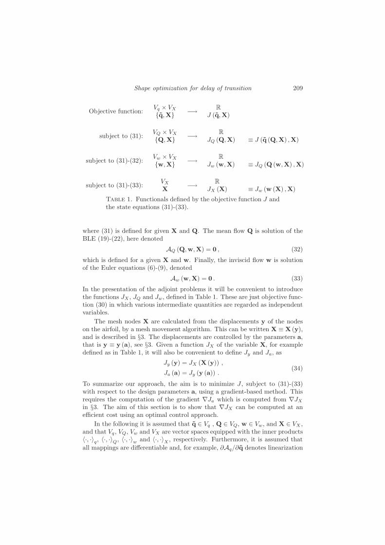
Shape optimization for delay of transition 209
Objective function: Vq ( VX
{q,X} #% RJ (q,X)
subject to (31): VQ ( VX
{Q,X} #% RJQ (Q,X) 1 J (q (Q,X) ,X)
subject to (31)-(32): Vw ( VX
{w,X} #% RJw (w,X) 1 JQ (Q (w,X) ,X)
subject to (31)-(33): VX
X #% RJX (X) 1 Jw (w (X) ,X)
Table 1. Functionals defined by the objective function J andthe state equations (31)-(33).
where (31) is defined for given X and Q. The mean flow Q is solution of theBLE (19)-(22), here denoted
AQ (Q,w,X) = 0 , (32)
which is defined for a given X and w. Finally, the inviscid flow w is solutionof the Euler equations (6)-(9), denoted
Aw (w,X) = 0 . (33)
In the presentation of the adjoint problems it will be convenient to introducethe functions JX , JQ and Jw, defined in Table 1. These are just objective func-tion (30) in which various intermediate quantities are regarded as independentvariables.
The mesh nodes X are calculated from the displacements y of the nodeson the airfoil, by a mesh movement algorithm. This can be written X 1 X (y),and is described in §3. The displacements are controlled by the parameters a,that is y 1 y (a), see §3. Given a function JX of the variable X, for exampledefined as in Table 1, it will also be convenient to define Jy and Ja, as
Jy (y) = JX (X (y)) ,
Ja (a) = Jy (y (a)) .(34)
To summarize our approach, the aim is to minimize J , subject to (31)-(33)with respect to the design parameters a, using a gradient-based method. Thisrequires the computation of the gradient "Ja which is computed from "JX
in §3. The aim of this section is to show that "JX can be computed at ane"cient cost using an optimal control approach.
In the following it is assumed that q ' Vq , Q ' VQ, w ' Vw, and X ' VX ,and that Vq , VQ, Vw and VX are vector spaces equipped with the inner products-·, ·.q, -·, ·.Q, -·, ·.w and -·, ·.X , respectively. Furthermore, it is assumed thatall mappings are di!erentiable and, for example, !Aq/!q denotes linearization
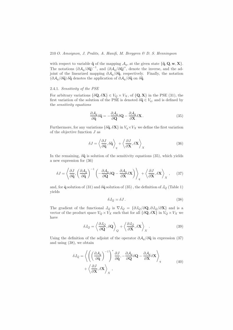
210 O. Amoignon, J. Pralits, A. Hanifi, M. Berggren & D. S. Henningson
with respect to variable q of the mapping Aq, at the given state {q,Q,w,X}.The notations (!Aq/!q)"1, and (!Aq/!q)$, denote the inverse, and the ad-joint of the linearized mapping !Aq/!q, respectively. Finally, the notation(!Aq/!q) 0q denotes the application of !Aq/!q on 0q.
2.4.1. Sensitivity of the PSE
For arbitrary variations {0Q, 0X} ' VQ ( VX , of {Q,X} in the PSE (31), thefirst variation of the solution of the PSE is denoted 0q ' Vq, and is defined bythe sensitivity equations
!Aq
!q0q = #!Aq
!Q0Q# !Aq
!X0X . (35)
Furthermore, for any variations {0q, 0X} in Vq(VX we define the first variationof the objective function J as
0J =M!J
!q, 0qN
q
+M!J
!X, 0X
N
X
(36)
In the remaining, 0q is solution of the sensitivity equations (35), which yieldsa new expression for (36)
0J =
O!J
!q,
-!Aq
!q
."1-#!Aq
!Q0Q# !Aq
!X0X.P
q
+M!J
!X, 0X
N
X
, (37)
and, for q solution of (31) and 0q solution of (35) , the definition of JQ (Table 1)yields
0JQ = 0J . (38)
The gradient of the functional JQ is "JQ = {!JQ/!Q, !JQ/!X} and is avector of the product space VQ(VX such that for all {0Q, 0X} in VQ(VX wehave
0JQ =M!JQ
!Q, 0Q
N
Q
+M!JQ
!X, 0X
N
X
. (39)
Using the definition of the adjoint of the operator !Aq/!q in expression (37)and using (38), we obtain
0JQ =
O+-!Aq
!q
."1,$
!J
!q,#!Aq
!Q0Q# !Aq
!X0X
P
q
+M!J
!X, 0X
N
X
,
(40)

Shape optimization for delay of transition 211
which is in turn rewritten using the definition of the adjoint of !Aq/!Q, and!Aq/!X, respectively, as
0JQ = #O-
!Aq
!Q
.$+-
!Aq
!q
."1,$
!J
!q, 0Q
P
Q
#O-
!Aq
!X
.$+-
!Aq
!q
."1,$
!J
!q, 0X
P
X
+M!J
!X, 0X
N
X
.
(41)
Therefore, by introducing the adjoint state q$, solution of the system-!Aq
!q
.$q$ =
!J
!q, (42)
we obtain that
!JQ
!Q= #
-!Aq
!Q
.$q$ and
!JQ
!X=!J
!X#-!Aq
!X
.$q$ . (43)
The cost for obtaining gradient of JQ is reduced to one solution of the system(42) and two matrix–vector products as shown in (43).
2.4.2. Sensitivity of the BLE
For arbitrary variations {0w, 0X} ' Vw ( VX , of {w,X} in the BLE (32), thefirst variation of the solution of the BLE is denoted 0Q ' VQ, and is definedby the sensitivity equations
!AQ
!Q0Q = #!AQ
!w0w # !AQ
!X0X . (44)
Furthermore, from the definition (39) and the expression of the gradient (43),for arbitrary variations {0Q, 0X} in VQ ( VX , the variation 0JQ is
0JQ =M#-!Aq
!Q
.$q$, 0Q
N
Q
+M!J
!X#-!Aq
!X
.$q$, 0X
N
X
. (45)
In the following, 0Q is solution of the sensitivity equation (44). The variation0JQ is expressed, making use of (45) and (44), as
0JQ =
O#-!Aq
!Q
.$q$,
-!AQ
!Q
."1-#!AQ
!w0w # !AQ
!X0X.P
Q
+M!J
!X#-!Aq
!X
.$q$, 0X
N
X
,
(46)
and, for Q solution of (32) and 0Q solution of (44) , the definition of Jw
(Table 1) yields0Jw = 0JQ . (47)

212 O. Amoignon, J. Pralits, A. Hanifi, M. Berggren & D. S. Henningson
The gradient of Jw is the vector {!Jw/!w, !Jw/!X} in the product spaceVw ( VX such that for all {0w, 0X} in Vw ( VX we have
0Jw =M!Jw
!w, 0w
N
w
+M!Jw
!X, 0X
N
X
. (48)
Using the adjoint of the inverse linearized BLE operator (!AQ/!Q)"1 in (46),0Jw (47) is expressed as
0Jw =
O#+-
!AQ
!Q
."1,$-
!Aq
!Q
.$q$,#!AQ
!w0w# !AQ
!X0X
P
Q
+M!J
!X#-!Aq
!X
.$q$, 0X
N
X
.
(49)
Using the adjoints of !AQ/!w and !AQ/!X enables us to rewrite relation (49)as
0Jw =
O-!AQ
!w
.$+-
!AQ
!Q
."1,$-
!Aq
!Q
.$q$, 0w
P
w
+
O-!AQ
!X
.$+-
!AQ
!Q
."1,$-
!Aq
!Q
.$q$, 0X
P
X
+M!J
!X#-!Aq
!X
.$q$, 0X
N
X
.
(50)
It suggests, as previously, to define an adjoint state Q$ as-!AQ
!Q
.$Q$ =
-!Aq
!Q
.$q$ . (51)
Setting Q$ in (50) and identifying the new expression with (48) we obtain
!Jw
!w=-!AQ
!w
.$Q$ and
!Jw
!X=!J
!X#-!Aq
!X
.$q$ +
-!AQ
!X
.$Q$ . (52)
The use of adjoint equations limits cost for obtaining the gradient of Jw tosolving the systems (42) and (51), as well as four matrix–vector products: oneto ’assemble’ the right-hand side of the adjoint system (51) and three to obtainthe final expression (52).
2.4.3. Sensitivity of the Euler equations
For arbitrary variations 0X ' VX , of X in the Euler equation (33), the firstvariation of solution of the Euler equation is denoted 0w ' Vw, and is definedby the sensitivity equation
!Aw
!w0w = #!Aw
!X0X . (53)

Shape optimization for delay of transition 213
Furthermore, for arbitrary variations {0w, 0X} in Vw ( VX the first variationof the functional Jw is expressed, from the gradient (52)
0Jw =M-
!AQ
!w
.$Q$, 0w
N
w
+M!J
!X#-!Aq
!X
.$q$ +
-!AQ
!X
.$Q$, 0X
N
X
(54)
In the following, 0w is the solution of the sensitivity equation (53), whichenables us to rewrite expression (54) as
0Jw =
O-!AQ
!w
.$Q$,#
-!Aw
!w
."1 !Aw
!X0X
P
w
+M!J
!X#-!Aq
!X
.$q$ +
-!AQ
!X
.$Q$, 0X
N
X
,
(55)
and, for w solution of (33) and 0w solution of (53), the definition of JX (Ta-ble 1) yields
0JX = 0Jw . (56)The gradient of JX is the vector "JX in the space VX such that for all 0X inVX we have
0JX = -"JX , 0X.X . (57)The adjoint of the linearized Euler operator is used in (55) to express 0JX (56)as
0JX =
O+-!Aw
!w
."1,$-
!AQ
!w
.$Q$,#!Aw
!X0X
P
w
+M!J
!X#-!Aq
!X
.$q$ +
-!AQ
!X
.$Q$, 0X
N
X
.
(58)
The adjoint instead of the linear operator !Aw/!X is used in (58) and leadsto
0JX =M!J
!X#-!Aq
!X
.$q$ +
-!AQ
!X
.$Q$, 0X
N
X
#O-
!Aw
!X
.$+-
!Aw
!w
."1,$-
!AQ
!w
.$Q$, 0X
P
X
,
(59)
The method of adjoint is again applied as we define an adjoint state w$, heresolution of the system
-!Aw
!w
.$w$ =
-!AQ
!w
.$Q$ , (60)
which enables us to give expression for the gradient (57)
"JX =!J
!X#-!Aq
!X
.$q$ +
-!AQ
!X
.$Q$ #
-!Aw
!X
.$w$ . (61)

214 O. Amoignon, J. Pralits, A. Hanifi, M. Berggren & D. S. Henningson
The total cost of this gradient evaluation is three adjoint systems (42),(51) and (60), and five matrix–vector products: two for the assembly of theright-hand-sides of the systems (51) and (60), and three for the final expression(61).
2.5. Adjoint equations
The concise description given in §2.4 gives an expression of the gradient "JX
(61), which is a function of three adjoint states q$, Q$ and w$. These statesare the solutions of the adjoint of the parabolized stability equations (42), ad-joint of the boundary layer equations (51) and adjoint of the Euler equations(60), respectively. There are in principle two di!erent approaches on how toderive these adjoint equations. In the first, sometimes denoted the “discreteapproach” or “discretize-then-di!erentiate”, the adjoint equations are derivedfrom the discretized set of state equations. In the second approach, sometimesdenoted the “continuous approach” or “di!erentiate-then-discretize”, the ad-joint equations are derived from the continuous state equations. The continuousadjoint equations are then discretized, commonly in a similar way as the cor-responding state equations, in which the original code written for solving thestate is reused with some modifications.
2.5.1. Adjoint of the Parabolized Stability Equations
The adjoint of the parabolized stability equations (42) are derived using acontinuous approach. The complete derivation is found in Pralits et al. (2000)and they are here given as
Aq$ + B!q$
!x3+ C !2q$
(!x3)2+ D 1
h1
!q$
!x1= S$
P, (62)
!
!x1
* +#
0q$H
-!A!(
+!B!(
.q h1dx3 =
@A
B
0 0x1 /' [Xms, Xme],
#i|$|2* +#
0qHM q h1dx3 0x1 ' [Xms, Xme],
(63)
where
S$P =
@EA
EB
#r$!q!x1# !(r$q)
!x10x1 /' [Xms, Xme],
#r$!q!x1# !(r$q)
!x1+ ,MHq|$|2 0x1 ' [Xms, Xme],

Shape optimization for delay of transition 215
and
A = AH # !BH
!x3# m13 BH +
!2CH
(!x3)2+ 2 m13
!CH
!x3# !DH
!x1,
B = #BH + 2!CH
!x3+ 2 m13 CH,
C = CH,
D = #DH.
Here, q$ = ("$, u$, v$, w$, '$)T, and the above equations are subject to thefollowing boundary conditions
[u$, v$, w$, '$] (x1, 0) = [0, 0, 0, 0] 0x1 ' [X0, X1],lim
x3%+#[u$, v$, w$, '$] (x1, x3) = [0, 0, 0, 0] 0x1 ' [X0, X1].
The initial conditions are
q$(X1, x3) = (1 # ,)q$
1(x3) 0x3 ' [0, +&),r$(X1) = (1 # ,)r$1 0x3 ' [0, +&),
with q$1 and r$1 evaluated at x1 = X1 as
q$1 = |$|2D+(M # c1I)q, r$1 = |$|2 c1,
c1 =
* #
0(h1qHM D+H
-!A!(
+!B!(
.q# iqHM q) dx3
* #
0qHD+H
-!A!(
+!B!(
.q h1 dx3
,(64)
where D+ = (DH)"1. Equation (62) is solved by backward integration in space.Even though it is a linear equation, in order to reuse the code developed tosolve the PSE iteratively to satisfy the auxiliary condition, at each streamwiseposition r$ is solved iteratively such that expression (63) is satisfied. The righthand side of equation (62) and the initial condition depend on the choice ofobjective function, i. e. the value of ,.
2.5.2. Adjoint of the Boundary Layer Equations
The adjoint of the boundary-layer equations are derived using a continuousapproach. Details regarding the derivation is found in Pralits (2001) and Pralits

216 O. Amoignon, J. Pralits, A. Hanifi, M. Berggren & D. S. Henningson
& Hanifi (2003) and they are here given as
"!(h1W
$)!x3
# h1"
-!U
!x3U$ +
!V
!x3V $ + cp
!T
!x3T $.
= S$W , (65)
!("UU$)!x1
+!(h1"WU$)
!x3# "
-!U
!x1U$ +
!V
!x1V $ # !W $
!x1+ cp
!T
!x1T $.
+
(% # 1)M2 dPe
dx1T $ # 2(% # 1)
ReM2 !
!x3
-h1µ
!U
!x3T $.
+
1Re
!
!x3
-µ!(h1U
$)!x3
.= S$
U , (66)
!("UV $)!x1
+!(h1"WV $)
!x3# 2(% # 1)
ReM2 !
!x3
-h1µ
!V
!x3T $.
+
1Re
!
!x3
-µ!(h1V
$)!x3
.= S$
V , (67)
cp!("UT $)!x1
+ cp!(h1"WT $)
!x3+"U
T
-!U
!x1U$ +
!V
!x1V $ # !W $
!x1
.+
"U
Tcp!T
!x1T $ +
$
RePr!2(h1T
$)(!x3)2
(% # 1)Re
M2 dµ
dT
C-!U
!x3
.2
+-!V
!x3
.2D
T $ #
1Re
dµ
dT
/!U
!x3
!(h1U$)
!x3+!V
!x3
!(h1V$)
!x3
0= S$
E , (68)
where the right hand side S$B = (S$
W , S$U , S$
V , S$E)T is given as
S$B =
2(FW , FU , FV , FT + FW W/T )T h1 0x1 ' (X0, X1),
0 0x1 ' (XS , X0],(69)
The non-zero right hand side is the coupling between the APSE and the ABLEand express the sensitivity of the PSE with respect the variations in W , U ,V and T respectively. A detailed description is found in Pralits (2001). Theabove equations are subjected to the following boundary conditions
/U$, V $,
!(h1T$)
!x3
0(x1, 0) = [0, 0, 0] 0x1 ' [X0, X1],
limx3%+#
[U$, V $, W $, T $] (x1, x3) = [0, 0, 0, 0] 0x1 ' [X0, X1].
The initial condition at x1 = X1 is given as
Q$(X1, x3) = 0. 0x3 ' [0, +&),

Shape optimization for delay of transition 217
These equations are linear oppose to the BLE but are however solved in asimilar iterative way as was outlined in §2.2.1 in order to reuse the existingsolver for the boundary layer equations. The ABLE are solved by backwardintegration in the streamwise direction. At each streamwise position we obtainthe solution of Q$ = (U$, V,$ T $) from equations (66)–(68) using the boundaryconditions above for a given value of W $. Equation (65) is integrated in thewall-normal direction in order to obtain W $. The solution at each streamwiseposition is considered converged when the relative variation of W $ is below aspecified value.
The coupling between the Euler and the boundary-layer equations is thepressure distribution Pe and the mesh given by the nodal coordinates X. Avariation of the geometry which a!ects the Euler solution, will therefore ap-pear as variations of the pressure distribution in the boundary layer equations,which consequently will a!ect the solution of the stability equations. In Pralitset al. (2002), the possibility of an optimal control problem using the pressuredistribution as control variables and the total disturbance kinetic energy as theobjective function, was considered. From the coupled APSE and ABLE for in-compressible flows, an expression was derived for the gradient of the objectivefunction with respect to the pressure distribution. From the present APSE andABLE a similar expression can be evaluated and is here given as
"JP =* +#
0
-#!U$
!x1+ (% # 1)M2!(T $U)
!x1
.dx3 0x1 ' (XS , X1). (70)
Setting the Mach number equal to zero in expression (70), we find exactly thesame expression as the one derived in Pralits et al. (2002). Note that a variationof X will also a!ect the nodal coordinates of the BLE and PSE. This can beseen in expression (61).
2.5.3. Adjoint of the Euler equations
The adjoint equations (60) are solved following the same technique used forsolving the Euler equations (§2.1), by explicit time integration of the system
Vidw$
i
dt+ R$
i = 0, 0i ' V(&) (71)
until the residuals R$i vanish within some tolerance. Derivation of the adjoint
of the Euler equations can be found in Amoignon (2003). The following givesexpression for the adjoint residuals

218 O. Amoignon, J. Pralits, A. Hanifi, M. Berggren & D. S. Henningson
R$i =
%
j&Ni
/!(fi · nij)!wi
0T3w$
i #w$j
4
2+%
j&Ni
d$ij 0i ' V(&) ,
R$i =
%
j&Ni
/!(fi · nij)!wi
0T3w$
i #w$j
4
2
+%
j&Ni
d$ij +
%
j&Ni
/!(fbc
i · ni)!wi
0T
w$i 0i ' V(!&) ,
R$i =
%
j&Ni
/!(fi · nij)!wi
0T3w$
i #w$j
4
2
+%
j&Ni
d$ij +
%
j&Ni
/!(fbc
i · ni)!wi
0T
w$i # g$
i 0i ' V(!&o) ,
(72)
where V(!&o) is the set of nodes at which the pressure Pe is measured, accord-ing to the definition of the BLE (19)–(22). The right-hand-side of equation (60),is included in the residuals
g$i =
--!AQ
!w
.$Q$.
i
(73)
The adjoint d$ of the artificial dissipation fluxes d (15) are obtained by freezingthe artificial viscosities (see Amoignon 2003), that is, the di!erentiation of .ij2and .i4 with respect to wh is assumed to give terms which can be neglected.This assumption yields that
d$ij = .ij2 (w$
i #w$j ) + (.i"2w$
i # .j"2w$j ) . (74)
However, the resulting truncation error may not be negligible in the computa-tion of the gradient "J . This is studied later in this report through numericaltests. A similar freezing of the coe"cients in the farfield boundary conditionsyields the following expression for the Jacobian of the farfield flux:
!(fbci · ni)!wi
=! (f · ni)!vi
L (ni,v#)H (#i)L"1 (ni,v#)dvi
dwi. (75)
The Jacobian of the Euler wall flux function is expressed as follows
!3fbci · ni
4
!wi= (% # 1)
I
J12 |ui|2#ui
1
K
L . (76)
3. Implementation issues3.1. Mesh displacements
In the current study an explicit a"ne mapping is used to smoothly propagatechanges in the geometry to the entire mesh. It is formulated as
Xk = X0 + Lyk . (77)

Shape optimization for delay of transition 219
where yk ' Rn is the vector of node displacements on the airfoil, for the designnumber k, Xk ' R2N is the vector of all nodal coordinates (N is the totalnumber of nodes in the grid), L ' R2N'n is a constant coe"cients matrix, and,X0 is the reference mesh, defined by its vector of nodal coordinates. Given thegradient "JX , of a functional JX such as defined in Table 1, the gradient ofthe functional Jy (y) 1 JX (X (y)) is obtained by a matrix–vector product
"Jy = LT"JX . (78)
The definition of L was possible because the meshes we used here are issuedfrom structured grids. More general schemes are needed when using generalunstructured meshes (see Berggren 2003).
3.2. Parameterization of displacements and constraints
In shape optimization, the combination of gradient-methods and piecewisepolynomial interpolations, such as B-splines, may induce oscillations in theshapes, as investigated in Frank & Shubin (1992). In the current approach,smooth shapes are obtained, together with geometric constraints, by takingthe vectors of displacements y that are solution of a minimization problem (seeAmoignon 2003) of the form
y =
2minv&Rn
12vT Asv # vT Msa ,
CTy = b, (79)
where As is the sti!ness matrix associated with the Laplace operator, Ms is amass matrix, C is a matrix whose rows are the gradients of constraints imposedon the displacements (in Rn'm) and b is the vector of values imposed to theconstraints (in Rm). The solution y to the above system is the vector ofdisplacements, which, according to the norm defined by the sti!ness matrixAs, is the closest to the solution of the discretized Laplace equation defined by
Asy = Msa , (80)
and that fulfills exactly the constraints
CTy = b . (81)
Such a parameterization implies that the controls are the vector a, right sideof the Laplace equation (80), and the vector b, right side of the constraintsrelations (81). Therefore, from the gradient with respect to the displacements"Jy, that is eventually obtained by (78) it is needed to calculate a gradient withrespect to {a,b}, the control variables in our method. This can be achievedby solving an adjoint problem of the form (see Amoignon 2003)
-AT
s #C#CT 0
.-y$
#$
.=-"Jy
0
., (82)
from which it holds that
"Ja = MTs y$ and "Jb = ##$ . (83)

220 O. Amoignon, J. Pralits, A. Hanifi, M. Berggren & D. S. Henningson
3.3. Optimization algorithm
All numerical tests carried out here are formulated so that aerodynamic con-straints (lift and pitch) are integrated to the objective function via a simplepenalization technique. Geometrical constraints (volume and fixed domain)can be treated as simple bounds constraints via the parameterization previ-ously discussed (see §3.2). However, the geometrical constraints are equalityconstraints, so that the the right hand side, b in (79), will be a constant vector.The only control parameter used in our applications is therefore the vector a,expression (79).
The optimization algorithm is the limited memory quasi-Newton methoddeveloped by Byrd et al. (1995). It is based on a limited memory BFGS approx-imation of the Hessian matrix of the functional f , and a gradient projectionmethod is used to account for bounds on the data which makes it suitable forlarge scale problems where only the gradient of f is available.
3.4. Solution procedure
A simple chart of the order in which the state and adjoint equations are solvedand gradients are evaluated in order to perform optimal NLF is given in figure 2.There, k denotes the iteration number and the procedure is as follows:
1. For k = 1, we start with an initial Euler mesh X0
2. The Euler, BLE and PSE are solved in the given order3. The objective function Jk is evaluated4. The adjoint equations, APSE, ABLE and AEuler are solved5. The gradients "Jk
X , "Jky and "Jk
a are evaluated in the given order6. A new control parameter ak+1 is calculated2 using the gradient "Jk
a
7. If k > 1, check convergence: If |(Jk+1 # Jk)/Jk| < ., else3 continue8. A new mesh Xk+1 is calculated from the new control parameter ak+1
9. Goto 2.
4. Numerical testsThe accuracy of the gradient "Ja (83) of the objective function is a criticalissue in optimization. The first order necessary optimality condition is that thegradient of the objective function or, of the Lagrangian, is zero at an optimaldesign. Di"culties related to low accuracy, such as di"culty to find descentdirections even far from the optimal design, are quite common. There are twopossible causes of inaccuracies in our calculation of the gradient. As mentionedpreviously, the derivation of the adjoint of the discretized Euler equations makesuse of an approximation as it does not linearize the coe"cients of the 2nd or-der artificial dissipation. E!ects of this approximation are investigated in §4.1.The adjoint equations of the BLE and PSE are derived from the continuous
2In the computations shown here, the L-BFGS-B routine was used, normally requiring severalfunctional and gradient evaluations in order to build up the approximative Hessian matrix.3Several convergence criteria exist in the L-BFGS-B routine, (see Zhu et al. 1994)

Shape optimization for delay of transition 221
2Euler BLE PSE
APSEABLEAEuler
ak+1% yk+1% Xk+1
"Jka 3 "Jk
y 3 "JkX
Figure 2. Flow chart for the case of minimizing the distur-bance kinetic energy using the parameter a to control theshape of geometry.
state equations. The e!ects of this method on the accuracy of the gradients ofthe type "Jw (for JX defined as in Table 1) is investigated in §4.2.1. The cal-culation of "Ja is obtained by coupling the three systems of adjoint equations,and the accuracy is investigated in §4.2.2.
The accuracy of the gradient at a design point a can be analyzed, compar-ing the value obtained from the solution of the adjoint equations, with the oneestimated by finite di!erences as
("Ja)k *Ja(a + .aek)# Ja(a# .aek)
2.a, (84)
where ek is the vector having component k equal to 1 and all other componentsbeing 0. Several calculations of ("Ja)k is commonly performed, using di!erentvalues of .a in order to find the best compromise between accuracy and roundingerrors, the last being inherent to the finite di!erence method. The relativeerror between the gradient obtained by adjoint method "ADJa and the oneapproximated by finite-di!erences "Ja can be calculated as
err)Ja =,"ADJa #"Ja,
,"Ja,, (85)
where ,., denotes the norm in Rn defined by the dot product.These tests are performed on di!erent C-type meshes of the RAE 2822.
They are here denoted coarse, medium and fine, and the sizes are:
• Coarse: 3412 nodes with 112 nodes on the airfoil.• Medium: 13352 nodes with 224 nodes on the airfoil.• Fine: 52816 nodes with 448 nodes on the airfoil.
4.1. The inviscid case
Possible inaccuracies, due to the approximation made in the Euler adjointequations, are expected to be independent from the forcing of the these equa-tions. In our investigation the right-hand-side of the adjoint equation (60) is
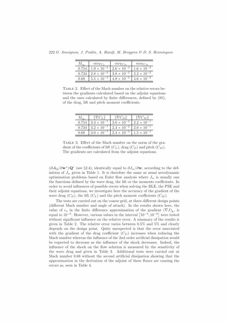
222 O. Amoignon, J. Pralits, A. Hanifi, M. Berggren & D. S. Henningson
M# err)CL err)CD err)CM
0.754 1.9( 10"2 2.6( 10"2 1.6( 10"2
0.734 2.8( 10"2 3.8( 10"2 2.2( 10"2
0.68 5.5( 10"3 4.9( 10"2 4.6( 10"3
Table 2. E!ect of the Mach number on the relative errors be-tween the gradients calculated based on the adjoint equationsand the ones calculated by finite di!erences, defined by (85),of the drag, lift and pitch moment coe"cients.
M# ,"CL, ,"CD, ,"CM,0.754 3.3( 10"1 3.0( 10"2 2.2( 10"1
0.734 3.2( 10"1 2.3( 10"2 2.0( 10"1
0.68 3.0( 10"1 2.4( 10"3 1.5( 10"1
Table 3. E!ect of the Mach number on the norm of the gra-dient of the coe"cients of lift (CL), drag (CD) and pitch (CM ).The gradients are calculated from the adjoint equations.
(!AQ/!w$)Q$ (see §2.4), identically equal to !Jw/!w, according to the def-inition of Jw given in Table 1. It is therefore the same as usual aerodynamicoptimization problems based on Euler flow analysis where Jw is usually onethe functions defined by the wave drag, the lift or the moments coe"cients. Inorder to avoid influences of possible errors when solving the BLE, the PSE andtheir adjoint equations, we investigate here the accuracy of the gradient of thewave drag (CD), the lift (CL) and the pitch moment coe"cients (CM ).
The tests are carried out on the coarse grid, at three di!erent design points(di!erent Mach number and angle of attack). In the results shown here, thevalue of .a in the finite di!erence approximation of the gradient ("J)k, isequal to 10"6. However, various values in the interval
810"4, 10"8
9were tested
without significant influence on the relative error. A summary of the results isgiven in Table 2. The relative error varies between 0.5% and 5% and clearlydepends on the design point. Quite unexpected is that the error associatedwith the gradient of the drag coe"cient (CD) increases when reducing theMach number whereas the influence of the 2nd order artificial dissipation wouldbe expected to decrease as the influence of the shock decreases. Indeed, theinfluence of the shock on the flow solution is measured by the sensitivity ofthe wave drag and given in Table 3. Additional tests were carried out atMach number 0.68 without the second artificial dissipation showing that theapproximation in the derivation of the adjoint of these fluxes are causing theerrors as, seen in Table 4.
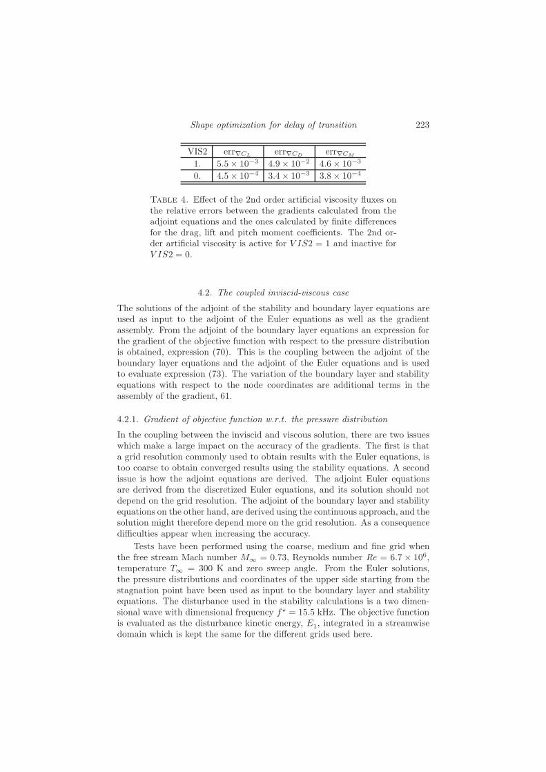
Shape optimization for delay of transition 223
VIS2 err)CL err)CD err)CM
1. 5.5( 10"3 4.9( 10"2 4.6( 10"3
0. 4.5( 10"4 3.4( 10"3 3.8( 10"4
Table 4. E!ect of the 2nd order artificial viscosity fluxes onthe relative errors between the gradients calculated from theadjoint equations and the ones calculated by finite di!erencesfor the drag, lift and pitch moment coe"cients. The 2nd or-der artificial viscosity is active for V IS2 = 1 and inactive forV IS2 = 0.
4.2. The coupled inviscid-viscous case
The solutions of the adjoint of the stability and boundary layer equations areused as input to the adjoint of the Euler equations as well as the gradientassembly. From the adjoint of the boundary layer equations an expression forthe gradient of the objective function with respect to the pressure distributionis obtained, expression (70). This is the coupling between the adjoint of theboundary layer equations and the adjoint of the Euler equations and is usedto evaluate expression (73). The variation of the boundary layer and stabilityequations with respect to the node coordinates are additional terms in theassembly of the gradient, 61.
4.2.1. Gradient of objective function w.r.t. the pressure distribution
In the coupling between the inviscid and viscous solution, there are two issueswhich make a large impact on the accuracy of the gradients. The first is thata grid resolution commonly used to obtain results with the Euler equations, istoo coarse to obtain converged results using the stability equations. A secondissue is how the adjoint equations are derived. The adjoint Euler equationsare derived from the discretized Euler equations, and its solution should notdepend on the grid resolution. The adjoint of the boundary layer and stabilityequations on the other hand, are derived using the continuous approach, and thesolution might therefore depend more on the grid resolution. As a consequencedi"culties appear when increasing the accuracy.
Tests have been performed using the coarse, medium and fine grid whenthe free stream Mach number M# = 0.73, Reynolds number Re = 6.7 ( 106,temperature T# = 300 K and zero sweep angle. From the Euler solutions,the pressure distributions and coordinates of the upper side starting from thestagnation point have been used as input to the boundary layer and stabilityequations. The disturbance used in the stability calculations is a two dimen-sional wave with dimensional frequency f! = 15.5 kHz. The objective functionis evaluated as the disturbance kinetic energy, E1, integrated in a streamwisedomain which is kept the same for the di!erent grids used here.

224 O. Amoignon, J. Pralits, A. Hanifi, M. Berggren & D. S. Henningson
50 55 60 65 70 75−5
−2.5
0
2.5
5x 10⁻⁵
dJ/d
P
k (index of control parameter)
(a)
100 110 120 130 140 150−5
−2.5
0
2.5
5x 10⁻⁵
dJ/d
P
k (index of control parameter)
(b)
200 220 240 260 280 300−5
−2.5
0
2.5
5x 10⁻⁵
dJ/d
P
k (index of control parameter)
(c)
Figure 3. Gradient of objective function with respect to pres-sure distribution. Comparison between finite-di!erence ap-proximation (solid-stars) and adjoint solution (solid-plus) com-puted on (a) coarse, (b) medium, and (c) fine grid.
In figure 3 results are shown for a comparison between expression (70) anda finite di!erence approximation of the gradient of the objective function withrespect to the pressure distribution. The latter is evaluated in the same wayas expression (84), where the design a has been replaced by the pressure P .Computations have been performed for di!erent values of the finite-di!erencestep .p, and these values are 10"4, 10"5, 10"6, 10"7. Only the results for.p = 10"5 are shown. A first thing to note is that the gradient evaluated usingthe finite-di!erence approximation appears to converge as the grid resolutionincreases. This is due both to the solution of the pressure distribution con-verging in the Euler computation, and the solution of the stability equationsconverging as the grid is refined. Secondly it can be seen that the di!erence

Shape optimization for delay of transition 225
50 100 150 200 250 300400
600
800
1000
1200
1400
Re
k (index of control parameter)
(a) (b) (c)
Figure 4. Local Reynolds number as a function of the controlparameter k (a) coarse grid, (b), medium grid, (c) fine grid.
between gradients obtained from the finite-di!erence approximation and thoseobtained from the solution of the adjoint equations, decreases as the grid isrefined. This is due to the continuous approach used to derive the adjointequations.
The adjoint of the boundary layer and stability equations used here havebeen used in other problems concerning gradient evaluations for the purpose ofoptimal control problems (see Pralits et al. 2000; Pralits & Hanifi 2003; Pralitset al. 2002). There, di!erent grid resolutions expressed as a step length inthe local Reynolds number %Re, where Re =
$Uex/&e, were tested to see the
e!ect on the gradient accuracy. In Pralits et al. (2000), it was shown that a steplength of %Re = 20 was needed to converge the physical result for a flat plateboundary layer with zero pressure gradient. Further, it was shown that a valueof %Re = 10 was needed to obtain a relative di!erence of 10"3 between theapproximative finite di!erence calculation and the adjoint calculation, in themajor part of the computational domain. In figure 4, the step length expressedas local Reynolds number has been plotted for the di!erent grids used here.It can be seen that the step length is almost constant through out respectivedomain and the values are %Re = 50, 25 and 13 for the coarse, medium and finegrids, respectively. Due to the variation of the pressure gradient along wingprofiles, the step lengths found in the previous study of flat-plate boundarylayers, might not be small enough to obtain the same convergence in the resultsand accuracy of the gradients in the case studied here. It should further benoted that the finest grid shown in figures 3 and 4, is computationally heavy forthe Euler solver, and might not be reasonable to use in the case of optimization.
One option to increase the accuracy of the gradients is to use some in-terpolation technique for the calculation of the boundary layer, stability and

226 O. Amoignon, J. Pralits, A. Hanifi, M. Berggren & D. S. Henningson
0 0.01 0.02 0.03 0.04 0.050
0.4
0.8
1.2
1.6
Ue
s/c
00
0.05
0.1
0.15
0 0.002 0.0040
0.05
0.1
0.15
(a)
0 0.005 0.01 0.015 0.020
50
100
150
dUe/d
xs/c
(b)
Figure 5. Comparison of Ue and !Ue/!x1 between originalmedium grid (solid), and interpolated values using quadraticpolynomial on half grid (dot), cubic splines on half grid (dash),and cubic splines on whole grid (dash-dot). The refined gridsare obtained by inserting one additional point in between oldgrid points.
corresponding adjoint equations, given the solution of the pressure distributioncomputed on a ’coarse’ grid. Such an approach could also be favorable whenthree-dimensional flows are considered, and thus the computational e!ort in-crease considerably for the Euler equations. The outline of an interpolationapproach can be made as follows: the pressure distribution from the Eulersolution is interpolated on a grid with higher resolution, the boundary layer,stability and corresponding adjoint equations are solved on the new grid, thegradient "JP is evaluated and then interpolated back on the original grid.Here, decisions need to be made on how to produce the new grid distribution,i. e. the distribution of the coordinate x/c describing the geometry, and fur-ther which interpolation scheme to use, in order to obtain y/c and Pe. Oneapproach to refine the grid is to insert additional node points in between theold ones. An advantage of inserting additional nodes in between the old ones,is that the function values of the original nodes can be used in the chosen in-terpolation scheme. Here, we have chosen to interpolate Ue instead of Pe. Infigure 5, results of Ue and !Ue/!x1 can be seen using di!erent interpolationschemes. We have used the medium grid shown earlier and the new grid isobtained by inserting an additional point in between the old grid points, i. e.the new grid has twice as many points as the original one. Two calculationshave been performed when interpolation has been made using only the upperpart of the wing, i. e. from the stagnation point to the trailing edge. Theinterpolation schemes are a piecewise quadratic polynomial and cubic splines.In addition a cubic spline interpolation has been made when the whole gridwas used. In figure 5a, results are shown of Ue close to the leading edge. A

Shape optimization for delay of transition 227
120 125 130 135 140−1
−0.5
0
0.5
1x 10⁻⁵
dJ/d
P
k (index of control parameter)
Figure 6. Comparison of the gradient !J/!Pe computedfrom the solution of the adjoint equations using the mean flowscorresponding to the cases in figure 5. A comparison is madewith the finite di!erence approximation of the gradient (solid-circle).
close up around the leading edge show that the magnitude of Ue of both caseswhere only the upper part of the wing was used in the interpolation, is largerat the first interpolation point. The streamwise derivative of the free streamvelocity corresponding to the cases in figure 5a are shown in figure 5b. Therespective interpolated mean flows were then used to compute gradient "JPby solving the PSE, APSE and ABLE. In figure 6 a comparison is made be-tween gradient computed using the finite di!erence approximation, and thoseobtained using the adjoint solutions. The gradient computed by solving theadjoint equations on the original grid is included for comparison. There, itis seen that the gradient computed using the piecewise quadratic polynomialinterpolation technique oscillates and deviates most from the finite di!erenceapproximation. The cases of using the cubic splines cannot be distinguishedfrom one another, and in comparison with the gradient computed on the orig-inal grid using the adjoint equations, a small improvement has been obtained.In the results of shape optimization for transition delay shown in this report,no interpolation technique has been used.
4.2.2. Gradient of objective function w.r.t. the shape parameterization
In the previous sections, tests have been performed to assess the accuracies ofthe inviscid (§4.1), and viscous parts (§4.2.1) separately. In this section, weinvestigate the accuracy of the gradient "Ja (83) which will be used in the op-timization procedure, when the objective function is based on a measure of thedisturbance kinetic energy. The reference case, denoted FD, is computed using

228 O. Amoignon, J. Pralits, A. Hanifi, M. Berggren & D. S. Henningson
0 30 60 90 120 150 180 210 240−6
−4
−2
0
2
4
6
8
Gra
d J k
k (index of control parameter)
Gradients
Figure 7. M# = 0.734 - Gradients of the objective function(Disturbance kinetic energy) with respect to the optimizationparameters (parameters that control the shape of the airfoil).The curves show FD (solid), ADJ1 (dot), ADJ2 (dash). Theerror between the FD and respective adjoint solution are: FD–ADJ1 (17.2%), FD–ADJ2 (4.95%), and FD–ADJ3 (4.85%, notshown).
the finite di!erence approximation of the gradient given by expression (84),which is evaluated solving consecutively the Euler, BLE and PSE. The ob-jective function in all tests performed here is given as the disturbance kineticenergy of a single disturbance integrated in a defined streamwise region, ex-pression (29) with K=1. The gradient "Ja is calculated from the gradient"JX (61) by variables transformations, from the nodal coordinates X to thedisplacements of the shape y, according to (78), and, from the displacementsof the shape y to the right side of the Laplace equation a, which requires tosolve (82) and to apply (83). The gradient "JX is given by expression (61)
"JX =!Jq
!X#-!Aq
!X
.$q$ +
-!AQ
!X
.$Q$
Q RS Tcont.
#-!Aw
!X
.$w$ .
Q RS Tdiscr.
As outlined in §3, it is evaluated from three systems of adjoint equations whichare solved in the following order
APSE % ABLEQ RS Tcont.
% adjoint Euler,Q RS Tdiscr.
where each calculation depends on the solution of the previous one. The APSEand ABLE are derived using the continuous approach, while the adjoint Euler

Shape optimization for delay of transition 229
0 30 60 90 120 150 180 210 240−10
−8
−6
−4
−2
0
2
4
6x 10⁻⁵
Gra
d J k
k (index of control parameter)
Gradients
Figure 8. M = 0.68 - Gradients of the objective function(Disturbance kinetic energy) with respect to the optimizationparameters (parameters that control the shape of the airfoil).The curves show FD (solid), ADJ2 (dash). The error is: FD–ADJ2 (0.02%)
is derived using the discrete approach. This is above denoted cont., and discr.,respectively. The latter has in the previous sections shown to be more accurateon the grids used here. In this section we therefore investigate the influence ofthe solution of the adjoint Euler, and the solution of the APSE and ABLE, onthe accuracy of the gradient which will be used in the optimization. This ismade by comparing the accuracy of the gradient computed from the solutionof all adjoint equations with the one evaluated from the solution of the adjointEuler in which the right hand side, see expression (60), is approximated by finitedi!erences. The right hand side is evaluated from expression (70) (!J/!P )when the solution of the APSE and ABLE are used. The finite di!erenceapproximation used here is the same that was used in §4.2.1. In addition, theinfluence of including the geometrical terms in the gradient evaluation from thesolution of the PSE, APSE and ABLE (denoted cont.) is investigated.
The di!erent cases are summarized below:
• FD: finite di!erence approximation of the gradient given by expres-sion (84), computed solving the Euler, BLE and PSE.
• ADJ1: gradient evaluated from the solution of the adjoint Euler, ABLE,and APSE
• ADJ2: gradient evaluated from the solution of the adjoint Euler. Theright hand side of the adjoint Euler, evaluated from !J/!P , is approxi-mated by finite di!erences computed by BLE and PSE.

230 O. Amoignon, J. Pralits, A. Hanifi, M. Berggren & D. S. Henningson
• ADJ3: gradient evaluated from the solution of the adjoint Euler, andby a finite di!erence approximation of the terms from the BLE andPSE. The right hand side of the adjoint Euler, evaluated from !J/!P ,is approximated by finite di!erences computed by BLE and PSE.
The relative di!erence between the FD and respective gradient evaluated fromthe solution of the adjoint equations, is calculated using expression (85). In thefirst test we consider the medium grid when the Mach number M# = 0.734. Apart of the geometry around the leading edge is kept fixed, and a comparison ismade between the FD and respective adjoint solution outlined in the summaryabove. The gradients are plotted as functions of the index of the surface nodes,where index 224 denote the trailing edge. The fixed region around the leadingedge is given between indexes 80 and 119. The largest error, 17.2%, is foundin the comparison between the FD and the complete adjoint solution, ADJ1.When the right hand side of the adjoint Euler equations is approximated byfinite di!erences, the error is reduced to 4.95%. Including the geometricalterms obtained from the BLE and PSE in the gradient evaluation (ADJ3) onlyreduces the error by 0.1% compared to the previous case (ADJ2).
The influence of including the second artificial viscosity on the gradientaccuracy was shown in (§4.1) for the inviscid flow equations. As the influenceis expected to decrease in the absence of a shock, a test was performed alsohere. We consider the flow at Mach number 0.68, and the surface is kept fixedeverywhere, except for the region where the objective function is evaluated. Infigure 8, a comparison is made between the FD and ADJ2. The error in thiscase is 0.02%.
5. Optimization results5.1. Description of the cases
Following the study performed on the accuracy of the sensitivities obtainedusing the continuous adjoint, §4.2, we chose to perform the optimization on themedium grid. Viscous calculations (RANS) are also carried out with EDGE4
by Eliasson (2001) prior to and after some of the optimization tests in orderto compare the N-factors based on the pressure distribution obtained fromthe viscous calculation with those that are computed using the Euler pressuredistribution. These calculations are also used to compare the viscous dragbetween the initial and the final optimized design. The C-type grid for RANScalculations has the size:
• Medium ’RANS’ mesh: 22088 nodes with 224 nodes on the airfoil.
In a first series of tests the objective is to reduce the disturbances kinetic energy.The only constraints are geometrical and imposed using the parameterizationgiven in §3.2. The objective function to minimize is the total disturbancekinetic energy of a single disturbance, E1 from expression (29). There are
4The turbulence model used is the EARSM by Wallin & Johansson (2000) and the k ! "model.

Shape optimization for delay of transition 231
several reasons for imposing geometrical constraints. A constant volume isintuitively a way to account for other industrial constraints such as having aminimum fuel tank capacity in the wings or a maximum weight of the materialstructure. The displacements of the nodes should not be allowed to be constantover all nodes, which would mean a translation of the wing. To remove thissingularity one point should remain fixed, and our choice is the trailing edge.In addition, we chose to fix a region of the airfoil around the leading edge inorder to prevent changes in the position of the stagnation point.
To summarize, the geometrical constraints are:
• Constant volume,• Constant position of the trailing edge,• Fixed region around the leading edge (between 0 of the chord length
and Xms given in Table 5).
In order to test if the optimization can account for the usual aerodynamicrequirements, two additional tests are carried out with a modified objectivefunction, denoted JC . The aim is to simultaneously reduce the disturbancekinetic energy and the wave drag, and in addition penalize changes in the coef-ficients of lift, and pitch-moment. The geometrical constraints are identical tothe first type of optimization which is described above. The modified objectivefunction is given as
JC = #UE1 + #DCD +12#L
3CL # C0
L
42 +12#M
3CM # C0
M
42, (86)
where E1 is the functional from expression (29), CD, CL and CM are the drag,lift, and pitch moment coe"cients, respectively
CD =%
i ' V(!&w)
pini · dD12"#v2
#Sref,
CL =%
i ' V(!&w)
pini · dL12"#v2
#Sref,
CM =%
i ' V(!&w)
pidM ·3xi #Oref.
4( ni
12"#v2
#SrefLref.
(87)
were dD is a unit vector in the direction of the farfield velocity, dD = #v#/|v2#|,
dL is a unit vector orthogonal to dD and, dM is a unit vector orthogonal todD and dL.
The values C0L and C0
M are the lift and pitch-moment coe"cients for theinitial design. In expression (86), we take the square of the deviation of lift andpitch with respect to the initial design in order to penalize both an increaseand decrease during the optimization. The real numbers {#U ,#D,#L,#M} are

232 O. Amoignon, J. Pralits, A. Hanifi, M. Berggren & D. S. Henningson
Case Objective M# Re# f$ [kHz] )$ 8m"19
Xms Xme
T11 E1 0.734 1.7 107 15.5 0 0.043 0.45T12 E1 0.734 6.5 106 11 500 0.043 0.45T21 E1 0.68 1.6 107 16.5 0 0.039 0.45T31 JC 0.734 1.7 107 15.5 0 0.043 0.45T32 JC 0.734 6.5 106 11 500 0.043 0.45
Table 5. Optimization tests description.
scaling factors calculated as
#U =1
10E01
, #D =1
10C0D
, #L =10
3C0
L
42 , #M =10
3C0
M
42 . (88)
The tests are summarized in Table 5. For the case T21, without secondorder artificial viscosity (VIS2=0) was used in order to get better accuracy (seeFigure 8). The thermodynamical properties for the di!erent cases correspondto two di!erent altitudes such that the TX1-cases are given at 0 meter ASL,and the TX2-cases are given at 9600 meter ASL.
5.2. Analysis of the disturbance growth
The objective function in the results shown here, is given as the total distur-bance kinetic energy of a single disturbance, expression (29) in which K = 1.A stability analysis of a large number of modes with di!erent frequencies f!,and spanwise wave numbers )$ corresponding to di!erent wave angles, is per-formed prior to each optimization case, on the original design and the chosenflow conditions. The wave angle is defined as the angle between the wavenumber vector k and the inviscid streamline. The corresponding N -factors arecalculated from these results, and the mode chosen to be used in the optimiza-tion which has the largest N -factor value with respect to all other modes, inthe computational domain. The reason of this particular choice is that it hasbeen shown in previous studies on optimal control, see Pralits et al. (2002) andPralits & Hanifi (2003), that a control that successfully decrease the growth ofa single disturbance also have a damping e!ect on other instability waves of thesame type. It is common in transition prediction, to compute the envelope orenvelopes (EoE) of the N -factor curves (i. e. envelope over both frequency andspanwise wave number). Transition is then assumed to occur at the positionwhere the EoE curve first attains an empirically determined value. This curvealso serves as a measure of the e"ciency of a control or design, computed byminimizing a single disturbance, on a large number of disturbances.
Results of the analysis discussed here is shown in figure 9. The design is themedium mesh with a free stream Mach number M# = 0.734, Reynolds numberRe# = 6.5 106, and angle of attack ( = 2.1875 degrees. A total of 165 modes

Shape optimization for delay of transition 233
0 0.1 0.2 0.3 0.4 0.50
1
2
3
4
5
N−f
acto
r
s/c
Figure 9. N-factor values for 165 modes (dots) with dimen-sional frequency f$ = [5, 20] kHz (%f! = 1 kHz), spanwisewavenumber )$ = [0, 2500] m"1 (%)! = 250 m"1). Fromthese values is the mode used in the optimization (solid) cho-sen, and the envelope of envelopes (EoE) (dash) calculated.The flow in this case is characterized by Re# = 6.5 106,M# = 0.734, ( = 2.1875 degrees.
have been analyzed with dimensional frequency f! = [5, 20] kHz (%f! = 1kHz), and spanwise wave number )! = [0, 2500] m"1 (%)! = 250 m"1). Thischoice of spanwise wave number corresponds to wave angles between zero and85 degrees. The corresponding N -factor values of all modes are given by dots.The mode chosen to be used in the optimization is given by the solid line andthe EoE curve by the dash line. The values of f! and )! given here are usedfor all EoE analysis made in this report.
5.3. Reduction of disturbance kinetic energy under volume constraints
5.3.1. M# = 0.734, cases T11 and T12
Results are shown here for the case of minimizing the disturbance kinetic energyof a single disturbance with the initial volume of the airfoil kept constant.Computations are performed for a given Mach number M# = 0.734 and twodi!erent Reynolds numbers. The latter two correspond to 0, and 9600 meterASL, and the cases are denoted T11 and T12, respectively. The convergencehistory is given in figure 10 for the T11 case. The objective function andgradient norm is given as a function of the iteration number. The optimizationwas stopped because the BLE could not converge for the design after the lastiteration. This occurred as the changes in the geometry caused the shockwave to move upstream x/c * 0.42, into the domain in which the objective

234 O. Amoignon, J. Pralits, A. Hanifi, M. Berggren & D. S. Henningson
0 1 2 3 4 5 6 7 8 9 10 11
10−3
10−2
10−1
100
101
E1
iteration
Objective function
0 1 2 3 4 5 6 7 8 9 10 11
10−2
10−1
100
101
102
||Gra
d||
iteration
Norm of gradient of objective function
Figure 10. T11 - Objective function and norm of its gradient.
0 0.2 0.4 0.6 0.8 1−1.5
−1
−0.5
0
0.5
1
1.5
−Cp
x/c
Pressure coefficients
0 0.2 0.4 0.6 0.8 1−0.08
−0.04
0
0.04
0.08
y/c
x/c
Airfoils
Figure 11. T11 - Pressure coe"cients and shapes at initial(solid) and final design (dash).
function is evaluated (between x/c = 0.043 and x/c = 0.45). This can be seenin figure 11, where the pressure coe"cient and geometry for the initial andfinal design are plotted. At final design, the central upper part of the wingis thinner, measuring the thickness as the distance of a point on the airfoil tothe chord. Therefore, because of the fixed region around the leading edge, theregion between 4.3% of the chord length, from the leading edge, up to about30% of the chord length, situated on the upper part, has a higher curvature atfinal design than at initial design.
An increase of the curvature of a wall boundary is known to reduce thepressure in the fluid flow. This may be the e!ect that can be observed in

Shape optimization for delay of transition 235
0 0.1 0.2 0.3 0.4 0.50
2
4
6
8
10
NE
s/c
Envelope of envelope of N−factor curves
Figure 12. T11 - Envelope of envelopes of N -factor curves.Comparison between initial (solid) and final design (dash).
figure 11 where the pressure coe"cient at final design has decreased (#Cp isincreased) in the region between 10% of the chord length, from the leading edge,up to about 30% of the chord length, in comparison to the initial design. Inthis way a pressure gradient is obtained that damps the growth of disturbancesas it is explained below. However, the faster decrease of the pressure may beresponsible for the shock moving upstream. Note that the deformation of thelower part of the wing is only due to the constraint that imposes a constantvolume.
The e!ect on the disturbance growth can be seen in figure 12 where the EoEcurves have been plotted for the initial and final design. A large damping ofall modes has been achieved. This can be explained by the change in pressuregradient from adverse to favorable, in a large part of the region where thedisturbances are amplified. The disturbance growth increases in this regiondue to the zero or weak adverse pressure gradient just upstream of the shockwave in the case of the final design.
The convergence history is given in figure 13 for the lower Reynolds numbercase (T12). The decrease of the objective function is of two orders of magnitude,smaller than it is for the case T11, figure 10, but the norm of the gradient isdecreased by four order of magnitude, which is larger than the decrease achievein case T11. The computation is here terminated as no further descent directioncould be found. The magnitudes of the deformations of the airfoil are smallercompared to the case T11, shown in figure 11, but a similar trend is observed.The favorable pressure gradient, which can cause a decrease of the energy ofthe disturbances, may be caused by a local increase of the curvature on theupper part of the wing, between 4.3% and 30% of the chord length from theleading edge. As a consequence, the shock is moved upstream. The e!ect onthe disturbance growth can be seen in figure 15 where the EoE curves have

236 O. Amoignon, J. Pralits, A. Hanifi, M. Berggren & D. S. Henningson
0 1 2 3 4 5
10−4
10−3
10−2
10−1
100
E1
iteration
Objective function
0 1 2 3 4 5
10−5
10−4
10−3
10−2
10−1
100
101
||Gra
d||
iteration
Norm of gradient of objective function
Figure 13. T12 - Objective function and norm of its gradient.
0 0.2 0.4 0.6 0.8 1−1.5
−1
−0.5
0
0.5
1
1.5
−Cp
x/c
Pressure coefficients
0 0.2 0.4 0.6 0.8 1−0.08
−0.04
0
0.04
0.08
y/c
x/c
Airfoils
Figure 14. T12 - Pressure coe"cients and shapes at initialdesign for Euler (solid) and RANS (dash-dot), and final designfor Euler (dash) and RANS (dot).
been plotted for the initial and final design. A large decrease in disturbancegrowth is obtained using the optimized design, similar to the one found for thehigh Reynolds number case (T11). Also this is due to the change in pressuregradient from an adverse to favorable in the upstream part of the domainwhere the disturbances become unstable. The shock wave has not moved as farupstream and the boundary layer and stability analysis can therefore be madefurther downstream, also on the optimized airfoil.
An attempt has been made to use the N -factor results of the initial andfinal design in order to determine the respective transition location. These
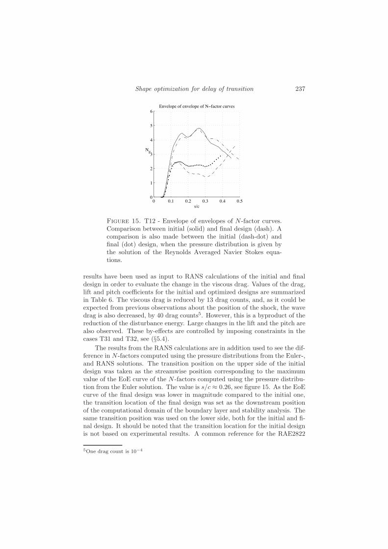
Shape optimization for delay of transition 237
0 0.1 0.2 0.3 0.4 0.50
1
2
3
4
5
6
NE
s/c
Envelope of envelope of N−factor curves
Figure 15. T12 - Envelope of envelopes of N -factor curves.Comparison between initial (solid) and final design (dash). Acomparison is also made between the initial (dash-dot) andfinal (dot) design, when the pressure distribution is given bythe solution of the Reynolds Averaged Navier Stokes equa-tions.
results have been used as input to RANS calculations of the initial and finaldesign in order to evaluate the change in the viscous drag. Values of the drag,lift and pitch coe"cients for the initial and optimized designs are summarizedin Table 6. The viscous drag is reduced by 13 drag counts, and, as it could beexpected from previous observations about the position of the shock, the wavedrag is also decreased, by 40 drag counts5. However, this is a byproduct of thereduction of the disturbance energy. Large changes in the lift and the pitch arealso observed. These by-e!ects are controlled by imposing constraints in thecases T31 and T32, see (§5.4).
The results from the RANS calculations are in addition used to see the dif-ference in N -factors computed using the pressure distributions from the Euler-,and RANS solutions. The transition position on the upper side of the initialdesign was taken as the streamwise position corresponding to the maximumvalue of the EoE curve of the N -factors computed using the pressure distribu-tion from the Euler solution. The value is s/c * 0.26, see figure 15. As the EoEcurve of the final design was lower in magnitude compared to the initial one,the transition location of the final design was set as the downstream positionof the computational domain of the boundary layer and stability analysis. Thesame transition position was used on the lower side, both for the initial and fi-nal design. It should be noted that the transition location for the initial designis not based on experimental results. A common reference for the RAE2822
5One drag count is 10!4

238 O. Amoignon, J. Pralits, A. Hanifi, M. Berggren & D. S. Henningson
RANS EulerCoe!. Case total viscous pressure pressure
Initial 2.3( 10"2 4.8( 10"3 1.8( 10"2 1.3( 10"2
CD T12 (Final) 1.6( 10"2 3.5( 10"3 1.3( 10"2 7.9( 10"3
T32 (Final) 1.8( 10"2 3.7( 10"3 1.4( 10"2 8.3( 10"3
Initial 8.4( 10"1 #7.9( 10"5 8.4( 10"1 8.4( 10"1
CL T12 (Final) 7.0( 10"1 #5( 10"5 7.0( 10"1 7.0( 10"1
T32 (Final) 8.5( 10"1 #7( 10"5 8.5( 10"1 8.5( 10"1
Initial 3.2( 10"1 # # 3.4( 10"1
CM T12 (Final) 2.4( 10"1 # # 2.6( 10"1
T32 (Final) 3.1( 10"1 # # 3.4( 10"1
Table 6. Summary of aerodynamic coe"cients at initial andfinal design for T12 and T32, using Euler and RANS flowanalysis.
airfoil is Cook & McDonald (1979), in which the boundary layer was tripped at3% chord in the experiments in order to have a well defined turbulent portion.
The pressure coe"cients obtained from the solution of the RANS for theinitial and final design is found in figure 14. The largest di!erence comparedto the Euler solution occur at the position of the shock wave. Upstream ofthis position however, the di!erence between the Euler and RANS solution issmaller, which can also be seen in figure 15, where the EoE curves of the twocases are compared. In the comparison of the pressure coe"cients between theEuler and RANS computations of the final design, one can note the di!erencein the region between x/c * 0.4 and x/c * 0.5. Results of the velocity fieldfrom the RANS calculation (not shown here), show that separation occurs inthis region. As this can not be accounted for in the boundary layer equationsused here, the EoE curve computed using the pressure distribution from theRANS calculation is not performed downstream of x/c * 0.4, see figure 15.
5.3.2. M# = 0.68, case T21
Results are shown here for the case of minimizing the disturbance kinetic energyof a single disturbance with the initial volume of the RAE2822 airfoil keptconstant. Computations are performed for Mach number M# = 0.68 at 0meter ASL. The shock wave shown in the T11-, and T12 cases is not presentin this case, see figure 17. The convergence history is given in figure 16. Theobjective function and the norm of the gradient are reduced of about threeorders of magnitude. The pressure coe"cients, and the geometries, at initialand final design, are found in figure 17. Alike the previous cases, the changes inthe geometry of the upper part of the airfoil influence the pressure distributionin a way that is favorable to decrease the disturbance energy. However, the

Shape optimization for delay of transition 239
0 2 4 6 8 10 12 14
10−8
10−7
10−6
10−5
10−4
E1
iteration
Objective function
0 2 4 6 8 10 12 14
10−7
10−6
10−5
10−4
10−3
||Gra
d||
iteration
Norm of gradient of objective function
Figure 16. T21 - Objective function and norm of its gradient.
0 0.2 0.4 0.6 0.8 1−1.5
−1
−0.5
0
0.5
1
1.5
−Cp
x/c
Pressure coefficients
0 0.2 0.4 0.6 0.8 1−0.08
−0.04
0
0.04
0.08
y/c
x/c
Airfoils
Figure 17. T21 - Pressure coe"cients and shapes at initial(solid) and final design (dash).
deformation of the airfoil is of a di!erent nature. Compared to the cases T11and T12, the upper part of the airfoil is thicker at final design than at initialdesign, which creates a region of higher curvature at about 40% of the chordlength away from the leading edge. This is further downstream compared towhere it appeared in the cases T11 and T12. The e!ects of these deformationscan be observed in changes of the pressure coe"cient.
The di!erence between the test cases is better understood looking at theenvelope of envelopes (EoE) curves of the N -factors. In case T11, the dist-urbances grow fastest in a region between x/c = 0.2 and x/c = 0.3, as seenin figure 12. In the case T21, the growth of disturbances continues increasing
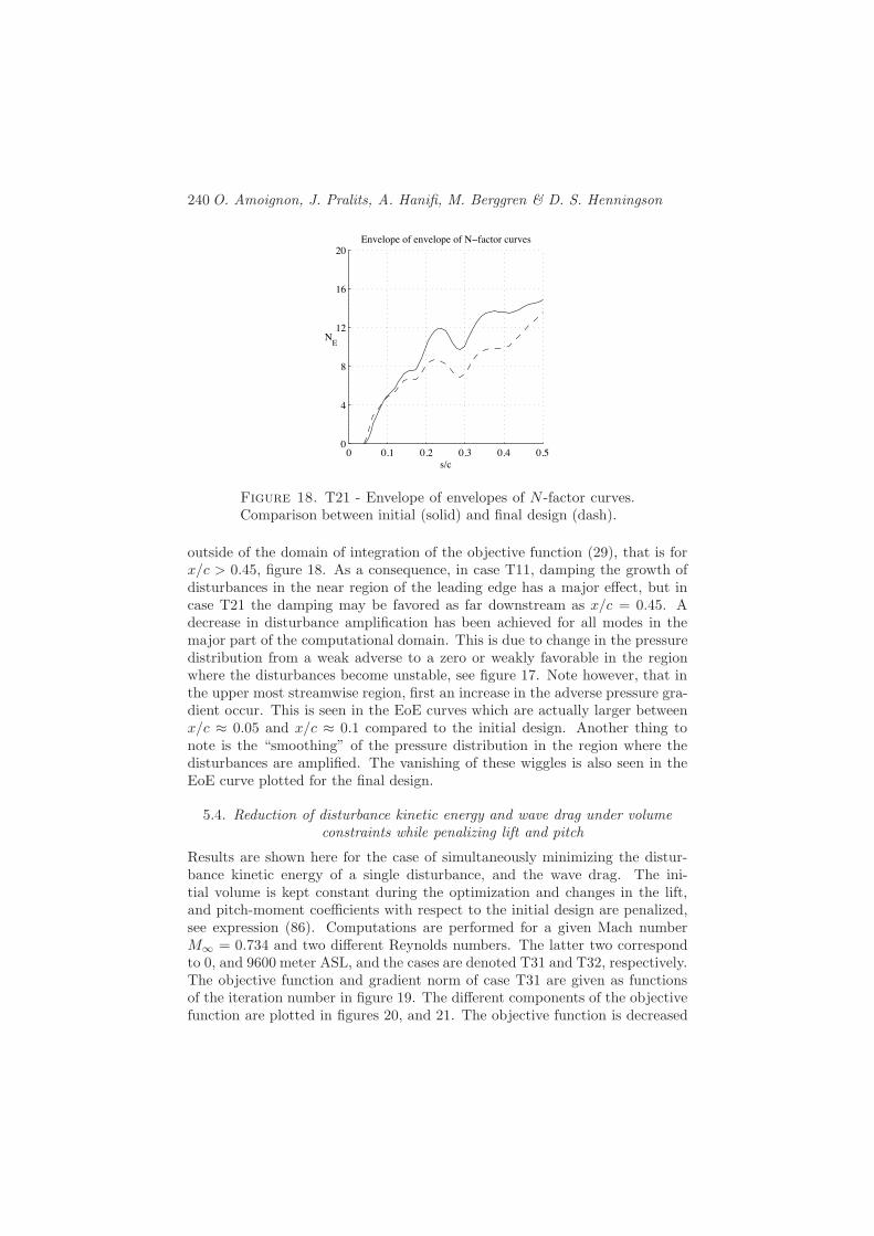
240 O. Amoignon, J. Pralits, A. Hanifi, M. Berggren & D. S. Henningson
0 0.1 0.2 0.3 0.4 0.50
4
8
12
16
20
NE
s/c
Envelope of envelope of N−factor curves
Figure 18. T21 - Envelope of envelopes of N -factor curves.Comparison between initial (solid) and final design (dash).
outside of the domain of integration of the objective function (29), that is forx/c > 0.45, figure 18. As a consequence, in case T11, damping the growth ofdisturbances in the near region of the leading edge has a major e!ect, but incase T21 the damping may be favored as far downstream as x/c = 0.45. Adecrease in disturbance amplification has been achieved for all modes in themajor part of the computational domain. This is due to change in the pressuredistribution from a weak adverse to a zero or weakly favorable in the regionwhere the disturbances become unstable, see figure 17. Note however, that inthe upper most streamwise region, first an increase in the adverse pressure gra-dient occur. This is seen in the EoE curves which are actually larger betweenx/c * 0.05 and x/c * 0.1 compared to the initial design. Another thing tonote is the “smoothing” of the pressure distribution in the region where thedisturbances are amplified. The vanishing of these wiggles is also seen in theEoE curve plotted for the final design.
5.4. Reduction of disturbance kinetic energy and wave drag under volumeconstraints while penalizing lift and pitch
Results are shown here for the case of simultaneously minimizing the distur-bance kinetic energy of a single disturbance, and the wave drag. The ini-tial volume is kept constant during the optimization and changes in the lift,and pitch-moment coe"cients with respect to the initial design are penalized,see expression (86). Computations are performed for a given Mach numberM# = 0.734 and two di!erent Reynolds numbers. The latter two correspondto 0, and 9600 meter ASL, and the cases are denoted T31 and T32, respectively.The objective function and gradient norm of case T31 are given as functionsof the iteration number in figure 19. The di!erent components of the objectivefunction are plotted in figures 20, and 21. The objective function is decreased

Shape optimization for delay of transition 241
0 2 4 6 8 10 12 140
0.04
0.08
0.12
0.16
0.2
JC
iteration
Objective function
0 2 4 6 8 10 12 14
10−2
10−1
100
101
||Gra
d||
iteration
Norm of gradient of objective function
Figure 19. T31 - Objective function and norm of its gradient.
in each step of the optimization even though the component of the wave dragis increased between iteration number 2 and 4, compared to iteration number1. The reason is that in this interval, the deviation of lift-, and pitch momentcoe"cients is decreased. A reduction has been obtained at the last iteration,in both disturbance kinetic energy and wave drag, while the lift-, and pitchmoment coe"cients are kept within a few percent. Comparisons between thepressure coe"cients, and geometries of the initial and final design are given infigure 22. The change in pressure distribution occurs mainly on the upper sideof the airfoil, where the shock wave has moved upstream and weakened. Incomparison with T11, which has the same initial conditions, the displacementof the shock in T31 is smaller, but, the changes in T31 reflect the conserva-tion of the pitch moment and lift coe"cients. The e!ect on the disturbancegrowth can be seen in figure 23 where the EoE curves have been plotted forthe initial and final design. A damping of the disturbance growth is obtainedin a large part of the computational domain using the final design. It is clearlooking at figure 22, that the adverse pressure gradient of the initial design inthe upstream region where the disturbances become unstable, has changed intoa zero or weakly favorable in the final design. Close to the shock wave of thefinal design, which has now moved further upstream, the flow is decelerated.This can be seen in the EoE curve where the value increases rapidly above thatof the initial design.
The convergence history for the lower Reynolds number case (T32) is foundin figures 24–26, and is similar to the one found for the case T31. The wavedrag experiences an increase during a few optimization steps also here, whilethe deviation of lift, and pitch-moment coe"cients decreases. In figure 27, acomparison is made between the pressure coe"cient and geometry of the initial

242 O. Amoignon, J. Pralits, A. Hanifi, M. Berggren & D. S. Henningson
0 2 4 6 8 10 12
10−1
100
101
E 1
iteration
Disturbance kinetic energy
0 2 4 6 8 10 12 1470
80
90
100
110
120
130
104 .C
D
iteration
Wave drag
Figure 20. T31 - Disturbance kinetic energy and wave drag.
0 2 4 6 8 10 12 140.2
0.3
0.4
0.5
0.6
0.7
0.8
0.9
iteration
Lift and pitch moment
Figure 21. T31 - Lift (triangle-solid) and pitch moment(circle-solid) coe"cients. The values at initial design are indi-cated at each step (solid).
and final design. In comparison with case T12, which has the same initial con-ditions, the displacement of the shock is smaller but the pressure distribution inT32 minimizes changes in the coe"cients of lift and pitch moment. The EoEcurves computed using the pressure distribution from the Euler solution areused, as in case T12, to set the transition locations in two RANS calculations.The transition position on the upper side of the initial design was taken as thestreamwise position of the maximum value of the EoE curve of the N -factorscomputed using the pressure distribution from the Euler solution (s/c * 0.26,

Shape optimization for delay of transition 243
0 0.2 0.4 0.6 0.8 1−1.5
−1
−0.5
0
0.5
1
1.5
−Cp
x/c
Pressure coefficients
0 0.2 0.4 0.6 0.8 1−0.08
−0.04
0
0.04
0.08
y/c
x/c
Airfoils
Figure 22. T31 - Pressure coe"cients and shapes at initial(solid) and final design (dash).
0 0.1 0.2 0.3 0.4 0.50
2
4
6
8
10
NE
s/c
Envelope of envelope of N−factor curves
Figure 23. T31 - Envelope of envelopes of N -factor curves.Comparison between initial (solid) and final design (dash).
see figure 28). The maximum value of the EoE curve computed for the final de-sign is below the value found for the initial one. The transition location on theupper side of the final design is therefore set as the downstream position of thecomputational domain of the boundary layer equations. The same transitionposition was used both for the initial and final design on the lower side. Themajor di!erences in the pressure distribution between the Euler and RANScalculation occur in the region around the shock wave. Upstream of the shockthe di!erence is smaller, both for the initial and final design. This can alsobe seen in the comparison of the EoE curves found in figure 28. A decrease

244 O. Amoignon, J. Pralits, A. Hanifi, M. Berggren & D. S. Henningson
0 2 4 6 8 10 12 14 160
0.04
0.08
0.12
0.16
0.2
JC
iteration
Objective function
0 2 4 6 8 10 12 14 16
10−2
10−1
100
101
||Gra
d||
iteration
Norm of gradient of objective function
Figure 24. T32 - Objective function and norm of its gradient.
occur in the N -factor values in both results showing the EoE curves of the finaldesign. This can be explained by the change in pressure gradient from adverseto zero or favorable, in a large part of the region where the disturbances areamplified.
0 2 4 6 8 10 12 14 16
10−2
10−1
100
E 1
iteration
Disturbance kinetic energy
0 2 4 6 8 10 12 14 1670
80
90
100
110
120
130
104 .C
D
iteration
Wave drag
Figure 25. T32 - Disturbance kinetic energy and wave drag.

Shape optimization for delay of transition 245
0 2 4 6 8 10 12 14 160.2
0.3
0.4
0.5
0.6
0.7
0.8
0.9
iteration
Lift and pitch moment
Figure 26. T32 - Lift (triangle-solid) and pitch moment(circle-solid) coe"cients. The values at initial design are indi-cated at each step (solid).
0 0.2 0.4 0.6 0.8 1−1.5
−1
−0.5
0
0.5
1
1.5
−Cp
x/c
Pressure coefficients
0 0.2 0.4 0.6 0.8 1−0.08
−0.04
0
0.04
0.08
y/c
x/c
Airfoils
Figure 27. T32 - Pressure coe"cients and shapes at initialdesign for Euler (solid) and RANS (dash-dot), and final designfor Euler (dash) and RANS (dot).
6. Summary and discussionTheory and results have been presented for an approach to perform shapeoptimization with the aim of transition delay, and thus a decrease of the viscousdrag. The location of laminar-turbulent transition is analyzed using linearstability theory, in which perturbations with infinitely small amplitude aresuperimposed on the laminar mean flow. It is then assumed that transition willoccur at the location where the total amplification of disturbances, with respect

246 O. Amoignon, J. Pralits, A. Hanifi, M. Berggren & D. S. Henningson
0 0.1 0.2 0.3 0.4 0.50
1
2
3
4
5
6
NE
s/c
Envelope of envelope of N−factor curves
Figure 28. T32 - Envelope of envelopes of N -factor curves.Comparison between initial (solid) and final design (dash). Acomparison is also made between the initial (dash-dot) andfinal (dot) design, when the pressure distribution is given bythe solution of the Reynolds Averaged Navier Stokes equa-tions.
to the first streamwise position where the disturbance starts to grow, attainsan empirically determined value, whose logarithm is generally denoted by N .The inviscid flow is obtained by solving the Euler equations for compressibleflows, and the viscous mean flow is obtained from the solution of the boundarylayer equations for compressible flows on infinite swept wings. The evolutionof convectively unstable disturbances is analyzed using the linear parabolizedstability equations (PSE).
In the present approach, an iterative gradient based optimization proce-dure is used with the aim of minimizing an objective function based on thedisturbance kinetic energy. Tests are carried out starting from the RAE2822airfoil and are formulated to produce a reduction of the disturbance kineticenergy while maintaining a fixed volume, angle of attack, region around theleading edge and trailing edge position. Flow conditions include transonic andsubsonic cases, with Reynolds number of 6.5, and 17 millions. In some casesthe objective function is formulated to simultaneously reduce the wave dragand the disturbance kinetic energy while maintaining lift and pitch momentcoe"cients near their values at initial design. The normal displacements of thenodes on the airfoil are solution of a quadratic programming problem minimiz-ing the variational form of the discrete Poisson problem and including linearconstraints. Such a parameterization ensures smoothness of the geometries foreach design generated by the quasi-Newton optimization algorithm (see Byrd1994) and enables to define complex sets of admissible shapes as needed whencoupling the three state equations. It has been shown that the gradient of the

Shape optimization for delay of transition 247
objective function with respect to the design variables can be evaluated fromthe solution of adjoint of the Euler, boundary layer and parabolized stabil-ity equations. Using the adjoint equations, as opposed to other perturbationtechniques, constitutes an e"cient way to evaluate functional gradients whenthe number of design variables is large compared to the number of objectivefunctions.
The work presented here is an ongoing project with improvements to bemade in order to increase the existing computational e"ciency and accuracy. Itis further possible to include additional physical modeling in order to generalizethe technique for more complex flow situations. As discussed herein, there areissues related to grid resolution and the approach taken to derive the adjointequations. From a physical point of view, in order to obtain a converged result,di!erent grid resolutions might be required for the Euler, boundary layer andstability equations. As shown here, the medium RAE2822 grid has a resolutionwhich is fine with respect to what is needed for the Euler solution and coarsewith respect to the stability solution. However, further refinement would notgive large improvements in the physical results. For the evaluation of the gra-dient of the disturbance kinetic energy with respect to the pressure distributionon the other hand, the resolution plays an important role, as the ABLE andAPSE are derived using the continuous approach. For this reason e!ort mustbe put into either deriving these equations using the discrete approach or toimprove on the interpolation technique shown here.
There are modifications which can be made in order to approach a morerealistic situation. One is to include the disturbance growth also on the lowerside of the wing in the objective function, as transition occurs on both sidesof the wing. As the objective function of the total disturbance kinetic energyis given as the sum of K convectively unstable disturbances, test can also bemade in order to evaluate this e!ect. Another extension, which can includeboth of the above, is to use multiple design points in the optimization. In suchcase the objective function is the sum of a chosen cost function at e. g. di!erentMach numbers and/or di!erent disturbances.
With the approach taken here there are some limitations which could beovercome using additional physical modeling. As no iterative coupling existbetween the pressure distribution and the thickness of the boundary layer, thisconstitutes an approximation. In addition, the boundary layer calculated hereis assumed laminar, and the e!ect of the increased thickness of the turbulentboundary layer due to transition is not accounted for. Separation is anotherissue which is not taken into account, and can be important especially forapplications with large angle of attack. Several studies have been made onthis topic for the boundary layer and stability analysis and might be possibleto include in the current project. Another option that should be tested inorder to avoid large adverse pressure gradients which might cause separationin the downstream domain, is to minimize an objective function including bothEK and Ef . The idea to include also the disturbance kinetic energy at a

248 O. Amoignon, J. Pralits, A. Hanifi, M. Berggren & D. S. Henningson
downstream position (Ef ), is based on the knowledge that an adverse pressuregradient has a destabilizing e!ect on the disturbance growth. Instead of usingthe Euler equations an extension is to use the Reynolds Averaged Navier-Stokesequations (RANS). This development should include the adjoint of the RANSequations.
Even though the Euler and adjoint Euler equations can be derived andsolved for complete three-dimensional flows, the boundary layer and stabilityequations used here are given for, at most, infinite swept wing flows. The ab-sence of variation of the viscous mean flow in the spanwise direction in the BLEand PSE means that e. g. tapered wings can not be analyzed without furtherapproximations. To proceed to fully three-dimensional cases, it therefore hasto be decided what approximations to make, or if e!ort should be spent onsolving the BLE and PSE for complete three-dimensional flows.
The delay of transition is a benefit if accounting for all other aerodynamicproperties of the wing, which are the wave drag, lift and moments coe"cients.Reducing the wave drag is as important as the delay of transition when opti-mizing the airfoil at cruise speed. The latter can be achieved by formulatingthe objective function as a weighted sum of the wave drag and the disturbancekinetic energy. Lift and pitch moment can also be maintained near to theirvalue for the initial design by adding terms to the objective function that pe-nalize variations of these coe"cients. However, in real life applications theinterest is to maintain the lift above a minimum level while fixing the momentsto their value at the original design. Imposing bound constraints in this nonlinear optimization problem would require to use more advanced method thanthe penalization technique that has been use in this study.
AcknowledgmentThe financial support of the EU project (ALTTA contract G4RD-CT-2000-00143) is gratefully acknowledged. Finally this research has received supportfrom the AEROSHAPE project funded by the European Commission, DG Re-search, under the GROWTH initiative (Project Ref: GRD1-1999-10752).
References
Airiau, C., Bottaro, A., Walther, S. & Legendre, D. 2003 A methodologyfor optimal laminar flow control: Application to the damping of Tollmien-Schlichting waves in a boundary layer. Phys. Fluids 15, 1131–1145.
Amoignon, O. 2003 Adjoint-based aerodynamic shape optimization. Licentiate thesisto be published, Department of Information Technology, Division of ScientificComputing, University of Uppsala.
Anderson, W. & Bonhaus, D. 1999 Airfoil design on unstructured grids for turbu-lent flows. AIAA Journal 37 (2), 185–191.
Shape optimization for delay of transition 249
Arnal, D. 1993 Boundary layer transition: Predictions based on linear theory. Spe-cial course on ’progress in transition modeling’, March-April 1993. AGARD-R-793, 2-1–2-63.
Barth, T. J. 1991 Aspects of unstructured grids and finite-volume solvers for theEuler and Navier–Stokes equations. In Special Course on Unstructured Methodsfor Advection Dominated Flows, pp. 6–1–6–61. AGARD Report 787.
Baysal, O. & Ghayour, K. 2001 Continuous adjoint sensitivities for optimizationwith general cost functionals on unstructured meshes. AIAA Journal 39 (1),48–55.
Berggren, M. 2003 Edge-based mesh movement strategies. Unpublished preprint,Sandia National Laboratories.
Bertolotti, F. P., Herbert, T. & Spalart, S. 1992 Linear and nonlinear stabilityof the Blasius boundary layer. J. Fluid Mech. 242, 441–474.
Burgreen, G. 1994 Improving the e"ciency of aerodynamic shape optimization.AIAA Journal 32 (1), 69–76.
Byrd, R. 1994 A limited memory algorithm for bound constrained optimization.Tech. Rep. NAM-08. Northwestern University, Department of Electrical Engi-neering and Computer Science, Evanston Il 60208.
Byrd, R., Lu, P., Nocedal, J. & Zhu, C. 1995 A limited memory algorithm forbound constrained optimization. SIAM J. Sci. Comput. 16, 1190–1208.
Cook, P. & McDonald, M.A.and Firmin, M. 1979 Aerofoil RAE 2822 – pressuredistributions, and boundary layer and wake measurements. Experimental database for computer program assessment. AGARD-AR-138, a6.
Eliasson, P. 2001 Edge, a Navier–Stokes solver, for unstructured grids. Tech. Rep.FOI-R–0298–SE. Swedish Defence Research Agency, Stockholm.
Elliot, J. 1998 Aerodynamic based on the Euler and Navier–Stokes equations usingunstructured grids. PhD thesis, MIT Dept. of Aero. and Astro.
Enoksson, O. 2000 Shape optimization in compressible inviscid flow. Licenciate The-sis LiU-TEK-LIC-2000:31, institute of Technology, Lindkpings University, Dept.of Math., ISBN 91-7219-780-3 ISSN 0280-7971.
Frank, P. & Shubin, G. 1992 A comparison of optimization-based approaches for amodel computational aerodynamics design problem. Journal of ComputationalPhysics 98, 74–89.
Giles, M. & Pierce, N. 2000 An introduction to the adjoint approach to design.Flow, Turbulence and Control 65, 393–415.
Green, B. E. & Whitesides, J. L. 1996 A method for the constrained design ofnatural laminar flow airfoils. AIAA Paper (96-2502).
Hanifi, A., Henningson, D. S., Hein, S. & Bertolotti, F. P.and Simen, M.1994 Linear non-local instability analysis - the linear NOLOT code. FFA TN1994-54.
Herbert, T. 1997 Parabolized stability equations. Annu. Rev. Fluid Mech. 29, 245–283.
van Ingen, J. L. 1956 A suggested semiempirical method for the calculation of theboundary layer transition region. Tech. Rep. VTH-74. Department of Aeronau-tical Engineering, University of Delft.
Jameson, A. 1988 Aerodynamic design via control theory. Journal of Scientific Com-puting 3, 233–260.

250 O. Amoignon, J. Pralits, A. Hanifi, M. Berggren & D. S. Henningson
Jameson, A. 1997 Optimum aerodynamic design using the Navier-Stokes equations.AIAA Paper no 97-0101 35th Aerospace Sciences Meeting and Exhibit., Reno,Nevada.
Joslin, R. 1998 Overview of laminar flow control. Tech. Rep. 1998-208705. NASA,Langley Research Center, Hampton, Virginia.
Lee, J.-M., Schrage, D. P. & Mavris, D. N. 1998 Development of subsonic trans-ports with laminar flow wings. AIAA Paper (98-0406).
Lighthill, M. J. 1945 A new method of two-dimensional aerodynamic design. Tech.Rep.. ARC, rand M 2112.
Lions, J. 1971 Optimal Control of Systems Governed by Partial Di!erential Equa-tions. Springer-Verlag,New York, translated by S.K. Mitter.
Malik, M. R. 1989 Prediction and control of transition in supersonic and hypersonicboundary layers. AIAA J. 27, 1487–1493.
Malik, M. R. & Balakumar, P. 1992 Nonparallel stability of rotating disk flowusing PSE. In Instability, Transition and Turbulence (ed. M. Hussaini, A. Kumar& C. Streett), pp. 168–180. Springer.
Manning, V. M. & Kroo, I. M. 1999 Multidisciplinary optimization of a naturallaminar flow supersonic aircraft. AIAA Paper (99-3102).
Mohammadi, B. 1997 A new optimal shape procedure for inviscid and viscous tur-bulent flows. Int. J. Numer. Meth. Fluids 25, 183–203.
Nocedal, J. & Wright, S. 1999 Numerical Optimization. Springer Series in Oper-ations Research, iSBN:0-387-98793-2.
Pironneau, O. 1973 On optimal profiles in Stokes flow. J. Fluid Mech. 59, 117–128.
Pralits, J. O. 2001 Towards optimal design of vehicles with low drag: Applicationsto sensitivity analysis and optimal control. Licentiate thesis KTH/MEK/TR-01/07. Royal Institute of Technology, SE-172 90 Stockholm, Sweden.
Pralits, J. O., Airiau, C., Hanifi, A. & Henningson, D. S. 2000 Sensitivity anal-ysis using adjoint parabolized stability equations for compressible flows. Flow,Turbulence and Combustion 65, 321–346.
Pralits, J. O. & Hanifi, A. 2003 Optimization of steady suction for disturbancecontrol on infinite swept wings. Phys. Fluids 15 (9).
Pralits, J. O., Hanifi, A. & Henningson, D. S. 2002 Adjoint-based optimizationof steady suction for disturbance control in incompressible flows. J. Fluid Mech.467, 129–161.
Reuther, J. 1999 Constrained multipoint aerodynamic shape optimization using anadjoint formulation and parallel computers, part 1. J. Aircraft 36 (1), 51–60.
Schubauer, G. B. & Skramstad, H. K. 1948 Laminar-boundary-layer oscillationsand transition on a flat plate. NACA Tech. Note No. 909 .
Simen, M. 1992 Local and non-local stability theory of spatially varying flows. InInstability, Transition and Turbulence (ed. M. Hussaini, A. Kumar & C. Streett),pp. 181–201. Springer.
Smith, A. M. O. & Gamberoni, N. 1956 Transition, pressure gradient and stabilitytheory. Tech. Rep. ES 26388. Douglas Aircraft Co.
Soemarwoto, B. 1996 Multi-point aerodynamic design by optimization. PhD thesis,Delft University of Technology, Faculty of Aerospace Engineering, P.O. Box 5058,2600 GB Delft, Netherlands, iSBN 90-5623-051-4.

251
Sung, C. & Kwon, J. 2000 Accurate aerodynamic sensitivity analysis using adjointequations. AIAA Journal 38 (2), 243–250.
Wallin, S. & Johansson, A. V. 2000 An explicit algebraic Reynolds stress modelfor incompressible and compressible turbulent flows. J. Fluid Mech. 403, 89–132.
Zhu, C., Byrd, R., Lu, P. & Nocedal, J. 1994 L-BFGS-B: Fortran subroutinesfor large scale bound constrained optimization. Tech. Rep. NAM-11. EECS De-partment, Northwestern University.
Zurigat, Y. H., Nayfeh, A. H. & Masad, J. A. 1990 E!ect of pressure gradienton the stability of compressible boundary layers. AIAA Paper (90-1451), 21stFluid Dynamics, Plasma Dynamics and Lasers Conference, Seattle, WA.