Optimal design of elastic columns formaximum buckling load

Dragan T. SpasicUniversity of Novi Sad, YugoslaviaE-mail: spasic@uns.ns.ac.yu

Abstract

The problem of Lagrange, to �nd the curve which by its revolution about an axisin its plane determines the column of greatest e¢ ciency, is examined. A comparisonis made between the optimal shapes of the compressed column predicted by severalexisting formulations for columns of circular cross section hinged at the end points.Then, two di¤erent generalizations of the problem, that follow from a generalizedplane elastica and the theory called Kirchho¤�s kinetic analogue, are considered.The optimal shape of a compressed column that can su¤er not only �exure as inclassical elastica theory, but also compression and shear is �rst presented. Second,the distribution of material along the length of a compressed and twisted columnis optimized so that the column is of minimum volume and will support a givenload without spatial buckling. Necessary conditions for both problems are derivedusing the maximum principle of Pontryagin. The optimal shapes are obtained bynumerical integration. The principal novelty of the present results is that bothsolutions, that follow from two possible generalizations of the classical Bernoulli-Euler bending theory, lead to the optimum column with non-zero cross sectionalarea at its ends.

1 Introduction

The problem of determining that shape of compressed column which has the largest Eulerbuckling load was posed by Lagrange in 1773. Clausen in 1851 solved it for columns ofcircular cross section pined at the end points. Although that result was mathematicallycorrect the obtained optimal shape did have points where the cross section vanishes.Nikolai [1], in work long unnoticed outside the Soviet Union, was the �rst author whoconsidered that anomaly of Clausen�s solution. In order to avoid any �nite load to inducein�nite stresses in the column, Nikolai proposed minimal cross sectional area at the ends,determined so that given limiting stress will not be exceeded. Since then, many results ofstructural optimization could be related to the problem of Lagrange. Mathematically, thisamounts to maximizing an eigenvalue of a certain Sturm-Liouville system to obtain anisoperimetric inequality. It is worth noting that the problem of Lagrange with clamped-clamped boundary conditions, was attacked in 1962 by Tadjbakhsh and Keller [2] in thecontinuation of work Keller [3] had begun at the suggestion of Cli¤ord Truesdell. That

1

case, in which the column is clamped at each end, seems to be especially troublesomesince the solution has two points in its interior where the cross sections vanishes.It is obvious that these extremal shapes have led to confusion and several attempts

to resolve the anomaly. Nearly in the same manner as Nikolai, Trahair and Booker [4]have considered the problem of avoiding the zero cross sectional area at the end of theoptimal column. In 1977 Olho¤ and Rasmussen [5] noted what�s wrong in Tadjbakhshand Keller�s work. Also they presented bimodal formulation of the column problem.Namely, structural optimization combines mathematics and mechanics with engineeringand has become a broad multidisciplinary �eld, see Prager and Taylor [6], Rozvany andMroz [7] and Vanderplaats [8]. The constant �ow of general reviews, surveys of sub�eldsand conference proceedings on optimal design testify the strong activity and increasingimportance of the �eld, see Olho¤ and Taylor [9] as a source for additional bibliography.We note that the problem of Lagrange and the optimal shapes for which the cross sectionsvanishes at certain points were reconsidered many times, see results of Barnes [10], [11],Seiranian [12], Plaut et al. [13] and Cox and Overton [14]. Now it is clear that all theseresults are mathematically correct. Also it is remarkable that these results were based onthe linear equilibrium equations that follow from Bernoulli-Euler bending theory as thesimplest model for the planar �exure of an elastic column described by an inextensiblecurve constrained to lie in plane.Optimization of columns for maximum buckling load still remains a topic of wide-

spread interest. In what follows, the problem of Lagrange is generalized in two directions.First, the optimal shape of compressed column that can su¤er not only �exure as in theclassical elastica theory, but also compression and shear will be considered. Also, byuse of Kirchho¤�s kinetic analogue, see Antman and Kenney [15], the optimal shape ofcompressed and twisted column against spatial buckling will be determined. We shallshow that both solutions that follow from these two possible generalizations of the clas-sical Bernoulli-Euler elastica theory lead to the optimum columns with non-zero crosssectional area at the ends. Namely, according to Clausen�s solution the optimum columnhas zero cross sectional area at the ends, and therefore, roughly speaking, at the ends doesnot recognize the di¤erence between any applied �nite load and, for example, its doubledvalue. It seems that Clausen�s solution will never �t for real columns. In consideringNikolai�s work [1] and his comments on that solution, three points should be noted. First,the condition that limiting stress should be included in the column problem is taken fromthe linear theory called strength of materials. Secondly, it was implicitly allowed thatthe strongest column will change its length under compression. Thus, Nikolai�s solutioncould not be considered within Bernoulli-Euler beam theory because the classical theoryof buckling neglects axial strain of the central line as a possible deformation of an elas-tic rod. Lastly, although according to Gjelsvik [16], the �rst work that generalizes theclassical elastica theory as to take the shearing forces into account goes back to Engesser,who considered the in�uence of shear on the buckling loads in 1889, in the problem ofLagrange the in�nite value of shear rigidity was assumed.The aim of any theory of rods or beams is to describe the deformed con�guration

of a slender three-dimensional body by a single curve and certain parameters recordingmaterial orientation relative to that curve, see Parker [17]. The three-dimensional elasticconstitutive law is replaced by expressions for resultant forces, moments and generalized

2

moments in terms of extension, curvatures, torsion and the remaining parameters. Eachresulting theory must necessarily be approximate, although its accuracy should increaseas the representative scale of distance along the axis of the rod increases relative to atypical diameter of the cross section. According to that lines we �nd that Clausen�ssolution is correct in sense of the classical Bernoulli-Euler elastica theory, and if we wouldlike to improve it to �t for real columns we are to pose the column problem within ageneralized plane elastica theory. In doing that both e¤ects, shear and compressibility,should be taken into account. Namely, it is a well known fact that the Euler buckling loadis sensitive of both e¤ects. In other words, decreasing of shear rigidity of the column thevalue of the Euler buckling load decreases, and the decreasing of the extensional rigiditythe value of critical load increases. Thus, in the �rst part we intend to consider e¤ects ofshear and compressibility on the optimal shape of the compressed column.The next problem, we consider here, is motivated by Keller�s work [3] and is suggested

by adopting a slightly di¤erent generalization of the classical Bernoulli-Euler elastica.With a plausible generalization of the column load that leads to spatial buckling weintend to make another study of the Lagrange problem. We shall add twisting couples atthe ends of the column for which, once again, the in�nite values for shear and extensionalrigidity will be assumed. Namely, Grenhhill in 1883 studied the buckling of a columnunder terminal thrust and torsion, and determined Euler buckling load for the columnof uniform circular cross section, see Love[18]. For that load the distribution of materialalong the length of compressed and twisted column will be optimized so that the columnwill be of minimum volume and will support a given load without spatial buckling.In order to motivate the approach to be followed, let us recall formulations presented

in papers Chung and Zung [19] and Bratus and Zharov [20]. Also, we shall recall Pearson�sformulation of Lagrange problem [14], that is, to �nd the curve which by its revolutionabout an axis in its plane determines the column of great e¢ ciency, and note that e¢ ciencyhere denotes structure�s resistance to buckling under axial compression. In what followsonly a symmetric buckling mode within the classical Bernoulli-Euler elastica theory willbe considered. Necessary conditions for optimal control problems we treat here will bederived using the maximum principle of Pontryagin, see Kirk [21] or Alekseev et al. [22].The optimal shapes will be obtained by numerical integration.Let us consider a slender column represented in rectangular Cartesian coordinate sys-

tem Ozx by a plane curve C of a given length L as shown in Figure 1. The curve Crepresents the column axis which coincides with the centroidal line of the column crosssections. In order to deal with a well de�ned problem we assume that the column is hingedat either end, the hinge at the origin O being �xed whereas the other one is free to movealong the axis z: We assume that the column is loaded by a concentrated force F havingthe action line along the z axis which coincide with the column axis in the undeformedstate. Namely, Figure 1 shows the deformation of the column under its buckling load.We denote the bending rigidity of the column and the angle between the tangent to thecolumn axis and the z axis with EI = EI (S) and = (S) respectively. Here S denotesthe arc length of C measured from one end point. Implicitly it is assumed here thatextensional and shear rigidity are in�nite.

3

Figure 1. Hinged column under buckling load.

We note that according to Pearson�s formulation, the column is of circular cross sec-tion, of area A = A (S) ; so that either EI (S) or A (S) determines the distribution ofmaterial along the length of a column. For a uniform column these values are EIo andAo respectively.The half volume of the column is

V =

L=2Z0

A (S) dS: (1)

It is well known fact that the equilibrium con�guration of the column is given by thefollowing di¤erential equations

x0 = sin ; z0 = cos ; 0 = �FxEI

; (2)

where (�)0 = d (�) =dS; and the following boundary conditions

x (0) = 0; z (0) = 0; (L=2) = 0: (3)

Also, the critical load for the case of compressed column of uniform cross section boundedas shown in Figure 1 is

Fc =�2EIoL2

; (4)

for example see Love [18]. Note that z variable can be omitted from the following analysis.We introduce now the following non-dimensional quantities

t =S

L; � =

x

L; a =

A

Ao; v =

V

AoL; � =

FL2

EIo; (5)

and note

EI

EIo=

EA2

4�EA2o4�

= a2:

Then Eqs. (1), (2) and (3) become

v =

Z 1=2

0

adt; (6)

4

_� = sin ; _ = ���a2; (7)

� (0) = 0; (1=2) = 0: (8)

where:

(�) = d (�) =dt: From now on we choose a = a (t) to be the non-dimensional para-meter that determines the distribution of material along the column axis.Now, following the lines of the above papers [19], [20] the column�s resistance to buck-

ling under axial compression as a problem of optimal control theory could be expressed,at least in three di¤erent ways:I) to �nd the distribution of material along the length of a column so that the column

is of minimum volume and will support a given load without buckling, in our notation,reads

minav;

_� = ; _ = ���a2; (9)

� (0) = 0; (1=2) = 0;

II) to �nd the distribution of material along the length of a column of a given volumewhich will give the largest possible buckling load, i.e.

maxa�;

_� = ; _ = ���a2; _v = a; _� = 0; (10)

� (0) = 0; (1=2) = 0; v (0) = 0; v (1=2) = vp;

where vp is that given volume, andIII) to �nd the distribution of material along the length of a column of a given volume

which will give the largest possible load provided given postbuckling deformation will notbe exceeded, i.e.

maxa�;

_� = sin ; _ = ���a2; _v = a; _� = 0; (11)

� (0) = 0; (1=2) = 0; v (0) = 0; v (1=2) = vp; � (1=2) = �p;

where �p is given as the maximum de�ection of the column in the post-critical region.We note that in the third formulation the nonlinear equilibrium equations are used.

Also for small values of �p the second and the third formulation coincide. In solvingproblems given by Eqs. (9) - (11) Pontryagin�s maximum principle is used. According tothat principle, necessary conditions for optimality, Euler-Lagrange or costate equations,and natural boundary conditions for the problems (9) - (11) respectively, [21], [22], readI)

a = 3p�2��p ;

_p� =�p a2

; _p = �p�;

p� (1=2) = 0; p (0) = 0;

(12)

5

II)

a = 3

r�2��p pv

;

_p� =�p a2

; _p = �p�; _pv = 0; _p� =p �

a2;

p� (1=2) = 0; p (0) = 0; p� (0) = 0; p� (1=2) = 1;

(13)

III)

a = 3

r�2��p pv

;

_p� =�p a2

; _p = �p� cos ; _pv = 0; _p� =p �

a2;

p (0) = 0; p� (0) = 0; p� (1=2) = 1;

(14)

where Lagrange multipliers p�; p ; pv and p� and the corresponding Hamiltonians areintroduced in the usual way. It is obvious that condition p (0) = 0 always implies thatthe cross section vanishes at the end of the column, i.e.,

a (0) = 0: (15)

Although the obtained problems given by Eqs. (9), (10) and (11) with Eqs. (12),(13) and (14), respectively, could be solved in closed form, as in papers [19], [20], toget the optimal shapes against buckling we shall use numerical methods presented inPress et al. [23]. The shooting method is of course a standard technique for solvingtwo point boundary value problems. First we shall examine the optimal column and theuniform column of the same volume. Then, results for the optimal shape obtained fromthe �rst problem,with results obtained from the second, and the third formulation, willbe compared.If we consider the buckling load of the slender column of unit length and unite volume

with uniform distribution of the material along the column axis, i.e., the critical load�c = �2 = 9:869; than the obtained minimum half volume of the optimal column isvmin = 0:433: In Figure 2 the optimal shape, as a solution of the problem given by Eqs.(9) and (12) is presented. Namely, instead of the solution of the �rst problem given byEqs. (9) and (12), say a = aopt (t) ; in Figure 2 we present optimal curve obtained asRopt (t) =

paopt (t); which according to Pearson formulation, gives the column of greatest

e¢ ciency. The obtained shape corresponds to Clausen�s solution of Lagrange problem.The uniform column of the same volume as the optimal one with corresponding constantradius of the cross section R1 = 0:93 < 1 is also shown.

6

Figure 2. Clausen�s solution and uniform column.

In order to examine the postbuckling behavior of the column of unit length and thehalf volume v1 = 0:433 with uniform cross section �rst, we note that its buckling load is�1 = 7:402 < �c: Further, we solve two point boundary value problem given by Eqs. (7),(8) with � = �c and a21 = 0:75: In Figure 3 the post-critical shape of the curve C for theuniform column of half volume v1 = 0:433 is shown.

Figure 3. Postcritical shape of the uniform column.

We note very large de�ection of the uniform column axis. When compared with theuniform column, the optimal column loaded with � = �c still remains straight. It maybe added that the optimal shapes for the �rst and the second formulation are the same.Namely, if we choose vp = 0:433 and solve the second problem given by Eqs. (10) and (13)we get �max = �2 as expected. Thus, the �rst and the second formulation are equivalent,but the �rst one is easier to tackle. Also, if we put the value that corresponds to thecolumn of unit length and unite volume, vp = 0:5; from the second problem we obtain�max = 13:159: Similarly, with value � = 13:159 according to the �rst formulation theminimum half volume of the optimal column equals vmin = 0:5:To investigate the agreement of the second and the third solution �rst we need to

examine the value �p. In Bratus and Zharov [20], where instead of �p = � (1=2) the value (0) is proposed, very large de�ections in post buckling region are allowed. Some ofthem are even bigger then the half length of the column. A �rst observation is that inengineering we intend to keep column in trivial - straight position so we propose here thevalues of �p to be not more than 15% of the column length. If we solve the third problemgiven by Eqs. (11) and (14) with vp = 0:5 and �p = 0:102 we get �max = 13:425: Asexpected the decreasing of the value �p the closeness of the second and the third solutionincreases. For example, with vp = 0:5 and �p = 0:05 we get �max = 13:221: Also we �nd

7

that the di¤erence between solution for aopt (t) obtained from the second (linear) problem,and the corresponding solution of the third (nonlinear) problem, is less then 10�2:In conclusion of this section we claim that among the equivalent problems the �rst

one is optimal for engineering applications. Namely, the previous analysis shows thatthe �rst formulation corresponds to the problem of minimum dimension. Also, the �rstformulation is based the linear equilibrium equations. We note that, the considerationsconcerning boundary condition �p in the third one will motivate our approach in spatialbuckling problem. Our next step is to analyze the column problem within a generalizedplane elastica theory with axial and shear deformations.

2 The plane problem

In the analysis that follows we shall examine the problem of Lagrange with the generalizedconstitutive equations given in Atanackovic and Spasic [24]. In other words, we intendto consider the same load con�guration and the symmetric buckling mode as shown inFigure 1, but now with �nite values for extensional and shear rigidity. As before we assumethat the column is straight in unload state. First, we shall derive nonlinear equilibriumequations. Then we shall show that the bifurcation points of the nonlinear equilibriumequations are determined by the eigenvalues of the linearized equations. Finally, we shalldetermine the optimal shape for the column model based on simple shear of �nite amount[24].

2.1 Di¤erential equations and boundary conditionsAn element of the column axis whose length in the undeformed state is dS in the deformedstate has the length ds.

Figure 4. Geometry of the deformed column element and components of the contactforce.

From Figure 4 we get the equilibrium equations for an element of length ds in thedeformed state

dH = 0; dW = 0; (16)

dM = Wdz �Hdx; (17)

where H and W are z and x components of the resultant force respectively, M is theresultant couple, z and x are the coordinates of an arbitrary point on the column in thedeformed state. The strain of the central axis is de�ned as

" =ds� dS

dS: (18)

8

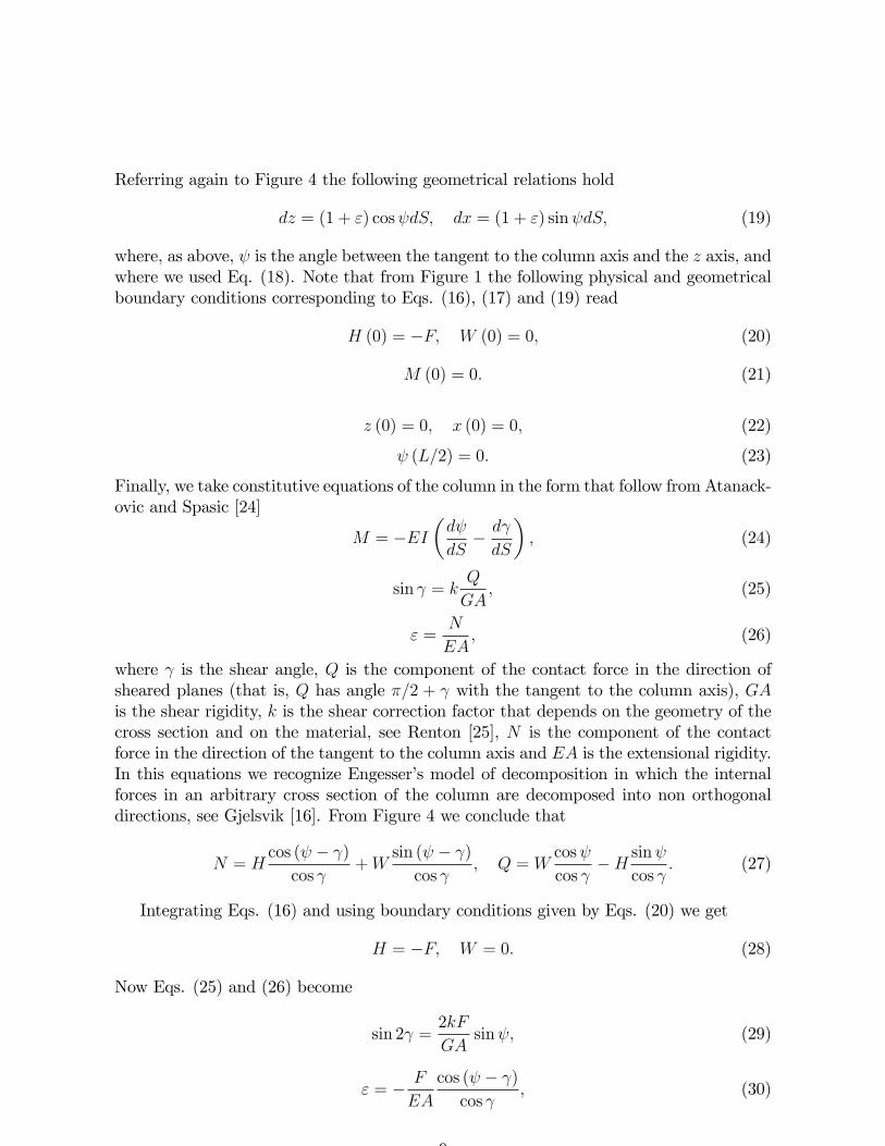
Referring again to Figure 4 the following geometrical relations hold

dz = (1 + ") cos dS; dx = (1 + ") sin dS; (19)

where, as above, is the angle between the tangent to the column axis and the z axis, andwhere we used Eq. (18). Note that from Figure 1 the following physical and geometricalboundary conditions corresponding to Eqs. (16), (17) and (19) read

H (0) = �F; W (0) = 0; (20)

M (0) = 0: (21)

z (0) = 0; x (0) = 0; (22)

(L=2) = 0: (23)

Finally, we take constitutive equations of the column in the form that follow from Atanack-ovic and Spasic [24]

M = �EI�d

dS� d

dS

�; (24)

sin = kQ

GA; (25)

" =N

EA; (26)

where is the shear angle, Q is the component of the contact force in the direction ofsheared planes (that is, Q has angle �=2 + with the tangent to the column axis), GAis the shear rigidity, k is the shear correction factor that depends on the geometry of thecross section and on the material, see Renton [25], N is the component of the contactforce in the direction of the tangent to the column axis and EA is the extensional rigidity.In this equations we recognize Engesser�s model of decomposition in which the internalforces in an arbitrary cross section of the column are decomposed into non orthogonaldirections, see Gjelsvik [16]. From Figure 4 we conclude that

N = Hcos ( � )

cos +W

sin ( � )

cos ; Q = W

cos

cos �H

sin

cos : (27)

Integrating Eqs. (16) and using boundary conditions given by Eqs. (20) we get

H = �F; W = 0: (28)

Now Eqs. (25) and (26) become

sin 2 =2kF

GAsin ; (29)

" = � F

EA

cos ( � )

cos ; (30)

9

where we used Eq. (27). From Eq. (29) we can express in terms of

=1

2arcsin

�2kF

GAsin

�: (31)

Now we de�ne a new variable� = � ; (32)

or

� = � 12arcsin

�2kF

GAsin

�; (33)

and note that the application of the implicit function theorem to Eq. (33) ensures theexistence of the following relation

= f (�) ; (34)

at least near zero. Then Eqs. (24) and (17) become

M 0 = F

0BB@1� F

EA

cos�

cos

�12arcsin

�2kF

GAsin f (�)

��1CCA sin f (�) ; �0 = �M

EI; (35)

where (�)0 = d (�) =dS. The boundary conditions corresponding to Eqs. (35) are

M (0) = 0; � (1=2) = 0; (36)

where we used Eqs. (23), (29) and (32). Now the equilibrium con�guration of the columnis described.The linearized boundary value problem corresponding to Eqs. (35), (36) leads to

equations

M 0 = F1� F

EA

1� kF

GA

�; �0 = �M

EI; (37)

with boundary conditions (36). Namely, if we linearize Eq. (29) we get

=kF

GA ;

and now Eq. (34) becomes

=1

1� kF

GA

�:

We note that for EA; GA ! 1; we could easily get the linearization of equilibriumequations for the classical column model given by Eqs. (2) and (3).

10

2.2 Bifurcation of the trivial solutionTo determine the critical load for the uniform column with constant cross section of areaAo; we shall use the methods presented in Krasnosel�skii et al. [26]. Namely, to prove thateigenvalues of the linearized problem determine bifurcation points of the nonlinear equi-librium equations we shall use the fact that the eigenvalues of the linearized equilibriumequations are stable in a specially de�ned sense.First, we note that variables z and x can be omitted from bifurcation analysis since

they could be determined after we �nd � (S) and then (S) and (S) : Then, we addmore the non-dimensional quantities to Eqs. (5). Namely, we introduce

� =kF

GAo; � =

F

EAo; m =

ML

EIo; (38)

and note that the nonlinear equilibrium equations of the uniform column with correspond-ing boundary conditions could be written in the following form

_m = �

(1� �

cos�

cos�12arcsin [2� sin f (�)]

) sin f (�) ; _� = �m; (39)

m (0) = 0; � (1=2) = 0; (40)

where:

(�) = d (�) =dt and where we used Eqs. (38) and (5). For all values of � system (39)with boundary conditions (40) admits a trivial solution

m � 0; � � 0;

in which the column axis remains straight, see Eq. (32) as well as Eq. (29). Namely,we treat � as the bifurcation parameter; that is, we �x F , L; EAo, and GAo and allowbending rigidity EIo to vary. Our next goal is to �nd the smallest value of �, denotedby �cg for which boundary value problem (39), (40) has non-trivial solution. Concerningthat system we note that the right hand sizes of Eqs. (39) do have continuous derivativeswith respect to m and � for t 2 [0; 1] ; m and � bounded, say m2 + �2 < �2 2 R+; for� > 0; and do vanishes on the trivial solution.The linearized boundary value problem corresponding to Eqs. (39), (40) reads

_m = �1� �

1� ��; _� = �m; (41)

with boundary conditions (40). In system (41) we used Eqs. (37), (38) and (5). Wetransform Eqs. (41) to

�m+ �2m = 0;

where �2 = � (1� �) = (1� �) ; and then �nd the solution of the linearized problem (41)in the following form

m = Dn sin�nt; � =D cos�nt

kn; n = 1; 2; ::: (42)

11

where Dn are constants and where we used the �rst boundary condition (38). The condi-tion that determines the critical load in sense of generalized elastica, �cg reads

cos�

2= 0 = cos

�

2;

so we get

�cg = �2(1� �)

(1� �): (43)

We note that for � = � = 0; we recover the classical critical load �cg = �c as expected.Also, for � = 0 we recover the result of Gjelsvik [26]. From Eq. (43) we see the wellknown fact that shear and compressibility have the opposite in�uence on Euler bucklingload. According to Renton [25], here and in all numerical examples that follows, for realcolumns we shall assume that � < 1 and that � is greater then �.Finally, to prove that the eigenvalues of linearized equations (41), (40) determine

the bifurcation points of nonlinear equations (39), (40) it is necessary to show that theeigenvalues of (41), (40) are stable in a specially de�ned sense, see Krasnosel�skii et al.[26]. To recognize the stable eigenvalue, say �s, �rst we de�ne a function � (t; �) byrelation

tan� (t; �) =� (t; �)

m (t; �);

where m (t; �) and � (t; �) are given by Eqs. (42). Then we require the condition

d [� (1=2; �)]

d�j�=�s 6= 0;

to be satis�ed. Namely, the condition that the function � (1=2; �) does not attain its localextremum at �s ensures the stability of an eigenvalue in the sense of Krasnosel�skii et al.[26]. For n = 1, �cg given by Eq. (43) and for m and given by Eqs. (42) that derivativereads

d [� (1=2; �)]

d�j�=�cg = �

1

4

�1 + ��2 (�1 + �) 6= 0:

This analysis con�rms that bifurcation takes place at the characteristic values of linearizedequations.We make two remarks here. First, the proof that the eigenvalues of the linearized

equilibrium equations (41), (40) are bifurcation points of the full nonlinear equilibriumequations (39), (40) could also proceed as either on applying the standard procedureof Liapunov-Schmidt reduction, see Chow and Hale [27] and Troger and Steindl [28] oron rewriting the governing di¤erential equations as an integral equation and on applyingdegree theoretic arguments of local bifurcation theory, see Antman and Rosenfeld [29] andHutson and Pym [30]. Both procedures assert that if the multiplicity of a characteristicvalue of linearized problem is odd, bifurcation does indeed take place. Second, notethat instead of Engesser�s model we could use either Haringx�s or Timoshenko type ofdecomposition, see Atanackovic [31]. Namely, the linearized form of Eqs. (24) - (26) willbe the same but Eqs. (27) will di¤er because the resultant force could be decomposed ineither the direction of the shared cross section and into the direction normal to the sheared

12

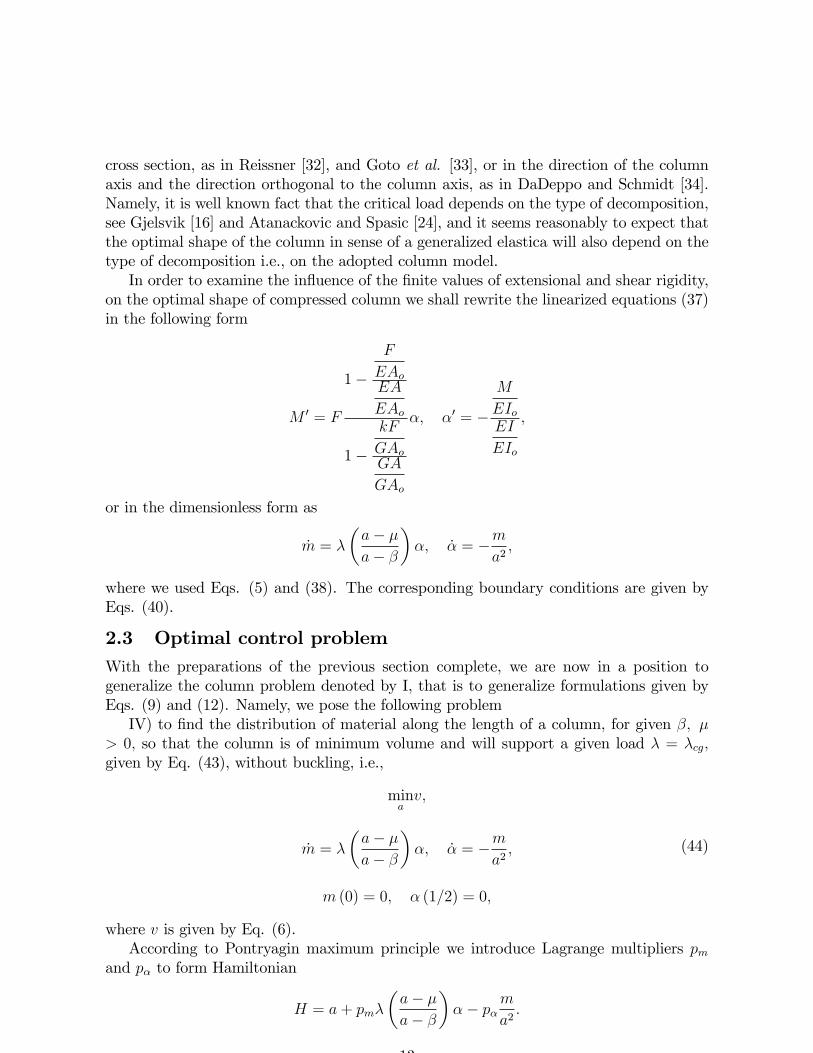
cross section, as in Reissner [32], and Goto et al. [33], or in the direction of the columnaxis and the direction orthogonal to the column axis, as in DaDeppo and Schmidt [34].Namely, it is well known fact that the critical load depends on the type of decomposition,see Gjelsvik [16] and Atanackovic and Spasic [24], and it seems reasonably to expect thatthe optimal shape of the column in sense of a generalized elastica will also depend on thetype of decomposition i.e., on the adopted column model.In order to examine the in�uence of the �nite values of extensional and shear rigidity,

on the optimal shape of compressed column we shall rewrite the linearized equations (37)in the following form

M 0 = F

1�

F

EAoEA

EAo

1�

kF

GAoGA

GAo

�; �0 = �

M

EIoEI

EIo

;

or in the dimensionless form as

_m = �

�a� �

a� �

��; _� = �m

a2;

where we used Eqs. (5) and (38). The corresponding boundary conditions are given byEqs. (40).

2.3 Optimal control problemWith the preparations of the previous section complete, we are now in a position togeneralize the column problem denoted by I, that is to generalize formulations given byEqs. (9) and (12). Namely, we pose the following problemIV) to �nd the distribution of material along the length of a column, for given �; �

> 0; so that the column is of minimum volume and will support a given load � = �cg;given by Eq. (43), without buckling, i.e.,

minav;

_m = �

�a� �

a� �

��; _� = �m

a2;

m (0) = 0; � (1=2) = 0;

(44)

where v is given by Eq. (6).According to Pontryagin maximum principle we introduce Lagrange multipliers pm

and p� to form Hamiltonian

H = a+ pm�

�a� �

a� �

��� p�

m

a2:

13

Then, the optimal distribution of the material a is determined from the relation

@H

@a= 0 = 1 +

2p�m

a3+��pm (�� �)

(a� �)2: (45)

The corresponding costate equations and natural boundary conditions are

_pm = �@H

@m=p�a2; _p� = �

@H

@�= �pm�

�a� �

a� �

�; (46)

pm (1=2) = 0; p� (0) = 0: (47)

We note that from Eqs. (45) and (47) it follows

a (0) = � +p� (� � �)� (0) pm (0); (48)

as a new result that generalizes the one given by Eq. (15). According to Eq. (48) theshape of the optimal column at its end depends on the load and material. In other wordsthe optimal shape becomes sensitive of the load and it seems it will �t for real columns.In order to get the optimal shape for several values of � and � we calculate Euler

buckling load �rst � = �cg and then we solve two point boundary value problem (44),(46) and (47) with a obtained as a solution of Eq. (45). At each step of integratingprocedure Eq. (45) is solved numerically by bisection method. All numerical integrationsfor shooting method were based on Bulirsch-Stoer integration procedure [23]. In Table1. we present minimum half volume vmin, the minimal and the maximal area of thecolumn cross section, that is, amin = a (0) and amax = a (1=2) : For comparison, in Table1 Clausen solution, that corresponds to zero values of � and �; and the critical value�c = �2 = 9:869, here obtained by numerical solution of the column problem. as a specialcase is also presented.

Table 1.

� � � vmin amax = a (1=2) amin = a (0)0.0 0.0 9.869 0.433 1.1547 00.0003 0.0001 9.868 0.433 1.1548 0.01870.003 0.001 9.850 0.434 1.1552 0.05980.03 0.01 9.670 0.440 1.1584 0.19590.3 0.1 7.676 0.476 1.1471 0.6693

The optimal shapes of the column that correspond to several values of column para-meters obtained by numerical integration of two point boundary value problem (44), (46)and (47), with a obtained as a solution of Eq. (45), are presented in Figure 5. As before,in Figure 5, we present optimal curve obtained as Ropt (t) =

paopt (t); which according

to Pearson formulation of the Lagrange problem, gives the column of greatest e¢ ciency.

14

Figure 5. Optimal shapes that generalize Clausen�s solution.

We note that �nite values of shear and extensional rigidity did change Clausen�s solu-tion as expected. We conclude by noting that, along the lines of Keller [3] or Atanackovic[35], the results presented here could be generalized by introducing imperfections in theshape and loading and by allowing di¤erent boundary conditions. An interesting type ofboundary conditions, applicable to optimal design of water tower is presented in Spasicand Glavardanov [36].

3 Optimal shape of the column against spatial buckling

In this section we wish to consider the buckling of a column subjected to a twisting coupleand compressive axial load. The ends of the column are assumed to be attached to thesupports by ideal spherical hinges and are free to rotate in any directions. As before onehinge is �xed whereas the other one is free to move along the axis z: We assume that thecolumn is loaded by a concentrated force F and a twisting couple K having the actionline along the z axis which coincide with the column axis in the unloaded state in whichthe column is straight and prismatic, see Figure 6.

Figure 6. Load con�guration and spatially buckled column.

Also, let us assume that during buckling the force and the couples K retain theirinitial directions. Although under such conditions the couple K is non conservative, seeTimoshenko and Gere [37], we intend to apply Euler method of stability analysis or themethod of adjacent equilibrium. In this case the de�ection curve C will not be a planecurve.

3.1 Equilibrium equations of a compressed and twisted columnAs before, the column under consideration is of circular cross section and will be repre-sented by the incompressible curve of centers C and circles attached to each point of that

15

curve. In what follows we introduce the line joining centroids of circular cross sectionsas a space curve C. We can represent that curve with respect to a reference frame Oxyzwith i; j and k as the corresponding unit vectors, �xed at the origin O; by means of avector

r =x (S) i+y (S) j+z (S)k;

where S is the Lagrange coordinate as usual. It is assumed that a unit vector orthogonalto the plane of the circle and the tangent to the column axis at each point of the curve C;coincide. These facts are interpreted as the absence of axial and shear deformations. Atthe centroid of any circle an orthogonal coordinate system Cx1y1z1 is constructed withcorresponding unit vectors i1; j1 and k1: The axis z1 is orthogonal to circle. In unloadedstate unit vectors i; j;k and i1; j1;k1 coincide, see Figure 7. Then to each circle we attachearea A(S) and Euler angles = (S) ; � = � (S) and ' = ' (S) ; recording orientation ofthe system Cx1y1z1 to the reference frame Oxyz: Namely, we introduce a circle of area A,and three spherical angles of Euler type as the parameters recording material orientationto that curve.Euler angles describe any possible orientation in terms of a rotation abut the y

axis, then a rotation � about the new x axis, and �nally, a rotation about new z axis of ':According to that sequence of rotations the following geometrical relations between unitvectors i1; j1 and k1 and unit vectors i; j and k hold, see Atanackovic [31],

i1 = (cos cos'+ sin sin � sin') i+cos# sin' j+ (cos sin � sin'� sin cos')k;

j1 = (sin sin � cos'� cos sin') i+cos � cos' j+(sin sin'+ cos sin � cos')k;(49)

k1 = sin cos �i� sin � j+cos cos �k:Also the change of unit vectors i1; j1 and k1 along the curve C is given by

i01 = !3 j1 � !2k1;

j01 = !1 k1 � !3i1; (50)

k01 = !2i1 � !1j1;

where (�)0 = d (�) =dS; and where

!1 = 0 cos � sin'+ �0 cos';

!2 = 0 cos � cos'� �0 sin'; (51)

!3 = � 0 sin � + '0:

The elastic deformation of the column can be described by the components of curvature!1; !2; and !3 that represents the twist around the axis z1. We note here that this typeof Euler angles, usually called Krilov or �ship� type, see Lurie38, is important becausethe small di¤erence in orientation of the systems Oxyz and Cx1y1z1 restricts the value ofeach of these angles. Also, the fact that this type allows the �rst two angles to be smalland the third one to be �nite will be useful latter.A typical element of the column with force and moment resultants acting on it is

shown in Figure 7.

16

Figure 7. Space curve coordinates and free body diagram of column element.

We assume that there are no static forces or moments distributed along the columnelement. The condition of force equilibrium applied to the column element yields thefollowing equation

dP

dS= 0: (52)

Similar, from consideration of the free body diagram of Figure 7, i.e., summing momentsabout a point S yields

dM

dS+dr

dS�P =0; (53)

wheredr

dS= x0i+ y0j+ z0k: (54)

According to the column model it is obvious that dr=dS and k1 coincide so the followinggeometrical relations hold

x0 = sin cos �; y0 = � sin �; z0 = cos cos �: (55)

Finally, assuming linear elastic behavior the connection between the geometrical quantitiesand the components of the resultant moment

M (S) =M1i1 +M2j1 +M3k1 (56)

could be given byM1 = EI!1; M2 = EI!2; M3 = GJ!3; (57)

where EI and GJ are bending and torsional rigidity respectively. These constitutiveequations form the ordinary approximate theory, a generalization of the classical Bernoulli-Euler plane elastica, and represent the classical Kirchho¤�s model of spatially buckledcolumn with no shear and axial deformations, see Eliseyev [39], and no torsion-warpingdeformation, see Simo and Vu-Quoc [40]. For a column of circular cross section theconnection between EI and GJ reads

GJ =EI

(1 + �); (58)

17

where � is the Poisson�s ratio. Also, as before EI could be expressed as EA2= (4�) :We state now the boundary conditions corresponding to the column shown in Figure

6. According to the usual sign convention we write

P (L) = �Fk; (59)

M (L) = Kk; (60)

and note that P(0) and M (0) equals P (L) and M (L) respectively. We also add thefollowing geometrical conditions

x (0) = 0; y (0) = 0; z (0) = 0; (61)

' (0) = 0; (62)

x (L) = 0; y (L) = 0: (63)

The equations (52), (53) could be interpreted in two di¤erent frames either Oxyz orCx1y1z1: In the �rst case we integrate Eq. (52) with boundary condition (59) and we get

P = P (S) = �Fk: (64)

Also, integrating Eq. (53) with boundary condition (60) gives

M = Fyi�Fxj+Kk; (65)

where we used Eqs. (64), (54) and (60). In the second case by use of Eqs. (50) we writeEqs. (52) and (53) in the following form

P 01 � P2!3 + P3!2 = 0;

P 02 � P3!1 + P1!3 = 0; (66)

P 03 � P1!2 + P2!1 = 0;

M 01 �M2!3 +M3!2 � P2 = 0;

M 02 �M3!1 +M1!3 + P1 = 0; (67)

M 03 �M1!2 +M2!1 = 0;

that corresponds to a physical space. Substituting Eqs. (57) into Eqs. (67) lead tothe well known theory known as Kirchho¤�s kinetic analogue, see Nikolai [1] or Love[18]. Namely, the equilibrium equations of a spatially buckled column and Lagrange�scoordinate S 2 [0; L] are interpreted as the equations of motion of a heavy rigid bodyturning about �xed point and time respectively. Note, that in optimization theory Eqs.(66) and (67) were �rst used by Keller [3] who considered the problem of optimal shapeagainst buckling of a naturally straight but twisted column subjected to a compressiveload. In his work Keller assumed that no twisting couple is applied. Referring againto Love [18] we note that Euler buckling load for a compressed and twisted column ofuniform cross section, determined by Greenhill in 1883, is given by�

K

2EIo

�2+

F

EIo=�2

L2: (68)

18

so the bifurcation analysis of the problem in this section will be omitted.Finally, the equilibrium equations of the compressed and twisted column could be

written in a visual space as well. Namely, we connect Eqs. (56) and (65) by use of Eqs.(49) and then substitute Eqs. (51) and (57). As a result, after some calculations, we getthe equilibrium equations of spatially buckled column in the following nonlinear form

x0 = sin cos �; y0 = � sin �;

z0 = cos cos �;

0 =

�Fy

EIsin +

K

EIcos

�tan � � Fx

EI; (69)

�0 =Fy

EIcos � K

EIsin ;

'0 =

�Fy

GJsin +

K

GJcos

�cos � +

�Fx

GJ+

�Fy

EIsin +

K

EIcos

�tan � � Fx

EI

�sin �:

The corresponding boundary conditions are given by Eqs. (61), (62) and (63).We note that if, as before, we treat only symmetric buckling mode, in which the

resultant moment achieve the maximum value at the middle of the column, that is forS = L=2; then instead of Eq. (63) we could use the following relations

y (L=2) = 0; (L=2) = 0: (70)

Namely, using Eq. (65) and the necessary condition

d jMjdS

=F (xx0 + yy0)pF 2 (x2 + y2) +K2

= 0;

together with Eqs. (55) we get Eqs. (70). Note that for the case K = 0; which impliesy = 0 and � = 0; we recover Eqs. (2).As we did in the introduction, we shall use the full nonlinear equations, given by Eqs.

(69), to examine the postbuckling behavior of the column of uniform cross section andthe same volume as the optimal one. For that purpose, we shall cast the problem intonon dimensional form. Namely, we de�ne

� =KL

EIo; � =

y

L; � =

z

L; (71)

and noteGJoEIo

=1

(1 + �):

Then we rewrite Eqs. (69) in the following form

_� = sin cos �; _� = � sin �;_� = cos cos �;

_ =1

a2[(�� sin + � cos ) tan � � ��] ; (72)

19

_� =1

a2(�� cos � � sin ) ;

_' =1

a2f(1 + �) (� cos + �� sin ) cos � + [��� + (�� sin + � cos ) tan �] sin �g ;

where we used Eqs. (5) as well. The corresponding boundary conditions read

� (0) = 0; � (0) = 0; � (0) = 0; ' (0) = 0; � (1=2) = 0; (1=2) = 0: (73)

The two point boundary problem (72), (73) admits a trivial solution in which the columnremains straight but twisted

� � 0; � � 0; � = t; � 0; � � 0; ' =(1 + �) �

a2t;

where the value of twisting angle ' is not necessary small, but is �nite.

3.2 Formulation of the problemIn order to determine the optimal shape, we shall linearize the nonlinear equilibriumequations. For the type of Euler angles we use here, the linearized equations are simplyobtained from Eqs. (72) as

_� = ; _� = ��;

_ =�� � ��

a2; _� =

�� � �

a2; (74)

_' =� (1 + �)

a2;

where � variable is omitted. The corresponding boundary conditions are

� (0) = 0; � (0) = 0; ' (0) = 0; � (1=2) = 0; (1=2) = 0: (75)

Also, from Eq. (68) that determines the critical load for a uniform column, transformedinto non dimensional form, we can express dimensionless force � = FL2=EIo in terms ofdimensionless twisting couple � = KL=EIo as

� = �2 � �2

4: (76)

Now we are ready to pose another problem that generalizes formulation given by Eqs.(9) and (12). Namely, we consider the problemV) to �nd the distribution of material along the length of a column, so that the column

is of minimum volume and will support a load for given � and � determined from (76),without buckling, i.e.,

minav;

_� = ; _� = ��; _ =�� � ��

a2; _� =

�� � �

a2; _' =

(1 + �) �

a2; (77)

� (0) = 0; � (0) = 0; ' (0) = 0; � (1=2) = 0; (1=2) = 0:

20

where:

(�) = d (�) =dt and where v is given by Eq. (6).Now we introduce Lagrange multipliers p�; p�; p ; p� and p' to form Hamiltonian

H = a+ p� � p�� + p �� � ��

a2+ p�

�� � �

a2+ p'

(1 + �) �

a2:

Then, according to Pontryagin�s maximum principle we �nd the optimal distribution ofthe material a as a solution of the following equation

@H

@a= 0 = 1� 2 [p (�� � ��) + p� (�� � � ) + p'� (1 + �)]

a3; (78)

that isaopt =

3

q2 [p (�� � ��) + p� (�� � � ) + p'� (1 + �)]: (79)

The corresponding costate equations for this generalization of the column problem are

_p� =�p a2

; _p� = ��p�a2

; _p = �p� +�p�a2; _p� = p� �

�p a2

; _p' = 0: (80)

Finally, the natural boundary conditions read

p� (1=2) = 0; ; p (0) = 0; p� (0) = 0; p� (1=2) = 0; (81)

andp' (1=2) = 0: (82)

We note that from (81) and (82) follow that a (0) = 0: Also that a (t) will be very smallin the neighborhood of t = 0. For small values of a any activity connected with numericalprocedure of solving two point boundary value problem given by Eqs. (77), (79), (80),(81), and (82) is rather complicated because of the sti¤ equation problem that appears.The situation will be even more complicated if we had chosen to generalize problem III,given by Eqs. (11) and (14), with the nonlinear di¤erential equations as a model. Wenote that some sti¤ equations can be handled by a change of variables, see Acton [41],but we shall avoid that problem here on the basis of physical considerations. Namely, ifwe propose the value of the twist angle at the middle of the column, say

' (1=2) = 'p; (83)

that is, if we use (83) instead of (82) then we expect the value p' = const:; to di¤er fromzero. Thus, the value aopt (0) given by

aopt (0) =3

q2p' (1 + �) �; (84)

will also di¤er from zero.The next problem to be solved is the value of 'p . Namely, for the uniform column

of volume v = v1 in trivial equilibrium con�guration, in which the column is straight buttwisted, the twist angle at the middle reads

'1=2 =(1 + �) �

2: (85)

21

In the formulation of the optimization problem we expect to get the volume of optimalcolumn, say vmin to be less then v1 so the value of the twisting angle that corresponds theuniform column of the same volume as optimal, say 's will be greater then '1=2: Thus, wepropose 'p to be greater then '1=2: As a result we expect the values 'p and 's to be close,and that the value of vmin to be in correlation with the di¤erence 'p � 's: Also, for thevery small values of the twisting couple � we expect the optimal shape of the compressedand twisted column to be very close to the Clausen�s solution presented in Figure 3.

3.3 Numerical resultsIn this section we present the results of the numerical integration of the linearized equilib-rium equations and necessary conditions for optimality given by Eqs. (77), (79), (80), (81),and (83). As before the shooting method is used. Initial guess (0) ; � (0) ; p� (0) ; p� (0)and p' (0) is improved by Newton method. All numerical experiments are done in thearea of small � and � near �c as suggested by Biezeno and Grammel [42]. Namely, thereal compressed and twisted columns are loaded near Euler buckling load �c = �2 andsmall value of twisting couple. In all the numerical calculations the value � = 0:3 is used.In Table 2. we present the minimum half volume vmin, the minimal and maximal area ofthe column cross section, that are amin = a (0) and amax = a (1=2) ; obtained for a fewvalues of � and � and for a few values of 'p. The area of the uniform column of the samesize as optimal as and the corresponding value of the twisting angle at trivial equilibriumcon�guration 's are also presented.

Table 2.

� � 'p vmin amax = a (1=2) amin = a (0) as 's

0.05 9.8680:0730:049

0:4360:446

1:1471:116

0:2660:531

0:8710:893

0:0430:041

0.25 9.8540:2440:179

0:4460:480

1:1161:042

0:5330:866

0:8930:960

0:2040:177

1.0 9.6200:8780:748

0:4540:472

1:0981:057

0:6410:811

0:9070:944

0:7900:728

The optimal shapes that correspond to the numerical solutions of the column arepresented in Figure 8. As in previous section instead of aopt (t) we present optimal curveobtained as Ropt (t) =

paopt (t); which according to Pearson formulation of the Lagrange

problem, gives the compressed and twisted column of greatest e¢ ciency.

22

Figure 8. Optimal columns against spatial buckling.

For comparison we note that the columns presented in Figure 8. could still remainstraight but the uniform columns made of the same amount of material, loaded withthe same � and � are very far away in the postcritical region. We shall examine thepostbuckling behavior of the column of uniform cross section as = 0:907; loaded with� = 9:62 and � = 1:0: For these values the nonlinear two point boundary value problem(72), (73) is solved numerically. In Figure 9. we present the projection of the column axisC on the Oxy plane.

Figure 9. Postbuckling behavior of compressed and twisted uniform column.

Along the lines of the remarks of the previous section we note that instead of Kirch-ho¤�s model of elastic rod we could use some other. Namely, we could analyze the e¤ectof shear and compressibility in spatial buckling problem. In doing so either Haringx�s,see Elyseyev [39] or Simo and Vu-Quoc [40], or Timoshenko type of decomposition, seeKingsbury [43], could be considered.Finally, another note that could be related to the problem of Lagrange is connected

with constrains on control variable. In application, optimal control problems where con-vexity assumption for the control domain is not needed are mathematically attractive aswell as technically signi�cant, see Nagahisa and Sakawa [44]. Roughly speaking, in theproblem of Lagrange we could propose the strongest column to be made of only a fewcircular cross sections of di¤erent size, i.e., in our notation it means to impose constraint

a 2 fa1; :::; alg;

for a few given real numbers a1; :::; al : This could reduce the column weight as well asthe expenses of column production. In practical terms the remarks above mean that thecolumn problem allows some more formulations and still remains open.

4 Closure

We have presented two possible generalizations of the well known problem of determiningthe optimum shape of a column for which the buckling load is largest among all columnsof given length and volume. First, the optimal shape of the column that can su¤er notonly �exure as in the classical elastica theory but also compression and shear is obtained.Our boundary value problem given by Eqs. (44) - (47) represents a considerable gener-alization of the column problem posed within the classical elastica theory. Consequently,the solution to our problem presented in Figure 5., generalizes Clausen�s solution thatcorresponds to the classical theory. In attacking our problem we have employed several

23

di¤erent, though equivalent formulations, of the governing equations in order to deal withdi¤erent questions that could be correlated with the optimal shape of a column againstbuckling. Second, by use of Kirchho¤�s kinetic analogue the distribution of material alongthe length of a compressed and twisted column hinged at either end is optimized so thatthe column is of minimum volume and will support a given load without spatial buck-ling. As before our boundary value problem given by Eqs. (77), (79), (80), (81) and (83)generalizes the classical column problem. Once again the solution to our problem, that isobtained by shooting method and presented in Figure 8., generalizes Clausen�s solution.Necessary conditions for both problems we treated here are derived using the maximumprinciple of Pontryagin. The principal novelty of the present results is that both solutions,that follow from two possible generalizations of the classical Bernoulli-Euler bending the-ory, lead to the optimum column with non-zero cross sectional area at its ends. A fewpossible generalizations of the column problem are also discussed.

Acknowledgments

This paper is largely based on the author�s Ph.D. thesis (Department of Mechanics, Uni-versity of Novi Sad, 1993), written under the direction of Professor Teodor Atanackovic.The author is grateful to Professor Atanackovic for shearing his insights into Theory ofRods. Also author would like to thank Professor Bozidar Vujanovic for introducing himto Optimization Theory.

References

[1] E. L. Nikolai, Lagrange�s problem of optimal shape of a column, Izv. Leningr. Po-litekh. Inst. 255, 8, 1907, (in Russian), reprinted inWorks on Mechanics, G.I.T.T.L.,Moskow, 1955.

[2] I. Tadjbakhsh and J. B. Keller, Strongest columns and isoperimetric inequalities,ASME J. Appl. Mech. 159, 29, 1962.

[3] J. B. Keller, The shape of the strongest column, Arch. Rational Mech. Anal. 275, 5,1960.

[4] N. S. Trahair and J. R. Booker, Optimum elastic columns, Int. J. Mech. Sci. 973,12, 1970.

[5] N. Olho¤ and S. Rasmussen, On single and bimodal optimum buckling loads ofclamped columns, Int. J. of Solids and Structures 605, 13, 1977.

[6] W. Prager and J. E. Taylor, Problems of optimal structural design, ASME J. Appl.Mech. 102, 34, 1968.

[7] G. I. N. Rozvany and Z. Mroz, Analytical methods in structural optimization, Appl.Mech. Reviews 1461, 30, 1977.

[8] G. N. Vanderplaats, Structural optimization - past, present, and future, AIAA Jour-nal 992, 20, 1982.

[9] N. Olho¤ and J. E. Taylor, On structural optimization, ASME J. Appl. Mech. 1139,50, 1983.

[10] D. C. Barnes, Buckling of columns and rearrangements of functions, Quart. Appl.Math. 169, 41, 1983.

[11] D. C. Barnes, The shape of the strongest column is arbitrarily close to the shape of

24

the weakest column, Quart. Appl. Math. 605, 46, 1988.[12] A. Seiranian, On a problem of Lagrange,(in Russian),Mekhanika Tverdogo Tela, 101,

19, 1984.[13] R. H. Plaut, L. W. Johnson and N. Olho¤, Bimodal optimization of compressed

columns on elastic foundations, ASME J. Appl. Mech. 130, 53, 1986.[14] S. J. Cox and M. L. Overton, On the optimal design of columns against buckling,

SIAM J. Math. Anal. 287, 23, 1992.[15] S. S. Antman and C. S. Kenney, Large buckled states of nonlinearly elastic rods

under torsion, trust, and gravity, Arch. Rational Mech. Anal. 289, 76, 1981.[16] A. Gjelsvik, Stability of built-up columns, ASCE J. Eng. Mech. 1331, 117, 1991.[17] D. F. Parker, An asymptotic analysis of large de�ections and rotations of elastic rods,

Int. J. Solids Structures 361, 15, 1979.[18] A. E. H. Love, A Treatise on the Mathematical Theory of Elasticity 4th ed., Dover,

New York, 1944.[19] C. D. Chung and N. Zung, On problems of optimal rods, (in Russian), Prikl. Mekhan.

95, 15, 1979.[20] A. S. Bratus and I. A. Zharov, On optimal design of elastic rods, (in Russian), Prikl.

Mekhan. 86, 26, 1990.[21] D. E. Kirk, Optimal Control Theory, Prentice Hall, Englewood Cli¤s, 1970.[22] V. M. Alekseev, V. M. Tihomirov and S. V. Fomin, Optimal Control, (in Russian),

Science, Moskow, 1979.[23] W. H. Press, B.P. Flannery, S. A. Teukolsky and W. T. Vetterling, Numerical Recipes

Cambridge Univ. Press., Cambridge, 1986.[24] T. M. Atanackovic and D. T. Spasic, A model for plane elastica with simple shear

deformation pattern, Acta Mechanica 241, 104, 1994.[25] J. D. Renton, Generalized beam theory applied to shear sti¤ness, Int. J. Solids Struc-

tures 1955, 27, 1991.[26] M. A. Krasnoselskii, A. I. Perov, A. I. Povolockii and P.P Zabreiko, Vector �elds on

plane, (in Russian), Fizmatigz., Moscow, 1963.[27] S. N. Chow and J. K. Hale, Methods of Bifurcation Theory, Springer, Berlin, 1982.[28] H. Troger and A. Steindl, Nonlinear Stability and Bifurcation Theory, Springer, Wien,

1991.[29] S. S. Antman and G. Rosenfeld, Global behavior of buckled states of nonlinearly

elastic rods, SIAM Review 513, 20, 1978.[30] V. Hutson and J. S. Pym, Aplications of Functional Analysis and Operator Theory,

Academic Press, London, 1980.[31] T. M. Atanackovic, Stability Theory of Elastic Rods, World Scienti�c, Singapore,

1997.[32] E. Reissner, On one-dimensional large-displacement �nite-strain beam theory, J.

Appl. Math. Phys. (ZAMP) 795, 23, 1972.[33] Y. Goto, T. Yoshimitsu and T. Obata, Elliptic integral solutions of plane elastica

with axial and shear deformations, Int. J. Solids Structures 375, 26 1990.[34] D. A. DaDeppo and R. Schmidt, Large de�ections of elastic arches and beams with

shear deformation, J. Industrial Math. Soc. 17, 22, 1972.[35] T. M. Atanackovic, Stability of a compressible elastic rod with imperfections, Acta

25

Mechanica 203, 76, 1989.[36] D. T. Spasic and B. V. Glavardanov, Stability of a rigid sphere supported by a thin

elastic column, Eur. J. Mech. A/Solids 337, 15, 1996.[37] S. P. Timoshenko and J. M. Gere, Theory of Elastic Stability, McGraw-Hill, NewYork,

1961.[38] A. I. Lurie, Analytical Mechanics, (in Russian), Gosudarst., Moskva, 1961.[39] V. V. Eliseyev, The non-linear dynamics of elastic rods, (in Russian), Prikl. Matem.

Mekhan. 493, 52, 1988.[40] J. C. Simo and L. Vu-Quoc, A geometrically exact rod model incorporating shear

and torsion-warping deformation, Int. J. Solids Structures 371, 27, 1991.[41] F. S. Acton, Numerical Methods that Work, Harper and Row, New York, 1970.[42] C. B. Biezeno and R. Grammel, Technische Dynamic, 2nd. Ed., Springer, Berlin,

1953.[43] H. B. Kingsbury, A reexamination of the equations of motion of a curved and twisted

rod, ASME Design Engineering Division Conference and Exibit on Mechanical Vi-bration and Noise, Cincinnati, Ohio, 1985.

[44] Y. Nagahisa and Y. Sakawa, A new computational algorithm for solving optimalcontrol problems, Numer. Func. Anal. Optimiz. 1019, 11, 1990.

26

27