Optimal Control Theory Applied to Ship Maneuvering in

Restricted Waters

Brian S. Thomas and Paul D. Sclavounos

Department of Mechanical EngineeringMassachusetts Institute of Technology

Abstract

Ship drivers have long understood that powerful interaction forces exist when ships operatein close proximity to rigid boundaries or other vessels. Controlling the effects of these forceshas been traditionally handled by experienced helmsmen. The purpose of this study is to applymodern optimal control theory to such maneuvering scenarios in order to show that helmsmenmay some day be replaced by modern controllers. The maneuvering equations of motion are castin a linear state space framework, permitting the design of a linear quadratic (LQ) controller.The hydrodynamic effects are modelled using potential flow theory in order to simulate theinteraction forces and test the performance of the controller. This study demonstrates that thelinear quadratic regulator effectively controls ship motions due to the presence of a boundary orother vessel over a broad range of speeds and separation distances. Viscous effects are modelledby equivalent linearization and when compared to the effective damping introduced by thecontroller, are shown to be insignificant.

1 Introduction

The problem of controlling ships during their passages at sea has a history as old as human maritimeendeavors. The past century saw great advances in control theory. The age old marine problemswere among the first applications to benefit from these innovations. Notably marine autopilots werea primary test bed as feedback control systems were beginning to be formalized in a mathematicalsetting during the early 1900s. In today’s age of ever faster paced, higher efficiency operations, astrong focus on optimal routing and collision avoidance has emerged and the current control theoryliterature has numerous examples of the sophisticated work going on in this area. Research howeverappears to be less extensive on the effect of inter-vessel interaction forces and their use in the designof robust controllers. This is the subject of the present study.

1.1 The Hydrodynamic Problem

The interaction forces that develop between ships and banks in restricted waters have been under-stood on a practical level by mariners for centuries. Masters of large vessels take pains to keepprudent distances between vessels in order to moderate these forces.

In contrast to the wealth of practical knowledge of these phenomena and how best to controlthem, quantitative approaches are still relatively scarce. Model tests and full scale analyses havebeen conducted on a limited basis, and Principles of Naval Architecture [3], treats the subjectin some detail. More recently model tests have been reported on by Vantorre et al [8] for avariety of overtaking scenarios by ships of differing geometries. This work was primarily intended

1

for improving the accuracy of training simulators, however its application to the control problemcould be significant. Analytically, the most general work on this subject was undertaken by Tuckand Newman in 1974 [7]. Using slender body theory they propose a set of equations to evaluatethe hydrodynamic forces and moments between two slender bodies on parallel courses but witharbitrary speed, separation, and stagger. This model although only in moderate agreement withempirical results, can be useful in formulating and simulating control problems involving ship-shipinteractions.

1.2 The Control Problem

The ship maneuvering problem contains strongly coupled dynamics of the ship sway and yawmodes of motion. This coupling requires a multiple-input multiple-output (MIMO) approach tothe control problem. Modern state-space methods provide such a method. These state spacemethods minimize some cost, typically the deviation from a desired state and control usage, whilesubject to the constraints of the dynamics of the system. The popular linear quadratic (LQ) familyof controllers, take their name from the linearity of their state equation and the quadratic form oftheir cost function. One particular advantage of the LQ optimal control framework used here isthat the existence of a solution to the problem guarantees both optimality and stable control. Therobustness properties of LQ controllers are favorable enough to make them popular in a variety ofapplications, notably aircraft control.

This paper will address the specific maneuvering problem of a ship travelling next to a bank or itsimage. It will be shown that this problem generates a sway force and yaw moment in general, whichmake the system unstable. Ships typically control their motions by altering speed and rudder angle.For the bank suction problem it will be shown with an appropriate potential flow model that themagnitudes of the interaction forces are dependent on forward speed. Completely eliminating theeffect of the bank through speed change means stopping completely which is clearly not reasonable.Alternatively, applying a rudder angle generates both a sway force and yaw moment. For a shipproceeding parallel to a wall, a heuristic argument can be made that steady motion with constantseparation requires that the force and moment generated by a constant rudder must exactly balancethe interaction force and moment. This is not possible in the general case and so an LQ controllerdesign has been developed. The benefit of the using optimal control theory in this case is thatthe system’s dynamical properties are central to the controller design process. The controller’s‘knowledge’ of this dynamics allows it to find an equilibrium between control, hydrodynamic andinteraction forces. This equilibrium is demonstrated with a numerical simulation. In addition therelative importance of viscous forces has been addressed. Equivalent linearization for small sway andyaw motions allows viscous damping terms to be applied to the controlled system. The simulationdemonstrates that the viscous damping terms are much smaller than the damping introduced bythe controller and are thus negligible.

2 The Hydrodynamic Model

2.1 Overview

The goal of this hydrodynamic model is to determine the steady and unsteady hydrodynamicforces and moments exerted on a vessel due to the presence of another vessel or a vertical wall.The method of images is used to simulate the case where a ship is travelling parallel to a verticalboundary.

2

XY

Z

Figure 1: SWAN Domain Mesh (Asymmetric Body)

In the present study the 3D Rankine panel method SWAN (Ship Wave ANalysis) developed atMIT’s Laboratory for Ship and Platform Flows was used to evaluate the appropriate hydrodynamicquantities. More details on SWAN are presented in [5]

2.2 The Mathematical Model

The 3D potential flow problem is commonly expressed as a boundary value problem for the velocitypotential φ. In the present analysis the free surface is considered rigid. This approximation leadsto the classic “double body” flow.

The steady pressure distribution and resulting suction sway force and yaw moment follow fromBernoulli’s equation in terms of the steady double-flow potential φ1 arising from the ship forwardmotion:

p = −12ρ (∇φ1 · ∇φ1) + ρUφ1x (1)

#»

F =∫∫

SB

p #»ndS (2)

# »

M =∫∫

SB

p ( #»x × #»n) dS (3)

The added mass tensor follows from the classical expression

mij = ρ

∫∫

SB

φinjdS (4)

where φi is the unit double-body potential due to the i-th mode of motion of the vessel next to avertical wall and nj , j = 1, ..., 6 are the unit vectors on the ship boundary pointing out of the fluiddomain.

3

0.1 0.15 0.2 0.25 0.3 0.35 0.4 0.45 0.50

0.02

0.04

0.06

0.08

0.1

0.12

0.14

0.16

0.18

d/L

Attr

actio

n F

orce

Coe

ffici

ent

F2/(

0.5

ρ U

2 B T

)

0.1 0.15 0.2 0.25 0.3 0.35 0.4 0.45 0.5−1

0

1

2

3

4

5

6

7x 10

−3

d/L

Yaw

Mom

ent C

oeffi

cien

tM

6/(0.

5 ρ

U2 L

B T

)

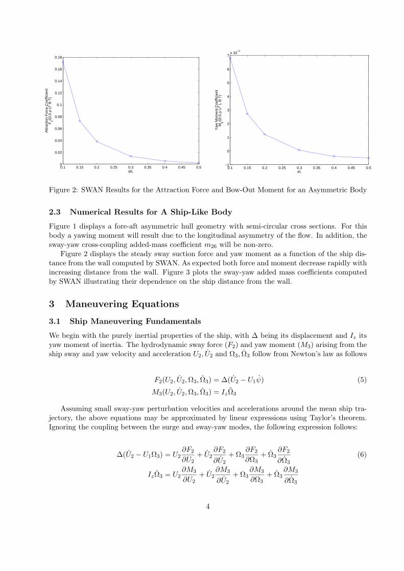
Figure 2: SWAN Results for the Attraction Force and Bow-Out Moment for an Asymmetric Body

2.3 Numerical Results for A Ship-Like Body

Figure 1 displays a fore-aft asymmetric hull geometry with semi-circular cross sections. For thisbody a yawing moment will result due to the longitudinal asymmetry of the flow. In addition, thesway-yaw cross-coupling added-mass coefficient m26 will be non-zero.

Figure 2 displays the steady sway suction force and yaw moment as a function of the ship dis-tance from the wall computed by SWAN. As expected both force and moment decrease rapidly withincreasing distance from the wall. Figure 3 plots the sway-yaw added mass coefficients computedby SWAN illustrating their dependence on the ship distance from the wall.

3 Maneuvering Equations

3.1 Ship Maneuvering Fundamentals

We begin with the purely inertial properties of the ship, with ∆ being its displacement and Iz itsyaw moment of inertia. The hydrodynamic sway force (F2) and yaw moment (M3) arising from theship sway and yaw velocity and acceleration U2, U2 and Ω3, Ω3 follow from Newton’s law as follows

F2(U2, U2, Ω3, Ω3) = ∆(U2 − U1ψ) (5)

M3(U2, U2, Ω3, Ω3) = IzΩ3

Assuming small sway-yaw perturbation velocities and accelerations around the mean ship tra-jectory, the above equations may be approximated by linear expressions using Taylor’s theorem.Ignoring the coupling between the surge and sway-yaw modes, the following expression follows:

∆(U2 − U1Ω3) = U2∂F2

∂U2+ U2

∂F2

∂U2

+ Ω3∂F2

∂Ω3+ Ω3

∂F2

∂Ω3

(6)

IzΩ3 = U2∂M3

∂U2+ U2

∂M3

∂U2

+ Ω3∂M3

∂Ω3+ Ω3

∂M3

∂Ω3

4

0.1 0.15 0.2 0.25 0.3 0.35 0.4 0.45 0.50.85

0.9

0.95

1

1.05

1.1

1.15

1.2

d/L

A22

/(ρ

V)

0.1 0.15 0.2 0.25 0.3 0.35 0.4 0.45 0.5−0.05

−0.048

−0.046

−0.044

−0.042

−0.04

−0.038

−0.036

−0.034

−0.032

−0.03

d/L

A26

/(ρ

V L

)

0.1 0.15 0.2 0.25 0.3 0.35 0.4 0.45 0.50.245

0.25

0.255

0.26

0.265

0.27

0.275

0.28

0.285

0.29

0.295

d/L

A66

/(ρ

V L

B)

Figure 3: SWAN Results for the Added Mass and Moments for an Asymmetric Body

Figure 4: Coordinate System

5

Assuming that a small rudder angle δR is applied, the linear sway and yaw force and momentgenerated may be included. Now the equations for the sway and yaw perturbation displacementsare governed by the matrix equation

[− ∂F2

∂U2+ ∆ − ∂F2

∂Ω3

−∂M3

∂U2−∂M3

∂Ω3+ Iz

] [U2

Ω3

]=

[∂F2∂U2

( ∂F2∂Ω3

−∆U1)∂M3∂U2

∂M3∂Ω3

][U2

Ω3

]+

[∂F3∂δR∂M3∂δR

][δR] (7)

In the present context, small deviations of the ship from its mean course are assumed. Therefore,the linear form of the equations 7 is acceptable for our purposes.

3.2 Hydrodynamic Derivatives

In order to estimate the hydrodynamic derivatives present in equation 7 we turn to classic potentialflow theory. In the equations for the force and moment on a moving body in an infinite and inviscidfluid and irrotational flow are presented by Newman [4]:

Fj = −Uimji − εjklUiΩkmli

Mj = −Uimj+3,i − εjklUiΩkml+3,i − εjklUiUkmli (8)

In these equations the index i goes from 1,. . .,6, while j, k, l can only take values 1,2,3. Ui is thevelocity in the three rectilinear modes of motion, Ωk are the three angular velocities, and εjkl isthe alternating tensor. In our case, only the sway (U2), yaw (U6,Ω3) and surge (U1) modes areof interest, as all other velocities are assumed to be zero. In addition, the perturbation surgeforce (F1) is assumed negligible compared to the propeller thrust required to maintain the steadyforward velocity of the ship. Based on these assumptions we may now determine the sway and yawperturbation hydrodynamic force and moment F2 and M3:

F2 = −U2m22 − Ω3m26 − U1Ω3m11

M3 = −U2m62 − Ω3m66 + U1U2(m11 −m22)− Ω3U1m26 (9)

If the ship forward velocity U1 in the x-direction is assumed constant, these two equations providedesired expressions for the hydrodynamic derivatives required in the maneuvering equations. Itfollows that

∂F2

∂U2= 0

∂M3

∂U2= U1(m11 −m22)

∂F2

∂Ω3= −U1m11

∂M3

∂Ω3= −U1m26

∂F2

∂U2

= −m22∂M3

∂U2

= −m62

∂F2

∂Ω3

= −m26∂M3

∂Ω3

= −m66 (10)

With the derivatives so defined, equation 7 may be rewritten in terms of the known added masscoefficients.

[m22 + ∆ m26

m62 m66 + Iz

] [U2

Ω3

]=

[0 −U1(m11 + ∆)

−U1(m22 −m11) −U1m26

] [U2

Ω3

]+

[FR

MR

][δR]

(11)

6

4 Control

4.1 Optimal Control Problem

Stengel [6] covers the derivation of the Linear Quadratic Regulator (LQR) and that derivation willnot be repeated here. However, the basic problem is to minimize some quadratic cost functionJ constrained by the dynamics of the system. The system dynamics are contained in the stateequation:

x = Ax + Bu + D (12)

In this equation x is the state vector, u is the control vector, and D is a matrix containing dis-turbances to the system. A is the plant matrix obtained from the derivation of the equations ofmotion. B is an input matrix, stating the linear law that states the effect of the control parametersu upon the state vector x.

The quadratic cost function takes the form:

J =12

∫ T

0

(xTQx + uTRu

)dt (13)

Here Q is a positive semi-definite matrix containing the costs associated with deviations from thedesired mean value of the state. R is a positive definite matrix containing the costs associated withthe control usage.

With the problem defined as above, the linear quadratic regulator now states that u(t) is theoptimal control trajectory provided that:

u(t) = −R−1BPx(t) (14)

Where P is the solution to the algebraic matrix Riccati equation.

0 = PA + ATP−PBR−1BTP + Q (15)

Conventionally, the control law is stated in a compact matrix form as follows:

u(t) = −Kx(t) (16)

whereR−1BP = K (17)

K is known as the gain matrix, and is constant for constant time-invariant A and B matrices.Therefore, K may be calculated a priori and used throughout the system’s operation.

4.2 The State Equation for the Steady Case

Now the equations of motion from the previous section may be rewritten for the steady case whereU1 is considered to be a constant. The unsteady case where the forward speed is allowed to varyslowly in time and used as a control will be treated later. For compactness we introduce thefollowing definitions:

mij =[

∆ + m22 M26 + m26

M26 + m26 Iz + m66

](18)

bij =[ −U1m22(xT ) U1(xT m22(xT )−∆)−U1(m22 + xT m22(xT )) U1(M26 + m26 − x2

T m22(xT ))

](19)

FR =

[12ρU2

1 S ∂CL∂δR

12ρU2

1 S ∂CL∂δR

xT

](20)

7

The state equation follows in the form:

U2

Ω3

ψy

=

m−1ij ·bij

00

00

0 1 0 01 0 U1 0

U2

Ω3

ψy

+

[m−1

ij ·FR

][δR] (21)

where ψ is the ship yaw angular displacement and y its sway displacement from their zero meanvalues.

4.3 Forward Speed as a Control

The control problem is now extended to the more realistic scenario where speed is also allowedto vary. For large vessels, speed changes occur very slowly due to their large inertia. Howeversmall changes in speed may have significant effects on the forces and moments and shouldn’tbe neglected. The attraction force and moment generated by the presence of another vessel orboundary are dependent on both separation distance and forward speed. These forces and momentsare expressed in the form:

F2 =12Cs(d)ρBTU2

M3 =12Cm(d)ρBTLU2 (22)

Here L, B, and T are the length, beam and draft of the vessel, respectively. Now if U is consideredto be the sum of the initial forward velocity and a small perturbation (U1 + δu) then the equationsbecome:

F2 =12Cs(d)ρBT (U2

1 + 2U1δu + δ2u)

M3 =12Cm(d)ρBTL(U2

1 + 2U1δu + δ2u) (23)

The final term in this expression is of second order and can be neglected, however, the second termdirectly shows the effect of the perturbation velocity (δu) on the the suction force and moment.Keeping only leading order terms in the perturbation:

F2 = Cs(d)ρBTU1δu

M3 = Cm(d)ρBTLU1δu (24)

These equations contain the effect of the forward speed variation on the side force and moment ofinterest.

Looking now at the effect of the perturbation velocity on the rudder forces and moments, wesee that the same analysis may be applied.

FR =12ρS

∂CL

∂δRδR(U2

1 + 2U1δu + δ2u)

MR =12ρSxT

∂CL

∂δRδR(U2

1 + 2U1δu + δ2u) (25)

Since both δR and δu are small, there exist no first order terms containing δu and so to leadingorder, small speed changes will not affect the performance of the rudder.

8

With all of the above taken into account, the state equation may be stated in its complete form:

x = Ax + Bu + D (26)

Where,

A =

m−1ij ·bij

00

00

0 1 0 01 0 U1 0

B = m−1

ij

[12ρU2

1 S ∂CL∂δR

Cs(d)ρBTU112ρU2

1 S ∂CL∂δR

xT Cm(d)ρBTLU1

](27)

with mij and bij as defined in equations 18 and 19. The state and control vectors respectively are:

x =

U2

Ω3

ψy

u =

[δR

δu

](28)

This set of state equations does not contain the body’s forward speed, U1, as a state variable. Inorder to remove this state variable we have made certain assumptions. First it is assumed thatsurge is not coupled to sway and yaw. Second it is also assumed that because the body is slender,(B/L ≈ 0.15), the surge added mass m11 is small compared to the ship mass. Finally, the mainpropulsive force is significantly greater than external hydrodynamic effects in surge.

4.4 Equivalent Linear Damping

Frequently viscous drag is approximated by a quadratic expression that is modelled by Morison’sequation. In order to incorporate the quadratic force expressions into the linear model, drag must belinearized. It is here assumed that the ship sway and yaw motions may be expressed as oscillationsabout the ship mean path,

ξ2 = |Ξ2| cos(ωt + ϕ)ξ6 = |Ξ6| cos(ωt + ϕ) (29)

The goal is to develop an equivalent linear damping mechanism B22V isc ξ2 which dissipates the sameamount of energy per cycle as the quadratic damping obtained from the application of Morison’sequation. The resulting expressions for the linear sway and yaw damping coefficients are:

B22V isc =4ρCDAP

3πω|Ξ2| (30)

and similarly for yaw:

B66V isc =4ρCDMP

3πω|Ξ6| (31)

The definition of the frequency ω, drag coefficient CD, sway projected area AP and yaw projectedarea second moment MP are discussed below.

9

Table 1: Symmetric Body CharacteristicsLength(L) 100mBeam(B) 15mDraft(T) 7.5m

Cb 0.52Rudder Area (S) 18.75 m2

∂CL∂δR

4.71

5 Control System Simulation

5.1 Overview

In order to test the viability of the control system under consideration, a numerical simulation ofthe maneuvering problem was carried out. Namely, a vessel was modelled travelling next to a solidboundary in infinite depth. Utilizing the linear equations of motion derived previously and thehydrodynamic properties calculated by SWAN, the motion of the body was calculated for a varietyof scenarios.

The simulation program, written with MATLAB, uses the state equation and the hydrodynamicproperties generated by the hydrodynamic model to calculate the gain matrix K. Through thecontrol law the controller specifies the control vector u in terms of the contemporaneous value ofthe state vector x. The force model sums the control, attraction and disturbance forces and appliesthem to the right hand side of the maneuvering equations of motion.

5.2 Rudder Modelling

While rudder sizes and shapes vary greatly with the purpose of the vessel, a rudder planform area(S) equal to 2.5% of the area of a rectangle formed by the vessel’s length and draft is a good baselineestimate. If the rudder is modelled as a flat plate with a maximum span equal to the draft, inthree dimensions the lift coefficient as a function of rudder angle (δR) may be approximated by theclassical expression:

CL =2πAe

Ae + 2δR (32)

Here Ae is the effective aspect ratio. Because the free surface has been modelled as a rigid plane,it acts as a plane of symmetry. Thus the aspect ratio of the rudder is effectively doubled to twiceits conventional definition. The fundamental dimensions and rudder properties for the symmetricbody are listed in Table 1

5.3 Inherent System Instability

Prior to applying the control, it is important to understand the system behavior in the absence ofcontrols. Without the application of any controls the state equation simply becomes:

x = Ax (33)

If the solution to this equation may be cast in the form:

x(t) = c1eλt (34)

the differential equation becomes,λ c1e

λt = Ac1eλt (35)

10

xi max

U2 = 0.1 m/sΩ3 = 0.57 /sψ = 5.7

y = 0.1 myi = 0.5 m·s

ui maxδR = 2.5

δu = 0.25 m/s

Table 2: Maximum State and Control Values

where by cancelling the eλt term it can be seen that λ are the eigenvalues of A. From equation34 it can be seen that in order for the solution to decay from an initial displacement to its initialvalue x0 the real parts of all eigenvalues λ must be negative.

For both symmetric and asymmetric vessel geometries, there exists an eigenvalue of A whichhas a positive real part. As a result, any perturbation will lead to unbounded deviation from theinitial state.

5.4 The Cost Matrices Q and R

Prior to using the simulation, suitable values for the state cost and control cost matrices must bedetermined. Bryson [1] gives a general rule for the diagonal cost matrices. If each state and controlvariable has a maximum desired value of xi max and ui max respectively, then:

Qii =1

ximax2Rii =

1uimax2

(36)

Typical values for ximax and uimax are displayed in Table 2.

5.5 Integral Feedback

Initial simulations indicate that the model achieves a stable steady state result with a constantrudder angle and speed offsetting the constant attraction force and moment from the wall. When itreaches a steady state however the vessel has an offset from its initial separation distance. In orderto minimize this steady state drift error an additional state variable is added. Stengel [6] discussesthe addition of an integral feedback state variable in order to overcome steady state errors.

If y is the cross track error in the state equation as displayed in equation 26, we can add anadditional state variable.

yi =∫ t

0y(τ)dτ yi(t) = y(t) (37)

11

0 20 40 60 80 100 120 140 160 180 200

−0.2

0

0.2

0.4

0.6

Time(s)

Cro

ss T

rack

Err

or (

m)

0 20 40 60 80 100 120 140 160 180 200−6

−4

−2

0

2

Time (s)

Rud

der

Ang

le (

°)

0 20 40 60 80 100 120 140 160 180 200−1

−0.5

0

Time(s)

Spe

ed C

hang

e (m

/s)

w/o Integral Feedbackw/ Integral Feedback

Figure 5: Integral Feedback Control History Comparison (Fn = 0.16, d = 15 m)

With the addition of this state variable the state equation now becomes:

U2

Ω3

ψyyi

=

m−1ij ·bij

00

00

00

0 1 0 0 01 0 U1 0 00 0 0 1 0

U2

Ω3

ψyyi

+

m−1ij ·

[12

∂CL∂δR

ρSU21 Cs(d)ρBTU1

12

∂CL∂δR

ρSU21 xT Cm(d)ρBTLU1

]

0 00 00 0

[δR

δu

](38)

Implementing this new state equation eliminates the steady state error as may be seen in figure 5.

5.6 Significance of Viscous Effects

Having developed linear expressions for viscous damping in both sway and yaw, the relative impor-tance of these effects may be determined. B22V isc and B66V isc may be added to the state equation.This yields a new controller which has an A matrix and gain affected by the presence of theequivalent linear viscous terms.

x = [A−BK]Viscx (39)

If the controlled system is thought of as a classical mechanical oscillator, the controller providesboth a damping effect when acting on the U2 and Ω3 state variables, as well as restoring effect whenacting on the integral state variables y and ψ. The damping and restoring effects, with or withoutviscous effects, may be seen though the classical analysis of such systems. The general solution tothe homogeneous equation 39 is:

x(t) = c1eλ1t + c2e

λ2t (40)

12

0 1 2 3 4 5 6 7 8 9 100

0.5

1

1.5

2

2.5

3

3.5

|Ξ2|/Beam (%)

Dam

ping

Incr

ease

% D

ecre

ase

in M

ax λ

(R

eal P

art)

Ξ6 = 0°, Fn = 0.16

0 0.5 1 1.5 2 2.5 3 3.5 4 4.5 50

0.005

0.01

0.015

0.02

0.025

0.03

0.035

0.04

0.045

|Ξ6| (°)

Dam

ping

Incr

ease

% D

ecre

ase

in M

ax λ

(R

eal P

art)

Ξ2 = 0, Fn = 0.16

Figure 6: Damping Increase Dependence on Assumed Sway and Yaw Amplitude

In general the eigenvalues (λ) may be complex of the form (a + bi) so that the general solutionbecomes

x(t) = d1eat cos bt + d2e

at cos bt (41)

x is considered to be a vector of oscillations about the nominal state, with frequency b and amplitudeeat. The eigenvalue of [A−BK]Visc with the greatest real part, a, will control the damping orstability of the entire system. The viscous terms must always take energy out of the system, soviscous effects increase damping and decrease a. In order to determine the significance of thisincrease, the real parts of the largest (least negative) eigenvalue of [A−BK] and [A−BK]Visc arecompared.

Quantifying the damping terms in equations 30 and 31 requires a suitable selection of |Ξ2|, |Ξ6|, ωand CD. A CD of 1 was selected for bluff body cross sections. For ω, the imaginary parts of theeigenvalues of [A−BK] provide a reasonable value of 0.15 rad/sec (see figure). The magnitudes of|Ξ2|, |Ξ6| and forward speed are varied. Figure 6 shows that as the sway and yaw amplitudes areallowed to increase, there is a linear increase in the damping of the controlled system. The figurealso indicates that the sway amplitude has a far greater effect on damping than yaw.

Since forward speed plays a vital role in the effectiveness of the controls, the relative effectof viscous damping at various speeds was also calculated. Figure 7 shows the increase in thecontrolled system damping when viscous effects are added over a range of speeds for two differentsway amplitudes. The lower the sway amplitude (represented by the solid line) the more realisticthe controller performance. Even when less realistic sway amplitudes are considered at a low speed,the viscous effects only contribute a 5% increase in the total system damping. At more relevantamplitudes and speeds, viscous effects contribute only 1% to the total damping. These resultsdemonstrate that control forces dominate the system performance, while viscous effects are quitesmall by comparison.

5.7 Controlled System Stability

Simulations indicate stable behavior over a range of separation distances and speeds. Speeds rangedfrom Froude numbers of 0.064 to 0.255. Centerline to wall separation distances ranged from 10 to

13

0.06 0.08 0.1 0.12 0.14 0.16 0.18 0.2 0.22 0.24 0.260.5

1

1.5

2

2.5

3

3.5

4

4.5

5

5.5

Fn

% D

ecre

ase

in M

ax λ

(R

eal P

art)

Ξ2 = 0.375 m, Ξ

6 = 5°

Ξ2 = 1.5 m, Ξ

6 = 5°

Figure 7: Damping-Increase Dependence on Forward Speed

60 meters. With the controller on, the stability of the system may be determined by examining theeigenvalues of [A−BK]. For the entire range of scenarios tested, the real parts of the eigenvaluesfor the controlled state equation, [A−BK], are all negative, indicating stable behavior of thecontrolled system. Figure 8 is a plot of the eigenvalues and associated control history for thecontrolled system operating at two different speeds. As these figures show, changes to the initialsimulation parameters of speed and separation alter the position of eigenvalues on the complexplane and thus the response of the controller. Reducing the initial forward speed and increasingthe separation distance both bring the eigenvalues closer to the imaginary axis, reducing stability,and increasing the time required to reach steady state.

5.7.1 The Controller’s Use of Speed

In every case the control system chooses to reduce speed in reaching steady state. Some limitationsof the controller simulation and design become clear when looking at the speed changes called forby the controller. For the minimum separation (d/L = 0.1), the speed reduction is greater than10% at all initial speeds and should not be considered small.

5.7.2 The Controller’s Use of Rudder

For every scenario simulated the controller achieves a steady state rudder angle. In general, thissteady state rudder angle is negative. A rudder angle which should turn the vessel towards the wallis perhaps counter intuitive at first.

Looking back to equation 8, there is a term in the moment equation that when taken alonebecomes:

M3 = U1U2(m11 −m22) (42)

14

−0.2 −0.15 −0.1 −0.05 0 0.05 0.1 0.15 0.2−0.2

−0.15

−0.1

−0.05

0

0.05

0.1

0.15

0.2

Re

Im

d/L = 0.15, Fn = 0.16d/L = 0.15, Fn = 0.10

0 20 40 60 80 100 120 140 160 180 200

−0.1

0

0.1

0.2

0.3

Time (s)

Cro

ss T

rack

Err

or (

m)

0 20 40 60 80 100 120 140 160 180 200−6

−4

−2

0

2

Time (s)

Rud

der

Ang

le (

°)

0 20 40 60 80 100 120 140 160 180 200−1.5

−1

−0.5

0

Time (s)

Spe

ed C

hang

e (m

/s)

d/L = 0.15, Fn = 0.16d/L = 0.15, Fn = 0.10

Figure 8: [A−BK] Eigenvalues and Associated Control History

Considering the heading angle ψ the equation becomes:

M3 = −U2sin(ψ)cos(ψ)(m11 −m22) (43)

For long slender bodies (m11 − m22) < 0 so the moment is positive in sign and destabilizing ingeneral. This effect is known as the“Munk Moment”.

In order to overcome the suction due to the wall on the starboard side, the control system turnsthe ship to port a small amount, known generally as a crab angle. With the small but steadynegative heading angle, a negative Munk moment is present and so the controller must counteractthis with a negative rudder angle. Here again, as separation grows large the required rudder anglediminishes. An analogous study involving the seakeeping, motion control and stability of high-speedhydrofoil vessels using a similar LQ controller is presented in [2].

6 Conclusion

Applying modern optimal control theory it has been shown that the hydrodynamic interactioneffects of a ship with a vertical wall or similar vessel on a parallel course may be mitigated. Thecontroller strikes a careful balance between interaction, control and maneuvering forces in order toreach a stable steady state. Viscous forces have been estimated through equivalent linearization.When the damping effects of these viscous terms are compared to the damping effects induced bythe controller, it is clear that the physical viscous effects are insignificant and may be neglected.

References

[1] A.E. Bryson and Y. Ho. Applied Optimal Control. Hemisphere Publishing, 1975.

[2] I.I. Chatzakis and P. D. Sclavounos. Active control of a high-speed hydrofoil vessel using state-space methods. Journal of Ship Research, 2005.

[3] E.V. Lewis, editor. Principles of Naval Architecture, volume III. Society of Naval Architectsand Marine Engineers, 2nd edition, 1989.

15

[4] J.N. Newman. Marine Hydrodynamics. The MIT Press, 1977.

[5] P.D. Sclavounos, S. Purvin, U. Talha, and S. Kim. Simulation based resistance and seakeepingperformance of high-speed monohull and multihull vessels equipped with motion control liftingappendages. In Keynote Lecture, FAST 2003 Conference, Ischia Italy., 2003.

[6] R.F. Stengel. Optimal Control and Estimation. Dover, 1994.

[7] E.O. Tuck and J.N. Newman. Hydrodynamic interactions between ships. In Proceedings for the10th Symposium on Naval Hydrodynamics, pages 35–70, 1974.

[8] M. Vantorre, Erik Laforce, and Ellada Verzhbitskaya. Model test based formulations of ship-shipinteractions forces for simulation purposes. In International Marine Simulator Forum, 2001.

16