optimal control of discrete-time hybrid automata under ...€¦ · optimal control of discrete-time...

Nonlinear Analysis 65 (2006) 1188–1210www.elsevier.com/locate/na

Optimal control of discrete-time hybrid automata undersafety and liveness constraints

Carla Seatzua,∗, Dmitry Gromovb, Jorg Raischb,c, Daniele Coronaa,Alessandro Giuaa

a Dip. di Ing. Elettrica ed Elettronica, Universita di Cagliari, Italyb Lehrstuhl fur Systemtheorie technischer Prozesse, Otto-von-Guericke-Universitat Magdeburg, Germanyc Systems and Control Theory Group, Max-Planck-Institut fur Dynamik komplexer technischer Systeme,

Magdeburg, Germany

Abstract

In this contribution we address an optimal control problem for a class of discrete-time hybrid automataunder safety and liveness constraints. The solution is based on a hierarchical decomposition of the problem,where the low-level controller enforces safety and liveness constraints while the high-level controllerexploits the remaining degrees of freedom for performance optimization. Lower-level control is based ona discrete abstraction of the continuous dynamics. The action of low-level control can be interpreted asrestricting invariants in the hybrid automaton representing the plant model. A state feedback solution forthe high-level control is provided, based on the off-line construction of an appropriate partition of the statespace.c© 2005 Elsevier Ltd. All rights reserved.

Keywords: Hybrid automata; Switched systems; Safety constraints; Liveness constraints

1. Introduction

Hybrid automata are dynamic systems that consist of both continuous dynamics (modeledby a set of differential or difference equations) and a switching scheme (modeled by invariants

∗ Corresponding address: Universita di Cagliari, Dept. of Electrical and Electronic Engineering, Piazza d’Armi, 09123Cagliari, Italy. Tel.: +39 70 675 5853; fax: +39 70 675 5900.

E-mail addresses: [email protected] (C. Seatzu), [email protected] (D. Gromov),[email protected] (J. Raisch), [email protected] (D. Corona), [email protected](A. Giua).

0362-546X/$ - see front matter c© 2005 Elsevier Ltd. All rights reserved.doi:10.1016/j.na.2005.12.024

http://www.elsevier.com/locate/na

mailto:[email protected]





http://dx.doi.org/10.1016/j.na.2005.12.024

C. Seatzu et al. / Nonlinear Analysis 65 (2006) 1188–1210 1189

and guards). Hybrid automata (and other modeling paradigms for hybrid systems) have beenwidely investigated because of their importance in many application areas. Often, the controlobjective for such systems is to minimize a cost function while respecting safety and livenessconstraints. There are a number of abstraction-based control synthesis approaches that addresssafety and liveness issues while largely ignoring performance optimization aspects [8,19,16,11].On the other hand, very interesting papers on the optimal control of hybrid systems have beenpresented, but the proposed approaches are often not able to handle “hard” safety constraints.Among these we mention [4,10,14,18,21,20,22,24,25].

In this paper we provide a method for synthesizing a state feedback control strategy whichminimizes a given cost function under certain safety and liveness constraints.

More precisely, the contribution of this paper is threefold and can be summarized in thefollowing items.

• Firstly, we investigate how the action of an approximation based discrete supervisor can beinterpreted as restricting invariants of the hybrid automaton plant model. This has been brieflydescribed in the conference papers [7,9]. In this contribution, we provide a much more detailedexposition.

• Secondly, we extend our previous results on the optimal control and stabilization of switchedsystems [6] and hybrid automata [4,7,5] where a technique was presented for solving aninfinite time horizon optimal control problem for a hybrid automaton whose continuousdynamics are affine, when a quadratic performance index is considered.

Here we generalize our previous results in two ways:

(a) we take into account the existence of forbidden regions assuming that the invariant set invi

of a location i ∈ L may be a proper subset of Rn , i.e., invi � Rn ;

(b) we assume that an infinite number of switches is allowed.

We show that a state feedback solution based on the off-line construction of an appropriateswitching region, that we call a switching table, can be computed. Each point of the tableuniquely determines the corresponding optimal mode.

• The third contribution consists in combining the above approaches in order to deal with theoptimal control of discrete-time hybrid automata under safety and liveness constraints. Moreprecisely, the problem is divided in two hierarchical levels. The low-level controller enforcessafety and liveness constraints, and can be interpreted as restricting invariants in the hybridautomaton representing the plant model. The high-level control uses the remaining degrees offreedom to perform optimization.

The paper is structured as follows. In Section 2, we recall some basic facts on hybrid automata,introduce the plant model and formalize the specifications. In Section 3, the safety and livenessrequirements are addressed using �-complete abstraction of the continuous plant dynamics. InSection 4, the remaining degrees of freedom are used to minimize a quadratic cost function. InSection 5, a numerical example is provided.

Finally, a remark regarding terminology. As time, i.e. the domain of signals, is discretethroughout this paper, the words “continuous” and “discrete” will always refer to the rangeof signals: continuous signals live in dense subsets of some Euclidean space, whereas discretesignals live in discrete, and for the purpose of this paper, finite sets; continuous (respectivelydiscrete) systems are characterized by continuous (respectively discrete) signals.

1190 C. Seatzu et al. / Nonlinear Analysis 65 (2006) 1188–1210

Fig. 1. A graph describing a hybrid automaton.

2. Plant model and specifications

In this section we first define the class of Hybrid Automata (HA) on which we focus attention.Then we formally describe the safety specifications and the optimal control problem.

2.1. Hybrid automata

Like a continuous-time hybrid automaton [12,1], a discrete-time hybrid automaton HAconsists of a “classic” automaton extended with a continuous state. The latter, denoted byx(k) ∈ Rn , evolves in discrete time k ∈ N0 with arbitrary dynamics. The hybrid automatonconsidered here is a structure HA = (L, X, f, inv, E) which, in complete analogy to, e.g. [2], isdefined as follows:

• L = {1, . . . , α} is a finite set of locations.• X ⊆ Rn is a continuous state space.• fi : X → X is a function that associates with each location i ∈ L a discrete-time difference

equation of the form

x(k + 1) = fi (x(k)). (1)

• inv : L → 2X is a function that associates with each location i ∈ L an invariant invi ⊆ X .• E ⊂ L ×2X × L is the set of edges. An edge ei, j = (i, gi j , j) ∈ E is an arc between locations

i and j with associated guard region gi j . The set of edges can be interpreted as the discretepart of the overall hybrid automaton as shown in Fig. 1. This is a directed graph with verticescorresponding to the locations (state-graph). The state-graph is assumed to be connected.

The pair (l(k), x(k)) represents the hybrid state at time k, where l(k) is the discrete locationl(k) ∈ L and x(k) ∈ Rn is the continuous state.

Starting from initial state ξ0 = (i, x0) ∈ L × X , x0 ∈ invi , the continuous state x may evolveaccording to the corresponding discrete-time transition function fi , i.e., x(k + 1) = fi (x(k)),until it is about to leave the invariant invi , i.e. fi (x(k)) �∈ invi , k ∈ N0. This enforces a switchto another location j satisfying the guard constraint x(k) ∈ gi j and x(k) ∈ inv j ; the futureevolution of the continuous state is now determined by the transition function f j , providedthat the condition f j (x(k)) ∈ inv j holds. If several potential “follow-up” locations satisfy theconstraint, this degree of freedom can be exploited by an appropriate discrete control scheme.Thus, the sequence l(k) of discrete locations can be interpreted as a constrained control input.Note that the hybrid automaton may also switch to a “new” location j before being forced toleave its “old” location i , if the corresponding guard constraint and “new” invariant are satisfied.


It may also happen that for some state (l(k), x(k)) the system evolution cannot be extended tothe interval [k + 1,∞). This situation is referred as blocking. The notion of liveness, in turn,corresponds to the fact that the system evolution can always be extended to infinity. In thispaper the liveness property of interest for the system considered is assumed to be equivalent tononblocking. This is described formally in Section 2.3. Obviously, the initial hybrid automatondoes not necessarily possess the liveness property. A first goal of low-level control is to assurethis property along with safety specifications.

2.2. The plant model

In this paper we assume that the uncontrolled plant is modeled as a specific discrete-timehybrid automaton satisfying the following assumptions:

A1. The difference equation (1) is linear and time-invariant, i.e.

x(k + 1) = Ai x(k) ∀i ∈ L, k ∈ N0. (2)

A2. invi = X ∀i ∈ L.A3. Transitions between any two locations i, j ∈ L are allowed.A4. gi j = X ∀i, j ∈ L.

Note that assumption A3 does not reduce the generality of the approach, since possiblerestrictions on discrete transitions can be considered as specifications—this will be illustrated inSection 3.2.1. Under the assumptions A1–A4, the uncontrolled plant is a switched linear systemwith a free input signal l : N0 → L.

It will turn out in Section 3.3 that adding low-level control to the plant model will addnontrivial invariants to the plant automaton. This may be interpreted as adding state spaceconstraints that force the plant dynamics to respect safety and liveness constraints.

2.3. Safety and liveness specification

To formalize safety specifications, the continuous plant state space X is partitioned via afunction qy : X → Yd , where Yd is a finite set of symbols. To express dynamic safety constraints,certain sequences of input/output symbols are declared illegal or, in other words, the evolution ofthe hybrid automaton needs to be restricted such that only legal (L, Yd )-sequences are generated.It is assumed that this set of sequences can be realized by a finite automaton P . The procedureof “building” such an automaton is described in detail in Section 3.2.1.

The liveness requirement implies that ∀i ∈ L, ∀k ∈ N0, the following must hold: x(k) ∈invi , fi (x(k)) �∈ invi ⇒ ∃e = (i, gi j , j), x(k) ∈ gi j and x(k + 1) = f j (x(k)) ∈ inv j . Note thatthe liveness condition guarantees the existence of an evolution (i(k), x(k)), k ∈ N0, from everyinitial hybrid state (i, x0).

2.4. Optimal control problem

Subject to plant model, safety and liveness constraints, we aim at minimizing the cost function

J =∞∑

k=0

x(k)′Ql(k)x(k), (3)

where, for each k ∈ N0 and l(k) ∈ L, Ql(k) is a positive semidefinite real matrix.


This problem will now be approached using a two-level control hierarchy. Safety and livenessrequirements are being taken care of by the low-level control. This is described in Section 3. Theremaining degrees of freedom are used to minimize the cost function (3). This is described inSection 4.

3. The low-level task

In a first step, the hybrid plant automaton is approximated by a finite state machine employingthe �-complete approximation approach [16,11]. Subsequently, Ramadge and Wonham’ssupervisory control theory (e.g. [17]) is used to synthesize a least restrictive supervisor.Note that, in general, controller synthesis and approximation refinement are iterated until anontrivial supervisor guaranteeing liveness and safety for the approximation can be computedor computational resources are exhausted. In the former case, attaching the resulting supervisorto the hybrid plant model amounts to introducing restricted invariants. The resulting hybridautomaton represents the plant under low-level control and can be guaranteed to respect bothsafety and liveness constraints.

3.1. Ordered set of discrete abstractions

The low-level control deals with a continuous system (2) with discrete external signals.l : N0 → L is the discrete control input and yd : N0 → Yd the discrete measurement signalgenerated by

yd(k) = qy(x(k)). (4)

The set of output symbols, Yd , is assumed to be finite: Yd = {y(1)d , . . . , y(β)

d }, and qy : X → Yd

is the output map. Without loss of generality, the latter is supposed to be surjective (onto). Theoutput map partitions the state space into a set of disjoint subsets Y (i) ⊂ X, i = 1, . . . , β, i.e.

β⋃i=1

Y (i) = X,

Y (i) ∩ Y ( j ) = ∅ ∀i �= j.

To implement supervisory control theory, the hybrid plant model is approximated by a purelydiscrete one. This is done using the method of �-complete approximation [16,11], which isdescribed in the following paragraphs.

Denote the external behavior of the hybrid plant model by Bplant, i.e. Bplant ⊆ (L × Yd )N0 isthe set of all pairs of (discrete-valued) input/output signals w = (l, yd) that (2) and (4) admit. Ingeneral, a time-invariant system with behavior B is called �-complete if

w ∈ B ⇔ σ kw |[0,�] � w |[k,k+�] ∈ B |[0,�] ∀k ∈ N0,

where σ is the unit shift operator and w |[0,�] denotes the restriction of the signal w to thedomain [0, �] [23]. For �-complete systems we can decide whether a signal belongs to the systembehavior by looking at intervals of length �. Clearly, an �-complete system can be representedby a difference equation in its external variables with lag �. Hence, for an �-complete system afinite range for its external signals can be realized by a finite state machine. However, the hybridplant model Bplant is, except for in trivial cases, not �-complete. For such systems, the notion


of strongest �-complete approximation has been introduced in [11]: a time-invariant dynamicalsystem with behavior B� is called the strongest �-complete approximation for Bplant if

(i) B� ⊇ Bplant,

(ii) B� is �-complete,(iii) B� ⊆ B� for any other �-complete B� ⊇ Bplant,

i.e. if it is the “smallest” �-complete behavior containing Bplant. Obviously, B� ⊇ B�+1 ∀� ∈ N,and hence the proposed approximation procedure may generate an ordered set of abstractions.Clearly, w ∈ B� ⇔ w |[0,�] ∈ Bplant |[0,�] . For w |[0,�] = (l0, . . . , l�, y(i0)

d , . . . , y(i�)d ) this is

equivalent to

fl�−1

(· · · fl1

(fl0(q

−1y (y(i0)

d )) ∩ (q−1y (y(i1)

d )))

· · · (q−1y (y

(i�−1)

d )))

∩ q−1y (y(i�)

d )

� X (w |[0,�]) �= ∅. (5)

Note that for a given string w |[0,�], X (w |[0,�]) represents the set of possible values for thecontinuous state variable x(�) if the system has responded to the input string l(0) = l0, . . . , l(�−1) = l�−1 with the output yd(0) = y(i0)

d , . . . , yd (�) = y(i�)d . Note also that (5) does not depend

on l(�). For linear and affine systems evolving in discrete time N0, (5) can be checked exactly,as all sets involved are polyhedra.

As both input and output signal evolve on finite sets L and Yd , B� can be realized by a(nondeterministic) finite automaton. In [16,11], a particularly intuitive realization is suggested,where the approximation state variable stores information on past values of l and yd . Moreprecisely, the automaton state set can be defined as

Xd :=�−1⋃j=0

Xd j , � ≥ 1,

where Xd0 = Yd , and Xd j is the set of all strings (l0, . . . , l j−1, y(i0)d , . . . , y

(i j )

d ) such that

(l0, . . . , l j , y(i0)d , . . . , y

(i j )

d ) ∈ B |[0, j ] .

The temporal evolution of the automaton can be illustrated as follows:From initial state xd(0) ∈ Xd0, it evolves through states

xd( j) ∈ Xd j , 1 ≤ j ≤ � − 1

while

xd( j) ∈ Xd�−1, j ≥ � − 1.

Hence, until time �−1, the approximation automaton state is a complete record of the system’spast and present, while from then onwards, it contains only information on the “recent” past andpresent.

As the states x (i)d ∈ Xd of the approximation realization are strings of input and output

symbols, we can associate x (i)d with a set of continuous states, X (x (i)

d ), in completely the sameway as in (5).

Note that we can associate y(ik )d as the unique output for each discrete state xd(k) =

(lk− j , . . . , lk−1, y(ik− j )

d , . . . , y(ik )d ) ∈ Xd , j < �. Thus, the output is just the last symbol in the


Fig. 2. Moore-automaton (left) and an equivalent automaton without outputs (right). Note that y(ik )

d = μ(x(i j )

d ) ∈ Yd is

the output symbol associated with the discrete state x(i)d .

symbolic description of the state. It is then a straightforward exercise to provide a transitionfunction δ : Xd × L → 2Xd such that the resulting (nondeterministic) Moore-automatonM� = (Xd , L, Yd , δ, μ, Xd0) with state set Xd , input set L, output set Yd , output functionμ : Xd → Yd , and initial state set Xd0 is a realization of B�. Note that the state of M� isinstantly deducible from observed variables [15].

To recover the framework of supervisory control theory (e.g. [17]) as closely as possible, wefinally convert M� into an equivalent automaton without outputs, G� = (Xd ,Σ , δ, Xd0), whereΣ = L∪Yd , L represents the set of controllable events and Yd represents the set of uncontrollableevents.

Technically, this procedure is carried out according to the following scheme (for anillustration, see Fig. 2):

• Each state x ( j )d ∈ Xd is split into two states: x ( j )

d and x ( j )d . Thus, the new state set is formed

as Xd = Xd⋃

Xd . Initial states are replaced by their complements, Xd0 = Xd0 .• The new transition function δ is defined as a union of two transition functions with

nonintersecting domains:

δ(x (i)d , σ ( j )) =

⎧⎪⎨⎪⎩

�x (i)d , x (i)

d ∈ Xd , σ ( j ) = μ(x (i)d ) ∈ Yd ,

δ(x (i)d , σ ( j )), x (i)

d ∈ Xd , σ ( j ) ∈ L,

undefined, otherwise,

where � denotes an operation of taking the complementary state, i.e. �x (i)d � x (i)

d and viceversa. Note that the first event always belongs to the set Yd , and the following evolutionconsists of sequences where events from L and Yd alternate.

Note that since the function μ is scalar-valued, the set of feasible events for each state x ∈ Xd

contains only one element. Thus, any two states x and �x form a fixed pair, where the states Xd

are in some sense fictitious and play an auxiliary role.

3.2. Specifications and supervisor design

3.2.1. Formal specificationsIn the following, we consider specifications which consist of the independent specifications

for the input and the output.


Fig. 3. Transformation of state-graph to a finite automaton.

The specification on outputs expresses both static constraints (through restricting the set ofallowed outputs Y ∗

d ⊂ Yd ) and dynamic constraints. Dynamic constraints are usually represented

as a set of forbidden strings, “the symbol y( j )d follows immediately upon the symbol y(i)

d ”, or

“the symbol y(i)d appears three times consecutively without any other symbol in between”. The

set of all allowed strings is then realized as a finite automaton PY = (SY , Yd , δY , sY 0).The specifications for inputs, in turn, reflect structural restrictions on the allowed sequence

of input symbols. They can be extracted from the state-graph in Fig. 1 and realized by a finiteautomaton PL = (SL , L, δL , sL0) according to the algorithm shown in Fig. 3.

The last stage is the composition of input and output specifications to obtain the overallspecification P . Note that to be compatible with the approximation automaton G�, the overallspecification has to have a special transition structure, namely, it must generate only sequencesof events that consist of alternating symbols y ∈ Yd and l ∈ L, where the first symbol mustbelong to the set Yd (see Fig. 2 (right)). Thus, the resulting specification automaton is obtainedas an “ordered” product of PL and PY :

P = PY ∨ PL = (PY ‖PL) × Ω = (S, Yd ∪ L, δ, s0), (6)

where the automaton Ω is given by ({0, 1}, Yd ∪ L, ω, {0}),

ω(x, σ ) =⎧⎨⎩

1, x = 0, σ ∈ Yd ,

0, x = 1, σ ∈ L,

undefined, otherwise.

To characterize the resulting specification automata, we need the notion of current-stateobservability (cf. [3,13]):

Definition 3.1. A finite state machine A = (Q,Σ , φ) is said to be current-state observable ifthere exists a nonnegative integer K such that for every i ≥ K , for any (unknown) initial stateq(0), and for any admissible sequence of events σ(0) . . . σ (i − 1) the state q(i) can be uniquelydetermined. The parameter K is referred to as the index of observability.

In the following, we assume that the automata PL and PY are current-state observable withindices of observability K PL and K PY , respectively.

The notion of current-state observability can be extended to the overall specificationautomaton. Its index of observability K P is given by

K P ={

2K PY − 1, K PY > K PL ,

2K PL , K PY ≤ K PL .(7)


Furthermore, to stay within the time-invariant framework we have to restrict ourselves tospecifications that can be realized by strongly current-state observable automata:

Definition 3.2. A finite state machine A = (Q,Σ , φ) is said to be strongly current-stateobservable if it is current-state observable with observability index K and if for each state q ∈ Qthere exists another state q ′ ∈ Q such that the state q can be reached from q ′ by a sequence ofK events, i.e. ∀q ∈ Q ∃q ′ ∈ Q, s.t. q = φ(q ′, s), s ∈ Σ∗, |s| = K , where Σ∗ is the Kleeneclosure of Σ and φ the extension of the automaton transition function to strings in Σ∗.

Note that each state of such an automaton can be deduced from the string consisting of thepast K events, independently from the initial state.

3.2.2. Supervisor design

Given an approximating automaton G� and a deterministic specification automaton (6) withobservability index K P , supervisory control theory checks whether there exists a nonblockingsupervisor and, if the answer is affirmative, provides a least restrictive supervisor SUP via“trimming” of the product of G� and P . Hence the state set of the supervisor, XSUP, is a subsetof Xd × S.

The functioning of the resulting supervisor is very simple. At time k it “receives” ameasurement symbol which triggers a state transition. In its new state x ( j )

sup, it enables a subset

Γ (x ( j )sup) ⊆ L and waits for the next feedback from the plant. As shown in [11], the supervisor

will enforce the specifications not only for the approximation, but also for the underlying hybridplant model.

In the following, we will be interested in the special case of quasi-static specifications. Toexplain this notion, let papp : XSUP → X denote the projection of XSUP ⊆ Xd × S onto its firstcomponent. If papp is injective, i.e. if

papp(x1) = papp(x2) ⇒ x1 = x2, (8)

and, moreover, the specification is strongly current-state observable, then the specificationautomaton is called quasi-static with respect to the approximation automaton Gl .

Proposition 3.3. P is quasi-static with respect to G� if

2� − 1 ≥ K P . (9)

Proof (Sketch). Let x1 and x2 be two states of the supervisor SUP with papp(x1), papp(x2) ∈ Xd .There are two cases:

(1) papp(x1), papp(x2) ∈ Xd j , 1 ≤ j < � − 1. Each element from Xd j stores a record ofthe complete past and present of yd and l. Since the specification automaton is assumed tobe deterministic, this record unambiguously determines the current state of the specificationautomaton. Thus, (8) holds.

(2) papp(x1), papp(x2) ∈ Xd�−1 . In this case an element from Xd�−1 contains information only on“recent” past values of yd and l. Precisely speaking, it contains information about the last �

output symbols and the last � − 1 control symbols. Thus, the complete record has length of2� − 1 symbols, which is sufficient to unambiguously determine the current state of P .


3.3. Plant model under low-level control

For the case of quasi-static specifications, each supervisor state x (i)sup corresponds exactly to a

state x (i)d = papp(x (i)

sup) of the approximating automaton, which, in turn, can be associated with a

set X (x (i)d ) = X (papp(x (i)

sup)).For k ≥ � − 1, attaching the discrete supervisor to the plant model is therefore equivalent to

restricting the invariants for each location l j ∈ L according to

invl j =⋃

i, s.t.l j ∈Γ (x(i)sup)

papp(x(i)sup)∈Xd�−1

X (papp(x (i)sup))

⋃fi (X (papp(x (i)

sup))). (10)

Note that for the initial time segment, i.e. k < � − 1, (10) is more restrictive than the discretesupervisor computed in Section 3.2.

Hence the action of supervisory control is to restrict the invariants from inv j = X to inv j

given by (10) and, accordingly, to restrict the guards from gi j = X to gi j = invi ∩ inv j whereinvi and inv j are computed according to (10).

The union of all invariants invl j , j = 1, . . . , α, forms the refined state set that contains onlysafe points, i.e. points for which there exists at least one sequence of control symbols such thatthe resulting behavior satisfies the specifications.

The resulting hybrid automaton represents the plant model under low-level control (for k ≥ �).As control system synthesis has been based on an �-complete approximation, it is guaranteed thatthe resulting hybrid automaton satisfies safety and liveness requirements. The remaining degreesof freedom in choosing l(k) can be used in a high-level controller addressing performance issues.

4. The high-level task

The high-level task requires the solution of an optimal control problem of the form (3).The aim of this section is that of showing in detail that a state feedback solution of (3)

can be obtained by computing off-line appropriate partitions of the state space, that we callswitching regions, extending to the case at hand previous results on the optimal control ofswitched systems [20], based on dynamic programming arguments. In particular, we presentthe following three main results.

• Firstly, we recall how one can extend the results of [20] to the case of HA with invariantsin order to compute an optimal state feedback control law for the problem (3) when a finitenumber of switches N is allowed.

• Then, we show how the proposed approach can be easily extended to the case of an infinitenumber of allowed switches.

• Finally, we show how to deal with the case of hybrid systems whose dynamics are all unstable.

For sake of simplicity we will deal with completely connected automata. These results canbe easily extended to the case of generic automata using the same arguments as in [4], wherecontinuous-time HA were taken into account.


4.1. The optimal control problem with a finite number of switches

Let us now consider an optimal control problem of the form:⎧⎪⎪⎪⎪⎪⎪⎪⎨⎪⎪⎪⎪⎪⎪⎪⎩

V ∗N (i0, x0) � min

I,K

{F(I,K) �

∞∑k=0

x(k)′Qi(k)x(k)

}

s.t. x(k + 1) = Ai(k)x(k)

i(k) = ir ∈ L, for kr ≤ k < kr+1, r = 0, 1, . . . , Nx(k) = invi(k), for k = 0, 1, . . . ,+∞0 = k0 ≤ k1 ≤ · · · ≤ kN < kN+1 = +∞

(11)

where Qi are positive semidefinite matrices, (i0, x0) is the initial state of the system, andN < +∞ is the maximum number of allowed switches, that is given a priori.

In this optimization problem there are two types of decision variables:

• I � {i1, . . . , iN } is a finite sequence of modes;• K � {k1, . . . , kN } is a finite sequence of switching time indices.

Problem (11) is clearly well posed provided that the following hypotheses are verified.

Assumption 4.1. The invariant sets invi , i ∈ L, guarantee the liveness of the HA.

Note that Assumption 4.1 is generally not easy to verify. Nevertheless, in the case at hand,its satisfaction is guaranteed a priori by the low-level task, namely by the procedure used toconstruct the invariant sets.

Moreover, to ensure a finite optimal cost for any x0 ∈ Rn and any i0 ∈ L we assume thefollowing:

Assumption 4.2. There exists at least one mode i ∈ L such that Ai is strictly Hurwitz andinvi = Rn .

Note that this condition is sufficient but usually not necessary to get a finite optimal cost.In [20] it was shown that under the assumption that invi = Rn for all i ∈ L, the optimal

control law for the optimization problem (11) takes the form of a state feedback, i.e., it is onlynecessary to look at the current system state in order to determine whether a switch from lineardynamics Air−1 to Air should occur.

For a given mode i ∈ L when r switches are still available, it is possible to construct a tableCi

r that partitions the state space Rn into α regions R j , j = 1, . . . , α = |L|. Whenever iN−k = iwe use table Ci

r to determine whether a switch should occur: as soon as the continuous state xreaches a point in the region R j for a certain j ∈ L \ {i} we will switch to mode iN−k+1 = j ;no switch will occur if the continuous system’s state x belongs to Ri .

In [20] it was constructively shown how the tables Cir can be computed off-line using a

dynamic programming argument: first the tables Ci1 (i ∈ L) for the last switch are determined,

then, by induction, the tables Cir can be computed once the tables Ci

r−1 are known.

Remark 4.3. In order to provide a graphical representation of Cir we associate a different color

with each dynamics A j , j ∈ L. The region R j of Cir is represented according to the defined color

mapping.


Note that when invi = Rn for all i ∈ L, the regions R j are homogeneous, namely if x ∈ R j

then λx ∈ R j for all λ ∈ R. This implies that they can be computed by simply discretizing theunitary semisphere. Clearly, this is no longer valid when invi � Rn for some i ∈ L, as in thecase of interest here where a discretization of all state space of interest is necessary.

To show how the procedure of [20] can be extended to the case we are considering here, lety ∈ Rn be a generic vector, and let D be an appropriate set of points in the portion of the statespace of interest, that define the state space discretization grid considered. Moreover, given adiscrete state i ∈ L and a continuous state y ∈ Rn , we define the set

succ(y) = { j ∈ L | y ∈ inv j }which denotes the indices associated with the locations whose invariant set includes y.

The procedure for computing the switching regions is based on dynamic programming. Letus denote as Tr (i, y) the optimal remaining cost when the current continuous state is y, thecurrent dynamics is Ai and r switches are still available. Thus, when r = 0, i.e., when no moreswitches may occur, T0(i, y) = y ′Zi y if Ai is Hurwitz and the system trajectory starting in yand evolving with dynamics Ai until the origin is reached always keeps within invi . The matrixZi is the solution of the discrete Lyapunov equation A′

i Zi + Zi Ai = −Qi . In all the other cases,T0(i, y) = +∞.

The optimal remaining cost Tr (i, y) for r = 1, . . . , N is computed recursively starting fromr = 1 towards increasing values of r . More precisely, we first choose a finite time horizon kmaxthat is large enough to approximate the infinite time horizon. Then, for any r = 1, . . . , N , anyy ∈ D and any i ∈ L, we compute the value of the cost to infinity when the initial state is (i, y),r switches are still available, the generic dynamics Ai is used for the first k times of sampling,then the system switches to dynamics A j . This cost, that we denote as T (i, y, j, k, r), is thesum of the cost due to the evolution with dynamics Ai for k times of sampling, plus the optimalremaining cost from the new state ( j, Ak

i y) reached after the switch when r − 1 switches are stillavailable, i.e.,

T (i, y, j, k, r) = y ′(

k∑h=0

(Ahi )′Qi (Ah

i )

)y + Tr−1( j, Ak

i y). (12)

The previous equation expresses the dynamic programming argument used to efficiently computethe optimal switching law. When r switches are still available, we consider a nominal trajectorystarting from a discretization grid point y and evaluate its cost assuming that we remain in thecurrent dynamic i for a time k; the cost remaining after the switch is evaluated on the basis of thetable previously constructed for the r − 1 switch. Note that for fixed values of i , y, j and r weonly need to find the optimal value of k with a one-dimensional search.

Note that only those evolutions that do not violate the invariant constraints should be takeninto account. This means that if z = Ak

i y is the generic continuous state reached from y evolvingwith dynamics Ai for k steps, an evolution with dynamics A j , j ∈ L, should be considered ifand only if j ∈ succ(z).

Finally, we define the switching tables as mappings Cir : D → L, and the generic region R j

as

R j = {y ∈ D | Cik(y) = j}.

The procedure for computing the switching regions is briefly summarized in the followingalgorithm.


Algorithm 4.4 (Tables Construction). Input:

Ai ∈ Rn×n , Qi ∈ Rn×n, invi ⊆ Rn (i ∈ L), N, kmax,D.

Output:

Cir , r = 0, 1, . . . , N, i ∈ L .

Notation:

Qi (k) =k∑

h=0

(Ahi )′Qi (Ah

i ), Zi = limk→∞ Qi (k).

(1) Initialization: r = 0 remaining switchesfor i = 1 : α

for all y ∈ DCost assignment:

T0(i, y) =

⎧⎪⎪⎨⎪⎪⎩

y ′Zi y if Ai is Hurwitz and the system trajectory startingin y and evolving with dynamics Ai until the originis reached, always keeps within invi

+∞ otherwise

end (y)end (i )

(2) for r = 1 : Nfor i = 1 : α

for all y ∈ DComputation of the remaining cost:let k = 0, Δ = ∅while k ≤ kmax

z = Aki y

if z /∈ invi

for all j ∈ succ(z)T (i, y, j, k, r) = y ′Qi (k)y + Tr−1( j, k),Δ = Δ ∪ {( j, k)}

end ( j )k = kmax + 1

elsefor all j ∈ succ(z) \ {i}

T (i, y, j, k, r) = y ′Qi (k)y + Tr−1( j, k),Δ = Δ ∪ {( j, k)}

end ( j )k = k + 1

end ifend whileif i ∈ succ(y) and Ai is Hurwitz

T (i, y, i, kmax, r) = y ′Zi y,Δ = Δ ∪ {(i, kmax)}

end if


Cost assignment: Tr (i, y) = min( j,k)∈Δ

T (i, y, j, k, r)

Color assignment: ( j∗, k∗) = arg min( j,k)∈Δ

T (i, y, j, k, r),

Cir (y) =

{j∗ if k∗ = 0i otherwise

end (y)end (i )

end (r )

Algorithm 4.4 first computes the optimal remaining cost T0(i, y) when no more switches areavailable. This is obviously done for any i ∈ L and any y ∈ D. Then, the switching tablesare computed backwards, starting from that corresponding to one available switch, until thatcorresponding to N available switches is reached (r = 1 : N). More precisely, for any r , anymode Ai and any sampling point y ∈ D, we compute the optimal remaining cost starting from(i, y) when r switches are available. In order to do this we compare all the costs that can beobtained starting from (i, y), evolving with Ai for k sampling instants, then switching to anymode A j , and up to then evolving with the optimal evolution from ( j, z), z = Ak

j y, when r − 1switches are available. Note that k may only take finite values, namely k = 0, 1, . . . , kmax. Thisclearly does not affect the validity of the solution provided that kmax is taken large enough. Ifthe minimum cost is obtained for k = k∗ = 0 and j = j∗, this means that when the currentstate is (i, y) and r switches are still available, the cost is minimized if we immediately switchto mode A j . Therefore, we assign the color corresponding to A j to the point y in the table Ci

r . Incontrast, if k∗ > 0 it means that if the state is (i, y) and r switches are available, it is convenientto continue evolving with dynamics Ai . Therefore we assign the color corresponding to Ai to thepoint y in the table Ci

r .The computational cost of the proposed approach is of the order O(qn Ns2) where n is the

dimension of the state space and q is the number of samples in each direction (i.e., qn is thecardinality of D). Therefore, the complexity is a quadratic function of the number of possibledynamics and linear in the number of switches.

Remark 4.5. Two important precautions should be taken in order to ensure the uniqueness ofthe tables and (as will be discussed in the following) the Zeno-freeness when the procedure isextended to the case of N = ∞.

The argument ( j∗, k∗) that minimizes the cost T (i, y, j, k, r) may be not unique and this maycause ambiguity in the construction of the tables. In view of this we introduce the followinglexicographic ordering.

Let Γ = {( j, k) ∈ Δ | ( j, k) = arg min T (i, y, j, k)} be the set of solutions of the problem

Tr (i, y) = min( j,k)∈Δ

T (i, y, j, k, r), (13)

and assume that Γ has cardinality greater than one. Let ( j ′, k ′) and ( j ′′, k ′′) be any two couplesin Γ with j ′ �= j ′′. We say that ( j ′, k ′) ≺ ( j ′′, k ′′) iff j ′ < j ′′. Finally, if j ′ = j ′′ we say that( j ′, k ′) ≺ ( j ′′, k ′′) iff k ′′ < k ′.

Choosing the minimal element in Γ with respect to ≺, the optimal solution of Problem (13)is unique.

The second precaution that should be taken is the following. Consider the case in which at agiven value of the switching index k, the arguments that minimize the remaining cost T (i, y, j, k)

starting from point y in dynamics Ai are ( j∗, k∗) with k∗ = 0. It may be the case that the system,


once entered in dynamics A j∗ , requires an immediate switch to another dynamics, say p causingthe presence of two switches in zero time. This behavior is undesirable, because it leads to apotential risk of a Zeno behavior when the number of available switches goes to infinite.

To avoid this it is sufficient to take (p, k∗) instead of ( j∗, k∗), or more precisely, to consider( j∗, k∗) = arg min T ( j∗, y, j, k) at the previous switching index r − 1. When this extraprecaution is taken, we can ensure that a spacing condition kr+1 − kr > 0 is always verifiedduring an optimal evolution.

4.2. The optimal control problem with an infinite number of switches

In [6] it was shown that under the assumption that invi = Rn for all i ∈ L, the above procedurecan be extended to the case of N = ∞, provided that (i) for at least one i ∈ L, Ai is Hurwitz,and (ii) for all i ∈ L, Qi > 0.

Analogous results can be proved here under Assumptions 4.1 and 4.2, and under the additionalfollowing hypothesis.

Assumption 4.6. For all i ∈ L, Qi > 0.

Proposition 4.7. For any continuous initial state x0, x0 �= 0, and ∀ ε > 0, ∃ N such that for allN > N ,

V ∗N (i, x0) − V ∗

N( j, x0)

V ∗N (i, x0)

< ε,

for all i, j ∈ L.

Proof. See the Appendix A.

According to the above result, one may use a given fixed relative tolerance ε to approximatetwo cost values, i.e.,

V ∗N (i, x) − V ∗

N ′ ( j, x)

V ∗N (i, x)

< ε �⇒ V ∗N (i, x) ∼= V ∗

N ′ ( j, x).

This result enables us to prove the following important theorem.

Theorem 4.8. Given a fixed relative tolerance ε, if N is chosen as in Proposition 4.7 then forall i, j ∈ L it holds that Ci

N+1= C j

N+1.

Proof. It trivially follows from the fact that, by Proposition 4.7, V ∗N+1

(i, x0) = V ∗N+1

( j, x0) forall i, j ∈ L, and from the uniqueness of the optimal tables as discussed in Remark 4.5.

This result also allows one to conclude that

∀ i ∈ L, C∞ = limN→∞ Ci

N ,

i.e., all tables converge to the same one.To construct the table C∞ the value of N is needed. We have not so far provided any analytical

way to compute N , therefore our approach consists in constructing tables until a convergencecriterion is met.

Table C∞ can be used to compute the optimal feedback control law that solves an optimalcontrol problem of the form (11) with N = ∞. More precisely, when an infinite number of


switches are available, we only need to keep track of the table C∞. If the current continuousstate is x and the current mode is Ai , on the basis of the knowledge of the color of C∞ in x , wedecide whether it is better to still evolve with the current dynamics Ai or to switch to a differentdynamics, that is unequivocally determined by the color of the table in x .

Let us finally observe that table C∞ is Zeno-free, i.e., it guarantees that no Zeno instability mayoccur when it is used to compute the optimal feedback control law. This property is guaranteedby the procedure used for the construction as discussed in Remark 4.5.

4.3. The optimal control of switched systems with unstable dynamics

In this section we show that the above results still apply when Assumption 4.2 is relaxed. Withthis aim, let us first introduce the following definitions.

Definition 4.9 (Forbidden Region). A forbidden region for the HA is a set X f ⊂ X : X f =X \⋃s

i=1 invi , where s is the number of locations.

Thus X f is a region forbidden to all dynamics of the HA.

Definition 4.10 (Augmented HA and OP). An augmented automaton HA = (L, act, inv, E) ofHA = (L, act, inv, E) and the corresponding optimal control problem OP of OP are related asfollows:

(i) HA includes a new Hurwitz dynamics Aα+1 and OP includes a corresponding weight matrixQα+1 = q Qα+1 (with Qα+1 > 0, and q > 0).

(ii) A new invariant invα+1 = X is associated with the new dynamics.(iii) The edges ei,α+1 ∈ E and eα+1,i ∈ E are defined ∀ i ∈ L.

Thus the augmented automaton HA is the same as HA except for an extra location (α + 1)

completely connected to all the locations in the HA. Its invariant set coincides with invα+1 = Xand its dynamics is Aα+1. The corresponding OP weights location (α+1) with matrix Qα+1 > 0.

The following important result holds.

Proposition 4.11. Assume that there exists an exponentially stabilizing switching law forproblem OP(HA). Then there also exists a sufficiently large value of q > 0 in the OP(HA),such that the table C∞, the solution of OP(HA), i = 1, . . . , α + 1, contains the color of Aα+1at most in X f .

Proposition 4.11 allows one to consider the solution of OP(HA) equivalent to the solution ofOP(HA). This follows from the fact that the dynamics Aα+1 does not influence at all any solutionof the augmented problem. Therefore it can be removed from the augmented automaton.

This result is formally proved in [6], in the absence of state space constraints. As beforethis result can be trivially extended if the liveness of the automaton is guaranteed (seeAssumption 4.1). In fact, by definition, it holds that, for any initial couple (i0, x0) ∈ X \ X f ofthe HA, the hybrid trajectory (i(k), x(k)), the solution of OP(HA), always keeps within X \ X f .

Let us finally observe that the convergence to a unique table C∞ is due to the fact that we

are dealing with strongly connected HA. If such were not the case, then α different tables Ci∞,


i = 1, . . . , α, would be obtained as a solution of OP, and all of them should be used to computethe optimal feedback control law.

4.4. Robustness of the procedure

The high-level procedure we suggest in this paper provides a switching table, i.e., a partitionof the state space, that the controller consults on-line in order to establish which is the currentmode that ensures the minimality of the cost function. If no disturbance is acting on the systemand no numerical error affects the switching table construction, the optimality of the solution, aswell as the safeness and liveness of the closed-loop system, are guaranteed.

In practice, two different problems may occur.

• The first one concerns disturbances acting on the continuous system that may change itsnominal trajectory. If the disturbance does not bring the system inside the forbidden regionX f , this does not affect the validity of the result: the controller continues taking its decisionson the basis of the current continuous state, the minimality of the cost is guaranteed, and thesafety and liveness constraints are still satisfied.

In contrast, the procedure obviously fails if the disturbance is such that the trajectory entersthe forbidden region X f : in this case the safety and liveness constraints cannot be satisfiedany more.

• The second problem is related to the inevitable numerical errors that affect the construction ofthe switching tables due to the state space discretization required by our approach. For eachswitch, the table is computed for all points that belong to the discretization grid. From thesepoints the nominal trajectories are studied piecewise using Eq. (12): after the switching theremaining evolution may start from a point that does not belong to the grid and the actualremaining trajectory is an approximation of the nominal one.

The actual trajectories during the system evolution will be close to the nominal ones usedto compute the tables if the discretization step is sufficiently small. A numerical error in thecomputation of the tables is not critical if the forbidden region is empty. In such a case, thesolution provided may be sub-optimal but it is still viable.

However, assume that the forbidden region is non-empty. If the forbidden region constrainsthe optimal solution, it is likely that an optimal nominal trajectory needs to pass as close aspossible to the forbidden region without entering it. However, an evolution that differs from anominal one may graze or even hit the forbidden region. In this case, the safety and livenessconstraints cannot be satisfied any longer.

A solution we suggest for overcoming both problems is the following.In the low-level task we define a “tolerance region” Xtr around the forbidden state space

set Xd , then we redefine the forbidden state space set as X ′d = Xd ∪ Xtr . This clearly implies

a reduction of the invariant sets of each location (inv′1, . . . , inv′

α), and consequently, a widerforbidden region X ′

f ⊃ X f in the high-level task.The tolerance region should be large enough to make sure that a trajectory that differs from a

nominal one — either because a disturbance is acting on the system, or because of the numericalerrors in the construction of the tables — may pass within X ′

f but never reaches X f .In this way we improve the robustness of the procedure. We have to pay a price for this: the

optimality of the solution with respect to the chosen performance index is no longer guaranteed,and the computed solution will be sub-optimal.


Fig. 4. Graph of the automaton HA (continuous) and HA (continuous and dashed) described in the example.

Fig. 5. Discrete-time trajectories of dynamics A1 and A2, with eigenvalues along the unitary circle.

5. Numerical example

Let us consider a HA with two locations, whose graph is depicted in Fig. 4 (the part sketchedwith continuous lines). Moreover, let

A1 =[

0.981 0.585−0.065 0.981

], A2 =

[0.981 0.065

−0.585 0.981

]

be the corresponding continuous dynamics, whose eigenvalues have unitary norm. In particular,in both cases it holds that λ1,2 = 0.9808± j0.1951. Two generic trajectories relating to dynamicsA1 and A2 are reported in Fig. 5.

Assume that

X = {x ∈ R2 | x21 + 9x2

2 ≤ 40 ∧ 9x21 + x2

2 ≤ 40},where x2

1 + 9x22 ≤ 40 and 9x2

1 + x22 ≤ 40 are the equations of the trajectories through the point

of coordinates x1 = x2 = 2 and evolving with dynamics A1 and A2, respectively.Finally, assume that the safety constraint is given by the forbidden state space set

Xd = {x ∈ R2 | H ′x ≤ h}where

H =[

0 0 1 −11 −1 −1 −1

]h = [

0.8 −0.2 0 0],

(14)


Fig. 6. Invariants (in white) of locations 1 (a) and 2 (b) and (c) the forbidden region X f = X \ (inv1⋃

inv2) defined inDefinition 4.9. The interior of the blue trapezoid is the forbidden region Xd .

i.e., Xd is the trapezoid depicted in Fig. 6.The set X \ Xd can be blocking, i.e., there exists some initial point in X \ Xd such that,

regardless of the switching strategy, any trajectory starting from these points always hits the setXd .

In order to guarantee liveness, the previous set-up is passed to the procedure described inSection 3. In terms of safety specification this means that we mark all output symbols yd ∈ Yd ,where Yd = {yd ∈ Yd | q−1

y (y(i)d )∩Xd �= ∅}, as forbidden and require that the allowed sequences

of output symbols do not contain such forbidden symbols. Then, the supervisor obtained istransformed into the appropriate invariant sets inv1 and inv2 to be associated with the dynamicsA1 and A2, respectively. A new forbidden region X f = X \ (inv1 ∪ inv2) ⊃ Xd is definedaccording to Definition 4.9.

The invariant sets of locations 1 and 2 are reported in Fig. 6(a) and (b), respectively, while theset X f is sketched in part (c).

Within the given constraints we want to solve an optimal control problem1 OP of the form(3), where Q1 = Q2 = I . For this purpose we consider the augmented problem OP(HA), withthe following data:

A3 =[

0.9838 00 0.9838

], Q3 = q Q1, inv3 ≡ X

where q = 103, and A3 is Hurwitz. The graph of the augmented automaton is depicted in Fig. 4(continuous and dashed part).

Remark 5.1. Given the symmetry of the two dynamics, it can be easily shown that the solutionof OP(HA) when invi ≡ X , i = 1, 2, is to use dynamics A2 when x1x2 > 0 and dynamics A1when x1x2 < 0. This result is very intuitive if we observe the trajectories of the given dynamics(Fig. 5) and if we use the identity matrices as weight matrices in problem (3).

Note that the augmented problem OP(HA) satisfies the conditions given in Definition 4.10.The switching table procedure, applied to OP(HA) for a recursively increasing number ofswitches, converges after N = 15 switches. Moreover the tables Ci∞, i = 1, 2, 3, are coincidentwith a unique table C∞, because HA is strongly connected.

1 Note that neither A1 nor A2 are Hurwitz, hence an infinite number of switches are necessary.


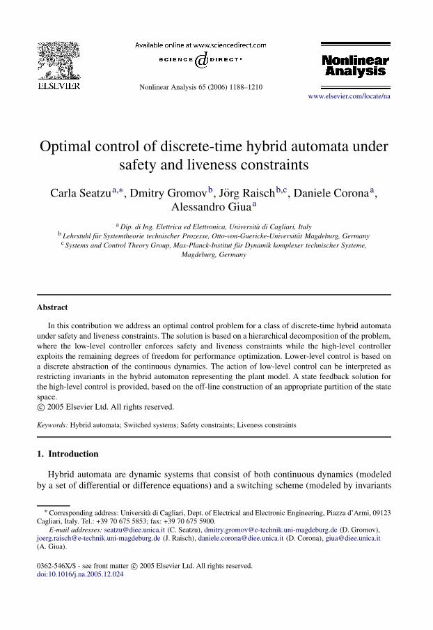
Fig. 7. Switching table of the problem OP(HA) defined in the example.

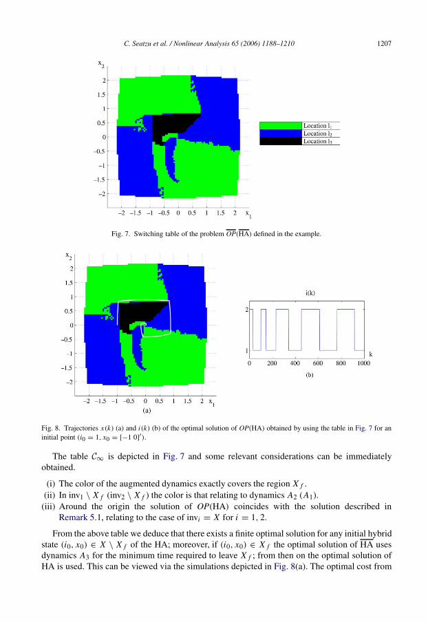
Fig. 8. Trajectories x(k) (a) and i(k) (b) of the optimal solution of OP(HA) obtained by using the table in Fig. 7 for aninitial point (i0 = 1, x0 = [−1 0]′).

The table C∞ is depicted in Fig. 7 and some relevant considerations can be immediatelyobtained.

(i) The color of the augmented dynamics exactly covers the region X f .(ii) In inv1 \ X f (inv2 \ X f ) the color is that relating to dynamics A2 (A1).

(iii) Around the origin the solution of OP(HA) coincides with the solution described inRemark 5.1, relating to the case of invi = X for i = 1, 2.

From the above table we deduce that there exists a finite optimal solution for any initial hybridstate (i0, x0) ∈ X \ X f of the HA; moreover, if (i0, x0) ∈ X f the optimal solution of HA usesdynamics A3 for the minimum time required to leave X f ; from then on the optimal solution ofHA is used. This can be viewed via the simulations depicted in Fig. 8(a). The optimal cost from


the point (i0 = 1, x0 = [−1 0]′) is J = 196.6. For completeness the index trajectory i(k) is alsoreported in Fig. 8(b).

The total computational time (Matlab 7, on an Intel Pentium 4 with 2 GHz and 256 MbRAM) for constructing the table in Fig. 7 is about 40 h. This time is large, because a very densespace discretization was considered (approximately 2 × 103 points). It is important, however,to point out that this computational effort is off-line. The on-line part of the procedure consistsin measuring the hybrid state (i(k), x(k)) and comparing its value with the switching table todecide on the optimal strategy.

6. Conclusion

We addressed the problem of designing a feedback control law for a discrete-time hybridautomaton HA. We showed that this law can be designed so that the system’s behavior satisfiestwo levels of specifications. The low-level specification prescribes liveness and safety conditionsfor the HA. We showed that the action of the low-level controller can be implemented restrictingthe invariants of HA. The high-level specification deals with the optimization of the trajectories:within the degree of freedom left by the low-level task, for a given initial state the high-level task finds the evolution that minimizes a given performance index. The robustness ofthe procedure has also been discussed. One perspective of interest for future developments isproviding structural conditions of the HA that guarantee the existence of admissible optimalcontrol laws.

Acknowledgement

This work was partially done in the framework of the HYCON Network of Excellence,contract number FP6-IST-511368.

Appendix A. Proof of Proposition 4.7

Let us first introduce some preliminary results.

Property 6.1. Let N, N ′ ∈ N. If N < N ′ and the switched system evolves along an optimaltrajectory, then for any continuous initial state x0, and for all i, j ∈ L,

+∞ > V ∗N (i, x0) ≥ V ∗

N ′ ( j, x0).

Proof. We first observe that by Assumptions 4.1 and 4.2 V ∗N (i, x0) is finite for any N ≥ 1. In

fact, regardless of the value of the initial dynamics i and the continuous state x0, we can alwaysswitch to the stable dynamics whose cost to infinity is finite. Now, we prove the second inequalityby contradiction. Assume that ∃ j ∈ L such that V ∗

N ′ ( j, x0) > V ∗N (i, x0). Then it is obvious that

the same evolution that generates V ∗N (i, x0) is also admissible for (11) starting from ( j, x0) when

a larger number N ′ of switches is allowed (it is sufficient to switch immediately from mode j tomode i ). This leads to a contradiction.

Proposition 6.2. Given a continuous initial state x0, for any ε′ > 0, there exists N = N(x0) ∈ N

such that for all N > N , V ∗N (i, x0) − V ∗

N( j, x0) < ε′ for all i, j ∈ L.


Proof. By definition V ∗N (i, x0) ≥ 0 for all i ∈ L, hence V ∗

N is a lower-bounded nonincreasingsequence (by Property 6.1). By the Axiom of Completeness it converges in R, hence it is aCauchy sequence.

Now, the statement of Proposition 4.7 can be proved.We first observe that by Assumption 4.6 V ∗

N (i, x0) is lower bounded by a strictly positivenumber. Moreover, the optimal costs are quadratic functions of x0, i.e., if x0 = λy0, thenV ∗

N (i, λy0) = λ2V ∗N (i, y0). Finally, by Proposition 6.2 ∀ y0 and ∀ ε′ > 0, ∃ N(y0) such that

∀ N > N (y0), V ∗N (i, y0) − V ∗

N( j, y0) < ε′. Hence if we define

N = maxy0:‖y0‖=1

N(y0) ⇒V ∗

N (i, x0) − V ∗N

( j, x0)

V ∗N (i, x0)

= λ2[V ∗N (i, y0) − V ∗

N( j, y0)]

λ2V ∗N (i, y0)

≤ ε′

miny0:‖y0‖=1

V ∗N (i, y0)

= ε.

References

[1] R. Alur, D.L. Dill, A theory of timed automata, in: Theoretical Computer Science, 1994.[2] E. Asarin, O. Bournez, T. Dang, O. Maler, A. Pnueli, Effective synthesis of switching controllers for linear systems,

Proceedings of the IEEE 88 (7) (2000).[3] P.E. Caines, R. Greiner, S. Wang, Dynamical logic observers for finite automata, in: Proceedings of the 27th

Conference on Decision and Control, Austin, Texas, 1988, pp. 226–233.[4] D. Corona, A. Giua, C. Seatzu, Optimal control of hybrid automata: an application to the design of a semiactive

suspension, Control Engineering Practice 12 (2004) 1305–1318.[5] D. Corona, A. Giua, C. Seatzu, Optimal feedback switching laws for autonomous hybrid automata, in: Proc. IEEE

Int. Sym. on Intelligent Control, Taipei, Taiwan, 2004.[6] D. Corona, A. Giua, C. Seatzu, Stabilization of switched system via optimal control, in: Proceedings of 16th IFAC

World Congress, Praga, Czech Republic, 2005.[7] D. Corona, C. Seatzu, A. Giua, D. Gromov, E. Mayer, J. Raisch, Optimal hybrid control for switched affine systems

under safety and liveness constraints, in: Proceedings of CACSD’05, Taipei, Taiwan, 2004.[8] J.E.R. Cury, B.H. Krogh, T. Niinomi, Synthesis of supervisory controllers for hybrid systems based on

approximating automata, IEEE Transactions on Automatic Control 43 (4) (1998) 564–568.[9] D. Gromov, E. Mayer, J. Raisch, D. Corona, C. Seatzu, A. Giua, Optimal control of discrete time hybrid automata

under safety and liveness constraints, in: ISIC, Limassol, Cyprus, June 2005.[10] S. Hedlund, A. Rantzer, Convex dynamic programming for hybrid systems, IEEE Transactions on Automatic

Control 47 (9) (2002) 1536–1540.[11] T. Moor, J. Raisch, Supervisory control of hybrid systems within a behavioural framework, Hybrid Control Systems,

Systems and Control Letters 38 (1999) 157–166 (special issue).[12] X. Nicollin, A. Olivero, J. Sifakis, S. Yovine, An approach to the description and analysis of hybrid systems,

in: Hybrid Systems, in: LNCS, vol. 736, Springer Verlag, 1993.[13] Cuneyt M. Ozveren, Allan S. Willsky, Observability of discrete event dynamic systems, IEEE Transaction on

Automatic Control 35 (7) (1990) 797–806.[14] B. Piccoli, Necessary conditions for hybrid optimization, in: Proc. 38th IEEE Conf. on Decision and Control,

Phoenix, Arizona USA, December 1999.[15] J. Raisch, Discrete abstractions of continuous systems — an input/output point of view, Discrete Event Models of

Continuous Systems, Mathematical and Computer Modelling of Dynamical Systems 6 (2000) 6–29 (special issue).[16] J. Raisch, S. O’Young, Discrete approximation and supervisory control of continuous systems, IEEE Transactions

on Automatic Control 43 (4) (1998) 569–573.


[17] P.J. Ramadge, W.M. Wonham, The control of discrete event systems, Discrete Event Dynamic Systems. Proceedingsof the IEEE 77 (1) (1989) 81–98 (special issue).

[18] P. Riedinger, F. Kratz, C. Iung, C. Zanne, Linear quadratic optimization for hybrid systems, in: Proc. 38th IEEEConf. on Decision and Control, Phoenix, USA, December 1999, pp. 3059–3064.

[19] J. Schroder, Modelling, State Observation and Diagnosis of Quantised Systems, Springer-Verlag, 2002.[20] C. Seatzu, D. Corona, A. Giua, A. Bemporad, Optimal control of continuous-time switched affine systems, IEEE

Transactions on Automatic Control (2005) (in press).[21] M.S. Shaikh, P.E. Caines, On the optimal control of hybrid systems: analysis and algorithms for trajectory and

scheduled optimization, Hawaii, USA, December 2003, pp. 2144–2149.[22] H.J. Sussmann, A maximum principle for hybrid optimal control problems, in: Proc. 38th IEEE Conf. on Decision

and Control, Phoenix, USA, December 1999, pp. 425–430.[23] J.C. Willems, Models for dynamics, Dynamics Reported 2 (1989).[24] X. Xu, P.J. Antsaklis, An approach to switched systems optimal control based on parameterization of the switching

instants, in: Proc. IFAC World Congress, Barcelona, Spain, 2002.[25] X. Xu, P.J. Antsaklis, Results and perspectives on computational methods for optimal control of switched systems,

in: Hybrid Systems, Computation and Control, Prague, Czech Republic, 2003.

optimal control of discrete-time hybrid automata under ...€¦ · optimal control of discrete-time...

Documents