optimal control and mpc for the fokker-planck equation · optimal control and mpc for the...
TRANSCRIPT

Optimal Control and MPCfor the Fokker-Planck equation
Roberto Guglielmi
University of Bayreuth, Germany& Imperial College London, UK
SADCO Internal Review MeetingNew Perspectives in Optimal Control and Games
Dipartimento di Matematica - Universita di Roma ”La Sapienza”
November 10, 2014 - Rome, Italy
R. Guglielmi (Uni Bayreuth & ICL) [email protected] November 10, 2014 1 / 34

Outline
1 Motivation
2 Model Predictive Control
3 Existing Works
4 New Results
5 Outlook
R. Guglielmi (Uni Bayreuth & ICL) [email protected] November 10, 2014 2 / 34

Outline
1 Motivation
2 Model Predictive Control
3 Existing Works
4 New Results
5 Outlook
R. Guglielmi (Uni Bayreuth & ICL) [email protected] November 10, 2014 2 / 34

Outline
1 Motivation
2 Model Predictive Control
3 Existing Works
4 New Results
5 Outlook
R. Guglielmi (Uni Bayreuth & ICL) [email protected] November 10, 2014 2 / 34

Outline
1 Motivation
2 Model Predictive Control
3 Existing Works
4 New Results
5 Outlook
R. Guglielmi (Uni Bayreuth & ICL) [email protected] November 10, 2014 2 / 34

Outline
1 Motivation
2 Model Predictive Control
3 Existing Works
4 New Results
5 Outlook
R. Guglielmi (Uni Bayreuth & ICL) [email protected] November 10, 2014 2 / 34

Outline
1 Motivation
2 Model Predictive Control
3 Existing Works
4 New ResultsThe Influence of the Horizon NSpace- (and Time-)Dependent Control u(x , t)
5 Outlook
R. Guglielmi (Uni Bayreuth & ICL) [email protected] November 10, 2014 3 / 34

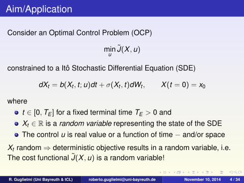
Aim/Application
Consider an Optimal Control Problem (OCP)
minu
J(X ,u)
constrained to a Ito Stochastic Differential Equation (SDE)
dXt = b(Xt , t ; u)dt + σ(Xt , t)dWt , X (t = 0) = x0
wheret ∈ [0,TE ] for a fixed terminal time TE > 0 andXt ∈ R is a random variable representing the state of the SDEThe control u is real value or a function of time − and/or space
Xt random⇒ deterministic objective results in a random variable, i.e.The cost functional J(X ,u) is a random variable!
R. Guglielmi (Uni Bayreuth & ICL) [email protected] November 10, 2014 4 / 34

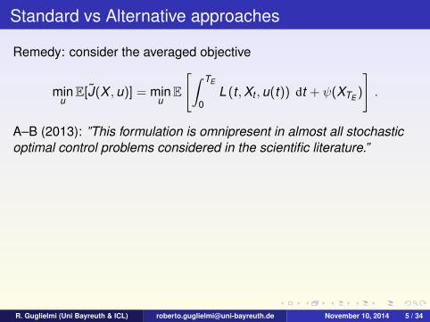
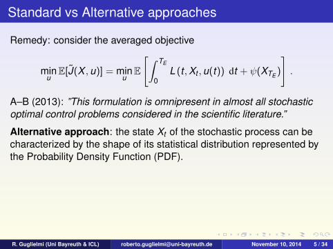
Standard vs Alternative approaches
Remedy: consider the averaged objective
minu
E[J(X ,u)] = minu
E
[∫ TE
0L (t ,Xt ,u(t)) dt + ψ(XTE )
].
A–B (2013): ”This formulation is omnipresent in almost all stochasticoptimal control problems considered in the scientific literature.”
Alternative approach: the state Xt of the stochastic process can becharacterized by the shape of its statistical distribution represented bythe Probability Density Function (PDF).Related works: deterministic objectives defined by the Kullback-Leiblerdistance (G. Jumarie 1992, M. Karny 1996) or the square distance(M.G. Forbes, M. Guay, J.F. Forbes 2004, Wang 1999) between thestate PDF and a desired one. However, stochastic models needed toobtain the PDF by averaging or by an interpolation
R. Guglielmi (Uni Bayreuth & ICL) [email protected] November 10, 2014 5 / 34
Standard vs Alternative approaches
Remedy: consider the averaged objective
minu
E[J(X ,u)] = minu
E
[∫ TE
0L (t ,Xt ,u(t)) dt + ψ(XTE )
].
A–B (2013): ”This formulation is omnipresent in almost all stochasticoptimal control problems considered in the scientific literature.”
Alternative approach: the state Xt of the stochastic process can becharacterized by the shape of its statistical distribution represented bythe Probability Density Function (PDF).
Related works: deterministic objectives defined by the Kullback-Leiblerdistance (G. Jumarie 1992, M. Karny 1996) or the square distance(M.G. Forbes, M. Guay, J.F. Forbes 2004, Wang 1999) between thestate PDF and a desired one. However, stochastic models needed toobtain the PDF by averaging or by an interpolation
R. Guglielmi (Uni Bayreuth & ICL) [email protected] November 10, 2014 5 / 34

Standard vs Alternative approaches
Remedy: consider the averaged objective
minu
E[J(X ,u)] = minu
E
[∫ TE
0L (t ,Xt ,u(t)) dt + ψ(XTE )
].
A–B (2013): ”This formulation is omnipresent in almost all stochasticoptimal control problems considered in the scientific literature.”
Alternative approach: the state Xt of the stochastic process can becharacterized by the shape of its statistical distribution represented bythe Probability Density Function (PDF).Related works: deterministic objectives defined by the Kullback-Leiblerdistance (G. Jumarie 1992, M. Karny 1996) or the square distance(M.G. Forbes, M. Guay, J.F. Forbes 2004, Wang 1999) between thestate PDF and a desired one. However, stochastic models needed toobtain the PDF by averaging or by an interpolation
R. Guglielmi (Uni Bayreuth & ICL) [email protected] November 10, 2014 5 / 34

The Fokker-Planck Equation /1
A new approach by Annunziato and Borzı (2010, 2013):Reformulate the objective using the underlying PDF
y(x , t) :=
∫Ω
y(x , t ; z,0)ρ(z,0)dz
t > 0, ρ(z,0) given initial density probability,y transition density probability distribution function
y(x , t ; z, s) := PX (t) ∈ (x , x + dx) : X (s) = z , t > s
and control the PDF directly.
The next essential step:the evolution of the PDF is governed by (cf Da Prato - Zabczyk) theFokker-Planck Equation (deterministic parabolic PDE)
R. Guglielmi (Uni Bayreuth & ICL) [email protected] November 10, 2014 6 / 34
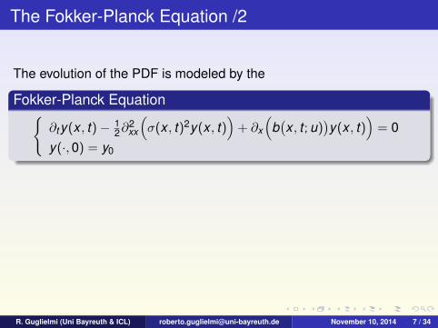
The Fokker-Planck Equation /2
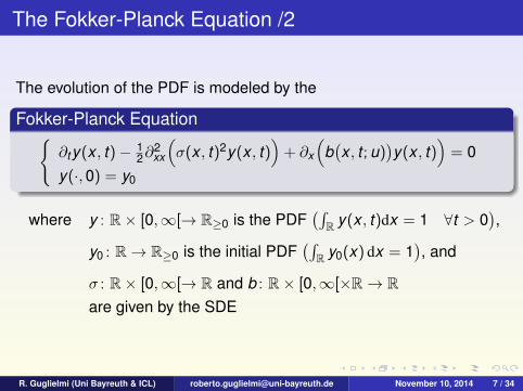
The evolution of the PDF is modeled by the
Fokker-Planck Equation∂ty(x , t)− 1
2∂2xx
(σ(x , t)2y(x , t)
)+ ∂x
(b(x , t ; u)
)y(x , t)
)= 0
y(·,0) = y0
where y : R× [0,∞[→ R≥0 is the PDF(∫
R y(x , t)dx = 1 ∀t > 0),
y0 : R→ R≥0 is the initial PDF(∫
R y0(x) dx = 1), and
σ : R× [0,∞[→ R and b : R× [0,∞[×R→ Rare given by the SDE
R. Guglielmi (Uni Bayreuth & ICL) [email protected] November 10, 2014 7 / 34
The Fokker-Planck Equation /2
The evolution of the PDF is modeled by the
Fokker-Planck Equation∂ty(x , t)− 1
2∂2xx
(σ(x , t)2y(x , t)
)+ ∂x
(b(x , t ; u)
)y(x , t)
)= 0
y(·,0) = y0
where y : R× [0,∞[→ R≥0 is the PDF(∫
R y(x , t)dx = 1 ∀t > 0),
y0 : R→ R≥0 is the initial PDF(∫
R y0(x) dx = 1), and
σ : R× [0,∞[→ R and b : R× [0,∞[×R→ Rare given by the SDE
R. Guglielmi (Uni Bayreuth & ICL) [email protected] November 10, 2014 7 / 34

A MPC−Fokker-Planck control framework
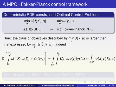
Deterministic PDE-constrained Optimal Control Problem
minu
E[J(X ,u)] minu
J(y ,u)
s.t. Ito SDE s.t. Fokker-Planck PDE
Rmk: the class of objectives described by minu
J(y ,u) is larger then
that expressed by minu
E[J(X ,u)], indeed
E
TE∫0
L(t ,Xt ,u(t)) + ψ(XTE )
=
∫Rd
TE∫0
L(t , x ,u(t))y(t , x)+
∫Rdψ(x)y(TE , x) .
Control method: Model Predictive Control (MPC)
R. Guglielmi (Uni Bayreuth & ICL) [email protected] November 10, 2014 8 / 34
A MPC−Fokker-Planck control framework
Deterministic PDE-constrained Optimal Control Problem
minu
E[J(X ,u)] minu
J(y ,u)
s.t. Ito SDE s.t. Fokker-Planck PDE
Rmk: the class of objectives described by minu
J(y ,u) is larger then
that expressed by minu
E[J(X ,u)], indeed
E
TE∫0
L(t ,Xt ,u(t)) + ψ(XTE )
=
∫Rd
TE∫0
L(t , x ,u(t))y(t , x)+
∫Rdψ(x)y(TE , x) .
Control method: Model Predictive Control (MPC)
R. Guglielmi (Uni Bayreuth & ICL) [email protected] November 10, 2014 8 / 34

Outline
1 Motivation
2 Model Predictive Control
3 Existing Works
4 New ResultsThe Influence of the Horizon NSpace- (and Time-)Dependent Control u(x , t)
5 Outlook
R. Guglielmi (Uni Bayreuth & ICL) [email protected] November 10, 2014 9 / 34

Basic idea of MPC
OCP on a long Several iterative OCPs(possibly infinite) on (shorter) finite
time horizon time horizons
R. Guglielmi (Uni Bayreuth & ICL) [email protected] November 10, 2014 10 / 34
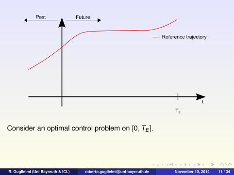
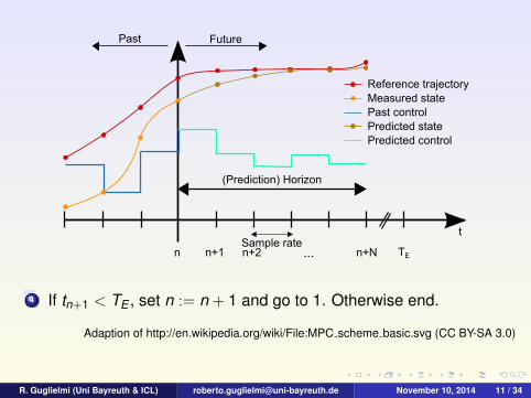
Past Future
t
TE
Reference trajectory
Consider an optimal control problem on [0,TE ].
R. Guglielmi (Uni Bayreuth & ICL) [email protected] November 10, 2014 11 / 34

Past Future
t
TE
Reference1trajectoryMeasured1statePast1control
...Sample1rate
(Prediction)1Horizon
n n+1 n+2 n+N
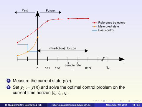
Choose a horizon N ∈ N and a sample rate T > 0.For each time tn := nT ,n = 0,1,2, ... :
R. Guglielmi (Uni Bayreuth & ICL) [email protected] November 10, 2014 11 / 34
Past Future
t
TE
Reference1trajectoryMeasured1statePast1control
...Sample1rate
(Prediction)1Horizon
n n+1 n+2 n+N
1 Measure the current state y(n).2 Set y0 := y(n) and solve the optimal control problem on the
current time horizon [tn, tn+N ].
R. Guglielmi (Uni Bayreuth & ICL) [email protected] November 10, 2014 11 / 34

Past Future
t
TE
Reference1trajectoryMeasured1statePast1controlPredicted1statePredicted1control
...Sample1rate
(Prediction)1Horizon
n n+1 n+2 n+N
3 Denote the calculated optimal control sequence by u∗(·) andapply its first value u∗(0) on [tn, tn+1].
R. Guglielmi (Uni Bayreuth & ICL) [email protected] November 10, 2014 11 / 34
Past Future
t
TE
Reference1trajectoryMeasured1statePast1controlPredicted1statePredicted1control
...Sample1rate
(Prediction)1Horizon
n n+1 n+2 n+N
4 If tn+1 < TE , set n := n + 1 and go to 1. Otherwise end.
Adaption of http://en.wikipedia.org/wiki/File:MPC scheme basic.svg (CC BY-SA 3.0)
R. Guglielmi (Uni Bayreuth & ICL) [email protected] November 10, 2014 11 / 34

Outline
1 Motivation
2 Model Predictive Control
3 Existing Works
4 New ResultsThe Influence of the Horizon NSpace- (and Time-)Dependent Control u(x , t)
5 Outlook
R. Guglielmi (Uni Bayreuth & ICL) [email protected] November 10, 2014 12 / 34

Existing Work
Problem [Annunziato and Borzı, 2010, 2013]Track a desired PDF over a given time interval.
Optimal Control Problem
Ω ⊂ R open interval, ua,ub ∈ R with ua < ub, yd ∈ L2(Ω) and λ > 0.Consider the following OCP on [tn, tn+1]:
minu
J(y ,u) :=12‖y(·, tn+1)− yd (·, tn+1)‖2L2(Ω) +
λ
2|u|2
s.t.∂ty − 1
2∂2xx(σ2y
)+ ∂x (b(u)y) = 0 in Qn := Ω× (tn, tn+1)
y(·, tn) = yn in Ωy = 0 in Σn := ∂Ω× (tn, tn+1)
(1)
u ∈ Uad := u ∈ R |ua ≤ u ≤ ub
R. Guglielmi (Uni Bayreuth & ICL) [email protected] November 10, 2014 13 / 34

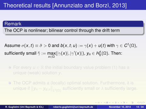
Theoretical results [Annunziato and Borzı, 2013]
RemarkThe OCP is nonlinear; bilinear control through the drift term
Assume σ(x , t) ≡ σ > 0 and b(x , t ; u) := γ(x) + u(t) with γ ∈ C1(Ω),
sufficiently small γ := maxx∈Ω
(|γ(x)|, |γ′(x)|), yn ∈ H10 (Ω). Then:
For every u ∈ R the initial boundary value problem (1) has aunique (weak) solution y .
The OCP admits a (locally) optimal solution. Furthermore, it isunique if
∥∥yn − yd ,n∥∥
L2(Ω)sufficiently small or λ sufficiently large.
R. Guglielmi (Uni Bayreuth & ICL) [email protected] November 10, 2014 14 / 34

Past Future
t
TE
Reference1trajectoryMeasured1statePast1controlPredicted1statePredicted1control
...Sample1rate
(Prediction)1Horizon
n n+1 n+2
Adaption of http://en.wikipedia.org/wiki/File:MPC scheme basic.svg (CC BY-SA 3.0)
R. Guglielmi (Uni Bayreuth & ICL) [email protected] November 10, 2014 15 / 34

A Fokker-Planck optimality system
N = 1: the first order necessary optimality conditions solve thefollowing optimality system
∂ty −12∂2
xx
(σ2y
)+ ∂x (b(u)y) = 0 in Qn
y(·, tn) = yn in Ω
y = 0 in Σn
−∂tp −12σ2∂2
xxp−b(u)∂xp = 0 in Qn
p(·, tn+1) = y(·, tn+1)− yd (·, tn+1) in Ω
p = 0 in Σn
λu −∫
Qn
∂x
(∂b∂u
y)
p dx dt = 0
R. Guglielmi (Uni Bayreuth & ICL) [email protected] November 10, 2014 16 / 34
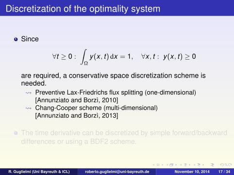
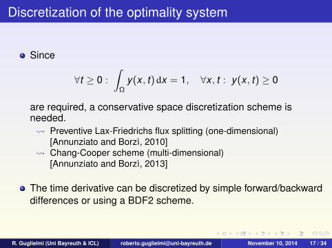
Discretization of the optimality system
Since
∀t ≥ 0 :
∫Ω
y(x , t) dx = 1, ∀x , t : y(x , t) ≥ 0
are required, a conservative space discretization scheme isneeded. Preventive Lax-Friedrichs flux splitting (one-dimensional)
[Annunziato and Borzı, 2010] Chang-Cooper scheme (multi-dimensional)
[Annunziato and Borzı, 2013]
The time derivative can be discretized by simple forward/backwarddifferences or using a BDF2 scheme.
R. Guglielmi (Uni Bayreuth & ICL) [email protected] November 10, 2014 17 / 34

Outline
1 Motivation
2 Model Predictive Control
3 Existing Works
4 New ResultsThe Influence of the Horizon NSpace- (and Time-)Dependent Control u(x , t)
5 Outlook
R. Guglielmi (Uni Bayreuth & ICL) [email protected] November 10, 2014 18 / 34

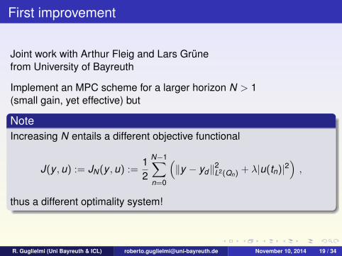
First improvement
Joint work with Arthur Fleig and Lars Grunefrom University of Bayreuth
Implement an MPC scheme for a larger horizon N > 1(small gain, yet effective) but
NoteIncreasing N entails a different objective functional
J(y ,u) := JN(y ,u) :=12
N−1∑n=0
(‖y − yd‖2L2(Qn) + λ|u(tn)|2
),
thus a different optimality system!
R. Guglielmi (Uni Bayreuth & ICL) [email protected] November 10, 2014 19 / 34

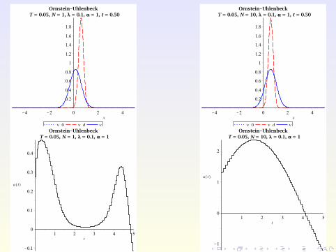
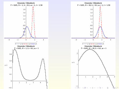
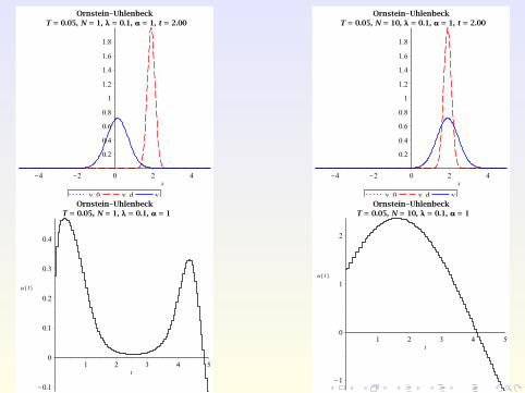
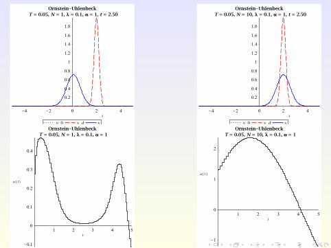
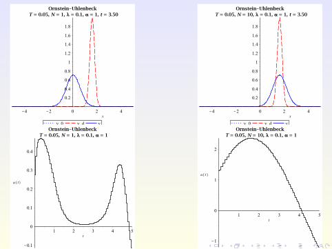
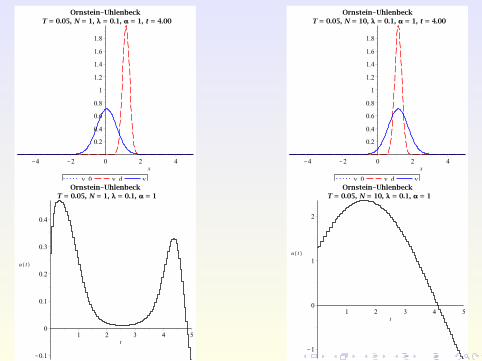
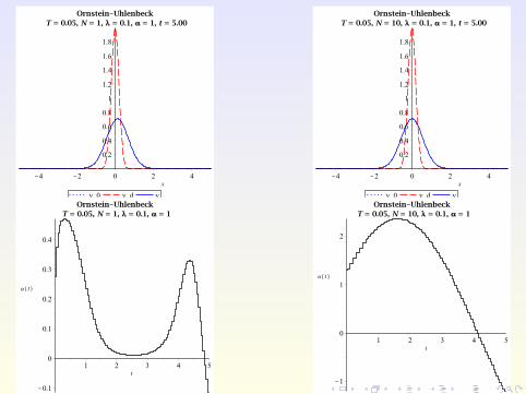
Numerical Example
Consider the Ornstein-Uhlenbeck process with
σ(x , t) ≡ σ = 0.8, b(x , t ,u) := u − x
on Ω :=]− 5,5[ with ua = −10,ub = 10, λ = 0.1, and TE = 5.
The target and initial PDF are given by
yd (x , t) :=exp
(− [x−2 sin(πt/5)]2
2·0.22
)√
2π · 0.22
and
y0(x) := yd (x ,0) =exp
(− x2
2·0.22
)√
2π · 0.22,
respectively.
R. Guglielmi (Uni Bayreuth & ICL) [email protected] November 10, 2014 20 / 34


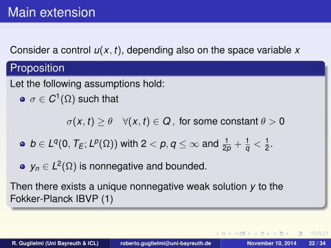
Main extension
Consider a control u(x , t), depending also on the space variable x
PropositionLet the following assumptions hold:
σ ∈ C1(Ω) such that
σ(x , t) ≥ θ ∀(x , t) ∈ Q , for some constant θ > 0
b ∈ Lq(0,TE ; Lp(Ω)) with 2 < p,q ≤ ∞ and 12p + 1
q <12 .
yn ∈ L2(Ω) is nonnegative and bounded.
Then there exists a unique nonnegative weak solution y to theFokker-Planck IBVP (1)
R. Guglielmi (Uni Bayreuth & ICL) [email protected] November 10, 2014 22 / 34
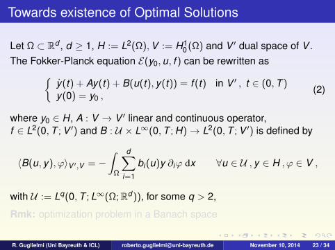
Towards existence of Optimal Solutions
Let Ω ⊂ Rd , d ≥ 1, H := L2(Ω),V := H10 (Ω) and V ′ dual space of V .
The Fokker-Planck equation E(y0,u, f ) can be rewritten asy(t) + Ay(t) + B(u(t), y(t)) = f (t) in V ′ , t ∈ (0,T )y(0) = y0 ,
(2)
where y0 ∈ H, A : V → V ′ linear and continuous operator,f ∈ L2(0,T ; V ′) and B : U × L∞(0,T ; H)→ L2(0,T ; V ′) is defined by
〈B(u, y), ϕ〉V ′,V = −∫
Ω
d∑i=1
bi(u)y ∂iϕ dx ∀u ∈ U , y ∈ H , ϕ ∈ V ,
with U := Lq(0,T ; L∞(Ω;Rd )), for some q > 2,
Rmk: optimization problem in a Banach space
R. Guglielmi (Uni Bayreuth & ICL) [email protected] November 10, 2014 23 / 34

A-priori estimates
Let y0 ∈ H, f ∈ L2(0,T ; V ′) and u ∈ U . Then a solution y of theFokker-Planck equation (2) satisfies the estimates
|y |2L∞(0,T ;H) ≤ Cec|u|2U[|y(0)|2H + |f |2L2(0,T ;V ′)
],
|y |2L2(0,T ;V ) ≤ C max(1, |u|2Uec|u|2U )(|y(0)|2H + |f |2L2(0,T ;V ′)
),
|y |2L2(0,T ;V ′) ≤ C(1 + |u|2Uec|u|2U )(|y(0)|2H + |f |2L2(0,T ;V ′)
)+ 2|f |2L2(0,T ;V ′) ,
for some positive constants c, C.
R. Guglielmi (Uni Bayreuth & ICL) [email protected] November 10, 2014 24 / 34

Existence and Uniqueness of Optimal Control
Let y0 ∈ V , yd ∈ H and J(u) := |y − yd |2L2(0,T ;H)+ λ|u|2U , λ > 0
where y is the unique solution toy(t) + Ay(t) + B(u(t), y(t)) = 0 in V ′ , t ∈ (0,T )y(0) = y0 ,
Then there exists a pair
(y , u) ∈ C([0,T ],H)× U
such that y is a solution of E(y0, u,0) and u minimizes J in U .
Moreover, pair (y , u) unique for small |y − yd |L2(0,T ;H) or for large λ
R. Guglielmi (Uni Bayreuth & ICL) [email protected] November 10, 2014 25 / 34
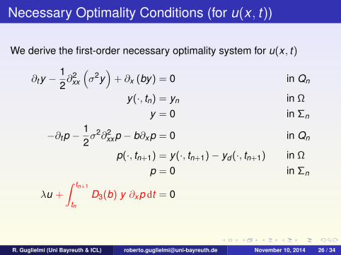
Necessary Optimality Conditions (for u(x , t))
We derive the first-order necessary optimality system for u(x , t)
∂ty −12∂2
xx
(σ2y
)+ ∂x (by) = 0 in Qn
y(·, tn) = yn in Ω
y = 0 in Σn
−∂tp −12σ2∂2
xxp − b∂xp = 0 in Qn
p(·, tn+1) = y(·, tn+1)− yd (·, tn+1) in Ω
p = 0 in Σn
λu +
∫ tn+1
tnD3(b) y ∂xp dt = 0
R. Guglielmi (Uni Bayreuth & ICL) [email protected] November 10, 2014 26 / 34

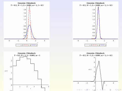
Numerical Examples
Consider the Ornstein-Uhlenbeck process from before, but withspace-dependent control u(x , t) and λ = 0.001 instead of 0.1.
R. Guglielmi (Uni Bayreuth & ICL) [email protected] November 10, 2014 27 / 34

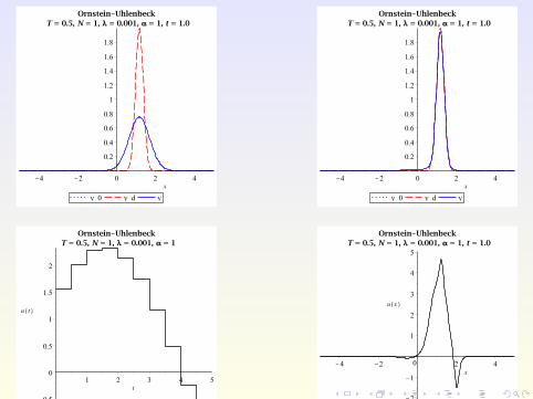

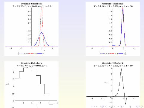


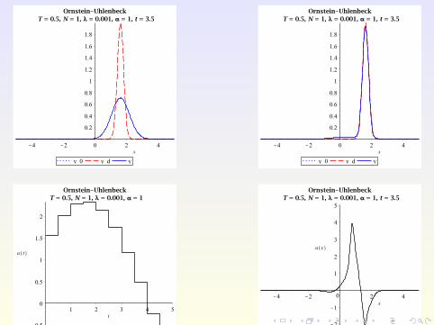
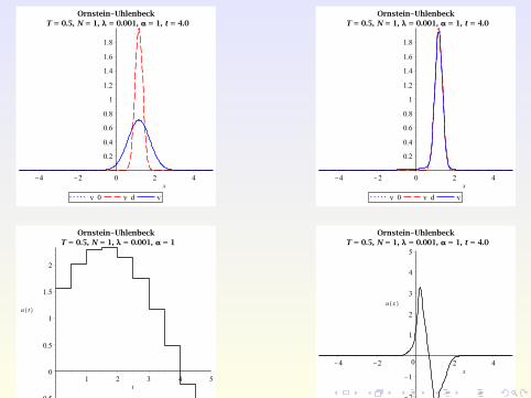
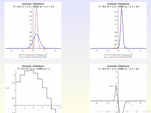
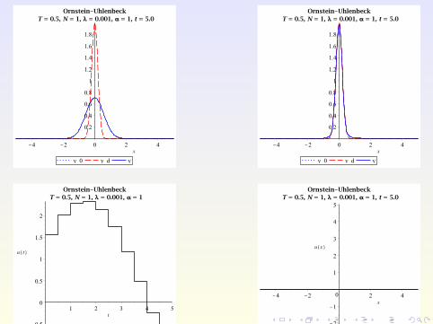

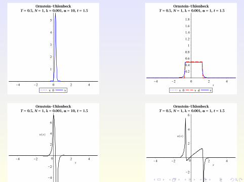
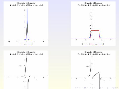
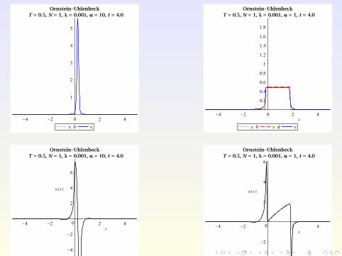
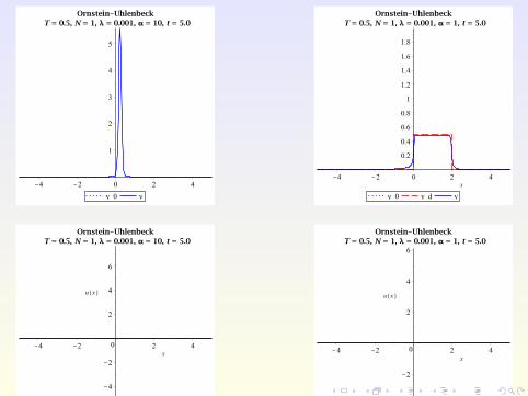
Numerical Examples (2)
With space-dependent control, larger class of objectives possible:
region avoidance, without prescribing the shape of the PDF,e.g. try to force the state PDF into [0,0.5].
Try to track non-smooth targets, e.g.
yd (x , t) :=
0.5 if x ∈ [−1 + 0.15t ,1 + 0.15t ]0 otherwise.
R. Guglielmi (Uni Bayreuth & ICL) [email protected] November 10, 2014 29 / 34


Outline
1 Motivation
2 Model Predictive Control
3 Existing Works
4 New ResultsThe Influence of the Horizon NSpace- (and Time-)Dependent Control u(x , t)
5 Outlook
R. Guglielmi (Uni Bayreuth & ICL) [email protected] November 10, 2014 31 / 34

Some remarks
– Numerical simulations also for the Geometric-Brownian processand the Shiryaev process
– The computed optimal control of the PDF is then applied to thestochastic process
– Right boundary conditions of Robin type
– The same Fokker-Planck Optimal Control framework applies to- the class of piecewise deterministic processes- optimal control of open quantum systems- subdiffusion processes
R. Guglielmi (Uni Bayreuth & ICL) [email protected] November 10, 2014 32 / 34

Outlook
The Influence of the Horizon NUse known techniques from, e.g. [Altmuller and Grune, 2012], inorder to find estimates for horizons N that guarantee stability of theMPC closed-loop system.
Space- (and Time-)Dependent Control u(x , t)Controllability of the Fokker-Planck equation (2):Compare with previous work by
Blaquiere 1992( continuous initial datum and final target with compactsupport in 1D)
and the recent result byPorretta 2014
( continuously differentiable PDFs that are strictly positiveeverywhere).
R. Guglielmi (Uni Bayreuth & ICL) [email protected] November 10, 2014 33 / 34

Thank you for your attention!
R. Guglielmi (Uni Bayreuth & ICL) [email protected] November 10, 2014 34 / 34