Optimal Compression of a Polylinewith Segments and Arcs

Alexander GribovEsri

380 New York StreetRedlands, CA 92373

Email: agribov@esri.com

Abstract

This paper describes an efficient approach to constructing a resultant polyline with a minimum number of segments and arcs.While fitting an arc can be done with complexity O(1) (see [1] and [2]), the main complexity is in checking that the resultant arcis within the specified tolerance. There are additional tests to check for the ends and for changes in direction (see [3, section 3]and [4, sections II.C and II.D]). However, the most important part in reducing complexity is the ability to subdivide the polylinein order to limit the number of arc fittings [2]. The approach described in this paper finds a compressed polyline with a minimumnumber of segments and arcs.

Index Terms

polyline compression; polyline approximation; arc fitting; generalization; minimum width annulus; the closest Delaunaytriangulation; the farthest Delaunay triangulation; inversive geometry; rational geometry; plane sweep algorithm

I. INTRODUCTION

Compression of a polyline with a minimum number of segments, within a specified tolerance, is described in [5]. [6] findsa compressed polyline with the minimum number of arcs with complexity O

(N3), where N is the number of vertices in the

source polyline. Another algorithm described in [7] has lower complexity O(N2 log (N)

); however, it might not be applicable

for all cases, for example, when there is a backward movement in the source polyline along the true unknown arc. Thesealgorithms construct a resultant polyline from the subset of the vertices of the source polyline. It is possible to achieve a highercompression ratio and better error filtering when vertices of the resultant polyline are not required to be from the subset ofthe vertices of the source polyline [4].

To find the optimal solution, the dynamic programming approach is applied (see [5], [6], [8], [9], [10], and [4]). In the caseof straight segments, the reduction of the search in the dynamic programming approach is done by using the convex hull [11].Parts of the polyline having a minimum width of the convex hull more than twice that of the specified tolerance are excludedfrom the analysis. This paper describes an approach to reduce the search in the dynamic programming approach for arcs. Ifpart of the polyline cannot be fitted with an arc, then any part of the polyline containing that part can be skipped duringanalysis. The example in [2] uses this approach; however, the test is approximate.

II. FINDING A COMPRESSED POLYLINE WITH A MINIMUM NUMBER OF SEGMENTS AND ARCS

The task to find a compressed polyline with a minimum number of segments and arcs is solved by dynamic programming[6], [9], and [4]. Allowing the resultant vertices to be different from the vertices of the source polyline improves compression[4]. The algorithm in [4] places a finite number of points around each vertex of the source polyline and searches for theresultant polyline connecting these points.

Table I compares the differences between segments and arcs when vertices of the resultant polyline are the subset of thevertices of the source polyline or when using the approach from [4].

For fitting arcs by least deviation, it is possible to reduce complexity by using polygons obtained as the intersection ofthe closest and the farthest Voronoi diagrams (see section II-A “Finding a Smallest-Width Annulus”). The test for geometricprimitives to be within the specified tolerance requires finding the closest and the farthest points from the center. Note that theclosest point should belong to the alpha shape with the generalized disk radius equal to or less than the radius of the checkedarc, and the farthest point should belong to the convex hull.

Let Pi,j , 0 ≤ i ≤ j < N be parts of the source polyline from vertex i to j, where N is the total number of vertices. Theoptimal solution is found by induction. First, define the solution for polyline P0,0. Second, for k = 1..N − 1, construct theoptimal solution for P0,k from optimal solutions for P0,k′ , k′ = 0..k − 1. However, it is not always necessary to search overall k′ because, for some isegment(k) and iarc(k), either there are no segments for Pisegment(k),k or no arcs for Piarc(k),k existwithin the specified tolerance. It is sufficient to search only for segments for k′ = isegment(k) + 1..k − 1 and for arcs for

arX

iv:1

604.

0747

6v5

[cs

.CG

] 1

0 A

pr 2

017

TABLE ICOMPLEXITY COMPARISON FOR EVALUATION SEGMENTS AND ARCS

WHEN END POINTS ARE KNOWN AND n POINTS ARE BETWEEN THE END POINTS.

Segment ArcFitting by least squares approach Complexity O(1), connect start and end points O(1), see [2]

for approximate solutionFitting by least deviation Complexity O(1), connect start and end points Complexity O(n log (n)),

see Appendix I “Fitting an Arc by Tolerance”Check if the geometric primitive Complexity O(log (n)), using convex hull, see [11] Complexity O(n),is within the specified tolerance (this paper will use the algorithm with complexity O

(log2 (n)

), need to check every vertex

see Appendix II “Efficient Tolerance Checking of a Segment”)Testing end points and direction, Complexity O(log (n)) (this paper will use the algorithm Complexity O(n),see [4] and [3, section 3] with complexity O

(log2 (n)

), see need to check every vertex

Appendix II “Efficient Tolerance Checking of a Segment”)and O(1), respectively, see [4]

k′ = iarc(k) + 1..k − 31. The task of finding iarc(k) is described in Appendix III “Testing Parts of The Source Polyline forArc Fitting”. A similar algorithm can be used to find isegment(k).

A. Finding a Smallest-Width Annulus

The task of checking if an arc exists that covers all points within the specified tolerance has an exact solution, describedin [12, section 7.4]. From [2, section VII]: The solution is found using the closest and the farthest point Voronoi diagrams.The center of an arc corresponding to the minimum width covering all vertices is either a vertex of the closest or the farthestpoint Voronoi diagram, or a point on the edge of the closest and the farthest point Voronoi diagrams [12, p. 167]. The closestand the farthest point Voronoi diagrams are dual with the closest and the farthest point Delaunay triangulations, respectively[13]. Note that the farthest point Voronoi diagram includes only vertices on the convex hull.2

In Appendix IV “Duality of the Farthest and the Closest Delaunay Diagrams by Inversive Geometry”, it will be shownthat the farthest Delaunay triangulation is dual to the closest Delaunay triangulation for the inverted set of points. This givesthe possibility to reuse the existing implementation of the closest Delaunay triangulation to construct the farthest Delaunaytriangulation and the farthest Voronoi diagram. It also shows that the algorithms for calculation of the closest Delaunaytriangulation can be modified to calculate the farthest Delaunay triangulation.

From [2, section VII]: Another algorithm to construct the closest and the farthest point Delaunay triangulations for verticeson the convex hull is by mapping each vertex (x, y) to a vertex in three-dimensional space

(x, y, x2 + y2

)and constructing a

convex hull for them [13].Construction of the closest and the farthest Delaunay triangulation can be implemented by the divide-and-conquer algorithm

described in [14] and [15]. While modification of this algorithm described in [16] has complexity O(N log (log (N))) foruniformly distributed data, there is no algorithm available for the non-uniformly distributed data. However, alternating horizontaland vertical directions (whichever is longer) when dividing data into two almost equal parts by recursively using the quicksort algorithm produces a faster algorithm with average complexity O(N log (N)) [17]. To achieve worst-case complexityO(N log (N)), it is necessary to achieve worst-case complexity O(N) in finding the median, which is achievable by using themedian of medians algorithm, see [18, section 9.3]. Note that construction of the closest or the farthest Delaunay triangulationby use of the flipping algorithm results in the worst-case complexity of O

(N2), see proof in [14], [17], and [19].

Adding an infinite point to the Delaunay triangulation makes the number of edges equal to 3 (n− 1), for n > 1 and oneedge for one point, where n is the number of points not counting the infinite point. This construction simplifies the divide-and-conquer algorithm, as there is no requirement to have at least two points in both Delaunay triangulations as requiredin [15]. Note that neighboring convex hull edges are always separated by an edge to the infinite point. That infinite pointis considered to be always outside of any circle in Delaunay triangulation. This paper will follow the divide-and-conqueralgorithm described in [14]. The first step in merging two Delaunay triangulations is to find lower and upper common tangentsas in [14]. There is a special case where the lower and upper common tangents are the same. This happens when all pointsare on the line. In such a case, an extra connection to the infinite point is added for each Delaunay triangulation, unless ithas only one point, and one edge is added to connect two Delaunay triangulations. The second step in merging two Delaunaytriangulations is finding first the left and right points to be hit, see [14] and [15]. Note that in this step, there is no need to

1At least three points are necessary in order to fit an arc. However, any three points can be fitted with an arc passing through them. Therefore, to avoidgeneration of too many arcs, this algorithm will require at least four points.

2Delaunay triangulation has an exact solution in integer arithmetic. There is also an exact solution in real arithmetic, because any real number can be exactlyrepresented as a rational number. Both implementations require the use of extended precision. The Voronoi diagram also has an exact solution; however, thevertices of the Voronoi diagram are rational numbers. In the case of Delaunay triangulation on real or even integer numbers, interval arithmetic can be usedto decide if extended precision is necessary.

2

perform the test to check if the point is above the base edge, because the test to check if a point is inside a circle (performedby finding a sign of the determinant (2), see [15]), will eliminate all cases where a point is not above the base edge. Byproving that all cases will be processed in the same way without this test, it follows that this test can be skipped. There arefour possible cases shown in Figure 1. All cases except a) are eliminated by the test to check if C is above the base edge AB;however, all other cases will be eliminated by the test to check if a point is inside the circumscribed circle for the triangleABC. In case b), D cannot be outside of the circumscribed circle for the triangle ABC; otherwise, the merging of the twoDelaunay triangulations performed up to this step is not valid. This case is eliminated by the sign of the determinant (2),because C is below AB (swapping rows in (2) corresponding to points A and B to make the orientation for the triangle ABCcounterclockwise will change the sign of the determinant). Case c) will produce zero of the determinant (2) because two rowsof the matrix (2) are the same. Case d) is the same as b). When moving point C from above AB to below (see a), d), andb)), it can be thought of as the interior of the circumscribed circle for the triangle ABC, first becoming a half plane and thenbecoming an inverted circle. When the first left and right points to be hit are found, only in the case when they are on thecircle passing through ends of the base edge (the determinant is zero), it is necessary to check if one of the points is abovethe base edge. If not, another point is guaranteed to be above the base edge. Therefore, performing this test only in the casewhen four points are on the circle produces a valid and slightly faster implementation of the divide-and-conquer algorithm.

A B

C

A B

C

D

a) b)

A B, D

CA

BC

D

c) d)

Fig. 1. Four cases of the merge process. AB (blue) is the base edge. C is the next left neighbor point. The edge AC (red) is tested if it is part of theresultant Delaunay triangulation. a) C is above the base edge. b) C is below the base edge, and ACD is a triangle adjacent to AC. c) D is the same pointas B. d) A, B, and C are collinear.

For the closest or the farthest Delaunay triangulation when points form a convex hull and are in clockwise or counter-clockwise order, the divide-and-conquer algorithm [14] and [15] does not need to find the division of the points, because anyparts of the convex hull are already separated by some line from another part of the convex hull [20]. Any subset of verticesof the convex hull is a set of vertices of the convex hull; therefore, the farthest Delaunay triangulation can be constructed forany subset of vertices of the convex hull. Therefore, the algorithm only has to recursively merge partial solutions. Note that thecase where lower and upper tangents are the same is not possible, and they are known right away. This makes implementationof the divide-and-conquer algorithm for the set of points from a convex hull simpler than for the randomly located points.

Divide-and-conquer algorithm is easily parallelized, as a divided set of points can be processed independently. Dividing aset of points by a median can also be parallelized.

3

Examples of Voronoi diagrams are shown in Figures 2 and 3.3

Note that any Voronoi diagram is infinite. However, if we search for an arc with an angle no smaller than some predefinedvalue α, the Voronoi diagram can be clipped. Let all vertices of the source polyline be inside a circle of radius r, then thecenter of the arc is inside the circle of radius

R =r

sinα

2

, (1)

see Figure 4. For an angle of 0.1° and r = 1, R ≈ 1146.4

Tables II and III compare calculation time for the divide-and-conquer algorithm when division of the points is performedversus when the order of the points in the convex hull is known.5 The comparison is performed using extended precision integerarithmetic with coordinates using 64-bit integers. Algorithms to generate a random convex hull are described in Appendix V“Algorithms to Generate Random Convex Hulls”. Time was measured on the processor Intel Xeon CPU E5-2670. The algorithm,which uses a known order of points in the convex hull, performs similarly or faster when compared to the algorithm that dividespoints. There is also a comparison with parallel implementation but only for the cases where division of points are performed.Parallel implementation performs faster when there are more than a few hundred points.

TABLE IITIME TO CALCULATE DELAUNAY TRIANGULATION VERSUS THE NUMBER OF POINTS

WITH UNKNOWN DIVISION IN ADVANCE (ALL TIME IS MEASURED IN SECONDS).

Number of points 10 100 1,000 10,000 100,000 1,000,000 10,000,000 100,000,000Uniformly distributed pointsThe closest Delaunay triangulation 6.76e-05 7.41e-04 7.74e-03 8.27e-02 8.40e-01 8.76e+00 8.88e+01 9.49e+02Calculated in parallel with 16 threads 3.94e-04 1.03e-03 1.93e-03 1.31e-02 1.21e-01 1.16e+00 1.03e+01 1.04e+02

Algorithm “Random Set of Directions” described in Appendix V “Algorithms to Generate Random Convex Hulls”The closest Delaunay triangulation 4.33e-05 4.06e-04 4.91e-03 5.15e-02 5.39e-01 5.24e+00 5.40e+01 5.03e+02Calculated in parallel with 16 threads 1.02e-03 2.53e-03 1.73e-03 9.21e-03 7.05e-02 5.76e-01 5.22e+00 4.95e+01The farthest Delaunay triangulation 4.01e-05 5.71e-04 4.53e-03 4.93e-02 4.95e-01 4.97e+00 5.00e+01 4.90e+02Calculated in parallel with 16 threads 1.11e-03 2.43e-03 1.75e-03 9.47e-03 6.92e-02 5.16e-01 4.88e+00 4.60e+01

Algorithm “From the Farthest Delaunay Triangulation” described in Appendix V “Algorithms to Generate Random Convex Hulls”The closest Delaunay triangulation 2.09e-05 4.52e-04 6.74e-03 8.44e-02Calculated in parallel with 16 threads 1.15e-03 2.51e-03 2.02e-03 1.85e-02The farthest Delaunay triangulation 2.51e-05 3.78e-04 3.73e-03 3.74e-02Calculated in parallel with 16 threads 1.04e-03 2.45e-03 1.19e-03 7.17e-03

TABLE IIITIME TO CALCULATE DELAUNAY TRIANGULATION VERSUS THE NUMBER OF POINTS

WHEN THE ORDER OF POINTS IN THE CONVEX HULL IS KNOWN (ALL TIME IS MEASURED IN SECONDS).

Number of points 10 100 1,000 10,000 100,000 1,000,000 10,000,000 100,000,000Algorithm “Random Set of Directions” described in Appendix V “Algorithms to Generate Random Convex Hulls”

The closest Delaunay triangulation 2.48e-05 3.62e-04 4.40e-03 4.83e-02 4.85e-01 4.81e+00 4.74e+01 4.51e+02The farthest Delaunay triangulation 2.77e-05 3.69e-04 4.31e-03 4.42e-02 4.50e-01 4.37e+00 4.35e+01 4.12e+02

Algorithm “From the Farthest Delaunay Triangulation” described in Appendix V “Algorithms to Generate Random Convex Hulls”The closest Delaunay triangulation 1.95e-05 4.60e-04 6.67e-03 8.76e-02The farthest Delaunay triangulation 1.61e-05 2.62e-04 2.84e-03 2.97e-02

If vertices of the Voronoi diagram are not represented as rational numbers, they are not exact and can lead to impropergeometry. This means that some Voronoi diagram cells can have self-intersections, overlap other cells, etc. We are going totreat each Voronoi diagram cell by the “XOR” rule in order to be able to work properly with rounded vertices of the Voronoidiagram.

The next step would be to intersect the closest and the farthest Voronoi diagrams:

• Find the intersection of the edges of the closest Voronoi diagram with the edges of the farthest Voronoi diagram.• For the vertices of the closest Voronoi diagram, find the corresponding cells of the farthest Voronoi diagram.• For the vertices of the farthest Voronoi diagram, find the corresponding cells of the closest Voronoi diagram.

An algorithm to resolve the above tasks follows:

3When all points are exactly on the line, all edges of the Voronoi diagrams are lines; otherwise, infinite edges can be represented as a vertex and a direction.4The increase of the domain will consume about 10 additional bits for each coordinate.5In parallel implementation, the part of the algorithm that divides data into two equal parts is not parallelized.

4

Fig. 2. The closest (blue) and the farthest (red) Voronoi diagrams for 100 uniformly distributed random points (black) inside annulus with minimum radius0.9 and maximum radius 1.0.

5

Fig. 3. The closest (blue) and the farthest (red) Voronoi diagrams for 1, 000 uniformly distributed random points (black) inside square.

6

R

rα

2

Fig. 4. The relationship between the radius of the clipping circle R when all data is inside the circle of the radius r from the arc with the smallest angle α,see (1).

1) Put all edges of the closest and the farthest Voronoi diagrams6 into an array with information for the correspondingVoronoi diagrams’ cells. Edges of the Voronoi diagrams are represented as segments with two indices with the exceptionof the additional edges to close infinite Voronoi cells. They will have only one index.7

2) Clip all segments by the square. The algorithm is described in Appendix VI “Clipping Segments by Square”.3) Put all segments into an integer grid.4) Remove overlapping segments. The algorithm is described in Appendix VII “Algorithm to Remove Overlapping Segments”.5) Apply a plane sweep algorithm (see [21] and [12]) on rational arithmetic without modifying segments, and report all

events with at least one index for the closest Voronoi diagram and one index for the farthest Voronoi diagram.8

6) Find a point corresponding to the center of a minimum width annulus.If the minimum width annulus has a width larger than two tolerances, then there are no arcs that can be fitted to this set of

points.

B. Complexity of the Algorithm “Finding a Smallest-Width Annulus”

The algorithm described in the previous section gives an exact answer9 to the question of whether the arc with the specifiedtolerance can be fitted to the set of points. The algorithm has the complexity O((n+ k) log (n)), where n is the numberof points and k is the number of intersections between the edges of the closest and the farthest Voronoi diagrams. In theworst case, k can have order of n2 (see, for example, Figure 5). Therefore, the worst-case complexity is O

(n2 log (n)

). It is

possible to speed up the algorithm if the first test is performed by the direct fitting of an arc to the set of points, for example,by approximation to the least squares approach (see [1] and [2]) and then by checking if all points are within the specifiedtolerance. The complexity of this test is O(n). If the points are within the specified tolerance from the estimated center, thenthere is no need to perform the test described in the previous section.

C. Efficient Restriction of Arc Fittings

The algorithm described in section II-A “Finding a Smallest-Width Annulus” cannot be used for all parts of the sourcepolyline, as it will produce an algorithm with the worst-case complexity O

(N4 log (N)

). However, using it on the next set

Pk2q,(k+4)2q−1, ∀q, k ∈ N0 and (k + 4) 2q ≤ N , where N is the number of points in the source polyline, will produce analgorithm with the worst-case complexity O

(N2 log (N)

)(see Appendix III “Testing Parts of The Source Polyline for Arc

Fitting”). Note that if there is a subset of a tested set of points for which an arc cannot be fitted within the specified tolerance,then no arcs can be fitted to the tested set of points within the same specified tolerance. This algorithm breaks the long polylineinto parts that are considered separate by the dynamic programming approach. For certain applications, it is unusual to havearcs with more than a few hundred points. If the limitation that the arc cannot have more than a specified number of pointsis accepted, then this approach to restrict the fitting of arcs changes the complexity of the algorithm from O

(N3 log (N)

)to

O(N).

III. DYNAMIC PROGRAMMING

Similar to [4, section II.E], the goal of this algorithm is to find the solution with the minimum number of segments and arcswhile satisfying the tolerance restriction, and among them with the minimum sum of square differences. Therefore, minimization

6For points with equal coordinates, only one point is used in the Voronoi diagrams.7The closest Voronoi diagram can be constructed with finite cells by adding extra points around the source data. However, this solution is not appropriate

for the farthest Voronoi diagram because the farthest Voronoi diagram has only cells corresponding to the vertices of the convex hull.8This will require integer arithmetic with about eight times the number of bits used in the coordinates.9With the precision of floating-point arithmetic. If rational arithmetic is used, the result would be exact.

7

Fig. 5. The closest (blue) and the farthest (red) Voronoi diagrams for points (black).

8

is performed in two parts

{T#

T ε

}, where the first part T# is the penalty for the number of segments and arcs, and the second

part T ε is the sum of the squared deviations between points of the source polyline and corresponding resultant segment orarc. The solutions are compared by the penalty for the number of segments and arcs and, if they have the same penalty, bysquared deviations between segments and the source polyline. It is reasonable to have a preference for segments versus arcs,because the arc is a more complicated geometric shape and requires one additional number for the curvature. Therefore, thepenalty for a segment is PENALTYsegment = 2 (one for each coordinate), and the penalty for an arc is PENALTYarc = 3(for coordinates and curvature).

The optimal solution is found by induction:

1) Define the penalty for the optimal solution for polyline P0,0 as

{T#0

T ε0

}=

{0

0

}.

2) For k from 1 to N − 1.

a) Set the penalty for the polyline P0,k as

{T#k

T εk

}=

{T#k−1 + PENALTYsegment

T εk−1

}. This is equivalent to taking the

last segment as a solution. The square difference for the last segment is 0.b) Find isegment(k) (see section II “Finding a Compressed Polyline with a Minimum Number of Segments and Arcs”).

c) Process all indices k′ from isegment(k) + 1 to k − 2 in ascending order of

{T#k′

T εk′

}(see Appendix VIII “Efficient

Extraction of Elements in Sorted Order from any Subarray”).

If

{T#k

T εk

}≤

{T#k′ + PENALTYsegment

T εk′

}, then stop processing further indices.

Evaluate the solution for the segment from vertex k to k′. If it produces a solution better than

{T#k

T εk

}and satisfies

the tolerance, end points, and directional requirements, then update it and store k′.d) Find iarc(k) (see section II “Finding a Compressed Polyline with a Minimum Number of Segments and Arcs”).

e) Process all indices k′ from iarc(k) + 1 to k− 3 in ascending order of

{T#k′

T εk′

}(see Appendix VIII “Efficient Extraction

of Elements in Sorted Order from any Subarray”).

If

{T#k

T εk

}≤

{T#k′ + PENALTYarc

T εk′

}, then stop processing further indices.

Fit the arc to the polyline Pk′,k passing through vertices k′ and k by approximation to the least squares approach [2]. If

it produces a solution better than

{T#k

T εk

}and satisfies tolerance, end points, and directional requirements, then update

it and store k′. Otherwise, fit the arc by the algorithm described in Appendix I “Fitting an Arc by Tolerance”. If it

produces a solution better than

{T#k

T εk

}and satisfies end points and directional requirements, then update it and store

k′.The optimal solution is reconstructed by recurrently using stored k′ values. Note that this algorithm finds the optimal solution

with the limitation due to approximation in the check for direction (see [4, section II.D]).

IV. COMPRESSION OF THE POLYLINE BY VERTICES VERSUS SEGMENTS

The task of polyline compression can be formulated to find a resultant polyline having the vertices of the source polylinewithin the specified tolerance or having the source polyline (segments of the source polyline) within the specified tolerance.If arcs have been lost due to limitations of the format, projection (performed on vertices instead of segments), and so forth,then the segments between vertices do not represent arcs. Enforcing segments of the source polyline to be within the specifiedtolerance from the arc does not make sense. Note that for the segments of the resultant polyline, if all vertices of the sourcepolyline are within the specified tolerance, then the same is true for the segments of the source polyline. Now, let’s discusscases where it makes sense to enforce tolerance compliance for the segments of the source polyline. One case would be wherevertices of the source polyline were removed by some compression. In that case, we cannot rely only on the vertices of thesource polyline, as we do not know all of them. Another case would be where it is a requirement to have the resultant polylinewithin the specified tolerance from the source polyline.

Requiring only vertices of the source polyline to be within the specified tolerance without additional limitations can produceundesirable results, as shown in Figure 6. This can be resolved by limiting the angle between neighboring vertices. Another

9

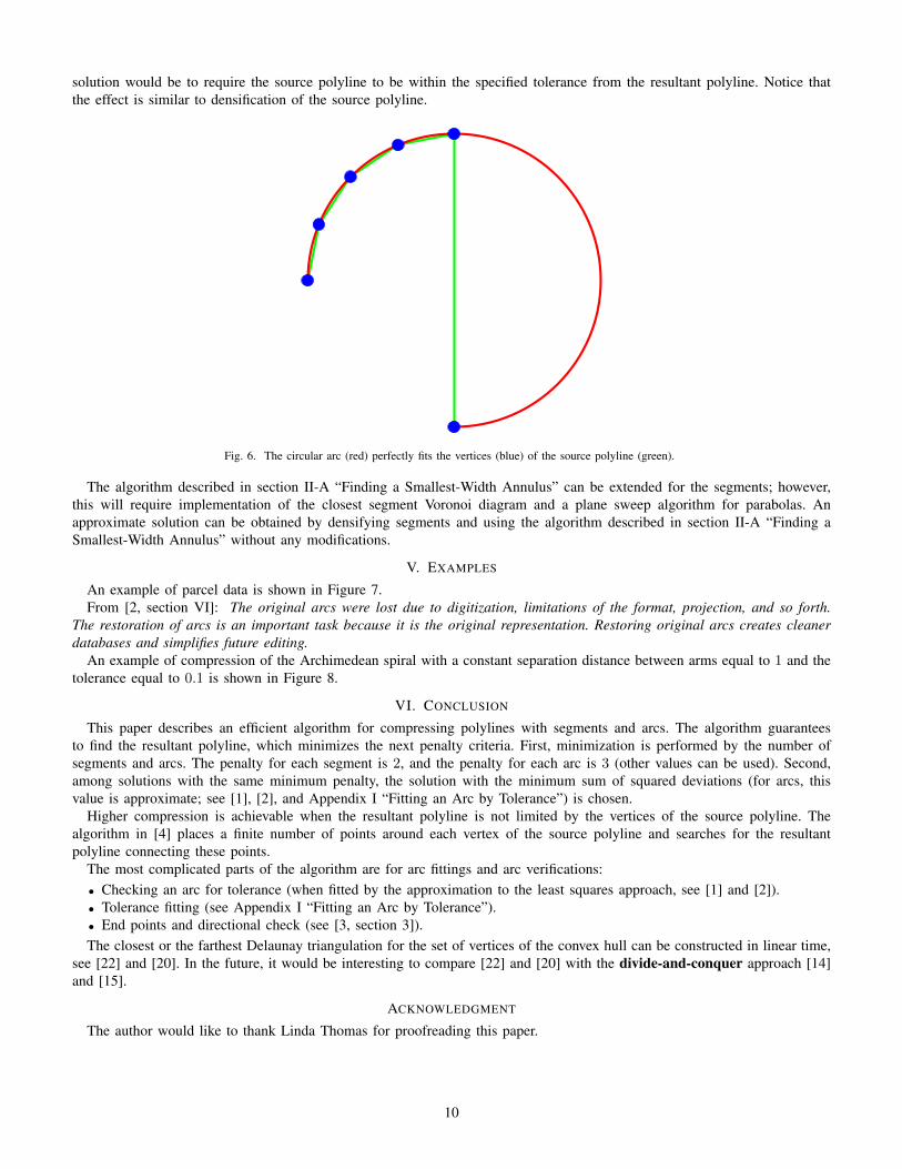
solution would be to require the source polyline to be within the specified tolerance from the resultant polyline. Notice thatthe effect is similar to densification of the source polyline.

Fig. 6. The circular arc (red) perfectly fits the vertices (blue) of the source polyline (green).

The algorithm described in section II-A “Finding a Smallest-Width Annulus” can be extended for the segments; however,this will require implementation of the closest segment Voronoi diagram and a plane sweep algorithm for parabolas. Anapproximate solution can be obtained by densifying segments and using the algorithm described in section II-A “Finding aSmallest-Width Annulus” without any modifications.

V. EXAMPLES

An example of parcel data is shown in Figure 7.From [2, section VI]: The original arcs were lost due to digitization, limitations of the format, projection, and so forth.

The restoration of arcs is an important task because it is the original representation. Restoring original arcs creates cleanerdatabases and simplifies future editing.

An example of compression of the Archimedean spiral with a constant separation distance between arms equal to 1 and thetolerance equal to 0.1 is shown in Figure 8.

VI. CONCLUSION

This paper describes an efficient algorithm for compressing polylines with segments and arcs. The algorithm guaranteesto find the resultant polyline, which minimizes the next penalty criteria. First, minimization is performed by the number ofsegments and arcs. The penalty for each segment is 2, and the penalty for each arc is 3 (other values can be used). Second,among solutions with the same minimum penalty, the solution with the minimum sum of squared deviations (for arcs, thisvalue is approximate; see [1], [2], and Appendix I “Fitting an Arc by Tolerance”) is chosen.

Higher compression is achievable when the resultant polyline is not limited by the vertices of the source polyline. Thealgorithm in [4] places a finite number of points around each vertex of the source polyline and searches for the resultantpolyline connecting these points.

The most complicated parts of the algorithm are for arc fittings and arc verifications:• Checking an arc for tolerance (when fitted by the approximation to the least squares approach, see [1] and [2]).• Tolerance fitting (see Appendix I “Fitting an Arc by Tolerance”).• End points and directional check (see [3, section 3]).The closest or the farthest Delaunay triangulation for the set of vertices of the convex hull can be constructed in linear time,

see [22] and [20]. In the future, it would be interesting to compare [22] and [20] with the divide-and-conquer approach [14]and [15].

ACKNOWLEDGMENT

The author would like to thank Linda Thomas for proofreading this paper.

10

Fig.

7.E

xam

ple

ofpa

rcel

data

.Sou

rce

poly

lines

are

show

nas

blac

klin

es.G

reen

poin

tsar

eth

eve

rtic

esof

the

sour

cepo

lylin

es.R

edpo

ints

are

the

vert

ices

ofth

ere

sulta

ntpo

lylin

es.

11

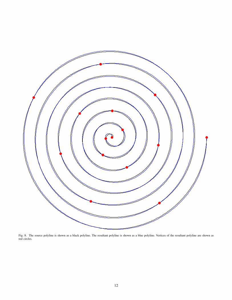
Fig. 8. The source polyline is shown as a black polyline. The resultant polyline is shown as a blue polyline. Vertices of the resultant polyline are shown asred circles.

12

APPENDIX I. FITTING AN ARC BY TOLERANCE

The center of an arc, passing through points A and B, should lie on the line that is equidistant from these points, seeFigure 9. The radius of the arc is the distance between its center and point A or B. Only if such an arc has its center lying onthe red-black-red line between the hyperbola branches (black part in yellow area) will point p be within the specified tolerancefrom the arc. Points that are no farther from A or B than the specified tolerance always satisfy the tolerance requirement.

A p

B

Fig. 9. The hyperbola for focal points A and p is shown as green and blue curved lines. The area between hyperbola branches is shown in yellow. The linethat is equidistant from A and B is shown as a red-black-red line.

Note that there is a possibility that the equidistant line will intersect only one hyperbola branch. In the case where theequidistant line intersects both hyperbola branches, two open intervals will satisfy the tolerance requirement. The number ofpossible intersections between a line and a hyperbola is 0, 1, and 2.

The intersection of all intervals constructed for all points will produce a set of intervals that satisfy the specified tolerance.The complexity of the algorithm is O(N log (N)), where N is the number of points; however, if we take into account thatthe most likely intervals are the one shown in Figure 9, then the complexity of the algorithm is O(N). This paper will onlyconsider worst-case complexity. If the set of intervals is empty, then no arc satisfies the specified tolerance; otherwise, of all

13

the possible solutions, the one that corresponds to an arc with the minimum approximate sum of squared deviations [2] istaken. Following are the steps of the algorithm for finding an arc within the specified tolerance:

1) Fit an arc when two points are known by the approximate solution of fitting an arc by the least squares approach [2].2) Check if this arc satisfies the tolerance requirement. If it does, then take it as the solution.3) Use the approach described in this appendix. If this algorithm does not find any solution (the set of intervals is empty),

then no arc can satisfy the specified tolerance.4) Evaluate the approximate sum of squared deviations for each end of the set of intervals found in step 3 for corresponding

arcs.5) Among the evaluated solutions, find one with the minimum value.In the case where the tolerance requirement should be satisfied for the source polyline segments, the solution is more

complicated; see the example in Figure 10. The yellow area is limited by the combination of hyperbolas and parabolas.

14

Fig. 10. The hyperbolas for focal point A and end points of the black segment are shown as green and blue lines. Parabolas equidistant from focal point Aand the black segment extended infinitely in both directions and shifted orthogonally in both directions by the specified tolerance are shown as red lines. Theline that is equidistant from A and B is shown as a dotted black line. The solution to where the center of an arc can be located (the dotted line inside theyellow area) passes through points A and B, while the black segment is within the specified tolerance from the arc.

15

APPENDIX II. EFFICIENT TOLERANCE CHECKING OF A SEGMENT

A test to determine if a segment from a start point to an end point has all vertices of the source polyline from i to j withinthe specified tolerance is performed by using the convex hull. The same test is performed for the end points to be withinthe tolerance, see [4, section II.C]. The number of possible combinations of indices i and j, i < j, is O

(N2), where N is

the number of vertices in the source polyline, and therefore the complexity to construct all convex hulls is O(N3 log (N)

).

However, not all of them are used. This paper will describe a different approach. Construct all convex hulls for subsets fromvertex k ·2q to vertex (k + 1) 2q−1, ∀k, q ∈ N0 and (k + 1) 2q ≤ N , see Figure 11. Note that it is possible to delay constructionof some of the convex hulls until they are needed. Complexity to construct all necessary convex hulls is O(N log (N)). Tocheck the segment for the tolerance requirement: First, convex hulls corresponding to the part of the source polyline fromvertex i to vertex j need to be found with the preferences for the longest; see the green cells in Figure 11. There is no needto merge convex hulls to perform a tolerance check. Second, the segment is tested against each convex hull. The complexityof one test is O

(log2 (K)

), where K is the number of vertices in the part of the source polyline.

0 1 2 3 4 5 6 7 8 9 10 11 12 13 14 15 16 17 18 19 200, 1 2, 3 4, 5 6, 7 8, 9 10, 11 12, 13 14, 15 16, 17 18, 19

0, 1, 2, 3 4, 5, 6, 7 8, 9, 10, 11 12, 13, 14, 15 16, 17, 18, 190, 1, 2, 3, 4, 5, 6, 7 8, 9, 10, 11, 12, 13, 14, 15

0, 1, 2, 3, 4, 5, 6, 7, 8, 9, 10, 11, 12, 13, 14, 15

Fig. 11. Each number represents an index of the vertex in the source polyline with N = 21 vertices. For each cell in the table, the convex hull is constructedfor the list of indices. This is done iteratively, with the first iteration constructing a convex hull for each pair of points, then at each successive iteration,merging each pair of convex hulls found in the previous iteration. Four green cells represent four convex hulls for the part of the source polyline from vertex 3to vertex 17.

16

APPENDIX III. TESTING PARTS OF THE SOURCE POLYLINE FOR ARC FITTING

Function Test, see Figure 12, will return a sorted list of parts of the source polyline that cannot be fitted with any arc withinthe specified tolerance. If the subset of points includes any of these parts, then it is not possible to fit an arc to this set ofpoints within the specified tolerance. For example, see the source polyline with N = 65 vertices in Figure 13 with the list of

pairs(

1017

),(

1219

),(

1421

),(

2633

),(

2835

),(

3037

),(

4249

),(

4451

), and

(4653

). Adding

(−10

)and

(N − 1N

)at the front and at

the end of this list correspondingly will make it simpler to use. This list is in the sorted order. Note that there are no pairscompletely inside any other pair. Therefore, in the list, both indices of the pairs are increasing.

function TESTfunction TESTPART(q, i, j)

if j < i? + 4 · 2q then returnend iffor i? from i while i? + 4 · 2q ≤ j step 2q do

j? = i? + 4 · 2q − 1if no arc within the specified tolerance can be fitted to Pi?,j? then

TESTPART(q + 1, i, j?)Report pair (i?, j?)i = i? + 2q

end ifend forTESTPART(q + 1, i, j)

end functionTESTPART(0, 0, N ) . N is the number of vertices in the source polyline

end function

Fig. 12. Function Test finds a sorted list of parts of the source polyline (pair of start and end indices) that cannot be fitted with any arc within the specifiedtolerance.

0

1

2

3

45

6

78

9

1011

12

13

14

15

16 17 18 19 20 21 22 23 24 25 26 27 28 29 30 31 32

33

34

35

3637 38

39 40 41 4243

44

45

46

47

48 49 50 51 52 53 54 55 5657 58

59 6061 62 63 64

Fig. 13. The red polyline with black vertices is the source polyline. The black vertices above are their indices. The green polyline is the optimal solution.

Determining if part of the source polyline Pi,j (all vertices from i to j) can be fitted with an arc within the specified tolerance

is performed by checking if pair(ij

)contains any pair from the sorted list of pairs. This is done by locating the position

of index i in the upper array a = (−1, 10, 12, 14, 26, 28, 30, 42, 44, 46, 64) (find the smallest qa satisfying i ≤ aqa ) and theposition of index j in the lower array b = (0, 17, 19, 21, 33, 35, 37, 49, 51, 53, 65) (find the smallest qb satisfying j < bqb ). If

qa < qb then pair(ij

)contains a pair from the list, and therefore, part of the source polyline Pi,j cannot be fitted with any

arc within the specified tolerance. This test is more than is needed in this paper.In order to reduce the number of combination in the dynamic search, it is necessary to find for index j the first index where

an arc can be fitted. This first index equals abj−1 + 1. If searching for the last index where an arc can be fitted for the indexi, the index is equal to bai − 1.

If, instead of the arrays a and b, the array with the first indices where an arc can be fitted for each index is prepared (0, 0,0, 0, 0, 0, 0, 0, 0, 0, 0, 0, 0, 0, 0, 0, 0, 11, 11, 13, 13, 15, 15, 15, 15, 15, 15, 15, 15, 15, 15, 15, 15, 27, 27, 29, 29, 31, 31,31, 31, 31, 31, 31, 31, 31, 31, 31, 31, 43, 43, 45, 45, 47, 47, 47, 47, 47, 47, 47, 47, 47, 47, 47, 47), then the binary searchcan be avoided. The complexity to create this array is O(N). For the last index, the array can also be prepared (16, 16, 16,16, 16, 16, 16, 16, 16, 16, 16, 18, 18, 20, 20, 32, 32, 32, 32, 32, 32, 32, 32, 32, 32, 32, 32, 34, 34, 36, 36, 48, 48, 48, 48,48, 48, 48, 48, 48, 48, 48, 48, 50, 50, 52, 52, 64, 64, 64, 64, 64, 64, 64, 64, 64, 64, 64, 64, 64, 64, 64, 64, 64, 64).

17

APPENDIX IV. DUALITY OF THE FARTHEST AND THE CLOSEST DELAUNAY DIAGRAMS BY INVERSIVE GEOMETRY

This appendix shows duality of the farthest Delaunay diagram with the closest Delaunay diagram by using inversive geometry[23]. The farthest Delaunay diagram only includes points on the convex hull. For some choice of the reference circle center,the closest Delaunay diagram constructed on an inverted set of points is dual to the farthest Delaunay diagram. This gives thepossibility to construct the farthest Delaunay diagram using algorithms for the closest Delaunay diagram.

The closest and the farthest Voronoi diagrams have opposite definitions. The closest Voronoi cell is a set of points closestto the same point. The farthest Voronoi cell is a set of points farthest from the same point. They are both dual to the closestand the farthest Delaunay diagrams, respectively. When there are no coincident points, they are both uniquely defined. Theclosest Voronoi diagram for each point has a cell; however, that is not the case for the farthest Voronoi diagram. Only pointsof the convex hull have cells. The link between the closest and the farthest Delaunay diagrams with the convex hull can beestablished by adding an extra dimension and by mapping each vertex to the paraboloid (x, y)→

(x, y, x2 + y2

)(see [13] and

[12]) or by inversion to sphere [21, section 6.3.2]. Therefore, the closest and the farthest Delaunay diagrams can be calculatedby constructing convex hull in higher dimensions.

This appendix establishes another link between the farthest and the closest Delaunay diagrams without adding an extradimension — by using inversive geometry in the same space. The link is from the farthest Delaunay diagram to the closestDelaunay diagram and is not unique. The farthest Delaunay diagram is dual to the closest Delaunay diagram for an invertedset of points inside an inverted convex hull. Therefore, all algorithms to construct the closest Delaunay diagram can be usedto construct the farthest Delaunay diagram.

A. Duality of the Farthest and the Closest Delaunay Diagrams

To establish duality between the farthest Delaunay diagram and the closest Delaunay diagram, the following definitions willbe used

• conv(S) is a set of vertices of the convex hull S.• CH(S) is a convex hull of S.• vol(P ) is an area of P .• Circles are represented as their borders.• Inside(c) is the area inside the circle c.• Outside(c) is the area outside the circle c.• CDC(S) is the set of closest Delaunay circles for the set of points S [12], i.e., satisfying that all points are outside or on

the border of each circle and each circle has points on the border forming nonempty geometry, {c|S ⊂ Outside(c) ∨ c∧ vol(CH(S ∩ c)) 6= 0}.

• FDC(S) is the set of farthest Delaunay circles for the set of points S [12], i.e., satisfying that all points are inside oron the border of each circle and each circle has points on the border forming nonempty geometry, {c|S ⊂ Inside(c) ∨ c∧ vol(CH(S ∩ c)) 6= 0}. This is the opposite of the definition of CDC(S).

Define circle inversion for a reference unit circle10 with center O

ΦO(x),

where x is an object or a set of objects that is inverted (point, circle, set of points, set of circles, etc.). The inverse of a pointp is equal to p′ =

p

‖p‖2, where ‖p‖ is Euclidean norm [23].

From inversive geometry theory [23], the circle inversion has the following properties:(a) ∀x, ∀O ⇒ ΦO(ΦO(x)) = x.(b) ∀ circle c,∀O /∈ c⇒ ΦO(c) is a circle.(c) ∀ circle c,∀O ∈ Inside(c)⇒ O ∈ Inside(ΦO(c)).(d) ∀ circle c, ∀O ∈ Outside(c)⇒ O ∈ Outside(ΦO(c)).(e) ∀ circle c, ∀O /∈ c ∧ ∀p ∈ c ⇒ p′ ∈ ΦO(c). For the circle containing O, the inverted points on the circle will maintain

their relative order and orientation. If O is outside of the circle, their relative order will be maintained but orientation willbe reversed.

(f ) ∀ circle c, ∀O ∈ Inside(c) ∧ ∀p ∈ Inside(c)⇒ ΦO(p) ∈ Outside(ΦO(c)).(g) ∀ circle c, ∀O ∈ Inside(c) ∧ ∀p ∈ Outside(c)⇒ ΦO(p) ∈ Inside(ΦO(c)).(h) ∀ circle c, ∀O ∈ Outside(c) ∧ ∀p ∈ Inside(c)⇒ ΦO(p) ∈ Inside(ΦO(c)).(i) ∀ circle c, ∀O ∈ Outside(c) ∧ ∀p ∈ Outside(c)⇒ ΦO(p) ∈ Outside(ΦO(c)).From the properties of inversive geometry and definitions of FDC(S) and CDC(S), it follows that

10Reference circles with the same center but having different radiuses are equivalent up to the scale.

18

X

Y

O

A

B

CD

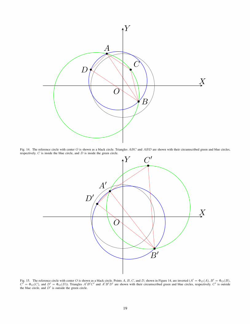
Fig. 14. The reference circle with center O is shown as a black circle. Triangles ABC and ABD are shown with their circumscribed green and blue circles,respectively. C is inside the blue circle, and D is inside the green circle.

X

Y

O

A′

B′

C ′

D′

Fig. 15. The reference circle with center O is shown as a black circle. Points A, B, C, and D, shown in Figure 14, are inverted (A′ = ΦO(A), B′ = ΦO(B),C′ = ΦO(C), and D′ = ΦO(D)). Triangles A′B′C′ and A′B′D′ are shown with their circumscribed green and blue circles, respectively. C′ is outsidethe blue circle, and D′ is outside the green circle.

19

(j) Any two triangles sharing the edge and satisfying the farthest or the closest Delaunay triangulation property (no pointsoutside or no points inside, respectively) and having circumscribed circles containing O will be inverted to nonoverlappingtriangles with opposite properties, see example in Figures 14 and 15. The proof follows from (e), (f ), and (g) that thepart of the circle on one side of AB containing C is inside the blue circle (see Figure 14) and will be inverted to thepart of the circle that is outside of the blue circle (see Figure 15). Therefore, the test to decide if point D lies inside thecircumscribed circle of A, B, and C is equivalent if point D′ lies outside of the circumscribed circle of A′, B′, and C ′.

X

Y

O

Fig. 16. The farthest Delaunay triangulation (green and blue lines) for the points (black points) of the convex hull. The convex hull border is shown as agreen polyline.

For the set of points S that are not on the line (otherwise, the Delaunay diagrams are trivial) this appendix will show theduality of the farthest Delaunay diagram with the closest Delaunay diagram by circle inversion. For any number of dimensions,the requirement is that the set of points S is not in the hyperplane; otherwise, the Delaunay diagram can be constructed in thehyperplane.(I) The farthest Voronoi diagram only includes points of the convex hull [12]. Therefore, S is a set of points that satisfy

S = conv(S) ∧ vol(CH(S)) 6= 0. From S = conv(S), it follows that S does not have any coincident and does not havemore than two collinear points.

(II) The convex hull of S is inside of all circles of the farthest Delaunay diagram with the exception that points of S areon the border of some circles. From the definition for the farthest Delaunay circles, stating that any circle of the farthestDelaunay diagram contains all points inside or on the border, it follows that any circle contains a convex hull of thesepoints, ∀c ∈ FDC(S)⇒ S ⊂ Inside(c) ∨ c⇒ CH(S) ⊂ Inside(c) ∨ c⇒ CH(S) \ S ⊂ Inside(c).

(III) Choose any point O inside or on the border of CH(S) but not a point from S, O ∈ CH(S) \ S.(IV) From (II) and (III), it follows that O is inside of all the circles of the farthest Delaunay diagram, ∀c ∈ FDC(S)⇒ O ∈

Inside(c). Because O is inside of all the circles of the farthest Delaunay diagram, from (c), it follows that O is insideof all inverted circles of the farthest Delaunay diagram, ∀c′ ∈ ΦO(FDC(S))⇒ O ∈ Inside(c′).

(V) Invert set of points S by unit circle with center O, S′ = ΦO(S).(VI) From (IV), (e), (f ), and definitions of FDC(S) and CDC(S), it follows that any inverted circle of the farthest Delaunay

diagram is also present in the closest Delaunay diagram, ΦO(FDC(S)) ⊂ CDC(S′).(VII) From (VI), and definitions of FDC(S) and CDC(S), it follows that ∀c′ ∈ CDC(S′) \ ΦO(FDC(S)) ⇒ O ∈

Outside(c′)∨c′. From the inversion of a circle that does not contain any point of S′ inside but has inversion center O inside,it follows that the inverted circle contains all the points of S inside or on the border. However, that circle is part of the far-thest Delaunay circles, which is a contradiction. Suppose O ∈ Inside(c′), then ΦO(c′) ∈ FDC(S)⇒ c′ ∈ ΦO(FDC(S)).Note that in two dimensions, O ∈ Outside(c′).

(VIII) From (IV), (VI), and (VII), it follows that ΦO({c′|CDC(S′) ∧O ∈ Inside(c′)}) = FDC(S).(IX) Inverted convex hull means the polygon connecting inverted convex hull vertices in the order of the original convex hull

vertices, see Figures 16 and 17.(X) From (e), (j), and (VIII), it follows that inversion of the farthest Delaunay diagram will be the closest Delaunay diagram

inside and on the border of the inverted convex hull. Note that this does not depend on the choice of point O in step (III);however, the closest Delaunay diagram outside of the inverted convex hull will depend on the choice of O, see two-dimensional example in Figures 16, 17, 18, and 19. Cases where more than n + 1 points are on the n dimensionalcircle of the Delaunay diagram correspond to nonunique Delaunay triangulation. These circles will have one-to-onecorrespondence in original and inverted spaces; therefore, the farthest and the closest Delaunay triangulations have aone-to-one relationship.

20

X

Y

O

Fig. 17. The closest Delaunay triangulation (green, blue, and red lines) for the inverted set of points (black points), see Figure 16. The inverted convex hullborder is shown as a green polyline. Red lines are outside of the inverted convex hull.

21

XY

O

Fig. 18. Same as Figure 17, with the difference that O is shifted to the border of the convex hull, see point O in the middle of the green segment. Theimage was resized to fit the page.

X

Y

O

Fig. 19. Inverted closest Delaunay triangulation (green and blue lines) for Delaunay circles containing O or inside of the inverted convex hull, see Figures 17or 18. This figure is exactly the same as Figure 16.

These statements prove the duality of the farthest Delaunay diagram with the closest Delaunay diagram in any number ofdimensions.

B. Properties of the Closest Delaunay Triangulation of Inverted Convex HullBecause points of the convex hull were inverted, the closest Delaunay triangulation of the inverted convex hull has the

following properties:• In two dimensions, for any triangulation of S′ that does not intersect the border of the inverted convex hull, for triangles

inside of the inverted convex hull, only one side is visible unless it contains point O, and for triangles outside of theinverted convex hull, two sides are visible from point O.

• In three dimensions, for any tetrahedration of S′ that does not intersect the border of the inverted convex hull, fortetrahedrons inside of the inverted convex hull, only one or two sides are visible unless it contains point O, and fortetrahedron outside of the inverted convex hull, two or three sides are visible from point O.

• In two dimensions, any triangulation inside the inverted convex hull will be inverted to the proper triangulation of theconvex hull.

C. Calculation of the Farthest Delaunay triangulation by the Closest Delaunay TriangulationFrom section “Duality of the Farthest and the Closest Delaunay Diagrams”, the farthest Delaunay triangulation can be

constructed from the closest Delaunay triangulation.11 The test to decide if point D′ lies inside the circumscribed circle of A′,B′, C ′, and D′ is evaluated by the sign of determinant∣∣∣∣∣∣∣∣

x′A y′A x′2A + y′2A 1x′B y′B x′2B + y′2B 1x′C y′C x′2C + y′2C 1x′D y′D x′2D + y′2D 1

∣∣∣∣∣∣∣∣ , (2)

where (x′, y′) = ΦO((x, y)) =

(x′ =

x

x2 + y2, y′ =

y

x2 + y2

)are inverted coordinates of A = (xA, yA), B = (xB , yB),

C = (xC , yC), and D = (xD, yD).

11If floating-point arithmetic is used, due to roundoff error the inverted convex hull might not correspond to the convex hull in the original space. In sucha case, the connection between the farthest Delaunay diagram and the closest Delaunay diagram might be broken.

22

Multiplying each row of (2) by x2A + y2A, x2B + y2B , x2C + y2C , and x2D + y2D, respectively, will not change the sign of thedeterminant (note that from (III), it follows that there are no points coincident with point O).∣∣∣∣∣∣∣∣

xA yA 1 x2A + y2AxB yB 1 x2B + y2BxC yC 1 x2C + y2CxD yD 1 x2D + y2D

∣∣∣∣∣∣∣∣ . (3)

Note that (3) is equal to minus ∣∣∣∣∣∣∣∣xA yA x2A + y2A 1xB yB x2B + y2B 1xC yC x2C + y2C 1xD yD x2D + y2D 1

∣∣∣∣∣∣∣∣ . (4)

Therefore, the test to decide if point D′ lies inside the circumscribed circle of A′, B′, C ′, and D′ can be performed in theoriginal space with the inversion of the sign of the determinant (4). Note that if coordinates of the points, in the original space,are integer numbers, then they will be represented in the inverted space as rational numbers.

D. Special Case where Points of the Convex Hull are Inverted to Points of the Convex Hull

From [23, chapter 7] (When Does Inversion Preserve Convexity?), there is a case where points of the convex hull can beinverted to the set of points of the convex hull. This happens when the intersection of the interiors of all circles constructed onneighboring vertices of the convex hull is not empty and the center of inversion is located in that intersection area. For sucha special set of points, it is possible to construct the closest Delaunay triangulation using the farthest Delaunay triangulation.

E. Remarks

This appendix shows the duality of the farthest Delaunay triangulation with the closest Delaunay triangulation by inversivegeometry. The choice of O is arbitrary, with the only requirement that it is inside of all farthest Delaunay hyperspheres. Thenew result of this appendix is that all algorithms for calculation of the closest Delaunay triangulation are also applicable tocalculation of the farthest Delaunay triangulation.

23

APPENDIX V. ALGORITHMS TO GENERATE RANDOM CONVEX HULLS

The ability to simulate a random convex hull is very important for testing and performance evaluation of differentimplementations for which the convex hull is an input. The distribution of the random convex hulls depends on the algorithmused to produce one. Therefore, several algorithms will be described in this appendix and, for three of them, examples willbe shown.

A. Random Set of Points

The algorithm is based on construction of a convex hull for a set of random points uniformly distributed in a square, acircle, or other shapes [24]. The main disadvantage of this algorithm is its tendency to reproduce a convex hull of the originalshape.

B. Random Distribution

This is similar to the algorithm described in the previous section, with the difference that the random points are distributedwith density having radial form [25], random walk, or other distributions [26]. From [26], the expected number of vertices inthe convex hull of a random walk of length n is approximately

2 log (n). (5)

Examples for convex hulls of random walks are shown in Figure 20.

C. Random Modifications of Edges

The algorithm is based on selecting randomly an edge and adding a vertex so that the new polygon is convex [27].

D. Random Modifications of Adjacent Edges

The algorithm is based on selecting randomly two neighboring edges of the convex hull, removing their common vertex,and randomly placing one point on each of them [28]. This approach has the property that, if it starts from any triangle, thenit cannot generate a square.

E. Random Set of Directions

This is a new approach to generate a convex hull from a random set of directions by simulating random weights to rescaledirections, which satisfies two restrictions:(a) The sum of squares of weights is equal to one.(b) The sum of weighted directions is equal to a vector of zero length.

The steps of the algorithm are as follows:1) Simulate n random unit vectors (xi, yi), i = 1, n. To simulate each random unit vector, the well-known solution is to

simulate a random angle α ∈ [−π, π) and obtain the unit vector as (cos (α), sin (α)). Another well-known solution is

to simulate two random variables (u, v) from uniform distribution in [−1, 1] and obtain the unit vector as(u, v)√u2 + v2

, if

u2 + v2 < 1 and u2 + v2 is not too small; otherwise, try again.2) Find orthogonal complement X of the subspace formed by two vectors (x1, x2, ..., xn) and (y1, y2, ..., yn), unless these

two vectors are close to collinear (absolute value of their correlation is close to one). In such a case, return to step 1.Matrix X has dimensions n× (n− 2) and satisfies

X> ·

x1 y1x2 y2...xn yn

= 0.

3) Generate random unit vector z of dimension n−2, z> ·z = 1. The well-known solution is to simulate a vector with n−2random variables from standard normal distribution and divide it by its length if the length is not too small; otherwise,try again.

4) Let w = X · z.Note that this satisfies conditions (a) and (b) because

w> · w = z> ·X> ·X · z =[X> ·X = I

]= z> · z = 1

and [x1 x2 · · · xny1 y2 · · · yn

]· w =

[x1 x2 · · · xny1 y2 · · · yn

]·X · z = 0 · z = 0.

24

Fig. 20. Examples of random convex hulls for a number of vertices in a random walk, 3, 7, 55, 2, 981, and 8, 886, 111, for each row from top to bottom.The number of vertices in a random walk is chosen so that in an approximate average, see (5), the expected number of vertices in the convex hull will be 2(a convex hull of three random points from a random walk will almost surely have three vertices), 4, 8, 16, and 32, correspondingly.

25

Resize all vectors (xi, yi) by wi,(xi, yi) = wi · (xi, yi) .

5) Sort all vectors (xi, yi), i = 1, n in a clockwise (or counterclockwise) direction12. Vectors of zero length can be ignored.6) Construct the convex hull:

Set p0 = (0, 0)For i = 1, n− 1

pi = pi−1 + (xi, yi)

Note that pn = pn−1 + (xn, yn) is approximately equal to p0 due to inexact floating-point arithmetic.The complexity of this algorithm is O(N log (N)). See examples of generated convex hulls in Figures 21, 22, and 23. While

this approach efficiently generates convex hulls with a large number of vertices, as the number of vertices increases, the shapeof the convex hull becomes more circular, see Figures 22 and 23.

F. From the Farthest Delaunay Triangulation

The algorithm described in this section is based on simulation of the farthest Delaunay triangulation [12]. Because thefarthest Delaunay triangulation only includes vertices of the convex hull, the result of the simulated triangulation is the convexhull. From the property of the farthest Delaunay triangulation that the circumscribed circle of each triangle contains all vertices,the simulation starts by generating a random segment on the unit circle, which cut the unit circle into two circular segments.Each consequent simulation consists of placing a point inside the circular segment, finding the circumscribed circle for thetriangle formed by the segment and the point, and replacing the circular segment with two new circular segments formed bythe end points of the segment and the point. This process guarantees that each iteration will not break the consistency of thefarthest Delaunay triangulation.

The steps of the algorithm are as follows:1) Generate two points on the unit circle. The segment connecting these two points divides the circle into two circular

segments. Put two circular segments into the list.2) Randomly select a circular segment from the list with probabilities proportional to the areas of circular segments.3) Simulate a random point inside the selected circular segment so that the distance from the point to the segment divided

by the height of the circular segment (this is similar to using the area of the triangle formed by the segment and therandom point) follows the Beta distribution. In this appendix, Beta distribution, with parameters (3, 1), was used, whichgives preference to a larger area.

4) Find the circumscribed circle for the ends of the segment and the simulated random point.5) Replace the selected circular segment with two circular segments between the end points of the segment and the simulated

point.The complexity of this algorithm is O(N log (N)). See examples of generated convex hulls in Figures 24, 25, and 26. Unlike

the algorithm described in section “Random Set of Directions”, there is no tendency to produce convex hulls like a circle, seeFigures 25 and 26; however, the circular segments tend to become too narrow. Practically, this algorithm will not be able togenerate convex hulls with more than a few hundred thousand vertices, as the new points will lie on the existing segments dueto the finite precision of floating-point arithmetic.

G. Remarks

Due to the use of rounded arithmetic, some of the generated vertices might not be vertices of the convex hull. Therefore,an additional step is needed to remove such vertices and obtain the final convex hull.

Let’s reiterate the importance of using different algorithms to generate a random convex hull to test and evaluate theperformance of different implementations for which the convex hull is an input. Using different algorithms to generate arandom convex hull will improve the quality of testing, as the algorithms will cover convex hulls with different properties:small angles, small segments, clustered vertices, etc..

12For example, using arctan2 (yi, xi) = −i log

xi + iyi√x2i + y2i

and requiring all angles to be in (−π, π].

26

Fig. 21. Examples of random convex hulls for a number of vertices, 3, 4, 5, 6, and 7, for each row from top to bottom.

27

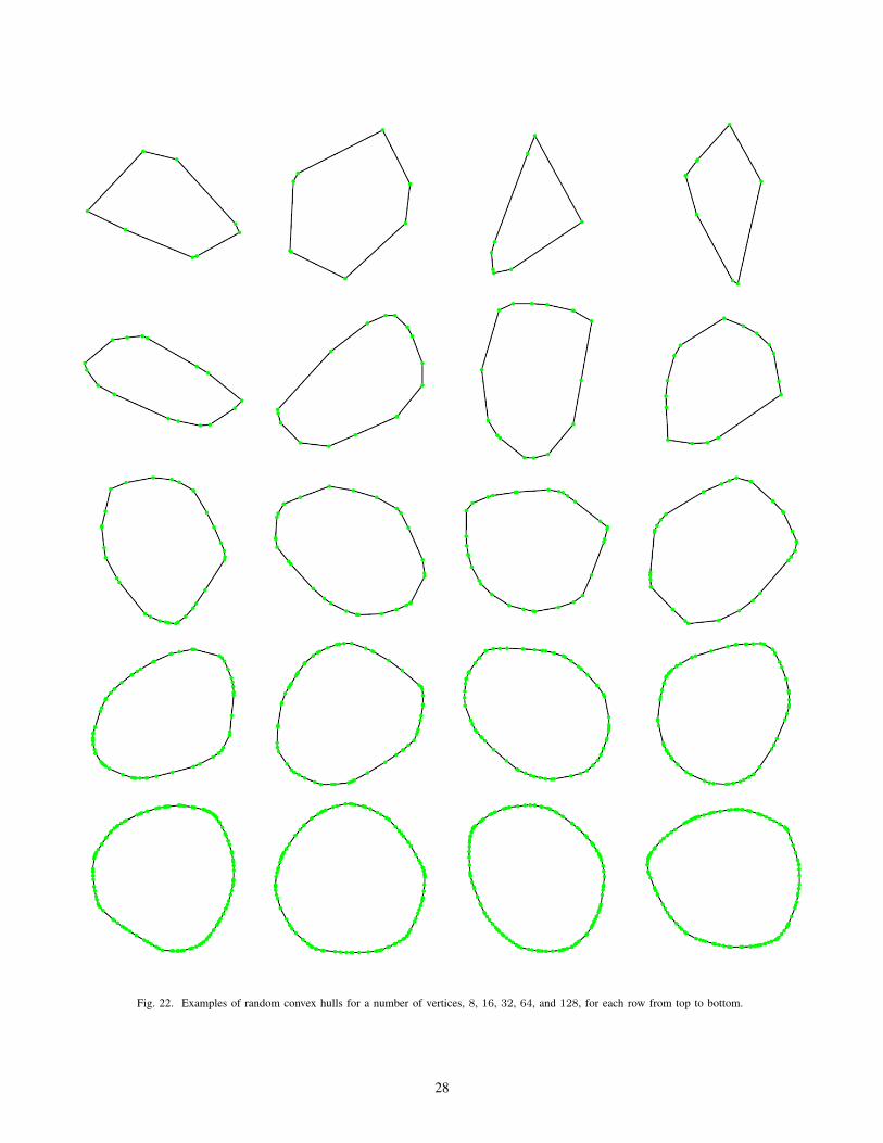
Fig. 22. Examples of random convex hulls for a number of vertices, 8, 16, 32, 64, and 128, for each row from top to bottom.

28

Fig. 23. Examples of random convex hulls for a number of vertices, 256, 512, 1, 024, 2, 048, and 4, 096, for each row from top to bottom.

29

Fig. 24. Examples of random convex hulls for a number of vertices, 3, 4, 5, 6, and 7, for each row from top to bottom.

30

Fig. 25. Examples of random convex hulls for a number of vertices, 8, 16, 32, 64, and 128, for each row from top to bottom.

31

Fig. 26. Examples of random convex hulls for a number of vertices, 256, 512, 1, 024, 2, 048, and 4, 096, for each row from top to bottom.

32

APPENDIX VI. CLIPPING SEGMENTS BY SQUARE

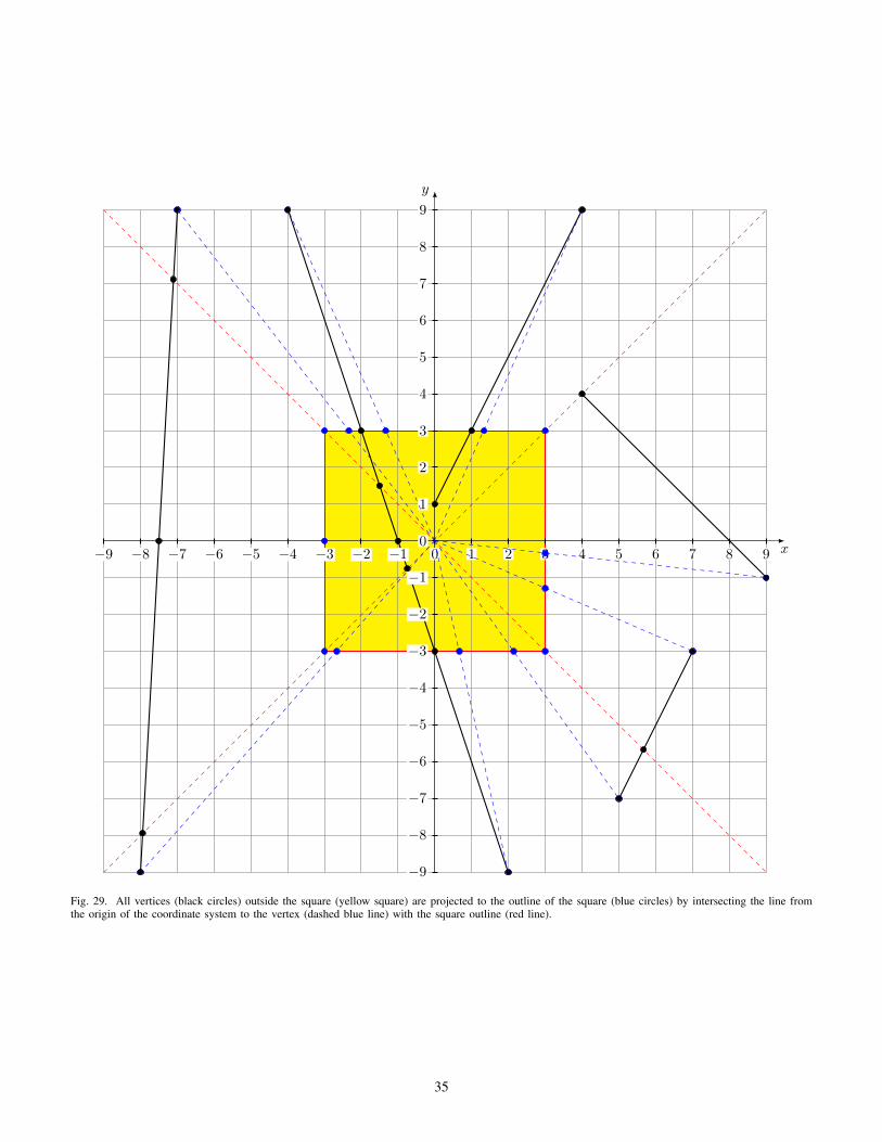
This section will describe a robust algorithm (proper despite inexact floating-point arithmetic) to clip all segments to a squarecentered at the origin of a coordinate system. Because all segments are part of some polygons, it is necessary to clip themin a way that preserves the topology of the polygons. The main ideas are to project points that are outside the square to thesquare outline by finding the intersection of the square outline and the line from the center of the coordinate system to theprojected point, and for all segments that have any part outside the square and are crossing any diagonal line, to divide themby the diagonal lines. Dividing segments by the diagonal lines solves inexact floating-point arithmetic issues and simplifiesthe algorithm to clip all segments by the square.

The area is divided into eight zones, see Figure 27.

X

Y

00

112233

44

55 66 77

Fig. 27. The division of a coordinate system into four areas (red, yellow, green, and blue) and four lines (black) with the exception of point (0, 0). They arenumbered counterclockwise from 0 to 7.

The algorithm to do robust clipping by square is as follows; see the examples shown in Figures 28, 29, and 30. For eachsegment in the list

1) If the segment does not have any points outside the square, return the segment.2) If the segment has one point in the origin of the coordinate system (0, 0), then return the intersection of this segment and

the square.3) If the points are in zones 0 and 4 or 2 and 6, the segment crosses two diagonal lines. Intersect this segment with OY or

OX axes, respectively (see red points in Figure 28), and add two segments to the list.4) If both points of the segment are in the odd zone, zones 1 and 5 or zones 3 and 7, then return the intersection of this

segment and the square.5) If the segment is crossing a diagonal line, then divide it by the diagonal line and add both segments to the list.6) Both points of the segment are in the even zone extended by the zone’s border (see red, yellow, green, or blue areas in

Figure 27). If there are no points inside the square (excluding the square outline), project both points to the square outline(see Figure 29) and return the resultant segment.

7) Both points of the segment are in the even zone extended by the zone’s border; one of the points is inside the square, andanother is outside. Therefore, the segment intersects the outline of the square only at one point. Divide this segment bythe intersection point. The intersection point must be in the same zone extended by the zone’s border. If the intersectionpoint falls within another zone due to inexact calculations, it has to be adjusted. Add the segment that is outside thesquare to the list (process it by step 6) and return the segment that is inside the square.

The result of performing this algorithm is shown in Figure 30.

33

x

y

−9 −8 −7 −6 −5 −4 −3 −2 −1 0 1 2 3 4 5 6 7 8 9

−9

−8

−7

−6

−5

−4

−3

−2

−1

0

1

2

3

4

5

6

7

8

9

Fig. 28. Examples of segments are shown as black lines having ends with black circles. The points where they intersect the coordinate system axis areshown as red circles. The points where segments intersect diagonal lines (dashed red lines) are shown as green circles. The points where segments intersectthe square outline are shown as blue circles.

34

x

y

−9 −8 −7 −6 −5 −4 −3 −2 −1 0 1 2 3 4 5 6 7 8 9

−9

−8

−7

−6

−5

−4

−3

−2

−1

0

1

2

3

4

5

6

7

8

9

Fig. 29. All vertices (black circles) outside the square (yellow square) are projected to the outline of the square (blue circles) by intersecting the line fromthe origin of the coordinate system to the vertex (dashed blue line) with the square outline (red line).

35

x

y

−4 −3 −2 −1 0 1 2 3 4

−4

−3

−2

−1

0

1

2

3

4

Fig. 30. The result of clipping all the segments (shown in Figure 28) by the square.

36

APPENDIX VII. ALGORITHM TO REMOVE OVERLAPPING SEGMENTS

All segments are specified with integer coordinates. Each segment has a list of indices. The indices of each segment areindices of the polygons for which the segment is a border segment. The next algorithm will detect all overlapping segments.In some parts of the algorithm, it would be necessary to merge lists of indices. This operation applies the “XOR” rule, whichmeans that only indices occurring an odd number of times in both lists will be present in the final list, but only once.

1) Discard segments of zero length.2) Assign each segment an integer vector: (

xy

)=

(x1y1

)−(x0y0

)gcd (x1 − x0, y1 − y0)

,

where(x0y0

)and

(x1y1

)are starting and ending vertices of the segment, and gcd is the greatest common divisor.

Make adjustments for opposite directions

(xy

)=

−(xy

), if x < 0 ∨ x = 0 ∧ y < 0,(

xy

), otherwise.

3) Using a hash table or sorting all integer vectors, group all segments having the same integer vector.

4) For each group of segments sharing an integer vector(xy

)a) Assign each segment an integer value equal to the vector product of the integer vector to any end point of the segment

(the result is the same because the integer vector is parallel to the segment).13

b) Using a hash table or sorting all integer values, group all segments having the same integer value.c) For each group of segments sharing an integer value

i) Put all end points of segments with the list of indices into an array. Each element of the array is a pair of a pointand a list of indices.

ii) Sort this array by x-coordinate if the x-coordinates are different; otherwise, sort them by y-coordinate.iii) Merge elements of the array with equal points by merging their lists of indices.iv) Remove elements of the array with an empty list of indices.v) For each element in the array, merge indices with indices of the previous element from beginning to end (the last

element should have an empty list of indices).vi) For each element in the array with a nonempty list of indices, create a segment starting with the element point,

ending with the next element point, and having indices of that element.This algorithm creates a new list of segments without any overlaps.

13This operation will approximately double the number of bits and might require the use of extended precision.

37

APPENDIX VIII. EFFICIENT EXTRACTION OF ELEMENTS IN SORTED ORDER FROM ANY SUBARRAY

Efficient extraction of elements in sorted order from any subarray is performed by preprocessing the array using a methodvery similar to mergesort [29, chapter 5], see Figure 31. The only difference is that the previous step of the mergesortalgorithm is kept in memory. The complexity of this step is the same as the complexity of mergesort, which is O(N log (N)),where N is the number of elements in the array. Then, extraction of elements in sorted order from any subarray is performedby finding corresponding sorted arrays with the preferences for the longest (see the green cells in Figure 31) and merging,starting with the shortest (similar to steps of the mergesort algorithm). Because there are no more than two sorted arrays foreach size of 2i, i ∈ N0∧2i ≤ K, where K is the number of elements in the subarray, the complexity of merging sorted arraysis O(K); however, not all elements are needed. To extract a few elements in sorted order, put all sorted arrays in the treestructure, starting with the shortest, and rearrange them to make all child nodes of the tree no smaller than their parent nodes,as shown in Figure 32. This is similar to merging of leftist trees [30, part 5]. The complexity of this step is O(log (K)). Thisforms a priority tree with some nodes referring to the position in the sorted arrays shown in green in Figures 31, 32, 33, and34. Modifications of the tree with the first and second elements removed are shown in Figures 33 and 34. While the worst-casecomplexity of each request to remove the minimum element is O(log (K)), the total complexity to extract all elements of thesubarray in sorted order is still O(K). Therefore, the amortized time complexity to remove an element is O(1).

8 5 13 16 6 1 14 3 15 4 17 0 12 10 19 7 20 10 18 11 95, 8 13, 16 1, 6 3, 14 4, 15 0, 17 10, 12 7, 19 10, 20 11, 18

5, 8, 13, 16 1, 3, 6, 14 0, 4, 15, 17 7, 10, 12, 19 10, 11, 18, 201, 3, 5, 6, 8, 13, 14, 16 0, 4, 7, 10, 12, 15, 17, 19

0, 1, 3, 4, 5, 6, 7, 8, 10, 12, 13, 14, 15, 16, 17, 19

Fig. 31. The first row is the array of size N = 21. Each element of the next row groups two elements of the previous row and sorts all elements in them(similar to a step of the mergesort algorithm). The process is continued for all rows until there is nothing left to group. In the result, any subarray can berepresented as several sorted arrays (green cells for the subarray of size K = 18). Note that it is possible to delay construction of the sorted arrays until theyare needed.

0

0, 4, 7, 10, 12, 15, 17, 191

1, 3, 6, 145

10, 2013

13, 1618

Fig. 32. Priority queue based on the tree with all child nodes no smaller than their parent nodes (changes are shown in red).

Note that in a dynamic programming approach, see step 2 in section III “Dynamic Programming”, elements of the array areadded one by one.

38

1

0, 4, 7, 10, 12, 15, 17, 193

1, 3, 6, 145

10, 2013

13, 1618

Fig. 33. Modified priority queue after removing the first element (changes are shown in red).

3

0, 4, 7, 10, 12, 15, 17, 195

1, 3, 6, 1410

10, 2013

13, 1618

Fig. 34. Modified priority queue after removing the second element (changes are shown in red).

39

REFERENCES

[1] L. Dorst, “Total least squares fitting of k-spheres in n-d Euclidean space using an (n+2)-d isometric representation,” Journal of Mathematical Imagingand Vision, vol. 50, no. 3, pp. 214–234, 2014. [Online]. Available: http://doi.org/10.1007/s10851-014-0495-2

[2] A. Gribov, “Approximate fitting of circular arcs with complexity O(1),” ArXiv e-prints, May 2015. [Online]. Available: http://arxiv.org/abs/1504.06582[3] E. Bodansky and A. Gribov, “Approximation of polylines with circular arcs,” in Graphics Recognition. Recent Advances and Perspectives, ser.

Lecture Notes in Computer Science, J. Llados and Y.-B. Kwon, Eds. Springer Berlin Heidelberg, 2004, vol. 3088, pp. 193–198. [Online]. Available:http://doi.org/10.1007/978-3-540-25977-0 18

[4] A. Gribov, “Searching for a compressed polyline with a minimum number of vertices,” ArXiv e-prints, April 2015. [Online]. Available:http://arxiv.org/abs/1504.06584

[5] W. S. Chan and F. Chin, “Approximation of polygonal curves with minimum number of line segments or minimum error,” International Journal ofComputational Geometry & Applications, vol. 06, no. 01, pp. 59–77, 1996. [Online]. Available: http://dx.doi.org/10.1142/S0218195996000058

[6] A. Safonova and J. Rossignac, “Compressed piecewise-circular approximations of 3D curves,” Computer-Aided Design, vol. 35, pp. 533–547, May2003. [Online]. Available: http://dx.doi.org/10.1016/S0010-4485(02)00073-8

[7] R. S. Drysdale, G. Rote, and A. Sturm, “Approximation of an open polygonal curve with a minimum number of circular arcs and biarcs,” ComputationalGeometry: Theory and Applications, vol. 41, no. 1-2, pp. 31–47, October 2008. [Online]. Available: http://doi.org/10.1016/j.comgeo.2007.10.009

[8] A. Gribov and E. Bodansky, “A new method of polyline approximation,” in Structural, Syntactic, and Statistical Pattern Recognition, ser. LectureNotes in Computer Science, A. Fred, T. M. Caelli, R. P. Duin, A. Campilho, and D. de Ridder, Eds. Springer Berlin Heidelberg, 2004, vol. 3138, pp.504–511. [Online]. Available: http://dx.doi.org/10.1007/978-3-540-27868-9 54

[9] L. Yin, Y. Yajie, and L. Wenyin, “Online segmentation of freehand stroke by dynamic programming,” in Eighth International Conference on DocumentAnalysis and Recognition, vol. 1, August 2005, pp. 197–201. [Online]. Available: http://doi.org/10.1109/ICDAR.2005.180

[10] A. Gribov and E. Bodansky, “Reconstruction of orthogonal polygonal lines,” in Document Analysis Systems VII, ser. Lecture Notes in Computer Science,H. Bunke and A. Spitz, Eds. Springer Berlin Heidelberg, 2006, vol. 3872, pp. 462–473. [Online]. Available: http://dx.doi.org/10.1007/11669487 41

[11] J. Hershberger and J. Snoeyink, “Speeding up the Douglas-Peucker line-simplification algorithm,” in Proceedings of the 5th International Symposiumon Spatial Data Handling, 1992, pp. 134–143.

[12] M. de Berg, O. Cheong, M. van Kreveld, and M. Overmars, Computational Geometry: Algorithms and Applications, 3rd ed. Santa Clara, CA, USA:Springer-Verlag TELOS, 2008.

[13] D. Eppstein, “The farthest point Delaunay triangulation minimizes angles,” Computational Geometry, vol. 1, no. 3, pp. 143–148, 1992. [Online].Available: http://doi.org/10.1016/0925-7721(92)90013-I

[14] D. T. Lee and B. J. Schachter, “Two algorithms for constructing a Delaunay triangulation,” International Journal of Computer & Information Sciences,vol. 9, no. 3, pp. 219–242, 1980. [Online]. Available: http://doi.org/10.1007/BF00977785

[15] L. Guibas and J. Stolfi, “Primitives for the manipulation of general subdivisions and the computation of Voronoi,” ACM Trans. Graph., vol. 4, no. 2,pp. 74–123, April 1985. [Online]. Available: http://doi.org/10.1145/282918.282923

[16] R. A. Dwyer, “A faster divide-and-conquer algorithm for constructing Delaunay triangulations,” Algorithmica, vol. 2, no. 1, pp. 137–151, 1987.[Online]. Available: http://doi.org/10.1007/BF01840356

[17] S. Fortune, Voronoi diagrams and Delaunay triangulations, 2nd ed. World Scientific, 1995, vol. 4, pp. 225–265. [Online]. Available:http://doi.org/10.1142/9789812831699 0007

[18] T. H. Cormen, C. E. Leiserson, R. L. Rivest, and C. Stein, Introduction to Algorithms, 3rd ed. The MIT Press, 2009.[19] S. Fortune, “A note on Delaunay diagonal flips,” Pattern Recogn. Lett., vol. 14, no. 9, pp. 723–726, September 1993. [Online]. Available:

http://doi.org/10.1016/0167-8655(93)90142-Z[20] H. N. Djidjev and A. Lingas, “On computing Voronoi diagrams for sorted point sets,” International Journal of Computational Geometry & Applications,

vol. 05, no. 03, pp. 327–337, 1995. [Online]. Available: http://doi.org/10.1142/S0218195995000192[21] F. P. Preparata and M. I. Shamos, Computational Geometry: An Introduction. New York, NY, USA: Springer-Verlag New York, Inc., 1985.[22] A. Aggarwal, L. J. Guibas, J. Saxe, and P. W. Shor, “A linear-time algorithm for computing the Voronoi diagram of a convex polygon,” Discrete &

Computational Geometry, vol. 4, no. 6, pp. 591–604, 1989. [Online]. Available: http://doi.org/10.1007/BF02187749[23] D. E. Blair, Inversion Theory and Conformal Mapping, ser. Student Mathematical Library. American Mathematical Society, 2000, vol. 9.[24] S. Har-Peled, “On the expected complexity of random convex hulls,” CoRR, vol. abs/1111.5340, December 2011. [Online]. Available:

http://arxiv.org/abs/1111.5340[25] L. Devroye, “On the computer generation of random convex hulls,” Computers & Mathematics with Applications, vol. 8, no. 1, pp. 1–13, 1982.

[Online]. Available: http://doi.org/10.1016/0898-1221(82)90035-9[26] S. N. Majumdar, A. Comtet, and J. Randon-Furling, “Random convex hulls and extreme value statistics,” Journal of Statistical Physics, vol. 138, no. 6,

pp. 955–1009, 2010. [Online]. Available: http://doi.org/10.1007/s10955-009-9905-z[27] S. A. Kryukov, “Solution 1 (Algorithm for random polygon generation),” September 2013. [Online]. Available: http://www.codeproject.com/Answers/

651591/algorithm-for-random-polygon-generation#answer1[28] ——, “Solution 2 (Algorithm for random polygon generation),” September 2013. [Online]. Available: http://www.codeproject.com/Answers/652131/

algorithm-for-random-polygon-generation#answer2[29] D. E. Knuth, The Art of Computer Programming: Sorting and Searching, 2nd ed. Redwood City, CA, USA: Addison Wesley Longman Publishing Co.,

Inc., 1998, vol. 3.[30] D. P. Mehta and S. Sahni, Handbook of Data Structures and Applications (Chapman & Hall/CRC Computer and Information Science Series). Chapman

& Hall/CRC, 2004.

40