optimal and simple monetary policy rules with zero floor on the nominal interest rate

Optimal and Simple Monetary Policy Ruleswith Zero Floor on the Nominal Interest Rate∗

Anton NakovBanco de Espana

Recent treatments of the issue of a zero floor on nominalinterest rates have been subject to some important method-ological limitations. These include the assumption of perfectforesight or the introduction of the zero lower bound as aninitial condition or a constraint on the variance of the inter-est rate, rather than an occasionally binding non-negativityconstraint. This paper addresses these issues, offering a globalsolution to a standard dynamic stochastic sticky-price modelwith an explicit occasionally binding non-negativity constrainton the nominal interest rate. It turns out that the dynam-ics and sometimes the unconditional means of the nominalrate, inflation, and the output gap are strongly affected byuncertainty in the presence of the zero lower bound. Commit-ment to the optimal rule reduces unconditional welfare lossesto around one-tenth of those achievable under discretionarypolicy, while constant price-level targeting delivers losses thatare only 60 percent larger than those under the optimal rule.Even though the unconditional performance of simple instru-ment rules is almost unaffected by the presence of the zerolower bound, conditional on a strong deflationary shock, simpleinstrument rules perform substantially worse than the optimalpolicy.

JEL Codes: E31, E32, E37, E47, E52.

∗I would like to thank Kosuke Aoki, Fabio Canova, Wouter den Haan, JordiGalı, Albert Marcet, Ramon Marimon, Bruce Preston, Morten Ravn, MichaelReiter, Thijs van Rens, John Taylor, and an anonymous referee for helpful com-ments and suggestions. I am grateful also for comments to seminar participantsat Universitat Pompeu Fabra, ECB, Banco de Espana, Central European Univer-sity, Warwick University, Mannheim University, New Economic School, Rutgers

73

74 International Journal of Central Banking June 2008

1. Introduction

An economy is said to be in a “liquidity trap” when the mone-tary authority cannot achieve a lower nominal interest rate in orderto stimulate output. Such a situation can arise when the nominalinterest rate has reached its zero lower bound (ZLB), below whichnobody would be willing to lend, if money can be stored at no costfor a nominally riskless zero rate of return.

The possibility of a liquidity trap was first suggested by Keynes(1936) with reference to the Great Depression of the 1930s. At thattime he compared the effectiveness of monetary policy in such asituation to trying to “push on a string.” After WWII and espe-cially during the high-inflation period of the 1970s, interest in thetopic receded, and the liquidity trap was relegated to a hypotheticaltextbook example. As Krugman (1998) noticed, of the few modernpapers that dealt with it, most concluded that “the liquidity trapcan’t happen, it didn’t happen, and it won’t happen again.”

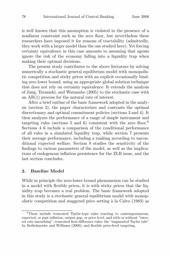
With the benefit of hindsight, however, it did happen, and tono less than Japan. Figure 1 illustrates this, showing the evolutionof output, inflation, and the short-term nominal interest rate fol-lowing the collapse of the Japanese real estate bubble of the late1980s. The figure exhibits a persistent downward trend in all threevariables and, in particular, the emergence of deflation since 1998coupled with a zero nominal interest rate since 1999.

Motivated by the recent experience of Japan, the aim of thepresent paper is to contribute a quantitative analysis of the ZLBissue in a standard sticky-price model under alternative monetarypolicy regimes. On the one hand, the paper characterizes optimalmonetary policy in the case of discretion and commitment.1 Onthe other hand, it studies the performance of several simple mone-tary policy rules, modified to comply with the zero floor, relative tothe optimal commitment policy. The analysis is carried out within

University, HEC Montreal, EBRD, Koc University, and Universidad de Navarra.Financial support from the Spanish Ministry of Foreign Affairs (Becas MAE) andthe ECB are gratefully acknowledged.

1The part of the paper on optimal policy is similar to independent work byAdam and Billi (2006, 2007). The added value is to quantify and compare theperformance of optimal commitment policy with that of a number of suboptimalrules in the same stochastic sticky-price setup.

Vol. 4 No. 2 Optimal and Simple Monetary Policy Rules 75

Figure 1. Japan’s Fall into a Liquidity Trap

a stochastic general equilibrium model with monopolistic compe-tition and Calvo (1983) staggered price setting, under a standardcalibration to the postwar U.S. economy.

The main findings are as follows: the optimal discretionary policywith zero floor involves a deflationary bias, which may be significantfor certain parameter values and which implies that any quantitativeanalyses of discretionary biases of monetary policy that ignore thezero lower bound may be misleading. In addition, optimal discre-tionary policy implies much more aggressive cutting of the interestrate when the risk of deflation is high, compared with the corre-sponding policy without zero floor. Such a policy helps mitigate thedepressing effect of private-sector expectations on current outputand prices when the probability of falling into a liquidity trap ishigh.2

2An early version of this paper comparing the performance of optimal dis-cretionary policy with three simple Taylor rules was circulated in 2004; optimalcommitment policy and more simple rules were added in a version circulated in2005. Optimal discretionary policy was studied independently by Adam and Billi(2004b), and optimal commitment policy by Adam and Billi (2004a).


In contrast, optimal commitment policy involves less preemptivelowering of the interest rate in anticipation of a liquidity trap, butit entails a promise for sustained monetary policy easing followingan exit from a trap. This type of commitment enables the centralbank to achieve higher expected (and actual) inflation and lower realrates in periods when the zero floor on nominal rates is binding.3

As a result, under the baseline calibration, the expected welfare lossunder commitment is only around one-tenth of the loss under opti-mal discretionary policy. This implies that the cost of discretion maybe much higher than normally considered when abstracting from thezero-lower-bound issue.

The average welfare losses under simple instrument rules areeight to twenty times larger than those under the optimal rule. How-ever, the bulk of these losses stem from the intrinsic suboptimalityof simple instrument rules and not from the zero floor per se. Thisis related to the fact that under these rules the zero floor is hitvery rarely—less than 1 percent of the time—compared with opti-mal commitment policy, which visits the liquidity trap one-third ofthe time. On the other hand, conditional on a large deflationaryshock, the relative performance of simple instrument rules deterio-rates substantially vis-a-vis the optimal commitment policy.

Issues of deflation and the liquidity trap have received consid-erable attention recently, especially after the experience of Japan.4

In an influential article, Krugman (1998) argued that the liquid-ity trap boils down to a credibility problem in which private agentsexpect any monetary expansion to be reverted once the economy hasrecovered. As a solution, he suggested that the central bank shouldcommit to a policy of high future inflation over an extended horizon.

More recently, Jung, Teranishi, and Watanabe (2005) haveexplored the effect of the zero lower bound in a standard sticky-pricemodel with Calvo price setting under the assumption of perfect fore-sight. Consistent with Krugman (1998), they conclude that optimal

3This basic intuition was suggested already by Krugman (1998), based on asimpler model.

4A partial list of relevant studies includes Krugman (1998), Wolman (1998),McCallum (2000), Reifschneider and Williams (2000), Eggertsson and Woodford(2003), Klaeffling and Lopez-Perez (2003), Coenen, Orphanides, and Wieland(2004), Jung, Teranishi, and Watanabe (2005), Kato and Nishiyama (2005), andAdam and Billi (2006, 2007).


commitment policy entails a promise of a zero nominal interest forsome time after the economy has recovered. Eggertsson and Wood-ford (2003) study optimal commitment policy with zero lower boundin a similar model in which the natural rate of interest is allowedto take two different values. In particular, it is assumed to becomenegative initially and then to jump to its “normal” positive levelwith a fixed probability in each period. These authors also concludethat the central bank should create inflationary expectations for thefuture. Importantly, they derive a moving price-level targeting rulethat delivers the optimal commitment policy in this model.

One shortcoming of much of the modern literature on monetarypolicy rules is that it largely ignores the ZLB issue or at best usesrough approximations to address the problem. For instance, Rotem-berg and Woodford (1997) introduce nominal rate targeting as anadditional central bank objective, which ensures that the resultingpath of the nominal rate does not violate the zero lower bound toooften. In a similar vein, Schmitt-Grohe and Uribe (2004) excludefrom their analysis instrument rules that result in a nominal ratewith an average that is less than twice its standard deviation. Inboth cases, therefore, one might argue that for sufficiently largeshocks that happen with a probability as high as 5 percent, thederived monetary policy rules are inconsistent with the zero lowerbound.

On the other hand, of the few papers that do introduce an explicitnon-negativity constraint on nominal interest rates, most simplifythe stochastics of the model—e.g., by assuming perfect foresight(Jung, Teranishi, and Watanabe 2005) or a two-state low/high econ-omy (Wolman 1998; Eggertsson and Woodford 2003). Even then, thezero lower bound is effectively imposed as an initial (“low”) conditionand not as an occasionally binding constraint.5 While this assump-tion may provide a reasonable first pass at a quantitative analysis,it may be misleading to the extent that it ignores the occasionallybinding nature of the zero interest rate floor.

Other studies (e.g., Coenen, Orphanides, and Wieland 2004) layout a stochastic model but knowingly apply inappropriate solutiontechniques that rely on the assumption of certainty equivalence. It

5Namely, the zero floor binds for the first several periods, but once the econ-omy transits to the “high” state, the ZLB never binds thereafter.


is well known that this assumption is violated in the presence of anonlinear constraint such as the zero floor, but nevertheless theseresearchers have imposed it for reasons of tractability (admittedly,they work with a larger model than the one studied here). Yet forcingcertainty equivalence in this case amounts to assuming that agentsignore the risk of the economy falling into a liquidity trap whenmaking their optimal decisions.

The present study contributes to the above literature by solvingnumerically a stochastic general equilibrium model with monopolis-tic competition and sticky prices with an explicit occasionally bind-ing zero lower bound, using an appropriate global solution techniquethat does not rely on certainty equivalence. It extends the analysisof Jung, Teranishi, and Watanabe (2005) to the stochastic case withan AR(1) process for the natural rate of interest.

After a brief outline of the basic framework adopted in the analy-sis (section 2), the paper characterizes and contrasts the optimaldiscretionary and optimal commitment policies (sections 3 and 4). Itthen analyzes the performance of a range of simple instrument andtargeting rules (sections 5 and 6) consistent with the zero floor.6

Sections 4–6 include a comparison of the conditional performanceof all rules in a simulated liquidity trap, while section 7 presentstheir average performance, including a ranking according to uncon-ditional expected welfare. Section 8 studies the sensitivity of thefindings to various parameters of the model, as well as the implica-tions of endogenous inflation persistence for the ZLB issue, and thelast section concludes.

2. Baseline Model

While in principle the zero-lower-bound phenomenon can be studiedin a model with flexible prices, it is with sticky prices that the liq-uidity trap becomes a real problem. The basic framework adoptedin this study is a stochastic general equilibrium model with monop-olistic competition and staggered price setting a la Calvo (1983) as

6These include truncated Taylor-type rules reacting to contemporaneous,expected, or past inflation, output gap, or price level, and with or without “inter-est rate smoothing”; truncated first-difference rules; the “augmented Taylor rule”by Reifschneider and Williams (2000); and flexible price-level targeting.


in Galı (2003) and Woodford (2003). In its simplest log-linearizedversion,7 the model consists of three building blocks, describing thebehavior of households, firms, and the monetary authority.

The first block, known as the “IS curve,” summarizes the house-hold’s optimal consumption decision,

xt = Etxt+1 − σ(it − Etπt+1 − rn

t

). (1)

It relates the “output gap” xt (i.e., the deviation of output fromits flexible-price equilibrium) positively to the expected future out-put gap and negatively to the gap between the ex ante real interestrate, it − Etπt+1, and the “natural” (i.e., flexible-price equilibrium)real rate, rn

t (which is observed by all agents at time t). Consump-tion smoothing accounts for the positive dependence of current out-put demand on expected future output demand, while intertemporalsubstitution implies the negative effect of the ex ante real interestrate. The interest rate elasticity of output, σ, corresponds to theinverse of the coefficient of relative risk aversion in the consumers’utility function.

The second building block of the model is a “Phillips curve”-type equation, which derives from the optimal price-setting deci-sion of monopolistically competitive firms under the assumption ofstaggered price setting a la Calvo (1983),

πt = βEtπt+1 + κxt, (2)

where β is the time discount factor and κ, the “slope” of the Phillipscurve, is related inversely to the degree of price stickiness.8 Sincefirms are unable to adjust prices optimally every period, whenever

7It is important to note that, like in the studies cited in the introduction,the objective here is a modest one, in that the only source of nonlinearity inthe model stems from the ZLB. Solving the fully nonlinear sticky-price modelwith Calvo (1983) contracts can be a worthwile enterprise; however, it increasesthe dimensionality of the computational problem by the number of states andco-states that one should keep track of (e.g., the measure of price dispersionand, in the case of optimal policy, the Lagrange multipliers associated with allforward-looking constraints).

8In the underlying sticky-price model, the slope κ is given by [θ(1+ϕε)]−1(1−θ)(1 − βθ)(σ−1 + ϕ), where θ is the fraction of firms that keep prices unchangedin each period, ϕ is the (inverse) wage elasticity of labor supply, and ε is theelasticity of substitution among differentiated goods.


they have the opportunity to do so, they choose to price goods as amarkup over a weighted average of current and expected future mar-ginal costs. Under appropriate assumptions on technology and pref-erences, marginal costs are proportional to the output gap, resultingin the above Phillips curve. Here this relation is assumed to holdexactly, ignoring the so-called cost-push shock, which sometimes isappended to generate a short-term trade-off between inflation andoutput-gap stabilization.

The final building block models the behavior of the monetaryauthority. The model assumes a “cashless-limit” economy in whichthe instrument controlled by the central bank is the nominal interestrate. One possibility is to assume a benevolent monetary policy-maker seeking to maximize the welfare of households. In that case,as shown in Woodford (2003), the problem can be cast in terms ofa central bank that aims to minimize (under discretion or commit-ment) the expected discounted sum of losses from output gaps andinflation, subject to the optimal behavior of households (1) and firms(2), and the zero nominal interest rate floor:

Minit,πt,xt

E0

∞∑t=0

βt(π2

t + λx2t

)(3)

s.t. (1), (2)

it ≥ 0, (4)

where λ is the relative weight of the output gap in the central bank’sloss function.9

An alternative way of modeling monetary policy is to assume thatthe central bank follows some sort of simple decision rule that relatesthe policy instrument, implicitly or explicitly, to other variables in

9Arguably, Woodford’s (2003) approximation to the utility of the representa-tive consumer is accurate to second order only in the vicinity of the steady statewith zero inflation. To the extent that the shock inducing a zero interest ratepushes the economy far away from that steady state, the approximation errorcould in principle be large. In that case, the welfare evaluation in section 7 canbe interpreted as a relative ranking of alternative policies based on an ad hocloss criterion, under the assumption that the central bank targets zero inflation.Studying the welfare implication of different rules in the fully nonlinear modellies outside the scope of this paper.


the model. An example of such a rule, consistent with the zero floor,is a truncated Taylor rule,

it = max[0, r∗ + π∗ + φπ(πt − π∗) + φxxt], (5)

where r∗ is an equilibrium real rate, π∗ is an inflation target, andφπ and φx are response coefficients for inflation and the output gap.

To close the model, one needs to specify the behavior of thenatural real rate. In the fuller model, the latter is a composite ofa variety of real shocks, including shocks to preferences, govern-ment spending, and technology. Following Woodford (2003), hereI assume that the natural real rate follows an exogenous mean-reverting process,

rnt = ρrn

t−1 + εt, (6)

where rnt ≡ rn

t − r∗ is the deviation of the natural real rate fromits mean, r∗; εt are i.i.d. N(0, σ2

ε ) real shocks; and 0 ≤ ρ < 1 is apersistence parameter.

The equilibrium conditions of the model therefore include theconstraints (1), (2), and either a set of first-order optimality con-ditions (in the case of optimal policy) or a simple rule like (5). Ineither case the resulting system of equations cannot be solved withstandard solution methods relying on local approximation becauseof the non-negativity constraint on the nominal rate. Hence I solvethem with a global solution technique known as “collocation.” Therational-expectations equilibrium with occasionally binding con-straint is solved by way of parameterizing expectations (Christianoand Fischer 2000) and is implemented with the MATLAB routinesdeveloped by Miranda and Fackler (2002). The appendix outlines thesimulation algorithm, while the following sections report the results.

2.1 Baseline Calibration

The model’s parameters are chosen to be consistent with the “stan-dard” Woodford (2003) calibration to the U.S. economy, which inturn is based on Rotemberg and Woodford (1997) (table 1). Thus,the slope of the Phillips curve (0.024), the weight of the output gapin the central bank loss function (0.003), the time discount factor(0.993), and the mean (3 percent per annum) and standard devia-tion (3.72 percent) of the natural real rate are all taken directly from


Table 1. Baseline Calibration (Quarterly UnlessOtherwise Stated)

Structural Parameters

Discount Factor β 0.993Real Interest Rate Elasticity of Output σ 0.250Slope of the Phillips Curve κ 0.024Weight of the Output Gap in Loss Function λ 0.003

Natural Real-Rate Parameters

Mean (% per Annum) r∗ 3%Standard Deviation (Annual) σ(rn) 3.72%Persistence (Quarterly) ρ 0.65

Simple Instrument Rule Coefficients

Inflation Target (% per Annum) π∗ 0%Coefficient on Inflation φπ 1.5Coefficient on Output Gap φx 0.5Interest-Rate-Smoothing Coefficient φi 0

Woodford (2003). The persistence (0.65) of the natural real rate isassumed to be between the one used by Woodford (2003) (0.35)and that estimated by Adam and Billi (2006) (0.8) using a morerecent sample period.10 The real interest rate elasticity of aggregatedemand (0.25)11 is lower than the elasticity assumed by Eggertssonand Woodford (2003) (0.5), but as these authors point out, if any-thing, a lower degree of interest sensitivity of aggregate expenditurebiases the results toward a more modest output contraction as aresult of a binding zero floor.12 In the simulations with simple rules,the baseline target inflation rate (0 percent) is consistent with theimplicit zero target for inflation in the central bank’s loss function.

10These parameters for the shock process imply that the natural real interestrate is negative about 15 percent of the time on an annual basis. This is slightlymore often than with the standard Woodford (2003) calibration (10 percent).

11This corresponds to a constant relative risk aversion of 4 in the underlyingmodel.

12With the Woodford (2003) value of this parameter (6.25), the model predictsunrealistically large output shortfalls when the zero floor binds—e.g., an outputgap around –30 percent for values of the natural real rate around –3 percent.


The baseline reaction coefficients on inflation (1.5), the output gap(0.5), and the lagged nominal interest rate (0) are standard in the lit-erature on Taylor (1993)-type rules. Section 8 studies the sensitivityof the results to various parameter changes.

3. Discretionary vs. Commitment Policy

Since the seminal work of Kydland and Prescott (1977) and Barroand Gordon (1983), the literature has focused on two (arguablyextreme) ways of dealing with problems in which agents’ expec-tations of future policy actions affect their current behavior. Oneis assuming full discretion, meaning that policymakers are unableto make any promises about their own (or their successors’) futureactions. The alternative is to suppose that policymakers have freeaccess to a perfect commitment technology, which guarantees thatthey will never default on any of their past promises. While thesetwo polar settings provide important insights into a wide vari-ety of macroeconomic problems, their predictions sometimes differconsiderably.

This turns out to be so in the context of the zero-lower-boundissue. In particular, this section shows that if the central bank cannotmake any credible promises about the future course of monetary pol-icy, then the zero lower bound is invariably associated with deflation.On the other hand, if the central bank is able to commit to the opti-mal state-contingent policy, then hitting the zero lower bound neednot be associated with a falling price level, and may even result inslightly positive inflation. Intuitively, by committing to future infla-tion (once the zero lower bound ceases to bind), the central bank isable to reduce the real interest rate and stimulate demand at timeswhen output is unusually low and the interest rate is constrainedby the zero floor. At the same time, forward-looking price-settingbehavior implies that some of the expected future inflation is builtinto current pricing decisions, which may result in slightly positiveinflation even while the zero floor is binding. This way of affectingbehavior is just unavailable to a discretionary policymaker; there-fore, in the discretion case the private sector correctly anticipatesthat the zero lower bound will prevent the central bank from offset-ting fully the effects of large-enough negative shocks on inflation.


3.1 Optimal Discretionary Policy

Abstracting from the zero floor, the solution to the discretionaryoptimization problem is well known (Clarida, Galı, and Gertler1999).13 Under discretion, the central bank cannot manipulate thebeliefs of the private sector, and it takes expectations as given. Theprivate sector is aware that the central bank is free to reoptimize itsplan in each period; therefore, in a rational-expectations equilibrium,the central bank should have no incentives to change its plans in anunexpected way. In the baseline model with no endogenous statevariables, the discretionary policy problem reduces to a sequence ofstatic optimization problems in which the central bank minimizescurrent-period losses by choosing the current inflation, output gap,and nominal interest rate as a function only of the exogenous naturalreal rate, rn

t .The solution without zero bound then is straightforward: infla-

tion and the output gap are fully stabilized at their (zero) targets inevery period and state of the world, while the nominal interest ratemoves one-for-one with the natural real rate. This is depicted by thedashed lines in figure 2. With this policy, the central bank is able toachieve the globally minimal welfare loss of zero at all times.

With the zero floor, the basic problem of discretionary opti-mization (without endogenous state variables) can still be cast asa sequence of static problems. The period-t Lagrangian is given by

12(π2

t + λx2t

)+ φ1t[xt − f1t + σ(it − f2t)]

+ φ2t[πt − κxt − βf2t] + φ3tit, (7)

where φ1t is the Lagrange multiplier associated with the IS curve (1),φ2t with the Phillips curve (2), and φ3t with the zero constraint (4).The functions f1t = Et(xt+1) and f2t = Et(πt+1) are the private-sector expectations that the central bank takes as given. Noticingthat φ3t = −σφ1t, the Kuhn-Tucker conditions for this problem canbe written as

πt + φ2t = 0 (8)

λxt + φ1t − κφ2t = 0 (9)

13In this section, attention is restricted to Markov-perfect equilibria only.


itφ1t = 0 (10)

it ≥ 0 (11)

φ1t ≥ 0. (12)

Substituting (8) and (9) into (10), and combining the result with(1), (2), and (4), a Markov-perfect rational-expectations equilibriumshould satisfy

xt − Etxt+1 + σ(it − Etπt+1 − rn

t

)= 0 (13)

πt − κxt − βEtπt+1 = 0 (14)

it(λxt + κπt) = 0 (15)

it ≥ 0 (16)

λxt + κπt ≤ 0. (17)

Figure 2. Optimal Discretionary Policy withPerfect Foresight


Notice that (15) implies that the typical “targeting rule” involv-ing inflation and the output gap is satisfied whenever the zero flooron the nominal interest rate is not binding,

λxt + κπt = 0, (18)

if it > 0. (19)

However, when the zero floor is binding, from (13) the dynamicsare governed by

xt + σpt − σrnt = Etxt+1 + σEtpt+1 (20)

if it = 0, (21)

where pt is the (log) price level. Notice that it is no longer pos-sible to set inflation and the output gap to zero at all times, forsuch a policy would require a negative nominal rate when the nat-ural real rate falls below zero. Moreover, (20) implies that if thenatural real rate falls so that the zero floor becomes binding, thensince next period’s output gap and price level are independent oftoday’s actions, for expectations to be rational, the sum of the cur-rent output gap and price level must fall. The latter is true forany process for the natural real rate that allows it to take negativevalues.

An interesting special case, which replicates the findings of Jung,Teranishi, and Watanabe (2005), is the case of perfect foresight. Byperfect foresight it is meant here that the natural real rate jumpsinitially to some (possibly negative) value, after which it followsa deterministic path (consistent with an AR(1) process) back toits steady state. In this case, the policy functions are representedby the solid lines in figure 2. As anticipated in the previous para-graph, at negative values of the natural real rate, both the outputgap and inflation are below target. On the other hand, at posi-tive levels of the natural real rate, prices and output can be sta-bilized fully in the case of discretionary optimization with perfectforesight. The reason for this is simple: once the natural real rateis above zero, deterministic reversion to steady state ensures thatit will never be negative in the future. This means that it canalways be tracked one-for-one by the nominal rate (as in the case


Figure 3. Optimal Discretionary Policy in theStochastic Case

without zero floor), which is sufficient to fully stabilize prices andoutput.

One of the contributions of this paper is to extend the analysisin Jung, Teranishi, and Watanabe (2005) to the more general casein which the natural real rate follows a stochastic AR(1) process.Figure 3 plots the optimal discretionary policy in the stochasticenvironment. Clearly, optimal discretionary policy differs in severalimportant ways, both from the optimal discretionary policy uncon-strained by the zero floor and from the constrained perfect-foresightsolution.

First of all, given the zero floor, it is in general no longer optimalto set either inflation or the output gap to zero in any period. In fact,in the solution with zero floor, inflation falls short of the target at anylevel of the natural real rate. This gives rise to a “deflationary bias”of optimal discretionary policy—in other words, an average rate ofinflation below the target. Sensitivity analysis shows that for some


plausible parameter values, the deflationary bias becomes quanti-tatively significant.14 This implies that any quantitative analysisof discretionary biases in monetary models that does not take intoaccount the zero lower bound can be misleading.

Secondly, as in the case of perfect foresight, at negative levels ofthe natural real rate, both inflation and the output gap fall shortof their respective targets. However, the deviations from target arelarger in the stochastic case—up to 1.5 percentage points for theoutput gap and up to 15 basis points for inflation at a natural realrate of –3 percent. As we will see in the following section, the fallof inflation under discretionary optimization is in contrast with thecase of commitment, when prices are much better stabilized and mayeven slightly increase while the nominal interest rate is at its zerolower bound.

Third, above a positive threshold for the natural real rate,the optimal output gap becomes positive, peaking at around+0.5 percent.

Finally, at positive levels of the natural real rate, the optimalnominal interest rate policy with zero floor is both more expan-sionary (i.e., prescribing a lower nominal rate) and more aggressive(i.e., steeper) compared with the optimal discretionary policy with-out zero floor.15 As a result, the nominal rate hits the zero floor atlevels of the natural real rate as high as 1.8 percent (and is constantat zero for lower levels of the natural real rate).

These results hinge on two factors: (i) the nonlinearity inducedby the zero floor and (ii) the stochastic nature of the natural realrate. The combined effect is an asymmetry in the ability of the cen-tral bank to respond to positive versus negative shocks when thenatural real rate is close to zero. Namely, while the central bankcan fully offset any positive shocks to the natural real rate becausenothing prevents it from raising the nominal rate by as much as isnecessary, it cannot fully offset large-enough negative shocks. Themost it can do in this case is to reduce the nominal rate to zero,which is still higher than the rate consistent with zero output gap

14For example, the deflationary bias becomes half a percentage point withρ = 0.8 and r∗ = 2 percent.

15This is also true when the optimal nominal interest rate policy is comparedwith the optimal discretionary policy with zero floor and perfect foresight.


and inflation. Taking private-sector expectations as given, the lat-ter implies a higher than desired real interest rate, which depressesoutput and prices through the IS and Phillips curves.

At the same time, when the natural real rate is close to zero,private-sector expectations reflect the asymmetry in the centralbank’s problem: a positive shock in the following period is expectedto be neutralized, while an equally probable negative one is expectedto take the economy into a liquidity trap. This gives rise to a “defla-tionary bias” in expectations, which in a forward-looking economyhas an immediate impact on the current evolution of output andprices. Absent an endogenous state, the current evolution of theeconomy is all that matters today, and so it is rational for the cen-tral bank to partially offset the depressing effect of expectationson today’s outcome by more aggressively lowering the nominal ratewhen the risk of deflation is high.

At sufficiently high levels of the natural real rate, the proba-bility for the zero floor to become binding converges to zero. Inthat case, optimal discretionary policy approaches the unconstrainedone—namely, zero output gap and inflation and a nominal rate equalto the natural real rate. However, around the deterministic steadystate, the differences between the two policies—with and withoutzero floor—remain significant.

Since in the baseline model the discretionary optimization prob-lem is equivalent to a sequence of static problems, optimal discre-tionary policy is independent of history. This means that it is onlythe current risk of falling into a liquidity trap that matters for cur-rent policy, regardless of whether the economy is approaching a liq-uidity trap or has just exited one. This is in sharp contrast with theoptimal policy under commitment, which involves a particular typeof history dependence, as will become clear in the following section.

3.2 Optimal Commitment Policy

In the absence of the zero lower bound, the equilibrium outcomeunder optimal discretion is globally optimal, and therefore it isobservationally equivalent to the outcome under optimal commit-ment policy. The central bank manages to stabilize fully inflationand the output gap while adjusting the nominal rate one-for-onewith the natural real rate.


However, this observational equivalence no longer holds in thepresence of a zero interest rate floor. While full stabilization undereither regime is not possible, important gains can be obtained fromthe ability to commit to future policy. In particular, by committingto deliver inflation in the future, the central bank can affect private-sector expectations about inflation, and thus the real rate, evenwhen the nominal interest rate is constrained by the zero floor. Thischannel of monetary policy is simply unavailable to a discretionarypolicymaker.

Using the same Lagrange method as before, but this time takinginto account the dependence of expectations on policy choices, it isstraightforward to obtain the equilibrium conditions that govern theoptimal commitment solution:

xt − Etxt+1 + σ(it − Etπt+1 − rn

t

)= 0 (22)

πt − κxt − βEtπt+1 = 0 (23)

πt − φ1t−1σ/β + φ2t − φ2t−1 = 0 (24)

λxt + φ1t − φ1t−1/β − κφ2t = 0 (25)

itφ1t = 0 (26)

it ≥ 0 (27)

φ1t ≥ 0. (28)

From conditions (24) and (25), it is clear that the Lagrange mul-tipliers inherited from the past period will have an effect on currentpolicy. They in turn will depend on the history of endogenous vari-ables and in particular on whether the zero floor was binding in thepast. In this sense, the Lagrange multipliers summarize the effectof commitment, which (in contrast to optimal discretionary policy),involves a particular type of history dependence.

Figures 4–6 plot the optimal policies in the case of commitment.The figures illustrate specifically the dependence of policy on φ1t−1,the Lagrange multiplier associated with the zero floor, while hold-ing φ2t−1 fixed. When the nominal interest rate is constrained bythe zero floor, φ1 becomes positive, implying that the central bankcommits to a lower nominal rate, higher inflation, and higher outputgap in the following period, conditional on the value of the naturalreal rate.


Figure 4. Optimal Commitment Policy (Inflation)

Figure 5. Optimal Commitment Policy (Output Gap)


Figure 6. Optimal Commitment Policy (NominalInterest Rate)

Since the commitment is assumed to be credible, it enables thecentral bank to achieve higher expected inflation and a lower realrate in periods when the nominal rate is constrained by the zero floor.The lower real rate reinforces expectations for higher future outputand thus further stimulates current output demand through the IScurve. This, together with higher expected inflation, stimulates cur-rent prices through the expectational Phillips curve. Commitmenttherefore provides an additional channel of monetary policy, whichworks through expectations and through the ex ante real rate, andwhich is unavailable to a discretionary monetary policymaker.

A standard way to illustrate the differences between optimal dis-cretionary and commitment policies is to compare the dynamic evo-lution of endogenous variables under each regime in response to asingle shock to the exogenous natural real rate. Figures 7 and 8 plotthe impulse responses to a small and a large negative shock to thenatural real rate, respectively. In figure 7, notice that in the case


Figure 7. Impulse Responses to a Small Shock:Commitment vs. Discretion

Figure 8. Impulse Responses to a Large Shock:Commitment vs. Discretion


of a small shock to the natural real rate from its steady state of3 percent down to 2 percent, inflation and the output gap underoptimal commitment policy (lines with circles) remain almost fullystabilized. In contrast, under discretionary optimization (lines withsquares), inflation stays slightly below target and the output gapremains about half a percentage point above target, consistent withequation (18), as the economy converges back to its steady state.The nominal interest rate under discretion is about 1 percent lowerthan the rate under commitment throughout the simulation, yet itremains strictly positive at all times.

The picture changes substantially in the case of a large nega-tive shock to the natural interest rate to –3 percent (see figure 8).Notably, under both commitment and discretion, the nominal inter-est rate hits the zero lower bound and remains there until two quar-ters after the natural interest rate has returned to positive.16 Underdiscretionary optimization, both inflation and the output gap fallon impact, consistent with equation (20), after which they convergetoward their steady state. The initial shortfall is significant, espe-cially for the output gap, amounting to about 1.5 percent. In con-trast, under the optimal commitment rule, the initial output loss anddeflation are much milder, owing to the ability of the central bankto commit to a positive output gap and inflation once the naturalreal rate has returned to positive.

An alternative way to compare optimal discretionary and com-mitment policies in the stochastic environment is to juxtaposethe dynamic paths that they prescribe for endogenous variablesunder a chosen evolution for the stochastic natural real rate.17 Theexperiment is shown in figure 9, which plots a simulated “liquid-ity trap” under the two regimes. The line with triangles in thebottom panel is the assumed evolution of the natural real rate.It slips down from +3 percent (its deterministic steady state) to−3 percent over a period of fifteen quarters, then remains at −3

16The fact that the zero-interest-rate policy terminates in the same quarterunder commitment and under discretion is a coincidence in this experiment. Therelative duration of a zero-interest-rate policy under commitment versus discre-tion depends on the parameters of the shock process as well as the particularrealization of the shock.

17In the model, agents observe only the current state; i.e., the future evolutionof the natural real rate is unknown to them in this experiment.


Figure 9. Optimal Paths in a LiquidityTrap—Commitment vs. Discretion

percent for ten quarters before recovering gradually (consistentwith the assumed AR(1) process) to +3 percent in another fifteenquarters.

The top and middle panels of figure 9 show the responses ofinflation and the output gap under each of the two regimes. Notsurprisingly, under the optimal commitment regime, both infla-tion and the output gap are closer to target than under the opti-mal discretionary policy. In particular, under optimal discretion,inflation is always below the target as it falls to −0.15 percent,shadowing the drop in the natural real rate. Compared to that,under optimal commitment, prices are almost fully stabilized, andin fact they even slightly increase while the natural real rate isnegative!

In turn, under optimal discretion the output gap is initiallyaround +0.4 percent, but then it declines sharply to −1.6 percentwith the decline in the natural real rate. In contrast, under optimalcommitment, output is initially at its potential level and the largest


negative output gap is only half the size of the one under optimaldiscretion.

Supporting these paths of inflation and the output gap arecorresponding paths for the nominal interest rate. Under discre-tionary optimization, the nominal rate starts at around 2 percentand declines at an increasing rate until it hits zero two quartersbefore the natural real rate has turned negative. It is then kept atzero while the natural real rate is negative, and only two quartersafter the latter has returned to positive territory does the nomi-nal interest rate start rising again. Nominal rate increases followingthe liquidity trap mirror the decreases while approaching the trap,so that the tightening is more aggressive in the beginning and thengradually diminishes as the nominal rate approaches its steady state.

In contrast, the nominal rate under optimal commitment beginscloser to 3 percent, then declines to zero one quarter before thenatural real rate turns negative. After that, it is kept at its zerofloor until three quarters after the recovery of the natural real rateto positive levels, which is one quarter longer compared with opti-mal discretionary policy. Interestingly, once the central bank startsincreasing the nominal rate, it raises it very quickly; the nominalrate climbs nearly 3 percentage points in just two quarters. This isequivalent to six consecutive monthly increases by 50 basis pointseach. The reason is that once the central bank has validated theinflationary expectations (which help mitigate deflation during theliquidity trap), there is no more incentive to keep inflation abovetarget when the natural interest rate has returned to normal.

Under discretion, the paths of inflation, output, and the nomi-nal rate are symmetric with respect to the midpoint of the simula-tion period because optimal discretionary policy is independent ofhistory. Therefore, inflation and the output gap inherit the dynamicsof the natural real rate, the only state variable on which they depend.This is in contrast with the asymmetric paths of the endogenousvariables under commitment, reflecting the optimal history depen-dence of policy under this regime. In particular, the fact that undercommitment the central bank can promise higher output gap andinflation in the wake of a liquidity trap is precisely what allows it toengage in less preemptive easing of policy in anticipation of the trapand at the same time deliver a superior inflation and output-gapperformance compared with the optimal policy under discretion.


4. Suboptimal Rules with Zero Floor

4.1 Targeting Rules

In the absence of the zero floor, targeting rules take the form

απEtπt+j + αxEtxt+k + αiEtit+l = τ, (29)

where απ, αx, and αi are weights assigned to the different objec-tives; j, k, and l are forecasting horizons; and τ is the target. Theseare sometimes called flexible inflation-targeting rules to distinguishthem from strict inflation targeting of the form Etπt+j = τ .18 Whenj, k, or l > 0, the rules are called inflation forecast targeting todistinguish them from rules targeting contemporaneous variables.

As demonstrated by (20) in section 3, in general, such rules arenot consistent with equilibrium in the presence of the zero floor, forthey would require negative nominal interest rates at times. A nat-ural way to modify targeting rules so that they comply with the zerofloor is to write them as a complementarity condition,

it(απEtπt+j + αxEtxt+k + αiEtit+l − τ) = 0 (30)

it ≥ 0, (31)

which requires that either the target τ is met or the nominal inter-est rate must be at its zero floor. In this sense, a rule like (30)–(31)can be labeled “flexible inflation targeting with a zero-interest-ratefloor.”

In fact, section 3 showed that the optimal policy under discre-tion takes this form with αi = 0, απ = κ, αx = λ, j = k = 0, andτ = 0—namely,

it(λxt + κπt) = 0 (32)

it ≥ 0. (33)

In the absence of the zero floor, it is well known that opti-mal commitment policy can be formulated as optimal speed-limit

18Notice that the zero lower bound implies that strict inflation targeting issimply not feasible: from the New Keynesian Phillips curve, πt = C impliesxt = C(1 − β) at all times, and the IS equation is not satisfied for large-enoughnegative shocks to rn

t .


targeting,

∆xt +κ

λπt = 0, (34)

where ∆xt = ∆yt−∆yflext is the growth rate of output relative to the

growth rate of flexible-price output (the speed limit). In contrast todiscretionary optimization, however, the optimal commitment rulewith zero floor cannot be written in the form (30)–(31). This isbecause, with zero floor, the optimal target involves a particulartype of history dependence, as shown by Eggertsson and Woodford(2003).19 In particular, manipulating the first-order conditions ofthe optimal commitment problem, one can arrive at the followingspeed-limit targeting rule with zero floor:

it

[∆xt +

κ

λπt − 1

λ

(κσ + β

βφ1t−1 − φ1t +

1β

∆φ1t−1

)]= 0 (35)

it ≥ 0. (36)

Since κσ is small and β is close to one, and for plausible valuesof φ1t consistent with the assumed stochastic process for the naturalreal rate,20 the above rule is approximately the same as

it

[∆yt +

κ

λπt − τt

]= 0 (37)

it ≥ 0, (38)

where τt ≈ ∆yflext + λ−1∆2φ1t is a history-dependent target (speed

limit). In normal circumstances when φ1t = φ1t−1 = φ1t−2 = 0, thetarget is equal to the growth rate of flexible-price output, as in theproblem without zero bound; however, if the economy falls into a liq-uidity trap, the speed limit is adjusted in each period by the speedof change of the penalty (the Lagrange multiplier) associated withthe non-negativity constraint. The faster the economy is plunginginto the trap, therefore, the higher is the speed-limit target that the

19These authors derive the optimal commitment policy in the form of a mov-ing price-level targeting rule. Alternatively, it can be formulated as a movingspeed-limit targeting rule as demonstrated here.

20φ1t is two orders of magnitude smaller than the natural real rate.


central bank promises to achieve contingent on the interest rate’sreturn to positive territory.

While the above rule is optimal in this framework, it is perhapsnot very practical. Its dependence on the unobservable Lagrangemultipliers makes it very hard, if not impossible, to implement orcommunicate to the public. Moreover, as pointed out by Eggertssonand Woodford (2003), credibility might suffer if all that the pri-vate sector observes is a central bank that persistently undershootsits target yet keeps raising it for the following period. To overcomesome of these drawbacks, Eggertsson and Woodford (2003) proposea simpler constant price-level targeting rule, of the form

it

[xt +

κ

λpt

]= 0

it ≥ 0, (39)

where pt is the log price level.21

The idea is that committing to a price-level target implies thatany undershooting of the target resulting from the zero floor is goingto be undone in the future by positive inflation. This raises private-sector expectations and eases deflationary pressures when the econ-omy is in a liquidity trap. Figure 10 demonstrates the performanceof this simpler rule in a simulated liquidity trap. Notice that whilethe evolution of the nominal rate and the output gap is similar tothat under the optimal discretionary rule, the path of inflation ismuch closer to the target. Since the weight of inflation in the cen-tral bank’s loss function is much larger than that of the output gap,the fact that inflation is better stabilized accounts for the superiorperformance of this rule in terms of welfare.

4.2 Simple Instrument Rules

The practical difficulties with communicating and implementingrules like (35) or even (39) have led many researchers to focus onsimple instrument rules of the type proposed by Taylor (1993). Theserules have the advantage of postulating a relatively straightforward

21Notice that the weight on the price level is optimal within the class of con-stant price-level targeting rules. In particular, it is related to κ/λ = ε, the degreeof monopolistic competition among intermediate goods producers.


Figure 10. Dynamic Paths under ConstantPrice-Level Targeting

relationship between the nominal interest rate and a limited set ofvariables in the economy. While the advantage of these rules lies intheir simplicity, at the same time—absent the zero floor—some ofthem have been shown to perform close enough to the optimal rulesin terms of the underlying policy objectives (Galı 2003). Hence, ithas been argued that some of the better simple instrument rules mayserve as a useful benchmark for policy, while facilitating communi-cation and transparency.

In most of the existing literature, however, simple instrumentrules are specified as linear functions of the endogenous variables.This is, in general, inconsistent with the existence of a zero floorbecause for large-enough negative shocks (e.g., to prices), linearrules would imply a negative value for the nominal interest rate.For instance, a simple instrument rule reacting only to past period’sinflation,

it = r∗ + π∗ + φπ(πt−1 − π∗), (40)


where r∗ is the equilibrium real rate, π∗ is the target inflation rate,and φπ is an inflation response coefficient, can clearly imply negativevalues for the nominal rate.

In the context of liquidity trap analysis, a natural way to modifysimple instrument rules is to truncate them at zero with the max(·)operator. For example, the truncated counterpart of the above Tay-lor rule can be written as

it = max[0, r∗ + π∗ + φπ(πt−1 − π∗)]. (41)

In what follows, I consider several types of truncated instrumentrules, including the following:

• Truncated Taylor rules (TTRs) that react to past, contem-poraneous, or expected future values of the output gap andinflation (j ∈ {−1, 0, 1}),

iTTRt = max[0, r∗ +π∗ +φπ(Etπt+j −π∗)+φx(Etxt+j)] (42)

• TTRs with partial adjustment or “interest rate smoothing”(TTRSs),

iTTRSt = max

{0, φiit−1 + (1 − φi)iTTR

t

}(43)

• TTRs that react to the price level instead of inflation(TTRPs),

iTTRPt = max[0, r∗ + φπ(pt − p∗) + φxxt] (44)

where pt is the log price level and p∗ is a constant price-leveltarget; and

• Truncated “first-difference” rules (TFDRs) that specify thechange in the interest rate as a function of the output gapand inflation,

iTFDRt = max[0, it−1 + φπ(πt − π∗) + φxxt]. (45)

This formulation ensures that if the nominal interest rate everhits zero, it will be held there as long as inflation and theoutput gap are negative, thus extending the duration of azero-interest-rate policy relative to a truncated Taylor rule.


• The “augmented Taylor rule” (ATR) of Reifschneider andWilliams (2000),

iATRt = max

[0, iTR

t − αZt

](46)

iTRt = r∗ + π∗ + φπ(πt − π∗) + φxxt (47)

Zt = Zt−1 +(iATRt − iTR

t

). (48)

This last rule keeps track of the amount by which the interestrate was higher than an unconstrained Taylor rule due to a bind-ing zero lower bound, and allows for a compensating lower nominalinterest rate once the natural real rate has returned to positive lev-els. Reifschneider and Williams (2000) simulate a stochastic econ-omy with this policy (under the assumption of certainty equivalence)and show that it improves performance substantially compared withthe standard Taylor rule. The augmented Taylor rule is interestingalso because it is thought to have influenced the conduct of mone-tary policy in the United States during the 2003–05 episode whenannouncements by Federal Reserve Chairman Alan Greenspan sug-gested a “considerable period” of low interest rates, followed by a“measured pace” of interest rate increases.22

As before, I illustrate the performance of each family of sim-ple instrument rules by simulating a liquidity trap and plotting theimplied paths of endogenous variables under each regime. In addi-tion, I contrast the performance of optimal commitment policy to theaugmented rule of Reifschneider and Williams (2000), assuming thatthe Federal Reserve followed their rule in the period since 2001:Q3.The more rigorous evaluation of welfare of alternative policies isreserved for the following section.

Given the model’s simplicity, the focus here is not on findingthe optimal values of the parameters within each class of rules butrather on evaluating the performance of alternative monetary policyregimes. To do that I use values of the parameters commonly esti-mated and widely used in simulations in the literature. I make surethat the parameters satisfy a sufficient condition for local uniquenessof equilibrium. Namely, the parameters are required to observe the

22I thank the editor John Taylor for pointing this out to me and suggestingthe additional exercise with the Reifschneider and Williams (2000) rule.


so-called Taylor principle, according to which the nominal interestrate must be adjusted more than one-to-one with changes in therate of inflation, implying φπ > 1. I further restrict φx ≥ 0 and0 ≤ φi ≤ 0.8.

Figure 11 plots the dynamic paths of inflation, the output gap,and the nominal interest rate that result under regimes TTR andTTRP, conditional on the same path for the natural real rate asbefore. Both the truncated Taylor rule (TTR, lines with squares)and the truncated rule responding to the price level (TTRP, lineswith circles) react contemporaneously with coefficients φπ = 1.5 andφx = 0.5, and π∗ = 0.

Several features of these plots are worth noticing. First of all,and not surprisingly, under the truncated Taylor rule, inflation, theoutput gap, and the nominal rate inherit the behavior of the naturalreal rate. Perhaps less expected, though, while both inflation andespecially the output gap deviate further from their targets com-pared with the optimal rules in figure 9, the nominal interest rate

Figure 11. Truncated Taylor Rules Responding to thePrice Level or to Inflation


always stays above 1 percent, even when the natural real rate falls aslow as −3 percent! This suggests that—contrary to popular belief—an equilibrium real rate of 3 percent may provide a sufficient bufferfrom the zero floor even with a truncated Taylor rule targeting zeroinflation.

Secondly, figure 11 demonstrates that in principle the centralbank can do even better than a TTR by reacting to the price levelrather than to the rate of inflation. The reason for this is clear—bycommitting to react to the price level, the central bank promisesto undo any past disinflation by higher inflation in the future. As aresult, when the economy is hit by a negative real-rate shock, currentinflation falls by less because expected future inflation increases.

Figure 12 plots the dynamic paths of endogenous variables underregimes TTRS and TFDR, again with φπ = 1.5, φx = 0.5, andπ∗ = 0. The TTRS (lines with circles) is a partial adjustment ver-sion of the TTR, with smoothing coefficient φi = 0.8. The TFDR

Figure 12. Truncated Taylor Rule with Smoothing vs.Truncated First-Difference Rule


(lines with squares) is a truncated first-difference rule that impliesmore persistent deviations of the nominal interest rate from itssteady-state level.

The figure suggests that interest rate smoothing (TTRS) mayimprove somewhat on the truncated Taylor rule (TTR) and may doa bit worse than the rule reacting to the price level (TTRP). How-ever, it implies the least instrument volatility. On the other hand,the truncated first-difference rule (TFDR) seems to be doing an evenbetter job at stabilization in a liquidity trap. Notice that under thisrule, the nominal interest rate deviates most from its steady state,hitting zero for five quarters. Interestingly, the paths for inflationand the output gap under the TFDR resemble, at least qualitatively,those under the optimal commitment policy, suggesting that this rulemay be approximating the optimal history dependence of policy.

Finally, figure 13 contrasts the liquidity trap performance ofthe “augmented Taylor rule” (ATR) of Reifschneider and Williams(2000) to that of the optimal commitment policy. With α = 0, the

Figure 13. Dynamic Paths: Augmented Taylor Rule vs.Optimal Commitment Policy


ATR is the same as the standard Taylor rule. Since we have seen infigure 11 that with response coefficients φπ = 1.5 and φx = 0.5 thenominal interest rate under the Taylor rule remains positive even asthe natural real rate falls to −3 percent, in this particular exercise weassume that the natural real rate falls much more (to –9 percent)so as to allow the mechanism of the Reifschneider and Williams(2000) rule to kick in. The figure shows that, in that case, withα = 1/2, the augmented rule implies a zero nominal interest rate forone additional quarter and a lower nominal interest rate comparedto the TTR during five quarters. Notice, however, that since underthe ATR the zero-interest-rate policy is terminated later, and even-tually the interest rate must converge to the standard Taylor rule,the pace of interest rate increases is faster than that of the standardTTR. This is even more pronounced with α = 1, in which case theinterest rate is kept at zero two additional quarters but then is raisedvery rapidly and converges to the TTR in just two quarters.

The top and middle panels of the figure show, not surprisingly,that the augmented rules with α = 1/2 (lines with crosses) or α = 1(lines with squares) achieve better stabilization outcomes than thestandard TTR (dashed lines). Interestingly, though, the paths ofinflation and the output gap almost overlap with α = 1/2 or α = 1,suggesting that—within this class of rules and provided that α ispositive—the particular time profile of the extra easing of policy isnot so important.

What seems to make a big difference in a liquidity trap situation,however, is the total amount of easing following the recovery of thenatural real rate. This can be seen by contrasting the inflation andoutput-gap performance of the ATR with that of the optimal com-mitment rule (lines with circles). Under the optimal commitmentpolicy, the nominal interest rate is kept at zero for as much as sevenquarters more than the standard Taylor rule, and five quarters morethan the ATR with α = 1. After that, as already noted in section3.2, the interest rate is raised very rapidly to +3 percent in just twoquarters, much faster than the TTR and even than the ATR withα = 1.

Figure 14 illustrates this point in the context of the recent U.S.experience. The line with squares plots the end-of-quarter actual fed-eral funds rate from 2001:Q3 (right after September 11) to 2008:Q1.The line with triangles is the implied path of the natural real interest


Figure 14. The Recent U.S. Episode: Actual FederalReserve Policy, Implied Natural Real Rate, and Optimal

Commitment Policy

rate, assuming that actual Federal Reserve policy followed the aug-mented Taylor rule of Reifschneider and Williams (2000). And theline with circles is the optimal commitment policy, given the imputedpath of the exogenous natural real rate. The contrast between thetwo policies is quite clear: through the lens of the standard three-equation monetary policy model, the “considerable period” of lowinterest rates ended “too soon” (the federal funds rate was kept at1 percent during four quarters), while the subsequent “measuredpace” of interest rate increases was much “too slow.”


In particular, according to our model, a policymaker followingthe optimal commitment policy would have set the nominal interestrate to zero for fifteen quarters (from 2001:Q4 through 2005:Q2),followed by an aggressive closing of the gap between the actual andthe natural rate of interest in a single quarter. This policy wouldhave essentially stabilized prices and would have resulted in onlya modest and short-lived output boom (output above the naturallevel) between 2004:Q3 and 2005:Q2. In comparison, under the aug-mented Taylor rule, inflation and the output gap both were muchlower than the target between 2001:Q4 and 2004:Q4, and then muchhigher than the target between 2005:Q3 and 2007:Q2. This starkcontrast between the performance of the two rules may be inter-preted as a caveat to the advisability of “measured pace” of interestrate increases following a liquidity trap. What optimal policy seemsto dictate instead is the creation of expectations (and subsequentdelivery) of a zero nominal interest rate during a prolonged period,followed by a rapid catch-up with a more normal policy stance oncethe economy has recovered and a zero interest rate is no longerneeded.

As a final qualification, it is important to keep in mind that thesimulations in figures 9–13 are conditional on one particular path forthe natural real rate. It is, of course, possible that a suboptimal rulethat appears to perform well while the economy is in a liquidity trapturns out to perform badly on average. In the following section, Iundertake the ranking of alternative rules according to an uncondi-tional expected welfare criterion, which takes into account the sto-chastic nature of the economy, time discounting, and the relativecost of inflation vis-a-vis output-gap fluctuations.

5. Welfare Ranking of Alternative Rules

A natural criterion for the evaluation of alternative monetary pol-icy regimes is the central bank’s loss function. Woodford (2003)shows that under appropriate assumptions the latter can be derivedas a second-order approximation to the utility of the representa-tive consumer in the underlying sticky-price model.23 Rather than

23See footnote 9.


normalizing the weight of inflation to one, I normalize the loss func-tion so that utility losses arising from deviations from the flexible-price equilibrium can be interpreted as a fraction of steady-stateconsumption,

WL =U − U

UcC=

12E0

∞∑t=0

βt[ε(1 + ϕε)ζ−1π2

t + (σ−1 + ϕ)x2t

](49)

=12ε(1 + ϕε)ζ−1E0

∞∑t=0

βtLt, (50)

where ζ = θ−1(1 − θ)(1 − βθ); θ is the fraction of firms that keepprices unchanged in each period; ϕ is the (inverse) elasticity of laborsupply; and ε is the elasticity of substitution among differentiatedgoods. Notice that (σ−1 + ϕ)[ε(1 + ϕε)]−1ζ = κ/ε = λ implies thelast equality in the above expression, where Lt is the central bank’speriod loss function, which is being minimized in (3).

I rank alternative rules on the basis of the unconditional expectedwelfare. To compute it, I simulate 2,000 paths for the endogenousvariables over 1,000 quarters and then compute the average loss perperiod across all simulations. For the initial distribution of the statevariables, I run the simulation for 200 quarters prior to the evalu-ation of welfare. Table 2 ranks all rules according to their welfarescore. It also reports the volatility of inflation, the output gap, andthe nominal interest rate under each rule, as well as the frequencyof hitting the zero floor.

Table 2. Properties of Optimal and Simple Rules withZero Floor

OCP PLT TFDR ODP TTRP TTRS ATR TTR

std(π) × 102 1.04 3.47 4.59 3.85 7.23 9.12 12.8 12.9std(x) 0.45 0.69 1.04 0.71 1.61 1.91 1.89 1.90std(i) 3.21 3.20 1.36 3.27 1.06 0.56 1.14 1.14Loss × 105 6.97 10.9 52.3 54.2 62.9 103 146 147Loss/OCP 1 1.56 7.50 7.77 9.01 14.8 20.95 21.09Pr(i = 0)% 32.6 32.0 1.29 36.8 0.24 0.00 0.48 0.44


One thing to keep in mind in evaluating the welfare losses is thatin the benchmark model with nominal price rigidity as the only dis-tortion and a shock to the natural real rate as the only source offluctuations, absolute welfare losses are quite small—typically lessthan 1/100 of a percent of steady-state consumption for any sensiblemonetary policy regime.24 Therefore, the focus here is on evaluatingrules on the basis of their welfare performance relative to that underthe optimal commitment rule with zero floor.

In particular, in terms of unconditional expected welfare, the opti-mal discretionary policy (ODP) delivers losses that are nearly eighttimes larger than the ones achievable under the optimal commitmentpolicy (OCP). Recall that abstracting from the zero floor and in theabsence of shocks other than to the natural real rate, the outcomeunder discretionary optimization is the same as under the optimalcommitment rule. Hence, the cost of discretion is substantially under-stated in analyses that ignore the existence of the zero lower boundon nominal interest rates. Moreover, conditional on the economy’sfall into a liquidity trap, the cost of discretion is even higher.

Interestingly, the frequency of hitting the zero floor is quitehigh—around one-third of the time—under the optimal commitmentpolicy, as well as under the optimal discretionary policy. This resultis sensitive to the assumption that the central bank targets zeroinflation in the long run. If instead the central bank targeted a rateof inflation of 2 percent, the frequency of hitting the zero floor woulddecrease to around 12 percent of the time. The latter is still muchhigher than what has been observed in the United States (or evenin Japan) and suggests either that policy has not been conductedoptimally (note that the frequency is much lower under the simpleinstrument rules) or that there may be other unmodeled costs asso-ciated with low or volatile interest rates, unrelated to the abilityof the central bank to achieve its inflation and output-gap targets.Indeed, in the model presented, hitting the zero lower bound is desir-able because commitment to a zero-interest-rate policy is preciselywhat enables the central bank to achieve inflation and output-gappaths closer to the targets.

24To be sure, output gaps in a liquidity trap are considerable; however, theoutput gap is attributed negligible weight in the central bank loss function of thebenchmark model.


Table 2 further confirms Eggertsson and Woodford’s (2003) intu-ition about the desirable properties of an (optimal) constant price-level targeting rule (PLT)—here losses are only 56 percent greaterthan those under the optimal commitment rule. It also involveshitting the zero floor around one-third of the time.

In contrast, losses under the truncated first-difference rule(TFDR) are 7.5 times as large as those under the optimal commit-ment rule. Interestingly, however, the TFDR narrowly outperformsoptimal discretionary policy. Even though the implied volatility ofinflation and the output gap is slightly higher under this rule, itdoes a better job than ODP at keeping inflation and the output gapcloser to target on average. This is possibly related to the highly iner-tial nature of this rule. An additional advantage—albeit one that isnot reflected in the benchmark welfare criterion—is that instrumentvolatility is less than half of that under any of the optimal policies.This is why the zero floor is hit only around 1.3 percent of the timeunder this rule.

Similarly, losses under the truncated Taylor rule reacting to theprice level (TTRP) are nine times larger than under OCP but onlyslightly worse than optimal discretionary policy. Moreover, instru-ment volatility under this rule is smaller than under the TFDR,which is why it involves hitting the zero floor even more rarely—onlyone quarter every 100 years on average.

Not surprisingly, the rule with the least instrument volatilityamong the studied simple rules—less than one-fifth of that underOCP—is the truncated Taylor rule with smoothing (TTRS). As aconsequence, under this rule the nominal interest rate virtually neverhits the zero lower bound. However, welfare losses are almost fifteentimes larger than under OCP.

Finally, under the simplest truncated Taylor rule (TTR) withoutsmoothing, the zero lower bound is hit only two quarters every 100years, while welfare losses are around twenty times larger than thoseunder OCP. Nevertheless, even under this simplest rule, losses arevery small in absolute terms.

The fact that the zero lower bound is hit so rarely under the stan-dard truncated Taylor rule (as well as under the other consideredsimple instrument rules) explains why the expected welfare gainsof following the augmented Taylor rule (ATR) are negligible in oursetup: the zero floor binds so rarely that the mechanism of additional


easing embedded in the augmented rule is triggered only once every100 years or so. It also suggests that the zero constraint plays a minorrole for unconditional expected welfare under many sensible simpleinstrument rules. Indeed, computing their welfare score without thezero floor (by removing the maximum operator), reveals that closeto 99 percent of the welfare losses associated with the five simpleinstrument rules stem from their intrinsic suboptimality rather thanfrom the zero floor per se. Put differently, if one reckons that thestabilization properties of a standard Taylor rule are satisfactory inan environment in which nominal rates can be negative, then addingthe zero lower bound to it leaves unconditionally expected welfarevirtually unaffected. Nevertheless, as was illustrated in the previ-ous section, conditional on a sufficiently negative evolution of thenatural real rate, the losses associated with most of the studied sim-ple instrument rules are substantially higher relative to the optimalcommitment policy.

6. Sensitivity Analysis

In this section, I analyze the sensitivity of the main findings withrespect to the parameters of the shock process, the strength of reac-tion and the timing of variables in truncated Taylor-type rules, andan extension of the model with endogenous inflation persistence.

6.1 Parameters of the Natural Real-Rate Process

6.1.1 Larger Variance

Table 3 reports the effects of an increase of the standard devia-tion of rn to 4.5 percent (a 20 percent increase), while keeping the

Table 3. Properties of Selected Rules with Higher std(rn)

OCP ODP TTR

std(rn) 4.46 4.46 4.46std(π) ×1.52 ×1.50 ×1.20std(x) ×1.46 ×1.45 ×1.20std(i) ×1.14 ×1.14 ×1.19Loss ×2.12 ×2.60 ×1.42Pr(i = 0)% ×1.23 ×1.19 ×3.24


persistence constant, under three alternative regimes—optimal com-mitment policy, discretionary optimization, and a truncated Taylorrule.

Under OCP, the zero floor is hit around 23 percent more often,while welfare losses more than double. Figure 15 shows that thehigher volatility implies that both the preemptive easing of policyand the commitment to future loosening are somewhat stronger. Inturn, figure 16 shows that under ODP, preemptive easing is muchstronger and the deflation bias is larger; table 3 shows that welfarelosses increase by a factor of 2.6. Finally, under the TTR, the zerofloor is hit three times more often, while welfare losses are up by40 percent.

6.1.2 Stronger Persistence of Shocks

Table 4 and figures 17–19 show the effect of an increase in the per-sistence of shocks to the natural real rate to 0.8, while keeping thevariance of rn unchanged.

Figure 15. Sensitivity of OCP to σ(rn)


Figure 16. Sensitivity of ODP to σ(rn)

Under OCP (figure 17), preemptive easing is a bit stronger, whilefuture monetary loosening is much more prolonged. As a result ofthe stronger persistence, welfare losses under OCP more than dou-ble. Under ODP (figure 18), preemptive easing is much stronger, thedeflation bias is substantially larger, and welfare losses increase by afactor of 5.5. And under the TTR (figure 19), deviations of inflation

Table 4. Properties of Selected Rules with MorePersistent rn

OCP ODP TTR

ρ(rn) 0.80 0.80 0.80std(π) ×2.14 ×2.94 ×2.44std(x) ×1.55 ×1.76 ×1.42std(i) ×1.02 ×1.04 ×1.52Loss ×2.69 ×5.47 ×4.39Pr(i = 0)% ×1.09 ×1.21 ×11.20


Figure 17. Sensitivity of OCP to ρ

Figure 18. Sensitivity of ODP to ρ


Figure 19. Sensitivity of TTR to ρ

and the output gap from target become larger and more persistent,the frequency of hitting the zero floor increases by a factor of 11,and welfare losses more than quadruple.

6.1.3 Lower Mean

The effects of a lower steady state of the natural real rate at 2percent—keeping the variance and persistence of rn constant—areillustrated in figures 20 and 21 and summarized in table 5.25

Under OCP, preemptive easing is a bit stronger, while futuremonetary policy loosening is much more prolonged; losses more thandouble. Interestingly, under ODP, preemptive easing is so strong thatthe nominal rate is zero more than half of the time. The deflationbias is larger, and losses increase by a factor of 4.5. And under the

25Notice that for simple rules such as the TTR, it is the sum r∗ + π∗ thatprovides a “buffer” against the zero lower bound. Therefore, up to a constantshift in the rate of inflation, varying r∗ is equivalent to testing for sensitivitywith respect to π∗.


Figure 20. Sensitivity of OCP to r∗

Figure 21. Sensitivity of ODP to r∗


Table 5. Properties of Selected Rules with Lower r∗

OCP ODP TTR

r∗ 2% 2% 2%std(π) ×1.74 ×1.79 ×1.00std(x) ×1.55 ×1.62 ×1.00std(i) ×0.89 ×0.87 ×0.98Loss ×2.55 ×4.47 ×1.48Pr(i = 0)% ×1.51 ×1.59 ×9.27

TTR, the zero floor is hit nine times more often, while losses increaseby 50 percent.

6.2 Instrument Rule Specification

6.2.1 The Strength of Response

Table 6 reports the dependence of welfare losses on the size ofresponse coefficients in the truncated Taylor rule. It turns out thatlosses can be reduced substantially by having the interest rate reactmore aggressively to deviations of inflation (and to some extent theoutput gap) from target. For instance, losses are halved with φπ = 10and φx = 1 relative to the benchmark case φπ = 1.5 and φx = 0.5.And they are reduced further to one-fifth with φπ = 100.

Table 6. Relative Losses under TTRs with DifferentResponse Coefficients

φπ

φx 1.01 1.5 2 2.5 3 5 10 50 100

0 ×1.89 1.80 1.71 1.65 1.57 1.34 0.95 0.27 0.180.5 ×1.03 1 0.97 0.94 0.90 0.80 0.59 0.24 0.180.75 ×0.81 0.79 0.76 0.74 0.72 0.65 0.55 0.23 0.171 ×0.65 0.63 0.62 0.60 0.58 0.53 0.50 0.22 0.171.5 ×3.16 1.07 0.74 0.62 0.57 0.48 0.39 0.21 0.172 n.a. 2.05 1.13 0.77 0.64 0.45 0.41 0.24 0.233 n.a. n.a. 4.44 2.64 1.92 0.83 0.45 0.29 0.27


In the absence of cost-push shocks, there is no policy trade-off,and in the model without zero lower bound, the central bank canapproximate arbitrarily well the first-best outcome by threatening toadjust the interest rate by an infinite amount (φπ → ∞, φx → ∞) inresponse to deviations of inflation and the output gap from target. Inthe case with zero lower bound, however, such a threat is constrainedby the zero floor and implies that the nominal interest rate will bezero much of the time in response to infinitesimal target shortfalls. Inpractice, with response coefficients above φπ = 100 and φx = 3, ournumerical algorithm fails to converge. Nevertheless, table 6 showsthat within the feasible range, welfare losses decline in a monotonefashion as the inflation reaction coefficient is increased. On the otherhand, there is a nonlinearity when varying the output-gap coefficient.Namely, losses are higher with a small output-gap coefficient, thendecline as the coefficient is raised; but as the output-gap responsecoefficient is increased further, welfare losses start rising again.

6.2.2 Forward-Looking, Contemporaneous, orBackward-Looking Reaction

For given response coefficients of a truncated Taylor rule, welfarelosses turn out to be smallest under a backward-looking rule andhighest under a forward-looking specification. While losses are stillsmall in absolute value, with φπ = 1.5 and φx = 0.5, they are up by25 percent under the forward-looking rule and are around 15 percentlower under the backward-looking rule, relative to the contempora-neous one. The frequency of hitting the zero floor is similarly higherunder a forward-looking specification and lower under a backward-looking one. The reason for the dominance of the backward-lookingrule can be that under it the interest rate tends to be kept lowerfollowing periods of deflation, in a way that resembles the optimalhistory dependence under commitment. On the other hand, underforward-looking rules, the effective response to a given shock to thenatural real rate is lower, given the assumed autoregressive natureof the natural real rate.

6.3 Endogenous Inflation Persistence and the Zero Floor

Wolman (1998), among others, has argued that stickiness of infla-tion is crucial in generating costs of deflation associated with the zero


floor. To follow up on this hypothesis, I extend the present frame-work by incorporating endogenous inflation persistence.26 Laggeddependence of inflation may result if firms that do not reoptimizeprices index them to past inflation. In this case, the (log-linearized)inflation dynamics can be represented with the following modifiedPhillips curve (Christiano, Eichenbaum, and Evans 2001; Woodford2003):

πt = βEtπt+1 + κxt, (51)

where πt = πt − γπt−1 is a quasi-difference of inflation and γ meas-ures the degree of price indexation.

An important thing to keep in mind is that in principle thewelfare-relevant loss function is endogenous to the structure ofthe model. Hence, strictly speaking, one cannot compare welfarein the two environments—with and without inflation persistence—using the same loss criterion. On the other hand, Woodford (2003)shows that in the case of indexation to past inflation, the welfare-relevant loss function takes the same form as (3), except that infla-tion is replaced by its quasi-difference πt. This implies that inflationpersistence (as measured by γ) does not affect welfare under anoptimal targeting rule that takes into account the existing degreeof economy-wide indexation. However, since micro evidence on pricechanges rejects the presence of such indexation, I use the same cri-teria as in the baseline model to evaluate the performance of rulesin an environment with endogenous inflation persistence.

Table 7 reports the properties of selected regimes relative tothe baseline environment without endogenous inflation persistence.Under the optimal constant price-level targeting rule, an increase inthe persistence of inflation to 0.8 results in doubling of inflationvolatility and almost tripling of the baseline loss measure. Simi-larly, inflation volatility more than doubles and welfare losses nearlyquadruple under the baseline truncated Taylor rule when the stick-iness of inflation increases to 0.8. Interestingly, the properties ofoptimal discretionary policy are found to depend in a nonlinear wayon the degree of inflation persistence. Namely, while an increase ininflation persistence to 0.5 raises inflation volatility by 80 percent

26In this case, lagged inflation becomes a state variable and the first-orderconditions are adjusted accordingly.


Table 7. Performance of Selected Rules with EndogenousInflation Persistence Relative to the BaselineEnvironment without Inflation Persistence

PLT PLT ODP ODP TTR TTR

γ 0.5 0.8 0.5 0.8 0.5 0.8

std(π) ×1.46 ×2.21 ×1.80 ×1.02 ×1.54 ×2.35std(x) ×1.01 ×1.02 ×1.12 ×0.81 ×0.98 ×0.95std(i) ×1.00 ×1.00 ×1.01 ×1.02 ×1.06 ×1.10Loss ×1.50 ×2.77 ×3.74 ×2.66 ×1.83 ×3.70Pr(i = 0)% ×1.00 ×1.00 ×1.04 ×1.15 ×1.46 ×2.00

and nearly quadruples losses, a further increase of inflation persis-tence to 0.8 leads to relatively smaller losses. The reason is thathigh inflation persistence serves as an additional channel of policy,making it possible for the central bank to “steer away” from anapproaching liquidity trap by choosing higher current inflation.

7. Conclusions

Recent treatments of the zero-lower-bound issue have suffered fromsome important limitations. These include assuming perfect fore-sight or forcing certainty equivalence, or treating the zero floor as aninitial condition rather than an occasionally binding non-negativityconstraint. This paper addresses these issues, providing a global solu-tion to a standard stochastic sticky-price model with an explicitoccasionally binding ZLB on the nominal interest rate. As it turnsout, the dynamics (and in some cases the unconditional means) ofthe nominal rate, inflation, and the output gap are strongly affectedby uncertainty in the presence of the zero interest rate floor.

In particular, optimal discretionary policy involves a deflation-ary bias and interest rates are cut more aggressively when the risk ofdeflation is high, implying that they are kept lower both before andafter a liquidity trap. The extent of such lowering of rates is foundto increase in the variance and persistence of shocks to the naturalreal rate, and to decrease in its unconditional mean. Moreover, the


preemptive lowering of rates is even more important under discre-tionary policy in the presence of endogenous inflation persistence.Compared with that, under optimal commitment policy, the needfor preemptive lowering of interest rates is limited since the centralbank can commit to a period of looser monetary policy conditionalon the economy’s recovery from a possible liquidity trap.

Imposing the zero lower bound correctly in the stochastic modelallows us to evaluate quantitatively the performance of a varietyof monetary policy regimes. Thus, commitment to the optimal rulereduces welfare losses to one-tenth of those achievable under dis-cretionary policy. Constant price-level targeting delivers losses thatare only 60 percent greater than those under the optimal commit-ment policy. In contrast, under a truncated Taylor rule, losses aretwenty times greater than under the optimal commitment policy.Another interesting finding is that the unconditional welfare lossesassociated with simple instrument rules are almost unaffected bythe zero lower bound per se and instead derive from the suboptimalresponses to shocks characteristic of simple rules. This is related tothe fact that under simple instrument rules, the zero lower boundis hit very rarely, while optimal commitment policy involves a zeronominal interest rate around one-third of the time.

In fact, in an extension of the model with money, optimal pol-icy might be expected to visit the liquidity trap even more often.Hitting the zero lower bound in that case would be good because iteliminates the opportunity cost of holding cash balances. An inter-esting question to address in that setup would be how the optimalmean of the nominal interest rate is affected by the existence ofthe zero lower bound. Solving the fully nonlinear problem would beanother useful extension; however, it increases the dimensionality ofthe computational problem. A limitation of the solution techniqueemployed here is that it is practical only for models with a limitednumber of states.

Appendix. Numerical Algorithm

This section illustrates the algorithm used to solve the problem inthe case of discretionary optimization. The cases with commitmentand with simple rules are solved in a similar way. I apply the rou-tines for rational-expectations models included in the CompEcon


toolkit of Miranda and Fackler (2002). These solve for the optimalresponse x as a function of the state s, when equilibrium responsesare governed by an arbitrage-complementarity condition of the form

f [st, xt, Eth(st+1, xt+1)] = φt, (52)

where s follows the state transition function

st+1 = g(st, xt, εt+1) (53)

and xt and φt satisfy the complementarity conditions

a(st) � xt � b(st), xjt > aj(st)⇒φjt � 0, xjt < bj(st)⇒φjt � 0,(54)

where φt is a vector whose jth element, φjt, measures the marginalloss from activity j. In equilibrium, φjt must be nonpositive (non-negative) if xjt is greater (less) than its lower (upper) bound; oth-erwise, agents can gain by reducing (increasing) activity j. If xjt

is neither at its upper nor at its lower bound, φjt must be zero topreclude arbitrage possibilities.

In the context of the monetary policy model under discretion, fjt

is the derivative of the complementarity condition (15) with respectto the nominal interest rate, and φjt is the Lagrange multiplier φ1t

associated with the non-negativity constraint on the nominal interestrate:

−(λxt + κπt) = φ1t. (55)

Since there is no upper bound on the interest rate, b(st) = +∞, andxt < b(st) always holds so that φ1t is non-negative. This, togetherwith a(st) = 0, implies that in the case of discretionary optimization,the above complementarity problem reduces to

it � 0, φ1t � 0, it > 0⇒φ1t = 0, (56)

which also can be written as

it � 0, φ1t � 0, itφ1t = 0. (57)

An approximate solution is obtained with the method of colloca-tion, which in this case consists of approximating the expectation


functions Etxt+1 and Etπt+1 by linear combinations of known basisfunctions, θj , whose coefficients, cj , are determined by requiringthe approximants to satisfy the equilibrium equations exactly atn collocation nodes:

h[s, x(s)] ≈n∑

j=1

cjθj(s). (58)

The coefficients are determined by the following algorithm. For agiven value of the coefficient vector c, the equilibrium responses xi

are computed at the n collocation nodes si by solving the com-plementarity problem (which is transformed into a standard root-finding problem). Then, given the equilibrium responses xi at thecollocation nodes si, the coefficient vector c is updated solving then-dimensional linear system

n∑j=1

cjθj(si) = h(si, xi). (59)

This iterative procedure is repeated until the distance between suc-cessive values of c becomes sufficiently small (Miranda and Fackler2002).

To approximate the expectation functions, Etxt+1 and Etπt+1,one needs to discretize the shock to rn. Here the normal shock tothe natural rate of interest is discretized using a K-node Gaussianquadrature scheme:

Eh[s, x(s)] ≈K∑

k = 1

n∑j=1

ωkcjθj [g(si, x, εk)], (60)

where εk and ωk are Gaussian quadrature nodes and weights cho-sen so that the discrete distribution approximates the continuousunivariate normal distribution N(0, σ2

ε ).In the discretionary optimization problem I use linear splines on

a uniform grid of 2,000 points for values of the natural rate of inter-est between −10 percent and +10 percent, so that each point onthe grid corresponds to 1 basis point. In this problem, linear splineswork better than Chebychev polynomials or cubic splines because


the response function has a kink in the place where the zero boundbecomes binding.

There are two types of approximation errors. On the one handare the deviations from the equilibrium first-order conditions. In thiscase the “arbitrage benefits” are negligible for each of the three equi-librium equations (13), (14), and (15). Specifically, they are of theorder of 10−16 for the IS and the Phillips curves, and 10−19 for thecomplementarity condition. On the other hand are the residuals fromthe approximation of the expectation functions. Except for a coupleof residuals of the order of 10−4, concentrated mostly in the placewhere the zero constraint becomes binding, the rest of the residualsare of the order of 10−8. Given the measurement units, a residual of10−4 corresponds to 0.001 percent of annual inflation or output-gaperror, which, provided that the residuals of this size are just a few, isa satisfactory level of accuracy for the problem at hand. In principle,the expectations residuals can be reduced further by concentratingmore evaluation points in the neighborhood of the kink and by usingmore quadrature nodes, albeit at the cost of computing time.

In the case of commitment, the problem is first cast in the formspecified by (52), (53), and (54) by substituting out φ2t from (24) into(25) and the resulting expression for φ1t into (26). In addition, thestate transition vector is augmented by the two “co-state” variablesφ1t and φ2t, which are cast in recursive form using (24) and (25):

φ1t = φ1t−1(1 + κσ)/β + κφ2t−1 − λxt − κπt (61)

φ2t = φ1t−1σ/β + φ2t−1 − πt. (62)

With simple rules, the system is in the required form, and the onlynecessary adjustments are to the state transition vector in thosecases when past endogenous variables enter the rule.

References

Adam, K., and R. M. Billi. 2004a. “Optimal Monetary Policy underCommitment with a Zero Bound on Nonimal Interest Rates.”ECB Working Paper No. 377.

———. 2004b. “Optimal Monetary Policy under Discretion with aZero Bound on Nominal Interest Rates.” ECB Working PaperNo. 380.


———. 2006. “Optimal Monetary Policy under Commitment witha Zero Bound on Nominal Interest Rates.” Journal of Money,Credit, and Banking 38 (7): 1877–1905.

———. 2007. “Optimal Monetary Policy under Discretion with aZero Bound on Nominal Interest Rates.” Forthcoming in Journalof Monetary Economics.

Barro, R. J., and D. B. Gordon. 1983. “Rules, Discretion and Rep-utation in a Model of Monetary Policy.” Journal of MonetaryEconomics 12 (1): 101–21.

Calvo, G. A. 1983. “Staggered Prices in a Utility-Maximizing Frame-work.” Journal of Monetary Economics 12 (3): 383–98.

Christiano, L. J., M. Eichenbaum, and C. L. Evans. 2001. “Nomi-nal Rigidities and the Dynamic Effects of a Shock to MonetaryPolicy.” NBER Working Paper No. 8403.

Christiano, L. J., and J. D. M. Fischer. 2000. “Algorithms for Solv-ing Dynamic Models with Occasionally Binding Constraints.”Journal of Economic Dynamics and Control 24 (8): 1179–1232.

Clarida, R., J. Galı, and M. Gertler. 1999. “The Science of Mone-tary Policy: A New Keynesian Perspective.” Journal of EconomicLiterature 37 (4): 1661–1707.

Coenen, G., A. Orphanides, and V. Wieland. 2004. “Price Sta-bility and Monetary Policy Effectiveness when Nominal Inter-est Rates are Bounded at Zero.” CEPR Discussion PaperNo. 3892.

Eggertsson, G. B., and M. Woodford. 2003. “The Zero Bound onInterest Rates and Optimal Monetary Policy.” Brookings Paperson Economic Activity 1.

Galı, J. 2003. “New Perspectives on Monetary Policy, Inflation, andthe Business Cycle.” In Advances in Economic Theory, Vol. III,ed. M. Dewatripont, L. Hansen, and S. Turnovsky, 151–97. Cam-bridge University Press.

Jung, T., Y. Teranishi, and T. Watanabe. 2005. “Optimal Mone-tary Policy at the Zero-Interest-Rate Bound.” Journal of Money,Credit, and Banking 37 (5): 813–35.

Kato, R., and S.-I. Nishiyama. 2005. “Optimal Monetary Policywhen Interest Rates are Bounded at Zero.” Journal of EconomicDynamics and Control 29 (1–2): 97–133.

Keynes, J. M. 1936. The General Theory of Employment, Interest,and Money. London: MacMillan.


Klaeffling, M., and V. Lopez-Perez. 2003. “Inflation Targets and theLiquidity Trap.” ECB Working Paper No. 272.

Krugman, P. 1998. “It’s Baaaack: Japan’s Slump and the Return ofthe Liquidity Trap.” Brooking Papers on Economic Activity 2:137–87.

Kydland, F. E., and E. C. Prescott. 1977. “Rules Rather than Dis-cretion: The Inconsistency of Optimal Plans.” The Journal ofPolitical Economy 85 (3): 473–92.

McCallum, B. T. 2000. “Theoretical Analysis Regarding a ZeroLower Bound on Nominal Interest Rates.” Journal of Money,Credit, and Banking 32 (4): 870–904.

Miranda, M. J., and P. L. Fackler. 2002. Applied ComputationalEconomics and Finance. Cambridge, MA: MIT Press.

Reifschneider, D., and J. C. Williams. 2000. “Three Lessons for Mon-etary Policy in a Low-Inflation Era.” Federal Reserve Bank ofBoston Conference Proceedings, 936–78.

Rotemberg, J. J., and M. Woodford. 1997. “An Optimization-BasedEconometric Framework for the Evaluation of Monetary Policy.”In NBER Macroeconomics Annual 1997, ed. B. S. Bernanke andJ. J. Rotemberg, 297–346.

Schmitt-Grohe, S., and M. Uribe. 2004. “Optimal Operational Mon-etary Policy in the Christiano-Eichenbaum-Evans Model of theU.S. Business Cycle.” Mimeo.

Taylor, J. B. 1993. “Discretion versus Policy Rules in Practice.”Carnegie-Rochester Conference Series on Public Policy 39: 195–214.

Wolman, A. L. 1998. “Staggered Price Setting and the ZeroBound on Nominal Interest Rates.” Economic Quarterly (FederalReserve Bank of Richmond) 84 (4): 1–24.

Woodford, M. 2003. Interest and Prices. Princeton, NJ: PrincetonUniversity Press.

optimal and simple monetary policy rules with zero floor on the nominal interest rate

Documents