optimal allocation of public services without monetary ...pengshi/papers/service-allocation.pdf ·...
TRANSCRIPT

Optimal Allocation of Public Services Without MonetaryTransfers or Costly Signals
Itai AshlagiMIT Sloan School of Management ([email protected])
Peng ShiMIT Operations Research Center ([email protected])
Draft Date: September 17, 2013
We study the social planner’s problem of designing a mechanism to optimally allocate a set of public services to a set of
heterogeneous agents with private utilities, without the ability to differentiate agents by charging prices or requiring costly
effort. This is motivated by the 2012-2013 Boston school choice reform, in which social planners had to design a school
choice lottery to allocate public school seats among families from various neighborhoods, in order to balance efficiency,
equity, and busing costs. We consider two types of mechanisms: cardinal mechanisms, which can use any information,
and ordinal mechanisms, which can only use agents’ rankings of preferences but not preference intensities. We show
that under assumptions of “soft capacity limits” and “Pareto optimality of interim allocation rules,” any valid interim
cardinal allocation rule is “type-specific-pricing,” in which agents are given equal budgets of “virtual money” and buy the
optimal probabilistic bundle of services given type-specific prices for each service. Under similar assumptions, any valid
ordinal allocation rule is “lottery-plus-cutoff,” in which agents are given i.i.d. lottery numbers and services post type-
specific lottery-cutoffs; agents get their most preferred service for which they do not exceed the cutoff. Given additional
assumptions on the public objective function and allowing for linear budget constraints, we present an algorithm to
efficiently compute the optimal ordinal mechanism. We apply this to real data from Boston and for each of the main plans
proposed during the 2012-2013 reform, we compute a corresponding “optimal” plan that uses the same transportation
budget but optimizes for efficiency and equity. We compare the plans and discuss potential policy insights.
1. IntroductionIn many settings, a central planner needs to optimally allocate resources between agents with private infor-
mation. One approach is to run an auction, in which the planner charges prices to differentiate the bidders
with the highest valuations. However, in many settings, such as assignment to public schools, lotteries for
on-campus housing, and allocation of over-demanded college courses, monetary transfers may be undesir-
able or disallowed. An alternative is to make agents bid for resources by giving costly signal, such as by
waiting in lines or by going through tedious application processes.1 However, such approaches generate
inefficiencies as costly efforts are exerted, and may also be expensive to implement or politically undesir-
able. In this paper, we study how a central planner may allocate services to optimize a public objective
without either monetary transfers or costly signals.
1 For papers that study mechanism design without money but with costly signals, see Hartline and Roughgarden (2008), Condorelli(2012), Chakravarty and Kaplan (2013), and Braverman et al. (2013).
1

2 Ashlagi, Shi: Optimal Allocation of Public Services
Our motivating example is the 2012-2013 Boston school choice reform, in which central planners were
charged with re-designing a choice lottery that assigns children to public schools, to strike a better balance
between variety of options, equity of access, proximity to home, and low busing costs.2 In this setting, asking
families to bid money for schools or wait in long queues is politically undesirable, and central planners are
constrained to use a centralized lottery, in which each family submits a ranking of preferred schools in their
menu of options and a centralized algorithm computes the assignment. However, central planners had the
freedom to choose choice menus and priority schemes to break ties for over demanded schools. Another
salient point was that although each family’s preference was unknown a-priori, there were reasonably good
priors on how families from a certain neighborhood would choose schools, based on past choice data. The
central planners asked researchers to use this data to fit a random utility model. The final reform was based
on simulations using this utility model, evaluating using a portfolio of metrics. (See Pathak and Shi (2013a).)
The empirical question of this paper is given the information available to the reformers, what would have
been the “optimal” reform?
We study a general model that encompasses many such settings. A central planner needs to allocate a
set of public services (i.e. school placements) to a set of agents, who are classified into various types. For
each type of agent, the central planner has a prior on that type’s utilities. For simplicity, we assume agents
each demand one unit of service. There is a capacity limit for each type of service. For tractability, we study
“soft capacity limits,” in which capacity only needs to be respected in expectation. This may be reasonable
in settings such as school choice in which a-priori planning can be tentative, and more school seats can be
added later to respond to demand if needed. The goal is to design a mechanism that truthfully elicits agents’
private information to maximize an objective function. The solution concept we use is Bayesian Incentive
Compatibility (BIC). This setting is similar to Bayesian optimal auction design3 except we do not have
payments.
We consider two types of mechanisms, which we call cardinal mechanisms and ordinal mechanisms. In
cardinal mechanisms, central planners have no limits to the type of information they may elicit; in ordinal
mechanisms, central planners may only elicit agent’s relative rankings between services. We study ordinal
mechanisms because in many settings, such as school choice in Boston, preference intensities are hard
to elicit and institutional constraints may limit central planners to relative rank information. We restrict
the mechanism to be symmetric within type, which means that agents of the same type submitting the
same preferences should obtain the same assignment probabilities. This, along with the soft capacity limits
assumption, allows us to formulate the mechanism in terms of interim allocation rules.4 We further restrict
2 For more information about this reform, see Ryan and Vaznis (2012), Sutherland (2012), BPS (2012a), Pathak and Shi (2013a),Seelye (2013b,a).3 see Myerson (1981), Krishna (2002), Milgrom (2004).4 The interim allocation rule for each type is a function mapping preference reports to assignment probabilities for each service,taking expectation over other agents’ reports and assuming that everyone reports truthfully.

Ashlagi, Shi: Optimal Allocation of Public Services 3
the interim allocation rules to be “Pareto optimal,” which means that there does not exist another rule which
has the same average allocation for this type but which is at least as good for all agents of this type and
strictly better for a positive measure of utilities, where “goodness” is defined as higher expected utility in
cardinal mechanisms, and as first-order stochastic dominance in ordinal mechanisms. This corresponds to
the social planner having foreseen after-market trading between agents of the same type and pre-empting it
in the mechanism. We call an interim allocation rule that is incentive compatible and Pareto optimal “valid.”
The social planner’s objective function may depend arbitrarily on the interim allocation rule of each type,
and so is flexible enough to capture agents’ expected utilities, as well as system costs and distributional
preferences such as racial or socio-economic diversity.
Our first set of results are structural. We show that any valid cardinal interim allocation rule can be
described as “type-specific-pricing,” in which each agent is given the same divisible budget of “virtual
money,” and posted prices for services that may depend on the agent’s type; agents “purchase” probabilistic
shares of services to maximize expected utility. This is similar in flavor to previous results characterizing
competitive equilibria from equal income, such as Varian (1974) and Thomson and Zhou (1993), but is not
implied by them. The proof is by first showing that an interim cardinal allocation rule is incentive compatible
if and only if it can be represented in a certain way by a closed convex set, and then using an exchange
argument to show that Pareto optimality implies that this set has only one budget line. Similarly, we show
that any valid ordinal interim allocation rule is “lottery-plus-cutoff,” in which agents obtain a uniformly
random lottery number between 0 and 1, and every service sets a lottery cutoff for each type; agents are
given their most preferred service for which their lottery number does not exceed the cutoff. The result is
similar to a theorem in Ashlagi and Shi (2013). The proof is again by first showing that an interim ordinal
allocation rule is incentive compatible if and only if it can be represented in a certain way by the base
polytope of a polymatroid, and then using an exchange argument to derive the lottery-plus-cutoffs structure.
These structural results give insights on the types of mechanisms observed in practice. One important
difference is that the characterization is for soft capacity limits, so it does not directly hold when we
have hard capacity limits, but only represents “a large market approximation.”5 In many business schools,
such as the University of Michigan Ross School of Business, the MIT Sloan School of Management, the
Columbia Business School, and the Yale School of Management, course allocation is by a bidding pro-
cess, in which students are given certain number of bid points and the highest bidders for a course obtain
access.6 Given equilibrium course prices, this mechanism is akin to the “type-specific-pricing” mechanism
described above, except that the presence of a hard capacity limit requires an auction process to set the
5 We show in Appendix A that when the number of agents of each type and the capacity limits are scaled up, it is possible toimplement a mechanism with soft capacity limits to approximately meet hard capacity limits. “Approximately” here means notexceeding (1 + ε) times the capacity limits with high probability, with the probability of exceeding this bound exponentiallydecaying with respect to market size.6 For literature analyzing these mechanisms, see Sonmez and Unver (2010), Krishna and Unver (2006), Budish and Cantillon (2012).

4 Ashlagi, Shi: Optimal Allocation of Public Services
ex-post prices. Moreover, in allocating public schools in Boston, New York City, New Orleans, and San
Francisco, students submit a ranking of schools they prefer within their menu of options, and each is given
a single random lottery number.7 A centralized lottery uses pre-defined priorities and the lottery numbers
to decide assignment. One way to view these mechanisms is that there are random cutoffs for each type of
student. This is analogous to the “lottery-plus-cutoff” mechanism in our characterization, except that the
hard instead of soft capacity limit requires the ex-post cutoffs to be determined based on actual demand.
In both examples, as the market size tends to infinity8, the difference between hard and soft capacity limits
disappears.
The main technical contribution of this paper is efficiently computing the optimal ordinal mechanism in
an empirically relevant setting. When the objective function is a linear combination of weighted utilitarian
welfare and max-min welfare, and allowing for multiple linear costs and budget constraints, we show that
the optimal ordinal mechanism can be encoded as a large linear program. The dual of this linear program
can be efficiently solved given an oracle to an “optimal-menu” sub-problem. Furthermore, we show that if
the utility model is based on a logit discrete choice model, then the sub-problem can be solved efficiently,
yielding a polynomial time and practically implementable algorithm for the original problem. The analysis
yields insights as to what the optimal choice menus and priorities should look like.
We apply this machinery to real data from 2012-2013 Boston elementary school choice reform, and
examine what would the “optimal” plans have been given the data.9 This represents the first work in the
school choice literature deriving “optimal” priorities and menus taking into account both social welfare and
system costs. To model demand, we use one of the random utility models from the report that the reformers
used to decide on the final vote. (See Pathak and Shi (2013a).) There were 8 main plans considered by
the mayoral appointed External Advisory Committee (EAC), which we call in this paper the “EAC plans.”
For each of these plans, we estimate the expected busing distance per student, and compute using our
algorithm the optimal utilitarian and max-min welfares given this busing budget, thus yielding the “Pareto
frontiers” trading off busing with measures of efficiency and equity. We find that if we weight utilitarian
and max-min welfares equally in the objective, we can simultaneously yield near optimal performance in
both. We finally compare the choice plan chosen by the EAC with the “optimal” plan found using this
equal-weighting objective under the same transportation budget. We find that while both plans compensate
students living near lower quality schools with more choices, the “optimal” plan does this more aggressively.
7 See Abdulkadiroglu and Sonmez (2003), Abdulkadiroglu et al. (2009, 2005), Pathak (2011).8 In this limit, we simply increase the number of agents of each type and the number of slots of each service by the same factor, andhave this factor tend to infinity.9 One thing to note is that the purpose of this exercise is mostly to show how our technical framework can be applied in practice,rather than to make real policy recommendations. This is because the real objective and constraints in Boston school choice aremore complicated than in our model, and to influence policy, more detailed modeling of the situation is needed. The assumptionsfor the analysis would also require inputs from policy makers and city constituents.

Ashlagi, Shi: Optimal Allocation of Public Services 5
It also offers the lowest quality schools to very large areas of the city. This makes sense because assuming
that students are rational choosers, they would only choose a low quality far away school if they had very
large idiosyncratic preference for that school, and it is a win/win proposition in such cases since it both
benefits the student and opens up higher quality seats in the student’s neighborhood.10
The paper is organized as follows. Section 1.1 reviews related work. Section 2 describes the general
model. Section 3 shows our structural results. Section 4 shows our algorithm for efficiently computing the
optimal ordinal mechanism. In section 5, we apply our algorithm to real data from Boston. Section 6 con-
cludes with general discussions. Appendix A gives an alternative interpretation of our modeling assumptions
as for the “large-market” case. Omitted proofs are in Appendix B.
1.1. Related Work
Mechanism design without monetary transfers has a rich literature. For a review, see Schummer and Vohra
(2007). The line of research that relates most closely with ours is one-sided matching, which traces back to
the house allocation problem studied in Shapley and Scarf (1974) and Roth and Postlewaite (1977). When
agents do not have initial endowments and allocation can be probabilistic, Hylland and Zeckhauser (1979)
study a mechanism that achieves ex-ante Pareto-efficient allocation by giving agents equal budgets of “vir-
tual money” and allocating based on competitive equilibrium prices. Varian (1974) and Thomson and Zhou
(1993) show that Pareto-optimally and an appropriately strengthened notion of “envy-freeness” imply that
this is the only possible solution. Our characterization of valid cardinal interim allocation rules is similar,
but does not use their strengthened conditions of envy-freeness. Instead, we rely on a weaker incentive
compatibility condition and a regularity condition on the utility model called “full relative support.” More-
over, there are differences in our assumptions on agents’ allowable utilities and allocations. Budish (2011)
extends the virtual money competitive equilibrium to combinatorial assignment, and He et al. (2012) to a
setting with partial priorities between types.
Our result on valid ordinal allocation rules has similarities to Bogomolnaia and Moulin (2001), who
study ordinal mechanisms in a symmetric environment with no priors and characterize all ordinal efficient
mechanisms as “simultaneous eating” algorithms: agents “eat” probabilities at their most preferred choice
until it runs out, with the eating speeds being exogenously fixed. Such mechanisms are equivalent to lottery-
plus-cutoffs in the large market because the lottery number can be viewed as a random time instance and
the cutoff as the stopping time at which a type of object is completely consumed. They call the special
case with uniform eating speed “Probabilistic Serial.” Che and Kojima (2011) show that Probabilistic Serial
is asymptotically equivalent in the large market to Random Serial Dictatorship (RSD), in which agents
10 Whether this logic is valid in reality depends on how much we believe in the assumptions of rational agents and the logit-basedutility model. For example, if it turns out that families are not able to identify their best option within a large menu of choices, andif their idiosyncratic preferences are not independent and with such heavy tails as a logit-model implies, then giving them a largemenu of lower quality choices would not sufficiently compensate them.

6 Ashlagi, Shi: Optimal Allocation of Public Services
are ordered randomly and take turns selecting their most desired object. Liu and Pycia (2012) show that
in the large market any “regular,” asymptotically efficient, symmetric, and asymptotically strategyproof
mechanism is asymptotically equivalent to Probabilistic Serial. Ashlagi and Shi (2013) consider an extended
setting with different types of agents and show in a continuum model that any mechanism that is non-atomic,
symmetric, asymptotically efficient within each type, and asymptotically Bayesian incentive compatible
is lottery-plus-cutoffs. Our characterization of valid ordinal allocation rules is similar but we present a
different proof that better illustrates the connection with polymatroids.
The theoretical literature has been fruitfully applied to public school choice, in which families sub-
mit rankings over schools and a centralized lottery allocates seats. Representative work in this field
include Abdulkadiroglu and Sonmez (2003), Abdulkadiroglu et al. (2009, 2005), Erdil and Ergin (2008),
Abdulkadiroglu et al. (2008), Ehlers et al. (2011). All of the previous works focuses on some form of Pareto
efficiency for students, and do not take the city’s costs into account. As a result, the current school choice
literature makes few recommendations on choice menus and priorities. However, in school choice, the city
may want to allocate resources to those who need them the most, and may have to pay for transportation of
students. In Boston for example, high busing cost may make school choice unsustainable. (See Sutherland
(2012).) Our paper represents the first in the school choice literature that takes social welfare and system
costs explicitly into account in designing the optimal mechanism.
There has been previous work in maximizing a public objective in one-sided matching. Miralles (2012)
considers the allocation of two ex-ante identical objects to symmetric bidders, with the goal of maximizing
ex-ante sum of utilities. The solution concept is Bayesian incentive compatibility.11 In his setup, he shows
that the optimal mechanism is complicated, involving a combination of lotteries, auctions and insurance.
Our setup is similar except we limit agents’ utilities to be additive and impose Pareto optimality of interim
allocation rules. These assumptions make the optimal mechanism in our case simpler, and allows us to
tractably tackle heterogeneous agents and more than two services. Another difference is that while Miralles
shows that in his setup when agents are guaranteed exactly one item, the optimal cardinal mechanism uses
only ordinal information, we show that with three items this is no longer the case as the optimal cardinal
mechanism can use relative preferences with the third item to differentiate agents.
Another related line of research is Bayesian optimal allocation without payments but with costly signals,
as in Hartline and Roughgarden (2008), Condorelli (2012), Chakravarty and Kaplan (2013), and Braverman
et al. (2013). This models situations in which the mechanism designer may ask agents to wait in queues or
perform unpleasant tasks to separate out those who value the resources the most. In our setting, we do not
allow costly signals.
11 In the computer science literature, Guo and Conitzer (2010) and Cole et al. (2013) also study the allocation of items to twoagents without monetary transfers. However, their setting is considerably different from ours as they do not have priors and evaluatemechanisms based on achieving a guaranteed factor of the optimal social welfare.

Ashlagi, Shi: Optimal Allocation of Public Services 7
2. ModelThere is a set I of agents to be matched to a set S of services. Each service s ∈ S has capacity limit qs.
Fixing an indexing of services, let q= (q1, · · · , q|S|) be the vector of capacity limits. Agents are partitioned
into types12, with T being the set of types, that is, I =⋃t∈T It, with It∩ It′ = ∅ if t 6= t′. For agent i∈ I , let
t(i)∈ T denote the agent’s type. In contrast to mechanism design convention, our notion of “type” does not
denote the agent’s private information, but rather her public information.
A feasible allocation for an agent is a vector y ∈R|S| that specifies the agent’s assignment probabilities to
various services. We assume that each agent demands one unit of service and all agents must be assigned13,
so a feasible y is an element of the |S| − 1 dimensional simplex
∆ = {y ∈R|S| : y≥ 0,∑s
ys = 1}.
The utility of agent i for service s is denoted uis ∈ R. Let the vector of agent i’s utilities to be ui =
(ui1, · · · , ui|S|). Since agents are always assigned to one service, without loss of generality, we additively
normalize ui so its components sum to zero. Define the space of normalized utilities to be U = {u ∈R|S| :∑s us = 0}. Assume that for every agent i, her utility vector ui is independently drawn from some prior
Ft(i) over U . For any measurable set of possible utilities A⊆ U , let F (A) be the measure of that set. We
assume that the Ft’s are common knowledge, but each agent’s realization ui is private knowledge to that
agent. We make the following assumptions on the priors:
• Continuous: There exists density f :U → [0,∞) s.t. for all measurable A⊆U , F (A) =∫Af(u)du.
• Full relative support: For every non-empty open cone14 C ⊆U , F (C)> 0.
The first assumption allows us to not worry about the need to randomize for agents with the same public
and private information, because this occurs with probability zero. The second assumption corresponds to no
prior certainty about relative preferences, as any open range of relative preferences has positive probability.
(Relative here is in a proportional sense, hence the use of cones.)
The social planner’s goal is to design a way of eliciting agents’ private information to allocate services
to maximize a social objective. We consider two types of mechanisms: cardinal mechanisms, which are
uninhibited in information the planner can elicit, and ordinal mechanisms, in which the planner can only
elicit agents’ relative preferences between services, but not their preference intensities. We make these
definitions mathematically precise in the following.
By the revelation principle, without loss of generality, a cardinal mechanism is a function mapping the
agents’ utility reports to allocations. For tractability, we make the following assumptions:
12 The type space may be finite or countably infinite. One may extend this to uncountably infinite by adding a suitable measure.13 One may accommodate possible unassigned agents in this framework by including a null service with infinite capacity.14 A cone is a set C in which x∈C implies λx∈C ∀λ∈ (0,∞).

8 Ashlagi, Shi: Optimal Allocation of Public Services
• Symmetry: agents of the same type giving the same utility reports get the same allocations.
• Soft capacity limits: the mechanism only needs to satisfy capacity limits q in expectation, taking
expectation over priors {Ft} and assuming truthful reports.
The first assumption disallows discrimination between agents of the same type, which is natural in many
public service settings. The second assumption reflects the idea that the capacity limits are tentative pro-
jections instead of hard budgets. This models the idea that in settings such as course allocation and school
assignment, the social planner has some flexibility to adjust capacities later, so it might be over-constraining
to enforce hard limits. Another justification for this assumption is that when the size of the market is large,
under a suitable independence assumption, any stochastic variation is averaged away by the Law of Large
Numbers, so anything that satisfies capacity limit in expectation would satisfy it approximately (proportion-
ally speaking) with high probability. This is made precise in Appendix A. We leave for future work the case
with hard capacity limits, in which capacity limits do not only need to be respected ex-ante but also ex-post.
These assumptions allow us to formulate a feasible cardinal mechanism using only interim allocation
rules. (Interim means taking expectation over the utility reports of other agents.) More precisely, an interim
cardinal allocation rule for type t, xt : U → ∆, is a measurable function mapping the utility report of
an agent of that type to her expected allocation, assuming all agents report truthfully. A feasible cardinal
mechanism is a vector of |T | interim allocation rules satisfying soft capacity limits, assuming that agents
report truthfully: ∑t∈T
|It|Eu∝Ft [xt(u)]≤ q.
An interim allocation rule xt is incentive compatible if truth-telling maximizes the agent’s utility:
u∈ arg maxu′∈U
u ·xt(u′) ∀u∈U.
Given measurable set A⊆U , define the average in A of interim allocation rule xt as
xt(A) =
∫Axt(u)dFt(u)
Ft(A).
Given two interim allocation rules for type t, x′t and xt, x′t dominates xt if ∀u∈U , u ·x′t(u)≥ u ·xt(u).
x′t strictly dominates if the inequality is strict for a positive mass subset A⊆U , Ft(A)> 0.
An interim cardinal allocation rule xt is cardinal efficient (within types) if there does not exist an interim
allocation rule x′t that strictly dominates it but has the same average allocation x′t(U) = xt(U). This assump-
tion can be interpreted as “no Pareto improving trade within a type in the large market”: Even if |It| is large,
no set of agents of type t can trade probabilities among themselves and improve one another’s expected
utilities. This is a type of “mechanism stability” condition as it rules out incentives for an after-market to
alter the allocation. This corresponds to the social planner foreseeing the possibility of such an after-market
and pre-empting it in the mechanism.
Ashlagi, Shi: Optimal Allocation of Public Services 9
An interim cardinal allocation rule is valid if it is both incentive compatible and cardinal efficient. A valid
cardinal mechanism is one that is feasible and in which every interim allocation rule is valid.
The social planner seeks to maximize a social objective function, W (x), that may depend arbitrarily on
the interim allocation rules. This flexibility allows it to balance many notions of equity, efficiency, costs,
and distributional preferences.
We similarly define valid ordinal mechanisms. Let the set of possible permutations of services S be Π.
Given utility vector u∈U , define π(u) as a permutation such that
uπ(1) ≥ uπ(2) ≥ · · · ≥ uπ(|S|),
and if two services have same utility we break ties by ranking the service with the smaller index first.
Because prior Ft’s are continuous, this tie-breaking assumption is harmless as ties happen with zero proba-
bility. We call π a preference ranking.
An ordinal mechanism is a mapping from agents’ preference to feasible allocations. Under the anal-
ogous assumptions of symmetry and soft capacity limits as before, a feasible ordinal mechanism x =
(x1, · · · ,x|T|) is a vector of ordinal interim allocation rules xt : Π→∆ that satisfies∑t∈T
|It|Eu∝Ft [xt(π(u))]≤ q.
An ordinal interim allocation rule is incentive compatible if truth-telling maximizes utility:
π(u)∈ arg maxπ′∈Π
u ·xt(π′) ∀u∈U.
For A⊆Π, we slightly abuse notation and denote Ft(A) as the probability that the preference ranking is
in A, that is Ft(A) = Ft(u∈U : π(u)∈A). For all A⊆Π, define average allocation
xt(A) =
∑π′∈AFt({π′})xt(π′)
Ft(A).
Given two ordinal interim allocation rules x′t and xt, x′t first-order stochastic dominates xt if ∀π ∈ Π,
∀1≤ k≤ |S|,k∑j=1
x′tπ(j)(π)≥k∑j=1
xtπ(j)(π).
And x′t strictly first-order stochastically dominates if one of these inequalities is strict.15
An ordinal interim allocation rule is ordinal efficient (within types) if there does not exist an interim
ordinal allocation rule x′t that strictly dominates it but has the same average allocation, x′t(Π) = xt(Π).
This assumption is similarly a “no-trade in the large market” condition: even if |It| is large, agents of type t
cannot trade probabilities among themselves and first-order stochastically dominate their given allocations.
An ordinal interim allocation rule is valid if it is both incentive compatible and ordinal efficient. A valid
ordinal mechanism is one that is feasible and one in which every interim allocation rule is valid. As before,
the social objective, W (x), is a function that depends arbitrarily on the interim allocation rules.
15 This is analogous to the definition of “strictness” for cardinal allocation rules, since by full relative support, each permutationπ ∈Π occurs with strictly positive probability.

10 Ashlagi, Shi: Optimal Allocation of Public Services
3. Characterization of Valid MechanismsIn this section, we show that our requirements of incentive compatibility and Pareto optimality (cardinal or
ordinal efficiency) for valid interim allocation rules imply much structure. We show that any valid cardinal
mechanism is “type-specific-pricing”: agents are given equal budgets of virtual money, and type-specific
prices for each service; agents purchase the feasible probabilistic bundle that maximizes utility without
exceeding budget. Moreover, any valid ordinal mechanism is “lottery-plus-cutoff”: agents are given lottery
numbers ∝ Uniform[0,1], and a type-specific lottery cutoff for each service; an agent’s assignment prob-
ability to a service equals the probability that the service is the most preferred among those for which the
agent’s lottery number does not exceed the cutoff. These characterizations provide qualitative insights and
are computationally useful as they vastly reduce the search space for the optimal mechanism.
Since this section deals with one type at a time, we omit the index t for convenience.
DEFINITION 1. A cardinal interim allocation rule x : U → ∆ is type-specific-pricing if there exists
“prices” as ∈ (0,∞] (possibly infinite) such that
x(u)∈ arg maxy∈∆
{u ·y : a ·y≤ 1}
The nomenclature comes from the above being an agent’s utility maximization problem if she is allowed to
purchase probabilistic shares of services using price vector a but having to respect a budget constraint of 1.
The pricing is the same for all agents of the same type. This is illustrated in Figure 1.
Figure 1 Illustration of “type-specific-pricing” with |S|= 3. The triangle represents the feasibility simplex ∆.
The shaded region is {y ∈∆ : a ·y≤ 1}. This represents the “allowable allocations” for this type if she is
allowed to randomize her report. For utility report u, the agent receives an allocation y that maximizes
expected utility u ·y subject to y being in the “allowable region.” This corresponds to having price vector a
and budget 1, and the agent can “purchase” any allowable allocation subject to the budget constraint.

Ashlagi, Shi: Optimal Allocation of Public Services 11
THEOREM 1. For a given type, suppose its utility prior F over U is continuous and has full relative
support. Let x be any incentive compatible and cardinal efficient interim allocation rule, then x is type-
specific-pricing for some price vector a∈ (0,∞]|S|.
Proof of Theorem 1. The proof uses a series of lemmas, which we prove in Appendix B.
LEMMA 1. An interim cardinal allocation rule is incentive compatible if and only if there exists closed
convex set X ⊆ ∆ such that x(u) ∈ arg maxy∈X{u · y}, ∀u ∈ U . We call X the closed convex set that
corresponds to incentive compatible allocation rule x.
Lemma 1 says that any incentive compatible allocation rule can be represented by a closed convex set
X in which y = x(u) is a maximizer to the linear objective u · y subject to y ∈X . This is illustrated in
Figure 2.
Figure 2 An incentive compatible allocation rule with |S|= 3. X is an arbitrary closed convex subset of
feasibility simplex ∆. y = x(u) is maximizer of linear objective u ·y with y ∈X.
We proceed to prove the theorem by induction on |S| . For |S|= 1, there is nothing to prove as ∆ is one
point. Suppose we have proven this theorem for all smaller |S|. Let X be the convex set that corresponds
to x. Suppose X does not intersect the interior of ∆, int(∆) = {y ∈ R|S| : y > 0,∑
s ys = 1}, then some
component of x must be restricted to zero, so we can set the price for that service to infinity, ignore that
service, and arrive at a scenario with smaller number of services, for which the theorem is true by induction.
Thus, it suffices to consider the case X ∩ int(∆) 6= ∅.Let H(u, α) denote the |S| − 1 dimensional hyperplane {y ∈R|S| : u ·y = α}. Let H−(u, α) denote the
half-space {y : u ·y≤ α}, and H+(u, α) denote {y : u ·y≥ α}. Let lin(∆) denote the linear extension of
∆, lin(∆) = {y ∈R|S| :∑
s ys = 1}. The following lemma allows us to express tangents of X in lin(∆)
in terms of a price vector a∈ (0,∞)|S|.
LEMMA 2. Any tangent hyperplane of X in lin(∆) can be written as H(a,1)∩ lin(∆), for some a ∈(0,∞)|S|, with a pointing outward from X and not co-linear with 1. (a · y ≤ 1, ∀y ∈X , and a 6= λ1 for
any λ∈R.)

12 Ashlagi, Shi: Optimal Allocation of Public Services
For any vector a∈R|S| not co-linear with 1, let ProjU(a) denote its projection onto U , and let a denote
its unit projection ProjU (a)
‖ProjU (a)‖ . Since type-specific-pricing without infinite prices is the same as having X =
H−(a,1)∩∆, it suffices to show that the convex set X has only one tangent in int(∆). Intuitively, if it has
two different tangents H(a,1) and H(a′,1), with non-zero and unequal unit projections a 6= a′, then we
can find a unit vector d∈U s.t. d ·a> 0> d ·a′. Since a and a′ are tangent normals, we can perturb x(u)
in direction d for u near a, and perturb x(u) in direction −d for u near a′, thus Pareto improving x(·) but
keeping average x(U) fixed. This is illustrated in Figure 3. However, defining a feasible move with positive
measure in all cases is non-trivial, as prior F and closed convex set X are general. To do this, we prove the
following lemma, which is based on the Lyaponuv convexity theorem.
Figure 3 Exchange argument to Pareto improve the allocation rule by expanding X along opposite
directions, when there is more than one tangent of X intersecting int(∆).
LEMMA 3. Suppose that H(a,1) is an outward pointing supporting hyperplane of X that intersects X
in the relative interior of the feasibility simplex, int(∆). Then for any unit vector d∈U such that d ·a> 0,
there exists δ0 > 0 such that for all δ ∈ (0, δ0), there exists interim allocation rule x′ that strictly dominates
x, with x′(U) = x(U) + δd.
Using this, we can rigorously carry out the above argument: suppose that H(a,1) and H(a′,1) are two
outward-pointing supporting hyperplanes of X that intersect X in int(∆), with different non-zero unit
projections onto U , a 6= a′. Take any unit vector d ∈ int(H+(a,0)∩H−(a′,0))∩U (Such d exists since
a 6= a′.) Then d · a > 0 > d · a′. Using Lemma 3, there exists interim allocation rule x′ and x′′ which
both strictly dominate x, one of which has average allocation x(U) + δd, and the other x(U)− δd. Taking
x′′′ = 12(x′+x′′), we have that x′′′ also strictly dominates x, but x′′′(U) = x(U), contradicting the cardinal
efficiency of x(·). Therefore, X has only one supporting hyperplane in ∆ that intersects it in the interior
int(∆). �

Ashlagi, Shi: Optimal Allocation of Public Services 13
DEFINITION 2. An ordinal interim allocation rule x : Π→∆ is lottery-plus-cutoff if there exists “cut-
offs” as ∈ [0,1] such that
xπ(k)(π) =k
maxj=1
aπ(j)−k−1maxj=1
aπ(j).
The naming is because these probabilities are induced by each service s setting a lottery cutoff as and each
agent choosing her most preferred service among those that do not exceed the cutoff. This is illustrated in
Figure 4.
Figure 4 Illustration of “lottery-plus-cutoff”. The vertical axis represents lottery numbers, which are
uniformly distributed from 0 to 1. The dotted lines are lottery cutoffs for this type. The columns represent
various preference reports. For preference report π1, the allocation probability for service 3 is the difference
a3− a1, which represents lottery numbers for which the first choice service 1 is not accessible but the second
choice service 3 is accessible.
THEOREM 2. For a given type, suppose its utility prior F is continuous and has full relative support,
and let x(π) be any incentive compatible and ordinal efficient interim allocation rule, then x(π) is lottery-
plus-cutoffs for some cutoffs a∈ [0,1]|S|.
Proof of Theorem 2. The proof is similar to that of Theorem 1 in that we first find an equivalent descrip-
tion of incentive compatibility and then use an exchange argument to derive the lottery-plus-cutoffs struc-
ture. The difference is that instead of a closed convex set as in the proof of Theorem 1, we have the base
polytope of a polymatroid. The exchange argument is also simpler because the space of permutations Π is
discrete and every member has positive probability due to full relative support.
The proof of the following lemmas are in Appendix B.

14 Ashlagi, Shi: Optimal Allocation of Public Services
LEMMA 4. An interim ordinal allocation rule x(π) is incentive compatible if and only if there exists
monotone submodular set function f : 2|S|→ [0,1] s.t. ∀1≤ k≤ |S|,
xπ(k)(π) = f({π(1), · · · , π(k)})− f({π(1), · · · , π(k− 1)}).
We call f the monotone submodular set function that corresponds to x.
If X is the range of x, then the above lemma says that x is incentive compatible if and only if X is the
vertex set of the base polytope of polymatroid defined by f :∑s∈M
xs ≤ f(M) ∀M ⊆ S∑s∈S
xs = 1
x≥ 0
The following lemma embodies the exchange argument.
LEMMA 5. Let f be the monotone submodular set function that corresponds to incentive compatible
interim allocation rule x. If x is ordinal efficient, then for any M1,M2 ⊆ S,
f(M1 ∪M2) = max{f(M1), f(M2)}.
Let as = f({s}). An easy induction using Lemma 5 yields ∀M ⊆ S, f(M) = maxs∈M as, which together
with Lemma 4 implies that x is lottery-plus-cutoffs. �
In our algorithmic results for computing the optimal ordinal mechanism, we use the following structure
that is weaker than lottery-plus-cutoffs.
DEFINITION 3. An ordinal interim allocation rule is randomized-menu if for each menu M ⊆ S, there
exists probabilities pM ≥ 0, with∑
M pM = 1, such that ifM(s,π) is the set of menus for which service s
is the most preferred according to π, then the allocation rule is given by
xs(π) =∑
M∈M(s,π)
pM .
The nomenclature is because this is as if menu M is offered to the agent with probability pM .
PROPOSITION 1. A lottery-plus-cutoffs allocation rule is also randomized-menu.
Proof of Proposition 1. Given a lottery-plus-cutoffs interim ordinal allocation rule with cutoffs a, rela-
bel the services so that
a1 ≤ a2 ≤ · · · ≤ a|S|.
Let Mk = {1, · · · , k} and a0 = 0. Then this is a randomized-menu allocation rule with pMk= ak − ak−1,
and pM = 0 for M 6∈ {M1, · · · ,M|S|}. �

Ashlagi, Shi: Optimal Allocation of Public Services 15
4. Efficiently Computing the Optimal Ordinal MechanismIn this section, we illustrate how to efficiently compute the optimal ordinal mechanism in an empirically
relevant case. We leave as future work the efficient computation of the optimal cardinal mechanism. This
specific example is motivated by school choice reform, to design the optimal choice menus and priori-
ties to balance efficiency, equity, and system costs. However, the techniques may be readily applied to
other settings dealing with similar trade-offs. Proofs that follow from standard techniques are deferred to
Appendix B
Define expected utility of type t to be vt = Eu∝Ft [u · xt(u)]. For some α ∈ [0,1], and some weights
wt ≥ 0, with∑
twt = 1, let the social objective be
W (x) = α∑t
wtvt + (1−α)mintvt.
This is a linear combination of weighted social welfare and max-min utility, so with different α and wt’s
capture different trade-offs between efficiency and equity.
Let cts be a k-dimensional vector of costs for providing a slot of service s to an agent of type t. Assume
that costs are additive, and that we have a k-dimensional vector of budgets B for expected cost, so we have
budget constraint: ∑ts
|It|ctsEu∝Ft [xts(u)]≤B
These constraints can be used to model not only monetary costs (i.e. busing costs for schools), but also
distributional quotas (caps on racial or socio-economic proportions in schools).
For menu of servicesM ⊆ S, abuse notation slightly and let vt(M) denote the expected utility of the best
service in this menu,
vt(M) =Eu∝Ft [maxs∈M
us].
Let pt(s,M) denote the probability that an agent of type t would choose s as the best service in menu
M ⊆ S.
pt(s,M) = P{s∈ arg maxs′∈M
us′ : u∝ Ft}.
Because a valid ordinal mechanism is randomized-menu, we have that the optimal mechanism can be
encoded by variables zt(M)∈ [0,1], denoting the probability an agent of type t is shown menu M ⊆ S.
(Primal) max W = α∑t,M
wtvt(M)zt(M) + (1−α)y
s.t. y≤∑M
vt(M)zt(M) ∀t∈ T∑M
zt(M) = 1 ∀t∈ T∑t,M
|It|pt(s,M)zt(M)≤ qs ∀s∈ S

16 Ashlagi, Shi: Optimal Allocation of Public Services∑s,t,M
|It|pt(s,M)ctszt(M)≤B
zt(M)≥ 0 ∀t∈ T,M ⊆ S
When the number of services |S| is small, this can be efficiently solved directly, and the zt(M)’s encode
the optimal mechanism (probability of showing type t menu M ). If 2|S| is large, then we use the fact that
the number of constraints is small, and take the dual:
(Dual) min B ·γ +q ·λ+∑t∈T
µt
µt ≥ (αwt + νt)vt(M)− |It|∑s
pt(s,M)(λs +γ · cts) ∀t∈ T,M ⊆ S∑t∈T
νt ≥ 1−α
γ,λ,µ,ν ≥ 0
Label the right hand side of the first inequality as ft(γ,λ,ν,M). This can be interpreted as follows:
suppose that one unit of expected utility for the agent of type t contributes αwt + νt “credits” to the city,
while assigning her to school s costs the city λs + γ · cts “credits,” then ft(γ,λ,ν,M) is the expected
number of “credits” an agent of type t who is given menu M contributes to the city, taking into account
both her expected utility and the negative externalities of her occupying a slot of a service. Maximizing this
over menus M is thus a type of an “optimal-menu” problem.
DEFINITION 4. Given γ, λ, ν, the optimal menu sub-problem is to find the solution set
arg maxM⊆S
ft(γ,λ,ν,M).
Denote the optimal objective value µt(γ,λ,ν) = maxM⊆S ft(γ,λ,ν,M).
LEMMA 6. µt(γ,λ,ν) is convex.
Therefore, the dual can be written as a convex program with |T |+ |S|+ k non-negative variables, objec-
tive min B ·γ+q ·λ+∑
t∈T µt(γ,λ,ν) and a single linear constraint is∑
t∈T νt ≥ 1−α. One difficulty
is that the optimal menu sub-problem needs to optimize over all possible menus M ⊆ S, which are expo-
nentially many. However, if this sub-problem were efficiently solvable, then the dual would be efficiently
solvable, and given the dual solution, we can use complementary slackness to recover the primal solution.
This yields the following (proof in Appendix B).
LEMMA 7. If the optimal menu sub-problem can be solved efficiently and number of solutions is poly-
nomial in |T | and |S|, then an optimal solution to the primal problem can be found in polynomial time.

Ashlagi, Shi: Optimal Allocation of Public Services 17
So far we have not assumed a form for utility prior Ft, but some assumption is necessary for efficient
computation. One form that naturally arises from estimation from preference ranking data is the following.
DEFINITION 5. Utility priors Ft is logit if
uis = ats + btεis,
where bt ≥ 0 and ats are parameters and εis is i.i.d. standard Gumbel distributed.
This is a form that would arise from any multinomial logit discrete choice model. The interpretability of
the estimates as utility intensities may be questionable depending on the setting. However, in the absence
of data on preference intensities, it may be a reasonable first-approximation as it interprets a choice being
consistently ranked better by many people of a type to be of having higher expected utility ats. Unlike in
our general formulation, in which we normalized∑
s uis ≡ 0, we will use the above unnormalized form in
this case. However, the characterization results still hold because the two forms induce the same actions by
the agents, and differ by a constant in their contributions to expected utility in the objective.
Under this formulation, vt(M) = bt log(∑
s∈M exp(atsbt
)), and pt(s,M) =exp(
atsbt
)∑s′∈M exp(
ats′bt
).
PROPOSITION 2. Under logit utility priors, if αwt+νt > 0, then the number of optimal solutions for the
optimal menu sub-problem is at most |S|, and can all be found in time |S| log |S|.
Proof to Proposition 2. If bt = 0, then the utility is deterministic, and we simply return the single-item
menus for the items s with highest (αwt + νt)ats− |It|(λs +γ · cts). Assume from now on that bt > 0.
Let hs = |It|(λs+γ·cts)(αwt+νt)bt
, zs = exp(atsbt
). The optimal menu sub-problem is equivalent to finding all solutions
to
maxM⊆S
log(∑s∈M
zs)−∑
s∈M hszs∑s∈M zs
.
Consider the continuous relaxation of this, in which ys is a continuous variable constrained to be in [0, zs]
and there are |S| such variables:
maxys∈[0,zs]
log(∑s∈S
ys)−∑
s∈S hsys∑s∈S ys
.
Now if hs < hs′ and ys′ > 0 but ys < zs, then we can decrease∑
s hsys while keeping∑
s ys the same, so
this cannot occur at an optimum. Relabel services so that
h1 ≤ h2 ≤ · · · ≤ h|S|.
We first consider the case in which the {hs} are all distinct. In this case, by the above, an optimal solution
of the continuous relaxation must be of the form: for some 1≤m≤ |S|.
ys = zs ∀s <m, ym ∈ [0, zm], ys = 0 ∀s >m.

18 Ashlagi, Shi: Optimal Allocation of Public Services
Now, let d1 =∑
s<m zs, d2 = hmd1−∑
s<m hszs. As a function of ym, the objective and its first and second
derivatives are
g(ym) = log(d1 + ym) +d2
d1 + ym−hm,
g′(ym) =1
d1 + ym
(1− d2
d1 + ym
),
g′′(ym) =1
(d1 + ym)2
(2d2
d1 + ym− 1
).
Thus, if ym ∈ (0, zm) is an interior optimum, d2d1+ym
= 1, and so the second derivative g′′(ym) =
1(d1+ym)2
> 0, which implies that ym is a strict local minimum. Therefore, the objective is maximized when
ym ∈ {0, zm}. This implies that all optimal solutions are restricted to be of the form Mm = {1, · · · ,m} (the
services are sorted in increasing order of hs), and so we only need to search through 1≤m≤ |S|. This can
be done in |S| log |S| time as it is a linear search after sorting services in non-decreasing order of hs.
Now if some of the {hs} are equal, then if we collapse them into one service in the continuous relaxation,
and the above argument implies that an optimal menu M either contains all of them or none of them. Thus,
arbitrarily breaking ties when sorting hs in non-decreasing order and searching through theMm’s still yields
all optimal solutions. �
Combining Propositions 7 and 2, we have the following.
THEOREM 3. Suppose that the utility priors {Ft} are logit, that the social objective is a linear combina-
tion of weighted utilitarian and max-min welfare, and that there are any number of linear budget constraints.
If α> 0 and weights wt > 0 for all t, then the optimal ordinal mechanism is solvable in time polynomial in
|T | and |S|.
The algorithm outlined here is based on convex and linear optimization, so is not only efficient in theory
but also in practice.
The proof of Proposition 2 reveals insight on what the optimal solution looks like with a logit utility
model: based on “Lagrangian multiplier” shadow cost vector γ for the budgets and shadow cost λs for
capacity of service s, the algorithm places a virtual “allocation cost” λs + γ · cts on allocating an agent of
type t to service s. Services are put into the agent’s menu starting from the cheapest “allocation costs,” so
that an agent is never able to access a service with higher allocation cost (the more over-demanded, “expen-
sive” services) without being able to access a service with lower allocation cost (the less over-demanded,
“cheaper” services). For type t, there is an “optimal” m number of services to include, and this is chosen
by balancing expected allocation costs with expected utility, with the weight on expected utility αwt + νt
depending on how “important” this type is for the objective. The essence of the optimization is finding a
set of choice menus that are desirable for the agent but that cause low strain to the system in terms of the
capacity and budget limits.

Ashlagi, Shi: Optimal Allocation of Public Services 19
5. Empirical Application: School Choice in Boston5.1. Background
School choice began in Boston Public Schools (BPS) in 1988 with the Controlled Choice Student Assign-
ment Plan. (See BPS (2012c).) Since then, for elementary school choice, the city has been divided into 3
zones (North, East, and West), with about 25 choice options in each zone. A family can also choose any
school within a one-mile “walk-zone.” Given these choice options, a family submits a ranked list of school
programs, with more preferred options first. Families can rank as many programs they would like within
the schools in their menu. Given these preference rankings, a centralized algorithm computes an assign-
ment based on a system of pre-defined priorities and random lottery numbers. Since 2006, the assignment
algorithm has been based on the Student Proposing Deferred Acceptance algorithm, which is as follows:
1. Pick an arbitrary unassigned student with non-empty preference ranking. Have her apply to her top
remaining choice option.
2. The choice option tentatively accepts the student. If capacity is exceeded, the choice option bumps out
the student with the least priority at that option (which could be the student just accepted). For the student
who is bumped out, the option is removed from that student’s preference ranking and that student becomes
unassigned.
3. Go back to step 1 unless every unassigned student’s preference ranking has become empty.
This algorithm was adopted in 2006 because it has several desirable properties, most notably strate-
gyproofness: families have no incentives to misreport their preferences. (Abdulkadiroglu et al. (2006).) In
2012, the system of priorities was as follows: every program is divided into two halves, a “walk-half” and
an “open-half.” Each half is treated as a choice option in the Deferred Acceptance algorithm above, and stu-
dents’ preference rankings over programs were extended to be preference rankings over “program-halves”
by having the students within a school’s walk-zone apply first to the walk-half, then the open half; students
outside the walk-zone apply first to the open half, then the walk half. Within each program half, students
were prioritized according to the following hierarchical system, in which each subsequent level is used to
break ties after the previous level.
1. Continuing priority: students currently attending the school have highest priority.
2. Sibling priority: students with siblings at the school are prioritized.
3. Walk-zone priority (applies to walk-halves only): students living in the walk-zone are prioritized.
4. Students with smaller random lottery numbers are prioritized.
For each student, the same random number is used at every choice option. The calculated assignment
of students to program-halves induces an assignment of students to programs, and this result is mailed to
families.
The above assignment process takes place a few times a year as a series of rounds, with about 80% of
families participating in Round 1. Participants of earlier rounds are prioritized over later rounds. Based on

20 Ashlagi, Shi: Optimal Allocation of Public Services
demand fluctuations, BPS may add capacities between rounds as they hire new teachers and add classrooms
if needed. This makes modeling the precise assignment process difficult as capacities are not fixed a-priori.
Our approach to modeling this is assuming soft-capacity limits, in which BPS has capacity limits it must
respect in expectation but not necessarily ex-post.
In this paper, we define “elementary school students” to be those in grades K2 through 5. According
to a BPS snapshot taken in December 201116, there are 24759 elementary school students attending BPS
coming from within the city. Of these, 88% were assigned through the choice system, while the remaining
12% were special assignments, which include administrative assignment, assignment to special programs,
and transfers. For the students who were assigned through the choice system, their average (straight-line)
distance to school is 1.35 miles.
For students who live further than one-mile straight line distance from school, the city is required to
provide bus transportation. At the end of 2011, BPS bused about 10210 elementary school students, with
the average distance traveled for those bused being 2.32 miles.17
5.2. The 2012-2013 School Choice Reform
At the end of 2011, there were 3 main criticisms of Boston’s assignment system: high transportation cost,
low predictability for families, and lack of community cohesion.
The first criticism was high transportation cost. In 2011-2012, Boston spent over $80 million on school
busing, representing nearly 10 percent of the total school budget.18 Part of the reason this was so high is that
the city was required by law to pay for transportation not only to public schools but also to charter, private,
and parochial schools, as well as for expensive door-to-door transportation for students with disabilities.
Nevertheless, the busing for regular education students represented a significant share of this cost. Accord-
ing to BPS (2013b), 35% of the bus routes were busing to BPS schools for students without disabilities.
The second criticism was unpredictability for families. In 2011, the Boston Globe published a series
called “Inside Boston’s School Assignment Maze,” in which they followed the experience of 13 families
participating in the choice process.19 One salient theme that appears in a majority of these articles is that
families are frustrated with the inability to predict a-priori whether they will get one of their top choices.
Some would move to a suburban district to have their children attend schools there if they do not get their
top choices. This is a big decision for families to make, and they prefer to have this settled as early as
possible, but for some participants the uncertainty may last a long time as they hope for entry in later rounds.
16 This data is publicly available at http://bostonschoolchoice.org/raw-data/raw-data-2/.17 This is straight line distance, not counting winding bus routes.18 See Russell and Ebbert (2011). Since then, the situation has worsened: the busing budget for fiscal year 2013 was $88 million,which was over 10% of the school board’s entire budget. (BPS (2013b, 2012b))19 See Russell et al. (2011).

Ashlagi, Shi: Optimal Allocation of Public Services 21
Unpredictability was also one central reason why the Seattle school board moved away from a choice lottery
to a neighborhood school system (with students mostly going to a designated school) in 2009.20
The third criticism is the loss of a sense of local community that a neighborhood-school system might
have fostered.21 Ebbert and Russell (2011) document 19 school aged children on one street in Boston trav-
eling to 15 different schools, and claim that this results in a loss of neighborhood community as “families
are less likely to know one another when their children don’t attend schools together.” The neighborhood
school can also be a channel for the city to provide health, unemployment, parental education services for
families, but for this to work strong local school community is crucial.
It is this third criticism that Boston’s mayor Menino seemed to focus on as he launched a process to
reform the assignment system. In his 2012 State of the City Address, he said
But something stands in the way of taking our system to the next level: a student assignment process
that ships our kids to schools across our city. Pick any street. A dozen children probably attend a dozen
different schools. Parents might not know each other; children might not play together. They cant
carpool, or study for the same tests. We wont have the schools our kids deserve until we build school
communities that serve them well. I’m committing tonight that one year from now Boston will have
adopted a radically different student assignment plan – one that puts a priority on children attending
schools closer to their homes. (Menino (2012))
Mayor Menino appointed an External Advisory Committee (EAC) to work with BPS to come up with a new
assignment system. The committee met for about 25 times (not counting sub-committee meetings) over the
next year and engaged parental groups, community organizations, consultants, academics, and the public.
In July 2012, BPS proposed several plans in which the city was subdivided into smaller zones. Instead of
the status quo 3-zone plan, BPS proposed a 6-Zone, a 9-Zone, an 11-zone, and a 23-zone plan, as well as
a neighborhood school option in which students attended the closest school in which capacity allow (no
choice). In debating between various options, several criteria took the forefront: equity of access, proximity
to home, and predictability for families.
In order to measure academic quality, the BPS, in consultation with the EAC, took 2 years of test scores
from the Massachusetts Comprehensive Assessment System (MCAS), averaging for each school the Percent
Advanced/Proficient and the Student Growth Percentile, weighing performance level versus growth 2 to 1.22
BPS then ranked these score averages among BPS schools, and defined the top 25% schools as “Tier 1,” the
next 25% as Tier 2, the next 25% as Tier 3, and the rest Tier 4.
On Dec. 15, the EAC commissioned the MIT School Effectiveness and Inequality Initiative (SEII) to
produce a report to compare a shortlist of plans with respect to a list of criteria, by fitting a random utility
20 See Lilly (2009), Woodward (2011).21 See our companion paper Ashlagi and Shi (2013) for a focused study of how to improve community cohesion in school choice.22 See EAC (2013).
22 Ashlagi, Shi: Optimal Allocation of Public Services
model for families using past choice data and simulating what would have happened if the families who
participated in 2012-2013 Round 1 choice chose under the new assignment plan. See Pathak and Shi (2013a)
for the report. After reviewing the report along with further analysis by BPS, the EAC held a series of
community meetings and eventually voted on Feb. 9, 2013, to adopt a plan which BPS called Home Based
A: every family gets on their menu any school within 1 mile, as well as the closest 2 top 25% school (Tier
1), the closest 4 top 50% schools (Tiers 1 or 2), the closest 6 top 75% schools (Tiers 1, 2, or 3), and the 3
closest so-called “capacity schools23.” The version of the plan that the EAC adopted did away with walk-
zone priority since assignment would already be closer to home. There were also other reforms including
setting up a middle school feeder system to improve predictability in grade transitions, and cluster-based
assignment plan for English Language Learners (ELL) and Special Education Students (SPED). For details
of the EAC proposal, see EAC (2013). This reform was approved by the Boston School Committee on
March 13, 2013, to be implemented for the next assignment year. (Seelye (2013a))
5.3. Research Agenda and Outline of Analysis
The empirical research question of this paper is given the data available to the reformers, what would a
systematic way of designing the assignment plan have looked like, and how might the results have differed?
The focus is to showcase how the tools developed in this paper might be applied, rather than to make specific
policy recommendations. This is because for a data-driven optimization process to produce implementable
recommendations, the objective and constraints must be subject to much scrutiny and debate by various
stakeholders and constituents, and we have not done this in this paper.
The analysis proceeds in four steps:
1. Modeling supply and demand.
2. Precisely defining the objective and constraints.
3. Comparing plans proposed during the reform with the corresponding “optimal” plans.
4. Gather insights from the comparison and review modeling assumptions.
5.4. Modeling Supply and Demand
In modeling supply, we simplify by ignoring specialized programs for English Language Learners (ELL)
and Special Education (SPED) students, and assume for now that all school seats are for Regular Education
(Reg. Ed.). We use the building capacities designated for grades K2 to 5, and take the per grade average as
the expected capacity limit for that school in the assignment for entry grade K2. Figure 5a plots the location
of BPS schools accepting grade K2 and their capacity limits.
In modeling demand, there are three aspects: the definition of types, the distribution of students across
types, and the utility model for each type. The available data store student locations using “geocodes,” which
23 These were schools that are projected to be the least over-demanded relative to their size.

Ashlagi, Shi: Optimal Allocation of Public Services 23
(a) Supply (b) DemandFigure 5 The left shows the location of BPS schools. Every dot is a geocode; every circle is a school, and
its area is proportional to the school’s building capacity allocated for grade K2 through 5. The right shows the
location of students attending Boston Public Schools (BPS) in grades K2 through 5, as of December 2011.
Each circle represents a geocode. The center of the circle is at the centroid of the geocode, and the area is
proportional to the number of students residing there.
are 867 sub-divisions of the city, created by combining census blocks. Figure 5b plots the distribution of all
BPS elementary school students.
In this analysis, we define each geocode to be a type of students and make no further differentiations. This
implies that the possible priorities we study are purely based on geography, and not based on test scores, on
whether the student has a sibling or is a continuing student, or on other demographic information.
For distribution of students across types, we simply use the distribution shown in Figure 5b. We do not
model geographic trends or year to year stochastic variations.
For the utility model for each type, we use a variant of a random utility model from the SEII report24. The
model is as follows. For a student residing at geocode t, her utility for school s is assumed to be
uis =Qs−Dts + γWts +βεis,
24 See Pathak and Shi (2013a)

24 Ashlagi, Shi: Optimal Allocation of Public Services
Parameter Value InterpretationQs 3.49–10.56 Quality of schools. For a school of ∆Q additional
quality, holding fixed other components, a studentwould be willing to travel ∆Q miles further. Thesevalues are graphically displayed in Figure 6.
γ 1.09 Additional utility for going to a school within walk-zone.
β 2.37 Standard deviation of idiosyncratic taste shock.Table 1 Parameters of the random utility model estimated using 2012-2013 Round 1 micro choice data,
using grades K1-2. The values can be interpreted in the unit of miles, since distance has coefficient 1 in the
utility model.
where Qs represents the quality of the school, Dts is the student’s walking distance to the school25, Wts is
an indicator for whether the school is in the student’s walk-zone, γ represents additional utility for walk-
zone schools, εis is an idiosyncratic taste shock assumed to be i.i.d. standard Gumbel distributed, and β
represents the strength of the idiosyncratic taste shock. Variables Dts and Wts are computed from data,
and variables Qs, γ, and β are estimated via maximum likelihood from the micro choice data in the year
before the reform. See Pathak and Shi (2013b) for details of data and estimation.26 Note that the estimated
parameters are in units of walking distance, specifying how much longer a student is willing to travel to
trade-off for these factors. The estimated values are tabulated in Table 1. The Qs estimates are graphically
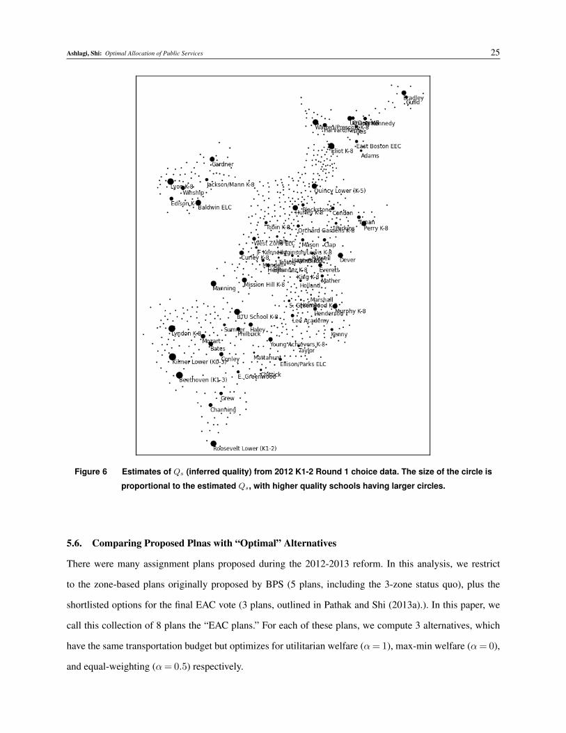
displayed in Figure 6.
5.5. Defining the Objective and Constraints
For the purpose of this empirical exercise, we assume that the objective of the assignment plan is of the
form in Section 4, which is to maximize a linear combination of the average expected utility of students and
the minimum expected utility for a type W (x) = α∑
twtvt + (1−α)mint vt, where wt is proportional to
the number of students of that type, with∑
twt = 1, vt =Eu∝Ft [u ·xt] is the expected utility of a student of
type t, and α is a parameter specifying the desired trade-off between efficiency and equity. α= 1 represents
utilitarian welfare; α= 0 represents max-min welfare; α= 0.5 represents an equal weighting of the two.
To account for transportation costs, we require that an assignment plan stays within a budget of a certain
number of miles of busing per student27:∑
twtDtsE[xts] ≤ B. Note that in reality, busing cost is much
more complicated, having to do with the routing, the types and number of buses used, the presence of
Special Education programs which require the more expensive door-to-door busing, etc. We leave finer
modeling of transportation costs to future work.
25 This is estimated using Google Maps walk distance from the centroid of the student’s geocode to the centroid of the school’sgeocode.26 We adopt the specification called “Simple” in Pathak and Shi (2013b), estimated using 2012 Round 1 choice data, aggregatinggrades K1 and K2. We assume that all programs are Regular Education.27 The denominator includes all students, not only those who are bused positive amounts.
Ashlagi, Shi: Optimal Allocation of Public Services 25
Figure 6 Estimates of Qs (inferred quality) from 2012 K1-2 Round 1 choice data. The size of the circle is
proportional to the estimated Qs, with higher quality schools having larger circles.
5.6. Comparing Proposed Plnas with “Optimal” Alternatives
There were many assignment plans proposed during the 2012-2013 reform. In this analysis, we restrict
to the zone-based plans originally proposed by BPS (5 plans, including the 3-zone status quo), plus the
shortlisted options for the final EAC vote (3 plans, outlined in Pathak and Shi (2013a).). In this paper, we
call this collection of 8 plans the “EAC plans.” For each of these plans, we compute 3 alternatives, which
have the same transportation budget but optimizes for utilitarian welfare (α= 1), max-min welfare (α= 0),
and equal-weighting (α= 0.5) respectively.

26 Ashlagi, Shi: Optimal Allocation of Public Services
The EAC plans are as follows.28 There are 6 zone-based plans: 3-zone (status quo), 6-zone, 9-zone, 10-
zone, 11-zone, and 23-zone respectively. There are two non-zone-based plans. In the first, called “Home
Based A” by BPS, families can choose the union of the schools within their walk-zone, the 2 closest Tier
1 schools, the 4 closest Tier 1 or 2 schools, the 6 closest Tier 1, 2 or 3 schools, as well as the 3 closest
“capacity schools” (schools projected to be the least over-demanded relative to their capacity). The second
plan, Home Based B, is similar except the counts 2, 4, 6, 3 are replaced by 3, 6, 9, 3 respectively. For these
plans, the EAC chose to remove the walk-zone priority. In this analysis, we assume that each zoned plan
has walk-zone priority and that each Home Based plan does not.
To quantify the performance of these plans under our soft capacity limit setting, we utilize the fact,
shown in Appendix A, that in the large market whether the capacity limit is hard or soft matters little in a
proportional sense. Hence, we simply take all of current BPS students in K2-5 (24759 students), simulate
their choices to the 75 available schools (26448 K2-5 seats) using the random utility model in Section 5.4,
and simulate the Deferred Acceptance algorithm outlined in Section 5.1. This yields an assignment. For
each students type and each school, we compute the worst lottery number needed for an additional student
of this type to get into this school, and set this as the lottery cutoff to this school for this type. This works
because one can reproduce the original assignment using these lottery cutoffs and the realized choices.29
This allows us to represent all of the EAC plans as lottery-plus-cutoffs plans.
Given a lottery-plus-cutoffs plan, the proof of Proposition 1 shows how to represent it as randomized
menus, and the formula in Section 4 for vt(M) and pt(s,M) can be used to compute the utilitarian wel-
fare, the max-min welfare, and the average distance bused. Setting the averaged distance bused to be the
transportation budget, and letting α to be 1 or 0, we can compute the optimal utilitarian welfare or max-min
welfare using the same (or less) amount of transportation. The computation was done up to a 1% optimality
gap. This traces out the “Pareto frontiers” trading off a measure of cost with a measure of welfare. Figure 7
show these Pareto frontiers as well as the performance of the other plans. For utilitarian welfare (Figure 7a),
α= 1 represents the Pareto frontier; for max-min welfare (Figure 7b, α= 0 is the Pareto frontier. As seen in
the figures, while optimizing purely for utilitarian welfare (α= 1) or for max-min welfare (α= 0) may sac-
rifice the other measure, the equal-weighting (α= 0.5) achieves near-optimal performance with respect to
both, dominating the original EAC plans in both measures. This suggests that setting α= 0.5 is an effective
way to optimize efficiency in an equitable way.
We also compare the plans in terms of predictability. One measure of predictability is the probability
of getting one’s first choice. In Figure 8, we compare the EAC plans with the optimized plans with α ∈
{0,0.5,1}. As seen, all of the optimized plans improve over the EAC plans in this measure of predictability,
28 For details, see BPS (2013a) and Pathak and Shi (2013a).29 The correspondence between a stable matching, which is the output from any Deferred Acceptance procedure, and a set of cutoffs,is shown in Azevedo and Leshno (2012).

Ashlagi, Shi: Optimal Allocation of Public Services 27
(a) Utilitarian Welfare (b) Max-min WelfareFigure 7 Comparing the EAC plans with optimized plans (α∈ {0,0.5,1}) in terms of utilitarian and max-min
welfare. The α= 0.5 line is often indistinguishable from the Pareto frontiers (α= 1 in the left and α= 0 in the
right).
although predictability is not explicitly optimized in the computation. The utilitarian plans (α= 1) achieve
almost 100% probability of getting into first choice school, because since our utility model is roughly quality
minus distance, to maximize sum of expected utilities the plan limits schools to the closest students in such
a way that “just enough” students are included. The α = 0.5 of α = 0 plans may use lottery to improve
equity (max-min welfare) but are still more predictable than the EAC plans in terms of getting first choice.
Figure 8 Comparing the EAC plans with the optimized plans (α∈ {0,0.5,1}) in terms of average probability
of getting into first choice.
5.7. In-Depth Comparison of the Chosen EAC Plan with a Corresponding “Optimal” Alternative
In this section, we compare in detail the plan adopted by the EAC, Home Based A, with the “optimal”
alternative with the same transportation budget but optimizing the equal-weighting objective (α= 0.5). For

28 Ashlagi, Shi: Optimal Allocation of Public Services
Home Based A Opt AUtilitarian Welfare 10.9 11.4Max-min Welfare 7.7 11.1Prob. Getting First Choice 65% 85%Av. Miles Bused 0.37 0.37
Table 2 Side by side comparison of the plan chosen by the EAC (Home Based A) with an optimized
alternative (Opt A), which uses the same transportation budget and equal-weighting objective (α= 0.5). As
seen, the optimized plan improves in all aspects of utilitarian welfare (“efficiency”), max-min welfare
(“equity”) and probability of getting first choice (“predictability”). The units of welfare is in miles, since
distance has coefficient 1 in the utility model.
simplicity, we call this plan “Opt A.” Table 2 shows the summary of these two plans with respect to a variety
of metrics.
For any plan, define the catchment region of a school as the geocodes from which students have positive
probability of getting in the school. It is instructive to visually inspect the catchment regions and cutoffs
in the two assignment plans. Figure 9 examines a school considered to be of higher quality and in a richer
neighborhood of Boston. It illustrates the idea that for a higher quality school, Opt A offers it to students
who live closer and with higher probability (increasing efficiency as utility is discounted by distance), while
possibly also offering it to “problem areas” that otherwise have low expected utility (increasing equity).
Figure 10 examines a school considered to be of lower quality and in a poorer neighborhood of Boston. It
illustrate the idea that for a lower quality school, Opt A offers it to a larger region. This makes sense in our
model because since we assume that students are choosing according to our utility model, they would only
choose far away lower quality schools if they have large idiosyncratic preference for them, and so it is in
the city’s best interest to provide transportation in this case since it both satisfies these students and opens
up space to the better quality schools in these students’ home neighborhoods.
We validate the above insights systematically in Figure 11. The figure compares the catchment area (size
of the catchment region) in these two plans for schools of various inferred quality, aggregating by quartile
of quality Qs. As shown, Opt A exhibits smaller access regions for the top 2 quartiles, while offering the
lowest quality schools to much larger areas.
We now compare the choice menus in these two plans (for each geocode, what are the schools that
students at the geocode can access with positive probability). We first show some examples. Figure 12a
shows the choice menu in both Home Based A and Opt A for a student living on the suburban boundary
of the richer West Roxbury section of the city, which according to Figure 6 has a few good quality schools
in the neighborhood. Figure 12b shows the menus for a student living in the poorer Mattapan area of the
city. This is one of the “problem areas” identified by BPS, as confirmed by Figure 6, which shows that the
schools in this neighborhood are mostly of lower inferred quality.
In both plans, students living near bad schools are given more choices, but Opt A does this much more
aggressively than Home Based A. Figure 12 compares the choice menu of two students: the first lives near

Ashlagi, Shi: Optimal Allocation of Public Services 29
Figure 9 The cutoffs in Home Based A (left) and Opt A (right) to Lyndon (one of the higher quality schools
in the richer West Roxbury neighborhood of Boston). The circles represent the catchment region. The color of
each circle represents the cutoff, and the histogram on the right shows the distribution of cutoffs. In Home
Based A (left), all the geocodes in the catchment region have about 90% probability of getting into this school
if they choose it first. In Opt A (right), while the region closest to Lyndon has 100% chance of getting into
Lyndon if they choose it first, there is a further away yellow region from which students can get into Lyndon
with a good lottery number.
mostly higher quality schools and the second lives near mostly lower quality schools. Home Based A gives
the first student 8 choices and the second student 11, while Opt A gives the first student 3 and the second
student 55. Examining the inferred school qualities in Figure 6 shows that under Opt A, the second student
essentially gets every lower quality school in the city. This is a very dramatic move to compensate her for
living near lower quality schools.
Figure 13 illustrates this “quantity-quality-trade-off” systematically. It plots for each geocode the number
of choice options students living there are offered versus the average qualityQs of these schools. As shown,
while the best-fit line for Home Based A shows a negative slope of −3.46, the trade-off for Opt A is much
steeper, with slope −10.78. This means that if the average quality decreases by 1 unit (measured in miles),
the student is on average given 3.46 more options in Home Based A and 10.78 more options in Opt A.
6. DiscussionIn this paper, we build a tractable and empirically relevant framework for a social planner to design the
optimal mechanism to allocate public services, without requiring either monetary transfers or costly sig-
nals. The analysis relies assumptions of soft capacity limits and Pareto-optimality (within types) of interim
allocation rules, so our results are most applicable in cases when these are reasonable. One such case is

30 Ashlagi, Shi: Optimal Allocation of Public Services
Figure 10 The cutoffs in Home Based A (left) and Opt A (right) to Taylor (one of the lower quality schools in
the poorer Mattapan neighborhood of Boston). The circles represent the catchment region. The color of each
circle represents the cutoff, and the histogram on the right shows the distribution of cutoffs. In Home Based A
(left), all the geocodes in the catchment region have about 85% probability of getting into this school if they
choose it first. In Opt A (right), the catchment region is larger and the cutoffs are also higher. (This is possible
with the same capacity limits because the catchment region in Opt A for Taylor has better alternatives so
fewer students are expected to choose Taylor.)
Figure 11 Comparison of catchment area in Home Based A versus Opt A for schools of various inferred
quality (Qs from the utility model). The averages for each quartile of quality is shown, with Q1 being the
schools with top 25% quality, Q2 being the next 25%, and so on. As can be seen, while the catchment areas in
Home Based A exhibit no clear trend as quality decreases, the catchment area for Opt A increases with
decreasing quality, with the lowest quality schools having very large catchment area (over 22 square miles on
average).

Ashlagi, Shi: Optimal Allocation of Public Services 31
(a) A student living near higher quality schools (b) A student living near lower quality schoolsFigure 12 Comparing choice menus in Home Based A (blue squares) and Opt A (red pluses). The location
of the student is the green circle. Left shows a student living in the suburban boundary of the richer West
Roxbury section of the city, where schools in the neighborhood are of higher quality (See Figure 6). Since, the
3 closest schools, Kilmer, Beethoven, and Lyndon are all of relatively high quality, Opt A finds it sufficient to
only give her these schools. Right shows a student living in the poorer Mattapan section of the city, where
schools in the neighborhood are of lower quality. In trying to compensate the student, Opt A gives her many
more choices.
the “large market” scenario, in which there are many agents per type and many slots per service. In this
setting, soft capacity limits mimic hard capacity limits. Moreover, Pareto-optimality of interim allocation
rules becomes equivalent to requiring that agents do not have incentives to trade within types ex-post, which
is because if there are positive gains to be realized from trading and there are many agents, one may expect
trading to occur and it may be difficult to prevent it by enforcement. So a social planner should take this
into account in designing the mechanism.
A problem for future work is the efficient computation of the optimal cardinal mechanism. After discretiz-
ing the prices, our current techniques can reduce this to an exponential sized linear program, but we have
not found any interesting distributions for which we can efficiently solve the optimal-menu subproblem.
In applying our techniques for computing the optimal ordinal mechanism in practice, it is important
to check whether the modeling assumptions correspond to reality. For example, if one were to apply our
techniques to make real policy recommendations for Boston, one would have to more carefully model the

32 Ashlagi, Shi: Optimal Allocation of Public Services
Figure 13 The quantity-quality tradeoff in Home Based A and Opt A. Home Based A is in blue squares and
Opt A is in red plus. Each point represents a geocode (type), with the size of the point representing the
number of students residing at that geocode (weight of the type). The x axis is average quality Qs of schools
in the menu of that geocode, and the y axis is the size of the menu. As seen, Opt A compensates for quality by
increasing quantity much more aggressively than Home Based A, in hope that the idiosyncratic taste
component to one of these additional schools is high.
objective and constraints and confer with policy makers and key stakeholders. Furthermore, whether our
computed “optimal” mechanism is reasonable depends crucially on the validity of the utility model. For
example, if it turns out that the idiosyncratic taste shocks of individuals are very correlated (instead of being
independent as we assumed) or exhibit thinner tails than the Gumbel distribution, then our “optimal” plan
would not be able to sufficiently compensate those who live near lower quality schools by offering a huge
variety of low quality options. (Under the assumptions in this paper, this does give sufficient compensation
because if idiosyncratic taste shocks are independent and have thick tails, then given a large enough menu, a
family is bound to have high taste shock to some school.) Such a plan would also be undesirable if families
have significant “search costs” in processing large menus or perceive “fairness” in a different way, such
as in terms of access to particular schools instead of in terms of utilities. Accounting for these requires
studying the “behavioral” aspects of school choice. Finding a more realistic utility model for school choice
is a subject for future work.
Ashlagi, Shi: Optimal Allocation of Public Services 33
ReferencesAbdulkadiroglu, Atila, Y.K. Che, Y. Yasuda. 2008. Expanding “choice” in school choice. Available at http://
papers.ssrn.com/sol3/papers.cfm?abstract_id=1308730.
Abdulkadiroglu, Atila, Parag A. Pathak, Alvin E. Roth. 2009. Strategy-proofness versus efficiency in matching with
indifferences: Redesigning the nyc high school match. American Economic Review 99(5) 1954–1978.
Abdulkadiroglu, Atila, Parag A. Pathak, Alvin E. Roth, Tayfun Sonmez. 2005. The boston public school match.
American Economic Review, Papers and Proceedings 95 368–371.
Abdulkadiroglu, Atila, Parag A. Pathak, Alvin E. Roth, Tayfun Sonmez. 2006. Changing the boston school choice
mechanism. Boston College Working Papers in Economics 639, Boston College Department of Economics.
Abdulkadiroglu, Atila, Tayfun Sonmez. 2003. School choice: A mechanism design approach. American Economic
Review 93 729–747.
Ashlagi, Itai, Peng Shi. 2013. Improving community cohesion in school choice via correlated-lottery implementation.
Available at http://www.mit.edu/˜pengshi/papers/community-cohesion.pdf.
Azevedo, Eduardo M., Jacob D. Leshno. 2012. A supply and demand framework for two-sided matching markets.
Available at http://www.people.fas.harvard.edu/˜azevedo/papers/azevedo_jmp.pdf.
Bogomolnaia, Anna, Herve Moulin. 2001. A new solution to the random assignment problem. Journal of Economic
Theory 100(2) 295–328.
BPS. 2012a. Boston public schools: Improving school choice. http://bostonschoolchoice.wordpress.
com/.
BPS. 2012b. Fiscal year 2013 preliminary budget cover memo. Available at http://www.
bostonpublicschools.org/files/2012-2-1_fy13_preliminary_budget_cover_memo.
pdf.
BPS. 2012c. How does the bps school choice process work? Available at www.bostonpublicschools.org/
files/studentassign2pagefinal.pdf.
BPS. 2013a. Improving school choice. http://bostonschoolchoice.org/.
BPS. 2013b. Preliminary transportation analysis. Available at http://bostonschoolchoice.files.
wordpress.com/2013/02/2013-02-20-transportation-cost-analysis-final.pdf.
Braverman, Mark, Jing Chen, Sampath Kannan. 2013. Optimal provision-after-wait in healthcare. Available at http:
//www.cs.princeton.edu/˜mbraverm/pmwiki/index.php?n=Research.AllPapers.
Budish, Eric. 2011. The combinatorial assignment problem: Approximate competitive equilibrium from equal
incomes. Journal of Political Economy 119(6) 1061–1103.
Budish, Eric, Estelle Cantillon. 2012. The multi-unit assignment problem: Theory and evidence from course allocation
at harvard. American Economic Review 102(5) 2237–71.

34 Ashlagi, Shi: Optimal Allocation of Public Services
Chakravarty, Surajeet, Todd R. Kaplan. 2013. Optimal allocation without transfer payments. Games and Economic
Behavior 77 1–20.
Che, Yeon-Koo, F. Kojima. 2011. Asymptotic equivalance of probabilistic serial and random priority mechanisms.
Econometrica 78(5) 1625–1672.
Cole, Richard, Vasilis Gkatzelis, Gagan Goel. 2013. Positive results for mechanism design without money. Pro-
ceedings of the 2013 international conference on Autonomous agents and multi-agent systems. AAMAS ’13,
International Foundation for Autonomous Agents and Multiagent Systems, Richland, SC, 1165–1166.
Condorelli, Daniele. 2012. What money cant buy: Efficient mechanism design with costly signals. Games and
Economic Behavior 75(2) 613–624.
EAC. 2013. Recommendations by the external advisory committee (eac) on school choice.
Available at http://bostonschoolchoice.files.wordpress.com/2013/03/
5-eac-recommendations-draft-feb-25-revised.docx.
Ebbert, Stephanie, Jenna Russell. 2011. A daily diaspora, a scattered street. The Boston Globe (12 Jun. 2011).
Ehlers, Lars, Isa Hafalir, Bumin Yenmez, Muhammed Yildirim. 2011. School choice with controlled choice con-
straints: Hard bounds versus soft bounds. GSIA Working Papers 2012-E20, Carnegie Mellon University, Tepper
School of Business.
Erdil, A, H. Ergin. 2008. What’s the matter with tie-breaking? improving efficiency in school choice. American
Economic Review 95.
Guo, Mingyu, Vincent Conitzer. 2010. Strategy-proof allocation of multiple items between two agents without pay-
ments or priors. Proceedings of the 9th International Conference on Autonomous Agents and Multiagent Sys-
tems: volume 1 - Volume 1. AAMAS ’10, International Foundation for Autonomous Agents and Multiagent
Systems, Richland, SC, 881–888.
Hartline, Jason D., Tim Roughgarden. 2008. Optimal mechanism design and money burning. Proceedings of the 40th
annual ACM symposium on Theory of computing. STOC ’08, ACM, New York, NY, USA, 75–84.
He, Yinghua, Antonio Miralles, Jianye Yan. 2012. Competitive equilibrium from equal incomes for two-sided match-
ing. Working Papers 692, Barcelona Graduate School of Economics.
Hylland, Aanund, Richard Zeckhauser. 1979. The efficient allocation of individuals to positions. Journal of Political
Economy 87(2) 293–314.
Krishna, Aradhna, M. Utku Unver. 2006. Improving the efficiency of course bidding at business schools: Field and
laboratory studies. Marketing Science 27(2) 262–282.
Krishna, Vijay. 2002. Auction Theory. Academic Press.
Lilly, Dick. 2009. It’s back to neighborhood schools for seattle. Crosscut (7 Oct. 2009).
Liu, Qingming, Marek Pycia. 2012. Ordinal efficiency, fairness, and incentives in large markets. Avalable at http:
//pycia.bol.ucla.edu/liu-pycia-large.pdf.

Ashlagi, Shi: Optimal Allocation of Public Services 35
Menino, Thomas. 2012. The honorable mayor thomas m. menino state of the city address. Available at http:
//www.cityofboston.gov/mayor/speech.asp.
Milgrom, P.R. 2004. Putting Auction Theory to Work. Churchill Lectures in Economics, Cambridge University Press.
Miralles, Antonio. 2012. Cardinal bayesian allocation mechanisms without transfers. Journal of Economic Theory
147 179–206.
Myerson, Roger B. 1981. Optimal auction design. Mathematics of operations research 6(1) 58–73.
Pathak, Parag A. 2011. The mechanism design approach to student assignment. Annual Review of Economics 3.
Pathak, Parag A., Peng Shi. 2013a. Simulating alternative school choice options in boston. Tech. rep., MIT School
Effectiveness and Inequality Initiative.
Pathak, Parag A., Peng Shi. 2013b. Simulating alternative school choice options in boston - technical appendix. Tech.
rep., MIT School Effectiveness and Inequality Initiative.
Roth, A. E., A. Postlewaite. 1977. Weak versus strong domination in a market with indivisible goods. Journal of
Mathemnatical Economics 4 131–137.
Russell, Jenna, Stephanie Ebbert. 2011. The high price of school assignment. The Boston Globe (12 Jun. 2011).
Russell, Jenna, Stephanie Ebbert, James Vaznis. 2011. Getting in: Inside boston’s school assignment maze. Available
at http://www.boston.com/news/education/specials/school_chance/articles/.
Ryan, Andrew, James Vaznis. 2012. Menino vows change in school assignment system. Boston Globe (18 Jan. 2012).
Schummer, James, Rakesh Vohra. 2007. Mechanism design without money. Noam Nisan, Tim Roughgarden, Eva
Tardos, Vijay V. Vazirani, eds., Algorithmic Game Theory. Cambridge University Press, Cambridge, UK, 243–
266.
Seelye, Katharine Q. 2013a. Boston schools drop last remnant of forced busing. New York Times (14 Mar. 2013).
Seelye, Katharine Q. 2013b. No division required in this school problem. New York Times (12 Mar. 2013).
Shapley, L., H. Scarf. 1974. On cores and indivisibility. Journal of Mathemnatical Economics 1 23–28.
Sonmez, Tayfun, M. Utku Unver. 2010. Course bidding at business schools. International Economic Review 51(1)
99–123.
Sutherland, Amy. 2012. To bus or not: Bostons school-choice program. BU Today (2012).
Thomson, W., L. Zhou. 1993. Consistent allocation rules in atomless economies. Econometrica 61(3) 575–587.
Varian, Hal R. 1974. Equity, envy, and efficiency. Journal of Economic Theory 9 63–91.
Woodward, Mikala. 2011. Southeast seattle schools: World war ii to present. Available at www.seattle.gov/
neighborhoods/preservation/southeastseattle.
Zhou, Lin. 1992. Strictly fair allocations in large exchange economies. Journal of Economic Theory 57(1).

36 Ashlagi, Shi: Optimal Allocation of Public Services
Appendix A: Another View of Soft Capacity Limits: Large Market
In our formulation, we used soft capacity-limits to justify considering only interim allocation rules, which greatly
simplifies analysis. One intuition is that in a large market, because the Law of Large Numbers average away stochas-
tic variations, there is not much difference between soft and hard capacity-limits. So even if one does not find soft
capacity-limit to be reasonable, one can justify our analysis as a reasonable approximation of the hard capacity-limits
case when the market is large. The following results make precise this intuition.
DEFINITION 6. For type t, given a cardinal or ordinal interim allocation rule xt, its independent implementation is
to assign each agent service s according to probability xts independently for all agents of that type. (xts depends on
the agent’s preference report.)
The following proposition shows that when the market is large, for an independent implementation of an interim
allocation rule allocates, the probability, that the number of slots allocated for service s exceeds (1 + ε) times the
expected number, decays exponentially with the size of the market. This implies that the independent implementation
of a mechanism that satisfies soft-capacity constraints would approximately satisfy hard capacity-constraints with high
probability in the large market. This result follows immediately from multiplicative Chernoff bounds.
PROPOSITION 3. For type t, given cardinal interim allocation rule xt, the ex-ante expected number of slots of
service s allocated to this type is ms = |It|xts(U). For any ε > 0, its independent implementation assigns more than
(1 + ε)ms slots of service s with probability at most exp(−δ(ε)ms), where δ(ε) = (1 + ε)log(1 + ε)− ε > 0. The same
is true for ordinal interim allocation rule if we replace U with Π.
Appendix B: Omitted Proofs
LEMMA 1. An interim cardinal allocation rule is incentive compatible if and only if there exists closed convex set
X ⊆∆ such that x(u)∈ arg maxy∈X{u ·y}, ∀u∈U .
Proof of Lemma 1 Suppose cardinal interim allocation rule x(u) is incentive compatible. Let X be the convex
closure of its range. Then since u · x(u) ≥ u · x(u′)∀u′ ∈ U , we have u · x(u) ≥ u · y ∀y ∈ X . So x(u) ∈arg maxy∈X{u ·y}.
Conversely, if for some closed convex set X , for any u∈U , x(u)∈ arg maxy∈X{u ·y}, then ∀u′ ∈U , x(u′)∈X ,
so u ·x(u)≥ u ·x(u′). So x is incentive compatible. �
LEMMA 2 Any tangent hyperplane of X in lin(∆) can be written as H(a,1) ∩ lin(∆), for some a ∈ (0,∞)|S|,
with a pointing outward from X and not co-linear with 1. (a ·y≤ 1, ∀y ∈X , and a 6= λ1 for any λ∈R.)
Proof of Lemma 2 Any tangent hyperplane Y of X in lin(∆) is a |S| − 2 dimensional subspace of the |S| − 1
dimensional linear space lin(∆). Take an arbitrary point z ∈∆ on the same side of Y as X . Consider the |S| − 1
dimensional hyperplane H passing through Y and (1 + ε)z. For some sufficiently small ε > 0, by continuity, H has
all positive intercepts, so H = {y : a · y ≤ 1} for some a > 0, and by construction, a is not co-linear with 1. Now,
a · z= 11+ε
< 1, so a points outward from X . �
LEMMA 3 If X is a closed convex set that corresponds to incentive compatible interim cardinal allocation rule x.
Suppose that H(a,1) is an outward pointing supporting hyperplane of X that intersects X in the relative interior of
the feasibility simplex, int(∆). Then for any unit vector d∈U such that d ·a> 0, there exists δ0 > 0 such that for all
δ ∈ (0, δ0), there exists interim allocation rule x′ that strictly dominates x, with x′(U) = x(U) + δd.
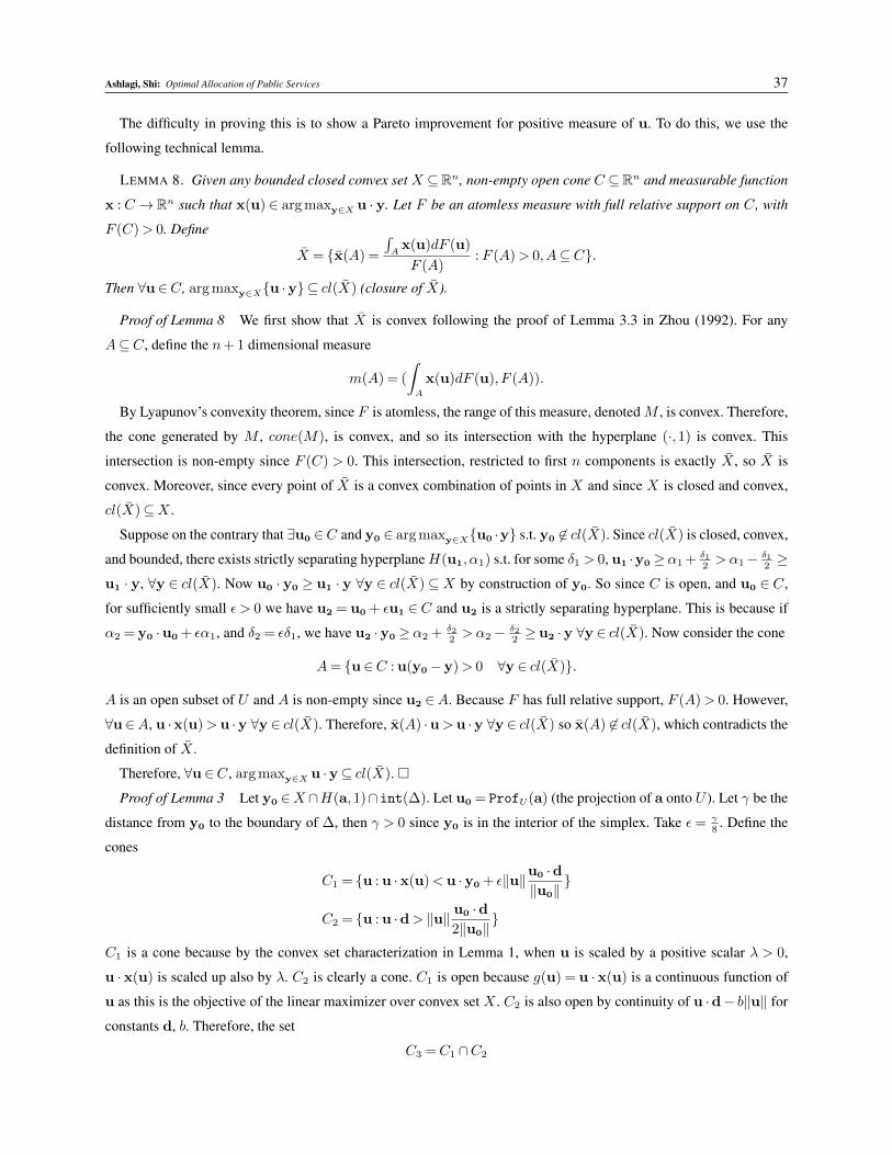
Ashlagi, Shi: Optimal Allocation of Public Services 37
The difficulty in proving this is to show a Pareto improvement for positive measure of u. To do this, we use the
following technical lemma.
LEMMA 8. Given any bounded closed convex set X ⊆Rn, non-empty open cone C ⊆Rn and measurable function
x : C→ Rn such that x(u) ∈ arg maxy∈X u · y. Let F be an atomless measure with full relative support on C, with
F (C)> 0. Define
X = {x(A) =
∫Ax(u)dF (u)
F (A): F (A)> 0,A⊆C}.
Then ∀u∈C, arg maxy∈X{u ·y} ⊆ cl(X) (closure of X).
Proof of Lemma 8 We first show that X is convex following the proof of Lemma 3.3 in Zhou (1992). For any
A⊆C, define the n+ 1 dimensional measure
m(A) = (
∫A
x(u)dF (u), F (A)).
By Lyapunov’s convexity theorem, since F is atomless, the range of this measure, denotedM , is convex. Therefore,
the cone generated by M , cone(M), is convex, and so its intersection with the hyperplane (·,1) is convex. This
intersection is non-empty since F (C) > 0. This intersection, restricted to first n components is exactly X , so X is
convex. Moreover, since every point of X is a convex combination of points in X and since X is closed and convex,
cl(X)⊆X .
Suppose on the contrary that ∃u0 ∈C and y0 ∈ arg maxy∈X{u0 ·y} s.t. y0 6∈ cl(X). Since cl(X) is closed, convex,
and bounded, there exists strictly separating hyperplaneH(u1, α1) s.t. for some δ1 > 0, u1 ·y0 ≥ α1 + δ12>α1− δ1
2≥
u1 · y, ∀y ∈ cl(X). Now u0 · y0 ≥ u1 · y ∀y ∈ cl(X)⊆X by construction of y0. So since C is open, and u0 ∈ C,
for sufficiently small ε > 0 we have u2 = u0 + εu1 ∈C and u2 is a strictly separating hyperplane. This is because if
α2 = y0 ·u0 + εα1, and δ2 = εδ1, we have u2 ·y0 ≥ α2 + δ22>α2− δ2
2≥ u2 ·y ∀y ∈ cl(X). Now consider the cone
A= {u∈C : u(y0−y)> 0 ∀y ∈ cl(X)}.
A is an open subset of U and A is non-empty since u2 ∈A. Because F has full relative support, F (A)> 0. However,
∀u∈A, u ·x(u)> u ·y ∀y ∈ cl(X). Therefore, x(A) ·u> u ·y ∀y ∈ cl(X) so x(A) 6∈ cl(X), which contradicts the
definition of X .
Therefore, ∀u∈C, arg maxy∈X u ·y⊆ cl(X). �
Proof of Lemma 3 Let y0 ∈X ∩H(a,1)∩int(∆). Let u0 = ProfU(a) (the projection of a onto U ). Let γ be the
distance from y0 to the boundary of ∆, then γ > 0 since y0 is in the interior of the simplex. Take ε= γ
8. Define the
cones
C1 = {u : u ·x(u)< u ·y0 + ε‖u‖u0 ·d‖u0‖
}
C2 = {u : u ·d> ‖u‖ u0 ·d2‖u0‖
}
C1 is a cone because by the convex set characterization in Lemma 1, when u is scaled by a positive scalar λ > 0,
u · x(u) is scaled up also by λ. C2 is clearly a cone. C1 is open because g(u) = u · x(u) is a continuous function of
u as this is the objective of the linear maximizer over convex set X . C2 is also open by continuity of u ·d− b‖u‖ for
constants d, b. Therefore, the set
C3 =C1 ∩C2

38 Ashlagi, Shi: Optimal Allocation of Public Services
is an open cone. Moreover, it is non-empty since u0 ∈C3.
Now, X is bounded, closed and convex. C3 is a non-empty open cone. Therefore by Lemma 8, y0 ∈
arg maxy∈X{u0 · y} ⊆ cl(X), so there exists A ⊆ C3, F (A) > 0, s.t. ‖x(A) − y0‖ ≤ ε u0·d‖u0‖
. Now, consider the
alternative interim allocation rule
y(u) =
{x(A) + 6εd if u∈Ax(u) otherwise.
y(u)∈∆ ∀u∈U since 7ε < γ.
By construction, y(U) = x(U) + 6εF (A)d. Moreover, y strictly Pareto improves x because ∀u∈A,
u · x(A) + 6εu ·d−u ·x(u)
>u ·y0− εu0 ·d‖u0‖
‖u‖+ 3ε‖u‖u0 ·d‖u0‖
−u ·x(u)
>ε‖u‖u0 ·d‖u0‖
>0
Now, let δ0 = 6εF (A), for any δ ∈ (0, δ0), if we set
x′(u) =δ
δ0y(u) + (1− δ
δ0)x(u).
Then x′ still strictly Pareto improves x since objectives are linear, but x′(U) = x(U) + δd, which is what we needed.
�
LEMMA 4 An interim ordinal allocation rule x(π) is incentive compatible if and only if there exists monotone
submodular set function f : 2|S|→ [0,1] s.t. ∀1≤ k≤ |S|,
xπ(k)(π) = f({π(1), · · · , π(k)})− f({π(1), · · · , π(k− 1)}).
Proof of Lemma 4. If x(π) is an incentive compatible interim ordinal allocation rule, then for any M ⊆ S, define
f(M) =
|M|∑j=1
xπ(j)(π), where{π(1), π(2), · · · , π(|M |)}=M.
This is well-defined because incentive compatibility requires each agent’s chances of getting a service in M , condi-
tional on ranking these first in some order (ranking all of M before all of S\M ), to be fixed, regardless of the relative
rank between services in M and services in S\M . If this were not the case, then for some large b > 0 and small ε≥ 0,
consider an agent with utilities us = b+ εs for s∈M and us =−c+ εs, where {εs < ε} are small distinct numbers that
sum to zero, and c = b|M |/(|S| − |M |) is set to preserve normalization∑
sus = 0. If the agent’s chance of getting
a service in M can be altered by changing relative order in M and relative order in S\M , while she ranks M before
S\M , then the agent would for some {εs}’s gain b times a positive number and lose at most |S|ε, so for sufficiently
large bε
she has incentive to mis-report.
We now show that f is submodular. Suppose on the contrary that f is not submodular, then there exists M1 ⊆M2,
and s 6∈M2, such that
f(M1 ∪{s})− f(M1)< f(M2 ∪{s})− f(M2).

Ashlagi, Shi: Optimal Allocation of Public Services 39
However, for sufficiently large b, let us = b for s ∈M1 ∪ {s}, and us = −c for s ∈M2\M1, where c = b(|M1|+1)/(|M2|) is set to preserve the normalization
∑sus = 0. She would have incentive to rank elements of M2\M1
before s and improve expected utility. This contradicts incentive compatibility.
Now, the construction of f implies f is monotone, and that ∀π ∈ Π and 1 ≤ k ≤ |S|, xπ(k)(π) =
f({π(1), · · · , π(k)})− f({π(1), · · · , π(k− 1)}).
Conversely, if f is a monotone submodular set function. We show that if we define x so that xπ(k)(π) =
f({π(1), · · · , π(k)})− f({π(1), · · · , π(k− 1)}), then x is incentive compatible. Note that the range of x defined this
way is simply the vertex set of the base polytope of the polymatroid defined by f :∑s∈M
xs ≤ f(M) ∀M ⊆ S∑s∈S
xs = 1
xs ≥ 0 ∀s∈ S.
Now, the agent’s utility u · x is linear in x, so using the fact that the greedy algorithm optimizes a linear objective
over a polymatroid (and also the base polytope), we get that for any u, if we re-label S so that
u1 ≥ u2 ≥ · · · ≥ u|S|.
Then an optimal point of the base polytope simply sets x1 to f({1}), and x2 to f({1,2})− f({1}) and so on, which
is exactly how we defined x. Thus, x(π)∈ arg maxπ′∈Π u ·x(π′), and x is incentive compatible. �
LEMMA 5 Let f be the monotone submodular set function that corresponds to incentive compatible interim allo-
cation rule x. If x is ordinal efficient, then for any M1,M2 ⊆ S,
f(M1 ∪M2) = max{f(M1), f(M2)}.
Proof of Lemma 5. By monotonicity of f , f(M1 ∪M2) ≥max{f(M1), f(M2)}. What we need to show is that
f(M1 ∪M2)≤max{f(M1), f(M2)}. By monotonicity, it suffices to show this for the case in which M1 ∩M2 = ∅.Suppose that on the contrary that f(M1 ∪M2) > max{f(M1), f(M2)}, M1 ∩M2 = ∅. Consider two preference
rankings, π1 and π2: π1 ranks services in M1 first, followed by M2, followed by other services in arbitrary order;
π2 ranks services in M2 first, followed by M1, followed by others. By Lemma 4, since x is incentive compatible,∑s∈M2
x(π1) = f(M1 ∪M2) − f(M1) > 0, and∑
s∈M1x(π2) = f(M1 ∪M2) − f(M2) > 0. Thus, agents with
preference ranking π1 can trade probabilities with agents with preference ranking π2 and mutually improve in the
first-order stochastic dominance sense. (Agents preferring M1 get additional probabilities for services in M1 in place
of equal probabilities for M2, while agents preferring M2 get additional probabilities for M2 in place of M1.) By full
relative support, there exist positive measures of both kinds of agents, so x is not ordinal efficient, contradiction. �
LEMMA 6 µt(γ,λ,ν) is convex.
Proof of Lemma 6. Given γ′, λ′, ν′ and γ′′,λ′′, ν′′. If (γ,λ,ν) = y(γ′,λ′,ν′) + (1− y)(γ′′,λ′′,ν′′) for y ∈[0,1], then if M∗ ∈ arg maxM⊆S ft(γ,λ,ν,M), then
µt(γ,λ,ν) = ft(γ,λ,ν,M∗)
= yft(γ′,λ′,ν′,M∗) + (1− y)ft(γ
′′,λ′′,ν′′,M∗)
≤ yµt(γ′,λ′,ν′) + (1− y)µt(γ′′,λ′′,ν′′)
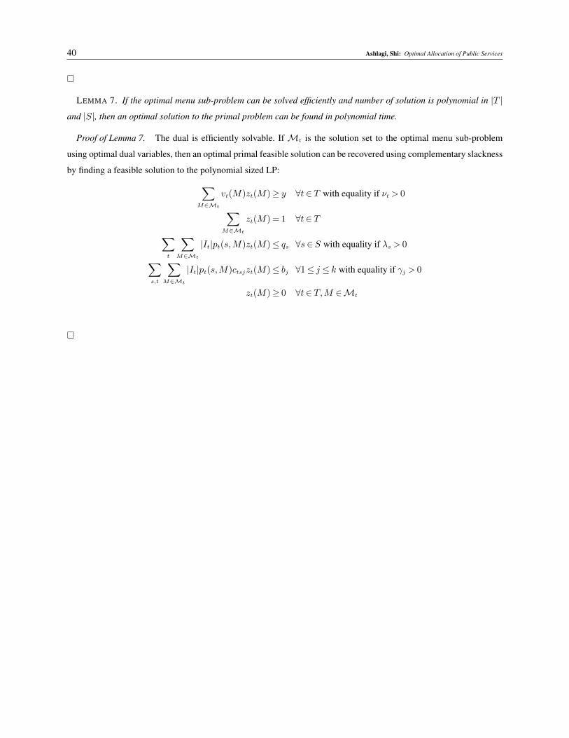
40 Ashlagi, Shi: Optimal Allocation of Public Services
�
LEMMA 7. If the optimal menu sub-problem can be solved efficiently and number of solution is polynomial in |T |
and |S|, then an optimal solution to the primal problem can be found in polynomial time.
Proof of Lemma 7. The dual is efficiently solvable. If Mt is the solution set to the optimal menu sub-problem
using optimal dual variables, then an optimal primal feasible solution can be recovered using complementary slackness
by finding a feasible solution to the polynomial sized LP:∑M∈Mt
vt(M)zt(M)≥ y ∀t∈ T with equality if νt > 0∑M∈Mt
zt(M) = 1 ∀t∈ T∑t
∑M∈Mt
|It|pt(s,M)zt(M)≤ qs ∀s∈ S with equality if λs > 0∑s,t
∑M∈Mt
|It|pt(s,M)ctsjzt(M)≤ bj ∀1≤ j ≤ k with equality if γj > 0
zt(M)≥ 0 ∀t∈ T,M ∈Mt
�