optimal allocation of natural resource surpluses in a...
TRANSCRIPT
Policy Research Working Paper 7910
Optimal Allocation of Natural Resource Surpluses in a Dynamic Macroeconomic Framework
A DSGE Analysis with Evidence from Uganda
Albert ZeufackAlexandre Kopoin
Jean-Pascal NganouFulbert Tchana Tchana
Laurent Kemoe
Africa RegionOffice of the Chief Economist &Macroeconomics and Fiscal Management Global Practice GroupDecember 2016
WPS7910P
ublic
Dis
clos
ure
Aut
horiz
edP
ublic
Dis
clos
ure
Aut
horiz
edP
ublic
Dis
clos
ure
Aut
horiz
edP
ublic
Dis
clos
ure
Aut
horiz
ed
Produced by the Research Support Team
Abstract
The Policy Research Working Paper Series disseminates the findings of work in progress to encourage the exchange of ideas about development issues. An objective of the series is to get the findings out quickly, even if the presentations are less than fully polished. The papers carry the names of the authors and should be cited accordingly. The findings, interpretations, and conclusions expressed in this paper are entirely those of the authors. They do not necessarily represent the views of the International Bank for Reconstruction and Development/World Bank and its affiliated organizations, or those of the Executive Directors of the World Bank or the governments they represent.
Policy Research Working Paper 7910
This paper is a product of the the Office of the Chief Economist, Africa Region and the Macroeconomics and Fiscal Management Global Practice Group. It is part of a larger effort by the World Bank to provide open access to its research and make a contribution to development policy discussions around the world. Policy Research Working Papers are also posted on the Web at http://econ.worldbank.org. The authors may be contacted at [email protected], [email protected], [email protected], [email protected], and [email protected]
In low-income, capital-scarce economies that face financial and fiscal constraints, managing revenues from newly found natural resources can be a daunting challenge. The policy debate is how to scale up public investment to meet huge needs in infrastructure without generating a higher public deficit, and avoid the Dutch disease. This paper uses an open economy dynamic stochastic general equilibrium model that is compatible with low-income economies and calibrated on Ugandan’s data to tackle this problem. The paper explores macroeconomic dynamics under three stylized fiscal policy approaches for managing resource windfalls: investing all in public capital, saving all in a sovereign wealth fund, and
a sustainable-investing approach that proposes a constant share of resource revenues to finance public investment and the rest to be saved. The analysis finds that a gradual scaling-up of public investment yields the best outcome, as it minimizes macroeconomic volatility. The analysis then investigates the optimal oil share to use for public invest-ment; the criterion minimizes a loss function that accounts for households’ welfare and macroeconomic stability in an environment featuring oil price volatility. The findings show that, depending on the policy maker’s preference for sta-bility, 55 to 85 percent of oil windfalls should be invested.
Optimal Allocation of Natural Resource Surpluses in
a Dynamic Macroeconomic Framework:
A DSGE Analysis with Evidence from Uganda
Albert Zeufack∗ Alexandre Kopoin† Jean-Pascal Nganou‡
Fulbert Tchana Tchana§ Laurent Kemoe¶
December 8, 2016
JEL Classification: E22, F43, O41, Q32Keywords: Fiscal policy; public investment; resource-rich developing countries; macroeconomicvolatility; optimal resource allocation.
∗Chief Economist, Africa Region, The World Bank, email: [email protected].†Economics Department, OECD and Laval University, email: [email protected].‡Senior Country Economist, The World Bank, email: [email protected].§Senior Economist, The World Bank, email: [email protected].¶Department of Economics and CIREQ, University of Montreal, email: [email protected].
We are grateful to Kevin Moran, Jean-Pierre Pare, Gilles Belanger, Fall Falilou, Juste Some, seminar participants at CSAE Conference 2015: Economic Development in Africa and anonymous referees for helpful comments.
1 Introduction
In low-income, capital-scarce economies that face financial and fiscal constraints, managing rev-
enues from newly found natural resources such as oil can be a daunting challenge. The policy
debate is how to scale up public investment to meet huge needs in public infrastructure with-
out generating a higher public sector deficit, and avoid the Dutch disease, all in an uncertain
world characterized by high occurrence of shocks and price volatility. This less documented
cutting-edge issue− viewed as the optimal scaling-up of public investment in an uncertain pro-
duction environment− remains one of the key elements to accelerate structural transformation
and achieve developmental goals while maintaining the country’s macroeconomic stability and
global competitiveness.
There is a huge literature that looks into the impact of oil windfalls on macroeconomic ag-
gregates and conventional wisdom suggests that natural resource revenues should be either saved
externally in a sovereign wealth fund (SWF) or invested in productive public infrastructures.
However, the first option has a weak ability to avoid poor living conditions and limits sustain-
able investment, in particular in a credit-constrained environment. The second approach which
was promoted to significantly reduce the public infrastructure gap in resource-rich low-income
countries has also become obsolete due to lack of sustainable public policies. (Davis et al. (2001),
Barnett and Ossowski (2003), Berms and Irineu (2011)). Then, the policy trade-offs emanating
from saving fiscal revenue from oil resources to smooth consumption versus spending it upfront
to boost growth is considered as one of the most frequently-cited challenges to resource-rich
low-income countries.
Given this unsolved natural resources management issue, one of the major tasks faced by
economic policymakers is how to reduce the effects of volatile resource prices on the domestic
economy. For instance, if all of the windfall gains are passed through into the economy, this will
generally result in a high inflation and an overvalued real exchange rate. In addition, exports
of other products are unable to gain a foothold in the economy, leaving the economy vulner-
able when the resource wealth runs out and causing a Dutch disease. Thus, addressing these
challenges requires state-of-art macroeconomic models and refined strategies for strengthening
institutional capacities for more effective governance, especially in the area of strategic planning,
2
budgeting and public finance management.
This paper contributes to the ongoing debate by developing an open-economy dynamic
stochastic general equilibrium model with a natural resource sector to study macroeconomic
impacts and fiscal policy responses to natural resource inflows. In low-income countries, given
tremendous infrastructure needs in public infrastructures and international borrowing con-
straints, resource revenues are valuable to finance public investment and can also serve as a
collateral for accessing international financial markets, making it possible to build up a sovereign
capital. In this spirit, the investing-saving pattern becomes not obvious and requires an assess-
ment of several scenarios based on the country’s specific macroeconomic strengths and weak-
nesses. The focus of the analysis is to explore macroeconomic dynamics under three stylized
fiscal policy approaches for managing a resource windfall: (i) investing all in public capital (the
All-Investing Approach); (ii) saving all in a sovereign wealth fund (the All-Saving Approach);
and (iii) using a constant share of the oil revenues to finance public investment and saving the
remaining share in a sovereign wealth fund (the Sustainable-Investing Approach). The paper
also contributes to this literature by providing the optimal share of oil revenue to use in the the
Sustainable-Investing Approach.
In the state-of-the-art macroeconomic modelling and fiscal policy assessments, this paper
contributes to two strands of literature. First, we provide a contribution to the literature
that looks the pattern of natural resources and macroeconomic stability in a developing country.
Sachs and Warner (1999) is considered as a reference paper in this strand of literature by showing
that investing resource windfalls does not necessarily promote sustained economic growth in
developing countries. Second, our paper complements the existing literature that analyzes the
optimal fiscal policy rule in managing of natural resources income by analyzing three innovative
fiscal policy approaches. The model includes key features of a small open economy model with
optimizing agents and nominal rigidities and several important features that are common in New
Keynesian models and developing countries, including Dutch disease, investment inefficiencies
and weak tax systems. In addition, we propose and test diverse approaches to analyze fiscal
policy responses in low-income countries.
However, recent theoretical and empirical studies have looked at the impact of natural re-
3
source revenues on fiscal responses and among others, Devarajan et al. (2015) sheds light on this
issue by simulating the impact of resources windfalls on long-term economic growth and welfare
under resource price uncertainty. Agenor (2014) provides a characterization of the optimal fiscal
response in the presence of oil price shocks using a small open low-income country DSGE model.
While these papers focus on oil price shocks, we analyze the optimal fiscal response from a dif-
ferent perspective by focusing on oil production shocks only, because our paper’s objective is to
provide policy advice to countries that, like Uganda, have not yet started producing. Tilak et al.
(2015) uses the IMF DSGE model to assess some fiscal policy options: i) Household transfers, ii)
Front-load public investment and iii) Gradual public investment. Their fiscal policies are similar
to Berg et al. (2013) as well as Giovanni et al. (2014); but slightly different from ours, because
we do not consider the front-loading option.
Although we focus our impulse response analysis on oil production shocks as we aim to assess
how a sudden increase in public revenues due to oil production affects macroeconomic dynamics,
in our investigations regarding the optimal share of oil windfalls to use for public investment,
we reckon that most of the volatility in oil revenue for a new oil producer comes from oil price
volatility instead of production volatility. For this reason, in these investigations, we use oil
price volatilities as the main source of uncertainty.
We calibrate this model to reproduce key features of the Uganda economy, a Sub-Saharan
Africa low-income country that recently discovered significant oil resources, with an estimated
2.5 billion barrels of reserves. This is a significant development milestone, as it represents
great opportunities for the financing of Uganda’s National Development Plan. According to
the World Bank’s economic projections, oil revenues in Uganda are expected to be relatively
important at an estimate around of 3 percent of the national Gross Domestic Product (GDP)
over the next five years. These estimates, associated with large movements in commodity prices
in the world natural resources market over the past decade, have sparked renewed interest in a
better understanding of the impact of this natural windfall on the Ugandan economy.
Our results show that a better fiscal management is to save the resource income in a sovereign
wealth fund for future generation when public capital is almost unproductive. We also find that
the gradual scaling-up of public investment (The Sustainable-Investing Approach) yields the
4

best outcomes as it minimizes macroeconomic volatility. For example, the real exchange rate
appreciation is 30 percent lower than in the all-investing approach, which might be viewed as an
attractive fiscal policy to accelerate economic development in public capital-scarce economies.
The trade balance improves substantially and impulse response functions suggest that output,
non-tradable and tradable goods production, employment and wages rebound faster. We then
investigate the optimal oil share to use for public investment; our optimization criterion is based
on a loss function that accounts for households’ welfare and macroeconomic/fiscal stability in an
environment featuring oil price volatility. Households’ welfare is captured by the volatilities of
consumption and employment along the simulated path of the model; the fiscal stability measure
is captured by the volatility of the non-oil fiscal balance whereas the macroeconomic stability
measure is captured by an equally weighted average of the volatility of the non-oil fiscal balance
and that of the real exchange rate. We find that depending on the degree of the policy maker’s
preference for stability, 55 to 85 percent of oil windfalls should be used for public investment,
suggesting that 15 to 45 percent of the resource income should be saved in a sovereign wealth
fund. Our optimal share to invest domestically mainly depends on the persistence of oil shocks
and on the interest rate paid on savings. In comparison with the recent literature, the optimal
share to invest is slightly higher than the values estimated in Agenor (2014), which ranges
from 30 percent to 60 percent. Our figures are higher because we abstract from oil production
volatility in our simulations as we are dealing with a country that newly discovered oil; this
reduces the economic volatility and therefore the need for savings in a sovereign wealth fund.
Overall, the key recommendation of this paper is that unlike the all-investing approach which
seems to exacerbate Dutch disease effects, the sustainable approach appears to dominate in
terms of wealth and resources stability with the optimal oil share to be saved in a sovereign fund
varying with the persistence of oil shocks.
The rest of the paper is organized as follows. Section 2 describes the model, whereas section
3 presents a parametrization to mimic the key features of a small open economy such as Uganda.
Section 4 presents our main findings and Section 5 offers a conclusion.
5
2 Model setup
The framework is a small open New Keynesian model adapted from Obstfeld and Rogoff (2000)
and Christiano et al. (2005), in which we include three production sectors: non-traded goods,
traded goods, and a natural resource. The model includes the standard friction of investment
adjustment costs, which is standard in DSGE literature. We also include the friction a la Calvo
in the prices and wages setting as in Christiano et al. (2005) and Kopoin et al. (2013). The
model is calibrated from the Uganda data and includes various exogenous shocks as well as
various fiscal policy regimes.
2.1 Households
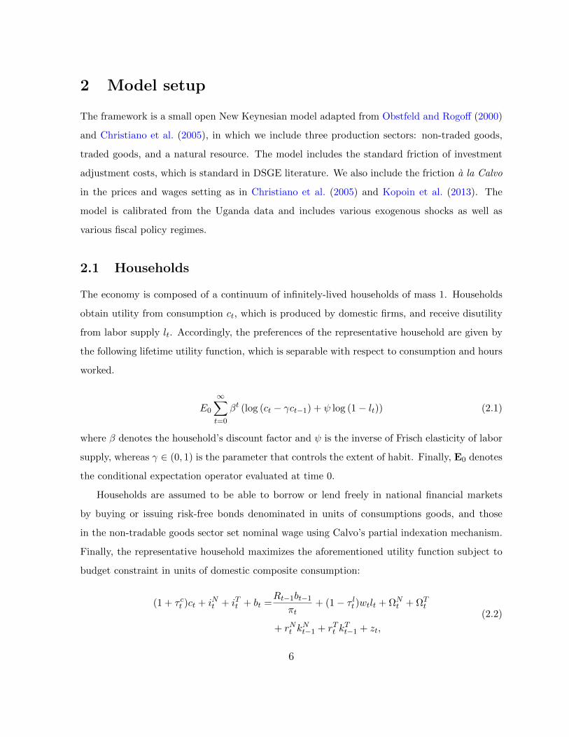
The economy is composed of a continuum of infinitely-lived households of mass 1. Households
obtain utility from consumption ct, which is produced by domestic firms, and receive disutility
from labor supply lt. Accordingly, the preferences of the representative household are given by
the following lifetime utility function, which is separable with respect to consumption and hours
worked.
E0
∞∑t=0
βt (log (ct − γct−1) + ψ log (1− lt)) (2.1)
where β denotes the household’s discount factor and ψ is the inverse of Frisch elasticity of labor
supply, whereas γ ∈ (0, 1) is the parameter that controls the extent of habit. Finally, E0 denotes
the conditional expectation operator evaluated at time 0.
Households are assumed to be able to borrow or lend freely in national financial markets
by buying or issuing risk-free bonds denominated in units of consumptions goods, and those
in the non-tradable goods sector set nominal wage using Calvo’s partial indexation mechanism.
Finally, the representative household maximizes the aforementioned utility function subject to
budget constraint in units of domestic composite consumption:
(1 + τ ct )ct + iNt + iTt + bt =Rt−1bt−1
πt+ (1− τ lt )wtlt + ΩN
t + ΩTt
+ rNt kNt−1 + rTt k
Tt−1 + zt,
(2.2)
6
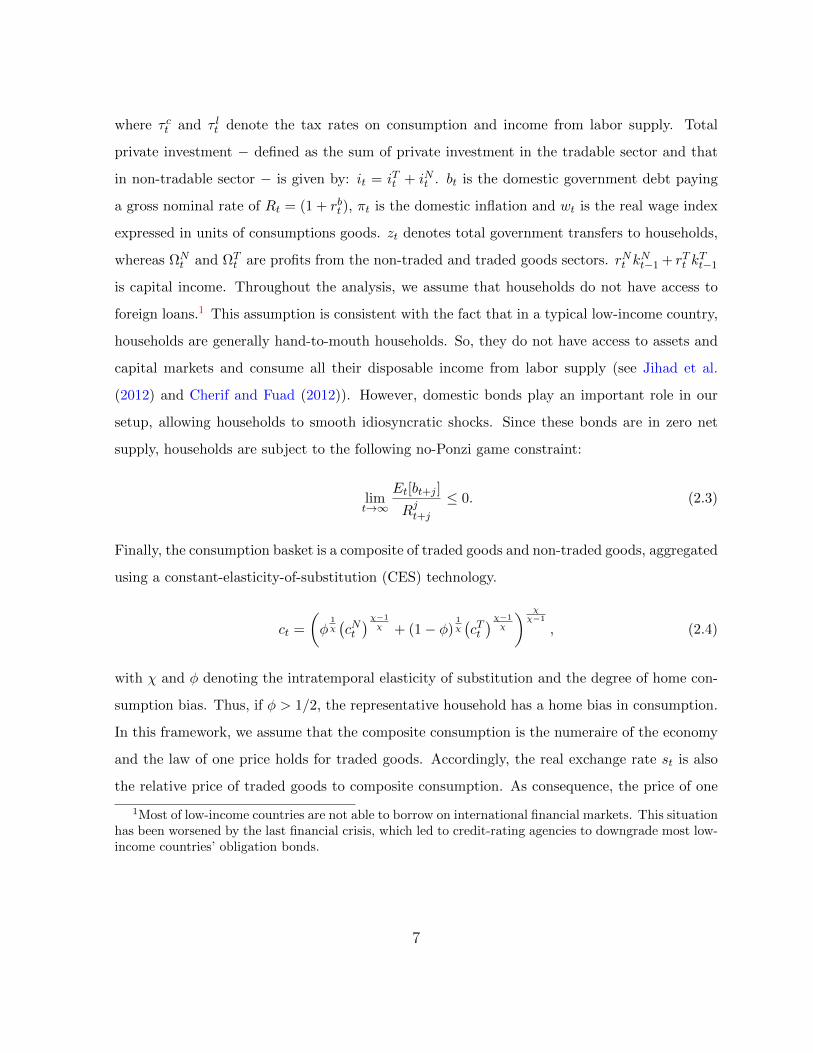
where τ ct and τ lt denote the tax rates on consumption and income from labor supply. Total
private investment − defined as the sum of private investment in the tradable sector and that
in non-tradable sector − is given by: it = iTt + iNt . bt is the domestic government debt paying
a gross nominal rate of Rt = (1 + rbt ), πt is the domestic inflation and wt is the real wage index
expressed in units of consumptions goods. zt denotes total government transfers to households,
whereas ΩNt and ΩT
t are profits from the non-traded and traded goods sectors. rNt kNt−1 + rTt k
Tt−1
is capital income. Throughout the analysis, we assume that households do not have access to
foreign loans.1 This assumption is consistent with the fact that in a typical low-income country,
households are generally hand-to-mouth households. So, they do not have access to assets and
capital markets and consume all their disposable income from labor supply (see Jihad et al.
(2012) and Cherif and Fuad (2012)). However, domestic bonds play an important role in our
setup, allowing households to smooth idiosyncratic shocks. Since these bonds are in zero net
supply, households are subject to the following no-Ponzi game constraint:
limt→∞
Et[bt+j ]
Rjt+j≤ 0. (2.3)
Finally, the consumption basket is a composite of traded goods and non-traded goods, aggregated
using a constant-elasticity-of-substitution (CES) technology.
ct =
(φ
1χ(cNt)χ−1
χ + (1− φ)1χ(cTt)χ−1
χ
) χχ−1
, (2.4)
with χ and φ denoting the intratemporal elasticity of substitution and the degree of home con-
sumption bias. Thus, if φ > 1/2, the representative household has a home bias in consumption.
In this framework, we assume that the composite consumption is the numeraire of the economy
and the law of one price holds for traded goods. Accordingly, the real exchange rate st is also
the relative price of traded goods to composite consumption. As consequence, the price of one
1Most of low-income countries are not able to borrow on international financial markets. This situationhas been worsened by the last financial crisis, which led to credit-rating agencies to downgrade most low-income countries’ obligation bonds.
7
unit of composite consumption is:
1 = φ(pNt)1−χ
+ (1− φ) (st)1−χ . (2.5)
In equation [2.5], pNt denotes the relative price of non-traded goods to composite consumption.
Recall that, non-traded and traded consumption are a composite goods.
cNt =
(∫ 1
0cNt (i)
1− 1χdi
) χχ−1
, and cTt =
(∫ 1
0cTt (i)
1− 1χdi
) χχ−1
. (2.6)
Finally, households supply differentiated labor lt to both traded and non-traded sectors (lNt and
lTt ), and we assume that there is imperfect labor mobility captured by the following constant
elasticity of substitution (CES) function for total labor
lt =
(ω− 1ξ(lNt) 1+ξ
ξ + (1− ω)− 1ξ(lTt) 1+ξ
ξ
) ξ1+ξ
, (2.7)
where ω is the steady-state share of labor supply in the non-traded goods sector, which also
governs labor sectoral mobility in the economy. In equation [2.7], ξ (ξ > 0) is the elasticity of
substitution between the two types of labor. Then, the aggregate real wage index corresponds
to
wt =(ω(wNt)1+ξ
+ (1− ω)(wTt)1+ξ
) 11+ξ
, (2.8)
where wNt and wTt are the real wage rate in the non-traded and traded goods sector, respectively.
Efficient allocation: Given the preferences and the budget constraint, the household’s
optimization problem consists of choosing ct, iNt , iTt , kNt , kTt , and bt for all t ∈ [0,∞) to maximize
lifetime utility function, Ut(·). Finally, given [2.1] and [2.2], households
ψ
1− lt− λt(1− τ l)wt = 0, (2.9)
− λt + βEt
(λt+1
Rt+1
πt+1
)= 0, (2.10)
8
1+ϕN
(kNtkNt−1
− 1
)= βEt
λt+1
λt
1− δN + rNt + ϕN
(kNt+1
kNt− 1
)kNt+1
kNt+ϕN
2
(kNt+1
kNt− 1
)2 ,
(2.11)
1 + ϕT
(kTtkTt−1
− 1
)= βEt
λt+1
λt
1− δT + rTt + ϕT
(kTt+1
kTt− 1
)kTt+1
kTt+ϕT
2
(kTt+1
kTt− 1
)2 .
(2.12)
2.2 Firms
Non-traded good firms are assumed to be monopolistically competitive, while traded good sector
firms are perfectly competitive. In each sector, firms produce goods using labor lt, private
capital (kNt or kTt ) and public capital kGt . In contrast to the natural resource sector, production
and oil prices are assumed to follow exogenous deterministic processes. These assumptions are
consistent and match clearly low-income and small-open economy frameworks since Uganda’s
oil production, as estimated, is relatively small in comparison to world’s oil supply.2 In the
following subsections, we describe the production chain in the tradable and non-tradable goods
sectors.
2.2.1 Non-traded Good Sector
The monopolistic producer i ∈ (0, 1) uses the following technology
yNt = aNt(kNt)αN · (lNt )(1−αN ) ·
(kGt)αG
(2.13)
where aNt is the sectoral total factor productivity (TFP), and kGt−1 is the public capital stock
with an output elasticity of αG. This production technology is well received and documented
in neoclassical literature, featuring public capital as a key input. Following this literature,
Baxter and King (1993) and Kamps (2004) have considered a constant returns to scale function
associated with private inputs (private capital and labor) and an increasing returns to scale
technology, when considering all input factors including public capital. Relative to another
2These assumptions and their quantitative implications are well documented in Ambler et al. (2004),Cherif and Fuad (2012) and Jihad et al. (2012).
9
common specification with constant return to scale to all production factors, this specification
has the advantage that αT and αN can be calibrated to match income shares of labor and private
capital of an economy. Finally, this specification has the advantage to facilitate the steady-state
computation. Private capital evolves by the law of motion
kNt+1 = (1− δN )kNt +
1− ϕN
2
(kNt+1
kNt− 1
)2 iNt︸ ︷︷ ︸
Θ(kNt )
(2.14)
where, Θ(kNt ), is the investment adjustment cost function, satisfying: Θ(1) = Θ′(1) and Θ′′ > 0.3
As in Obstfeld and Rogoff (2000), the monopolistic producer i faces a demand function for the
variety i
yNt (i) =
[pNt (i)
pNt
]yNt , (2.15)
where yNt is the aggregate non-traded demand. A representative non-traded good firm chooses
its price (pNt (i)), labor demand (lNt (i)), and capital stock (kNt+1(i)) to maximize its net present-
value profits, weighted by the household’s marginal utility of consumption (λt).
Et
∞∑t=0
βtλt[(1− ι)pNt (i)yNt (i)− wNt lNt −Adjt(i)− rNt kNt (i) + ιpNt y
Nt
](2.16)
subject to the production function defined in equation [2.13] and the demand function in equation
[2.15]. ι captures distortions in developing countries that discourage firms from investing and
hiring further. ι may be viewed as a distorting tax on firms, but revenue collected remains in
the private sector and is distributed to households and profits. Additionally, this tax helps to
match the relatively low investment to GDP ratios observed in developing countries. However,
this implicit tax is rebated back to the firms as lump-sum transfers.
Denoting by λNt , the Lagrange multiplier associated with the optimization program, which
also may be interpreted as the real marginal cost of producing one unit of output yNt , then the
3Under this specification, the steady-state level of capital stock is not affected by the presence ofadjustment costs.
10
first order conditions of a costs minimizing problem are given by
rNt = λNt αN (1− ι)y
Nt
kNt,
wNt = λNt (1− αN )(1− ι)yNt
lNt,
(2.17)
Price setting: Price rigidity is introduced following a strategy a la Calvo. To this end, we
assume that in each period, a fraction φp of firms cannot change their prices. When allowed to
do so, firm in the non-tradable goods sector chooses the price of its output, pNt (j), in order to
maximize its discounted real profits. All other firms can only index their prices to past inflation
of the composite good price. Indexation is controlled by χp ∈ (0, 1) (χp = 0 refers to a no
indexation case while χp = 1 is a perfect indexation). Intermediate good producer j chooses
the optimal price pNt (j) at the time t. Then, after h periods with no reoptimizing, firm’s price
would evolve over time according to the following recursive equation
pNt+h(j) = (πt+1)χp × (πt+2)χp × · · · × (πt+h−1)χp × pNt (j) =
h−1∏i=1
(πt+i)χppNt (j), (2.18)
where πt+h = pt+h/pt+h−1. The problem of firm j is then:
maxpNt (j)
Et
∞∑i=0
(βφp)lλNt+h
(h−1∏i=1
(πt+i)χp p
Nt (j)
pNt+h−mct+h
)yNt+h(j)
s.c. yNt+h(j) =
(h−1∏i=1
(πt+i)χp p
Nt (j)
pNt+h
)−ξpyNt+h,
(2.19)
where λNt+h is the marginal utility of wealth for a firm j after t + h periods. Assuming that all
firms of type j adopt a same strategy, then the first order condition related to the optimal price
of a domestic intermediate good j is
pNt =ξp
ξp − 1
Et
∞∑i=0
(βφp)hλNt+h
(h−1∏i=1
(πt+i)χp
πt+i+1
)−ξptyNt+h(j)
Et
∞∑i=0
(βφp)lλNt+h
(h−1∏i=1
(πt+i)χp
πt+i+1
)1−ξh,t
yNt+h(j)
, (2.20)
11
In the case of a full indexation (χp = 1), equation [2.20] may be rewritten to derive the New
Keynesian Phillips curve given by: (pNt )1−ξp = φp(pNt−1)1−ξp + (1− φp)(pNt )1−ξp .
Wage setting: Recall that households supply differentiated labor inputs used by interme-
diate good producers and set their nominal wage using Calvo’s partial indexation. We assume
that the aggregate labor is supplied by a representative competitive firm that hires labor sup-
plied by households individually. The differentiated labor inputs supplier aggregates labor using
a constant elasticity of substitution function given by lNt =(∫ 1
0 lNt (i)
ξw−1ξw di
) ξwξw−1
, where ξw
(ξw ∈ (0,∞)) is the elasticity of substitution among different types of labor. The differentiated
labor inputs supplier maximizes profits subject to the production function given all differenti-
ated labor wages, wNt (i), and the aggregate wage, wNt . The first order conditions are such that
lNt (i) =(wNt (i)
wNt
)−ξwlNt and wNt =
(∫ 10 w
Nt (i)1−ξwdi
) 11−ξw . Following Calvo (1983), we include
nominal rigidities on households’ wage setting. Thus, in each period, a fraction 1 − φw can
change their wages, i.e., households only reset optimally the wage contract in states of nature
with a constant probability 1−φw. All others are not able to lay out the optimal wage contract.
In that case, they can only partially index their wages to the past inflation of the composite
domestic goods. The level of indexation is captured by χw ∈ (0, 1). This nominal rigidity implies
that if the household cannot change its wage for h periods, then, its normalized wage is given
byh∏i=1
πχwt+s−1
πt+i
wNt (i)
pt.
Recall that, under the labor supply constraint ( lNt+h(i) =
(∏hi=1
πχwt+h−1
πt+h
wNt (i)
wNt+h
)−ξwlNt+h), the
efficient wage can be written as a geometric average of past real wage and the new optimal wage
in the case of full indexation π1−ξwt
(wNt)1−ξw = φw
(wNt−1
)1−ξw π1−ξwt−1 +(1−φw)π1−ξw
t
(wNt)1−ξw .
2.2.2 Traded Good Sector (Exportable Goods)
I Intermediate tradable good production:
The intermediate traded good sector is perfectly competitive and goods are produced using
12
a similar technology to that in the non-traded good sector.
yiTt = aTt(kTt)αT · (lTt )(1−αT ) ·
(kGt)αG
(2.21)
The total factor productivity (TFP) in the tradable good sector, aTt , is subject to learning-by-
doing externalities, depending on the last period traded output: lnaTt = ρzT lnaTt−1 + d ln yTt−1.
Private capital in the traded good sector also evolves by the law of motion
kTt+1 = (1− δT )kTt +
1− ϕT
2
(kTt+1
kTt− 1
)2 iTt︸ ︷︷ ︸
Θ(kTt )
. (2.22)
Each firm maximizes its weighted present-value profits,
Et
∞∑t=0
βtλTt[(1− ι)styTt (i)− wTt lTt −AdjTt (i)− rTt kTt (i) + ιsty
Tt
](2.23)
Let λTt be the Lagrange multiplier associated with the production function constraint in the
tradable goods sector, which may be interpreted as the real marginal cost of producing one unit
of output yTt . The first order conditions of a minimizing problem are given by
rTt = λTt αT (1− ι)y
iTt
kTt,
wTt = λTt (1− αT )(1− ι)yiTt
lTt,
(2.24)
A part of the intermediate traded good production in the traded goods sector, yTdt , is used for
the domestic market and the remaining part, yTx, is exported in fully competitive market. So
that,
yiTt = yTdt + yTxt . (2.25)
The foreign demand for locally produced goods is as follows:
yTxt =
(pxtp∗t
)−µy∗t , (2.26)
13
where (µ − 1)/µ captures the elasticity of substitution between the exported goods and
foreign-produced goods in the consumption basket of foreign consumers, and y∗t and p∗t are,
respectively, foreign output and the price index. Both variables are exogenously given.
I Final tradable good production:
There is a continuum of intermediate-good-importing firms in a monopolistic competition
market for, which are imperfect substitutes for each other in the production of the composite
imported good, yMt , produced by a representative competitive firm. We also assume Calvo-
type staggered price setting in the imported goods sector to capture the empirical evidence on
incomplete exchange rate pass-through into import prices. The final traded good is produced
by a competitive firm that uses domestically consumed traded goods, yTdt , and imports goods,
yMt following a CES technology
yTt =
(φ
1νm
(yTdt
) ν−1ν
+ (1− φm)1ν(yMt) ν−1
ν
) νν−1
, (2.27)
where φm is the share of domestically consumed traded goods in the final traded goods basket at
the steady state, and ν (ν > 0) is the elasticity of substitution between domestic and imported
goods. The first-order conditions lead to
yTdt = φm
(pdtst
)−νyTt , (2.28)
yMt = (1− φm)
(pMtst
)−νyTt . (2.29)
The final traded good price, pT , which corresponds to the numeraire of our economy is given
by
1 =
[φm
(pdt
)1−ν+ (1− φm)
(pMt)1−ν] 1
1−ν. (2.30)
2.2.3 Natural Resource Sector
Output in the natural resource sector is assumed to follow an exogenous process. This assump-
tion is consistent with the empirical observations since most natural resource production is in
14
reality capital intensive and does not depend on country’s endogenous factors. In addition, most
of resource investments in low-income countries is financed by foreign direct investment (FDI)
that controls the level of oil exploitation. The production function is
ln
(yOtyO
)= ρyo ln
(yOt−1
yO
)+ εyot , (2.31)
where the exogenous process returns to the steady-state level yO with the autoregressive param-
eter ρyo. The resource production shock is assumed to be εyot ∼ i.i.d. and follows a standard
normal distribution with a standard deviation of σyo (εyot ∼ N(0, σ2yo)).
The country’s resource output is assumed relatively small in the world market. Consequently,
Uganda’s resource production is assumed to not be able to affect the international commodity
price pO∗
t . As a result, the international commodity price pO∗
t (relative to the foreign goods)
evolves according to an exogenous process defined by
ln
(pO
∗t
pO∗
)= ρpo ln
(pO
∗t−1
pO∗
)+ εpot , (2.32)
where the international commodity price shock εyot ∼ N(0, σ2yo), and is an i.i.d. process. The
resource GDP from the natural resource sector in units of domestic composite consumption is:
Y Ot = stp
O∗t yOt . (2.33)
As in many resource-rich economies, resource production in Uganda is subject to a royalty at a
rate of τ ot . Thus, the resource revenue collected from the natural resource sector is
TOt = st
(τ ot p
O∗t yOt
)= stT
O∗t . (2.34)
where TO∗t is the resource revenue collected from the natural resource sector expressed in foreign
goods.
15

2.3 Public Sector
The model allows for flexible public policy specifications, and we assume that the public sector
consists of a government and a central bank. In each period, government receives taxes and
contracts domestic debt bt. Total expenditures include government consumption (gCt ), public
investment (gIt ) and debt services. If capital letters denote the aggregate level of a variable, then
government budget constraint may be written as
TOt + τCt Ct + τ ltWtLt +Bt +st(1 + r∗)
π∗tF ∗t−1 = pgtGt +
Rt−1Bt−1
πt+ stF
∗t , (2.35)
where F ∗t is the asset value of resource fund, which generates a constant interest rate r∗. In
[2.36], Gt is government purchases with a relative price to composite consumption goods of pgt .
The model allows external assets accumulation, while we abstracts from external commercial
borrowing. Despite taxing revenues from the non-tradable and tradable goods sectors (ιpNt YNt
and ιstYTt ), the government is unable to use this as an additional source of fiscal revenue.
Consequently, this tax does not appear as revenue in the government’s budget constraint (2.36).
By assuming that they are rebated to the firms, the model captures the inefficiencies of revenue
mobilization in Uganda. Including this feature, our specification makes explicit the challenges
that fiscal authorities in developing economies face regarding tax revenue mobilization. However,
the government collects taxes on revenues from the natural resource sector and they account as
a financing source for public infrastructures.
We define the non-oil fiscal balance that will be used for the fiscal stability measure in the
investigations about the optimal share of oil revenue to be used for public investment as follows:
FBNOt = τCt Ct + τ ltWtLt +Bt − pgtGt −
Rt−1Bt−1
πt. (2.36)
Finally, government purchases consist of expenditures on government consumption GCt and
public investment GI . As in the private consumption, we assume that government purchases
are a CES function of traded and non-traded goods.
Gt =
[η
1χ(GNt)χ−1
χ + (1− η)1χ(GTt)χ−1
χ
] χχ−1
, (2.37)
16
where η is the degree of home bias in government purchases. The relative price of government
consumption to private consumption is
pgt =[η(pNt)1−χ
+ (1− η) (st)1−χ] 1
1−χ. (2.38)
2.3.1 Absorptive Capacity Constraints and Inefficiency of Public Investment
In our framework, we introduce the concept of inefficiency of public investment to capture the
stylized fact of effective public investment in low-income countries by allowing the model to take
into account potential investment inefficiencies and absorptive capacity constraints. As a result,
public investment generates capital accumulation following this law of motion
kGt+1 = (1− δG)kGt + εGGIt , (2.39)
where 0 < (1 − εG) ≤ 1 governs the inefficiency of public investment and δG is the constant
depreciation rate of public capital.
2.3.2 Fiscal Policy
In this framework, we introduce three approaches to analyze fiscal policy in Uganda, which are
different from the use of the fund from the natural resource sector. This involves three regimes of
management of the fiscal policy: the all-investing, the all-saving and the sustainable approaches.
I Policy A: The All-Investing Approach.
Under this approach, the resource fund stays at its initial level, and all additional revenues from
the natural resources sector as well as wage and consumption taxes, and revenues from bonds
issuance are invested in public infrastructures and government consumption. Thus, F ∗t = F ∗,
∀t, while public investment evolves as follows:
GIt = GI +
[TOtpgt− TO
pg
], (2.40)
Gt = GCt +GIt , and (2.41)
17
F ∗t = F ∗, ∀t ∈ [0,∞), (2.42)
where GI , TO and pg are, respectively, the steady state values of GIt , TOt and pgt .
I Policy B: The Saving in a Sovereign Wealth Fund.
Under this fiscal policy, all the resource revenues are saved externally in a sovereign wealth fund
for the future generation. Thus, the resource fund evolves as follows:
F ∗t = F ∗t−1 +
[TOtst− TO
s
](2.43)
Gt = GCt +GIt , and (2.44)
GIt = GI , (2.45)
where s is the steady state values of the real exchange rate.
I Policy C: The Sustainable Investing Approach.
This approach, which may be viewed as a combination of the first two fiscal policies, allows
a constant share of the resource revenues to finance public investment and the remaining part
is saved in a sovereign wealth fund. Under this fiscal policy, the country’s foreign wealth and
public investment are defined as follows:
GIt = GI + φoil[TOtpgt− TO
pg
], (2.46)
Gt = GCt +GIt , and (2.47)
F ∗t = F ∗t−1 + (1− φoil)[TOtst− TO
s
], (2.48)
where φoil is a fiscal policy parameter that satisfies 0 ≤ φoil ≤ 1. At this point, it’s worth
mentioning that the Sustainable Investing Approach and the all-investing approach produce the
same fiscal responses under φoil = 1, and the all-saving approach is obtained by setting φoil = 0.
18
2.3.3 Central Bank
Monetary policy is conducted by the central bank, which manages the short-term nominal
interest rate Rt = (1 + rbt ), in response to fluctuations in domestic output gap and in consumer
price inflation gap using a Taylor-type rule. This managing rule allows the central bank to
smooth nominal interest rates through open market operations.4
log(Rt/R
)= λr log
(Rt−1/R
)+ (1− λr)
(λπlog (πt/π) + λy log
(Yt/Y
))+ ϕt, (2.49)
where Yt denotes the country’s growth domestic product (GDP) and ϕt are i.i.d. normal inno-
vations with a standard deviation of σr.
2.4 Rest of the World
Following the 2014 World Economic Outlook (WEO) released by the IMF, Uganda is considered
as a small open economy. Consequently, a plausible assumption is to assume that domestic
developments do not affect the rest of the world economy. However, the foreign economy’s
dynamics (oil prices) have an impact on the domestic economy. For simplicity, we assume that
the foreign interest rate, foreign output and the world inflation rate are exogenous and follow
AR(1) processes.
2.5 Market Clearing and Competitive Equilibrium
In a competitive equilibrium, the markets for goods, labor and capital all clear. The goods
markets clears when the demand from the agents can be meet by the production of the final
good. To do this, we define real aggregate GDP as the sum of value added in the three sectors,
measured by their steady state prices.
Yt = pNt YNt + stY
T + Y Ot . (2.50)
4The use of the previous period interest rate allows us to match the smooth profile of the observedinterest rate in the data.
19
Then, the general equilibrium in the goods markets involves:
(Ct + It + pGt Gt) + (pxt YTxt − pMt YM
t ) + st(F ∗t − F ∗t−1
)= Yt + str
∗F ∗t−1, (2.51)
where It = INt + ITt is the private investment, and Ct = CNt + CTt is the total consumption.
Recall that government purchases consist of expenditures on government consumption GCt and
public investment GI , therefore Gt = GCt + GIt . Let denote by CAt the current account, then
the balance of payment condition is given by
CAt = pxt YTxt − pMt YM
t + st[(F ∗t − F ∗t−1
)]. (2.52)
Then, labor market clearing requires demand for labor by firms in both sectors to equal the
sector specific supply of labor. This implies that:
Wt ≡∫ 1
0wt(i)di =
∫ 1
0(wNt (i) + wTt (i))di = WN
t +W Tt (2.53)
and
Lt ≡∫ 1
0lt(i)di =
∫ 1
0(lNt (i) + lTt (i))di = LNt + LTt = Ldt , (2.54)
where Ldt denotes total demand for labor by firms in both sectors.
Finally, capital market clearing conditions imply that:
Kt ≡∫ 1
0kt(j)dj =
∫ 1
0(kNt (j) + kTt (i))di = KN
t +KTt , (2.55)
and ∫ 1
0Bt(i)di = 0. (2.56)
2.6 Driving Forces
There are seven sources of uncertainty in our framework: One productivity shock in each of the
two sectors (tradable and non-tradable), an oil price shock that aims to capture the volatility
in the oil price markets, an oil production shock, a foreign demand shock, a foreign price shock
20
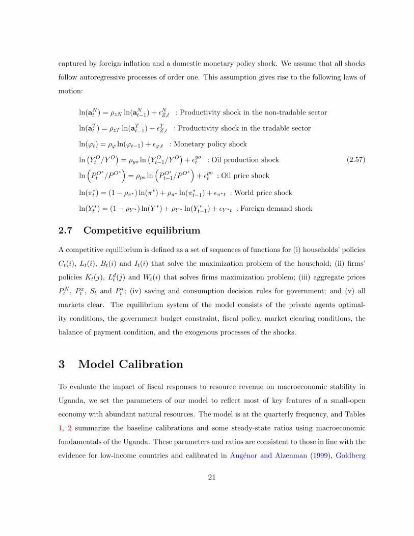
captured by foreign inflation and a domestic monetary policy shock. We assume that all shocks
follow autoregressive processes of order one. This assumption gives rise to the following laws of
motion:
ln(aNt ) = ρzN ln(aNt−1) + εNZ,t : Productivity shock in the non-tradable sector
ln(aTt ) = ρzT ln(aTt−1) + εTZ,t : Productivity shock in the tradable sector
ln(ϕt) = ρϕ ln(ϕt−1) + εϕ,t : Monetary policy shock
ln(Y Ot /Y
O)
= ρyo ln(Y Ot−1/Y
O)
+ εyot : Oil production shock
ln(PO
∗t /PO
∗)
= ρpo ln(PO
∗t−1/P
O∗)
+ εpot : Oil price shock
ln(π∗t ) = (1− ρπ∗) ln(π∗) + ρπ∗ ln(π∗t−1) + επ∗t : World price shock
ln(Y ∗t ) = (1− ρY ∗) ln(Y ∗) + ρY ∗ ln(Y ∗t−1) + εY ∗t : Foreign demand shock
(2.57)
2.7 Competitive equilibrium
A competitive equilibrium is defined as a set of sequences of functions for (i) households’ policies
Ct(i), Lt(i), Bt(i) and It(i) that solve the maximization problem of the household; (ii) firms’
policies Kt(j), Ldt (j) and Wt(i) that solves firms maximization problem; (iii) aggregate prices
PNt , P xt , St and P ∗t ; (iv) saving and consumption decision rules for government; and (v) all
markets clear. The equilibrium system of the model consists of the private agents optimal-
ity conditions, the government budget constraint, fiscal policy, market clearing conditions, the
balance of payment condition, and the exogenous processes of the shocks.
3 Model Calibration
To evaluate the impact of fiscal responses to resource revenue on macroeconomic stability in
Uganda, we set the parameters of our model to reflect most of key features of a small-open
economy with abundant natural resources. The model is at the quarterly frequency, and Tables
1, 2 summarize the baseline calibrations and some steady-state ratios using macroeconomic
fundamentals of the Uganda. These parameters and ratios are consistent to those in line with the
evidence for low-income countries and calibrated in Angenor and Aizenman (1999), Goldberg
21
(2011) and Agenor (2014). Data sources used to match key ratios include the IMF’s World
Economic Outlook (WEO) database, the oil and revenue management policy framework provided
by the Uganda’s Ministry of Finance and various research papers such as Pritchett (2000),
Goldberg (2011), Angenor and Aizenman (1999), Kopoin et al. (2013) and Agenor (2014).
In the representative household’s utility function, the weight on leisure ψ is set to 3, which
leads to the steady-state value of household work effort to be 40 percent of available time. The
household’s discount factor, β, is set 0.93, implying a long-run real interest rate of 9.68 percent
annually. This assumption is fairly reasonable and consistent regarding banks’ interest rates in
most of low-income countries (see African Development Indicators (ADI)). In addition, the share
of capital in the production function for intermediate goods in the non-traded goods sector, αN ,
is set to 0.45, while it is set to 0.3 in the traded goods sector. These values indicate that the
informal (non-tradable goods sector) sector is more intensive in labor than the tradable goods
sector. The depreciation rates of capital are fixed to 0.1 in the informal sector and 0.075 in
the tradable goods sector. All these values are consistent with studies on Sub-Saharan African
countries and reported in Jihad et al. (2012), Cherif and Fuad (2012) and Agenor (2014).
In our paper, we use the empirical evidence based on Mexican data from 1980 to 1994 by
Arestoff and Hurlin (2006) to pin-down the parameter that governs the efficiency of public invest-
ment εG. This paper shows that the coefficient of regressing public capital produced (effective
investment in our model) on investment expenditures falls between 0.4 and 0.65. This range of
investment efficiency is in line with the estimates in Pritchett (2000) for Sub-Saharan African
countries with a linear specification between effective investment and investment expenditures.
Based on these empirical papers and the macroeconomic efforts undertaken by the government
to sustain public investment, we set εG to 0.6.
The nominal price rigidity parameter in the non-traded goods sector, as well as the nominal
wage-setting parameter are set following Calvo’s model of staggered price and wage adjustment.
As in Christiano et al. (2005), the probability of not reoptimizing for price and wage setters in
the domestic country, φp and φw, are fixed to 0.75 and 0.64, respectively. The degree of home
bias in private consumption, φ, and the elasticity of substitution between domestic labor types,
ξ, are set to 0.4 and 1, respectively. These values are estimated in Christiano et al. (2010) for
22
the U.S. economy and are commonly used in the literature of developing countries.
The domestic monetary policy parameters λr, λπ et λy are set to 0.8, 1.5 and 0.1/4, respec-
tively. These values satisfy the Taylor principle and are consistent to those estimated in Agenor
(2014) and Kopoin et al. (2013). The standard deviation of both domestic and foreign mone-
tary policy shocks is fixed to 0.0016, ρmp = ρRf = 0.0016, which ensures that a one-standard
deviation shock moves the interest rate by 0.6 percentage points. This value is consistent to the
empirical estimates reported in Christiano et al. (2005).
The model is solved using a second-order perturbation method around its deterministic
steady state.
4 Findings
The patterns of investment and saving out of income from the oil windfall in managing of the
optimal fiscal policy remain ambiguous for policymakers. In practice, the key issue for the
spending of oil revenue by the government, viewed as a Ramsey problem, is to scale up public
investment to meet huge needs in public infrastructure without generating higher public sector
deficits and a Dutch disease in an uncertain oil production world, characterized by unexpected
shocks and prices volatility. To address this issue with our baseline DSGE model, we simulate
the effects of oil production shocks and interpret it as a boom in the oil sector. Using the
parameters calibrated to reflect the key features of a small open economy such as Uganda, we
focus on the impulse response functions of some key variables. Throughout, we simulate and
compare the impulse responses to a one standard-deviation shock to the oil production.
Figures 1, 2 and 3 show impulse responses by illustrating macroeconomic dynamics under
three stylized fiscal policy approaches for managing a resource windfall: investing in public
capital, saving in a sovereign wealth and sustainable investing in public capital. In Table 1, the
solid lines present the responses under the fiscal policy A (investing in public capital), and the
dashed lines are under the fiscal policy B (saving in a sovereign wealth fund). Solid lines in
Figure 3 remain the responses under the fiscal policy A, while dashed lines present responses
23
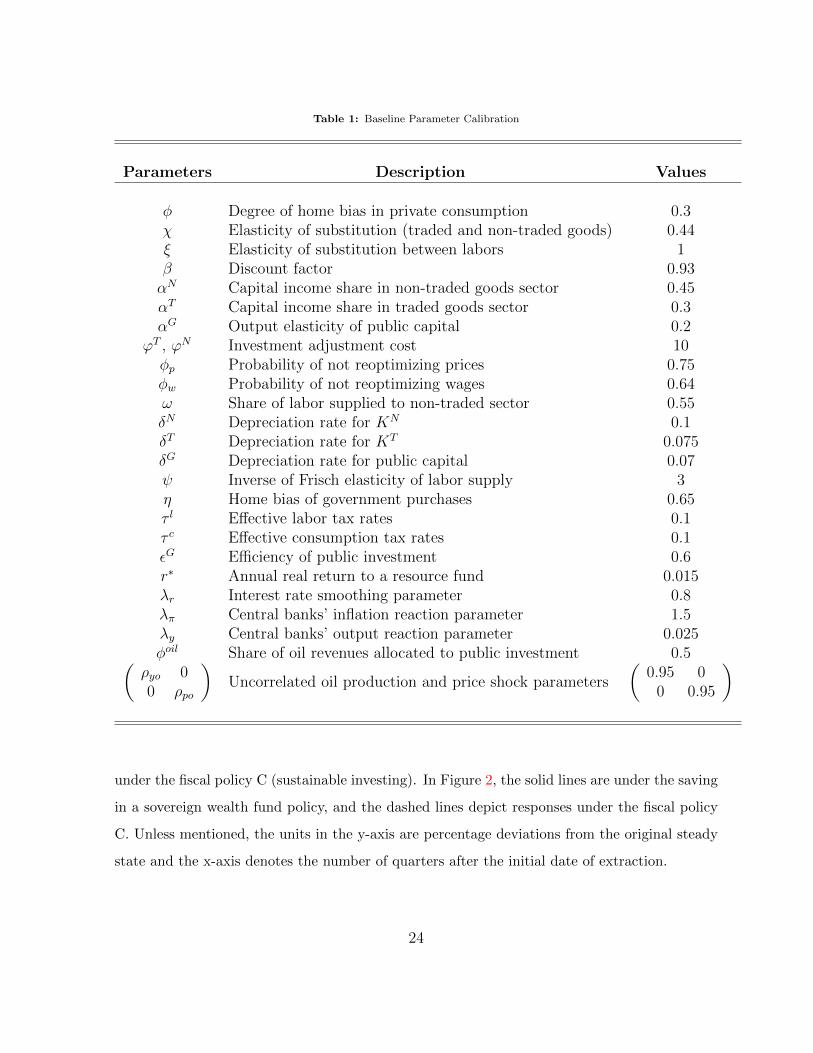
Table 1: Baseline Parameter Calibration
Parameters Description Values
φ Degree of home bias in private consumption 0.3χ Elasticity of substitution (traded and non-traded goods) 0.44ξ Elasticity of substitution between labors 1β Discount factor 0.93αN Capital income share in non-traded goods sector 0.45αT Capital income share in traded goods sector 0.3αG Output elasticity of public capital 0.2
ϕT , ϕN Investment adjustment cost 10φp Probability of not reoptimizing prices 0.75φw Probability of not reoptimizing wages 0.64ω Share of labor supplied to non-traded sector 0.55δN Depreciation rate for KN 0.1δT Depreciation rate for KT 0.075δG Depreciation rate for public capital 0.07ψ Inverse of Frisch elasticity of labor supply 3η Home bias of government purchases 0.65τ l Effective labor tax rates 0.1τ c Effective consumption tax rates 0.1εG Efficiency of public investment 0.6r∗ Annual real return to a resource fund 0.015λr Interest rate smoothing parameter 0.8λπ Central banks’ inflation reaction parameter 1.5λy Central banks’ output reaction parameter 0.025φoil Share of oil revenues allocated to public investment 0.5(
ρyo 00 ρpo
)Uncorrelated oil production and price shock parameters
(0.95 0
0 0.95
)
under the fiscal policy C (sustainable investing). In Figure 2, the solid lines are under the saving
in a sovereign wealth fund policy, and the dashed lines depict responses under the fiscal policy
C. Unless mentioned, the units in the y-axis are percentage deviations from the original steady
state and the x-axis denotes the number of quarters after the initial date of extraction.
24
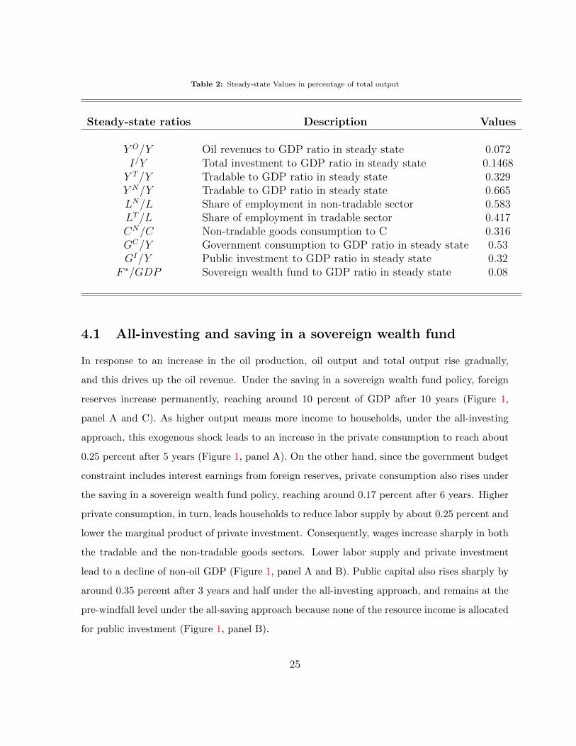
Table 2: Steady-state Values in percentage of total output
Steady-state ratios Description Values
Y O/Y Oil revenues to GDP ratio in steady state 0.072I/Y Total investment to GDP ratio in steady state 0.1468Y T/Y Tradable to GDP ratio in steady state 0.329Y N/Y Tradable to GDP ratio in steady state 0.665LN/L Share of employment in non-tradable sector 0.583LT/L Share of employment in tradable sector 0.417CN/C Non-tradable goods consumption to C 0.316GC/Y Government consumption to GDP ratio in steady state 0.53GI/Y Public investment to GDP ratio in steady state 0.32
F ∗/GDP Sovereign wealth fund to GDP ratio in steady state 0.08
4.1 All-investing and saving in a sovereign wealth fund
In response to an increase in the oil production, oil output and total output rise gradually,
and this drives up the oil revenue. Under the saving in a sovereign wealth fund policy, foreign
reserves increase permanently, reaching around 10 percent of GDP after 10 years (Figure 1,
panel A and C). As higher output means more income to households, under the all-investing
approach, this exogenous shock leads to an increase in the private consumption to reach about
0.25 percent after 5 years (Figure 1, panel A). On the other hand, since the government budget
constraint includes interest earnings from foreign reserves, private consumption also rises under
the saving in a sovereign wealth fund policy, reaching around 0.17 percent after 6 years. Higher
private consumption, in turn, leads households to reduce labor supply by about 0.25 percent and
lower the marginal product of private investment. Consequently, wages increase sharply in both
the tradable and the non-tradable goods sectors. Lower labor supply and private investment
lead to a decline of non-oil GDP (Figure 1, panel A and B). Public capital also rises sharply by
around 0.35 percent after 3 years and half under the all-investing approach, and remains at the
pre-windfall level under the all-saving approach because none of the resource income is allocated
for public investment (Figure 1, panel B).
25
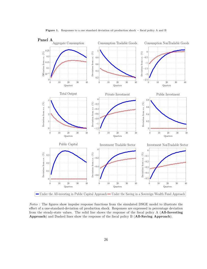
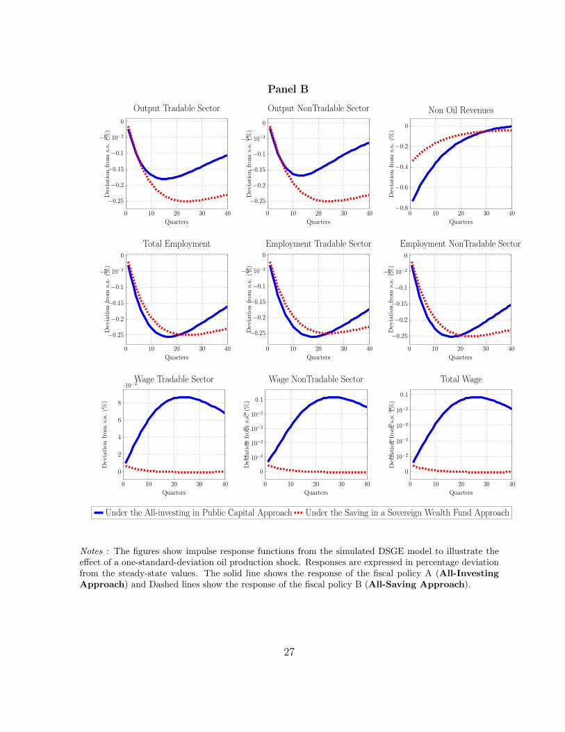
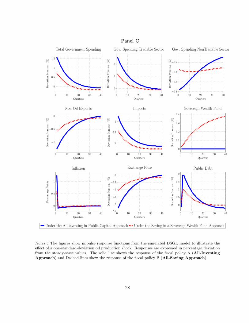
Figure 1. Responses to a one standard deviation oil production shock − fiscal policy A and B
7 Simulated results
Table 3: Responses to a one standard deviation oil production shock − fiscal policy A and B
Panel A
0 10 20 30 400
5 · 10−2
0.1
0.15
0.2
0.25
Quarters
Dev
iati
on
from
s.s.
(%)
Aggregate Consumption
0 10 20 30 40
0.2
0.4
0.6
0.8
1
Quarters
Dev
iati
on
from
s.s.
(%)
Consumption Tradable Goods
0 10 20 30 40−2.5
−2
−1.5
−1
−0.5
0
Quarters
Dev
iati
on
from
s.s.
(%)
Consumption NonTradable Goods
0 10 20 30 40
0
1
2
3
4
Quarters
Dev
iati
on
from
s.s.
(%)
Total Output
0 10 20 30 40
−1.2
−1
−0.8
−0.6
−0.4
−0.2
0
Quarters
Dev
iati
on
from
s.s.
(%)
Private Investment
0 10 20 30 40
0
0.2
0.4
0.6
0.8
Quarters
Dev
iati
on
from
s.s.
(%)
Public Investment
0 10 20 30 40
0
0.1
0.2
0.3
Quarters
Dev
iati
on
from
s.s.
(%)
Public Capital
0 10 20 30 40
−0.6
−0.4
−0.2
0
Quarters
Dev
iati
on
from
s.s.
(%)
Investment Tradable Sector
0 10 20 30 40
−0.5
−0.4
−0.3
−0.2
−0.1
0
Quarters
Dev
iati
on
from
s.s.
(%)
Investment NonTradable Sector
Under the All-investing in Public Capital Approach Under the Saving in a Sovereign Wealth Fund Approach
Notes : The figures show impulse response functions from the simulated DSGE model toillustrate the effect of a one-standard-deviation oil production shock. Responses are
expressed in percentage deviation from the steady-state values. The solid line shows theresponse of the fiscal policy A (All-Investing Approach) and Dashed lines show the
response of the fiscal policy B (All-Saving Approach).
49
Notes : The figures show impulse response functions from the simulated DSGE model to illustrate theeffect of a one-standard-deviation oil production shock. Responses are expressed in percentage deviationfrom the steady-state values. The solid line shows the response of the fiscal policy A (All-InvestingApproach) and Dashed lines show the response of the fiscal policy B (All-Saving Approach).
26
Panel B
0 10 20 30 40
−0.25
−0.2
−0.15
−0.1
−5 · 10−2
0
Quarters
Dev
iati
on
from
s.s.
(%)
Output Tradable Sector
0 10 20 30 40
−0.25
−0.2
−0.15
−0.1
−5 · 10−2
0
Quarters
Dev
iati
on
from
s.s.
(%)
Output NonTradable Sector
0 10 20 30 40−0.8
−0.6
−0.4
−0.2
0
Quarters
Dev
iati
on
from
s.s.
(%)
Non Oil Revenues
0 10 20 30 40
−0.25
−0.2
−0.15
−0.1
−5 · 10−2
0
Quarters
Dev
iati
on
from
s.s.
(%)
Total Employment
0 10 20 30 40
−0.25
−0.2
−0.15
−0.1
−5 · 10−2
0
Quarters
Dev
iati
on
from
s.s.
(%)
Employment Tradable Sector
0 10 20 30 40
−0.25
−0.2
−0.15
−0.1
−5 · 10−2
0
Quarters
Dev
iati
on
from
s.s.
(%)
Employment NonTradable Sector
0 10 20 30 40
0
2
4
6
8
·10−2
Quarters
Dev
iati
on
from
s.s.
(%)
Wage Tradable Sector
0 10 20 30 40
0
2 · 10−2
4 · 10−2
6 · 10−2
8 · 10−2
0.1
Quarters
Dev
iati
on
from
s.s.
(%)
Wage NonTradable Sector
0 10 20 30 40
0
2 · 10−2
4 · 10−2
6 · 10−2
8 · 10−2
0.1
Quarters
Dev
iati
on
from
s.s.
(%)
Total Wage
Under the All-investing in Public Capital Approach Under the Saving in a Sovereign Wealth Fund Approach
Notes : The figures show impulse response functions from the simulated DSGE model toillustrate the effect of a one-standard-deviation oil production shock. Responses are
expressed in percentage deviation from the steady-state values. The solid line shows theresponse of the fiscal policy A (All-Investing Approach) and Dashed lines show the
response of the fiscal policy B (All-Saving Approach).
50
Notes : The figures show impulse response functions from the simulated DSGE model to illustrate theeffect of a one-standard-deviation oil production shock. Responses are expressed in percentage deviationfrom the steady-state values. The solid line shows the response of the fiscal policy A (All-InvestingApproach) and Dashed lines show the response of the fiscal policy B (All-Saving Approach).
27
Panel C
0 10 20 30 40
0
0.5
1
1.5
Quarters
Dev
iati
on
from
s.s.
(%)
Total Government Spending
0 10 20 30 40
0
1
2
Quarters
Dev
iati
on
from
s.s.
(%)
Gov. Spending Tradable Sector
0 10 20 30 40−0.8
−0.6
−0.4
−0.2
Quarters
Dev
iati
on
from
s.s.
(%)
Gov. Spending NonTradable Sector
0 10 20 30 40
−1
−0.5
0
Quarters
Dev
iati
on
from
s.s.
(%)
Non Oil Exports
0 10 20 30 40
0
0.5
1
Quarters
Dev
iati
on
from
s.s.
(%)
Imports
0 10 20 30 40
0
0.1
0.2
0.3
0.4
Quarters
Dev
iati
on
from
s.s.
(%)
Sovereign Wealth Fund
0 10 20 30 40
0
0.5
1
Quarters
Per
centa
ge
Poin
ts
Inflation
0 10 20 30 40−2.5
−2
−1.5
−1
−0.5
0
Quarters
Dev
iati
on
from
s.s.
(%)
Exchange Rate
0 10 20 30 40
0
0.5
1
1.5
2
Quarters
Dev
iati
on
from
s.s.
(%)
Public Debt
Under the All-investing in Public Capital Approach Under the Saving in a Sovereign Wealth Fund Approach
Notes : The figures show impulse response functions from the simulated DSGE model toillustrate the effect of a one-standard-deviation oil production shock. Responses are
expressed in percentage deviation from the steady-state values. The solid line shows theresponse of the fiscal policy A (All-Investing Approach) and Dashed lines show the
response of the fiscal policy B (All-Saving Approach).
51
Notes : The figures show impulse response functions from the simulated DSGE model to illustrate theeffect of a one-standard-deviation oil production shock. Responses are expressed in percentage deviationfrom the steady-state values. The solid line shows the response of the fiscal policy A (All-InvestingApproach) and Dashed lines show the response of the fiscal policy B (All-Saving Approach).
28
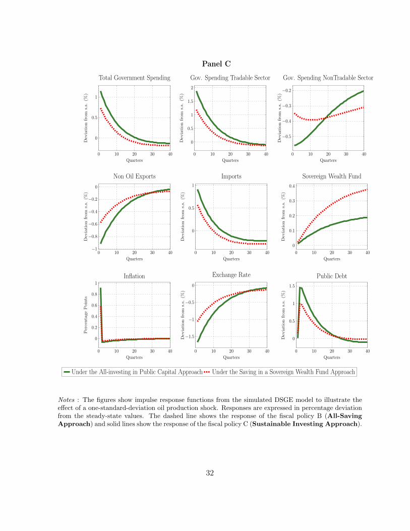
A boom in the oil sector makes the country a net exporter. Then, the wealth and income
accumulated from the resource windfall increase, generating more revenue for government. As
a result, demand in the non-tradable goods sector increases, leading to a substantial rise in
the prices of non-tradable goods. Since Uganda is considered as a small open economy and
a price taker in the international tradable goods market, the real exchange rate, defined as
the relative price of non-tradable to tradable, appreciates consequently. This appreciation,
which is more pronounced under the all-investing approach, reduces the competitiveness of
the country’s exports and domestic imports-competing products. Therefore, imports become
relatively cheaper, leading to a rise in the total imports by about 1.2 percent and a fall of non-
oil exports by around 1.3 percent (Figure 1, panel C). Finally, under the all-saving approach,
the economy experiences smaller movements because resource income is directly saved into
a foreign account. In contrast, under the all-investing approach, the oil production shock is
more persistent and the return to the pre-windfall equilibrium is done more slowly. Comparing
these two stylized fiscal policies, simulations show that the boom in the oil production sector
generates sizeable macroeconomic activity under the all-investing approach. However, the all-
saving approach is much less susceptible to generate Dutch disease effects.
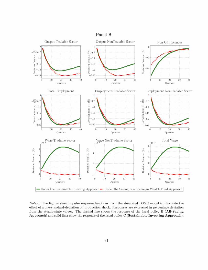
4.2 The sustainable investing approach
In this subsection, we compare the first two fiscal approaches to the sustainable investing ap-
proach. This latter fiscal policy, which may be viewed as a mixed policy, can conciliate public
investment and saving approach by proposing a new investment with external saving approach.
We allow the government to use half of the oil revenue for public investment (φoil = 0.5) and to
save the remaining half; Section 4.4 investigates the optimal value of φoil. As described in 2.48,
this new approach allows policymakers to choose an optimal scaling up magnitude given the size
of the oil production and economic characteristics. Figures 2 and 3 show impulse responses of
the main macroeconomic aggregates in comparison with the first two fiscal policy approaches.
Under the three stylized fiscal policies, simulations show that the boom in the oil sector leads
to deteriorate employment in both the tradable and non-tradable goods sectors. This result,
which might be surprising, is resulting from two macroeconomic effects: substitution and wealth
29
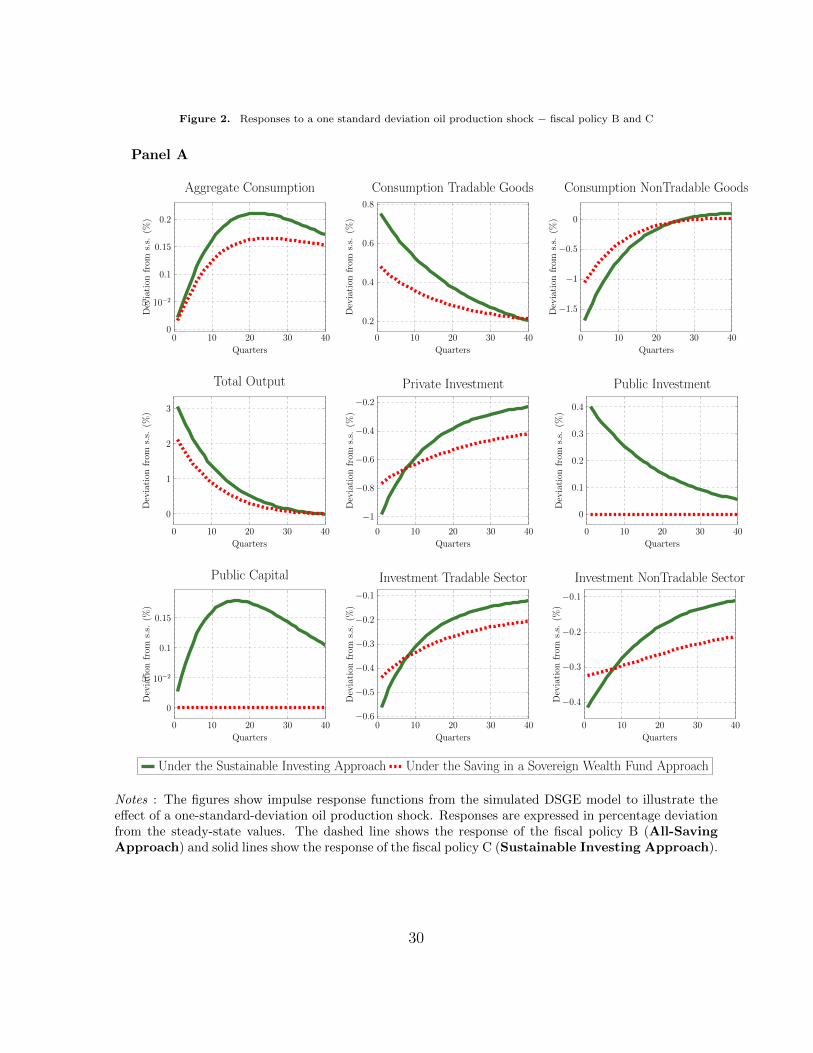
Figure 2. Responses to a one standard deviation oil production shock − fiscal policy B and CTable 4: Responses to a one standard deviation oil production shock − fiscal policy B and C
Panel A
0 10 20 30 400
5 · 10−2
0.1
0.15
0.2
Quarters
Dev
iati
on
from
s.s.
(%)
Aggregate Consumption
0 10 20 30 40
0.2
0.4
0.6
0.8
QuartersD
evia
tion
from
s.s.
(%)
Consumption Tradable Goods
0 10 20 30 40
−1.5
−1
−0.5
0
Quarters
Dev
iati
on
from
s.s.
(%)
Consumption NonTradable Goods
0 10 20 30 40
0
1
2
3
Quarters
Dev
iati
on
from
s.s.
(%)
Total Output
0 10 20 30 40
−1
−0.8
−0.6
−0.4
−0.2
Quarters
Dev
iati
on
from
s.s.
(%)
Private Investment
0 10 20 30 40
0
0.1
0.2
0.3
0.4
Quarters
Dev
iati
on
from
s.s.
(%)
Public Investment
0 10 20 30 40
0
5 · 10−2
0.1
0.15
Quarters
Dev
iati
on
from
s.s.
(%)
Public Capital
0 10 20 30 40−0.6
−0.5
−0.4
−0.3
−0.2
−0.1
Quarters
Dev
iati
on
from
s.s.
(%)
Investment Tradable Sector
0 10 20 30 40
−0.4
−0.3
−0.2
−0.1
Quarters
Dev
iati
on
from
s.s.
(%)
Investment NonTradable Sector
Under the Sustainable Investing Approach Under the Saving in a Sovereign Wealth Fund Approach
Notes : The figures show impulse response functions from the simulated DSGE model toillustrate the effect of a one-standard-deviation oil production shock. Responses are
expressed in percentage deviation from the steady-state values. The dashed line showsthe response of the fiscal policy B (All-Saving Approach) and solid lines show the
response of the fiscal policy C (Sustainable Investing Approach).
52
Notes : The figures show impulse response functions from the simulated DSGE model to illustrate theeffect of a one-standard-deviation oil production shock. Responses are expressed in percentage deviationfrom the steady-state values. The dashed line shows the response of the fiscal policy B (All-SavingApproach) and solid lines show the response of the fiscal policy C (Sustainable Investing Approach).
30
Panel B
0 10 20 30 40
−0.25
−0.2
−0.15
−0.1
−5 · 10−2
0
Quarters
Dev
iati
onfr
oms.
s.(%
)
Output Tradable Sector
0 10 20 30 40
−0.25
−0.2
−0.15
−0.1
−5 · 10−2
0
Quarters
Dev
iati
onfr
oms.
s.(%
)
Output NonTradable Sector
0 10 20 30 40
−0.4
−0.2
0
Quarters
Dev
iati
onfr
oms.
s.(%
)
Non Oil Revenues
0 10 20 30 40
−0.25
−0.2
−0.15
−0.1
−5 · 10−2
0
Quarters
Dev
iati
onfr
oms.
s.(%
)
Total Employment
0 10 20 30 40
−0.25
−0.2
−0.15
−0.1
−5 · 10−2
0
Quarters
Dev
iati
onfr
oms.
s.(%
)Employment Tradable Sector
0 10 20 30 40
−0.25
−0.2
−0.15
−0.1
−5 · 10−2
0
Quarters
Dev
iati
onfr
oms.
s.(%
)
Employment NonTradable Sector
0 10 20 30 40
0
1
2
3
4
·10−2
Quarters
Dev
iati
onfr
oms.
s.(%
)
Wage Tradable Sector
0 10 20 30 40
0
2
4
·10−2
Quarters
Dev
iati
onfr
oms.
s.(%
)
Wage NonTradable Sector
0 10 20 30 40
0
1
2
3
4
5
·10−2
Quarters
Dev
iati
onfr
oms.
s.(%
)Total Wage
Under the Sustainable Investing Approach Under the Saving in a Sovereign Wealth Fund Approach
Notes : The figures show impulse response functions from the simulated DSGE model toillustrate the effect of a one-standard-deviation oil production shock. Responses are
expressed in percentage deviation from the steady-state values. The dashed line showsthe response of the fiscal policy B (All-Saving Approach) and solid lines show the
response of the fiscal policy C (Sustainable Investing Approach).
53
Notes : The figures show impulse response functions from the simulated DSGE model to illustrate theeffect of a one-standard-deviation oil production shock. Responses are expressed in percentage deviationfrom the steady-state values. The dashed line shows the response of the fiscal policy B (All-SavingApproach) and solid lines show the response of the fiscal policy C (Sustainable Investing Approach).
31
Panel C
0 10 20 30 40
0
0.5
1
Quarters
Dev
iati
on
from
s.s.
(%)
Total Government Spending
0 10 20 30 40
0
0.5
1
1.5
2
Quarters
Dev
iati
on
from
s.s.
(%)
Gov. Spending Tradable Sector
0 10 20 30 40
−0.5
−0.4
−0.3
−0.2
Quarters
Dev
iati
on
from
s.s.
(%)
Gov. Spending NonTradable Sector
0 10 20 30 40−1
−0.8
−0.6
−0.4
−0.2
0
Quarters
Dev
iati
on
from
s.s.
(%)
Non Oil Exports
0 10 20 30 40
0
0.5
1
Quarters
Dev
iati
on
from
s.s.
(%)
Imports
0 10 20 30 40
0
0.1
0.2
0.3
0.4
Quarters
Dev
iati
on
from
s.s.
(%)
Sovereign Wealth Fund
0 10 20 30 40
0
0.2
0.4
0.6
0.8
1
Quarters
Per
centa
ge
Poin
ts
Inflation
0 10 20 30 40
−1.5
−1
−0.5
0
Quarters
Dev
iati
on
from
s.s.
(%)
Exchange Rate
0 10 20 30 40
0
0.5
1
1.5
Quarters
Dev
iati
on
from
s.s.
(%)
Public Debt
Under the All-investing in Public Capital Approach Under the Saving in a Sovereign Wealth Fund Approach
Notes : The figures show impulse response functions from the simulated DSGE model toillustrate the effect of a one-standard-deviation oil production shock. Responses are
expressed in percentage deviation from the steady-state values. The dashed line showsthe response of the fiscal policy B (All-Saving Approach) and solid lines show the
response of the fiscal policy C (Sustainable Investing Approach).
54
Notes : The figures show impulse response functions from the simulated DSGE model to illustrate theeffect of a one-standard-deviation oil production shock. Responses are expressed in percentage deviationfrom the steady-state values. The dashed line shows the response of the fiscal policy B (All-SavingApproach) and solid lines show the response of the fiscal policy C (Sustainable Investing Approach).
32
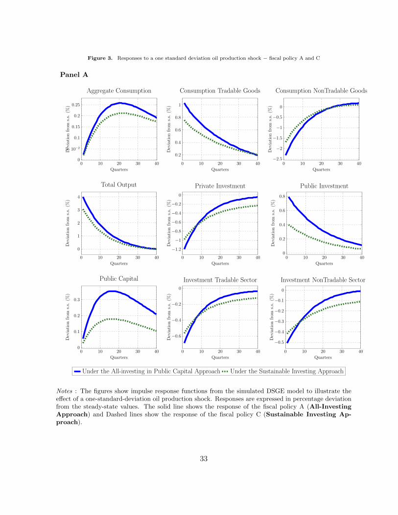
Figure 3. Responses to a one standard deviation oil production shock − fiscal policy A and CTable 5: Responses to a one standard deviation oil production shock − fiscal policy A and C
Panel A
0 10 20 30 400
5 · 10−2
0.1
0.15
0.2
0.25
Quarters
Dev
iati
onfr
oms.
s.(%
)
Aggregate Consumption
0 10 20 30 40
0.2
0.4
0.6
0.8
1
QuartersD
evia
tion
from
s.s.
(%)
Consumption Tradable Goods
0 10 20 30 40−2.5
−2
−1.5
−1
−0.5
0
Quarters
Dev
iati
onfr
oms.
s.(%
)
Consumption NonTradable Goods
0 10 20 30 40
0
1
2
3
4
Quarters
Dev
iati
onfr
oms.
s.(%
)
Total Output
0 10 20 30 40
−1.2
−1
−0.8
−0.6
−0.4
−0.2
0
Quarters
Dev
iati
onfr
oms.
s.(%
)
Private Investment
0 10 20 30 400
0.2
0.4
0.6
0.8
Quarters
Dev
iati
onfr
oms.
s.(%
)
Public Investment
0 10 20 30 400
0.1
0.2
0.3
Quarters
Dev
iati
onfr
oms.
s.(%
)
Public Capital
0 10 20 30 40
−0.6
−0.4
−0.2
0
Quarters
Dev
iati
onfr
oms.
s.(%
)
Investment Tradable Sector
0 10 20 30 40
−0.5
−0.4
−0.3
−0.2
−0.1
0
Quarters
Dev
iati
onfr
oms.
s.(%
)
Investment NonTradable Sector
Under the All-investing in Public Capital Approach Under the Sustainable Investing Approach
Notes : The figures show impulse response functions from the simulated DSGE model toillustrate the effect of a one-standard-deviation oil production shock. Responses are
expressed in percentage deviation from the steady-state values. The solid line shows theresponse of the fiscal policy A (All-Investing Approach) and Dashed lines show the
response of the fiscal policy C (Sustainable Investing Approach).
55
Notes : The figures show impulse response functions from the simulated DSGE model to illustrate theeffect of a one-standard-deviation oil production shock. Responses are expressed in percentage deviationfrom the steady-state values. The solid line shows the response of the fiscal policy A (All-InvestingApproach) and Dashed lines show the response of the fiscal policy C (Sustainable Investing Ap-proach).
33
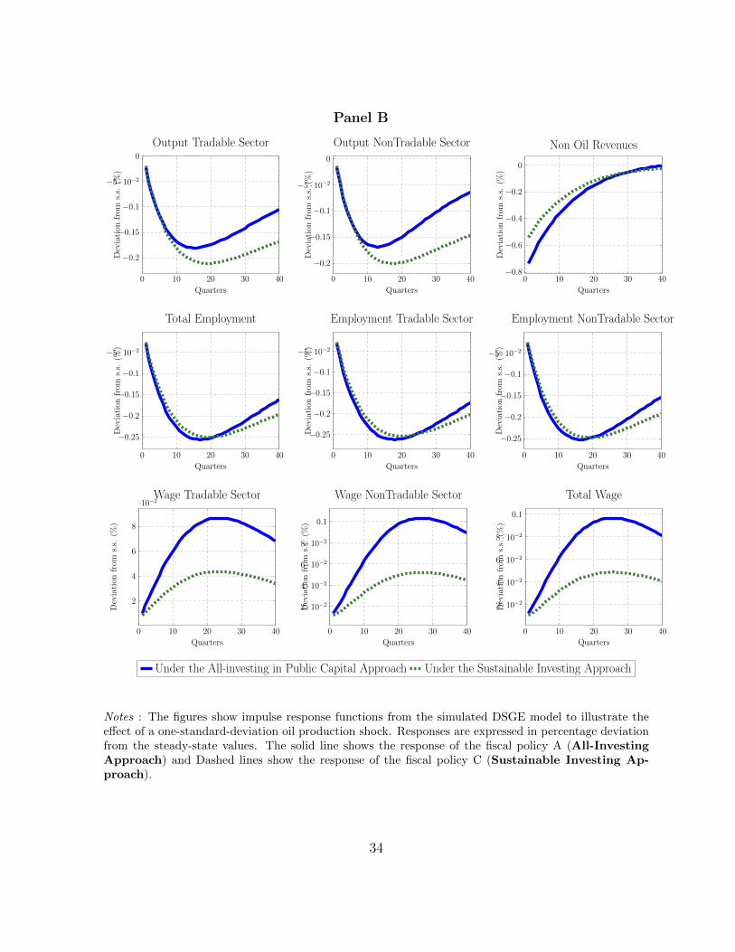
Panel B
0 10 20 30 40
−0.2
−0.15
−0.1
−5 · 10−2
0
Quarters
Dev
iati
on
from
s.s.
(%)
Output Tradable Sector
0 10 20 30 40
−0.2
−0.15
−0.1
−5 · 10−2
0
Quarters
Dev
iati
on
from
s.s.
(%)
Output NonTradable Sector
0 10 20 30 40−0.8
−0.6
−0.4
−0.2
0
Quarters
Dev
iati
on
from
s.s.
(%)
Non Oil Revenues
0 10 20 30 40
−0.25
−0.2
−0.15
−0.1
−5 · 10−2
Quarters
Dev
iati
on
from
s.s.
(%)
Total Employment
0 10 20 30 40
−0.25
−0.2
−0.15
−0.1
−5 · 10−2
Quarters
Dev
iati
on
from
s.s.
(%)
Employment Tradable Sector
0 10 20 30 40
−0.25
−0.2
−0.15
−0.1
−5 · 10−2
Quarters
Dev
iati
on
from
s.s.
(%)
Employment NonTradable Sector
0 10 20 30 40
2
4
6
8
·10−2
Quarters
Dev
iati
on
from
s.s.
(%)
Wage Tradable Sector
0 10 20 30 40
2 · 10−2
4 · 10−2
6 · 10−2
8 · 10−2
0.1
Quarters
Dev
iati
on
from
s.s.
(%)
Wage NonTradable Sector
0 10 20 30 40
2 · 10−2
4 · 10−2
6 · 10−2
8 · 10−2
0.1
Quarters
Dev
iati
on
from
s.s.
(%)
Total Wage
Under the All-investing in Public Capital Approach Under the Sustainable Investing Approach
Notes : The figures show impulse response functions from the simulated DSGE model toillustrate the effect of a one-standard-deviation oil production shock. Responses are
expressed in percentage deviation from the steady-state values. The solid line shows theresponse of the fiscal policy A (All-Investing Approach) and Dashed lines show the
response of the fiscal policy C (Sustainable Investing Approach).
56
Notes : The figures show impulse response functions from the simulated DSGE model to illustrate theeffect of a one-standard-deviation oil production shock. Responses are expressed in percentage deviationfrom the steady-state values. The solid line shows the response of the fiscal policy A (All-InvestingApproach) and Dashed lines show the response of the fiscal policy C (Sustainable Investing Ap-proach).
34
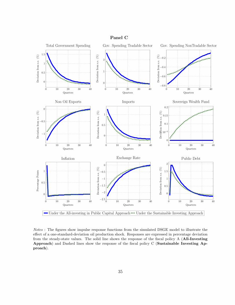
Panel C
0 10 20 30 40
0
0.5
1
1.5
Quarters
Dev
iati
onfr
oms.
s.(%
)
Total Government Spending
0 10 20 30 40
0
1
2
Quarters
Dev
iati
onfr
oms.
s.(%
)
Gov. Spending Tradable Sector
0 10 20 30 40−0.8
−0.6
−0.4
−0.2
Quarters
Dev
iati
onfr
oms.
s.(%
)
Gov. Spending NonTradable Sector
0 10 20 30 40
−1
−0.5
0
Quarters
Dev
iati
onfr
oms.
s.(%
)
Non Oil Exports
0 10 20 30 40
0
0.5
1
Quarters
Dev
iati
onfr
oms.
s.(%
)
Imports
0 10 20 30 40
0
5 · 10−2
0.1
0.15
0.2
Quarters
Dev
iati
onfr
oms.
s.(%
)
Sovereign Wealth Fund
0 10 20 30 40
0
0.5
1
Quarters
Per
centa
geP
oints
Inflation
0 10 20 30 40−2.5
−2
−1.5
−1
−0.5
0
Quarters
Dev
iati
onfr
oms.
s.(%
)
Exchange Rate
0 10 20 30 40
0
0.5
1
1.5
2
Quarters
Dev
iati
onfr
oms.
s.(%
)Public Debt
Under the All-investing in Public Capital Approach Under the Sustainable Investing Approach
Notes : The figures show impulse response functions from the simulated DSGE model toillustrate the effect of a one-standard-deviation oil production shock. Responses are
expressed in percentage deviation from the steady-state values. The solid line shows theresponse of the fiscal policy A (All-Investing Approach) and Dashed lines show the
response of the fiscal policy C (Sustainable Investing Approach).
57
Notes : The figures show impulse response functions from the simulated DSGE model to illustrate theeffect of a one-standard-deviation oil production shock. Responses are expressed in percentage deviationfrom the steady-state values. The solid line shows the response of the fiscal policy A (All-InvestingApproach) and Dashed lines show the response of the fiscal policy C (Sustainable Investing Ap-proach).
35
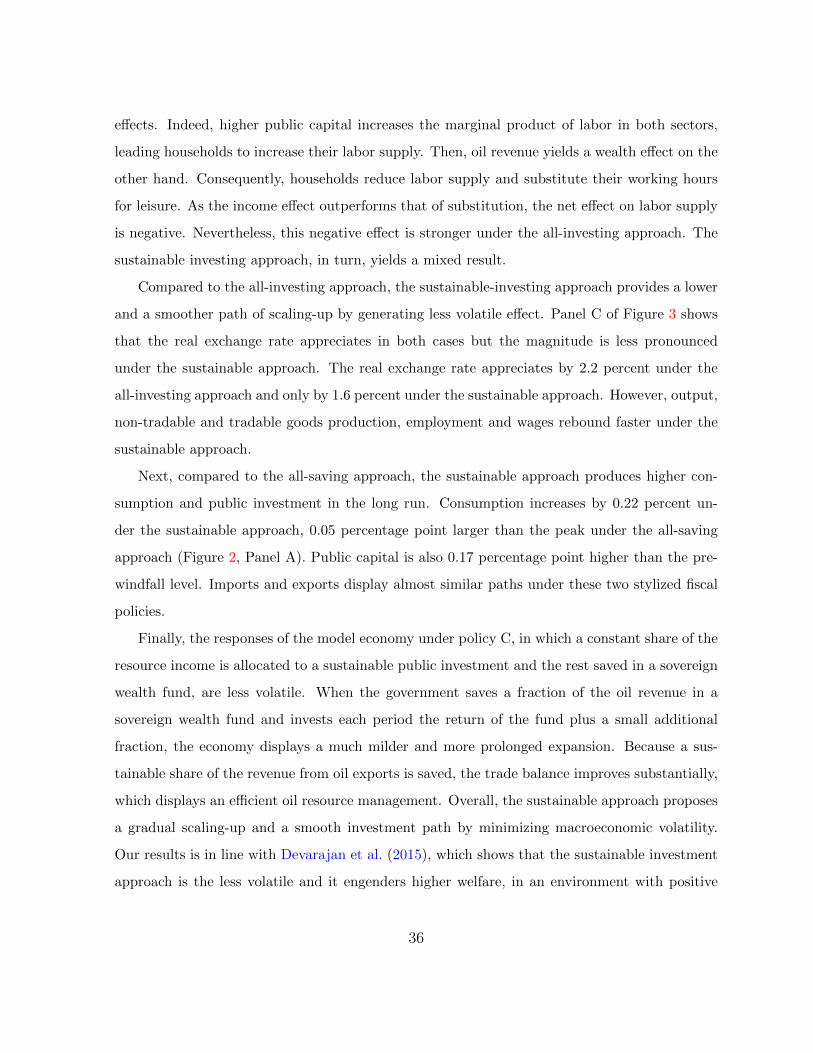
effects. Indeed, higher public capital increases the marginal product of labor in both sectors,
leading households to increase their labor supply. Then, oil revenue yields a wealth effect on the
other hand. Consequently, households reduce labor supply and substitute their working hours
for leisure. As the income effect outperforms that of substitution, the net effect on labor supply
is negative. Nevertheless, this negative effect is stronger under the all-investing approach. The
sustainable investing approach, in turn, yields a mixed result.
Compared to the all-investing approach, the sustainable-investing approach provides a lower
and a smoother path of scaling-up by generating less volatile effect. Panel C of Figure 3 shows
that the real exchange rate appreciates in both cases but the magnitude is less pronounced
under the sustainable approach. The real exchange rate appreciates by 2.2 percent under the
all-investing approach and only by 1.6 percent under the sustainable approach. However, output,
non-tradable and tradable goods production, employment and wages rebound faster under the
sustainable approach.
Next, compared to the all-saving approach, the sustainable approach produces higher con-
sumption and public investment in the long run. Consumption increases by 0.22 percent un-
der the sustainable approach, 0.05 percentage point larger than the peak under the all-saving
approach (Figure 2, Panel A). Public capital is also 0.17 percentage point higher than the pre-
windfall level. Imports and exports display almost similar paths under these two stylized fiscal
policies.
Finally, the responses of the model economy under policy C, in which a constant share of the
resource income is allocated to a sustainable public investment and the rest saved in a sovereign
wealth fund, are less volatile. When the government saves a fraction of the oil revenue in a
sovereign wealth fund and invests each period the return of the fund plus a small additional
fraction, the economy displays a much milder and more prolonged expansion. Because a sus-
tainable share of the revenue from oil exports is saved, the trade balance improves substantially,
which displays an efficient oil resource management. Overall, the sustainable approach proposes
a gradual scaling-up and a smooth investment path by minimizing macroeconomic volatility.
Our results is in line with Devarajan et al. (2015), which shows that the sustainable investment
approach is the less volatile and it engenders higher welfare, in an environment with positive
36
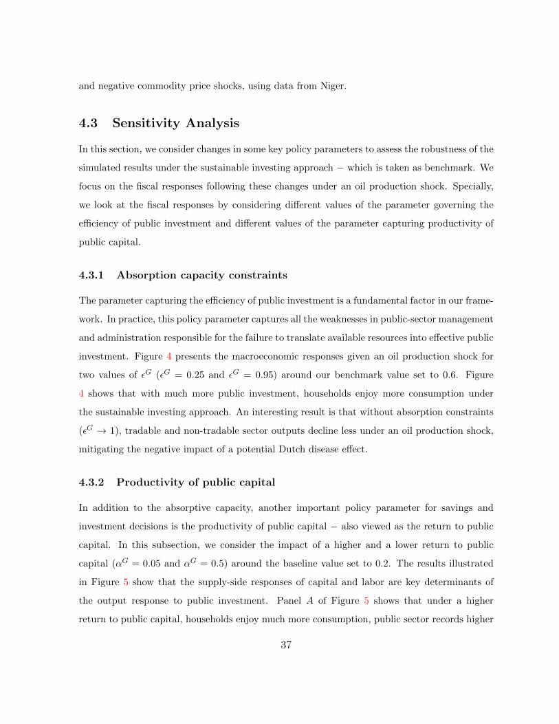
and negative commodity price shocks, using data from Niger.
4.3 Sensitivity Analysis
In this section, we consider changes in some key policy parameters to assess the robustness of the
simulated results under the sustainable investing approach − which is taken as benchmark. We
focus on the fiscal responses following these changes under an oil production shock. Specially,
we look at the fiscal responses by considering different values of the parameter governing the
efficiency of public investment and different values of the parameter capturing productivity of
public capital.
4.3.1 Absorption capacity constraints
The parameter capturing the efficiency of public investment is a fundamental factor in our frame-
work. In practice, this policy parameter captures all the weaknesses in public-sector management
and administration responsible for the failure to translate available resources into effective public
investment. Figure 4 presents the macroeconomic responses given an oil production shock for
two values of εG (εG = 0.25 and εG = 0.95) around our benchmark value set to 0.6. Figure
4 shows that with much more public investment, households enjoy more consumption under
the sustainable investing approach. An interesting result is that without absorption constraints
(εG → 1), tradable and non-tradable sector outputs decline less under an oil production shock,
mitigating the negative impact of a potential Dutch disease effect.
4.3.2 Productivity of public capital
In addition to the absorptive capacity, another important policy parameter for savings and
investment decisions is the productivity of public capital − also viewed as the return to public
capital. In this subsection, we consider the impact of a higher and a lower return to public
capital (αG = 0.05 and αG = 0.5) around the baseline value set to 0.2. The results illustrated
in Figure 5 show that the supply-side responses of capital and labor are key determinants of
the output response to public investment. Panel A of Figure 5 shows that under a higher
return to public capital, households enjoy much more consumption, public sector records higher
37
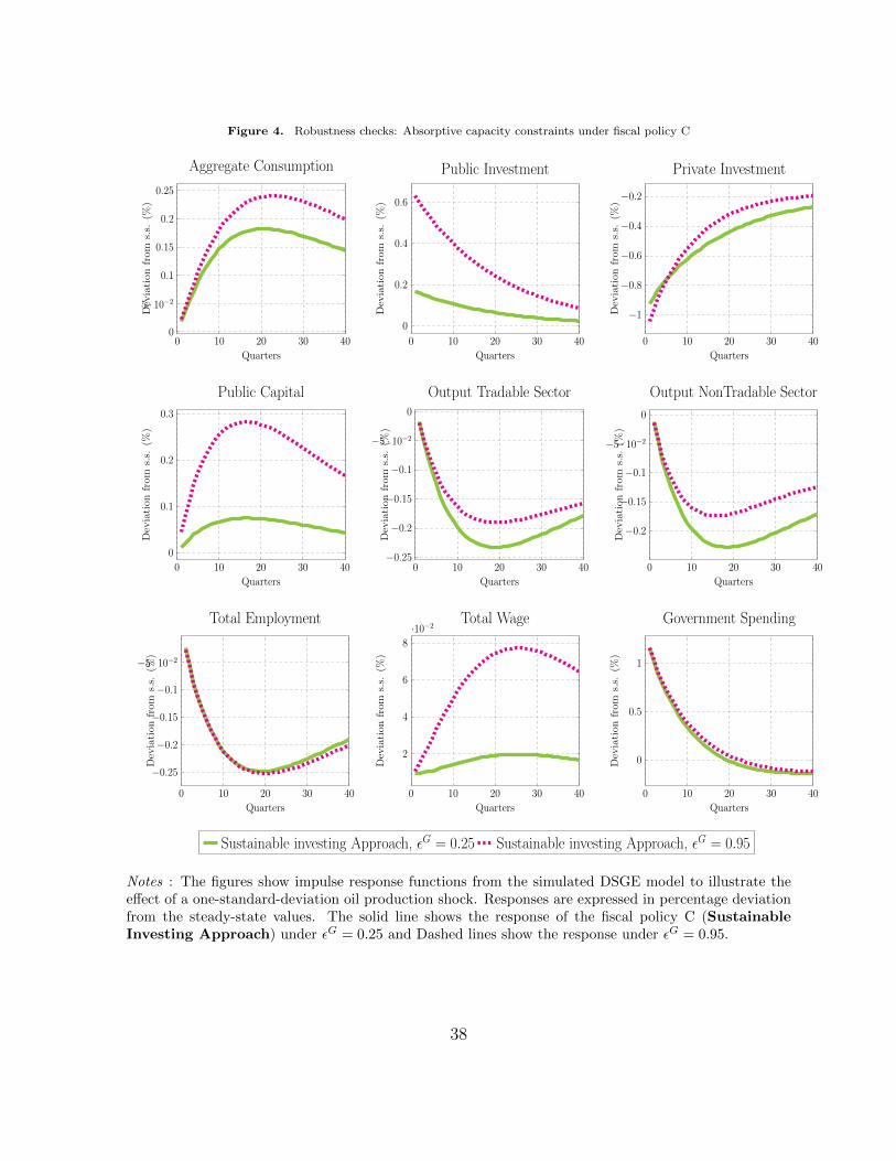
Figure 4. Robustness checks: Absorptive capacity constraints under fiscal policy CTable 6: Robustness checks: Absorptive capacity constraints under fiscal policy C
0 10 20 30 400
5 · 10−2
0.1
0.15
0.2
0.25
Quarters
Dev
iati
on
from
s.s.
(%)
Aggregate Consumption
0 10 20 30 40
0
0.2
0.4
0.6
Quarters
Dev
iati
on
from
s.s.
(%)
Public Investment
0 10 20 30 40
−1
−0.8
−0.6
−0.4
−0.2
Quarters
Dev
iati
on
from
s.s.
(%)
Private Investment
0 10 20 30 40
0
0.1
0.2
0.3
Quarters
Dev
iati
on
from
s.s.
(%)
Public Capital
0 10 20 30 40−0.25
−0.2
−0.15
−0.1
−5 · 10−2
0
Quarters
Dev
iati
on
from
s.s.
(%)
Output Tradable Sector
0 10 20 30 40
−0.2
−0.15
−0.1
−5 · 10−2
0
Quarters
Dev
iati
on
from
s.s.
(%)
Output NonTradable Sector
0 10 20 30 40
−0.25
−0.2
−0.15
−0.1
−5 · 10−2
Quarters
Dev
iati
on
from
s.s.
(%)
Total Employment
0 10 20 30 40
2
4
6
8
·10−2
Quarters
Dev
iati
on
from
s.s.
(%)
Total Wage
0 10 20 30 40
0
0.5
1
Quarters
Dev
iati
on
from
s.s.
(%)
Government Spending
Sustainable investing Approach, εG = 0.25 Sustainable investing Approach, εG = 0.95
Notes : The figures show impulse response functions from the simulated DSGE model toillustrate the effect of a one-standard-deviation oil production shock. Responses are
expressed in percentage deviation from the steady-state values. The solid line shows theresponse of the fiscal policy C (Sustainable Investing Approach) under εG = 0.25
and Dashed lines show the response under εG = 0.95.
58
Notes : The figures show impulse response functions from the simulated DSGE model to illustrate theeffect of a one-standard-deviation oil production shock. Responses are expressed in percentage deviationfrom the steady-state values. The solid line shows the response of the fiscal policy C (SustainableInvesting Approach) under εG = 0.25 and Dashed lines show the response under εG = 0.95.
38
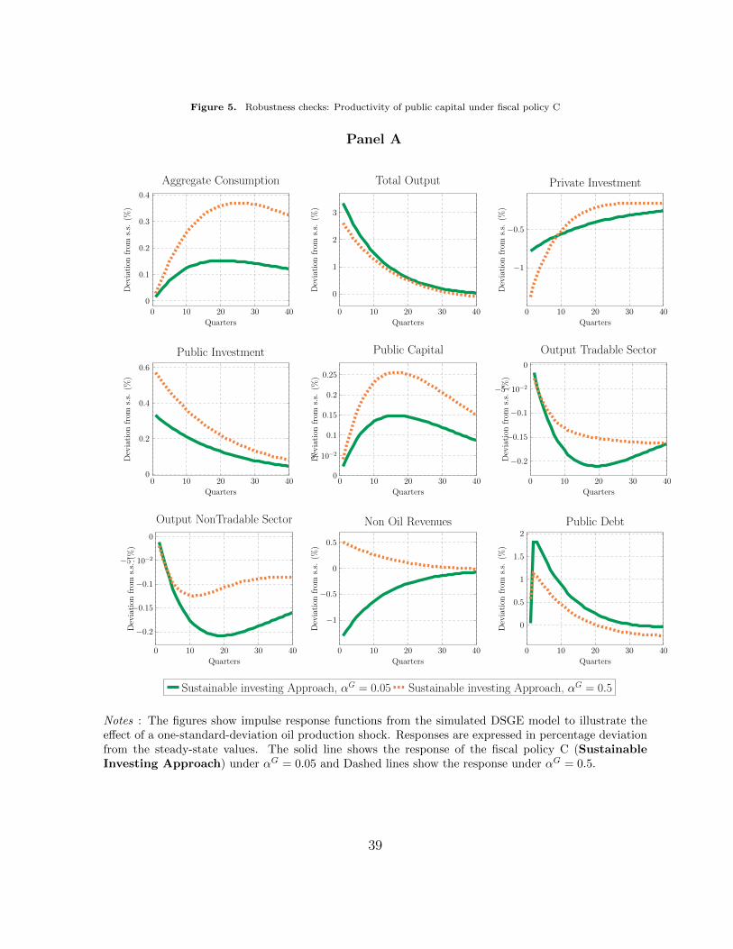
Figure 5. Robustness checks: Productivity of public capital under fiscal policy CTable 7: Robustness checks: Productivity of public capital under fiscal policy C
Panel A
0 10 20 30 40
0
0.1
0.2
0.3
0.4
Quarters
Dev
iati
onfr
oms.
s.(%
)
Aggregate Consumption
0 10 20 30 40
0
1
2
3
QuartersD
evia
tion
from
s.s.
(%)
Total Output
0 10 20 30 40
−1
−0.5
Quarters
Dev
iati
onfr
oms.
s.(%
)
Private Investment
0 10 20 30 400
0.2
0.4
0.6
Quarters
Dev
iati
onfr
oms.
s.(%
)
Public Investment
0 10 20 30 400
5 · 10−2
0.1
0.15
0.2
0.25
Quarters
Dev
iati
onfr
oms.
s.(%
)
Public Capital
0 10 20 30 40
−0.2
−0.15
−0.1
−5 · 10−2
0
Quarters
Dev
iati
onfr
oms.
s.(%
)
Output Tradable Sector
0 10 20 30 40
−0.2
−0.15
−0.1
−5 · 10−2
0
Quarters
Dev
iati
onfr
oms.
s.(%
)
Output NonTradable Sector
0 10 20 30 40
−1
−0.5
0
0.5
Quarters
Dev
iati
onfr
oms.
s.(%
)
Non Oil Revenues
0 10 20 30 40
0
0.5
1
1.5
2
Quarters
Dev
iati
onfr
oms.
s.(%
)
Public Debt
Sustainable investing Approach, αG = 0.05 Sustainable investing Approach, αG = 0.5
Notes : The figures show impulse response functions from the simulated DSGE model toillustrate the effect of a one-standard-deviation oil production shock. Responses are
expressed in percentage deviation from the steady-state values. The solid line shows theresponse of the fiscal policy C (Sustainable Investing Approach) under αG = 0.05
and Dashed lines show the response under αG = 0.5.
59
Notes : The figures show impulse response functions from the simulated DSGE model to illustrate theeffect of a one-standard-deviation oil production shock. Responses are expressed in percentage deviationfrom the steady-state values. The solid line shows the response of the fiscal policy C (SustainableInvesting Approach) under αG = 0.05 and Dashed lines show the response under αG = 0.5.
39
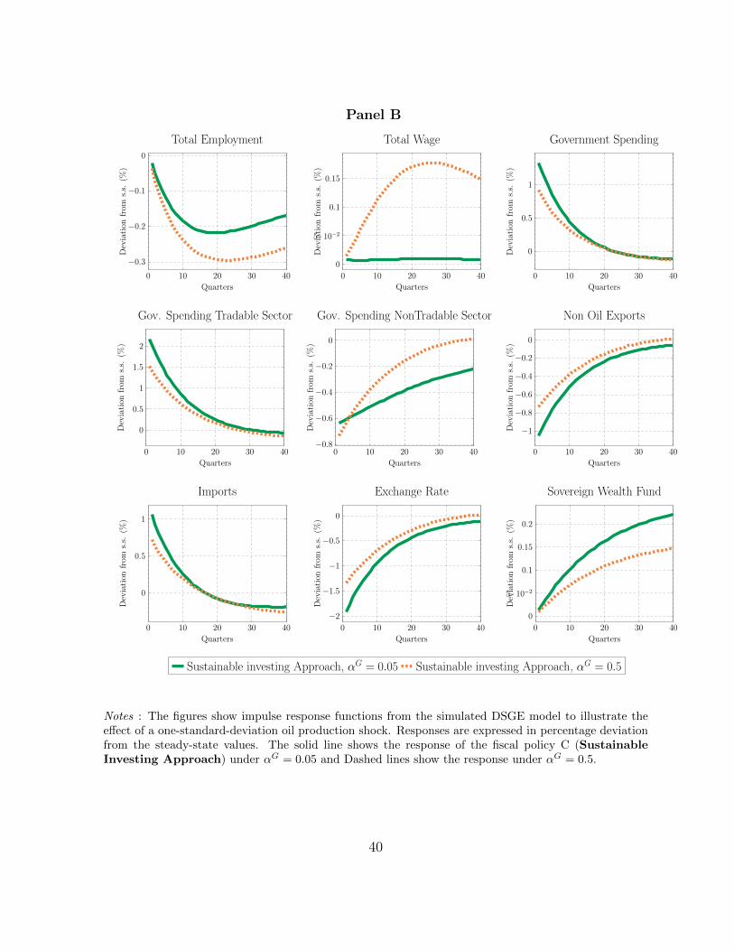
Panel B
0 10 20 30 40
−0.3
−0.2
−0.1
0
Quarters
Dev
iati
onfr
oms.
s.(%
)
Total Employment
0 10 20 30 40
0
5 · 10−2
0.1
0.15
Quarters
Dev
iati
onfr
oms.
s.(%
)
Total Wage
0 10 20 30 40
0
0.5
1
Quarters
Dev
iati
onfr
oms.
s.(%
)
Government Spending
0 10 20 30 40
0
0.5
1
1.5
2
Quarters
Dev
iati
onfr
oms.
s.(%
)
Gov. Spending Tradable Sector
0 10 20 30 40−0.8
−0.6
−0.4
−0.2
0
Quarters
Dev
iati
onfr
oms.
s.(%
)Gov. Spending NonTradable Sector
0 10 20 30 40
−1
−0.8
−0.6
−0.4
−0.2
0
Quarters
Dev
iati
onfr
oms.
s.(%
)
Non Oil Exports
0 10 20 30 40
0
0.5
1
Quarters
Dev
iati
onfr
oms.
s.(%
)
Imports
0 10 20 30 40
−2
−1.5
−1
−0.5
0
Quarters
Dev
iati
onfr
oms.
s.(%
)
Exchange Rate
0 10 20 30 40
0
5 · 10−2
0.1
0.15
0.2
Quarters
Dev
iati
onfr
oms.
s.(%
)
Sovereign Wealth Fund
Sustainable investing Approach, αG = 0.05 Sustainable investing Approach, αG = 0.5
Notes : The figures show impulse response functions from the simulated DSGE model toillustrate the effect of a one-standard-deviation oil production shock. Responses are
expressed in percentage deviation from the steady-state values. The solid line shows theresponse of the fiscal policy C (Sustainable Investing Approach) under αG = 0.05
and Dashed lines show the response under αG = 0.5.
60
Notes : The figures show impulse response functions from the simulated DSGE model to illustrate theeffect of a one-standard-deviation oil production shock. Responses are expressed in percentage deviationfrom the steady-state values. The solid line shows the response of the fiscal policy C (SustainableInvesting Approach) under αG = 0.05 and Dashed lines show the response under αG = 0.5.
40

public investment and output in tradable and non-tradable sectors declines less compared to the
scenario where public is almost unproductive αG = 0.05. Panel B of Figure 5 shows that when
investment projects are almost unproductive (αG = 0.05), households are better off saving in a
sovereign wealth fund and consuming the interest income. Although investing natural resource
revenues in public infrastructures might be viewed as an attractive fiscal policy to accelerate
economic development in public capital-scarce economies, a better fiscal management is to save
the resource income in a sovereign fund for future generation when public capital is almost
unproductive.
4.4 Optimal allocation of natural resource revenues
The previous analysis has focused on the benchmark model in which the parameter governing
the share of resource windfalls allocated to public investment is exogenously set to 0.5. Under
this fiscal rule, half of the resource income is saved in a sovereign wealth fund and the remaining
half combined to the interest rate payments received are used to finance public infrastructure.
However, a key fiscal policy issue is the following: given the poor return to public capital and
significant absorptive capacity constraints in the economy, what should be the optimal allocation
of resource revenues between public infrastructure financing and saving in a sovereign wealth
fund? In other words what is the value of φoil that optimizes the objective function of the
policy maker? The answer to this question requires that the policy maker’s objective function
be defined. To assess the optimal allocation of the resource income to public infrastructures
under the sustainable investing approach and come out with a well defined loss function, we
focus on the volatility of four important macroeconomic variables: private consumption (σC),
total employment (σL), non-oil fiscal balance (σFBNO) and real exchange rate (σs).
Conceptually, we propose a criterion consisting to determine the value of φoil that minimizes
a social loss function. Our loss function closely resembles that used by Agenor (2014); it is
indeed defined as a weighted geometric average of a welfare measure and a fiscal/macroeconomic
stability measure. The welfare measure is either captured by the volatility of consumption or
by an equally weighted geometric average of the volatility of consumption and that of total
employment. In our model, households as risk averse agents dislike volatile private consumption
41
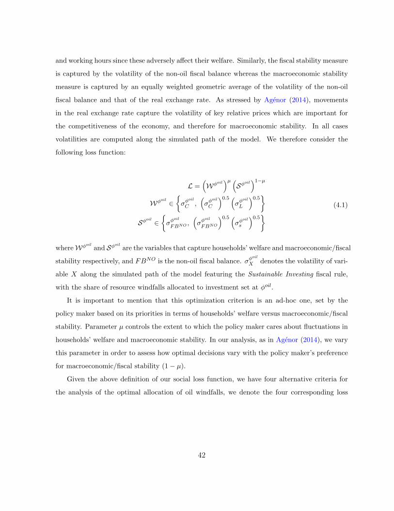
and working hours since these adversely affect their welfare. Similarly, the fiscal stability measure
is captured by the volatility of the non-oil fiscal balance whereas the macroeconomic stability
measure is captured by an equally weighted geometric average of the volatility of the non-oil
fiscal balance and that of the real exchange rate. As stressed by Agenor (2014), movements
in the real exchange rate capture the volatility of key relative prices which are important for
the competitiveness of the economy, and therefore for macroeconomic stability. In all cases
volatilities are computed along the simulated path of the model. We therefore consider the
following loss function:
L =(Wφoil
)µ (Sφoil
)1−µ
Wφoil ∈σφ
oil
C ,(σφ
oil
C
)0.5 (σφ
oil
L
)0.5
Sφoil ∈σφ
oil
FBNO,(σφ
oil
FBNO
)0.5 (σφ
oil
s
)0.5 (4.1)
whereWφoil and Sφoil are the variables that capture households’ welfare and macroeconomic/fiscal
stability respectively, and FBNO is the non-oil fiscal balance. σφoil
X denotes the volatility of vari-
able X along the simulated path of the model featuring the Sustainable Investing fiscal rule,
with the share of resource windfalls allocated to investment set at φoil.
It is important to mention that this optimization criterion is an ad-hoc one, set by the
policy maker based on its priorities in terms of households’ welfare versus macroeconomic/fiscal
stability. Parameter µ controls the extent to which the policy maker cares about fluctuations in
households’ welfare and macroeconomic stability. In our analysis, as in Agenor (2014), we vary
this parameter in order to assess how optimal decisions vary with the policy maker’s preference
for macroeconomic/fiscal stability (1− µ).
Given the above definition of our social loss function, we have four alternative criteria for
the analysis of the optimal allocation of oil windfalls, we denote the four corresponding loss
42
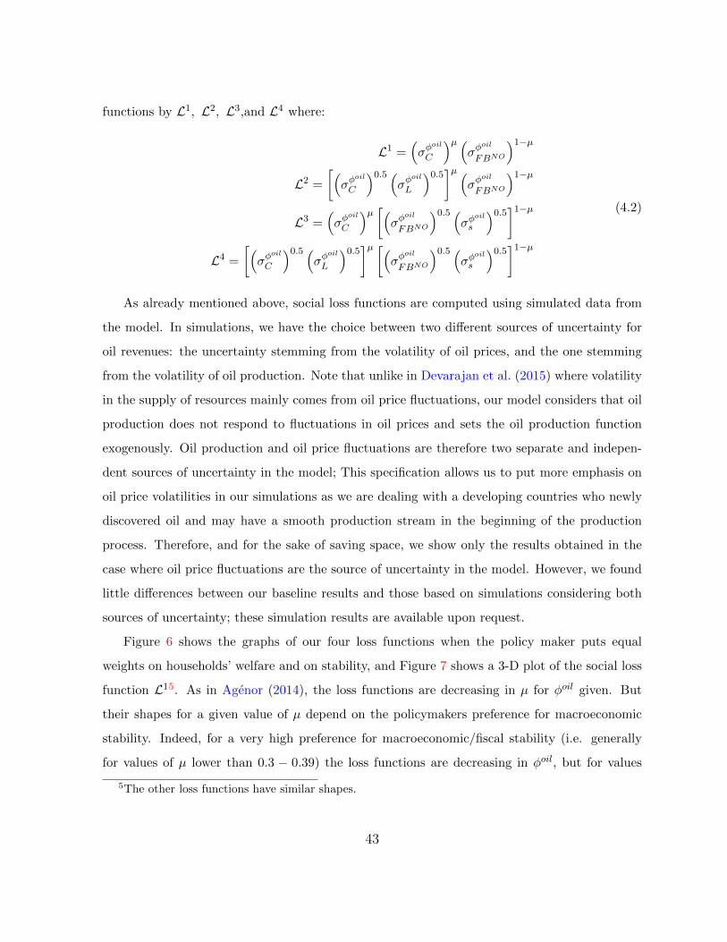
functions by L1, L2, L3,and L4 where:
L1 =(σφ
oil
C
)µ (σφ
oil
FBNO
)1−µ
L2 =
[(σφ
oil
C
)0.5 (σφ
oil
L
)0.5]µ (
σφoil
FBNO
)1−µ
L3 =(σφ
oil
C
)µ [(σφ
oil
FBNO
)0.5 (σφ
oil
s
)0.5]1−µ
L4 =
[(σφ
oil
C
)0.5 (σφ
oil
L
)0.5]µ [(
σφoil
FBNO
)0.5 (σφ
oil
s
)0.5]1−µ
(4.2)
As already mentioned above, social loss functions are computed using simulated data from
the model. In simulations, we have the choice between two different sources of uncertainty for
oil revenues: the uncertainty stemming from the volatility of oil prices, and the one stemming
from the volatility of oil production. Note that unlike in Devarajan et al. (2015) where volatility
in the supply of resources mainly comes from oil price fluctuations, our model considers that oil
production does not respond to fluctuations in oil prices and sets the oil production function
exogenously. Oil production and oil price fluctuations are therefore two separate and indepen-
dent sources of uncertainty in the model; This specification allows us to put more emphasis on
oil price volatilities in our simulations as we are dealing with a developing countries who newly
discovered oil and may have a smooth production stream in the beginning of the production
process. Therefore, and for the sake of saving space, we show only the results obtained in the
case where oil price fluctuations are the source of uncertainty in the model. However, we found
little differences between our baseline results and those based on simulations considering both
sources of uncertainty; these simulation results are available upon request.
Figure 6 shows the graphs of our four loss functions when the policy maker puts equal
weights on households’ welfare and on stability, and Figure 7 shows a 3-D plot of the social loss
function L15. As in Agenor (2014), the loss functions are decreasing in µ for φoil given. But
their shapes for a given value of µ depend on the policymakers preference for macroeconomic
stability. Indeed, for a very high preference for macroeconomic/fiscal stability (i.e. generally
for values of µ lower than 0.3 − 0.39) the loss functions are decreasing in φoil, but for values
5The other loss functions have similar shapes.
43
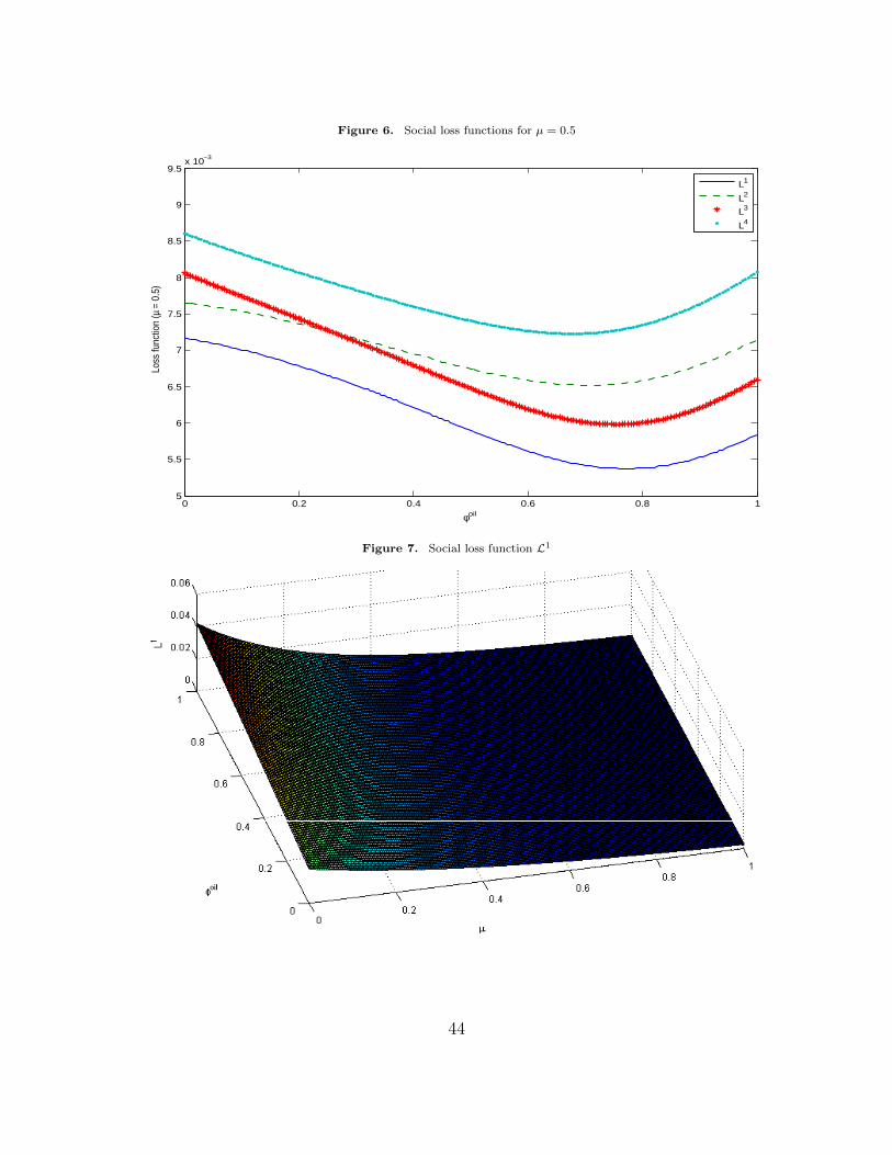
Figure 6. Social loss functions for µ = 0.5
0 0.2 0.4 0.6 0.8 15
5.5
6
6.5
7
7.5
8
8.5
9
9.5x 10
−3Lo
ss fu
nctio
n (µ
= 0
.5)
φoil
L1
L2
L3
L4
Figure 7. Social loss function L1
44
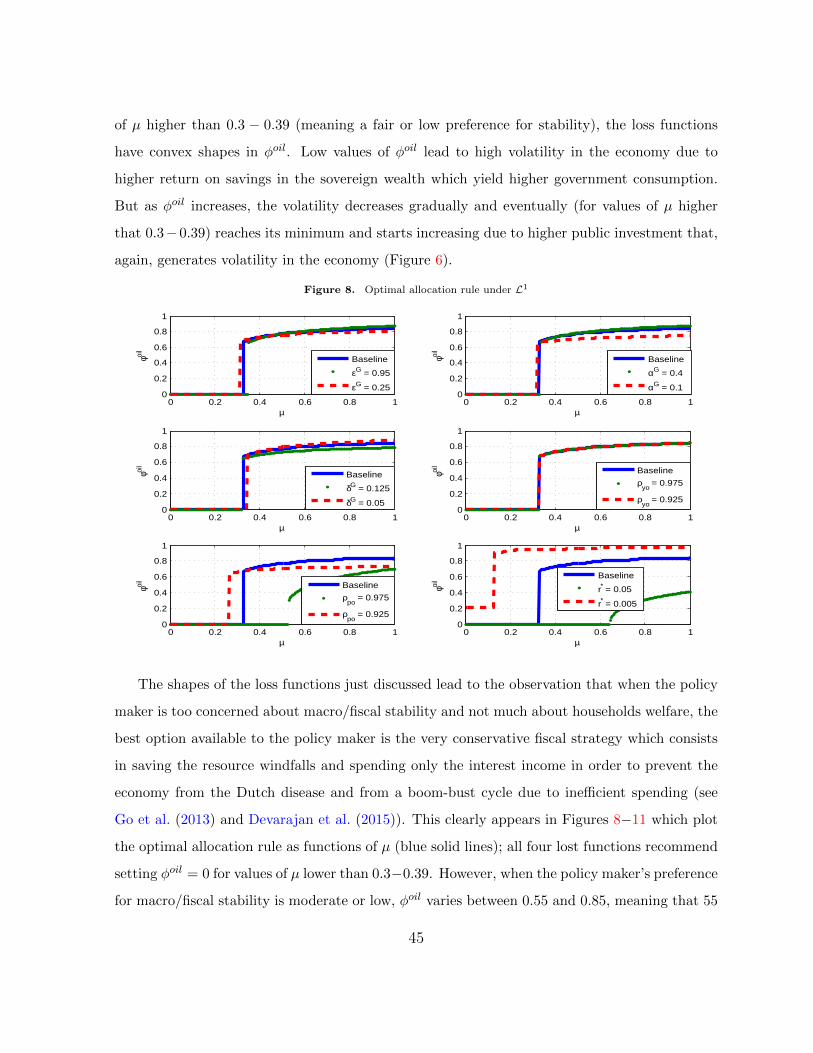
of µ higher than 0.3 − 0.39 (meaning a fair or low preference for stability), the loss functions
have convex shapes in φoil. Low values of φoil lead to high volatility in the economy due to
higher return on savings in the sovereign wealth which yield higher government consumption.
But as φoil increases, the volatility decreases gradually and eventually (for values of µ higher
that 0.3−0.39) reaches its minimum and starts increasing due to higher public investment that,
again, generates volatility in the economy (Figure 6).
Figure 8. Optimal allocation rule under L1
0 0.2 0.4 0.6 0.8 10
0.2
0.4
0.6
0.8
1
φoil
µ
Baseline
εG = 0.95
εG = 0.25
0 0.2 0.4 0.6 0.8 10
0.2
0.4
0.6
0.8
1
φoil
µ
Baseline
αG = 0.4
αG = 0.1
0 0.2 0.4 0.6 0.8 10
0.2
0.4
0.6
0.8
1
φoil
µ
Baseline
δG = 0.125
δG = 0.05
0 0.2 0.4 0.6 0.8 10
0.2
0.4
0.6
0.8
1φoi
l
µ
Baseline
ρyo
= 0.975
ρyo
= 0.925
0 0.2 0.4 0.6 0.8 10
0.2
0.4
0.6
0.8
1
φoil
µ
Baseline
ρpo
= 0.975
ρpo
= 0.925
0 0.2 0.4 0.6 0.8 10
0.2
0.4
0.6
0.8
1
φoil
µ
Baseline
r* = 0.05
r* = 0.005
The shapes of the loss functions just discussed lead to the observation that when the policy
maker is too concerned about macro/fiscal stability and not much about households welfare, the
best option available to the policy maker is the very conservative fiscal strategy which consists
in saving the resource windfalls and spending only the interest income in order to prevent the
economy from the Dutch disease and from a boom-bust cycle due to inefficient spending (see
Go et al. (2013) and Devarajan et al. (2015)). This clearly appears in Figures 8−11 which plot
the optimal allocation rule as functions of µ (blue solid lines); all four lost functions recommend
setting φoil = 0 for values of µ lower than 0.3−0.39. However, when the policy maker’s preference
for macro/fiscal stability is moderate or low, φoil varies between 0.55 and 0.85, meaning that 55
45
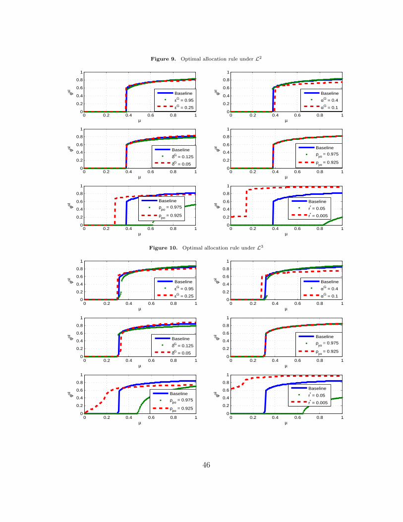
Figure 9. Optimal allocation rule under L2
0 0.2 0.4 0.6 0.8 10
0.2
0.4
0.6
0.8
1φoi
l
µ
Baseline
εG = 0.95
εG = 0.25
0 0.2 0.4 0.6 0.8 10
0.2
0.4
0.6
0.8
1
φoil
µ
Baseline
αG = 0.4
αG = 0.1
0 0.2 0.4 0.6 0.8 10
0.2
0.4
0.6
0.8
1
φoil
µ
Baseline
δG = 0.125
δG = 0.05
0 0.2 0.4 0.6 0.8 10
0.2
0.4
0.6
0.8
1
φoil
µ
Baseline
ρyo
= 0.975
ρyo
= 0.925
0 0.2 0.4 0.6 0.8 10
0.2
0.4
0.6
0.8
1
φoil
µ
Baseline
ρpo
= 0.975
ρpo
= 0.925
0 0.2 0.4 0.6 0.8 10
0.2
0.4
0.6
0.8
1
φoil
µ
Baseline
r* = 0.05
r* = 0.005
Figure 10. Optimal allocation rule under L3
0 0.2 0.4 0.6 0.8 10
0.2
0.4
0.6
0.8
1
φoil
µ
Baseline
εG = 0.95
εG = 0.25
0 0.2 0.4 0.6 0.8 10
0.2
0.4
0.6
0.8
1
φoil
µ
Baseline
αG = 0.4
αG = 0.1
0 0.2 0.4 0.6 0.8 10
0.2
0.4
0.6
0.8
1
φoil
µ
Baseline
δG = 0.125
δG = 0.05
0 0.2 0.4 0.6 0.8 10
0.2
0.4
0.6
0.8
1
φoil
µ
Baseline
ρyo
= 0.975
ρyo
= 0.925
0 0.2 0.4 0.6 0.8 10
0.2
0.4
0.6
0.8
1
φoil
µ
Baseline
ρpo
= 0.975
ρpo
= 0.925
0 0.2 0.4 0.6 0.8 10
0.2
0.4
0.6
0.8
1
φoil
µ
Baseline
r* = 0.05
r* = 0.005
46

Figure 11. Optimal allocation rule under L4
0 0.2 0.4 0.6 0.8 10
0.2
0.4
0.6
0.8
1φoi
l
µ
Baseline
εG = 0.95
εG = 0.25
0 0.2 0.4 0.6 0.8 10
0.2
0.4
0.6
0.8
1
φoil
µ
Baseline
αG = 0.4
αG = 0.1
0 0.2 0.4 0.6 0.8 10
0.2
0.4
0.6
0.8
1
φoil
µ
Baseline
δG = 0.125
δG = 0.05
0 0.2 0.4 0.6 0.8 10
0.2
0.4
0.6
0.8
1
φoil
µ
Baseline
ρyo
= 0.975
ρyo
= 0.925
0 0.2 0.4 0.6 0.8 10
0.2
0.4
0.6
0.8
1
φoil
µ
Baseline
ρpo
= 0.975
ρpo
= 0.925
0 0.2 0.4 0.6 0.8 10
0.2
0.4
0.6
0.8
1
φoil
µ
Baseline
r* = 0.05
r* = 0.005
to 85 percent of oil windfalls should be used for public investment. This share increases with
µ and does not depend much on the loss function used. Although this range include values
that are very high compared to values generally found in the literature, we think that they are
reasonable for a country that newly discovered oil, and for which the oil production process is
not as volatile and uncertain as experienced oil producers. Being a new oil producer reduces
a the volatility stemming from oil production in the beginning of the extraction process and
therefore reduces the need for savings.
A welfare comparison of alternative fiscal rules in an economy enduring volatile and uncertain
resource price leads Devarajan et al. (2015) to recommend a combination of savings and public
investment as the best way to cope with volatile oil revenues due to unpredictable shocks. Their
analysis is a special case of ours (when µ = 1) but we go beyond their recommendation by
stressing that if households’ welfare is the only concern of the policy maker, then 80 percent to
85 percent of resource windfalls should be allocated to public investment instead of assuming
50 percent for saving and 50 percent investment as a sustainable approach. Public investment
improves households’ welfare mainly through the positive effect that public infrastructure has
47
on private capital and labor productivity.
Robustness checks show that our findings do not on depend key parameters of the model
apart from those which directly affect resource revenues such as the persistence of oil price
shocks (ρpo) and the interest rate paid on sovereign funds (r∗). Indeed, the red dashed lines
and the green dotted lines in Figures 8−11 show the optimal allocation rule for two alternative
values of each of the parameters indicated. The middle right panels of these figures show that
the rules, under the alternative parameterizations of the persistence of the oil production shock,
are similar to the baseline as oil production is exogenously determined in our model. The top
panels and the middle left panel show that the efficiency of public investment, εG, the output
elasticity of public capital, αG, as well as the depreciation rate of public capital, δG, only play a
minor role in determining the optimal allocation of resource windfalls. However, the interest rate
paid on sovereign funds (bottom right panels) is an important driver of the resource allocation.
Our analysis suggests on the one hand that when funds saved abroad do not generate enough
income because of very low interest rates, then the policy maker should invest 20 percent of the
windfall if he is extremely worried about stability, but otherwise almost all (90 percent to 98
percent) the windfall should be used for public investment. On the other hand, if the interest
paid on sovereign funds are very high, the best strategy is to invest only if households’ welfare is
of very high concern; in this case, only up to 40 percent of the windfall should be invested, and
the remaining share saved. Additional robustness checks show that more windfalls should be
saved in the sovereign wealth fund when oil price shocks are very persistent (green dotted lines
in bottom left panels of Figures 8−11), or invested when oil price shocks are less persistent.
5 Concluding Remarks
In this paper we studied different fiscal policy approaches of investing a resource windfall through
a small open economy DSGE model applied to Uganda. Specifically, we study macroeconomic
dynamics following three stylized fiscal policy approaches: the all-investing approach, the all-
saving approach and the sustainable-investing approach in which a constant share of the resource
income is allocated to public investment. The model accounts for several important features that
48
are common in the New Keynesian model literature applied to developing countries, including
Dutch disease effects, investment inefficiencies and weak tax systems. The model is parameter-
ized following various empirical works and data from Uganda, and is used to simulate the effects
of a one standard deviation oil production shock, interpreted as a boom in the energy sector.
Our results show that: (i) a better fiscal management is to save the resource income in a
sovereign wealth fund for future generation when public capital is almost unproductive; (ii) a
gradual scaling-up of public investment (The Sustainable-Investing Approach) yields the best
outcomes as it minimizes macroeconomic volatility; e.g. the real exchange rate appreciation is
30 percent lower than in the all-investing approach, which might be viewed as an attractive fiscal
policy to accelerate economic development in public capital-scarce economies; the trade balance
improves substantially and impulse response functions suggest that output, non-tradable and
tradable goods production, employment and wages rebound faster.
We also define criteria to determine the optimal value of the oil share to invest in public
infrastructures by minimizing a social loss function; we use four loss functions that include a
households’ welfare indicator and a macroeconomic/fiscal stabilization indicator. We find that
the loss functions have convex shapes with optimal values of φoil varying between 0.55 and
0.85, depending on the policy maker’s preference for macroeconomic stability. Furthermore,
our results show that the optimal share of oil revenues to be used for public investment is very
robust to the various parameter calibrations; only parameters that directly affect these revenues
(such as interest rates on savings and the persistence of oil price shocks) play an important
role. In comparison with the recent literature, our optimal share to invest domestically in public
infrastructures is slightly higher than those estimated in Agenor (2014), which ranges from 30
percent to 60 percent using oil price shocks.
A number of extensions could usefully be considered. First, the paper assumes an exogenous
oil sector, and the analysis can be extended to explore labor movements between non-oil and
oil sectors. In practice, oil sectors in developing countries use domestic labor and Dutch disease
effects can be optimally analyzed using an endogenous oil production sector. Second, the paper
does not consider the effect of foreign direct investments (FDI). Indeed, it’s well-known that
in low-income countries, FDI account substantially and may affect macroeconomic dynamics.
49
Third, the model focuses on some standard government rules and our sustainable approach can
be improved to take into account a sovereign wealth fund that can serve as a stabilization buffer,
enabling households and government to smooth consumption and public investment paths over
negative economic shocks. Finally, our analysis suggests that a high proportion of oil revenues
should be invested, but does not specify which type of investment should be prioritized. The
analysis could be deepened so as to determine how much of the resources should be used to
increase soft/hard infrastructure.
References
Agenor, P. R. (2014). Optimal fiscal management of commodity price shocks. Centre for Growth
and Business Cycle Research Discussion Paper Series, 197. Economics, The Univeristy of
Manchester.
Aikman, D. and Paustian, M. (2006). Bank capital, asset prices and monetary policy. Working
paper, Bank of England 2006-305.
Ambler, S., Dib, A., and Rebei, N. (2004). Optimal taylor rules in estimated model of small
open economy. Working paper, Bank of Canada 2004-36.
Angenor, P. R. and Aizenman, J. (1999). Macroeconomic adjustment with segmented labor
markets. Journal of Development Economics, 58.
Arestoff, F. and Hurlin, C. (2006). Estimates of government net capital stocks for 26 developing
countries 1970-2002. World Bank Policy Research Working Paper 3858.
Backus, D., Kehoe, P., and Kydland, F. (1994). Dynamics of the trade balance and the terms
of trade: the j-curve? American Economic Review 84 (1), pages 84–103.
Backus, D., Kehoe, P., and Kydland, F. (1995). International business cycles: theory and
evidence. In: Cooley, T.F. (Ed.), Frontiers of Business Cycle Research. Princeton University
Press, Princeton, pages 331–356.
50
Barnett, S. and Ossowski, R. (2003). Operational aspects of fiscal policy in oil-producing coun-
tries. in J. Davis, J. Ossowski, and A. Fedelino, eds., Fiscal Policy Formulation and Imple-
mentation in Oil-Producing Countries, (Washington, D.C.: International Monetary Fund.
Baunsgaard, T., Villafuerte, M., Poplawski-Ribeiro, M., and Richmond, C. (2012). Fiscal frame-
works for resource rich developing countries. Staff Discussion Note, International Monetary
Fund, page 12/04.
Baxter, M. (1995). International trade and business cycles. In: Grossmann, G.M., Rogoff, K.
(Eds.), Handbook of International Economics, pages 1801–1864.
Baxter, M. and King, R. (1993). Fiscal policy in general equilibrium. American Economic
Review, vol. 86, pages 1154–1174.
Berg, A., Portillo, R., Yang, S., and Zanna, L.-F. (2013). Public investment in resource-abundant
developing countries. IMF Economic Review, 61, pages 92–129.
Berms, R. and Irineu, C., F. (2011). The current account and precautionary savings for exporters
of exhaustible resources. Journal of International Economics, vol. 84, pages 48–64.
Cherif, R. and Fuad, H. (2012). Oil exporters’ dilemma: How much to save and how much to
invest. IMF Working Paper WP/12/4, International Monetary Fund.
Christensen, I. and Dib, A. (2008). The financial accelerator in an estimated new keynesian
model. Review of Economic Dynamics.
Christiano, L., Eichenbaum, M., and Evans, C. (2005). Nominal rigidities and the dynamic
effects of a shock to monetary policy. Journal of Political Economy.
Christiano, L., Motto, R., and Rostagno, M. (2010). Financial factors in economic fluctuations.
European Central Bank Working Paper, pages 555–576.
Christopher, A. and Bevan, D. (2006). Aid and the supply side: Public investment, export
performance, and dutch disease in low-income countries. World Bank Economic Review,
pages 261–90.
51
Collier, P., van der Ploeg, F., Spence, M., and Venables, A. (2010). Managing resource revenues
in developing economies. IMF Staff Papers, 51, pages 84–118.
Dagher, J., Gottschalk, J., and Portillo, R. (2012). The short-run impact of oil windfalls in
low-income countries: A dsge approach. Journal of African Economies, 21, pages 343–72.
Davis, J., Owssowski, J., Daniel, J., and Darnett, S. (2001). Stabilizing and saving funds
for non-renewable resources: Experience and fiscal policy implications. (Washington, D.C.:
International Monetary Fund). IMF Occasional Paper, no. 205.
Devarajan, S., Dissou, Y., Go, D., and Robinson, S. (2015). Budget rules and resource booms
and busts: A dynamic stochastic general equilibrium analysis. Policy Research Working Paper
Series 6984, The World Bank.
Economides, G., Park, H., and Philippopoulos, A. (2011). How should the government allo-
cate its tax revenues between productivity-enhancing and utility-enhancing public goods?
Macroeconomic Dynamics, 15, pages 336–64.
Gelb, A. and Grasmann, S. (2010). How should oil exporters spend their rents? Center for
Global Development, Working Paper No. 221.
Giovanni, M., Shu-Chun, S. Y., and Zanna, L.-F. (2014). Debt sustainability, public invest-
ment, and natural resources in developing countries: the dignar model. IMF Working Paper
WP/14/50.
Go, D., Robinson, S., Thierfelder, K., and Utz, R. (2013). Dutch disease and spending strategies
in a resource-rich low-income country – the case of niger. Policy Research Working Paper
Series 6691, The World Bank.
Goldberg, J. (2011). Kwacha gonna do? experimental evidence about labor supply in rural
malawi. Manuscript, Economics Department, University of Maryland.
Jihad, D., Gottschalk, J., and Portillo, R. (2009). What are the effects of fiscal policy shocks?
Journal of Applied Econometrics, vol. 24, pages 960–992.
52
Jihad, D., Gottschalk, J., and Portillo, R. (2012). Oil windfalls in ghana: A dsge approach.
Journal of African Economies.
Kamps, C. (2004). The dynamic macroeconomic effects of public capital. Berlin, Bermany:
Springer.
Kopoin, A., Moran, K., and Pare, J. P. (2013). Bank capital, credit market frictions and
international shocks transmission. Mimeo, Universite Laval.
Lartey, E. K. (2008). Capital inflows, dutch disease effects, and monetary policy in a small open
economy. Review of International Economics, 16, pages 971–89.
Lundgren, C., Thomas, A., and York, R. (2013). Boom, bust, or prosperity? managing sub-
saharan africa’s natural resource wealth. International Monetary Fund, Washington DC.
Maliszewski, W. (2009). Fiscal policy rules for oil-producing countries: A welfare-based assess-
ment. Working Paper No. 09/126, International Monetary Fund.
Matsen, E. and Torvik, R. (2005). Optimal dutch diseas. Journal of Development Economics,
78, pages 494–515.
Obstfeld, M. and Rogoff, K. (2000). New directions in stochastic open economy models. Journal
of International Economics, pages 117–153.
Pieschacn, A. (2012). The value of fiscal discipline in oil-exporting countries. Journal of Mone-
tary Economics, 59, pages 250–68.
Pieschacon, A. (2011). The value of fiscal discipline in oil-exporting countries. Journal of
Monetary Economics, vol. 59, pages 250–268.
Pritchett, L. (2000). The tyranny of concepts: Cudie (cumulated, depreciated, investment effort)
is not capital. Journal of Economic Growth, 5, pages 361–84.
Sachs, J. and Warner, A. (1999). The big push, natural resource booms and growth. Journal of
Development Economics.
53
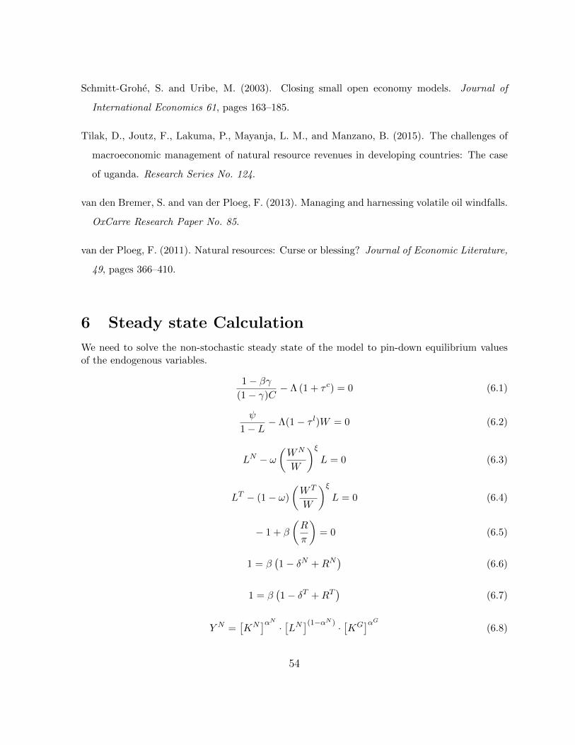
Schmitt-Grohe, S. and Uribe, M. (2003). Closing small open economy models. Journal of
International Economics 61, pages 163–185.
Tilak, D., Joutz, F., Lakuma, P., Mayanja, L. M., and Manzano, B. (2015). The challenges of
macroeconomic management of natural resource revenues in developing countries: The case
of uganda. Research Series No. 124.
van den Bremer, S. and van der Ploeg, F. (2013). Managing and harnessing volatile oil windfalls.
OxCarre Research Paper No. 85.
van der Ploeg, F. (2011). Natural resources: Curse or blessing? Journal of Economic Literature,
49, pages 366–410.
6 Steady state Calculation
We need to solve the non-stochastic steady state of the model to pin-down equilibrium valuesof the endogenous variables.
1− βγ(1− γ)C
− Λ (1 + τ c) = 0 (6.1)
ψ
1− L − Λ(1− τ l)W = 0 (6.2)
LN − ω(WN
W
)ξL = 0 (6.3)
LT − (1− ω)
(W T
W
)ξL = 0 (6.4)
− 1 + β
(R
π
)= 0 (6.5)
1 = β(1− δN +RN
)(6.6)
1 = β(1− δT +RT
)(6.7)
Y N =[KN
]αN · [LN](1−αN ) ·[KG]αG
(6.8)
54
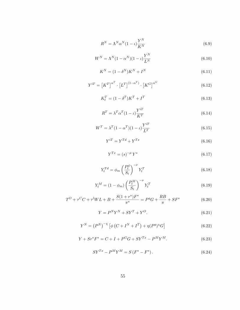
RN = ΛNαN (1− ι)YN
KN(6.9)
WN = ΛN (1− αN )(1− ι)YN
LN(6.10)
KN = (1− δN )KN + IN (6.11)
Y iT =[KT]αT · [LT ](1−αT ) ·
[KG]αG
(6.12)
KTt = (1− δT )KT + IT (6.13)
RT = λTαT (1− ι)YiT
KT(6.14)
W T = λT (1− αT )(1− ι)YiT
LT(6.15)
Y iT = Y Td + Y Tx (6.16)
Y Tx = (s)−µ Y ∗ (6.17)
Y Tdt = φm
(P dtSt
)−νY Tt (6.18)
YMt = (1− φm)
(PMtSt
)−νY Tt (6.19)
TO + τCC + τ lWL+B +S(1 + r∗)F ∗
π∗= P gG+
RB
π+ SF ∗ (6.20)
Y = PNY N + SY T + Y O. (6.21)
Y N =(PN)−χ [
φ(C + IN + IT
)+ η(P g)χG
](6.22)
Y + Sr∗F ∗ = C + I + PGG+ SY Tx − PMYM . (6.23)
SY Tx − PMYM = S (F ∗ − F ∗) . (6.24)
55
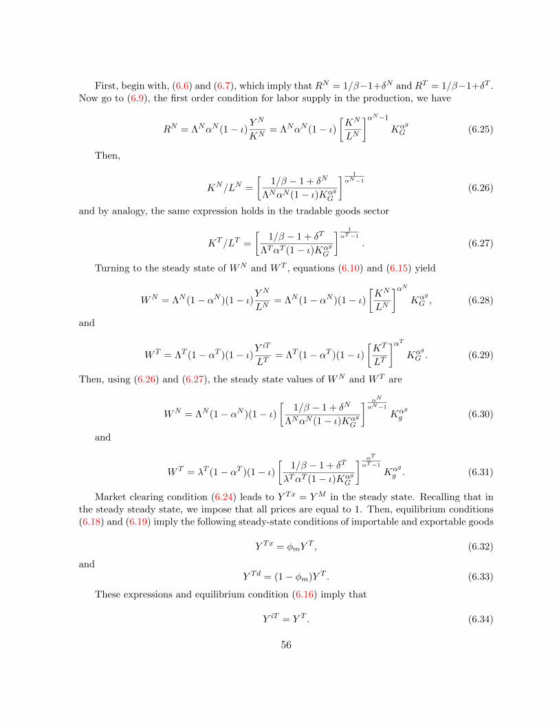
First, begin with, (6.6) and (6.7), which imply that RN = 1/β−1+δN and RT = 1/β−1+δT .Now go to (6.9), the first order condition for labor supply in the production, we have
RN = ΛNαN (1− ι)YN
KN= ΛNαN (1− ι)
[KN
LN
]αN−1
Kαg
G (6.25)
Then,
KN/LN =
[1/β − 1 + δN
ΛNαN (1− ι)KαgG
] 1
αN−1
(6.26)
and by analogy, the same expression holds in the tradable goods sector
KT /LT =
[1/β − 1 + δT
ΛTαT (1− ι)KαgG
] 1
αT−1
. (6.27)
Turning to the steady state of WN and W T , equations (6.10) and (6.15) yield
WN = ΛN (1− αN )(1− ι)YN
LN= ΛN (1− αN )(1− ι)
[KN
LN
]αNKαg
G , (6.28)
and
W T = ΛT (1− αT )(1− ι)YiT
LT= ΛT (1− αT )(1− ι)
[KT
LT
]αTKαg
G . (6.29)
Then, using (6.26) and (6.27), the steady state values of WN and W T are
WN = ΛN (1− αN )(1− ι)[
1/β − 1 + δN
ΛNαN (1− ι)KαgG
] αN
αN−1
Kαg
g (6.30)
and
W T = λT (1− αT )(1− ι)[
1/β − 1 + δT
λTαT (1− ι)KαgG
] αT
αT−1
Kαg
g . (6.31)
Market clearing condition (6.24) leads to Y Tx = YM in the steady state. Recalling that inthe steady steady state, we impose that all prices are equal to 1. Then, equilibrium conditions(6.18) and (6.19) imply the following steady-state conditions of importable and exportable goods
Y Tx = φmYT , (6.32)
andY Td = (1− φm)Y T . (6.33)
These expressions and equilibrium condition (6.16) imply that
Y iT = Y T . (6.34)
56
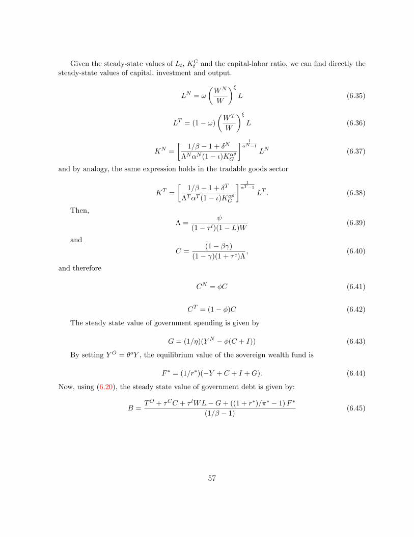
Given the steady-state values of Lt, KGt and the capital-labor ratio, we can find directly the
steady-state values of capital, investment and output.
LN = ω
(WN
W
)ξL (6.35)
LT = (1− ω)
(W T
W
)ξL (6.36)
KN =
[1/β − 1 + δN
ΛNαN (1− ι)KαgG
] 1
αN−1
LN (6.37)
and by analogy, the same expression holds in the tradable goods sector
KT =
[1/β − 1 + δT
ΛTαT (1− ι)KαgG
] 1
αT−1
LT . (6.38)
Then,
Λ =ψ
(1− τ l)(1− L)W(6.39)
and
C =(1− βγ)
(1− γ)(1 + τ c)Λ, (6.40)
and therefore
CN = φC (6.41)
CT = (1− φ)C (6.42)
The steady state value of government spending is given by
G = (1/η)(Y N − φ(C + I)) (6.43)
By setting Y O = θoY , the equilibrium value of the sovereign wealth fund is
F ∗ = (1/r∗)(−Y + C + I +G). (6.44)
Now, using (6.20), the steady state value of government debt is given by:
B =TO + τCC + τ lWL−G+ ((1 + r∗)/π∗ − 1)F ∗
(1/β − 1)(6.45)
57