optical tomography in the presence of void regions · optical tomography in the presence of void...

Dehghani et al. Vol. 17, No. 9 /September 2000 /J. Opt. Soc. Am. A 1659

Optical tomography in the presenceof void regions

Hamid Dehghani

Department of Medical Physics and Bioengineering, University College London, 11-20 Capper Street,London WC1E 6JA, United Kingdom

Simon R. Arridge and Martin Schweiger

Department of Computer Science, University College London, Gower Street, London, WC1E 6BT, United Kingdom

David T. Delpy

Department of Medical Physics and Bioengineering, University College London, 11-20 Capper Street,London WC1E 6JA, United Kingdom

Received November 11, 1999; accepted April 18, 2000

There is a growing interest in the use of near-infrared spectroscopy for the noninvasive determination of theoxygenation level within biological tissue. Stemming from this application, there has been further research inthe use of this technique for obtaining tomographic images of the neonatal head, with the view of determiningthe levels of oxygenated and deoxygenated blood within the brain. Owing to computational complexity, meth-ods used for numerical modeling of photon transfer within tissue have usually been limited to the diffusionapproximation of the Boltzmann transport equation. The diffusion approximation, however, is not valid inregions of low scatter, such as the cerebrospinal fluid. Methods have been proposed for dealing with nonscat-tering regions within diffusing materials through the use of a radiosity-diffusion model. Currently, this newmodel assumes prior knowledge of the void region location; therefore it is instructive to examine the errorsintroduced in applying a simple diffusion-based reconstruction scheme in cases in which there exists a non-scattering region. We present reconstructed images of objects that contain a nonscattering region within adiffusive material. Here the forward data is calculated with the radiosity-diffusion model, and the inverseproblem is solved with either the radiosity-diffusion model or the diffusion-only model. The reconstructedimages show that even in the presence of only a thin nonscattering layer, a diffusion-only reconstruction willfail. When a radiosity-diffusion model is used for image reconstruction, together with a priori informationabout the position of the nonscattering region, the quality of the reconstructed image is considerably improved.The accuracy of the reconstructed images depends largely on the position of the anomaly with respect to thenonscattering region as well as the thickness of the nonscattering region. © 2000 Optical Society of America[S0740-3232(00)00809-7]

OCIS codes: 170.3660, 290.1990, 100.3010.

1. INTRODUCTIONOptical tomography is a new noninvasive imaging tech-nique that aims to image the optical properties of biologi-cal tissue, particularly the peripheral muscle, the breast,and the brain.1–15 See Refs. 16–18 for recent detailed re-views of the state of the art. An optode placed on the sur-face of the region of interest will deliver an input signal(either continuous-wave, amplitude-modulated or ul-trashort pulses of photons), while other optodes placed atdifferent locations on the same surface will detect the out-coming photons that have propagated through the volumeunder investigation. The intensity and the path-lengthdistribution of the exiting photons provides informationabout the optical properties of the transilluminated tis-sue.

The optical properties of tissue vary considerably overa range of wavelengths. The characteristic tissue scatteris commonly expressed in terms of the reduced scatter co-efficient ms8 5 ms(1 2 g), where g is the mean cosine ofthe single-scatter function (the anisotropy factor) and ms

0740-3232/2000/091659-12$15.00 ©

is the scatter coefficient. For biological tissue the valueof g is usually ;0.9, which describes a mainly forwardscatter for the tissue. Typically at 800 nm ms8 is ;1–2mm21 for breast and neonatal brain tissue and is largerfor muscle and adult brain.19,20 The other major opticalproperty of concern is the absorption coefficient ma , whichat 800 nm is approximately 0.01–0.025 mm21 for softtissue20 but generally increases with wavelength, sincethe dominant component in most soft tissue is water.However, very strong absorption from hemoglobin inblood at wavelengths less than 600 nm limits the wave-length range of the radiation that can be used for imagingthrough several centimeters of tissue to the red and nearinfrared (NIR) region.16

Numerical modeling of light propagation in scatteringtissue has become well established in optical tomographylargely through the use of the diffusion approximation tothe Boltzmann transport equation.21–23 The diffusionapproximation is, however, valid only for materials thatare much more scattering than absorbing. This may be

2000 Optical Society of America

1660 J. Opt. Soc. Am. A/Vol. 17, No. 9 /September 2000 Dehghani et al.

suitable for measurements involving largely scatteringmedia, for example, the female breast or peripheralmuscle. Our major interest in optical tomography, how-ever, lies in its use for the imaging of the neonatal head.In such studies the aim would be to detect changes in theoxygenation state of specific regions of the brain as an aidto the understanding and prevention of cerebral handi-cap. Within the head there are regions that are nonscat-tering while still absorbing, namely, the cerebrospinalfluid (CSF) layer around the brain and in the ventricles.The presence of CSF prevents the accurate modeling ofphoton propagation within the regions of interest whenthe diffusion approximation24 is used.

Our aim in this study is to investigate the effect of arelatively simple nonscattering region on images recon-structed with a diffusion-based model and in particular tosimulate the case of the CSF-filled regions within the neo-natal head.

2. FORWARD PROBLEMWe have modeled a nonscattering region within a diffus-ing medium using a new radiosity-diffusion model.25

Under the assumption that scattering dominates absorp-tion in a region of interest, the Boltzmann transport equa-tion can be simplified to the diffusion approximation,which in the frequency domain is given by

2¹ • k~r!¹F~r, v! 1 S ma 1iv

c DF~r, v! 5 q0~r, v!,

(1)

where q0(r, v) is an isotropic source and F(r, v) is thephoton density at position r. The diffusion coefficient k isgiven by

k 51

3~ma 1 ms8!. (2)

Theoretical and experimental results have so far dem-onstrated the validity of these equations under appropri-ate conditions, where ms8 @ ma .26–28

Within a clear nonscattering region, photon migrationcan be calculated with the radiosity theory.29 Thistheory simply calculates the irradiance of a surface from alight source at a given point and angle. In the case of aclear layer having an absorption coefficient ma , the irra-diance at a point r2 on a surface G2 due to a source r1 onanother surface G1 is given as

G2i ~r2! 5

I1~r1!cos~u1!cos~u2!

ur1 2 r2u2

3 exp@2ur1 2 r2u~ma 1 iv/c !#, (3)

where I1 is the source strength from point r1 on surfaceG1 . ur1 2 r2u represents the distance between the twopoints. u1 is the angle between the source vector frompoint r1 and the normal at point r1 , and u2 is the anglebetween the source vector at point r2 and the normal atpoint r2 .

This radiosity-diffusion method for calculating photonpropagation in diffusing tissue containing nonscatteringregions has shown a very good agreement with models of

the Boltzmann transport equation, Monte Carlo models,and with experimental results.25,30,31

3. INVERSE PROBLEM: IMAGERECONSTRUCTIONA. Image Reconstruction in the Absence of VoidsWe assume that the data, y, are represented by a nonlin-ear operator, F,

yM 5 FM@ma , k#, (4)

where M represents a measurement type.32 Then theimage-reconstruction method seeks a solution,

~m̂a , k̂ ! 5 arg minma ,k@ iyM 2 FM~ma , k!iR 1 C~ma , k!#,(5)

where i • iR is the weighted L2 norm, R is the inverse ofthe data covariance matrix, and C is a functional repre-senting prior knowledge.

We use a finite-element method (FEM) as a general andflexible method for solving the forward problem in arbi-trary geometries. As developed in Refs. 21 and 22, givena domain V, bounded by ]V, Eq. (1) is expressed in theFEM framework as

@K~k! 1 C~m! 1 zA 1 ivB#F~v! 5 q0~v!, (6)

where z is a constant depending on the refractive-indexmismatch at the air–tissue boundary, and the system ma-trices K, C, A, and B have entries given by

Kij 5 EV

k~r!¹ui~r! • ¹uj~r!dnr, (7)

Cij 5 EV

ma~r!ui~r!uj~r!dnr, (8)

Bij 51

cE

Vui~r!uj~r!dnr, (9)

Aij 5 E]V

ui~r!uj~r!dn21r, (10)

where ui is the shape function associated with node i ofthe FEM mesh, and F(v), q0(v) are vectors representingthe field and the source, respectively, at the nodal pointsat the mesh.

The modeled data is obtained by application of a mea-surement operator:

yM 5 M@F#. (11)

Our approach has been to use measurement operatorsof a normalized integral transform type, which can be ef-ficiently calculated directly from Eq. (1) without explicitlysolving the parabolic time-domain version of theproblem.33,34 This approach reduces the cost of the for-ward model by an order of magnitude. In this paper weuse only the mean time (i.e., the first moment of the tem-poral response function), although other data types maygive improved results.35

We assume that ma(r) and k(r) are expressed in a basiswith a limited number of dimensions (less than the di-mension of the finite-element-system matrices). A num-


ber of different strategies for defining reconstructionbases are possible36; in this paper we use a regular bilin-ear pixel basis.

To find (m̂a ,k̂) in Eq. (5), we originally proposed aLevenberg–Marquardt algorithm,37 although in this pa-per we use the more efficient gradient-based algorithmdescribed in Ref. 38.

B. Image Reconstruction in the Presence of VoidsThe above mechanism is easily modified to the case inwhich the domain V contains nonscattering void regions.We have a domain V consisting of R diffusing regions$V1 ,V2 ,..., VR% and V void regions $V̄1 ,V̄2 ,..., V̄V%. LetVd 5 ø i51

R V i be the union of all diffusing regions andV̄d 5 ø i51

V V̄i be the union of all void regions. Thus V

5 Vd ø V̄d. The forward problem Eq. (6) has an addi-tional coupling term added for each void, to give

@K~k! 1 C~m! 1 zA 1 ivB 2 E~v!#F~v! 5 q0~v!, (12)

where the new term E(v) is assembled from componentmatrices for each void region, with entries given by

Eij 5 zEAi

ui~r1!EAj

uj~r2!h~r1 , r2!cos~u1!cos~u2!

ur1 2 r2u2

3 exp 2 @ ur1 2 r2u~ma 1 iv/c !#dn21r2dn21r1 ,

(13)

where h(r1 , r2) is a binary function having value 1 ifpoints r1 and r2 are mutually visible. A more detaileddescription of the radiosity-diffusion method can be foundin Ref. 25.

The gradient of the objective function is obtained in thesame way as before, with Eq. (12) instead of Eq. (6) forboth the forward and the adjoint field calculations. Allother components of the algorithm remain unchanged.

4. METHOD AND RESULTSIn the following examples, several different forward mod-els are used to generate data. In each case a two-dimensional circular model of radius 35 mm is used, with16 sources and detectors placed equidistant on the outerboundary. The sources were modeled as an isotropicpoint source, placed one scattering distance (0.5 mm) in-side the outer boundary, and a Robin boundary conditionwas used.22 Only the mean time of flight was consideredas the data type.

Images were reconstructed from this data using twomodels:

1. A diffusion-only model in which no clear nonscat-tering regions were considered. No a priori knowledge ofthe nonscattering region is used here, such as simply witha low ms8 value in the known region, because such an ap-proximation, although possible in the diffusion-onlymodel, is an inadequate description of the actual lightpropagation.25,30

2. A radiosity-diffusion model with correct a priori in-formation about the position, size, and refractive-indexproperties of the nonscattering region.

Regularization in the form of Markov random field wasused in all reconstructions.35,39 We add Markov randomfield terms of the form

C~ p ! 5 (i51

D

(j51

nn~i !

l~ p !upi 2 pn~i, j !ua (14)

to the objective function in Eq. (5), where D is the totalnumber of nodes in the model, pi is the solution at node i,for p either ma or k. nn(i) is the total number of neigh-bors to i with n(i, j) being the jth neighbor of node i.l ( p) is a hyperparameter for each solution parameter.The value of l ( p) is chosen automatically for each case byuse of the Miller criterion.40

The exact characteristics of the models, including meshsizes, numbers of sources and detectors, the source model,regularization parameters, reconstruction bases, and theinverse algorithm, were made as far as possible identicaland are tabulated in Table 1. In each case, only ma im-ages are considered.

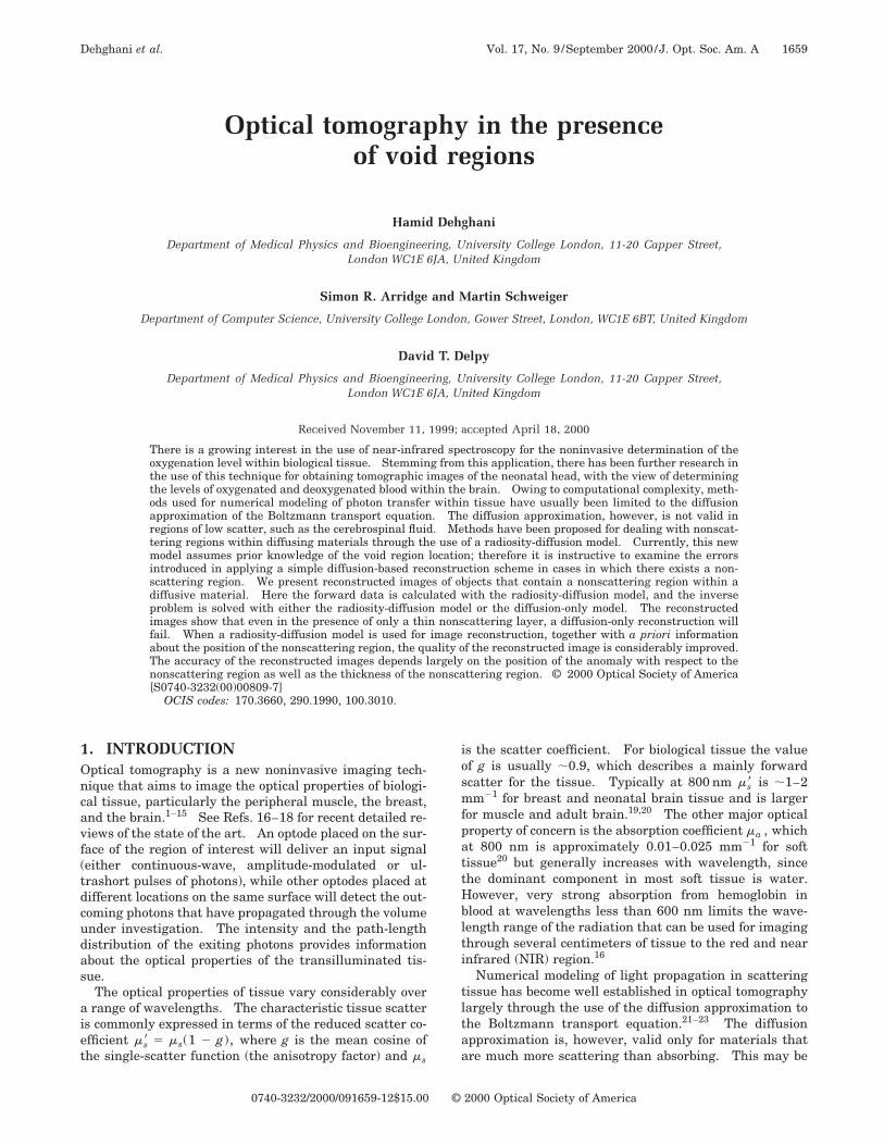
A. Case 1: Nonscattering VoidThe first case considered is a concentric nonscattering cir-cular region of radius 10 mm [Fig. 1(a)]. The backgroundoptical properties of the diffusing region were set as ms85 2 mm21, ma 5 0.01 mm21, and a refractive index of1.4. The nonscattering central region had an absorptionvalue of ma 5 0.005 mm21 and a refractive index of 1.4.A Gaussian anomaly of full width half-maximum(FWHM) 6 mm was placed at 20 mm above the center,with the same scattering and refractive-index propertiesas the background and a peak absorption value of ma5 0.02 mm21.

Reconstructed images at the 100th iteration of the con-jugate gradient solver are shown in Figs. 1(b) and 1(c).From the image in Fig. 1(b) it can be seen that the modelbased solely on the diffusion approximation fails to recon-struct a useful image. The image reconstructed with theradiosity-diffusion model [Fig. 1(c)] appears far more suc-cessful and has reconstructed a very clear and sharp im-age of the internal absorption distribution of the forwardmodel. The average calculated background ma of themodel is approximately 0.01 mm21, and the maximum maof the anomaly is 0.02143 mm21.

Table 1. Definition of Parameters in Models

Parameter Diffusion Model Radiosity-Diffusion Model

Forward Mesh 2825 nodes, 5478elements

2922 nodes, 5372 elements

Inverse Mesh 2825 nodes, 5478elements

2922 nodes, 5372 elements

Basis Pixels 20 3 20 Pixels 20 3 20Filtering Median at each

iterationMedian at each iteration

Regularization MRF a a 5 1.1 MRF a a 5 1.1No. Iterations 100 100

a Markov random field.


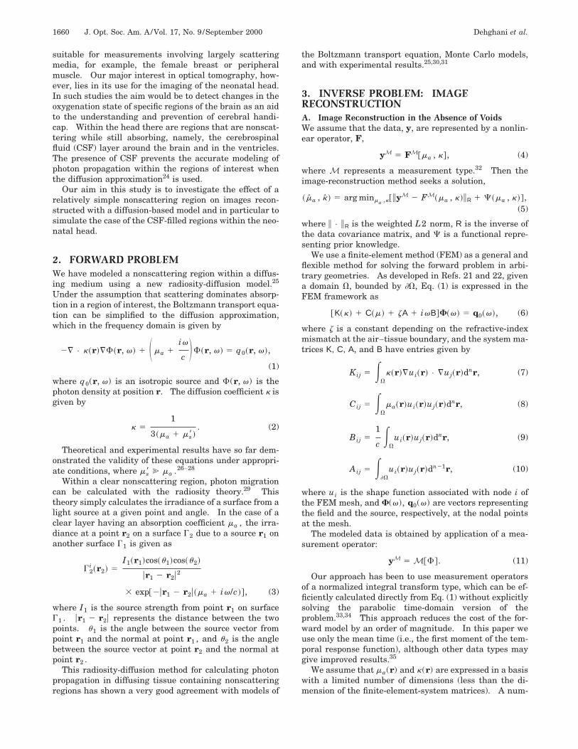
B. Case 2: Nonscattering GapNext, a concentric 2-mm-thick annular nonscattering re-gion extending from a radius of 10 to 12 mm within thediffusing region was modeled [Fig. 2(a)]. The back-ground optical properties of the diffusing region and theabsorption and refractive-index properties of the nonscat-tering ring were set as in the previous model. A Gauss-ian anomaly with the amplitude, FWHM, and location ofthe previous case was again modeled. Forward data was

Fig. 1. (a) Outline of the model (radius 5 35 mm) used for theco-centrally placed circular nonscattering region (radius5 10 mm). The optical properties of the diffusion region arems8 5 2 mm21, ma 5 0.01 mm21, and refractive index 5 1.4.For the nonscattering region, ma 5 0.005 mm21 and refractiveindex 5 1.4. A circular anomaly (blob of radius 5 3 mm) wasmodeled within the diffusing region with ms8 5 2 mm21 and ma5 0.02 mm21. (b) Reconstructed image with a diffusion-onlymodel. (c) Reconstructed image with a radiosity-diffusionmodel.

calculated as before, and ma images were reconstructedwith the two different methods.

Reconstructed images at the 100th iteration of theconjugate-gradient solver are shown in Figs. 2(b) and 2(c).From the image in Fig. 2(b) it can be seen that the modelbased solely on the diffusion approximation again fails toreconstruct a useful image. Image reconstructed withthe radiosity-diffusion model [Fig. 2(c)] appears far moresuccessful and has reconstructed a clear and sharp image

Fig. 2. (a) Outline of the model (radius 5 35 mm) used. Thenonscattering annular region is 2-mm thick at a radius extend-ing from 10 to 12 mm. The optical properties of the diffusionregion are ms8 5 2 mm21, ma 5 0.01 mm21, and refractiveindex 5 1.4. For the nonscattering region, ma 5 0.005 mm21

and refractive index 5 1.4. A circular anomaly (blob of radius5 3 mm) was modeled within the diffusing region with ms85 2 mm21 and ma 5 0.02 mm21. (b) Reconstructed image witha diffusion-only model. (c) Reconstructed image with aradiosity-diffusion model.


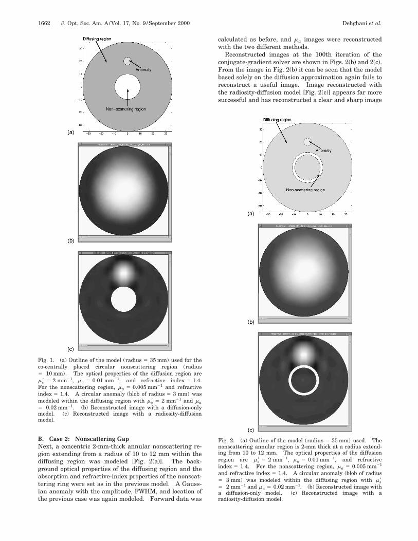
Fig. 3. (a) Outline of the model (radius 5 35 mm) used. The nonscattering annular region has a thickness of 1–4 mm, at a radius of28–32 mm. The optical properties of the diffusion region are ms8 5 2 mm21, ma 5 0.01 mm21, and refractive index 5 1.4. For thenonscattering region, ma 5 0.005 mm21 and refractive index 5 1.4. A circular anomaly (blob of radius 5 3 mm) was modeled withinthe diffusing region with ms8 5 2 mm21 and ma 5 0.04 mm21. (b)–(e) Reconstructed images with a diffusion-only model for the 1–4 mmnonscattering region. (f )–(i) Reconstructed images with a radiosity-diffusion model for the 1–4 mm nonscattering region.

of the internal absorption distribution of the forwardmodel. The average calculated background ma of themodel is approximately 0.01 mm21, and the maximum maof the anomaly is 0.02107 mm21.

C. Case 3: Variable Gap ThicknessTo simulate the case of the CSF ring within the neonatehead, a concentric nonscattering gap was placed at a dis-tance of 3 mm from the outer boundary of the diffusingmodel [Fig. 3(a)], with its thickness varying from 1 to 4mm. The optical properties of the diffusing and nondif-fusion regions were as in the previous cases. A Gaussiananomaly with the same properties as before was placedwithin the central part of the diffusing region as shown inFig. 3(a).

From the images in Figs. 3(b)–3(e) it can be seen thatthe models based solely on the diffusion approximationagain fail to reconstruct a useful image. It has been pre-viously reported that for data from a model containing aCSF ring thickness of greater than 0.5 mm the diffusionapproximation fails to reconstruct.41 However, the pre-vious study was restricted to only time-independent data,and therefore only photon intensity was used.

The images reconstructed with the radiosity-diffusionmodel are not as expected [Fig. 3(f )–3(i)]. From the pre-vious cases shown, it is reasonable to expect the quality of

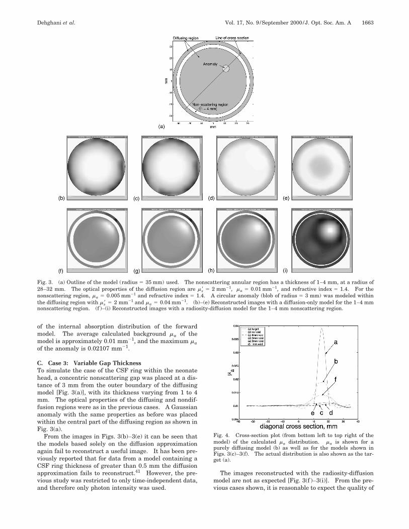
Fig. 4. Cross-section plot (from bottom left to top right of themodel) of the calculated ma distribution. ma is shown for apurely diffusing model (b) as well as for the models shown inFigs. 3(c)–3(f). The actual distribution is also shown as the tar-get (a).


reconstructed images to be as good in this case as the pre-vious cases. The only major difference here is that theanomaly is placed within the clear annular ring. Also,when dealing with purely diffusive material, one can de-tect a single anomaly can quite easily and very clearlywith similar methods. The reconstructed images showthat the quality is not as good if the thickness of the an-nular ring is greater than 1 mm. Figure 4 shows a cross-section plot (from bottom left to top right of the model) ofthe calculated ma distribution for each model, as well asthe target distribution and the calculated distribution ob-tained if no clear layer was present in the forward and theinverse models. It is found that, as the thickness of theclear annular layer becomes larger, the calculated ma ofthe anomaly becomes worse. Also, for the thicker layersof the nonscattering region, the peak value of the anomalyis seen to move nearer to the boundary of the model.

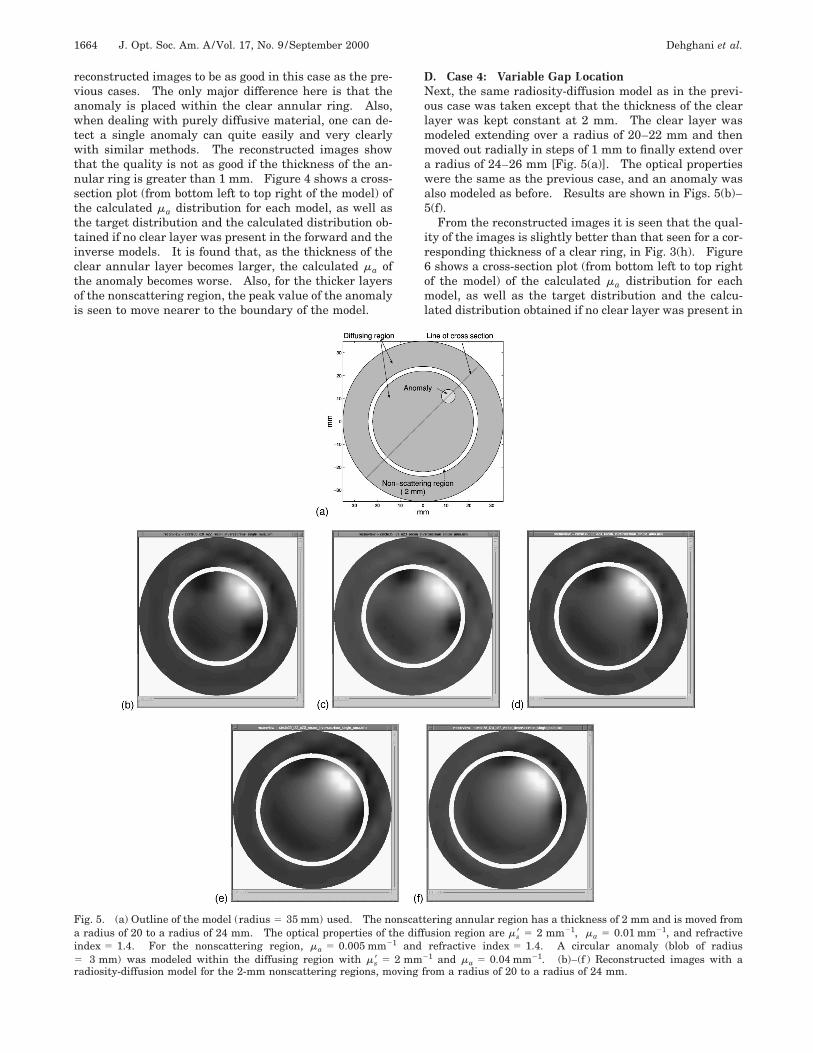
D. Case 4: Variable Gap LocationNext, the same radiosity-diffusion model as in the previ-ous case was taken except that the thickness of the clearlayer was kept constant at 2 mm. The clear layer wasmodeled extending over a radius of 20–22 mm and thenmoved out radially in steps of 1 mm to finally extend overa radius of 24–26 mm [Fig. 5(a)]. The optical propertieswere the same as the previous case, and an anomaly wasalso modeled as before. Results are shown in Figs. 5(b)–5(f).

From the reconstructed images it is seen that the qual-ity of the images is slightly better than that seen for a cor-responding thickness of a clear ring, in Fig. 3(h). Figure6 shows a cross-section plot (from bottom left to top rightof the model) of the calculated ma distribution for eachmodel, as well as the target distribution and the calcu-lated distribution obtained if no clear layer was present in

Fig. 5. (a) Outline of the model (radius 5 35 mm) used. The nonscattering annular region has a thickness of 2 mm and is moved froma radius of 20 to a radius of 24 mm. The optical properties of the diffusion region are ms8 5 2 mm21, ma 5 0.01 mm21, and refractiveindex 5 1.4. For the nonscattering region, ma 5 0.005 mm21 and refractive index 5 1.4. A circular anomaly (blob of radius5 3 mm) was modeled within the diffusing region with ms8 5 2 mm21 and ma 5 0.04 mm21. (b)–(f ) Reconstructed images with aradiosity-diffusion model for the 2-mm nonscattering regions, moving from a radius of 20 to a radius of 24 mm.


the forward and the inverse models. It is seen from thecross section that when the nonscattering ring is at a sub-stantial depth within the diffusing model (15 mm) and theanomaly is positioned near the edge of the clear layer, thereconstructed ma distribution appears best. As the clearlayer is moved out radially, the quality and quantitativevalue of the reconstructed ma distribution become worse.

E. Case 5: Comparison of Image Quality with andwithout a Nonscattering GapFor the next stage of the study, both a purely diffusivemodel and a model with a 2-mm-thick clear layer extend-ing over a radius of 26–28 mm were compared. Thesame Gaussian anomaly was placed at the center of themodel and moved out radially in 11 equal steps until itwas centered at a radius of 28.28 mm. Images are shownfor each position of the anomaly in Figs. 7(a)–7(k) for thediffusion-only case and in Figs. 8(a)–8(k) for the clear-gapcase. In this example, only the radiosity-diffusion modelis used in the inverse solver for the gap case, since the dif-fusion model fails, as has been shown in the previousthree cases.

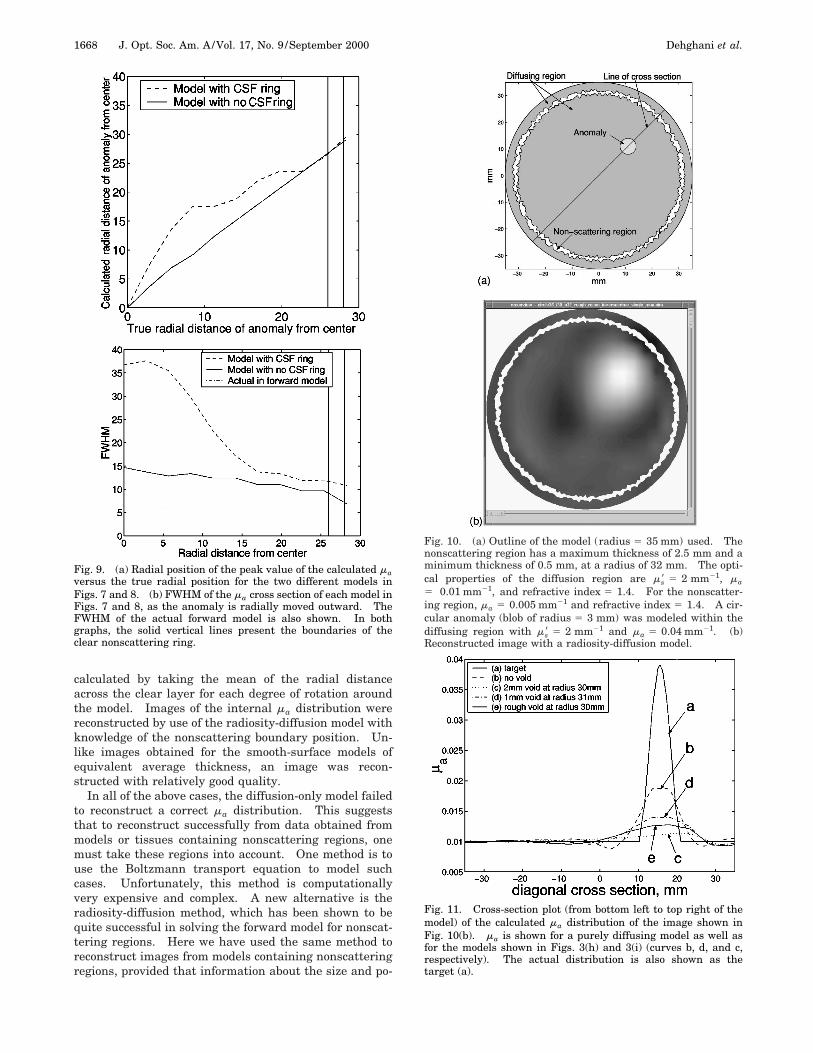
To allow better comparison, the radial peak position ofthe anomaly, in each case with use of the two models, wascalculated by taking the position of the peak value of thecalculated ma distribution, and these are shown in Fig.9(a). It can be seen from this graph that in the purelydiffusing model, the calculated position of the anomaly isvery good compared with its actual position. Theradiosity-diffusion model, however, shows a very nonlin-ear response. When the anomaly is positioned deep in-side the model (0–7 mm), the calculated peak position isnot very good compared with the actual. Between a ra-dius of 7 and 12 mm, the calculated peak position does notchange by a large amount. The calculated peak positionof the anomaly becomes more accurate only when its ac-tual position is nearest to the inner edge of the clear ringand also when the anomaly is placed outside the clearring.

Fig. 6. Cross-section plot (from bottom left to top right of themodel) of the calculated ma distribution. ma is shown for apurely diffusing model as well as the model shown in Fig. 5.The actual distribution is also shown as the target.

To look further at the effect of this 2-mm-thick clearlayer in the model, we calculated the FWHM for the crosssection of the calculated absorption of the anomaly ineach of the models (with and without the 2-mm clearlayer); the results are shown in Fig. 9(b). The line rep-resenting the calculated FWHM of the purely diffusingmodel (solid curve) is as expected. This shows that asthe anomaly gets nearer the boundary of the model, thereconstructed images become better and sharper becausethe sensitivity in these regions is higher than those in thecenter of the model.42 The other notable feature of thecalculated FWHM is that the area of the reconstructedanomaly is shown to be much greater than the estimatedarea, at a radius of less than 15 mm from the center of themodel. This is also evident from the reconstructed im-ages shown in Fig. 8.

A notable feature of the reconstructed images shown inFig. 8 is that as the anomaly moves nearer the edge of theclear nonscattering ring, the reconstructed shape of theanomaly becomes more elongated along the edge of thenonscattering ring. Again this can be due to the highsensitivity of the regions nearer to the edge of the non-scattering ring.

F. Case 6: Irregular Gap ThicknessA final model was constructed in which the clear layerhas an irregular boundary [Fig. 10(a)]. This model hasbeen included, since in reality the CSF layer around thebrain is indeed irregular. It has also been suggested30

that the profound effect of the clear layer is due to the ex-tended ‘‘line of sight’’ for the photons crossing this region,which would be more limited if the boundary were irregu-lar. The irregular boundary was calculated by addingnoise to the x and y coordinates of the smooth boundaryand then smoothing to a desired level by removing thehigher-frequency roughness. In this model the maxi-mum thickness of the nonscattering ring is 2.5 mm andthe minimum is ;0.5 mm. The optical properties werethe same as the previous case, and an anomaly was alsomodeled as previously. Images of ma distribution werereconstructed with only the radiosity-diffusion model(with the correct a priori information about the positionand size of the nonscattering region). The 100th itera-tion of the conjugate-gradient algorithm is shown in Fig.10(b). From the reconstructed image as well as thecross-section plot of the calculated absorption distributionin Fig. 11, it can be seen that the quality of the recon-structed image is much better than that of a correspond-ing 2-mm smooth-surfaced clear ring [Fig. 3(h)] and al-most as good as that of the 1-mm-thick clear ring [Fig.3(i)].

5. DISCUSSION AND CONCLUSIONSForward solutions of diffusion-based models that containnonscattering regions have been calculated with theradiosity-diffusion finite-element method. Data fromthese forward solutions were then used to reconstruct im-ages of internal ma distribution with either a diffusion ora radiosity-diffusion model. In the radiosity-diffusionmodel, the position and size of the nonscattering regionhave to be known a priori.


Fig. 7. Reconstructed images of a diffusion-only model where the anomaly is displaced radially from the center of the model (a) to aradius of 28 mm (k) in 11 equal steps.

In cases 1 and 2 we show that in the presence of asingle nonscattering region (circular or annular), if theanomaly is located outside the clear region, an accurateimage of the internal ma distribution can be calculated.In these cases, the success of the reconstruction may bedue to the fact that the migrating photons encounter theanomaly before they encounter the nonscattering region.Also, in some cases of source–detector combinations (e.g.,adjacent), the propagating photons may not even encoun-ter a nonscattering region.

Case 3, with a variable gap thickness, showed that,providing the thickness of this nonscattering ring is ;1mm, a good image of the internal ma can be reconstructedwith the radiosity-diffusion model. However, the recon-structed image deteriorates rapidly as the thickness of

the clear layer increases. One possible explanation forthis is that for larger thickness of nonscattering regions,the light entering the clear region from the outer surfacewill illuminate a larger surface on the inner boundary.This results in a more uniform distribution of the light, sothat the light arriving at any detector would provide lessinformation about local inhomogeneities. Furthermore,for large thicknesses of the nonscattering rings, somephotons may even travel around the nonscattering rings,arriving at the detector without having sampled the inte-rior at all.43

For a given thickness of a clear ring (2 mm) that wasmoved from a radius of 20 mm to 24 mm within the model(case 4) it was found that better images of the internal madistribution were reconstructed when the clear layer was


at the maximum depth within the diffusing material andalso was placed such that it was near the anomaly. Thisis probably because any incident light on the surface ofthe model will have traveled a large distance before it en-counters the clear layer. Also, when the clear layer is alarge distance within the diffusing medium, the diffusingarea within the clear layer is smaller, reducing theamount of space needing to be sampled by the light. Fur-thermore, reconstruction of the anomaly within the innerboundary of the clear ring appears to be aided if theanomaly is nearer the inner boundary of the clear ring,indicating a high sensitivity in the regions closest to theboundary of the clear layer.

This latter observation is also seen when the singleanomaly is moved radially outward from the center in the

presence of a given fixed clear ring (case 5). The anomalyis best reconstructed when it is positioned outside theouter boundary of the clear ring. But when the anomalyis within the diffusing area enclosed by the clear ring, thebest possible reconstruction is achieved when theanomaly is nearest the inner boundary of the clear layer.In addition, for reconstructed anomalies that are nearerthe edge of the clear nonscattering ring, a more elongatedreconstructed image along the edge of the clear layer isseen. This can be due primarily to the high sensitivity ofthe data to those regions rather than to the regionsdeeper within the model.

The effect of an irregular clear ring has been examined(case 6). The thickness of the ring varied between 0.5and 2.5 mm, with a mean of 1.507 mm. The average was

Fig. 8. Reconstructed images of the radiosity-diffusion model in the presence of a 2-mm clear ring extending from a radius of 26 to aradius of 28 mm. The anomaly is again as in Fig. 7, displaced radially from the center of the model (i) to a radius of 28 mm (xi) in 11equal steps.


calculated by taking the mean of the radial distanceacross the clear layer for each degree of rotation aroundthe model. Images of the internal ma distribution werereconstructed by use of the radiosity-diffusion model withknowledge of the nonscattering boundary position. Un-like images obtained for the smooth-surface models ofequivalent average thickness, an image was recon-structed with relatively good quality.

In all of the above cases, the diffusion-only model failedto reconstruct a correct ma distribution. This suggeststhat to reconstruct successfully from data obtained frommodels or tissues containing nonscattering regions, onemust take these regions into account. One method is touse the Boltzmann transport equation to model suchcases. Unfortunately, this method is computationallyvery expensive and complex. A new alternative is theradiosity-diffusion method, which has been shown to bequite successful in solving the forward model for nonscat-tering regions. Here we have used the same method toreconstruct images from models containing nonscatteringregions, provided that information about the size and po-

Fig. 9. (a) Radial position of the peak value of the calculated maversus the true radial position for the two different models inFigs. 7 and 8. (b) FWHM of the ma cross section of each model inFigs. 7 and 8, as the anomaly is radially moved outward. TheFWHM of the actual forward model is also shown. In bothgraphs, the solid vertical lines present the boundaries of theclear nonscattering ring.

Fig. 10. (a) Outline of the model (radius 5 35 mm) used. Thenonscattering region has a maximum thickness of 2.5 mm and aminimum thickness of 0.5 mm, at a radius of 32 mm. The opti-cal properties of the diffusion region are ms8 5 2 mm21, ma5 0.01 mm21, and refractive index 5 1.4. For the nonscatter-ing region, ma 5 0.005 mm21 and refractive index 5 1.4. A cir-cular anomaly (blob of radius 5 3 mm) was modeled within thediffusing region with ms8 5 2 mm21 and ma 5 0.04 mm21. (b)Reconstructed image with a radiosity-diffusion model.

Fig. 11. Cross-section plot (from bottom left to top right of themodel) of the calculated ma distribution of the image shown inFig. 10(b). ma is shown for a purely diffusing model as well asfor the models shown in Figs. 3(h) and 3(i) (curves b, d, and c,respectively). The actual distribution is also shown as thetarget (a).


sition of the nonscattering region is known. It has beenshown that, provided that the region of interest is outsidea nonscattering ring (or if the clear ring enclosing the re-gion of interest is approximately no thicker than 1.0 mmand has a smooth boundary), a useful image of the inter-nal ma can be reconstructed.

Finally, it has also been shown that if the surface of thenonscattering layer is not smooth but is rough and irregu-lar, satisfactory images can be reconstructed for largerand thicker nonscattering layers. A more thorough in-vestigation of effects of roughness has been put forward.44

In that work the investigators have shown that in the ex-treme limit of void boundary roughness, the model beginsto behave more like a diffusive model rather than onethat contains a void region.

A drawback of the approach as reported here is that theboundary and optical properties of the void region needsto be known a priori. Recently we reported a method forfinding internal boundaries of piecewise constant diffus-ing media,45 and in subsequent publications we hope toreport on an extension of that method to the case of inter-est here, namely, that one or more of the regions is non-scattering.

In all the cases described in this paper, only the meantime of flight has been used for image reconstruction.The use of additional data types for reconstruction mayconsiderably improve the quality of images.

ACKNOWLEDGMENTSWe thank Jorge Ripoll for helpful discussions and VilleKolehmainen for reading the manuscript. Funding hasbeen generously received from the Engineering andPhysical Sciences Research Council and the WellcomeTrust.

REFERENCES1. S. R. Arridge, P. van der Zee, M. Cope, and D. T. Delpy, ‘‘Re-

construction methods for near infrared absorption imag-ing,’’ in Time-Resolved Spectroscopy and Imaging of Tis-sues, B. Chance and A. Katzir, eds., Proc. SPIE 1431, 204–215 (1991).

2. M. A. O’Leary, D. A. Boas, B. Chance, and A. G. Yodh, ‘‘Ex-perimental images of heterogeneous turbid media byfrequency-domain diffusing-photon tomography,’’ Opt. Lett.20, 426–428 (1995).

3. C. P. Gonatas, M. Ishii, J. S. Leigh, and J. C. Schotland,‘‘Optical diffusion imaging using a direct inversionmethod,’’ Phys. Rev. E 52, 4361–4365 (1995).

4. Ch. L. Matson, N. Clark, L. McMackin, and J. S. Fender,‘‘Three-dimensional tumor localization in thick tissue withthe use of diffuse photon-density waves,’’ Appl. Opt. 36,214–220 (1997).

5. X. D. Li, T. Durduran, A. G. Yodh, B. Chance, and D. N.Pattanayak, ‘‘Diffraction tomography for biochemical imag-ing with diffuse-photon density waves,’’ Opt. Lett. 22, 573–575 (1997).

6. S. A. Walker, S. Fantini, and E. Gratton, ‘‘Image recon-struction by backprojection from frequency-domain opticalmeasurements in highly scattering media,’’ Appl. Opt. 36,170–179 (1997).

7. H. Jiang, K. D. Paulsen, U. L. Osterberg, B. W. Pogue, andM. S. Patterson, ‘‘Simultaneous reconstruction of optical ab-sorption and scattering maps in turbid media from near-infrared frequency-domain data,’’ Opt. Lett. 20, 2128–2130(1995).

8. S. B. Colak, D. G. Papaioannou, G. W. t’Hooft, M. B. van derMark, H. Schomberg, J. C. J. Paasschens, J. B. M. Melis-sen, and N. A. A. J. van Asten, ‘‘Tomographic image recon-struction from optical projections in light-diffusing media,’’Appl. Opt. 36, 181–213 (1997).

9. P. N. den Outer, Th. M. Nieuwenhuizen, and A. Lagendijk,‘‘Location of objects in multiple-scattering media,’’ J. Opt.Soc. Am. A 10, 1209–1218 (1993).

10. S. Feng, F. Zeng, and B. Chance, ‘‘Photon migration in thepresence of a single defect: a perturbation analysis,’’ Appl.Opt. 35, 3826–3836 (1995).

11. J. C. Schotland, ‘‘Continuous-wave diffusion imaging,’’ J.Opt. Soc. Am. A 14, 275–279 (1997).

12. S. J. Norton and T. Vo-Dinh, ‘‘Diffraction tomographic im-aging with photon density waves: an explicit solution,’’ J.Opt. Soc. Am. A 15, 2670–2677 (1998).

13. S. A. Walker, D. A. Boas, and E. Gratton, ‘‘Photon densitywaves scattered from cylindrical inhomogeneities: theoryand experiments,’’ Appl. Opt. 37, 1935–1944 (1998).

14. S. Fantini, S. A. Walker, M. A. Franceschini, M. Kaschke,P. M. Schlag, and K. T. Moesta, ‘‘Assessment of the size, po-sition, and optical properties of breast tumor in vivo by non-invasive optical methods,’’ Appl. Opt. 37, 1982–1989 (1998).

15. J. C. Hebden, F. E. W. Schmidt, M. E. Fry, M. Schweiger, E.M. C. Hillman, D. T. Delpy, and S. R. Arridge, ‘‘Simulta-neous reconstruction of absorption and scattering imagesby multichannel measurement of purely temporal data,’’Opt. Lett. 24, 534–536 (1999).

16. J. C. Hebden, S. R. Arridge, and D. T. Delpy, ‘‘Optical im-aging in medicine. I. experimental techniques,’’ Phys.Med. Biol. 42, 825–840 (1997).

17. S. R. Arridge, ‘‘Topical review: optical tomography inmedical imaging,’’ Inverse Probl. 15, R41–R93 (1999).

18. S. R. Arridge and J. C. Hebden, ‘‘Optical imaging in medi-cine. II. Modelling and reconstruction,’’ Phys. Med. Biol.42, 841–853 (1997).

19. P. van der Zee, ‘‘Measurement and modelling of the opticalproperties of human tissue in the near infrared,’’ Ph.D. dis-sertation (University College London, London, 1993).

20. G. Mitic, J. Kolzer, J. Otto, E. Plies, G. Solkner, and W.Zinth, ‘‘Time-gated transillumination of biological tissueand tissuelike phantoms,’’ Opt. Lett. 33, 6699–6710 (1994).

21. S. R. Arridge, M. Schweiger, M. Hiraoka, and D. T. Delpy,‘‘A finite element approach for modeling photon transportin tissue,’’ Med. Phys. 20, 299–309 (1993).

22. M. Schweiger, S. R. Arridge, M. Hiraoka, and D. T. Delpy,‘‘The finite element model for the propagation of light inscattering media: boundary and source conditions,’’ Med.Phys. 22, 1779–1792 (1995).

23. H. Jiang, K. D. Paulsen, U. L. Osterberg, B. W. Pogue, andM. S. Patterson, ‘‘Optical image reconstruction usingfrequency-domain data: simulations and experiments,’’ J.Opt. Soc. Am. A 13, 253–266 (1996).

24. A. H. Hielscher, R. E. Alcouffe, and R. L. Barbour, ‘‘Com-parison of finite-difference transport and diffusion calcula-tions for photon migration in homogeneous and heterog-enous tissue,’’ Phys. Med. Biol. 43, 1285–1302 (1998).

25. S. R. Arridge, H. Dehghani, M. Schweiger, and E. Okada,‘‘The finite element model for the propagation of light inscattering media: a direct method for domains with non-scattering regions,’’ Med. Phys. 27, 252–264 (2000).

26. R. A. J. Groenhuis, H. A. Ferwada, and J. J. Ten Bosch,‘‘Scattering and absorption of turbid materials determinedfrom reflection measurements’’ (parts 1 and 2), Appl. Opt.22, 2456–2467 (1983).

27. T. Nakai, G. Nishimura, K. Yamamoto, and M. Tamura,‘‘Expression of optical diffusion coefficient in high-absorption turbid media,’’ Phys. Med. Biol. 42, 2541–2549(1997).

28. M. Bassani, F. Martelli, G. Zaccanti, and D. Contini, ‘‘Inde-pendence of the diffusion coefficient from absorption: ex-perimental and numerical evidence,’’ Opt. Lett. 22, 853–855 (1997).

29. M. F. Cohen and J. R. Wallace, Radiosity and Realistic Im-age Synthesis (Academic, London, 1993).

30. M. Firbank, S. R. Arridge, M. Schweiger, and D. T. Delpy,


‘‘An investigation of light transport through scattering bod-ies with non-scattering regions,’’ Phys. Med. Biol. 41, 767–783 (1996).

31. J. Ripoll, S. R. Arridge, H. Dehghani, and M. Nieto-Vesperinas, ‘‘Boundary conditions for light propagation indiffusive media with nonscattering regions,’’ J. Opt. Soc.Am. A 17, 1671–1681 (2000).

32. M. Schweiger and S. R. Arridge, ‘‘Optimal data types in op-tical tomography,’’ in Information Processing in MedicalImaging, Lecture Notes in Computer Science, J. Duncanand G. Gindi, eds. (Springer-Verlag, Berlin, 1997), Vol.1230, pp. 71–84.

33. S. R. Arridge and M. Schweiger, ‘‘Direct calculation of themoments of the distribution of photon time of flight in tis-sue with a finite-element method,’’ Appl. Opt. 34, 2683–2687 (1995).

34. S. R. Arridge and M. Schweiger, ‘‘Direct calculation of theLaplace transform of the distribution of photon time offlight in tissue with a finite-element method,’’ Appl. Opt.36, 9042–9049 (1997).

35. M. Schweiger and S. R. Arridge, ‘‘Application of temporalfilters to time-resolved data in optical tomography,’’ Phys.Med. Biol. 44, 1699–1717 (1999).

36. M. Schweiger and S. R. Arridge, ‘‘Optical tomographic re-construction in a complex head model using a priori regionboundary information,’’ Phys. Med. Biol. 44, 2703–2721(1999).

37. M. Schweiger, S. R. Arridge, and D. T. Delpy, ‘‘Applicationof the finite-element method for the forward and inversemodels in optical tomography,’’ J. Math. Imag. Vision 3,263–283 (1993).

38. S. R. Arridge and M. Schweiger, ‘‘A gradient-based optimi-sation scheme for optical tomography,’’ Opt. Express 2,213–226 (1998).

39. J. C. Ye, K. J. Webb, C. A. Bouman, and R. P. Millane, ‘‘Op-tical diffusion tomography by iterative-coordinate-descentoptimization in a Baysian framework,’’ J. Opt. Soc. Am. A16, 2400–2412 (1999).

40. S. R. Arridge, M. Schweiger, M. Hiraoka, and D. T. Delpy,‘‘Performance of an iterative reconstruction algorithm fornear-infrared absorption and scatter imaging,’’ in PhotonMigration and Imaging in Random Media and Tissues, B.Chance, R. R. Alfano, eds., Proc. SPIE 1888, 360–371(1993).

41. H. Dehghani, D. T. Delpy, and S. R. Arridge, ‘‘Photon mi-gration in non-scattering tissue and the effects on image re-construction,’’ Phys. Med. Biol. 44, 2897–2906 (1999).

42. S. R. Arridge and M. Schweiger, ‘‘Photon-measurementdensity functions. Part 2: finite-element-method calcula-tions,’’ Appl. Opt. 34, 8026–8037 (1995).

43. E. Okada and D. T. Delpy, ‘‘The effect of overlaying tissueon NIR light propagation in neonatal brain,’’ Advances inOptical Imaging and Photon Migration, R. R. Alfano and J.G. Fujimoto, eds., Vol. 2 of OSA Trends in Optics and Pho-tonic Series (Optical Society of America, Washington, D.C.,1996), pp. 338–343.

44. J. Ripoll, S. R. Arridge, and M. Nieto-Vesperinas, ‘‘Effect ofroughness in nondiffusive regions within diffusive media,’’manuscript available from J. Ripoll: [email protected].

45. V. Kolehmainen, S. R. Arridge, W. R. B. Lionheart, M.Vauhkonen, and J. P. Kaipio, ‘‘Recovery of region bound-aries of piecewise constant coefficients of an elliptic PDEfrom boundary data,’’ Inverse Probl. 15, 1375–1391 (1999).

optical tomography in the presence of void regions · optical tomography in the presence of void...

Documents