optical properties of gases under extreme conditions ... · astrophysics institute) of the istituto...
TRANSCRIPT

UNIVERSITA DEGLI STUDI DI NAPOLI FEDERICO II
Dottorato di ricerca inIngegneria Aerospaziale, Navale e della Qualita (XXIV Ciclo)
CanditateStefania Stefani
Ph.D. Thesis
Optical properties of gases under planetaryconditions: measurements and models
Tutor: Prof. Pasquale PalumboCo-Tutor: Dr. Giuseppe Piccioni
PhD Coordinator: Ing. Antonio Moccia
Anno Accademico 2010-2011

Contents
Contents i
Introduction 1
1 Remote Sensing data analysis and instrumentation employed 5
1.1 Introduction to the remote sensing technique . . . . . . . . . . . . . . 6
1.2 Remote sensing instruments . . . . . . . . . . . . . . . . . . . . . . . 10
1.3 Radiative transfer processes . . . . . . . . . . . . . . . . . . . . . . . 17
1.4 The Visible and InfraRed Thermal Imaging Spectrometer . . . . . . 20
1.4.1 VIRTIS M . . . . . . . . . . . . . . . . . . . . . . . . . . . . . 23
1.4.2 VIRTIS-H . . . . . . . . . . . . . . . . . . . . . . . . . . . . . 27
1.5 Scientific goals of VIRTIS . . . . . . . . . . . . . . . . . . . . . . . . 31
2 Planetary atmospheres and notions of spectroscopy 35
2.1 Venus . . . . . . . . . . . . . . . . . . . . . . . . . . . . . . . . . . . 36
2.1.1 Venus’s atmosphere . . . . . . . . . . . . . . . . . . . . . . . . 40
2.2 Notions of molecular spectroscopy . . . . . . . . . . . . . . . . . . . . 43
2.2.1 Line shape . . . . . . . . . . . . . . . . . . . . . . . . . . . . 45
2.2.2 Rules to build up a spectrum . . . . . . . . . . . . . . . . . . 49

ii CONTENTS
3 Experimental setup 61
3.1 FT-IR interferometer . . . . . . . . . . . . . . . . . . . . . . . . . . . 61
3.2 Gas cell . . . . . . . . . . . . . . . . . . . . . . . . . . . . . . . . . . 69
3.2.1 Connections and calibrations of the set up . . . . . . . . . . . 74
3.2.2 Measurements procedure . . . . . . . . . . . . . . . . . . . . . 78
4 Radiative transfer models 81
4.1 ARS: Model and Software . . . . . . . . . . . . . . . . . . . . . . . . 82
4.1.1 What does the program do . . . . . . . . . . . . . . . . . . . . 84
4.2 Solution . . . . . . . . . . . . . . . . . . . . . . . . . . . . . . . . . . 87
4.2.1 Line Mixing effect . . . . . . . . . . . . . . . . . . . . . . . . . 87
4.2.2 Far Wings approximation . . . . . . . . . . . . . . . . . . . . 90
4.3 LMM model . . . . . . . . . . . . . . . . . . . . . . . . . . . . . . . 94
4.3.1 Relaxation matrix . . . . . . . . . . . . . . . . . . . . . . . . . 95
4.3.2 Imaginary part of W . . . . . . . . . . . . . . . . . . . . . . . 97
4.3.3 Parameters needed to obtain absorption coefficients . . . . . . 97
5 Results and Discussions 99
5.1 Experimental measurements . . . . . . . . . . . . . . . . . . . . . . . 99
5.2 Comparison between simulated and measured data . . . . . . . . . . 111
5.3 Collision Induced Absorption . . . . . . . . . . . . . . . . . . . . . . 126
5.4 Study of the continuum . . . . . . . . . . . . . . . . . . . . . . . . . . 130
Conclusions 133
Bibliography 137

CONTENTS iii
List of Figures 147
List of Tables 153

Introduction
This work has been completely carried out in the Planetary Laboratory (PLab)
of the Istituto di Astrofisica Spaziale e Fisica cosmica (Cosmic Physics and Space
Astrophysics Institute) of the Istituto Nazionale di AstroFisica (Italian National
Institute for Astrophysics) of Rome. The scientific goals related to this thesis work
are two: implement spectroscopic databases and support the space missions.
Presently a wealth of spectroscopic data are present in several databases, such as
HIgh-resolution- TRANsmission (HITRAN [1]), HIgh-TEMPerature (HITEMP) [2]
Carbon-Dioxide-Spectroscopy-Databank (CDSD [3]). They provides a suite of pa-
rameters of molecular species at typically terrestrial conditions and are routinely
used for the retrieval of many parameters concerning the atmosphere of the Earth.
On the other hand, they not or contain very limited information on the behavior
of gases at extreme conditions, in particular, high pressure and high temperature.
These parameters are of major importance for the radiative transfer models of data
coming from space mission, such VIRTIS (Visible and InfraRed Thermal Imaging
Spectrometer) instrument on board the ESA mission Venus Express [4]. The VIR-
TIS instrument provides hyperspectral images of Venus, in the spectral range from
0.3 to 5.1 micron. The interpretation of these observations requires sophisticated
radiative transfer calculations, based on the spectroscopic knowledge available for

2 Introduction
the main absorber, carbon dioxide. In fact, Venus’ atmosphere, for instance, is much
hotter and denser than the Earth’s, and temperatures up to 450C and pressures
up to 92 bar at the surface have to be considered. The composition is also very
different, being constituted almost entirely of carbon dioxide (97 %). The CO2 is
a strong absorber in the infrared and near infrared part of the spectrum, and the
observation from orbit down to the surface is only possible in the so-called ”trans-
parency windows” in between the strong absorption bands. Despite these needs,
till this moment, accurate experimental and theoretical data for the absorption by
carbon dioxide at high pressure was still missing. For example, in the work [5],
in order to determine the volume mixing ratio profiles of several species in Venus
atmosphere from spectra recorded by VIRTIS instrument, a constant was used for
the CO2 continuum through a wide spectral range.
Laboratory studies of high pressure carbon dioxide absorption are complicated by
different phenomena. Firstly, the widely used Lorentzian line shape strongly over-
estimates the absorption in the band wing regions, while it underestimates the ab-
sorption near band centers at elevated pressure. The second difficulty is linked to
absorption due to the transient dipole moment induced during collisions and/or due
to dimers [or larger (CO2)N clusters] formed in the dense gas. The deviation of
the measured absorption (due to the 3 permanent dipolar moment) with respect to
the Lorentz shape at high pressure is essentially due to collision-induced intensity
transfer between transitions (line-mixing effects) and to the finite duration of inter-
molecular collisions. Several laboratory experimental and theoretical studies were
devoted to high pressure allowed spectra of pure CO2 [6]- [7]. They all point out
the strong discrepancy between the Lorentzian profile and experimental spectra for
the studied spectral region.

3
Thank to the thesis work, numerous data at several temperature, from 294 to 600
K, and pressures, from 1 up to 30 bar, are now available.
This thesis is organized as following: in chapter 1 a brief description of the remote
sensing technique and instrumentation employed are reported. You can find also
an extensive analysis of the VIRTIS spectrometer, which has recorded many images
and spectra of the Venus atmosphere since its orbital insertion, on April 11 2006.
The characteristics of the twin planet of the Earth for dimensions and mass, but
from the behavior a lot different, will be given in chapter 2. Some notions of spec-
troscopy, that gives us a remote access to most of the important information carried
by the radiation which directly interact with the planet, will be introduced in the
second part.
The CO2 absorption coefficients have been measured by a Fourier Transform In-
fraRed (FT-IR) interferometer integrated with a special gas cell. Thanks to this
experimental set-up we can cover a wide spectral range, from 750 to 25000 cm−1
(0.4-29 µm), with a relatively high spectra resolution, from 10 to 0.07 cm−1. Indeed,
the gas cell is designed to support pressure up to 350 bar and temperature up to
650K. A detailed description is reported in the chapter 3.
The measurements have been compared with synthetic spectra obtained using three
different models: one implementing a line by line calculation; the second one taking
into account the line mixing effect in the strong collision approximation and the last
one using a different approach to the line mixing effect. A discussion about this
theoretical model is reported in the chapter 4.

4 Introduction
Finally, in the last chapter (5) a detailed discussion on the measurements ob-
tained using a real vertical venusian profile and the comparison between data and
simulations are reported.
Chapter 1
Remote Sensing data analysis and
instrumentation employed
Undoubtedly, much of what we know about the Solar System comes from direct ex-
ploration. Since the early 1960’s, many robotic spacecrafts have been sent out into
our Solar System to explore and return knowledge and images of distant worlds.
Instrumented probes have descended through the atmosphere of Venus and Mars.
The Mariner, Pioneer, Venera, Viking and Voyager space flight programs have pro-
vided opportunities to study the planets from Mercury to Neptune and most of their
satellites. During this space age, missions of exploration into all the Solar System
have revolutionized our view about the nature of it. Today, we are only at the begin-
ning of this exploration, and even if we have some information, misunderstandings
of many physical phenomena involved are still innumerable. Remote sensing inves-
tigations have been conduced with unprecedented spatial and spectral resolution,
permitting detailed examinations of atmospheres and surfaces. Even for the Earth,
space-borne observations, obtained with global coverage and high spatial, spectral
6 1. Remote Sensing data analysis and instrumentation employed
and temporal resolution, have revolutionized weather forecasting, climate research
and exploration of the natural resources.
The collective study of the various atmospheres and surface in the Solar System con-
stitutes the field of comparative planetology. Wide ranges in surface gravity, solar
flux, internal heat, obliquity, rotation rate, mass and composition provide a broad
spectrum of boundary conditions for atmospheric systems. Analysis of data within
this context lead to an understanding of physical processes applicable to all plan-
ets. Once the general physical principles are identified, the evolution of planetary
system can be explored. Some of the data needed to address the boarder questions
have already been collected. Infrared spectra, images and many other types of data
are available in varying amounts for Mercury, Venus, Earth, Mars, Jupiter, Saturn,
Uranus, Neptune and many of their satellites. It in now appropriate to review and
assess the techniques used in obtaining the existing information. This will not only
provide a summary of our present capabilities, but will also suggest ways of extend-
ing our knowledge to better address the issues of comparative planetology and Solar
System evolution.
The purpose of this chapter is to describe some characteristic of the remote sensing
technique and of the instrumentations employed.
1.1 Introduction to the remote sensing technique
The remote sensing technique, also called remote sounding, employs electromagnetic
radiation reflected, scattered or emitted from the planets or earth atmosphere at a
distance from the observing station. This technique is a powerful tool for investi-
gating the atmospheric structure and composition or surface [8].
1.1 Introduction to the remote sensing technique 7
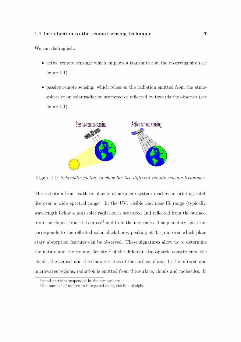
We can distinguish:
• active remote sensing: which employs a transmitter at the observing site (see
figure 1.1)
• passive remote sensing: which relies on the radiation emitted from the atmo-
sphere or on solar radiation scattered or reflected by towards the observer (see
figure 1.1).
Figure 1.1: Schematic picture to show the two different remote sensing techniques
The radiation from earth or planets atmosphere system reaches an orbiting satel-
lite over a wide spectral range. In the UV, visible and near-IR range (typically,
wavelength below 4 µm) solar radiation is scattered and reflected from the surface,
from the clouds, from the aerosol1 and from the molecules. The planetary spectrum
corresponds to the reflected solar black-body, peaking at 0.5 µm, over which plan-
etary absorption features can be observed. These signatures allow us to determine
the nature and the column density 2 of the different atmospheric constituents, the
clouds, the aerosol and the characteristics of the surface, if any. In the infrared and
microwaves regions, radiation is emitted from the surface, clouds and molecules. In
1small particles suspended in the atmosphere2the number of molecules integrated along the line of sight

8 1. Remote Sensing data analysis and instrumentation employed
this case, the planetary spectrum corresponds to its thermal emission. Its maximum
depends upon the effective temperature of the planet and it can give information on
surface and atmospheric temperature profile. Over this wide range of wavelengths
a great deal of information is contained about the surface and composition of the
atmosphere below.
The first examples of the remote sounding are those of the structure and composi-
tion of the high atmosphere made by observer on the ground. It was observations of
meteor trails by Lindemann and Dobson in 1923 which first demonstrated the high
temperature near the stratopause. Observations of the ultraviolet light scattered
from the sky by Dobson in 1926 which provided the first measurements of strato-
spheric ozone and its distribution with height.
A revolution to this technique began with the development of space satellite. In
fact the great advantage of a satellite as a measurement platform is that it provides
observations over a very large area in a short time. For example, from a satellite in
geostationary orbit, continuous observation of about a quarter of the atmosphere is
possible. A satellite in near-polar orbit makes about 14 orbits for day and can view
all parts of the atmosphere at least twice for day.
Interpretation of these remote sounding observations is often complex and difficult,
but they possess the great advantage, compared with conventional and in situ ob-
servations, that a satellite can provide observations over a large area and in a short
time. The first weather satellite was lunched in 1960 and carried television cameras
for viewing clouds. For the first time complete pictures were seen of the patterns
of clouds associated with large weather systems. Such information is now produced
from large number of satellites and provides valuable information for short range
weather forecasting.
1.1 Introduction to the remote sensing technique 9
Detailed cloud pictures of Mars, Venus and Jupiter from space probe have also
provided a surprisingly large amount of information about the circulation of their
atmosphere.
In order to create images of the planet or earth from satellite instruments it is con-
venient to employ simple scanning systems that use the motion of satellite itself to
perform some of the scanning. Generally, in front of a telescope, which focuses radi-
ation onto detectors sensitive to different wavelength, a rotating mirror is mounted
at 45 to its axis of rotation (refer to figure 1.3 in section 1.2).This scans contin-
uously across the direction of the satellite motion. As the satellite and the swath
of observation moves forward images of different parts of the spectrum are gener-
ated. Most geostationary satellites for meteorological observation are spin-stabilized
with the axis of spin parallel to the earth’s axis. They carry imaging instruments
called spin-scan cameras. Scanning in longitude is achieved by the satellite’s spin,
a tilting mirror at the front of the instrument arranges for scanning in latitude. In
these instruments, channels sensitive to visible radiation create images of sunlight
reflected from the planet and its atmosphere. Images of radiation in the infrared
emitted by the surface or the atmosphere also provide important information. The
most obvious information of this kind is the temperature of the planet’s surface or
the cloud top below the satellite. In atmospheric windows 3, the radiance received
correspond quite closely to the Planck black body function at the surface or cloud
top temperature. By combining measurements at different wavelengths at which
the properties of the surface or of the clouds differ slightly, more detailed informa-
tion can be retrieved. Measurements at higher spectral resolution in the infrared or
microwave spectral range, provide more precise information about the atmosphere’s
3The regions of the electromagnetic spectrum that are relatively free from the effects of atmo-spheric attenuation.

10 1. Remote Sensing data analysis and instrumentation employed
temperature structure and composition.
Given knowledge of the atmospheric temperature provide from remote observations
on the bands of carbon dioxe or oxygen, observations of the spectrum of radiance
from other emitting gases can provide information about their atmospheric distri-
bution. Of especial importance is the distribution of the water vapour, information
about which is available from both infrared and microwave emission bands.
To study the optical properties of minor constituents that are present in small con-
centration, one can observe the radiation emitted from the atmosphere in the limb
configuration. This provides a long absorbing path or a long emitting path against
the cold background of space. A schematic presentation of this configuration is
shown in figure 1.2
Figure 1.2: Limb sounding of the planet’s atmosphere. Measurements of the emissionfrom the atmosphere’s limb have the advantages of a very long emitting path sothat constituents present in very small concentrations can be studied and near-zeroradiation background beyond the limb.
1.2 Remote sensing instruments
Instruments designed to measure infrared radiation are called radiometers, photome-
ters or photopolarimeters [9]. The term spectrometer refer to a class of instruments

1.2 Remote sensing instruments 11
which measure the intensity as a continuous function of wavenumber or wavelenght;
if they generate a two-dimensional display of the radiation field, they are called
imaging systems or cameras. However, there is not fundamental difference between
radiometers, spectrometers or cameras; in fact all radiometric instruments must have
detectors, that is, elements that absorb infrared radiation and convert it to another
form of energy, which can then be recorded by electronics means. In general, ra-
diometric instruments include optical components to focus radiation from planetary
area onto one or several detectors and circuitry to amplify/record the signal. In addi-
tion, choppers, shutters, scanning mirrors, image motion compensators, calibration
sources and other components may also be part of fully functional remote sensing
device. Each task-imaging, spectral separation and detection- can be implemented
by a lot of techniques. For example, to create the image of the planet from satellite
it’s convenient to employ simple scanning systems that generally use the motion of
the satellite itself. Besides the scientific requirements, physical size, weight, power
consumption, cryogenic demands, data rates and others often sub-requirements set
further boundaries to the design. The essential elements of an infrared radiometer
with which to make radiance measurements for remote sensing are illustrated in
figure 1.3. They are a telescope to focus the radiation into a detector, a filter to
isolate the spectral region required, a means to calibrate the instrument with ob-
servations of space away from the earth and with observations of a black body at
known temperature. A mechanical chopper may be added to interrupt rapidly the
incoming signal so that it can be more easily amplified and effective signal to noise
increased. For an instrument operating at microwave frequencies the elements are
essentially the same with the differences that the fine spectral filtering is electronic
rather than optical.
12 1. Remote Sensing data analysis and instrumentation employed
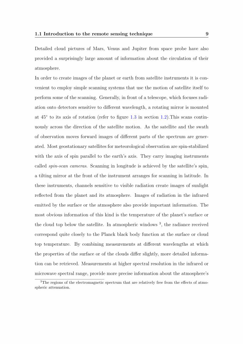
Figure 1.3: Optical schematic of a typical radiometer, showing the elements of asimple filter, a telescope and two spectral channels separated by a dichroic plate. Thisconfiguration include also a scan mirror which can be pointed at the atmosphere, coldspace or a black body at known temperature for calibration purposes.
An instrument which collects radiant energy in a particularly efficient way while
at the same time achieving high spectral resolution is the Michelson Interferometer
(see figure 1.4).
The essential part of the instrument is the beamsplitter, which divides the in-
coming radiation into two beams of nearly equal intensity [9]. After reflection from
the stationary and movable mirrors, the beams recombins at the beamsplitter. The
phase difference between both beams is proportional to their optical path difference,
including a phase shift due to the difference between internal and external reflections
at the beamsplitter. Suppose a collimated beam of monochromatic radiation strikes
the interferometer while the movable mirror is set at the balanced position where
both arms have equal length. In a non-absorbing beamsplitter the phase difference
between internal and external reflection is 180. Consequently, both beams inter-
fere destructively as seen from the detector, the central fringe is dark. At the same
time, the interference is constructive as seen from the entrance port. The incom-
1.2 Remote sensing instruments 13
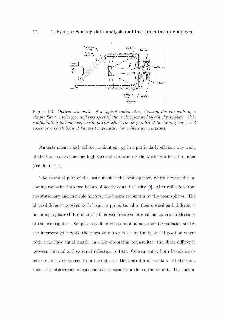
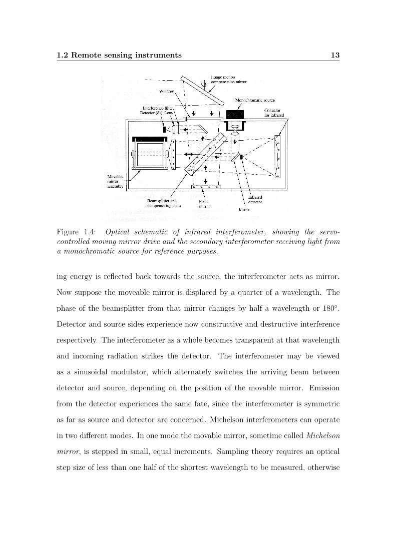
Figure 1.4: Optical schematic of infrared interferometer, showing the servo-controlled moving mirror drive and the secondary interferometer receiving light froma monochromatic source for reference purposes.
ing energy is reflected back towards the source, the interferometer acts as mirror.
Now suppose the moveable mirror is displaced by a quarter of a wavelength. The
phase of the beamsplitter from that mirror changes by half a wavelength or 180.
Detector and source sides experience now constructive and destructive interference
respectively. The interferometer as a whole becomes transparent at that wavelength
and incoming radiation strikes the detector. The interferometer may be viewed
as a sinusoidal modulator, which alternately switches the arriving beam between
detector and source, depending on the position of the movable mirror. Emission
from the detector experiences the same fate, since the interferometer is symmetric
as far as source and detector are concerned. Michelson interferometers can operate
in two different modes. In one mode the movable mirror, sometime called Michelson
mirror, is stepped in small, equal increments. Sampling theory requires an optical
step size of less than one half of the shortest wavelength to be measured, otherwise

14 1. Remote Sensing data analysis and instrumentation employed
aliasing may occur. However, if we know that the signal consists only of a narrow
band of frequencies, sampling may occur at larger intervals without risking confu-
sion due to aliasing. the number of sampling points can be reduced considerably
by this technique. Alternatively, in a method sometime employed in the continuous
mode, the interferometer may be oversampled and the reduction to the minimum
number of necessary data points may be accomplished by numerically filtering after
digitalization. In the stepping mode, the signal is integrated at each rest position
for a certain time, the dwell time. After that, the Michelson mirror moves to the
following position and the next point is recorded. In the continuous mode the mirror
advances at constant speed and the signal is sampled at small, equal intervals. At
one time the misconception existed that this mode is less efficient than the discrete
step mode because the time spent in taking the sample is small in comparison with
the time between sample, but this is not the case. Integration between samples takes
place in the electrical filter used to limit the frequency range before the sampling
process. On the contrary, the stepping mode is slightly less efficient, because the
time spent while moving the mirror between measurement points is loss.
As the whole spectrum is observed all the time, the Michelson Interferometer pos-
sesses what is called the multiplex advantage; observation from many spectral chan-
nels can be made simultaneously.
In the case of planetary atmospheres, the radiation measured by the instrumentation
on board of spacescraft, consists of many spectral line and radiation continuum. To
resolve each single line it’s convenient to use a grating spectrometer. The diffraction
grating is of considerable importance in spectroscopy, due to its ability to separate
(disperse) polychromatic light into its constituent monochromatic components. A
grating consists of a series of equally separated, parallel slits or apertures, the width
1.2 Remote sensing instruments 15
of each being comparable to the wavelength of radiation to be separated. It may be
thought of as a collection of diffracting elements, such as a pattern of transparent
slits in an opaque screen, or a collection of reflecting grooves on a substrate (also
called a blank). The slits may be supported on a material which transmits or reflects
the radiation and the grating is then called a transmission or a reflection grating,
respectively. The fundamental physical characteristic of a diffraction grating is the
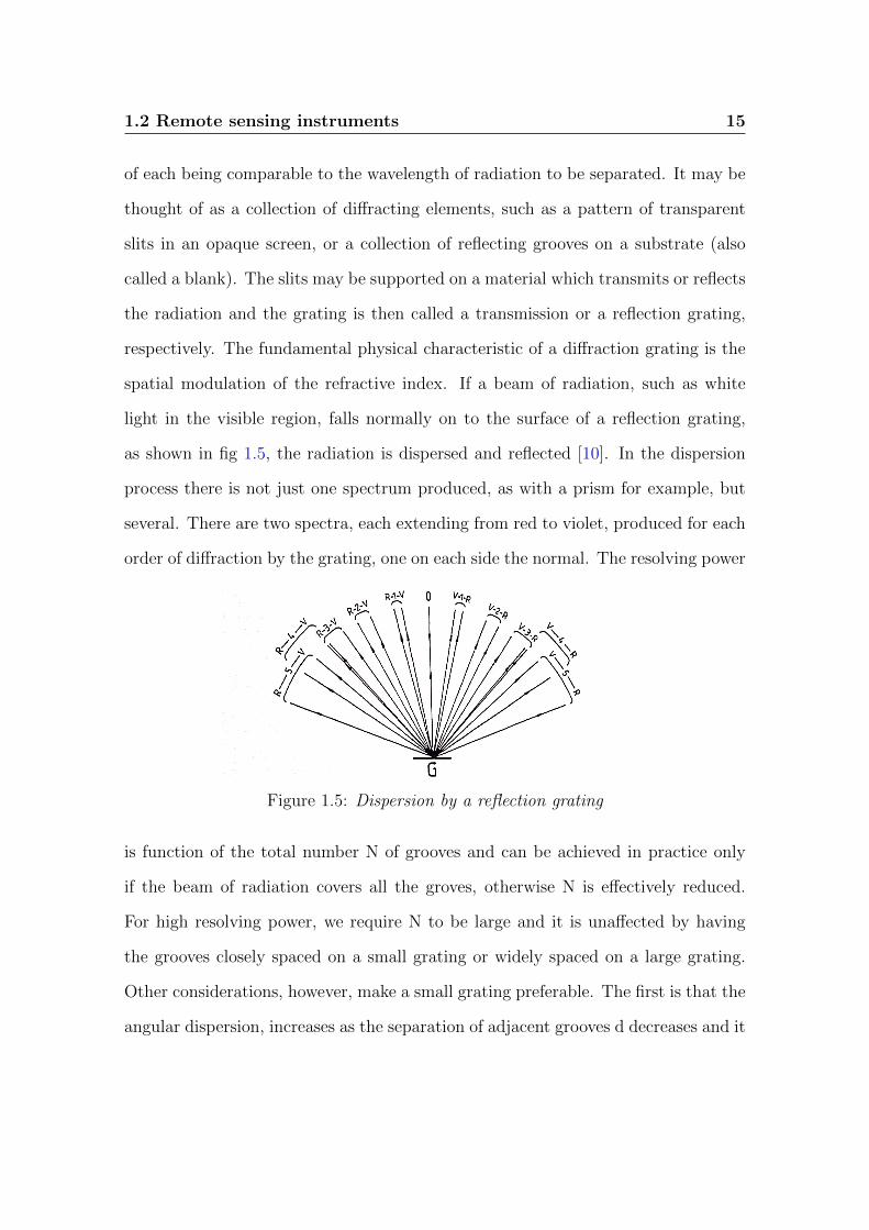
spatial modulation of the refractive index. If a beam of radiation, such as white
light in the visible region, falls normally on to the surface of a reflection grating,
as shown in fig 1.5, the radiation is dispersed and reflected [10]. In the dispersion
process there is not just one spectrum produced, as with a prism for example, but
several. There are two spectra, each extending from red to violet, produced for each
order of diffraction by the grating, one on each side the normal. The resolving power
Figure 1.5: Dispersion by a reflection grating
is function of the total number N of grooves and can be achieved in practice only
if the beam of radiation covers all the groves, otherwise N is effectively reduced.
For high resolving power, we require N to be large and it is unaffected by having
the grooves closely spaced on a small grating or widely spaced on a large grating.
Other considerations, however, make a small grating preferable. The first is that the
angular dispersion, increases as the separation of adjacent grooves d decreases and it

16 1. Remote Sensing data analysis and instrumentation employed
is no good having a grating with high resolving power if the dispersion is so low that
the detector is unable to distinguish wavelengths which the grating has resolved.
The second consideration favouring a small grating is that a large on required large
lens, large mirrors and so on in order to fill it with radiation and this again increases
the size of the instrument.
The possible modes to illuminating a grating and gathering the light reflected from
it, not only in the far infrared but also in the mid and near infrared, visible and
violet regions, are numerous. The most famuose configuration is the Ebert-Fasties
mounting, as shown in figure 1.6. Radiation from the source S enters the spectrom-
eter at the slit S1 which is separeted from the mirror M by its focal lenght f so that
the grating G recevies a parallel beam from M. The grating reflects and desperses
the radiation which is focused by M on to the slit S2 and pass to the detector D. The
required wavenumber range is scanned across S2 by smooth rotation of the grating.
An important property of this configuration is that the aberrations produced by
using the mirror off-axis at the first reflection are cancelled by the aberration on the
second reflection.
Figure 1.6: The Ebert-Fastie mounting of a diffraction grating.
1.3 Radiative transfer processes 17
A sophisticated spectrometer designed to collect images and spectroscopic data
of the Venus’s atmosphere is VIRTIS. The acronym stands for Visible and InfraRed
Thermal Imaging Spectrometer and is an instrument which covers the wavelength
range from 0.3 to 5 µm. In the section 1.4, you can find a detailed description of this
instrument on board of the European Space Agengy (ESA) Venus Express mission
(VEX).
1.3 Radiative transfer processes
Various physical processes modify a radiation field as it propagates through an at-
mosphere. The rate at which the atmosphere emits depends on its composition and
thermal structure, while its absorption and scattering properties are defined by the
pravailing molecular opacity and cloud staructure.
To describe the extinction of a beam of radiation crossing a homogeneous atmo-
spheric layer dl with an incidence angle cos θ, we defined the optical depth. Once
divided for cos θ, this quantity can be interpreted as the average number of inter-
actions with matter of a photon with wavenumber ν crossing the depth dl. The
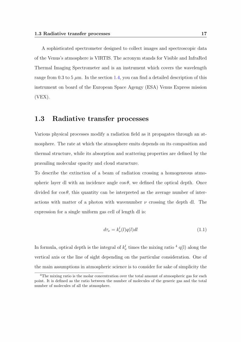
expression for a single uniform gas cell of length dl is:
dτν = klν(l)q(l)dl (1.1)
In formula, optical depth is the integral of klν times the mixing ratio 4 q(l) along the
vertical axis or the line of sight depending on the particular consideration. One of
the main assumptions in atmospheric science is to consider for sake of simplicity the
4The mixing ratio is the molar concentration over the total amount of atmospheric gas for eachpoint. It is defined as the ratio between the number of molecules of the generic gas and the totalnumber of molecules of all the atmosphere.

18 1. Remote Sensing data analysis and instrumentation employed
atmosphere as composed of a finite number of plane and parallel layers each with
uniform temperature and pressure in its interior.
At the radiation crossing between the levels l0 = 0 and l1 = z1 is associated an
optical depth of:
τν =
∫ l1
l0
klν(l)q(l)dl (1.2)
Therefore optical depth is the integral calculated along the line of sight of absorption
coefficient klν multiplied by the mixing ratio q(l). In our case, the optical path is
equal to the length of the gas cell, i.e. 2 cm.
It is now possible to calculate the attenuation of the radiation. Transmittance, along
the line of sight, is simply the exponent of the optical depth:
tν = exp−( τν
cos θ
)(1.3)
In the solar region, we often deal with the total transmittance of the atmosphere
from the space to the surface and back:
tν = exp−[τν
(1
cos θ0
+1
cos θ
)](1.4)
where τν is the total optical depth in the nadir (strictly vertical) direction, θ0 is the
sun zenith angle and θ is the line of sight zenith angle.
For the pourpuse of this work, we consider only the case of the radiative Ttransfer
without scattering, i.e. whene the effect of aerosols is negligible. The Radiative
Transfer Equation is calculated as the integral of the Planck function on transmit-
tance (which depends on altitude) from the bottom level (or a reference altitude) to
the top of the atmosphere, plus an additional term taking into account the surface
1.3 Radiative transfer processes 19
emission.
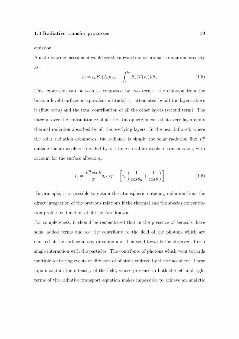
A nadir viewing instrument would see the upward monochromatic radiation intensity
as:
Iν = ενBν(T0)tν,0 +
∫ t0
0
Bν(T (τν))dtν (1.5)
This expression can be seen as composed by two terms: the emission from the
bottom level (surface or equivalent altitude) εν , attenuated by all the layers above
it (first term) and the total contribution of all the other layers (second term). The
integral over the transmittance of all the atmosphere, means that every layer emits
thermal radiation absorbed by all the overlying layers. In the near infrared, where
the solar radiation dominates, the radiance is simply the solar radiation flux F 0ν
outside the atmosphere (divided by π ) times total atmosphere transmission, with
account for the surface albedo aν .
Iν =F 0ν cos θ
πaνexp−
[τν
(1
cos θ0
+1
cos θ
)](1.6)
In principle, it is possible to obtain the atmospheric outgoing radiation from the
direct integration of the previous relations if the thermal and the species concentra-
tion profiles as function of altitude are known.
For completeness, it should be remembered that in the presence of aerosols, have
some added terms due to: the contribute to the field of the photons which are
emitted at the surface in any direction and then send towards the observer after a
single interaction with the particles. The contribute of photons which went towards
multiple scattering events or diffusion of photons emitted by the atmosphere. These
inputs contain the intensity of the field, whose presence in both the left and right
terms of the radiative transport equation makes impossible to achieve an analytic
20 1. Remote Sensing data analysis and instrumentation employed
solution of equation 1.3.
1.4 The Visible and InfraRed Thermal Imaging
Spectrometer
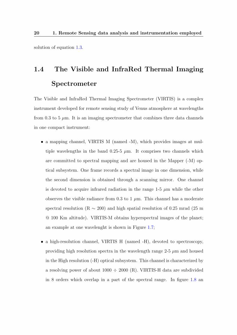
The Visible and InfraRed Thermal Imaging Spectrometer (VIRTIS) is a complex
instrument developed for remote sensing study of Venus atmosphere at wavelengths
from 0.3 to 5 µm. It is an imaging spectrometer that combines three data channels
in one compact instrument:
• a mapping channel, VIRTIS M (named -M), which provides images at mul-
tiple wavelengths in the band 0.25-5 µm. It comprises two channels which
are committed to spectral mapping and are housed in the Mapper (-M) op-
tical subsystem. One frame records a spectral image in one dimension, while
the second dimension is obtained through a scanning mirror. One channel
is devoted to acquire infrared radiation in the range 1-5 µm while the other
observes the visible radiance from 0.3 to 1 µm. This channel has a moderate
spectral resolution (R ∼ 200) and high spatial resolution of 0.25 mrad (25 m
@ 100 Km altitude). VIRTIS-M obtains hyperspectral images of the planet;
an example at one wavelenght is shown in Figure 1.7;
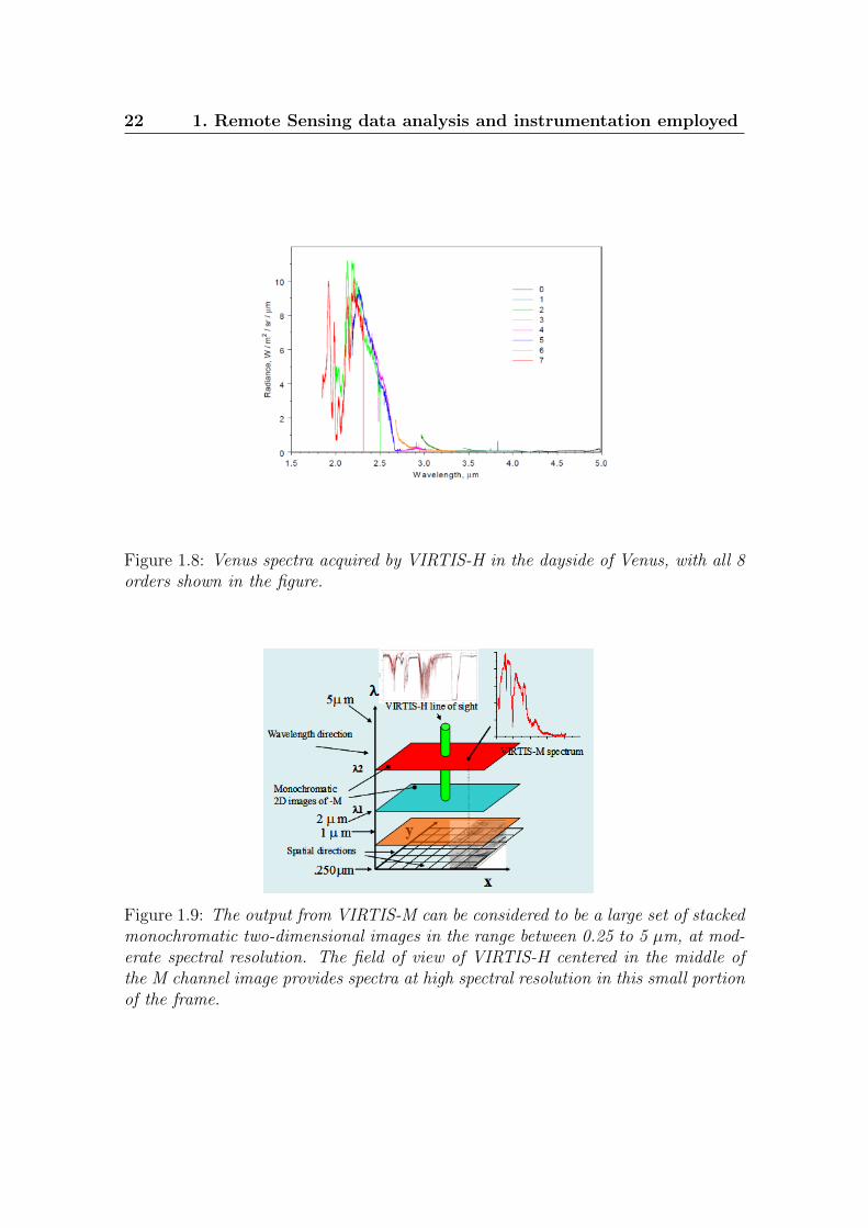
• a high-resolution channel, VIRTIS H (named -H), devoted to spectroscopy,
providing high resolution spectra in the wavelength range 2-5 µm and housed
in the High resolution (-H) optical subsystem. This channel is characterized by
a resolving power of about 1000 ÷ 2000 (R). VIRTIS-H data are subdivided
in 8 orders which overlap in a part of the spectral range. In figure 1.8 an

1.4 The Visible and InfraRed Thermal Imaging Spectrometer 21
example of VIRTIS-H spectrum with all orders is shown. Order 0 starts at 5
micron, till order 7 up to 2 micron. The resolution is higher in the spectral
region at lower wavelengths of each order, but due to some residual stray light
on should infer, case by case, the best order for the specific study.
Figure 1.7: A suggestive image of the Venus polar region acquired by VIRTIS-M @5 µm. We can observe the polar vortex called dipole for its shape.
22 1. Remote Sensing data analysis and instrumentation employed
Figure 1.8: Venus spectra acquired by VIRTIS-H in the dayside of Venus, with all 8orders shown in the figure.
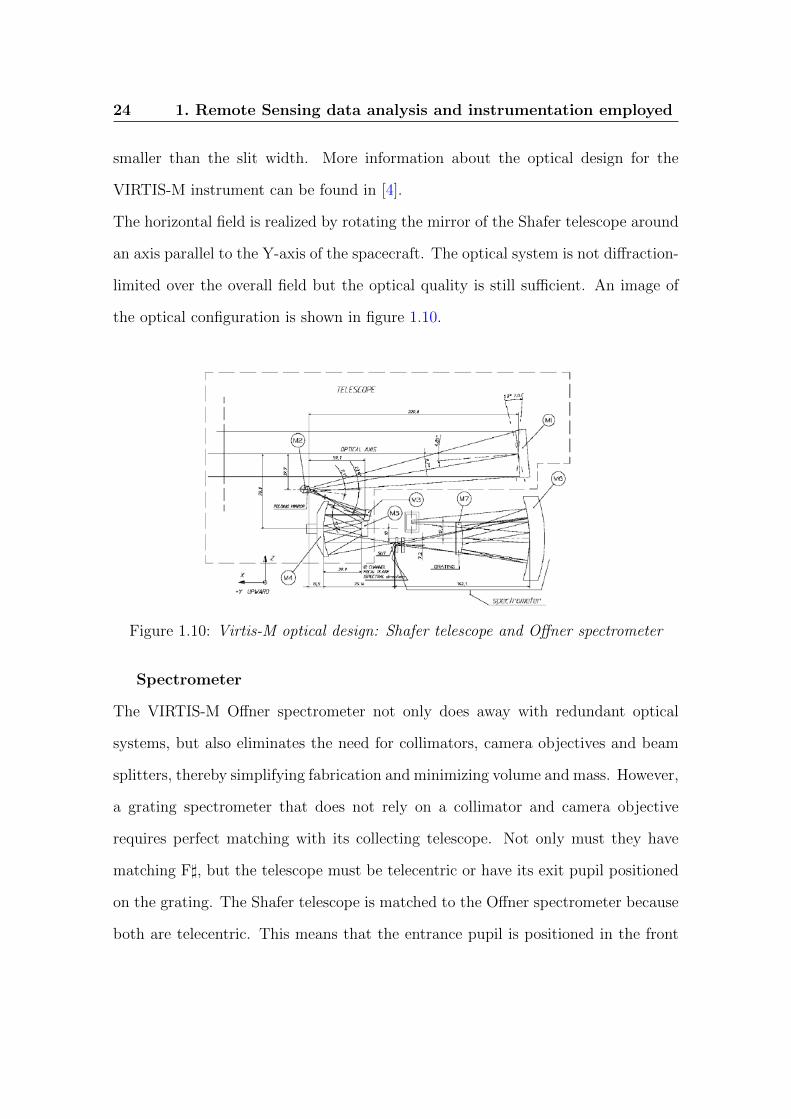
Figure 1.9: The output from VIRTIS-M can be considered to be a large set of stackedmonochromatic two-dimensional images in the range between 0.25 to 5 µm, at mod-erate spectral resolution. The field of view of VIRTIS-H centered in the middle ofthe M channel image provides spectra at high spectral resolution in this small portionof the frame.

1.4 The Visible and InfraRed Thermal Imaging Spectrometer 23
The focal planes, with Charge Coupled Device (CCD) and infrared detectors
achieve high sensitivity for low intensity sources. Due to the high flexibility of
the operational modes of VIRTIS, these performances are ideally adapted for the
study of Venus atmosphere, both on night and day sides. In fact, VIRTIS provides
a 4-dimensional study of Venus atmosphere (2D imaging + spectral dimension +
temporal variations), the spectral variations permitting a sounding at different lev-
els of the atmosphere, from the ground up to the lower thermosphere. The infrared
capability of VIRTIS is especially well fitted to the thermal sounding of the night
side atmosphere which gives a tomography of the atmosphere down to the surface;
information about the clouds can also be retrieved from dayside observations and
in both InfraRed and visible range.
In Figure 1.9 a simple graphic representation of the output data is given.
1.4.1 VIRTIS M
Telescope
The Shafer-type telescope is the combination of an inverted Burch telescope and
an Offner relay. The Offner relay takes the curved, anastigmatic virtual image of the
inverted telescope and makes it flat and real without losing the anastigmatic quality.
Coma optical aberration is eliminated by putting the aperture stop near the center of
curvature of the primary mirror, thus making the telescope monocentric. The result
is a telescope system that relies only on spherical mirrors yet remains diffraction-
limited over an appreciable spectrum and all the vertical field (slit direction). At
±1.8 degrees the spot diameters are less than 6 µm in diameter, which is 7 times
24 1. Remote Sensing data analysis and instrumentation employed
smaller than the slit width. More information about the optical design for the
VIRTIS-M instrument can be found in [4].
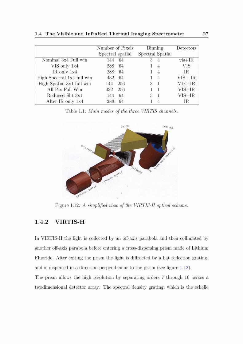
The horizontal field is realized by rotating the mirror of the Shafer telescope around
an axis parallel to the Y-axis of the spacecraft. The optical system is not diffraction-
limited over the overall field but the optical quality is still sufficient. An image of
the optical configuration is shown in figure 1.10.
Figure 1.10: Virtis-M optical design: Shafer telescope and Offner spectrometer
Spectrometer
The VIRTIS-M Offner spectrometer not only does away with redundant optical
systems, but also eliminates the need for collimators, camera objectives and beam
splitters, thereby simplifying fabrication and minimizing volume and mass. However,
a grating spectrometer that does not rely on a collimator and camera objective
requires perfect matching with its collecting telescope. Not only must they have
matching F], but the telescope must be telecentric or have its exit pupil positioned
on the grating. The Shafer telescope is matched to the Offner spectrometer because
both are telecentric. This means that the entrance pupil is positioned in the front

1.4 The Visible and InfraRed Thermal Imaging Spectrometer 25
focal length of the optical system 750 mm in front of the primary mirror. The
VIRTIS-M spectrometer grating does away with the beam splitter by realising two
different groove densities [11] on a single substrate. An image is shown in figure
1.11. Since the pupil optics conjugate is on the grating, the same spectral beam
Figure 1.11: The VIRTIS-M grating used for the development model. The two innerregions are for the visible range, the external one is for IR. The dispersion axis isroughly along the ruler. The surface geometry is convex.
splitting is performed for each Field Of View (FOV) angle. The grating profiles
are holographically recorded into a photoresist coating and then etched with an ion
beam. Using various masks, the grating surface can be separated into different zones
with different groove densities and different groove depths.
The visible Focal Plane Array (FPA) is based on the Thomson-CSF TH7896
CCD detector. It uses a buried channel design and two poly-silicon N-MOS technol-
ogy to achieve good electro-optical performance. It includes a multi-pinned phase
boron implant to operate fully inverted and to reduce substantially the surface dark
current, residual images after strong exposure and other effects due to ionizing ra-
diation. In order to generate the required information (to meet the instantaneous
FOV of 250 µrad and to have the same pixel size in the IR and visible detectors), 2 x

26 1. Remote Sensing data analysis and instrumentation employed
2 binning is implemented at the detector level. This approach achieves the required
pixel size with a less expensive solution; a 38 µm pixel size is feasible but would
require a custom design. The detector is also equipped with two ordering filters
with a boundary at band 215 (680 nm) in order to attenuate the higher orders of
the visible grating region.
The IR detectors used in VIRTIS-H and VIRTIS-M are based on a 2-D array
of IR-sensitive photovoltaic mercury-cadmium-tellurium (HgCdTe). These devices
have the potential to operate at a higher temperature than the more established
indium antimonide (InSb) detectors owing to dark current reduction by a factor
of 10 or more. The array is formed through hybridisation of mercury-cadmium-
telluride (MCT) material with dedicated Si CMOS. The device is a MCT-Si hybrid
array of 270(w) x 436(h) 38 µm MCT photodiodes with line and column spacing
of 38 µm between diode centres, a spectral wavelength range from 0.95 µm up to 5
µm and an operating temperature of 80K. The detector is packaged into a housing
which includes an optical window and provides mechanical, thermal and electrical
interfaces for its integration on the VIRTIS-H and -M FPAs. The VIRTIS-M filter
window is used to stop the superimposition of higher diffraction orders from the
grating and also to eliminate/reduce the background thermal radiation due to the
temperature of the instrument housing.
The possible modes for VIRTIS-M are summarized in Table 1.1. The overall
data rate and volume depend essentially on the selected modes for -M because -H
does not much affect the rate (unless special testing modes are used, involving the
transfer of the full frame).
1.4 The Visible and InfraRed Thermal Imaging Spectrometer 27
Number of Pixels Binning DetectorsSpectral spatial Spectral Spatial
Nominal 3x4 Full win 144 64 3 4 vis+IRVIS only 1x4 288 64 1 4 VISIR only 1x4 288 64 1 4 IR
High Spectral 1x4 full win 432 64 1 4 VIS+ IRHigh Spatial 3x1 full win 144 256 3 1 VIE+IR
All Pix Full Win 432 256 1 1 VIS+IRReduced Slit 3x1 144 64 3 1 VIS+IRAlter IR only 1x4 288 64 1 4 IR
Table 1.1: Main modes of the three VIRTIS channels.
Figure 1.12: A simplified view of the VIRTIS-H optical scheme.
1.4.2 VIRTIS-H
In VIRTIS-H the light is collected by an off-axis parabola and then collimated by
another off-axis parabola before entering a cross-dispersing prism made of Lithium
Fluoride. After exiting the prism the light is diffracted by a flat reflection grating,
and is dispersed in a direction perpendicular to the prism (see figure 1.12).
The prism allows the high resolution by separating orders 7 through 16 across a
twodimensional detector array. The spectral density grating, which is the echelle

28 1. Remote Sensing data analysis and instrumentation employed
element of the spectrometer, to achieve very high spec resolution, λ ∆λ, varies in
each order between 1200 and 3500. Since -H is not an imaging channel, it is only
required to achieve good optical performance at the zero field position. The focal
length of the objective is set by the required IFOV and the number of pixels allowed
for summing. While the telescope is f/1.6, the objective is f/1.67 and requires five
pixels to be summed in the spatial direction to achieve a 1 mrad2 IFOV (5 x .45
mrad x .45 mrad). VIRTIS-H uses the same IR detector as VIRTIS-M however, due
to the different design of the two channels, the detector is used rather differently.
VIRTIS-H is a high resolution spectrometer and does not perform imaging; the H-IR
detector is used to acquire spectra spread over its surface, thus only a portion of the
pixels contains useful scientific data. The 8 spectral orders are spread over the entire
surface matrix. In each spectral order the spectrum covers 432x5 pixels (where 5
pixels represent the image of the slit size when imaged on the detector). Thus overall
only 15% of the 438x270 pixels matrix surface is used. To reduce the overall data
rate and volume, H uses the so called Pixel Map which gives the exact location of the
spectra over the H-IR detector. The ME calculates the location of the pixels to be
downloaded and passes it to PEM-H (Proximity Electronics Module-H) which then
downloads them accordingly. The downloaded data are the H-SPECTRUM, a set of
432x8x5. One H-Spectrum can be defined as a composition of the 8 orders imaged on
the H-IR detector, the H-Spectrum is extracted from the two-dimensional detector
by using a map of the lighted pixels based on 8 spectral orders of 432 elements and
a width of 5 pixels for each order. The 5 pixels are reduced to 1 pixel by averaging.
As H has no spatial resolution the 5 pixels are averaged together, thus the final end-
product in the H-Nominal acquisition mode is a 3456 (or 432x8) pixels spectrum
representing the full spectral range of the instrument from 1.88 through 5.03 µm.

1.4 The Visible and InfraRed Thermal Imaging Spectrometer 29
The main characteristics of the two instruments are summarized in table 1.2.

30 1. Remote Sensing data analysis and instrumentation employed
VIRTIS-M VIRTIS-M VIRTIS-H(Visible) (InfraRed)
Spectral range (µm) 0.3-1.1 1.0 - 5.1 Or0 4.01206-4.98496Or1 3.44270-4.28568Or2 3.01190-3.75586Or3 2.67698-3.33965Or4 2.40859-3.00570Or5 2.18903-2.73220Or6 2.00565-2.50468Or7 1.85100-2.31194
Spectral resolution 100-380 70-360 1300-3000λ/ ∆λ
Spectral Sampling 1.89 9.44 0.6(nm)
Field of View 63.6 (slit) x 64.2 (scan) 0.567 x 1.73(mrad x mrad)
Spatial Resolution 250 (slit) x 250(scan)(µrad)
Full FOV high resolution 256 x 256Image size (pixels)Noise equivalent 1.4x10⁻¹ 1.2x10⁻⁴ 1.2x10⁻⁴
Spectral radiance(Wm−2sr−1µm−1)
Telescope Shafer Telescope Shafer Telescope Off-axisparabolic mirror
pupil diameter 47.5 32(mm)
Imaging F] 5.6 3.2 2.04Etendue 4.6x10⁻¹¹ 7.5x10⁻¹¹ 0.8x10−09
(m2sr)Slit dimension 0.038x9.53 0.029 x 0.089
(mm)Spectrometer Offner Relay Offner Relay Echelle spectrometer
Detectors Thomson TH7896 CCD HgCdTe HgCdTeSensitivity area format 508 x 1024 270 x 436 270 x436
Pixel pitch (mm) 19 38 38Operating Temperature (K) 150-190 65-90 65-90
Spectral range (µm) 0.25-1.05 0.95-5.0 0.95-5.0Mean dark current < e/s <2 fA @ 90K < 2 fA @ 90 K
Table 1.2: Main characteristics of the three VIRTIS channels.

1.5 Scientific goals of VIRTIS 31
1.5 Scientific goals of VIRTIS
VIRTIS is able to produce day and nightside IR and visible spectra. The whole at-
mosphere is being observed from the mesospheric levels down to the surface ([12]),
and the surface itself is accessible to VIRTIS IR observations on the nightside. The
main topics for VIRTIS science observations are [13]:
F study of the lower atmosphere composition below the clouds and its variations
(CO, OCS, SO2, H2O) from nightside observations [14]. The 2.3 µm window gives
access to accurate measurement of minor species. At shorter wavelengths, H2O is
measurable with VIRTIS-M for mapping H2O variations, as done by NIMS/Galileo
[15]. From these observations, correlation with volcanic or meteorological activity is
being sought [16](some signatures of volcanic outgassing are related to minor-species
variations, in particular for sulphur compounds).
F study of the cloud structure, composition and scattering properties (dayside and
nightside)[17]. The different geometries of cloud reflections along with the spectral
range of VIRTIS will constrain the cloud structure. The average structure is known
from previous missions, but the temporal and spatial variabilities are less well docu-
mented. VIRTIS can sound the different layers and measure their optical thickness
in the IR, and measure the upper layer on the dayside.
F cloud tracking in the UV [18](∼ 70 km altitude, dayside) and IR (45 km altitude,
nightside). The correlation of UV and IR observations at different times, along with
the 4-day cloud rotation period, gives access to the vertical variation of the wind
field up to 70 km altitude.
F measurements of the temperature field with subsequent determination of the
zonal wind in the altitude range 65-100 km (nightside)[19]. The 4-5 µm range is

32 1. Remote Sensing data analysis and instrumentation employed
sensitive to thermal structure, which can be retrieved (on the nightside) and com-
pared with models [20]. Such retrieval gives access to the vertical wind variations
through cyclostrophic approximation.
F lightning search (nightside). Although tentative (there is no reliable information
on the frequency of lightning on Venus), observations of transient lightning illu-
mination are of high scientific interest, and is an ’open search’ option for VIRTIS
observations.
F mesospheric sounding. Understanding the transition region between troposphere
and thermosphere: - non-local thermodynamic equilibrium (non-LTE) O2 emission
(night/dayside) at 1.27 µm (95-110 km; [15]). As observed from the ground and
NIMS/Galileo, these emissions have spatial and temporal variabilities, which make
them of high interest for accurate spatial mapping by VIRTIS.
F CO2 fluorescence (dayside). Non-LTE emissions at 4.3 µm ( >80 km; [21] on limb
scans by Galileo provide important information on the physics of the upper atmo-
sphere through the collisional/radiative equilibrium sounded through the CO2 band.
F limb observations (CO, CO2)[22]: atmospheric vertical structure (>60 km) (day/night-
side).
F search for variations related to surface/atmosphere interaction, dynamics, me-
teorology and volcanism. Global observation or partial observations at a regional
scale on a temporal scale of one Venusian day is allowing the search for correlations
between different physical processes.
F temperature mapping of the surface and searching for hot spots related to vol-
canic activity. NIMS/Galileo observations of Io showed that lava lakes are easily
detected on a planet by imaging spectroscopy. Even if the atmosphere of Venus pre-
cludes the clear detection of free lava, a temperature anomaly could be a signature

1.5 Scientific goals of VIRTIS 33
of some volcanic activity. This has never been attempted with the spatial/temporal
performance of an instrument like VIRTIS.
F search for seismic waves from the propagation of acoustic waves amplified in the
mesosphere by looking for high-altitude variations of pressure/ temperature in the
CO2 4.3 µm band [23]. Although clearly a challenge, it is one of the tentative sci-
ence objectives that would be of primary scientific importance if detected. Gravity
waves also have signatures in the IR mesospheric emissions accessible to VIRTIS.
Very little is known about wave activity in the upper atmosphere of Venus.

Chapter 2
Planetary atmospheres and
notions of spectroscopy
In the previous chapter the remote sensing techniques and the instrumentation em-
ployed have been described. A lot of importance has been given to the VIRTIS, the
complex spectrometer devoted to study of the Venus atmosphere. In this chapter,
we’ll give a brief description of the planet considered Earth’s twin of size and mass.
Besides, in the second part of the chapter we will introduce notions of spectroscopy,
a powerful tools of investigation in the field of planetary science. Infrared spec-
troscopy and present-day high resolution spectrometers have demonstrated to be
one of the most powerful remote sensing tools in the context of planetary obser-
vation, for atmospheric as well as for surface studies: they give together a remote
access to most of the important information carried by the radiation which directly
interacted with the planet.

36 2. Planetary atmospheres and notion of spectroscopy
2.1 Venus
Venus, the ”Morning Star”, is Earth’s closest neighbor, the second planet from the
Sun and belongs to the family of terrestrial planets, alongside Earth, Mars and
Mercury [12]. Its small rotation axis obliquity and orbital eccentricity ensures that
no seasons affect its rocky surface where the temperatures rise close to 500C with
a pressure 90 times the Earth’s one. Known since ancient times due to its brilliant
color, brightness and unusual appearances in the sky, Venus is a planet similar to
the Earth in mass and radius but has no moon and no magnetic field shielding it
from cosmic rays and solar winds. Venus’ obliquity is only 2.6, compared to 24 of
the Earth and Mars and orbits in the prograde direction about the Sun in a nearly
circular orbit every 224.7 earth days. Its rotation relative to the stars, the sidereal
motion, is retrograde every 243.01 earth days. If the Sun could be seen from the
surface of the planet, it would make roughly one complete circuit of the Venusian
sky in half a Venus year. Hence, the length of the Venus day, also known as the
solar day, is 116.75 Earth days. Since Venus is closer to the Sun than the Earth,
the planet shows phases when viewed with a telescope: sometimes it appears as a
crescent, others half-illuminated and others nearly full. Galileo Galilei’s (1564-1642)
astounding observation of this phenomenon in late 1610 was the first 19 irrevocable
piece of important evidence in favor of Copernicus’s heliocentric theory of the solar
system. As an inferior planet Venus revolves around the Sun faster than the Earth;
and as the two planets are moving in the same direction around the Sun, Venus
appears for a few months in the early morning, some hours before sunrise, then
disappears only to be seen as a bright moon-like object emerging after sunset for
a further few months before disappearing again. The main orbital and solid body
2.1 Venus 37
characteristics of Venus and Earth are given in table 2.1 for easy comparison, while
in table 2.2 the Venusian observational parameters are presented.
Venus was explored by a fleet of American and Soviet spacecraft starting with
Mariner 2 in 1962, the first successful spacecraft to fly-by Venus, up to the Magellan
orbiter in 1990, which produced global detailed maps of Venus’ surface using radar
mapping, altimetry and radiometry techniques with a resolution of about 100 m.
In between, more than twenty missions have explored Venus, including the Soviet
Venera 7 in 1970 which was the first spacecraft to land on another planet, Venera 9 in
1975 which returned the first photographs of the surface and the American Pioneer
Venus Orbiter in 1978 which carried several atmospheric environment experiments
and four entry probes. Magellan’s observations further revealed that the surface
of Venus is mostly covered by volcanic materials. Volcanic surface features, such
as vast lava plains, fields of small lava domes and large volcanoes are common. A
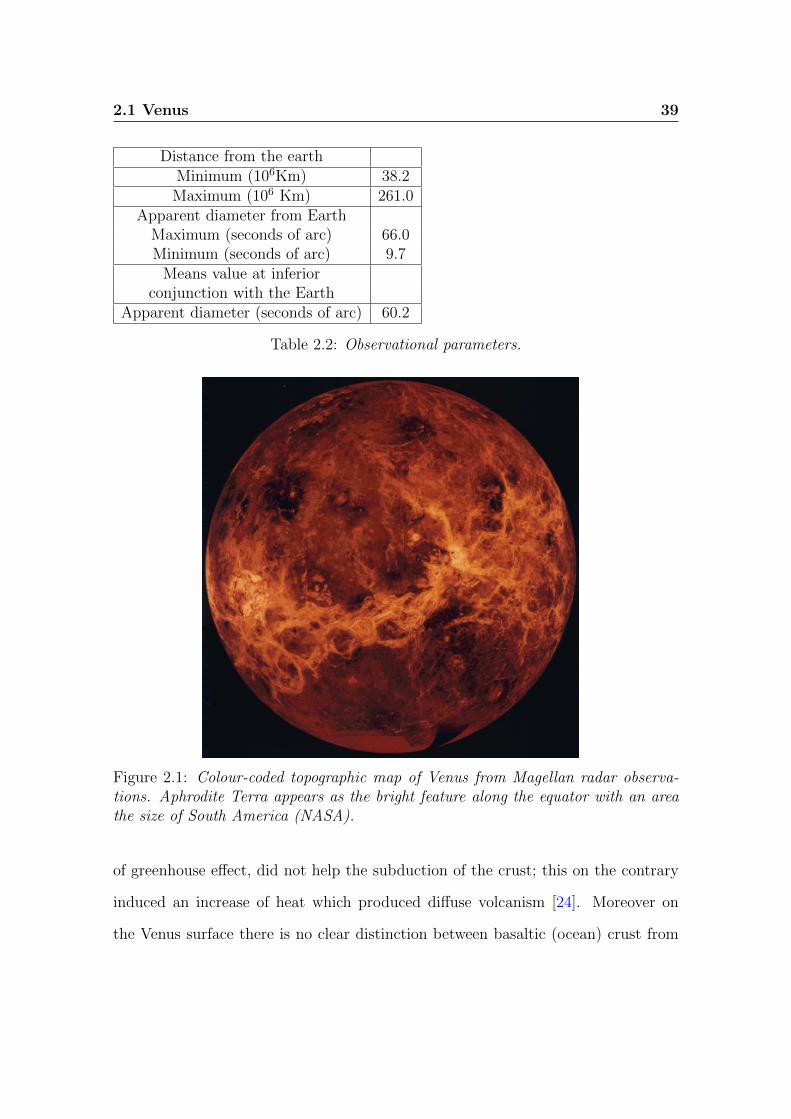
color-coded composite of these observations is shown in figure 2.1.
Venus has two major continents, Aphrodite Terra and Ishtar Terra, which occupy
only a few percent of the total surface area. Aphrodite Terra, seen figure 2.1, is a
long, narrow area which stretches over 150 in longitude and contains a few peaks
higher than 8 km. The planetary elevation is calculated over the mean radius of the
planet, 6050 km. Ishtar Terra contains the highest elevation region, Maxwell Montes,
around 65 N which rises to altitudes of 10.5 km above mean planetary radius. The
remainder of the surface of Venus is covered mostly by volcanic materials .
Although Venus has a dense atmosphere, the surface shows no evidence of substantial
wind erosion, and there has been only slight evidence of limited wind transport of
dust. On Venus we cannot find evidence of plate tectonics (trenches, ridges), as the
absence of water in the surface, which evaporated and went lost with the increase

38 2. Planetary atmospheres and notion of spectroscopy
VENUS EARTH VENUS/ EARTHBulkparametersMass (1024 Kg) 4.8685 5.9736 0.815
Volume (1010 km3) 92.843 108.321 0.857Equatorial radius (km) 6051.8 6378.1 0.949
Polar Radius (Km) 6051.8 6356.8 0.952Volumetric mean radius (Km) 6051.8 6371.0 0.950Ellipticity (polar flattening) 0.000 0.00335 0.0
Mean density (Kg/m3) 5243 5515 0.951Surface gravity at equator (m/s2) 8.87 9.80 0.905
Escape velocity (km/s) 10.36 11.19 0.926Bond albedo 0.76 0.30 2.53
Visual geometric albedo 0.65 0.367 1.77Solar irradiance (W/m2) 2613.9 1367.6 1.911Equivalent BlackBody 231.7 254.3 0.911
Temperature (K)Topographic range (Km) 15 20 0.750
OrbitalparametersSemi major axis (106 Km) 108.21 149.60 0.723Sideral orbit period (days) 224.701 365.256 0.615
Tropical orbit period (days) 224.695 365.242 0.615Perihelion (106 Km) 107.48 147.09 0.731Aphelion (106 Km) 108.94 152.10 0.716
Synodicnvelocity (days) 583.92 - -Mean orbital velocity (km/s) 35.02 29.78 1.176Max. orbital velocity (km/s) 35.26 30.29 1.164Min orbital velocity ( km/s) 34.79 29.29 1.188
Orbit inclination (deg) 3.39 0.00 -Orbit eccentricity 0.0067 0.0167 0.401
Sideral rotation period (h) 5832 523.9345 243.686Length pf day (h) 2802.0 24.0000 116.750Obliquity (deg) 177.36 23.45 0.113
Table 2.1: Venus/ Earth comparison (after Williams,2005).
2.1 Venus 39
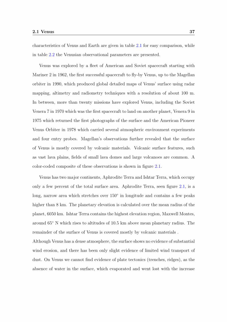
Distance from the earthMinimum (106Km) 38.2Maximum (106 Km) 261.0
Apparent diameter from EarthMaximum (seconds of arc) 66.0Minimum (seconds of arc) 9.7
Means value at inferiorconjunction with the Earth
Apparent diameter (seconds of arc) 60.2
Table 2.2: Observational parameters.
Figure 2.1: Colour-coded topographic map of Venus from Magellan radar observa-tions. Aphrodite Terra appears as the bright feature along the equator with an areathe size of South America (NASA).
of greenhouse effect, did not help the subduction of the crust; this on the contrary
induced an increase of heat which produced diffuse volcanism [24]. Moreover on
the Venus surface there is no clear distinction between basaltic (ocean) crust from
40 2. Planetary atmospheres and notion of spectroscopy
continental granitic crations, as observed on our planet. The absence of craters on
Venus is an indication of a young surface, which is dated no more than 1 Gy.
2.1.1 Venus’s atmosphere
The atmospheric composition of Venus is dominated by CO2 (96.5%), with a few
percent of N2 (3.5%) and a number of trace gases like H20, CO and SO2 in the
parts per million scale [25]. This composition resembles the atmosphere of Mars
which is also made of C02 and N2 and is instead very different from the terrestrial
atmosphere where N2 and O2 play the leading part. The high surface temperature of
Venus (750 K) is significantly above its effective temperature, that is, the equilibrium
temperature expected from its heliocentric distance. Indeed, the surface and the
lower atmosphere of Venus have been heated by a runaway greenhouse effect, mostly
to be ascribed to the large amounts of gaseous CO2 and H2O which were most likely
present in the primordial atmosphere and, in lesser part, to its cloud coverage.Venus
is covered by a thick cloud deck of sulfuric acid H2SO4, at an altitude of 40-70 km,
which prevents the visible observation of the surface. The atmosphere of Venus may
be divided into three natural regions, a troposphere (surface to 60 km), a mesosphere
(60 to 90 km) and a thermosphere (above 90 km). On Earth we find a troposphere
(surface to 12 km), a stratosphere (12 to 45 km), mesosphere (45 to 85 km) and,
as on Venus, a thermosphere (above 85 km). A scheme of the Venus’ atmosphere
composition is shown in the figure 2.2
Vertical profiles of temperatures on Venus and Earth as a function of pressure
at 30 latitude, as measured by the Pioneer Venus OIR and Nimbus 7 spacecraft
respectively, are presented in figure 2.3 on the left. Throughout the troposphere
and mesosphere the temperature decreases with height, from around 740 K to 100

2.1 Venus 41
Figure 2.2: The structure of Venus’s atmosphere showing the main cloud layer andalso how temperature (blu curve) varied with height.
K on Venus and from 280 K to 210 K on Earth. No temperature inversions can be
seen since UV absorbing ozone that cause the Earth’s stratosphere do not exist in
the Venus’ CO2 dominated atmosphere. On Venus’ dayside the temperature above
85-90 km rises to an exospheric value of around 300 K due to solar EUV absorption
and therefore behaves like the thermosphere on Earth, where temperatures rise from
∼ 180 K to ∼ 1000 K. The nightside upper atmosphere on Venus differs from that
on Earth because Venus’ slow rotation period causes solar heating to be absent for
far too long to maintain the high temperatures found on the dayside. Night side
temperatures on Venus’ thermosphere above 85-90 km in fact do not rise above 100
K, justifying the name of ”cryosphere” (”sphere of cold” in Greek). The Venus
temperature structure above the clouds and the thermosphere/cryosphere region is

42 2. Planetary atmospheres and notion of spectroscopy
shown in Figure 2.3 on the right, as observed by three Pioneer probes and Venera
11 and 12.
Figure 2.3: Vertical profile of pressure vs temperature at 30 of latitude North, asmeasured on Venus by PV OIR and on Earth by Nimbus 7 (on left) [26]. Temper-atures above the main cloud regions derived from the Pioneer probes and Venera 11and 12 (on right) [27].
Due to its slow rotation rate and its obliquity, the troposphere of Venus is almost
isothermal in equatorial and middle latitudes. Near the poles of Venus, starting at
60 N, a long-lived dramatic instability occurs, known as the ”polar collar” (or cold
collar), which takes the form of a ribbon of very cold air about 10 km deep and
1000 km in radius, centered on the pole and situated at about 64 km of altitude.
Inside the polar collar temperatures are about 40 K cooler than outside the feature.
Poleward of the inner region of the collar lies at about 65 km the ”polar dipole”, a
feature consisting of two well-defined warm regions circulating rapidly around the
pole with a period of 2.7 days.
2.2 Notions of molecular spectroscopy 43
2.2 Notions of molecular spectroscopy
Spectroscopy is an extremely powerful tool in the study of atoms and molecules.
It is well known that when an electromagnetic radiation falls on a gaseous, liquid
or solid material, which may be atomic or molecular in nature, the radiation may
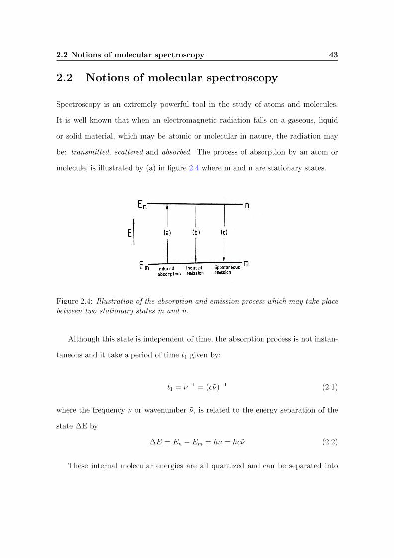
be: transmitted, scattered and absorbed. The process of absorption by an atom or
molecule, is illustrated by (a) in figure 2.4 where m and n are stationary states.
Figure 2.4: Illustration of the absorption and emission process which may take placebetween two stationary states m and n.
Although this state is independent of time, the absorption process is not instan-
taneous and it take a period of time t1 given by:
t1 = ν−1 = (cν)−1 (2.1)
where the frequency ν or wavenumber ν, is related to the energy separation of the
state ∆E by
∆E = En − Em = hν = hcν (2.2)
These internal molecular energies are all quantized and can be separated into
44 2. Planetary atmospheres and notion of spectroscopy
electronic, vibrational and rotational. The first type of energy is typically associ-
ated with the absorption or the emission in the visible part of the electromagnetic
spectrum, the vibrational and rotational are typical of the infrared and microwave
regions, respectively. A molecule consisting of two (or more) nuclei is held together
by valence binding forces of electrons and balanced by internal repulsion forces. The
molecule is in ground state when the outer electronic configuration is in equilibrium
and has potential energy in electronic form when the configuration is unstable due to
acquisition of energy either via absorption or collision. Since the internuclear spac-
ing is large compared to the diameters of the nuclei, which act as point masses, the
molecule possesses moments of inertia about certain axes and can therefore rotate
about them. Small changes in energy levels can produce changes in kinetic energy
of rotation and thus angular velocity of rotation. The valence bond holding the nu-
clei together is not rigid, thus it can be stretched and compressed slightly, creating
changes in intermolecular distance. This elastic bond allows the nuclei to vibrate
about their equilibrium positions; however transitions between vibrational energy
levels require much more energy than those of rotation. Even more energy is needed
for the energy change associated with electronic arrangement. However, vibration
and rotation do not occur separately in nature and observed spectra show both
types of transitions simultaneously in their line structure. The vibration-rotation
combination gives rise to a rotational line structure around each vibrational line.
Quantum mechanics explains the quantized energy states available to an electron
in orbit about a nucleus. Additional consideration of elliptical orbits, relativistic
effects, and magnetic spin orbit interaction was needed to explain the observed
emission spectra in more detail, including the line structure observed. Explanation
of molecular emission lines is still more complicated. Gaseous emission spectra are

2.2 Notions of molecular spectroscopy 45
found to have atomic spectral lines with many additional molecular emission lines
superimposed. The spectra structure is due to the state of the matter and three
major types of molecular excitation are observed:
• line spectra: is a discrete sequence of separated spectral lines at different
frequencies and represents the electronic excitation when the orbital states of
the electrons change in the individual atoms.
• band spectra: is when the lines are condensed in a specific region of frequencies,
forming bands separated each other. It represents the vibrational excitation
when the individual atoms vibrate with respect to the combined molecular
center of mass.
• continuous spectra: is many frequencies in a relatively wide spectral region.
The rotational excitation when the molecule rotates about the center of mass.
2.2.1 Line shape
If a spectrometer was infinitely perfect, the absorption process of a photon by an
atom would show an infinitely narrow feature, a zero width line centered at only one
absolute frequency. For the real instruments, a line is not monochromatic and always
appears spread over a finite wavenumber range with a definite and reproducible line
shape [10]. The instrumentation used for observing a spectrum in fact, is itself one of
the major limiting factor in the observed line shape. But not the only factor. There
are several factors, other than instrumental ones, which contribute to the observed
line shapes. Different physical processes are involved in the absorption and emission
of radiation by atoms or molecules, all contributing to the lines spread. The most
important are the natural line broadening, related to quantum effects, the pressure

46 2. Planetary atmospheres and notion of spectroscopy
broadening and doppler broadening, more related to the physical state of the gas. The
main parameters identyfying a line are the central frequency ν0 where the absorption
or emission occurs, the line intensity S and the shape or profile.
Natural line broadening
According to Heisenberg’s Uncertainty Principle, the Natural line broadening arises
from the finite lifetime ∆t of spontaneous decay transitions. It is a phenomenon
of quantum mechanical nature and implies that the energy levels are not precisely
defined but have spread of values ∆E. This indetermination is reflected to the times
and the frequencies through the famous relation:
∆E∆t = ~ (2.3)
where ~= h/2π with h Planck’s constant.
Being ∆t ∝ (2π∆ν)−1, to each transition is associated a range of frequencies with a
certain probability of interacting with the molecule. The line broadening due to the
natural line width is small relative to most other contributions but is contributed to
in an identical way by each atom or molecule and so is an example of homogeneous
broadening. The natural line broadening is much larger at visible and ultraviolet
wavelengths than at infrared wavelengths and is usually much smaller than the
broadening seen in planetary spectra. The broadening of lines due to the loss of
energy in emission (natural broadening) is practically negligible as compared with
that caused by collisions and the Doppler effect.
Pressure (or Collision) broadening
The second reason of the line width is due to the inevitable interactions between
atoms or molecules. This broadening arises from the fact that collisions between
2.2 Notions of molecular spectroscopy 47
molecules, during a spontaneous state transition, diminish the natural lifetime of
the transition ∆t to the mean time between collisions. If τ is the mean time between
collisions in a gaseous sample and each collision results in a transition between two
different states there is a line broadening ∆ν, coming from:
∆ν = (2πτ)−1 (2.4)
The relation between pressure and line shape was obtained by Lorentz and has
become known as the Lorentzian line shape:
ΦL(ν − ν0) =αL/π
(ν − ν0)2 + α2l
(2.5)
where αL is the Half Width at Half Maximum (HWHM) that, if we use the kinetic
gases theory, is equal to:
αL = αL0p
p0
√T0T (2.6)
where p0 = 1000 mb, T0 = 273K and αL0 is the HWHM value at temperature and
pressure standard conditions. In predicting the line shape due to collisions, Lorentz
assumed that, on collision, the oscillation in the atom or molecule is halted and, after
collision, starts again with a phase completely unrelated to that before collision.
Because αL is proportional to the pressure and being the expression normalized,
for high values of pressure, the contribution of the wings of the function become
important. We mention other two important aspects of the HWHM: αself and αair.
The first one is due to the effect of the pressure of a molecule by all the other
molecules of the same specie, the second one is due to all the other molecules in the
gas. If a specie is only in trace in the atmosphere, the first one is often negligible.

48 2. Planetary atmospheres and notion of spectroscopy
Doppler broadening
It’s well known that the relative motion between an observer and an emitting source
produces the Doppler effect. In a similar way the frequency of the radiation absorbed
during a transition in an atom or molecule differs according to the direction of motion
relative to the source of radiation. The shape of the Doppler line is given by:
ΦD =1√παD
exp−(
(ν − ν0)2
α2D
)(2.7)
with
αD =v0ν0
cν0 =
√2kbT
m(2.8)
where ν0 is the frequency of the photon, v0 is the velocity obtained from the Maxwell
distribution and m is the mass. If for the pressure broadening the pressure is re-
sponsible for the line width, in this case is the temperature. Being αD proportional
to the temperature in fact, heavy molecules give low broadening and vice versa.
In most gas phase spectroscopy, line broadening is due to Doppler (inhomogeneous)
and pressure (homogeneous) broadening, but only a low frequencies is difficult to
reduce pressure broadening to such an extent that Doppler dominates. For example,
in microwave and millimeter wave spectroscopy a typical HWHM intensity is 1-10
KHz due to pressure broadening at pressure of only few bar compared to about
10 KHz due to Doppler. Under these conditions of comparable to inhomogeneous
and homogeneous line broadening, the line shape is a combination of Gaussian and
Lorentzian and is called a Voigt profile.
Voigt line shape
The composite line profile, which must now include the effects of both, is obtained
from the convolution of the two profiles. The Voigt line shape approaches the Lorentz

2.2 Notions of molecular spectroscopy 49
line shape at high pressures and the Doppler line shape at low pressures. Skipping
all the calculations, the final expression of the shape is:
ΦV (ν) =rl/D√π
3αD
∫ ∞−∞
e−y2dy
(v − y)2 + r2L/D
(2.9)
where rL/D = αL/αD, v = (ν − ν0)/αD and y = vx/v0 with vx velocity of the
particle along the x axis. The expression 2.9 is called Voigt profile and if normalized,
describes both the Natural-Pressure and Doppler broadenings. In particular:
• for rL/D −→ 0 gives Doppler profile
• for rL/D >> 1 follows Lorentzian profile;
• for values of rL/D between the two previous ones shows a Doppler shape like
near the center of the line and a Lorentz shape like on the wings.
The Voigt line has no analytical expression but can be computed numerically. How-
ever, once the line shape Φ(ν) is known, in order to obtain a complete spectral
information we have to consider the product of the line shape and the intensity of
the absorption or emission process:
σ(ν) = SΦ(ν − ν0) (2.10)
where S is defined as the line strength expressed in m2/s units.
2.2.2 Rules to build up a spectrum
In this section the interaction of radiation with the gas will be treated. We will list
some basic rules that allow us to reconstruct the absorption spectrum. For a more

50 2. Planetary atmospheres and notion of spectroscopy
Figure 2.5: Voigt line profile compared with a Lorentz and Doppler line profiles.All three profiles have the same maximum and half width amplitude for an easycomparison.
detailed description refer to [10] and [9]. Infrared photons can excite rotational and
vibrational modes of the molecules. They are insufficiently energetic to excite the
electronic transitions in atoms, which occur mostly in the visible and ultraviolet. As
mentioned above, gas molecules can alter their states of vibration and rotation by
exchanging energy with the radiation field. This exchange occurs in discrete quan-
tities, resulting in modifications to the field at specific frequency or wavenumber
associated with resonance in the molecular structure. As a consequence, molecules
absorb and emit radiation in a complex pattern of discrete lines that coincide with
the discrete energy difference and frequency as shown in equation 2.2. A molecule
can be see as an aggregate of atoms bound together by a balance of mutually at-
tractive and repulsive forces. Individual atoms vibrate with respect to one another
while the molecule as whole rotes about any spatial axis. Both types of motion occur
simultaneously and transition between pairs of vibration-rotation states create the

2.2 Notions of molecular spectroscopy 51
characteristic patterns of infrared spectra. The overall vibration of the molecule is
a linear combination of several fundamental, or ’normal’ modes of vibration, each
having a well defined vibration frequency.
Vibration
We can see the molecule as a harmonic oscillator. Resolving the time-independent
Schrodinger equation [9], we obtain that the energies E(ν) have discrete values and
correspond to :
E(ν) =h
2πω(ν +
1
2) (2.11)
where ω corresponds to the classical oscillation frequency of the vibration (rad*sec)
and ν the vibrational quantum number. This can only be zero or a positive
integer. The energy levels form a series of lines whose position is given by:
14π
hω, 34π
hω, 54π
hω,......
The zero point energy at ν=0 is not zero but 14π
hω.
Under this approximation, the selection rule is
∆ν = ±1.
Experimental measurements of diatomic molecules have shown that in addition to
the strong fundamental transition (at ν0), there are some line of minor intensity.
This transition, named overtone transitions, are strictly forbidden in the harmonic
oscillator approximation but they are allowed in the anharmonic case because small
transition probabilities exist between any two states. This transition follow the rule
∆ν = ±2.
Finally, the selection rule becomes

52 2. Planetary atmospheres and notion of spectroscopy
∆ν = ±1,±2, ±3,......
Rotation
The rotation of a diatomic molecule can be see as two masses rotating around an
axis perpendicular to the line joining the nuclei. Under this approximation, the
energy equation is:
E =L2
2I(2.12)
where I is the momentum of inertia and L=Iω is the angular momentum. Also in
this case, resolving the time-independent Schrodinger equation [9], we obtain that
the corresponding energies of the rotating molecule are:
E =h2
8π2µr2J(J + 1) J = 0, 1, 2, .... (2.13)
E(J) =E
hc= BJ(J + 1) (2.14)
where µ is the reduce mass and r is the distance between nuclei. The second equa-
tion refer to the energy in units of cm−1 and B is called the rotational constant.
The comparison with equation 2.12, lead us to conclude that L, increases approxi-
mately as J, which can be identified as the quantum number. Therefore we can
say that L takes the following expression:
L =h
2π[J(J + 1)]
12 ∼ h
2πJ (2.15)
The selection rule for a transition between one state J’ and J” is:
∆J=±1
This means that the angular momentum can only change in units of h/2π. Applying
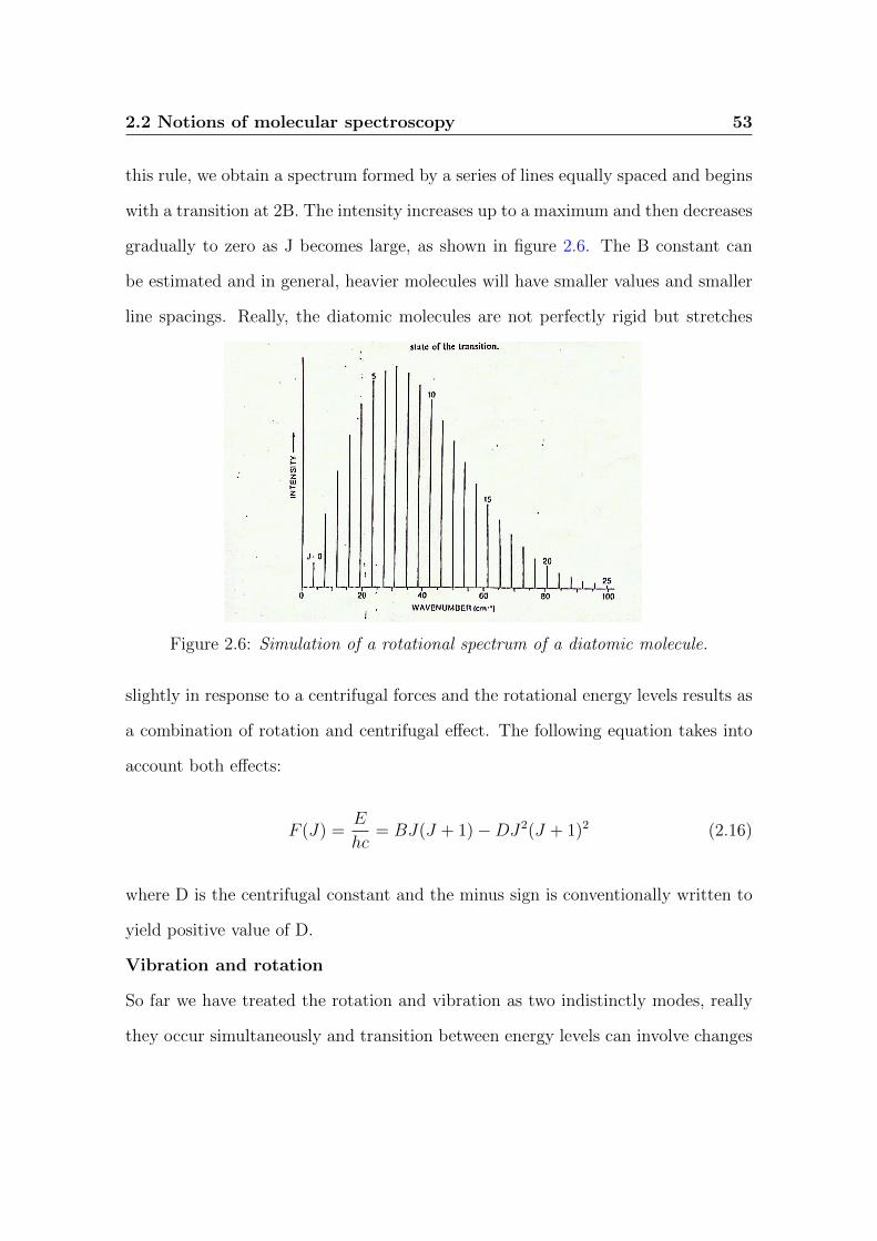
2.2 Notions of molecular spectroscopy 53
this rule, we obtain a spectrum formed by a series of lines equally spaced and begins
with a transition at 2B. The intensity increases up to a maximum and then decreases
gradually to zero as J becomes large, as shown in figure 2.6. The B constant can
be estimated and in general, heavier molecules will have smaller values and smaller
line spacings. Really, the diatomic molecules are not perfectly rigid but stretches
Figure 2.6: Simulation of a rotational spectrum of a diatomic molecule.
slightly in response to a centrifugal forces and the rotational energy levels results as
a combination of rotation and centrifugal effect. The following equation takes into
account both effects:
F (J) =E
hc= BJ(J + 1)−DJ2(J + 1)2 (2.16)
where D is the centrifugal constant and the minus sign is conventionally written to
yield positive value of D.
Vibration and rotation
So far we have treated the rotation and vibration as two indistinctly modes, really
they occur simultaneously and transition between energy levels can involve changes
54 2. Planetary atmospheres and notion of spectroscopy
in both modes. The spectrum consist of vibration transitions plus rotational fine
structure around each of the vibrational wavenumbers. As a first approximation the
rotational energy is given by a combination of rotation plus vibration plus centrifugal
distortion, as shown bellow:
F (ν, J) = ν0(ν +1
2)− ν0a(ν +
1
2)2 +BJ(J + 1)−DJ2(J + 1)2 (2.17)
where ν0= ω2πc
is the classical vibration wavenumber. The frequency of vibration
states is typically much higher than that of rotation, so that the B value results
from an average molecular configuration and moment of inertia, as the dimensions
change during vibration. B is a function of vibrational state and decreases as ν
increases. When the molecule rotates the stretching distortion of the internuclear
separation is characterized by D and this effect will change from one vibrational
state to another. We have an interaction between vibration and rotation states and,
for this reason, the D is also function of the quantum number ν.
Finally, we obtain a complex expression of the energy that takes into account all
effects and following shown:
F (ν, J) = ν0(ν +1
2)− ν0a(ν +
1
2)2
+B0J(J + 1)− α(ν +1
2)J(J + 1)
−D0J2(J + 1)2 − β(ν +
1
2)J2(J + 1)2
(2.18)
The rotational energy level structure in each vibrational state (see last two terms
in equation 2.18), is similar to the form of the equation 2.16, except that the rota-
tional coefficients are now D(ν) and B(ν), i.e. function of the quantum number ν.
A transition between two vibration-rotation energy levels will be accompanied by

2.2 Notions of molecular spectroscopy 55
emission or absorption of a photon at wavenumber:
ν =E ′
hc− E”
hc= F (ν ′, J)− F (ν”, J) (2.19)
where F(ν,J) is given by equation 2.16. Each transition appears in the spectrum as
a band, or set of lines corresponding to the many rotational transitions that may ac-
company a vibrational transition. The separation between rotational lines are much
smaller than the separation between vibrational bands. Each band is centered at its
vibrational wavenumber and is composed of two series of rotational lines, called R
and P branch. The first extends to higher wavenumbers and described by
ν=ν0+2B(J+1) ⇒ for ∆J=+1
The second one, extends toward lower wavenumber and described by
ν=ν0-2B(J+1) ⇒ for ∆J=-1
Lines in P and R branches are separated by approximately by 2B; an example of
spectrum are reported in figure 2.7.
Polyatomic molecules
Figure 2.7: Simulation of ν=1-0 transition of the CO. The band center is at 2143cm−1 and the P and R branches extend toward lower and higher wavenumbers.

56 2. Planetary atmospheres and notion of spectroscopy
Everything has been said so far can be extended to the polyatomic molecules, taking
into account that in this case the molecule vibrates in several modes each with a
different frequency and can rotate around any axis. For the roto-vibrational transi-
tions, we assume that the overall energy is approximately the sum of the vibration
and rotation energies.
Rather than describing in detail the various processes , as we did in the previous
pages,we will report in the following table the main selection rules.
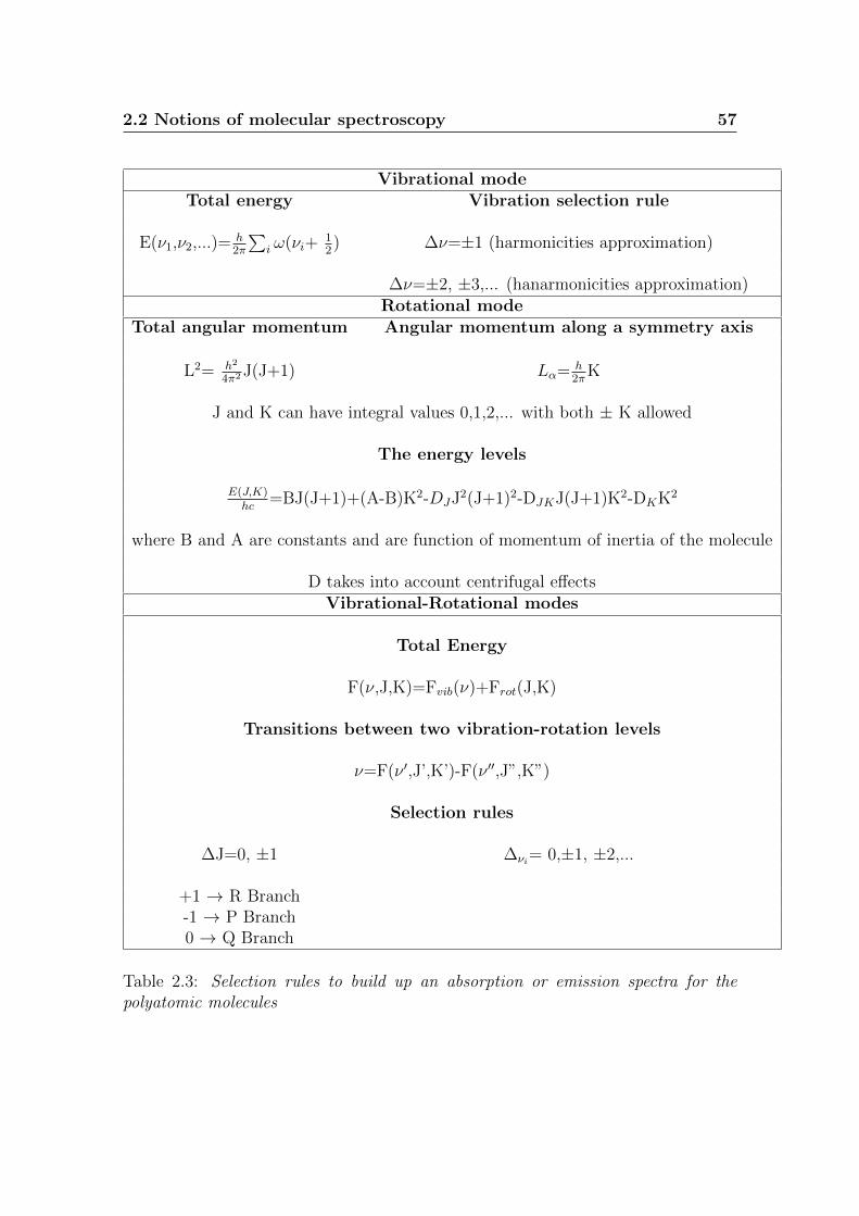
2.2 Notions of molecular spectroscopy 57
Vibrational modeTotal energy Vibration selection rule
E(ν1,ν2,...)= h2π
∑i ω(νi+
12) ∆ν=±1 (harmonicities approximation)
∆ν=±2, ±3,... (hanarmonicities approximation)Rotational mode
Total angular momentum Angular momentum along a symmetry axis
L2= h2
4π2 J(J+1) Lα= h2π
K
J and K can have integral values 0,1,2,... with both ± K allowed
The energy levels
E(J,K)hc
=BJ(J+1)+(A-B)K2-DJJ2(J+1)2-DJKJ(J+1)K2-DKK2
where B and A are constants and are function of momentum of inertia of the molecule
D takes into account centrifugal effectsVibrational-Rotational modes
Total Energy
F(ν,J,K)=Fvib(ν)+Frot(J,K)
Transitions between two vibration-rotation levels
ν=F(ν ′,J’,K’)-F(ν ′′,J”,K”)
Selection rules
∆J=0, ±1 ∆νi= 0,±1, ±2,...
+1 → R Branch-1 → P Branch0 → Q Branch
Table 2.3: Selection rules to build up an absorption or emission spectra for thepolyatomic molecules
58 2. Planetary atmospheres and notion of spectroscopy
Collision-Induced-Absorption
Homonuclear diatomic molecules, such as H2, N2, O2 and so on, have no permanent
dipole moment, and therefore no electric dipole transitions. However, at high pres-
sure and long path length, electric dipole absorption is observed, as we will show
in the chapter 5. This absorption results from a short-time collisional interaction
between molecules. Radiative transitions among rotational, vibrational and trans-
lations states of colliding pairs of molecules can take place, even though they are
not allowed in the isolated molecules. This process is especially important in the at-
mospheres of planets, as Venus and Jupiter. In the latter case, the collision-induced
absorption by molecular hydrogen dominates the far infrared spectrum. During a
collision, a transient dipole moment aries as the electron distribution is distorted
by long-range forces or overlapping charge densities. The shape and intensity of
observed spectra are determined by the induced dipole moment µ(R,r1,r2) and the
interaction potential V(R,r1,r2). R represents the intermolecular separation and r
are the vibrational coordinates of molecule; both µ and V depend on the orienta-
tions of the molecules. The induced dipole moment can arise in collisions between
two molecules (CO2-CO2, as in our case), a molecule and an atom (H2-He) or two
dissimilar atoms (He-Ar). Collision-induced absorption from free pairs of molecules
appear as broad lines or bands located at wavenumbers of the pure rotation or
vibration-rotation transitions in the participating individual molecules.
The absorption in the collision induced features, both free pairs and dimers, grows
in proportion to both the numbers of molecules per volume element and the number
of collision partners. Therefore, collision-induced absorption depends on the prod-
uct of the densities of the partners. When the molecules are the same, CO2-CO2
for example, the absorption depends on the square of the density. The absorption

2.2 Notions of molecular spectroscopy 59
strength also increases at lower temperatures, since this corresponds to higher den-
sities at a given pressure, and because the molecules are thermally distributed over
fewer energy levels.
This behavior is in agreement with the collision-induced-absorption bands observed
in our spectra, as will discussed in section 5.3.
For a detailed description of this phenomenon, refer to [28]

Chapter 3
Experimental setup
The reasons that led us to assemble an experimental setup have already been ex-
plained in the introduction and will be evident in the course of this work. Therefore,
in this chapter a detailed description of the Fourier Transformer InfraRed (FT-IR)
spectrometer and the gas cell that allowed us to recreate in our laboratory the same
conditions found in the deep atmosphere of Venus are given.
3.1 FT-IR interferometer
The CO2 absorption spectra have been recorded with a Bruker-Vertex 80 Fourier
Transform InfraRed (FT-IR) interferometer; an image is shown in figure 3.1.
The technical specifications described in this section are taken from the Vertex 80
user manual [29].
The instrument is equipped with a Tungsten lamp, air-cooled which emits Visible/Near-
InfraRed light and a Globar source that emits Mid-InfraRed light. All external
sources can be connected to one of the two inlet ports, as shown in the figure 3.2.
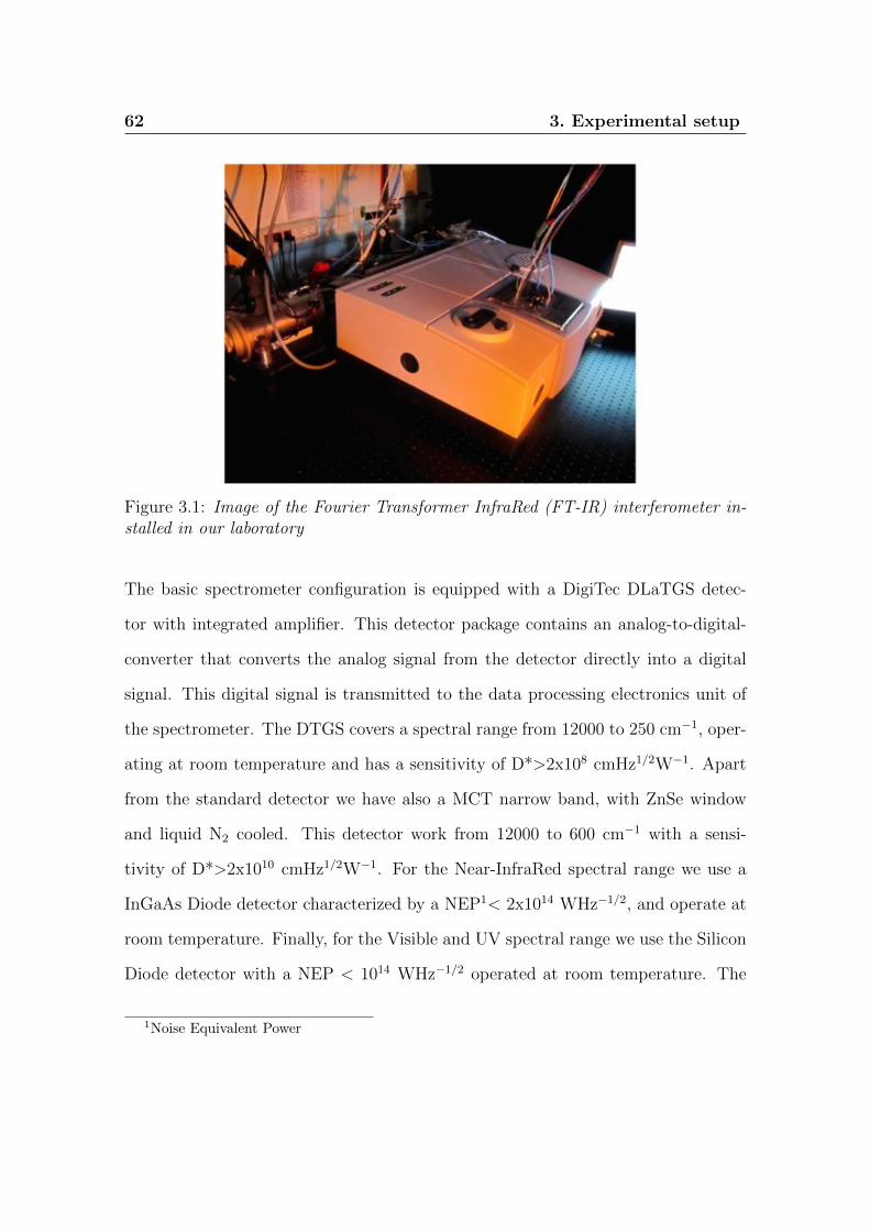
62 3. Experimental setup
Figure 3.1: Image of the Fourier Transformer InfraRed (FT-IR) interferometer in-stalled in our laboratory
The basic spectrometer configuration is equipped with a DigiTec DLaTGS detec-
tor with integrated amplifier. This detector package contains an analog-to-digital-
converter that converts the analog signal from the detector directly into a digital
signal. This digital signal is transmitted to the data processing electronics unit of
the spectrometer. The DTGS covers a spectral range from 12000 to 250 cm−1, oper-
ating at room temperature and has a sensitivity of D*>2x10⁸ cmHz1/2W−1. Apart
from the standard detector we have also a MCT narrow band, with ZnSe window
and liquid N2 cooled. This detector work from 12000 to 600 cm−1 with a sensi-
tivity of D*>2x10¹⁰ cmHz1/2W−1. For the Near-InfraRed spectral range we use a
InGaAs Diode detector characterized by a NEP1< 2x10¹⁴ WHz−1/2, and operate at
room temperature. Finally, for the Visible and UV spectral range we use the Silicon
Diode detector with a NEP < 1014 WHz−1/2 operated at room temperature. The
1Noise Equivalent Power
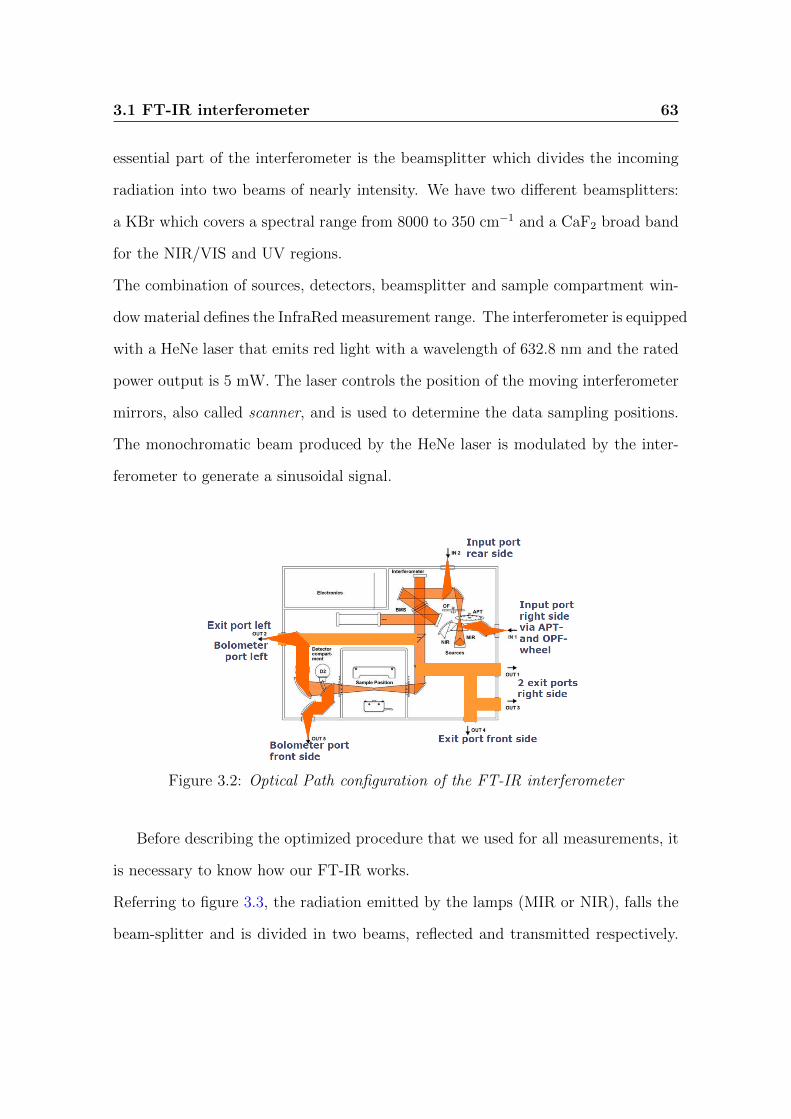
3.1 FT-IR interferometer 63
essential part of the interferometer is the beamsplitter which divides the incoming
radiation into two beams of nearly intensity. We have two different beamsplitters:
a KBr which covers a spectral range from 8000 to 350 cm−1 and a CaF2 broad band
for the NIR/VIS and UV regions.
The combination of sources, detectors, beamsplitter and sample compartment win-
dow material defines the InfraRed measurement range. The interferometer is equipped
with a HeNe laser that emits red light with a wavelength of 632.8 nm and the rated
power output is 5 mW. The laser controls the position of the moving interferometer
mirrors, also called scanner, and is used to determine the data sampling positions.
The monochromatic beam produced by the HeNe laser is modulated by the inter-
ferometer to generate a sinusoidal signal.
Figure 3.2: Optical Path configuration of the FT-IR interferometer
Before describing the optimized procedure that we used for all measurements, it
is necessary to know how our FT-IR works.
Referring to figure 3.3, the radiation emitted by the lamps (MIR or NIR), falls the
beam-splitter and is divided in two beams, reflected and transmitted respectively.

64 3. Experimental setup
Figure 3.3: Simplified schematization of an Fourier interferometer
The reflected beam falls a plane fixed mirror M1, at a distance L, and back towards
the beam splitter. The total optical path that the beam travels is 2L. The trans-
mitted beam falls a movable plane mirror M2. As this mirror moves back and forth
around L by a distance ∆x, the total path is 2(L+∆X) long. The beams, returning
from the two mirrors, are recombined at the beam splitter and, when reach the
detector, they have traversed different optical paths with a path difference δ=2∆x.
The beams are spatially coherent and interfere with each other when recombined.
The FT-IR splits and recombined the two beams with relative phase difference that
depends on the mirror displacement, or optical retardation.
If δ =0, λ, 2λ,. ... the two beams interfere constructively at the detector yielding a
maximum signal.
If δ=λ2, 3λ
2, 5λ
2,....the two beams interfere destructively yielding a minimum signal.
The complete functional relationship between the intensity I and the path difference
∆x is
I(∆(x)) = S(ν) ∗ cos(2πνδx) (3.1)
where ν is the wave number and S(ν) is the intensity of a monochromatic spectral
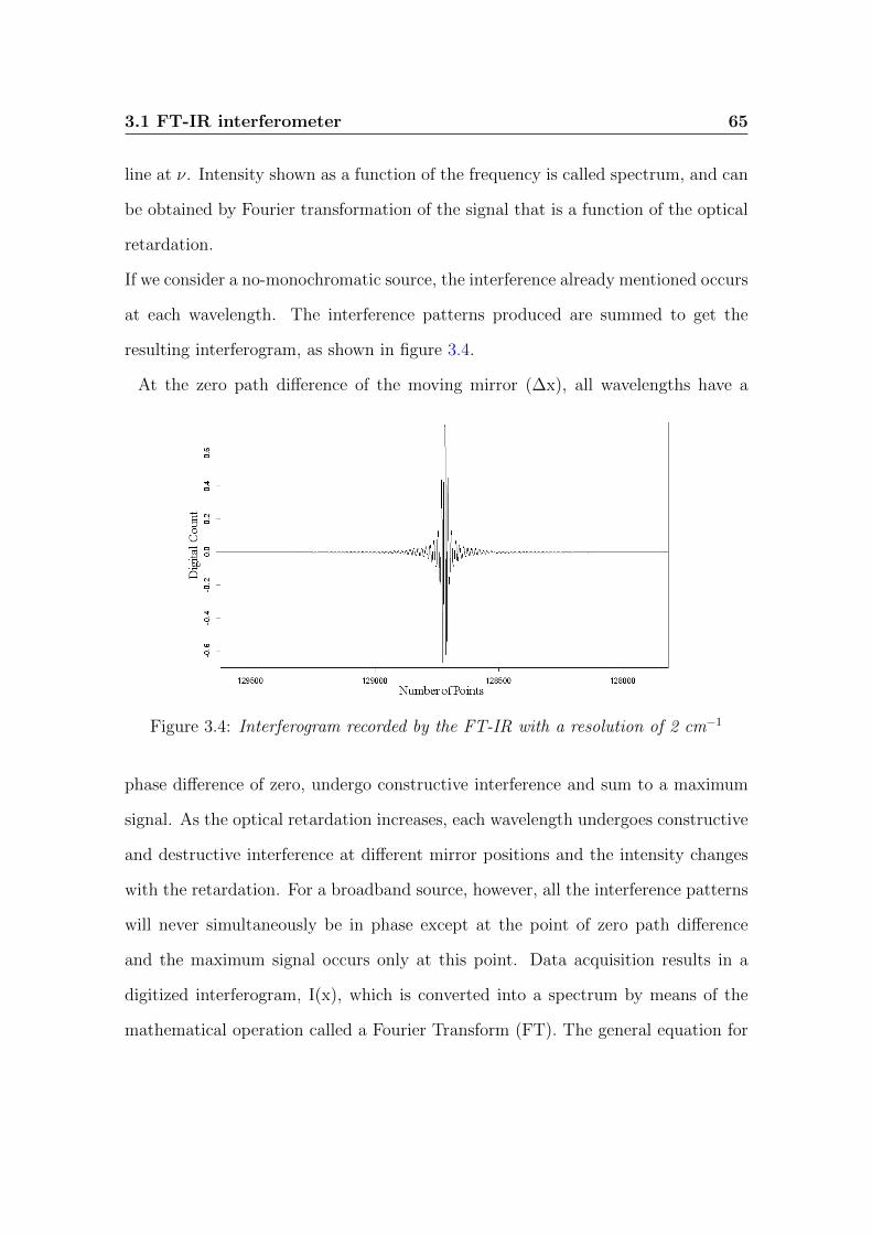
3.1 FT-IR interferometer 65
line at ν. Intensity shown as a function of the frequency is called spectrum, and can
be obtained by Fourier transformation of the signal that is a function of the optical
retardation.
If we consider a no-monochromatic source, the interference already mentioned occurs
at each wavelength. The interference patterns produced are summed to get the
resulting interferogram, as shown in figure 3.4.
At the zero path difference of the moving mirror (∆x), all wavelengths have a
Figure 3.4: Interferogram recorded by the FT-IR with a resolution of 2 cm−1
phase difference of zero, undergo constructive interference and sum to a maximum
signal. As the optical retardation increases, each wavelength undergoes constructive
and destructive interference at different mirror positions and the intensity changes
with the retardation. For a broadband source, however, all the interference patterns
will never simultaneously be in phase except at the point of zero path difference
and the maximum signal occurs only at this point. Data acquisition results in a
digitized interferogram, I(x), which is converted into a spectrum by means of the
mathematical operation called a Fourier Transform (FT). The general equation for

66 3. Experimental setup
the FT is applicable to a continuous signal. If the interferogram is digitized, and
consist of N discrete, equidistant points, the equation 3.1 becomes:
S(K∆ν) =∑
I(n∆x)exp
(i2πnK
N
)(3.2)
where n is the discrete interferogram points and K the discrete spectrum points.
The fact that we now have a discrete, rather than continuous, function and that it’s
only calculated for a limited range of n, leads to important effects, named Picket-
fence effect and leakage. This effect occurs if the interferogram contains frequency
components which do not exactly coincide with the data point position k*ν in the
spectrum. This can be reduced by adding zeros to the end of the interferogram
before the FT is performed. This manipulation increases the number of points per
wavenumber and reduces the error caused by the picket-fence effect. In our case,
the original interferogram size should always be at least doubled by zero filling, i.e.
zero filling factor of two is chosen.
In a real measurement, the interferogram can only be measured for a finite distance
of mirror travel. The resulting can be thought as an infinite length interferogram
multiplied by a rectangular function, i.e. a function that is equal 1 in the range of
measurement and 0 elsewhere. The solution to the leakage problem is to truncate the
interferogram less abruptly. This can be achieved by multiplying the interferogram
by a function that is 1 at the zero path difference and close to 0 at the end of this.
This is called apodization function and in the specific case, we used a Blackman-
Harris [30] function whose expression is given by:
ω(n) = a0 − a1 cos
(2πn
N − 1
)+ a2 cos
(4πn
N − 1
)− a3 cos
(6πn
N − 1
)(3.3)

3.1 FT-IR interferometer 67
where a0=0.35875, a1=0.48829, a2=0.14128, a3=0.01168.
Both optical and electronic effects, can produce a shift of the interferogram phase
because the sinusoidal interference patterns of different wavelengths are slightly
shifted with respect to each other. These phase shift lead to asymmetry in the
interferogram, which is corrected during the Fourier Transform using a Mertz [31]
phase correction.
There are many advantages for using an interferometer, the main ones are:
• The sampling interval of the interferogram, δx, is the distance between zero
crossing of the HeNe laser, and is therefore precisely determined by the laser
wavelength. Since the point spacing in the resulting spectrum, δν, is in-
versely proportional to δx, FT-IR spectrometers have an intrinsic highly pre-
cise wavenumber scale. This advantage is known as Connes’ advantage.
• The Jacquinot advantage aries from the fact that the circular apertures used
in the FT-IR spectrometers have a large area than the slits used in grating
spectrometer, thus enabling higher throughput of radiation.
• In the grating spectrometers the spectrum S(ν) is measured directly by record-
ing the intensity at successive, narrow, wavelength ranges. In FT-IR all wave-
lengths from the sources impinge simultaneously on the detector. This leads
to the multiplex, or Fellgett’s, advantage.
The last statement, does not apply to VIRTIS, because the different wavelengths
come and are sampled simultaneously at the focal plane.
The combination of the Jacquinot and Fellgett advantages means that the signal to

68 3. Experimental setup
noise ratio of the FT-IR spectrometer can be more than 10 times that of a dispersive
spectrometer.

3.2 Gas cell 69
3.2 Gas cell
The FT-IR has been integrated with a special customized high pressure-high tem-
perature (HP-HT) gas cell. In figure 3.5, you can see a picture of the cell and a
diagram showing the breakdown of the cell into three parts connected by a special
viton 2 O-rings.
The technical specifications described in this section are taken from the AABSPEC
] 2T-AWT user manual [32]
2Fluorocarbon elastomers are highly fluorinated carbon-based polymers used in applications toresist harsh chemical and ozone attack. The working temperature range is considered to be -26Cto +205/230C
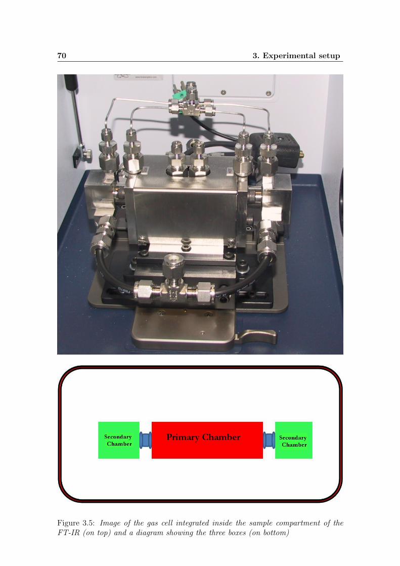
70 3. Experimental setup
Figure 3.5: Image of the gas cell integrated inside the sample compartment of theFT-IR (on top) and a diagram showing the three boxes (on bottom)
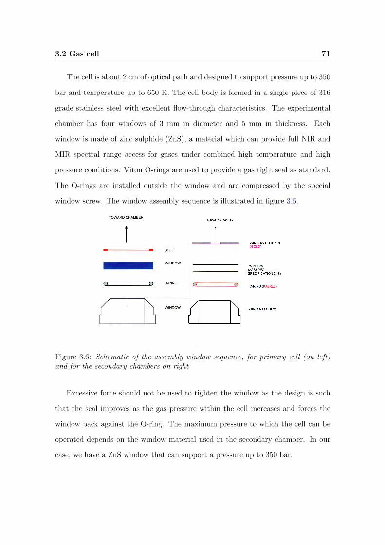
3.2 Gas cell 71
The cell is about 2 cm of optical path and designed to support pressure up to 350
bar and temperature up to 650 K. The cell body is formed in a single piece of 316
grade stainless steel with excellent flow-through characteristics. The experimental
chamber has four windows of 3 mm in diameter and 5 mm in thickness. Each
window is made of zinc sulphide (ZnS), a material which can provide full NIR and
MIR spectral range access for gases under combined high temperature and high
pressure conditions. Viton O-rings are used to provide a gas tight seal as standard.
The O-rings are installed outside the window and are compressed by the special
window screw. The window assembly sequence is illustrated in figure 3.6.
Figure 3.6: Schematic of the assembly window sequence, for primary cell (on left)and for the secondary chambers on right
Excessive force should not be used to tighten the window as the design is such
that the seal improves as the gas pressure within the cell increases and forces the
window back against the O-ring. The maximum pressure to which the cell can be
operated depends on the window material used in the secondary chamber. In our
case, we have a ZnS window that can support a pressure up to 350 bar.

72 3. Experimental setup
With this gas cell we can reach high pressure and high temperature because while
the primary chamber windows operate at the system temperature and pressure, it is
possible by pressuring the secondary chamber to arrange a near zero pressure drop
across the primary windows. The pressure differential is then handled by secondary
windows which are maintained at near ambient temperature by the cooling system
in the secondary window region. The latter have their full mechanical strength as
they are maintained in the temperature range from 294K to 330K. The secondary
chambers should be pressurized using a low thermal conductivity inert gas, such
as Argon. The gas should enter through the port furthest away from the primary
chamber. If we are flushing the secondary box during high temperature operation
of the gas cell, then we can be sure the gas is cooled before entering the second
secondary chamber. The double chamber design also provides inherently greater
safety for hazardous sample materials.
The gas cell must be powered from a stable source of 120V, 60Hz supply voltage,
which should be stable better than ±1%. Unstable supply voltage may significantly
shorten the operational life of the heater.
To control the temperature of the primary cell we use an ”AABSPEC” Digital Tem-
perature Controllers and Programmers, see the figure 3.7. The technical specifica-
tions described in this section are taken from the AABSPEC ] DTC-1 user manual
[33].
Power is controlled by ”time proportional control” with a one second (nominal)
cycle, switching at zero crossover with so-called fail-safe circuitry. The controller
takes its control temperature reading from a type K chromel-alumel thermocouple
through a non-reversible connector. AABSPEC Controllers and Programs contain
an additional safety feature to give an audible warning in the event of a failure in the
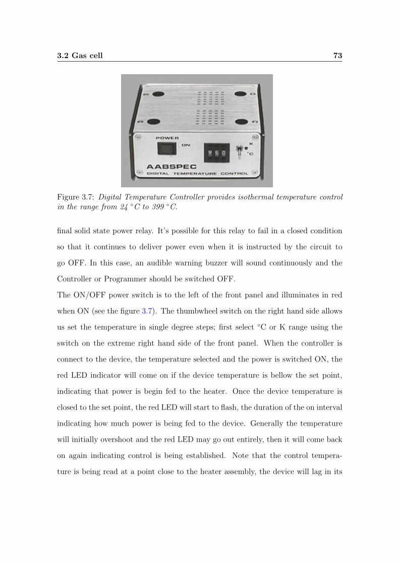
3.2 Gas cell 73
Figure 3.7: Digital Temperature Controller provides isothermal temperature controlin the range from 24 C to 399 C.
final solid state power relay. It’s possible for this relay to fail in a closed condition
so that it continues to deliver power even when it is instructed by the circuit to
go OFF. In this case, an audible warning buzzer will sound continuously and the
Controller or Programmer should be switched OFF.
The ON/OFF power switch is to the left of the front panel and illuminates in red
when ON (see the figure 3.7). The thumbwheel switch on the right hand side allows
us set the temperature in single degree steps; first select C or K range using the
switch on the extreme right hand side of the front panel. When the controller is
connect to the device, the temperature selected and the power is switched ON, the
red LED indicator will come on if the device temperature is bellow the set point,
indicating that power is begin fed to the heater. Once the device temperature is
closed to the set point, the red LED will start to flash, the duration of the on interval
indicating how much power is being fed to the device. Generally the temperature
will initially overshoot and the red LED may go out entirely, then it will come back
on again indicating control is being established. Note that the control tempera-
ture is being read at a point close to the heater assembly, the device will lag in its

74 3. Experimental setup
temperature response to the control temperature reading. For this reason, many
AABSPEC device provide us with the facility to install a read-out thermocouple to
monitor actual device temperature.
The temperature stability will be affected by the stability of the electrical supply
voltage which should be stable better than ± 1 %. Other factors which will affect
temperature stability include heat loss, for example stability of the cooling fluid
temperature and circulation rate.
3.2.1 Connections and calibrations of the set up
As with all control systems, the actual sample temperature is weakly different from
the set point and we had to calibrate our experimental setup.
To do this, we installed a type-K thermocouple inside the central box of the gas
cell, to read the exact gas temperature. The thermocouple consists of two different
conductors (usually metal alloys) that produce a voltage proportional to a tem-
perature difference between either end of the pair of conductor. This sensor has
been connected to a Data Acquisition (DAQ), a particular device able to measure
an electrical or physical phenomenon such as voltage, current, temperature, pres-
sure, or sound. In figure 3.8 you can see a schematic electrical connection between
thermocouple, Data Acquisition and display.
By a program written in LabView (Laboratory Virtual Instrumentation Engi-
neering Workbench) language we read and save the values of gas temperature.
LabView is a graphical programming environment used by engineers and scientists
to develop sophisticated measurement, test and control systems. It offers unrivaled
integration with thousands of hardware devices and provides hundreds of built-in
libraries for advanced analysis and data visualization - all for creating virtual in-
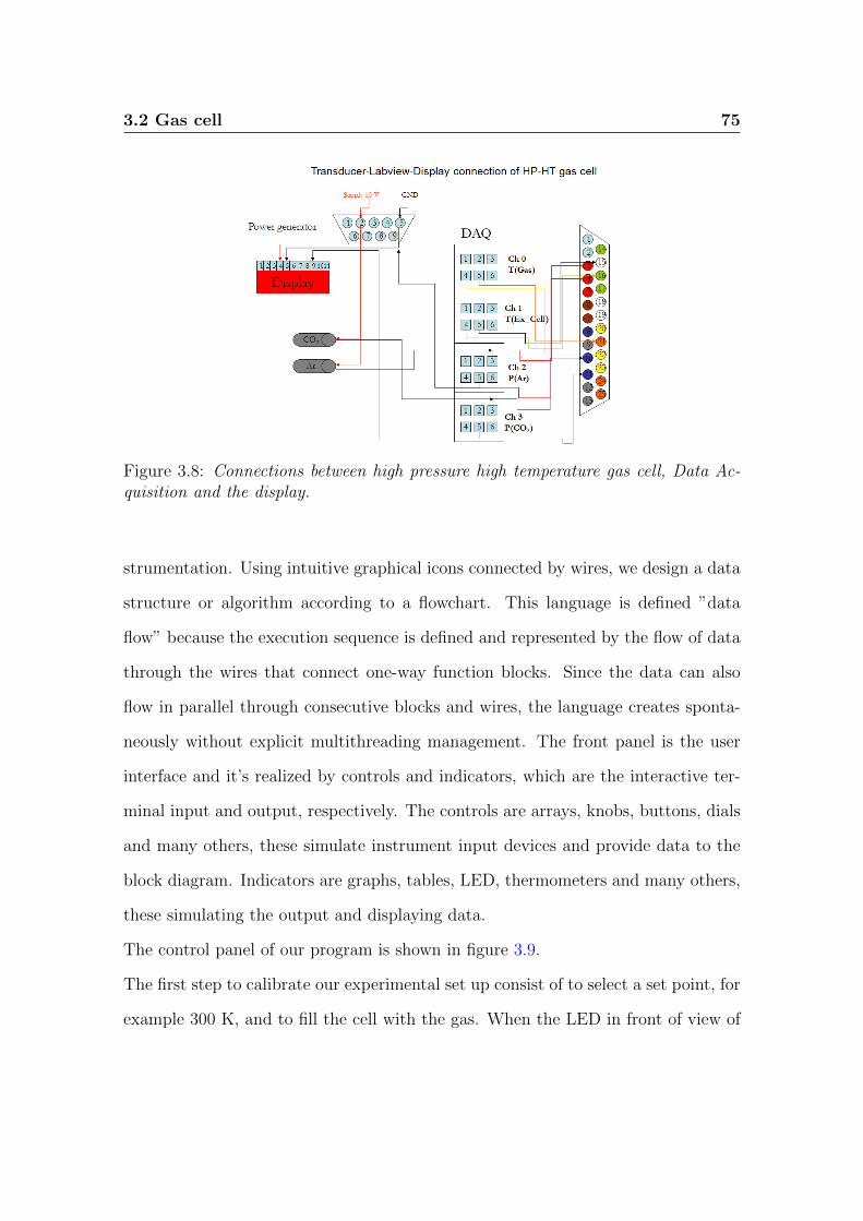
3.2 Gas cell 75
Figure 3.8: Connections between high pressure high temperature gas cell, Data Ac-quisition and the display.
strumentation. Using intuitive graphical icons connected by wires, we design a data
structure or algorithm according to a flowchart. This language is defined ”data
flow” because the execution sequence is defined and represented by the flow of data
through the wires that connect one-way function blocks. Since the data can also
flow in parallel through consecutive blocks and wires, the language creates sponta-
neously without explicit multithreading management. The front panel is the user
interface and it’s realized by controls and indicators, which are the interactive ter-
minal input and output, respectively. The controls are arrays, knobs, buttons, dials
and many others, these simulate instrument input devices and provide data to the
block diagram. Indicators are graphs, tables, LED, thermometers and many others,
these simulating the output and displaying data.
The control panel of our program is shown in figure 3.9.
The first step to calibrate our experimental set up consist of to select a set point, for
example 300 K, and to fill the cell with the gas. When the LED in front of view of

76 3. Experimental setup
Figure 3.9: Panel of control of the program written in LabView to acquire pressureand temperature values.
the controller (see the figure 3.7) start to flash, we are sure that the cell reached the
set point temperature. To obtain a calibration curve of our sensor, we varied the set
point value from 294 to 600 K with a step of 10 K. For each point of this calibration
curve, we record the temperature read by the thermocouple. The calibration curve
has been implemented within the acquisition program and it’s used automatically
to determine the correct set point. For example, in order to have a gas temperature
of 370 K we push the Go button (see figure 3.9) and a second window appears, as
shown in figure 3.10. Once the temperature value in the ”Desired Gas Temperature”
is set, we obtain the adjusted temperature to set in the controller (Set T control @)
and the final gas temperature (Goal Gas Temperature) is correctly reached.
A second thermocouple has been installed outside the cell to monitor the temper-
ature in order to check that it is always at room temperature. This value is also
recorded, as shown in figure 3.9 (outside cell), and for each measurement this tem-
perature is typically less than 30C.

3.2 Gas cell 77
Figure 3.10: Panel of control to select the temperature of the gas.
To insert the CO2 and Argon gases inside the gas cell, we built up a pipes system
connecting the gas bottles with the cell. This system consists of seamless tubing of
1/16” in diameter and 0.014” in thickness, valves and reducing union. Along the
line we insert two gauges, EPXT-PO type, which measure the pressure of gases with
an accuracy better than ± 0.1% on the full range (from 1 to 100 bar). Also in this
case, we record the pressure values read from gauges as shown in figure 3.9.

78 3. Experimental setup
3.2.2 Measurements procedure
To obtain the gas transmittance, the procedure is as follows: the central box is
heated up to the target of temperature, for example 373 K, while the lateral part
is maintained cold. The three chambers are filled with Argon (Ar) at the preset
pressure, and the background radiance R(ν) is recorded. We chose the argon as the
reference spectrum, because there are no bands in the spectral region of our interest.
Afterwards the Ar in the central section is replace by CO2 at the preset pressure
and the radiance with the absorption spectrum S(ν) is recorded. An example of
background and sample radiance is shown in figure 3.11.

3.2 Gas cell 79
Figure 3.11: Background and absorption spectrum radiance (from the top down tothe bottom) recorded with a resolution of 2 cm−1 and Ar and CO2 at p∼11 bar andT∼513K respectively.

80 3. Experimental setup
The transmittance T(ν) is obtained such as ratio between S(ν) and R(ν) as
shown in the following expression:
T (ν) =S(ν)
R(ν)(3.4)
The same procedure has been applied to all measurements.
In the field of planetary sciences, it is customary to speak of absorbance or ab-
sorption coefficients rather than transmittance.Therefore, the CO2 absorption
coefficients, being defined as
Absorbance(ν) = − ln(T )
l(cm−1) (3.5)
where l is the optical path, which in our case is (2±0.03) cm along.
We have optimized this procedure to remove the emission of the water vapour and
CO2 along the optical path of the FT-IR. in addition, working at very high pressures,
we must monitoring the pressure gradients that act on the windows of the gas cell.

Chapter 4
Radiative transfer models
In principle, all the measured data (earth based, airborne, from space, in labora-
tory) would be completely useless without any good theoretical model to convalidate
them. The opposite is true as well. A model can be said a good model if it is veri-
fied by observations. New scientific knowledge occurs only when those two distinct
aspects are in agreement with each other, becoming the same thing.
In this chapter three different models that were used to obtain the synthetic spectra
will be described. These were then compared with our experimental data. Compar-
ison and discussion on the results are reported in chapter 5.
The first model is based on the Atmosphere Radiation Spectrum (ARS). It is
a set of routines implementing line by line calculation of gases and aerosol opacity,
transmittance, and atmospheric radiance spectra. The second one, named Solu-
tion, is a line shape models valid at high pressure and takes into account two
different mechanisms: ”line mixing” and ”far wings”. The last one, called Line
Mixing Model (LMM), is a different approach to the lines interferences due to
inter-molecular collisions (or ”line mixing”) which have a very important influence

82 4. Radiative transfer models
on the spectral shape.
4.1 ARS: Model and Software
This code is a set of routines written in fortran 77 and C able to perform computa-
tions of several physical quantities and to solve the radiative transfer equation under
different conditions. Using different packages separately, the code can compute the
opacity of gaseous species and aerosols, the transmittance and the radiance spectra
with only LTE 1 conditions [34]. The code was originally created and developed
by N.I. Ignatiev (IKI RAN-Moskow) to study the data of the Planetary Fourier
Spectrometer (PFS), instrument of the Mars Express mission’s, but it’s now used
for other planetary atmospheres by many research teams. In general the radiative
transfer problem can be subdivided in two distinct and independent tasks: compu-
tation of physical properties and solution of the radiative transfer equation itself.
From a informatics point of view, ARS uses many packages and modules. Every
package requires a set of initialization files (*.ini) and as sequential boxes, the out-
put of the previous box is the input of the subsequent one. The main packages can
be summarized as follow:
• Arshls : this package extracts spectral lines data from a spectroscopic database
and converts them into a reduced format file. It is able to change isotopic
ratios and Lorentz line half widths. Moreover it can discard all the lines with
intensity lower than a chosen value. Another important option is the line wings
cutoff, in order to consider the main contribution of the information only. It
1Local Thermodynamical Equilibrium: In thermodynamics, a thermodynamic system is said tobe in local thermodynamic equilibrium when it is in thermal, mechanical, radiative and chemicalequilibrium

4.1 ARS: Model and Software 83
can work with different databases also.
• Arsv : once the lines are extracted, the next important step is the creation of a
grid with different resolutions. This package can create uniform or combined
wavenumber grid, according to different line parameters (positions, widths,
strengths, line shape, etc...) in wavenumber units only. It is possible to have
uniform spectral range or combine ranges of different resolution. Because the
very different number of lines in different parts of a selected spectral range,
this last option can be very useful in order to save computational time.
• Arsk : this module of ARS is the real first step to the radiative quantities
calculation. It computes gaseous absorption coefficients on the specified res-
olution grid using all the spectroscopic parameters calculated by Arshls and
interpolates absorption coefficients for any temperature and pressure profile
defined by the user. The outputs of this package are used by the next module.
• Arsm :this is the main package of ARS. It handles all the monochromatic
quantities calculated by Arsk (and Arshls) and solves the radiative transfer
equation under different conditions, as said before. In particular it calculates
transmittance, radiance and fluxes inside and outside the atmosphere taking
into account both single and multiple scattering. The diffusion and emission
of the aerosols and the presence of clouds are taken into account in this step.
After a brief description of the software, the role of each single package and how
they work together to obtain the final spectra is presented.

84 4. Radiative transfer models
4.1.1 What does the program do
Absorption coefficients
First step is the extraction of important spectroscopic parameters from a database.
ARS was designed to work mainly with HITRAN [1]. Basically it’s a data archive
where information on molecular spectral lines are stored in. Arshls extracts the
line data from it and converts it into a reduced format. Moreover, it is possible
to work with others HITRAN-like databases, if they have a similar data format.
Before extracting line data, the user can define many parameters as line intensity,
line width and the shape of the line, the isotopes (if any), a different broadening
(non-terrestrial atmosphere), wings line and/or weak lines cut-off. In detail, the
quantities taken by Arshls from the database for each single line are:
• ν0 central position of the line in [cm−1] and atmospheric standard conditions:
T0 = 296K, p0 = 1 atm
• S(T0): line intensity at Temperature T0
• αair(p0, T0): selected gaseous molecule broadening due to the atmospheric en-
vironment
• αself (p0, T0): selected gaseous molecule broadening due to itself
• E”: transition lower state energy in [cm−1]
• m: exponential index HWHM (Half Width at Half Maximum) Lorentz’s line
shape vs. temperature ratio
From those informations, the absorption of gaseous species can be computed. The
absorption coefficient is the final output parameter of the Arsk package. It works

4.1 ARS: Model and Software 85
on the grid created by the user with Arsv which creates an optimized wavenumber
grid according with positions, widths and strengths of the lines. Arsk takes into
account different steps before coming to the final gaseous absorption coefficient.
The mathematical expression for the line intensity is defined as follow:
S(T ) = S(T0)Q(T0)
Q(T )exp
[−c2E
′′(
1
T− 1
T0
)]1− exp
(c2ν0T
)1− exp
(c2ν0T0
) (4.1)
where S(T0) is the line strength at standard temperature conditions
Q(T) is the full statistical partition sum 2
T is the air profile temperature defined by the user
and c2 = hcKb
.
The molecular absorption cross-section in cm2 per molecule in a spectral line with
Voigt line shape is given by the formula :
σν =Sa
π23β
∫ +∞
−∞
exp−t2dta2 + (x− t)2
(4.2)
with
a =α
βand x = ν − ν0 (4.3)
where S is the line intensity, ν0 is the line center, α is the Lorentz half width, β is
the doppler half width, defined as
β =ν0
c
√2RT
M(4.4)
2Rotational and vibrational energy contributions are both here included
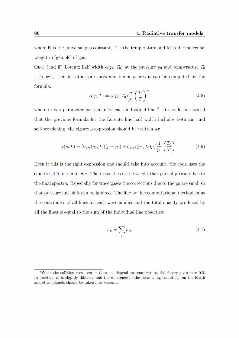
86 4. Radiative transfer models
where R is the universal gas constant, T is the temperature and M is the molecular
weight in [g/mole] of gas.
Once (and if) Lorentz half width α(p0, T0) at the pressure p0 and temperature T0
is known, then for other pressures and temperatures it can be computed by the
formula:
α(p, T ) = α(p0, T0)p
p0
(T0
T
)m(4.5)
where m is a parameter particular for each individual line 3. It should be noticed
that the previous formula for the Lorentz line half width includes both air- and
self-broadening, the rigorous expression should be written as:
α(p, T ) = [αair(p0, T0)(p− ps) + αself (p0, T0)ps]1
p0
(T0
T
)m(4.6)
Even if this is the right expression one should take into account, the code uses the
equation 4.5 for simplicity. The reason lies in the weight that partial pressure has to
the final spectra. Especially for trace gases the corrections due to the ps are small so
that pressure line shift can be ignored. The line by line computational method sums
the contributes of all lines for each wavenumber and the total opacity produced by
all the lines is equal to the sum of the individual line opacities:
σν =∑i
σνi (4.7)
3When the collision cross-section does not depend on temperature, the theory gives m = 0.5.In practice, m is slightly different and the difference in the broadening conditions on the Earthand other planets should be taken into account.

4.2 Solution 87
from this relation the absorption coefficient can be easily obtained as:
kν = σνn (4.8)
where n = p/KbT is the number density coming from the perfect gases law. It is
important to notice that the absorption data which are stored by Arsk program in
the output file are obtained per unit path length and for 100% pure gas.
4.2 Solution
This software, written by the group of the A.V. Rodin (IKI RAN-Moskow), is a
line shape models valid at high pressure, when the shape of spectral lines no longer
follows the conventional Lorentzian profile. Two mechanisms are thought to be re-
sponsible for this effect: ”line mixing” [35], or interference of rotational states when
individual rotational lines overlap; and dense, short-pathlengths intermolecular col-
lisions [36], which determine far wings of spectral lines and are believed to reveal
non-Poisson statistics.
In this section, the two effects will be treated separately.
4.2.1 Line Mixing effect
When we are in a typical terrestrial conditions, the behavior of gases is well described
by the ideal gas law. Vice-versa, when we study the optical properties of gases at
high pressure and high temperature, such as those found in the deep atmosphere of
Venus, this approximation falls. In this case, we assume that the behavior of the

88 4. Solution Code
gas is well described by the Wan der Waals law. From a spectroscopic point of view,
we have that the average distances between the molecules are comparable to the
molecule size, and molecules spend most of their time interacting with each other.
This means that the effective energy levels of an ensemble of molecules overlap. It
makes sense to consider the vibrational band profile instead of the line profile. This
simplest approximation is the strong collision approximation, which suggest
that the lifetime does not depend on the rotational state and is averaged over the
vibrational band. Referring to the ”Petersburg model” [37] and considering what
we have just said, let’s to calculate the absorption coefficients.
The net spectral absorption coefficient k(ν), is a superposition of the absorption
produced by transition between different vibrational states:
k(ν) =∑j
F
(∑i
Si,jf(ν − νi,∆Li ,∆
D)
)(4.9)
where j is the index of sum over the bands, i the index of the rotational transition, ∆L
and ∆D are the homogeneous (collisional) and inhomogeneous (Doppler) broadening
factors and Si,j is the oscillator strength. If we consider molecular absorption of
a particular vibrational band, consisting of N ro-vibrational transitions with line
strengths for given temperature Si and wavenumbers νi, spontaneous transition rate
for each line is:
Ai =Si
ν ∗ (1− eKcνiKT )
(4.10)
For the entire band, the total probability is:
As =∑i
Ai (4.11)
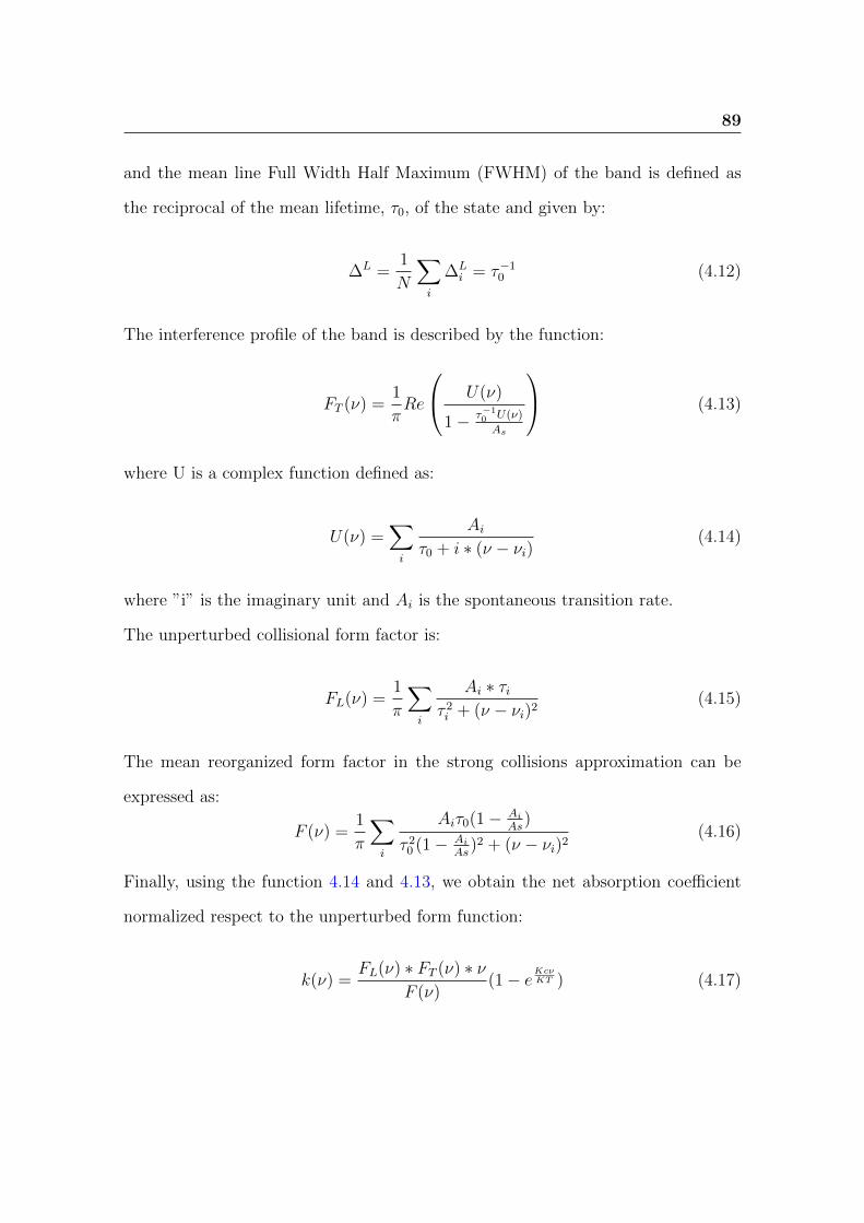
89
and the mean line Full Width Half Maximum (FWHM) of the band is defined as
the reciprocal of the mean lifetime, τ0, of the state and given by:
∆L =1
N
∑i
∆Li = τ−1
0 (4.12)
The interference profile of the band is described by the function:
FT (ν) =1
πRe
U(ν)
1− τ−10 U(ν)
As
(4.13)
where U is a complex function defined as:
U(ν) =∑i
Aiτ0 + i ∗ (ν − νi)
(4.14)
where ”i” is the imaginary unit and Ai is the spontaneous transition rate.
The unperturbed collisional form factor is:
FL(ν) =1
π
∑i
Ai ∗ τiτ 2i + (ν − νi)2
(4.15)
The mean reorganized form factor in the strong collisions approximation can be
expressed as:
F (ν) =1
π
∑i
Aiτ0(1− AiAs
)
τ 20 (1− Ai
As)2 + (ν − νi)2
(4.16)
Finally, using the function 4.14 and 4.13, we obtain the net absorption coefficient
normalized respect to the unperturbed form function:
k(ν) =FL(ν) ∗ FT (ν) ∗ ν
F (ν)(1− e
KcνKT ) (4.17)

90 4. Solution Code
The absorption coefficient of a molecular gas is then obtained by adding absorption
values caused by all vibrational bands. Not only bands falling into considered spec-
tral range should be taken into account, but also bands whose centers are far apart.
Note that in this approach, individual lines are no longer considered separately, in-
stead, the whole band obeys its own shape. We have to remember that at normal
pressures and temperatures, the band profile converges to the classical Lorentz form
factor.
4.2.2 Far Wings approximation
As just said in section 4.2.1, under extreme conditions the perfect gas approximation
falls and also the broadening of spectral lines is different from the ordinary Lorentz
contour. The interference of molecular states is the basic physical effect determining
absorption in very dense gases. Also, the main contribution to the absorption is
provided by transition between the unperturbed energy levels of an isolated molecule
and that the line broadening is formed due to intermolecular collisional interaction.
According to the ”Tomsk model” [38], we assume that far wing profile is formed in
dense collisions and is determined by the rapidly growing region of the potential of
the intermolecular interaction. The dependence of form-factor on thermodynamic
conditions is determined by a classical statistical problem. Now, let us consider an
isolated spectral line at a frequency ν0, the entire spectral interval is divided into
four regions. The Voigt shape is assumed for the inner region, while for the other
parts of the band, the line shape is described by the relationship:
f =Ds ∗ δ ∗ ω
Rs(ω − ω0)(1+ 3As
)
∫ Rs
0
exp(−ε((σr)12 − (σ
r)6) hc
KT√R2s − r2
rdr (4.18)

91
where
Rs =Cs
(ω − ω0)1As
(4.19)
the constants As, Cs and Ds parameterize all quantum-mechanical effects and do
not depend on thermodynamical conditions. The important parameters are also ε
and σ, which occur in the expression for the Lennard Jones potential [39] of the
intermolecular interaction and vary with temperature. In particular, ε is the depth
of the potential well and σ is the finite distance at which the inter-particle potential
is zero. The model line profile is schematically shows in figure 4.1.
Figure 4.1: Model spectral line profile
The most important parameters, necessary to draw the line profile, are the
boundaries ω1,ω2 and ω3 of the regions where the behavior of the form factor changes.
These values are determined by the condition that the approximation by form factor
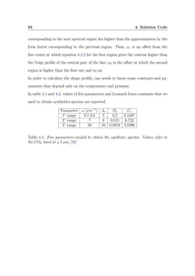
92 4. Solution Code
corresponding to the next spectral region lies higher than the approximation by the
form factor corresponding to the previous region. Thus, ω1 is an offset from the
line center at which equation 4.2.2 for the first region gives the contour higher than
the Voigt profile of the central part of the line; ω2 is the offset at which the second
region is higher than the first one and so on.
In order to calculate the shape profile, one needs to know some constants and pa-
rameters that depend only on the temperature and pressure.
In table 4.1 and 4.2, values of free parameters and Lennard-Jones constants that we
used to obtain synthetics spectra are reported.
Parameter ω (cm−1) As Ds Cs1 range 0.1-3.0 5 0.2 6.54872 range 7 8 0.015 6.7223 range 30 16 0.0053 5.0396
Table 4.1: Free parameters needed to obtain the synthetic spectra. Values refer tothe CO2 band at 4.3 µm [38]

93
Temperature (K) ε σ193.0 904.82 3.8940218.0 859.60 3.9201296.0 760.00 4.0030414.0 699.10 4.0945534.0 718.70 4.1440540.0 560.70 4.2000627.0 686.50 4.2185751.0 682.90 4.2219920.0 479.90 4.4075
Table 4.2: CO2 intermolecular interaction parameters versus temperature
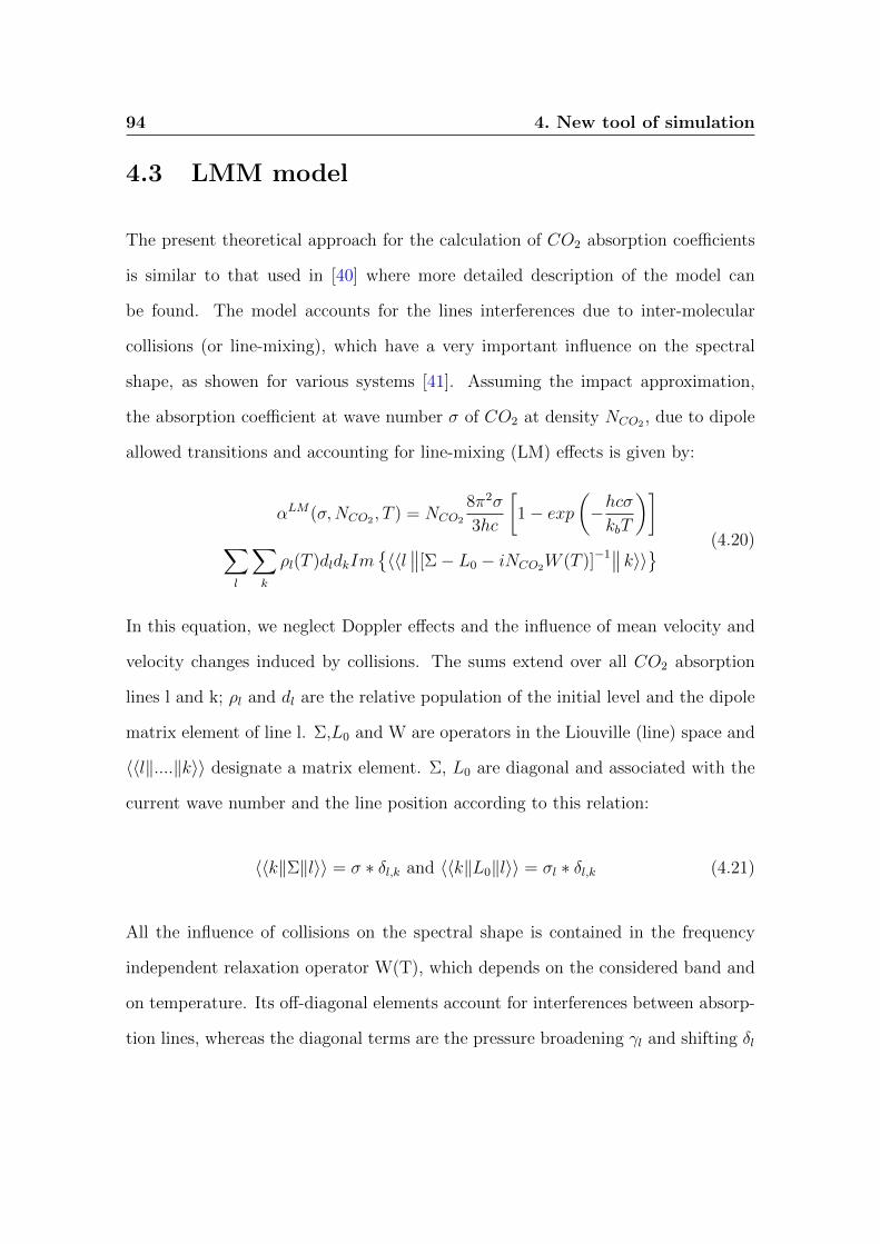
94 4. New tool of simulation
4.3 LMM model
The present theoretical approach for the calculation of CO2 absorption coefficients
is similar to that used in [40] where more detailed description of the model can
be found. The model accounts for the lines interferences due to inter-molecular
collisions (or line-mixing), which have a very important influence on the spectral
shape, as showen for various systems [41]. Assuming the impact approximation,
the absorption coefficient at wave number σ of CO2 at density NCO2 , due to dipole
allowed transitions and accounting for line-mixing (LM) effects is given by:
αLM(σ,NCO2 , T ) = NCO2
8π2σ
3hc
[1− exp
(−hcσkbT
)]∑l
∑k
ρl(T )dldkIm〈〈l∥∥[Σ− L0 − iNCO2W (T )]−1
∥∥ k〉〉 (4.20)
In this equation, we neglect Doppler effects and the influence of mean velocity and
velocity changes induced by collisions. The sums extend over all CO2 absorption
lines l and k; ρl and dl are the relative population of the initial level and the dipole
matrix element of line l. Σ,L0 and W are operators in the Liouville (line) space and
〈〈l‖....‖k〉〉 designate a matrix element. Σ, L0 are diagonal and associated with the
current wave number and the line position according to this relation:
〈〈k‖Σ‖l〉〉 = σ ∗ δl,k and 〈〈k‖L0‖l〉〉 = σl ∗ δl,k (4.21)
All the influence of collisions on the spectral shape is contained in the frequency
independent relaxation operator W(T), which depends on the considered band and
on temperature. Its off-diagonal elements account for interferences between absorp-
tion lines, whereas the diagonal terms are the pressure broadening γl and shifting δl

95
coefficients of isolates lines, i.e.:
〈〈l‖W (T )‖l〉〉 = γl(T )− iδl(T ) (4.22)
Recall that W satisfies two fundamental properties that are the detailed balance
principle:
〈〈k‖W (T )‖l〉〉 ∗ ρl(T ) = 〈〈l‖W (T )‖k〉〉 ∗ ρk(T ) (4.23)
and the sum rule:
∑l
dk〈〈k‖W (T )‖l〉〉 = 0 i.e∑k=l
dkdlRe〈〈k‖W (T )‖l〉〉 = −γl(T ) (4.24)
When line-mixing is neglected, W is diagonal and the usual sum of Lorentzian line
contributions is obtained as shown:
αNoLM(σ,NCO2 , T ) = N2CO2∗∑l
σ
σl
Sl(T )γl(T )π[σ − σl −NCO2δl(T )]2 + [NCO2γl(T )]
2
(4.25)
where Sl is the integrated intensity of line l and is given by:
Sl(T ) =8π3
3hcσl[1− exp(
−hcσlkbT
)]ρl(T )d2l (4.26)
4.3.1 Relaxation matrix
The model used in the present work to calculate the relaxation matrix W(T) is the
same than that used in previous works devoted to the CO2/air system [40] and [42]
where a detailed description of the model can be found. Within this approach, the
relaxation matrix is modelled by the energy corrected sudden scaling law, firstly

96 4. New tool of simulation
introduced by De Pristo and co-workers [43]. Note that line-mixing between lines of
different vibrational bands being very small, only interference between lines of the
same band is accounted for. The relaxation matrix element describing interference
between two lines of a given vibrational band is given by:
〈〈jijf‖W (T )‖j′ij′f〉〉 = (−1)l2i+l2f (2ji + 1)√
(2j′f + 1)(2jf + 1)
∑Leven
j′i L ji
l2i 0 −l2i
j′f L jf
−l2f 0 l2f
j′i j′f 1
jf j′f L
(2L+ 1)Ω(ji, T
Ω(L, T )Q(L, T )
(4.27)
In this expression, ji, jf and j′i, j′f are the rotational angular momentum quantum
number of the initial and final levels of the line l and k, respectively; l2 is the
vibrational angular quantum number. The element matrix inside ( ) and are 3J
and 6J coefficients [44]. Ω is the adiabacity factor, introduced into the model in
order to account for energy corrections and given by
Ω(j, T ) =
1 +
1
24
[ωj,j−2dcν(T )
]2−2
(4.28)
where ωj, j − 2, ν(T ) and dc are the frequency spacing between levels j and j-2, the
mean relative velocity in CO2-CO2 collisions and the scaling length. The rotational
cross sections (or the basic rates) Q(L,T) in eq.4.27 are modelled by the widely used
exponential power law
Q(L, T ) = A(T )[L(L+ 1)]−λ(T )exp
[−β(T )
hc ∗ ELkb ∗ T
](4.29)
97
In this equation, EL is the rotational energy of level L. The temperature (and per-
turbed) dependent quantities dc, A, λ, β are the parameters of the model. These
parameters can be deduced using the sum rule in equation 4.21 and through fits of
measured line-broadening coefficients.
4.3.2 Imaginary part of W
The imaginary part of the off-diagonal elements play a role at elevated pressure, as
shown in [45], [46]. Taking these imaginary elements into account in the calculation
does not significantly change the shape of the band but leads to opposite spectral
shifts of the P and R branches when line-mixing is very efficient. Imaginary off-
diagonal coupling terms within branches were thus added. They verify the detailed
balance principle, have opposite signs for R-R and P-P couplings and decrease with
the line separation. Their values were computed, for all bands at all pressures
and temperatures, from a single parameter which was adjusted from a high density
spectrum at the region of the 2ν1 + ν3 band.
4.3.3 Parameters needed to obtain absorption coefficients
The first data needed for the calculations are spectroscopic parameters of isolated
lines. Their identification, lower state energy, position, integrated intensity and self-
broadening coefficient were taken from the latest version of the HITRAN database
[1]. Note that for the temperatures, pressures and path lengths considered in the
present work, the use of the HITRAN database is sufficient. For higher temperatures
and longer path lengths, one may need to use a more adapted database, such as the
HITEMP database [2] and check the intensity cut-off criterion of the used database.

98 4. New tool of simulation
The temperature dependence of the self-broadening was assumed to be the same
as that of the air-broadening. This approximation is quite good when comparing
measured values in the 1.6 µm region for self- and air-broadened CO2 [6], [47]. For
the self- line-shifting coefficients, there is little data, except for measurements for
the 2ν1 + ν3, 3ν1 + ν3 and 3ν3 bands [6]-[48]. In order to build a line-shift data for
all bands, the approach of [49] has been used. The line-shifting coefficient of any
ro-vibrational line is thus written, as:
δ[(ν1 + ∆ν1, ν2 + ∆ν2, ν3 + ∆ν3, Jf )← (ν1, ν2ν3, Ji)] =
(Ji − Jf )δrot(|m|) + (a1∆ν1 + a2∆ν2 + a3∆ν3)δvib(|m|)(4.30)
where ν1, ν2, ν3 are the vibrational quantum numbers; ∆ν = ν ′−ν ′′ is the difference
of vibrational quantum numbers between the higher and lower states. The a1, a2,
a3 parameters and δrot(|m|), δvib(|m|) functions have been fitted to data measured
of the 2ν1+ν3, 3ν1+ν3 [50] and 3ν3 [51] bands, assuming that a1 = 2a2. Note that
the parameters of the present approach may be approximate since there are very
few data for the 3ν3 band [51]. New measurements of line shifts for pure CO2
are thus needed in order to improve the accuracy of the a1, a2, a3 parameters and
δrot(|m|), δvib(|m|) functions. The second set of data needed are the parameters for
the construction of the relaxation matrix W(T). Parameters dc, A, λ, β have been
determined using the sum rule 4.24. From these value, all off-diagonal elements
of the relaxation matrix have been computed using equations 4.27 and 4.29, while
the diagonal elements have been fixed to the values of the self -broadening. A re-
normalization procedure is then applied in order to satisfy the detailed balance and
the sum rule as described by [40].

Chapter 5
Results and Discussions
In this chapter the CO2 absorption coefficients measured at typical conditions of the
deep venusian atmosphere are shown. Comparisons between numerous measured
spectra and simulations calculated using three different models will be presented in
the second part of the chapter.
5.1 Experimental measurements
We recreate the same conditions found in the deep atmosphere of Venus as from the
Venus International Reference Atmosphere (VIRA) [52], which includes the tables
of the vertical structure of the venusian atmosphere. The VIRA model uses the
following inputs:
• new data on the chemical composition obtained from ground based and Galileo
observations of the near IR spectra of the Venus nightside emission. From
VEGA 1, 2 UV in situ spectrometry, Venera 15 infrared spectrometry; reanal-
ysis of Venera 11,13,14 spectrometry; Pioneer Venus entry probes and Orbiter

100 5. Results and Discussions
InfraRed sounding (OIR) data,
• vertical temperature and pressure profiles obtained from the VEGA 2 entry
probes, IR thermal sounding (Venera 15, Galileo), and from radio-occultation
(Venera 15,16, Pioneer Venus and Magellan Orbiters), horizontal T-profiles
from the VEGA 1,2 balloons,
• winds and turbulence measurements on the balloons, thermal winds retrieved
from T-profiles (Venera 15, Galileo);
• new data on the variability of the cloud structure (Venera 15 IR-spectrometry,
VEGA 1,2 entry probes and NIMS observations during the Galileo Venus fly-
by)
In order to reproduce the real vertical TP profile, we varied the pressure and
temperature of the CO2 from 1 to 30 bar and from 294 to 650 K respectively. This
corresponds to an altitude from about 50 km down to 15 km, as shown in figure 5.1.
Figure 5.1: Real vertical profile of the deep atmosphere of Venus used to obtain theCO2 absorption coefficients .
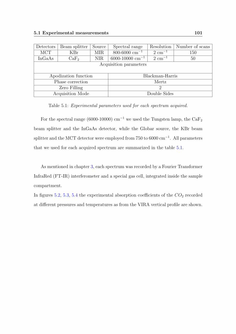
5.1 Experimental measurements 101
Detectors Beam splitter Source Spectral range Resolution Number of scansMCT KBr MIR 800-6000 cm−1 2 cm−1 150
InGaAs CaF2 NIR 6000-10000 cm−1 2 cm−1 50Acquisition parameters
Apodization function Blackman-HarrisPhase correction Mertz
Zero Filling 2Acquisition Mode Double Sides
Table 5.1: Experimental parameters used for each spectrum acquired.
For the spectral range (6000-10000) cm−1 we used the Tungsten lamp, the CaF2
beam splitter and the InGaAs detector, while the Globar source, the KBr beam
splitter and the MCT detector were employed from 750 to 6000 cm−1. All parameters
that we used for each acquired spectrum are summarized in the table 5.1.
As mentioned in chapter 3, each spectrum was recorded by a Fourier Transformer
InfraRed (FT-IR) interferometer and a special gas cell, integrated inside the sample
compartment.
In figures 5.2, 5.3, 5.4 the experimental absorption coefficients of the CO2 recorded
at different pressures and temperatures as from the VIRA vertical profile are shown.

102 5. Results and Discussions
Figure 5.2: CO2 absorption coefficients at different pressures and temperatures.These physical conditions correspond to an altitude of 32 km down to 22 km.
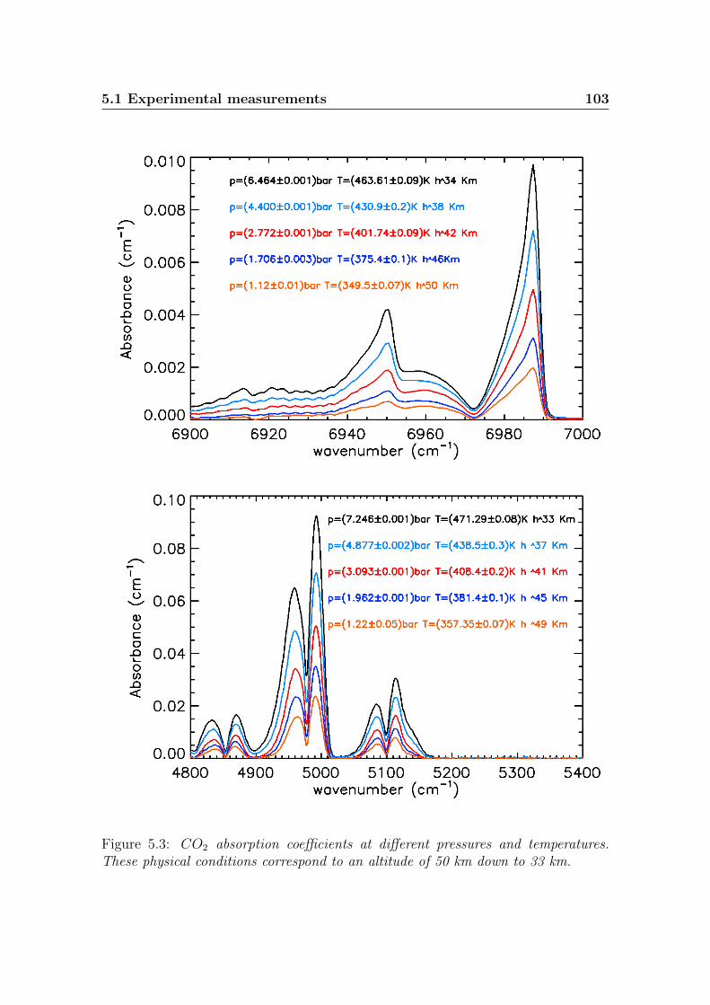
5.1 Experimental measurements 103
Figure 5.3: CO2 absorption coefficients at different pressures and temperatures.These physical conditions correspond to an altitude of 50 km down to 33 km.
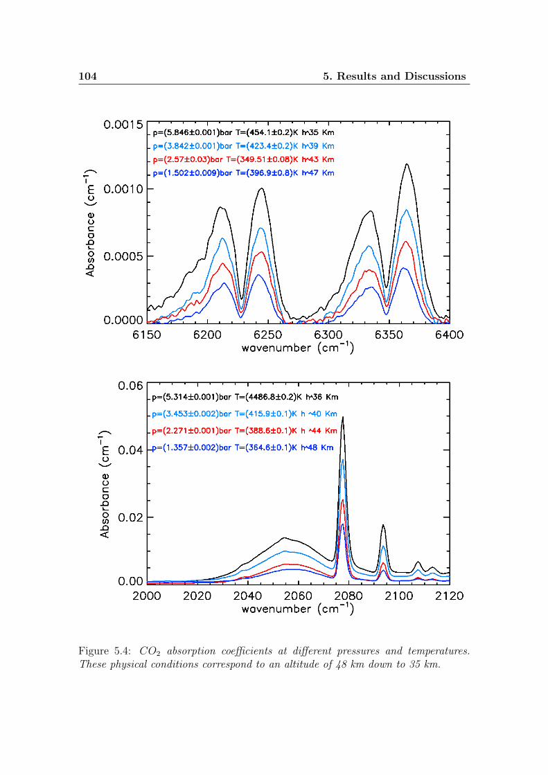
104 5. Results and Discussions
Figure 5.4: CO2 absorption coefficients at different pressures and temperatures.These physical conditions correspond to an altitude of 48 km down to 35 km.
5.1 Experimental measurements 105
For low pressures (see figure 5.3) and low temperature, we can distinguish the
roto-vibrational structures, in the spectral range range [6850-7000] cm−1. These
vanish when we increase the pressure, because the collision line width increases
with the density as the mean time between collisions decreases. It is due to the
modification of molecular potentials, and hence to the energy levels, which take
place during each emission or absorption process, and is caused by inelastic as well
as elastic collisions between the molecule and the surrounding ones.
In first approximation, the shape of the line is still Lorentzian and the width is
proportional to the pressure. In order to quantify this behavior, we have calculated
the band integrated area in different spectral regions, and have plotted this values
toward the pressure. As shown in figure 5.5, we obtain a linear fit (red curve) with
residual fit better than 99%. In figure 5.5 (on bottom) we reported also a polynomial
fit, because in this spectral range, the broadening of the CO2 bands is due to the
combined contribution of the pressure and Collision Induced Absorption (CIA), a
phenomenon that will be described with more details in the section 5.3.
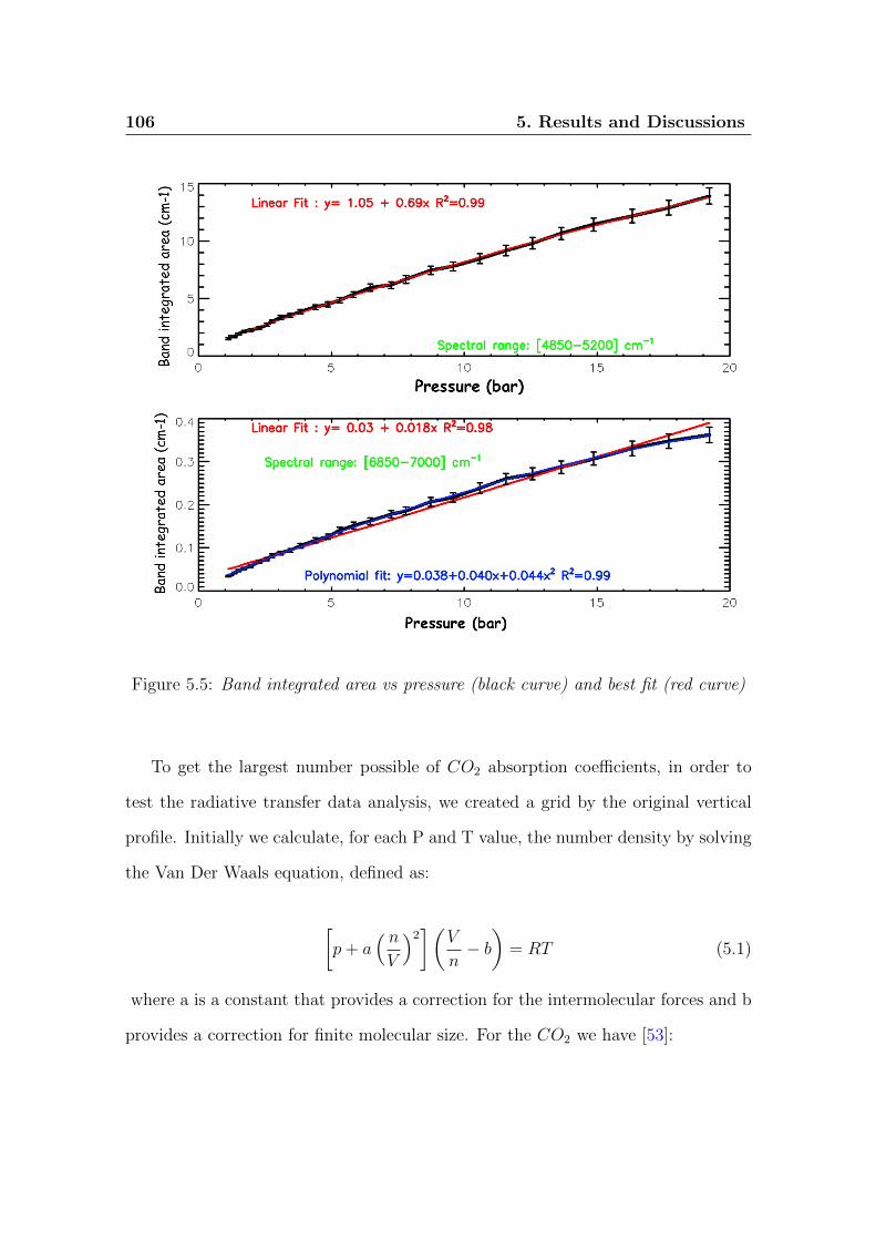
106 5. Results and Discussions
Figure 5.5: Band integrated area vs pressure (black curve) and best fit (red curve)
To get the largest number possible of CO2 absorption coefficients, in order to
test the radiative transfer data analysis, we created a grid by the original vertical
profile. Initially we calculate, for each P and T value, the number density by solving
the Van Der Waals equation, defined as:
[p+ a
( nV
)2](
V
n− b)
= RT (5.1)
where a is a constant that provides a correction for the intermolecular forces and b
provides a correction for finite molecular size. For the CO2 we have [53]:

5.1 Experimental measurements 107
a= 3.96*10−1 (Pa m 3)
b= 42.69*10−6 (m3mol−1)
Increasing and decreasing of 30C the initial values of temperatures, maintaining
the density of the CO2 constant, we deduced in according to the equation 5.1, the
new value of the pressures. In this way, we obtain two new ”profiles” of temperature
and pressure, as shown in the figure 5.6.
Figure 5.6: The three profile along we recorded the CO2 absorption coefficients. Theblack curve is the real vertical profile, the blue is obtained decreasing the T of 30Cand the red is obtained increasing the T of 30C.
For each point of this grid, we obtained the CO2 absorption coefficients, acquired
in the spectral range from 700 to 10000 cm−1 and with the same experimental
parameters, i.e resolution 2 cm−1, number scans 150.
108 5. Results and Discussions
Measurements errors
There are two potential sources for photometric error in Fourier Transformer In-
fraRed interferometer: one is due to the linearity and the second one to the ”single
beam”.
The first one and most critical source of photometric error is the non-linear photo-
metric response of the detector and possibly its associated electronics. This effect
may occur as a distortion of the spectrum, but in our case we have never encoun-
tered such anomaly. Therefore we can say that this source of error can be neglected.
The single beam is only a problem if there is a significant change in the system’s
response in the time frame from the acquisition of a reference to a sample spectrum.
This might be due to drifts in the lamp used as source or change in the transmittance
of the optical path due to atmospheric water vapour or carbon dioxide. Recording
the reference spectrum at the same environmental conditions of the sample, is very
important in order to remove, as much as possible, the contribution of the water
vapour and CO2, present along the optical path of the FT-IR off the cell. However,
even small variation of the air conditions within the optical path translate into a not
perfect compensation and consequently it’s seen as a residual in the transmittance
affecting the uncertainty. A way to reduce this error is a much as possible, is reduce
the time interval between the reference and sample acquisition. For what has been
said, we can assert that our measurements are affect by errors due to the drift of the
system (lamps, air, detector etc). Therefore, in order to evaluate the uncertainty,
we have recorded 10 CO2 transmittances under the same conditions, calculated the
average value, <Transmittance>, and its standard deviation σ. In all cases of in-
terest, we have that the σT=2% of the spectral range. To obtain the final errors,

5.1 Experimental measurements 109
we must remember that the figures show the CO2 absorption coefficients (see for
example the figure 5.2); therefore, referring to the equation 3.2.2, and applying the
propagation statistical errors rule, we have:
σ(Absorbance) =
√(∂Absorbance
∂T
)2
σ2T +
(∂Absorbance
∂l
)2
σ2l (5.2)
The σl is not a statistical error but a measurement error. In figure 5.7, an example
of the error calculated applying the equation 5.1is shown. In the bottom panel, we
reported only the errors without absorption coefficients to show the entity of the
errors.
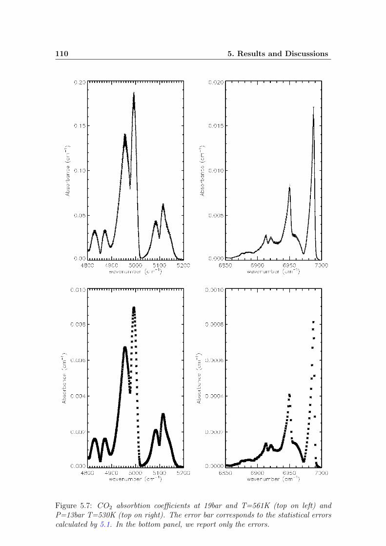
110 5. Results and Discussions
Figure 5.7: CO2 absorbtion coefficients at 19bar and T=561K (top on left) andP=13bar T=530K (top on right). The error bar corresponds to the statistical errorscalculated by 5.1. In the bottom panel, we report only the errors.

5.2 Comparison between simulated and measured data 111
5.2 Comparison between simulated and measured
data
The measurements have been compared with synthetic spectra obtained from the
three different models described in chapter 4. The figure 5.8 shows results obtained
for the 3ν1+ν3 tetrad region at room temperature and 20bar.
Figure 5.8: Comparison between measured (red curve) and simulated spectra of CO2
at room temperature and 20 bar. The black curve is obtained by LMM, the greenand blue curves are obtained by Solution and by ARS code respectively.
These results confirm that Lorentz line shapes are not a good approximation at
high pressure and it’s necessary take into account the line mixing effect. In fact, as
you can see in figure, the blue curve, obtained by ARS code which neglects this effect,

112 5. Results and Discussions
underestimates the absorption in the central part of the band. The same behavior is
obtained with Solution code (green curve), which considers the line mixing effect but
its models the line shape according to figure 4.1. The differences between spectra
simulated using the three different models and measured increase with pressure and
temperature, as you can see in figure 5.9.
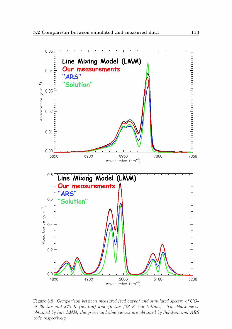
5.2 Comparison between simulated and measured data 113
Figure 5.9: Comparison between measured (red curve) and simulated spectra of CO2
at 20 bar and 373 K (on top) and 40 bar 473 K (on bottom). The black curveobtained by line LMM, the green and blue curves are obtained by Solution and ARScode respectively.

114 5. Results and Discussions
In order to quantify the matching between simulated and measured spectra,
we calculated the integrated band area in different spectral range and evaluated the
difference between experimental and synthetic spectra. We have chosen this method
in order to estimate the goodness of the models, because it allows us to evaluate with
greater accuracy also the less intense absorptions. Moreover, as shown in figure, we
can select every range of interest carefully.
Figure 5.10: Example of the band integrated area method. A straight line is drawnbetween the two frequency limits and the area is calculated.

5.2 Comparison between simulated and measured data 115
Results are reported in table 5.2. As you can see we have the match fit with the
”LMM” on all the measured spectral ranges, in fact differences between our data
and synthetic spectra are smaller respect to the other models.
∆(M−LMM)LMM
∆(M−Sol)Sol
∆(M−ARS)ARS
Spectral Range p (bar)cm−1 T (K)
0.03 0.3 0.08 2115-2025 10 bar 294 K0.004 0.4 0.2 7050-6880 20 bar 294 K0.02 0.6 0.5 8350-8150 40 bar 294 K
9.2*10−4 0.1 0.2 4800-5200 40bar 373 K0.06 0.3 0.3 6100-6500 40 bar 373 K0.002 0.3 0.2 6850-7050 40 bar 373 K
Table 5.2: Difference between integrated band area of the experimental and simulatedspectra. M refer to the ”measurements”, LMM, Sol and ARS refer to ”Line MixingModel”, Solution and ARS Code respectively.
These results lead us to conclude that for gases under extreme conditions, the
shape of the spectral lines no longer follows the conventional Lorentzian form and
that it is mandatory to take into account the line mixing effect to reduce the dis-
crepancy.
In the remainder of this chapter, we will then report only the results obtained using
the mixing-line model, analyzing the far wings region. This part of the spectrum is
very important to improve the remote sensing data analysis for better interpreter
the data coming from the space missions, in particular from VIRTIS instrument on
board of Venus Express mission.
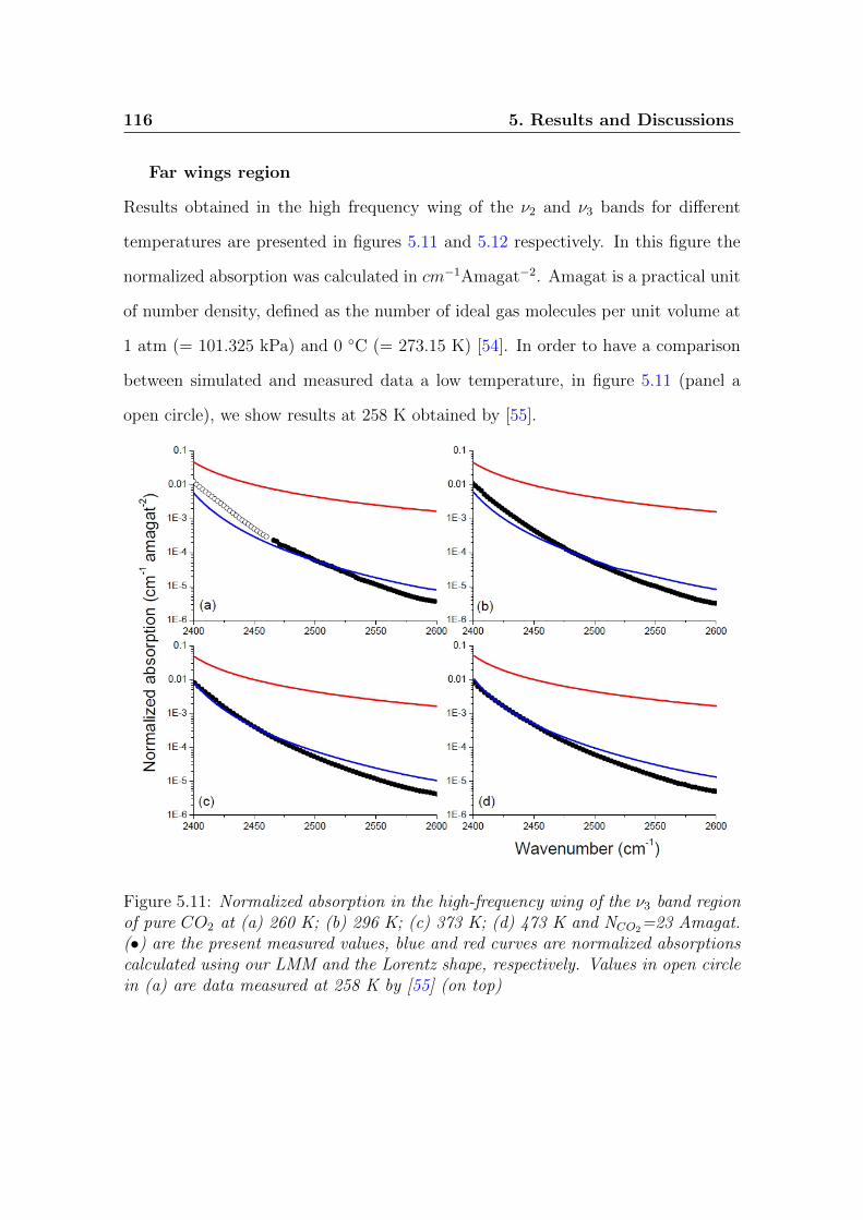
116 5. Results and Discussions
Far wings region
Results obtained in the high frequency wing of the ν2 and ν3 bands for different
temperatures are presented in figures 5.11 and 5.12 respectively. In this figure the
normalized absorption was calculated in cm−1Amagat−2. Amagat is a practical unit
of number density, defined as the number of ideal gas molecules per unit volume at
1 atm (= 101.325 kPa) and 0 C (= 273.15 K) [54]. In order to have a comparison
between simulated and measured data a low temperature, in figure 5.11 (panel a
open circle), we show results at 258 K obtained by [55].
Figure 5.11: Normalized absorption in the high-frequency wing of the ν3 band regionof pure CO2 at (a) 260 K; (b) 296 K; (c) 373 K; (d) 473 K and NCO2=23 Amagat.(•) are the present measured values, blue and red curves are normalized absorptionscalculated using our LMM and the Lorentz shape, respectively. Values in open circlein (a) are data measured at 258 K by [55] (on top)
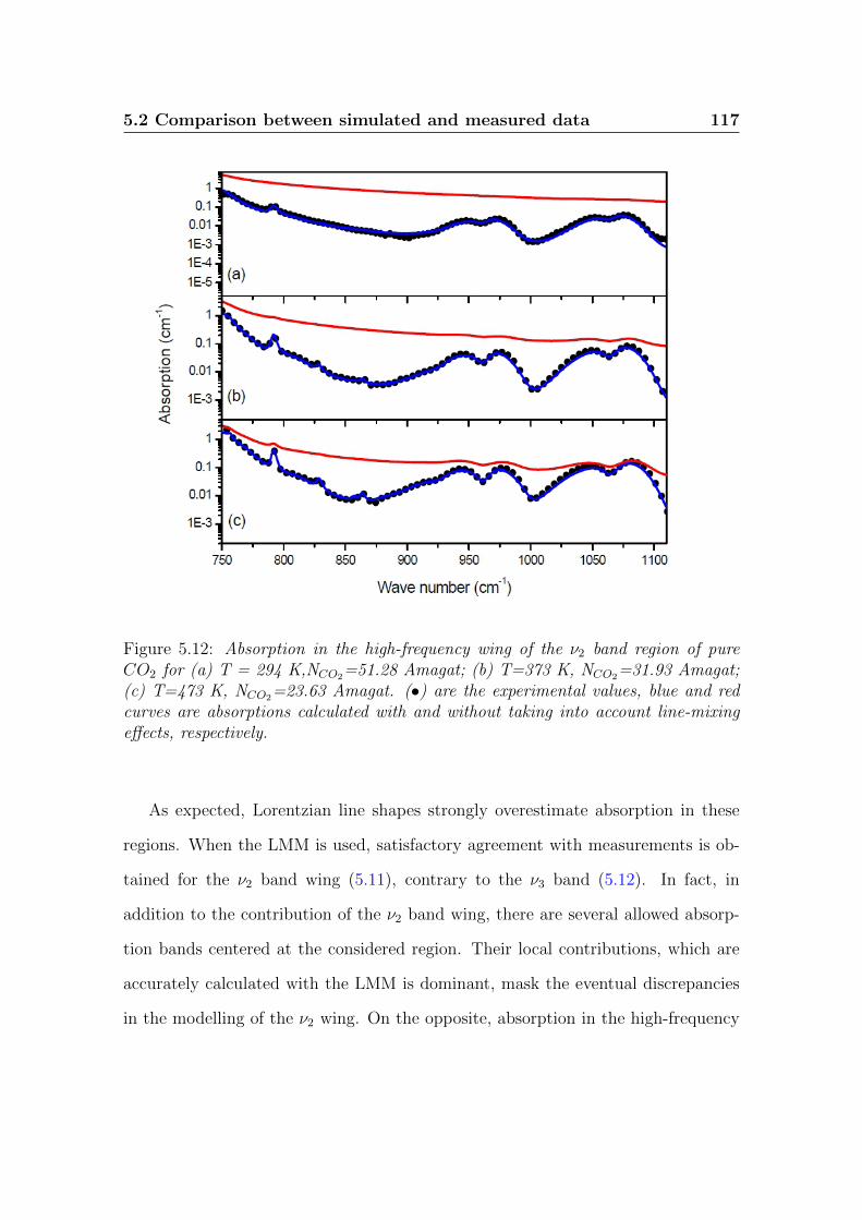
5.2 Comparison between simulated and measured data 117
Figure 5.12: Absorption in the high-frequency wing of the ν2 band region of pureCO2 for (a) T = 294 K,NCO2=51.28 Amagat; (b) T=373 K, NCO2=31.93 Amagat;(c) T=473 K, NCO2=23.63 Amagat. (•) are the experimental values, blue and redcurves are absorptions calculated with and without taking into account line-mixingeffects, respectively.
As expected, Lorentzian line shapes strongly overestimate absorption in these
regions. When the LMM is used, satisfactory agreement with measurements is ob-
tained for the ν2 band wing (5.11), contrary to the ν3 band (5.12). In fact, in
addition to the contribution of the ν2 band wing, there are several allowed absorp-
tion bands centered at the considered region. Their local contributions, which are
accurately calculated with the LMM is dominant, mask the eventual discrepancies
in the modelling of the ν2 wing. On the opposite, absorption in the high-frequency

118 5. Results and Discussions
side of the ν3 band is almost entirely due to far wing of this band lines for which the
impact approach breaks down. Similar results are obtained for the high-frequency
wings of the ν1+ν3 and 2ν1+ν3 bands.
For an accurate description of far wing contributions, the widely used empirical
correction to the Lorentz line shape has thus been used. Within this approach, the
absorption for pure CO2 is expressed by:
αwing(σ,NCO2 , T ) = NCO2
∑l
exp
[h
(σ − σl2KBT
]σ
σl∗
Sl(T )γl(T )
π[σ − σl −NCO2δl(T )]2 + [NCO2γl(T )]2∗ χ(T, |σ − σl|)
(5.3)
The line shape correction factor χ is assumed independent of the transition. The
exponential term in equation 5.3 is due to the initial correlations and results in an
asymmetry of the far wing [56], [57]. A set of χ factors for pure CO2 in the ν3 band
head region and for a wide range of temperature [220-750 K] was constructed in [58].
In [59] the high-frequency wings of the ν3, ν1+ν3 and 3ν3 bands were investigated
at 296 and 431 K. Apart from these studies, most others are devoted to the ν3 band
and/or for room temperature. Note that, to our knowledge, no data are available
for the ν2 band wing despite its importance. In this work, three new sets of χ factors
have been constructed for the ν2, ν3 and ν1+ν3 band wings by fitting measured data
at different temperature through using equation 5.3.
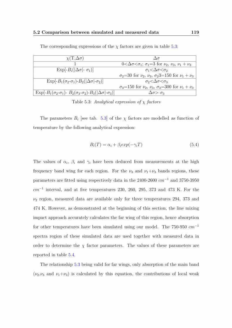
5.2 Comparison between simulated and measured data 119
The corresponding expressions of the χ factors are given in table 5.3:
χ(T,∆σ) ∆σ1 0<∆σ<σ1; σ1=3 for ν2, ν3, ν1 + ν3
Exp[-Bi(|∆σ|- σ1)] σ1<∆σ<σ2
σ2=30 for ν2, ν3, σ23=150 for ν1 + ν3
Exp[-B1(σ2-σ1)-B2(|∆σ|-σ2)] σ2<∆σ<σ3
σ3=150 for ν2, ν3, σ3=300 for ν1 + ν3
Exp[-B1(σ2-σ1)- B2(σ3-σ2)-B3(|∆σ|-σ3)] ∆σ> σ3
Table 5.3: Analytical expression of χ factors
The parameters Bi [see tab. 5.3] of the χ factors are modelled as function of
temperature by the following analytical expression:
Bi(T ) = αi + βiexp(−γiT ) (5.4)
The values of αi, βi and γi have been deduced from measurements at the high
frequency band wing for each region. For the ν3 and ν1+ν3 bands regions, these
parameters are fitted using respectively data in the 2400-2600 cm−1 and 3750-3950
cm−1 interval, and at five temperatures 230, 260, 295, 373 and 473 K. For the
ν2 region, measured data are available only for three temperatures 294, 373 and
474 K. However, as demonstrated at the beginning of this section, the line mixing
impact approach accurately calculates the far wing of this region, hence absorption
for other temperatures have been simulated using our model. The 750-950 cm−1
spectra region of these simulated data are used together with measured data in
order to determine the χ factor parameters. The values of these parameters are
reported in table 5.4.
The relationship 5.3 being valid for far wings, only absorption of the main band
(ν2,ν3 and ν1+ν3) is calculated by this equation, the contributions of local weak

120 5. Results and Discussions
ν2 Band ν3 Band ν1 + ν3 Bandα β γ α β γ α β γ
B1 0.1034 1.962 0.0203 0.0727 -0.3830 0.0105 0.03 -0.3507 0.01804B2 0.0145 0 0 0.0229 0.1355 0.0109 0.0156 2174.3 0.0575B3 0.0099 0 0 0.0231 0 0 0.0082 0 0
Table 5.4: Values of the χ factors parameters deduced from experiments.
bands are calculated using the LMM as described in the section 4.3. A comparison
between measured and calculated values for the ν3 band wings regions is presented
in figure 5.13 at 295 K and 473 K.
Figure 5.13: Pure CO2 normalized absorption coefficients at the ν3 band wing re-gions for T = 295 K (top); T = 473 K (bottom) and NCO2=17.6 Amagat. (•) andgreen curve are respectively measured and calculated values. Measured data at roomtemperature (top) of previous studies are also reported for comparison: the red dottedcurve are values of [60] in the left and [55] in the right, the green dotted curve arevalues from [58]
Note that accounting for the initial correlation [exponential term in equation 5.3]
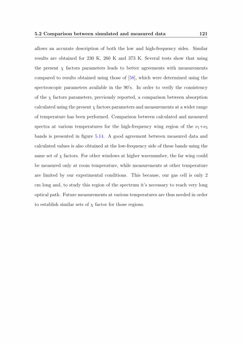
5.2 Comparison between simulated and measured data 121
allows an accurate description of both the low and high-frequency sides. Similar
results are obtained for 230 K, 260 K and 373 K. Several tests show that using
the present χ factors parameters leads to better agreements with measurements
compared to results obtained using those of [58], which were determined using the
spectroscopic parameters available in the 90’s. In order to verify the consistency
of the χ factors parameters, previously reported, a comparison between absorption
calculated using the present χ factors parameters and measurements at a wider range
of temperature has been performed. Comparison between calculated and measured
spectra at various temperatures for the high-frequency wing region of the ν1+ν3
bands is presented in figure 5.14. A good agreement between measured data and
calculated values is also obtained at the low-frequency side of these bands using the
same set of χ factors. For other windows at higher wavenumber, the far wing could
be measured only at room temperature, while measurements at other temperature
are limited by our experimental conditions. This because, our gas cell is only 2
cm long and, to study this region of the spectrum it’s necessary to reach very long
optical path. Future measurements at various temperatures are thus needed in order
to establish similar sets of χ factor for those regions.
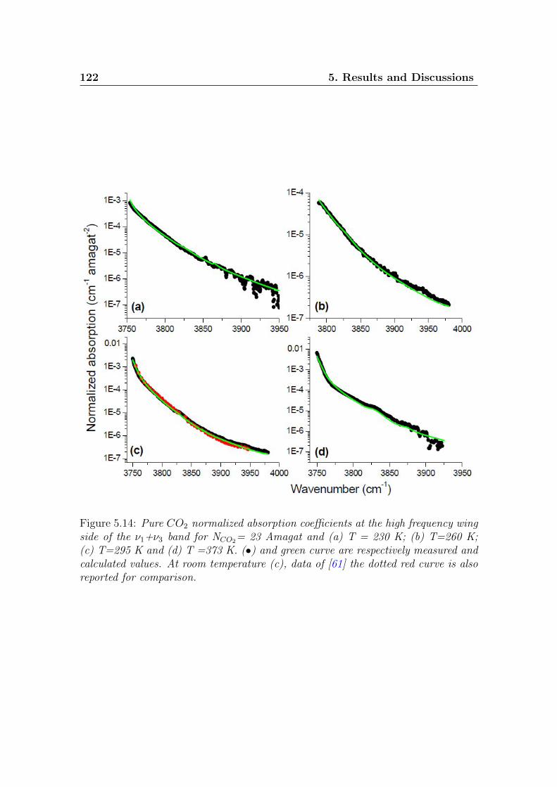
122 5. Results and Discussions
Figure 5.14: Pure CO2 normalized absorption coefficients at the high frequency wingside of the ν1+ν3 band for NCO2= 23 Amagat and (a) T = 230 K; (b) T=260 K;(c) T=295 K and (d) T =373 K. (•) and green curve are respectively measured andcalculated values. At room temperature (c), data of [61] the dotted red curve is alsoreported for comparison.

5.2 Comparison between simulated and measured data 123
After an extensive discussion on the very good results obtained with the LMM,
in figures 5.15, we show some comparison between our experimental data, measured
as a from the VIRA profile and synthetic spectra obtained with this model. As you
can see, the two curves superposed in all spectral range and at very different physical
conditions. Also in this case, to test the goodness of the best fit between simulated
and measured data, we calculated the band integrated area and the difference. As
you can see in table 5.5, we have a matching better than 98% for most cases of
interest.
Errors indicated in table 5.5 are statistical errors evaluated as standard deviation of
the fluctuation of the pressure and temperature values during the acquisition of the
spectra.
The values indicated with ∗ refer to the comparison shown in figure 5.15.

124 5. Results and Discussions
Figure 5.15: Comparison between measured (red curve) and simulated (black curve)data by LMM.
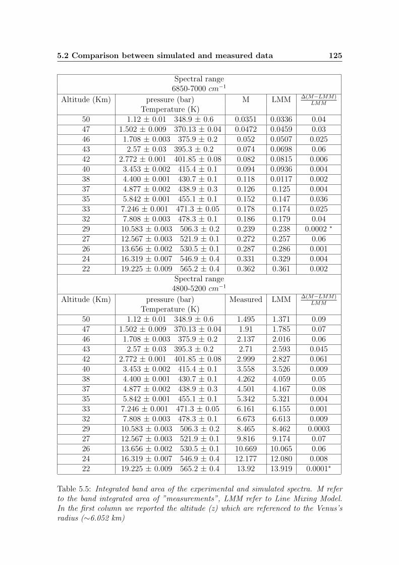
5.2 Comparison between simulated and measured data 125
Spectral range6850-7000 cm−1
Altitude (Km) pressure (bar) M LMM ∆(M−LMM)LMM
Temperature (K)50 1.12 ± 0.01 348.9 ± 0.6 0.0351 0.0336 0.0447 1.502 ± 0.009 370.13 ± 0.04 0.0472 0.0459 0.0346 1.708 ± 0.003 375.9 ± 0.2 0.052 0.0507 0.02543 2.57 ± 0.03 395.3 ± 0.2 0.074 0.0698 0.0642 2.772 ± 0.001 401.85 ± 0.08 0.082 0.0815 0.00640 3.453 ± 0.002 415.4 ± 0.1 0.094 0.0936 0.00438 4.400 ± 0.001 430.7 ± 0.1 0.118 0.0117 0.00237 4.877 ± 0.002 438.9 ± 0.3 0.126 0.125 0.00435 5.842 ± 0.001 455.1 ± 0.1 0.152 0.147 0.03633 7.246 ± 0.001 471.3 ± 0.05 0.178 0.174 0.02532 7.808 ± 0.003 478.3 ± 0.1 0.186 0.179 0.0429 10.583 ± 0.003 506.3 ± 0.2 0.239 0.238 0.0002 ∗
27 12.567 ± 0.003 521.9 ± 0.1 0.272 0.257 0.0626 13.656 ± 0.002 530.5 ± 0.1 0.287 0.286 0.00124 16.319 ± 0.007 546.9 ± 0.4 0.331 0.329 0.00422 19.225 ± 0.009 565.2 ± 0.4 0.362 0.361 0.002
Spectral range4800-5200 cm−1
Altitude (Km) pressure (bar) Measured LMM ∆(M−LMM)LMM
Temperature (K)50 1.12 ± 0.01 348.9 ± 0.6 1.495 1.371 0.0947 1.502 ± 0.009 370.13 ± 0.04 1.91 1.785 0.0746 1.708 ± 0.003 375.9 ± 0.2 2.137 2.016 0.0643 2.57 ± 0.03 395.3 ± 0.2 2.71 2.593 0.04542 2.772 ± 0.001 401.85 ± 0.08 2.999 2.827 0.06140 3.453 ± 0.002 415.4 ± 0.1 3.558 3.526 0.00938 4.400 ± 0.001 430.7 ± 0.1 4.262 4.059 0.0537 4.877 ± 0.002 438.9 ± 0.3 4.501 4.167 0.0835 5.842 ± 0.001 455.1 ± 0.1 5.342 5.321 0.00433 7.246 ± 0.001 471.3 ± 0.05 6.161 6.155 0.00132 7.808 ± 0.003 478.3 ± 0.1 6.673 6.613 0.00929 10.583 ± 0.003 506.3 ± 0.2 8.465 8.462 0.000327 12.567 ± 0.003 521.9 ± 0.1 9.816 9.174 0.0726 13.656 ± 0.002 530.5 ± 0.1 10.669 10.065 0.0624 16.319 ± 0.007 546.9 ± 0.4 12.177 12.080 0.00822 19.225 ± 0.009 565.2 ± 0.4 13.92 13.919 0.0001∗
Table 5.5: Integrated band area of the experimental and simulated spectra. M referto the band integrated area of ”measurements”, LMM refer to Line Mixing Model.In the first column we reported the altitude (z) which are referenced to the Venus’sradius (∼6.052 km)
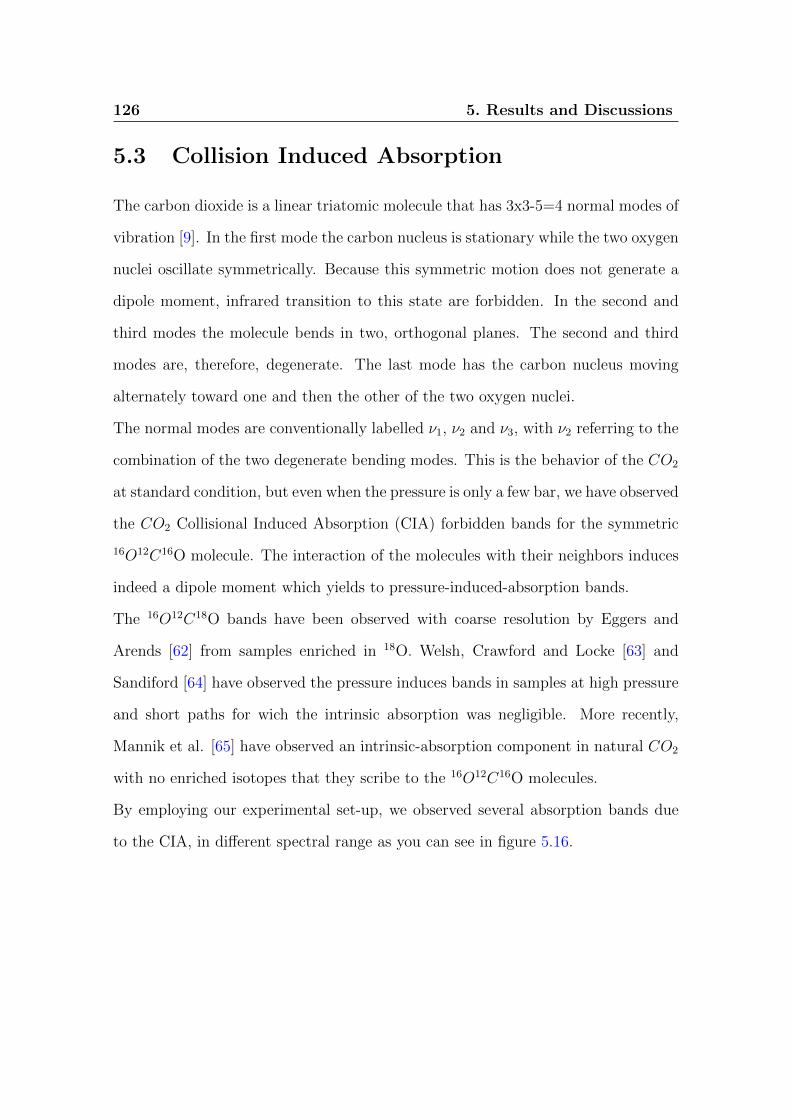
126 5. Results and Discussions
5.3 Collision Induced Absorption
The carbon dioxide is a linear triatomic molecule that has 3x3-5=4 normal modes of
vibration [9]. In the first mode the carbon nucleus is stationary while the two oxygen
nuclei oscillate symmetrically. Because this symmetric motion does not generate a
dipole moment, infrared transition to this state are forbidden. In the second and
third modes the molecule bends in two, orthogonal planes. The second and third
modes are, therefore, degenerate. The last mode has the carbon nucleus moving
alternately toward one and then the other of the two oxygen nuclei.
The normal modes are conventionally labelled ν1, ν2 and ν3, with ν2 referring to the
combination of the two degenerate bending modes. This is the behavior of the CO2
at standard condition, but even when the pressure is only a few bar, we have observed
the CO2 Collisional Induced Absorption (CIA) forbidden bands for the symmetric
16O12C16O molecule. The interaction of the molecules with their neighbors induces
indeed a dipole moment which yields to pressure-induced-absorption bands.
The 16O12C18O bands have been observed with coarse resolution by Eggers and
Arends [62] from samples enriched in 18O. Welsh, Crawford and Locke [63] and
Sandiford [64] have observed the pressure induces bands in samples at high pressure
and short paths for wich the intrinsic absorption was negligible. More recently,
Mannik et al. [65] have observed an intrinsic-absorption component in natural CO2
with no enriched isotopes that they scribe to the 16O12C16O molecules.
By employing our experimental set-up, we observed several absorption bands due
to the CIA, in different spectral range as you can see in figure 5.16.
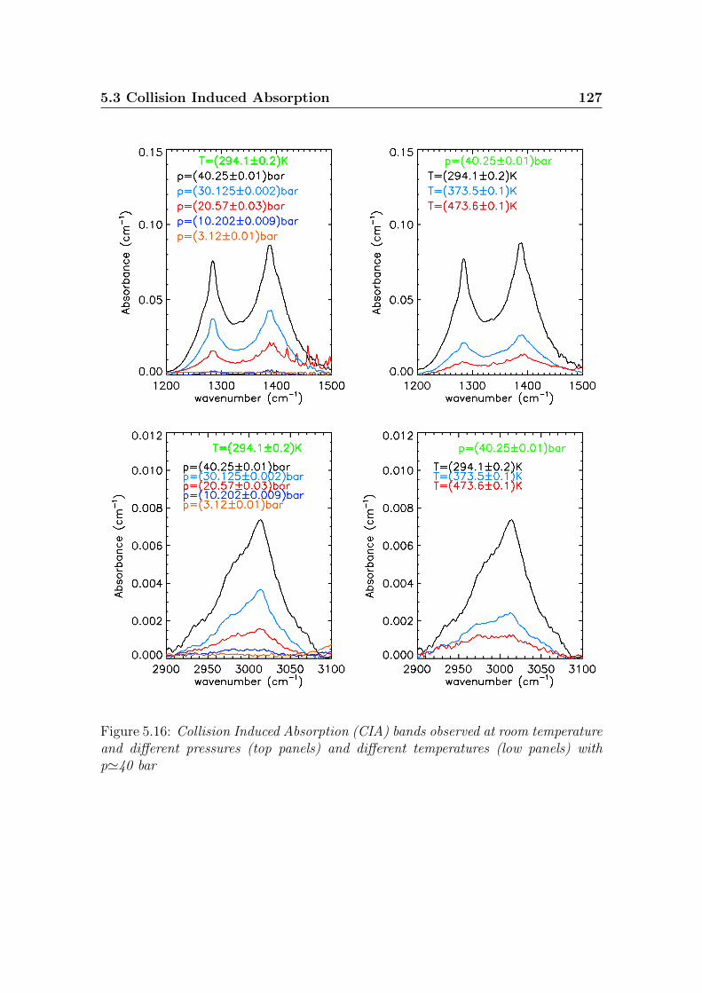
5.3 Collision Induced Absorption 127
Figure 5.16: Collision Induced Absorption (CIA) bands observed at room temperatureand different pressures (top panels) and different temperatures (low panels) withp'40 bar
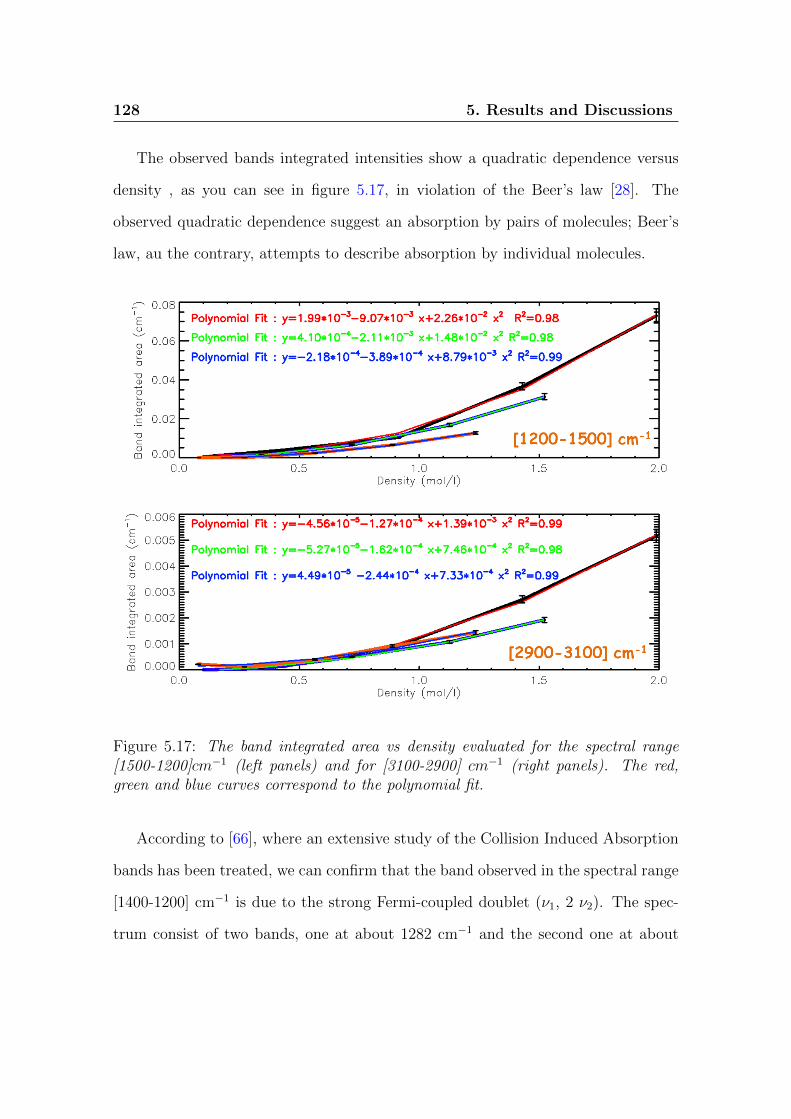
128 5. Results and Discussions
The observed bands integrated intensities show a quadratic dependence versus
density , as you can see in figure 5.17, in violation of the Beer’s law [28]. The
observed quadratic dependence suggest an absorption by pairs of molecules; Beer’s
law, au the contrary, attempts to describe absorption by individual molecules.
Figure 5.17: The band integrated area vs density evaluated for the spectral range[1500-1200]cm−1 (left panels) and for [3100-2900] cm−1 (right panels). The red,green and blue curves correspond to the polynomial fit.
According to [66], where an extensive study of the Collision Induced Absorption
bands has been treated, we can confirm that the band observed in the spectral range
[1400-1200] cm−1 is due to the strong Fermi-coupled doublet (ν1, 2 ν2). The spec-
trum consist of two bands, one at about 1282 cm−1 and the second one at about
5.3 Collision Induced Absorption 129
1390 cm−1. These bands represent the pronounced Q branches surrounded by P- and
R-like branches. Interestingly, the peak intensities of R- exceed those of P branches.
This result is comparable with that found in [67] by high-resolution CARS probings
in free expanding jet. This work assigned definitely a peak at 1284.73 cm−1 to car-
bon dioxide dimer.
The peak intensity increases with the pressure, as shown in figure 5.16 (on left),
and decrease with the temperature. This is probably due to the dissociation energy
of dimers, determined in [68] as the thermally excited state-selected energy statisti-
cally averaged over an ensemble of quansidiatomic molecules at equilibrium. Under
harmonic oscillator approximation, the effective dissociation energy is expressed by:
〈D0〉 = D0 − 2T1−
[1 + D0
T+ 1
2
(D0
T
)2]exp
(−D0
T
)1−
(1 + D0
T
)exp
(−D0
T
) (5.5)
where D0 is expressed in K. You can note that the terminal value of the thermally av-
eraged dissociation energy at T→∞ is equal to D0/3. The intermolecular potential
well depth for the (CO2)2 dimer is about 700K. Presupposing four intermolecular
vibrations to have a mean frequency about ν=35 cm−1, the zero point vibrational
energy can be estimated to be of the order of 100K. Hence, the dissociation energy
of (CO2)2 dimer is about D0=600K.
It should be noted that the absorption by CO2 is relatively weak (0.10 cm−1 or less
at 40 bar, as shown in figure 5.16) throughout the 1100-1835 cm−1 region and has
not been studied as in the other part of the electromagnetic spectrum. The CO2
absorption is negligible in the earth’s atmosphere except for very long optical paths,
but plays an important role in the radiative transfer in atmospheres of planets such
as Venus that contain vast amounts of CO2 (about 96 %).
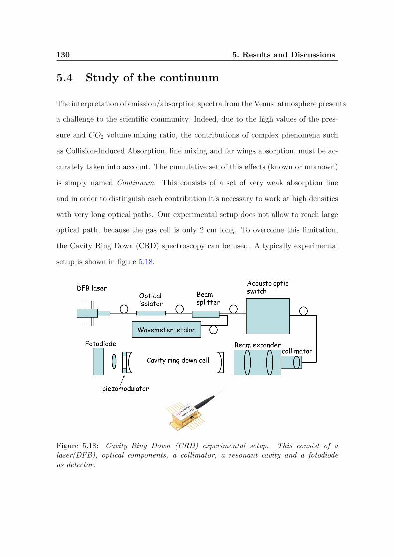
130 5. Results and Discussions
5.4 Study of the continuum
The interpretation of emission/absorption spectra from the Venus’ atmosphere presents
a challenge to the scientific community. Indeed, due to the high values of the pres-
sure and CO2 volume mixing ratio, the contributions of complex phenomena such
as Collision-Induced Absorption, line mixing and far wings absorption, must be ac-
curately taken into account. The cumulative set of this effects (known or unknown)
is simply named Continuum. This consists of a set of very weak absorption line
and in order to distinguish each contribution it’s necessary to work at high densities
with very long optical paths. Our experimental setup does not allow to reach large
optical path, because the gas cell is only 2 cm long. To overcome this limitation,
the Cavity Ring Down (CRD) spectroscopy can be used. A typically experimental
setup is shown in figure 5.18.
Figure 5.18: Cavity Ring Down (CRD) experimental setup. This consist of alaser(DFB), optical components, a collimator, a resonant cavity and a fotodiodeas detector.
5.4 Study of the continuum 131
It’s consists of a laser that is used to illuminate a stable optical cavity, formed by
two highly reflecting plano-concave mirrors. The laser is used as a source, because is
monochromatic, extremely bright and both spatially and temporally coherent. The
fraction of light entering the cavity on one side ‘rings’ back and forth many times
between the two mirrors. The time behavior of the light intensity inside the cavity
ICRD(t), can be monitored by the small fraction of light that is transmitted through
the other mirror.
If the only loss factor in the cavity is the reflectivity loss of the mirrors, one can
show that the light intensity inside the cavity decays exponentially in time with a
decay constant τ , the ring down time, given by:
τ =d
c(|lnR|). (5.6)
Here d is the optical path length between the mirrors, c is the speed of light and R
is the reflectivity of the mirrors.
If there is additional loss inside the cavity due to the presence of absorber such
as CO2, the light intensity inside the cavity will still decay exponentially in time
provided the absorption follows Beer’s law. One can be shown that the product of
the frequency dependent absorption cross-section with the number density Ni(x) is
commonly expressed as the absorption coefficient ki(ν, x). For a detailed description
refer to [69]. Thanks to this technique, we can analyze also the less abundant iso-
topic carbon dioxide species, temperature dependence of absorption and broadening
parameters, as well as different phenomena such as Collision Induced Absorption.
Although this technique has many advantages, it also has many restrictions. One
in particular is due to the narrow range in which lasers operate. In fact, although
132 5. Results and Discussions
tunable, this source may cover up to 100nm as a maximum. In order to characterize
the optical properties of gases in a wide spectral range, several lasers are needed
and are often very expensive. In addition to that, many cavities are also needed
because, the mirrors used, cannot be adapted throughout in all spectral ranges of
interest.
For the current study, we used a FT-IR to cover a wide spectral range in order to
test the tools of simulation
Conclusions
In this thesis we presented a new experimental setup able to characterize the optical
properties of gases at typically planetary conditions, in particular high pressure and
high temperature. We prefixed two scientific objectives: to measure CO2 absorp-
tion coefficients in order to expand the available spectroscopic databases to better
match the broadening and line mixing effect; to update the commonly used tools
of radiative transfer calculation in order to improve the accuracy of remote sensing
data analysis. In light of the results presented in this work, many experimental data
are now available obtained at real vertical venusian physical conditions, especially
at low altitude, for a wide range of temperature, pressure and spectral domain (from
750 to 10000 cm−1).
The comparison between measured and simulated data by using three different mod-
els (ARS,Solution, LMM), leads us to conclude that LMM reproduces the laboratory
spectra excellently, for all pressures and temperatures investigated. Contrary to the
widely used Lorentz shape, the LMM leads to have a good agreement with the ex-
perimental data in the central and near wing regions of the vibrational bands.
Experimental data has been to used to test the LMM and calculate the χ form
factor and B coefficients in order to better reproduced the line shape of the CO2 at
high pressure and high temperature. Models that do not take into account the line

134 Conclusions
mixing and far wings effects have shown to be inadequate to reproduce satisfactory
the carbon dioxide absorption in the deep Venusian atmosphere below the clouds.
For the far wing region where these two approaches fail, correction factors have been
determined to model the spectral shape. Sets of temperature dependent factors have
been constructed for the ν2, ν3 and ν1+ν3 bands wing regions. Comparison between
spectra calculated using these data and measured values show good agreement for
a wide range of temperature. For the ν2 band region, the LMM is sufficient to cor-
rectly describe the band, from its center to the far wing. For the ν3 and ν1 + ν3
bands, the center and near wing region (from the band center to about 50 cm−1)
should be calculated by the impact LM model and the far wing by applying the
correction factors.
Concerning Collision-Induced Absorption (CIA), it’s found to be proportional to the
square of the density, decreases with temperature, consistently with the collisional
nature of this phenomenon.
More work has to be exploited in this direction, especially to include this effect in
the radiative transfer calculation.

Acknowledgements
First of all, I would like to thank my super-visor Giuseppe Piccioni. He is and will
be a reference for me, teaching me so many things: technically, scientifically and
human. It’s a great pleasure work with him.
I would like to thank Marcel Snels, Davide Grassi and Nikolay which have opened
me a new world thanks to their outstanding knowledge in the field of experimental
techniques, spectroscopy, planetary sciences and so on.
I would like to thank Pasquale Palumbo, the tutor of this thesis, who helped me
and supported during this three years.
I would also like to thank the ”Venusian” Team in Rome: Alessandra (much more
than a colleague) and Romolo ( the man of the ”Night of the research”) who have
supported me from the very beginning.
A particular acknowledgement to two colleagues, Sasha and Ha, whom hosted me
in your institute , working together for a week, thanks this collaboration, I have the
opportunity to write a chapter of this thesis.
I would like to thank to Agenzia Spaziale Italiana (Italian Space Agency) to having
supported my work by an ASI grant (nr. 513/07).
A special thanks to ” Fantastic 3” (without me) through which I spent some won-
derful moments at work an during our numerous ”little recall”. I’m wating for a

136 Acknowledgements
new incredible new adventure of. We should add to this group the Blond’s family.
I had also the opportunity to meet a new friends, the Plab’s guys: Eleonora, Sergio,
Frankie, Tatiana e Cristian.
I can not forget those who sponsored me: a special thanks to my grandmother, my
aunt, my uncle and my cousins.
I want to finish with the most important acknowledgement. I want to express all my
love and gratitude to my fantastic family (my mother, my father and my brother
Michele) that I have always taken with me, giving me support and help in every
single step of this long route.
Bibliography
[1] Rothman LS et al. The HITRAN 2008 molecular spectroscopic database. Jour-
nal of Quantitative Spectroscopy and Radiative Transfer , 110:533-72, 2009.
[2] Rothmana LS; Gordon IE et all. HITEMP, the high temperature molecular spec-
troscopic database. Journal of Quantitative Spectroscopy and Radiative Trans-
fer, 111: 2139-50., 2010.
[3] Tashkun S.A.; Perevalov V.I. Carbon Dioxide Spectroscopic Databank. NATO
Security through Science Series,161-169, 2006.
[4] Piccioni G. et al. VIRTIS: the Visible and Infrared Thermal Imaging Spectrom-
eter. Eur. Space Agency Spec. Publ., ESA SP-1295, 2007.
[5] Marcq E.; Bezard B. et al. A latitudinal survey of CO, OCS, H2O and SO2
in the lower atmosphere of Venus: Spectroscopic studies using VIRTIS-H. . (J
Geophys Res ; 113: E00B07, 2008.
[6] Predoi-Cross A; McKellar ARW et all. Temperature dependences for air-
broadened Lorentz half-width and pressure shift coefficients in the 30013←00001
and 30012←00001 bands of CO2 near 1600 nm. Can J Phys, 87: 517-35, 2009.
[7] Winters BH; Silverman S; Benedict WS. Line shape in the beyond the band head

138 BIBLIOGRAPHY
of the 4.3 µm band of CO2. Journal of Quantative Spectroscopy and Radiative
Transfer, 4: 527-37, 1964.
[8] John Houghton. The physics of Atmospheres. Cambridge University Press third
edition, 2002.
[9] Hanel R.A; Jannings D.E; Conrath B.J.; Samuelson R.E. Exploration of the
Solar System by infrared remote sensing. Cambridge University Press, 1992.
[10] J. Michael Hollas. High Resolution Spectroscopy. John Wiley And Sons Second
edition, 1998.
[11] Piccioni G; Amici S et al. Efficiency Measurements of the VIRTIS-M Grating.
Planet Space Sci 48 (5), 411-417, 2000.
[12] Taylor F.W et al. Venus before Venus Express. Planetary and Space Science
Vol 54, Issues 13-14, Pp 1249-1262, 2006.
[13] Drossart P.; Piccioni G. et al. Scientific goals for the observation of Venus by
VIRTIS on ESA/Venus express mission . (Planetary and Space Science, Vol
55, Issue 12, p. 1653-1672, 2007.
[14] Collard AD; Taylor FW; Calcutt SB et al. Latitudinal Distribution of Carbon
Monoxide in the Deep Atmosphere of Venus. Planet. Space Sci. 41, 487-494,
1993.
[15] Drossart P; Bezard B; Encrenanz TH et al. Search of Spatial Variations of the
H2O Abundance in the Lower Atmosphere of Venus from NIMS Galileo. Planet.
Space Sci. 41, 495-504, 1993.

BIBLIOGRAPHY 139
[16] Irwin P. G. J.; de Kok R. et al. Spatial variability of carbon monoxide in
Venus’ mesosphere from Venus Express/Visible and Infrared Thermal Imaging
Spectrometer measurements . JOURNAL OF GEOPHYSICAL RESEARCH,
VOL. 113, E00B01, 11 PP., 2008.
[17] Migliorini A.; Altieri F. et al. Oxygen airglow emission on Venus and Mars as
seen by VIRTIS/VEX and OMEGA/MEX imaging spectrometers. Planetary
and Space Science, Volume 59, Issue 10, p. 981-987, 2011.
[18] Moissl R.; Khatuntsev I. et al. Venus cloud top winds from tracking UV fea-
tures in Venus Monitoring Camera images. JOURNAL OF GEOPHYSICAL
RESEARCH, VOL. 114, E00B31, 13 PP., 2009.
[19] Widemanna T.;Lelloucha E. et al. Venus Doppler winds at cloud tops observed
with ESPaDOnS at CFHT. Planetary and Space Science Volume 56, Issue 10,
Pages 1320-1334, 2008.
[20] Roos M; Drossart P; Encrenanz TH et al. The Upper Clouds of Venus: Deter-
mination of the Scale Height from NIMS-Galileo Infrared Data. Planet. Space
Sci. 41, 505-514, 1993.
[21] Roldan C; Lopez-Valverde MA; Encrenanz TH et al. Non-LTE Infrared Emis-
sions of CO2 in the Atmosphere of Venus. Icarus, 147, 11-25, 2000.
[22] Lopez-Valverdea M.A.;Lopez-Puertasa M. et al. Modeling the atmospheric limb
emission of CO2 at 4.3 µm in the terrestrial planets. Planetary and Space
Science Volume 59, Issue 10,Pages 988-998, 2011.
[23] Artur J;Lognonne P and Ballac E. Normal Modes Modeling of Post-Seismic
Ionospheric Oscillations. Geophys. Res. Letters, 28, 697, 2000.

140 BIBLIOGRAPHY
[24] Smrekar S.E.;Stofan E.R. et al. Recent Hotspot Volcanism on Venus from VIR-
TIS Emissivity Data. Science Vol.328, 5978, pp.605-608, 2010.
[25] Mills F.P.; Esposito L.W. Atmospheric Composition, Chemistry, and Clouds.
Mendeley (Exploring Venus as Terrestrial Planet), pp.73-100, 2007.
[26] Houghton J.T; Taylor F.W. and Rodgers C.D. One Remote Sensing of Atmo-
spheres. Canbridge University Press, 1984.
[27] Seiff A.; In Bougher S.W; Hunten D.M and Phillips R.J editors. Thermal
Structure of the Atmosphere Of Venus. Venus Space Science Series, pp 215-
279. University of Arizona Press, 1983.
[28] Lothar Frommhold. Collision-induced Absorption in Gases. Cambridge mono-
graphs on atomic, molecular and chemical Physics, 1993.
[29] Bruker Optics. VERTEX 80. User Manual, 2006.
[30] Harris F.J. On the use of windows for harmonic analysis with the Discrete
Fourier Transform . Proceedings of the IEEE, vol 66 pp 51-83, 1978.
[31] CHASE D.B. Phase Correction in FT-IR . Applied Spectroscopy, Vol 36 number
3, 1982.
[32] AABSPEC. High Temperature and High Pressure Advanced Gas Cell. User
Manual, 2004.
[33] AABSPEC. DTC-1 and DTC-2 Digital Temperature Controllers. User Manual,
2004.
BIBLIOGRAPHY 141
[34] Ignatiev N. et al. Planetary Fourier spectrometer data analysis: Fast radiative
transfer models. Planetary and Space Science 53, 1035-1042), 2005.
[35] Afanasenko T. S.; Rodin A. V. The Effect of Collisional Line Broadening on
the Spectrum and Fluxes of Thermal Radiation in the Lower Atmosphere of
Venus. Solar System Research, vol 39, Issue 3, pp.187-189., 2005.
[36] Afanasenko T. S.; Rodin A. V. Interference of spectral lines in thermal radiation
from the lower atmosphere of Venus. Astronomy Letters, vol 33, Issue 3, pp.203-
210., 2007.
[37] Burch D.F; Gryvnak D.A. Absorption of infrared radiant energy by CO2
and H2O. Absorption by CO2 between 1100 and 1835 cm−1 (9.1-5.5 µm).
J.Opt.Soc.Amer, Vol. 61, nr.4., p. 499-503., 1971.
[38] Nesmelova L.I.; Rodimova O. B. Spectral behavior of the absorption coefficient
in the 4.3-micron CO2 band over a wide range of temperatures and pressures.
Optika Atmosfery i Okeana (ISSN 0869-5695), Vol. 5, nr. 9, p. 939-946., 1992.
[39] Lothar Frommhold. Collision Induced Absorption in Gases. Cambridge Mono-
graphs on atomic, molecular amd chemical physics, 1993.
[40] Niro F.; Boulet C.; Hartmann JM. Spectra calulations in central and wing
regions of CO2 IR bands between 10 and 20 µm I:model and laboratiry mea-
surements. Journal of Quantitative Spectroscopy and Radiative Transfer, 88,
pp.483-498, 2004.
[41] Hartmann JM; Boulet C; Robert D. Collisional Effects on Molecular Spectra.
Laboratory experiments and models, consequences for applications. Amsterdam:
Elsevier, 2008.

142 BIBLIOGRAPHY
[42] Rodrigues R; Jucks KW; Lacome N et al. Model, software and database for
computation of line-mixing effects in infrared Q branches of atmospheric CO2.
I. Symmetric isotopomers. Journal of Quantitative Spectroscopy and Radiative
Transfer, 61:153-84, 1999.
[43] DePristo AE; Augustin ST; Ramaswamy R; Rabitz H. Quantum number and
energy scaling for non reactive collisions. J Chem Phys, 71: 850-65, 1979.
[44] Edmonds; A. R. Angular momentum in Quantum Mechanics. Princeton Univ.
Press., Princeton , NJ edited by R. Hofstadter, 1974.
[45] Lamouroux J; Tran H; Laraia AL et all. Updated database plus software for
line-mixing in CO2 infrared spectra and their test using laboratory spectra in
the 1.5-2.3 µm region. Journal of Quantitative Spectroscopy and Radiative
Transfer 111: 2321-31, 2010.
[46] Rodrigues R; Boulet C; Bonamy L; Hartmann JM. Temperature, pressure and
perturber denpendencies of line-mixing effects in CO2 infrared spectra. Rota-
tional angular momentum relaxation and spectral shift in Σ ← Σ bands. J
Chem Phys 109: 3037-47, 1998.
[47] Predoi-Cross A; Liu W; Murphy R; Povey C et all. Measurements and compu-
tations for temperature dependences of self-broadened carbon dioxide transitions
in the 30012←00001 and 30012←00001 bands. Journal of Quantitative Spec-
troscopy and Radiative Transfer 111: 1065-79, 2010.
[48] Predoi-Cross A; Unni AV; Liu W; Schofield I et all. Line shape parameters mea-
surements and computations for self-broadened carbon dioxide transitions in the

BIBLIOGRAPHY 143
30012← 00001 and 30013← 00001 bands, line mixing, and speed dependence.
J Mol Spectrosc, 245: 34-51, 2007.
[49] Predoi-Cross A; Unni AV; Liu W; Schofield I et all. A simple model for the
collisional spectral shift of air-broadened CO2 lines. Journal of Quantitative
Spectroscopy and Radiative Transfer 110: 2019-26., 2009.
[50] Toth RA; Brown LR; Miller CE; Devi VM; Benner DC. Self-broadened widths
and shifts of 12C16O2: 4750-7000 cm−1 . J Mol Spectrosc 239: 243-71, 2006.
[51] Thibault F; Boissoles J; Le Doucen R; Bouanich JP; Arcas P; Boulet C. Pressure
induced shifts of CO2 lines. Measurements in the 0000-0003 band and theoretical
analysis. . J Chem Phys, 96: 4945-53., 1992.
[52] Moroz V.I.;Zasova L.V. VIRA-2: a review of inputs for updating the Venus
international Reference Atmosphere. Advances in Space Research, vol. 19, Issue
8, pp 1191-1201, 1997.
[53] Weast R.C. Handbook of Chemistry and Physics (53rd Edn.). Cleveland-
Chemical Rubber Co., 1972.
[54] Hirschfelder Joseph O.; Curtiss Charles F et al. Molecular Theory of Gases
and Liquids (Corrected printing ed.). Molecular Theory of Gases and Liquids
(Corrected printing ed.). John Wiley and Sons, Inc., 1967.
[55] Le Doucen R; Cousin C et al. Temperature dependence of the absorption beyond
the 4.3-µm band head of CO2. 1: Pure CO2case. Appl Opt 24:897-905, 1985.
[56] Hartmann JM; Boulet C. Line-mixing and finite duration of collision effects
144 BIBLIOGRAPHY
in effects in pure CO2 infrared spectra: Fitting and scaling analysis. J Chem
Phys, 94: 6406-19., 1991.
[57] Boulet C; Boissoles J; Robert D. Collisionally induced population transfer effect
in infrared absorption spectra. I. A line-by-line coupling theory from resonances
to the far wings. . J Chem Phys, 89: 625-34, 1988.
[58] Perrin MY; Hartmann JM. Temperature dependence measurements and mod-
elling of absorption by CO2-N2 mixtures in the far line-wings of the 4.3 µm
CO2 band. . JQRST, 42: 311-17, 1989.
[59] Burch DE;Gryvnak DA et al. Absorption of infrared radiant energy by CO2 and
H2O. IV. Shapes of collision-broadened CO2 lines. J Opt Soc Am, 59:267-80,
1969.
[60] Menoux V; Le Doucen R; Boulet C. Line shape in the low frequency wing of
selfbroadened CO2 lines. Appl Opt 26:554-61, 1987.
[61] Tonkov MV; Filippov NN; Bertsev VV et al. Measurements and empirical
modelling of pure CO2 absorption in the 2.3 µm region at room temperature:
far wings, allowed and collision-induced bands. Appl Opt 35:4863-70, 1996.
[62] Eggers F.; Arends Jr and C.B. Absorption of Infrared Radiant Energy by CO2
and H2O, V. Absorption by CO2 between 1100 and 1835 cm−1 (9.1-5.5 µm).
J. Cheme. Phys., 27, 1405, 1967.
[63] Crawford M.F. Welsh H.L. Theory of induced infra-red absorption . Phys. Rev.
76,580, 1949.
[64] Sandiford F.J. . Thesis, University of Toronto, 1952.
BIBLIOGRAPHY 145
[65] Mannik L; McKellar A.R.W. et al. An Infrared Spectrum of CO2 Dimers in the
”Locked” Configuration . Can. J. Phys. 48,95, 1970.
[66] Baranov Y.I and Vigasin A.A. Collision-Induced Absorption by CO2 in the
Region of ν1, 2ν2. Journal of Molecular Spectroscopy 193, 319-325, 1999.
[67] Vigasin A.A.; A.A. Ilyukhin et al. Intensity and Bandshapes of Collision-
Induced Absorption by CO2 in the Region of the Fermi Doublet. Journal of
Molecular Spectroscopy 200, 89-95, 1996.
[68] Vigasin A.A. Thermally averaged effective dissociation energy of dimers. Chem-
ical Physics Letters 242, 33-38, 1995.
[69] Giel B.; Ruby P. et al. Cavity Ring-Down Spectroscopy: Technique and Ap-
plications. Int. Reviews in Physical Chemistry, Vol. 19, No.4, pp. 565-607,
2000.
Bibliography

List of Figures
1.1 Schematic picture to show the two different remote sensing techniques 7
1.2 Limb sounding of the planet’s atmosphere. Measurements of the emis-
sion from the atmosphere’s limb have the advantages of a very long
emitting path so that constituents present in very small concentrations
can be studied and near-zero radiation background beyond the limb. . . 10
1.3 Optical schematic of a typical radiometer, showing the elements of
a simple filter, a telescope and two spectral channels separated by a
dichroic plate. This configuration include also a scan mirror which
can be pointed at the atmosphere, cold space or a black body at known
temperature for calibration purposes. . . . . . . . . . . . . . . . . . . 12
1.4 Optical schematic of infrared interferometer, showing the servo-controlled
moving mirror drive and the secondary interferometer receiving light
from a monochromatic source for reference purposes. . . . . . . . . . 13
1.5 Dispersion by a reflection grating . . . . . . . . . . . . . . . . . . . . 15
1.6 The Ebert-Fastie mounting of a diffraction grating. . . . . . . . . . . 16
1.7 A suggestive image of the Venus polar region acquired by VIRTIS-M
@ 5 µm. We can observe the polar vortex called dipole for its shape. . 21

148 LIST OF FIGURES
1.8 Venus spectra acquired by VIRTIS-H in the dayside of Venus, with all
8 orders shown in the figure. . . . . . . . . . . . . . . . . . . . . . . . 22
1.9 The output from VIRTIS-M can be considered to be a large set of
stacked monochromatic two-dimensional images in the range between
0.25 to 5 µm, at moderate spectral resolution. The field of view of
VIRTIS-H centered in the middle of the M channel image provides
spectra at high spectral resolution in this small portion of the frame. . 22
1.10 Virtis-M optical design: Shafer telescope and Offner spectrometer . . 24
1.11 The VIRTIS-M grating used for the development model. The two
inner regions are for the visible range, the external one is for IR. The
dispersion axis is roughly along the ruler. The surface geometry is
convex. . . . . . . . . . . . . . . . . . . . . . . . . . . . . . . . . . . . 25
1.12 A simplified view of the VIRTIS-H optical scheme. . . . . . . . . . . . 27
2.1 Colour-coded topographic map of Venus from Magellan radar observa-
tions. Aphrodite Terra appears as the bright feature along the equator
with an area the size of South America (NASA). . . . . . . . . . . . . 39
2.2 The structure of Venus’s atmosphere showing the main cloud layer
and also how temperature (blu curve) varied with height. . . . . . . . 41
2.3 Vertical profile of pressure vs temperature at 30 of latitude North,
as measured on Venus by PV OIR and on Earth by Nimbus 7 (on
left) [26]. Temperatures above the main cloud regions derived from
the Pioneer probes and Venera 11 and 12 (on right) [27]. . . . . . . . 42
2.4 Illustration of the absorption and emission process which may take
place between two stationary states m and n. . . . . . . . . . . . . . . 43
LIST OF FIGURES 149
2.5 Voigt line profile compared with a Lorentz and Doppler line profiles.
All three profiles have the same maximum and half width amplitude
for an easy comparison. . . . . . . . . . . . . . . . . . . . . . . . . . 50
2.6 Simulation of a rotational spectrum of a diatomic molecule. . . . . . . 53
2.7 Simulation of ν=1-0 transition of the CO. The band center is at
2143 cm−1 and the P and R branches extend toward lower and higher
wavenumbers. . . . . . . . . . . . . . . . . . . . . . . . . . . . . . . . 55
3.1 Image of the Fourier Transformer InfraRed (FT-IR) interferometer
installed in our laboratory . . . . . . . . . . . . . . . . . . . . . . . . 62
3.2 Optical Path configuration of the FT-IR interferometer . . . . . . . . 63
3.3 Simplified schematization of an Fourier interferometer . . . . . . . . 64
3.4 Interferogram recorded by the FT-IR with a resolution of 2 cm−1 . . . 65
3.5 Image of the gas cell integrated inside the sample compartment of the
FT-IR (on top) and a diagram showing the three boxes (on bottom) . 70
3.6 Schematic of the assembly window sequence, for primary cell (on left)
and for the secondary chambers on right . . . . . . . . . . . . . . . . 71
3.7 Digital Temperature Controller provides isothermal temperature con-
trol in the range from 24 C to 399 C. . . . . . . . . . . . . . . . . 73
3.8 Connections between high pressure high temperature gas cell, Data
Acquisition and the display. . . . . . . . . . . . . . . . . . . . . . . . 75
3.9 Panel of control of the program written in LabView to acquire pressure
and temperature values. . . . . . . . . . . . . . . . . . . . . . . . . . 76
3.10 Panel of control to select the temperature of the gas. . . . . . . . . . . 77
150 LIST OF FIGURES
3.11 Background and absorption spectrum radiance (from the top down to
the bottom) recorded with a resolution of 2 cm−1 and Ar and CO2 at
p∼11 bar and T∼513K respectively. . . . . . . . . . . . . . . . . . . . 79
4.1 Model spectral line profile . . . . . . . . . . . . . . . . . . . . . . . . . 91
5.1 Real vertical profile of the deep atmosphere of Venus used to obtain
the CO2 absorption coefficients . . . . . . . . . . . . . . . . . . . . . . 100
5.2 CO2 absorption coefficients at different pressures and temperatures.
These physical conditions correspond to an altitude of 32 km down to
22 km. . . . . . . . . . . . . . . . . . . . . . . . . . . . . . . . . . . . 102
5.3 CO2 absorption coefficients at different pressures and temperatures.
These physical conditions correspond to an altitude of 50 km down to
33 km. . . . . . . . . . . . . . . . . . . . . . . . . . . . . . . . . . . . 103
5.4 CO2 absorption coefficients at different pressures and temperatures.
These physical conditions correspond to an altitude of 48 km down to
35 km. . . . . . . . . . . . . . . . . . . . . . . . . . . . . . . . . . . . 104
5.5 Band integrated area vs pressure (black curve) and best fit (red curve) 106
5.6 The three profile along we recorded the CO2 absorption coefficients.
The black curve is the real vertical profile, the blue is obtained de-
creasing the T of 30C and the red is obtained increasing the T of
30C. . . . . . . . . . . . . . . . . . . . . . . . . . . . . . . . . . . . . 107
5.7 CO2 absorbtion coefficients at 19bar and T=561K (top on left) and
P=13bar T=530K (top on right). The error bar corresponds to the
statistical errors calculated by 5.1. In the bottom panel, we report only
the errors. . . . . . . . . . . . . . . . . . . . . . . . . . . . . . . . . . 110
LIST OF FIGURES 151
5.8 Comparison between measured (red curve) and simulated spectra of
CO2 at room temperature and 20 bar. The black curve is obtained by
LMM, the green and blue curves are obtained by Solution and by ARS
code respectively. . . . . . . . . . . . . . . . . . . . . . . . . . . . . . 111
5.9 Comparison between measured (red curve) and simulated spectra of
CO2 at 20 bar and 373 K (on top) and 40 bar 473 K (on bottom).
The black curve obtained by line LMM, the green and blue curves are
obtained by Solution and ARS code respectively. . . . . . . . . . . . . 113
5.10 Example of the band integrated area method. A straight line is drawn
between the two frequency limits and the area is calculated. . . . . . . 114
5.11 Normalized absorption in the high-frequency wing of the ν3 band region
of pure CO2 at (a) 260 K; (b) 296 K; (c) 373 K; (d) 473 K and
NCO2=23 Amagat. (•) are the present measured values, blue and
red curves are normalized absorptions calculated using our LMM and
the Lorentz shape, respectively. Values in open circle in (a) are data
measured at 258 K by [55] (on top) . . . . . . . . . . . . . . . . . . . 116
5.12 Absorption in the high-frequency wing of the ν2 band region of pure
CO2 for (a) T = 294 K,NCO2=51.28 Amagat; (b) T=373 K, NCO2=31.93
Amagat; (c) T=473 K, NCO2=23.63 Amagat. (•) are the experimen-
tal values, blue and red curves are absorptions calculated with and
without taking into account line-mixing effects, respectively. . . . . . . 117
152 LIST OF FIGURES
5.13 Pure CO2 normalized absorption coefficients at the ν3 band wing re-
gions for T = 295 K (top); T = 473 K (bottom) and NCO2=17.6
Amagat. (•) and green curve are respectively measured and calcu-
lated values. Measured data at room temperature (top) of previous
studies are also reported for comparison: the red dotted curve are val-
ues of [60] in the left and [55] in the right, the green dotted curve are
values from [58] . . . . . . . . . . . . . . . . . . . . . . . . . . . . . . 120
5.14 Pure CO2 normalized absorption coefficients at the high frequency
wing side of the ν1+ν3 band for NCO2= 23 Amagat and (a) T = 230
K; (b) T=260 K; (c) T=295 K and (d) T =373 K. (•) and green curve
are respectively measured and calculated values. At room temperature
(c), data of [61] the dotted red curve is also reported for comparison. . 122
5.15 Comparison between measured (red curve) and simulated (black curve)
data by LMM. . . . . . . . . . . . . . . . . . . . . . . . . . . . . . . . 124
5.16 Collision Induced Absorption (CIA) bands observed at room temper-
ature and different pressures (top panels) and different temperatures
(low panels) with p'40 bar . . . . . . . . . . . . . . . . . . . . . . . . 127
5.17 The band integrated area vs density evaluated for the spectral range
[1500-1200]cm−1 (left panels) and for [3100-2900] cm−1 (right pan-
els). The red, green and blue curves correspond to the polynomial
fit. . . . . . . . . . . . . . . . . . . . . . . . . . . . . . . . . . . . . . 128
5.18 Cavity Ring Down (CRD) experimental setup. This consist of a
laser(DFB), optical components, a collimator, a resonant cavity and
a fotodiode as detector. . . . . . . . . . . . . . . . . . . . . . . . . . 130
List of Tables
1.1 Main modes of the three VIRTIS channels. . . . . . . . . . . . . . . . 27
1.2 Main characteristics of the three VIRTIS channels. . . . . . . . . . . 30
2.1 Venus/ Earth comparison (after Williams,2005). . . . . . . . . . . . . 38
2.2 Observational parameters. . . . . . . . . . . . . . . . . . . . . . . . . 39
2.3 Selection rules to build up an absorption or emission spectra for the
polyatomic molecules . . . . . . . . . . . . . . . . . . . . . . . . . . . 57
4.1 Free parameters needed to obtain the synthetic spectra. Values refer
to the CO2 band at 4.3 µm [38] . . . . . . . . . . . . . . . . . . . . . 92
4.2 CO2 intermolecular interaction parameters versus temperature . . . . 93
5.1 Experimental parameters used for each spectrum acquired. . . . . . . . 101
5.2 Difference between integrated band area of the experimental and sim-
ulated spectra. M refer to the ”measurements”, LMM, Sol and ARS
refer to ”Line Mixing Model”, Solution and ARS Code respectively. . 115
5.3 Analytical expression of χ factors . . . . . . . . . . . . . . . . . . . . 119
5.4 Values of the χ factors parameters deduced from experiments. . . . . . 120
154 LIST OF TABLES
5.5 Integrated band area of the experimental and simulated spectra. M
refer to the band integrated area of ”measurements”, LMM refer to
Line Mixing Model. In the first column we reported the altitude (z)
which are referenced to the Venus’s radius (∼6.052 km) . . . . . . . 125