YILDIRIM BEYAZIT UNIVERSITY

GRADUATE SCHOOL OF NATURAL AND APPLIED SCIENCES

OPTICAL POWER DISTRIBUTION AND

OFDM/OFDMA MODULATION FOR VISIBLE

LIGHT COMMUNICATION

M.Sc. Thesis by

Metin ÖZTÜRK

Department of Electrical and Electronics Engineering

April, 2016

ANKARA

OPTICAL POWER DISTRIBUTION AND

OFDM/OFDMA MODULATION FOR VISIBLE

LIGHT COMMUNICATION

A Thesis Submitted to the

Graduate School of Natural and Applied Sciences of Yıldırım Beyazıt

University

In Partial Fulfillment of the Requirements for the Master of Science in

Electrical and Electronics Engineering, Department of Electrical and

Electronics Engineering

by

Metin ÖZTÜRK

May, 2016

ANKARA

iii

M.Sc THESIS EXAMINATION RESULT FORM

We have read the thesis entitled “Optical Power Distribution and OFDM/OFDMA

Modulation for Visible Light Communication” completed by Metin ÖZTÜRK under

supervision of Assoc. Prof. Remzi YILDIRIM and we certify that in our opinion it is

fully adequate, in scope and in quality, as a thesis for the degree of Master of Science.

Assoc. Prof. Remzi YILDIRIM

Supervisor

Prof. H.Haldun GÖKTAŞ Assoc. Prof. Murat YÜCEL

(Jury Member) (Jury Member)

Prof. Fatih V. ÇELEBİ

Director

Graduate School of Natural and Applied Sciences

iv

ETHICAL DECLERATION

I have prepared this dissertation study in accordance with the Rules of Writing Thesis of

Yıldırım Beyazıt University of Science and Technology Institute;

Data I have presented in the thesis, information and documents that I obtained in

the framework of academic and ethical rules,

All information, documentation, assessment and results that I presented in

accordance with scientific ethics and morals,

I have gave references all the works that I were benefited in this dissertation by

appropriate reference,

I would not make any changes in the data that I were used,

The work presented in this dissertation I would agree that the original,

I state, in the contrary case I declare that I accept the all rights losses that may arise

against me.

v

OPTICAL POWER DISTRIBUTION AND OFDM/OFDMA

MODULATION FOR VISIBLE LIGHT COMMUNICATION

ABSTRACT

High speed data transmission has become very important in recent years due to

increasing data rates. To achieve this high rate data transmission, wireless

communication has been a vital solution. Visible light communication (VLC) not only

offers high data rates but also reduces the health problems resulted from electromagnetic

radiations. In VLC systems, white LEDs are used because of their double-purpose

usage; data transmission and illumination.

The focus of this study is two-fold; optical power distribution and OFDM/OFDMA

modulation and these studies are performed for visible light communication. First of all,

optical power distribution is considered. In order to examine the effects of the optical

power distribution, four different layouts, which are designed by locating LEDs on the

ceiling, are constructed. Performances of these four layouts are investigated by

considering some important parameters such as received minimum and maximum

optical powers, number of dead zones, and degree of uniformity. Layout 2 gives the best

results among them. Then, half-angle illumination and distance between receiver and

transmitter are changed for Layout 2 in order to see the effects of those parameters.

For the second part of the study, 64-QAM OFDM and 64-QAM OFDMA systems are

constructed using simulation software. Bit-error rate (BER) performance of these two

systems are examined for different optical signal-to-noise ratio (OSNR) values. Results

show that these systems can be used for visible light communication. Apart from BER

performance, eye diagrams and constellation diagrams also support that these systems

are suitable for visible light communication.

Finally, BER performance of four layouts are investigated by setting received optical

power to their received minimum optical powers. Layout 2 gives again best results

among four layouts.

vi

Keywords: visible light communication, optical power distribution, orthogonal

frequency division multiplexing, orthogonal frequency division multiple access, optical

communication, laser

vii

GÖRÜNÜR IŞIK HABERLEŞMESİ İÇİN OPTİK GÜÇ DAĞILIMI

VE OFDM/OFDMA MODÜLASYONU

ÖZET

Günümüzde, artmakta olan veri oranları dolayısıyla yüksek hızlı data transferi oldukça

önemli bir hale gelmiştir. Yüksek orandaki bu data oranlarını karşılayabilmek için,

kablosuz haberleşme ciddi bir çözüm olarak karşımıza çıkmaktadır. Görünür ışık

haberleşmesi (VLC) yüksek data oranlarını karşılamanın yanında ayrıca elektromanyetik

radyasyondan kaynaklanan sağlık problemlerini de azaltaktadır. VLC’de hem

aydınlanma hem de data transferi gibi çift amaçlı kullanılabilmesinden dolayı beyaz

LED’ler kullanılmaktadır.

Bu çalışmanın odak noktası optic güç dağılımı ve OFDM/OFDMA modülasyon

teknikleri olmak üzere iki böümden oluşmaktadır ve bu çalışmalar görünür ışık

haberleşme sistemleri için gerçekleştirilmiştir. İlk olarak optic güç dağılımı incelenmiş

ve optic güç dağılımının etkilerini gözlemleyebilmek amacıyla LED’lerin tavana

yerleşimini gösteren dört farlı dizilim tasarlanmıştır. Bu dört dizilimin performansları

elde edilen minimum va maksimum güç, ölü alan sayısı ve homojenlik derecesi gibi

önemli parametreler göz önüne alarak değerlendirilmiştir. Bu dört dizilim arasında,

Dizilim 2 en iyi sonuçları vermiştir. Daha sonra, Dizilim 2’de yarı-ışıma derecesi ve

alıcı-verici arasındaki uzaklık değiştirilerek, bu parametrelerin etkileri gözlemlenmiştir.

Çalışmanın ikinci bölümünde, 64-QAM OFDM ve 64-QAM OFDMA sistemleri

benzetim yazılımları kullanılarak oluşturulmuştur. Sistemlerin değişik optic güç-hata

oranlarına (OSNR) göre bit-hata oranı (BER) performansları incelenmiştir. Sonuçlar bu

sistemlerin görünür ışık haberleşmesi için kullanılabileceğini göstermektedir. BER

performansının dışında, göz şekilleri ve konstelasyon diyagramlarıda bu sistemlerin

görünür ışık haberleşmesi için uygun olduğunu desteklemektedir.

Son olarak, optic gücü elde edilen minimum optic güçlerine ayarlayarak dört dizilimin

BER performansları araştırılmış ve bu test sonucunda da Dizilim 2 en iyi sonucu

vermiştir.

viii

Anahtar Kelimeler: görünür ışık haberleşmesi, optic güç dağılımı, dikgen frekans

bölmeli çoğullama, dikgen frekans bölmeli çoklu erişim, optic haberleşme, lazer

ix

ACKNOWLEDGEMENT

First, I would like to thank my supervisor Assoc. Prof. Dr. Remzi YILDIRIM for

helping me to prepare this thesis and to choose this topic.

I also would like to thank my wife Belgin, my mother and my father for their valuable

supports. This thesis could not have done without their sacrifices.

2016, 12 May Metin ÖZTÜRK

x

CONTENTS

LIST OF TABLES ................................................................................................... xii

LIST OF FIGURES ................................................................................................ xiii

LIST OF GRAPH ..................................................................................................... xv

CHAPTER ONE - INTRODUCTION ........................................................................... 1

1.1. Visible Light Communication ............................................................................. 2

1.2. Organization of Thesis ........................................................................................ 4

CHAPTER TWO - OPTICAL POWER DISTRIBUTION ......................................... 5

2.1. Light Sources ....................................................................................................... 5

1.2.1. Light-Emitting Diode (LED) ....................................................................... 6

1.2.2. Laser Diodes................................................................................................. 9

2.2. Received Optical Power Supplied from LED ................................................... 13

CHAPTER THREE - MODULATION AND ACCESS METHODS ....................... 19

3.1. Optical Modulators ............................................................................................ 20

3.1.1. Electro-Optic Modulators ............................................................................... 21

3.1.2. Electro-Absorption Modulators ...................................................................... 23

3.1.3. Interferometric Modulators ............................................................................. 24

3.2. Digital Modulation ............................................................................................ 27

3.2.1. Amplitude-Shift Keying (ASK) ...................................................................... 28

3.2.2. Phase-Shift Keying (PSK) .............................................................................. 30

3.2.3. Pulse-Position Modulation (PPM) .................................................................. 32

3.2.4. Pulse-Code Modulation (PCM) ...................................................................... 33

3.2.5. Quadrature Amplitude Modulation (QAM) .................................................... 35

3.3. Multiple Access Methods .................................................................................. 37

3.3.1. Time-Division Multiple Access (TDMA) ...................................................... 37

3.3.2. Frequency-Division Multiple Access (FDMA) .............................................. 37

3.3.3. Code-Division Multiple Access (CDMA) ...................................................... 38

xi

CHAPTER FOUR - OFDM and OFDMA ................................................................... 39

4.1. Orthogonal Frequency Division Multiplexing (OFDM) ................................... 39

4.1.1. Orthogonality .................................................................................................. 39

4.1.2. System Model ................................................................................................. 40

4.1.3. Bit-Error Rate (BER) and Signal-to-Noise Ratio (SNR) ................................ 44

4.1.4. Channel Coding .............................................................................................. 47

4.2. Orthogonal Frequency Division Multiple Access (OFDMA) ........................... 50

CHAPTER FIVE - VLC SYSTEM DESIGN AND RESULTS .......... Hata! Yer işareti

tanımlanmamış.

5.1. Optical Power Distribution Studies ................................................................... 54

5.1.1. Uniformity Function ....................................................................................... 55

5.1.2. Calculation Algorithm for Received Optical Power ....................................... 56

5.1.3. Transmitter and Receiver Specifications ........................................................ 59

5.1.4. Different LED Placements on the Room Ceiling ........................................... 60

5.2. 64-QAM OFDM/OFDMA VLC Studies .......................................................... 62

5.2.1. Transmitter Side .............................................................................................. 65

5.2.2. Channel ........................................................................................................... 70

5.2.3. Receiver Side .................................................................................................. 70

5.2.4. Global Parameters ........................................................................................... 72

5.2.5. System Configuration ..................................................................................... 73

5.2.6. Proposed System ............................................................................................. 74

5.3. Results and Discussions .................................................................................... 75

CHAPTER SIX - CONCLUSION ................................................................................ 92

REFERENCES ............................................................................................................... 93

xii

LIST OF TABLES

Table 1 Specifications of CP41B-WES ....................................................................................... 59

Table 2 Photo-detector Specifications ......................................................................................... 59

Table 3 Room Dimensions and Number of LEDs ...................................................................... 62

Table 4 OFDM Modulator Parameters ........................................................................................ 67

Table 5 CW Laser Parameters .................................................................................................... 69

Table 6 FSO Channel Parameters ............................................................................................... 70

Table 7 APD Parameters ............................................................................................................. 71

Table 8 Global Parameters .......................................................................................................... 73

Table 9 Results for Layout 1 ....................................................................................................... 76

Table 10 Results for Layout 2 ..................................................................................................... 77

Table 11 Results for Layout 3 ..................................................................................................... 78

Table 12 Results for Layout 4 ..................................................................................................... 80

Table 13 Results for Layout 2 at .......................................................................................... 81

Table 14 Results for Layout 2 for h=1 m .................................................................................... 83

Table 15 Comparison of Layout 1 and Layout 2 ......................................................................... 88

xiii

LIST OF FIGURES

Figure 1: Electromagnetic spectrum. ............................................................................................ 2

Figure 2: Light emitting diode. ..................................................................................................... 7

Figure 3: LEDs in different colors . .............................................................................................. 9

Figure 4: General structure of broad-area semiconductor laser. ................................................. 10

Figure 5: Carrier densities vs. maximum gain . .......................................................................... 11

Figure 6: General structure of visible light communication . ..................................................... 15

Figure 7: Photopic and scotopic luminosity functions. ............................................................... 16

Figure 8: Symbolic room with LED illumination. ...................................................................... 18

Figure 9: Modulation process . ................................................................................................... 19

Figure 10: IRX series CdTe Pockels cells .................................................................................. 22

Figure 11: Phase modulator ........................................................................................................ 23

Figure 12: Mach-Zender interferometer. .................................................................................... 25

Figure 13: Fabry-Pérot modulator. ............................................................................................. 26

Figure 14: Modulation techniques trend in the industry. ............................................................ 27

Figure 15: Binary amplitude shift keying. .................................................................................. 29

Figure 16: M-ASK constellation diagram. .................................................................................. 30

Figure 17: 4PSK (QPSK) and 8PSK constellation diagrams. ..................................................... 32

Figure 18: An example of pulse position modulation. ................................................................ 33

Figure 19: Quantization process. ................................................................................................ 34

Figure 20: Generating PCM signal with all steps. ...................................................................... 35

Figure 21: Constellation diagrams 4QAM and 16QAM. ............................................................ 36

Figure 22: Performances of different MQAMs........................................................................... 37

Figure 23: OFDM system. .......................................................................................................... 40

Figure 24: FDM versus OFDM for different number of subcarriers . ........................................ 42

Figure 25: OFDM system with CP. ............................................................................................ 43

Figure 26: 64-QAM OFDM BER performance. ......................................................................... 46

Figure 27: Polynomial generators for different constraint lengths. ............................................ 48

Figure 28: Structure of Reed-Solomon codes. ............................................................................ 49

Figure 29: OFDMA downlink transmitter. ................................................................................. 50

Figure 30: Difference between OFDM (a) and OFDMA (b). ..................................................... 51

Figure 31: OFDMA downlink receiver. ...................................................................................... 52

Figure 32: Optical power distributions for (a) Condition 1 and (b) Condition 2. ....................... 56

Figure 33: Flowchart of the simulation. ...................................................................................... 58

Figure 34: Layout 2 ..................................................................................................................... 60

Figure 35: Layout 3 ..................................................................................................................... 61

Figure 36: Layout 4 ..................................................................................................................... 61

Figure 37: 64-QAM OFDM system - Transmitter ...................................................................... 63

Figure 38: 64-QAM OFDM system - Receiver .......................................................................... 64

xiv

Figure 39: PRBG block. .............................................................................................................. 65

Figure 40: QAM sequence generator. ......................................................................................... 66

Figure 41: LiNb MZ modulator. ................................................................................................. 69

Figure 42: Quadrature demodulator. ........................................................................................... 71

Figure 43: OFDM demodulator. ................................................................................................. 72

Figure 44: QAM sequence decoder. ........................................................................................... 72

Figure 45: MQAM OFDM VLC system. ................................................................................... 73

xv

LIST OF GRAPHS

Graph 1 Optical power distribution for Layout 1 ....................................................................... 76

Graph 2 Optical power distribution for Layout 2 ....................................................................... 77

Graph 3 Optical power distribution for Layout 3 ....................................................................... 78

Graph 4 Optical power distribution for Layout 4 ....................................................................... 79

Graph 5 Optical power distribution for Layout 2 at ............................................................ 81

Graph 6 Optical power distribution for Layout 2 for h=1 m ...................................................... 82

Graph 7 BER vs OSNR for 64QAM OFDM VLC system ......................................................... 84

Graph 8 Eye Diagram for 64QAM OFDM VLC System ........................................................... 85

Graph 9 Transmitter RF spectrum .............................................................................................. 86

Graph 10 Receiver RF spectrum................................................................................................. 86

Graph 11 Constellations from transmitter .................................................................................. 87

Graph 12 Constellations from receiver ....................................................................................... 87

Graph 13 BER Performance of 64-QAM OFDMA .................................................................... 89

Graph 14 Eye Diagram of 64-QAM OFDMA ............................................................................ 90

Graph 15 Constellation Diagram of 64-QAM OFDMA ............................................................. 91

1

CHAPTER ONE

INTRODUCTION

Communication systems are very important in daily life. People call each other, send

massages, surf on the internet, download music or video, etc. using communication

systems. Almost everyone has started to use such systems in their daily life so need for

these kinds of technologies have been increasing in time. In the past, rate of data

transmission was small because people only search the information that they require or

send text e-mails to each other using internet. Due to this reason, existing

communication systems were able to meet the requirement. However, high data rates

have been required in recent years because people have started to download videos and

music and to use video call to communicate each other. Hence, existing systems cannot

meet the requirements after all these developments.

Mobile wireless communication technologies play an important role to solve this

problem. Global mobile data traffic has sharply increased between years 2009 and 2011,

but it has decreased after year 2012 because of using mobile wireless communications

[1]. For this reason, using wireless communication can cope with some problems that

classical wired systems face such as bandwidth. This is because bandwidth is the main

problem to meet high data rates. Using wired systems may be enough for voice

transmission which has data rate of 20 Kbps with high bit-error-rates (BERs), but high

data rate transmissions such as video call require wireless communications with less

BERs [2].

In recent years, optical wireless communication systems have developed because

wireless communication systems using radio frequency (RF) cannot also meet growing

data rates. Same reasons and results are valid for this case; optical wireless

communication systems have more bandwidth than classical wireless systems with less

BER value. Because of this, the new trend in communication area is the optical wireless

2

communications. Classical wired systems are not able to meet the demand for video

conference systems, high-speed internet usage, and high-definition TVs as well as RF-

based wireless systems [3]. However, optical wireless systems can be used for these

applications besides not having limitations which others have. It has also advantage on

using spectrum without a license and this provides unlimited bandwidth usage to optical

wireless systems.

1.1. Visible Light Communication

Visible light communication (VLC) is one of the applications of optical wireless

communications. Basically, optical wireless communication is divided in two about the

electromagnetic spectrum usage: Infrared (IR) and VLC. Both IR and VLC can be used

for indoor and outdoor applications.

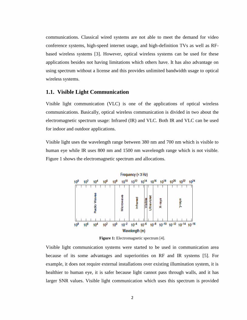
Visible light uses the wavelength range between 380 nm and 700 nm which is visible to

human eye while IR uses 800 nm and 1500 nm wavelength range which is not visible.

Figure 1 shows the electromagnetic spectrum and allocations.

Figure 1: Electromagnetic spectrum [4].

Visible light communication systems were started to be used in communication area

because of its some advantages and superiorities on RF and IR systems [5]. For

example, it does not require external installations over existing illumination system, it is

healthier to human eye, it is safer because light cannot pass through walls, and it has

larger SNR values. Visible light communication which uses this spectrum is provided

3

with white LEDs. White LEDs provide another advantage, which is double-purpose

usage, to visible light communication systems since they are also used for illumination

[6]. Studies on VLC systems have gained momentum because of all these and other

advantages of VLC. Visible light communication systems are widely used for indoor

applications and it does not give acceptable results for outdoor applications. It has not

only indoor applications such as airplane usage and video conference but also outdoor

applications such as car to car communication [7].

Visible light communication has very old history. For instance, US military used

heliograph, which can be defined as wireless solar telegraph, in 1880s. The main

principle of heliograph was based on sunlight; signals obtained with flashes of sunlight

which were reflected by a mirror. Generally Morse code was used for those signals.

After that, Alexander Graham Bell achieved transmitting speech using modulated

sunlight and this invention was called as a photophone in 1880. This was the main

corner stone for visible light communication because it was understood that visible light

can be used for data transmission after this invention. Bell obtained a patent regarding

this invention which was entitled “Apparatus for Signaling and Communicating, called

Photophone” in 1880 [8].

However, studies gained momentum in 2003 in Keio University by transmitting data

using LEDs. For this purpose Nakagawa Laboratory was established. After that,

numerous studies have performed regarding visible light communication in Nakagawa

Laboratory and all over the world. Also, Visible Light Communication Consortium was

established same year.

In 2010, 500 Mbit/s transmission was demonstrated using white LED by research group

from Siemens and Fraunhofer Institute for Telecommunications, and this transmission

was performed for 5 meters.

In 2012, VLC was standardized by conducting IEEE 802.15 which is called as IEEE

802.15.7. Its modulation schemes and dimming supports are given in the study [9].

4

In 2015, Philips and Carrefour supermarkets were collaborated to use visible light

communication for shoppers’. This is very important development for visible light

communication because it became an industrial application with this project.

In the literature, there are numerous important studies regarding visible light

communication [10-19].

1.2. Organization of Thesis

The thesis starts with Introduction and continues with five different chapters.

Chapter 2 is Optical Power Distribution that includes light sources such as light emitting

diode (LED) and laser diode. LED’s general structure and its mathematical model about

optical power are given in this chapter. Also, structure of laser diode and its transmitted

optical power calculations are mentioned. Finally, calculations regarding optical power

at the receiver part are given in this chapter.

Chapter 3 is Modulation Methods that consists of optical modulators such as electro-

optic modulators, electro-absorption modulators, and interferometric modulators which

are Mach-Zender and Fabry-Pérot. In addition to this, digital modulation techniques

such as amplitude shift keying (ASK), phase shift keying (PSK), pulse position

modulation (PPM), pulse code modulation (PCM), and quadrature amplitude modulation

(QAM).

Chapter 4 is Orthogonal Frequency Division Multiplexing (OFDM) and Orthogonal

Frequency Division Multiple Access (OFDMA). In this chapter, OFDM and OFDMA

models and regarding mathematical backgrounds are given.

Chapter 5 is Simulation Studies that includes optical power distribution, 64-QAM

OFDM system, and 64-QAM OFDMA system. Global parameters, components and their

system parameters are introduced in this chapter. Also, there is Results and Discussions

part which consists of results about the studies performed and discussions about the

results. Chapter 6 is Conclusion which has brief conclusion about studies and results.

5

CHAPTER TWO

OPTICAL POWER DISTRIBUTION

Optical power distribution is very important parameter while designing optical wireless

communication system, especially visible light communications because data

transmission is provided by light. If there is no enough optical power on the surface

where communication system is constructed, data cannot be transmitted. For example,

when a room is used to communicate using visible light, almost every point has to

achieve at least required minimum optical power so distribution of optical power plays

important role. Also, this power should be distributed uniformly to obtain better

communication system. There will be dead zones which have no required minimum

optical power and minimizing such kind of dead zones is another vital factor. To achieve

better communication systems, uniformity of optical power must be grater while amount

of dead zones must be lower.

In this chapter, properties of light will be covered firstly for background information.

Then, light sources which are LED and laser will be introduced briefly with their

properties. After defining some important laws such as Lambert’s emission law,

mathematical model for both transmitted and received optical power will be covered.

These mathematical models will be used in simulation system for optical power

distribution in the last chapter.

2.1. Light Sources

When the state of an electron is changed from higher energy level to lower energy level,

there will be excess of energy, which means that energy is generated. This excess of

energy is generally emitted in the form of light, and there are two types of light emission

which are spontaneous emission and stimulated emission [10].

6

In the spontaneous emission case, the energy level of an electron increased to the higher

energy level, then the electron spontaneously come back to the lower energy level

because lower energy levels are more stable than higher energy levels. Hence, light is

emitted spontaneously after this process. According to [10], the wavelength of this

emitted light can be known, but direction and phase cannot.

On the other hand, in the case of stimulated emission, after increasing the energy level of

the electron to the higher level, it can stay there for a while. When a photon occurs to

stimulate this electron, it emits its energy as another photon. All these processes happen

before the electron come back to more stable energy level spontaneously. In the case of

stimulated emission, the direction, phase, and wavelength of emitted photon are equal to

the stimulating photon.

There are two kinds of light sources which are light emitting diode (LED) and light

amplification by the stimulated emission of radiation (LASER). However, laser diodes

instead of laser is covered in this chapter.

1.2.1. Light-Emitting Diode (LED)

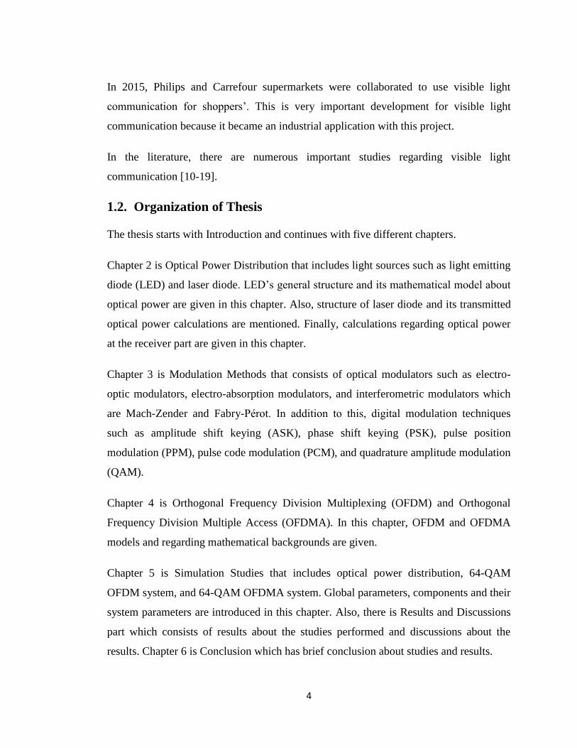
LEDs produce an output light using the principle of spontaneous emission which is

based on radiative recombination. In this process, a diode is forward biased and

electrons and holes are in the active region of the diode. Hence, LEDs generate

incoherent light and they do not have any threshold current to produce light [11]. In the

process of spontaneous emission in LED, spontaneous photon generation rate must be

equal to the spontaneous electron recombination rate because of the structure of LED

[12]. In Figure 2, general structure of an LED is shown.

Because LEDs are made from semiconductor materials which are used in all light

sources, they satisfy the properties of semiconductor diodes. The wavelength of the

output light of LED is dependent to the band-gap energy, but they have an inverse

proportionality. The equation of the wavelength of emitted light from LED is given in

[10].

7

Figure 2: Light emitting diode [11].

(2.1)

In this equation, represents the wavelength of emitted light, is Planks constant, is

speed of light, and is the photon energy. As understood from this equation,

wavelength decreases when energy increases. According to [12], when a photon is

emitted, the equation is obtained under steady-state conditions. This equation is as

follows.

(2.2)

In this equation, , , , , , , are fraction, injected current, electric charge,

volume of the active region, spontaneous recombination rate, nonradiative

recombination rate, and carrier leakage rate, respectively. As seen from this equation,

the rate of injected electrons consists of the spontaneous recombination, non-radiative

recombination, and carrier leakage. There is no parameter for stimulated recombination

8

in this equation because the working principle of an LED is directly based on a

spontaneous emission.

After defining radiative efficiency, , an optical power, , which is generated after

spontaneous emission process can be calculated as follows and all these calculations are

given in [12].

(2.3)

(2.4)

LEDs are commonly used in communication systems as well as other areas due to the

fact that it has various advantages. For instance, they are very cost effective because

LEDs are cheap components when compared to other light sources, such as laser, in

communication area.

In the perspective of characteristics of LED, it has less output power than laser.

Moreover, it produces wide spectrum because it does not produce a single wavelength. It

also produces incoherent light, hence it needs lens to focus and this brings a

disadvantage to LED. LED can be used with both analog and digital modulations, but it

cannot reach gigabit speed in digital modulation [10]. In Figure 3, commercially

available LEDs in different colors are shown.

LEDs have wide range of application area after the usage of blue color in LED. RGB

(Red Green Blue) LEDs are used commonly in illumination systems, signalization

systems, and architectures because of their life are very long. With the combination of

this RGB LEDs, every color can be produced such as white light. This is one of the most

important techniques of the production of white light.

9

Figure 3: LEDs in different colors [13].

1.2.2. Laser Diodes

Laser is the abbreviation of “light amplification by stimulated emission of radiation” and

it is developed to provide single-color coherent light. It was firstly constructed by

Theodore H. Maiman at Hughes Laboratories after the theoretical studies of Charles

Hard Townes and Arthur Leonard Schawlow. There are various laser types in the

literature such as gas laser, solid-state laser, fiber laser, photonic crystal laser,

semiconductor laser, dye laser, and doped fiber laser [14]. In this thesis, semiconductor

lasers which are also known as laser diodes are considered because their commonly

usage in the communication field.

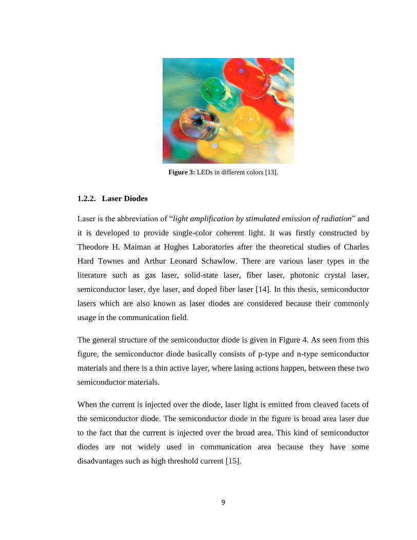
The general structure of the semiconductor diode is given in Figure 4. As seen from this

figure, the semiconductor diode basically consists of p-type and n-type semiconductor

materials and there is a thin active layer, where lasing actions happen, between these two

semiconductor materials.

When the current is injected over the diode, laser light is emitted from cleaved facets of

the semiconductor diode. The semiconductor diode in the figure is broad area laser due

to the fact that the current is injected over the broad area. This kind of semiconductor

diodes are not widely used in communication area because they have some

disadvantages such as high threshold current [15].

10

Figure 4: General structure of broad-area semiconductor laser [16].

Semiconductor lasers are also based on stimulated emission process which is valid for

other types of lasers. There are important advantages of stimulated emission as

providing high output power because of the nature of coherent light. Furthermore,

semiconductor lasers have the property of direct modulation at high frequencies such as

a few tens of GHz degrees. In addition to these advantages, they have also high coupling

efficiency due to the narrow angular spread of the output beam [15]. All these structural

properties provide extra advantages to laser when compared to LED, hence they are

widely used in communication area.

According to [15], stimulated emission occurs when a population inversion is satisfied

which is defined as having more members in the exited state than the lower state. There

are some fundamental calculations for semiconductor lasers given in [15].

The first one is the optical gain; the peak gain can be calculated as follows.

(2.5)

In this equation, represents the peak value of gain, represents the injected carrier

density, represents the differential gain, and represents the transparency value of

11

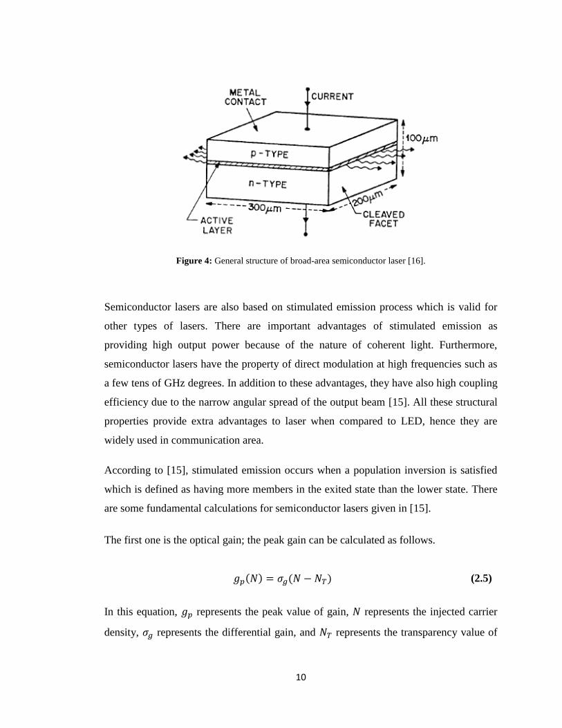
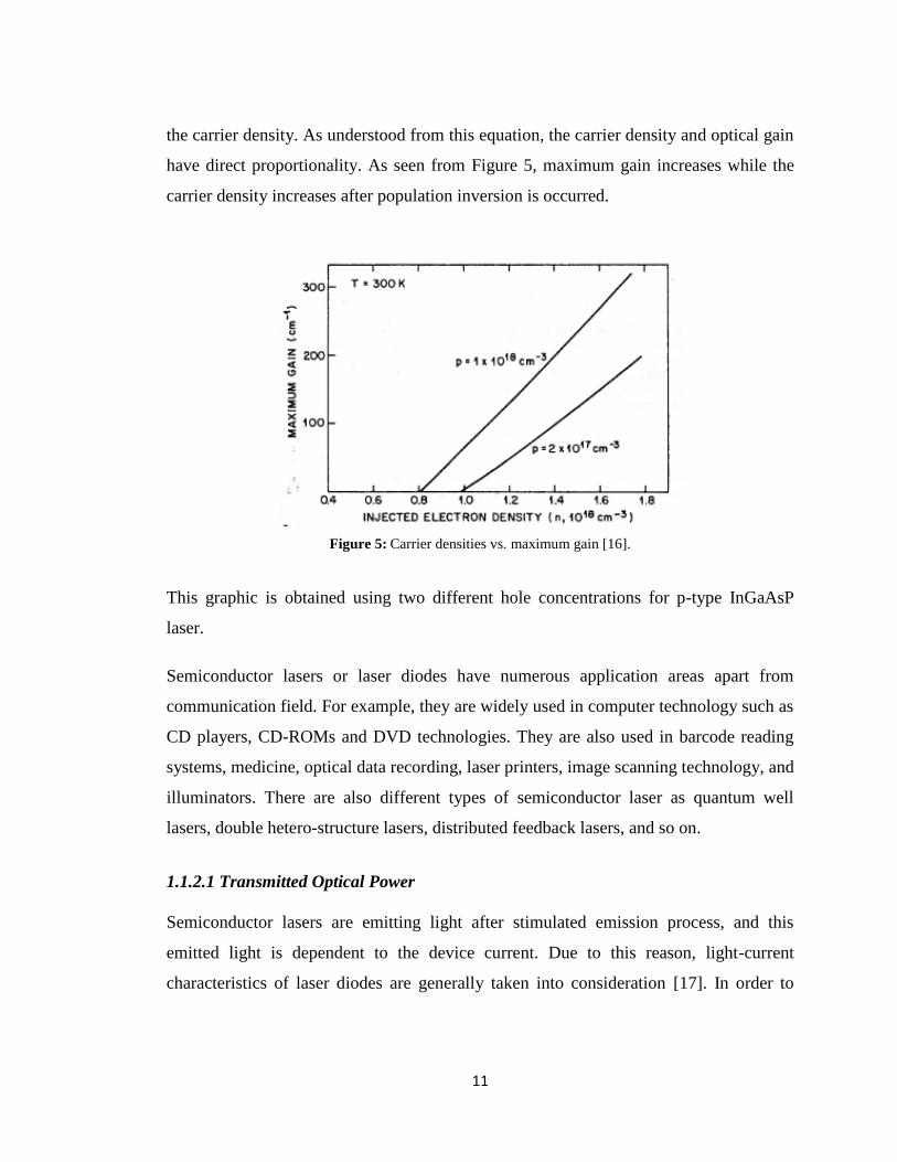
the carrier density. As understood from this equation, the carrier density and optical gain

have direct proportionality. As seen from Figure 5, maximum gain increases while the

carrier density increases after population inversion is occurred.

Figure 5: Carrier densities vs. maximum gain [16].

This graphic is obtained using two different hole concentrations for p-type InGaAsP

laser.

Semiconductor lasers or laser diodes have numerous application areas apart from

communication field. For example, they are widely used in computer technology such as

CD players, CD-ROMs and DVD technologies. They are also used in barcode reading

systems, medicine, optical data recording, laser printers, image scanning technology, and

illuminators. There are also different types of semiconductor laser as quantum well

lasers, double hetero-structure lasers, distributed feedback lasers, and so on.

1.1.2.1 Transmitted Optical Power

Semiconductor lasers are emitting light after stimulated emission process, and this

emitted light is dependent to the device current. Due to this reason, light-current

characteristics of laser diodes are generally taken into consideration [17]. In order to

12

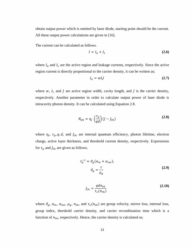
obtain output power which is emitted by laser diode, starting point should be the current.

All these output power calculations are given in [16].

The current can be calculated as follows.

(2.6)

where and are the active region and leakage currents, respectively. Since the active

region current is directly proportional to the carrier density, it can be written as;

(2.7)

where , , and are active region width, cavity length, and is the carrier density,

respectively. Another parameter in order to calculate output power of laser diode is

intracavity photon density. It can be calculated using Equation 2.8.

(2.8)

where , , and are internal quantum efficiency, photon lifetime, electron

charge, active layer thickness, and threshold current density, respectively. Expressions

for and are given as follows.

(2.9)

(2.10)

where , , , , , and are group velocity, mirror loss, internal loss,

group index, threshold carrier density, and carrier recombination time which is a

function of , respectively. Hence, the carrier density is calculated as;

13

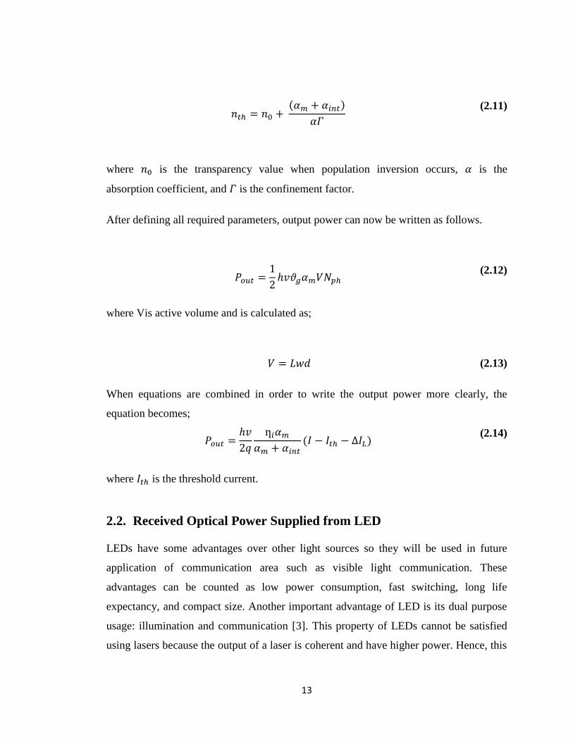
(2.11)

where is the transparency value when population inversion occurs, is the

absorption coefficient, and is the confinement factor.

After defining all required parameters, output power can now be written as follows.

(2.12)

where Vis active volume and is calculated as;

(2.13)

When equations are combined in order to write the output power more clearly, the

equation becomes;

(2.14)

where is the threshold current.

2.2. Received Optical Power Supplied from LED

LEDs have some advantages over other light sources so they will be used in future

application of communication area such as visible light communication. These

advantages can be counted as low power consumption, fast switching, long life

expectancy, and compact size. Another important advantage of LED is its dual purpose

usage: illumination and communication [3]. This property of LEDs cannot be satisfied

using lasers because the output of a laser is coherent and have higher power. Hence, this

14

can be dangerous to human health. LEDs are the main candidate of visible light

communication systems due to their dual purpose usage property as well as fast

switching property. Fast switching is one of the most important features of light sources

because data is obtaining by switching the light source. For example, data is 0 digitally

when the light source is closed and data is 1 digitally when the light source is opened.

By performing such kind of switching, overall digital information is obtained.

Output power of an LED is very important factor while designing the visible light

communication system since data transferred through light. There must be enough

optical power at the receiver side to obtain the transmitted information. If there is no

enough received optical power on any area, this kind of areas are called as dead zones.

In ideal visible light communication system inside a room, there must be no dead zones.

However, dead zones are occurred in real systems and they must be minimized in term

of their amount. Hence, the mathematical models are needed for both transmitted and

received optical powers to minimize the dead zones by performing some simulations.

In these mathematical models, there are some parameters regarding LEDs properties

such as half-angle illuminance. These parameters can be known using data sheets of

LEDS which have all the features of any special LED. After deciding the LED type

which will be used in communication system as a light source, its special features is

used to simulate the overall system to see how the optical power is distributed on the

receiver plane.

In [3], mathematical models for visible light communication are given. One of these

models is the received optical power.

The luminous intensity which expresses the brightness of LED is as follows.

(2.15)

15

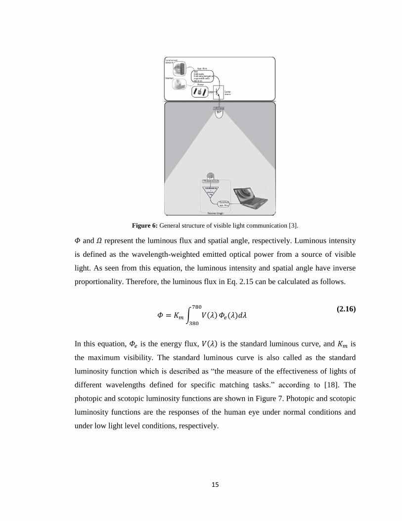
Figure 6: General structure of visible light communication [3].

and represent the luminous flux and spatial angle, respectively. Luminous intensity

is defined as the wavelength-weighted emitted optical power from a source of visible

light. As seen from this equation, the luminous intensity and spatial angle have inverse

proportionality. Therefore, the luminous flux in Eq. 2.15 can be calculated as follows.

(2.16)

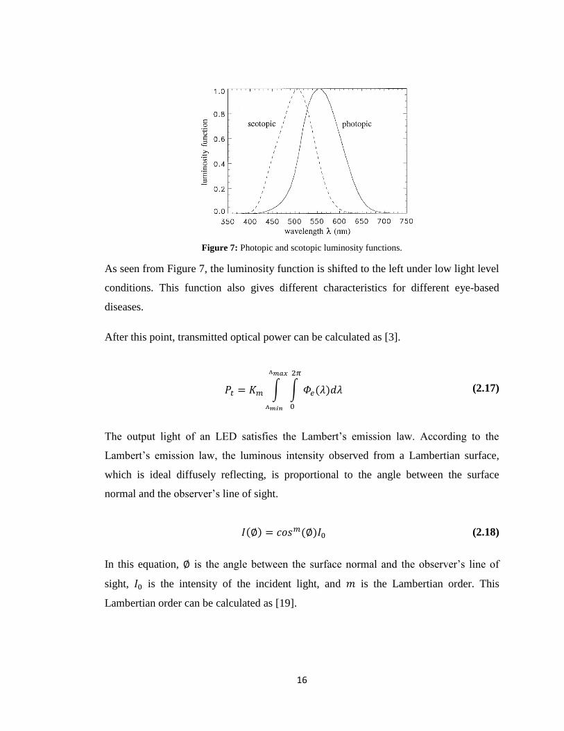
In this equation, is the energy flux, is the standard luminous curve, and is

the maximum visibility. The standard luminous curve is also called as the standard

luminosity function which is described as “the measure of the effectiveness of lights of

different wavelengths defined for specific matching tasks.” according to [18]. The

photopic and scotopic luminosity functions are shown in Figure 7. Photopic and scotopic

luminosity functions are the responses of the human eye under normal conditions and

under low light level conditions, respectively.

16

Figure 7: Photopic and scotopic luminosity functions.

As seen from Figure 7, the luminosity function is shifted to the left under low light level

conditions. This function also gives different characteristics for different eye-based

diseases.

After this point, transmitted optical power can be calculated as [3].

(2.17)

The output light of an LED satisfies the Lambert’s emission law. According to the

Lambert’s emission law, the luminous intensity observed from a Lambertian surface,

which is ideal diffusely reflecting, is proportional to the angle between the surface

normal and the observer’s line of sight.

(2.18)

In this equation, is the angle between the surface normal and the observer’s line of

sight, is the intensity of the incident light, and is the Lambertian order. This

Lambertian order can be calculated as [19].

17

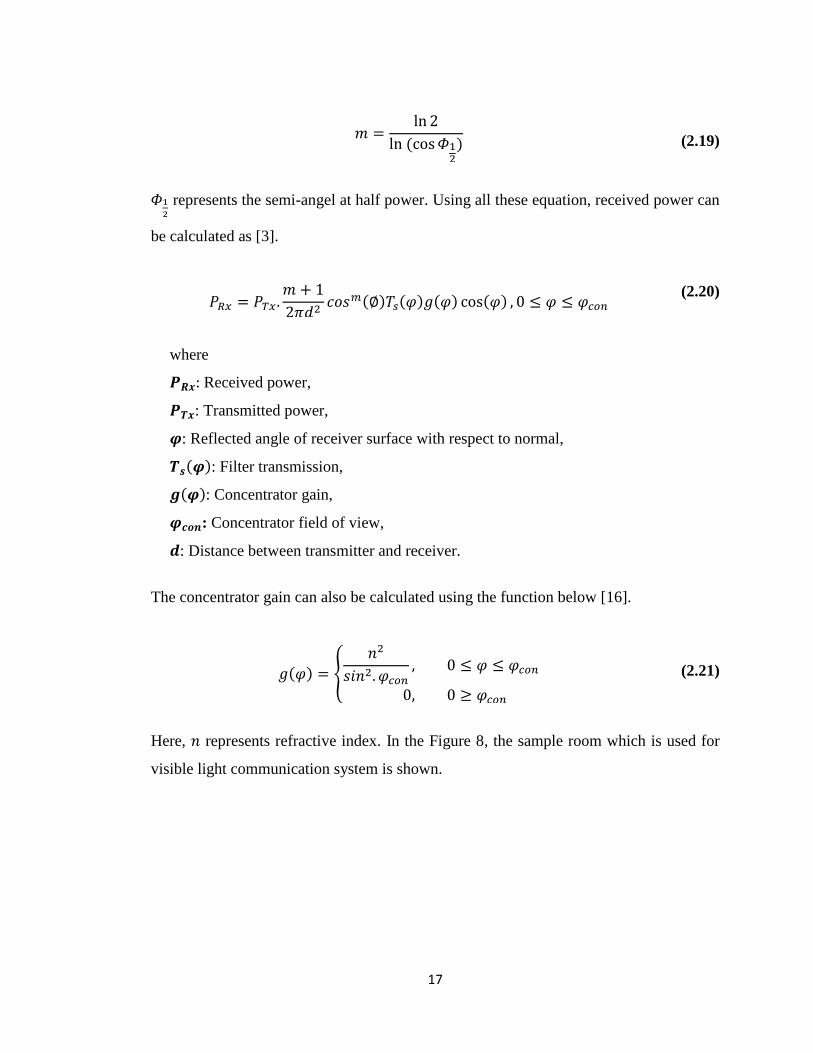
(2.19)

represents the semi-angel at half power. Using all these equation, received power can

be calculated as [3].

(2.20)

where

Received power,

: Transmitted power,

: Reflected angle of receiver surface with respect to normal,

: Filter transmission,

: Concentrator gain,

: Concentrator field of view,

: Distance between transmitter and receiver.

The concentrator gain can also be calculated using the function below [16].

(2.21)

Here, represents refractive index. In the Figure 8, the sample room which is used for

visible light communication system is shown.

18

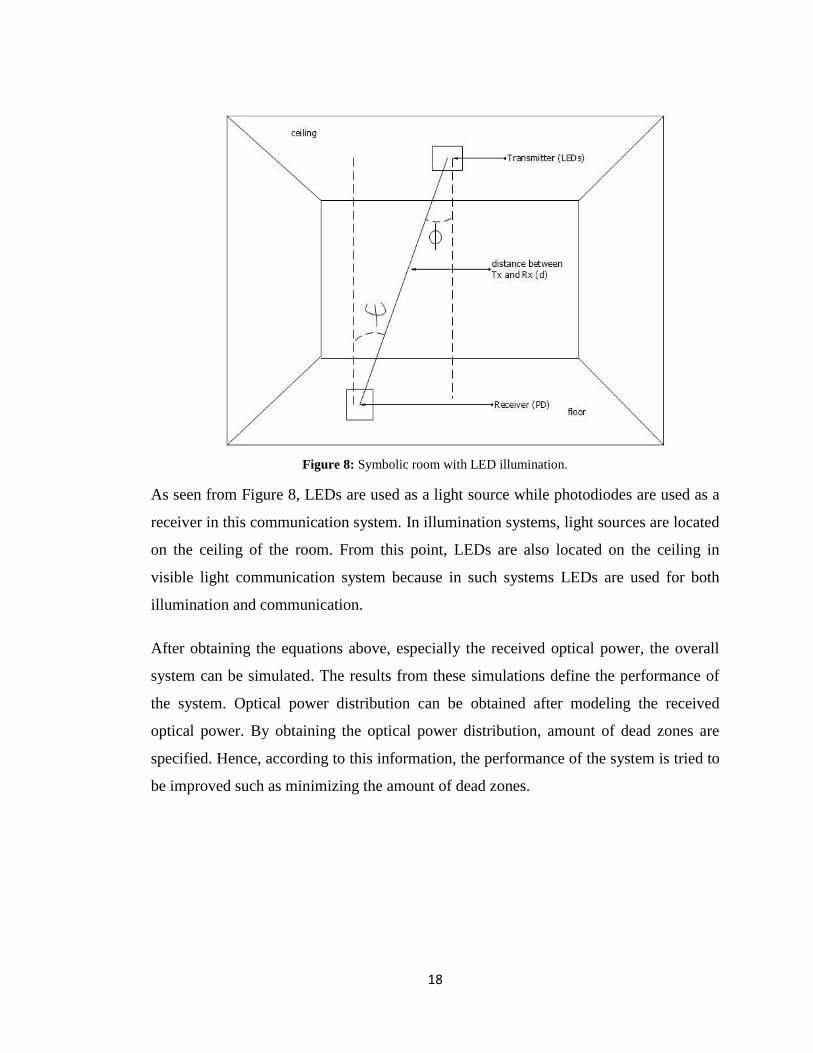
Figure 8: Symbolic room with LED illumination.

As seen from Figure 8, LEDs are used as a light source while photodiodes are used as a

receiver in this communication system. In illumination systems, light sources are located

on the ceiling of the room. From this point, LEDs are also located on the ceiling in

visible light communication system because in such systems LEDs are used for both

illumination and communication.

After obtaining the equations above, especially the received optical power, the overall

system can be simulated. The results from these simulations define the performance of

the system. Optical power distribution can be obtained after modeling the received

optical power. By obtaining the optical power distribution, amount of dead zones are

specified. Hence, according to this information, the performance of the system is tried to

be improved such as minimizing the amount of dead zones.

19

CHAPTER THREE

MODULATION AND ACCESS METHODS

Communication between people almost involves whole daily life because people contact

each other using communication technologies. The main objective of the communication

systems is transmitting data from transmitter to receiver. Although data to be transmitted

is mostly the baseband signal which has low frequencies, the channel that is used as a

medium for transmission is needed high frequencies which are pass-band frequencies.

Because of this reason, signal must be made suitable to the channel in order to perform

the transmission between transmitter and receiver.

Modulation is used for this purpose which is making the data suitable to the transmission

channel by shifting the frequency of the signal from baseband to pass-band frequencies.

After this modulation process, data can be transmitted easily. To perform this frequency

shift, high frequency carrier signals are used.

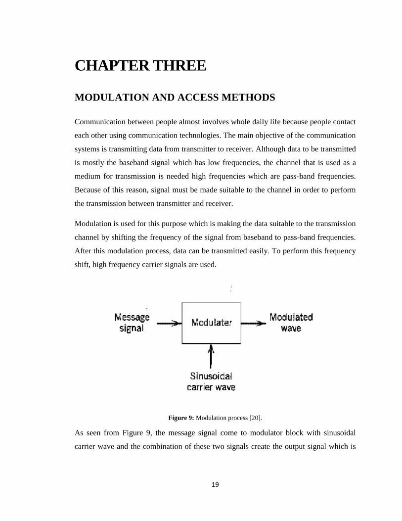
Figure 9: Modulation process [20].

As seen from Figure 9, the message signal come to modulator block with sinusoidal

carrier wave and the combination of these two signals create the output signal which is

20

modulated wave. The modulation process seen on the figure is the continuous wave

modulation technique which uses continuous waves such as sinusoidal wave as a carrier.

Modulation can be classified into numerous subsets such as analog modulation, digital

modulation, optical modulation, and multi-carrier modulation. All these modulation

techniques have some advantages/disadvantages and properties in terms of their system

performances. Each of these modulation techniques can be used according to certain

application. For example, multi-carrier modulation techniques should be used if the

channel efficiency is needed in the proposed system.

In this chapter, the classification of modulation techniques will be as follows: Optical

modulation and digital modulation. After introducing all these techniques, multi-carrier

access methods such as time division multiple access (TDMA) and frequency division

multiple access (FDMA) will be introduced.

3.1. Optical Modulators

Optical modulators are devices to modulate light by controlling its properties such as

intensity, polarization, and phase. For wired communication systems, the electrical

signal is used to transmit the data from transmitter to receiver. The main conveying thing

is electrical signal, and this electrical signal is passing through a transmission medium

such as copper to accomplish the data transmission. Before transmission happens, the

electrical signal is modulated in order to make it suitable for the channel. There are

various modulation techniques regarding such kind of communication system such as

amplitude modulation, phase modulation, frequency modulation, and so on.

For the optical communication systems, the transmission medium may be fiber for wired

communication, and it may be air for wireless communication. Moreover, the data to be

transmitted is conveyed by light for optical communication systems. There is also

modulation process for optical communication systems as in the wired communications.

21

There are two main class for optical modulators; direct modulation and external

modulation. However, direct modulation cannot meet the increasing speed requirements

for some applications. Because of this reason, only external optical modulators will be

introduced in this part.

Electro-optic modulators, electro-absorption modulators, acousto-optic modulators, and

interferometric modulators are main modulator types for light-base communication

systems.

3.1.1. Electro-Optic Modulators

Electro-optic modulators are devices that are working with the principle of electro-optic

effect. There are some unique materials which are changing their optical properties when

electric field is applied. When low frequency or dc electric field is applied to such kind

of certain materials, their refractive indices are changed, and this change originates the

fundamentals of electro-optic effect. Although the change on refractive index of the

material is not large, there is an important effect on light which is travelling through the

medium [21].

If electric field is applied to the electro-optic material while light is passing through it,

there will be a change on effect of the material on light. This happens because the optical

properties of the material are changed. If its properties change, its effects on light also

change.

There are two main effect of the electric field application to the electro-optic material.

One of them is known as a Pockels effect which is defined as a linear effect on refractive

index of the material with respect to electric field. In other words, there is a direct

proportionality between electric field and refractive index.

The second effect is known as a Kerr effect which defines the quadratic relationship

between electric field and refractive index. In other words, refractive index is

proportional to the square of the applied electric field [21].

22

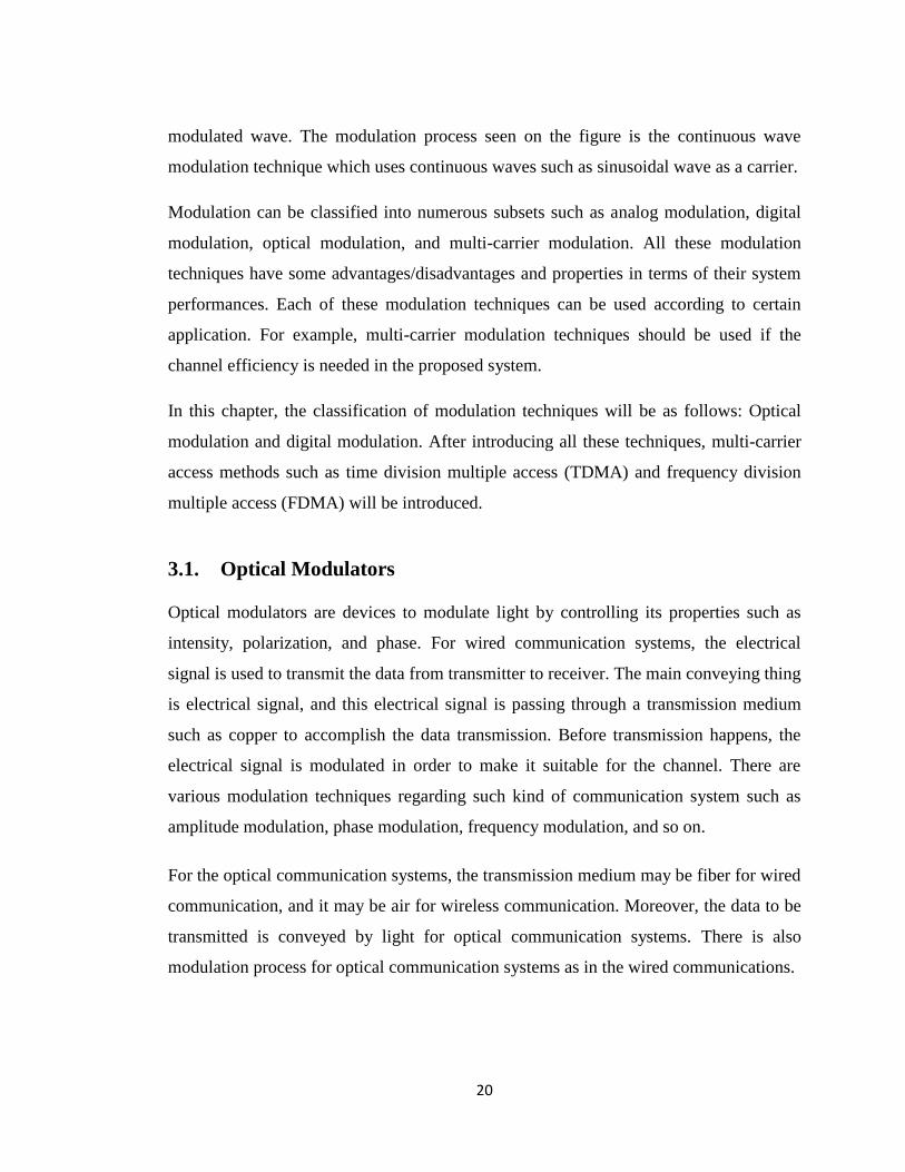
Pockels cells are developed to be used in communication systems, and they work using

Pockels effect. They are basically electro-optic crystals and light can easily travel

through them. Their control can be provided with electric voltage; when electric voltage

is applied on them, the electric field occurs. By this way, the modulation process can be

performed. In Figure 10, IRX series CdTe Pockels cells belonging to Gooch&Housego

Company is shown.

Figure 10: IRX series CdTe Pockels cells [22].

After constructing the background information about electro-optic effect and Pockels

cells, electro-optic modulators that are used in communication systems can be

introduced.

Electro-optic modulators are devices that are developed to modulate light by changing

its some main properties such as phase, power, and polarization. To perform the

modulation process, it needs some electrical signals such as electric voltage to generate

the electric field. Because of this, these modulators are also called as signal-controlled

modulators.

In order to perform phase modulation using electro-optic effect, phase of the light which

enters to the material must be changed. Assume a laser beam, which has an amplitude of

and frequency of , propagating through the material. After a sinusoidal voltage,

which has another frequency level of , is applied to the material. After combining these

two, there will be one original signal and two different sidebands which are

23

and . Then, the phase delay occurs after application of electric field using electric

voltage.

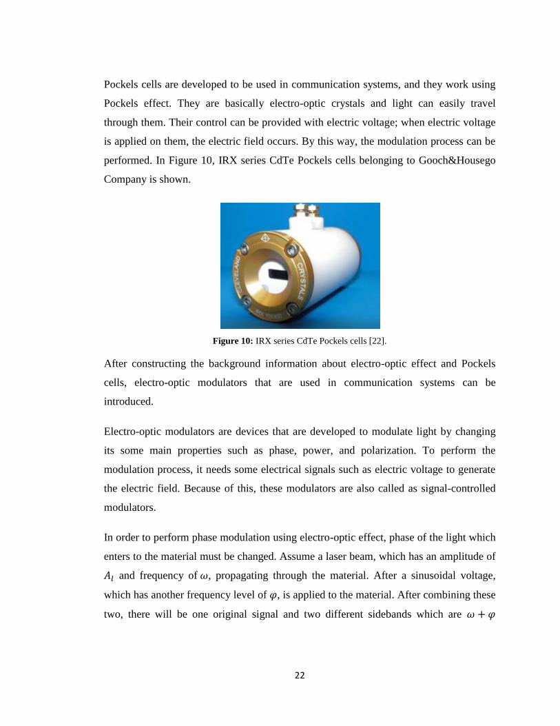
The typical phase modulators with the help of electro-optic effect are shown in Figure

11. In this figure, electro-optic material, electrodes, incident light, and modulated light

are shown clearly.

Figure 11: Phase modulator [21].

Polarization and amplitude of the incident light such as laser beam can also be

modulated using electro-optic modulators; for example, polarization of the incident light

can affect the phase delay which occurs after application of electric field.

3.1.2. Electro-Absorption Modulators

Electro-absorption modulators are devices which are using the Franz-Keldysh effect.

Franz-Keldysh theory states that optical absorption of a semiconductor material can

change when electric field is applied on it. This electric field is generated with the

application of electric voltage. Moreover, the electric field application also changes the

effective bandgap of a semiconductor material. When electric field applied to the

material, effective bandgap gets smaller. There is an important concept that is behind the

working principle of electro-absorption modulators; if the energy of the bandgap is

greater than the energy of the incident light which is entering the semiconductor

material, , the material becomes transparent. Hence, the incident light can easily

24

pass through the material. However, when electric field is applied to the material, the

material starts to absorb the incident light due to the fact that the bandgap energy gets

smaller [23].

By using the Franz-Keldysh effect, semiconductor materials can be used as modulators

for light-wave. For instance, they can modulate the intensity of the laser beam by

applying the electric field. This kind of modulators are called as electro-absorption

modulators because they use the electric field to control the intensity of the laser beam

using electric, and this process is based on absorption change in semiconductor material.

There are various advantages belonging to electro-absorption modulators. For example,

they need lower drive voltage, they can be used in applications that require high speed

modulation, and they have also integrability property [24].

3.1.3. Interferometric Modulators

Interferometers are devices that are used in optical systems commonly. They are mostly

used in optical measurements systems; in other words, they are used as optical sensors.

Normally, the interference is unwanted situation that occurs in optical systems. It affects

the system performance in a negative way. For example, it is a problem in

communication systems because of its negative effects on data transmission.

However, the interference property can be also used in a positive way. Interferometers

use the property of interference to modulate the light in order to measure some

parameters. Assume there is an incident light, and it meets with beam splitter which is

used for splitting light waves into more than one beams. After two separate light beams

occur, they travel and recombine as a property of superposition, and the phase difference

occurs. This recombination gives some information about external conditions.

There are some commonly known interferometric modulators such as Mach-Zender

modulator, Fabry-Pérot modulator, and Michelson modulator. In the remaining part of

this section, some of these modulators will be introduced.

25

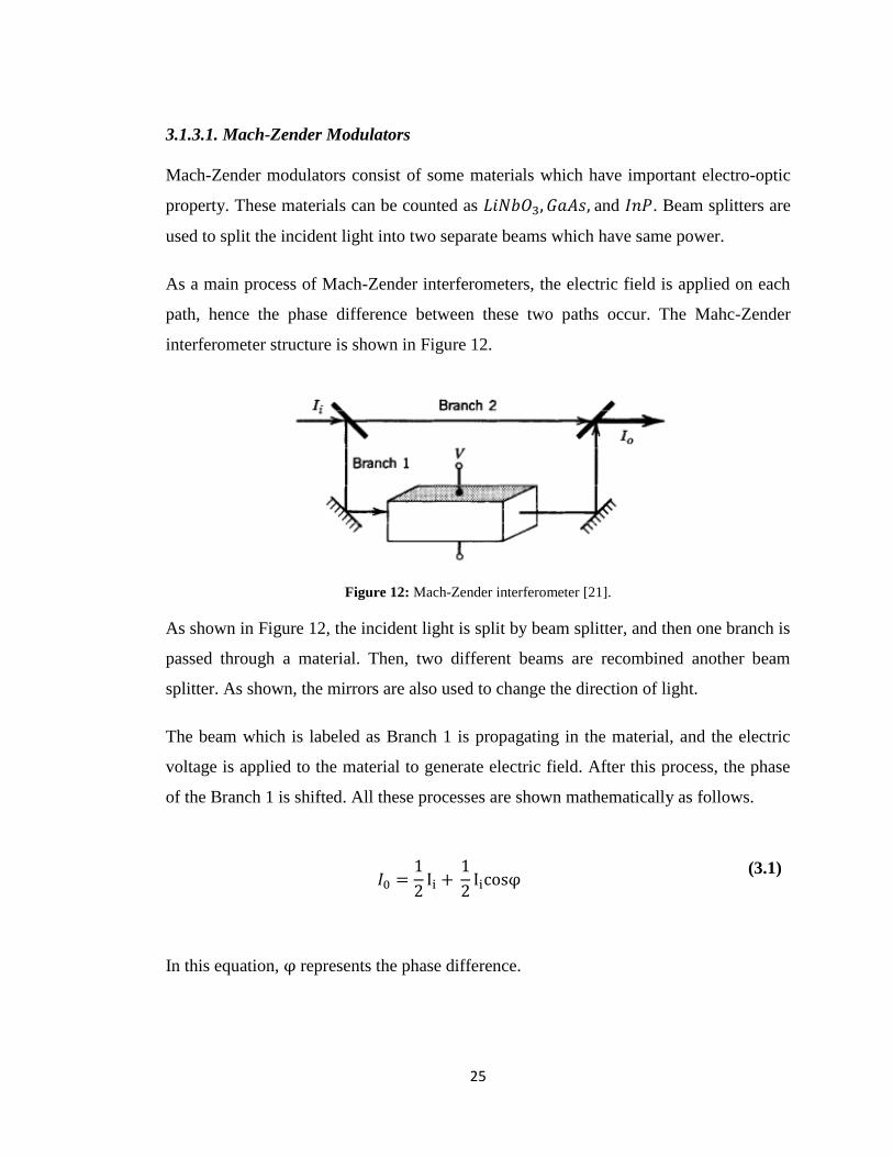
3.1.3.1. Mach-Zender Modulators

Mach-Zender modulators consist of some materials which have important electro-optic

property. These materials can be counted as and . Beam splitters are

used to split the incident light into two separate beams which have same power.

As a main process of Mach-Zender interferometers, the electric field is applied on each

path, hence the phase difference between these two paths occur. The Mahc-Zender

interferometer structure is shown in Figure 12.

Figure 12: Mach-Zender interferometer [21].

As shown in Figure 12, the incident light is split by beam splitter, and then one branch is

passed through a material. Then, two different beams are recombined another beam

splitter. As shown, the mirrors are also used to change the direction of light.

The beam which is labeled as Branch 1 is propagating in the material, and the electric

voltage is applied to the material to generate electric field. After this process, the phase

of the Branch 1 is shifted. All these processes are shown mathematically as follows.

(3.1)

In this equation, represents the phase difference.

26

(3.2)

As understood from all these processes, the Mach-Zender performs a phase modulation.

However, this phase modulation can be turned out to be an intensity modulation by

adjusting the optical path difference [21].

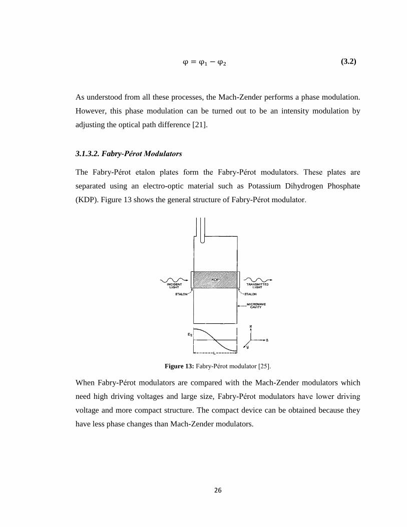
3.1.3.2. Fabry-Pérot Modulators

The Fabry-Pérot etalon plates form the Fabry-Pérot modulators. These plates are

separated using an electro-optic material such as Potassium Dihydrogen Phosphate

(KDP). Figure 13 shows the general structure of Fabry-Pérot modulator.

Figure 13: Fabry-Pérot modulator [25].

When Fabry-Pérot modulators are compared with the Mach-Zender modulators which

need high driving voltages and large size, Fabry-Pérot modulators have lower driving

voltage and more compact structure. The compact device can be obtained because they

have less phase changes than Mach-Zender modulators.

27

3.2. Digital Modulation

Analog modulation techniques are old fashioned modulation techniques because they

have some problems such as bandwidth information capacity and security. Digital

modulation techniques can solve some of the problems that analog modulation has. For

instance, there is more information capacity in the digital communication if it is

compared with the analog communication. Furthermore, quality of the overall

communication system can be improved while providing higher data security using

digital modulations [26]. As mentioned earlier, the main discussion topics in

communication technologies are bandwidth efficiency and power considerations. Digital

modulation techniques are more suitable to overcome these problems than analog

modulation techniques.

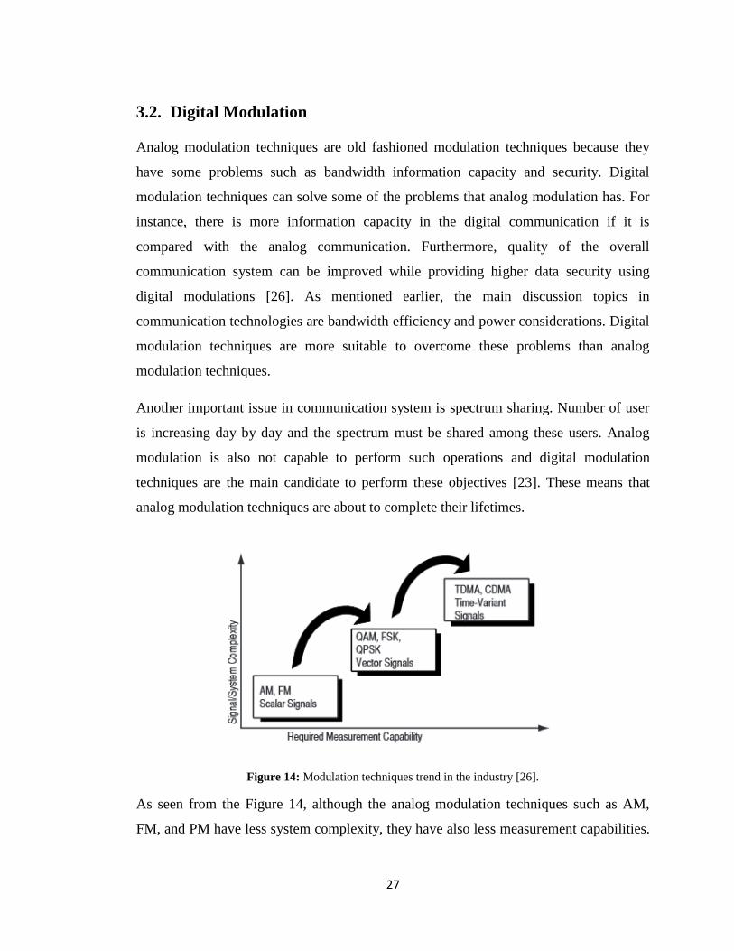
Another important issue in communication system is spectrum sharing. Number of user

is increasing day by day and the spectrum must be shared among these users. Analog

modulation is also not capable to perform such operations and digital modulation

techniques are the main candidate to perform these objectives [23]. These means that

analog modulation techniques are about to complete their lifetimes.

Figure 14: Modulation techniques trend in the industry [26].

As seen from the Figure 14, although the analog modulation techniques such as AM,

FM, and PM have less system complexity, they have also less measurement capabilities.

28

Because of this kind of reasons, trend in the industry is going from analog modulation to

digital modulation methods [26].

In this part of the chapter, commonly used digital communication techniques will be

introduced with some mathematical backgrounds.

3.2.1. Amplitude-Shift Keying (ASK)

Amplitude shift keying is one of the most commonly used digital modulation techniques.

In this modulation technique, there are two or more discrete amplitude levels to combine

carrier signal which is generally sinusoids [27]. There are basically two types of

amplitude shift keying modulation methods which are binary-ASK (BASK) and M-Ary

ASK (M-ASK).

In the BASK, there are two levels which are 1 and 0. The BASK signal is represented as

follows.

(3.3)

In this equation, is the amplitude which is constant, is the message signal which

has values of 1 and 0 only, is the frequency of the carrier signal. Also, can be

defined as time duration. The power becomes:

(3.4)

then

(3.5)

While the energy can be calculated as

(3.6)

29

which is the multiplication of the time and power, BASK signal can be written as

follows.

(3.7)

Moreover, the Fourier transform of this BASK signal is as follows.

(3.8)

Since BASK is the switching the amplitude of the carrier signal between on and off

states, it is also called as on-off keying (OOK). As seen from Eq. 3.8, the frequency of

the message signal is shifted on the spectrum to by multiplying the carrier signal [28].

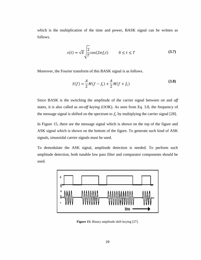
In Figure 15, there are the message signal which is shown on the top of the figure and

ASK signal which is shown on the bottom of the figure. To generate such kind of ASK

signals, sinusoidal carrier signals must be used.

To demodulate the ASK signal, amplitude detection is needed. To perform such

amplitude detection, both tunable low pass filter and comparator components should be

used.

Figure 15: Binary amplitude shift keying [27].

30

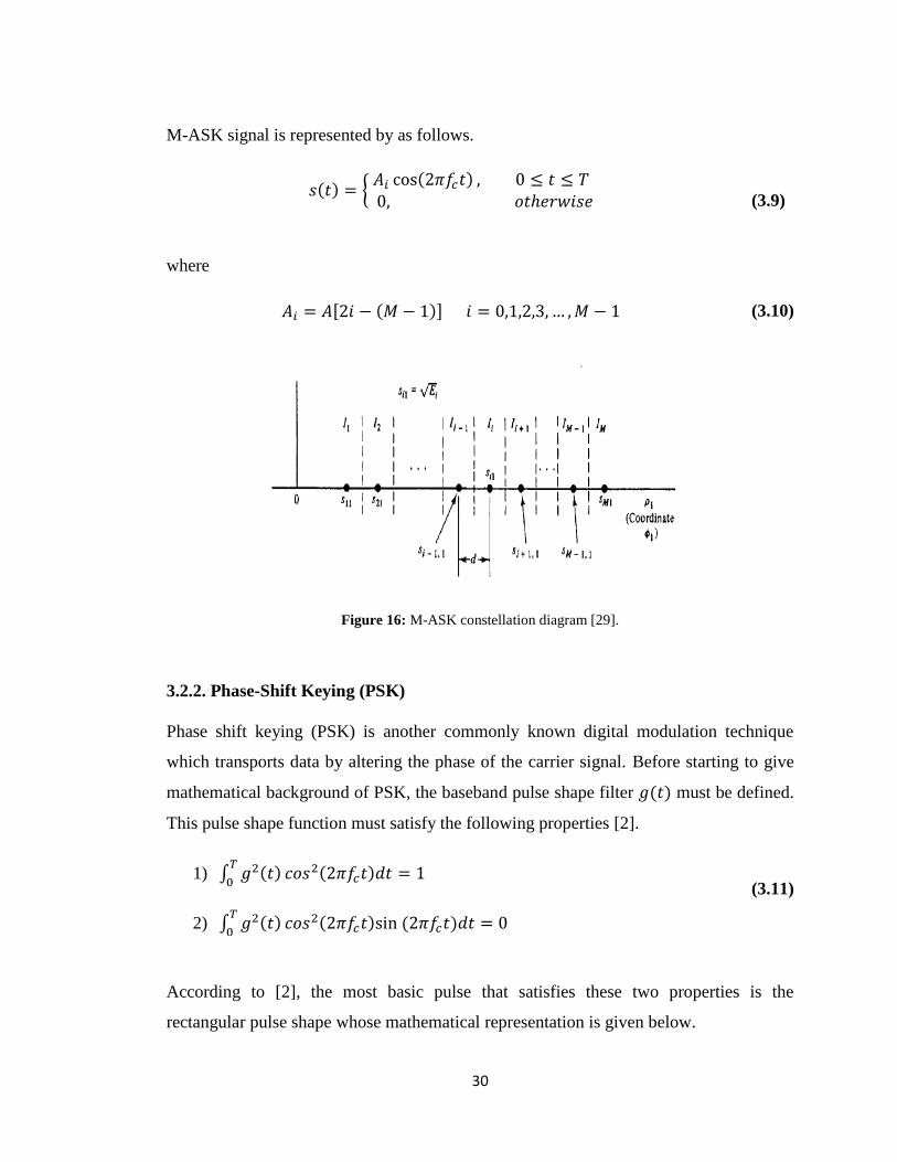
M-ASK signal is represented by as follows.

(3.9)

where

(3.10)

Figure 16: M-ASK constellation diagram [29].

3.2.2. Phase-Shift Keying (PSK)

Phase shift keying (PSK) is another commonly known digital modulation technique

which transports data by altering the phase of the carrier signal. Before starting to give

mathematical background of PSK, the baseband pulse shape filter must be defined.

This pulse shape function must satisfy the following properties [2].

1)

2)

(3.11)

According to [2], the most basic pulse that satisfies these two properties is the

rectangular pulse shape whose mathematical representation is given below.

31

where

(3.12)

After defining the pulse shaper, the mathematical background of PSK can be given. The

transmitted signal can be calculated as

(3.13)

Modulation type of PSK is changing regarding M value which is calculated as

where

(3.14)

value in the Eq. 3.14 represents the number of bits to be transmitted. According to this

and values, MPSK is determined. For example, MPSK becomes 2PSK which is

also called as Binary PSK (BPSK) when and . Analogically, MPSK

become 4PSK when and this modulation type is also known as quadrature phase

shift keying (QPSK) [2].

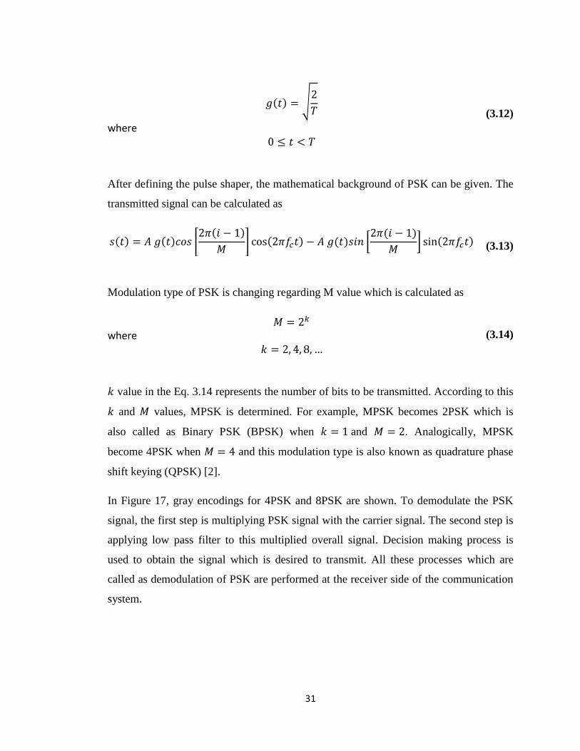
In Figure 17, gray encodings for 4PSK and 8PSK are shown. To demodulate the PSK

signal, the first step is multiplying PSK signal with the carrier signal. The second step is

applying low pass filter to this multiplied overall signal. Decision making process is

used to obtain the signal which is desired to transmit. All these processes which are

called as demodulation of PSK are performed at the receiver side of the communication

system.

32

Figure 17: 4PSK (QPSK) and 8PSK constellation diagrams [2].

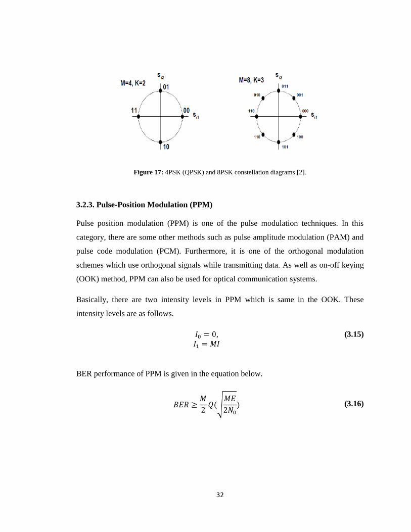
3.2.3. Pulse-Position Modulation (PPM)

Pulse position modulation (PPM) is one of the pulse modulation techniques. In this

category, there are some other methods such as pulse amplitude modulation (PAM) and

pulse code modulation (PCM). Furthermore, it is one of the orthogonal modulation

schemes which use orthogonal signals while transmitting data. As well as on-off keying

(OOK) method, PPM can also be used for optical communication systems.

Basically, there are two intensity levels in PPM which is same in the OOK. These

intensity levels are as follows.

,

(3.15)

BER performance of PPM is given in the equation below.

(3.16)

33

where and are received electrical energy and the noise power spectral density,

respectively. Also, represents the Q-function which is defined as the tail probability of

the standard normal distribution and is calculated by [30].

(3.17)

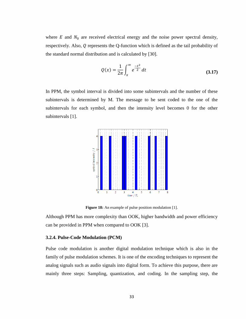
In PPM, the symbol interval is divided into some subintervals and the number of these

subintervals is determined by M. The message to be sent coded to the one of the

subintervals for each symbol, and then the intensity level becomes 0 for the other

subintervals [1].

Figure 18: An example of pulse position modulation [1].

Although PPM has more complexity than OOK, higher bandwidth and power efficiency

can be provided in PPM when compared to OOK [3].

3.2.4. Pulse-Code Modulation (PCM)

Pulse code modulation is another digital modulation technique which is also in the

family of pulse modulation schemes. It is one of the encoding techniques to represent the

analog signals such as audio signals into digital form. To achieve this purpose, there are

mainly three steps: Sampling, quantization, and coding. In the sampling step, the

34

samples of the amplitude of the analog signal are taken with some time interval. As a

second step, every sample must be quantized.

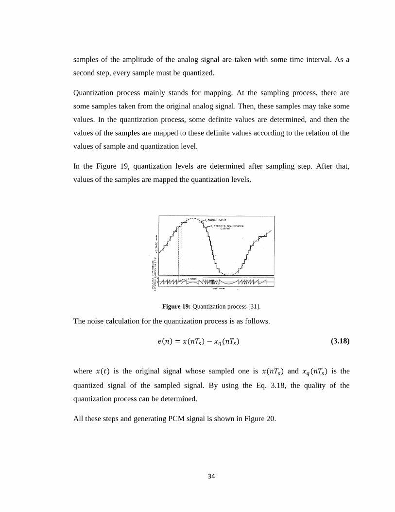
Quantization process mainly stands for mapping. At the sampling process, there are

some samples taken from the original analog signal. Then, these samples may take some

values. In the quantization process, some definite values are determined, and then the

values of the samples are mapped to these definite values according to the relation of the

values of sample and quantization level.

In the Figure 19, quantization levels are determined after sampling step. After that,

values of the samples are mapped the quantization levels.

Figure 19: Quantization process [31].

The noise calculation for the quantization process is as follows.

(3.18)

where is the original signal whose sampled one is and is the

quantized signal of the sampled signal. By using the Eq. 3.18, the quality of the

quantization process can be determined.

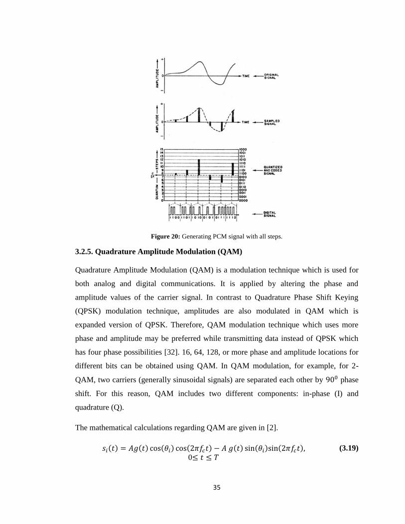
All these steps and generating PCM signal is shown in Figure 20.

35

Figure 20: Generating PCM signal with all steps.

3.2.5. Quadrature Amplitude Modulation (QAM)

Quadrature Amplitude Modulation (QAM) is a modulation technique which is used for

both analog and digital communications. It is applied by altering the phase and

amplitude values of the carrier signal. In contrast to Quadrature Phase Shift Keying

(QPSK) modulation technique, amplitudes are also modulated in QAM which is

expanded version of QPSK. Therefore, QAM modulation technique which uses more

phase and amplitude may be preferred while transmitting data instead of QPSK which

has four phase possibilities [32]. 16, 64, 128, or more phase and amplitude locations for

different bits can be obtained using QAM. In QAM modulation, for example, for 2-

QAM, two carriers (generally sinusoidal signals) are separated each other by phase

shift. For this reason, QAM includes two different components: in-phase (I) and

quadrature (Q).

The mathematical calculations regarding QAM are given in [2].

0

(3.19)

36

is the transmitted signal and is the pulse shaper. The energy is regarding the

transmitted signal is as follows.

(3.20)

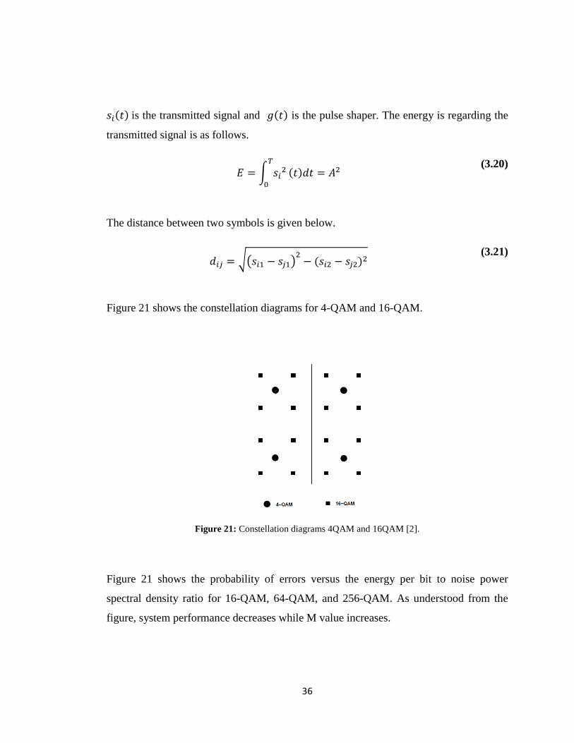
The distance between two symbols is given below.

(3.21)

Figure 21 shows the constellation diagrams for 4-QAM and 16-QAM.

Figure 21: Constellation diagrams 4QAM and 16QAM [2].

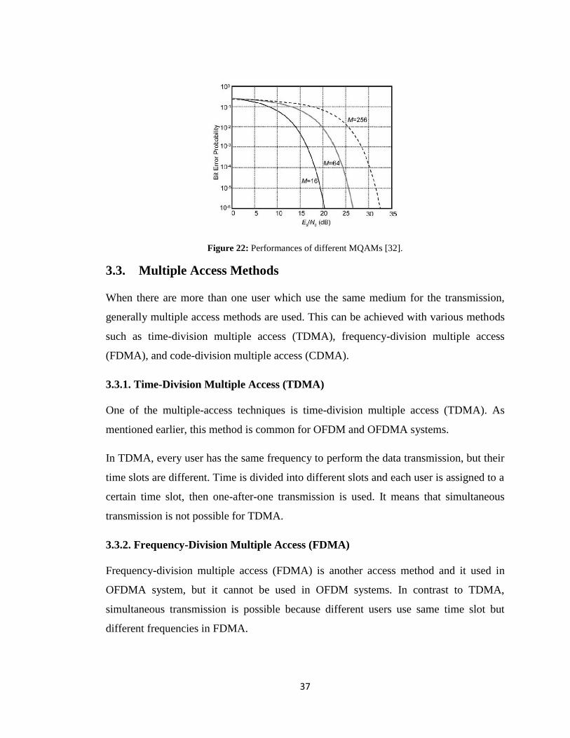
Figure 21 shows the probability of errors versus the energy per bit to noise power

spectral density ratio for 16-QAM, 64-QAM, and 256-QAM. As understood from the

figure, system performance decreases while M value increases.

37

Figure 22: Performances of different MQAMs [32].

3.3. Multiple Access Methods

When there are more than one user which use the same medium for the transmission,

generally multiple access methods are used. This can be achieved with various methods

such as time-division multiple access (TDMA), frequency-division multiple access

(FDMA), and code-division multiple access (CDMA).

3.3.1. Time-Division Multiple Access (TDMA)

One of the multiple-access techniques is time-division multiple access (TDMA). As

mentioned earlier, this method is common for OFDM and OFDMA systems.

In TDMA, every user has the same frequency to perform the data transmission, but their

time slots are different. Time is divided into different slots and each user is assigned to a

certain time slot, then one-after-one transmission is used. It means that simultaneous

transmission is not possible for TDMA.

3.3.2. Frequency-Division Multiple Access (FDMA)

Frequency-division multiple access (FDMA) is another access method and it used in

OFDMA system, but it cannot be used in OFDM systems. In contrast to TDMA,

simultaneous transmission is possible because different users use same time slot but

different frequencies in FDMA.

38

In other words, different users can share the medium for transmission at the same time,

and this is achieved by frequency division. Because OFDMA is based on both TDMA

and FDMA while OFMD is based on only TDMA, the main difference between these

techniques is simultaneous transmission.

3.3.3. Code-Division Multiple Access (CDMA)

Code-division multiple access method is can be classified as a spread spectrum method.

Similarly, more than one user can use the spectrum simultaneously, but there is a distinct

signature sequence for all users in CDMA. Pseudo-random code is used in order to

spread the bandwidth of the data, and each transmission is coded with their own pseudo-

random codes. Furthermore, receiver can distinguish the individual user from these

special codes. In CDMA, different users overlap both frequency and time domains [33].

39

CHAPTER FOUR

OFDM and OFDMA

4.1. Orthogonal Frequency Division Multiplexing (OFDM)

Orthogonal Frequency Division Multiplexing (OFDM) transmission system which is one

of the multi-channel systems provides transmission using multi-carriers. In contrast to

classical frequency division systems, sub-carriers are overlapped on the spectrum to

provide efficiency from bandwidth [34], [35].

4.1.1. Orthogonality

Orthogonality gains much importance in OFDM systems. Due to this reason,

orthogonality of signals must be investigated mathematically and systems should be

performed using such mathematical model. The starting point of these mathematical

modeling is how two signal becomes orthogonal. These calculations are given below.

Inner product of two signals must be zero to become orthogonal. For instance, assume

there are two exponential and functions which are defined between and , and

their inner product can be represent with the expression above [36].

(4.1)

If there are time-limited complex exponential signals;

(4.2)

Then, the frequencies belonging to different sub-carries are as follows.

40

,

0

(4.3)

The orthogonality;

(4.4)

Orthogonality function could be represented by Equation 4.4. After orthogonality is

guaranteed, bandwidth efficiency is ensured by overlapping the sub-carriers with each

other.

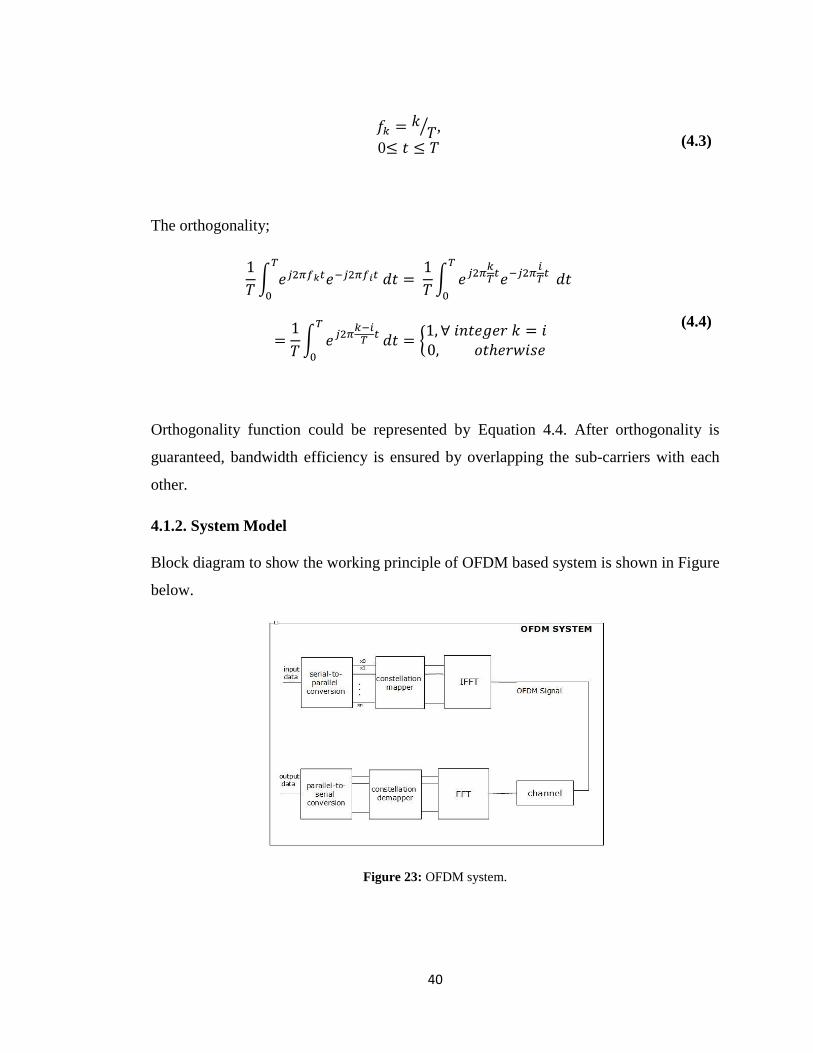
4.1.2. System Model

Block diagram to show the working principle of OFDM based system is shown in Figure

below.

Figure 23: OFDM system.

41

In transmitter part of OFDM systems, input symbols are firstly converted from series

form to parallel form. Then, their domain is also converted from time to frequency by

applying inverse fast Fourier transform (IFFT). The next step is putting data in the

digital-to-analog converter (DAC) to make data digital. On the receiver side, data is first

met the analog-to-digital converter (ADC) to make it analog. Then, it is converted to the

frequency domain again by using fast Fourier transform (FFT). Finally, transmitted data

is obtained after parallel to series conversion process.

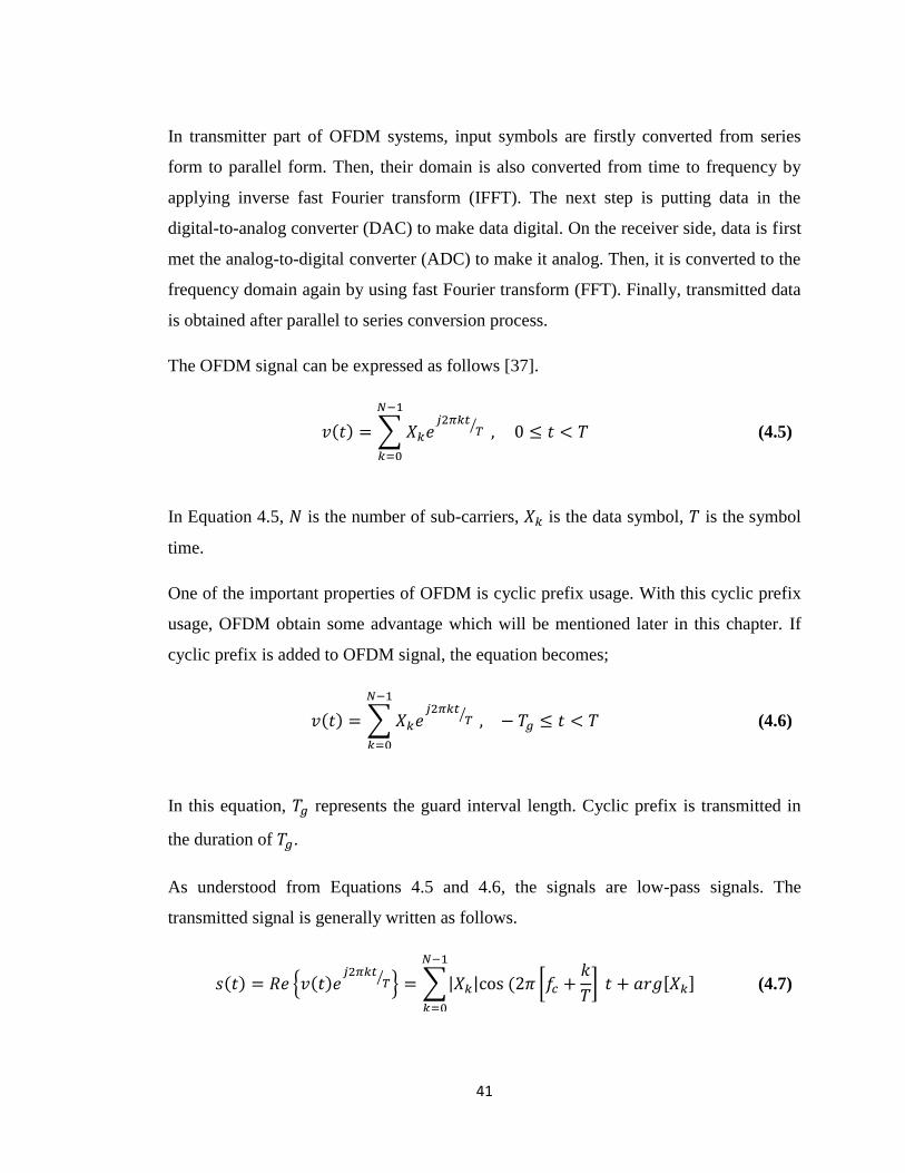
The OFDM signal can be expressed as follows [37].

(4.5)

In Equation 4.5, is the number of sub-carriers, is the data symbol, is the symbol

time.

One of the important properties of OFDM is cyclic prefix usage. With this cyclic prefix

usage, OFDM obtain some advantage which will be mentioned later in this chapter. If

cyclic prefix is added to OFDM signal, the equation becomes;

(4.6)

In this equation, represents the guard interval length. Cyclic prefix is transmitted in

the duration of .

As understood from Equations 4.5 and 4.6, the signals are low-pass signals. The

transmitted signal is generally written as follows.

(4.7)

42

In the Equation 4.7, general transmitted signal for OFDM is shown. is the carrier

frequency.

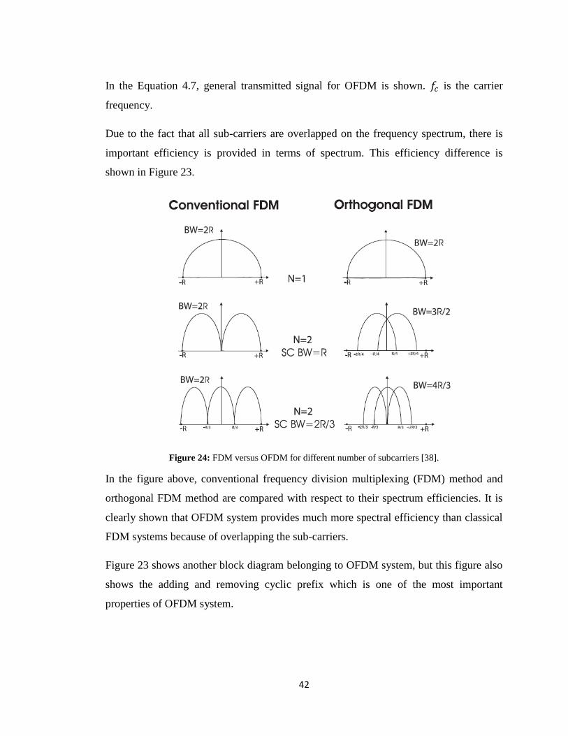
Due to the fact that all sub-carriers are overlapped on the frequency spectrum, there is

important efficiency is provided in terms of spectrum. This efficiency difference is

shown in Figure 23.

Figure 24: FDM versus OFDM for different number of subcarriers [38].

In the figure above, conventional frequency division multiplexing (FDM) method and

orthogonal FDM method are compared with respect to their spectrum efficiencies. It is

clearly shown that OFDM system provides much more spectral efficiency than classical

FDM systems because of overlapping the sub-carriers.

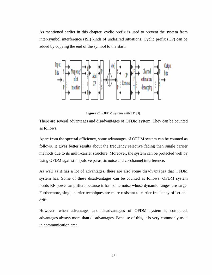
Figure 23 shows another block diagram belonging to OFDM system, but this figure also

shows the adding and removing cyclic prefix which is one of the most important

properties of OFDM system.

43

As mentioned earlier in this chapter, cyclic prefix is used to prevent the system from

inter-symbol interference (ISI) kinds of undesired situations. Cyclic prefix (CP) can be

added by copying the end of the symbol to the start.

Figure 25: OFDM system with CP [3].

There are several advantages and disadvantages of OFDM system. They can be counted

as follows.

Apart from the spectral efficiency, some advantages of OFDM system can be counted as

follows. It gives better results about the frequency selective fading than single carrier

methods due to its multi-carrier structure. Moreover, the system can be protected well by

using OFDM against impulsive parasitic noise and co-channel interference.

As well as it has a lot of advantages, there are also some disadvantages that OFDM

system has. Some of these disadvantages can be counted as follows. OFDM system

needs RF power amplifiers because it has some noise whose dynamic ranges are large.

Furthermore, single carrier techniques are more resistant to carrier frequency offset and

drift.

However, when advantages and disadvantages of OFDM system is compared,

advantages always more than disadvantages. Because of this, it is very commonly used

in communication area.

44

There are numerous application areas belonging to OFDM system such as digital radio

broadcasting, future mobile communication technologies; for instance 4G, WiMAX, and

ADSL.

4.1.3. Bit-Error Rate (BER) and Signal-to-Noise Ratio (SNR)

Bit-Error-Rate (BER) is very important concept for communication systems to specify

the system performance. It gives really important information about the quality of the

communication systems. Basically, BER is the ratio between the number of bit errors

and total number of bits that are transmitted within a certain time interval. This bit errors

occur because of some undesired parameters such as noise and interference.

As understood its definition, when the value of BER increases, system quality decreases.

In other words, higher BER value means lower system performance. Because of this

reason, the main focus for almost every communication systems is decreasing BER

value.

If Additional White Gaussian Noise (AWGN) is assumed for MQAM modulation

technique, BER can be calculated as follows.

(4.8)

where represents the energy per symbol. Then,

ratio can be written in terms of

ratio as follows.

(4.9)

where

represents energy per bit to noise power spectral density ratio.

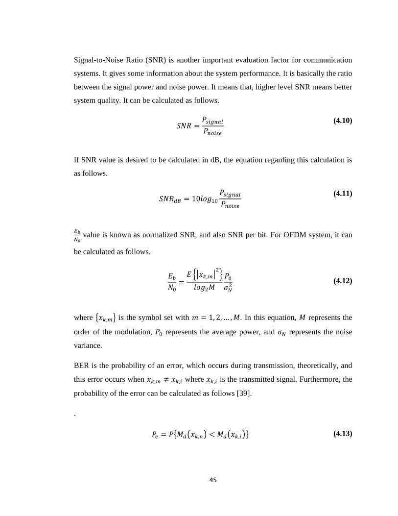
45

Signal-to-Noise Ratio (SNR) is another important evaluation factor for communication

systems. It gives some information about the system performance. It is basically the ratio

between the signal power and noise power. It means that, higher level SNR means better

system quality. It can be calculated as follows.

(4.10)

If SNR value is desired to be calculated in dB, the equation regarding this calculation is

as follows.

(4.11)

value is known as normalized SNR, and also SNR per bit. For OFDM system, it can

be calculated as follows.

(4.12)

where is the symbol set with . In this equation, represents the

order of the modulation, represents the average power, and represents the noise

variance.

BER is the probability of an error, which occurs during transmission, theoretically, and

this error occurs when where is the transmitted signal. Furthermore, the

probability of the error can be calculated as follows [39].

.

(4.13)

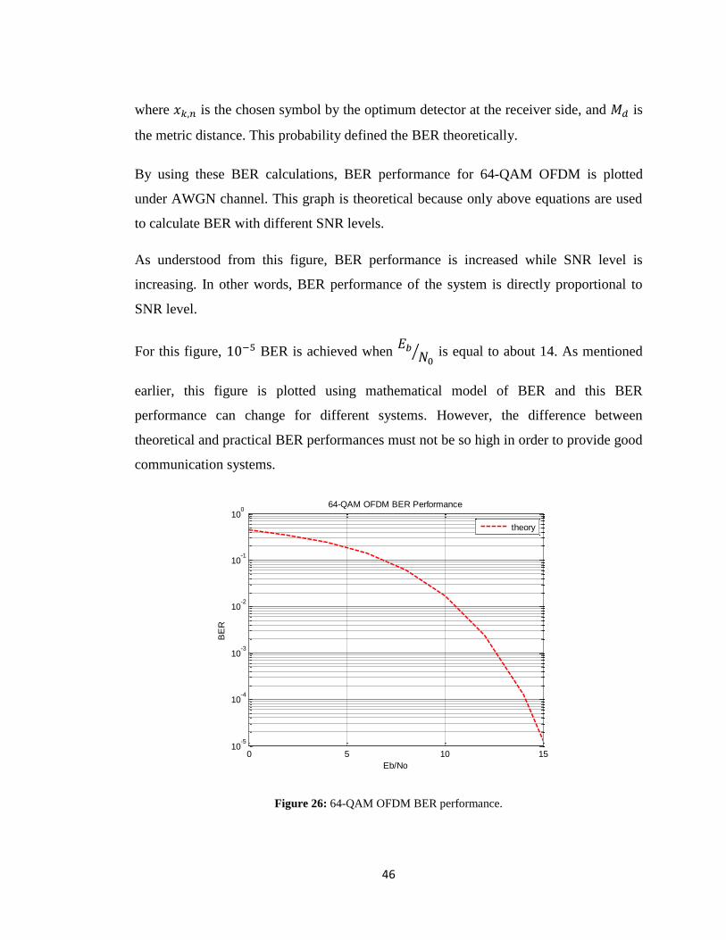
46

where is the chosen symbol by the optimum detector at the receiver side, and is

the metric distance. This probability defined the BER theoretically.

By using these BER calculations, BER performance for 64-QAM OFDM is plotted

under AWGN channel. This graph is theoretical because only above equations are used

to calculate BER with different SNR levels.

As understood from this figure, BER performance is increased while SNR level is

increasing. In other words, BER performance of the system is directly proportional to

SNR level.

For this figure, BER is achieved when

is equal to about 14. As mentioned

earlier, this figure is plotted using mathematical model of BER and this BER

performance can change for different systems. However, the difference between

theoretical and practical BER performances must not be so high in order to provide good

communication systems.

Figure 26: 64-QAM OFDM BER performance.

0 5 10 1510

-5

10-4

10-3

10-2

10-1

100

Eb/No

BE

R

64-QAM OFDM BER Performance

theory

47

4.1.4. Channel Coding

Channel coding, which is also called Forward Error Correction (FEC), is very important

for all digital communication systems because it allows to obtain less errors while data

transmission. There are lots of different coding techniques and they are based on

Shannon’s limit which states that the probability of error is small if channel capacity is

greater than the transmitted information. Otherwise, probability of error at the receiver is

not small [40].

Main advanced coding techniques are convolutional coding, Reed Solomon coding, and

turbo coding. In this part, these different advanced coding techniques are introduced

briefly.

4.1.4.1 Convolutional Coding

In convolutional coding, parity bits are generated using bits to be transmitted. Then, only

parity bits are transmitted over a communication channel instead of message bits. In

order to perform this process, window is sliding firstly to compute parity bits. In

addition to this, number of parity bits is greater than 1.

There are important parameters to specify the coding type which are number of input

bits ( ), number of output bits ( ), and number of memory register ( ). There is another

parameter in convolutional coding which is constraint length which represents the size

of window. Constraint length is calculated as follows.

(4.14)

Furthermore, the code rate can be calculated as where represents the number of

parity bits. There is also polynomial generator which is represented by . By using

message signal and polynomial generator, parity bits can be calculated as follows [38].

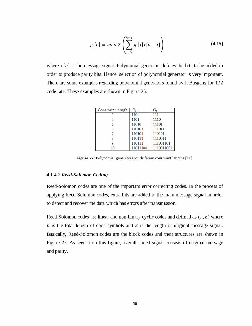
48

(4.15)

where is the message signal. Polynomial generator defines the bits to be added in

order to produce parity bits. Hence, selection of polynomial generator is very important.

There are some examples regarding polynomial generators found by J. Busgang for

code rate. These examples are shown in Figure 26.

Figure 27: Polynomial generators for different constraint lengths [41].

4.1.4.2 Reed-Solomon Coding

Reed-Solomon codes are one of the important error correcting codes. In the process of

applying Reed-Solomon codes, extra bits are added to the main message signal in order

to detect and recover the data which has errors after transmission.

Reed-Solomon codes are linear and non-binary cyclic codes and defined as where

is the total length of code symbols and is the length of original message signal.

Basically, Reed-Solomon codes are the block codes and their structures are shown in

Figure 27. As seen from this figure, overall coded signal consists of original message

and parity.

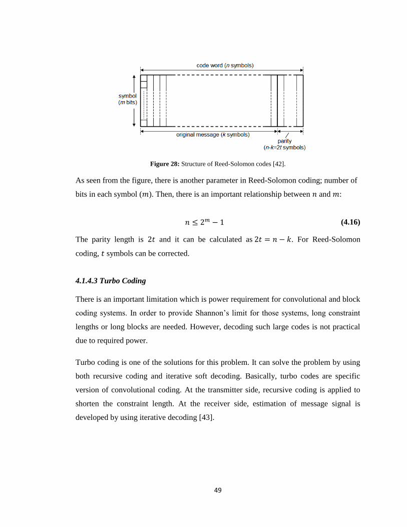
49

Figure 28: Structure of Reed-Solomon codes [42].

As seen from the figure, there is another parameter in Reed-Solomon coding; number of

bits in each symbol ( ). Then, there is an important relationship between and :

(4.16)

The parity length is and it can be calculated as . For Reed-Solomon

coding, symbols can be corrected.

4.1.4.3 Turbo Coding

There is an important limitation which is power requirement for convolutional and block

coding systems. In order to provide Shannon’s limit for those systems, long constraint

lengths or long blocks are needed. However, decoding such large codes is not practical

due to required power.

Turbo coding is one of the solutions for this problem. It can solve the problem by using

both recursive coding and iterative soft decoding. Basically, turbo codes are specific

version of convolutional coding. At the transmitter side, recursive coding is applied to

shorten the constraint length. At the receiver side, estimation of message signal is

developed by using iterative decoding [43].

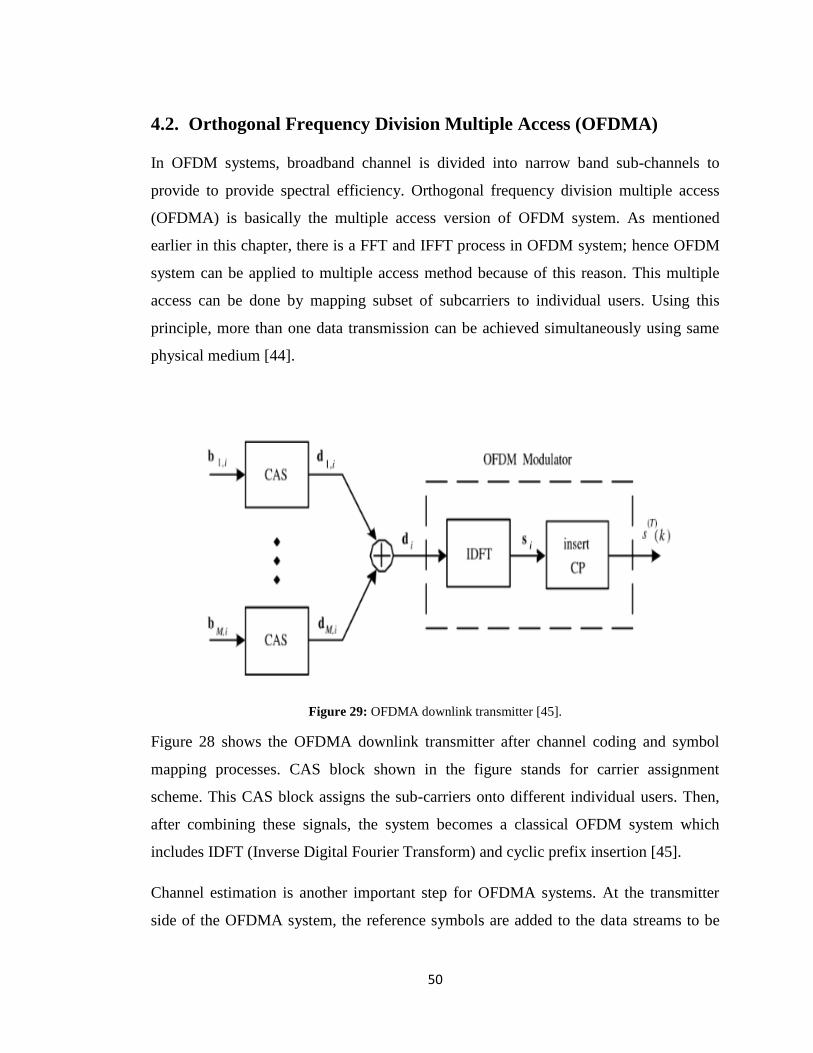
50

4.2. Orthogonal Frequency Division Multiple Access (OFDMA)

In OFDM systems, broadband channel is divided into narrow band sub-channels to

provide to provide spectral efficiency. Orthogonal frequency division multiple access

(OFDMA) is basically the multiple access version of OFDM system. As mentioned

earlier in this chapter, there is a FFT and IFFT process in OFDM system; hence OFDM

system can be applied to multiple access method because of this reason. This multiple

access can be done by mapping subset of subcarriers to individual users. Using this

principle, more than one data transmission can be achieved simultaneously using same

physical medium [44].

Figure 29: OFDMA downlink transmitter [45].

Figure 28 shows the OFDMA downlink transmitter after channel coding and symbol

mapping processes. CAS block shown in the figure stands for carrier assignment

scheme. This CAS block assigns the sub-carriers onto different individual users. Then,

after combining these signals, the system becomes a classical OFDM system which

includes IDFT (Inverse Digital Fourier Transform) and cyclic prefix insertion [45].

Channel estimation is another important step for OFDMA systems. At the transmitter

side of the OFDMA system, the reference symbols are added to the data streams to be

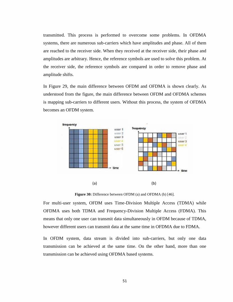
51

transmitted. This process is performed to overcome some problems. In OFDMA

systems, there are numerous sub-carriers which have amplitudes and phase. All of them

are reached to the receiver side. When they received at the receiver side, their phase and

amplitudes are arbitrary. Hence, the reference symbols are used to solve this problem. At

the receiver side, the reference symbols are compared in order to remove phase and

amplitude shifts.

In Figure 29, the main difference between OFDM and OFDMA is shown clearly. As

understood from the figure, the main difference between OFDM and OFDMA schemes

is mapping sub-carriers to different users. Without this process, the system of OFDMA

becomes an OFDM system.

(a) (b)

Figure 30: Difference between OFDM (a) and OFDMA (b) [46].

For multi-user system, OFDM uses Time-Division Multiple Access (TDMA) while

OFDMA uses both TDMA and Frequency-Division Multiple Access (FDMA). This

means that only one user can transmit data simultaneously in OFDM because of TDMA,

however different users can transmit data at the same time in OFDMA due to FDMA.

In OFDM system, data stream is divided into sub-carriers, but only one data

transmission can be achieved at the same time. On the other hand, more than one

transmission can be achieved using OFDMA based systems.

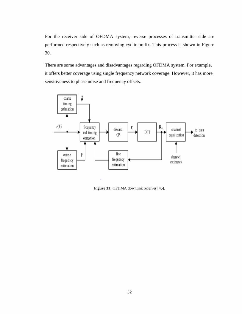
52

For the receiver side of OFDMA system, reverse processes of transmitter side are

performed respectively such as removing cyclic prefix. This process is shown in Figure

30.

There are some advantages and disadvantages regarding OFDMA system. For example,

it offers better coverage using single frequency network coverage. However, it has more

sensitiveness to phase noise and frequency offsets.

Figure 31: OFDMA downlink receiver [45].

53

CHAPTER FIVE

VLC SYSTEM DESIGN AND RESULTS

In this chapter, there are simulations studies regarding optical power distribution and

OFDM/OFDMA systems. These simulation studies are performed under various

conditions.

In optical power distribution part, the main focus is decreasing the dead zones which

occur in the receiver plane of communication area. Although the main purpose of the

optical power distribution study is dead zone minimization, there are some other studies

belonging to optical power. For instance, different conditions that affect the system

performances such as LED illumination angle, the distance between the transmitter and

receiver, and LED placements are also examined in this part.

Apart from these, other function is defined, which is called as uniformity function, to see

the uniformity of the optical power distribution under various conditions. Furthermore,

received minimum optical power and received maximum optical power are also

investigated. All these parameters will define the quality of the system performance.

Second study area is about the modulation technique. Orthogonal frequency division

multiplexing (OFDM) modulation technique, which is the most commonly used multi-

carrier modulation scheme, is studied, and this technique is applied to visible light

communication (VLC) systems. While applying OFDM system to visible light

communication system, quadrature amplitude modulation (QAM) technique is used, and

this system is called as M-QAM-OFDM visible light communication system. M value

defines the type of QAM method such as 4-QAM and 64-QAM. System performances

are examined for 64-QAM OFDM VLC.

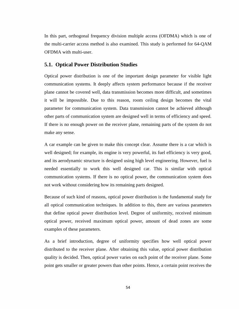
54

In this part, orthogonal frequency division multiple access (OFDMA) which is one of

the multi-carrier access method is also examined. This study is performed for 64-QAM

OFDMA with multi-user.

5.1. Optical Power Distribution Studies

Optical power distribution is one of the important design parameter for visible light

communication systems. It deeply affects system performance because if the receiver

plane cannot be covered well, data transmission becomes more difficult, and sometimes

it will be impossible. Due to this reason, room ceiling design becomes the vital

parameter for communication system. Data transmission cannot be achieved although

other parts of communication system are designed well in terms of efficiency and speed.

If there is no enough power on the receiver plane, remaining parts of the system do not

make any sense.

A car example can be given to make this concept clear. Assume there is a car which is

well designed; for example, its engine is very powerful, its fuel efficiency is very good,

and its aerodynamic structure is designed using high level engineering. However, fuel is

needed essentially to work this well designed car. This is similar with optical

communication systems. If there is no optical power, the communication system does

not work without considering how its remaining parts designed.

Because of such kind of reasons, optical power distribution is the fundamental study for

all optical communication techniques. In addition to this, there are various parameters

that define optical power distribution level. Degree of uniformity, received minimum

optical power, received maximum optical power, amount of dead zones are some

examples of these parameters.

As a brief introduction, degree of uniformity specifies how well optical power

distributed to the receiver plane. After obtaining this value, optical power distribution

quality is decided. Then, optical power varies on each point of the receiver plane. Some

point gets smaller or greater powers than other points. Hence, a certain point receives the

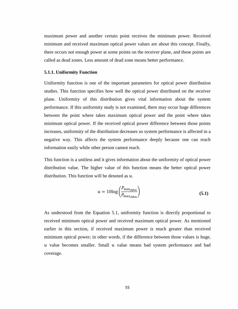
55

maximum power and another certain point receives the minimum power. Received

minimum and received maximum optical power values are about this concept. Finally,

there occurs not enough power at some points on the receiver plane, and these points are

called as dead zones. Less amount of dead zone means better performance.

5.1.1. Uniformity Function

Uniformity function is one of the important parameters for optical power distribution

studies. This function specifies how well the optical power distributed on the receiver

plane. Uniformity of this distribution gives vital information about the system

performance. If this uniformity study is not examined, there may occur huge differences

between the point where takes maximum optical power and the point where takes

minimum optical power. If the received optical power difference between those points

increases, uniformity of the distribution decreases so system performance is affected in a

negative way. This affects the system performance deeply because one can reach

information easily while other person cannot reach.

This function is a unitless and it gives information about the uniformity of optical power

distribution value. The higher value of this function means the better optical power

distribution. This function will be denoted as .

(5.1)

As understood from the Equation 5.1, uniformity function is directly proportional to

received minimum optical power and received maximum optical power. As mentioned

earlier in this section, if received maximum power is much greater than received

minimum optical power; in other words, if the difference between those values is huge,

value becomes smaller. Small value means bad system performance and bad

coverage.

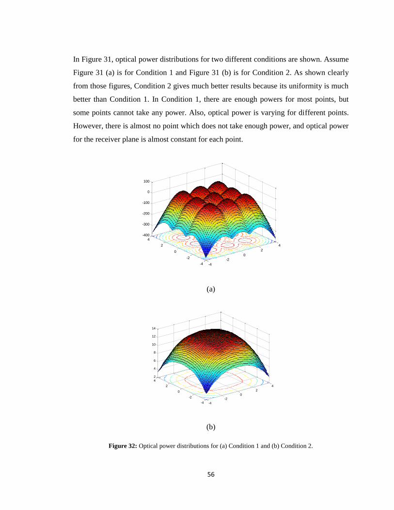
56

In Figure 31, optical power distributions for two different conditions are shown. Assume

Figure 31 (a) is for Condition 1 and Figure 31 (b) is for Condition 2. As shown clearly

from those figures, Condition 2 gives much better results because its uniformity is much

better than Condition 1. In Condition 1, there are enough powers for most points, but

some points cannot take any power. Also, optical power is varying for different points.

However, there is almost no point which does not take enough power, and optical power

for the receiver plane is almost constant for each point.

(a)

(b)

Figure 32: Optical power distributions for (a) Condition 1 and (b) Condition 2.

-4

-2

0

2

4

-4

-2

0

2

4-400

-300

-200

-100

0

100

-4

-2

0

2

4

-4

-2

0

2

42

4

6

8

10

12

14

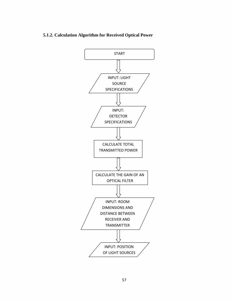
57

5.1.2. Calculation Algorithm for Received Optical Power

START

CALCULATE TOTAL

TRANSMITTED POWER

CALCULATE THE GAIN OF AN

OPTICAL FILTER

INPUT: LIGHT

SOURCE

SPECIFICATIONS

INPUT:

DETECTOR

SPECIFICATIONS

INPUT: ROOM

DIMENSIONS AND

DISTANCE BETWEEN

RECEIVER AND

TRANSMITTER

INPUT: POSITION

OF LIGHT SOURCES

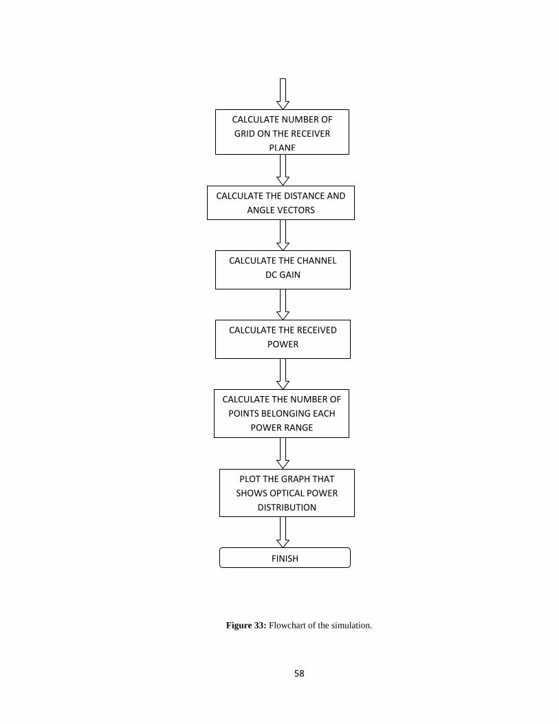
58

Figure 33: Flowchart of the simulation.

CALCULATE NUMBER OF

GRID ON THE RECEIVER

PLANE

CALCULATE THE DISTANCE AND

ANGLE VECTORS

CALCULATE THE CHANNEL

DC GAIN

CALCULATE THE RECEIVED

POWER

CALCULATE THE NUMBER OF

POINTS BELONGING EACH

POWER RANGE

PLOT THE GRAPH THAT

SHOWS OPTICAL POWER

DISTRIBUTION

FINISH

59

5.1.3. Transmitter and Receiver Specifications

Cree Company’s CP41B-WES series LEDs are used in this study. Specifications

regarding these LEDs are given in Table 1.

Table 1: Specifications of CP41B-WES.

Parameter Value

Forward Current

Peak Forward Current

Reverse Voltage

Power Dissipation

Luminous Flux

Luminous Intensity

50% Power Angle

Photo-detector specifications which are given in [3] are used in this study. These

specifications are given in the table below.

Table 2: Photo-detector specifications.

Parameter Value

Active Area

Half Angle FOV

Elevation

Azimuth

All these LED and photo-detector specifications are used in the simulation model. These

parameters are the inputs that are written on the flow chart which is given in the

previous section. After deciding which light source and which detector is used, received

optical power can be calculated easily.

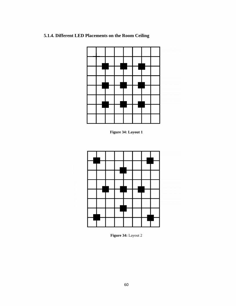
60

5.1.4. Different LED Placements on the Room Ceiling

Figure 34: Layout 1

Figure 34: Layout 2

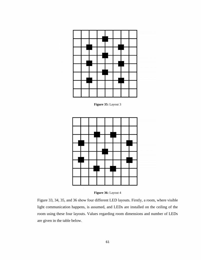
61

Figure 35: Layout 3

Figure 36: Layout 4

Figure 33, 34, 35, and 36 show four different LED layouts. Firstly, a room, where visible

light communication happens, is assumed, and LEDs are installed on the ceiling of the

room using these four layouts. Values regarding room dimensions and number of LEDs

are given in the table below.

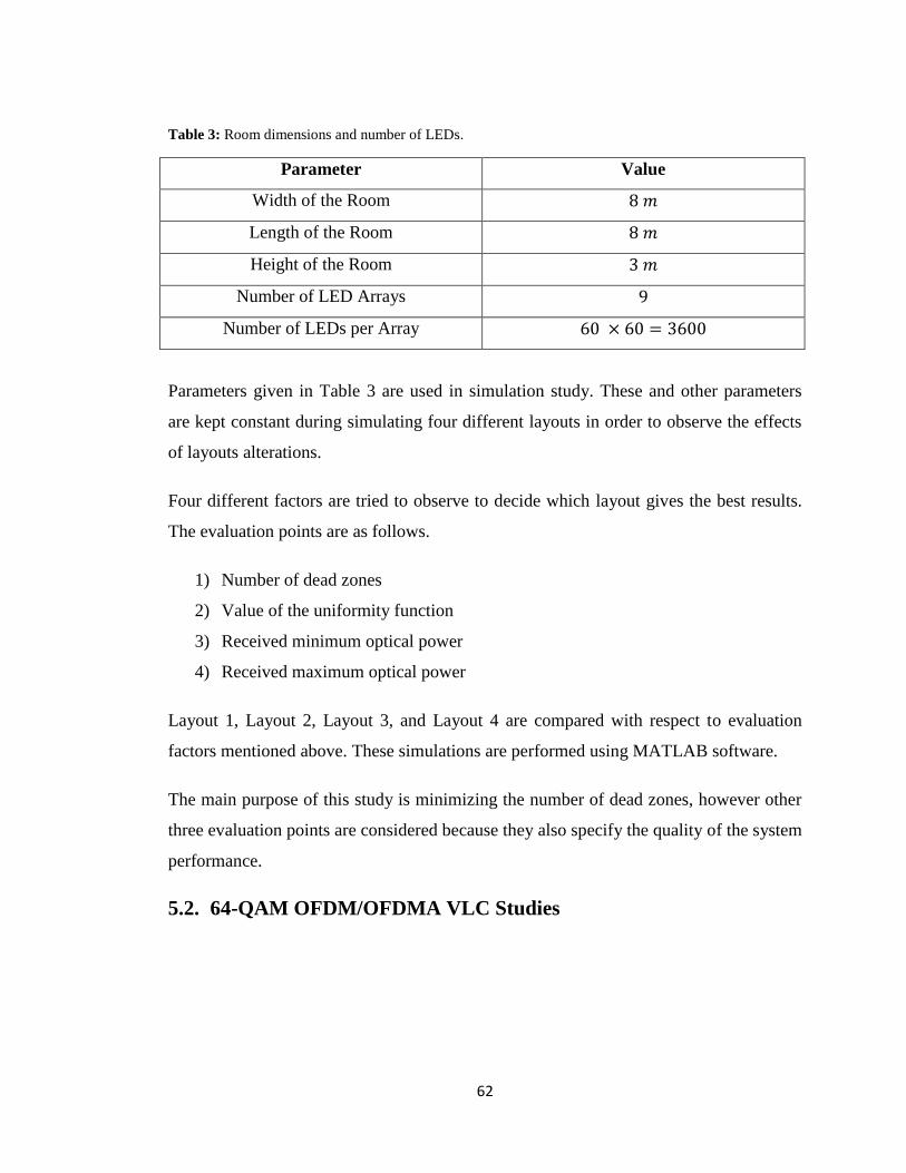
62

Table 3: Room dimensions and number of LEDs.

Parameter Value

Width of the Room

Length of the Room

Height of the Room

Number of LED Arrays

Number of LEDs per Array

Parameters given in Table 3 are used in simulation study. These and other parameters

are kept constant during simulating four different layouts in order to observe the effects

of layouts alterations.

Four different factors are tried to observe to decide which layout gives the best results.

The evaluation points are as follows.

1) Number of dead zones

2) Value of the uniformity function

3) Received minimum optical power

4) Received maximum optical power

Layout 1, Layout 2, Layout 3, and Layout 4 are compared with respect to evaluation

factors mentioned above. These simulations are performed using MATLAB software.

The main purpose of this study is minimizing the number of dead zones, however other

three evaluation points are considered because they also specify the quality of the system

performance.

5.2. 64-QAM OFDM/OFDMA VLC Studies

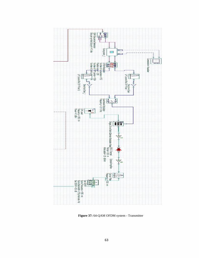
63

Figure 37: 64-QAM OFDM system - Transmitter

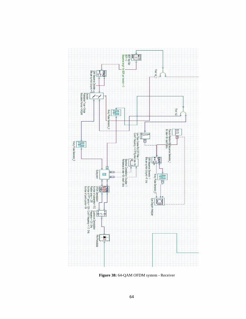
64

Figure 38: 64-QAM OFDM system - Receiver

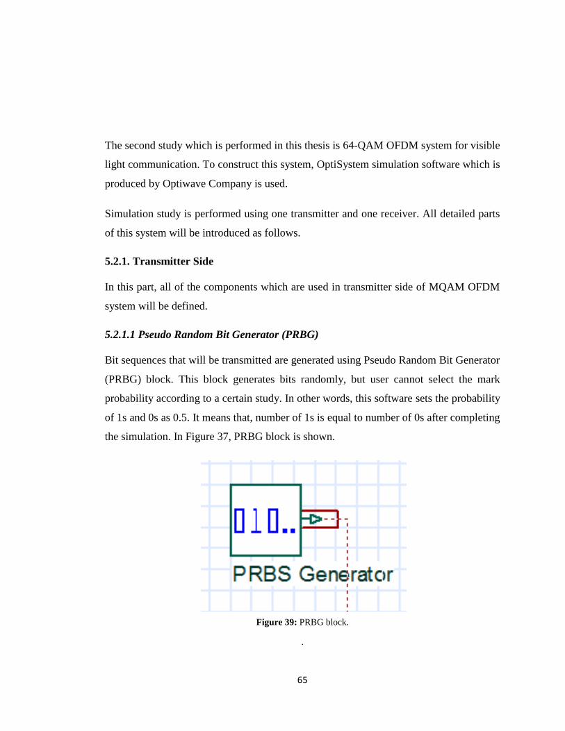
65

The second study which is performed in this thesis is 64-QAM OFDM system for visible

light communication. To construct this system, OptiSystem simulation software which is

produced by Optiwave Company is used.

Simulation study is performed using one transmitter and one receiver. All detailed parts

of this system will be introduced as follows.

5.2.1. Transmitter Side

In this part, all of the components which are used in transmitter side of MQAM OFDM

system will be defined.

5.2.1.1 Pseudo Random Bit Generator (PRBG)

Bit sequences that will be transmitted are generated using Pseudo Random Bit Generator

(PRBG) block. This block generates bits randomly, but user cannot select the mark

probability according to a certain study. In other words, this software sets the probability

of 1s and 0s as 0.5. It means that, number of 1s is equal to number of 0s after completing

the simulation. In Figure 37, PRBG block is shown.

Figure 39: PRBG block.

.

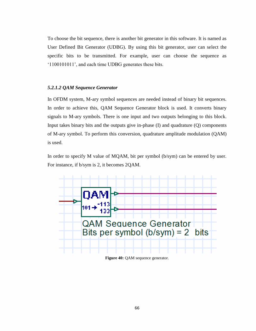
66

To choose the bit sequence, there is another bit generator in this software. It is named as

User Defined Bit Generator (UDBG). By using this bit generator, user can select the

specific bits to be transmitted. For example, user can choose the sequence as

‘1100101011’, and each time UDBG generates these bits.

5.2.1.2 QAM Sequence Generator

In OFDM system, M-ary symbol sequences are needed instead of binary bit sequences.

In order to achieve this, QAM Sequence Generator block is used. It converts binary

signals to M-ary symbols. There is one input and two outputs belonging to this block.

Input takes binary bits and the outputs give in-phase (I) and quadrature (Q) components

of M-ary symbol. To perform this conversion, quadrature amplitude modulation (QAM)

is used.

In order to specify M value of MQAM, bit per symbol (b/sym) can be entered by user.

For instance, if b/sym is 2, it becomes 2QAM.

Figure 40: QAM sequence generator.

67

5.2.1.3 OFDM Modulator

This block is one of the most important blocks in this simulation system because OFDM

modulation is performed in this block. M-ary symbols which are generated by QAM

Sequence generator block become input for OFDM Modulator. This block takes those

M-ary signals and converts them into orthogonal sub-carriers. It has two inputs and two

outputs. While input signals are M-ary, output signals are electrical signals. Similarly,

the output signal consists of in-phase (I) and quadrature (Q) components.

Table 4: OFDM Modulator parameters.

Parameter Value

Number of Sub-Carriers

Position Array

Number of FFT points

Cyclic Prefix

Parameters which are used in OFDM Modulator is given in Table 4.

5.2.1.4 Low-Pass Cosine Roll Off Filter

There is a filter used in transmitter part of the overall system. This filter is known as

Low-Pass (LP) Cosine Roll Off Filter. This filter applies the cosine roll off frequency

transfer function to incoming electrical signal, and then gives filtered electrical output.

The frequencies between the certain frequencies, which are and , can pass from this

filter. This frequencies are calculated as follows.

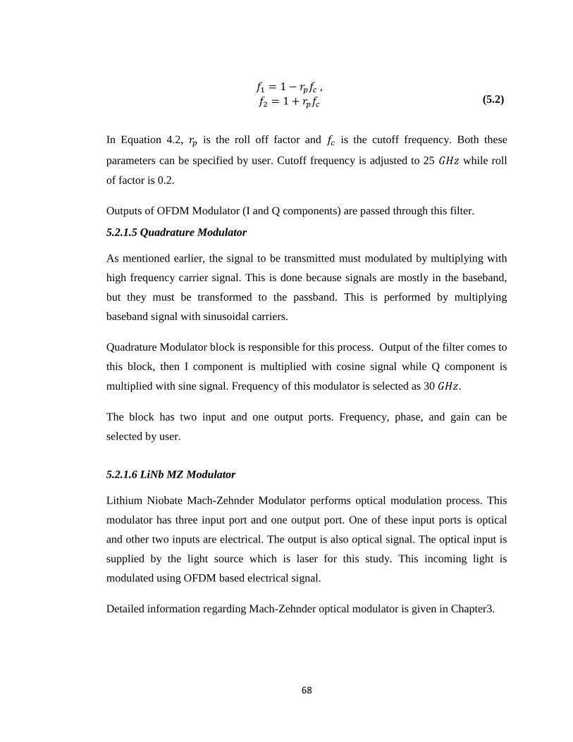
68

,

(5.2)

In Equation 4.2, is the roll off factor and is the cutoff frequency. Both these

parameters can be specified by user. Cutoff frequency is adjusted to 25 while roll

of factor is 0.2.

Outputs of OFDM Modulator (I and Q components) are passed through this filter.

5.2.1.5 Quadrature Modulator

As mentioned earlier, the signal to be transmitted must modulated by multiplying with

high frequency carrier signal. This is done because signals are mostly in the baseband,

but they must be transformed to the passband. This is performed by multiplying

baseband signal with sinusoidal carriers.

Quadrature Modulator block is responsible for this process. Output of the filter comes to

this block, then I component is multiplied with cosine signal while Q component is

multiplied with sine signal. Frequency of this modulator is selected as 30 .

The block has two input and one output ports. Frequency, phase, and gain can be

selected by user.

5.2.1.6 LiNb MZ Modulator

Lithium Niobate Mach-Zehnder Modulator performs optical modulation process. This

modulator has three input port and one output port. One of these input ports is optical

and other two inputs are electrical. The output is also optical signal. The optical input is

supplied by the light source which is laser for this study. This incoming light is

modulated using OFDM based electrical signal.

Detailed information regarding Mach-Zehnder optical modulator is given in Chapter3.

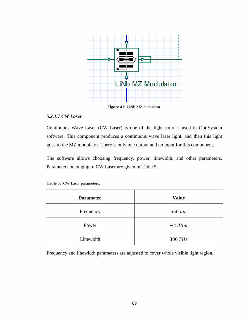
69

Figure 41: LiNb MZ modulator.

5.2.1.7 CW Laser

Continuous Wave Laser (CW Laser) is one of the light sources used in OptiSystem

software. This component produces a continuous wave laser light, and then this light

goes to the MZ modulator. There is only one output and no input for this component.

The software allows choosing frequency, power, linewidth, and other parameters.

Parameters belonging to CW Laser are given in Table 5.

Table 5: CW Laser parameters.

Parameter Value

Frequency

Power

Linewidth

Frequency and linewidth parameters are adjusted to cover whole visible light region.

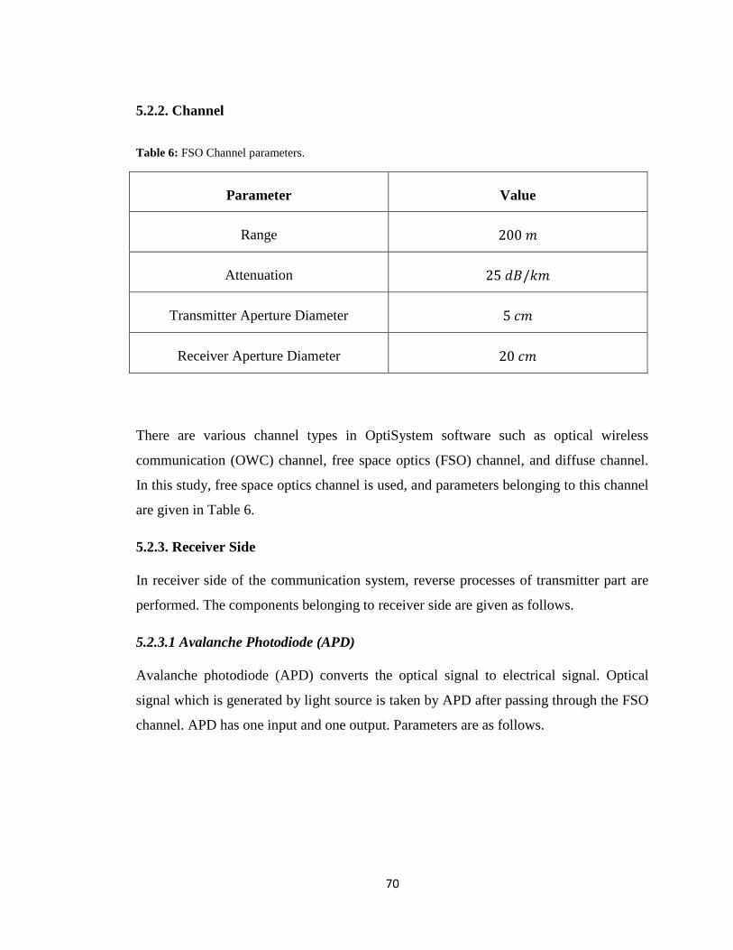
70

5.2.2. Channel

Table 6: FSO Channel parameters.

Parameter Value

Range

Attenuation

Transmitter Aperture Diameter

Receiver Aperture Diameter

There are various channel types in OptiSystem software such as optical wireless

communication (OWC) channel, free space optics (FSO) channel, and diffuse channel.

In this study, free space optics channel is used, and parameters belonging to this channel

are given in Table 6.

5.2.3. Receiver Side

In receiver side of the communication system, reverse processes of transmitter part are

performed. The components belonging to receiver side are given as follows.

5.2.3.1 Avalanche Photodiode (APD)

Avalanche photodiode (APD) converts the optical signal to electrical signal. Optical

signal which is generated by light source is taken by APD after passing through the FSO

channel. APD has one input and one output. Parameters are as follows.

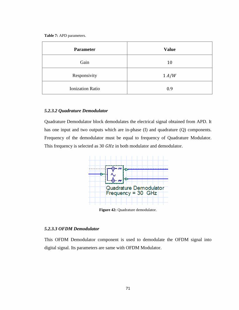
71

Table 7: APD parameters.

Parameter Value

Gain

Responsivity

Ionization Ratio

5.2.3.2 Quadrature Demodulator

Quadrature Demodulator block demodulates the electrical signal obtained from APD. It

has one input and two outputs which are in-phase (I) and quadrature (Q) components.

Frequency of the demodulator must be equal to frequency of Quadrature Modulator.

This frequency is selected as 30 in both modulator and demodulator.

Figure 42: Quadrature demodulator.

5.2.3.3 OFDM Demodulator

This OFDM Demodulator component is used to demodulate the OFDM signal into

digital signal. Its parameters are same with OFDM Modulator.

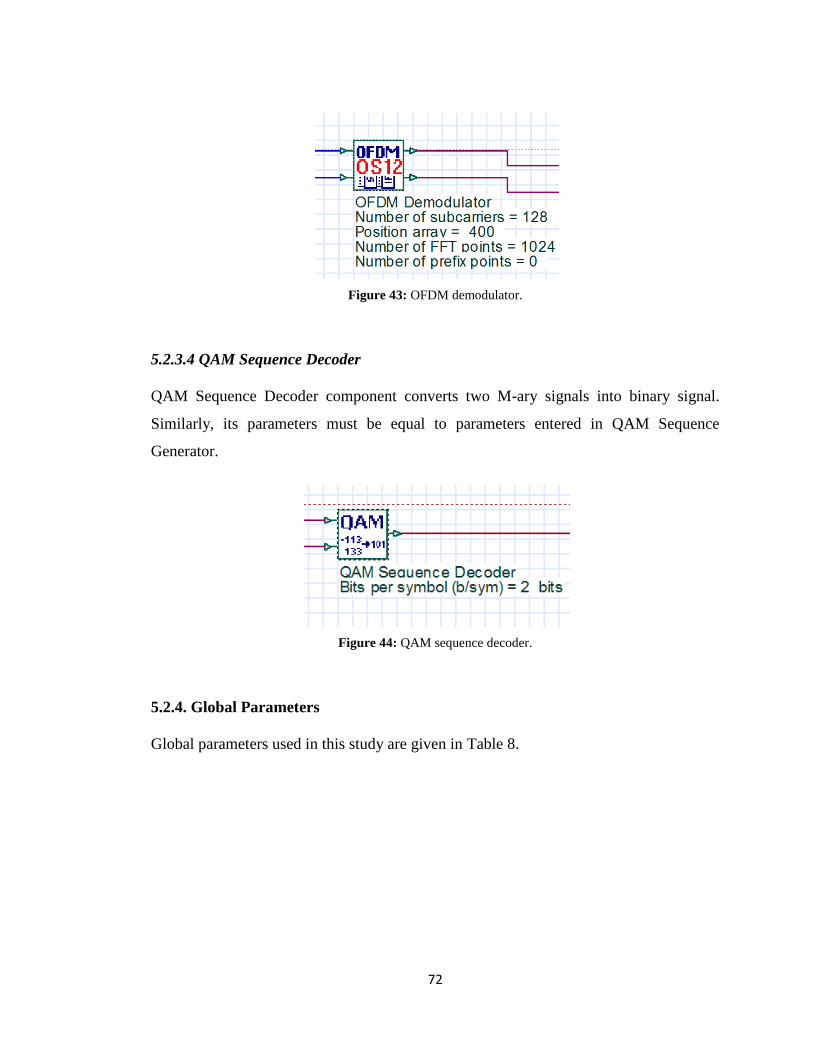
72

Figure 43: OFDM demodulator.

5.2.3.4 QAM Sequence Decoder

QAM Sequence Decoder component converts two M-ary signals into binary signal.

Similarly, its parameters must be equal to parameters entered in QAM Sequence

Generator.

Figure 44: QAM sequence decoder.

5.2.4. Global Parameters

Global parameters used in this study are given in Table 8.

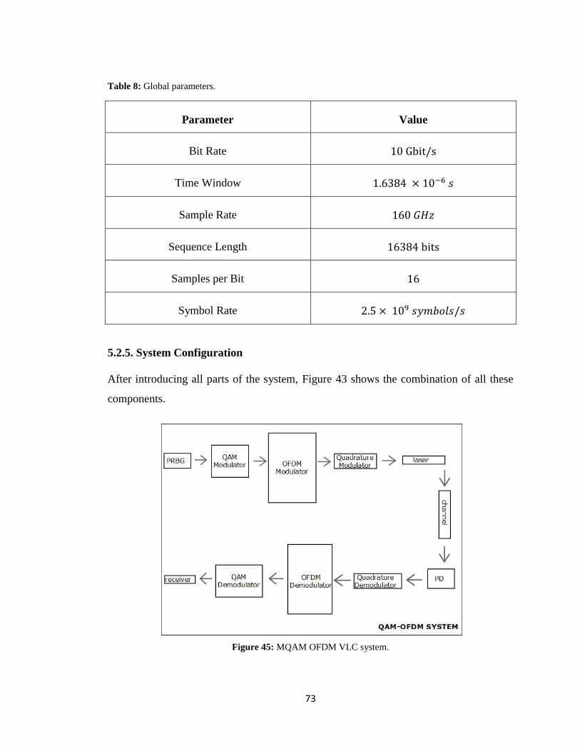
73

Table 8: Global parameters.

Parameter Value

Bit Rate

Time Window

Sample Rate

Sequence Length

Samples per Bit

Symbol Rate

5.2.5. System Configuration

After introducing all parts of the system, Figure 43 shows the combination of all these

components.

Figure 45: MQAM OFDM VLC system.

74

5.2.6. Proposed System

The following studies are performed in this thesis, respectively.

- 64-QAM OFDM system is constructed.

- 64-QAM OFDM systems are simulated.

- Results are analyzed and compared.

- 64-QAM OFDMA system is constructed.

- System is simulated for different number of users.

- Results belonging to 64-QAM OFDMA system are obtained.

- These results are compared in terms of the system performances.

75

5.3. Results and Discussions

In this chapter, obtained results including optical power distribution, MQAM OFDM

VLC system, and MQAM OFDMA VLC system are given, respectively.

First study is about optical power distribution. In this study, four different LED

placements are simulated in terms of their distribution performances. These four

different LED placements are named as Layout 1, Layout 2, Layout 3, and Layout 4.

The evaluation parameters are given in Chapter 4; received minimum optical power,

received maximum optical power, degree of uniformity, and number of dead zones. In

this part, there are results about these parameters.

Second study is about the MQAM OFDM visible light communication system. Different

MQAM OFDM VLC systems are constructed by changing M value. After constructing

4QAM OFDM, 16QAM OFDM, and 64QAM OFDM systems for visible light

communication systems, their system performances are investigated. After that,

comparisons regarding their performances are done in order to observe the effect of M

value.

The third study is about MQAM OFDMA visible light communication systems. As

mentioned earlier, OFDMA is the multi-user version of OFDM. For this study, different

number of users is assumed, and effects of number of users are investigated.

For optical power distribution study, MATLAB software is used to perform the

simulations. For MQAM OFDM VLC and MQAM OFDMA VLC systems, OptiSystem

simulation platform is used.

In Graphs 1, 2, 3, and 4, optical power distribution performances of all layouts are

shown clearly. 5 dB is selected as a threshold value, and the points that are received

powers under 5 dB is named as dead zone.

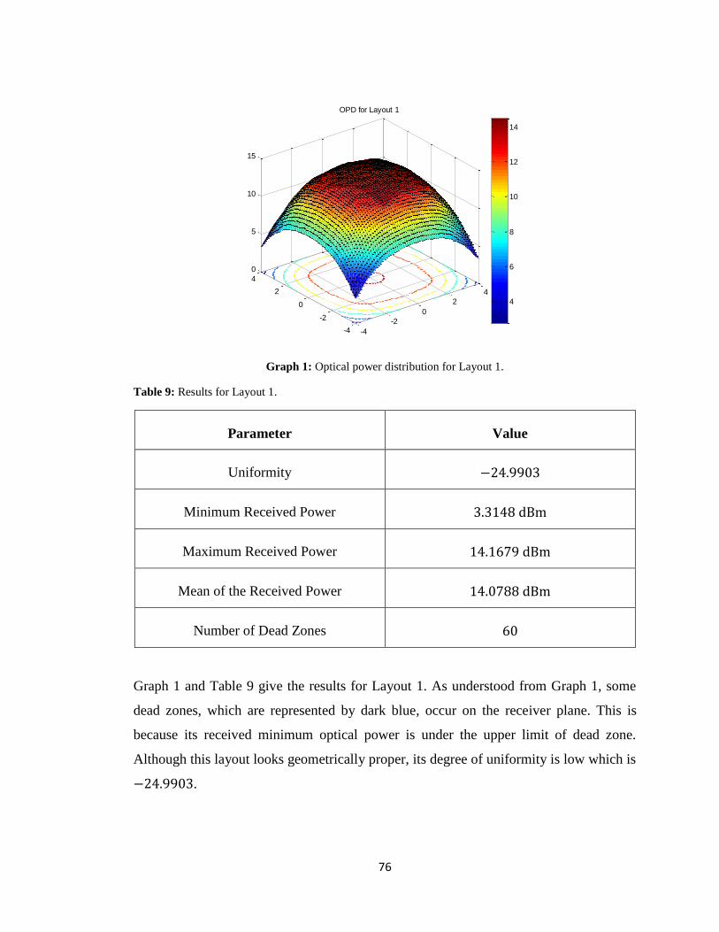
76

Graph 1: Optical power distribution for Layout 1.

Table 9: Results for Layout 1.

Parameter Value

Uniformity

Minimum Received Power

Maximum Received Power

Mean of the Received Power

Number of Dead Zones

Graph 1 and Table 9 give the results for Layout 1. As understood from Graph 1, some

dead zones, which are represented by dark blue, occur on the receiver plane. This is

because its received minimum optical power is under the upper limit of dead zone.

Although this layout looks geometrically proper, its degree of uniformity is low which is

24.9903.

-4

-2

0

2

4

-4

-2

0

2

4

0

5

10

15

OPD for Layout 1

4

6

8

10

12

14

77

Graph 2: Optical power distribution for Layout 2.

Table 10: Results for Layout 2.

Parameter Value

Uniformity

Minimum Received Power

Maximum Received Power

Mean of the Received Power

Number of Dead Zones

Graph 2 and Table 10 show results for Layout 2. From Graph 2, there is no dark blue

points on the receiver place. This means that no dead zones occurs. In other words, dead

zones of Layout 1 are minimized by changing the LED placements. Also, degree of

uniformity is improved from to ; it almost doubles. There is

another good improvement in Layout 2 when it is compared to Layout 1: received

minimum optical power. However, Layout 1’s received maximum optical power and

-4

-2

0

2

4

-4

-2

0

2

46

8

10

12

14

OPD for Layout 2

4

6

8

10

12

14

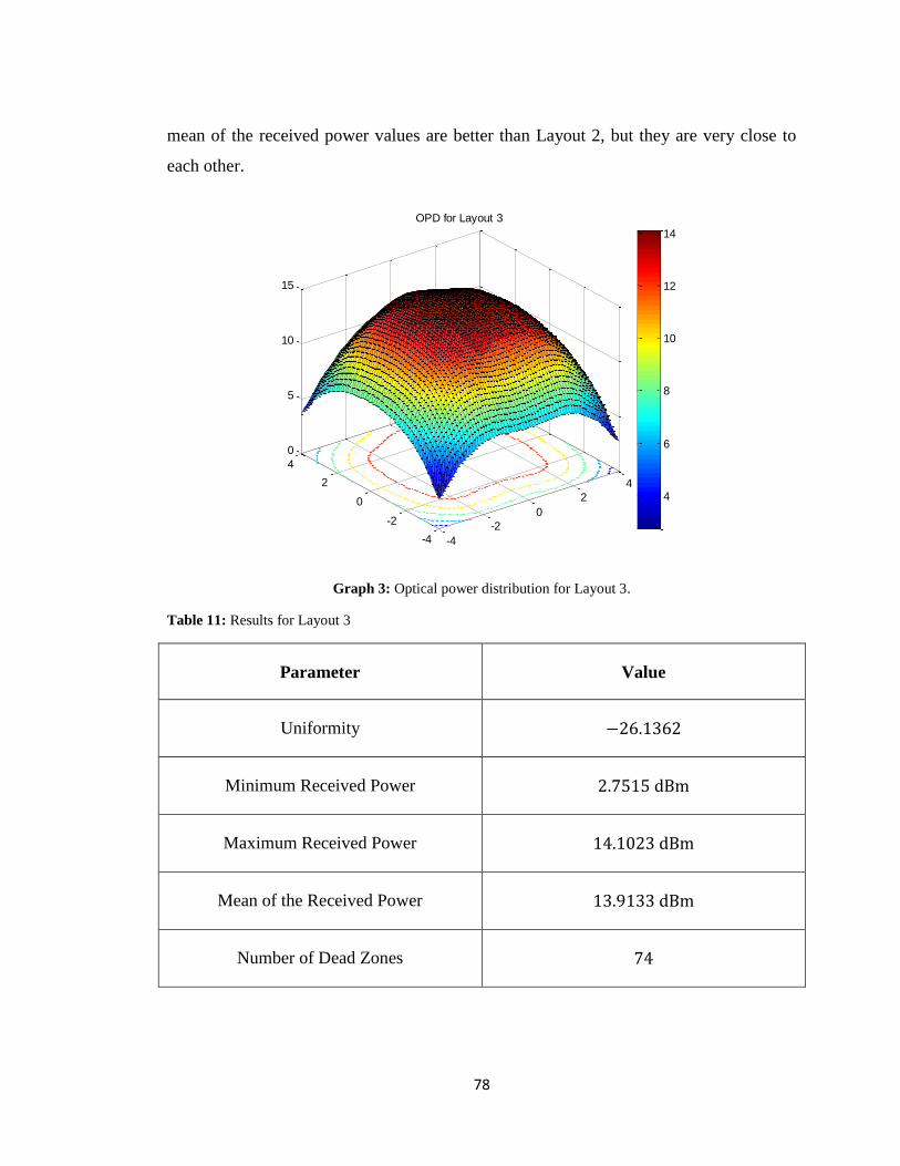
78

mean of the received power values are better than Layout 2, but they are very close to

each other.

Graph 3: Optical power distribution for Layout 3.

Table 11: Results for Layout 3

Parameter Value

Uniformity

Minimum Received Power

Maximum Received Power

Mean of the Received Power

Number of Dead Zones

-4

-2

0

2

4

-4

-2

0

2

4

0

5

10

15

OPD for Layout 3

4

6

8

10

12

14

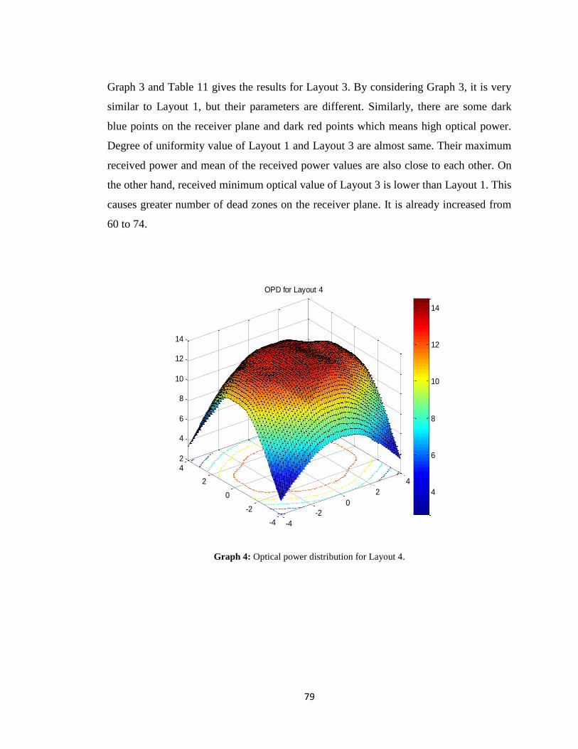
79

Graph 3 and Table 11 gives the results for Layout 3. By considering Graph 3, it is very

similar to Layout 1, but their parameters are different. Similarly, there are some dark

blue points on the receiver plane and dark red points which means high optical power.

Degree of uniformity value of Layout 1 and Layout 3 are almost same. Their maximum

received power and mean of the received power values are also close to each other. On

the other hand, received minimum optical value of Layout 3 is lower than Layout 1. This

causes greater number of dead zones on the receiver plane. It is already increased from

60 to 74.

Graph 4: Optical power distribution for Layout 4.

-4

-2

0

2

4

-4

-2

0

2

42

4

6

8

10

12

14

OPD for Layout 4

4

6

8

10

12

14

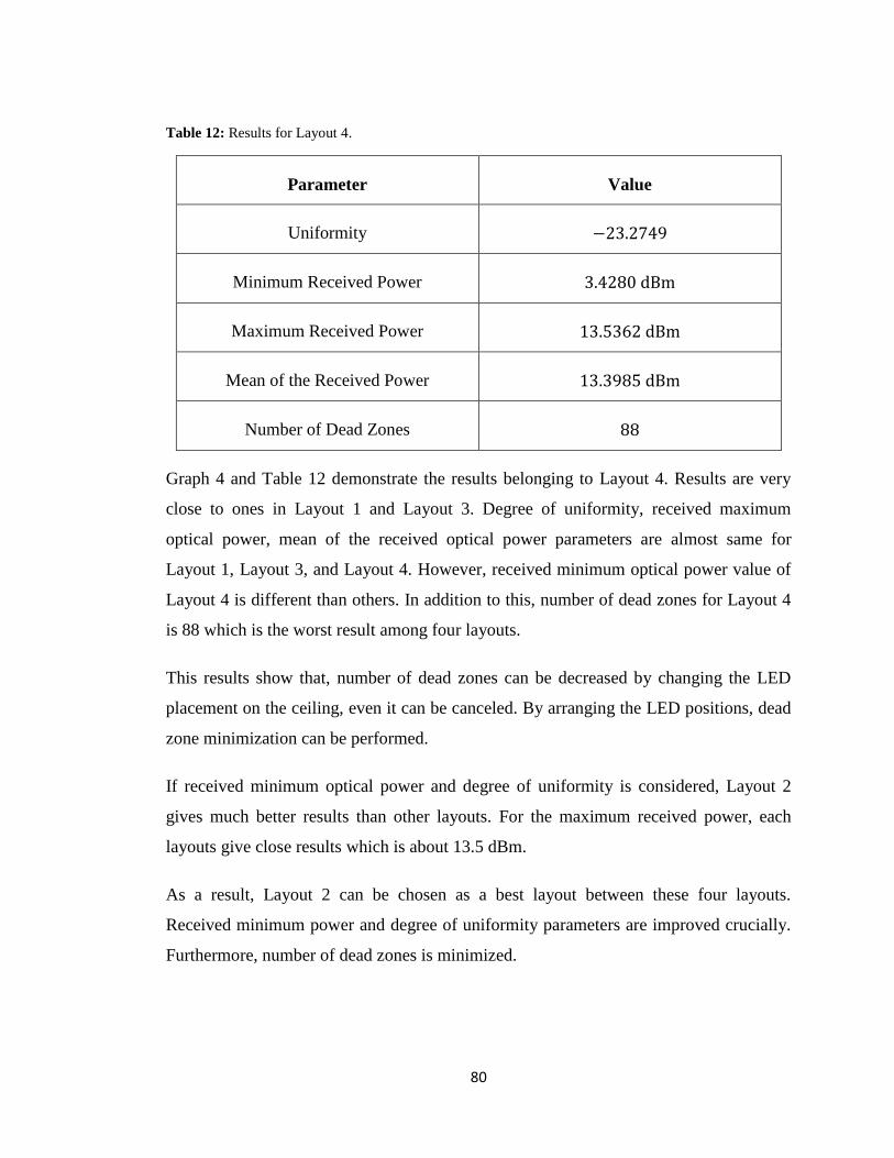
80

Table 12: Results for Layout 4.

Parameter Value

Uniformity

Minimum Received Power

Maximum Received Power

Mean of the Received Power

Number of Dead Zones

Graph 4 and Table 12 demonstrate the results belonging to Layout 4. Results are very

close to ones in Layout 1 and Layout 3. Degree of uniformity, received maximum

optical power, mean of the received optical power parameters are almost same for

Layout 1, Layout 3, and Layout 4. However, received minimum optical power value of

Layout 4 is different than others. In addition to this, number of dead zones for Layout 4

is 88 which is the worst result among four layouts.

This results show that, number of dead zones can be decreased by changing the LED

placement on the ceiling, even it can be canceled. By arranging the LED positions, dead

zone minimization can be performed.

If received minimum optical power and degree of uniformity is considered, Layout 2

gives much better results than other layouts. For the maximum received power, each

layouts give close results which is about 13.5 dBm.

As a result, Layout 2 can be chosen as a best layout between these four layouts.

Received minimum power and degree of uniformity parameters are improved crucially.

Furthermore, number of dead zones is minimized.

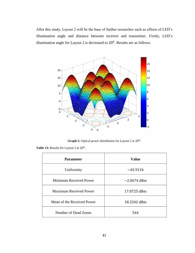
81

After this study, Layout 2 will be the base of further researches such as effects of LED’s

illumination angle and distance between receiver and transmitter. Firstly, LED’s

illumination angle for Layout 2 is decreased to . Results are as follows.

Graph 5: Optical power distribution for Layout 2 at .

Table 13: Results for Layout 2 at .

Parameter Value

Uniformity

Minimum Received Power

Maximum Received Power

Mean of the Received Power

Number of Dead Zones

-4

-2

0

2

4

-4

-2

0

2

4-5

0

5

10

15

20

-2

0

2

4

6

8

10

12

14

16

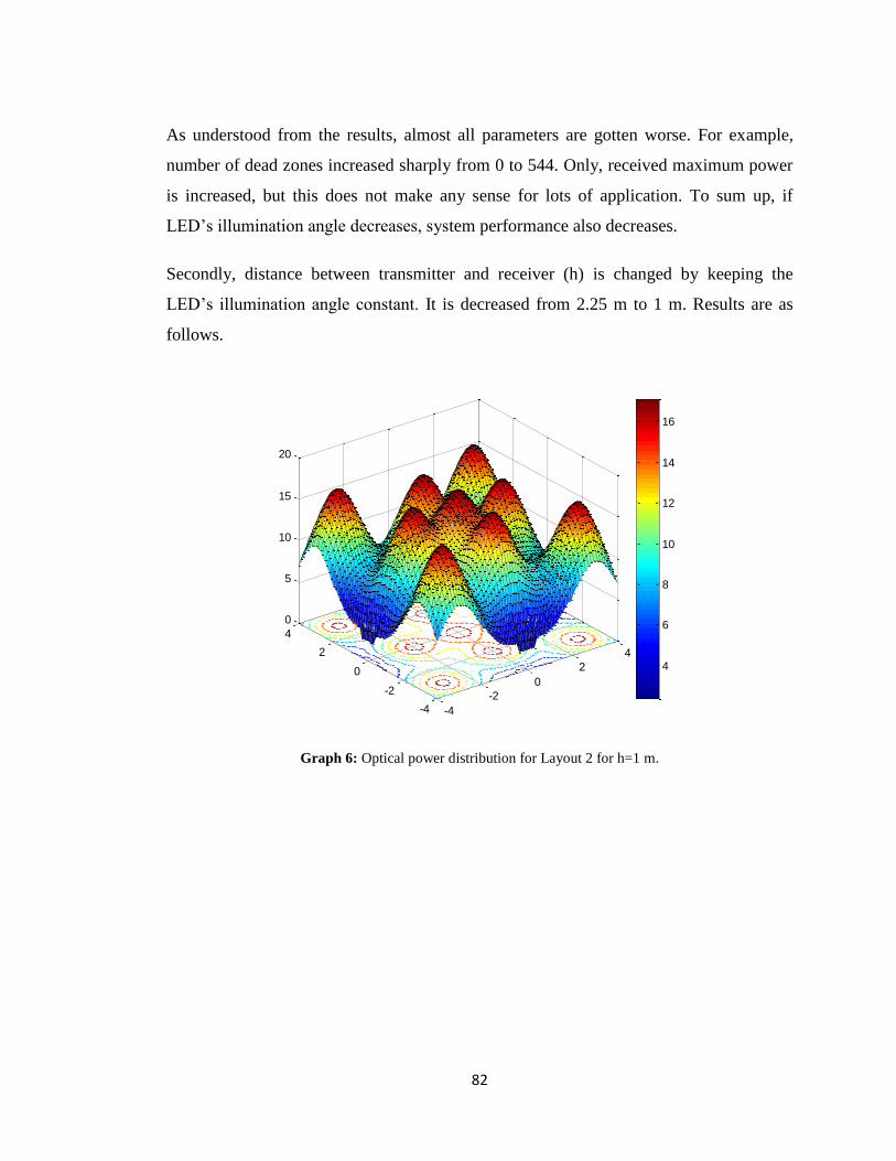
82

As understood from the results, almost all parameters are gotten worse. For example,

number of dead zones increased sharply from 0 to 544. Only, received maximum power

is increased, but this does not make any sense for lots of application. To sum up, if

LED’s illumination angle decreases, system performance also decreases.

Secondly, distance between transmitter and receiver (h) is changed by keeping the

LED’s illumination angle constant. It is decreased from 2.25 m to 1 m. Results are as

follows.

Graph 6: Optical power distribution for Layout 2 for h=1 m.

-4

-2

0

2

4

-4

-2

0

2

4

0

5

10

15

20

4

6

8

10

12

14

16

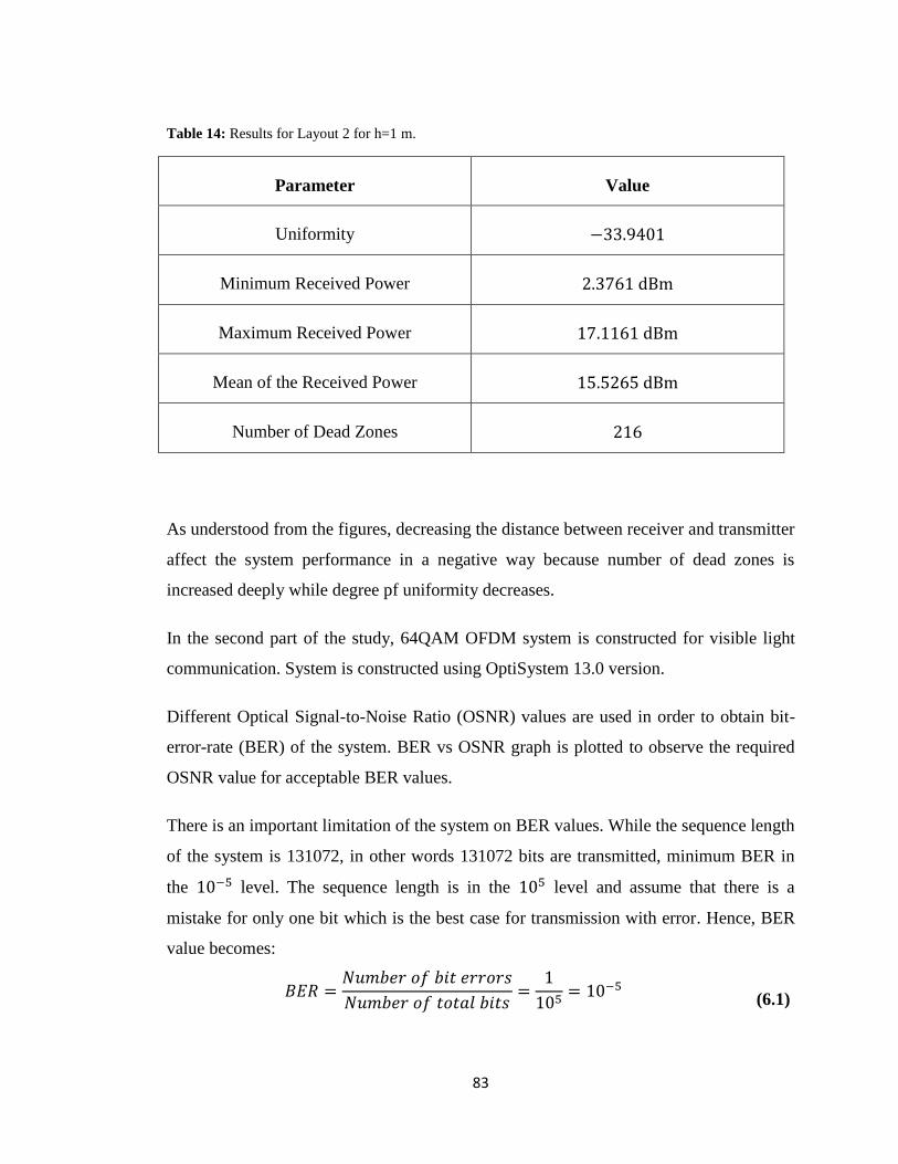
83

Table 14: Results for Layout 2 for h=1 m.

Parameter Value

Uniformity

Minimum Received Power

Maximum Received Power

Mean of the Received Power

Number of Dead Zones

As understood from the figures, decreasing the distance between receiver and transmitter

affect the system performance in a negative way because number of dead zones is

increased deeply while degree pf uniformity decreases.

In the second part of the study, 64QAM OFDM system is constructed for visible light

communication. System is constructed using OptiSystem 13.0 version.

Different Optical Signal-to-Noise Ratio (OSNR) values are used in order to obtain bit-

error-rate (BER) of the system. BER vs OSNR graph is plotted to observe the required

OSNR value for acceptable BER values.

There is an important limitation of the system on BER values. While the sequence length

of the system is 131072, in other words 131072 bits are transmitted, minimum BER in

the level. The sequence length is in the level and assume that there is a

mistake for only one bit which is the best case for transmission with error. Hence, BER

value becomes:

(6.1)

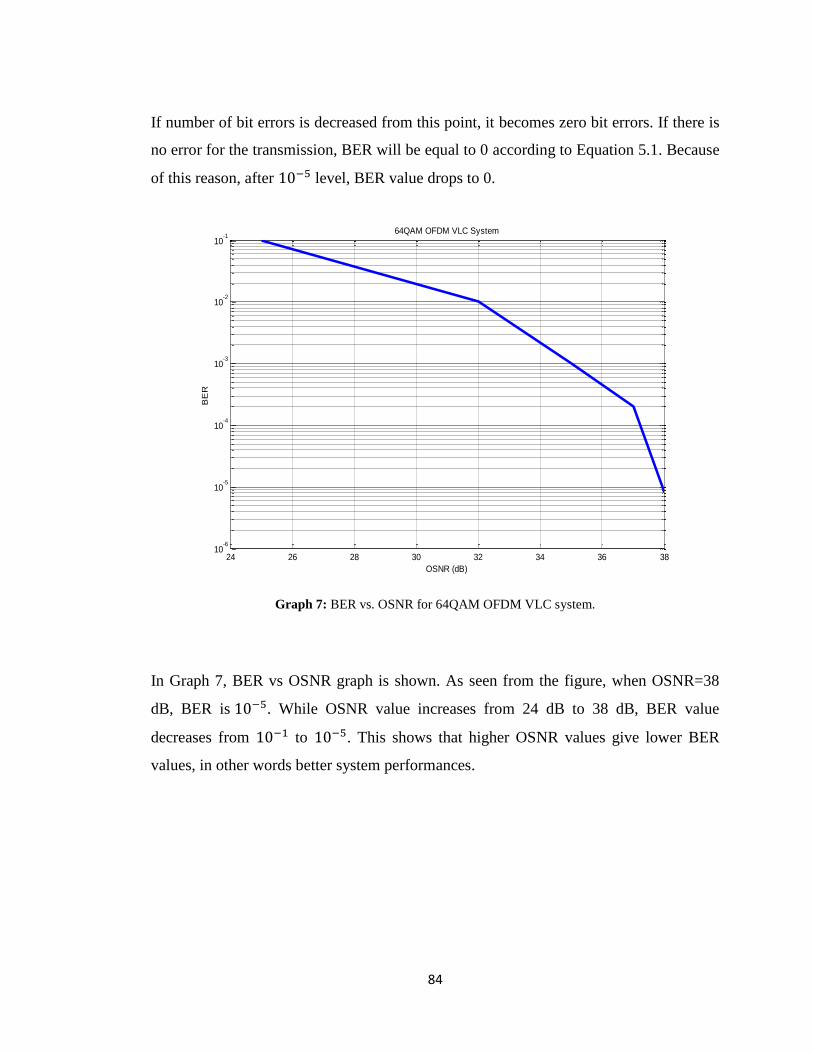
84

If number of bit errors is decreased from this point, it becomes zero bit errors. If there is

no error for the transmission, BER will be equal to 0 according to Equation 5.1. Because

of this reason, after level, BER value drops to 0.

Graph 7: BER vs. OSNR for 64QAM OFDM VLC system.

In Graph 7, BER vs OSNR graph is shown. As seen from the figure, when OSNR=38

dB, BER is . While OSNR value increases from 24 dB to 38 dB, BER value

decreases from to . This shows that higher OSNR values give lower BER

values, in other words better system performances.

24 26 28 30 32 34 36 3810

-6

10-5

10-4

10-3

10-2

10-1

OSNR (dB)

BE

R

64QAM OFDM VLC System

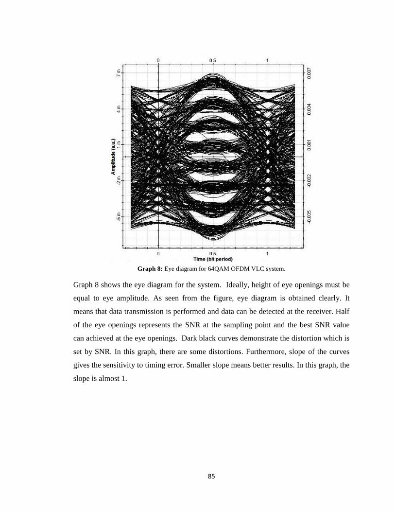
85

Graph 8: Eye diagram for 64QAM OFDM VLC system.

Graph 8 shows the eye diagram for the system. Ideally, height of eye openings must be

equal to eye amplitude. As seen from the figure, eye diagram is obtained clearly. It

means that data transmission is performed and data can be detected at the receiver. Half

of the eye openings represents the SNR at the sampling point and the best SNR value

can achieved at the eye openings. Dark black curves demonstrate the distortion which is

set by SNR. In this graph, there are some distortions. Furthermore, slope of the curves

gives the sensitivity to timing error. Smaller slope means better results. In this graph, the

slope is almost 1.

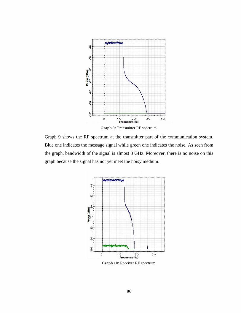
86

Graph 9: Transmitter RF spectrum.

Graph 9 shows the RF spectrum at the transmitter part of the communication system.

Blue one indicates the message signal while green one indicates the noise. As seen from

the graph, bandwidth of the signal is almost 3 GHz. Moreover, there is no noise on this

graph because the signal has not yet meet the noisy medium.

Graph 10: Receiver RF spectrum.

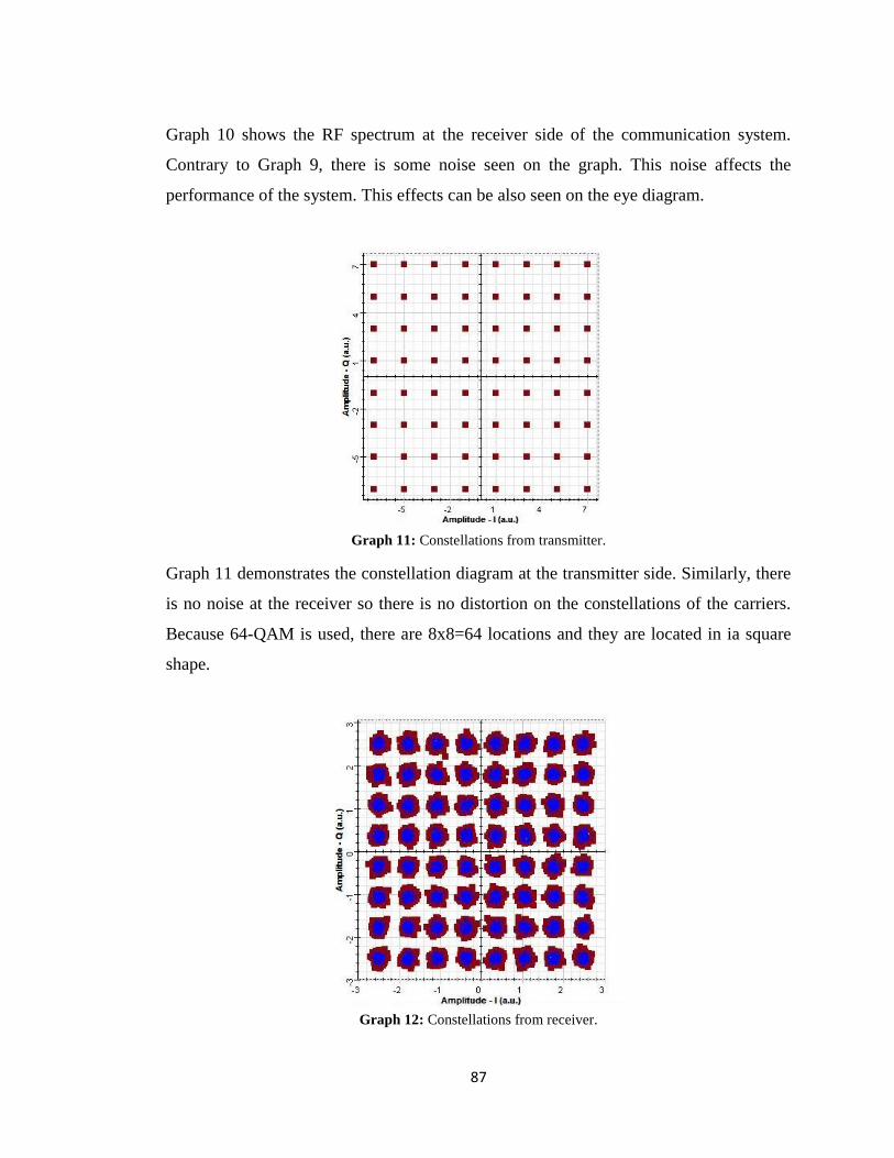
87

Graph 10 shows the RF spectrum at the receiver side of the communication system.

Contrary to Graph 9, there is some noise seen on the graph. This noise affects the

performance of the system. This effects can be also seen on the eye diagram.

Graph 11: Constellations from transmitter.

Graph 11 demonstrates the constellation diagram at the transmitter side. Similarly, there

is no noise at the receiver so there is no distortion on the constellations of the carriers.

Because 64-QAM is used, there are 8x8=64 locations and they are located in ia square

shape.

Graph 12: Constellations from receiver.

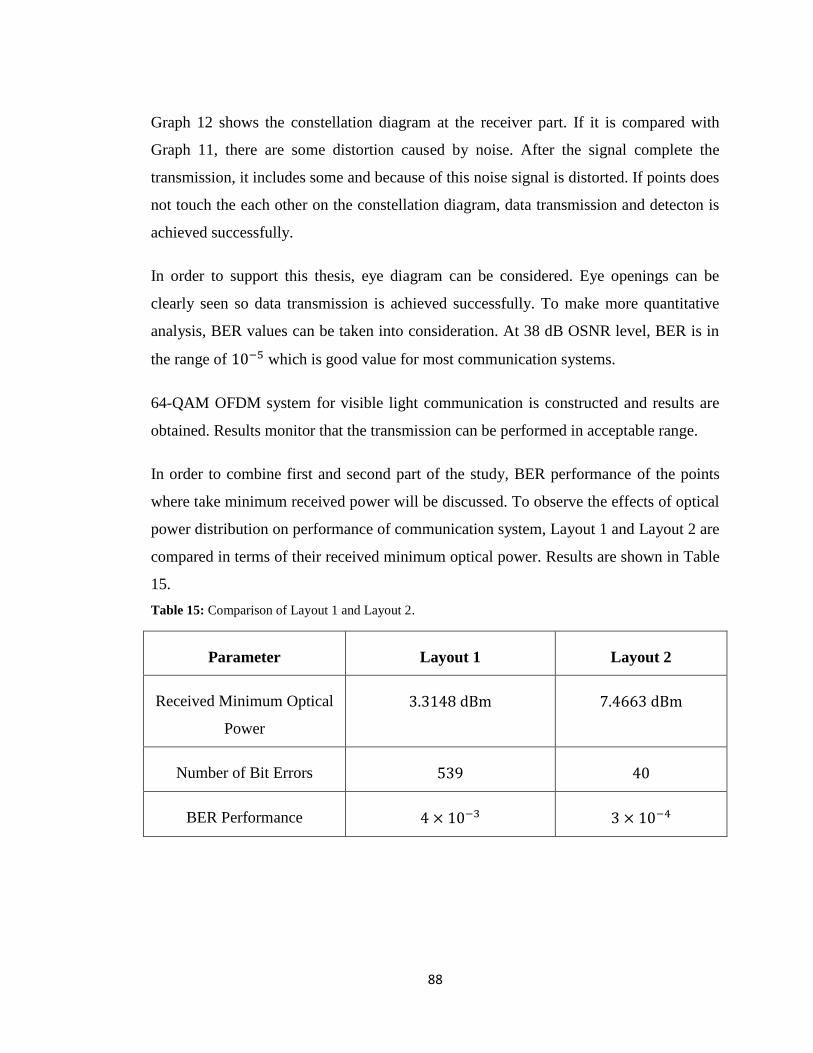
88

Graph 12 shows the constellation diagram at the receiver part. If it is compared with

Graph 11, there are some distortion caused by noise. After the signal complete the

transmission, it includes some and because of this noise signal is distorted. If points does

not touch the each other on the constellation diagram, data transmission and detecton is

achieved successfully.

In order to support this thesis, eye diagram can be considered. Eye openings can be

clearly seen so data transmission is achieved successfully. To make more quantitative

analysis, BER values can be taken into consideration. At 38 dB OSNR level, BER is in

the range of which is good value for most communication systems.

64-QAM OFDM system for visible light communication is constructed and results are

obtained. Results monitor that the transmission can be performed in acceptable range.

In order to combine first and second part of the study, BER performance of the points

where take minimum received power will be discussed. To observe the effects of optical

power distribution on performance of communication system, Layout 1 and Layout 2 are

compared in terms of their received minimum optical power. Results are shown in Table

15.

Table 15: Comparison of Layout 1 and Layout 2.

Parameter Layout 1 Layout 2

Received Minimum Optical

Power

Number of Bit Errors

BER Performance

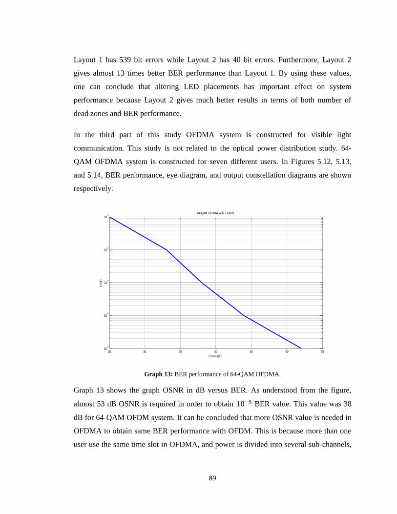
89

Layout 1 has 539 bit errors while Layout 2 has 40 bit errors. Furthermore, Layout 2

gives almost 13 times better BER performance than Layout 1. By using these values,

one can conclude that altering LED placements has important effect on system

performance because Layout 2 gives much better results in terms of both number of

dead zones and BER performance.

In the third part of this study OFDMA system is constructed for visible light

communication. This study is not related to the optical power distribution study. 64-

QAM OFDMA system is constructed for seven different users. In Figures 5.12, 5.13,

and 5.14, BER performance, eye diagram, and output constellation diagrams are shown

respectively.

Graph 13: BER performance of 64-QAM OFDMA.

Graph 13 shows the graph OSNR in dB versus BER. As understood from the figure,

almost 53 dB OSNR is required in order to obtain BER value. This value was 38

dB for 64-QAM OFDM system. It can be concluded that more OSNR value is needed in

OFDMA to obtain same BER performance with OFDM. This is because more than one

user use the same time slot in OFDMA, and power is divided into several sub-channels,

25 30 35 40 45 50 5510

-5

10-4

10-3

10-2

10-1

OSNR (dB)

BE

R

64-QAM OFDMA with 7 Users

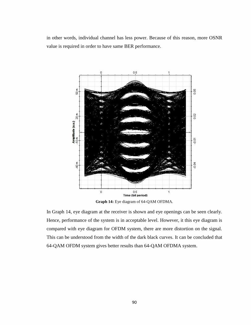
90

in other words, individual channel has less power. Because of this reason, more OSNR

value is required in order to have same BER performance.

Graph 14: Eye diagram of 64-QAM OFDMA.

In Graph 14, eye diagram at the receiver is shown and eye openings can be seen clearly.

Hence, performance of the system is in acceptable level. However, it this eye diagram is

compared with eye diagram for OFDM system, there are more distortion on the signal.

This can be understood from the width of the dark black curves. It can be concluded that

64-QAM OFDM system gives better results than 64-QAM OFDMA system.

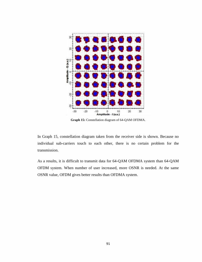
91

Graph 15: Constellation diagram of 64-QAM OFDMA.

In Graph 15, constellation diagram taken from the receiver side is shown. Because no

individual sub-carriers touch to each other, there is no certain problem for the

transmission.

As a results, it is difficult to transmit data for 64-QAM OFDMA system than 64-QAM

OFDM system. When number of user increased, more OSNR is needed. At the same

OSNR value, OFDM gives better results than OFDMA system.

92

CHAPTER SIX

CONCLUSION

Visible light communication is developing area with is superiors. It can solve the health

problems resulted from electromagnetic radiation, it provides much more bandwidth,

and it is securer because visible light cannot pass through walls. With all these

advantages of VLC, it is the main candidate to become an alternative of RF technology.

In this thesis, some fundamental studies belonging to VLC are performed. These studies

are optical power distribution, 64-QAM OFDM system, and 64-QAM OFDMA system,

respectively.

At the optical power distribution study, four different layouts for LED placement on the

ceiling are tested. After simulations of those layouts, it can be concluded that changing

LED placement minimize the number of dead zones. In addition to this, distance

between transmitter and receiver and illumination angle of LED are other important

parameters for the optical power distribution. After this study, dead zones are minimized

and also degree of uniformity is improved importantly.

64-QAM OFDM system is performed and results show that this system is suitable for

visible light communication. Furthermore, 64-QAM OFDMA system is constructed and

similarly it can be used for visible light communication. However, 64-QAM OFDM

system gives better results than 64-QAM OFDMA system.

Finally, BER performance of the layouts are investigated for 64-QAM OFDM system.

Layout which has no dead zone has the best BER performance. From this result, it can

be easily concluded that optical power distribution affects overall system because it has

an effect on BER performance.

93

REFERENCES

[1] Fath, Thilo C. M., “Evaluation of spectrally efficient indoor optical wireless

transmission techniques,” PhD Thesis, The University of Edinburgh, 2013.

[2] Goldsmith, Andrea, “Wireless communications,” Cambridge University Press,

2005. ISBN: 978-0521837163

[3] Z. Ghassemlooy, W. Popoola, and S. Rajbhandari, "Optical Wireless

Communications, System and Channel Modelling with MATLAB," CRC Press,

2013. ISBN: 978-1-4398-5235-4

[4] David L. Andrews (Ed.), "Encylopedia of Applied Spectroscopy," Wiley Press,

2009. ISBN: 978-3-527-40773-6

[5] Tao, Yuyang, et al., "Scheduling for indoor visible light communication based on

graph theory," Optics express 23.3, pp. 2737-2752, 2015. DOI:

10.1364/OE.23.002737

[6] Biagi, Mauro, Tarik Borogovac, and Thomas DC Little, "Adaptive receiver for

indoor visible light communications," Lightwave Technology, Journal of 31.23,

pp. 3676-3686, 2013. ISSN: 0733-8724

[7] H. Elgala, R. Mesleh, H. Haas, and B. Pricope, “OFDM Visible Light Wireless

Communication Based on White LEDs,” 2007 IEEE 65th Vehicle Technology

Conferance - VTC2007-Spring, pp. 2185–2189, 2007.

[8] Bell, Alexander G, “Apparatus for Signaling and Communicating, called

Photophone,” U.S. Patent No. 235,199. 7 Dec. 1880.

[9] R. D. Roberts, “IEEE 802 . 15 . 7 Visible Light Communication : Modulation

Schemes and Dimming Support,” IEEE Communucation Magazine, pp. 72–82,

2012. ISSN: 0163-6804, DOI: 10.1109/MCOM.2012.6163585

[10] Le Minh, Hoa, et al., "100-Mb/s NRZ visible light communications using a

postequalized white LED," Photonics Technology Letters, IEEE 21.15, pp. 1063-

1065, 2009.

[11] Minh, Hoa Le, et al., "High-speed visible light communications using multiple-

resonant equalization," Photonics Technology Letters, IEEE 20.14, pp. 1243-

1245, 2008.

94

[12] Vučić, Jelena, et al., "513 Mbit/s visible light communications link based on DMT-

modulation of a white LED," Journal of lightwave technology, pp. 3512-3518,

2010.

[13] Lee, Kwonhyung, Hyuncheol Park, and John R. Barry, "Indoor channel

characteristics for visible light communications," Communications Letters, IEEE

15.2, pp. 217-219, 2011.

[14] Azhar, Ahmad Helmi, Thomas Tran, and Dominic O'Brien, "A Gigabit/s indoor

wireless transmission using MIMO-OFDM visible-light communications,"

Photonics Technology Letters, IEEE 25.2, pp. 171-174, 2013.

[15] Minh, Hoa Le, et al., "80 Mbit/s visible light communications using pre-equalized

white LED," Optical Communication, ECOC 2008. 34th European Conference

on. IEEE, 2008.

[16] Li, Honglei, et al., "High bandwidth visible light communications based on a post-

equalization circuit," Photonics Technology Letters, IEEE 26.2, pp. 119-122,

2014.

[17] Zhou, Zhou, Mohsen Kavehrad, and Peng Deng, "Indoor positioning algorithm

using light-emitting diode visible light communications," Optical Engineering

51.8, 2012.

[18] Zhang, Shuailong, et al., "1.5 Gbit/s multi-channel visible light communications

using CMOS-controlled GaN-based LEDs," Journal of Lightwave Technology,

2013.

[19] Wang, Yuanquan, et al., "Demonstration of 575-Mb/s downlink and 225-Mb/s

uplink bi-directional SCM-WDM visible light communication using RGB LED

and phosphor based LED," Optics express 21.1, 2013.

[20] H. J. R. Dutton, “Understanding Optical Communications,” New Jersey: Prentice

Hall PTR, 1998. ISBN: 007-6092003847

[21] Morkoç, Hadis, "Handbook of Nitride Semiconductors and Devices, Materials

Properties, Physics and Growth," Vol. 3. John Wiley & Sons, 2009. ISBN: 978-

3-527-40839-9

[22] Coldren, Larry A., Scott W. Corzine, and Milan L. Mashanovitch. "Diode lasers

and photonic integrated circuits," Vol. 218. John Wiley & Sons, 2012. ISBN:

978-0470484128

95

[23] Zheludev, Nikolay. "The life and times of the LED-a 100-year history," Nature

Photonics 1.4, pp. 189-192, 2007. ISSN: 1749-4885, DOI:

10.1038/nphoton.2007.34

[24] Baev, V. M., T. Latz, and P. E. Toschek. "Laser intracavity absorption

spectroscopy," Applied Physics B 69.3, pp. 171-202, 1999. ISSN: 0021-8979,

DOI: 10.1007/s003400050793

[25] Agrawal, Goving P., "Fiber-Optic Communications Systems," (3rd ed.), vol. 6.

John Wiley, New York, 2002. ISBN: 978-0470505113

[26] Agrawal, Goving P. and Dutta, N.K., “Semiconductor Lasers,", (2nd

ed.), VNR,

New York, 1993. ISBN: 0-442-01102-4

[27] Liu, Zhixin, et al., "Modulator-free quadrature amplitude modulation signal

synthesis," Nature communications 5, 2014. ISSN: 2041-1723

[28] Sharpe, Lindsay T.,Stockman, A., Jagla, W. and Jägle, H., "A luminous efficiency

function, V*(λ), for daylight adaptation." Journal of Vision 5.11, 2005. ISSN:

1534-7362, DOI: 10.1167/5.11.3

[29] Komine, T. and Nakagawa, M., “Fundamental analysis for visible-light

communication system using LED lights,” IEEE Trans. Consum. Electron., vol.

50, no. 1, pp. 100–107, 2004. ISSN: 0098-3063, DOI:

10.1109/TCE.2004.1277847

[30] Haykin, Simon, “Communication systems.” John Wiley & Sons, 2008. ISBN:

978-9971513054

[31] Saleh, Bahaa EA, Malvin Carl Teich, and Bahaa E. Saleh., "Fundamentals of

Photonics," Vol. 22. New York: Wiley, 1991. ISBN: 978-0471358329

[32] Gooch & Housego, "IRX Series CdTe Pockels Cell," Datasheet.

[33] Peucheret, Christophe, "Direct and External Modulation of Light," Lecture Notes,

Technical University of Denmark, Denmark, 2009.

[34] Piprek, J., et al. "High-efficiency MQW Electroabsorption Modulators," ECS

Proc. International Symposium on Integrated Optoelectronics, Philadelphia, USA,

2002.

[35] Gordon, E. I., and J. D. Rigden. "The Fabry‐Perot Electrooptic Modulator." Bell

System Technical Journal 42.1, pp. 155-179, 1963.

96

[36] Agilent Application Note, "1298. Digital modulation in communications systems-

An introduction," Hewlett-Packard Company, 1997

[37] Jawla, Shashi, and R. K. Singh, "Different Modulation Formats Used In Optical

Communication System," IOSR Journal of Electronics and Communication

Engineering (IOSR-JECE) 8.4, 2013.ISSN: 2278-8735

[38] Thomas, C., Martin Weidner, and S. H. Durrani, "Digital amplitude-phase keying

with M-ary alphabets," Communications, IEEE Transactions on 22.2, pp. 168-

180, 1974. ISSN: 0090-6778, DOI: 10.1109/TCOM.1974.1092165

[39] Peebles Jr, Peyton Z., "Digital communication systems," Englewood Cliffs, NJ,

Prentice-Hall, Inc., 1987. ISBN: 978-0132119702

[40] Simon, Marvin K. "Single integral representations of certain integer powers of the

Gaussian Q-function and their application," Communications Letters, IEEE 6.12,

pp. 532-534, 2002. ISSN: 1089-7798

[41] Bennett, William Ralph. "Spectra of quantized signals." Bell System Technical

Journal 27.3, pp. 446-472, 1948.

[42] Rogers, John WM, and Calvin Plett, "Radio frequency integrated circuit design,"

Artech House, 2010. ISBN: 978-1580535021

[43] Proakis, John G., Salehi, M., "Digital communications," (4th

ed.), McGraw-Hill,

New York, 1995.

[44] Cho, Yong Soo, Kim, J., Yang, W. Y. and Kang, C.G., "MIMO-OFDM wireless

communications with MATLAB," John Wiley & Sons, 2010. ISBN: 978-

0470825617

[45] Osgood, B., “The Fourier Transform and its Applications - Lecture Notes,”

Electrical Engineering Department, Stanford University, 2010.

[46] Tsonev, Dobroslav, Sinan Sinanovic, and Harald Haas., "Enhanced subcarrier

index modulation (SIM) OFDM," IEEE GLOBECOM Workshops (GC Wkshps),

2011.

[47] Armstrong, Jean, "OFDM for optical communications," Lightwave Technology,

Journal of 27.3, pp. 189-204, 2009. ISSN: 0733-8724

[48] Tarokh, Vahid, "New directions in wireless communications research," Springer,

2009. ISBN: 978-1441906724

97

[49] Prasad, Ramjee, "OFDM for wireless communications systems," Artech House,

2004. ISBN: 978-1580537964

[50] Shannon, Claude Elwood, "A mathematical theory of communication," ACM

SIGMOBILE Mobile Computing and Communications Review 5.1, pp. 3-55,

2001. ISSN: 1559-1662

[51] Lecture Notes, “Lecture 8 - Convolutional Coding,” Massachusetts Instute of

Technology (MIT), October 2010.

[52] Clarke, C. K. P., "Reed-Solomon error correction," British Broadcasting

Corporation R&D White Paper, WHP 31, 2002.

[53] Shannon, Claude E., "Communication in the presence of noise," Proceedings of

the IRE 37.1, pp. 10-21, 1949.

[54] Prasad, Ramjee, and Fernando J. Velez, "WiMAX networks: techno-economic

vision and challenges," Springer Science & Business Media, 2010. ISBN: 978-

9048187515

[55] M. P. Michele Morelli, Jay Kuo, “Synchronization Techniques for Orthogonal

Frequency Division Multiple Access (OFDMA): A Tutorial Review,” Proc. IEEE,

vol. 95, no. 7, pp. 1394 – 1427, 2007. ISSN: 0018-9219, DOI:

10.1109/JPROC.2007.897979

[56] Prasad, S. S., C. K. Shukla, and Raad Farhood Chisab, "Performance Analysis of

OFDMA in LTE," Computing Communication & Networking Technologies

(ICCCNT), 2012 Third International Conference on, IEEE, 2012.