Optic-Flow Based Control of a 46g Quadrotor

Adrien Briod1, Jean-Christophe Zufferey2 and Dario Floreano1

Abstract— We aim at developing autonomous miniature hov-ering flying robots capable of navigating in unstructured GPS-denied environments. A major challenge is the miniaturiza-tion of the embedded sensors and processors allowing suchplatforms to fly autonomously. In this paper, we propose anovel ego-motion estimation algorithm for hovering robotsequipped with inertial and optic-flow sensors that runs in real-time on a microcontroller. Unlike many vision-based methods,this algorithm does not rely on feature tracking, structureestimation, additional distance sensors or assumptions aboutthe environment. Key to this method is the introduction ofthe translational optic-flow direction constraint (TOFDC), whichdoes not use the optic-flow scale, but only its direction tocorrect for inertial sensor drift during changes of direction.This solution requires comparatively much simpler electronicsand sensors and works in environments of any geometries.We demonstrate the implementation of this algorithm on aminiature 46g quadrotor for closed-loop position control.

I. INTRODUCTION

Using robots instead of risking human lives for explorationmissions in dangerous environments has great safety andefficiency benefits. Flying robots have many advantages asthey provide an elevated view-point and can navigate aboverubble more efficiently than ground-based robots. However,most flying platforms are unstable by design and needto be controlled in closed-loop in order to achieve usefultasks, such as remaining in a stable position in the air orfollowing trajectories. In order to solve this challenge inGPS-denied environments, embedded sensors have to be usedfor position or velocity estimation, which is called ego-motion estimation. Payload being limited on flying platforms,it is of great interest to miniaturize the hardware required forego-motion estimation so as to reduce the size of autonomousMicro Aerial Vehicles (MAV).

Because of their versatility and relatively low weight,monocular vision sensors are often used for ego-motionestimation. Monocular vision sensors are affected by thescale ambiguity, in other words the inability to distinguishthe scale of a translation [1]. Visual information is usuallyconverted to metric measurements thanks to the so-called’scale factor’, which is often identified thanks to additionalsensors. One of the most successful solution is inertial SLAM(Simultaneous Localization and Mapping) [2], [3], [4], [5],[6]. In this case, the scale factor is eventually obtained thanksto accelerometers and is observable if linear accelerations are

Authors are with: (1) the Laboratory of Intelligent Systems (LIS)http://lis.epfl.ch, Ecole Polytechnique Federale de Lausanne(EPFL), 1015 Lausanne, Switzerland, (2) SenseFly Ltd, 1024 Ecublens,Switzerland

This research was supported by the Swiss National Science Foundationthrough the National Centre of Competence in Research (NCCR) Robotics.

Contact e-mail: adrien.briod@epfl.ch.

Fig. 1. A 46g quadrotor capable of autonomous flight thanks to inertialsensors and five 0.8g optic-flow sensors, each providing a 2D optic-flowmeasurement, and arranged in order to cover a wide field-of-view (dashedlines are the viewing directions).

present [7]. These methods allow for absolute positioning andeven reconstruct the 3D structure of the environment in theprocess.

SLAM algorithms require relatively high processing powerand memory, which may result in fairly bulky setups. Asimpler approach consists of fusing inertial data directly withthe epipolar constraint [8], [9], [10], [11]. Applying directlythis constraint bypasses the need for structure re-constructionand thus reduces significantly the amount of processing andmemory required [9], while it can still take advantage oferror corrections from features tracked multiple frames apart[8], [10]. However, the scale of the motion is not providedby epipolar constraint updates, and the relative scale is notconserved, which provokes generally large estimation errorsas mentioned in [9]. An interesting approach in [11] suggeststo estimate the average depth of the tracked features, so thatthe camera can be used as a metric sensor.

However, methods based on feature tracking remain rel-atively complex because they require cameras with goodenough resolution and sufficient computing power for thefeature extraction and matching algorithms [12]. On the otherhand, comparatively very simple methods and sensors existfor optic-flow extraction. Optic-flow is the apparent motionof the scene at discrete points in the field-of-view, and cantypically be obtained from the variation of pixel intensityover time [13], [14]. Optic-flow sensors work at low resolu-tion and thus exist in very small and cheap packages [15],[16]. Also, optic-flow can be extracted from a scene that doesnot present recognizable features, such as blurry textures or

repetitive patterns, or even in the dark [15]. Optic-flow hasbeen used on MAVs in the past for bio-inspired obstacleavoidance [17], [18], or speed regulation [19], [20].

Optic-flow has two main drawbacks compared to featuretracking when it comes to ego-motion estimation: a) Optic-flow information is only related to motion and generated byunidentified visual cues, which prevents it to be used forabsolute localization like feature tracking-based algorithms.Ego-motion obtained from optic-flow is thus very likely topresent position drift (error accumulation over time), becauseit is obtained by integrating velocity estimates. b) The scalefactor affecting optic-flow measurements changes at eachstep because the visual cues generating optic-flow are alwaysdifferent. On the other hand, feature tracking typically allowsto retain a constant relative scale between all measurements.It is thus comparatively harder to convert optic-flow infor-mation into a metric value. For these reasons, optic-flowis generally considered not suitable for visual odometryapplications [1].

It is however possible to estimate the direction of motionfrom optic-flow measurements [21] and even a velocity thatis scaled inversely proportionally to the average depth ofthe environment, which is used in [20] to control a MAVhovering at a fixed point. However it is unclear how thisstrategy can handle maneuvers provoking the depth to changeconstantly. Inertial sensors are used in [22] and [23] to obtainthe scale of optic-flow measurements, but the methods onlywork over flat surfaces. A successful method that allows tosolve the scale ambiguity problem is to couple optic-flowsensors with distance sensors, which continuously providethe absolute scale. For example in [24] or [25], an ultrasonicdistance sensor is used together with a camera pointingdownwards, which results in a very good velocity estimationand thus low position drift. However, such a solution addsbulkiness to the system and only works below the limitedrange of the distance sensor.

It can be seen from the prior art that most solutions usevision as a metric sensor for ego-motion measurement, whichrequires to determine the scale of the visual information. Fea-ture tracking keeps the scale factor constant, which facilitatesits estimation because it has to be obtained once and for all[6] (possibly with small adjustments over time). On the otherhand, optic-flow offers better potential for miniaturization,but is hard to convert into metric information, especially inunstructured environments where no simplifying assumptionscan be made.

In this paper, we present a novel algorithm for ego-motionestimation based on optic-flow and inertial sensors whereit is not attempted to convert optic-flow information into ametric measurement. We then demonstrate its viability andminiaturization potential by using it for closed-loop controlof a miniature hovering robot. Section II describes an EKFimplementation of the algorithm, section III presents a 46gquadrotor equipped with 5 optic-flow sensors and able ofrunning the algorithm in real time on a microcontroller.Finally, section IV describes briefly the results obtainedduring autonomous flights in different environments.

a)

b)

c)trajectoryrobotvelocityuncertainty

y

x

z

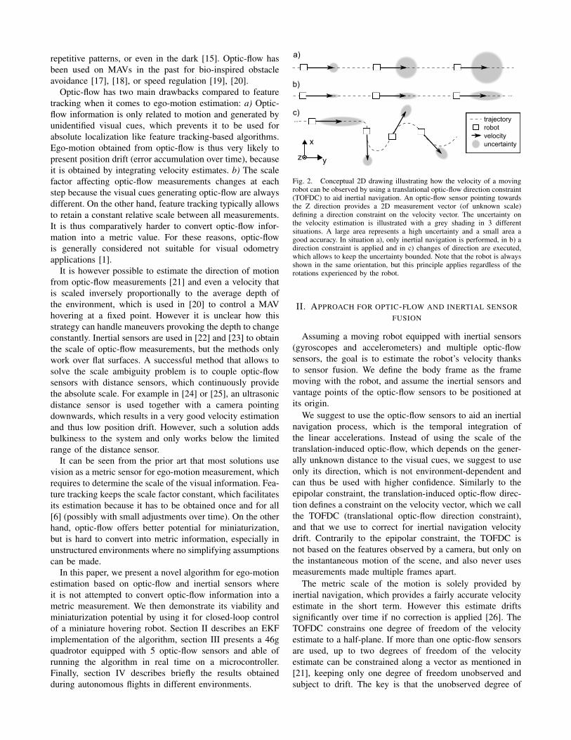
Fig. 2. Conceptual 2D drawing illustrating how the velocity of a movingrobot can be observed by using a translational optic-flow direction constraint(TOFDC) to aid inertial navigation. An optic-flow sensor pointing towardsthe Z direction provides a 2D measurement vector (of unknown scale)defining a direction constraint on the velocity vector. The uncertainty onthe velocity estimation is illustrated with a grey shading in 3 differentsituations. A large area represents a high uncertainty and a small area agood accuracy. In situation a), only inertial navigation is performed, in b) adirection constraint is applied and in c) changes of direction are executed,which allows to keep the uncertainty bounded. Note that the robot is alwaysshown in the same orientation, but this principle applies regardless of therotations experienced by the robot.

II. APPROACH FOR OPTIC-FLOW AND INERTIAL SENSORFUSION

Assuming a moving robot equipped with inertial sensors(gyroscopes and accelerometers) and multiple optic-flowsensors, the goal is to estimate the robot’s velocity thanksto sensor fusion. We define the body frame as the framemoving with the robot, and assume the inertial sensors andvantage points of the optic-flow sensors to be positioned atits origin.

We suggest to use the optic-flow sensors to aid an inertialnavigation process, which is the temporal integration ofthe linear accelerations. Instead of using the scale of thetranslation-induced optic-flow, which depends on the gener-ally unknown distance to the visual cues, we suggest to useonly its direction, which is not environment-dependent andcan thus be used with higher confidence. Similarly to theepipolar constraint, the translation-induced optic-flow direc-tion defines a constraint on the velocity vector, which we callthe TOFDC (translational optic-flow direction constraint),and that we use to correct for inertial navigation velocitydrift. Contrarily to the epipolar constraint, the TOFDC isnot based on the features observed by a camera, but only onthe instantaneous motion of the scene, and also never usesmeasurements made multiple frames apart.

The metric scale of the motion is solely provided byinertial navigation, which provides a fairly accurate velocityestimate in the short term. However this estimate driftssignificantly over time if no correction is applied [26]. TheTOFDC constrains one degree of freedom of the velocityestimate to a half-plane. If more than one optic-flow sensorsare used, up to two degrees of freedom of the velocityestimate can be constrained along a vector as mentioned in[21], keeping only one degree of freedom unobserved andsubject to drift. The key is that the unobserved degree of

de-rotation TOFDC

Viewing direction

calibration

N optic-flow sensors

Rate gyroscopes

Accelerometers

Attitude estimation

Gravity

compensation

normalization

Centrifugal acc.

compensation Acceleration

integration

Velocity,

Acc. biases

Odometry

a u

p pt pt

Rs

ω

ωcalib , v R

a

ωcalib

R

velocity

Extended Kalman Filter

position

v

100Hz

25Hz

r

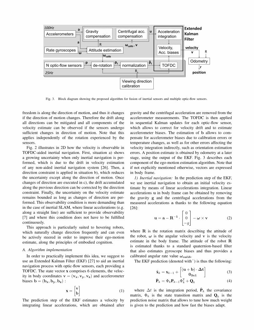
Fig. 3. Block diagram showing the proposed algorithm for fusion of inertial sensors and multiple optic-flow sensors.

freedom is along the direction of motion, and thus it changesif the direction of motion changes. Therefore the drift alongall directions can be mitigated and all components of thevelocity estimate can be observed if the sensors undergosufficient changes in direction of motion. Note that thisapplies independently of the rotation experienced by thesensors.

Fig. 2 illustrates in 2D how the velocity is observable inTOFDC-aided inertial navigation. First, situation a) showsa growing uncertainty when only inertial navigation is per-formed, which is due to the drift in velocity estimationof any non-aided inertial navigation system [26]. Then, adirection constraint is applied in situation b), which reducesthe uncertainty except along the direction of motion. Oncechanges of direction are executed in c), the drift accumulatedalong the previous direction can be corrected by the directionconstraint. Finally, the uncertainty on the velocity estimateremains bounded as long as changes of direction are per-formed. This observability condition is more demanding thanin the case of inertial SLAM, where linear accelerations (e.g.along a straight line) are sufficient to provide observability[7] and where this condition does not have to be fulfilledcontinuously.

This approach is particularly suited to hovering robots,which naturally change direction frequently and can evenbe actively steered in order to improve their ego-motionestimate, along the principles of embodied cognition.

A. Algorithm implementation

In order to practically implement this idea, we suggest touse an Extended Kalman Filter (EKF) [27] to aid an inertialnavigation process with optic-flow sensors, each providing aTOFDC. The state vector x comprises 6 elements, the veloc-ity in body coordinates v = (vx,vy,vz) and accelerometerbiases b = (bx,by,bz) :

x =

[vb

](1)

The prediction step of the EKF estimates a velocity byintegrating linear accelerations, which are obtained after

gravity and the centrifugal acceleration are removed from theaccelerometer measurements. The TOFDC is then appliedin sequential Kalman updates for each optic-flow sensor,which allows to correct for velocity drift and to estimateaccelerometer biases. The estimation of b allows to com-pensate for accelerometer biases due to calibration errors ortemperature changes, as well as for other errors affecting thevelocity integration indirectly, such as orientation estimationerrors. A position estimate is obtained by odometry at a laterstage, using the output of the EKF. Fig. 3 describes eachcomponent of the ego-motion estimation algorithm. Note thatif not explicitly mentioned otherwise, vectors are expressedin body frame.

1) Inertial navigation: In the prediction step of the EKF,we use inertial navigation to obtain an initial velocity es-timate by means of linear accelerations integration. Linearaccelerations u in body frame can be obtained by removingthe gravity g and the centrifugal accelerations from themeasured accelerations a thanks to the following equation[26]:

u = a−R−1 ·

00−g

− ω × v (2)

where R is the rotation matrix describing the attitude ofthe robot, ω is the angular velocity and v is the velocityestimate in the body frame. The attitude of the robot Ris estimated thanks to a standard quaternion-based filterthat also estimates gyroscope biases and thus provides acalibrated angular rate value ωcalib.

The EKF prediction (denoted with˜) is thus the following:

xk = xk−1 +

[(u + b) ·∆t

03x1

](3)

Pk = ΦkPk−1ΦTk + Qk (4)

where ∆t is the integration period, Pk the covariancematrix, Φk is the state transition matrix and Qk is theprediction noise matrix that allows to tune how much weightis given to the prediction and how fast the biases adapt.

px

Zs

XsYs

py d

vv

I

I

pt

Fig. 4. The direction of the translational optic-flow vector pt depends onthe velocity v and the unit vector d, pointing toward the viewing directionof the sensor. The translational optic-flow direction constraint (TOFDC)is expressed in the image plane I , and states that the projection vI ofthe velocity vector v onto the image plane I has to be collinear to thetranslational optic-flow vector pt and of opposite direction.

2) Optic-flow correction: Assuming a projection of thescene on a unit sphere centered at the vantage point, eachoptic-flow measurement can be expressed as a 3D vectortangent to the unit sphere and perpendicular to the viewingdirection [28]:

p = − ω × d︸ ︷︷ ︸pr

−v − (v · d)d

D︸ ︷︷ ︸pt

(5)

where d is a unit vector describing the viewing direction,ω the angular speed vector, v the translational velocityvector and D the distance to the object seen by the sensor.The measured optic-flow p can be expressed in two parts,namely the rotation-induced or ’rotational’ optic-flow pr andtranlsation-induced or ’translational’ optic-flow pt.

Only the translational optic-flow pt is useful for velocityestimation, and the rotational optic-flow pr is consideredhere as a disturbance that is removed from the measurementp thanks to a process called de-rotation [29]. We use amethod that we proposed in [30] able to automaticallycalibrate the viewing direction of optic-flow sensors andexecute the de-rotation thanks to rate gyroscopes. In theory,rotations should thus not affect the outcome of the algorithm,but in practice the de-rotation procedure may introduce noise,especially if the amplitude of rotational optic-flow is muchlarger than translational optic-flow.

To express the translational optic-flow direction constraint,we define a sensor frame (Xs, Ys, Zs) whose Zs axis isaligned with the viewing direction and whose Xs and Ys axesdefine the image plane of the optic-flow sensor, as shown inFig. 4. We can thus express the following vectors:

pt,s =

pt,xpt,y0

, ds =

001

and vs = Rsvr =

vs,xvs,yvs,z

(6)

Where vs is the velocity vector expressed in the sensor

frame and Rs is the rotation matrix that describes theorientation of the sensor with respect to the body frame.

The translational optic-flow can be rewritten as:pt,xpt,y0

= − 1

D

vs,xvs,y0

(7)

which is a relation between 2D vectors:

vI = −D · pt,I (8)

where pt,I = [pt,x , pt,y ] is the 2D translational optic-flowmeasurement and

vI =

[vs,xvs,y

]=

[rs,11 rs,12 rs,13rs,21 rs,22 rs,23

]v (9)

is the projection of the velocity on the image plane. rs,ij arethe elements of the first two rows of the rotation matrix Rs,which are obtained thanks to an initial calibration process,for instance as described in [30].

Equation (8) highlights the difficulty to convert optic-flow to a metric velocity measurement, because the distanceD is apriori unknown and changes constantly in clutteredenvironments. However equation (8) states that, regardlessof D, the projection vI of the velocity vector v onto theimage plane I has to be collinear to the translational optic-flow vector pt,I and of opposite direction. This constraint iswhat we call the translational optic-flow direction constraint(TOFDC), which can be expressed by using normalizedvectors :

pt,I = −vI (10)

where pt,I and vI are unit vectors:

pt,I =pt,I

||pt,I ||and vI =

vI

||vI ||(11)

Considering the following Kalman update equations:

Kk = PkHTk(HkPkHT

k + Rk)−1 (12)xk = xk + Kk(zk − h[xk]) (13)

Pk = (I −KkHk)Pk (14)

we suggest to use the following measurement sequentiallyfor each optic-flow sensor:

zk = pt,I (15)

and the following non-linear measurement model:

h[xk] = −vI (16)

The corresponding jacobian matrix is obtained from Hk =∂h[x]∂x . The 2 × 2 measurement noise matrix is set to Rk =diag(σ2

of ) where σof describes the noise on the optic-flowmeasurement and can typically be varied in function of someknown quality indicators (such as amount of rotations, oroptic-flow norm).

3) Odometry: As a last step, the velocity obtained in bodyframe v needs to be converted in earth frame and integratedover time to obtain a position estimate r:

rk = rk−1 + R−1 · v ·∆t (17)

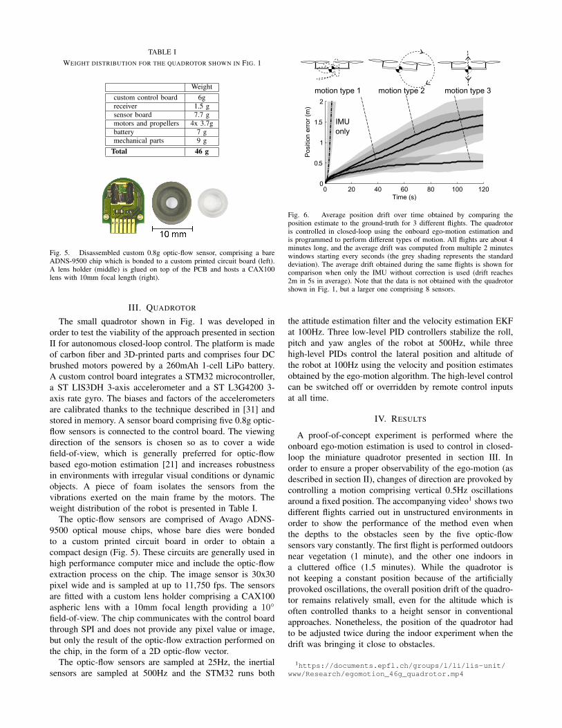
TABLE IWEIGHT DISTRIBUTION FOR THE QUADROTOR SHOWN IN FIG. 1

Weightcustom control board 6greceiver 1.5 gsensor board 7.7 gmotors and propellers 4x 3.7gbattery 7 gmechanical parts 9 g

Total 46 g

Fig. 5. Disassembled custom 0.8g optic-flow sensor, comprising a bareADNS-9500 chip which is bonded to a custom printed circuit board (left).A lens holder (middle) is glued on top of the PCB and hosts a CAX100lens with 10mm focal length (right).

III. QUADROTOR

The small quadrotor shown in Fig. 1 was developed inorder to test the viability of the approach presented in sectionII for autonomous closed-loop control. The platform is madeof carbon fiber and 3D-printed parts and comprises four DCbrushed motors powered by a 260mAh 1-cell LiPo battery.A custom control board integrates a STM32 microcontroller,a ST LIS3DH 3-axis accelerometer and a ST L3G4200 3-axis rate gyro. The biases and factors of the accelerometersare calibrated thanks to the technique described in [31] andstored in memory. A sensor board comprising five 0.8g optic-flow sensors is connected to the control board. The viewingdirection of the sensors is chosen so as to cover a widefield-of-view, which is generally preferred for optic-flowbased ego-motion estimation [21] and increases robustnessin environments with irregular visual conditions or dynamicobjects. A piece of foam isolates the sensors from thevibrations exerted on the main frame by the motors. Theweight distribution of the robot is presented in Table I.

The optic-flow sensors are comprised of Avago ADNS-9500 optical mouse chips, whose bare dies were bondedto a custom printed circuit board in order to obtain acompact design (Fig. 5). These circuits are generally used inhigh performance computer mice and include the optic-flowextraction process on the chip. The image sensor is 30x30pixel wide and is sampled at up to 11,750 fps. The sensorsare fitted with a custom lens holder comprising a CAX100aspheric lens with a 10mm focal length providing a 10◦

field-of-view. The chip communicates with the control boardthrough SPI and does not provide any pixel value or image,but only the result of the optic-flow extraction performed onthe chip, in the form of a 2D optic-flow vector.

The optic-flow sensors are sampled at 25Hz, the inertialsensors are sampled at 500Hz and the STM32 runs both

0 20 40 60 80 100 1200

0.5

1

1.5

2

Time (s)

Pos

ition

err

or (

m)

motion type 1 motion type 2 motion type 3

IMU only

Fig. 6. Average position drift over time obtained by comparing theposition estimate to the ground-truth for 3 different flights. The quadrotoris controlled in closed-loop using the onboard ego-motion estimation andis programmed to perform different types of motion. All flights are about 4minutes long, and the average drift was computed from multiple 2 minuteswindows starting every seconds (the grey shading represents the standarddeviation). The average drift obtained during the same flights is shown forcomparison when only the IMU without correction is used (drift reaches2m in 5s in average). Note that the data is not obtained with the quadrotorshown in Fig. 1, but a larger one comprising 8 sensors.

the attitude estimation filter and the velocity estimation EKFat 100Hz. Three low-level PID controllers stabilize the roll,pitch and yaw angles of the robot at 500Hz, while threehigh-level PIDs control the lateral position and altitude ofthe robot at 100Hz using the velocity and position estimatesobtained by the ego-motion algorithm. The high-level controlcan be switched off or overridden by remote control inputsat all time.

IV. RESULTS

A proof-of-concept experiment is performed where theonboard ego-motion estimation is used to control in closed-loop the miniature quadrotor presented in section III. Inorder to ensure a proper observability of the ego-motion (asdescribed in section II), changes of direction are provoked bycontrolling a motion comprising vertical 0.5Hz oscillationsaround a fixed position. The accompanying video1 shows twodifferent flights carried out in unstructured environments inorder to show the performance of the method even whenthe depths to the obstacles seen by the five optic-flowsensors vary constantly. The first flight is performed outdoorsnear vegetation (1 minute), and the other one indoors ina cluttered office (1.5 minutes). While the quadrotor isnot keeping a constant position because of the artificiallyprovoked oscillations, the overall position drift of the quadro-tor remains relatively small, even for the altitude which isoften controlled thanks to a height sensor in conventionalapproaches. Nonetheless, the position of the quadrotor hadto be adjusted twice during the indoor experiment when thedrift was bringing it close to obstacles.

1https://documents.epfl.ch/groups/l/li/lis-unit/www/Research/egomotion_46g_quadrotor.mp4

Further experiments will focus on characterizing the per-formance of the method for multiple motion types thanksto a ground truth. For this, a similar but bigger quadrotorequipped with motion capture beacons and 8 optic-flowsensors was built. Preliminary results show that the positiondrift is of 50cm in average after 2 minutes of flight when0.5Hz vertical oscillations are controlled (figure 6). On theother hand, the position drift is higher for other motion types,such as stationary flight or 0.5Hz oscillations along a verticalcircle.

V. CONCLUSION

This paper describes a novel method for ego-motion esti-mation and its implementation on a miniature quadrotor. Byusing the translational optic-flow direction only, this methodworks in environments of any geometry without relying ondepth estimation and without converting visual informationinto a metric measurement.

While the proposed method does not reach the accuracyof techniques based on feature tracking, it shows sufficientprecision for closed-loop control of MAVs. The advantageof our approach is that it can be implemented on simplemicrocontrollers and requires very light-weight sensors, andcan thus be embedded on smaller flying platforms whosesize, agility and robustness are beneficial when exploringtight spaces.

Future work will focus on reactive obstacle avoidance,which can be achieved by using the amplitude of thetranslational optic-flow. The implementation of RANSACfor outlier rejection will be explored in order to betterhandle moving objects. Finally, future miniaturization mayenable an implementation on even smaller flying robots,such as micromechanical flying insects, whose biologicalcounterparts coincidentally also tend to never fly straight.

VI. ACKNOWLEDGMENT

The authors would like to thank the Parc Scientifique officeof Logitech at EPFL for providing the bare mouse chips.The authors also want to thank Przemyslaw Kornatowskifor helping designing and manufacturing the flying platform.Part of this work has been submitted for patenting (Europeanpatent filing number EP12191669.6).

REFERENCES

[1] D. Scaramuzza and F. Fraundorfer, “Visual Odometry [Tutorial],”IEEE Robot. Autom. Mag., vol. 18, no. 4, pp. 80–92, Dec. 2011.

[2] P. Corke, J. Lobo, and J. Dias, “An Introduction to Inertial and VisualSensing,” Int. J. Rob. Res., vol. 26, no. 6, pp. 519–535, Jun. 2007.

[3] J. Kelly and G. S. Sukhatme, “Visual-Inertial Sensor Fusion:Localization, Mapping and Sensor-to-Sensor Self-calibration,” Int. J.Rob. Res., vol. 30, no. 1, pp. 56–79, Nov. 2010.

[4] E. S. Jones and S. Soatto, “Visual-inertial navigation, mapping andlocalization: A scalable real-time causal approach,” Int. J. Rob. Res.,vol. 30, no. 4, pp. 407–430, Jan. 2011.

[5] D. Scaramuzza et al., “Vision-Controlled Micro Flying Robots : fromSystem Design to Autonomous Navigation and Mapping in GPS-denied Environments,” IEEE Robot. Autom. Mag., 2013.

[6] S. Weiss, M. W. Achtelik, M. Chli, and R. Siegwart, “VersatileDistributed Pose Estimation and Sensor Self-Calibration for an Au-tonomous MAV,” in Proc. IEEE Int. Conf. Robotics and Automation(ICRA), Saint Paul, MN, 2012, pp. 31 – 38.

[7] A. Martinelli, “Vision and IMU Data Fusion: Closed-Form Solutionsfor Attitude, Speed, Absolute Scale, and Bias Determination,” IEEETrans. Robot., vol. 28, no. 1, pp. 44–60, Feb. 2012.

[8] D. D. Diel, P. DeBitetto, and S. Teller, “Epipolar Constraints forVision-Aided Inertial Navigation,” in IEEE Work. Appl. Comput. Vis.,Breckenridge, CO, Jan. 2005, pp. 221–228.

[9] C. N. Taylor, M. Veth, J. Raquet, and M. Miller, “Comparison ofTwo Image and Inertial Sensor Fusion Techniques for Navigationin Unmapped Environments,” IEEE Trans. Aerosp. Electron. Syst.,vol. 47, no. 2, pp. 946–958, Apr. 2011.

[10] A. Mourikis and S. Roumeliotis, “A multi-state constraint Kalmanfilter for vision-aided inertial navigation,” in Proc. IEEE Int. Conf.Robotics and Automation (ICRA), Roma, Italy, 2007, pp. 3565–3572.

[11] S. Weiss, M. Achtelik, S. Lynen, M. Chli, and R. Siegwart, “Real-time Onboard Visual-Inertial State Estimation and Self-Calibration ofMAVs in Unknown Environments,” in Proc. IEEE Int. Conf. Roboticsand Automation (ICRA), Saint Paul, MN, 2012.

[12] F. Fraundorfer and D. Scaramuzza, “Visual Odometry : Part II:Matching, Robustness, Optimization, and Applications,” IEEE Robot.Autom. Mag., vol. 19, no. 2, pp. 78 – 90, Jun. 2012.

[13] B. D. Lucas and T. Kanade, “An iterative image registration techniquewith an application to stereo vision,” Proc. Seventh Int. Jt. Conf.Artif. Intell., vol. 130, pp. 121–130, 1981.

[14] M. V. Srinivasan, “An image-interpolation technique for thecomputation of optic flow and egomotion,” Biol. Cybern., vol. 71,no. 5, pp. 401–415, Sep. 1994.

[15] D. Floreano et al., “Miniature curved artificial compound eyes,” Proc.Natl. Acad. Sci. U. S. A., vol. 110, no. 23, pp. 9267–72, Jun. 2013.

[16] P.-E. J. Duhamel, C. O. Perez-Arancibia, G. L. Barrows, andR. J. Wood, “Biologically Inspired Optical-Flow Sensing forAltitude Control of Flapping-Wing Microrobots,” IEEE/ASME Trans.Mechatronics, vol. 18, no. 2, pp. 556–568, Apr. 2013.

[17] J.-C. Zufferey and D. Floreano, “Fly-inspired visual steering of anultralight indoor aircraft,” IEEE Trans. Robot., vol. 22, no. 1, pp.137–146, Feb. 2006.

[18] A. Beyeler, J.-C. Zufferey, and D. Floreano, “Vision-based controlof near-obstacle flight,” Auton. Robots, vol. 27, no. 3, pp. 201–219,2009.

[19] M. V. Srinivasan, S. Zhang, M. Lehrer, and T. Collett, “Honeybeenavigation en route to the goal: visual flight control and odometry,”J. Exp. Biol., vol. 199, pp. 237–244, Jan. 1996.

[20] G. L. Barrows, S. Humbert, A. Leonard, C. W. Neely, and T. Young,“Vision Based Hover in Place,” Pat. WO 2011/123758, 2006.

[21] F. Schill and R. Mahony, “Estimating ego-motion in panoramicimage sequences with inertial measurements,” Robot. Res., vol. 70,pp. 87–101, 2011.

[22] F. Kendoul, I. Fantoni, and K. Nonami, “Optic flow-based visionsystem for autonomous 3D localization and control of small aerialvehicles,” Rob. Auton. Syst., vol. 57, no. 6-7, pp. 591–602, 2009.

[23] B. Herisse, F.-X. Russotto, T. Hamel, and R. Mahony, “Hoveringflight and vertical landing control of a VTOL Unmanned AerialVehicle using optical flow,” in Proc. IEEE Int. Conf. IntelligentRobots and Systems (IROS), Sep. 2008, pp. 801–806.

[24] P. Bristeau, F. Callou, D. Vissiere, and N. Petit, “The navigation andcontrol technology inside the ar. drone micro uav,” in 18th IFACWorld Congr., 2011, pp. 1477–1484.

[25] D. Honegger, L. Meier, P. Tanskanen, and M. Pollefeys, “An OpenSource and Open Hardware Embedded Metric Optical Flow CMOSCamera for Indoor and Outdoor Applications,” in Proc. IEEE Int.Conf. Robotics and Automation (ICRA), Karlsruhe, Germany, 2013.

[26] D. H. Titterton, Strapdown inertial navigation technology. - 2nd ed.The Institution of Engineering and Technology, 2004.

[27] M. S. Grewal and A. P. Andrews, Kalman filtering: theory andpractice using MATLAB, 2nd ed. Wiley-IEEE Press, Jan. 2001.

[28] J. Koenderink and A. Doorn, “Facts on optic flow,” Biol. Cybern.,vol. 56, no. 4, pp. 247–254, 1987.

[29] M. V. Srinivasan, S. Thurrowgood, and D. Soccol, “From VisualGuidance in Flying Insects to Autonomous Aerial Vehicles,” in Fly.Insects Robot. Berlin, Heidelberg: Springer Berlin Heidelberg, 2010,pp. 15–28.

[30] A. Briod, J.-c. Zufferey, and D. Floreano, “Automatically calibratingthe viewing direction of optic-flow sensors,” in Proc. IEEE Int. Conf.Robotics and Automation (ICRA), Saint Paul, MN, 2012.

[31] T. Pylvanainen, “Automatic and adaptive calibration of 3D fieldsensors,” Appl. Math. Model., vol. 32, no. 4, pp. 575–587, Apr. 2008.