operators and matrices - department of physics - college ...nearing/mathmethods/operators.pdf ·...

Operators and MatricesYou’ve been using operators for years even if you’ve never heard the term. Differentiation falls into thiscategory; so does rotation; so does wheel-alignment. In the subject of quantum mechanics, familiarideas such as energy and momentum will be represented by operators. You probably think that pressureis simply a scalar, but no. It’s an operator.

7.1 The Idea of an OperatorYou can understand the subject of matrices as a set of rules that govern certain square or rectangulararrays of numbers — how to add them, how to multiply them. Approached this way the subject isremarkably opaque. Who made up these rules and why? What’s the point? If you look at it as simplya way to write simultaneous linear equations in a compact way, it’s perhaps convenient but certainlynot the big deal that people make of it. It is a big deal.

There’s a better way to understand the subject, one that relates the matrices to more fundamentalideas and that even provides some geometric insight into the subject. The technique of similaritytransformations may even make a little sense. This approach is precisely parallel to one of the basicideas in the use of vectors. You can draw pictures of vectors and manipulate the pictures of vectors andthat’s the right way to look at certain problems. You quickly find however that this can be cumbersome.A general method that you use to make computations tractable is to write vectors in terms of theircomponents, then the methods for manipulating the components follow a few straight-forward rules,adding the components, multiplying them by scalars, even doing dot and cross products.

Just as you have components of vectors, which are a set of numbers that depend on your choiceof basis, matrices are a set of numbers that are components of — not vectors, but functions (alsocalled operators or transformations or tensors). I’ll start with a couple of examples before going intothe precise definitions.

The first example of the type of function that I’ll be interested in will be a function defined onthe two-dimensional vector space, arrows drawn in the plane with their starting points at the origin.The function that I’ll use will rotate each vector by an angle α counterclockwise. This is a function,where the input is a vector and the output is a vector.

f(~v )α

~v

f(~v1 + ~v2)

α ~v1 + ~v2

What happens if you change the argument of this function, multiplying it by a scalar? You knowf(~v ), what is f(c~v )? Just from the picture, this is c times the vector that you got by rotating ~v.What happens when you add two vectors and then rotate the result? The whole parallelogram definingthe addition will rotate through the same angle α, so whether you apply the function before or afteradding the vectors you get the same result.

This leads to the definition of the word linearity:

f(c~v ) = cf(~v ), and f(~v1 + ~v2) = f(~v1) + f(~v2) (7.1)

Keep your eye on this pair of equations! They’re central to the whole subject.

James Nearing, University of Miami 1

7—Operators and Matrices 2

Another example of the type of function that I’ll examine is from physics instead of mathematics.A rotating rigid body has some angular momentum. The greater the rotation rate, the greater theangular momentum will be. Now how do I compute the angular momentum assuming that I know theshape and the distribution of masses in the body and that I know the body’s angular velocity? Thebody is made of a lot of point masses (atoms), but you don’t need to go down to that level to makesense of the subject. As with any other integral, you start by dividing the object in to a lot of smallpieces.

What is the angular momentum of a single point mass? It starts from basic Newtonian mechanics,

and the equation ~F = d~p/dt. (It’s better in this context to work with this form than with the more

common expressions ~F = m~a.) Take the cross product with ~r, the displacement vector from the origin.

~r × ~F = ~r × d~p/dt

Add and subtract the same thing on the right side of the equation (add zero) to get

~r × ~F = ~r × d~pdt

+d~rdt× ~p− d~r

dt× ~p

=ddt

(~r × ~p

)− d~rdt× ~p

Now recall that ~p is m~v, and ~v = d~r/dt, so the last term in the preceding equation is zero becauseyou are taking the cross product of a vector with itself. This means that when adding and subtractinga term from the right side above, I was really adding and subtracting zero.

~r × ~F is the torque applied to the point mass m and ~r × ~p is the mass’s angular momentumabout the origin. Now if there are many masses and many forces, simply put an index on this torqueequation and add the resulting equations over all the masses in the rigid body. The sums on the leftand the right provide the definitions of torque and of angular momentum.

~τtotal =∑k

~rk × ~Fk =ddt

∑k

(~rk × ~pk

)=d~Ldt

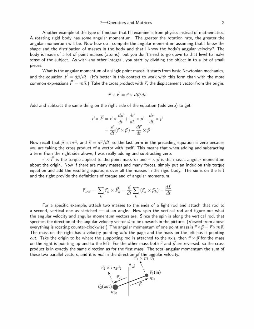
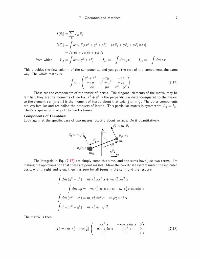
For a specific example, attach two masses to the ends of a light rod and attach that rod toa second, vertical one as sketched — at an angle. Now spin the vertical rod and figure out whatthe angular velocity and angular momentum vectors are. Since the spin is along the vertical rod, thatspecifies the direction of the angular velocity vector ~ω to be upwards in the picture. (Viewed from aboveeverything is rotating counter-clockwise.) The angular momentum of one point mass is ~r×~p = ~r×m~v.The mass on the right has a velocity pointing into the page and the mass on the left has it pointingout. Take the origin to be where the supporting rod is attached to the axis, then ~r × ~p for the masson the right is pointing up and to the left. For the other mass both ~r and ~p are reversed, so the crossproduct is in exactly the same direction as for the first mass. The total angular momentum the sum ofthese two parallel vectors, and it is not in the direction of the angular velocity.

~v2(out)

~r2 ×m2~v2

m2

~r2

~ω

~r1

~r1 ×m1~v1

~v1(in)

m1


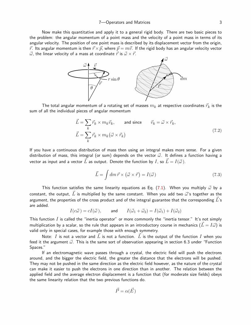
Now make this quantitative and apply it to a general rigid body. There are two basic pieces tothe problem: the angular momentum of a point mass and the velocity of a point mass in terms of itsangular velocity. The position of one point mass is described by its displacement vector from the origin,~r. Its angular momentum is then ~r×~p, where ~p = m~v. If the rigid body has an angular velocity vector~ω, the linear velocity of a mass at coordinate ~r is ~ω × ~r.

~ω

θ~r

~v

r sin θ

~r

~ω

dm

The total angular momentum of a rotating set of masses mk at respective coordinates ~rk is thesum of all the individual pieces of angular momentum

~L =∑k

~rk ×mk~vk, and since ~vk = ~ω × ~rk,

~L =∑k

~rk ×mk

(~ω × ~rk

) (7.2)

If you have a continuous distribution of mass then using an integral makes more sense. For a givendistribution of mass, this integral (or sum) depends on the vector ~ω. It defines a function having a

vector as input and a vector ~L as output. Denote the function by I , so ~L = I(~ω ).

~L =

∫dm~r ×

(~ω × ~r

)= I(~ω ) (7.3)

This function satisfies the same linearity equations as Eq. (7.1). When you multiply ~ω by a

constant, the output, ~L is multiplied by the same constant. When you add two ~ω’s together as the

argument, the properties of the cross product and of the integral guarantee that the corresponding ~L’sare added.

I(c~ω ) = cI(~ω ), and I(~ω1 + ~ω2) = I(~ω1) + I(~ω2)

This function I is called the “inertia operator” or more commonly the “inertia tensor.” It’s not simply

multiplication by a scalar, so the rule that appears in an introductory course in mechanics (~L = I~ω) isvalid only in special cases, for example those with enough symmetry.

Note: I is not a vector and ~L is not a function. ~L is the output of the function I when youfeed it the argument ~ω. This is the same sort of observation appearing in section 6.3 under “FunctionSpaces.”

If an electromagnetic wave passes through a crystal, the electric field will push the electronsaround, and the bigger the electric field, the greater the distance that the electrons will be pushed.They may not be pushed in the same direction as the electric field however, as the nature of the crystalcan make it easier to push the electrons in one direction than in another. The relation between theapplied field and the average electron displacement is a function that (for moderate size fields) obeysthe same linearity relation that the two previous functions do.

~P = α( ~E )


~P is the electric dipole moment density and ~E is the applied electric field. The function α is called thepolarizability.

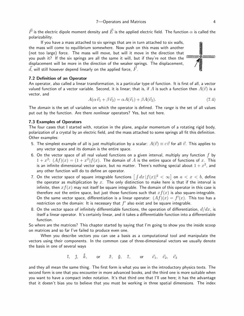
If you have a mass attached to six springs that are in turn attached to six walls,the mass will come to equilibrium somewhere. Now push on this mass with another(not too large) force. The mass will move, but will it move in the direction thatyou push it? If the six springs are all the same it will, but if they’re not then thedisplacement will be more in the direction of the weaker springs. The displacement,~d, will still however depend linearly on the applied force, ~F .

7.2 Definition of an OperatorAn operator, also called a linear transformation, is a particular type of function. It is first of all, a vectorvalued function of a vector variable. Second, it is linear; that is, if A is such a function then A(~v) is avector, and

A(α~v1 + β~v2) = αA(~v1) + βA(~v2). (7.4)

The domain is the set of variables on which the operator is defined. The range is the set of all valuesput out by the function. Are there nonlinear operators? Yes, but not here.

7.3 Examples of OperatorsThe four cases that I started with, rotation in the plane, angular momentum of a rotating rigid body,polarization of a crystal by an electric field, and the mass attached to some springs all fit this definition.Other examples:

5. The simplest example of all is just multiplication by a scalar: A(~v) ≡ c~v for all ~v. This applies toany vector space and its domain is the entire space.

6. On the vector space of all real valued functions on a given interval, multiply any function f by1 + x2: (Af)(x) = (1 + x2)f(x). The domain of A is the entire space of functions of x. Thisis an infinite dimensional vector space, but no matter. There’s nothing special about 1 + x2, andany other function will do to define an operator.

7. On the vector space of square integrable functions[ ∫

dx |f(x)|2 < ∞]

on a < x < b, definethe operator as multiplication by x. The only distinction to make here is that if the interval isinfinite, then xf(x) may not itself be square integrable. The domain of this operator in this case istherefore not the entire space, but just those functions such that xf(x) is also square-integrable.On the same vector space, differentiation is a linear operator: (Af)(x) = f ′(x). This too has arestriction on the domain: It is necessary that f ′ also exist and be square integrable.

8. On the vector space of infinitely differentiable functions, the operation of differentiation, d/dx, isitself a linear operator. It’s certainly linear, and it takes a differentiable function into a differentiablefunction.

So where are the matrices? This chapter started by saying that I’m going to show you the inside scoopon matrices and so far I’ve failed to produce even one.

When you describe vectors you can use a basis as a computational tool and manipulate thevectors using their components. In the common case of three-dimensional vectors we usually denotethe basis in one of several ways

ı, , k, or x, y, z, or ~e1, ~e2, ~e3

and they all mean the same thing. The first form is what you see in the introductory physics texts. Thesecond form is one that you encounter in more advanced books, and the third one is more suitable whenyou want to have a compact index notation. It’s that third one that I’ll use here; it has the advantagethat it doesn’t bias you to believe that you must be working in three spatial dimensions. The index


could go beyond 3, and the vectors that you’re dealing with may not be the usual geometric arrows.(And why does it have to start with one? Maybe I want the indices 0, 1, 2 instead.) These need notbe perpendicular to each other or even to be unit vectors.

The way to write a vector ~v in components is

~v = vx x+ vy y + vz z, or v1~e1 + v2~e2 + v3~e3 =∑k

vk~ek (7.5)

Once you’ve chosen a basis, you can find the three numbers that form the components of thatvector. In a similar way, define the components of an operator, only that will take nine numbers to doit (in three dimensions). If you evaluate the effect of an operator on any one of the basis vectors, theoutput is a vector. That’s part of the definition of the word operator. This output vector can itself bewritten in terms of this same basis. The defining equation for the components of an operator f is

f(~ei) =3∑k=1

fki~ek (7.6)

For each input vector you have the three components of the output vector. Pay careful attentionto this equation! It is the defining equation for the entire subject of matrix theory, and everything inthat subject comes from this one innocuous looking equation. (And yes if you’re wondering, I wrotethe indices in the correct order.)

Why?Take an arbitrary input vector for f : ~u = f(~v ). Both ~u and ~v are vectors, so write them in

terms of the basis chosen.

~u =∑k

uk~ek = f(~v ) = f(∑

i

vi~ei)

=∑i

vif(~ei) (7.7)

The last equation is the result of the linearity property, Eq. (7.1), already assumed for f . Now pull thesum and the numerical factors vi out in front of the function, and write it out. It is then clear:

f(v1~e1 + v2~e2) = f(v1~e1) + f(v2~e2) = v1f(~e1) + v2f(~e2)

Now you see where the defining equation for operator components comes in. Eq. (7.7) is∑k

uk~ek =∑i

vi∑k

fki~ek

For two vectors to be equal, the corresponding coefficients of ~e1, ~e2, etc. must match; their respectivecomponents must be equal, and this is

uk =∑i

vifki, usually written uk =∑i

fkivi (7.8)

so that in the latter form it starts to resemble what you may think of as matrix manipulation. frow,column

is the conventional way to write the indices, and multiplication is defined so that the following productmeans Eq. (7.8). u1u2

u3

=

f11 f12 f13f21 f22 f23f31 f32 f33

v1v2v3

(7.9)


u1u2u3

=

f11 f12 f13f21 f22 f23f31 f32 f33

v1v2v3

is u1 = f11v1 + f12v2 + f13v3 etc.

And this is the reason behind the definition of how to multiply a matrix and a column matrix. Theorder in which the indices appear is the conventional one, and the indices appear in the matrix as theydo because I chose the order of the indices in a (seemingly) backwards way in Eq. (7.6).

Components of RotationsApply this to the first example, rotate all vectors in the plane through the angle α. I don’t want tokeep using the same symbol f for every function, so I’ll call this function R instead, or better yet Rα.Rα(~v ) is the rotated vector. Pick two perpendicular unit vectors for a basis. You may call them x andy, but again I’ll call them ~e1 and ~e2. Use the definition of components to get

Rα(~e2)~e2

cosαα

Rα(~e1)

sinα

~e1

Rα(~e1) =∑k

Rk1~ek

Rα(~e2) =∑k

Rk2~ek(7.10)

The rotated ~e1 has two components, so

Rα(~e1) = ~e1 cosα+ ~e2 sinα = R11~e1 +R21~e2 (7.11)

This determines the first column of the matrix of components,

R11 = cosα, and R21 = sinα

Similarly the effect on the other basis vector determines the second column:

Rα(~e2) = ~e2 cosα− ~e1 sinα = R12~e1 +R22~e2 (7.12)

Check: Rα(~e1) .Rα(~e2) = 0.

R12 = − sinα, and R22 = cosα

The component matrix is then (Rα)

=

(cosα − sinαsinα cosα

)(7.13)

Components of InertiaThe definition, Eq. (7.3), and the figure preceding it specify the inertia tensor as the function thatrelates the angular momentum of a rigid body to its angular velocity.

~L =

∫dm~r ×

(~ω × ~r

)= I(~ω) (7.14)

Use the vector identity,~A× ( ~B × ~C ) = ~B( ~A . ~C )− ~C( ~A . ~B ) (7.15)

then the integral is

~L =

∫dm

[~ω(~r .~r )− ~r(~ω .~r )

]= I(~ω) (7.16)

Pick the common rectangular, orthogonal basis and evaluate the components of this function. Equa-tion (7.6) says ~r = x~e1 + y~e2 + z~e3 so


I(~ei) =∑k

Iki~ek

I(~e1) =

∫dm

[~e1(x

2 + y2 + z2)− (x~e1 + y~e2 + z~e3)(x)]

= I11~e1 + I21~e2 + I31~e3

from which I11 =

∫dm (y2 + z2), I21 = −

∫dmyx, I31 = −

∫dmzx

This provides the first column of the components, and you get the rest of the components the sameway. The whole matrix is ∫

dm

y2 + z2 −xy −xz−xy x2 + z2 −yz−xz −yz x2 + y2

(7.17)

These are the components of the tensor of inertia. The diagonal elements of the matrix may befamiliar; they are the moments of inertia. x2 + y2 is the perpendicular distance-squared to the z-axis,so the element I33 (≡ Izz) is the moment of inertia about that axis,

∫dmr2⊥. The other components

are less familiar and are called the products of inertia. This particular matrix is symmetric: Iij = Iji.That’s a special property of the inertia tensor.

Components of DumbbellLook again at the specific case of two masses rotating about an axis. Do it quantitatively.

~v2(out)

~r2 ×m2~v2

m2

~r2

~ω

~r1

~r1 ×m1~v1

~v1(in)

m1

~e2~e1

The integrals in Eq. (7.17) are simply sums this time, and the sums have just two terms. I’mmaking the approximation that these are point masses. Make the coordinate system match the indicatedbasis, with x right and y up, then z is zero for all terms in the sum, and the rest are∫

dm (y2 + z2) = m1r21 cos2 α+m2r

22 cos2 α

−∫dmxy = −m1r

21 cosα sinα−m2r

22 cosα sinα∫

dm (x2 + z2) = m1r21 sin2 α+m2r

22 sin2 α∫

dm (x2 + y2) = m1r21 +m2r

22

The matrix is then

(I ) =(m1r

21 +m2r

22

) cos2 α − cosα sinα 0− cosα sinα sin2 α 0

0 0 1

(7.18)


Don’t count on all such results factoring so nicely.

In this basis, the angular velocity ~ω has just one component, so what is ~L?

(m1r

21 +m2r

22

) cos2 α − cosα sinα 0− cosα sinα sin2 α 0

0 0 1

0ω0

=

(m1r

21 +m2r

22

)−ω cosα sinαω sin2 α

0

Translate this into vector form:

~L =(m1r

21 +m2r

22

)ω sinα

(− ~e1 cosα+ ~e2 sinα

)(7.19)

When α = 90◦, then cosα = 0 and the angular momentum points along the y-axis. This is thesymmetric special case where everything lines up along one axis. Notice that if α = 0 then everythingvanishes, but then the masses are both on the axis, and they have no angular momentum. In the general

case as drawn, the vector ~L points to the upper left, perpendicular to the line between the masses.

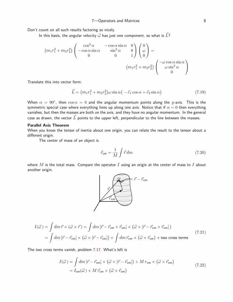
Parallel Axis TheoremWhen you know the tensor of inertia about one origin, you can relate the result to the tensor about adifferent origin.

The center of mass of an object is

~rcm =1

M

∫~r dm (7.20)

where M is the total mass. Compare the operator I using an origin at the center of mass to I aboutanother origin.

~r

~rcm

~r − ~rcm

I(~ω ) =

∫dm~r × (~ω × ~r ) =

∫dm [~r − ~rcm + ~rcm]×

(~ω × [~r − ~rcm + ~rcm]

)=

∫dm [~r − ~rcm]×

(~ω × [~r − ~rcm]

)+

∫dm~rcm ×

(~ω × ~rcm

)+ two cross terms

(7.21)

The two cross terms vanish, problem 7.17. What’s left is

I(~ω ) =

∫dm [~r − ~rcm]×

(~ω × [~r − ~rcm]

)+M rcm ×

(~ω × ~rcm

)= Icm(~ω ) +M ~rcm ×

(~ω × ~rcm

) (7.22)


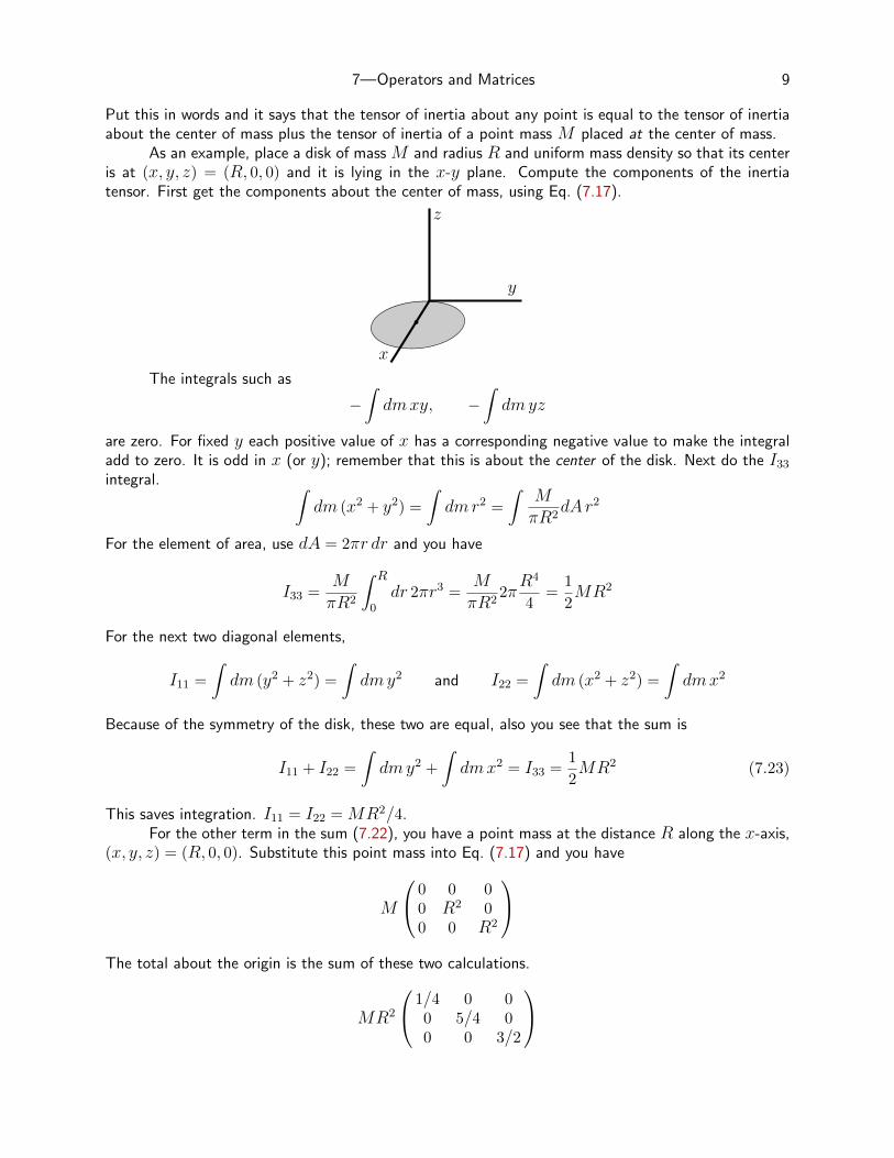
Put this in words and it says that the tensor of inertia about any point is equal to the tensor of inertiaabout the center of mass plus the tensor of inertia of a point mass M placed at the center of mass.

As an example, place a disk of mass M and radius R and uniform mass density so that its centeris at (x, y, z) = (R, 0, 0) and it is lying in the x-y plane. Compute the components of the inertiatensor. First get the components about the center of mass, using Eq. (7.17).

x

z

y

The integrals such as

−∫dmxy, −

∫dmyz

are zero. For fixed y each positive value of x has a corresponding negative value to make the integraladd to zero. It is odd in x (or y); remember that this is about the center of the disk. Next do the I33integral. ∫

dm (x2 + y2) =

∫dmr2 =

∫MπR2

dAr2

For the element of area, use dA = 2πr dr and you have

I33 =MπR2

∫ R

0dr 2πr3 =

MπR2

2πR4

4=

1

2MR2

For the next two diagonal elements,

I11 =

∫dm (y2 + z2) =

∫dmy2 and I22 =

∫dm (x2 + z2) =

∫dmx2

Because of the symmetry of the disk, these two are equal, also you see that the sum is

I11 + I22 =

∫dmy2 +

∫dmx2 = I33 =

1

2MR2 (7.23)

This saves integration. I11 = I22 = MR2/4.For the other term in the sum (7.22), you have a point mass at the distance R along the x-axis,

(x, y, z) = (R, 0, 0). Substitute this point mass into Eq. (7.17) and you have

M

0 0 00 R2 00 0 R2

The total about the origin is the sum of these two calculations.

MR2

1/4 0 00 5/4 00 0 3/2


Why is this called the parallel axis theorem when you’re translating a point (the origin) and not anaxis? Probably because this was originally stated for the moment of inertia alone and not for the wholetensor. In that case you have only an axis to deal with.

Components of the DerivativeThe set of all polynomials in x having degree ≤ 2 forms a vector space. There are three independentvectors that I can choose to be 1, x, and x2. Differentiation is a linear operator on this space becausethe derivative of a sum is the sum of the derivatives and the derivative of a constant times a functionis the constant times the derivative of the function. With this basis I’ll compute the components ofd/dx. Start the indexing for the basis from zero instead of one because it will cause less confusionbetween powers and subscripts.

~e0 = 1, ~e1 = x, ~e2 = x2

By the definition of the components of an operator — I’ll call this one D,

D(~e0) =ddx

1 = 0, D(~e1) =ddxx = 1 = ~e0, D(~e2) =

ddxx2 = 2x = 2~e1

These define the three columns of the matrix.

(D) =

0 1 00 0 20 0 0

check:dx2

dx= 2x is

0 1 00 0 20 0 0

001

=

020

There’s nothing here about the basis being orthonormal. It isn’t.

7.4 Matrix MultiplicationHow do you multiply two matrices? There’s a rule for doing it, but where does it come from?

The composition of two functions means you first apply one function then the other, so

h = f ◦ g means h(~v ) = f(g(~v )

)(7.24)

I’m assuming that these are vector-valued functions of a vector variable, but this is the general definitionof composition anyway. If f and g are linear, does it follow the h is? Yes, just check:

h(c~v ) = f(g(c~v )

)= f

(cg(~v )

)= c f

(g(~v )

), and

h(~v1 + ~v2) = f(g(~v1 + ~v2)

)= f

(g(~v1) + g(~v2)

)= f

(g(~v1)

)+ f

(g(~v2)

)What are the components of h? Again, use the definition and plug in.

h(~ei) =∑k

hki~ek = f(g(~ei)

)= f

(∑j

gji~ej)

=∑j

gjif(~ej)

=∑j

gji∑k

fkj~ek (7.25)

and now all there is to do is to equate the corresponding coefficients of ~ek.

hki =∑j

gjifkj or more conventionally hki =∑j

fkjgji (7.26)

This is in the standard form for matrix multiplication, recalling the subscripts are ordered as frc forrow-column. h11 h12 h13

h21 h32 h23h31 h32 h33

=

f11 f12 f13f21 f32 f23f31 f32 f33

g11 g12 g13g21 g32 g23g31 g32 g33

(7.27)


The computation of h12 from Eq. (7.26) ish11 h12 h13h21 h22 h23h31 h32 h33

=

f11 f12 f13f21 f22 f23f31 f32 f33

g11 g12 g13g21 g22 g23g31 g32 g33

−→ h12 = f11g12 + f12g22 + f13g32

Matrix multiplication is just the component representation of the composition of two functions,Eq. (7.26), and there’s nothing here that restricts this to three dimensions. In Eq. (7.25) I may havemade it look too easy. If you try to reproduce this without looking, the odds are that you will notget the indices to match up as nicely as you see there. Remember: When an index is summed it is adummy, and you are free to relabel it as anything you want. You can use this fact to make the indicescome out neatly.

Composition of RotationsIn the first example, rotating vectors in the plane, the operator that rotates every vector by the angleα has components (

Rα)

=


)(7.28)

What happens if you do two such transformations, one by α and one by β? The result better be a totalrotation by α+ β. One function, Rβ is followed by the second function Rα and the composition is

Rα+β = RαRβ

This is mirrored in the components of these operators, so the matrices must obey the same equation.(cos(α+ β) − sin(α+ β)sin(α+ β) cos(α+ β)

)=


)(cosβ − sinβsinβ cosβ

)Multiply the matrices on the right to get(

cosα cosβ − sinα sinβ − cosα sinβ − sinα cosβsinα cosβ + cosα sinβ cosα cosβ − sinα sinβ

)(7.29)

The respective components must agree, so this gives an immediate derivation of the formulas for thesine and cosine of the sum of two angles. Cf. Eq. (3.8)

7.5 InversesThe simplest operator is the one that does nothing. f(~v ) = ~v for all values of the vector ~v. This impliesthat f(~e1) = ~e1 and similarly for all the other elements of the basis, so the matrix of its componentsis diagonal. The 2× 2 matrix is explicitly the identity matrix

(I ) =

(1 00 1

)or in index notation δij =

{1 (if i = j)0 (if i 6= j)

(7.30)

and the index notation is completely general, not depending on whether you’re dealing with two dimen-sions or many more. Unfortunately the words “inertia” and “identity” both start with the letter “I” andthis symbol is used for both operators. Live with it. The δ symbol in this equation is the Kroneckerdelta — very handy.

The inverse of an operator is defined in terms of Eq. (7.24), the composition of functions. If thecomposition of two functions takes you to the identity operator, one function is said to be the inverse of


the other. This is no different from the way you look at ordinary real valued functions. The exponentialand the logarithm are inverse to each other because*

ln(ex) = x for all x.

For the rotation operator, Eq. (7.10), the inverse is obviously going to be rotation by the same anglein the opposite direction.

RαR−α = I

Because the matrix components of these operators mirror the original operators, this equation mustalso hold for the corresponding components, as in Eqs. (7.27) and (7.29). Set β = −α in (7.29) andyou get the identity matrix.

In an equation such as Eq. (7.7), or its component version Eqs. (7.8) or (7.9), if you want tosolve for the vector ~u, you are asking for the inverse of the function f .

~u = f(~v ) implies ~v = f−1(~u)

The translation of these equations into components is Eq. (7.9)(u1u2

)=

(f11 f12f21 f22

)(v1v2

)

which implies1

f11f22 − f12f21

(f22 −f12−f21 f11

)(u1u2

)=

(v1v2

)(7.31)

The verification that these are the components of the inverse is no more than simply multiplying thetwo matrices and seeing that you get the identity matrix.

7.6 Rotations, 3-dIn three dimensions there are of course more basis vectors to rotate. Start by rotating vectors aboutthe axes and it is nothing more than the two-dimensional problem of Eq. (7.10) done three times. Youdo have to be careful about signs, but not much more — as long as you draw careful pictures!

x

y

z

x

y

z

x

y

z

α

β

γ

The basis vectors are drawn in the three pictures: ~e1 = x, ~e2 = y, ~e3 = z.In the first sketch, rotate vectors by the angle α about the x-axis. In the second case, rotate by

the angle β about the y-axis, and in the third case, rotate by the angle γ about the z-axis. In the firstcase, the ~e1 is left alone. The ~e2 picks up a little positive ~e3, and the ~e3 picks up a little negative ~e2.

Rα~e1(~e1)

= ~e1, Rα~e1(~e2)

= ~e2 cosα+ ~e3 sinα, Rα~e1(~e3)

= ~e3 cosα− ~e2 sinα (7.32)

* The reverse, elnx works just for positive x, unless you recall that the logarithm of a negativenumber is complex. Then it works there too. This sort of question doesn’t occur with finite dimensionalmatrices.


Here the notation R~θ represents the function prescribing a rotation by θ about the axis pointing along

θ. These equations are the same as Eqs. (7.11) and (7.12).The corresponding equations for the other two rotations are now easy to write down:

Rβ~e2(~e1)

= ~e1 cosβ − ~e3 sinβ, Rβ~e2(~e2)

= ~e2, Rβ~e2(~e3)

= ~e1 sinβ + ~e3 cosβ (7.33)

Rγ~e3(~e1)

= ~e1 cos γ + ~e2 sin γ, Rγ~e3(~e2)

= −~e1 sin γ + ~e2 cos γ, Rγ~e3(~e3)

= ~e3 (7.34)

From these vector equations you immediate read the columns of the matrices of the components of theoperators as in Eq. (7.6).(

Rα~e1) (

Rβ~e2) (

Rγ~e3) 1 0 0

0 cosα − sinα0 sinα cosα

, cosβ 0 sinβ

0 1 0− sinβ 0 cosβ

, cos γ − sin γ 0

sin γ cos γ 00 0 1

(7.35)

As a check on the algebra, did you see if the rotated basis vectors from any of the three sets of equations(7.32)-(7.34) are still orthogonal sets?

Do these rotation operations commute? No. Try the case of two 90◦ rotations to see. Rotateby this angle about the x-axis then by the same angle about the y-axis.

(R~e2π/2

)(R~e1π/2

)=

0 0 10 1 0−1 0 0

1 0 00 0 −10 1 0

=

0 1 00 0 −1−1 0 0

(7.36)

In the reverse order, for which the rotation about the y-axis is done first, these are

(R~e1π/2

)(R~e2π/2

)=

1 0 00 0 −10 1 0

0 0 10 1 0−1 0 0

=

0 0 11 0 00 1 0

(7.37)

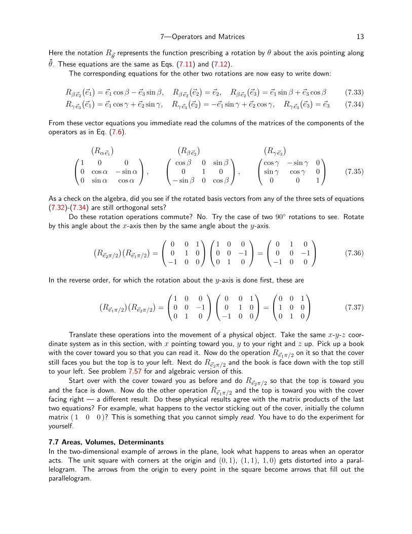
Translate these operations into the movement of a physical object. Take the same x-y-z coor-dinate system as in this section, with x pointing toward you, y to your right and z up. Pick up a bookwith the cover toward you so that you can read it. Now do the operation R~e1π/2 on it so that the cover

still faces you but the top is to your left. Next do R~e2π/2 and the book is face down with the top stillto your left. See problem 7.57 for and algebraic version of this.

Start over with the cover toward you as before and do R~e2π/2 so that the top is toward you

and the face is down. Now do the other operation R~e1π/2 and the top is toward you with the coverfacing right — a different result. Do these physical results agree with the matrix products of the lasttwo equations? For example, what happens to the vector sticking out of the cover, initially the columnmatrix ( 1 0 0 )? This is something that you cannot simply read. You have to do the experiment foryourself.

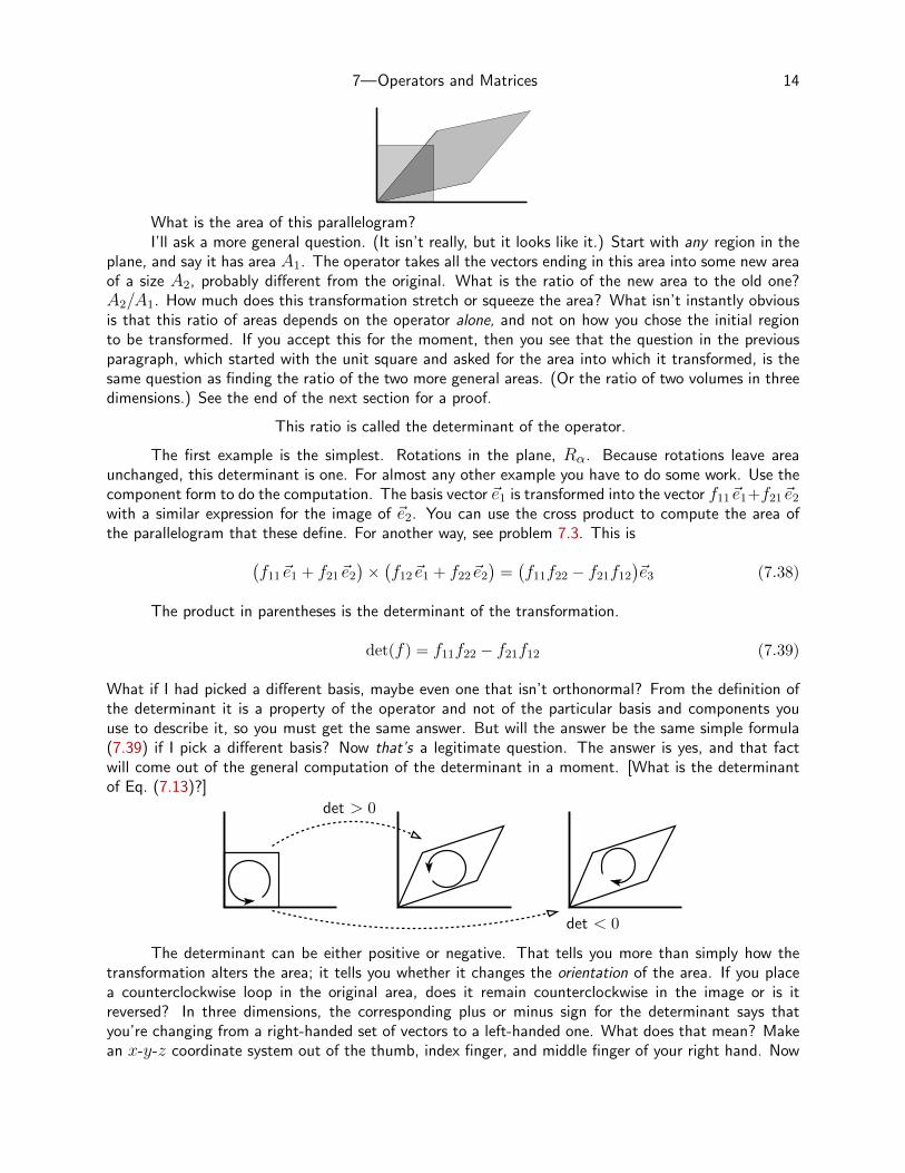
7.7 Areas, Volumes, DeterminantsIn the two-dimensional example of arrows in the plane, look what happens to areas when an operatoracts. The unit square with corners at the origin and (0, 1), (1, 1), 1, 0) gets distorted into a paral-lelogram. The arrows from the origin to every point in the square become arrows that fill out theparallelogram.


What is the area of this parallelogram?I’ll ask a more general question. (It isn’t really, but it looks like it.) Start with any region in the

plane, and say it has area A1. The operator takes all the vectors ending in this area into some new areaof a size A2, probably different from the original. What is the ratio of the new area to the old one?A2/A1. How much does this transformation stretch or squeeze the area? What isn’t instantly obviousis that this ratio of areas depends on the operator alone, and not on how you chose the initial regionto be transformed. If you accept this for the moment, then you see that the question in the previousparagraph, which started with the unit square and asked for the area into which it transformed, is thesame question as finding the ratio of the two more general areas. (Or the ratio of two volumes in threedimensions.) See the end of the next section for a proof.

This ratio is called the determinant of the operator.

The first example is the simplest. Rotations in the plane, Rα. Because rotations leave areaunchanged, this determinant is one. For almost any other example you have to do some work. Use thecomponent form to do the computation. The basis vector ~e1 is transformed into the vector f11~e1+f21~e2with a similar expression for the image of ~e2. You can use the cross product to compute the area ofthe parallelogram that these define. For another way, see problem 7.3. This is(

f11~e1 + f21~e2)×(f12~e1 + f22~e2

)=(f11f22 − f21f12

)~e3 (7.38)

The product in parentheses is the determinant of the transformation.

det(f) = f11f22 − f21f12 (7.39)

What if I had picked a different basis, maybe even one that isn’t orthonormal? From the definition ofthe determinant it is a property of the operator and not of the particular basis and components youuse to describe it, so you must get the same answer. But will the answer be the same simple formula(7.39) if I pick a different basis? Now that’s a legitimate question. The answer is yes, and that factwill come out of the general computation of the determinant in a moment. [What is the determinantof Eq. (7.13)?]

det > 0

det < 0

The determinant can be either positive or negative. That tells you more than simply how thetransformation alters the area; it tells you whether it changes the orientation of the area. If you placea counterclockwise loop in the original area, does it remain counterclockwise in the image or is itreversed? In three dimensions, the corresponding plus or minus sign for the determinant says thatyou’re changing from a right-handed set of vectors to a left-handed one. What does that mean? Makean x-y-z coordinate system out of the thumb, index finger, and middle finger of your right hand. Now


do it with your left hand. You cannot move one of these and put it on top of the other (unless youhave very unusual joints). One is a mirror image of the other.

The equation (7.39) is a special case of a rule that you’ve probably encountered elsewhere. Youcompute the determinant of a square array of numbers by some means such as expansion in minors orGauss reduction. Here I’ve defined the determinant geometrically, and it has no obvious relation thetraditional numeric definition. They are the same, and the reason for that comes by looking at how thearea (or volume) of a parallelogram depends on the vectors that make up its sides. The derivation isslightly involved, but no one step in it is hard. Along the way you will encounter a new and importantfunction: Λ.

Start with the basis ~e1, ~e2 and call the output of the transformation ~v1 = f(~e1) and ~v2 = f(~e2).The final area is a function of these last two vectors, call it Λ

(~v1,~v2

), and this function has two key

properties:

Λ(~v,~v

)= 0, and Λ

(~v1, α~v2 + β~v3

)= αΛ

(~v1,~v2

)+ βΛ

(~v1,~v3

)(7.40)

That the area vanishes if the two sides are the same is obvious. That the area is a linear function ofthe vectors forming the two sides is not so obvious. (It is linear in both arguments.) Part of the proofof linearity is easy:

Λ(~v1, α~v2) = αΛ

(~v1,~v2)

simply says that if one side of the parallelogram remains fixed and the other changes by some factor,then the area changes by that same factor. For the other part, Λ

(~v1,~v2 +~v3

), start with a picture and

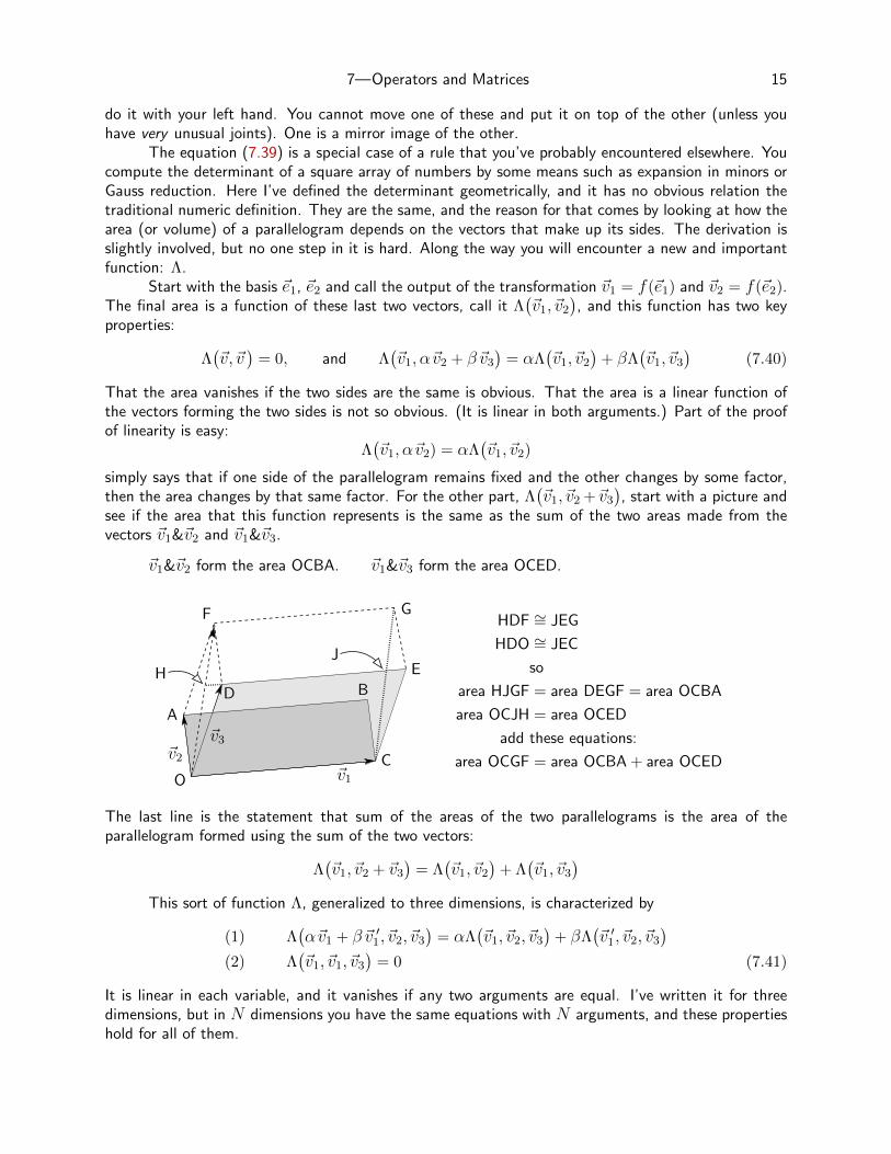
see if the area that this function represents is the same as the sum of the two areas made from thevectors ~v1&~v2 and ~v1&~v3.

~v1&~v2 form the area OCBA. ~v1&~v3 form the area OCED.

O

A

B

C

D

E

F G

HJ

~v1

~v2~v3

HDF ∼= JEG

HDO ∼= JEC

so

area HJGF = area DEGF = area OCBA

area OCJH = area OCED

add these equations:

area OCGF = area OCBA + area OCED

The last line is the statement that sum of the areas of the two parallelograms is the area of theparallelogram formed using the sum of the two vectors:

Λ(~v1,~v2 + ~v3

)= Λ

(~v1,~v2

)+ Λ

(~v1,~v3

)This sort of function Λ, generalized to three dimensions, is characterized by

(1) Λ(α~v1 + β~v ′1,~v2,~v3

)= αΛ

(~v1,~v2,~v3

)+ βΛ

(~v ′1,~v2,~v3

)(2) Λ

(~v1,~v1,~v3

)= 0 (7.41)

It is linear in each variable, and it vanishes if any two arguments are equal. I’ve written it for threedimensions, but in N dimensions you have the same equations with N arguments, and these propertieshold for all of them.


Theorem: Up to an overall constant factor, this function is unique.

An important result is that these assumptions imply the function is antisymmetric in any twoarguments. Proof:

Λ(~v1 + ~v2,~v1 + ~v2,~v3

)= 0 = Λ

(~v1,~v1,~v3

)+ Λ

(~v1,~v2,~v3

)+ Λ

(~v2,~v1,~v3

)+ Λ

(~v2,~v2,~v3

)This is just the linearity property. Now the left side, and the 1st and 4th terms on the right, are zerobecause two arguments are equal. The rest is

Λ(~v1,~v2,~v3

)+ Λ

(~v2,~v1,~v3

)= 0 (7.42)

and this says that interchanging two arguments of Λ changes the sign. (The reverse is true also. Assumeantisymmetry and deduce that it vanishes if two arguments are equal.)

I said that this function is unique up to a factor. Suppose that there are two of them: Λ and Λ′.Now show for some constant α, that Λ − αΛ′ is identically zero. To do this, take three independentvectors and evaluate the number Λ′

(~va,~vb,~vc

)There is some set of ~v ’s for which this is non-zero,

otherwise Λ′ is identically zero and that’s not much fun. Now consider

α =Λ(~va,~vb,~vc

)Λ′(~va,~vb,~vc

) and define Λ0 = Λ− αΛ′

This function Λ0 is zero for the special argument: (~va,~vb,~vc), and now I’ll show why it is zero for allarguments. That means that it is the zero function, and says that the two functions Λ and Λ′ areproportional.

The vectors (~va,~vb,~vc) are independent and there are three of them (in three dimensions). Theyare a basis. You can write any vector as a linear combination of these. E.g.

~v1 = A~va +B~vb and ~v2 = C~va +D~vb and

Put these (and let’s say ~vc) into Λ0.

Λ0

(~v1,~v2, vc

)= ACΛ0

(~va,~va,~vc

)+ADΛ0

(~va,~vb,~vc

)+BCΛ0

(~vb,~va,~vc

)+BDΛ0

(~vb,~vb,~vc

)All these terms are zero. Any argument that you put into Λ0 is a linear combination of ~va, ~vb, and ~vc,and that means that this demonstration extends to any set of vectors, which in turn means that Λ0

vanishes for any arguments. It is identically zero and that implies Λ and Λ′ are, up to a constant overallfactor, the same.

In N dimensions, a scalar-valued function of N vector variables,linear in each argument and antisymmetric under interchanging anypairs of arguments, is unique up to a factor.

I’ve characterized this volume function Λ by two simple properties, and surprisingly enough this isall you need to compute it in terms of the components of the operator! With just this much informationyou can compute the determinant of a transformation.

Recall: ~v1 has for its components the first column of the matrix for the components of f , and~v2 forms the second column. Adding any multiple of one vector to another leaves the volume alone.This is

Λ(~v1,~v2 + α~v1,~v3

)= Λ

(~v1,~v2,~v3

)+ αΛ

(~v1,~v1,~v3

)(7.43)


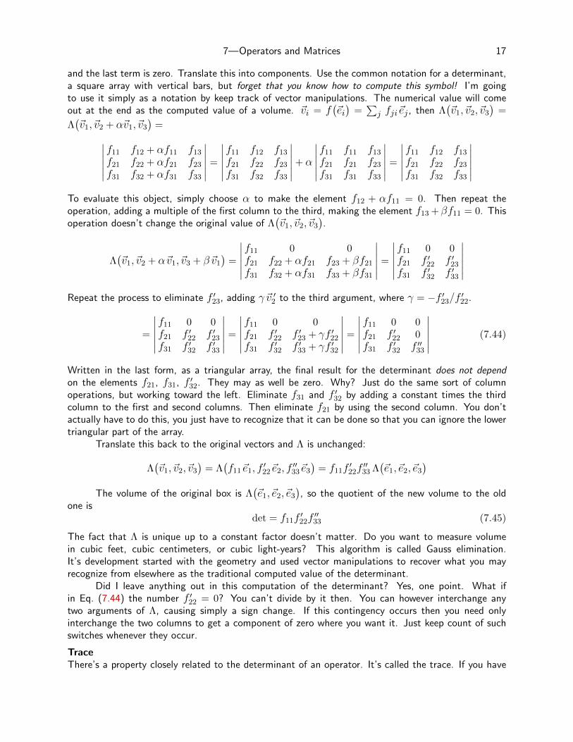
and the last term is zero. Translate this into components. Use the common notation for a determinant,a square array with vertical bars, but forget that you know how to compute this symbol! I’m goingto use it simply as a notation by keep track of vector manipulations. The numerical value will comeout at the end as the computed value of a volume. ~vi = f

(~ei)

=∑j fji~ej , then Λ

(~v1,~v2,~v3

)=

Λ(~v1,~v2 + α~v1,~v3

)=∣∣∣∣∣∣

f11 f12 + αf11 f13f21 f22 + αf21 f23f31 f32 + αf31 f33

∣∣∣∣∣∣ =

∣∣∣∣∣∣f11 f12 f13f21 f22 f23f31 f32 f33

∣∣∣∣∣∣+ α

∣∣∣∣∣∣f11 f11 f13f21 f21 f23f31 f31 f33

∣∣∣∣∣∣ =

∣∣∣∣∣∣f11 f12 f13f21 f22 f23f31 f32 f33

∣∣∣∣∣∣To evaluate this object, simply choose α to make the element f12 + αf11 = 0. Then repeat theoperation, adding a multiple of the first column to the third, making the element f13 +βf11 = 0. Thisoperation doesn’t change the original value of Λ

(~v1,~v2,~v3

).

Λ(~v1,~v2 + α~v1,~v3 + β~v1

)=

∣∣∣∣∣∣f11 0 0f21 f22 + αf21 f23 + βf21f31 f32 + αf31 f33 + βf31

∣∣∣∣∣∣ =

∣∣∣∣∣∣f11 0 0f21 f ′22 f ′23f31 f ′32 f ′33

∣∣∣∣∣∣Repeat the process to eliminate f ′23, adding γ~v ′2 to the third argument, where γ = −f ′23/f ′22.

=

∣∣∣∣∣∣f11 0 0f21 f ′22 f ′23f31 f ′32 f ′33

∣∣∣∣∣∣ =

∣∣∣∣∣∣f11 0 0f21 f ′22 f ′23 + γf ′22f31 f ′32 f ′33 + γf ′32

∣∣∣∣∣∣ =

∣∣∣∣∣∣f11 0 0f21 f ′22 0f31 f ′32 f ′′33

∣∣∣∣∣∣ (7.44)

Written in the last form, as a triangular array, the final result for the determinant does not dependon the elements f21, f31, f ′32. They may as well be zero. Why? Just do the same sort of columnoperations, but working toward the left. Eliminate f31 and f ′32 by adding a constant times the thirdcolumn to the first and second columns. Then eliminate f21 by using the second column. You don’tactually have to do this, you just have to recognize that it can be done so that you can ignore the lowertriangular part of the array.

Translate this back to the original vectors and Λ is unchanged:

Λ(~v1,~v2,~v3

)= Λ

(f11~e1, f

′22~e2, f

′′33~e3

)= f11f

′22f′′33 Λ

(~e1,~e2,~e3

)The volume of the original box is Λ

(~e1,~e2,~e3

), so the quotient of the new volume to the old

one isdet = f11f

′22f′′33 (7.45)

The fact that Λ is unique up to a constant factor doesn’t matter. Do you want to measure volumein cubic feet, cubic centimeters, or cubic light-years? This algorithm is called Gauss elimination.It’s development started with the geometry and used vector manipulations to recover what you mayrecognize from elsewhere as the traditional computed value of the determinant.

Did I leave anything out in this computation of the determinant? Yes, one point. What ifin Eq. (7.44) the number f ′22 = 0? You can’t divide by it then. You can however interchange anytwo arguments of Λ, causing simply a sign change. If this contingency occurs then you need onlyinterchange the two columns to get a component of zero where you want it. Just keep count of suchswitches whenever they occur.

TraceThere’s a property closely related to the determinant of an operator. It’s called the trace. If you have


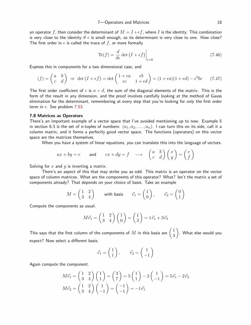
an operator f , then consider the determinant of M = I+εf , where I is the identity. This combinationis very close to the identity if ε is small enough, so its determinant is very close to one. How close?The first order in ε is called the trace of f , or more formally

Tr(f) =ddε

det(I + εf

)∣∣∣∣ε=0

(7.46)

Express this in components for a two dimensional case, and

(f) =

(a bc d

)⇒ det

(I + εf

)= det

(1 + εa εbεc 1 + εd

)= (1 + εa)(1 + εd)− ε2bc (7.47)

The first order coefficient of ε is a + d, the sum of the diagonal elements of the matrix. This is theform of the result in any dimension, and the proof involves carefully looking at the method of Gausselimination for the determinant, remembering at every step that you’re looking for only the first orderterm in ε. See problem 7.53.

7.8 Matrices as OperatorsThere’s an important example of a vector space that I’ve avoided mentioning up to now. Example 5in section 6.3 is the set of n-tuples of numbers: (a1, a2, . . . , an). I can turn this on its side, call it acolumn matrix, and it forms a perfectly good vector space. The functions (operators) on this vectorspace are the matrices themselves.

When you have a system of linear equations, you can translate this into the language of vectors.

ax+ by = e and cx+ dy = f −→(a bc d

)(xy

)=

(ef

)Solving for x and y is inverting a matrix.

There’s an aspect of this that may strike you as odd. This matrix is an operator on the vectorspace of column matrices. What are the components of this operator? What? Isn’t the matrix a set ofcomponents already? That depends on your choice of basis. Take an example

M =

(1 23 4

)with basis ~e1 =

(10

), ~e2 =

(01

)Compute the components as usual.

M~e1 =

(1 23 4

)(10

)=

(13

)= 1~e1 + 3~e2

This says that the first column of the components of M in this basis are

(13

). What else would you

expect? Now select a different basis.

~e1 =

(11

), ~e2 =

(1−1

)Again compute the component.

M~e1 =

(1 23 4

)(11

)=

(37

)= 5

(11

)− 2

(1−1

)= 5~e1 − 2~e2

M~e2 =

(1 23 4

)(1−1

)=

(−1−1

)= −1~e1


The components of M in this basis are

(5 −1−2 0

)It doesn’t look at all the same, but it represents the same operator. Does this matrix have the samedeterminant, using Eq. (7.39)?

Determinant of CompositionIf you do one linear transformation followed by another one, that is the composition of the two functions,each operator will then have its own determinant. What is the determinant of the composition? Letthe operators be F and G. One of them changes areas by a scale factor det(F ) and the other ratio ofareas is det(G). If you use the composition of the two functions, FG or GF , the overall ratio of areasfrom the start to the finish will be the same:

det(FG) = det(F ) . det(G) = det(G) . det(F ) = det(GF ) (7.48)

Recall that the determinant measures the ratio of areas for any input area, not just a square; it can bea parallelogram. The overall ratio of the product of the individual ratios, det(F ) det(G). The productof these two numbers is the total ratio of a new area to the original area and it is independent of theorder of F and G, so the determinant of the composition of the functions is also independent of order.

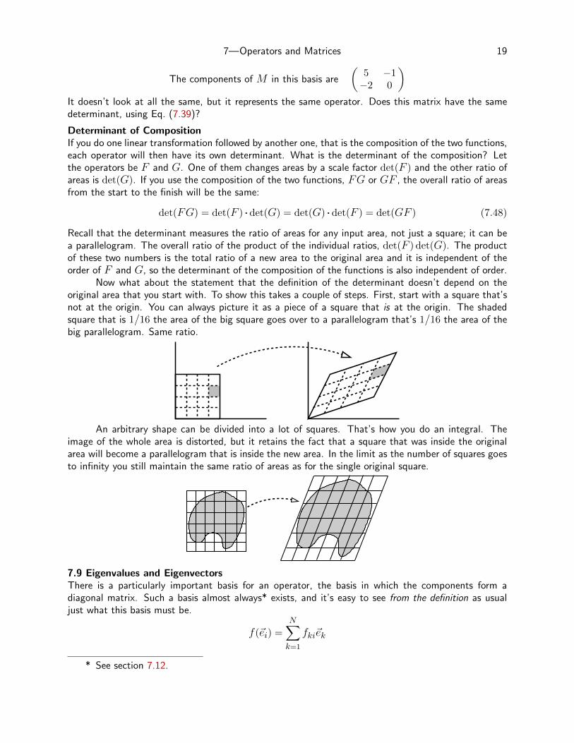
Now what about the statement that the definition of the determinant doesn’t depend on theoriginal area that you start with. To show this takes a couple of steps. First, start with a square that’snot at the origin. You can always picture it as a piece of a square that is at the origin. The shadedsquare that is 1/16 the area of the big square goes over to a parallelogram that’s 1/16 the area of thebig parallelogram. Same ratio.

An arbitrary shape can be divided into a lot of squares. That’s how you do an integral. Theimage of the whole area is distorted, but it retains the fact that a square that was inside the originalarea will become a parallelogram that is inside the new area. In the limit as the number of squares goesto infinity you still maintain the same ratio of areas as for the single original square.

7.9 Eigenvalues and EigenvectorsThere is a particularly important basis for an operator, the basis in which the components form adiagonal matrix. Such a basis almost always* exists, and it’s easy to see from the definition as usualjust what this basis must be.

f(~ei) =N∑k=1

fki~ek

* See section 7.12.


To be diagonal simply means that fki = 0 for all i 6= k, and that in turn means that all but one termin the sum disappears. This defining equation reduces to

f(~ei) = fii~ei (with no sum this time) (7.49)

This is called an eigenvalue equation. It says that for any one of these special vectors, the operator fon it returns a scalar multiple of that same vector. These multiples are called the eigenvalues, and thecorresponding vectors are called the eigenvectors. The eigenvalues are then the diagonal elements ofthe matrix in this basis.

The inertia tensor is the function that relates the angular momentum of a rigid body to itsangular velocity. The axis of rotation is defined by those points in the rotating body that aren’t moving,and the vector ~ω lies along that line. The angular momentum is computed from Eq. (7.3) and whenyou’ve done all those vector products and integrals you can’t really expect the angular momentum toline up with ~ω unless there is some exceptional reason for it. As the body rotates around the ~ω axis,~L will be carried with it, making ~L rotate about the direction of ~ω. The vector ~L is time-dependent

and that implies there will be a torque necessary to keep it going, ~τ = d~L/dt. Because ~L is rotatingwith frequency ω, this rotating torque will be felt as a vibration at this rotation frequency. If howeverthe angular momentum happens to be parallel to the angular velocity, the angular momentum will not

be changing; d~L/dt = 0 and the torque ~τ = d~L/dt will be zero, implying that the vibrations will beabsent. Have you ever taken your car in for servicing and asked the mechanic to make the angularmomentum and the angular velocity vectors of the wheels parallel? It’s called wheel-alignment.

How do you compute these eigenvectors? Just move everything to the left side of the precedingequation.

f(~ei)− fii~ei = 0, or (f − fiiI)~ei = 0

I is the identity operator, output equals input. This notation is cumbersome. I’ll change it.

f(~v ) = λ~v ↔ (f − λI)~v = 0 (7.50)

λ is the eigenvalue and ~v is the eigenvector. This operator (f − λI) takes some non-zero vector intothe zero vector. In two dimensions then it will squeeze an area down to a line or a point. In threedimensions it will squeeze a volume down to an area (or a line or a point). In any case the ratio of thefinal area (or volume) to the initial area (or volume) is zero. That says the determinant is zero, andthat’s the key to computing the eigenvectors. Figure out which λ’s will make this determinant vanish.

Look back at section 4.9 and you’ll see that the analysis there closely parallels what I’m doinghere. In that case I didn’t use the language of matrices or operators, but was asking about the possiblesolutions of two simultaneous linear equations.

ax+ by = 0 and cx+ dy = 0, or

(a bc d

)(xy

)=

(00

)The explicit algebra there led to the conclusion that there can be a non-zero solution (x, y) to the twoequations only if the determinant of the coefficients vanishes, ad− bc = 0, and that’s the same thingthat I’m looking for here: a non-zero vector solution to Eq. (7.50).

Write the problem in terms of components, and of course you aren’t yet in the basis where thematrix is diagonal. If you were, you’re already done. The defining equation is f(~v ) = λ~v, and incomponents this reads

∑i

fkivi = λvk, or

f11 f12 f13f21 f22 f23f31 f32 f33

v1v2v3

= λ

v1v2v3


Here I arbitrarily wrote the equation for three dimensions. That will change with the problem. Puteverything on the left side and insert the components of the identity, the unit matrix. f11 f12 f13

f21 f22 f23f31 f32 f33

− λ 1 0 0

0 1 00 0 1

v1v2v3

=

000

(7.51)

The one way that this has a non-zero solution for the vector ~v is for the determinant of the whole matrixon the left-hand side to be zero. This equation is called the characteristic equation of the matrix, and inthe example here that’s a cubic equation in λ. If it has all distinct roots, no double roots, then you’reguaranteed that this procedure will work, and you will be able to find a basis in which the componentsform a diagonal matrix. If this equation has a multiple root then there is no guarantee. It may work, butit may not; you have to look closer. See section 7.12. If the operator has certain symmetry propertiesthen it’s guaranteed to work. For example, the symmetry property found in problem 7.16 is enoughto insure that you can find a basis in which the matrix for the inertia tensor is diagonal. It is even anorthogonal basis in that case.

Example of EigenvectorsTo keep the algebra to a minimum, I’ll work in two dimensions and will specify an arbitrary but simpleexample:

f(~e1) = 2~e1 + ~e2, f (~e2) = 2~e2 + ~e1 with components M =

(2 11 2

)(7.52)

The eigenvalue equation is, in component form(2 11 2

)(v1v2

)= λ

(v1v2

)or

[(2 11 2

)− λ

(1 00 1

)](v1v2

)= 0 (7.53)

The condition that there be a non-zero solution to this is

det

[(2 11 2

)− λ

(1 00 1

)]= 0 = (2− λ)2 − 1

The solutions to this quadratic are λ = 1, 3. For these values then, the apparently two equation forthe two unknowns v1 and v2 are really one equation. The other is not independent. Solve this singleequation in each case. Take the first of the two linear equations for v1 and v2 as defined by Eq. (7.53).

2v1 + v2 = λv1λ = 1 implies v2 = −v1, λ = 3 implies v2 = v1

The two new basis vectors are then

~e ′1 = (~e1 − ~e2) and ~e ′2 = (~e1 + ~e2) (7.54)

and in this basis the matrix of components is the diagonal matrix of eigenvalues.(1 00 3

)If you like to keep your basis vectors normalized, you may prefer to say that the new basis is (~e1−~e2)/

√2

and (~e1 + ~e2)/√

2. The eigenvalues are the same, so the new matrix is the same.


Example: Coupled OscillatorsAnother example drawn from physics: Two masses are connected to a set of springs and fastenedbetween two rigid walls. This is a problem that appeared in chapter 4, Eq. (4.45).

m1d2x1/dt

2 = −k1x1 − k3(x1 − x2), and m2d2x2/dt

2 = −k2x2 − k3(x2 − x1)

The exponential form of the solution was

x1(t) = Aeiωt, x2(t) = Beiωt

The algebraic equations that you get by substituting these into the differential equations are apair of linear equations for A and B, Eq. (4.47). In matrix form these equations are, after rearrangingsome minus signs, (

k1 + k3 −k3−k3 k2 + k3

)(AB

)= ω2

(m1 00 m2

)(AB

)You can make it look more like the previous example with some further arrangement[(

k1 + k3 −k3−k3 k2 + k3

)− ω2

(m1 00 m2

)](AB

)=

(00

)The matrix on the left side maps the column matrix to zero. That can happen only if the matrix haszero determinant (or the column matrix is zero). If you write out the determinant of this 2× 2 matrixyou have a quadratic equation in ω2. It’s simple but messy, so rather than looking first at the generalcase, look at a special case with more symmetry. Take m1 = m2 = m and k1 = k2.

det

[(k1 + k3 −k3−k3 k1 + k3

)− ω2m

(1 00 1

)]= 0 =

(k1 + k3 −mω2

)2 − k23This is now so simple that you don’t even need the quadratic formula; it factors directly.(

k1 + k3 −mω2 − k3)(k1 + k3 −mω2 + k3

)= 0

The only way that the product of two numbers is zero is if one of the numbers is zero, so either

k1 −mω2 = 0 or k1 + 2k3 −mω2 = 0

This determines two possible frequencies of oscillation.

ω1 =

√k1m

and ω2 =

√k1 + 2k3m

You’re not done yet; these are just the eigenvalues. You still have to find the eigenvectors and then go

back to apply them to the original problem. This is ~F = m~a after all. Look back to section 4.10 forthe development of the solutions.


7.10 Change of BasisIn many problems in physics and mathematics, the correct choice of basis can enormously simplify aproblem. Sometimes the obvious choice of a basis turns out in the end not to be the best choice, andyou then face the question: Do you start over with a new basis, or can you use the work that you’vealready done to transform everything into the new basis?

For linear transformations, this becomes the problem of computing the components of an operatorin a new basis in terms of its components in the old basis.

First: Review how to do this for vector components, something that ought to be easy to do. Theequation (7.5) defines the components with respect to a basis, any basis. If I have a second proposedbasis, then by the definition of the word basis, every vector in that second basis can be written as alinear combination of the vectors in the first basis. I’ll call the vectors in the first basis, ~ei and those inthe second basis ~e ′i, for example in the plane you could have

~e1 = x, ~e2 = y, and ~e ′1 = 2 x+ 0.5 y, ~e ′2 = 0.5 x+ 2 y (7.55)

Each vector ~e ′i is a linear combination* of the original basis vectors:

~e ′i = S(~ei) =∑j

Sji~ej (7.56)

This follows the standard notation of Eq. (7.6); you have to put the indices in this order in order tomake the notation come out right in the end. One vector expressed in two different bases is still onevector, so

~v =∑i

v′i~e′i =

∑i

vi~ei

and I’m using the fairly standard notation of v′i for the ith component of the vector ~v with respect tothe second basis. Now insert the relation between the bases from the preceding equation (7.56).

~v =∑i

v′i∑j

Sji~ej =∑j

vj~ej

and this used the standard trick of changing the last dummy label of summation from i to j so that itis easy to compare the components.∑

i

Sjiv′i = vj or in matrix notation (S)(v′) = (v), =⇒ (v′) = (S)−1(v)

Similarity TransformationsNow use the definition of the components of an operator to get the components in the new basis.

f(~e ′i)

= =∑j

f ′ji~e′j

f(∑

j

Sji~ej)

=∑j

Sjif(~ej)

=∑j

Sji∑k

fkj~ek =∑j

f ′ji∑k

Skj~ek

* There are two possible conventions here. You can write ~e ′i in terms of the ~ei, calling thecoefficients Sji, or you can do the reverse and call those components Sji. [~ei = S(~e ′i)] Naturally, bothconventions are in common use. The reverse convention will interchange the roles of the matrices Sand S−1 in what follows.


The final equation comes from the preceding line. The coefficients of ~ek must agree on the two sidesof the equation. ∑

j

Sjifkj =∑j

f ′jiSkj

Now rearrange this in order to place the indices in their conventional row,column order.∑j

Skjf′ji =

∑j

fkjSji(S11 S12

S21 S22

)(f ′11 f ′12f ′21 f ′22

)=

(f11 f12f21 f22

)(S11 S12

S21 S22

) (7.57)

In turn, this matrix equation is usually written in terms of the inverse matrix of S,

(S)(f ′) = (f)(S) is (f ′) = (S)−1(f)(S) (7.58)

and this is called a similarity transformation. For the example Eq. (7.55) this is

~e ′1 = 2 x+ 0.5 y = S11~e1 + S21~e2

which determines the first column of the matrix (S), then ~e ′2 determines the second column.

(S) =

(2 0.5

0.5 2

)then (S)−1 =

1

3.75

(2 −0.5−0.5 2

)

EigenvectorsIn defining eigenvalues and eigenvectors I pointed out the utility of having a basis in which the com-ponents of an operator form a diagonal matrix. Finding the non-zero solutions to Eq. (7.50) is thenthe way to find the basis in which this holds. Now I’ve spent time showing that you can find a matrixin a new basis by using a similarity transformation. Is there a relationship between these two subjects?Another way to ask the question: I’ve solved the problem to find all the eigenvectors and eigenvalues,so what is the similarity transformation that accomplishes the change of basis (and why is it necessaryto know it if I already know that the transformed, diagonal matrix is just the set of eigenvalues, and Ialready know them)?

For the last question, the simplest answer is that you don’t need to know the explicit transforma-tion once you already know the answer. It is however useful to know that it exists and how to constructit. If it exists — I’ll come back to that presently. Certain manipulations are more easily done in termsof similarity transformations, so you ought to know how they are constructed, especially because almostall the work in constructing them is done when you’ve found the eigenvectors.

The equation (7.57) tells you the answer. Suppose that you want the transformed matrix to bediagonal. That means that f ′12 = 0 and f ′21 = 0. Write out the first column of the product on theright. (

f11 f12f21 f22

)(S11 S12

S21 S22

)−→

(f11 f12f21 f22

)(S11

S21

)This equals the first column on the left of the same equation

f ′11

(S11

S21

)


This is the eigenvector equation that you’ve supposedly already solved. The first column of the com-ponent matrix of the similarity transformation is simply the set of components of the first eigenvector.When you write out the second column of Eq. (7.57) you’ll see that it’s the defining equation for thesecond eigenvector. You already know these, so you can immediately write down the matrix for thesimilarity transformation.

For the example Eq. (7.52) the eigenvectors are given in Eq. (7.54). In components these are

~e ′1 →(

1−1

), and ~e ′2 →

(11

), implying S =

(1 1−1 1

)The inverse to this matrix is

S−1 =1

2

(1 −11 1

)You should verify that S−1MS is diagonal.

7.11 Summation ConventionIn all the manipulation of components of vectors and components of operators you have to do a lot ofsums. There are so many sums over indices that a convention* was invented (by Einstein) to simplifythe notation.

A repeated index in a term is summed.

Eq. (7.6) becomes f(~ei) = fki~ek.Eq. (7.8) becomes uk = fkivi.Eq. (7.26) becomes hki = fkjgji.IM = M becomes δijMjk = Mik.

What if there are three identical indices in the same term? Then you made a mistake; that can’thappen. What about Eq. (7.49)? That has three indices. Yes, and there I explicitly said that there isno sum. This sort of rare case you have to handle as an exception.

7.12 Can you Diagonalize a Matrix?At the beginning of section 7.9 I said that the basis in which the components of an operator form adiagonal matrix “almost always exists.” There’s a technical sense in which this is precisely true, butthat’s not what you need to know in order to manipulate matrices; the theorem that you need to haveis that every matrix is the limit of a sequence of diagonalizable matrices. If you encounter a matrix thatcannot be diagonalized, then you can approximate it as closely as you want by a matrix that can bediagonalized, do your calculations, and finally take a limit. You already did this if you did problem 4.11,but in that chapter it didn’t look anything like a problem involving matrices, much less diagonalizationof matrices. Yet it is the same.

Take the matrix (1 20 1

)You can’t diagonalize this. If you try the standard procedure, here is what happens:(

1 20 1

)(v1v2

)= λ

(v1v2

)then det

(1− λ 2

0 1− λ

)= 0 = (1− λ)2

The resulting equations you get for λ = 1 are

0v1 + 2v2 = 0 and 0 = 0

* There is a modification of this convention that appears in chapter 12, section 12.5


This provides only one eigenvector, a multiple of

(10

). You need two for a basis.

Change this matrix in any convenient way to make the two roots of the characteristic equationdifferent from each other. For example,

Mε =

(1 + ε 2

0 1

)The eigenvalue equation is now

(1 + ε− λ)(1− λ) = 0

and the resulting equations for the eigenvectors are

λ = 1 : εv1 + 2v2 = 0, 0 = 0 λ = 1 + ε : 0v1 + 2v2 = 0, εv2 = 0

Now you have two distinct eigenvectors,

λ = 1 :

(1−ε/2

), and λ = 1 + ε :

(10

)You see what happens to these vectors as ε→ 0.

Differential Equations at CriticalProblem 4.11 was to solve the damped harmonic oscillator for the critical case that b2 − 4km = 0.

md2xdt2

= −kx− bdxdt

(7.59)

Write this as a pair of equations, using the velocity as an independent variable.

dxdt

= vx anddvxdt

= − kmx− b

mvx

In matrix form, this is a matrix differential equation.

ddt

(xvx

)=

(0 1

−k/m −b/m

)(xvx

)This is a linear, constant-coefficient differential equation, but now the constant coefficients are matrices.Don’t let that slow you down. The reason that an exponential form of solution works is that thederivative of an exponential is an exponential. Assume such a solution here.(

xvx

)=

(AB

)eαt, giving α

(AB

)eαt =

(0 1

−k/m −b/m

)(AB

)eαt (7.60)

When you divide the equation by eαt, you’re left with an eigenvector equation where the eigenvalueis α. As usual, to get a non-zero solution set the determinant of the coefficients to zero and thecharacteristic equation is

det

(0− α 1−k/m −b/m− α

)= α(α+ b/m) + k/m = 0


with familiar rootsα =

(− b±

√b2 − 4km

)/2m

If the two roots are equal you may not have distinct eigenvectors, and in this case you do not. Nomatter, you can solve any such problem for the case that b2− 4km 6= 0 and then take the limit as thisapproaches zero.

The eigenvectors come from the either one of the two equations represented by Eq. (7.60). Pick

the simpler one, αA = B. The column matrix

(AB

)is then A

(1α

).

(xvx

)(t) = A+

(1α+

)eα+t +A−

(1α−

)eα−t

Pick the initial conditions that x(0) = 0 and vx(0) = v0. You must choose some initial conditions inorder to apply this technique. In matrix terminology this is(

0v0

)= A+

(1α+

)+A−

(1α−

)These are two equations for the two unknowns

A+ +A− = 0, α+A+ + α−A− = v0, so A+ =v0

α+ − α−, A− = −A+

(xvx

)(t) =

v0α+ − α−

[(1α+

)eα+t −

(1α−

)eα−t

]If you now take the limit as b2 → 4km, or equivalently as α− → α+, this expression is just the definitionof a derivative. (

xvx

)(t) −→ v0

ddα

(1α

)eαt = v0

(teαt

(1 + αt)eαt

)α = − b

2m(7.61)

7.13 Eigenvalues and GoogleThe motivating idea behind the search engine Google is that you want the first items returned by asearch to be the most important items. How do you do this? How do you program a computer todecide which web sites are the most important?

A simple idea is to count the number of sites that contain a link to a given site, and the site thatis linked to the most is then the most important site. This has the drawback that all links are treatedas equal. If your site is referenced from the home page of Al Einstein, it counts no more than if it’sreferenced by Joe Blow. This shouldn’t be.

A better idea is to assign each web page a numerical importance rating. If your site, #1, islinked from sites #11, #59, and #182, then your rating, x1, is determined by adding those ratings(and multiplying by a suitable scaling constant).

x1 = C(x11 + x59 + x182

)Similarly the second site’s rating is determined by what links to it, as

x2 = C(x137 + x157983 + x1 + x876

)


But this assumes that you already know the ratings of the sites, and that’s what you’re trying to find!Write this in matrix language. Each site is an element in a huge column matrix {xi}.

xi = CN∑j=1

αijxj or

x1x2...

= C

0 0 1 0 1 . . .1 0 0 0 0 . . .0 1 0 1 1 . . .. . .

x1x2

...

An entry of 1 indicates a link and a 0 is no link. This is an eigenvector problem with the eigenvalueλ = 1/C, and though there are many eigenvectors, there is a constraint that lets you pick the rightone. All the xis must be non-negative, and there’s a theorem (Perron-Frobenius) guaranteeing thatyou can find such an eigenvector. This algorithm is a key idea behind Google’s ranking methods. Theyhave gone well beyond this basic technique of course, but the spirit of the method remains.

See www-db.stanford.edu/˜backrub/google.html for more on this.

7.14 Special OperatorsSymmetricAntisymmetricHermitianAntihermitianOrthogonalUnitaryIdempotentNilpotentSelf-adjoint

In no particular order of importance, these are names for special classes of operators. It is oftenthe case that an operator defined in terms of a physical problem will be in some way special, and it’sthen worth knowing the consequent simplifications. The first ones involve a scalar product.

Symmetric:⟨~u, S(~v )

⟩=⟨S(~u ),~v

⟩Antisymmetric:

⟨~u,A(~v )

⟩= −

⟨A(~u ),~v

⟩The inertia operator of Eq. (7.3) is symmetric.

I(~ω ) =

∫dm~r ×

(~ω × ~r

)satisfies

⟨~ω1, I(~ω2)

⟩= ~ω1 . I(~ω2) =

⟨I(~ω1), ~ω2

⟩= I(~ω1) . ~ω2

Proof: Plug in.

~ω1 . I(~ω2) = ~ω1 .∫dm~r ×

(~ω2 × ~r

)= ~ω1 .

∫dm

[~ω2 r

2 − ~r (~ω2 .~r )]

=

∫dm

[~ω1 . ~ω2 r

2 − (~ω1 .~r )(~ω2 .~r )]

= I(~ω1) . ~ω2

What good does this do? You will be guaranteed that all eigenvalues are real, all eigenvectors areorthogonal, and the eigenvectors form an orthogonal basis. In this example, the eigenvalues are momentsof inertia about the axes defined by the eigenvectors, so these moments better be real. The magneticfield operator (problem 7.28) is antisymmetric.

Hermitian operators obey the same identity as symmetric:⟨~u,H(~v )

⟩=⟨H(~u ),~v

⟩. The

difference is that in this case you allow the scalars to be complex numbers. That means that the scalarproduct has a complex conjugation implied in the first factor. You saw this sort of operator in the

http://www-db.stanford.edu/~backrub/google.html


chapter on Fourier series, section 5.3, but it didn’t appear under this name. You will become familiarwith this class of operators when you hit quantum mechanics. Then they are ubiquitous. The sametheorem as for symmetric operators applies here, that the eigenvalues are real and that the eigenvectorsare orthogonal.

Orthogonal operators satisfy⟨O(~u ),O(~v )

⟩=⟨~u,~v

⟩. The most familiar example is rotation.

When you rotate two vectors, their magnitudes and the angle between them do not change. That’s allthat this equation says — scalar products are preserved by the transformation.

Unitary operators are the complex analog of orthogonal ones:⟨U(~u), U(~v )

⟩=⟨~u,~v

⟩, but all

the scalars are complex and the scalar product is modified accordingly.The next couple you don’t see as often. Idempotent means that if you take the square of the

operator, it equals the original operator.Nilpotent means that if you take successive powers of the operator you eventually reach the

zero operator.Self-adjoint in a finite dimensional vector space is exactly the same thing as Hermitian. In

infinite dimensions it is not, and in quantum mechanics the important operators are the self-adjointones. The issues involved are a bit technical. As an aside, in infinite dimensions you need one extrahypothesis for unitary and orthogonal: that they are invertible.


Problems

7.1 Draw a picture of the effect of these linear transformations on the unit square with vertices at(0, 0), (1, 0), (1, 1), (0, 1). The matrices representing the operators are

(a)

(1 23 4

), (b)

(1 −22 −4

), (c)

(−1 21 2

)Is the orientation preserved or not in each case? See the figure at the end of section 7.7

7.2 Using the same matrices as the preceding question, what is the picture resulting from doing (a)followed by (c)? What is the picture resulting from doing (c) followed by (a)? The results of section7.4 may prove helpful.

(a, c)

(b, d)

(a+ b, c+ d)7.3 Look again at the parallelogram that is the image of the unit square inthe calculation of the determinant. In Eq. (7.39) I used the cross product toget its area, but sometimes a brute-force method is more persuasive. If the

transformation has components

(a bc d

)The corners of the parallelogram

that is the image of the unit square are at (0, 0), (a, c), (a + b, c + d),(b, d). You can compute its area as sums and differences of rectangles andtriangles. Do so; it should give the same result as the method that used across product.

7.4 In three dimensions, there is an analogy to the geometric interpretation of the cross product as the

area of a parallelogram. The triple scalar product ~A . ~B × ~C is the volume of the parallelepiped havingthese three vectors as edges. Prove both of these statements starting from the geometric definitionsof the two products. That is, from the AB cos θ and AB sin θ definitions of the dot product and themagnitude of the cross product (and its direction).

7.5 Derive the relation ~v = ~ω × ~r for a point mass rotating about an axis. Refer to the figure beforeEq. (7.2).

7.6 You have a mass attached to four springs in a plane and that are in turn attached to four walls ason page 3; the mass is at equilibrium. Two opposing spring have spring constant k1 and the other two

are k2. Push on the mass with a (small) force ~F and the resulting displacement of m is ~d = f(~F ),defining a linear operator. Compute the components of f in an obvious basis and check a couple ofspecial cases to see if the displacement is in a plausible direction, especially if the two k’s are quitedifferent.

7.7 On the vector space of quadratic polynomials, degree ≤ 2, the operator d/dx is defined: thederivative of such a polynomial is a polynomial. (a) Use the basis ~e0 = 1, ~e1 = x, and ~e2 = x2

and compute the components of this operator. (b) Compute the components of the operator d2/dx2.(c) Compute the square of the first matrix and compare it to the result for (b). Ans: (a)2 = (b)

7.8 Repeat the preceding problem, but look at the case of cubic polynomials, a four-dimensional space.

7.9 In the preceding problem the basis 1, x, x2, x3 is too obvious. Take another basis, the Legendrepolynomials:

P0(x) = 1, P1(x) = x, P2(x) =3

2x2 − 1

2, P3(x) =

5

2x3 − 3

2x


and repeat the problem, finding components of the first and second derivative operators. Verify anexample explicitly to check that your matrix reproduces the effect of differentiation on a polynomial ofyour choice. Pick one that will let you test your results.

7.10 What is the determinant of the inverse of an operator, explaining why?Ans: 1/det(original operator)

7.11 Eight identical point masses m are placed at the corners of a cube that has one corner at the originof the coordinates and has its sides along the axes. The side of the cube is length = a. In the basis thatis placed along the axes as usual, compute the components of the inertia tensor. Ans: I11 = 8ma2

7.12 For the dumbbell rotating about the off-axis axis in Eq. (7.19), what is the time-derivative of ~L?

In very short time dt, what new direction does ~L take and what then is d~L? That will tell you d~L/dt.

Prove that this is ~ω × ~L.

7.13 A cube of uniform volume mass density, mass m, and side a has one corner at the origin ofthe coordinate system and the adjacent edges are placed along the coordinate axes. Compute thecomponents of the tensor of inertia. Do it (a) directly and (b) by using the parallel axis theorem tocheck your result.

Ans: ma2

2/3 −1/4 −1/4−1/4 2/3 −1/4−1/4 −1/4 2/3

7.14 Compute the cube of Eq. (7.13) to find the trigonometric identities for the cosine and sine oftriple angles in terms of single angle sines and cosines. Compare the results of problem 3.9.

7.15 On the vectors of column matrices, the operators are matrices. For the two dimensional case take

M =

(a bc d

)and find its components in the basis

(11

)and

(1−1

).

What is the determinant of the resulting matrix? Ans: M11 = (a+ b+ c+ d)/2, and the determinantis still ad− bc.

7.16 Show that the tensor of inertia, Eq. (7.3), satisfies ~ω1 . I(~ω2) = I(~ω1) . ~ω2. What does thisidentity tell you about the components of the operator when you use the ordinary orthonormal basis?First determine in such a basis what ~e1 . I(~e2) is.

7.17 Use the definition of the center of mass to show that the two cross terms in Eq. (7.21) are zero.

7.18 Prove the Perpendicular Axis Theorem. This says that for a mass that lies flat in a plane, themoment of inertia about an axis perpendicular to the plane equals the sum of the two moments ofinertia about the two perpendicular axes that lie in the plane and that intersect the third axis.

7.19 Verify in the conventional, non-matrix way that Eq. (7.61) really does provide a solution to theoriginal second order differential equation (7.59).

7.20 The Pauli spin matrices are

σx =

(0 11 0

), σy =

(0 −ii 0

), σz =

(1 00 −1

)


Show that σxσy = iσz and the same for cyclic permutations of the indices x, y, z. Compare theproducts σxσy and σyσx and the other pairings of these matrices.

7.21 Interpret ~σ . ~A as σxAx + σyAy + σzAz and prove that

~σ . ~A~σ . ~B = ~A . ~B + i~σ . ~A× ~B

where the first term on the right has to include the identity matrix for this to make sense.

7.22 Evaluate the matrixI

I − ~σ . ~A=(I − ~σ . ~A

)−1Evaluate this by two methods: (a) You may assume that ~A is in some sense small enough for you tomanipulate by infinite series methods. This then becomes a geometric series that you can sum. Usethe results of the preceding problem.(b) You can manipulate the algebra directly without series. I suggest that you recall the sort ofmanipulation that allows you to write the complex number 1/(1−i) without any i’s in the denominator.I suppose you could do it a third way, writing out the 2 × 2 matrix and explicitly inverting it, but Idefinitely don’t recommend this.

7.23 Evaluate the sum of the infinite series defined by e−iσyθ. Where have you seen this result before?The first term in the series must be interpreted as the identity matrix. Ans: I cos θ − iσy sin θ

7.24 For the moment of inertia about an axis, the integral is∫r2⊥ dm. State precisely what this m

function must be for this to make sense as a Riemann-Stieltjes integral, Eq. (1.28). For the case thatyou have eight masses, all m0 at the 8 corners of a cube of side a, write explicitly what this functionis and evaluate the moment of inertia about an axis along one edge of the cube.

7.25 The summation convention allows you to write some compact formulas. Evaluate these, assumingthat you’re dealing with three dimensions. Note Eq. (7.30). Define the alternating symbol εijk to be1: It is totally anti-symmetric. That is, interchange any two indices and you change the sign of thevalue.2: ε123 = 1. [E.g. ε132 = −1, ε312 = +1]

δii, εijkAjBk, δijεijk, δmnAmBn, Smnumvn, unvn,

εijkεmnk = δimδjn − δinδjm

Multiply the last identity by AjBmCn and interpret.

7.26 The set of Hermite polynomials starts out as

H0 = 1, H1 = 2x, H2 = 4x2 − 2, H3 = 8x3 − 12x, H4 = 16x4 − 48x2 + 12,

(a) For the vector space of cubic polynomials in x, choose a basis of Hermite polynomials and computethe matrix of components of the differentiation operator, d/dx.(b) Compute the components of the operator d2/dx2 and show the relation between this matrix andthe preceding one.

7.27 On the vector space of functions of x, define the translation operator

Taf = g means g(x) = f(x− a)


This picks up a function and moves it by a to the right.(a) Pick a simple example function f and test this definition graphically to verify that it does what Isaid.(b) On the space of cubic polynomials and using a basis of your choice, find the components of thisoperator.(c) Square the resulting matrix and verify that the result is as it should be.(d) What is the inverse of the matrix? (You should be able to guess the answer and then verify it. Oryou can work out the inverse the traditional way.)(e) What if the parameter a is huge? Interpret some of the components of this first matrix and showwhy they are clearly correct. (If they are.)(f) What is the determinant of this operator?(g) What are the eigenvectors and eigenvalues of this operator?

7.28 The force by a magnetic field on a moving charge is ~F = q~v × ~B. The operation ~v × ~B defines

a linear operator on ~v, stated as f(~v ) = ~v × ~B. What are the components of this operator expressed

in terms of the three components of the vector ~B? What are the eigenvectors and eigenvalues of thisoperator? For this last part, pick the basis in which you want to do the computations. If you’re notcareful about this choice, you are asking for a lot of algebra. Ans: eigenvalues: 0, ±iB

7.29 In section 7.8 you have an operator M expressed in two different bases. What is its determinantcomputed in each basis?

7.30 In a given basis, an operator has the values

A(~e1) = ~e1 + 3~e2 and A(~e2) = 2~e1 + 4~e4

(a) Draw a picture of what this does. (b) Find the eigenvalues and eigenvectors and determinant of Aand see how this corresponds to the picture you just drew.

7.31 The characteristic polynomial of a matrix M is det(M − λI). I is the identity matrix and λ isthe variable in the polynomial. Write the characteristic polynomial for the general 2× 2 matrix. Thenin place of λ in this polynomial, put the matrix M itself. The constant term will have to include thefactor I as usual. For this 2× 2 case verify the Cayley-Hamilton Theorem, that the matrix satisfies itsown characteristic equation, making this polynomial in M the zero matrix.

7.32 (a) For the magnetic field operator defined in problem 7.28, place z = ~e3 along the direction of~B. Then take ~e1 = (x − i y)/

√2, ~e2 = (x + i y)/

√2 and find the components of the linear operator

representing the magnetic field. (b) A charged particle is placed in this field and the equations of

motion are m~a = ~F = q~v × ~B. Translate this into the operator language with a matrix like that of

problem 7.28, and write ~F = m~a in this language and this basis. Ans: (part) mr1 = −iqBr1, wherer1 = (x+ iy)/

√2. mr2 = +iqBr2, where r2 = (x− iy)/

√2.

7.33 For the operator in problem 7.27 part (b), what are the eigenvectors and eigenvalues?

7.34 A nilpotent operator was defined in section 7.14. For the operator defined in problem 7.8, showthat it is nilpotent. How does this translate into the successive powers of its matrix components?

7.35 A cube of uniform mass density has side a and mass m. Evaluate its moment of inertia about anaxis along a longest diagonal of the cube. Note: If you find yourself entangled in a calculation having


multiple integrals with hopeless limits of integration, toss it out and start over. You may even findproblem 7.18 useful. Ans: ma2/6

7.36 Show that the set of all 2× 2 matrices forms a vector space. Produce a basis for it, and so whatis its dimension?

7.37 In the vector space of the preceding problem, the following transformation defines an operator.f(M) = SMS−1. For S, use the rotation matrix of Eq. (7.13) and compute the components of thisoperator f . The obvious choice of basis would be matrices with a single non-zero element 1. Instead,try the basis I , σx, σy, σz. Ans: A rotation by 2α about the y-axis, e.g. f(~e1 ) = ~e1 cos 2α−~e3 sin 2α.

7.38 What are the eigenvectors and eigenvalues of the operator in the preceding problem? Now you’llbe happy I suggested the basis that I did.

7.39 (a) The commutator of two matrices is defined to be [A,B ] = AB − BA. Show that thiscommutator satisfies the Jacobi identity.

[A, [B,C ]] + [B, [C,A ]] + [C, [A,B ]] = 0

(b) The anti-commutator of two matrices is {A,B } = AB +BA. Show that there is an identity likethe Jacobi identity, but with one of the two commutators (the inner one or the outer one) replaced byan anti-commutator. I’ll leave it to you to figure out which.

7.40 Diagonalize each of the Pauli spin matrices of problem 7.20. That is, find their eigenvalues andspecify the respective eigenvectors as the basis in which they are diagonal.

7.41 What are the eigenvalues and eigenvectors of the rotation matrix Eq. (7.13)? Translate the answerback into a statement about rotating vectors, not just their components.

7.42 Same as the preceding problem, but replace the circular trigonometric functions in Eq. (7.13)with hyperbolic ones. Also change the sole minus sign in the matrix to a plus sign. Draw pictures ofwhat this matrix does to the basis vectors. What is its determinant?

7.43 Compute the eigenvalues and eigenvectors of the matrix Eq. (7.18). Interpret each.

7.44 Look again at the vector space of problem 6.36 and use the basis f1, f2, f3 that you constructedthere. (a) In this basis, what are the components of the two operators described in that problem?(b) What is the product of these two matrices? Do it in the order so that it represents the compositionof the first rotation followed by the second rotation.(c) Find the eigenvectors of this product and from the result show that the combination of the tworotations is a third rotation about an axis that you can now specify. Can you anticipate before solvingit, what one of the eigenvalues will be?(d) Does a sketch of this rotation axis agree with what you should get by doing the two original rotationsin order?

7.45 Verify that the Gauss elimination method of Eq. (7.44) agrees with (7.38).

7.46 What is the determinant of a nilpotent operator? See problem 7.34.

7.47 (a) Recall (or look up) the method for evaluating a determinant using cofactors (or minors). For2×2, 3×3, and in fact, for N×N arrays, how many multiplication operations are required for this.Ignore the time to do any additions and assume that a computer can do a product in 10−10 seconds.How much time does it take by this method to do the determinant for 10×10, 20×20, and 30×30


arrays? Express the times in convenient units.(b) Repeat this for the Gauss elimination algorithm at Eq. (7.44). How much time for the above threematrices and for 100×100 and 1000×1000? Count division as taking the same time as multiplication.Ans: For the first method, 30×30 requires 10 000×age of universe. For Gauss it is 3µs.

7.48 On the vector space of functions on 0 < x < L, (a) use the basis of complex exponentials,Eq. (5.20), and compute the matrix components of d/dx.(b) Use the basis of Eq. (5.17) to do the same thing.

7.49 Repeat the preceding problem, but for d2/dx2. Compare the result here to the squares of thematrices from that problem.

7.50 Repeat problem 7.27 but using a different vector space of functions with basis(a) enπix/L, (n = 0, ±1, ±2, . . .)(b) cos(nπx/L), and sin(mπx/L).These functions will be a basis in the set of periodic functions of x, and these will be very big matrices.

7.51 (a) What is the determinant of the translation operator of problem 7.27?(b) What is the determinant of d/dx on the vector space of problem 7.26?

7.52 (a) Write out the construction of the trace in the case of a three dimensional operator, analogousto Eq. (7.47). What are the coefficients of ε2 and ε3? (b) Back in the two dimensional case, draw apicture of what (I + εf) does to the basis vectors to first order in ε.

7.53 Evaluate the trace for arbitrary dimension. Use the procedure of Gauss elimination to computethe determinant, and note at every step that you are keeping terms only through ε0 and ε1. Any higher

orders can be dropped as soon as they appear. Ans:∑Ni=1 fii

7.54 The set of all operators on a given vector space forms a vector space.* (Show this.) Considerwhether you can or should restrict yourself to real numbers or if you ought to be dealing with complexscalars.Now what about the list of operators in section 7.14. Which of them form vector spaces?Ans: Yes(real), Yes(real), No, No, No, No, No, No, No

7.55 In the vector space of cubic polynomials, choose the basis

~e0 = 1, ~e1 = 1 + x, ~e2 = 1 + x+ x2, ~e3 = 1 + x+ x2 + x3.

In this basis, compute the matrix of components of the operator P , where this is the parity operator,defined as the operator that takes the variable x and changes it to −x. For example P (~e1) = 1 − x.Compute the square of the resulting matrix. What is the determinant of P ? If you had only thequadratic polynomials with basis ~e0, ~e1, ~e2, what is the determinant? What about linear polynomials,with basis ~e0, ~e1? Maybe even constant polynomials?

7.56 On the space of quadratic polynomials define an operator that permutes the coefficients: f(x) =ax2 + bx + c, then Of = g has g(x) = bx2 + cx + a. Find the eigenvalues and eigenvectors of thisoperator.

* If you’re knowledgeable enough to recognize the difficulty caused by the question of domains,you’ll recognize that this is false in infinite dimensions. But if you know that much then you don’t needto be reading this chapter.


7.57 The results in Eq. (7.36) is a rotation about some axis. Where is it? Notice that a rotation aboutan axis leaves the axis itself alone, so this is an eigenvector problem. If it leaves the vector alone, youeven know what the eigenvalue is, so you can easily find the vector. Repeat for the other rotation,found in Eq. (7.37) Ans: ~e1 + ~e2 − ~e3

7.58 Find the eigenvectors and eigenvalues of the matrices in problem 7.1.

operators and matrices - department of physics - college ...nearing/mathmethods/operators.pdf ·...

Documents