operations scheduling - · pdf filechapter 8 operations scheduling. production management....

Chapter 8

Operations Scheduling

Production Management 161


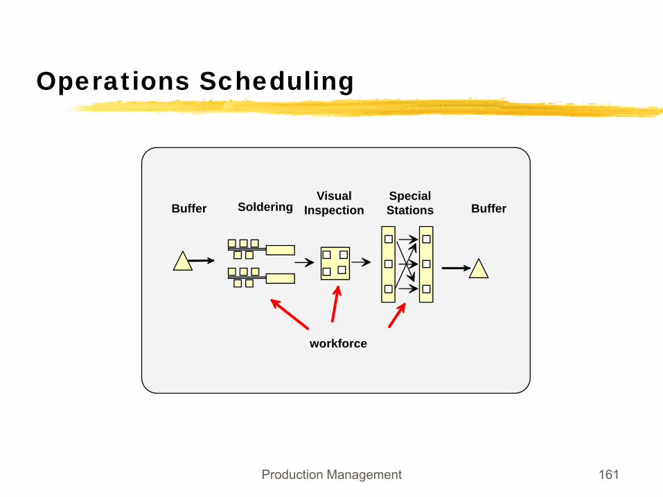
SolderingBuffer Buffer

workforce

VisualInspection

SpecialStations



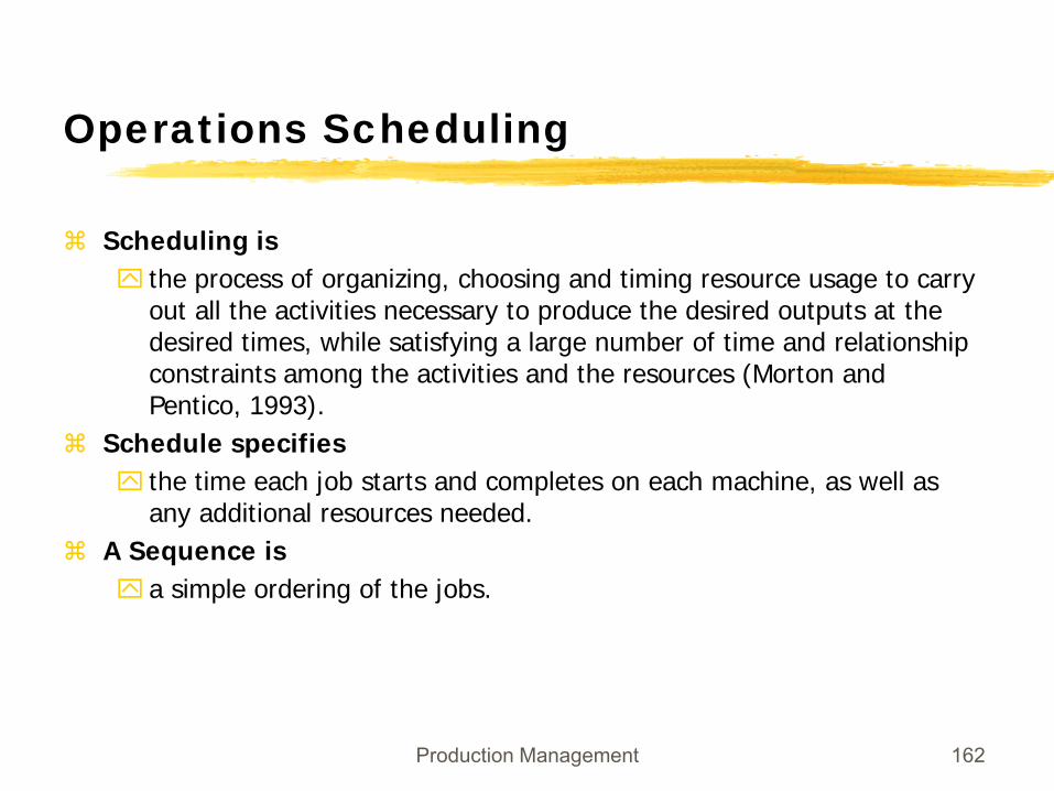
Scheduling is the process of organizing, choosing and timing resource usage to carry out all the activities necessary to produce the desired outputs at the desired times, while satisfying a large number of time and relationship constraints among the activities and the resources (Morton and Pentico, 1993).

Schedule specifiesthe time each job starts and completes on each machine, as well as any additional resources needed.

A Sequence isa simple ordering of the jobs.


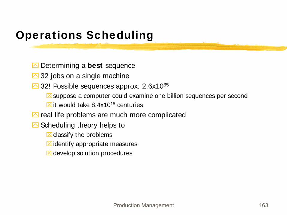
Determining a best sequence32 jobs on a single machine32! Possible sequences approx. 2.6x1035

⌧suppose a computer could examine one billion sequences per second⌧it would take 8.4x1015 centuries

real life problems are much more complicatedScheduling theory helps to ⌧classify the problems⌧identify appropriate measures⌧develop solution procedures



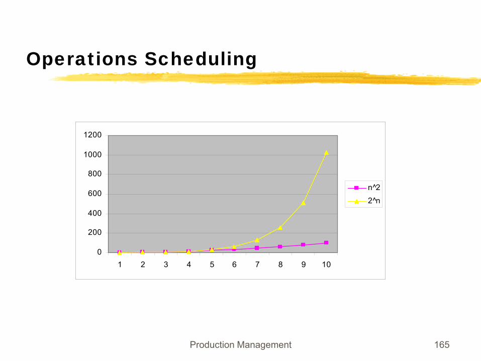
Algorithmic complexityan efficient algorithm is one whose effort of any problem instance is bounded by a polynomial in the problem size, e.g. # of jobsminimal spanning tree can be solved in at most n2 iterationsn: number of edgesO(n2)

if effort is exponential O(2n) the algorithm is not efficientbranch and bound algorithm for 0/1 variables

NP-hard problems: no exact algorithm in polynomial time is known. e.g. Traveling salesman problemHeuristics are usually polynomial algorithms tailored to the specific problem structure




0

200

400

600

800

1000

1200

1 2 3 4 5 6 7 8 9 10

n^2

2^n


Scheduling Theory (Background)Jobs are

activities to be doneprocessing time knownin general continously processed until finished (preemption not allowed)due date release dateprecedence constraintssequence dependent setup timeprocessed by at most one-machine at the same time



Machines (resources)single machine, parallel machinesflow shop: ⌧each job must be processed by each machine exactly once⌧all jobs have the same routing⌧a job cannot begin processing on the second machine until it has completed

processing on the first⌧assembly line

job shop:⌧each job may have a unique routing

open shops:⌧job shops in which jobs have no specific routing⌧re-manufacturing and repair



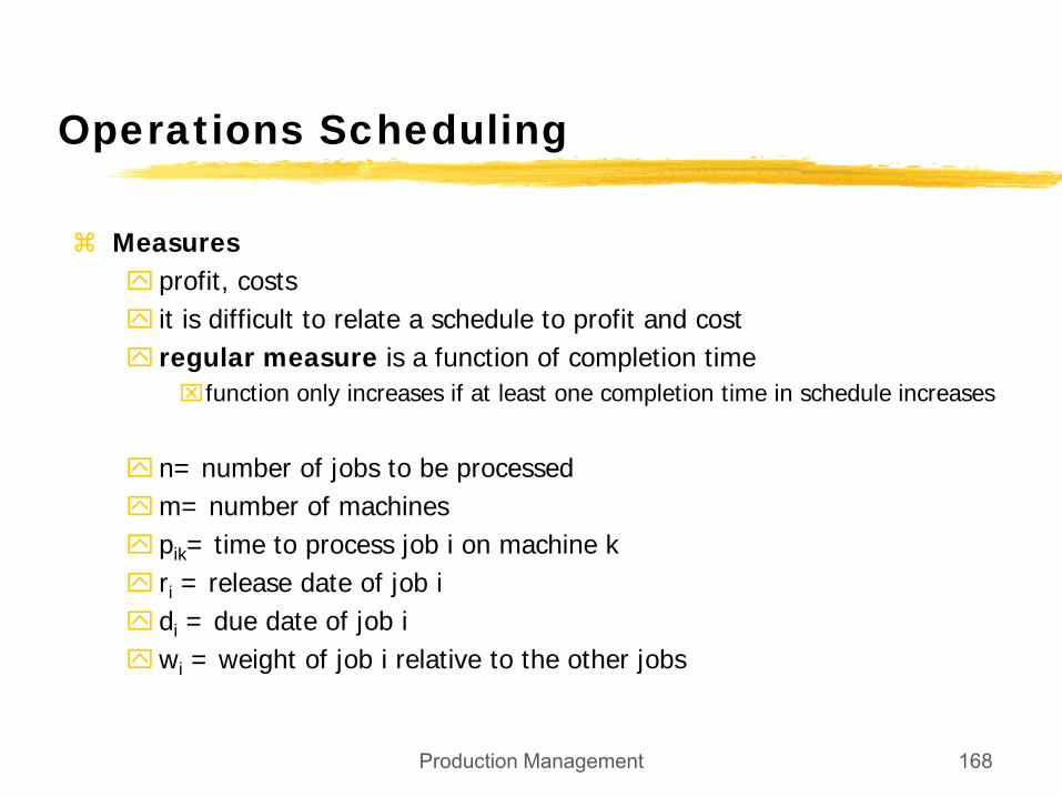
Measuresprofit, costsit is difficult to relate a schedule to profit and costregular measure is a function of completion time⌧function only increases if at least one completion time in schedule increases

n= number of jobs to be processedm= number of machinespik= time to process job i on machine kri = release date of job idi = due date of job iwi = weight of job i relative to the other jobs



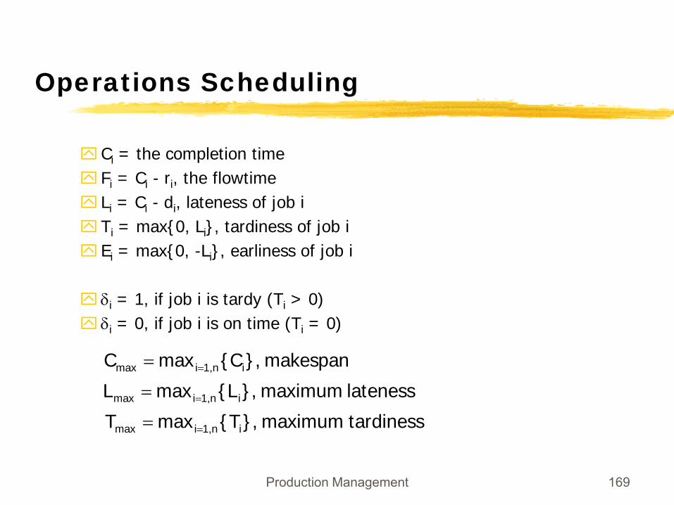
Ci = the completion timeFi = Ci - ri, the flowtimeLi = Ci - di, lateness of job iTi = max{0, Li}, tardiness of job iEi = max{0, -Li}, earliness of job i

δi = 1, if job i is tardy (Ti > 0)δi = 0, if job i is on time (Ti = 0)


tardiness maximum },{Tmax T

lateness maximum },{Lmax L

makespan},{Cmax C

in1,imax

in1,imax

in1,imax

=

=

=

=

=

=



Common proxy objectivestotal flowtimetotal tardinessmakespanmaximum tardinessnumber of tardy jobsif not all jobs are equally important weights should be introduced

minimizing total completion time is equivalent to minimizing total flowtime or minimizing total tardiness



Algorithms:exact algorithms often based on (worst case scenario) enumeration (e.g. Branch and Bound, Dynamic Programming)

heuristic algorithm judged by quality (difference to the optimal solution) and efficacy (computational effort)worst-case bounds are desirable to motivate use of a certain heuristic



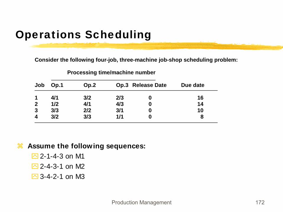
Assume the following sequences:2-1-4-3 on M12-4-3-1 on M23-4-2-1 on M3

Consider the following four-job, three-machine job-shop scheduling problem:

Processing time/machine number

Job Op.1 Op.2 Op.3 Release Date Due date

1 4/1 3/2 2/3 0 162 1/2 4/1 4/3 0 143 3/3 2/2 3/1 0 104 3/2 3/3 1/1 0 8



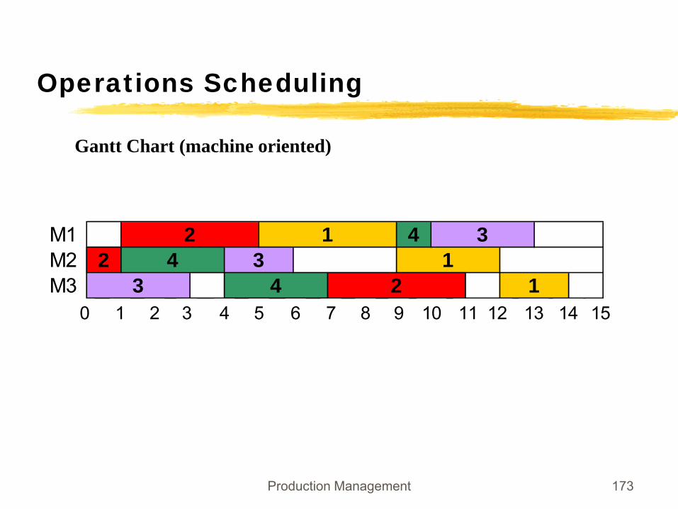
Gantt Chart (machine oriented)

M1 4M2 2M3 2

11

133

34

4

2

0 1 2 3 4 5 6 7 8 9 10 11 12 13 14 15



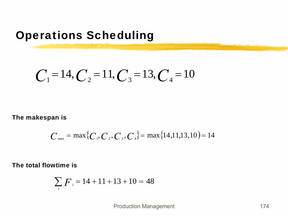
The makespan is

The total flowtime is

{ } ){ 1410,13,11,14max,,,max 4321max === CCCCC

4810131114 =+++=∑i

iF

10,13,11,144321==== CCCC



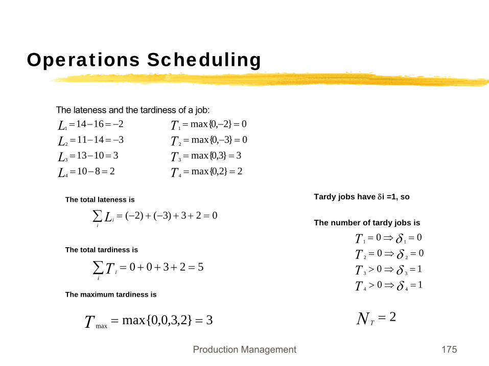
The lateness and the tardiness of a job:

281031013

3141121614

4

3

2

1

=−=

=−=

−=−=

−=−=

LLLL

2}2,0max{3}3,0max{

0}3,0max{0}2,0max{

4

3

2

1

==

==

=−=

=−=

TTTT

The total lateness is

The total tardiness is

The maximum tardiness is

023)3()2( =++−+−=∑i

iL

∑ =+++=i

iT 52300

3}2,3,0,0max{max ==T

Tardy jobs have δi =1, so

The number of tardy jobs is

10100000

44

33

22

11

=⇒>

=⇒>

=⇒=

=⇒=

δδδδ

TTTT

2=N T



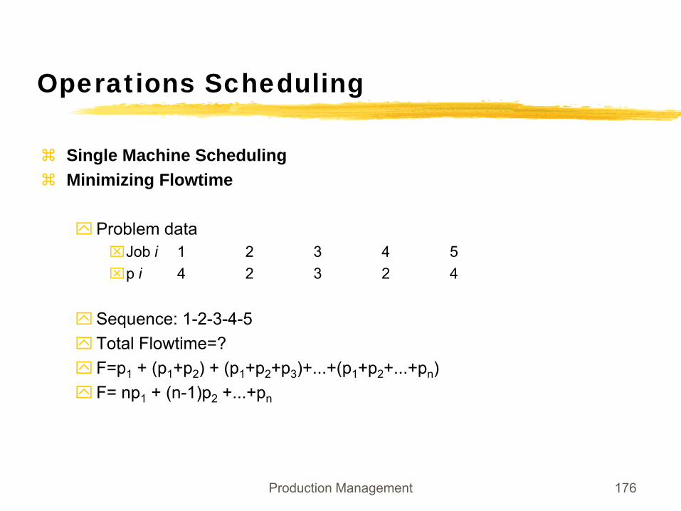
Single Machine SchedulingMinimizing Flowtime

Problem data⌧Job i 1 2 3 4 5⌧p i 4 2 3 2 4

Sequence: 1-2-3-4-5Total Flowtime=?F=p1 + (p1+p2) + (p1+p2+p3)+...+(p1+p2+...+pn)F= np1 + (n-1)p2 +...+pn



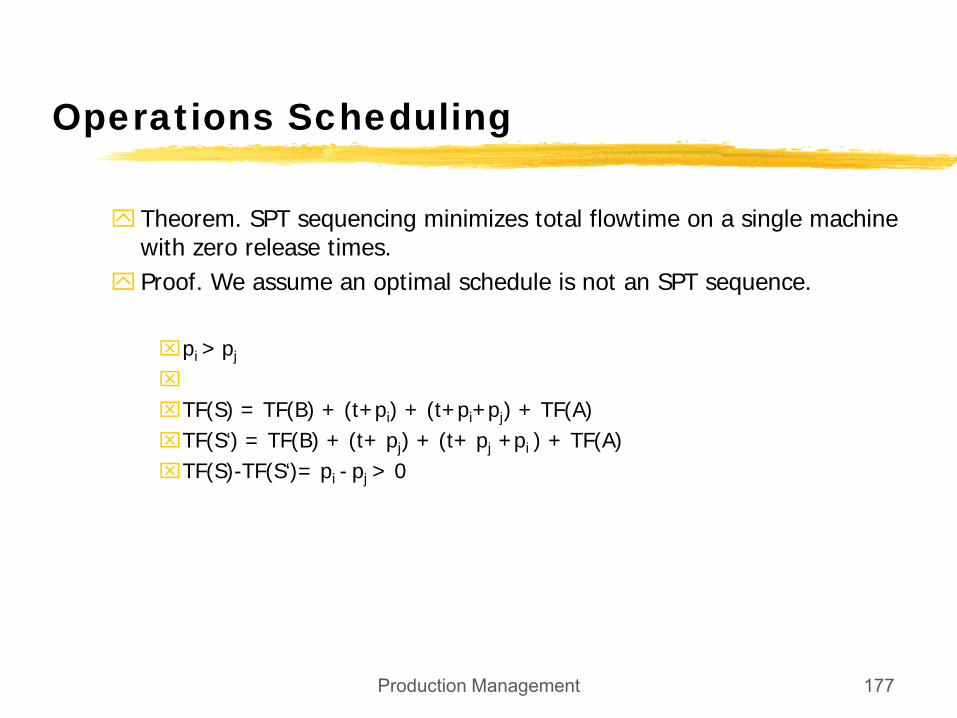
Theorem. SPT sequencing minimizes total flowtime on a single machine with zero release times.Proof. We assume an optimal schedule is not an SPT sequence.

⌧pi > pj

⌧

⌧TF(S) = TF(B) + (t+pi) + (t+pi+pj) + TF(A)⌧TF(S‘) = TF(B) + (t+ pj) + (t+ pj +pi ) + TF(A)⌧TF(S)-TF(S‘)= pi - pj > 0


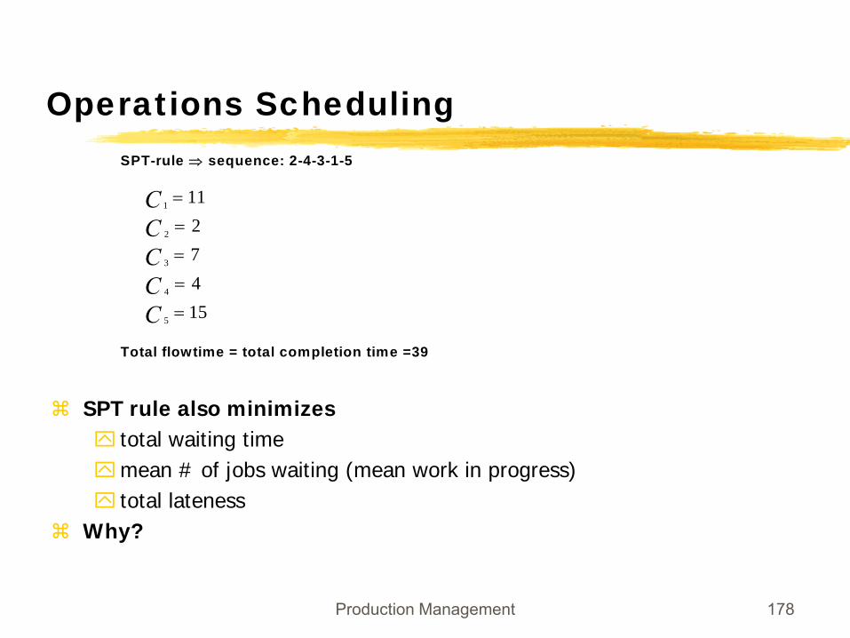
SPT-rule ⇒ sequence: 2-4-3-1-5

Total flowtime = total completion time =39

1547211

5

4

3

2

1

=

=

=

=

=

CCCCC


SPT rule also minimizestotal waiting time mean # of jobs waiting (mean work in progress)total lateness

Why?



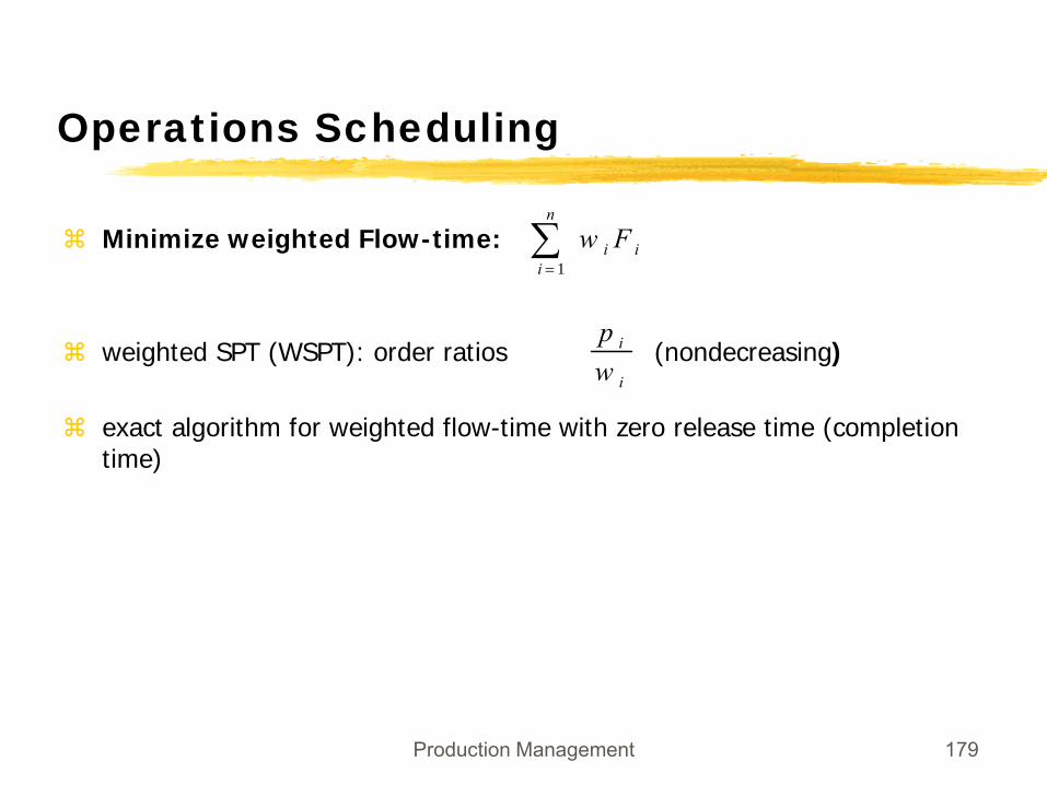
Minimize weighted Flow-time:

weighted SPT (WSPT): order ratios (nondecreasing)

exact algorithm for weighted flow-time with zero release time (completion time)

∑=

n

iii Fw

1

i

i

wp


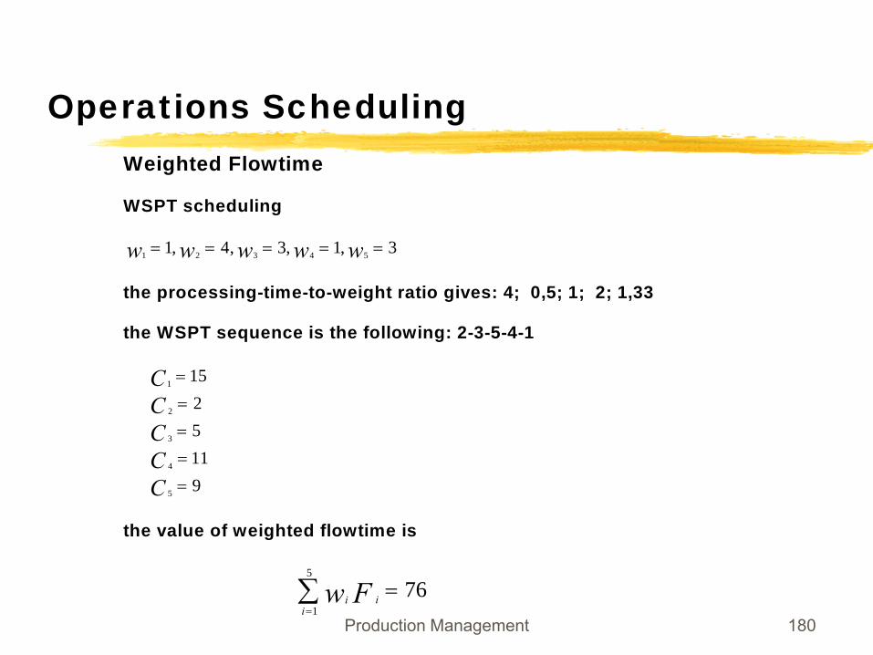
Operations SchedulingWeighted Flowtime

WSPT scheduling

the processing-time-to-weight ratio gives: 4; 0,5; 1; 2; 1,33

the WSPT sequence is the following: 2-3-5-4-1

the value of weighted flowtime is

3,1,3,4,1 54321 ===== wwwww

9115215

5

4

3

2

1

=

=

=

=

=

CCCCC

∑=

=5

176

iii Fw



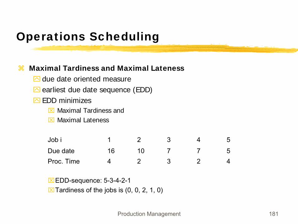
Maximal Tardiness and Maximal Latenessdue date oriented measureearliest due date sequence (EDD)EDD minimizes ⌧ Maximal Tardiness and ⌧ Maximal Lateness

Job i 1 2 3 4 5

Due date 16 10 7 7 5Proc. Time 4 2 3 2 4

⌧EDD-sequence: 5-3-4-2-1⌧Tardiness of the jobs is (0, 0, 2, 1, 0)



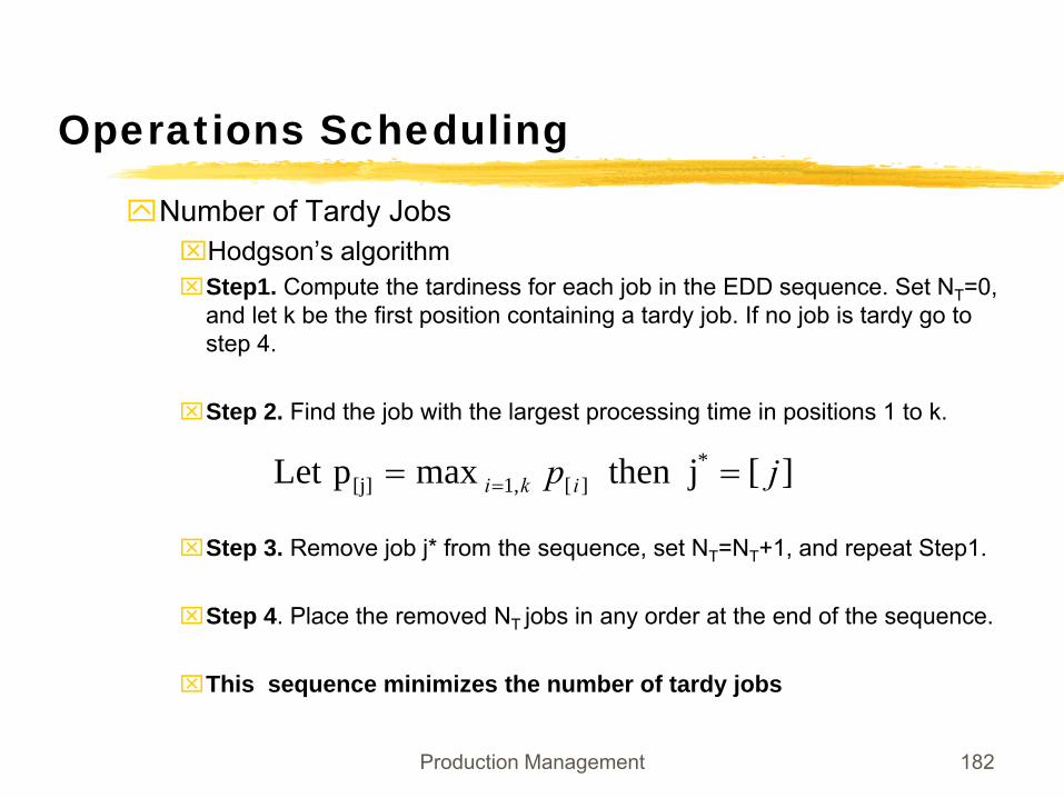
Number of Tardy Jobs⌧Hodgson’s algorithm⌧Step1. Compute the tardiness for each job in the EDD sequence. Set NT=0,

and let k be the first position containing a tardy job. If no job is tardy go to step 4.

⌧Step 2. Find the job with the largest processing time in positions 1 to k.

⌧Step 3. Remove job j* from the sequence, set NT=NT+1, and repeat Step1.

⌧Step 4. Place the removed NT jobs in any order at the end of the sequence.

⌧This sequence minimizes the number of tardy jobs

][j then maxpLet *][,1[j] jp iki == =


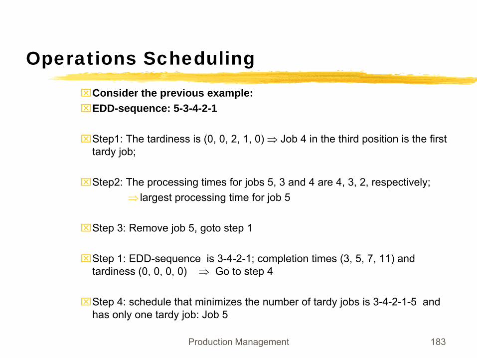
Operations Scheduling⌧Consider the previous example:⌧EDD-sequence: 5-3-4-2-1

⌧Step1: The tardiness is (0, 0, 2, 1, 0) ⇒ Job 4 in the third position is the first tardy job;

⌧Step2: The processing times for jobs 5, 3 and 4 are 4, 3, 2, respectively;⇒ largest processing time for job 5

⌧Step 3: Remove job 5, goto step 1

⌧Step 1: EDD-sequence is 3-4-2-1; completion times (3, 5, 7, 11) and tardiness (0, 0, 0, 0) ⇒ Go to step 4

⌧Step 4: schedule that minimizes the number of tardy jobs is 3-4-2-1-5 and has only one tardy job: Job 5



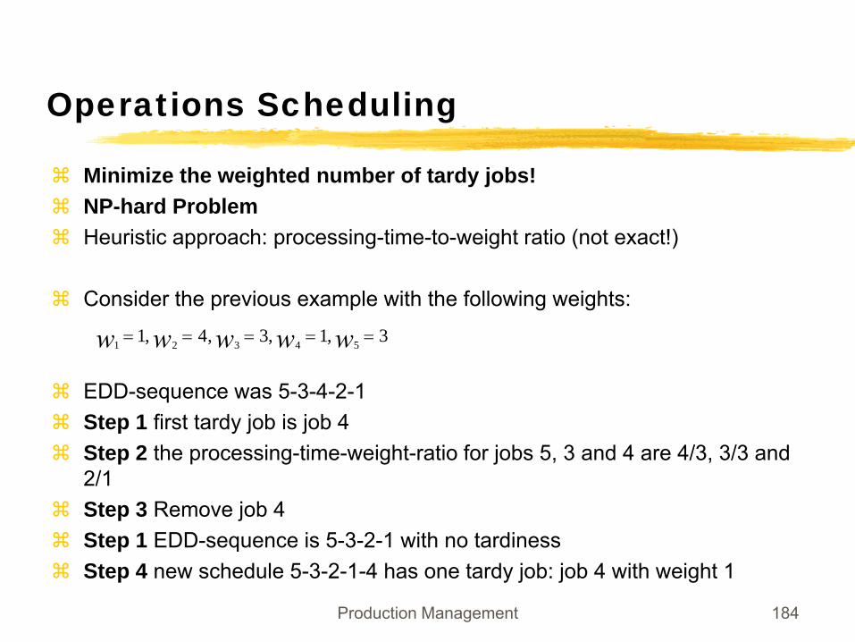
Minimize the weighted number of tardy jobs!NP-hard ProblemHeuristic approach: processing-time-to-weight ratio (not exact!)

Consider the previous example with the following weights:

EDD-sequence was 5-3-4-2-1Step 1 first tardy job is job 4Step 2 the processing-time-weight-ratio for jobs 5, 3 and 4 are 4/3, 3/3 and 2/1Step 3 Remove job 4Step 1 EDD-sequence is 5-3-2-1 with no tardinessStep 4 new schedule 5-3-2-1-4 has one tardy job: job 4 with weight 1

3,1,3,4,1 54321 ===== wwwww



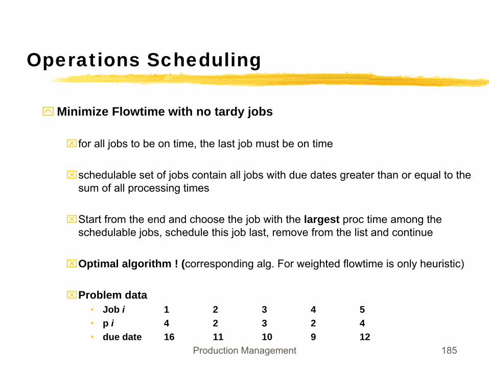
Minimize Flowtime with no tardy jobs

⌧for all jobs to be on time, the last job must be on time

⌧schedulable set of jobs contain all jobs with due dates greater than or equal to the sum of all processing times

⌧Start from the end and choose the job with the largest proc time among the schedulable jobs, schedule this job last, remove from the list and continue

⌧Optimal algorithm ! (corresponding alg. For weighted flowtime is only heuristic)

⌧Problem data• Job i 1 2 3 4 5• p i 4 2 3 2 4• due date 16 11 10 9 12



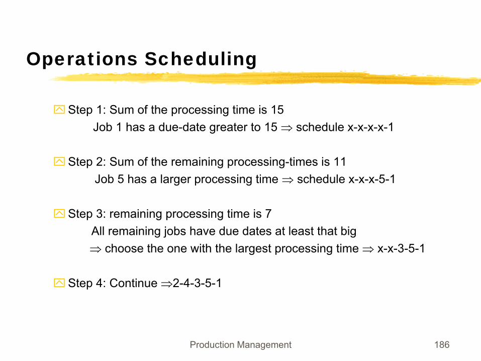
Step 1: Sum of the processing time is 15 Job 1 has a due-date greater to 15 ⇒ schedule x-x-x-x-1

Step 2: Sum of the remaining processing-times is 11Job 5 has a larger processing time ⇒ schedule x-x-x-5-1

Step 3: remaining processing time is 7All remaining jobs have due dates at least that big⇒ choose the one with the largest processing time ⇒ x-x-3-5-1

Step 4: Continue ⇒2-4-3-5-1



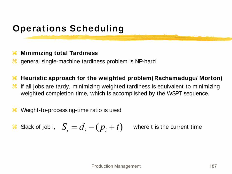
Minimizing total Tardinessgeneral single-machine tardiness problem is NP-hard

Heuristic approach for the weighted problem(Rachamadugu/Morton)if all jobs are tardy, minimizing weighted tardiness is equivalent to minimizing weighted completion time, which is accomplished by the WSPT sequence.

Weight-to-processing-time ratio is used

Slack of job i, where t is the current time)( tpdS iii +−=



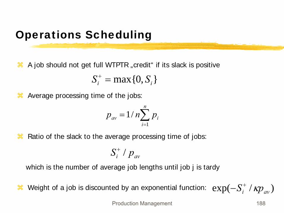
A job should not get full WTPTR „credit“ if its slack is positive

Average processing time of the jobs:

Ratio of the slack to the average processing time of jobs:

which is the number of average job lengths until job j is tardy

Weight of a job is discounted by an exponential function:

},0max{ ii SS =+

∑=

=n

iiav pnp

1/1

avi pS /+

)/exp( avi pS κ+−



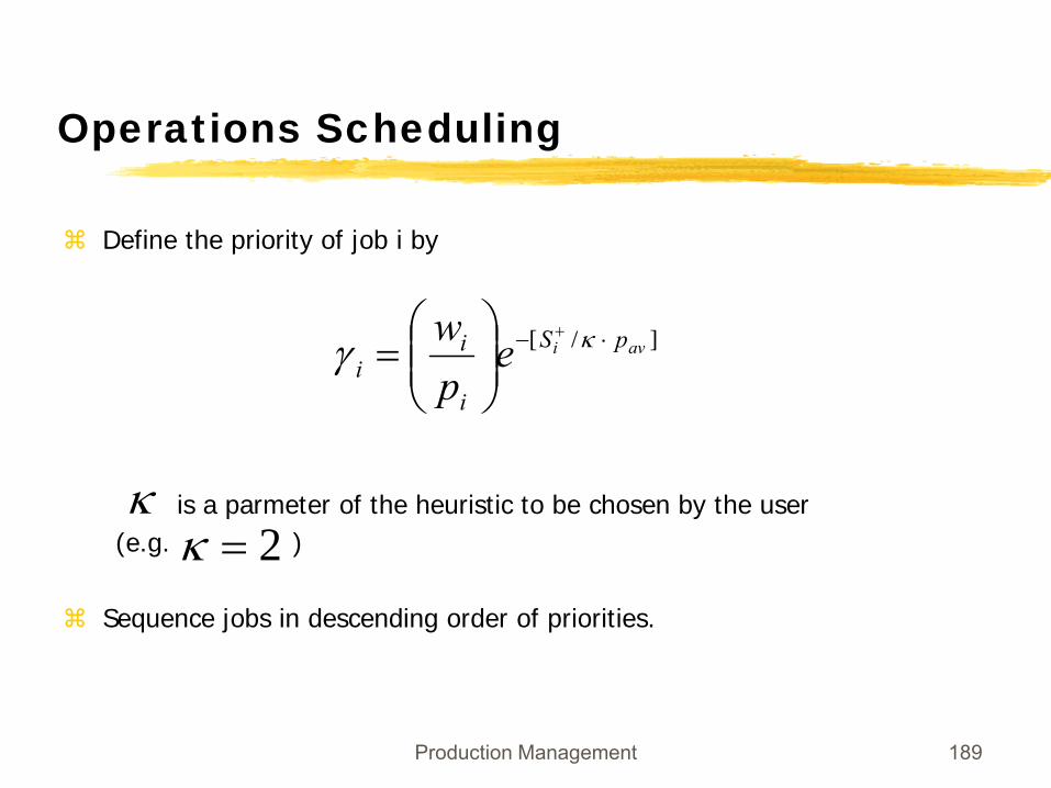
Define the priority of job i by

is a parmeter of the heuristic to be chosen by the user (e.g. )

Sequence jobs in descending order of priorities.

]/[ avi pS

i

ii e

pw ⋅− +

⎟⎟⎠

⎞⎜⎜⎝

⎛= κγ

κ2=κ



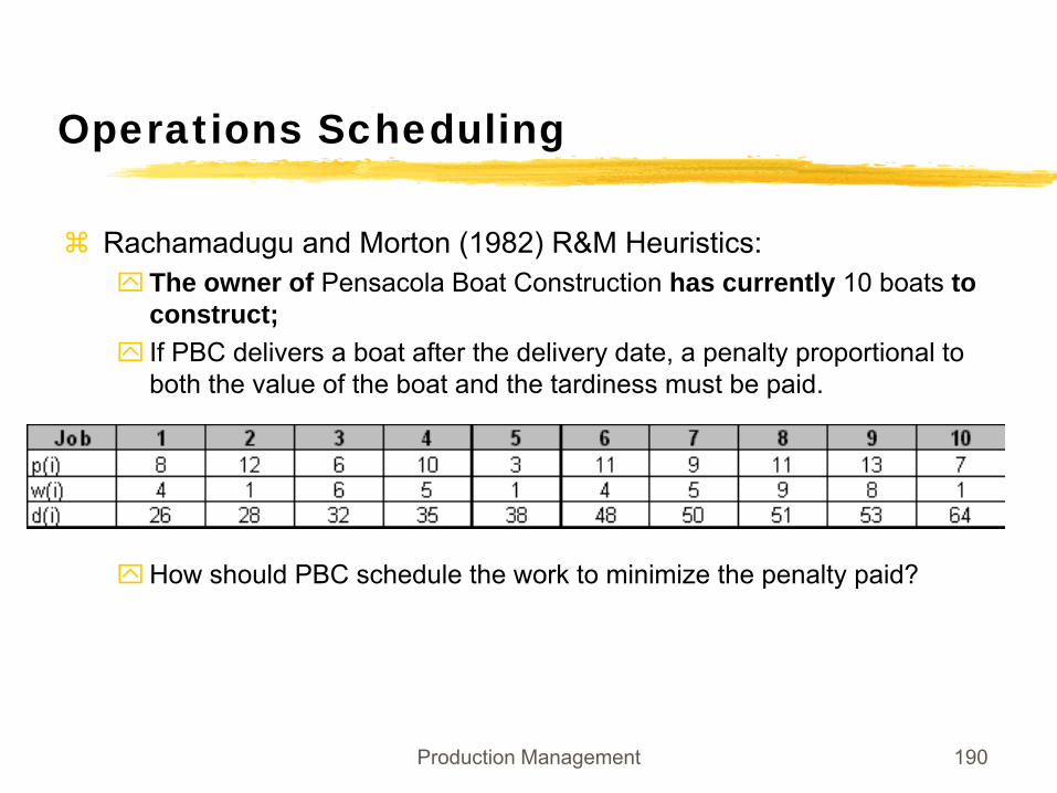
Rachamadugu and Morton (1982) R&M Heuristics:The owner of Pensacola Boat Construction has currently 10 boats to construct;If PBC delivers a boat after the delivery date, a penalty proportional to both the value of the boat and the tardiness must be paid.

How should PBC schedule the work to minimize the penalty paid?



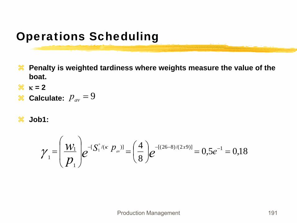
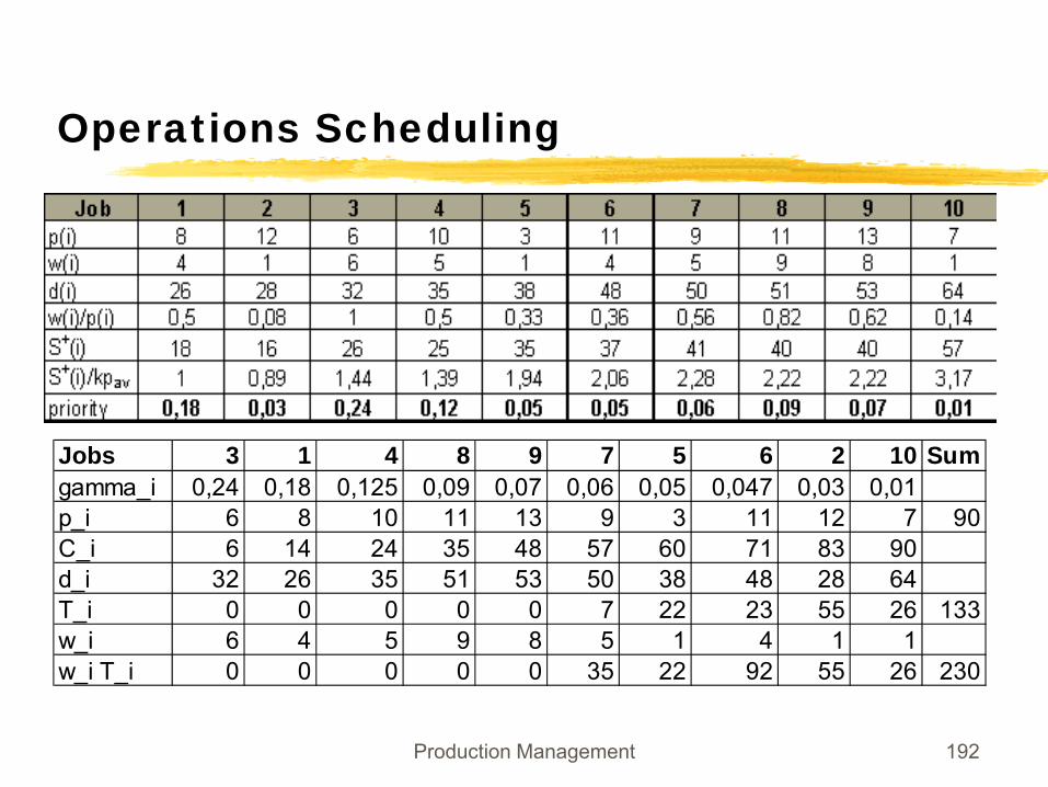
Penalty is weighted tardiness where weights measure the value of the boat.κ = 2Calculate:

Job1:

18,05,084 1)]92/()826[()]/([

1

11

1 ==⎟⎠⎞

⎜⎝⎛=⎟

⎟

⎠

⎞

⎜⎜

⎝

⎛= −−−−

+

epS eepw x

avκγ

9=avp



Jobs 3 1 4 8 9 7 5 6 2 10 Sumgamma_i 0,24 0,18 0,125 0,09 0,07 0,06 0,05 0,047 0,03 0,01p_i 6 8 10 11 13 9 3 11 12 7 90C_i 6 14 24 35 48 57 60 71 83 90d_i 32 26 35 51 53 50 38 48 28 64T_i 0 0 0 0 0 7 22 23 55 26 133w_i 6 4 5 9 8 5 1 4 1 1w_i T_i 0 0 0 0 0 35 22 92 55 26 230



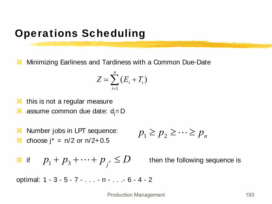
Minimizing Earliness and Tardiness with a Common Due-Date

this is not a regular measureassume common due date: dj=D

Number jobs in LPT sequence: choose j* = n/2 or n/2+0.5

if then the following sequence is

optimal: 1 - 3 - 5 - 7 - . . . - n - . . .- 6 - 4 - 2

∑=

+=n

iii TEZ

1)(

nppp ≥≥≥ L21

Dpppj≤+++ *31 L



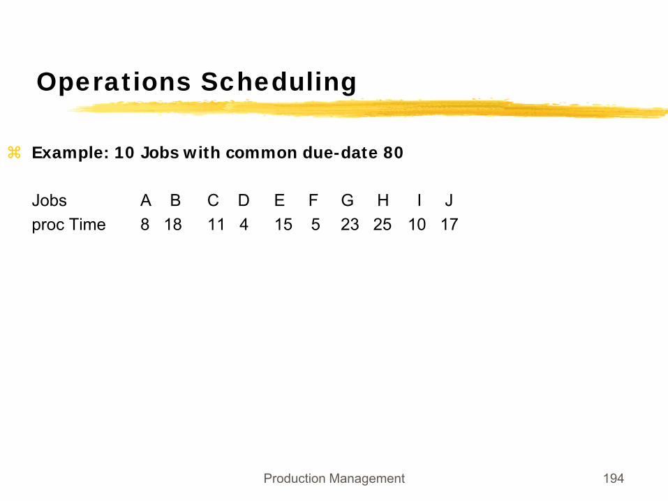
Example: 10 Jobs with common due-date 80

Jobs A B C D E F G H I Jproc Time 8 18 11 4 15 5 23 25 10 17



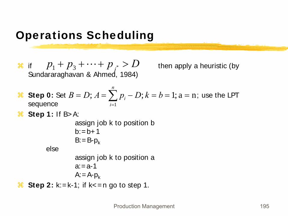
if then apply a heuristic (by Sundararaghavan & Ahmed, 1984)

Step 0: Set ; use the LPT sequenceStep 1: If B>A:

assign job k to position bb:=b+1B:=B-pk

elseassign job k to position aa:=a-1A:=A-pk

Step 2: k:=k-1; if k<=n go to step 1.

na ;1 ; ;1

===−== ∑=

n

ii bkDpADB

Dpppj>+++ *31 L



Problems with non-zero release time

Non-zero release times typically makes scheduling problems much harder, e.g. SPT does in general not minimize total flowtime

Heuristic Approach:At each time t determine the set of schedulable jobs: jobs that have been released but not yet processed.

Choose from the schedulable jobs according to some rule (e.g. SPT for minimizing flowtime)



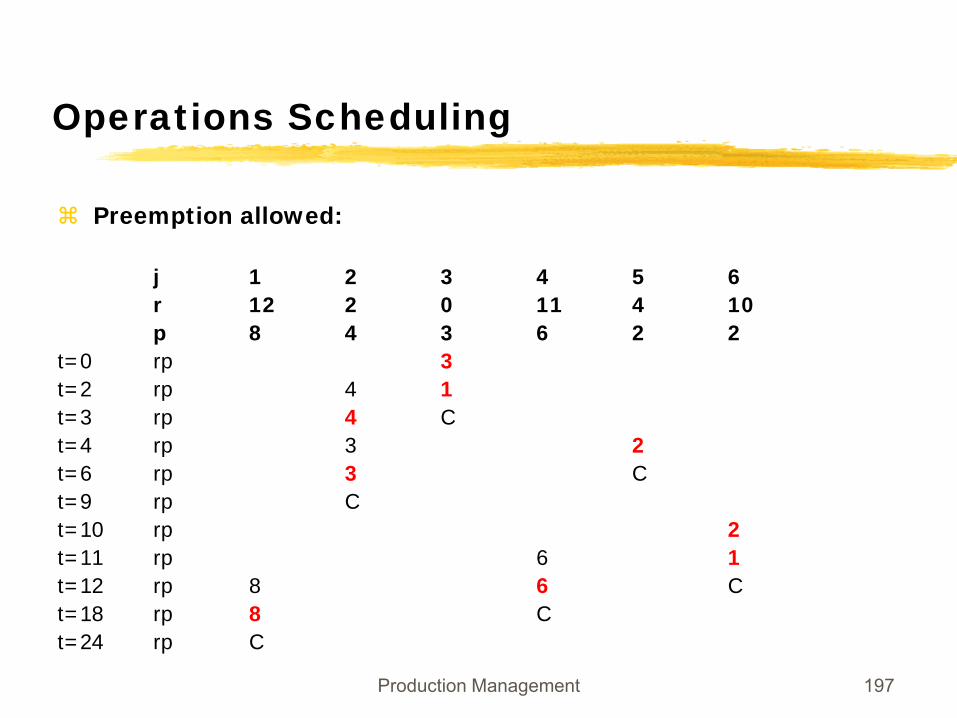
Preemption allowed:

j 1 2 3 4 5 6r 12 2 0 11 4 10p 8 4 3 6 2 2

t=0 rp 3t=2 rp 4 1t=3 rp 4 Ct=4 rp 3 2t=6 rp 3 Ct=9 rp Ct=10 rp 2t=11 rp 6 1t=12 rp 8 6 Ct=18 rp 8 Ct=24 rp C



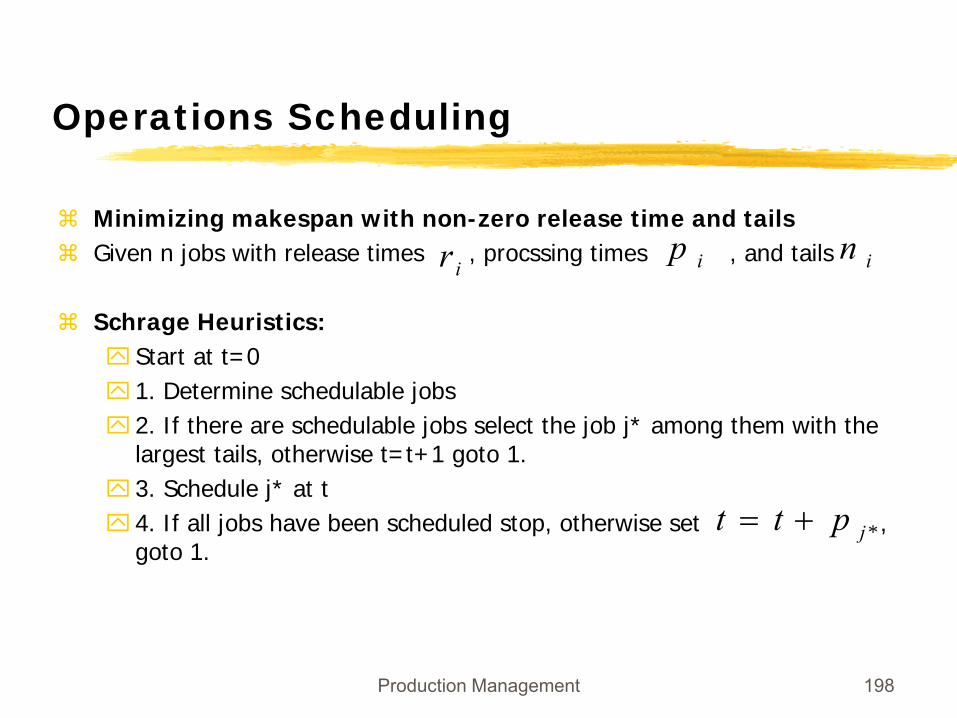
Minimizing makespan with non-zero release time and tailsGiven n jobs with release times , procssing times , and tails

Schrage Heuristics:Start at t=01. Determine schedulable jobs2. If there are schedulable jobs select the job j* among them with the largest tails, otherwise t=t+1 goto 1.3. Schedule j* at t4. If all jobs have been scheduled stop, otherwise set , goto 1.

ir ip in

*jptt +=



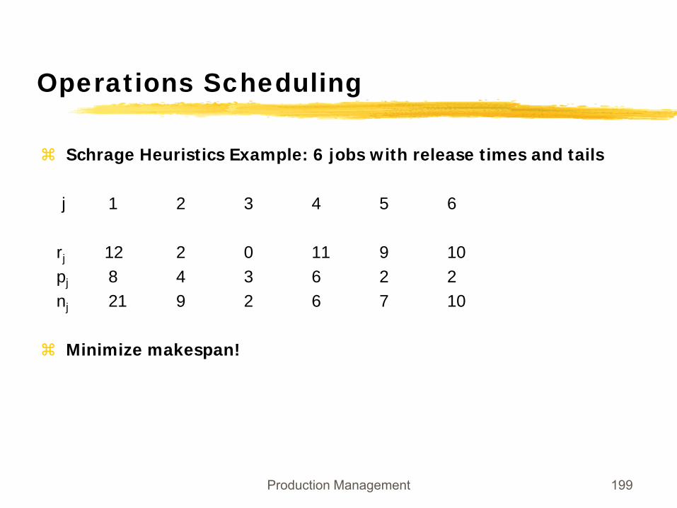
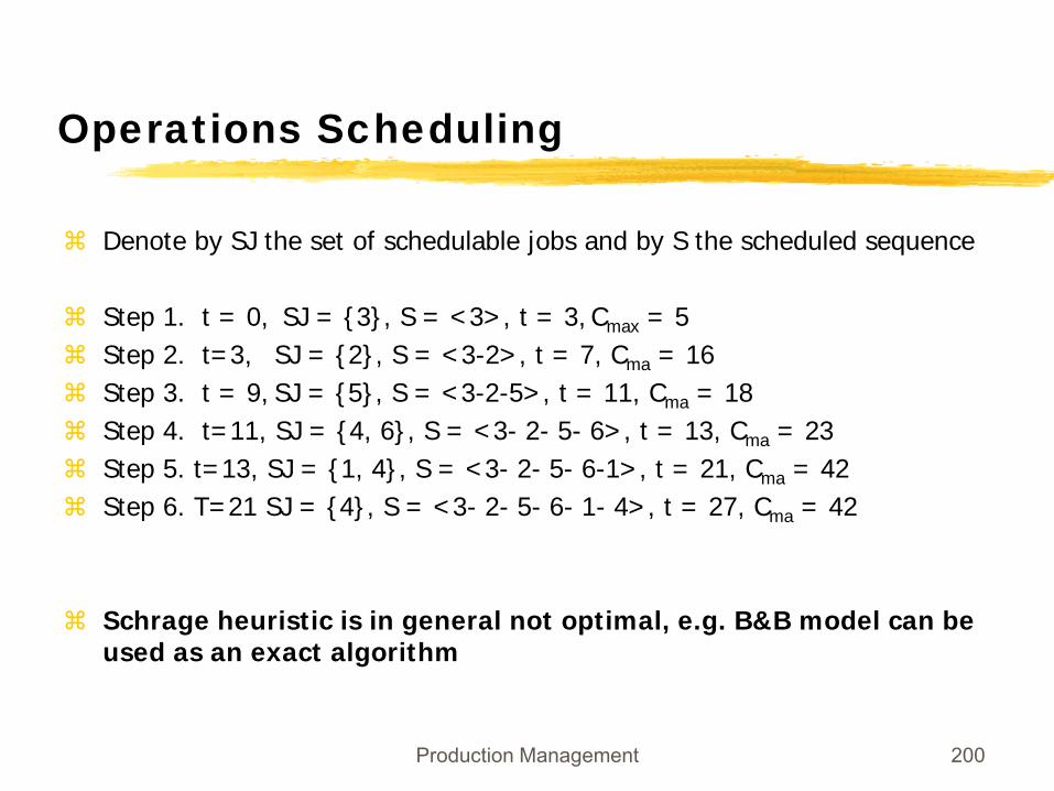
Schrage Heuristics Example: 6 jobs with release times and tails

j 1 2 3 4 5 6

rj 12 2 0 11 9 10pj 8 4 3 6 2 2nj 21 9 2 6 7 10

Minimize makespan!



Denote by SJ the set of schedulable jobs and by S the scheduled sequence

Step 1. t = 0, SJ = {3}, S = <3>, t = 3, Cmax = 5Step 2. t=3, SJ = {2}, S = <3-2>, t = 7, Cma = 16Step 3. t = 9, SJ = {5}, S = <3-2-5>, t = 11, Cma = 18Step 4. t=11, SJ = {4, 6}, S = <3- 2- 5- 6>, t = 13, Cma = 23Step 5. t=13, SJ = {1, 4}, S = <3- 2- 5- 6-1>, t = 21, Cma = 42Step 6. T=21 SJ = {4}, S = <3- 2- 5- 6- 1- 4>, t = 27, Cma = 42

Schrage heuristic is in general not optimal, e.g. B&B model can be used as an exact algorithm



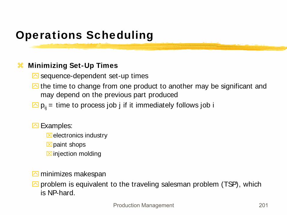
Minimizing Set-Up Timessequence-dependent set-up timesthe time to change from one product to another may be significant and may depend on the previous part producedpij = time to process job j if it immediately follows job i

Examples:⌧electronics industry⌧paint shops⌧injection molding

minimizes makespanproblem is equivalent to the traveling salesman problem (TSP), which is NP-hard.


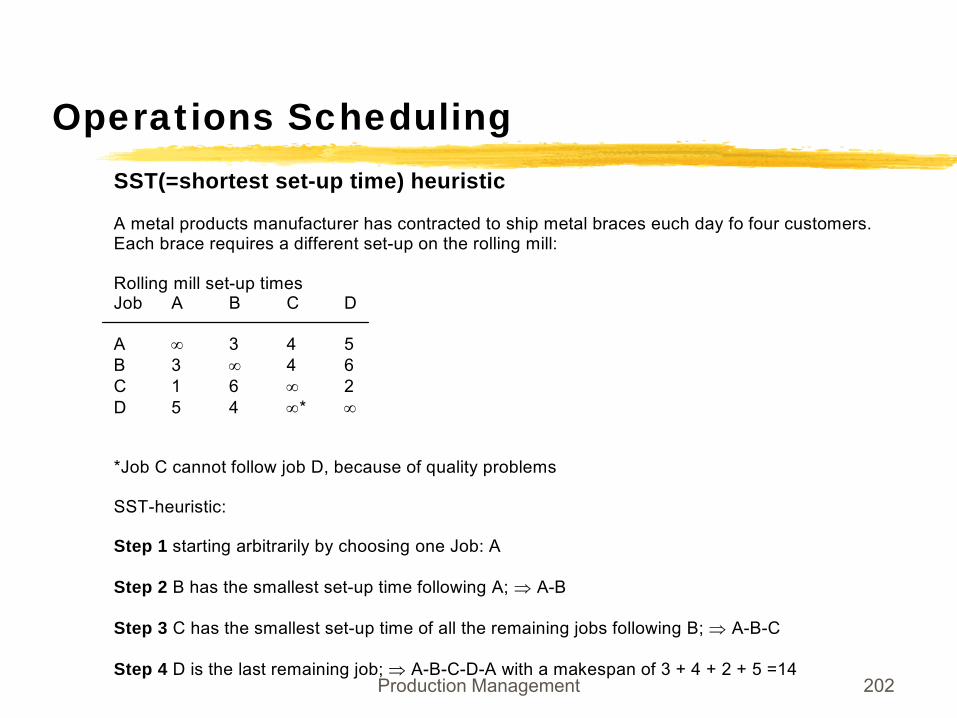
Operations SchedulingSST(=shortest set-up time) heuristic

A metal products manufacturer has contracted to ship metal braces euch day fo four customers.Each brace requires a different set-up on the rolling mill:

Rolling mill set-up timesJob A B C D

A ∞ 3 4 5B 3 ∞ 4 6C 1 6 ∞ 2D 5 4 ∞* ∞

*Job C cannot follow job D, because of quality problems

SST-heuristic:

Step 1 starting arbitrarily by choosing one Job: A

Step 2 B has the smallest set-up time following A; ⇒ A-B

Step 3 C has the smallest set-up time of all the remaining jobs following B; ⇒ A-B-C

Step 4 D is the last remaining job; ⇒ A-B-C-D-A with a makespan of 3 + 4 + 2 + 5 =14



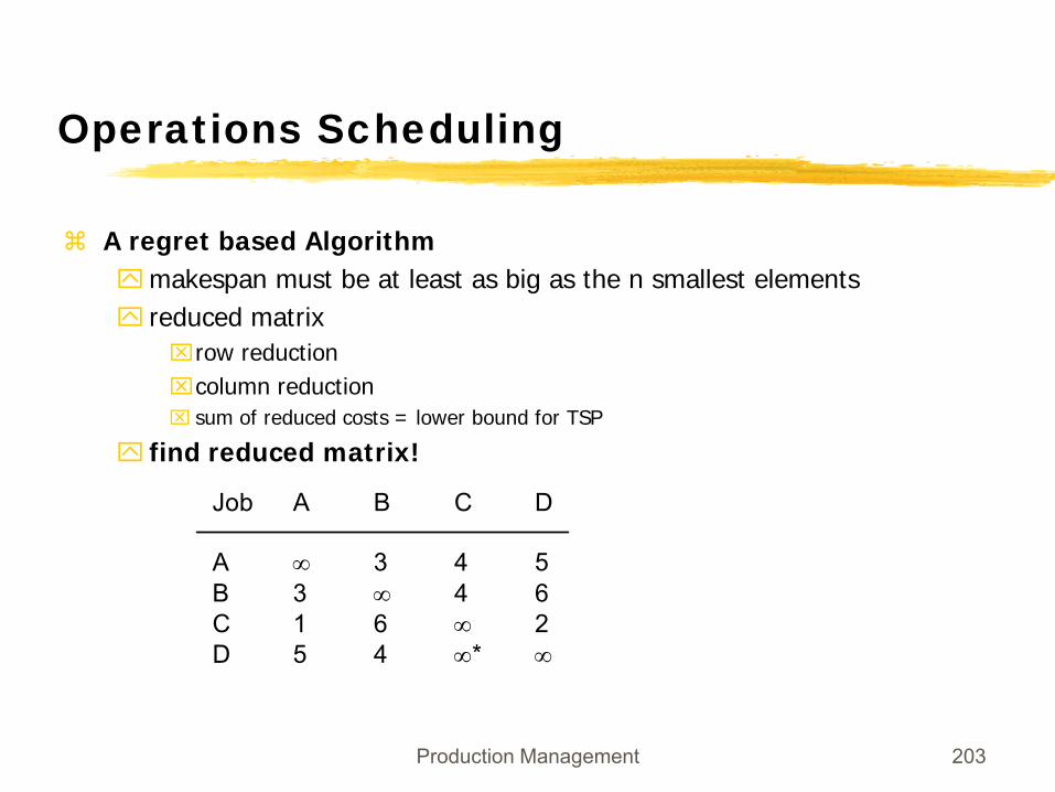
A regret based Algorithmmakespan must be at least as big as the n smallest elementsreduced matrix⌧row reduction⌧column reduction⌧ sum of reduced costs = lower bound for TSP

find reduced matrix!

Job A B C D

A ∞ 3 4 5B 3 ∞ 4 6C 1 6 ∞ 2D 5 4 ∞* ∞



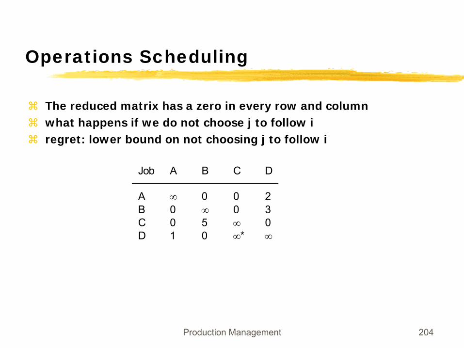
The reduced matrix has a zero in every row and columnwhat happens if we do not choose j to follow iregret: lower bound on not choosing j to follow i

Job A B C D

A ∞ 0 0 2B 0 ∞ 0 3C 0 5 ∞ 0D 1 0 ∞* ∞



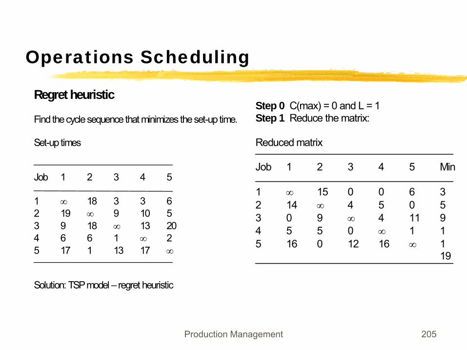
Regret heuristic

Find the cycle sequence that minimizes the set-up time.

Set-up times

Job 1 2 3 4 5

1 ∞ 18 3 3 62 19 ∞ 9 10 53 9 18 ∞ 13 204 6 6 1 ∞ 25 17 1 13 17 ∞

Solution: TSP model – regret heuristic

Step 0 C(max) = 0 and L = 1Step 1 Reduce the matrix:

Reduced matrix

Job 1 2 3 4 5 Min

1 ∞ 15 0 0 6 32 14 ∞ 4 5 0 53 0 9 ∞ 4 11 94 5 5 0 ∞ 1 15 16 0 12 16 ∞ 1

19



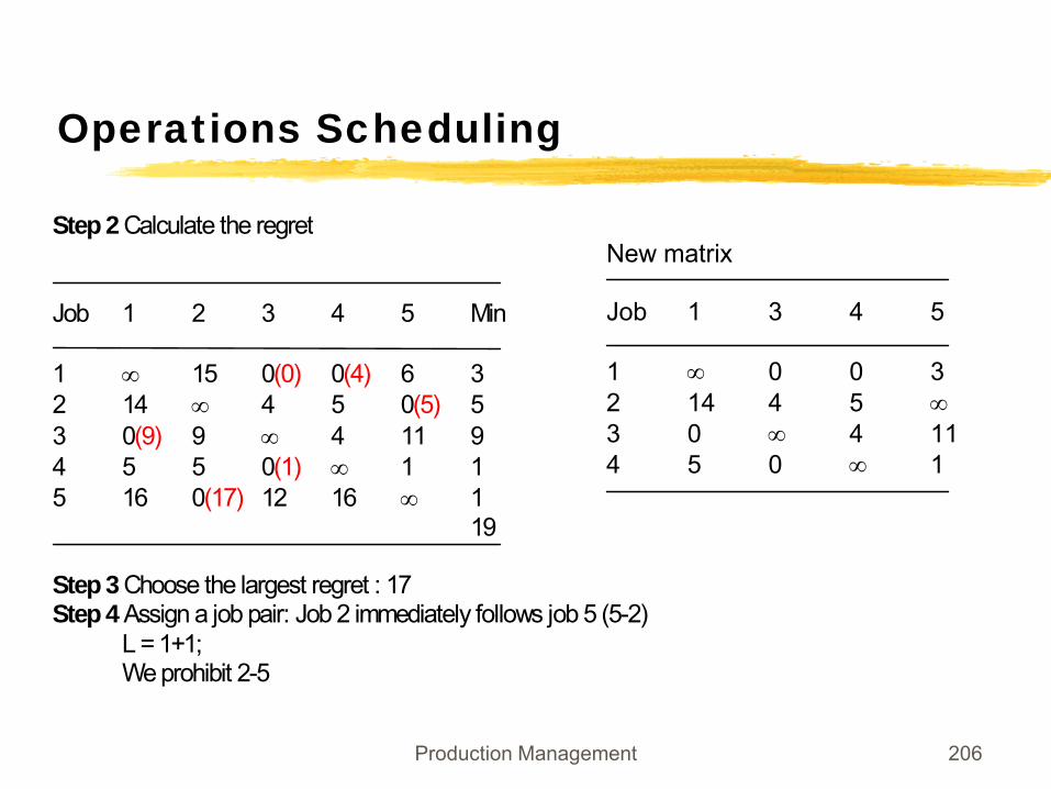
Step 2 Calculate the regret

Job 1 2 3 4 5 Min

1 ∞ 15 0(0) 0(4) 6 32 14 ∞ 4 5 0(5) 53 0(9) 9 ∞ 4 11 94 5 5 0(1) ∞ 1 15 16 0(17) 12 16 ∞ 1

19

Step 3 Choose the largest regret : 17Step 4 Assign a job pair: Job 2 immediately follows job 5 (5-2)

L = 1+1;We prohibit 2-5

New matrix

Job 1 3 4 5

1 ∞ 0 0 32 14 4 5 ∞3 0 ∞ 4 114 5 0 ∞ 1


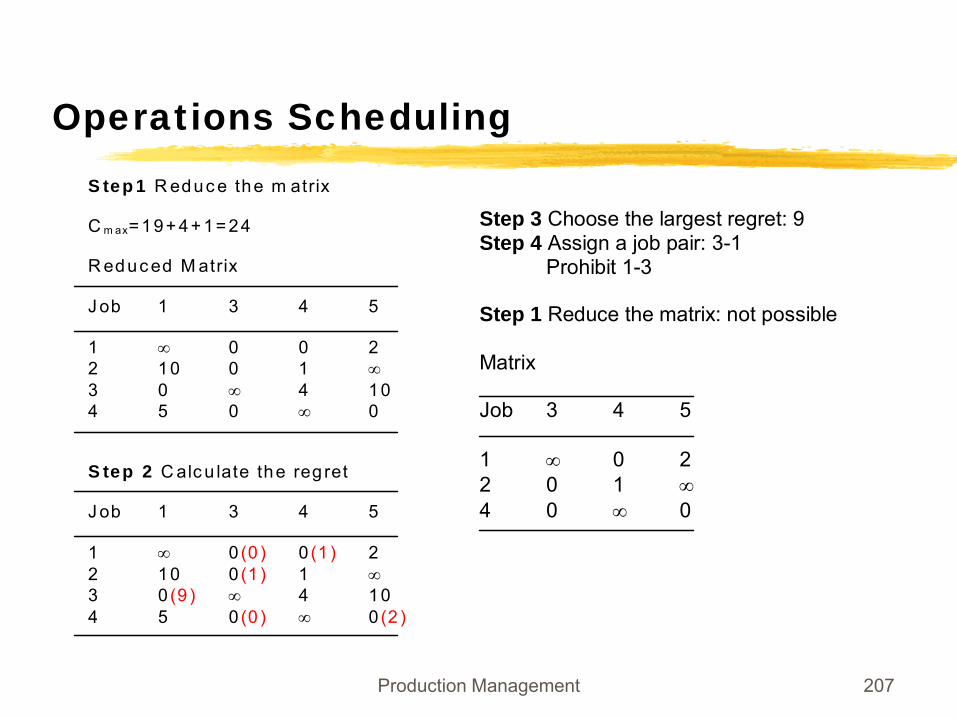
Operations SchedulingS tep 1 R educ e the m atrix C m ax= 19+ 4+ 1= 24 R educ ed M atrix J ob 1 3 4 5 1 ∞ 0 0 2 2 10 0 1 ∞ 3 0 ∞ 4 10 4 5 0 ∞ 0 S tep 2 C alc u late the reg ret J ob 1 3 4 5 1 ∞ 0 (0 ) 0 (1 ) 2 2 10 0 (1 ) 1 ∞ 3 0 (9 ) ∞ 4 10 4 5 0 (0 ) ∞ 0 (2 )

Step 3 Choose the largest regret: 9Step 4 Assign a job pair: 3-1

Prohibit 1-3

Step 1 Reduce the matrix: not possible

Matrix

Job 3 4 5

1 ∞ 0 22 0 1 ∞4 0 ∞ 0



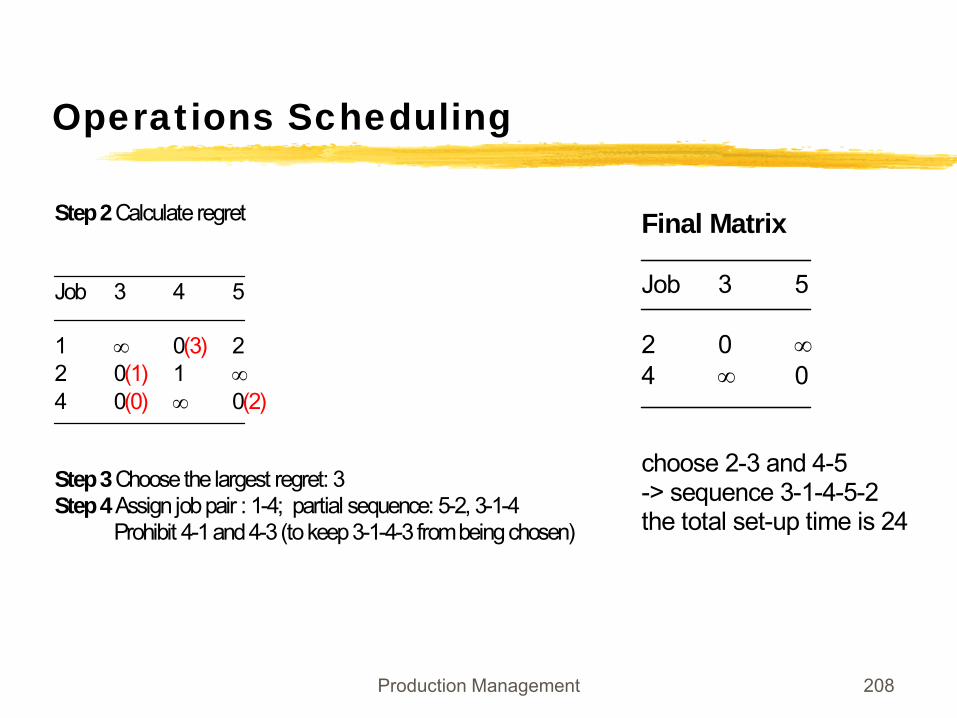
Step 2Calculate regret

Job 3 4 5

1 ∞ 0(3) 22 0(1) 1 ∞4 0(0) ∞ 0(2)

Step 3 Choose the largest regret: 3Step 4 Assign job pair : 1-4; partial sequence: 5-2, 3-1-4

Prohibit 4-1 and 4-3 (to keep 3-1-4-3 from being chosen)

Final Matrix

Job 3 5

2 0 ∞4 ∞ 0

choose 2-3 and 4-5-> sequence 3-1-4-5-2the total set-up time is 24



Branch and Bound Algorithm1. Using the regret heuristic construct a (sub-)tree where each node represents the decision to let j follow i ( ) or to prohibit that j follows i ( )2. For each node a lower bound for the makespan is inferred from the regret heuristic3. Once a solution is obtained from the regret heuristic this is an upper bound for the optimal makespan. All nodes where the lower bound is above that level are pruned.4. If all but one final node are pruned (or no non-pruned node can be further branched) this final node gives the optimal solution. 5. If 4. does not hold start again with 1. at one of nodes which are not pruned and can still be branched.

ji −ji −



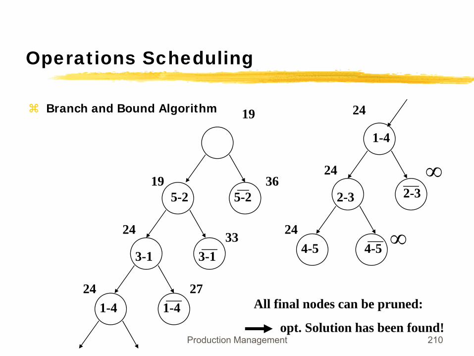
Branch and Bound Algorithm

5-2 5-2

3-13-1

1-4 1-4

19

24

24

36

33

27

19

1-4

2-3

4-5 4-5

24

24

2-3

24

∞

∞

All final nodes can be pruned:

opt. Solution has been found!



Single-Machine Search MethodsNeighborhood SearchSimulated AnnealingAnt SystemTabu Search...

Neighborhood SearchseedNeighborhoodany heuristic can be used to produce an initial sequence



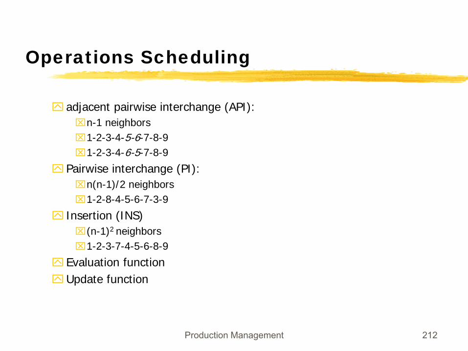
adjacent pairwise interchange (API):⌧n-1 neighbors⌧1-2-3-4-5-6-7-8-9⌧1-2-3-4-6-5-7-8-9

Pairwise interchange (PI):⌧n(n-1)/2 neighbors⌧1-2-8-4-5-6-7-3-9

Insertion (INS)⌧(n-1)2 neighbors⌧1-2-3-7-4-5-6-8-9

Evaluation functionUpdate function


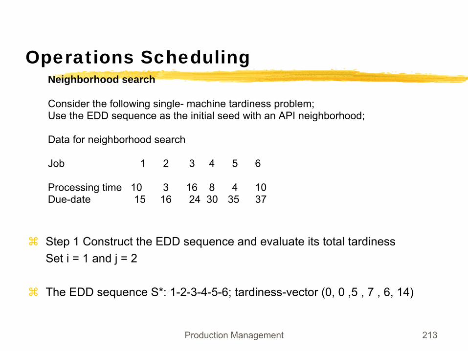
Operations SchedulingNeighborhood search

Consider the following single- machine tardiness problem;Use the EDD sequence as the initial seed with an API neighborhood;

Data for neighborhood search

Job 1 2 3 4 5 6

Processing time 10 3 16 8 4 10Due-date 15 16 24 30 35 37

Step 1 Construct the EDD sequence and evaluate its total tardinessSet i = 1 and j = 2

The EDD sequence S*: 1-2-3-4-5-6; tardiness-vector (0, 0 ,5 , 7 , 6, 14)



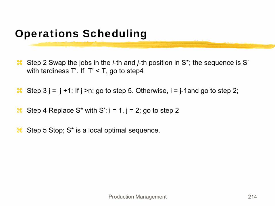
Step 2 Swap the jobs in the i-th and j-th position in S*; the sequence is S’ with tardiness T’. If T’ < T, go to step4

Step 3 j = j +1: If j >n: go to step 5. Otherwise, i = j-1and go to step 2;

Step 4 Replace S* with S’; i = 1, j = 2; go to step 2

Step 5 Stop; S* is a local optimal sequence.



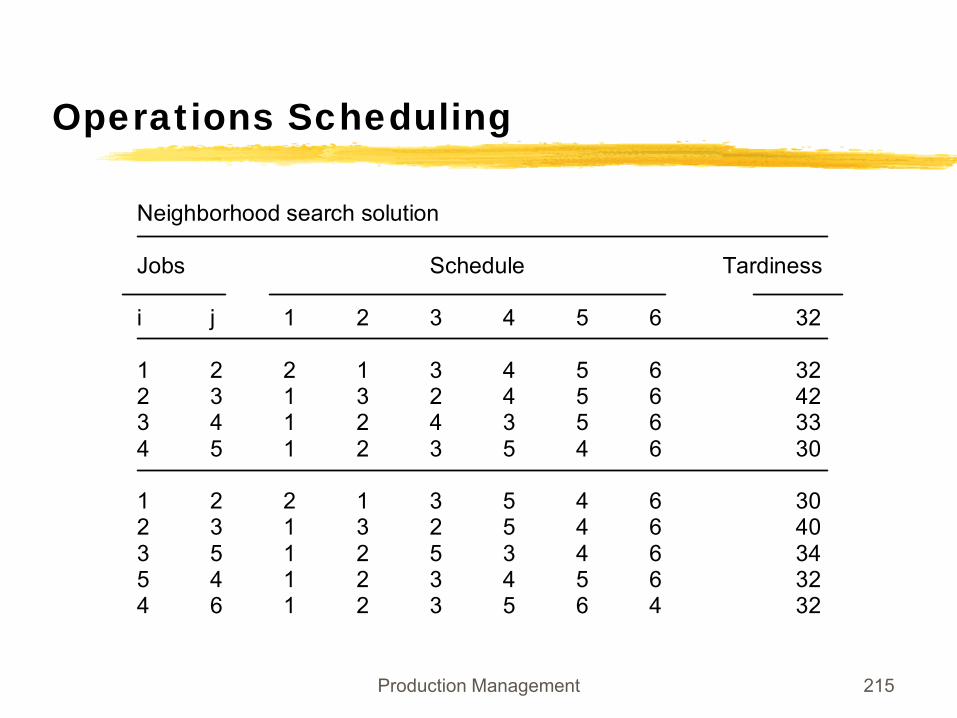
Neighborhood search solution

Jobs Schedule Tardiness

i j 1 2 3 4 5 6 32

1 2 2 1 3 4 5 6 322 3 1 3 2 4 5 6 423 4 1 2 4 3 5 6 334 5 1 2 3 5 4 6 30

1 2 2 1 3 5 4 6 302 3 1 3 2 5 4 6 403 5 1 2 5 3 4 6 345 4 1 2 3 4 5 6 324 6 1 2 3 5 6 4 32



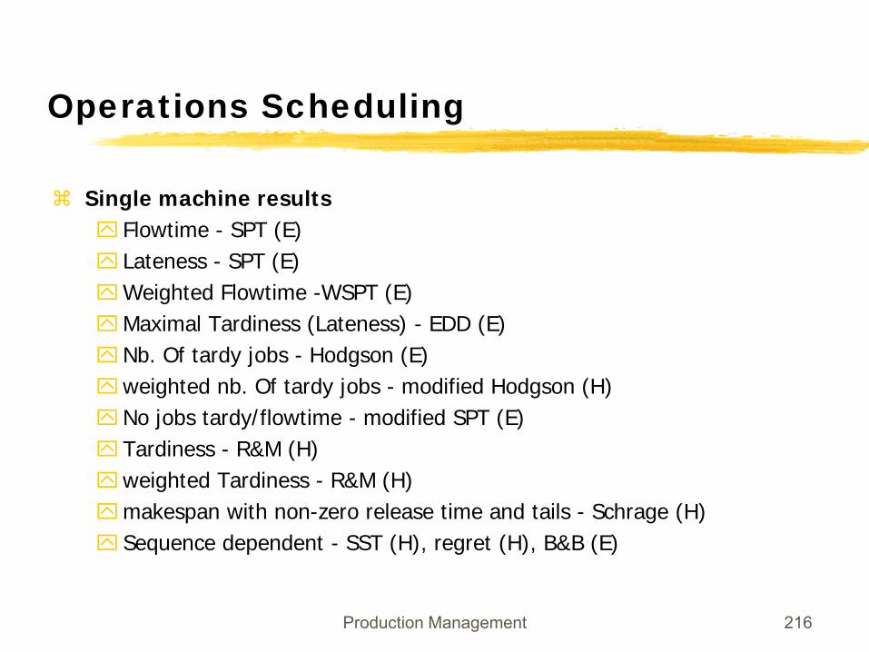
Single machine resultsFlowtime - SPT (E)Lateness - SPT (E)Weighted Flowtime -WSPT (E)Maximal Tardiness (Lateness) - EDD (E)Nb. Of tardy jobs - Hodgson (E)weighted nb. Of tardy jobs - modified Hodgson (H)No jobs tardy/flowtime - modified SPT (E)Tardiness - R&M (H)weighted Tardiness - R&M (H)makespan with non-zero release time and tails - Schrage (H)Sequence dependent - SST (H), regret (H), B&B (E)



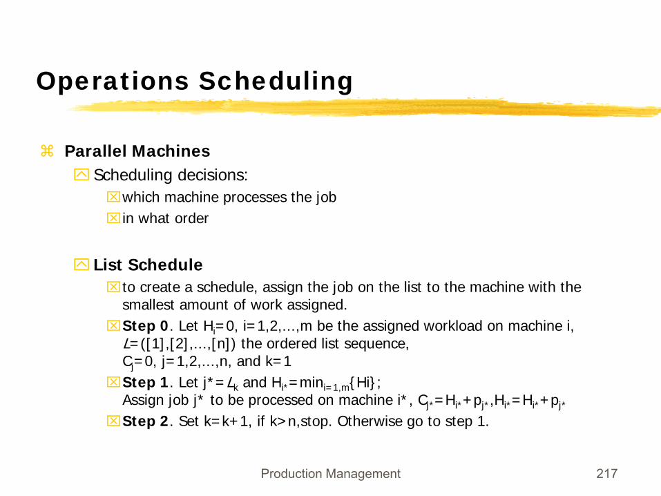
Parallel MachinesScheduling decisions:⌧which machine processes the job⌧in what order

List Schedule⌧to create a schedule, assign the job on the list to the machine with the

smallest amount of work assigned.⌧Step 0. Let Hi=0, i=1,2,...,m be the assigned workload on machine i,

L=([1],[2],...,[n]) the ordered list sequence, Cj=0, j=1,2,...,n, and k=1

⌧Step 1. Let j*=Lk and Hi*=mini=1,m{Hi};Assign job j* to be processed on machine i*, Cj*=Hi*+pj*,Hi*=Hi*+pj*

⌧Step 2. Set k=k+1, if k>n,stop. Otherwise go to step 1.


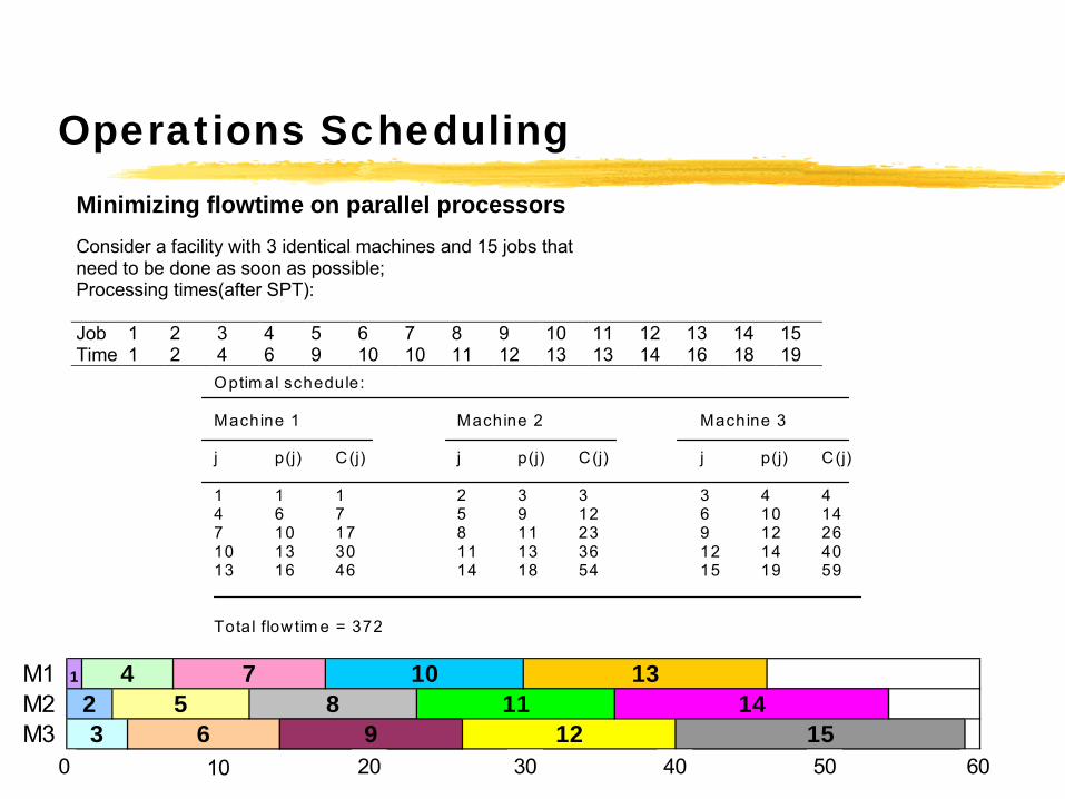
Operations SchedulingMinimizing flowtime on parallel processorsConsider a facility with 3 identical machines and 15 jobs thatneed to be done as soon as possible;Processing times(after SPT):

Job 1 2 3 4 5 6 7 8 9 10 11 12 13 14 15Time 1 2 4 6 9 10 10 11 12 13 13 14 16 18 19

Optim al schedule:

Machine 1 Machine 2 Machine 3

j p(j) C(j) j p(j) C(j) j p(j) C(j)

1 1 1 2 3 3 3 4 44 6 7 5 9 12 6 10 147 10 17 8 11 23 9 12 2610 13 30 11 13 36 12 14 4013 16 46 14 18 54 15 19 59

Total flowtim e = 372

M1 1

M2M3 12

1314

1523

45

6

78

9

1011

0 10 20 30 40 50 60


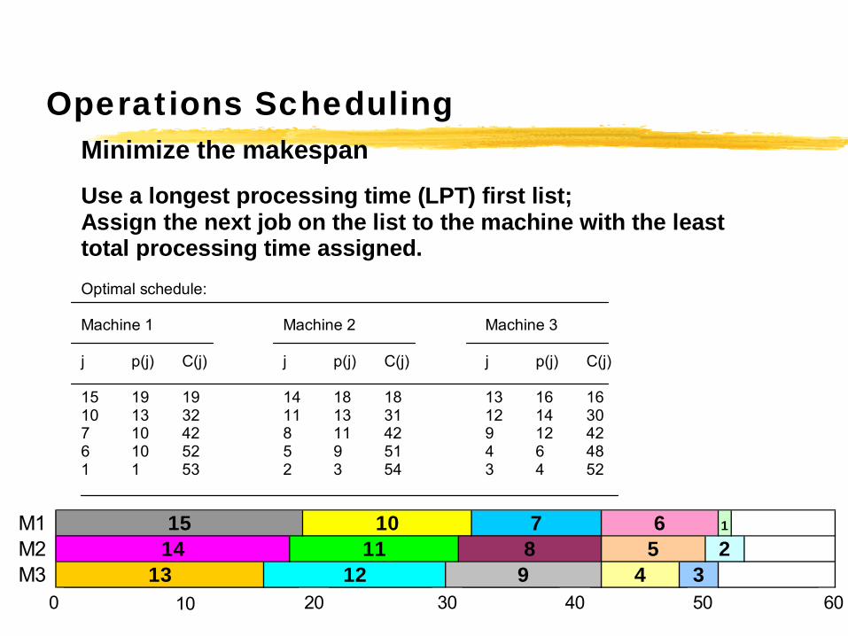
Operations SchedulingMinimize the makespan Use a longest processing time (LPT) first list; Assign the next job on the list to the machine with the least total processing time assigned. Optimal schedule: Machine 1 Machine 2 Machine 3 j p(j) C(j) j p(j) C(j) j p(j) C(j) 15 19 19 14 18 18 13 16 16 10 13 32 11 13 31 12 14 30 7 10 42 8 11 42 9 12 42 6 10 52 5 9 51 4 6 48 1 1 53 2 3 54 3 4 52

M1 1

M2M3

23

1514

13

1011

128

9

7 65

40 10 20 30 40 50 60



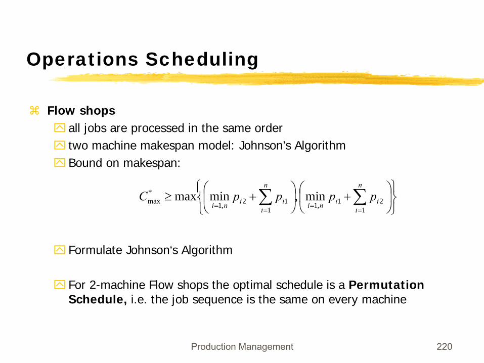
Flow shopsall jobs are processed in the same ordertwo machine makespan model: Johnson’s AlgorithmBound on makespan:

Formulate Johnson‘s Algorithm

For 2-machine Flow shops the optimal schedule is a Permutation Schedule, i.e. the job sequence is the same on every machine

⎭⎬⎫

⎩⎨⎧

⎟⎠

⎞⎜⎝

⎛+⎟

⎠

⎞⎜⎝

⎛+≥ ∑∑

==

==

n

iiini

n

iiini

ppppC1

21,1112,1

*max min,minmax



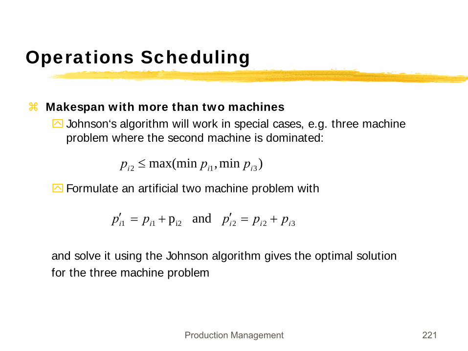
Makespan with more than two machinesJohnson‘s algorithm will work in special cases, e.g. three machine problem where the second machine is dominated:

Formulate an artificial two machine problem with

and solve it using the Johnson algorithm gives the optimal solutionfor the three machine problem

)min,max(min 312 iii ppp ≤

322i211 and p iiiii ppppp +=′+=′



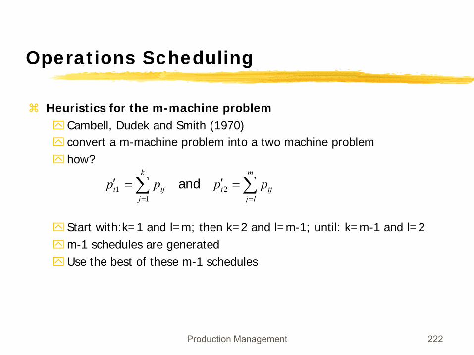
Heuristics for the m-machine problemCambell, Dudek and Smith (1970)convert a m-machine problem into a two machine problemhow?

Start with:k=1 and l=m; then k=2 and l=m-1; until: k=m-1 and l=2m-1 schedules are generatedUse the best of these m-1 schedules

∑∑==

=′=′m

ljiji

k

jiji pppp 2

11 and


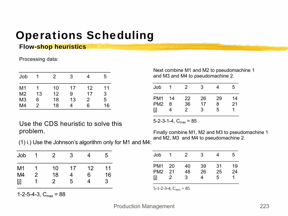
Operations SchedulingFlow-shop heuristics

Processing data:

Job 1 2 3 4 5

M1 1 10 17 12 11M2 13 12 9 17 3M3 6 18 13 2 5M4 2 18 4 6 16

Use the CDS heuristic to solve thisproblem.

(1) i.) Use the Johnson’s algorithm only for M1 and M4:

Job 1 2 3 4 5

M1 1 10 17 12 11M4 2 18 4 6 16[j] 1 2 5 4 3

1-2-5-4-3, Cmax = 88

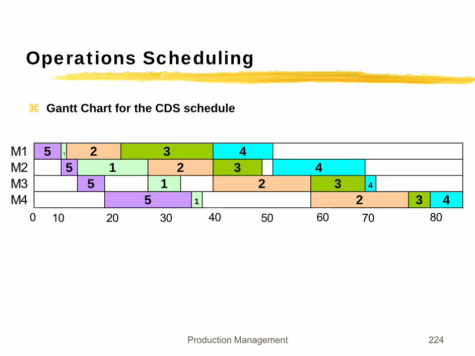
Next combine M1 and M2 to pseudomachine 1 and M3 and M4 to pseudomachine 2. Job 1 2 3 4 5 PM1 14 22 26 29 14 PM2 8 36 17 8 21 [j] 4 2 3 5 1 5-2-3-1-4, Cmax = 85 Finally combine M1, M2 and M3 to pseudomachine 1 and M2, M3 and M4 to pseudomachine 2. Job 1 2 3 4 5 PM1 20 40 39 31 19 PM2 21 48 26 25 24 [j] 2 3 4 5 1 5-1-2-3-4, Cmax = 85



Gantt Chart for the CDS schedule

M1 1

M2M3M4 3 4

4

5 1 25 1 2

2 3 45 1 2 3

54

3

0 10 20 30 40 50 60 70 80



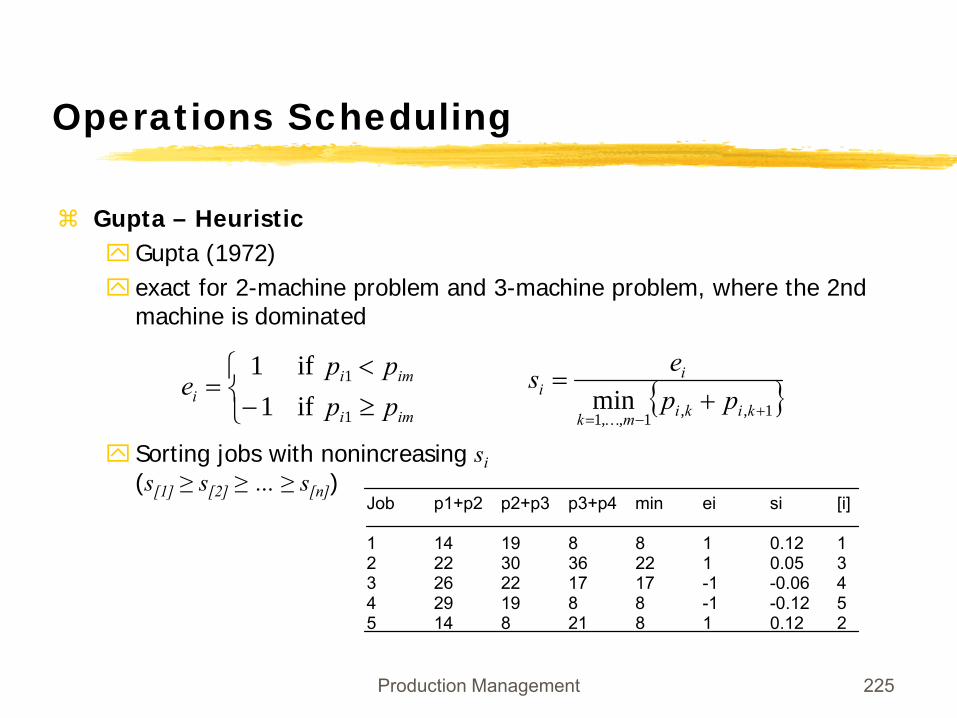
Gupta – HeuristicGupta (1972)exact for 2-machine problem and 3-machine problem, where the 2nd machine is dominated

Sorting jobs with nonincreasing si(s[1] ≥ s[2] ≥ … ≥ s[n])

⎩⎨⎧

≥−<

=imi

imii pp

ppe

1

1

if1 if1

{ }1,,1,,1min +−=

+=

kikimk

ii pp

esK

Job p1+p2 p2+p3 p3+p4 min ei si [i] 1 14 19 8 8 1 0.12 1 2 22 30 36 22 1 0.05 3 3 26 22 17 17 -1 -0.06 4 4 29 19 8 8 -1 -0.12 5 5 14 8 21 8 1 0.12 2



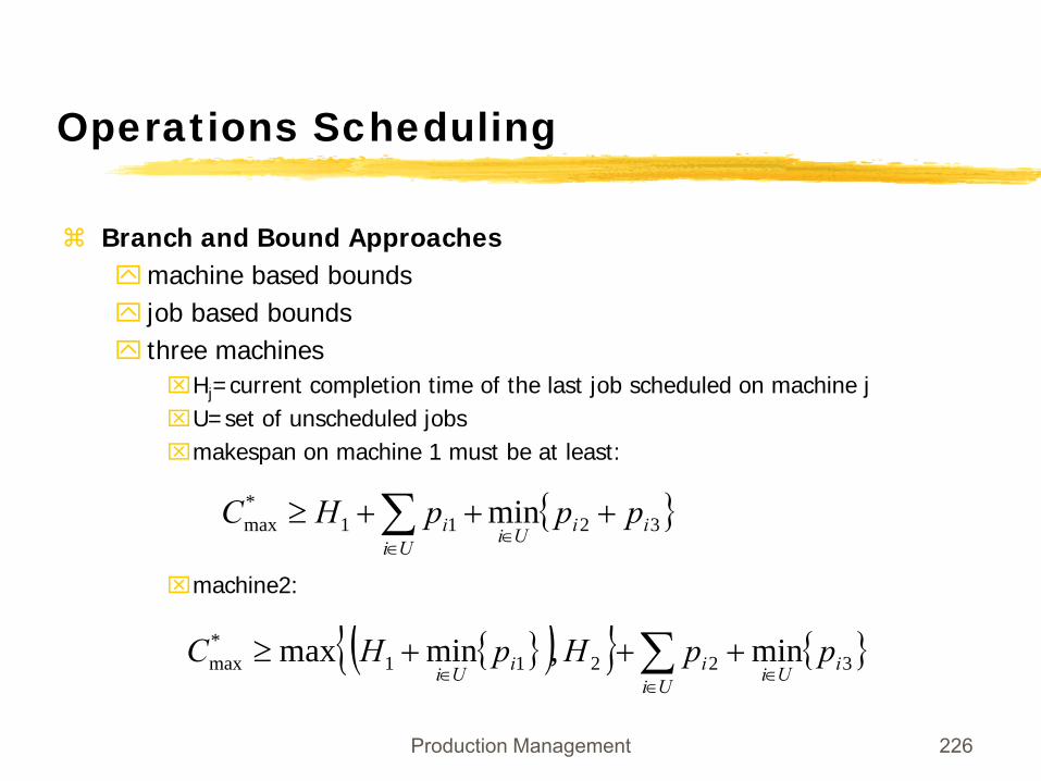
Branch and Bound Approachesmachine based boundsjob based boundsthree machines⌧Hj=current completion time of the last job scheduled on machine j⌧U=set of unscheduled jobs⌧makespan on machine 1 must be at least:

⌧machine2:

{ }3211*max min iiUiUi

i pppHC +++≥∈

∈∑

{ }( ){ } { }∑∈

∈∈+++≥

UiiUiiiUi

ppHpHC 32211*max min,minmax



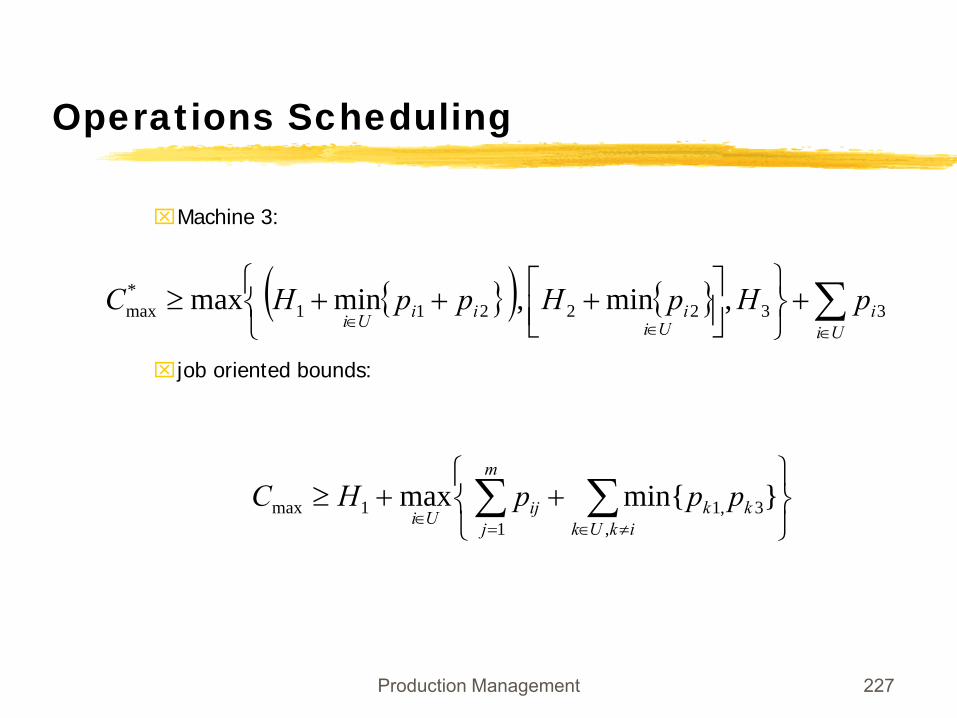
⌧Machine 3:

⌧job oriented bounds:

{ }( ) { } ∑∈∈∈

+⎭⎬⎫

⎩⎨⎧

⎥⎦⎤

⎢⎣⎡ +++≥

Uii

UiiiiUi

pHpHppHC 3322211*max ,min,minmax

⎭⎬⎫

⎩⎨⎧

++≥ ∑∑≠∈=

∈ ikUkkk

m

jijUi

pppHC,

3,11

1max }min{max



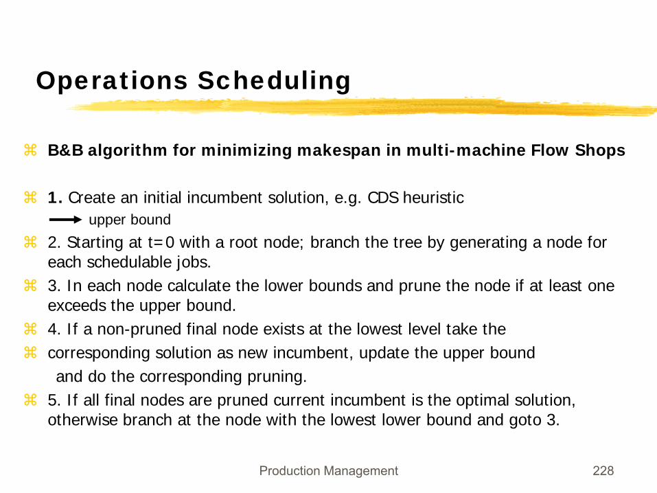
B&B algorithm for minimizing makespan in multi-machine Flow Shops

1. Create an initial incumbent solution, e.g. CDS heuristicupper bound

2. Starting at t=0 with a root node; branch the tree by generating a node foreach schedulable jobs.3. In each node calculate the lower bounds and prune the node if at least oneexceeds the upper bound.4. If a non-pruned final node exists at the lowest level take thecorresponding solution as new incumbent, update the upper boundand do the corresponding pruning.

5. If all final nodes are pruned current incumbent is the optimal solution, otherwise branch at the node with the lowest lower bound and goto 3.


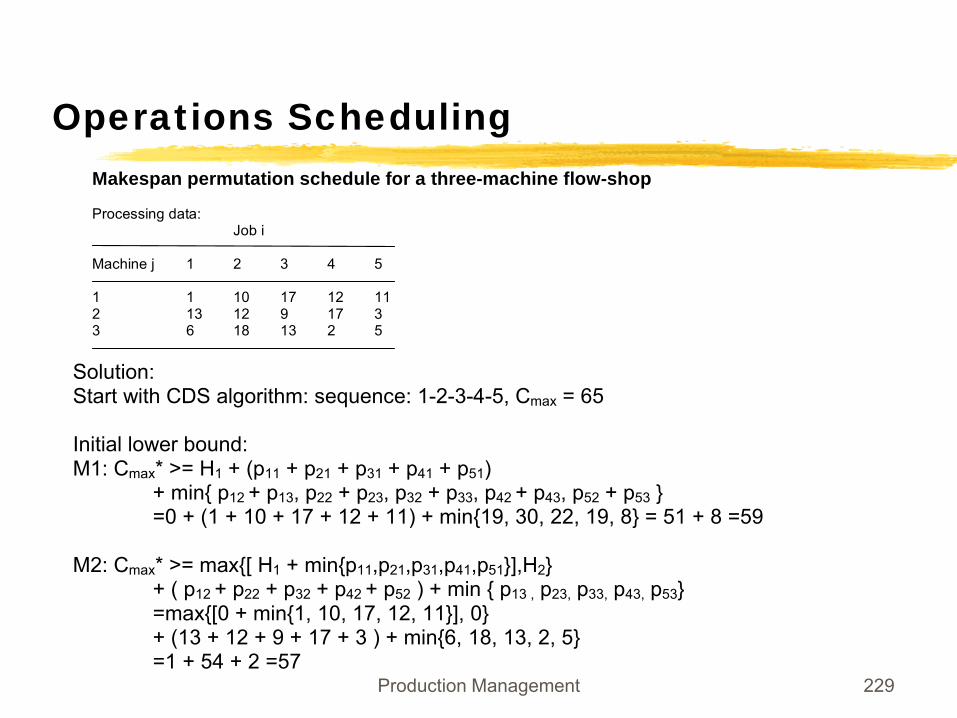
Operations SchedulingMakespan permutation schedule for a three-machine flow-shop

Processing data:Job i

Machine j 1 2 3 4 5

1 1 10 17 12 112 13 12 9 17 33 6 18 13 2 5

Solution: Start with CDS algorithm: sequence: 1-2-3-4-5, Cmax = 65 Initial lower bound: M1: Cmax* >= H1 + (p11 + p21 + p31 + p41 + p51) + min{ p12 + p13, p22 + p23, p32 + p33, p42 + p43, p52 + p53 } =0 + (1 + 10 + 17 + 12 + 11) + min{19, 30, 22, 19, 8} = 51 + 8 =59 M2: Cmax* >= max{[ H1 + min{p11,p21,p31,p41,p51}],H2} + ( p12 + p22 + p32 + p42 + p52 ) + min { p13 , p23, p33, p43, p53} =max{[0 + min{1, 10, 17, 12, 11}], 0} + (13 + 12 + 9 + 17 + 3 ) + min{6, 18, 13, 2, 5} =1 + 54 + 2 =57


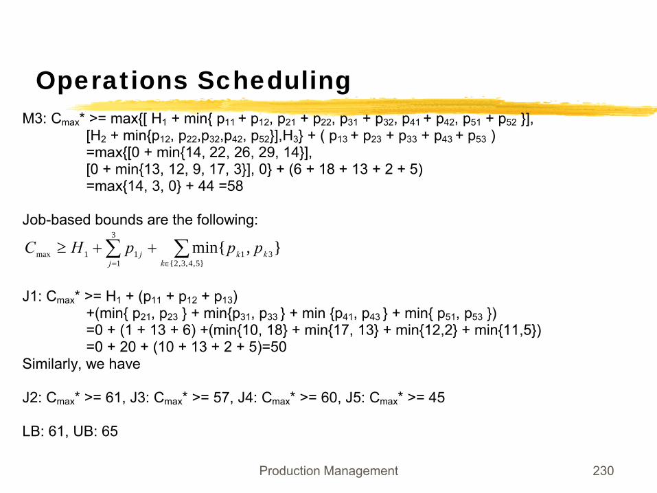
Operations SchedulingM3: Cmax* >= max{[ H1 + min{ p11 + p12, p21 + p22, p31 + p32, p41 + p42, p51 + p52 }], [H2 + min{p12, p22,p32,p42, p52}],H3} + ( p13 + p23 + p33 + p43 + p53 ) =max{[0 + min{14, 22, 26, 29, 14}], [0 + min{13, 12, 9, 17, 3}], 0} + (6 + 18 + 13 + 2 + 5) =max{14, 3, 0} + 44 =58 Job-based bounds are the following:

J1: Cmax* >= H1 + (p11 + p12 + p13) +(min{ p21, p23 } + min{p31, p33 } + min {p41, p43 } + min{ p51, p53 }) =0 + (1 + 13 + 6) +(min{10, 18} + min{17, 13} + min{12,2} + min{11,5}) =0 + 20 + (10 + 13 + 2 + 5)=50 Similarly, we have J2: Cmax* >= 61, J3: Cmax* >= 57, J4: Cmax* >= 60, J5: Cmax* >= 45 LB: 61, UB: 65

∑∑∈=

++≥}5,4,3,2{

31

3

111max },min{

kkk

jj pppHC


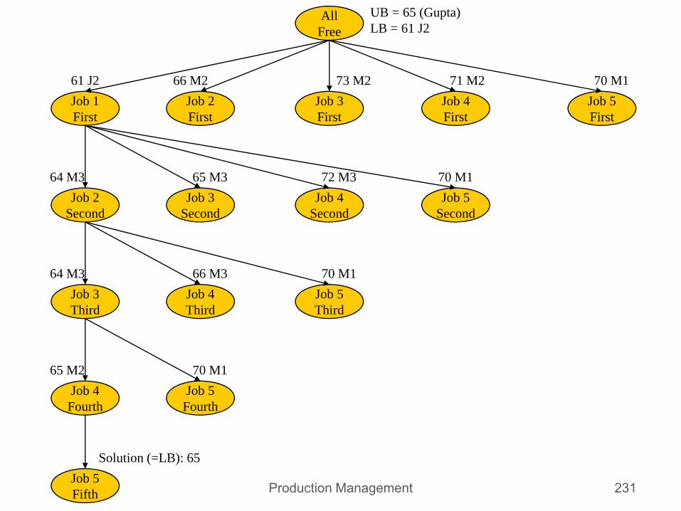
AllFree

UB = 65 (Gupta)LB = 61 J2

Job 1First

Job 2First

Job 3First

Job 4First

Job 5First

61 J2 66 M2 73 M2 71 M2 70 M1

Job 2Second

Job 3Second

Job 4Second

Job 5Second

64 M3 65 M3 72 M3 70 M1

Job 3Third

Job 4Third

Job 5Third

64 M3 66 M3 70 M1

Job 4Fourth

Job 5Fourth

65 M2 70 M1

Job 5Fifth

Solution (=LB): 65


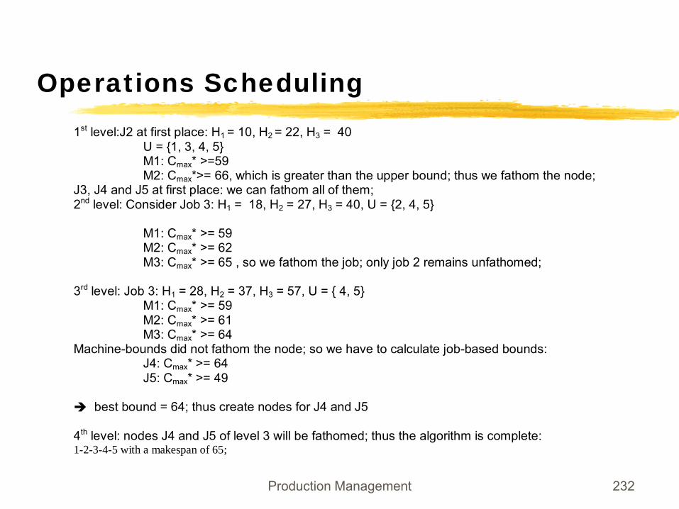
Operations Scheduling1st level:J2 at first place: H1 = 10, H2 = 22, H3 = 40

U = {1, 3, 4, 5}M1: Cmax* >=59M2: Cmax*>= 66, which is greater than the upper bound; thus we fathom the node;

J3, J4 and J5 at first place: we can fathom all of them;2nd level: Consider Job 3: H1 = 18, H2 = 27, H3 = 40, U = {2, 4, 5}

M1: Cmax* >= 59M2: Cmax* >= 62M3: Cmax* >= 65 , so we fathom the job; only job 2 remains unfathomed;

3rd level: Job 3: H1 = 28, H2 = 37, H3 = 57, U = { 4, 5}M1: Cmax* >= 59M2: Cmax* >= 61M3: Cmax* >= 64

Machine-bounds did not fathom the node; so we have to calculate job-based bounds:J4: Cmax* >= 64J5: Cmax* >= 49

best bound = 64; thus create nodes for J4 and J5

4th level: nodes J4 and J5 of level 3 will be fathomed; thus the algorithm is complete:1-2-3-4-5 with a makespan of 65;



Job Shopsdifferent routings for different jobsprecedence constraints(n!)m possible schedules



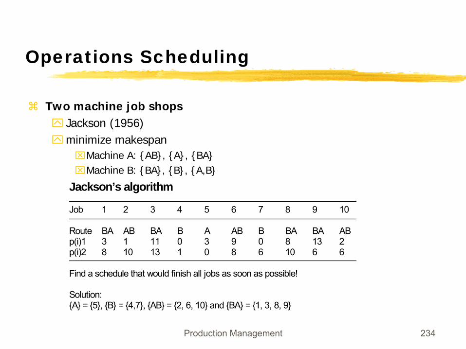
Two machine job shopsJackson (1956)minimize makespan⌧Machine A: {AB}, {A}, {BA}⌧Machine B: {BA}, {B}, {A,B}

Jackson’s algorithm

Job 1 2 3 4 5 6 7 8 9 10

Route BA AB BA B A AB B BA BA ABp(i)1 3 1 11 0 3 9 0 8 13 2p(i)2 8 10 13 1 0 8 6 10 6 6

Find a schedule that would finish all jobs as soon as possible!

Solution:{A} = {5}, {B} = {4,7}, {AB} = {2, 6, 10} and {BA} = {1, 3, 8, 9}


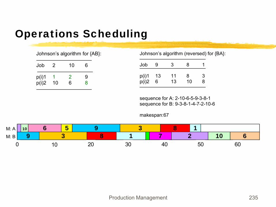
Operations SchedulingJohnson’s algorithm for {AB}:

Job 2 10 6

p(i)1 1 2 9p(i)2 10 6 8

Johnson’s algorithm (reversed) for {BA}:

Job 9 3 8 1

p(i)1 13 11 8 3p(i)2 6 13 10 8

sequence for A: 2-10-6-5-9-3-8-1sequence for B: 9-3-8-1-4-7-2-10-6

makespan:67

M: A

M: B 2 10 69 3 8 110 6 5 9 3 8 1

70 10 20 30 40 50 60



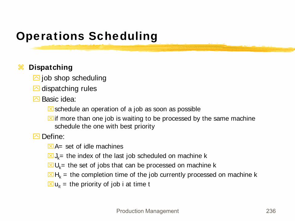
Dispatchingjob shop schedulingdispatching rulesBasic idea:⌧schedule an operation of a job as soon as possible⌧if more than one job is waiting to be processed by the same machine

schedule the one with best priority

Define:⌧A= set of idle machines⌧Jk= the index of the last job scheduled on machine k⌧Uk= the set of jobs that can be processed on machine k⌧Hk = the completion time of the job currently processed on machine k⌧uit = the priority of job i at time t



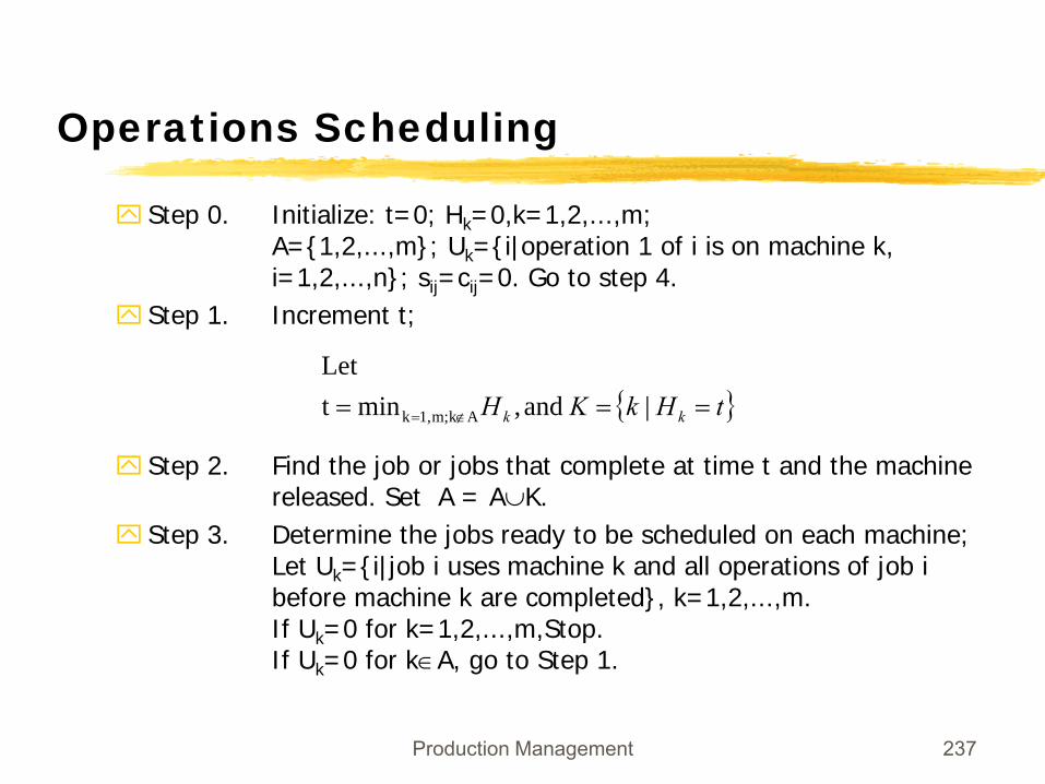
Step 0. Initialize: t=0; Hk=0,k=1,2,...,m;A={1,2,...,m}; Uk={i|operation 1 of i is on machine k, i=1,2,...,n}; sij=cij=0. Go to step 4.

Step 1. Increment t;

Step 2. Find the job or jobs that complete at time t and the machine released. Set A = A∪K.

Step 3. Determine the jobs ready to be scheduled on each machine;Let Uk={i|job i uses machine k and all operations of job i before machine k are completed}, k=1,2,...,m.If Uk=0 for k=1,2,...,m,Stop.If Uk=0 for k∈A, go to Step 1.

{ }tHkKH kk === ∉= | and,mintLet

Akm;1,k



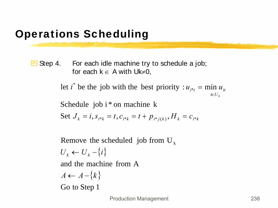
Step 4. For each idle machine try to schedule a job;for each k ∈ A with Uk≠0,

{}

{ }1 Step toGo

A from machine theand

Ufrom job scheduled theRemove

,,,Set k machineon *i job Schedule

min:prioritybest with thejob thebe let

k

*)(***

*

kAA

iUU

cHptctsiJ

uui

kk

kikkjikikik

Uiiti*t

k

−←

−←

=+===

=∈



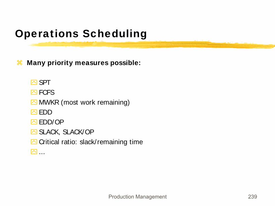
Many priority measures possible:

SPTFCFSMWKR (most work remaining)EDDEDD/OPSLACK, SLACK/OPCritical ratio: slack/remaining time...



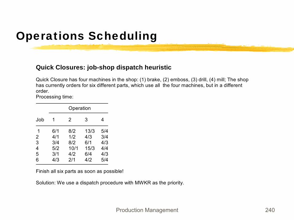
Quick Closures: job-shop dispatch heuristic

Quick Closure has four machines in the shop: (1) brake, (2) emboss, (3) drill, (4) mill; The shophas currently orders for six different parts, which use all the four machines, but in a differentorder.Processing time:

Operation

Job 1 2 3 4

1 6/1 8/2 13/3 5/42 4/1 1/2 4/3 3/43 3/4 8/2 6/1 4/34 5/2 10/1 15/3 4/45 3/1 4/2 6/4 4/36 4/3 2/1 4/2 5/4

Finish all six parts as soon as possible!

Solution: We use a dispatch procedure with MWKR as the priority.



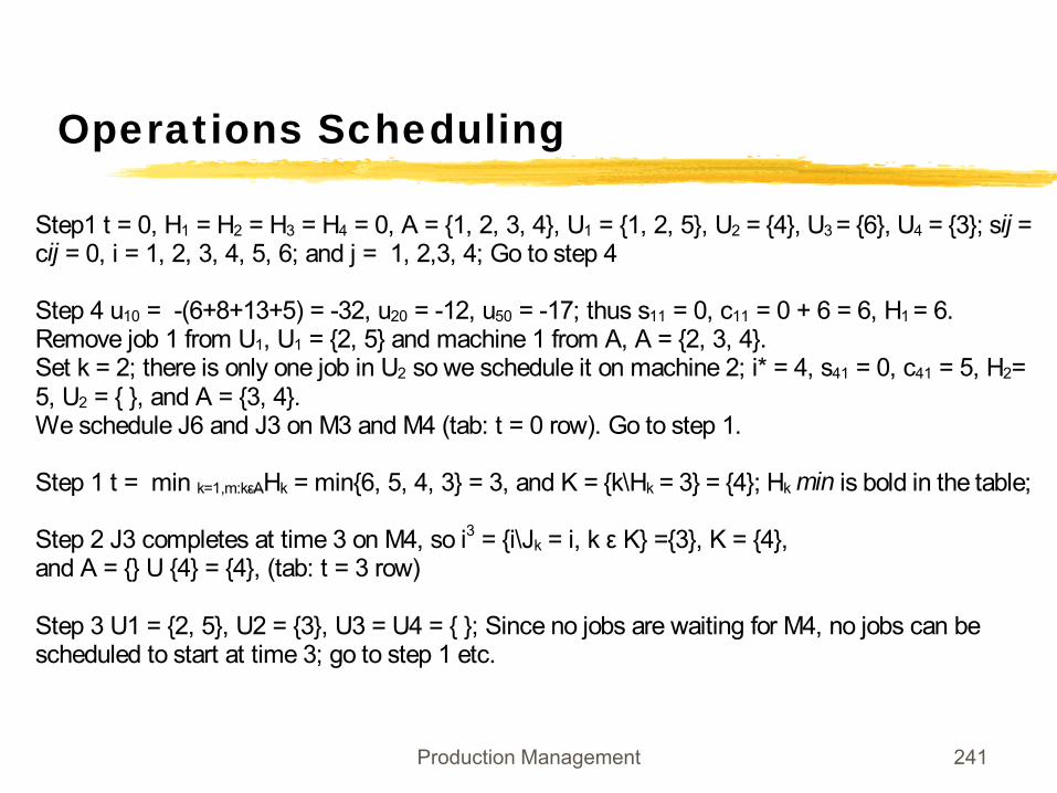
Step1 t = 0, H1 = H2 = H3 = H4 = 0, A = {1, 2, 3, 4}, U1 = {1, 2, 5}, U2 = {4}, U3 = {6}, U4 = {3}; sij = cij = 0, i = 1, 2, 3, 4, 5, 6; and j = 1, 2,3, 4; Go to step 4 Step 4 u10 = -(6+8+13+5) = -32, u20 = -12, u50 = -17; thus s11 = 0, c11 = 0 + 6 = 6, H1 = 6. Remove job 1 from U1, U1 = {2, 5} and machine 1 from A, A = {2, 3, 4}. Set k = 2; there is only one job in U2 so we schedule it on machine 2; i* = 4, s41 = 0, c41 = 5, H2= 5, U2 = { }, and A = {3, 4}. We schedule J6 and J3 on M3 and M4 (tab: t = 0 row). Go to step 1. Step 1 t = min k=1,m:kεAHk = min{6, 5, 4, 3} = 3, and K = {k\Hk = 3} = {4}; Hk min is bold in the table; Step 2 J3 completes at time 3 on M4, so i3 = {i\Jk = i, k ε K} ={3}, K = {4}, and A = {} U {4} = {4}, (tab: t = 3 row) Step 3 U1 = {2, 5}, U2 = {3}, U3 = U4 = { }; Since no jobs are waiting for M4, no jobs can be scheduled to start at time 3; go to step 1 etc.



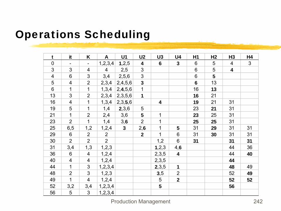
t it K A U1 U2 U3 U4 H1 H2 H3 H40 - - 1,2,3,4 1,2,5 4 6 3 6 5 4 33 3 4 4 2,5 3 6 5 44 6 3 3,4 2,5,6 3 6 55 4 2 2,3,4 2,4,5,6 3 6 136 1 1 1,3,4 2,4,5,6 1 16 13

13 3 2 2,3,4 2,3,5,6 1 16 2116 4 1 1,3,4 2,3,5,6 4 19 21 3119 5 1 1,4 2,3,6 5 23 21 3121 1 2 2,4 3,6 5 1 23 25 3123 2 1 1,4 3,6 2 1 25 25 3125 6,5 1,2 1,2,4 3 2,6 1 5 31 29 31 3129 6 2 2 2 1 6 31 30 31 3130 2 2 2 1,2 6 31 31 3131 3,4 1,3 1,2,3 1,2,3 4,6 44 3636 6 4 1,2,4 2,3,5 4 44 4040 4 4 1,2,4 2,3,5 4444 1 3 1,2,3,4 2,3,5 1 48 4948 2 3 1,2,3 3,5 2 52 4949 1 4 1,2,4 5 2 52 5252 3,2 3,4 1,2,3,4 5 5656 5 3 1,2,3,4



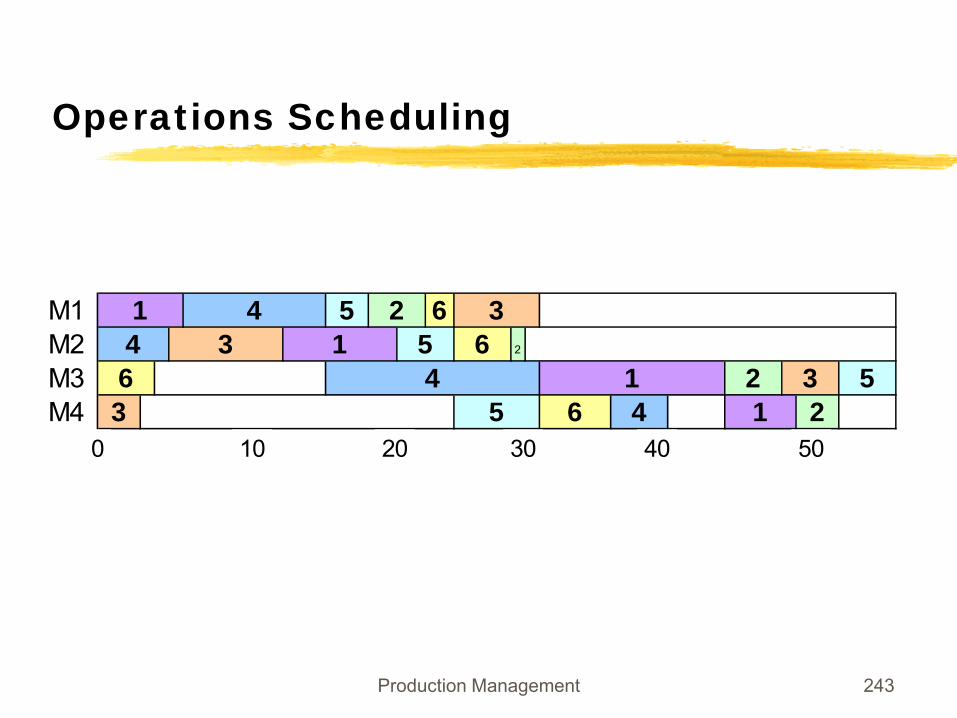
M1M2 2

M3M4 6 4 1 2

33 1 5 6

1 5 2 64463

45

1 2 3 5

0 10 20 30 40 50

Chapter 10

Section 5.5: Bottleneck Scheduling



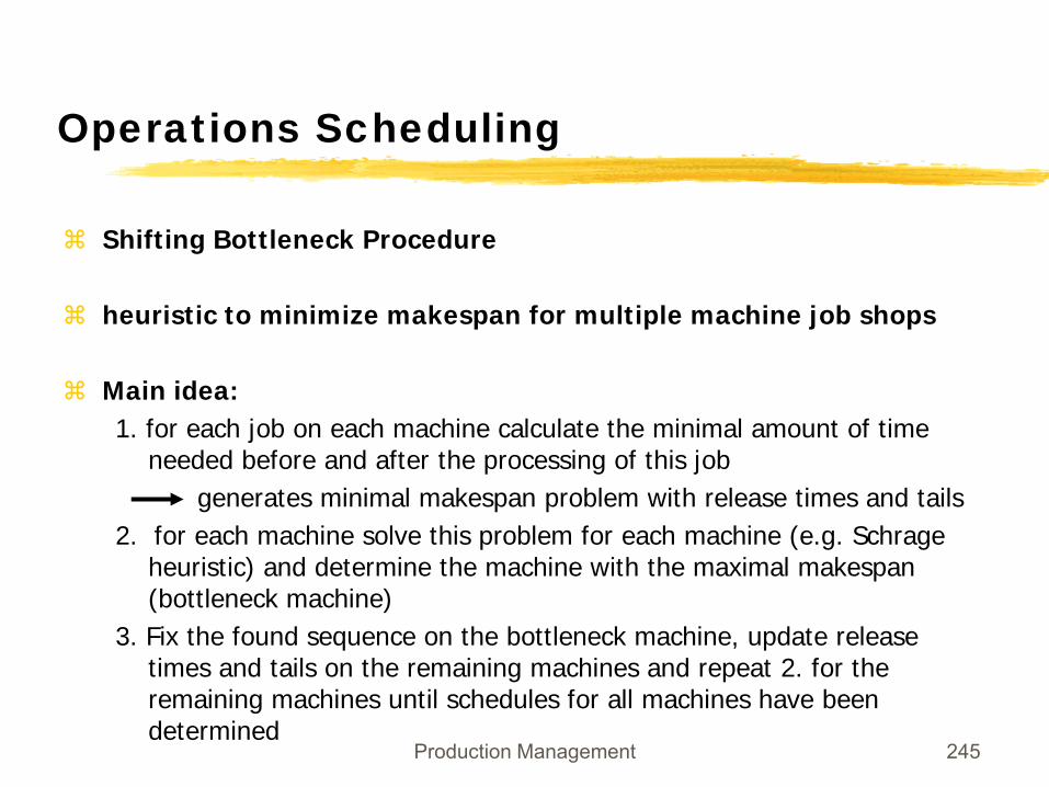
Shifting Bottleneck Procedure

heuristic to minimize makespan for multiple machine job shops

Main idea:1. for each job on each machine calculate the minimal amount of time

needed before and after the processing of this job generates minimal makespan problem with release times and tails

2. for each machine solve this problem for each machine (e.g. Schrage heuristic) and determine the machine with the maximal makespan (bottleneck machine)

3. Fix the found sequence on the bottleneck machine, update release times and tails on the remaining machines and repeat 2. for the remaining machines until schedules for all machines have been determined



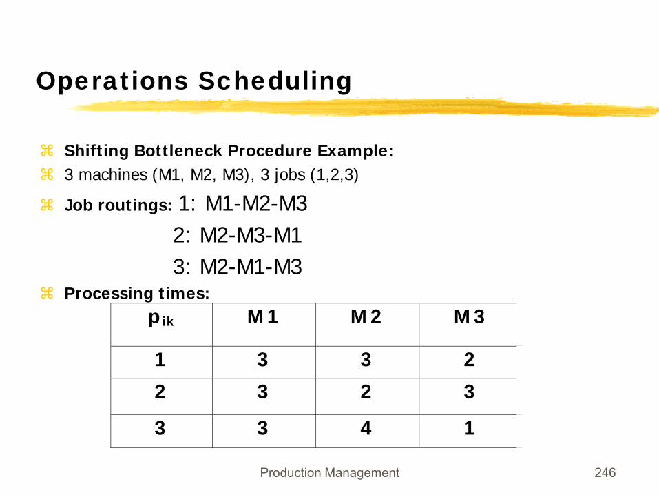
Shifting Bottleneck Procedure Example:3 machines (M1, M2, M3), 3 jobs (1,2,3)

Job routings: 1: M1-M2-M32: M2-M3-M13: M2-M1-M3

Processing times:pik M1 M2 M3

1 3 3 2

2 3 2 3

3 3 4 1



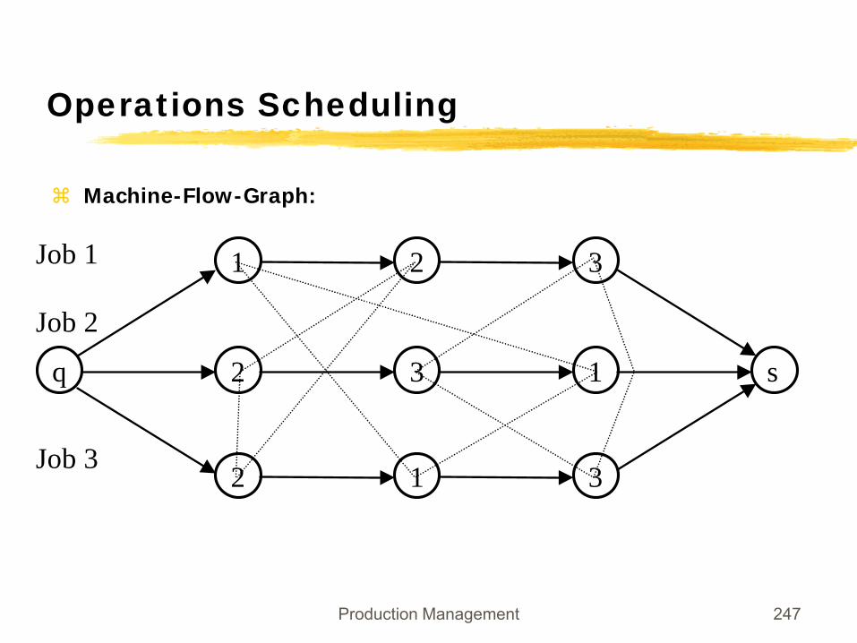
Machine-Flow-Graph:

2

2

1

3

1

2

3

3

sq 1

Job 1

Job 2

Job 3



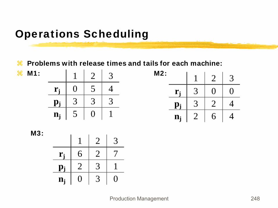
Problems with release times and tails for each machine:M1: M2:

M3:

1 2 3rj 0 5 4pj 3 3 3nj 5 0 1

1 2 3rj 3 0 0pj 3 2 4nj 2 6 4

1 2 3rj 6 2 7pj 2 3 1nj 0 3 0



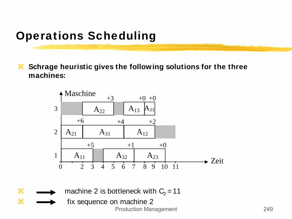
Schrage heuristic gives the following solutions for the three machines:

machine 2 is bottleneck with C2 =11fix sequence on machine 2

A31 A12

Maschine

11109654

+2+4+6

2

320Zeit

A21

87

A32 A23

+0+1+51 A11

A33A13

+0+0+33 A22



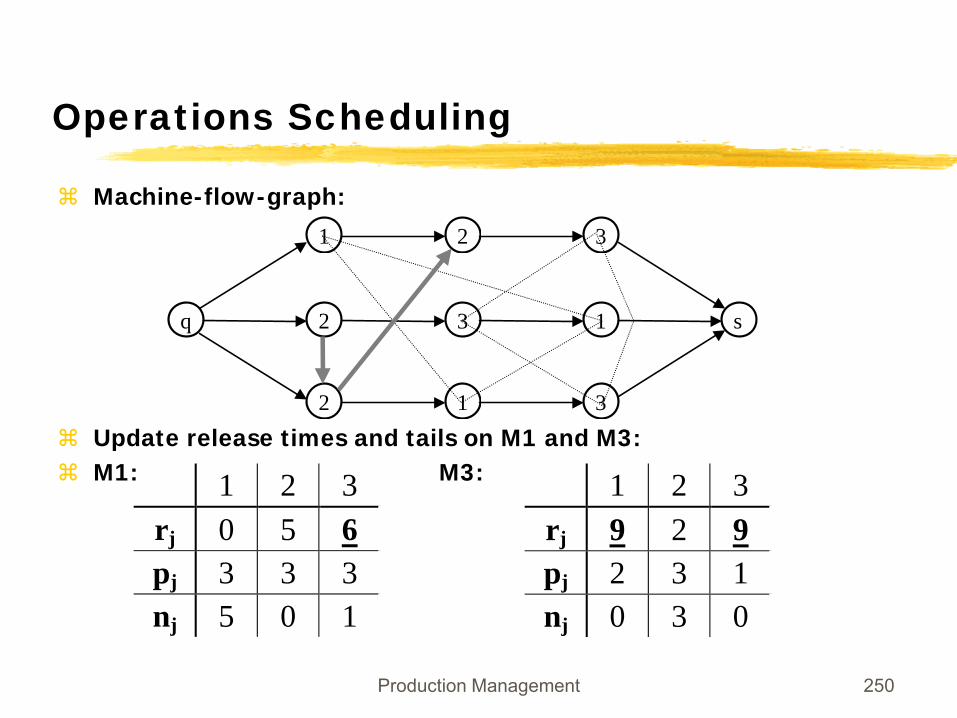
Machine-flow-graph:

Update release times and tails on M1 and M3:M1: M3:

2

2

1

3

1

2

3

3

sq 1

1 2 3rj 0 5 6pj 3 3 3nj 5 0 1

1 2 3rj 9 2 9pj 2 3 1nj 0 3 0



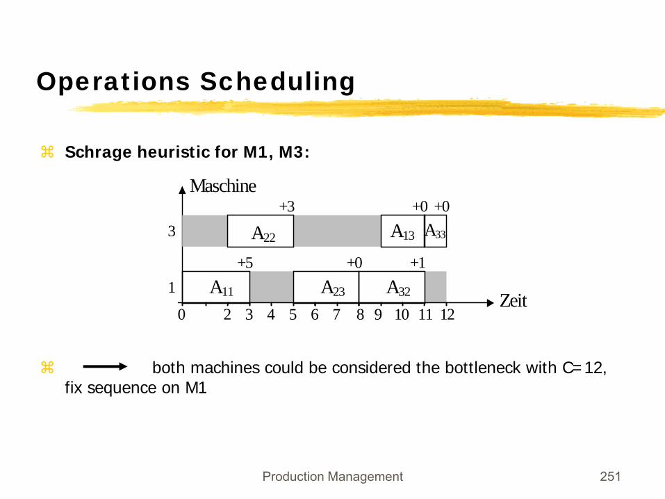
Schrage heuristic for M1, M3:

both machines could be considered the bottleneck with C=12, fix sequence on M1

3

Maschine

11109654320Zeit

87

A32A23

+0 +1+51 A11

A33A13

+0+0+3

A22

12


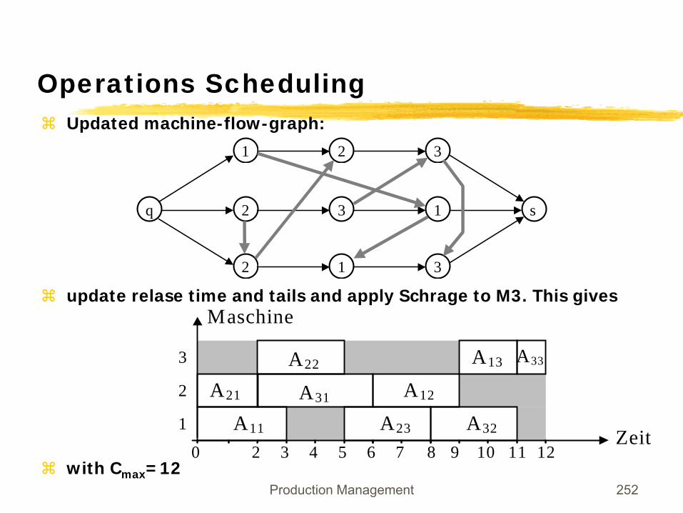
Operations SchedulingUpdated machine-flow-graph:

update relase time and tails and apply Schrage to M3. This gives

with Cmax=12

2

2

1

3

1

2

3

3

sq 1

3

Maschine

11109654320Zeit

87

A32A231 A11

A33A13A22

12

2 A12A21 A31



Finite Capacity Scheduling

⌧MRP systems generally assume constant lead times, ignore setups

⌧MRP plans might be unrealistic

⌧Traditionally problem hiden by inventory and excess capacity

⌧Reducing Inventory and capacity makes finite capacity scheduling crucial

⌧Computer-assisted finitie capacity scheduling systems rather than manual scheduling by foreman



Work to do: 8.3abcde, 8.4, 8.5, 8.6, 8.10, 8.14, 8.16, 8.18 (with the following due dates: 42, 50, 12, 63, 23, 34, 36, 42, 54, 32) 8.30ab, 8.32abc, 8.36ab, 8.43, 8.44, 8.49ab, 8.51ab, 8.56, 8.57 (apply shifting bottleneck procedure)

Minicase: Ilana Designs

operations scheduling - · pdf filechapter 8 operations scheduling. production management....

Documents