1

OPERATIONS HANDBOOK - OZONE OBSERVATIONS WITH A DOBSON SPECTROPHOTOMETER

by

W. D. Komhyr Prepared for the World Meteorological Organization Global Ozone Research and Monitoring

Project

June, 1980

Revised September, 2006

Robert D. Evans

NOAA/ESRL Global Monitoring Division

Table of Contents Page Foreword 1. Introduction 4 2. Ozone Measurement Principle and Theory 6 2.1 Total Ozone Observations 6 2.2 Ozone Vertical Distribution (Umkehr) Observations 8 2.3 Principle of Operation of the Spectrophotometer 8 3. Calibration of a Dobson Spectrophotometer 11 3.1 Relative Calibration 11 3.1.1 Adjustment of the Optics 11 3.1.2 Q Calibration 11 3.1.3 Optical Wedge Calibration 11 3.2 Absolute Calibration 12 3.3 Maintaining a Spectrophotometer in Calibration 12 4. Routine Spectrophotometer Tests and Maintenance 13 4.1 Purpose of Spectrophotometer Tests 13 4.2 Frequency of Tests 13 4.3 Recording of Test Data 13 4.4 Test Procedures 14 4.4.1 Mercury Lamp Tests 15 4.4.2 Standard Lamp Tests 16 5. Instrument Maintenance and Repair 19 5.1 Adjustment of Instrument Electronics 19 5.2 Decrease in Shutter-Motor Speed 19 5.3 Radio-Frequency Pickup 20

2

5.4 Ground loops and other problems 20 5.5 Mechanical Shock Avoidance 20 5.6 Instrument Temperature Control 21 5.7 Renewing the Desiccant 21 5.8 Cleaning Optical Components 21 5.9 Exposure of Photomultiplier to Intense Light 22 5.10 Replacing Standard Lamps 22 5.11 Replacing a Photomultiplier Tube 23 6. Observations 24 6.1 Observation Shelters 24 6.2 Observations of Total Ozone Amount 24 6.2.1 Observation Types 24 6.2.2 Times of Routine Ozone Measurements 26 6.2.3 Recording Observational Data 27 6.2.4 Observing Methods 28 6.2.4.1 AD-DSGQP Observations 29 6.2.4.2 AD-DSGQP* Observations 31 6.2.4.3 CD-DSGQP Observations 31 6.2.4.4 AD-ZB Observations 31 6.2.4.5 AD-ZC Observations 31 6.2.4.6 CD-ZB and CD-ZC Observations 32 6.2.4.7 CC'-ZB and CC'-ZC Observations 32 6.2.4.8 AD-DSFI and CD-DSFI Observations 32 6.2.4.9 AD-RMFI and CD-RMFI Observations 33 6.3 Umkehr Observations 33 6.3.1 Observing Times 34 6.3.2 Recording Observational Data 34 6.3.3 Observing Procedures 34 6.4 Special Observations 35 6.4.1 Observations Made to Check the Spectrophotometer

Calibration at A, C, and D Wavelengths 35 6.4.2 Observations Made to Correct Empirical Charts

or Zenith Polynomials 35 6.4.3 Determination of Focused Image Corrections 36 6.4.4 Multiplying Factors Used in Reducing CDDSGQP

Values to the ADDSGQP Level 36 7. Reduction of Ozone Data 38 7.1 Calculations of Total Ozone from Measurements on Direct Sun or Moon 39 7.1.1 Ozone Absorption Coefficients 40 7.1.2 Rayleigh Scattering Coefficients 40 7.1.3 Particle Scattering Coefficients 41 7.1.4 Computation of mu 41 7.1.5 Values of m and p/po 42 7.1.6 Computation of Cosine (Zenith Angle) for Sun and Moon 42 7.2 Calculation of Ozone Amounts from Measurements on

the Clear Zenith Sky 42 7.2.1 AD-ZB Observation 43 7.2.2 CD-ZB Observations 43 7.2.3 CC'-ZB Observations 43

3

7.3 Calculation of Ozone Amounts from Measurements on the Cloudy Zenith Sky 44

7.3.1 AD-ZC Observations 44 7.3.2 CD-ZC Observations 44 7.3.3 CC'-ZC Observations 44 7.4 Reduction of Umkehr Data 45 8. Coding and Archiving Ozone Data 47 References 48 Acknowledgements 50 List of contacts for assistance 51 Appendix A. Determination of Q Setting Tables for Standard Wavelengths 53 Appendix B. Correcting the Table of Settings of Q 59 Appendix C. Calibration of the Dobson Spectrophotometer Optical Wedge 61 Appendix D. Calibrating a Spectrophotometer on an Absolute Scale 69 Appendix E. Determination of Corrections to N Tables from

Standard Lamp Test Data 74 Appendix F. Computation of Cosine Z and mu for Sun and Moon 76 Appendix G. Introduction to Principles of Astronomy 82 Appendix H. Concept of Time 88

4

OZONE OBSERVATIONS WITH A DOBSON SPECTROPHOTOMETER

What follows is the original introduction to the Report No.6: It is impossible to write a manual such as this one without attesting to the impressive contribution made by G.M.B. Dobson in the field of ozone spectrophotometry. Much of the information con-tained in this manual has been obtained, with the kind permission of Pergamon Press, Inc. (Lon-don, New York, Paris), from a pair of handbooks prepared by Dobson (1957a, 1957b). These handbooks have served as primary sources of information for operators of Dobson spectropho-tometers since the International Geophysical Year (1957-1959). In recent years, a considerable amount of on-the-job experience has been acquired by a number of research workers operating the Dobson instruments throughout the world. Improved instrument calibration and data reduction methods have evolved; observational procedures have become standardized; original electro-mechanical components in many of the instruments have been re-placed with modern electronics; and much has been learned about the care of the instruments. In outlining methods for the operation, calibration, and care of Dobson spectrophotometers, and for reduction of total ozone and ozone vertical distribution (Umkehr) data, this manual contains up-dated as well as new information. Its purpose is to continue the tradition set by the Dobson hand-books in providing guidance for standardizing Dobson spectrophotometer operating procedures within the global total ozone station network. Although this manual constitutes a self-contained set of instructions for operators of Dobson in-struments, reference is made in it to the two 1957 Dobson handbooks, with which ozone observ-ers should become familiar. Additional valuable information concerning the accuracy of Dobson spectrophotometer observations is contained in a publication by Dobson and Normand (1962). Observers will find useful, also, a series of working papers by Dobson that have been edited by Walshaw for the Institute of Geophysics, Polish Academy of Sciences (Walshaw, 1975). These words are as true 25 years later as when they were written. Ozone depletion and the world’s response in form of the Montreal Protocols (http://www.undp.org/seed/eap/montreal/montreal.htm) have made the future measurements from these instruments just as important as in the past. The instruments remain the same optically, but advances in electronics, and especially computer power have lead to automated and semi-automated instruments. The 1980 manual will continue to be the basis for operations of the in-strument, but with additions and comments based on experiences of the last 25 years, and changes in the world – as shown by the link to a web page above. The new report “No.6” will have a dy-namic, web-based component (http://www.chmi.cz/meteo/ozon/dobsonweb/welcome.htm).

5

This manual serves a number of functions, describing:

• How to operate the instrument and verify it is operating correctly. “Operate” means what does it do, how turn it on, how to verify that it is working correctly, etc, and is what an operator does.

• How to make the measurements to produce total ozone values. This is the function of an observer.

• How to process and report the observations using unified and validated algorithms and PC software tools. This is the function of both an observer and of the program manager.

• How to combine the operation of the instrument, analysis of the measurements, and then to connect these measurements with the other instruments and measurements in the global network. This is the function of the program manager.

6

OZONE MEASUREMENT PRINCIPLE AND THEORY 2.1 Total Ozone Observations Total ozone observations are made with the Dobson spectrophotometer by measuring the relative intensities of selected pairs of ultraviolet wavelengths, called the A, B*, C, C', and D wavelength pairs, emanating from the sun, moon or zenith sky. The A wavelength pair, for example, consists of the 3055 A.U. wavelength that is highly absorbed by ozone, and the more intense 3254 A.U. wavelength that is relatively unaffected by ozone. Outside the earth's atmosphere the relative intensity of these two wavelengths remains essentially fixed. In passing through the atmosphere to the instrument, however, both wavelengths lose intensity because of scattering of the light by air molecules and dust particles; additionally, the 3055 A.U. wavelength is strongly attenuated while passing through the ozone layer whereas the attenuation of the 3254 A.U. wavelength is relatively weak. The relative intensity of the A wavelength pair as seen by the instrument, there-fore, varies with the amount of ozone present in the atmosphere since as the ozone amount in-creases the observed intensity of the 3055 A.U. wavelength decreases, whereas the intensity of the 3254 A.U. wavelength remains practically unaltered. Thus, by measuring the relative intensi-ties of suitably selected pair wavelengths with the Dobson instrument, it is possible to determine how much ozone is present in a vertical column of air extending from ground level to the top of the atmosphere in the neighborhood of the instrument. The result is expressed in terms of a thickness of a layer of pure ozone at standard temperature and pressure. Comment: *[Observations on the B wavelength pair are not needed for determinations of total ozone, but they are useful for research into the accuracy of ozone measurements. The B wave-length pair is also affected by other absorbing atmospheric pollutants, and this pair is not used in the global Dobson network] Detailed information concerning derivation of the mathematical equations used in reducing total ozone measurement data obtained from observations on direct sun or moon are given elsewhere (Dobson, 1957a). A summary of the relevant equations is given below. For ozone observations made on single pair wavelengths such as the A, B, C, or D pair, the gen-eral data reduction equation is

μαα

δδββ

)'(

)]sec()'()'([0

−

−−−−=

SZApmpN

X

Where

X = total amount of ozone expressed in Dobson Units (1 DU = 10-5 m pure ozone at STP), or in atmo-cm;

)'/log()'/log( 000 IIIILLN −=−=

I0 and I0' = intensities outside the atmosphere of solar radiation at the short and long

wavelengths, respectively, of the wavelength pair;

I and I' = measured intensities at the ground of solar radiation at the short and long wave-lengths, respectively;

7

β and β’ = Rayleigh scattering coefficients of air at the short and long wavelengths, re-

spectively;

m = ratio of the actual and vertical paths of solar radiation through the atmosphere, taking into account refraction and the earth's curvature: airmass;

p = observed station pressure;

p0 = mean sea level pressure;

δ and δ' = scattering coefficients of aerosol particles at the short and long wavelengths,

respectively;

SZA = solar zenith angle - angular zenith distance of the sun;

ά and ά' = absorption coefficients of ozone at the short and long wavelengths, respec-tively;

μ = ratio of the actual and vertical paths of solar radiation through the ozone layer, the

mean height of the ozone layer being 22 km if not approximated by latitude of the station.

A difficulty arises in using equation (1) since no satisfactory method is available for estimating the value of the aerosol scattering coefficient (δ-δ'). In practice, therefore, observations are nor-mally made on double pair wavelengths, e.g., the AD wavelengths. Since both the A and the D wavelength pairs are approximately equally scattered by the atmosphere, the scattering effect is nearly canceled so that absorption by ozone becomes by far the major factor affecting the relative intensities of the double pair wavelengths on which observations are made. For ozone observations made on combinations of wavelength pairs such as the AD, BD, CD, or AC pair, the general data reduction equation is

μαααα

δδδδββββ

])'()'[(

)sec(])'()'[(])'()'[()(

21

21

0

2121

12−−−

−−−−−−−−−=

SZApmpNN

X

where the subscripts 1, 2 refer to the two wavelength pairs and (δ-δ')1 - (δ-δ')2 is assumed to equal zero. Here, also, mean station pressure may be used for p without significant error. Total ozone amounts can also be deduced from observations on the clear or cloudy zenith sky. The zenith sky data can be reduced by means of empirically constructed charts or statistically de-veloped equations which relate instrument N, μ, and X values. Such charts or equations are de-rived using quasi-simultaneously obtained data from direct sun observations and observations on the clear or cloudy zenith. More detailed methods using the statistics of the quasi-simultaneous data have been developed. Detailed information concerning methods and data reduction is pre-sented in Sections 6.2.4 and 7.3 of this manual.

8

2.2 0zone Vertical Distribution (Umkehr) Observations If Dobson spectrophotometer observations are made on the clear zenith sky during a one-half day, and observed instrument N values are plotted vs. time, a maximum in the N values is observed to occur shortly after sunrise or before sunset. This reversal (or "Umkehr") in the plotted curve is related to the effective scattering height in the atmosphere of the wavelengths on which observa-tions are made. Coupled with information on standard ozone profiles and knowledge of the total ozone amount, the Umkehr data can be analyzed to yield ozone vertical distributions that reveal changes in ozone associated with day-to-day weather conditions as well as with seasonal and long-term trends. Umkehr measurements remain an important use of the instrument in an observing program. Seven instruments were fully automated by NOAA/GMD predecessors in the early 1980’s, espe-cially to make Umkehr measurements. The Japan Meteorological Agency (JMA) also uses fully automated instruments for Umkehr measurements. The resulting ozone profile derived from reduction of these measurements is quite dependent on the algorithm used. The method of Umkehr data analysis was originally developed by Götz, Meetham, and Dobson (1934). In recent years, the method has been refined by Ramanathan and Dave (1957) and Mateer and Dütsch (1964). The most current algorithm is I. Petropavlovskikh and P.K. Bhartia (2004) (http://www.srrb.noaa.gov/research/umkehr/) At present, observational Umkehr data are routinely submitted to the World Ozone Data Center (WOUDC) (http://www.woudc.org/), Meteorological Service of Canada, Downsview, Ontario, for processing according to standardized techniques. Whenever the algorithm is updated as knowledge of the radiative physics of the atmosphere improves, the data is reprocessed. Note the measurement of Umkehr effect is not limited to Dobson instruments. 2.3 Principle of Operation of the Spectrophotometer The principle of operation of the ozone spectrophotometer is best explained with reference to Figure 1. Light enters the instrument through a window in the top of the instrument and, after reflection in a right-angled prism, falls on slit S1 of a spectroscope. This spectroscope consists of a quartz lens which renders the light parallel, a prism which breaks up the lights into its spectral colors, and a mirror which reflects the light back through the prism and lens to form a spectrum in the focal plane of the instrument. The required wavelengths are isolated by means of slits S2, S3, and S4 located at the instrument's focal plane.

9

Figure 1. Optical system of the Dobson Spectrophotometer

10

Two shutter rods are mounted in the base of the spectrophotometer. The left-hand S4 shutter rod is used only when spectrophotometer tests are conducted, and should be pushed all the way into the instrument when ozone observations are made. The right-hand wavelength selector rod blocks out light passing either through slit S2 or S4. When this rod is set to position labels SHORT, only slits S2 and S3 are open so that observations can be made on A, B, C, or D wave-length pairs. With the wavelength selector rod in the LONG position, only slits S3 and S4 are open and observations can be made on the C' wavelengths. If C' pair measurements are not made, then these rods should be locked in place to avoid an accidental movement of the right hand rod. Selection of the wavelengths A, B, C, C', or D when making ozone measurements is accom-plished by rotating Q1 and Q2 levers to positions specified in a Table of Settings of Q provided with the instrument. Thick, flat quartz plates mounted immediately in front of the first and last slits (S1 and S5) are fixed to the Q levers. Depending on the direction in which the quartz plates are rotated, the light beam passing through them is refracted upwards or downwards, thereby pro-viding for wavelength selection. Changes in the refractive index of the spectrophotometer quartz prisms due to changes in the temperature of the instrument are allowed for by making slight ad-justments to the settings of Q1. An optical wedge, consisting of two quartz flats coated with chromel, is mounted in the instru-ment in front of slit S3. The position of the wedge is controlled by turning a graduated dial lo-cated on top of the instrument. With the dial set at 0° the thin portion of the optical wedge is po-sitioned in front of slit S3 so that light passes through the optical wedge and slit S3 with practi-cally no loss of intensity. With the dial set at 300°, however, the S3 light beam is almost com-pletely absorbed by the thick portion of the optical wedge. It follows that there exists a "balance" setting of the dial somewhere between 0° and 300° where the intensity of the light beam passing through the optical wedge and slit S3 will have been reduced to the level of the intensity of the S2 wavelength beam (or S4 wavelength beam if observations on C' wavelengths are made). Now, for any given position of the dial the intensity of the light passing through the optical wedge is re-duced in a definite ratio which is determined during the original calibration of the spectropho-tometer. In order to measure the relative intensity of the two wavelengths on which observations are made, then, it is necessary only to be able to detect the balance position of the dial. Indication of the balance position of the dial is effected in the following manner. Assume that the dial is initially set off-balance so that the two light beams leaving slit S3 and slit S2 (or slit S4) are of unequal intensity. The light beams then pass through a rotating sector wheel, driven by a mo-tor, which chops them and allows them to proceed alternately into a second monochronometer and, finally, to fall on the photomultiplier located behind slit S5. (The purpose of the second monochronometer is to eliminate scattered light, and to direct the slit images to the photomulti-plier tube such that the images fall on the same part of the cathode.) Since the two light beams falling alternately on the photomultiplier are of unequal intensity, they give rise to a pulsating electron current flowing out of the photomultiplier. This current is amplified by an alternating current amplifier, rectified by a commutator, and causes a deflection on an indicating direct cur-rent microammeter. The rectification causes a positive reading on the microammeter if intensity is different in one sense (for example: IS2>IS3) and a negative reading if the intensity difference is of the other sense. If now the dial is turned to the balance position, the two light beams falling alternately on the photomultiplier become of equal intensity. They then give rise to a steady, di-rect current which cannot be amplified by an alternating current amplifier. Since there is no pul-sating current to amplify and rectify, the microammeter reads zero. Thus, a null reading on the microammeter is an indication of the balance position of the dial. The relative intensities of the

11

two wavelengths on which observations are made may then be obtained from the balance position dial reading and calibration tables supplied with the instrument.

12

CALIBRATION OF A DOBSON SPECTROPHOTOMETER 3.1 Relative Calibration Calibration of a Dobson spectrophotometer on a relative scale involves careful execution of the operations described below.

3.1.1 Adjustment of the Optics All optical components, i.e., lenses, prisms, slits, etc., must be in proper adjustment. Experience has indicated that optical components of Dobson spectrophotometers often exhibit varying de-grees of maladjustment due either to errors committed during instrument manufacture, or to faults that develop in the instrument with time. Faults that have been observed in the past include the following:

a) distortion of the instrument optic axis; b) crown glass lens, rather than a quartz lens, used in the path of the S2 and S3 wavelength

beams; c) slit widths not set according to tolerance specifications; d) slit widths not set sufficiently parallel to each other; e) optical wedges loose in their holders; f) focusing lenses mounted in reverse positions; g) S2 and S3 optical beams partially obstructed by mechanical components of the instru-

ment; h) Mirror position influenced by temperature (with hysteresis) due to too close fit of mirror

in its mount. Details concerning adjustment of the spectrophotometer optics are provided elsewhere (Dobson, 1957b, http://www.chmi.cz/meteo/ozon/dobsonweb/messages/archie00.pdf ). Only a skilled technician should be permitted to perform optical alignment adjustments. For program managers needing assistance with such work, help is available through the WMO from experts in several countries. 3.1.2 Q Calibration Ozone observations are made on wavelength pairs designated as A, B, C, C', and D. By rotating two levers, Q1 and Q2, on the instrument, the desired wavelengths are selected for observations. The Q (or wavelength) settings vary with temperature owing to the change of refractive index of quartz with temperature and the expansion or contraction of the metal of the instrument. (The Q settings are also pressure-dependent since the refractive index of quartz in air varies with air pres-sure (see Appendix B)). It is necessary then, to establish a correct table of Q settings vs. tempera-ture for the spectrophotometer. The procedure for establishing the Table of Settings of Q is out-lined in Appendix A. 3.1.3 Optical Wedge Calibration The relative transmission along the spectrophotometer optical wedge must be known accurately in order to estimate, to a high degree of precision, the relative intensity of the two wavelength beams on which observations are made. Calibration of the optical wedge involves the determina-tion of wedge density tables which relate instrument R-dial reading: to logarithmic ratios of pair wavelength beam intensities, or simply, tables of R vs. log(I/I') + K where K is an instrumental

13

constant. The procedures to be followed in performing optical wedge calibrations by the two-lamp method, and in reducing the experimental data, are described in Appendix C. 3.2 Absolute Calibration A spectrophotometer calibrated accurately on a relative scale cannot be used for measuring total ozone amounts correctly since it is necessary to know the "extra-terrestrial constant" (ETC) for the instrument, i.e., the value of log (I0/I'0) + K which would be found for each Dobson instru-ment wavelength pair if the measurements were made on sunlight outside the earth's atmosphere. Fixation of the "extra-terrestrial constant" to the optical wedge density table for A, B, C, and D wavelengths constitutes calibrating the spectrophotometer on an absolute scale. The modified wedge density tables are then called "N tables.”* Values of N are simply values of log(I0/I'0) - log(I/I'). Comment *[For convenience, N values recorded in tables are often defined by 100*[log(I0/I'0) - log(I/I')]

An absolute calibration of a spectrophotometer may be effected in three ways: by intercomparing two instruments directly; by making special types of direct sun observations (see Section 6.4.1); and by using lamps to transfer the calibration from a correctly calibrated instrument to one that is uncalibrated. A description of the three methods is provided in Appendix D.

3.3 Maintaining a Spectrophotometer in Calibration Each calibrated spectrophotometer should have associated with it a set of reference tables entitled Table of Settings of Q, Standard Lamp Tests, Wedge Calibration Tests, and Sensitivity Tests rep-resenting the current calibration constants of the instrument defined at the latest calibration cam-paign. Whenever routine spectrophotometer tests described in Section 4 are performed, the ex-perimental data obtained should be compared with the data presented in the above reference ta-bles. If the two sets of data are in agreement within prescribed tolerance limits, the implication is that the calibration level of the spectrophotometer has remained unchanged. If, however, some of the experimental and reference data do not agree, the implication is a change has occurred in ei-ther the spectral characteristics of the instrument, or in the testing apparatus. Steps must then be taken to discern the source of difficulty and correct it. Program managers will find it useful to maintain running plots of the routine spectrophotometer tests data since changes in instrument calibrations are more readily discernable from such plots. Remedial actions to be taken, when needed, are described in Section 4. The optics of the spectro-photometer must not be adjusted or major recalibrations undertaken by anyone other than a quali-fied technician.

14

ROUTINE SPECTROPHOTOMETER TESTS AND MAINTENANCE 4.1 Purpose of the Spectrophotometer Tests It is possible that the spectral characteristics of a spectrophotometer may change with time in such a way that the original calibration of the instrument will not apply. In order to detect such changes and make allowances for them, either by applying corrections to recorded observational data or by making adjustments to the instrument’s calibration constants (N-tables, Q-tables), it is necessary periodically to perform two types of instrument tests – a mercury lamp test and a stan-dard lamp test. The scheme for the maintenance tests for Dobson instruments is for approximately monthly tests, supplemented with additional tests twice year, and a quadrennial intercomparison with a desig-nated national, regional, secondary, or primary standard. Also, an ongoing inspection and evalua-tion of the data will inform the program manager of problems not identified by the instrument tests.

4.2 Frequency of the Tests

Mercury lamp and standard lamp tests should be performed at least once per month, on a sched-ule appropriate to the observing program data calculations and reporting. Ordinarily, it is suffi-cient to perform only one set of tests; however, if the test data should indicate that some change has occurred in the spectral characteristics of the instrument, it may be necessary to repeat one or more of the tests after certain corrective measures, to be described later, have been taken.

4.3 Recording of Test Data

Spectrophotometer test data may be recorded on a form similar to the example shown in Figure 2. The forms should be numbered consecutively or dated in order to denote the order in which the tests are made. Any organized method that allows the history of the tests and repairs to be easily reviewed is acceptable. Any adjustments made to the spectrophotometer, or maintenance work performed, should be described in comments. With more modern computers, it is now possible to make worksheets that allow for the input of the information on this form, making the calculations directly as the data is input. It is very important that all records of the test data be saved in an organized manner, and the history studied for changes.

15

Figure 2. Sample Form for recording spectrophotometer calibration checks.

4.4 Test Procedures

Spectrophotometer tests should be performed carefully according to instructions outlined in Sec-tions 4.4.1 to 4.4.4. The instrument should be at temperature equilibrium when the tests are con-ducted.

16

Notes: Avoid looking at the mercury lamp directly as it has a dangerous spectrum of light. Avoid touching the quartz envelope as oils from skin could make stains that degrade

the lamp 4.4.1 Mercury Lamp Tests The wavelengths falling on slits S2, S3, and S4 may change because of slow deformation of the spectrophotometer main frame casting, compression of the gasket between the base and lid, or a shift of some of the optical components. To determine whether the Q-setting table in use is appli-cable (i.e., that ozone observations are being made on correct wavelengths), mercury lamp tests are performed. A mercury lamp supplied with the instrument can be fixed above the inlet win-dow to illuminate slit S1. For routine checks it is sufficient to measure the value of Q1 when the effective mercury wavelength 3129 A.U. falls centrally on slit S2. Tests should be conducted at different temperatures in order to check on the temperature dependence of the Q-lever settings. The test procedure is as follows:

(1) Light the mercury lamp, using a regulated voltage source (if possible), and leave it to warm up for 5 minutes.

(2) Place the ground quartz plate above slit S1.

(3) Turn on the spectrophotometer power supplies, and set the photomultiplier sensitivity

control for minimum sensitivity.

(4) Place the mercury lamp over the inlet window to illuminate the ground quartz plate.

(5) Set the wavelength selector rod for SHORT wavelengths and turn the spectro-photometer dial to 300 degrees (or as far as it will go in the Counter-clockwise direc-tion). (This means that effectively only slit S2 is open and that the microammeter de-flection will be a measure of the light passing through it.)

(6) Set Q1 and Q2 levers for the mercury 3129 A.U. wavelength using the instrument's Ta-

ble Settings of Q

(7) Adjust instrument sensitivity so that the microammeter reads close to the maximum value on the scale. (If a reversing switch is not built into the microammeter, it may be necessary to reverse connections to the microammeter.) If the microammeter de-flection is too great with the sensitivity control set for minimum instrument sensitiv-ity, the intensity of the light entering the spectrophotometer may be decreased by placing one or two small pieces of lens tissue paper over the ground quartz plate. Al-ternatively, a permanent light attenuator may be installed within the Hg lamp housing. The microammeter deflection should not be reduced by means of the microammeter shunt, since, if this is done, the amplifier may be overloaded and no longer linear.

(8) Read and record the temperature of the instrument to the nearest 0.1 degree. (9) Adjust Q1 to give maximum microammeter reading. (10) Move the Q1 lever upward to reduce the microammeter reading to one-half the maxi-

mum value. Read and record this value (upper half-power point) of Q1.

17

(11) Move the Q1 lever downward to give, again, the one-half maximum microammeter de-flection, but on the other side of the maximum. Read and record this value (lower half-power point) of Q1.

(12) The mean of the readings Q1 from (10) and (11) denotes the setting of the Q1 lever at

which the mercury line 3129 A.U. will fall centrally on S2. Record this mean value. (13) Repeat steps (9) to (12) four more times. Mean Q1 values should agree to within about

0.2 degree. (14) Read and record the temperature of the instrument. (15) Deduce and record the overall mean values of Q1. (16) Using the Table of Settings of Q, read and record the setting of Q1 for the Hg-3129

A.U. line at the mean temperature of the instrument. (17) Obtain the difference between the Q1 values from (15) and (16).

The difference should be less than 0.3 degree. If it is found to be greater than 0.3 degree, repeat the mercury lamp test a day later, making certain that the spectrophotometer is at temperature equilibrium. An indication for correct performance of the mercury test is that the difference be-tween the Q1 readings for the upper and lower half-power points should be approximately 7.0 degrees. If the large difference in Q values persists, it should be interpreted to mean that something has happened to the spectrophotometer so that the Table of Settings of Q used with the instrument is no longer valid. If the problem persists, steps must be taken to correct the Table of Settings of Q in order to ensure that future ozone observations are made on correct wavelengths. Instructions for correcting an erroneous Q setting table are given in Appendix B. A very large (greater than 1.0 degree), sudden shift in the results of the test can indicate a change in the optical alignment of the instrument. If this shift is verified by more tests, the program manager should contact an expert in Dobson optical alignment for assistance. 4.4.2 Standard Lamp Tests Standard lamp tests are performed to confirm that the level of calibration of the spectrophotome-ter has remained constant. Also, when a permanent change occurs in the spectral characteristics of the instrument, the lamp test data may be used to determine corrections to be applied to ozone data. Note: Avoid touching the quartz envelope by fingers as oils from skin could make stains

that degrade the lamp Do not take the lamp by fingers when warmed because of its high temperature Tungsten-halogen lamps (e.g., 8.33 ampere, 24 volt, 200 watt lamps manufactured by G.E.C. Ltd., P.O. Box 17, East Lane, Wembley, Middlesex, England HA 9-7PG) are most suitable for use in performing standard lamp tests. This specific bulb is no longer available, but similar lamps are available from other manufacturers. A small number of these bulbs, as well as specifications for

18

fabricating holders for the lamps may be obtained from the ERSL/GMD, Boulder, Colorado. (The specifications are based on a lamp holder design by R. A. Olafson of the Canadian Atmo-spheric Environment Service, Downsview, Ontario). It is recommended that these lamps be op-erated at 24.0 volts D.C. with the lamp voltage monitored accurately and held stable to within ±0.1 volt in order that spectrophotometer dial reading errors not exceed 0.1 degree. The tungsten-halogen lamps may also be operated at a current of 8.33 amperes a.c., with the cur-rent held constant to within ±0.03 ampere. This mode of operation requires the use of a high quality, expensive dynamometer for measuring the current. Other lamps are currently in use for conducting standard lamp tests, e.g., ultraviolet light transparent glass envelope tungsten lamps operated at 100 volts a.c., similar lamps operated at 200 volts A.C., etc. Each spectrophotometer should be supplied with at least three standard lamps referred to in the following instructions as lamps A, B, C, etc. Prior to initial use, each lamp should be operated at the rated voltage for 24 hours in order that its spectral characteristics become stabilized. Lamp tests should be performed from month to month using the same standard lamp, e.g., lamp A. Lamp B should be kept in reserve and used only occasionally as a check on test results obtained with lamp A. When lamp A burns out, lamp B should be used for all standard lamp tests, and lamp C employed for check tests, etc. Obtain a replacement for lamp A. A standard lamp test should be conducted immediately after the mercury lamp test has been per-formed. It is important to position the lamp above the instrument in exactly the same way each time, particularly with reference to lamp filament orientation. Read the temperature of the in-strument to the nearest 0.5 degree Celsius and set the Q1 lever stops for A and D pair wavelengths according to values given in the Table of Settings of Q. The Q2 lever stops are always set to the values given in the table corresponding to the temperature of 15°C. The Q-settings for the C wavelength pair are determined in a similar matter. The method of reading the R-dial position is dependent on the level of automation of the instru-ment. The reading in the standard lamp test should be by the same method as used during normal observations. The test procedure is as follows:

(1) Place the ground quartz plate in its usual position over the inlet window.

(2) Fix the standard lamp in correct position within the holder, and place the lamp unit over the spectrophotometer inlet window. A cover should be used to shield the lamp and ground quartz plate from other bright light, e.g., daylight. As a further precaution, stan-dard lamp tests should always he conducted indoors rather than outside in broad daylight. Otherwise, the daylight may affect the lamp readings appreciably even with the lamp par-tially covered with the lamp cover. It is recommended that a vertical shield be attached at one end of the lamp to shield the lamp from direct eye contact of the lit lamp. The quartz lamp emits ultraviolet so viewing directly is not recommended.

(3) Adjust the lamp voltage or current to the correct value, using a regulated power source for

the AC input to the power supply, if possible. Leave the lamp alight for at least 5 min-utes.

(4) Push the S4 shutter rod (left hand rod) all the way into the spectrophotometer base. The

wavelength selector rod should be set to SHORT (fully out) position when measurements

19

are made on A, C, and D wavelengths, and to LONG position when C' wavelength meas-urements are made.

(5) With the power off to the instrument, check the mechanical zero of the microammeter,

and correct if needed.

(6) Set Q1 and Q2 levers for A- pair wavelengths according to the data given in the Table of Settings of Q. The Q1 setting is determined by reading the instrument temperature, and finding in the Q1 value for the A-pair

(7) Increase the microammeter sensitivity by turning the shunt potentiometer fully clockwise.

Increase instrument sensitivity as needed.

(8) Check and adjust the lamp voltage or current. Turn on the Dobson power switches.

(9) Obtain and record a reading of the R-dial position.

(10) Set for C, C', and D pair wavelengths, in succession, checking the lamp voltage at each setting, obtaining and recording a reading of the R-dial position for each pair.

(11) Repeat (6) to (10) two more times.

(13) Compute the mean values of the dial readings for A, C, C' and D wavelengths.

(14) Compare the experimental mean data obtained with reference data for the same lamp

given in the instrument's calibration table entitled Reference Standard Lamp Data Readings and the historical record of the standard lamp results. Experimental values of RA, RC, and RD should not differ from reference values by more than ±1.0 degree, and RC' values should agree to within ±2.5 degrees.

(15) If the experimental data do not agree with the reference data within the limits specified

in (14), the following action should be taken:

(a) Remove the ground quartz plate from the holder. Wash the ground quartz plate with soap and water, dry it, and replace it in its holder. If the holder is damaged, so that the plate can no be removed, wash the entire unit in soap and water, rinse thoroughly with isopropyl alcohol, and allow to dry.

(b) Clean the clear quartz inlet window below the ground quartz plate with clean, un-

coated, low lint cleaning paper, breathing on the plate first. (c) Check condition of the silica gel. Replace with dry silica gel, if needed. (d) Perform standard lamp tests a day later using lamps A, B, and C. If the discrepant

standard lamp readings persist, contact a Dobson expert for advice.

20

INSTRUMENT MAINTENANCE AND REPAIR This section’s function is to describe the correct operation of the instrument. The instrument normally has three sections related to electronics: The shutter motor, the ampli-fier and phase-rectifier circuit, and high-voltage circuit and the Photomultiplier Tube. Normally,

each of these sections has its own power switch as an aid to troubleshooting.

5.1 Adjustment of Instrument Electronics For optimum Dobson spectrophotometer performance during calibrations and observations it is imperative that the instrument electro-mechanical system be in proper adjustment. For spectro-photometers equipped with original (R. & J. Beck, Ltd.) electronics, a number of maintenance suggestions are provided by Dobson (1957a). In recent years, several new electro-mechanical systems have been devised for the Dobson instrument as improved replacements for the original vacuum tube circuitry and mechanical rectifier (Else et al., 1968; Olafson, 1968; Komhyr and Grass, 1972). Unique trouble-shooting procedures apply to each of these systems. Observers using spectrophotometers equipped with the new electro-mechanical systems should consult rele-vant documentation when repairing instruments. The 1972 Komhyr and Grass electronics were updated with more modern components in 1999. 5.2 Decrease in Shutter-Motor Speed Provided that the motor speed is correct, the mechanical or electronic rectifier located within the spectrophotometer will reject the low-level 50- or 60-cycle alternating current component that is invariably present in the amplifier output signal. If the motor should become weakened, and its speed decrease, rectification of the 50- or 60-cycle current will cause a slow oscillation of the mi-croammeter needle. This oscillation is most noticeable during the mercury lamp test, as the out-put of the lamp has a strong power line component. Standard lamps or mercury lamps operated on DC current do not have such a component, and should not exhibit this oscillation. Correct shutter-motor speeds, shutter-motor gear ratios, shutter speeds, and instrument light-beam chopping frequencies for instruments operated on 50 Hz and 60 Hz power are specified in the table below. Table 1. Shutter-Motor Operating Specifications

Power Frequency Motor Speed

Shutter-Motor Gear Ratio Shutter Speed

Light-Beam Chopping Frequency

50 Hz 1500 r.p.m. 0.55 825 r.p.m. 27.5 Hz 60 Hz 1800 r.p.m. 0.55 990 r.p.m. 33 Hz

Weakened motors not operating correctly at either 1500 or 1800 r.p.m. should be replaced. A Temporary repair may be made to increase shutter speed to the correct value in spectrophotome-ters equipped with original (R & J Beck, Ltd.) motors and friction drive pulleys by winding one or more turns of plastic electrical tape around the drive wheel on the motor shaft in order to in-crease its diameter. The tape should be located below the rubber band fitted over the drive wheel. This repair should be considered only temporary.

21

The optimal method for measuring the speed of the shutter is by use of a stroboscope – a device that flashes a strong light at an adjustable consistent rate. The entire shutter mechanism operation can be observed and other problems such as worn or poorly adjusted bearings detected. 5.3 Radio-Frequency Pickup If the spectrophotometer is being operated close to a transmitter, spurious positive or negative deflections of the microammeter needle may occur. It is possible to eliminate, or decrease the magnitude of, these deflections by keeping the two leads connecting the microammeter to the spectrophotometer as short as possible, and by intertwining the leads. Grounding the spectropho-tometer case will also help eliminate radio-frequency pickup. On some instruments the cover does not make electrical contact with the instrument base. This lack of contact can cause prob-lems with power-line as well as radio-frequency pickup. The electrical contact between base and cover can be improved by placing a “star” washer under one of the nuts that screw on to the threaded posts that pass from the base through the cover. Verify that the connections – “hot,” neutral and ground – to the AC (Mains) power supply are correct. It is possible for the instrument to operate with a broken connection to neutral or ground, but be very sensitive to electrical inter-ference. 5.4 Ground loops and other problems. The instrument case is made out of an aluminum alloy that is self-anodizing. Connections di-rectly to the case can develop a high resistance, or even a diode effect. An evidence of such prob-lems is the deflection of the microammeter when the instrument shutter motor and amplifier is turned on, but the high voltage is not. Another indication is that the meter deflects when the switches for instrument shutter motor, amplifier, and high voltage are on, but the inlet cover is in place. Note that at high values of photomultiplier tube voltage, the photomultiplier tube will spo-radically conduct from thermally active electrons in the cathode. Solving ground loop problems is a difficult process, as there can be multiple causes. The solution may require complete rewir-ing of the instrument. Obtain the assistance of an electrical engineer. The instruments were produced from as early as the 1930’s to the early 1990’s. Even solder joints age and become resistive. The precision resistors in the photomultiplier dynode circuit are the wire-wound type; essentially a very long thin wire. Capacitors, carbon resistors, and other electronic components all deteriorate with age and heat. Expect to repair and renew the instru-ment electronics. If a resistor in the photomultiplier dynode circuit opens, the replacement should be of the correct type for such a sensitive circuit. Inexpensive carbon resistors can generate low level noise in the photomultiplier dynode circuit, which is then amplified with the signal. Again, the assistance of an electrical engineer is useful when dealing with such repairs. 5.5 Mechanical Shock Avoidance Every effort should be made to avoid exposure of the instrument to mechanical shock in order to prevent inadvertent displacement of its optical components. The cover should not be removed unless it is essential to do so. Great care must be taken when replacing the cover to ensure that the support for the dial and the zero-index post is not damaged. Instruments mounted on carts and are rolled in and out to make measurements require special care so that they are not dropped on the ground.

22

5.6 Instrument Temperature Control Quilted covers supplied with spectrophotometers should be used with instruments that are wheeled outside for observations. Additional temperature control in cold climates can be ob-tained by wrapping the instruments in thermostatically controlled electric blankets. Cut suitable apertures in the blanket to provide access to instrument controls. The quilted cover supplied with the spectrophotometer should be placed over the instrument and blanket. Heated blankets should be constructed especially for the instrument, and be designed to maintain a temperature of maxi-mum of 30°C. 5.7 Renewing the Desiccant The inside of the instrument must be kept dry to maintain good electrical insulation and to pre-vent moisture from condensing on the optical parts of the instrument. Such condensation makes all the readings false. It’s strongly recommend that external drier units be used with all instru-ments. These units should slowly pump dry, clean air into the instrument. Being external, the desiccant can easily be monitored, and changed as needed without opening the instrument. Mini-mizing the opening and closing of the instrument, minimizes the dust entering the instrument. Also, the clean air that is pumped in, leaks out thus keeping dust from entering. An indicator-type silica gel should be used which changes color when it becomes damp. An example is the type that when dry, it is blue; when damp, it is pink. The damp silica gel may be renewed by heating it in an oven for an hour or two at 200°C to 300°C. 5.8 Cleaning Optical Components With the modern electronics and optically synchronized shutters, and external drier devices (sec-tion 5.7), the need for cleaning the interior optics is reduced. The cleaning should be only at-tempted by someone familiar with the process and the optics of instruments operating in the UV. If possible, the cleaning of the instrument should be limited to occasions where the calibration can be checked against a standard instrument, so the effect of the cleaning on the existing data can be assessed. On the few occasions when optical parts require cleaning, very great care must be taken not to displace prisms, lenses, and mirrors in any way. In general, light brushing with a camel's hair brush and blowing with an air squirt will suffice to rid optical surfaces of lint and dust. If addi-tional cleaning is needed, a recommended procedure is to clean first with lint-free lens tissue moistened with reagent grade methyl alcohol, then clean with lens tissue moistened with distilled water, and finally, polish with dry lens tissue. An exception applies to cleaning the front-silvered spectrophotometer mirrors M1 and M2, which should be cleaned only as a last resort. If cleaning of a mirror is required, the mirror should be first removed from the instrument. The replacement of the mirror back in to the instrument requires verification of the optical alignment. If they be-come extremely dirty, they may be cleaned very lightly with cotton wool well moistened first with distilled water, and then alcohol. Ether may also be used, with appropriate precautions. TAKE GREAT CARE NOT TO SCRATCH THE MIRROR SURFACES! The inside of the spectrophotometer must be kept free from grease and oil. Do not grease the op-tical wedge tracks, except as noted below. If the dial sticks, use an air squirt to blow the metal dust off the wedge tracks. Oil on the optical components may change the calibration of the spec-trophotometer markedly since certain types of oil readily absorb ultraviolet light. The instrument bearing surfaces wear. If the original anodized bearing surfaces wear through, the result can be a localized welding called galling. If possible, the wedge slides and the Q-lever bearing surfaces

23

should be replaced with a more durable, self-lubricating version. A less desirable solution is to lubricate with grease for high-vacuum applications. A commercial example of this grease is Apiezon (http://www.apiezon.com/). Periodically examine the sun director for cleanliness. Remove any dust that has accumulated on it. Clean the lens and prism using, if necessary, alcohol, distilled water, and lens tissue paper. If the prism is removed for cleaning, its orientation must be carefully noted in order that it may be replaced in its original position. Quartz prisms are bi-refringent, except through one face. Periodically remove the ground quartz plate from its holder and wash it with soap and water. Rinse it well with water and dry it with a clean cloth or tissue paper before replacing it in its mount. Avoid touching the quartz plate with your fingers since an oily residue may be left on it. Many of the plates can not be removed from holders. To clean the entire assembly, wash with mild soap, then rinse with isopropyl alcohol, and let dry. 5.9 Exposure of Photomultiplier to Intense Light If the photomultiplier is exposed to strong light its spectral characteristics may be temporarily altered and erroneous instrument dial readings may result. It is necessary, therefore, to darken the room as much as is convenient before opening the lid of the instrument. For the same reason, direct sun focused image type observations must not be made when the sun's zenith angle is less than about 67 degrees. The intense sunlight may damage the photosensitive cathode of the pho-tomultiplier. Also, never remove the spectrophotometer cover or cover lids before switching off the photomultiplier high voltage power supply, as the photomultiplier may be permanently dam-aged. If the photomultiplier is accidentally exposed to strong light, then standard lamp tests should be performed at intervals of several days until lamp readings stabilize. 5.10 Replacing Standard Lamps The spectrophotometer should normally be provided with two or more standard lamps, A, B, C, etc., that are used periodically in checking the state of calibration of the instrument. If lamp A or lamp B should burn out or be accidentally broken, a new replacement lamp should be wired for use. It is important that the new lamp be correctly positioned over the spectrophotometer inlet window before use, particularly if the lamp is of the ultraviolet glass envelope variety that has a C-shaped tungsten filament. (These lamps are now very rare.) Correct positioning of the lamp is effected by impressing a small voltage across the lamp so that the filament becomes visible, and adjusting the lamp in its holder so that the C-shaped filament is situated symmetrically over the spectropho-tometer inlet window with the back of the C pointing downward. Mark this position of the lamp by drilling a small dimple in the lamp base in line with the hole present in the lamp holder. All future tests with the new lamp must be performed with the lamp correctly positioned; otherwise, erroneous data will result. After wiring the lamp for use, operate it for about 10 hours at rated voltage or current to stabilize its spectral characteristics. Several days later, perform standard lamp tests using the new and re-maining old lamps. When routine standard lamp tests are performed the next several times, all lamps should again be used since it is important that sufficient valid comparison data be obtained for the new lamps before incorporating the lamps into the routine spectrophotometer tests pro-gram.

24

5.11 Replacing a Photomultiplier Tube The spectrophotometer photomultiplier tube is located in a "light-tight" box whose cover should not be removed except when it becomes necessary to replace the tube. Also, the position of the tube within the box must not be disturbed since the overall instrument calibration may be affected. Replacing the photomultiplier tube should be made as a “last resort” repair. The tube is a cold cathode type, and does not fail due to open cathode heaters, such as those tube used in radio am-plifier applications. Photomultipliers used in spectrophotometers have been specially selected for high gain and sig-nal-to-noise ratio. As the sensitivity test is not longer performed, some other test is needed to identify reduced sensitivity due to a defective photomultiplier. The voltage required to perform the mercury test is one indication. The quality of the optical components is also a factor in the sensitivity of the instrument, as is the correct optical alignment. A shift in an optical component can make a sudden change in the sensitivity of the instrument. When installing a new photomultiplier in an instrument, it is important to position the tube cor-rectly with respect to the light beam falling on its cathode. Although adjustments in both the ver-tical and horizontal directions are possible, correct vertical positioning of the tube is most impor-tant. To position the photomultiplier correctly in the vertical direction proceed as follows:

1) Insert the new photomultiplier into the tube socket and fix it firmly in place using the support provided. (Take care not to handle the tube envelope with your fingers since an oily residue may be left on the glass which may later affect the instrument calibration.) Replace the light-tight box cover and also the spectrophotometer cover.

2) Set up the instrument as you would in performing a routine mercury lamp test. 3) After waiting 10 minutes for the mercury lamp to warm up, set Q2 lever to approximately

84°, and Q1 lever for maximum microammeter deflection, say, 16 microamperes. 4) Now move Q2 lever slowly upward while carefully watching the microammeter reading.

If the reading increases to a new maximum at some lower Q dial reading, say, 76°, the photomultiplier must be displaced downward.

5) If no new maximum is observed, move the Q2 lever slowly downward, starting at 84°. If the microammeter reading then increases to a new maximum at some higher dial reading, say, 95°, the photomultiplier must be displaced upward.

6) Displacement of the tube about the vertical direction is accomplished by loosening four screws holding the light-tight tube box to the instrument frame.

7) Repeat steps (3) to (6) until maximum microammeter reading occurs with the Q2 lever set at approximately 84°. This is an indication that the photomultiplier is correctly posi-tioned. It is generally found that the optimum setting of the photomultiplier occurs with the tube box set as far down as possible.

8) After completing step (7), test for correct photomultiplier position by performing test 12 described in the optical alignment procedures by Dobson (1957b). If this test fails, fur-ther adjustment of photomultiplier position is necessary.

Insertion of a new photomultiplier into a spectrophotometer will invariably result in a small change in the spectral characteristics of the instrument as a whole. To compensate for any such change by determining appropriate corrections to be applied to the NA, NC, and ND tables, a stan-dard lamp test must be performed after the new tube is installed and again several days later. The procedure to be used in determining appropriate corrections to the N tables is outlined in Appen-dix E.

25

OBSERVATIONS

6.1 Observation Shelters Dobson ozone spectrophotometers are commonly wheeled outside from storage shelters for ob-servations. To minimize temperature changes, the instruments may be covered with thermostati-cally controlled electric heating blankets and quilted covers. A preferred procedure, which avoids instrument transport and possible consequent instrument jarring, is to house the spectrophotometers in permanent observing shelters. In the U.S.A., astro-nomical dome-shelters are used that are rotatable and have hatches that open and allow direct sun, moon, and zenith sky observations to be made. Such domes are mounted on concrete pads, insu-lated, heated, air conditioned and equipped with dehumidifiers in tropical climates. For operating convenience, the spectrophotometers inside the dome shelters are mounted on rotatable pedestals. Other organizations, such as the Argentine Weather Service, have constructed buildings with slid-ing roofs that allow for operations similar as described above. In Polar Regions, spectrophotometers are often housed in well insulated, rectangular, flat-roofed structures equipped with windows that open for sun or moon observations and a roof hatch that opens for zenith sky measurements. The need to open windows in cold climates when making direct sun or moon observations may, however, be avoided by using a periscope, devised by R. A. Olafson, to conduct light from above the roof of the spectrophotometer shelter into the instrument. Specifications for fabricating the periscope are available from the Meteorological Service of Can-ada, 4905 Dufferin St., Downsview, Ontario. A similar device is used at the Arrival Heights Sta-tion, operated by New Zealand’s National Institute of Water & Atmospheric Research in Antarc-tic. 6.2 Observations of Total Ozone Amount 6.2.1 Observation Types An observation is a combination of measurements of the intensity difference of selected wave-length pairs designed to be analyzed for atmospheric ozone amounts (see Table 5). A, C and D are the wavelength pairs used in normal observations. A single observation is not as reliable as two observations. Observations made at only one time in a day are not a useful as several observations during the day giving knowledge about daily changes of total ozone and stability of the atmosphere (e.g. amount of aerosols). Some observa-tion types (Direct Sun) are analyzed using the known physics of the measurement but with others (Zenith) the analysis is based on statistics formed from comparing the Direct Sun (DS) with Ze-nith Observations (ZB or ZC) made “close” in time (see the Section 7),. The ozone results of the AD and CD observations generally do not agree. This is a problem based in the knowledge of the ozone absorption coefficients, and the application of those laboratory determined values to the real atmosphere. To use the instrument in the full possible range of μ (the optical air mass of the ozone layer), AD measurements are made at low μ; CD measurements are made at high μ and in a μ range in-between, both are made. In this mid-range of μ, AD and CD observations should be taken in pairs so the difference can be understood and used in the data analysis. AD double pair wavelength observations on direct sun with ground quartz plate in the inlet win-dow (AD-DSGQP observations) are defined as the most reliable, and most used. However, a va-riety of other kinds of routine observations, listed in Table 2, can be made with the Dobson in-

26

strument. The kinds of observations to be performed at any time depend on sky conditions, the Solar Zenith Angle (SZA), of the sun and instrument characteristics. For example, the fundamen-tal AD-DSGQP observations can only be made when the sun is unobscured by clouds and when it is fairly high in the sky (μ is less than 3.0 or SZA is less than about 70 degrees). When the eleva-tion of the sun is greater than 80° (SZA <10° or μ < 1.015), the instrument's sun director becomes unusable and AD-DSGQP observations cannot be made. In general, DSGQP type observations should not be made at high μ since at low sun (high SZA) the brightness of the sky in the vicinity of the sun may be comparable in brightness to the sun's disc for short wavelengths. Since skylight has a different spectral composition from sunlight, spectrophotometer readings may be adversely affected. (Also, for A-pair wavelengths, errors due to scattered light within the instrument occur at high μ.) Limiting dial readings for DSGQP type observations may be determined by taking a series of observations on the rising or setting sun, computing the ozone amounts, and plotting them against N. At some value of N that should not be exceeded during routine measurements, the ozone amounts will apparently begin to decrease. Focused image (FI) type observations, on the other hand, should not be made on very low sun since errors arise due to light scattering within the instrument. At high μ the intensity of the short wavelength is extremely small compared to that of the long wavelength of each Dobson instru-ment wavelength pair, and may be comparable to the intensity of spurious light scattered by the instrument's optical surfaces. Finally, ZB (Zenith Blue) and ZC (Zenith Cloudy) type observa-tions should not be made when the sun is low in the sky since deduced ozone amounts then be-come unreliable.

27

Table 2. Possible Types of Total Ozone Observations

Type of Obs. Wavelength

Pairs Light Source Observing Range AD-DSGQP A and D Direct sun, using GQP 1.15<μ<3.0

AD-DSGQP* A and D Direct sun, using GQP* 1.015<μ<1.15 CD-DSGQP C and D Direct sun, using GQP 2.4<μ<3.5

AD-DSFI A and D Focused image of sun 2.5<μ<4.0 CD-DSFI C and D Focused image of sun 2.5<μ<6.0 AD-ZB A and D Blue zenith 1.15<μ<4.0 CD-ZB C and D Blue zenith 1.8<μ<5.8 CC'-ZB C and C' Blue zenith 1.0<μ<4.4 AD-ZC A and D Cloudy zenith 1.15<μ<2.4 CD-ZC C and D Cloudy zenith 1.8<μ<5.8 CC'-ZC C and C' Cloudy zenith 1.0<μ<4.4

AD-RMFI A and D Focused image of moon 1.15<μ<3.0 CD-RMFI C and D Focused image of moon 1.15<μ<3.5 D-RMFI D Focused image of moon** 3.0<μ<5.0

*[Lens should be removed from the sun director (see Section 6.2.4.1).] ** [This observation is made only in Polar Regions (see Section 7.1).] 6.2.2 Times of Routine Ozone Measurements The routine measurements should be considered as “sets” – several observations of differing types. For example, on a clear morning in the winter with μ ~ 2.5, the observation set would con-sist of two ADDSGQP, two CDDSGQP and a variety of zenith observations. With modern computers, and automated and semi-automated instruments, is now common to get an ozone value directly after an observation, allowing for the evaluation of the quality of the ob-servation. Two observations of a single type are more reliable that a single observation – espe-cially if the results agree to with 1%

Routine total ozone observations should be made each day near local apparent noon (L.A.N.) as well as during "observing windows" defined by the times of occurrence in the morning and after-noon of the μ ranges* specified below:

1.015<μ<1.2 1.5<μ<2.0 2.5<μ<3.0

3.5<μ<5.8*

As seasons progress from summer to winter, one or more of the observing windows approach the time of L.A.N., and should be omitted for approach times shorter than about one-half hour. As indicated in the previous section, an additional constraint on making observations is that direct sun observations are not possible for μ <1.015 since with the sun overhead, the spectrophotome-ter's sun director becomes unusable. Also, with high sun ozone observations made on the zenith sky become unreliable.

28

Comment: *[Observations during 3.5 < 5.8 need not be made if measurements were obtained dur-ing at least one of the other specified observing intervals of lower μ.]

At stations where a regular schedule of observations must be followed throughout the year, or at very high latitude stations where μ changes slowly with time, it is less satisfactory but acceptable to make observations at L.A.N., and in the mornings and afternoons at times symmetrical about L.A.N. and spaced two to four hours apart in time. The reason that exact observing times may not be specified is that an observer may not be available to make observations at regular times because of other pressing work that he might be required to do. Furthermore, he may wish to ad-vance or retard the time of an observation in order to make more precise measurements on, say, direct sun or clear sky, rather than on cloud.

To ensure that observers make total ozone measurements that yield usable data, it is useful to provide each ozone-observing station some method to assist the observer in choosing the best observation to make. This method – a computer program displaying the choices for the current day and time, or a printed table – should classify the different observations according to priority defined by the order in Table 2. Note that AD-DSGQP measurements are most reliable and should be made whenever possible.

Alternatively, computer produced μ tables (for every minute of each day) may be provided to field stations to aid observers in planning their observation programs. Such tables are especially useful where reduction of observational data is performed on site e.g. by the Dobson software package developed by experts from the Czech Hydrometeorological Institute (Vanicek and Sta-nek, 2000).

AD-RMFI and CD-RMFI observations should be taken in Polar Regions on the one-half full to full moon every two to three hours whenever adequate instrument sensitivity exists. In lower lati-tude regions, moon observations need not be made whenever reliable direct sun or zenith sky data are obtained, except when special investigations are undertaken. Moon observations on AD dou-ble pair wavelengths are preferred. In general, it is found that CD-RMFI observations can be made on full moon with a sensitive spectrophotometer down to μ ~ 4.5 when the total amount of ozone is low. Useful moon observations in Polar Regions can also be made on D-pair wave-lengths alone. 6.2.3 Recording Observational Data The spectrophotometer dial readings and the time, as well as other pertinent information, should be recorded in some manner that allows organization of measurements and the computation of ozone. The times entered should be correct – referenced to an accurate time base such as http://nist.time.gov/ to within ±5 seconds. The recording manner can be on a paper form, or di-rectly into a computer program. Computations of μ and the total ozone amount are made directly on the form; by software with input data taken from the form; or entered directly as the observa-tion is made as is done with instruments equipped with automated devices for recording the ob-servations. As instruments have become more automated, especially in the methods of data re-cording, the format is less important. The conventions below of recording should still followed to make the data compatible with the historical data. As the ozone value calculated from the obser-vations is dependent on knowledge of the real atmosphere and properties of ozone, the observa-tional data must be saved and protected. A future determination of more precise information as to the real atmosphere and ozone properties will require a complete re-analysis of the data set.

29

Under Notes indicate the condition of the sky at the time of observation according to the follow-ing code (These codes are carried in the archives as flags for data selection.):

(a) Cloudless sky in the vicinity of sun, moon, or zenith:

C - Clear H - Hazy VH - Very hazy

(b) Cloudy sky (when making zenith observations only):

Cloud Height Cloud Thickness Cloud Texture L - Low TN - Thin U - Uniform M - Middle M - Medium V - Variable H - High TK - Thick P - Patchy

6.2.4 Observing Methods To measure the intensity difference of a designated wavelength pair, the instrument wavelength selectors (the Q-levers) are set to the position for that pair at the instrument’s temperature. The photomultiplier voltage is set for correct sensitivity. The optical attenuator is moved by turning the R-dial until the external microammeter reads zero – indicating the instrument “sees” each wavelength of the pair as equally intense. The signal is often noisy (The needle of the microam-meter vibrates over a small arc), and the signal often lags the movement of the R-dial. The origi-nal method of recording the position of the R-dial was with a clock-work driven stylus and a smoked-plate. The operator would move the R-dial such that the microammeter needle “noise packet” was completely on one side of the zero, and then back so the “noise packet” was on the other side. The stylus was marking the position, while the operator repeats this procedure over a number of seconds. The mark left on the smoked-plate allows the operator to determine the aver-age of the position, and this was taken as the reading. The first improvement was the replacement of the smoked-plate with waxed charts. The method of observation has changed somewhat with improvements to electronics, and com-puters. As many as 12 instruments are completely automated; the instrument is fully controlled by a computer. Another set of instruments are semi-automated; the operator controls the instru-ment while the position of the attenuator (wedge) is recorded by a computer. The number of in-struments that still have working versions of the clock-work stylus is unknown. Most observing programs using manual instruments now take the measurement as a single reading. The semi-automated instruments used by NOAA use a relative encoder, and a reading is the aver-age of the position as the operator controls the R-dial as in the original method. Other organiza-tions use a similar device. The “step-switch” control of the Photomultiplier tube voltage (“sensitivity”) as been changed in many instruments to other methods. A common version is for the photomultiplier voltage to be controlled by continuously variable resistors. The time of the observation must be recorded precisely and accurately. The time keeping device should be kept with ±5 seconds of a reference time-base such as international radio broadcasts for navigation, internet time servers or from a Global Positioning System receiver.

30

This section outlines in detail procedures to be followed in making various types of total ozone measurements, with a manually operated instrument. Note that AD-DSGQP observations are fundamental; other types of measurements are made similarly, with minor variations. Regardless of the type of observations to be made, the ozone spectrophotometer should be pre-pared for use by executing operations (1) to (4) given below. Failure to perform these operations in the order presented may result in damage to the microammeter or photomultiplier.

1) Unclamp the microammeter movement and zero the microammeter, if necessary. 2) Check to ensure that the microammeter shunt is in the position of least microammeter

sensitivity. 3) Check to ensure that the photomultiplier voltage is set to the position of least photomulti-

plier sensitivity. 4) Turn on the spectrophotometer power supplies.

6.2.4.1 AD-DSGQP Observations

1) Perform operations (1) to (4) given above. 2) Uncover the spectrophotometer inlet window and place the ground quartz plate over it. 3) Place the sun director over the inlet window. The lens* within the sun director must be in

its lowest position. IMPORTANT: When using the sun director, make certain that a tube within the unit that prevents sky light from entering the sun director through slots in its sides is in position; otherwise an appreciable amount of sky light may enter the instru-ment causing erroneous readings, especially when direct sun observations are made on low sun. For this reason, also, the ground quartz plate viewing window built into the sun director must always be closed when observations are being made. The purpose of the lens is to increase available light intensity and, hence, instrument sensitivity at low sun (μ ~ 3), and to permit focused image observations to be made. For Dobson instruments equipped with sensitive photomultipliers and electronics, and installed where focused im-age observations are not made, the use of the lens within the sun director may be omitted. The removal of the lens increases the size of the patch of light on the ground quartz plate, making the observations more repeatable for low solar zenith angles (high μ). Comment: *Stations at latitudes less than 45° and using a sensitive instrument should remove the lens. Since, however, differential absorption of light at the A, C, and D – pair wave-lengths can occur within the lens depending on the optical quality of the quartz from which it is made, care must be taken to determine any differences in N values that may arise when observations are made with and without the lens. Appropriate corrections must then be applied when processing observational data.

4) Insert the S4 shutter rod all the way into the spectrophotometer. Set the wavelength selec-tor rod to the SHORT position (pulled all the way out).

5) Read the temperature of the instrument to the nearest 0.5 degree Celsius and set the Q1 lever stops for A and D - pair wavelengths according to values given in the Table of Set-tings of Q. The Q2 lever stops are always (for all pairs) set to the values given in the ta-ble corresponding to the temperature of 15° C.

6) Orientate the instrument so that its long axis points toward the sun, the sun being on the observer's right hand. (It is important to align the spectrophotometer carefully with re-spect to the sun; otherwise, errors may result in the measurement. If several observations are made in succession, the orientation of the instrument should be periodically checked and corrected.)

7) Switch on the motor which drives the sector (shutter) wheel. 8) Adjust the prism of the sun director so that the patch of sunlight falls centrally on the

ground quartz plate.

31

9) Set Q1 and Q2 levers for A-pair wavelengths and increase microammeter sensitivity by rotating the shunt potentiometer fully clockwise. Increase the photomultiplier voltage, if needed until there is a deflection of the microammeter. Turn the R-dial to bring the mi-croammeter reading to zero and gradually increase the photomultiplier voltage until suf-ficient sensitivity is obtained as indicated by a slight instability of the microammeter nee-dle. Adjust the R-dial position to keep the needle at the microammeter reading of zero. At some point in the process, the increasing the photomultiplier voltage makes the needle noisier, but the R-dial position remains the same. This is an indication of the correct sen-sitivity. Make a mental note of photomultiplier voltage setting and R-dial position.

10) Reduce the voltage on the photomultiplier to the minimum and set Q1 and Q2 levers for D-pair wavelengths. As in step (9), increase the photomultiplier voltage while zeroing the microammeter until suitable sensitivity is obtained. Again, note the setting of the step switches controlling sensitivity and the approximate R-dial reading.

The spectrophotometer has now been readied for use in making an AD-DSGQP observation. Take actual observations as follows:

11) Set Q1 and Q2 levers for A-pair wavelengths, set the R-dial, and the photomultiplier volt-age to the approximate values found in step (9).

12) Since it is always good practice to commence an observation at the beginning of a minute, glance at your chronometer (or other timepiece giving accurate time) and either make a mental note of the time you will begin the observation or record that time on a scratch pad.

13) Several seconds before starting time, set the patch of sunlight centrally on the ground quartz plate and close the sun-patch viewing door in the sun director. The patch of sunlight will shift during the course of the observation, and will require readjustment (see step (18)). With experience, the shift due to the apparent movement of the sun can be es-timated so the sun spot will be in the center of the ground quartz plate at the middle of the observation.

14) At starting time, make the measurement by moving the R-dial so that the microammeter reads zero, and record the position of the R-dial against the hairline on the post.

15) Reduce sensitivity to that suitable for D-pair wavelengths. This is important. If the Q-levers are moved to the D-pair position with the photomultiplier voltage used for the A-pair, the photomultiplier can be overloaded, and become momentarily non-responsive. This is especially true at large μ values.

16) Set Q1 and Q2 levers for D-pair wavelengths while at the same time adjusting the R-dial to the reading expected (see step (10)). The sequence for this maneuver is to lower the Q2 lever to the D-pair position. The instrument is effectively “de-tuned.” Turn the R-dial to the expected position for the D-pair reading, and then lower the Q1 lever to the D-pair position. The instrument is ready for the D-Pair measurement.

17) Make the measurement by moving the R-dial so that the microammeter reads zero, and record the position of the R-dial against the hairline on the post.

18) Set Q1 and Q2 levers for A-pair wavelengths while rotating the R-dial to its correct posi-tion. The sequence for this maneuver is to lower the Q2 lever to the A-pair position. The instrument is effectively “de-tuned.” Turn the R-dial to the expected position for the A-pair reading, and then lower the Q1 lever to the D-pair position. Adjust photomultiplier voltage for suitable sensitivity – note this after the moment of the Q-levers. Make the measurement by moving the R-dial so that the microammeter reads zero, and record the position of the R-dial against the hairline on the post. Adjust the sun director, if neces-sary, so that the patch of light falls centrally on the GQP.

32

19) Repeat operations (16) to (18). You will now have completed an ADADA observation. Glance at the chronometer and record on a scratch pad the time, in hours, minutes, and seconds, when the observation was completed.

20) To shut down the spectrophotometer, first set the sensitivity step switch to step 1. Then, decrease the microammeter sensitivity to zero by turning the shunt potentiometer. Fi-nally, switch off the sector wheel motor and power supplies, remove the sun director, and replace the cover over the inlet window.

6.2.4.2 AD-DSGQP* Observations Observations of this type are made only when the sun is very high in the sky, i.e. 1.015 < μ < 1.15. The observing procedure is the same as that for the regular AD-DSGQP measurement ex-cept that the lens is removed from the sun director. Removal of the lens allows a larger patch of sunlight to illuminate the ground quartz plate. (See also the comment, Section 6.4.2.1). 6.2.4.3 CD-DSGQP Observations

These observations are made in the same way that AD-DSGQP measurements are made, except that the Q1 and Q2 lever stops are set for C and D-pair wavelengths.

6.2.4.4 AD-ZB Observations

AD-ZB measurements are made on a 7-degree cone of light emanating from the zenith sky. The observing procedure is the same as for AD-DSGQP measurements except that the sun director and ground quartz plate are not used. Care must be taken during the measurement to ensure that the cone (the view angle) of light entering the spectrophotometer is unobstructed by centering the instrument accurately beneath the observatory hatch if observations are made from within a build-ing.

6.2.4.5 AD-ZC Observations AD-ZC and AD-ZB observations are made in exactly the same way. For accuracy, it is necessary to perform the A and D measurements on a very similar cloud; hence, a close watch must be maintained on the zenith sky during observations. If measurements must be taken on variable or patchy cloud, two or three observations of the type ADADA should be made in succession, to constitute a single ozone determination. AD-ZC measurements can also be made when light rain or snow is falling if the spectrophotome-ter is housed in an observing shelter. A fan mounted beside the observatory hatch can be used to blow raindrops or snowflakes away from the spectrophotometer inlet window during observations. Note that observations made during rain are more likely to produce ozone value results much higher that reasonable. This could be from either ozone produced in the rain clouds, or from mul-tiple paths of the light that the instrument sees through the cloud. For the purposes of measuring the total column content of ozone, these values are not representative of the “real” stratospheric content, and should not be reported to the archives. 6.2.4.6 CD-ZB and CD-ZC Observations These observations are made in the same way that AD-ZB and AD-ZC measurements are made, except that the Q1 and Q2 levers are set for C and D-pair wavelengths. The observations are made

33

in the μ-range 1.8 to 5.8, and are useful primarily at high latitude stations at times of the year when the sun is low in the sky.

6.2.4.7 CC'-ZB and CC'-ZC Observations These observations are made in the same way that AD-ZB and AD-ZC measurements are made, except that the Q levers are set for C-pair wavelengths and maintained in that position. The se-quence of observations is CC'CC'C. Observations on C-pair wavelengths are made with the wave-length selector rod in the SHORT position whereas observations on C'-pair wavelengths are made with this rod in the LONG position. The S4 shutter rod should be set all the way into the spectro-photometer and maintained in that position throughout the observations. As in the case of AD-ZC measurements, care should be taken to see that the C and C'-pair readings are made on closely similar cloud. If measurements must be made on variable or patchy cloud, two or three observa-tions should be made in succession to constitute a single ozone observation.

6.2.4.8 AD-DSFI and CD-DSFI Observations AD-DSFI and CD-DSFI measurements are similar to AD-DSGQP and CD-DSGQP measure-ments, respectively, except that the ground quartz plate is not employed and a focused image of the sun is cast on slit S1 by the sun director. A mark is made on the side of the sun director show-ing the correct position of the lens at which a sharp image of the sun is thrown on S1 at wave-lengths of about 3200 A.U. If such a mark has not been made, it can be made as follows. Using a green filter, find the lens position on the sun-director when a sharp image of the sun is formed on S1. The position for a sharp focus at 3200 A.U. will be 15 mm below that for green light.

Since it is not possible to see slit S1 easily through the viewing hole at the bottom of the sun di-rector, a small glass viewing prism is fitted under the main quartz prism. Some instruments are equipped with a special viewing device that mounts on the base of the sun director. Also, small marks are inscribed on the jaws of the slit which permit the positioning of the sun's image ap-proximately centrally along the length of the slit. It will be found that if the sun's image is moved along the length of the slit, the dial readings will change, but it will generally be found that there is some region near the center where a small movement of the image along the slit makes little difference in dial readings. Tests should be made to find this position, and the sun's image should always be set at this point during observations.

It is necessary to set the sun's image very carefully on the slit and allow for the movement of the sun so that the slit will bisect the sun's image halfway through the observation. A preliminary test must be made to see how much the sun's image moves in, say, 20 seconds. The observation should not be continued for more than 30 seconds without resetting the sun's image on the slit, unless a second observer is present to keep the sun's image continuously in the center of the slit.

There is a great difference in the intensity of light at the C and D-pair wavelengths when the sun is low. After the observation on C-pair wavelengths has been made, the instrument sensitivity must be greatly reduced before changing to D-pair wavelengths. Often the sensitivity at the D-pair wavelengths is too great even with the lowest voltage on the photomultiplier, and the voltage output of the photomultiplier power supply must then be reduced.

At least three independent ADADA or CDCDC observations should be made in succession. Focused image observations are more useful in high latitudes. The sun’s image moves quickly off the slit at latitudes less than 50°.

34

WARNING! In order not to damage the photomultiplier, DSFI observations should not be made

when the sun is high in the sky (μ <2.5). 6.2.4.9 AD-RMFI and CD-RMFI Observations

These observations are made in a manner similar to AD-DSFI and CD-DSFI measurements ex-cept that the one-half full to full moon is used as a light source. The signal strength is very low, and practice is required to get repeatable results. Use of the focused image on the low sun at high latitudes will give the observer the skill and knowledge to make these observations. The knowl-edge of the spot on the slit with the highest sensitively can be obtained in these observations and applied to the moon observations. At low latitude stations when the moon is nearly overhead, a satisfactory image of the moon will not be projected onto slit S1 by the sun-director (a skewed image will result because of the oblique angle at which the rays of moonlight strike the face of the sun-director prism). To view a proper image, a moon-director prism unit is provided with each spectrophotometer for attachment to the sun-director whenever observations on high moon are made. [Moon observations in the tropics are extremely rare]

6.3 Umkehr Observations Umkehr observations yield highly useful information on the vertical distribution of ozone in the atmosphere. The reduction of the Umkehr measurement to an ozone profile requires a complex algorithm that includes knowledge of the radiative properties of the real atmosphere. As this knowledge changes, the algorithm will change. The data from the measurement must be archived, so it may be re-analyzed as needed.

A standard Umkehr observation consists of a series of C-pair wavelength measurements made on the clear zenith sky during morning or afternoon. The measurements are commenced a few min-utes before sunrise and continued until the sun is at an elevation of not less than about 20 degrees, or commenced in the afternoon when the sun is at an elevation of not less than about 20 degrees and continued until shortly after sunset. The zenith sky must be free from clouds for a period of from one-half to one hour near sunrise or sunset to make Umkehr observations. This is especially true at low latitude stations where the sun rises or sets rapidly. At other times, it is desirable that the zenith sky be cloudless but permissible that clouds cross it periodically when measurements are not made. Umkehr observations cannot be made at a polar station or at high latitude stations during summertime when the sun does not sink below the horizon.

To be able to compute the vertical distribution of ozone, it is necessary to know the total amount of ozone present at the time of observations. Several total ozone measurements must, therefore, be made during the morning or afternoon, particularly if the ozone amount is changing fairly rap-idly. The measurements should include an ozone observation at μ ~ 3.0.

35

6.3.1 Observing Times Standard Umkehr measurements involve the determination of values of NC when the sun is at dis-creet positions in the sky, namely, when SZA is 60, 65, 70, 74, 75, 77, 80, 83, 84, 85, 86.5, 88, 89, and 90 degrees. Short Umkehr observations involve determinations of values of NA, NC, and ND when SZA is 80, 83, 85, 86.5, 88, and 89 degrees. It is convenient to prepare tables (see sample Table 4) showing the approximate times during the year at a particular station when specified so-lar zenith angles occur. Note that the times listed in Table 4 are only approximate. Their purpose is to aid the observer in effectively planning his schedule of observations. The approximate times are also useful when hand computations are performed (see Section 4, Appendix F) to obtain the exact times during any one-half day when the sun is at SZA 60, 65, 70 degrees, etc. It is generally not sufficient to make only one observation at each specified Umkehr zenith angle SZA. Rather, several measurements should be made in order to achieve high measurement preci-sion. A note for operators for automated and semi-automated instruments: The algorithm for the re-duction of the data is still being improved - monitor the web sites of WOUDC and IOC. The in-formation gathered in a measurement of the Umkehr effect on all three wavelengths, through as many zenith angles as possible in the range 59-92, can be used to advance the development of this algorithm.

MORNING UMKEHR OBSERVATIONS

(Approximate Times of Observation, E.S.T.) Station: Sterling, Virginia (78.48W. 38.98N)

90° 89° 88° 86.5° 85° 83° 80° 77° 74° 70° 65° 60° Noon Jan.

1 734 740 746 755 804 817 837 858 921 954 1050 na 1214 6 734 740 746 755 804 817 837 857 920 953 1045 na 1216

11 733 739 745 754 803 816 835 856 917 949 1039 na 1218 16 732 738 743 752 801 814 833 853 914 945 1032 1202 1220 21 729 735 741 750 759 811 829 849 909 939 1023 1131 1221 26 726 732 737 746 755 807 825 844 904 933 1014 1111 1223 31 722 728 733 742 750 802 820 838 858 925 1005 1055 1223

Table 4. 6.3.2 Recording Observational Data The dial readings and times at which the various measurements should be recorded considering the requirements of section 6.2.3. If there is information from other instrumentation regarding the clarity of the zenith sky, this should be recorded with the Dobson data. Such information con-cerning aerosol loading, pollutant and water vapor haze, and cloudiness help evaluate the Umkehr resultant profile. 6.3.3 Observing Procedures The normal Umkehr reduction is made using the information from the C wavelength pair, but Umkehr observations made using the A, C, and D wavelength pairs are useful as the knowledge of the radiative transfer process improves. Observations should be made continuously when the

36

sun is rising or setting rapidly near sunrise or sunset (i.e., when ZA is greater than about 78 de-grees). The actual procedure is dependent on the actual method for making the measurement in the observing program. One procedure is to obtain a 20 second record of an observation on the A-pair wavelength, beginning the recording 10 seconds before the minute. Quickly determine the RA value and record it together with the time of observation, adjust instrument controls for C wavelength observations, and commence an observation on C-pair wavelengths beginning 10 s before the next minute. Proceed similarly to obtain a D-pair observation beginning 10 s before the third minute. Repeat the sequence, beginning 10 s before the fourth minute, etc. For solar zenith angles less than about 78 degrees, observations on A and D wavelength pairs can be discontinued, but continued using C-pair wavelengths in order to obtain standard Umkehr data. If possible, continuing the observations on A and D wavelength pairs will give information to people developing improved Data reduction algorithms. As soon as the sun's rate of ascent or descent has diminished, the frequency of C-pair wavelength observations may be reduced to once per 2 minutes and later to once per 5 to 10 minutes. (Alternatively, measurements may then be made at one minute intervals about the SZA times of interest only, starting 2 or 3 minutes before a particular zenith angle occurs and ending 5 or 6 minutes later). For automated and semi-automated instruments, the measurements are easily made almost continuously. 6.4 Special Observations 6.4.1 Observations Made to Check the Spectrophotometer Calibration at A, C, and D-pair Wave-

lengths The measurements consist of the usual AD-DSGQP and CD-DSGQP observations made during a one-half day when meteorological conditions are stable (i.e., when the total ozone amount is not changing) and the sky is relatively free from dust, smoke, and haze particles. Since a clear sky and stable meteorological conditions may occur relatively rarely, it is recommended that the spe-cial observations be made as often as possible. Observations must be made twice per one-half day, at a time when the sun is fairly low in the sky (2.5 < 3.2) and also when the sun's elevation is high (1.15 < μ < 1.5). Each set of observations should consist of three CDCDC-DSGQP measurements followed immediately by three ADADA-DSGQP measurements, if made before noon. In the afternoon observations on AD wavelengths should be made first, followed by observations on CD wavelengths. Particular care must be taken to ensure that measurements are made as accurately as possible. Record the data in the same manner that routine total ozone observational data are recorded. The method of analyzing the data to check on the calibration state of the spectrophotometer is de-scribed in Appendix D. 6.4.2 Observations Made to Correct Empirical Charts or Zenith Polynomials The measurements made on the zenith sky are analyzed to produce total ozone amounts using a procedure not based on the physics of the measurement, as it difficult to determine the actual path through the atmosphere of the light being observed, and the effect of scattered versus absorbed UV light. The initial procedure was to make sets of quasi-simultaneous observations – an obser-vation on the direct sun followed very closely in time by a zenith sky observation. From this data base, an empirical relationship was determined to make the average results of the zenith sky measurements equal the direct sun results. Originally, this was done for one instrument at one site, and charts were developed to allow the observer to look up an ozone value based on the ob-

37

servation results. [Komhyr, 1960] As computers have become more omnipresent, statistical computations of empirical zenith polynomials have replaced the charts at many sites [Stanek and Vanicek, 1996]. The procedures described below are applicable to the statistical methods as well as the chart method. The reliability of the chosen method should be evaluated on a regular basis, especially in respect to the calibration cycle of the instrument. Incorporation of quasi-simultaneous observations into the normal routine of the station observations will facilitate these evaluations. Each ozone observatory was originally provided with zenith sky Charts AD, CD, and C; a Chart of Cloud Corrections for Chart C; and a Table of Cloud Corrections for Chart AD delivered to-gether with instruments by the producer to a station. The charts and the table are used in deduc-ing total ozone amounts from measurements made on the clear and cloudy zenith sky. The charts and table supplied to a newly set up station required some modification to suit the locality where the observations are made, since the vertical distribution of ozone as well as the ground albedo may be different at the new station from the ozone distribution and albedo at the station where the charts and table were drawn up. Furthermore, it was necessary to affix ordinate or abscissa val-ues to the charts. At an already established station, improved corrections to the charts may have been required. All original computations of ozone determined from zenith sky measurements should therefore be regarded as provisional. The observer should make every effort to accumu-late a sufficiently large body of direct sun and zenith sky comparison data to verify the modifica-tions the charts and table are still applicable. It is highly recommended that the charts be replaced with one of the available software packages available for the reduction of the observations to total ozone, and allow inspection of the results in various ways. Contact the Regional Calibration Cen-ter for your station for assistance obtaining such packages. Since AD-DSGQP observations are fundamental, the types of quasi-simultaneous comparison measurements to be made are the following:

AD-DSGQP vs. AD-ZB AD-DSGQP vs. CD-ZB AD-DSGQP vs. CC'-ZB AD-DSGQP vs. AD-ZC AD-DSGQP vs. CD-ZC AD-DSGQP vs. CC'-ZC

Note that the first three sets of the above observations can usually be made within a few minutes of each other. Direct sun and zenith cloud measurements, on the other hand, may often have to be 1 or 2 hours apart in time. Each comparison should consist of at least two independent obser-vations made on direct sun followed by at least two independent measurements made on the clear or cloudy sky. Observations should be made over as wide an X and μ range as possible so that sufficient data become available for correction of the charts and table. 6.4.3 Determination of Focused Image Corrections It is generally found that ozone values deduced from measurements made on direct sun using a ground quartz plate differ from quasi-simultaneous values determined from focused image obser-vations. In the case of single pair wavelengths, the differences may be very large and allowances must be made for them. The differences for double pair wavelengths, e.g., the CD, are usually small and may even be negligible. 6.4.4 Multiplying Factors Used in Reducing CD-DSGQP Values to the AD-DSGQP Level

38

The ozone absorption coefficients incorporated into equations (3) to (7) given in Section 7.1 are the 1992 IAMAP (International Association of Meteorology and Atmospheric Physics) coeffi-cients adopted for use with Dobson spectrophotometers at the recommendation of the Interna-tional Ozone Commission (IOC) frequently also called the “Bass-Paur” co-efficients (http://www.esrl.noaa.gov/gmd/ozwv/dobson/papers.html/coeffs.html). When quasi-simultaneous ozone measurements are made on direct sun or moon using AD and CD wavelengths, the analysis may be show that each type of measurement gives a different result. Such differences are due to uncertainties in the ozone absorption coefficients employed in reduc-ing the data, as well as instrumental factors and observing conditions (e.g., atmospheric aerosol loading). For- all ozone values to be comparable, it is necessary to determine multiplying factors to ozone values deduced from measurements on CD wavelengths by which results may be re-duced to the AD-DSGQP level. The need to determine this multiplying factor depends on the station’s latitude. Stations in the tropics rarely report CDDS results, while high latitude stations report only CDDS observations for long period of time. The multiplying factors XAD/XCD are derived from a large number of quasi-simultaneous observations covering a broad range of μ val-ues greater than 2.0, and μX. The analysis with respect to μX will help evaluate the limits to the A-pair readings due to scattered light within the instrument.

39

REDUCTION OF OZONE DATA Procedures involved in reducing relatively clean air Dobson spectrophotometer observational data to yield total ozone amounts are straightforward. Observers are, therefore, urged to compute the total ozone amount immediately after making each observation and to examine the results for rea-sonableness. If the calculated ozone amount appears unrealistic, another observation following the first one should be made to improve on or verify the result first obtained. With modern com-puters, this procedure is much simpler than it was in the past, and in many systems an ozone value is produced directly at the end of the observation. Often the computer program has a set of criteria to apply to the observation, and can reject the observation as being too variable, or highly unreasonable. These programs then suggest possible reasons and solutions. Observers can make two observations, and easy compare the results. Results of two or more observations that agree within +/-1% indicate reliable observations. Total ozone measurements in highly polluted atmospheres may be degraded by atmospheric trace gas constituents such as SO2 and NO2 that have absorption spectra in the region of the Dobson instrument wavelengths, or by ozone produced photochemically near ground level in polluted air (Komhyr and Evans, 1980). Program managers, whose Dobson instruments are located in highly polluted air, are encouraged to conduct investigations into the amounts of interfering trace gases present and to make estimates of possible total ozone measurement errors. Stations in polluted air have special problems. Polluted air is often not well mixed or consistent, changing with air flow and sun light. As the region producing the pollutant changes over the years, a false trend can be introduced in the data record [De Muer, 1992]. Some stations are subject to polluted air when local weather conditions allow. Other measurements made at the site can be used to determine if the station was under the influence of polluted air. The analysis of the observations on direct sunlight to produce total ozone is based fully on the physics of the measurement. The analysis of the observations on zenith sky light is based on the statistics of quasi-simultaneous direct sun and zenith observations. This method forces the long-term average of the zenith observations results to match those of the direct sun. This likely is incorrect with regards to cloudy zenith observations results, as the atmospheric conditions that make quasi-simultaneous possible are likely different than the conditions that produce consistent cloud. In regard to measurements on the light from the zenith, the knowledge of the radiative transfer processes has increased in the time since the development of the instrument, but the cloudy conditions are still a problem – not only for Dobson observations, but for all instruments that look at skylight under cloudy conditions, and attempt to deduce total ozone. Program man-agers should investigate the analysis done by other managers [DeBacker, 1998]. Software packages are available for the reduction of the observations to total ozone, and allow inspection of the results in various ways. Contact the Regional Calibration Center for your sta-tion for assistance obtaining such packages. It is highly recommend that the zenith sky charts originally supplied with the instruments be replaced with more modern software methods. The chart method used earlier in the history of this instrument had its statistical background dis-guised. This technique dated from a time when complex computations were more difficult and time consuming. The relationship is better described with a set of polynomial equations, the co-efficients being determined from quasi-simultaneous measurements [Stanek, and Vanicek, 1996]. The coefficients are station dependent, and should be continuously verified, as the atmosphere changes above the station on the long term due to other factors (for example, warming due to in-creased CO2, changes in circulation, etc.)

40

The results of the analysis are dependent on the assumptions used in the analysis method. These assumptions and their effects should be understood when ozone values from other instruments are compared to Dobson results. There are limitations to the Dobson instrument’s ability to correctly measure the difference of intensity, especially at low intensity light [Basher, 1982]. This is especially true of the A-pair. An indication of the intensity of the light is the term μX, the mathematical product of the total ozone amount X and μ. Stations that make observations at high μ values, should investigate the response of their instrument with respect to μ and μX. The CD measurements are much less de-pendent on μX, and can be used as a baseline to evaluate the limitations of the AD measurements at low sun and high ozone amounts. 7.1 Calculations of Total Ozone from Measurements on Direct Sun or Moon The general equations used for deducing total ozone amounts from Dobson spectrophotometer observations on direct sun or moon are given in Section 2.1 of this manual. Insertion into these equations of numerical values for the ozone absorption coefficients ά and for the molecular scat-tering coefficients β of the clean atmosphere yields the following equations from which total ozone amounts are computed:

μδδ

μμ)(*

806.1)'(63.0

1.806 0

SZASecp

mpNX AAA−

−−= (1)

μδδ

μμ)(*

192.1)'(93.0

1.1920

SZASecp

mpNX BBB

−−−= (2)

μδδ

μμ)(

833.0)'(131.0

0.833 0

SZASecp

mpNX CCC ∗

−−−= (3)

μδδ

μμ)(

374.0)'(278.0

374.0 0

SZASecp

mpNX DDD ∗

−−−= (4)

( ) ( )[ ]

⎥⎦

⎤⎢⎣

⎡≈∗

−−−−−

−= 0)(

432.1''007.0

1.432)(

0 μδδδδ

μμSZASec

pmpNNX DADA

AD (5)

( ) ( )[ ]

⎥⎦

⎤⎢⎣

⎡≈∗

−−−−−

−= 0)(

818.1''009.0

1.818)(

0 μδδδδ

μμSZASec

pmpNNX DBDB

BD (6)

( ) ( )[ ]

⎥⎦

⎤⎢⎣

⎡≈∗

−−−−−

−= 0)(

459.0''011.0

0.459)(

μδδδδ

μμSZASec

pmpNNX DC

D

DCCD (7)

The equations above for the reduction of the double wavelength pair measurements assumes that the mean time of the measurements for the A (or C) and the D wavelength pair are equal. Often, observations are made in the sequence CDA, either during intercomparison of instruments or to

41

investigate the difference in results from the AD and CD observations. For these types of meas-urements, and making the assumption that the absorption by aerosols is the same on A, C, D pairs (the aerosol term is thus close to zero), the equations are

)()(007.0

1.432

)(

0 DA

DAD

D

A

A

ADmm

pp

NNX

μμμμ

++

−−

= (8)

)()(011.0

0.459

)(

0 DC

DCD

D

C

C

CDmm

pp

NN

Xμμ

μμ++

−−

= (9)

AD-DSGQP observations have been recommended as standard by the International Ozone Com-mission (IOC). All other observations must therefore be reduced to the AD level before publica-tion of final data. As indicated in Section 6.4.4, for example, CD-DSGQP observations may yield total ozone data slightly different from total ozone amounts determined from ADDSGQP obser-vations. This difference should be determined by special measurements such as those described in Section 6.4.4, and the XCD values adjusted to the XAD level before publication of the data. De-terminations of XA, XB, XC, and XD are not normally made since numerical values for the particle scattering coefficients associated with these observations are generally unavailable. Exceptions are moon observations on D wavelengths in Polar Regions where the air is very clean. When the moon is fairly low in the sky, there may not be sufficient instrument sensitivity to make observa-tions using A and C wavelength pairs, but adequate response of the instrument to the longer D wavelengths. Reduction of the data then involves use of equation (4), with the assumption that (δ-δ')D = 0. 7.1.1 Ozone Absorption Coefficients IOC 1992 ozone absorption coefficients used in reducing Dobson spectrophotometer data are shown in Table 5. These were developed from the Bass-Paur 1985 ozone absorption coefficients for use with Dobson ozone spectrophotometers [Komhyr, et al, 1993]. The description of the process by which these values were obtained can be found here: http://www.esrl.noaa.gov/gmd/ozwv/dobson/papers/coeffs.html

In calculating the ozone absorption coefficients, allowance was made for the temperature of ozone in the atmosphere (assumed to be approximately -44°C) and for the finite band-width of wavelengths passed by the monochromator. The equivalent widths of the monochromator slits are:

S1=9 A.U. S2=9 A.U. S3 = 38 A.U. Weighting of the absorption coefficients for the different wavelengths is shown in Figure 6.

42

Table 5. Ozone Absorption and Molecular Scattering coefficients for Use with Dobson ozone Spectrophotometers Beginning 1 January 1992

Wavelength (nm) ά (atm-cm)-1 β (atm)-1 (β)/(ά) (atm-cm/atm) 305.5 0.489 325.0 0.375

A 1.806 0.114 0.063 308.9 0.466 329.1 0.355

B 1.192 0.111 0.093 311.5 0.450 332.4 0.341

C 0.833 0.109 0.131 317.5 0.414 339.9 0.310

D 0.374 0.104 0.278 AD 1.432 0.010 0.007 BD 0.818 0.007 0.009 CD 0.459 0.005 0.011

Figure 6. Weighting functions for Slits S1 and S2 displayed with a representation of the Absorp-tion Coefficients of ozone.

7.1.2 Rayleigh Scattering Coefficients The molecular scattering coefficients incorporated into equations (3) to (9) above are presented in Table 5.

43

7.1.3 Particle Scattering Coefficients In reducing ozone data from observations on double pair wavelengths such as the AD and the CD wavelengths, the differences between particle scattering coefficients

( ) ( )[ ]DA '' δδδδ −−− ( ) ( )[ ]DC '' δδδδ −−−

are assumed to be zero. Except during very clear atmospheric conditions that may be present in polar regions, over oceans, on top of high mountains, etc., the pair wavelength coefficients (delta-delta')A, (delta-delta')C, and (delta-delta')D are not zero. Ozone measurements, therefore, should generally not be made using single pair wavelengths (see also Section 7.1). A useful quality investigation of direct sun observations is to calculate the ozone from the single pairs, as well as the double pairs, using the actual atmospheric pressure in the equations. As the aerosol scattering term is small, but not zero, the ozone calculated from the single pairs should be slightly higher than that from the double pair. Large differences, especially negative differences, would be a reason to reject the observations, or to make further investigations. 7.1.4 Computation of μ

The quantity μ represents the ratio of the actual path length of a ray of light through the ozone layer as compared to the vertical path length. It is computed from the equation:

( )( ) ( ) )(sin222 SZArRhR

hR

+−+

+=μ

where R = mean earth radius (6371.229 km); r = height of the station above mean sea level; h = height of the ozone layer above mean sea level at the location of the station; SZA = solar zenith angle. (See Appendix F.)

No significant errors are introduced into computations of μ by using the mean earth radius for R rather than the actual earth radius at the station location. It is important, however, to incorporate into equation (10) correct values for the station height above mean sea level, r, and the height of the ozone layer, h, above mean sea level at the station location. It is well known that the height of the ozone layer above mean sea level decreases in the pole-ward directions. To solve equation (10) it is sufficient to use values for h given in the table below, which relates the height of the ozone layer above mean sea level to station latitude.

44

Station Latitude, φ in degrees Height h of Ozone Layer Above

Mean Sea Level in Km ±0 26

±10 25 ±20 24 ±30 23 ±40 22 ±50 21 ±60 20 ±70 19 ±80 18 ±90 17

7.1.5 Values of m and p/p0

The symbol m appearing in equations (3) to (9) represents the equivalent path length of sunlight or moonlight through the earth's atmosphere allowing for refraction and curvature of the earth. Values of m vs. Cosine(Zenith Angle) (Bemporad, 1907) are tabulated in Appendix G. Values of m may also be determined from the following polynomial approximation to the values of Bemporad (Hiltner and Hardie, 1962):

3

2

]1)([*0008083.0])([*002875.0]1)([*0018167.0)(

−−

−−−−=

ZSecZSecZSecZSecm

Equation 11

When computing ozone amounts from observations on the double pair wavelengths AD, or CD, it is sufficient to use mean station pressure p in equations (7) to (9). However, when computing single pair A, C, or D wavelength ozone amounts using equations (3) to (6), significant errors result if mean rather than actual pressures are used at times when extreme pressure deviations occur at the station. 7.1.6 Computation of Cosine (Zenith Angle) for Sun and Moon Details of manual and computer calculations of solar and lunar zenith angles (SZA and LZA), and hence μ, are provided in Appendix F. The importance of incorporating horizontal parallax cor-rections into the COS(LZA) computations for moon observations is also treated in this Appendix F. Additional useful astronomical information, concerning the celestial sphere and concept of time, is provided in Appendix H and Appendix I. 7.2 Calculation of Ozone Amounts from Measurements on the Clear Zenith Sky (ZB) Originally, Zenith sky ozone observational data were reduced by means of empirically con-structed charts which relate instrument N values, μ and X. Such charts were normally drawn up using quasi-simultaneously obtained data from AD-DSGQP observations and observations on the clear or cloudy zenith. Nearly simultaneous direct sun and clear zenith blue sky (ZB) observa-tions are readily obtainable. However, when the sky is cloudy, it often becomes necessary to compare direct sun and cloudy zenith (ZC) observations that have been taken several hours apart. The process is the same with the modern software packages to define the correct parameters for

45

the specific station. Evaluation of simultaneous DS, ZB and ZC Dobson total ozone observations have been presented in some recent papers, e.g. [Vanicek et al., 2003] The actual manner of the conversion of the readings to total ozone is dependent on the specific software package, and is not presented here. 7.2.1 AD-ZB Observations Some indication of the quality of data obtainable from AD wavelength observations on the clear zenith sky has been given by Komhyr (1961) who showed that when 177 nearly simultaneous ADDS and ADZB values were compared at Moosonee, Canada, during 1957 to 1959, over a wide range of μ and X, the resulting error frequencies for the zenith sky observations were the follow-ing:

Error: <=1% <=2% <=3% Frequency: 54% 78% 95%

7.2.2 CD-ZB

These are reduced in a manner similar to that used in reducing AD-ZB observations. 7.2.3 CC'-ZB Observations Some indication of the quality of data obtainable from CC' wavelength measurements on the clear zenith sky is available from observations made at Moosonee, Canada. When 201 ADDS and CC'ZB nearly simultaneous values were compared during 1957 to 1959 over a wide range of μ and X, the resulting error frequencies for the zenith sky observations were the following:

Error: <=1% <=2% <=3% Frequency: 60% 82% 92%

7.3 Calculation of Ozone Amounts from Measurements Made on the Cloudy Zenith 7.3.1 AD-ZC Observations An indication of the quality of data obtainable from AD wavelength measurements on the cloudy zenith sky is available from observations made at Moosonee, Canada. When 136 quasi-simultaneous ADDS and ADZC values were compared during 1957 to 1959 over a wide range of μ and X, the resulting error frequencies for the zenith sky observations were the following:

Error: <=1% <=2% <=3% <=4% Frequency: 32% 55% 76% 91%

7.3.2 CD-ZC Observations These are reduced in a manner similar to that used in reducing AD-ZC observations.

7.3.3 CC'-ZC Observations

46

An indication of the quality of data obtainable from CC' wavelength measurements on the cloudy zenith sky is available from observations made at Moosonee, Canada. When 300 quasi-simultaneous ADDS and CC'ZC values were compared during 1957 to 1959 over a wide range of μ and X, the resulting error frequencies for the zenith sky observations were the following:

Error: <=1% <=2% <=3% <=4% Frequency: 33% 66% 81% 89%

7.4 Reduction of Umkehr Data In processing standard Umkehr data for C wavelengths, the NC values of interest are those corre-sponding to solar zenith angles of 60°, 65°, 70°, 74°, 75°, 77°, 80°, 83°, 84°, 85°, 86.5°, 88°, 89°, and 90°. To extract the needed information from the entire body of observational data, the prac-tice is to plot instrument dial readings RC vs. Greenwich Mean Time (GMT equals to UTC time) as shown in the sample plot of Figure 7. Then the times of occurrence of the pertinent SZA val-ues are computed by working the usual computations in reverse (See Appendix F). RC values, corresponding to the computed times, are then extracted from the plotted data, and converted to the required NC values. Short Umkehr NA and ND values are obtained in a similar manner from plots of RA and RD vs. Greenwich Mean Time.

Observational Umkehr data should be coded according to instructions given in Section 8.2, and forwarded to the World Ozone and UV Data Center (WOUDC), Downsview, Ontario, Canada for processing to obtain atmospheric ozone vertical distributions processed with the most current al-gorithms. The code for reduction of the Umkehr measurements to profiles is available, but the actual observational data is submitted and archived, so all existing profiles can be re-determined when the algorithm is updated.

47

Figure 7 Sample Plot of Umkehr Data

48

CODING AND ARCHIVING OZONE DATA

The concept of making the ozone values calculated from the results of observations with the Dob-son Ozone spectrophotometer available to researchers though the use of central data archive proved to be quite successful. The World Ozone Data Centre (WODC) was created in 1960, and located in Toronto, Ontario, Canada. The Data Center is operated by the Experimental Studies Division of the Meteorological Service of Canada (MSC), Environment Canada. The addition of ultraviolet radiation data to the data center required a name change to the World Ozone and Ul-traviolet Radiation Data Centre (WOUDC). The standards for data submission are available from the data center. The internet address is http://www.woudc.org/. The contact information is:

Mailing Address: World Ozone and Ultraviolet Radiation Data Centre Meteorological Service of Canada 4905 Dufferin Street Toronto, Ontario CANADA M3H 5T4

Phone Number: +1-416-739-4635 Fax Number: +1-416-739-4281 Email: woudc@ec.gc.ca

49

REFERENCES Basher, R.E., Review of the Dobson Spectrophotometer and Its Accuracy, WMO Global Ozone Research and Monitoring Project, Report No. 13, December 1982. Bemporad, A., Saggio di una nuova formola empirica per rappresentare il modo di variave della radiazione solare col variare dello spessore atmosferico attraversato daii raggi, Rand. Acc. Lincei., Roma, Ser. 5, 16, 66-71, 1907. DeBacker, H., Zenith observations of total ozone in Uccle. Scientific Technical Publication No. 006, by Royal Meteorological Institute of Belgium, 1998 Dobson, G. M. B., Observers' handbook for the ozone spectrophotometer, in Annals of the Inter-national Geophysical Year, V, Part 1, 46-89, Pergamon Press, 1957a. Dobson, G. M. B., Adjustment and calibration of the ozone spectrophotometer, ibid. V, Part I, 90-113, Pergamon Press, 1957b. Dobson, G. M. B., and C. W. B. Normand, Determination of the constants etc. used in the calcu-lation of the amount of ozone from spectrophotometer measurements and of the accuracy of the results, ibid., XVI, Part II, 161-191, Pergamon Press, 1962. Else, C. V., D. B. B. Powell, and E. L. Simmons, An improved solid state amplifier for the Dob-son ozone spectrophotometer, Proc. Symp. Sur L'Ozone Atmospherique, 2-7 September 1968, Monaco, 53-55, 1968. Götz, F. W. P., A. R. Meetham, and G. M. B. Dobson, Proc. Roy. Soc. A 145, 416, 1934. Hiltner, W. A., Stars and stellar systems, Compendium of Astronomy and Astrophysics, Vol. II, Ch. 8 (R. H. Hardie, Photo electric reductions), The University of Chicago Press, 180, 1962. Hudson, R.D., and W.G. Planet (eds.), Handbook for Dobson Ozone Data Re-evaluation, WMO Global Ozone Research and Monitoring Project, Report No. 29, WMO/TD-No. 597, 1993. (Also called NOAA Technical Report NESDIS 74) Kinisky, J. J., W. D. Komhyr, and C. L. Mateer, Measurements of atmospheric ozone at Edmon-ton, Canada - July 1, 1957 to June 30, 1960, Canadian Meteorological Memoirs, No. 8, Depart. Transport, Met. Branch, Toronto, 90 pp., 1961. Komhyr, W.D., Mateer, C.L. and R.D. Hudson, Effective Bass-Paur 1985 ozone absorption coef-ficients for use with Dobson ozone spectrophotometers. J. Geophys. Res., 98(D11), 20451-20465, 1993. Komhyr, W. D., Measurements of atmospheric ozone at Moosonee, Canada - July 1, 1957 to July 31, 1960, Canadian Meteorological Memoirs, No. 6, Dept. Transport, Met. Branch. Toronto, 96 pp., 1961. Komhyr, W. D., Dobson spectrophotometer systematic total ozone measurement error, Geophys. Res. Letters, 7, No. 2, 161-163, 1980.

50

Komhyr, W. D., and R. D. Evans, Dobson spectrophotometer total ozone measurement error caused by interfering absorbing species such as SO2, NO2 and photochemically produced O3 in polluted air, Geophys. Res. Letters, 7, No. 2, 157-160, 1980. Komhyr, W. D., and R. D. Grass, Dobson ozone spectrophotometer modification, J. Applied Met. 11, No. 5, 858-863, 1972. Langley, S. P., “Researches on Solar Heat and its Absorption by the Earth’s Atmosphere: A Re-port on the Mount Whitney Expedition.” Professional Papers of the Signal Service XV 1884. (Especially, Chapter 10, pp124-128, “Determination of the Solar Constant”) Mateer, C. L., and H. U. Dütsch, Uniform evaluation of Umkehr observations from the World Ozone Network, Part I - Proposed standard evaluation technique, NCAR, Boulder, Colo., 105 pp., 1964. Mateer, C. L., J. J. DeLuisi, and C. C. Porko, On the development of the short Umkehr method for estimating the vertical distribution of ozone. To be published in Proceedings of the WMO Technical Conference on Regional and Global Observations of Atmospheric Pollution Relative to Climate (Boulder, 20-24 August 1979). Olafson, R. A., Mercury rectifier for the Dobson spectrophotometer, Proc. Symp. Sur L'Ozone Atmospherique, 2-7 September 1968, Monaco, 63, 1968. Ramanathan, K. R., and J. V. Dave, The calculation of the vertical distribution of ozone by the Gotz Umkehr Effect (method B), in Annals of the International Geophysical. Year, V, Part 1, 23-45, Pergamon Press, 1957. Stanek, M., and K. Vanicek, Application of Dobson Zenith Polynomial for Different Instruments, Locations and Season, Atmospheric Ozone (Proceedings of the XVIII Quadrennial Ozone Sym-posium), L’Aquila, Italy, 12-21 Sept 1996, pp 979-982, 1996 Vanicek, K., Dubrovsky, M. and M. Stanek, (2003).Evaluation of Dobson and Brewer total ozone observtaions from Hradec Králové, Czech Republic, 1961-2002 (2003), Publication of the Czech Hydrometeorological Institute, ISBN: 80-86690-10-5, Prague Vigroux, E., Contribution à l'étude expérimentale de l'absorption de l'ozone, Ann. de Phys., 8, 709, 1953. Walshaw, C. D. (editor), Papers of Professor G. M. B. Dobson, F. R. S., in Publications of the Institute of Geophysics, Polish Academy of Sciences, 89, 61-115, 1975.

51

ACKNOWLEDGEMENTS From the original handbook: This manual was prepared for the WMO Global Ozone Research and Monitoring Project at the request of R. D. Bojkov, Chief, Atmospheric Sciences Division. As indicated in the Introduction, a considerable amount of material presented herein has been taken from the published works of G. M. B. Dobson with the permission of Pergamon Press, Inc. (London, New York, Paris). Helpful comments and input to the manual were received from H. U. Dütsch, R. A. Olafson, and C. D. Walshaw. The revision of the handbook was done at the request of the Scientific Advisory Group Ozone to the WMO Global Atmospheric Watch (http://www.wmo.ch/web/arep/gaw/gaw_home.html). Helpful assistance and input were received from J. Easson U. Köhler, and K. Vanícek.

52

LIST OF CONTACTS FOR ASSISTANCE World Dobson Calibration Center

Mr. Robert D. Evans DOC/NOAA/OAR/ESRL R/GMD-1 Climate Monitoring Division Dobson Ozone Project, World Dobson Calibration Center, 325 Broadway Boulder, CO 80303 Tel: +1 303-497-6679 Fax: +1 303-497-5590 Email: Robert.D.Evans@noaa.go

Regional Dobson Calibration Centers

Mr. Koji Miyagawa Ozone and Radiation Section Aerological Observatory Asian Regional Dobson Calibration Center Japan Meteorological Agency 1-2, Nagamine, Tsukuba 305-0052, Japan Tel: +81 29 851 2572 Fax: +81 29 851 5765 E-mail: miyagawa@met.kishou.go.jp

Dr Karel Vanicek Email: Vanicek@Chmi.Cz (Program Management assistance) Mr. Martin Stanek Email: Stanek@Chmi.Cz (Instrument operation) Solar and Ozone Observatory Czech Hydrometeorological Institute Hvezdarna 456 50008 Hradec Kralove Czech Republic Telephone: 420 495 260352 Fax: 420 495 264107

Mr. Ulf Koehler Meteorological Observatory Hohenpeissenberg, Regional Dobson Calibration Centre RA VI, Albin-Schwaiger-Weg 10, D-82383 Hohenpeissenberg, Germany Telephone: 49(0)8805 954171 Fax: 49(0)8805 954230 Email: Ulf.Koehler@Dwd.De

53

Mr. Jim Easson

Atmosphere Watch Australian Bureau of Meteorology PO Box 1289K Melbourne, Vic. 3001 Australia Telephone: (613) 96694238 Fax (613) 96694736 Email: j.easson@bom.gov.au

54

APPENDIX A

DETERMINATION OF Q SETTING TABLES FOR STANDARD WAVELENGTHS

The settings of Q chosen for the ozone observations depend on the absorption coefficients of ozone and on the character of the solar spectrum; e.g., it is clearly undesirable to choose a setting at a place where a small change in Q makes a large change in spectrophotometer dial reading. For all instruments to make observations on the exact wavelengths selected as described above, the corresponding value of Q1 must be accurately determined to within ±0.20 degree for each in-strument. Two basic methods are available for determining Q settings for the standard wavelength pairs, A, B, C, and D. The first method, described in Section 1 below, entails making special spectropho-tometer measurements on the clear zenith sky near noon with high sun. (A variation of this method is described elsewhere by Dobson (1957b, Test 15.3). This method is especially suited for determining Q settings for A and D wavelengths, but is less satisfactory for B and C wave-lengths. The preferred method, described in Section 2, involves the use of a series of spectral discharge lamps.

If a Q setting table is found to be incorrect for an instrument that has a data record taken using that table, then some action must be taken to evaluate the effect of the error. The effect of the error may have been minimized during the calibration process using the incorrect Q setting table. The use of the new, correct Q setting table for observations could likely result in incorrect meas-urements. The most recommended method to evaluate the effect of the error of the Q setting ta-ble is to compare the instrument to a standard, using the incorrect table. Then repeat the compari-son using the correct Q setting table. This process will allow for evaluation and possible re-analysis of the existing data set.

1. Determination of Q for Standard Wavelengths A, B, C, and D from Observations on the Clear Zenith

The procedure is to plot curves of Dobson instrument R-dial readings against Q, using the clear zenith sky near noon.

(a) Allow the instrument to reach a steady temperature. (b) Set Q1 = Q2 to a value 5 degrees lower than the value expected for the particular wavelength. (c) Obtain a preliminary R-dial balance and adjust instrument sensitivity, etc. (d) Read the instrument temperature. (e) Make an observation of 20 sec duration. (f) Advance Q1 = Q2 by 1 degree and make the next observation. (g) Proceed in this way until a value of Q1 = Q2 is reached that is 5 degrees higher than the ex-pected value. (h) Repeat the above steps with Q1 = Q2 decreasing. (i) Read the instrument temperature. (j) Plot the data as shown in Figure A-1, and extract pertinent Q values for A, B, C, and D wave-lengths as indicated.

55

Figure A-1 Plots of R-dial readings vs. Q1 = Q2 for A, C, and Wavelength pairs, observations on clear zenith sky near noon.

The method described above yields the correct Q settings for, say, D wavelengths at one tempera-ture only; e.g., Q1 is 108.3 at 18.1 °C. To determine the variations of Q1 with temperature, simi-lar tests may be conducted at other instrument temperatures covering a range of at least 15°C. Care must be taken to ensure that the temperature in each case is steady; otherwise, the ther-mometer may not indicate the true temperature of the optical components. A best-fit straight line is then drawn through the plot of the Q1 points vs. temperature, and a Q-setting table for D wave-lengths is drawn up for routine use during ozone observations. A simpler procedure is the following. Determine accurately the temperature coefficient of Q1 for the particular instrument under test for the Hg-3129 line only. (Note that this coefficient must be known accurately at all times for an instrument if mercury lamp test data are to be interpreted meaningfully.) Again, a range of at least 15°C must be covered during tests with the mercury lamp, and care must he taken to ensure that instrument temperature is steady during each test. The temperature coefficient for the Hg-3129 line will usually be a value between 0.10 °Q/°C and 0.20 °Q/°C say 0.17 °Q/°C. To determine the instrument temperature coefficients for A, B, C, and D wavelengths, multiply this value by the temperature factors given in the table below. The values below are a very good approximation. The specific values for an individual instrument can be determined by repeating the procedure at a number of temperatures over a wide range.

56

Table A-1. Temperature Factors for A and D Wavelengths Slit Wavelength Pair Wavelength in A.U. Temperature Factor S2 A 3054.8 0.67 S2 B 3087.8 0.87 S2 C 3114.6 0.99 S2 D 3175.8 0.97 Thus, for the D wavelengths, the instrument temperature coefficient is 0.17 °Q/°C x 0.97 = 0.16 °Q/°C Using this value, it is possible to draw on a graph a straight line having a slope of 0.16 °Q/°C and passing, e.g., through the point Q1 = 108.3 at 18.1 °C from which a Q-setting table for D wave-lengths is then drawn up. Q-setting tables for A, B, and C wavelengths are established in a simi-lar manner. Dobson instruments with fused quartz optics have negative temperature coefficients, in the range -0.20 °Q/°C and -0.30 °Q/°C. The serial numbers of these instruments are greater than 113, al-though some rebuilt instruments have negative temperature coefficients.

2. Determination of Q for Standard Wavelengths by Discharge Lamps

The settings of Q may be determined by using a set of discharge (monochromatic) lamps. For this purpose, lamps having envelopes transparent to ultraviolet radiation and containing zinc, he-lium, and cadmium, in addition to the ordinary mercury lamp, are required. Lamps containing indium and thallium are also desirable, though not essential. They may be mounted vertically and the light thrown onto the G.Q.P. by the sun-director. The wavelengths of the lines used are given in Table A-2. These lines will fall on slit S2 at approximately the setting of the Q1 lever given under the heading QS. A change in the settings of Q is possible if there is a replacement of an optical component. Oth-erwise the table is very stable over time, needing only the corrections described in Appendix B: Correcting the Table of Setting of Q. A reason for repeating the discharge lamps series is to ver-ify the temperature factors for the wavelength pairs described in Table A-1. Some evidence ex-ists to suggest that older and newer (serial numbers under 19, and over 120) have different values. A good practice is to derive the table of settings of Q at a temperature close to the normal operat-ing temperature of the instrument.

Table 2 Element Wavelength A.U QS Temp. Factor, f

Hg 3021.5 38.20 0.58 In 3039.4 44.05 0.61 Zn 3075.3 57.90 0.79 Hg 3129.6 84.10 1.00 Cd 3133.2 86.10 1.00 He 3187.7 112.75 0.92 Th 3229.8 128.35 0.76 In 3256.1 135.90 0.68 Cd 3259.9 136.85 0.67

57

Table A-3

Slit Wavelength Pair

Wavelength, A.U.

QS Temp. factor, f

S2 A 3054.8 49.65 0.67 S2 B 3087.8 63.40 0.87 S2 C 3114.6 76.35 0.99 S2 D 3175.8 107.45 0.97

The following measurements made on one instrument are given as an example:

Line Qobs Obs. Temp. ΔQ Q15°C QS Q15°C - QS Hg 37.48 10.9O 0.38 37.86 38.20 -0.34 Zn 57.95 14.65 0.04 57.99 57.90 +0.09 Hg 84.40 10.95 0.65 85.05 84.10 +0.95 Cd 86.90 14.60 0.06 86.96 86.10 +0.86 He 112.80 11.10 0.57 113.37 112.75 +0.62 Tl 128.85 14.90 0.01 128.86 128.35 +0.51 Cd 137.05 14.60 0.04 137.09 136.85 +0.24

For the particular instrument, the temperature coefficient for the Hg-3129 line was 0.16 °Q/°C. Thus, for the Hg-3021 line the ΔQ = 0.38 value was obtained by multiplying the differences be-tween the observed and 15°C temperatures by 0.16 x 0.58. The standard wavelength settings at 15°C then follow.

Wavelengths Qobs – QS QS Q15°C A -0.15 49.65 49.50 B +0.25 63.40 63.65 C +0.75 76.35 77.10 D +0.75 107.45 108.20

The instrument temperature coefficients for the A, B, C and D wavelengths are determined by multiplying the temperature factors given in Table A-3 in turn by the instrument temperature co-efficient for the line Hg 3129. Thus, in the example given above for A wavelengths, say, the in-strument temperature coefficient is 0.16 °Q/°C x 0.67 = 0.11 °Q/°C. A straight line of slope 0.11 °Q/°C and passing through the point Q1 = 49.50 at 15°C is now drawn on graph paper from which a Q-setting table for A wavelengths is established. Tables of Q-settings vs. temperature for the B, C, and D wavelengths are determined in a similar manner. A sample Q setting table for A, C, and D wavelength pairs is shown in Table A-4.

58

TABLE OF SETTINGS OF Q Inst. No. 65 Boulder, CO Values at 15 Degs C: 48.06 74.86 106.07 82.60 Apr 25, 1995

S2 Temp. Coeff Deg. Q / Deg. C : A: 0.084 C: 0.125 D: 0.122 Hg3129: 0.126 Temperature A C D HG Temperature A C D HG Temperature A C D HG

-5.0 46.35 72.35 103.65 80.10 10.0 47.65 74.25 105.45 81.95 25.0 48.90 76.10 107.30 83.85 -4.5 46.40 72.45 103.70 80.15 10.5 47.70 74.30 105.50 82.05 25.5 48.95 76.15 107.35 83.90 -4.0 46.45 72.50 103.75 80.20 11.0 47.70 74.35 105.60 82.10 26.0 49.00 76.25 107.40 84.00 -3.5 46.50 72.55 103.80 80.25 11.5 47.75 74.40 105.65 82.15 26.5 49.05 76.30 107.50 84.05 -3.0 46.55 72.60 103.85 80.35 12.0 47.80 74.50 105.70 82.20 27.0 49.05 76.35 107.55 84.10 -2.5 46.60 72.70 103.95 80.40 12.5 47.85 74.55 105.75 82.30 27.5 49.10 76.40 107.60 84.15 -2.0 46.60 72.75 104.00 80.45 13.0 47.90 74.60 105.85 82.35 28.0 49.15 76.50 107.65 84.25 -1.5 46.65 72.80 104.05 80.50 13.5 47.95 74.65 105.90 82.40 28.5 49.20 76.55 107.70 84.30 -1.0 46.70 72.85 104.10 80.60 14.0 48.00 74.75 105.95 82.45 29.0 49.25 76.60 107.80 84.35 -0.5 46.75 72.95 104.20 80.65 14.5 48.00 74.80 106.00 82.55 29.5 49.30 76.65 107.85 84.45 0.0 46.80 73.00 104.25 80.70 15.0 48.05 74.85 106.05 82.60 30.0 49.35 76.75 107.90 84.50 0.5 46.85 73.05 104.30 80.75 15.5 48.10 74.90 106.15 82.65 30.5 49.35 76.80 107.95 84.55 1.0 46.90 73.10 104.35 80.85 16.0 48.15 75.00 106.20 82.75 31.0 49.40 76.85 108.05 84.60 1.5 46.90 73.20 104.40 80.90 16.5 48.20 75.05 106.25 82.80 31.5 49.45 76.90 108.10 84.70 2.0 46.95 73.25 104.50 80.95 17.0 48.25 75.10 106.30 82.85 32.0 49.50 77.00 108.15 84.75 2.5 47.00 73.30 104.55 81.00 17.5 48.25 75.15 106.40 82.90 32.5 49.55 77.05 108.20 84.80 3.0 47.05 73.35 104.60 81.10 18.0 48.30 75.25 106.45 83.00 33.0 49.60 77.10 108.25 84.85 3.5 47.10 73.45 104.65 81.15 18.5 48.35 75.30 106.50 83.05 33.5 49.60 77.15 108.35 84.95 4.0 47.15 73.50 104.75 81.20 19.0 48.40 75.35 106.55 83.10 34.0 49.65 77.25 108.40 85.00 4.5 47.15 73.55 104.80 81.30 19.5 48.45 75.40 106.60 83.15 34.5 49.70 77.30 108.45 85.05 5.0 47.20 73.60 104.85 81.35 20.0 48.50 75.50 106.70 83.25 35.0 49.75 77.35 108.50 85.10 5.5 47.25 73.65 104.90 81.40 20.5 48.50 75.55 106.75 83.30 35.5 49.80 77.40 108.60 85.20 6.0 47.30 73.75 104.95 81.45 21.0 48.55 75.60 106.80 83.35 36.0 49.85 77.50 108.65 85.25 6.5 47.35 73.80 105.05 81.55 21.5 48.60 75.65 106.85 83.40 36.5 49.90 77.55 108.70 85.30 7.0 47.40 73.85 105.10 81.60 22.0 48.65 75.75 106.95 83.50 37.0 49.90 77.60 108.75 85.35 7.5 47.45 73.90 105.15 81.65 22.5 48.70 75.80 107.00 83.55 37.5 49.95 77.65 108.80 85.45 8.0 47.45 74.00 105.20 81.70 23.0 48.75 75.85 107.05 83.60 38.0 50.00 77.75 108.90 85.50 8.5 47.50 74.05 105.30 81.80 23.5 48.80 75.90 107.10 83.65 38.5 50.05 77.80 108.95 85.55 9.0 47.55 74.10 105.35 81.85 24.0 48.80 76.00 107.15 83.75 39.0 50.10 77.85 109.00 85.60 9.5 47.60 74.15 105.40 81.90 24.5 48.85 76.05 107.25 83.80 39.5 50.15 77.90 109.05 85.70

Always set Q2 to the values at 15 Degrees C Adjusted By: 0.00 (Verified w/hg on 21April04)

Table 4-A. Example of Q-setting table.

59

APPENDIX B

CORRECTING THE TABLE OF SETTINGS OF Q

1. Permanently Located Spectrophotometer

A correctly calibrated spectrophotometer that is permanently located at a station has associated with it a Table of Settings of Q. Thus the table can be characterized as a calibration parameter (constant) of the instrument. In this table are listed Q lever settings (in degrees of arc) for A, C, D, and Hg-3129 wavelengths vs. instrument temperature (in degree Celsius). To ensure that ozone observations are being made at all times on correct wavelengths, routine mercury lamp tests are performed and the data obtained are compared with reference data presented in the Table of Settings of Q. Experimental and reference Q1values for the Hg-3129 wavelengths should agree to within ±0.3 degree. Short term reasons for failure include:

• Temperature imbalance across the instrument. To avoid this, make mercury lamps when the instrument’s temperature is not changing quickly.

• Atmospheric pressure changes. Do not change the table based on one test. Longer term gradual changes are related to the aging of the gasket between the upper and lower parts of the case, or slow changes in the optical alignment. Large sudden and persistent changes (>1.0º) are indications of internal optical problems; contact with an expert is advised. These changes are often associated with:

• Large temperature cycles. Cooling an instrument to below -10°C and back to room tem-perature can cause changes in the optical alignment due to contraction and expansion of the material of components.

• Sudden mechanical shocks to the instrument. Protect the instrument from mechanical shocks. If possible, mount the instrument in place for observations, avoiding moving the instrument outside.

If there should appear a persistent difference greater than about 0.3 degree between the experi-mental (mercury test) and reference Q1 values, all the wavelength settings of A, C, and D pairs should be corrected in the following proportions:

Hg = 1.00° A = 0.67° C = 0.99° D = 0.97°.

If specific temperature coefficients for the values for the instrument have been determined, use those values. For example, if the mercury lamp reading is consistently +0.7° above the value given in the Table of Settings of Q, the following amounts should be added to the values of Q in the Table:

A + 0.45° C + 0.70° D + 0.70°.

60

2. Relocated Spectrophotometer

A properly adjusted spectrophotometer located at sea level will yield seemingly erroneous Q val-ues when mercury lamp tests are performed on it after it has been transported to a higher altitude station. The reason for this is that the refractive index of quartz optical components varies with air pressure. It is found necessary to decrease the Q values by approximately 0.5 degree for every 100 mb decrease in pressure. At the higher altitude station, therefore, the exact difference be-tween experimental and reference Q1 values for the Hg-3129 wavelength should be determined and corrections to Q1 settings for A, B, C, and D wavelengths computed and applied according to instructions given in Section 1 above. The following section relates more to cases where some optical piece requires adjustment. An example of such adjustment is the re-installation of the Q-lever assembly after repair. Such re-pairs should only be done under the supervision of an expert. The spectrophotometer optics are adjusted so that at sea level pressure (~1012 mb) and at a tem-perature of 15°C, Q1 ~ Q2 = 84.0 ± 0.5° when the Hg-3129 wavelength passes through slit S2; also Q1 ~ Q2 = 84.0 ± 0.5° when the Hg-3129 wavelength passes through slit S3. Should it be neces-sary to make an adjustment to the optics of a spectrophotometer located high above mean sea level, the Q1 and Q2 lever setting at 15°C for Hg-3129 and Hg-3342 wavelengths should be as follows:

Mean Station Pressure Q1 ~ Q2

1,000 mb 84.0 ± 0.5 degrees 900 83.5 ± 0.5 800 83.0 ± 0.5 700 82.5 ± 0.5 600 82.0 ± 0.5

61

APPENDIX C CALIBRATION OF THE DOBSON SPECTROPHOTOMETER OPTICAL WEDGE The original method devised by G. M. B. Dobson (1957b) for determining the calibration of the spectrophotometer optical wedge involved the use of a two-lamp unit as well as a rhodiumized plate. In recent years new powerful lamps have become commercially available which permit optical wedge calibration by the two-lamp method alone. Two-lamp calibration units are available at the regional calibration centers in Germany, Japan, and Australia as well as at the World Calibration Center in the U.S.A. Instruments that require a recalibration should contact the appropriate center for assistance. In the past twenty-five years, the construction of the optical wedge has changed to make the cali-bration very stable. The re-determination of the wedge calibration is now normally done when an intercomparison against a standard indicates a problem, or after some optical repair that would effect the light path through the wedge. Procedure for calibrating a spectrophotometer optical wedge by the two-lamp method and reduc-ing the calibration data by hand is given in Sections 1 and 2 below. In Section 3, inform-ation is provided concerning reduction of the calibration data by computer. 1. Experimental Procedure - Two-Lamp Method The ground quartz plate is fitted above S1 and the two-lamp unit is positioned symmetrically over the spectrophotometer inlet window. The two-lamp unit must be rigidly fixed on the instrument so that it cannot move during measurements, since a movement of 0.25 cm will change the rela-tive illumination of the two lamps appreciably. The lamps and S1 are covered so that no light can enter S1 except from the two lamps. A small lamp with a ground glass diffuser is fitted immediately behind slit S4. This is done by removing the optical wedge holder unit from the spectrophotometer and replacing the lens cover-ing slit S3 by the S4 lamp mounting bracket from which the lamp holder has been unscrewed. After repositioning the optical wedge holder unit within the instrument, the S4 lamp and holder are screwed into the lamp bracket. The two-lamp procedure is performed of each of the wavelength pairs normally used by the in-strument. For each wavelength pair, the Q-levers are positioned in the normal manner, with the Q1 setting determined from the temperature and the Table of Setting of Q. The initial procedure is as follows. Allow the lamps (called X and Y) to warm up for about 10 minutes before starting the wedge calibration by burning them at their rate voltage. Set Q levers for A-wavelength pair. Set R-dial at about 5°. Light lamp X only (i.e., prevent Y lamp light from reaching the GQP by means of the shutter) and adjust the voltage on lamp S4 so that the mi-croammeter reads zero. Now light lamp Y only, leaving the S4 lamp untouched, and adjust the voltage on lamp Y to give zero microammeter deflection again. Note that some two-lamp devices use a mechanical method to produce an equal R-dial reading for the separate X and Y lamps Begin calibration of the wedges as follows. Light X lamp alone and obtain an R-dial reading, R1. Light X and Y lamps together and obtain another R-dial reading, R2. Light Y lamp alone and obtain a third R-dial reading, R'1. (R1 and R'1 are later averaged and subtracted from R2 to give

62

ΔR.) Now set the R-dial to about 10° and decrease the voltage on the S4 lamp to give approxi-mately zero microammeter deflection. Again obtain R-dial readings using first X, and then X and Y, and then Y lamp(s). Repeat the procedure at 5° intervals along the optical wedge. After meas-urement of the traces, plot the values of R1 and ΔR as shown in the sample plot in Figure C-1. More modern two-lamp devices are semi- or fully automated. These allow evaluation of the data point directly after the points is taken. The most modern of these devices, the sequence is X1, (X+Y)1, Y1, (X+Y)2, X2. For a data point to be acceptable, X1, Y1, and X2 must agree within 0.3 R-units, as do (X+Y)1, and (X+Y)2. Note that the mean difference, ΔR, corresponds exactly to a difference in density of log10 I/I' = log10 2/1 = 0.3010 at the two positions of the wedge.

Figure C-1. Example of Two Lamp calibration results.

63

Figure C-2 Illustration of the method of reduction of wedge calibration data.

2. Construction of Tables Relating Dial Readings to Log I/I' The manual construction of the calibration table has been converted to computer programs of several types. The calibration centers have these programs, and should be contact for assistance in this task. The following is a description of the process. We proceed to construct a table which will convert values of the dial readings into values of log I/I' + K where K is an arbitrary constant. Starting from any point on the dial close to the thin end of the wedge, let this reading be R11. From the plot of ΔR vs. R1 (Fig. C-1) we can find other dial readings successively increasing in density by an amount equal to log 2 = 0.3010. Denote this series of dial points by R11, R21, R31, R41,… (see Fig. C-2). We may next start at some other dial reading a few degrees (say 6°) away from R11; let this be R12 and use Fig. C-1 to find another series of dial points R12 R22 R32 ... again increasing at each step by the density of 0.3010. Starting at yet another dial reading (say 12° from R11) we find a third series of points R13, R23, R33 ... with the same intervals of density. In all we choose enough starting points, preferably an odd number of them, to cover the larger interval from R11 to R21, and find the series correspond-ing to each. The interval of density of each series is the same. It follows that the smaller density intervals be-tween corresponding members of successive series are constant. For example, in the diagram of Fig. C-2, which represents five of these series of dial readings, the increase of density from R14 to R24 is 0.3010, to R34 is 2(0.3010), to R44 is 3(0.3010) .... Similarly, from R15 to R25 it is 0.3010, to R35 is 2(0.3010), to R45 is 3(0.3010). Therefore, the small step from R14 to R15 represents the same increase in density (let us call it f4) as the steps from R24 to R25, from R34 to R35, etc. In this

64

diagram each major interval or density 0.3010 is composed of five small steps in density, f1 to f5, and the magnitude of each has to be determined relative to 0.3010. We know that the wedge was made to increase fairly regularly in density along its length and that any irregularities in manufac-ture are smoothed by the length of the slit S3, which at each position of the dial averages a con-siderable portion of the wedge. We can therefore assume that the dial difference for ally major interval bears to 0.3010 approximately the same ratio as the dial difference of the central small step in that interval bears to its f. For example, (R15 - R14) is the central step in the major interval (R22 - R12), and the ratio f4/0.3010 must be nearly equal to the ratio (R15 - R14) /(R22 - R12). Other estimates for the magnitude of f4/0.3010 are obtained from (R25 - R24)/(R32 - R22), from (R35 - R34)/(R42 - R32) .... From these estimates along the length of the wedge a mean value of f4/0.3010 is derived. The mean f/O.3010 ratio of each of the five small steps in density can be obtained in this way and their sum, which may differ slightly from unity because of errors in reading or ir-regularities in wedge gradient, should by slight adjustment be made equal to unity. All the se-lected dial points from R11 onward can now be given a value of density in terms of 0.3010, and the values of all intermediate points can be filled in by a suitable standard method of interpolation. The whole method is illustrated on the Computation Form - Two-Lamp Calibration shown on the next page, which gives the data for a portion of the optical wedge in Instrument No. 18. In this instance, five (an odd number) starting points and five series were chosen. The thin end of the wedge is at a dial reading 5.0, which through successive steps of the two-lamp density interval, 0.3010, leads to 34.3, 64.1, 94.0, 123.8, and 153.3. This series appears in a row near the top of the form. The other selected starting points are 10.8, 16.6, 22.5, and 28.4, as entered in the first column. The entries for the wedge density, G, corresponding to the first series of dial readings can then be entered at the top of the form as 0, 20.10, 60.20, 90.30, 120.40, and 150.50 (for con-venience in calculations, the two-lamp wedge density interval 0.3010 is multiplied by 100). The special calculations begin at the step R13 to R14, which is the central step between R11 and R21. The step R13 to R14 gives us the first estimate for f3:

6.06. 29.3

5.9* 30.1 )R - (R

)R - (R*30.1 f1121

13143 ===

The first estimate for f4 is

6.04. 29.4

5.9* 30.1 )R - (R

)R - (R*30.1 f1222

14154 ===

One continues in this fashion down the remainder of the first column and down the next four main columns containing values of R. For instance, the first estimate of f1 will be found to be:

5.98 29.7

5.9* 30.1 22.5) - (52.2

34.3) - (40.2*30.1 f1 ===

The third estimate of f3 will be found to be:

6.14 29.9

6.1* 30.1 64.1) - (94.0

76.1) - (82.2*30.1 f3 ===

65

The mean and adjusted values of f are given in the second last column and the accumulated val-ues of f in the last column. From these by simple addition the provisional values of density are entered in the several rows for G immediately above the corresponding values for R. The full relationship of G to R can now be filled in to any required detail by a suitable standard method of interpolation. Note: Since the first few steps from R11 to R13 are not central to any major interval, they cannot be used directly to estimate f1 and f2; the same is true for a few steps at the end. This does not pre-vent us from deducing values of density along the whole length of the wedge after all the steps f1 to f5 have been estimated.

66

A Wavelength Computation Form - Two Lamp Calibration

DeltaR DeltaR DeltaR DeltaR DeltaR Mean f Adj. f

Sum of f

G 0 30.10 60.20 90.30 120.40 150.50 R 5.0 29.3 34.3 29.8 64.1 29.9 94.0 29.8 123.8 29.7 153.5 deltaR 5.9 6.0 5.9 6.0

f1

5.98

6.02

5.98

6.08

6.02 6.02 G 6.02 36.12 66.22 96.32 126.42R 10.8 29.4 40.2 29.9 70.1 29.8 99.9 29.9 129.8 deltaR 5.9 6.0 5.9 5.9

f2

5.98

6.02

5.98

5.98

5.99 12.01 G 12.01 42.11 72.21 102.51 132.41R 16.6 29.5 46.1 30.0 76.1 29.7 105.8 29.9 135.7 deltaR 5.9 6.1 6.1 6.1 5.9

f3 6.06

6.16

6.14

6.16

5.98

6.30 18.11 G 18.11 48.21 78.31 108.41 130.51R 22.5 29.7 52.2 30.0 82.2 29.7 111.9 29.7 141.6 deltaR 5.9 5.9 5.9 5.9 5.9

f4 6.04

5.94

5.96

5.94

5.97 24.08 G 24.08 54.18 84.28 114.38 144.48R 28.4 29.7 58.1 30.0 88.1 29.7 117.8 29.7 147.5 deltaR 5.9 6.0 5.9 6.0 6.0

f5 6.02

6.02

5.98

6.04

6.02 30.10 30.10 N.B. No adjustments to f values are necessary. The arbitrary constant K must now fixed at a value to make (L0 - L) or N equal to zero at that dial reading which one estimates would be obtained if the instrument could be taken outside the at-mosphere for an observation of the sun on a pair of wavelengths. The constant has to be deter-mined for each wavelength pair and for each instrument separately, since it is dependent upon individual factors as well as the sun, e.g. slit widths and selectivity in scattering, reflection, and absorption at mirrors and at surfaces of prisms, lenses, photomultiplier, etc. As already men-tioned, this constant is found generally by comparison with another previously calibrated instru-ment, although those stations which possess a long series of suitable observations can always check this constant by the method described in Appendix D. Appendix D also describes a method of transferring the calibration of a correctly calibrated spectrophotometer to the instru-ment with the newly calibrated optical wedge by means of standard lamps. When the provisional table for converting the dial readings to values of G (log I/I' + K) have been made, it is desirable to check their accuracy by converting some of the observations made during

67

the two-lamp measurements back to values of G. For example, the values given previously can be converted as follows: R2= 40.2 55.1 80.5 109.5 130.6 56.6 R1= 10.8 25.4 50.5 79.8 100.7 126.9 G2= 36.2 51.13 76.61 106.00 127.22 153.60 G1= 6.02 21.04 46.51 75.91 97.14 123.50 ΔG= 30.10 30.09 30.10 30.09 30.08 30.10 ΔG should equal 30.10 in all cases. The agreement is satisfactory. 3. Processing Optical Wedge Calibration Data by Computer Hand reduction of the two-lamp wedge calibration data described above involves considerable labor. The World Calibration Center and the Regional Calibration Centers have the software re-quired to reduce the data to G-values. Contact that appropriate center for assistance in this reduc-tion. An example of an R-to-G table for the A-wavelength pair based of the data in the plot in Figure C-1 is shown below.

68

Barrow, Alaska GA Table Instrument: D091 Date: 13-May-04

0.0 1.0 2.0 3.0 4.0 5.0 6.0 7.0 8.0 9.0

0 -5.4 0.0 1.2 2.4 3.6 4.710 5.9 7.2 8.4 9.6 10.9 12.1 13.3 14.6 15.8 17.020 18.3 19.5 20.7 21.9 23.1 24.3 25.5 26.7 27.9 29.130 30.2 31.4 32.5 33.7 34.8 36.0 37.1 38.3 39.5 40.740 41.9 43.0 44.2 45.3 46.4 47.5 48.7 49.8 50.9 52.050 53.1 54.2 55.3 56.4 57.5 58.7 59.8 60.8 61.9 62.960 64.0 65.1 66.1 67.2 68.3 69.4 70.5 71.6 72.7 73.870 74.9 76.0 77.0 78.1 79.2 80.3 81.4 82.4 83.5 84.680 85.7 86.8 87.9 89.0 90.1 91.1 92.2 93.3 94.3 95.490 96.4 97.5 98.6 99.7 100.8 101.9 103.0 104.1 105.2 106.2

100 107.3 108.4 109.5 110.5 111.6 112.7 113.8 114.8 115.9 116.9110 118.0 119.0 120.1 121.1 122.2 123.3 124.3 125.4 126.4 127.5120 128.5 129.6 130.6 131.7 132.7 133.8 134.8 135.9 136.9 138.0130 139.0 140.0 141.1 142.1 143.1 144.2 145.2 146.2 147.3 148.3140 149.4 150.4 151.5 152.6 153.6 154.7 155.8 156.9 157.9 158.9150 160.0 161.0 162.0 163.1 164.1 165.2 166.3 167.3 168.4 169.4160 170.5 171.5 172.6 173.6 174.7 175.7 176.8 177.9 178.9 180.0170 181.0 182.1 183.2 184.2 185.3 186.4 187.4 188.5 189.5 190.5180 191.6 192.6 193.7 194.7 195.8 196.8 197.9 199.0 200.0 201.1190 202.1 203.2 204.3 205.3 206.4 207.4 208.5 209.5 210.6 211.7200 212.7 213.8 214.8 215.9 216.9 218.0 219.0 220.0 221.0 222.1210 223.1 224.2 225.2 226.3 227.3 228.4 229.4 230.5 231.5 232.6220 233.6 234.7 235.7 236.8 237.8 238.8 239.9 240.9 242.0 243.0230 244.1 245.1 246.2 247.2 248.3 249.3 250.4 251.4 252.4 253.5240 254.5 255.5 256.5 257.6 258.6 259.6 260.7 261.7 262.7 263.8250 264.8 265.9 266.9 268.0 269.0 270.0 271.1 272.1 273.2 274.2260 275.3 276.3 277.3 278.3 279.3 280.3 281.3 282.3 283.3 284.3270 285.4 286.4 287.4 288.5 289.5 290.6 291.7 292.8 293.8 294.9280 296.0 297.1 298.2 299.3 300.4 301.5 302.6 303.7 304.8 306.0290 307.1 308.2 309.3 310.4 311.5 312.6 313.7 314.8 315.9 317.0300 318.1 319.2 320.3 321.4 322.5 323.6 324.7 325.8 326.9 328.0

69

APPENDIX D

CALIBRATING A SPECTROPHOTOMETER ON AN ABSOLUTE SCALE

1. Direct Calibration of Spectrophotometers

Before a spectrophotometer calibrated accurately on a relative scale (correct optical alignment and correctly determined optical wedge calibration) can be used for total ozone measurements, its instrument specific "extra-terrestrial constants" (ETC) at the A, C, and D wavelength pairs must be known. These constants have been determined, for the World Primary Standard Spectropho-tometer No. D083 (WPSS) located at the World Dobson Calibration Center, part of the Ozone and Water Vapor Group of NOAA/ESRL/GMD headquarters in Boulder, Colorado, USA from observations made at NOAA/ESRL/GMD’s Mauna Loa Observatory, Hawaii. These calibrations are based on a modified Langley Plot method [Langley, 1884] that defines the World Dobson calibration scale born by the WPPSS. The first of such calibrations was made in 1972 and the calibrations have been repeated many times since. To calibrate a another spectrophotometer on an absolute scale, it is sufficient to wheel that instrument alongside the standard instrument and make a series of comparative observations on the direct sun using A, C, and D wavelength pairs with the two instruments over a mu range of 1.15 to 5. Corrections to the uncalibrated instru-ment's optical wedge density (G) tables, or tentatively established N tables, are then deduced di-rectly from the comparison data. A more sophisticated analysis of the comparison data can yield useful information about other optical characteristics of the instrument being calibrated.

The World Meteorological Organization has designated a set of regional Standard Spectropho-tometers to serve as calibrators of field Dobson ozone instruments and bearers of the world cali-bration scale within their respective regions. Instrument D065 is defined as a secondary standard, and also serves as a regional standard. The Regional Standard instruments are as of this writing listed in Table D-1.

WMO REGION GEOGRAPHICREGION

INSTRUMENTNUMBER

OPERATING ORGANIZATION

I Africa D065 NOAA/GMD II Asia D116 Japan Meteorological Agency III South America D065 NOAA/GMD IV North America D065 NOAA/GMD V Australia, Pacific D105 Australian Bureau of MeteorologyVI Europe D061 German Weather Service

These spectrophotometers are calibrated relative to Primary Standard Spectrophotometer No. 83, maintained at Boulder, Colorado, with the intention that at periodic intervals (3 or 4 years) there-after, each Regional Standard instrument will be used in an ongoing program to calibrate and maintain in calibration station spectrophotometers located within its region. Several countries maintain their own standards, calibrated to either the primary, the secondary or regional standard.

The quality of observations from instruments reporting data to the World Ozone and Ultraviolet Radiation Data Centre (WOUDC) is greatly dependent on the maintenance of the calibration state of the individual instruments. Researchers use this data for many reasons, including matter con-

70

cerning public policy. When an intercomparison is made, a report of the results should be made is such a way the users of data are made aware of the results. If the intercomparison results indi-cate that the calibration of an instrument has changed, an effort must be made to determine the effect of the existing data record, and what is necessary to reprocess the existing data. The cali-bration metadata and the reprocessed data must be submitted to the WOUDC as soon as possible.

The World Dobson Calibration Center, as well as the designated Regional Calibration Centers will assist in the detailed processing and analysis of spectrophotometer intercomparison data. Organizations comparing instruments within their own observing system can contact one of these centers for assistance before making the actual measurements for detailed instructions.

A brief description of the observational process follows:

• The instruments are observing on the direct sun, using the sun director. Care must be taken to close the viewing door in the side of the sun director to avoid light scattered from the zenith sky.

• The sequence of the measurements is the C, followed by D, and then followed by the A wavelength pair, forming a set.

• The measurement is “on the minute” – if the measurement process averages the R-dial position, then the average time of the measurement has seconds as zero. An example is a measurement starting at 10 seconds before the minute (08:07:50) and ending 10 seconds after the minute (08:08:10). Therefore the recorded time for the average is “on the min-ute” – 08:08. If the measurement process is a single reading, then the reading is taken in-stantly at the start of the minute – in this case, 08:08.

• The timing of the sequence is that the C wavelength pair measurement is on the first min-ute, the D wavelength pair is one the next minute and the A wavelength pair is on the one after. The next minute is not taken, but the time is used to set up the instrument for the next C wavelength pair measurement. This makes the minimum time between successive C wavelength pair measurement four minutes.

• The time between the A wavelength pair measurement, and the next C wavelength pair measurement can be adjusted based on the rate of change of Mu. The most common spacing other than the minimum is five minutes between successive C wavelength pair measurements.

• The observation sets are continued until an acceptable range of mu is obtained. The op-timal range is 1.15 to 5, but this difficult to obtain at most sites.

The individual measurements for each instrument (standard and test) are converted to N-values, and the differences calculated. The differences are averaged in defined mu ranges to assist in identifying problems with the test. The average difference over all is calculated and defined as the calibration difference. The calibration difference is then applied to the original data from the test instrument. Total ozone is calculated for both the original data and for the data with the cali-bration difference applied in the defined mu ranges. The final output is a single page with the analysis in two matrixes, one with original data, the second with the calibration difference applied. Examples are displayed below. Graphical representation of the results is also very useful in analysis of the results.

71

Analysis of an intercomparison result.

This first matrix is an analysis using the original N-tables of the test instrument. If the data from the instrument is normally adjusted by the results of standard lamp tests, then the N-values there are also adjusted by the results of lamps. This section can be used to evaluate the existing record from the instrument. The measurement conditions at the normal observing site of the instrument would be considered in the evaluation. Data summary using Inst. 96 N tables dated July 20, 2001: Calib Inst. 65 vs 96 March 4, 2004 AM 1.15<MU<1.5 1.5<MU<2.0 2.0<MU<2.5 2.5<MU<3.2 3.2<MU<4.0 4.0<MU<5.0 1.15<MU<3.2 XAD065* .230 (.001) .230 (.000) .229 (.000) .229 (.000) .229 (.001) .229 (.000) ATMO-CM XAD096* .226 (.002) .227 (.001) .227 (.001) .227 (.001) .224 (.002) .227 (.001) ATMO-CM DXAD096* -1.66 -1.39 -.99 -.68 -2.14 -1.18 PERCENT XCD065* .220 (.003) .223 (.002) .224 (.001) .225 (.001) .224 (.001) .223 (.002) ATMO-CM XCD096* .218 (.005) .218 (.001) .220 (.002) .225 (.002) .226 (.001) .220 (.003) ATMO-CM DXCD096* -.90 -2.03 -1.59 -.04 1.00 -1.14 PERCENT XA 065* .238 (.001) .237 (.001) .234 (.001) .232 (.001) .231 (.001) .235 (.002) ATMO-CM XA 096* .236 (.002) .235 (.001) .232 (.001) .231 (.001) .227 (.002) .233 (.002) ATMO-CM DXA 096* -.85 -.85 -.88 -.69 -1.76 -.82 PERCENT XC 065* .243 (.002) .241 (.001) .237 (.001) .234 (.001) .231 (.001) .239 (.004) ATMO-CM XC 096* .244 (.002) .240 (.002) .234 (.002) .233 (.001) .232 (.001) .238 (.004) ATMO-CM DXC 096* .54 -.66 -.99 -.33 .37 -.36 PERCENT XD 065* .271 (.003) .264 (.004) .252 (.003) .245 (.002) .239 (.002) .258 (.010) ATMO-CM XD 096* .276 (.006) .266 (.004) .251 (.003) .244 (.002) .238 (.001) .259 (.013) ATMO-CM DXD 096* 1.92 .84 -.28 -.74 -.36 .47 PERCENT

The following section gives the differences between the standard and the test instrument N-values. Patterns in and progressions of the differences with change of mu range can indicate instrument alignment or wedge calibration errors. The underlined number (.77) is the average (Na – Nd) value, and is used to determine the percent difference between the test and standard instrument over a half day at a defined ozone amount of 300 DU. If this difference is less that 0.7, the instrument is considered to be in calibration to the standard. The precision of the instrument is consid-ered to be ±1%. Corr. needed to Inst. 96 N values mean rsd mean MU= 1.33 1.75 2.25 2.85 (1.15-2.5) MU= 1.33 1.75 2.25 2.85 (1.15-2.5) To NA ADD .57 .70 .76 .87 .67 .213 To NAD ADD .84 .78 .69 .70 .77 To NC ADD -.16 .30 .42 .17 .19 .148 To NCD ADD .11 .39 .35 .00 .28 To ND ADD -.27 -.09 .07 .16 -.10 .209

72

The last matrix is an analysis using the original N-tables corrected by the mean values in the section above. Again, patterns and progressions in the matrix can indicate problems with the instruments. Data summary using corrected Inst. 96 N Tables: (using mean) 1.15<MU<1.5 1.5<MU<2.0 2.0<MU<2.5 2.5<MU<3.2 3.2<MU<4.0 4.0<MU<5.0 1.15<MU<3.2 XAD065 .230 (.001) .230 (.000) .229 (.000) .229 (.000) .229 (.001) .229 (.000) ATMO-CM XAD096 .230 (.002) .230 (.001) .230 (.001) .229 (.001) .225 (.002) .230 (.000) ATMO-CM DXAD096 .09 -.01 .07 .16 -1.47 .08 PERCENT XCD065 .220 (.003) .223 (.002) .224 (.001) .225 (.001) .224 (.001) .223 (.002) ATMO-CM XCD096 .223 (.005) .222 (.002) .223 (.002) .227 (.002) .228 (.001) .224 (.002) ATMO-CM DXCD096 1.21 -.42 -.34 .95 1.77 .35 PERCENT XA 065 .238 (.001) .237 (.001) .234 (.001) .232 (.001) .231 (.001) .235 (.002) ATMO-CM XA 096 .239 (.002) .237 (.001) .234 (.001) .232 (.001) .228 (.002) .235 (.003) ATMO-CM DXA 096 .32 .07 -.16 -.11 -1.29 .03 PERCENT XC 065 .243 (.002) .241 (.001) .237 (.001) .234 (.001) .231 (.001) .239 (.004) ATMO-CM XC 096 .246 (.002) .241 (.002) .235 (.002) .234 (.001) .232 (.001) .239 (.005) ATMO-CM DXC 096 1.23 -.12 -.56 .02 .64 .15 PERCENT XD 065 .271 (.003) .264 (.004) .252 (.003) .245 (.002) .239 (.002) .258 (.010) ATMO-CM XD 096 .274 (.006) .265 (.004) .250 (.003) .243 (.002) .238 (.001) .258 (.012) ATMO-CM DXD 096 1.20 .27 -.73 -1.12 -.66 -.06 PERCENT Values in brackets are standard deviations. New II BK O3 ABS. COEF. applied.

73

2. Detection of incorrect calibration or incorrectly applied calibration.

An instrument with correctly aligned optics, determined wedge calibration, and ETC still requires the correct operation and analysis of the routine measurements. Some effort must be made to ver-ify that the observations are being made correctly and that the analysis is correct. The managers of the observing program must have some knowledge about the science of tropospheric ozone so that the observational results can be understood.

Other instruments such as Brewer ozone spectrophotometers, Filter ozonometers, Microtops hand-held sun-photometers, and satellite-borne devices also make measurements of total ozone. A balloon flight with instruments measuring in-situ ozone can be analyzed for total ozone also. The results from these instruments can be compared to the Dobson results to detect problems. The other instruments have their own set of assumptions and approximations that have to be un-derstood, but the results from these instruments and from the Dobson instrument should “track” – the actual level may not be the same, but the changes in the measured ozone will be the same di-rection and magnitude. If the relationship between the Dobson and another instrument changes abruptly, then both instruments should be investigated. As the other instruments have an inde-pendent calibration schemes and scales, the Dobson instrument should not be calibrated to the other instrument – or the reverse.

3. Verification of the Calibration state of Spectrophotometers by Special Observations

To check whether the N tables used in reducing routine total ozone data are accurate (i.e., that the spectrophotometer is calibrated correctly on an absolute scale), special direct sun observations are made according to instructions given in Section 6.4.1. Pairs of observations are required during mornings and/or afternoons when μ is in the range 1.15 to 1.5 and again when μ is between 2.5 and 3. The measurements consist of the usual type of AD-DSGQP and CD-DSGQP observations made especially carefully on days when the total ozone amount remains constant or nearly so. The sky on these days must be relatively free from dust, smoke, or haze particles. Three sets of independent measurements should be made in succession on each of the two double pair wave-lengths whenever the special measurements are made.

Corrections to the N tables can only be determined by assuming that there is no regular diurnal variation in total ozone amount (X) about noon. Consider first observations on A and D wave-lengths. Let ΔXAD and Δcos(SZA) be the difference in XAD and cos(SZA) between two observa-tions on the same morning (or afternoon) taken on high and low sun, defining ΔXAD positive when the value nearer noon is the greater. Δcos(SZA) is always taken to be positive. The average values ΔXAD and ΔcosZ(SZA)are then formed over a suitably large number of days, enabling one to calculate

)(/)( CosZaveXaveX adad ΔΔ=Δ

The size of this quantity is an index that may be used to correct the values of NA - ND and XAD. To correct the NA - ND values, decrease them by an amount

ADDA XΔ−−− *])'()'[( αααα

74

taking into account the sign of ΔXAD. To correct the XAD ozone values already calculated, reduce them by an amount ΔXAD*cos(SZA).

In the full analysis, XA, XC, XD, and XCD are examined in the same way. For example, to correct N values given by the N table, decrease them an amount

AA XΔ− *])'[( αα

Note that it is possible to calculate XA, XC, and XD values from XAD and XCD observations since, whenever a measurement such as an ADADA is made, the mean observing time for that observa-tion is the same as for measurements on the three A wavelengths alone, or for the two D wave-lengths measurements. In calculating XA, XC, and XD, the aerosol scattering coefficients (δ-δ') are commonly assumed to be equal to zero if observations are made where the atmosphere is very clear.

An example of an analysis of data for A-wavelength pair is given below.

Inst. No. 72 A-wavelength pair Sterling, Va June 16, 1962 1 2 3 4

Near noon A.M. or P.M. 1 – 3 2 - 4 Date XA Cos(SZA) XA Cos(SZA) ΔXA ΔCos(SZA)

4/10/62 0.339 0.8568 0.366 0.3485 -0.027 0.5083 4/25/62 0.315 0.8349 0.337 0.2824 -0.022 0.5525 4/26/62 0.323 0.8101 0.344 0.2945 -0.021 0.5156 5/05/62 0.340 0.8486 0.362 0.3095 -0.022 0.5391 5/25/62 0.313 0.7974 0.338 0.3234 -0.025 0.4740

Sum -0.117 2.5895 Mean ΔXA = -0.023

ΔCos(SZA)= 0.5179 ΔXA = -0.0234/0.5179 = -0.0452 Decrease NA values by 1.762 * -0.0452 = -0.0796, or Increase NA values by +0.0796.

Since values given in N tables are actually 100N values, the result is the following. Increase each value in NA table by 7.96 ~ 8.0 units.

For an accurate check of the spectrophotometer calibration, considerably more data should gener-ally be used than that shown in the above example in order that weather-induced day-to-day changes in ozone cancel out for the data set. One method is to use selected data from an entire year of observations.

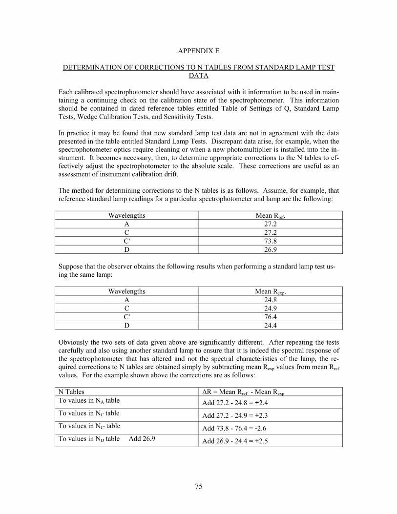
75

APPENDIX E

DETERMINATION OF CORRECTIONS TO N TABLES FROM STANDARD LAMP TEST DATA

Each calibrated spectrophotometer should have associated with it information to be used in main-taining a continuing check on the calibration state of the spectrophotometer. This information should be contained in dated reference tables entitled Table of Settings of Q, Standard Lamp Tests, Wedge Calibration Tests, and Sensitivity Tests. In practice it may be found that new standard lamp test data are not in agreement with the data presented in the table entitled Standard Lamp Tests. Discrepant data arise, for example, when the spectrophotometer optics require cleaning or when a new photomultiplier is installed into the in-strument. It becomes necessary, then, to determine appropriate corrections to the N tables to ef-fectively adjust the spectrophotometer to the absolute scale. These corrections are useful as an assessment of instrument calibration drift. The method for determining corrections to the N tables is as follows. Assume, for example, that reference standard lamp readings for a particular spectrophotometer and lamp are the following:

Wavelengths Mean Rref. A 27.2 C 27.2 C' 73.8 D 26.9

Suppose that the observer obtains the following results when performing a standard lamp test us-ing the same lamp:

Wavelengths Mean Rexp. A 24.8 C 24.9 C' 76.4 D 24.4

Obviously the two sets of data given above are significantly different. After repeating the tests carefully and also using another standard lamp to ensure that it is indeed the spectral response of the spectrophotometer that has altered and not the spectral characteristics of the lamp, the re-quired corrections to N tables are obtained simply by subtracting mean Rexp values from mean Rref values. For the example shown above the corrections are as follows: N Tables ΔR = Mean Rref - Mean Rexp To values in NA table Add 27.2 - 24.8 = +2.4 To values in NC table Add 27.2 - 24.9 = +2.3 To values in NC' table Add 73.8 - 76.4 = -2.6 To values in ND table Add 26.9 Add 26.9 - 24.4 = +2.5

76

Notice that the experimental A-wavelengths standard lamp reading, for example, is too low by 2.4 degrees. This means that when routine ozone measurements are made the RA and, hence, NA values will be too low by about 2.4 units. It is necessary to compensate for the change in the spectral response of the instrument by increasing NA values. The optical wedges of most spectrophotometers are designed in such a manner that a change of one R unit along the wedge corresponds very nearly to a change of one N unit along the wedge. Therefore, corrections to the N tables can be determined simply by comparing standard lamp test R-dial readings as has been done above; otherwise, corrections should be computed in terms of ΔN rather than ΔR. Ozone data that have been computed may occasionally have to be recomputed or corrected when an observer learns after performing a standard lamp test that the spectral response of his instru-ment has changed. The observer will have to use his discretion in deciding how much of the back data needs revision. For this reason it is important that standard lamp tests be performed at least once per month and that notes are kept regarding the occurrence of unusual events that may have a bearing on the spectral response of the spectrophotometer. The corrections affect the analysis to determine total ozone from double-pair measurements with the value (NA – ND) or (NC – ND). These values should be tracked, as the value of the (NA – ND) gives an indication of the change. A (NA – ND) value of ±0.7 is approximate ±1 percent change in total ozone. A value of this or large magnitude would suggest a calibration check against a stan-dard.

77

APPENDIX F

COMPUTATION OF COS Z AND μ FOR SUN AND MOON

In the time since the original publication of this handbook, there has been a great change in the basic calculations for the positions of the sun and the moon. The publication of the Astronomical Almanac by the U.S. Naval Observatory has been augmented by the publication of software ver-sions. The Multiyear Interactive Computer Almanac (MICA) is available from Willmann-Bell, Inc. (www.willbell.com). Version 2.0 covers the years 1800-2050, and is less that the cost of one year of the printed Almanac. This software greatly simplifies the calculation of the zenith angle and thus μ. 1. Physical Significance of μ, Z, and (HP). The dimensionless quantity, μ, is the ratio of the ozone layer path length traversed by a ray of light emanating from the sun or moon at the time of observation to the vertical path length. As illustrated in Figure F-1, μ is equal to the ratio of paths CD/AB. In practice, μ values are obtained from an equation which relates cosine (Z) and μ. The angle, Z, shown in the figure is referred to as the celestial body's zenith angle (or distance). At certain times during the day, Z may change rather quickly; hence, it is necessary to time observations to within ±5 seconds to preserve suffi-cient accuracy in the computed μ values.

Figure F-1. Graphical illustration of μ, Z and (HP)

78

Cosine (Z) values are obtained by solving the astronomical triangle equation

)sin(*)sin()cos(*)cos(*)cos()cos( φδφδθ +=Z (1) Notice in Figure F-1 that because of the great distance separating the sun and earth the zenith an-gle Z is very nearly equivalent to the angle Zo (the difference in angles is greatly exaggerated in the diagram). Hence, a solution of equation (1) yields cos(Z) at once. The moon, on the other hand, is relatively near the earth. As a result, Z is appreciably greater than Zo. The procedure here is to compute cos(Zo) from equation (1), then apply to it a parallax correction, Δcos(Zo), to obtain cos(Z). The parallax correction is obtained normally from a table which relates Δcos(Zo) to (HP), where the latter symbol denotes the moon's horizontal parallax obtained, e.g., from the Nautical Alma-nac, United States Naval Observatory, for the time of observation. The table has been computed from equation (4) given below, which is derived as follows. With reference to Figure F-1,

)cos(2)()(

22 o

o

ZrRrRrZRCosZCos

−+

−= (2)

where R is the separation of the earth and moon centres and r is the radius of the earth. By defi-nition

RrHP =)( [Radians] (3)

Dividing the numerator and denominator of the right hand side of equation (2) by R gives

)()(21)()(~)(

0ZCosHPHPZCosZCos

o

−

− rR >>

)()()(~ 2 oo ZSinHPZCos −

)()(~)( oo ZCosZCosZCos −Δ )()(~ 2 oZSinHP− (4)

The quantities θ, δ and φ in equation (1) are, respectively, the hour angle and declination of the luminescent celestial body, and the latitude of the observer's station. So that the observer com-prehend fully the significance of equation (1), a brief introduction to astronomical concepts is presented in Appendix H and Appendix I with which the reader is encouraged to become familiar before proceeding to the next section which deals with the method of computing cos(Z) and μ. 2. Calculation of Cos(Z) at Amundsen-Scott Station Amundsen-Scott station is located in Antarctica at latitude of nearly -90 degrees. Letting θ= -90° in equation (1) we obtain

cos(Zo)= - sin(δ). (5) Since cos(Zo) ~ cos(Z) for observations made on the sun, it is evident that Z can be determined at once from a knowledge of the sun's declination at any time: Zo ~ Z =90° + δ. (6)

79

μ is then simply obtained from a table relating cos(Z) and μ. For moon observations, the horizon-tal parallax has to be taken into account. Cos(Zo) is computed first: then the appropriate value of Δcos Z* is subtracted from cos(Zo) to give cos(Z).

Figure F-2. Illustration of Local Hour Angle at Sterling, Virginia

80

3. Example of MICA output. The output of the software package MICA is easily converted to a spreadsheet format. The ter-minology is slightly different. The Time UT1 is the within 1 second of the Official UTC. The Zenith Distance corresponds to Zenith Angle. Apparent Topocentric Positions include the paral-lax correction Δcos(Zo), considering the observation point to be on the surface of the earth. The value of μ (Section 7.1.4) than can easily found using interpolation to find the precise value of zenith angle.

Apparent Topocentric Positions Local Zenith and True North

Mauna Loa Observatory

Location: W155°34'42.0", N19°32'00.0", 3397m (Longitude referred to Greenwich meridian)

Date Time Zenith Azimuth Distance

(UT1) Distance (E of N) to Object h m s ° ° AU

… 7-Sep-06 19:00:00 50.49712 98.68736 1.0075855867-Sep-06 19:01:00 50.26428 98.80095 1.0075852767-Sep-06 19:02:00 50.03150 98.91517 1.0075849677-Sep-06 19:03:00 49.79881 99.03003 1.0075846587-Sep-06 19:04:00 49.56618 99.14555 1.0075843507-Sep-06 19:05:00 49.33363 99.26173 1.0075840427-Sep-06 19:06:00 49.10116 99.37859 1.0075837357-Sep-06 19:07:00 48.86877 99.49613 1.0075834287-Sep-06 19:08:00 48.63646 99.61437 1.0075831227-Sep-06 19:09:00 48.40423 99.73331 1.0075828167-Sep-06 19:10:00 48.17208 99.85298 1.0075825117-Sep-06 19:11:00 47.94002 99.97338 1.0075822067-Sep-06 19:12:00 47.70804 100.09452 1.0075819027-Sep-06 19:13:00 47.47615 100.21641 1.0075815987-Sep-06 19:14:00 47.24436 100.33907 1.0075812957-Sep-06 19:15:00 47.01265 100.46251 1.0075809927-Sep-06 19:16:00 46.78103 100.58674 1.0075806907-Sep-06 19:17:00 46.54951 100.71177 1.0075803897-Sep-06 19:18:00 46.31809 100.83762 1.0075800877-Sep-06 19:19:00 46.08676 100.96431 1.0075797877-Sep-06 19:20:00 45.85553 101.09183 1.007579487

… Table F-1. Example of MICA output for Mauna Loa Observatory, 07 September 2006. 4. Calculation of Z Times for Umkehr Observations Interpolation can be used in the output of MICA to determine the precise time of a zenith angle. 5. Cos(Z )Determinations by Computer

81

Yallop (1977) and Sinclair and Yallop (1977) have devised computer algorithms for computing solar hour angles and declinations corresponding to a precision in sun positions of 1' of arc. The following algorithms are based on a machine algorithm for processing calendar dates by Fliegel and Flandern (1968), and provide information of adequate precision for the processing of total ozone data for several centuries around 1980.

POSITION OF THE SUN TO 1' OF ARC PRECISION a) Definitions

Julian day number = number of days elapsed since 12h UT on BC4713 Julian date = Julian day number followed by the fraction of a day elapsed since the preceding

noon.

b) Variables D = number of days from 1900.0 (Julian date 2415020.0) T = number of Julian centuries from 1900.0 = D/36525 L = mean longitude of sun in degrees E = equation of time (in seconds of time) ε = obliquity of the ecliptic α = right ascension of sun (apparent) in degrees δ = declination of sun (apparent) in degrees GHA = Greenwich hour angle of sun (in degrees) UT = Universal time which is equivalent to GMT in this context (in degrees)

c) Formulae

2415020_ −= dateJulianD

36525DT = TL *769.3000697.279 +=

)cos(*)*2063.0*7.35.432()sin(*)*0144.0*23.140.93( 22 LTTLTTE −−−−+−= )*2cos(*)*28.04.1()*2sin(*)*0096.0*81.09.596( 2 LTLTT +−−−+

)*3cos(*)*0103.0*21.05.19()*3sin(*)*60.08.3( 2 LTTLT −−+++ )*4sin(*)*03.08.12( LT−−

T*00027.043382.0)tan( −=ε 240EL −=α

)sin(*)tan()tan( αεδ = 180240++= EUTGHA

d) Worked Example Find GHA and declination of the sun on 1976 August 8 at 6h UT

75.27978=D 7660164.0=T

°= 877.136L 4.335−=E (in seconds of time) =-= -1.397°

82

433613.0)( =εTan '4.16138274.138 °=°=α

'9.516098.16 °=°=δ '2.36268603.268 °=°=GHA GHA

Yallop, B.D., Position of the sun to 1' of arc precision, H.M. Nautical Almanac Office, Royal

Greenwich Observatory, Herstmonceux Castle, Hailsham, Sussex BN27 1RP, 1977. CALCULATION OF THE TIME-INTERVAL FROM THE BEGINNING OF 1900

i. Definitions I = year of date J = month (January = 1, February = 2, etc) K = day of month UT = Universal time in hours D = time elapsed in days, since 1900 Jan 0d at Greenwich noon = JD2415020.0 to date and time required The formula given below is intended for a calculator which has a function called INT which removes the fractional part of a number. The formula has been derived from an expression written in the computer language of FORTRAN and was first given by H F Fliegal and T C van Flandern in the Journal of the Association for Computing Machinery, (1968), 11, 659.

ii. Formulae Compute

12)14( −= JA )(AINTB =

4)4800(*1461 BIC ++= )(CINTU =

12)*122(*367 BJE −−= )(EINTV =

100)4900( BIG ++= 4)(*3 GINTH =

245.2447095)(

UTWVUKDHINTW

++++−=−=

Where INT(X) means take the integer part of X

83

iii. Worked Example

Find D on 1976 Feb 3 at 6h UT

1976=I 2=J 3=K 6=UT 1−=A 1−=B 75.2474568=C

2474568=U 0.367=E 367=V 75.68=G 51=H 51−=W

75.27791=D

84

APPENDIX G

INTRODUCTION TO PRINCIPLES OF ASTRONOMY

1. Celestial Sphere The celestial sphere is an imaginary globe of infinite radius at whose center is located the earth. In the "shell" of the sphere are embedded the stars and the sun. The earth is imagined to be fixed, and the celestial sphere to be rotating from east to west, its axis being the prolongation of that of the earth. Thus, to the naked eye the pole star remains nearly stationary. The portion of the celestial sphere seen by the observer is the hemisphere above the plane of his own horizon. A vertical line at the position of the observer coincides with the plumb line and is normal to the observer's horizon plane. The point in intersection of the vertical line and celestial sphere boundary is the zenith. A corresponding point in the opposite hemisphere is called the observer's nadir. The celestial equator is the great circle formed by the intersection of the earth's equatorial plane with the surface of the celestial sphere. The celestial poles are the points where the extended earth's axis pierces the celestial sphere. 2. Observer's Position on Earth The position of any point on the surface of a sphere may be fixed by angular measure-ment from two planes of reference at right angles to each other passing through the centre of the sphere; these measurements are called the spherical coordinates of that point. The spherical coordinates of any station on the earth are designated as the latitude and longitude of the station. The latitude of a station is defined as the angular distance of the station below or above the equa-tor. When the station is above the equator, the latitude is north and its sign is positive, e.g., +47° or 47°. When below the equator, the latitude of the station is south and its sign is negative. A parallel is the line joining all points which are at the same latitude, i.e., parallel to the equatorial circle. A meridian circle is any circle on the surface of the earth passing through both the north and south poles. The longitude of a station is defined as the angular distance measured along the arc of the equator between a primary meridian, which is a reference meridian, and the meridian circle passing through the station. The primary meridian most generally used is that of Greenwich, England. Longitudes are expressed either in degrees or arc or in hours of time (15° = 1 hr.) and are meas-ured either east or west of the Greenwich meridian. 3. Position of a Celestial Body Two systems of coordinates are commonly used to describe the position of a celestial body. If it is required only to specify a star's position on the celestial sphere, the right ascension system of coordinates is employed. When the position of a star with respect to the meridian through a given

85

station on the surface of the earth is to be determined, the hour angle system of coordinates is used.

Figure H-1 Celestial Hemisphere (a) Right Ascension Coordinate System. In Figure H-1, S is a celestial body on the celestial hemisphere whose position is to be fixed by spherical coordinates. The earth is located at the centre, O, of the sphere with its axis in the direction of OP. Hour circles on the celestial sphere compare with the meridian circles or meridians of longitude of the earth. In the figure, PSU is an hour circle arc. Parallels of declination of the celestial sphere compare with the parallels of latitude of the earth. The equinoctial colure of the celestial sphere passes through the vernal equinox, V, an imaginary point among the stars where the sun apparently crosses the equator from south to north on March 21 (approximately) of each year. The E.C. compares with the prime meridian through Greenwich. Right ascension of the sun or any star (comparable to the longitude of a station on earth) is the angular distance, α, measured along the celestial equator between the vernal equinox and the hour circle through the body. Right ascensions are measured eastward from the vernal equinox and may be expressed in degrees of arc (0° to 360°) or in hours of time (0h to 24h). Declination of any celestial body is the angular distance, δ, of the body above or below the celes-tial equator. It is comparable with the latitude of the station on earth. If the body is above the

86

equator its declination is said to be north and is considered as positive; if it is below the equator its declination is said to be south and is considered negative. Declinations are expressed in de-grees and cannot exceed 90° in magnitude. Polar distance of any celestial body is = 90° - δ with due regard to the sign of the declination. For the present purpose the vernal equinox is assumed to be a fixed point on the celestial equator. However, the coordinates of celestial bodies with respect to the celestial equator and the equinoc-tial colure change slightly with the passage of time. The fixed stars, or those outside the solar system, alter their positions in the celestial sphere only slightly from month to month and from year to year, the annual change being less than a minute of arc in either right ascension or decli-nation. These variations result from precession or the slow change in the direction of the earth's axis caused by attraction of the sun, moon and planets, and nutation or small inequalities in the motion of precession. Proper motion of stars also occurs, that is, stars actually move very slightly with respect to the celestial sphere as time goes on. Furthermore, aberration, or an apparent change in position of heavenly bodies occurs, with a period of one year, because of the combined effect of the motion of light and motion of the observer fixed on the moving earth. Finally, the angle subtended by lines drawn from any star to the earth and sun changes continuously as the earth makes its annual circuit around the sun. As a result, the positions of the stars seem to change on the celestial sphere due to parallax. As the earth actually travels around the sun but not the stars, (see Figure H-2) the sun appears to move more slowly than the stars, making in 1 year 365 apparent revolutions (approx.) while the stars make 366 apparent revolutions (approx.); thus, the sun apparently makes a complete circuit of the heavens once each year, a new cycle beginning every March 21. Furthermore, as the axis of rotation of the earth is not normal to the plane of the earth's orbit, the path apparently traced by the sun among the stars on the celestial sphere, called the ecliptic, is a continuous curved line; each year the sun crosses the equator northward on March 21, and reaches a maximum positive declination (about 23.5° N) on June 21.

Figure H-2. Relative positions of the earth and the sun during the year

(b) The Hour Angle Coordinate System. In Figure H-1, let the plane of the hour circle MNPN'M' coincide at the time of observation with the plane of the observer's meridian circle, and let S be some heavenly body whose position with respect to the observer's meridian and the equator MM'UV it is desired to establish. The spherical coordinates of the star are given by (1) the angu-

87

lar distance of the star above or below the equator, which in the figure is given by the arc US, defined previously as the declination, and (2) the angular distance measured along the equator between the meridian and the hour circle through the star. When this measurement is from east to west it is called an hour angle. The hour angle of any celestial body may then be defined as the angular distance measured westward along the equator from the meridian of reference to the hour circle through the body. Hour angles are expressed either in hours of time or in degrees of arc. In the figure, the hour angle is more than 12h or more than 180°. When no qualification is stated, it is understood that an hour angle is measured from the upper branch of the meridian, that is, the branch above the station or above the observer's head. Sometimes the hour angles of stars east of the observer's meridian are reckoned from the upper branch of the meridian rather than westward. An hour angle expressed in this way is preceded by a minus sign. 4. Equator Systems Compared The system of coordinates described in article (b) is seen to be similar, to that described in article (a) with this difference, that in the hour angle system, the angular distance along the equator is measured (westward) from a fixed meridian, whereas in the right ascension system the angular distance along the equator is measured (eastward) from the vernal equinox, which is a point on the celestial equator that rotates with the celestial sphere. Thus, although right ascensions of fixed stars have annual variations of but a few seconds, hour angles of the stars change as rapidly as the celestial sphere apparently rotates (24h or 360° for each 23h 56s of our civil time), and hour angles of the sun change approximately 24h or 360° for each 24h of our civil time. The two systems are called equatorial systems of coordinates, since in each case the primary plane of reference is the celestial equator. The declination, δ, is the same in both systems. 5. The Astronomical Triangle

Figure H-3. The Astronomical Triangle

88

In Figure H-3, the celestial sphere is pictured once again. The earth is imagined to be located at the center of the sphere with its polar axis in the direction P'P. The observer's meridian plane lies in the plane of the great circle M'Q'ZPMQP' and the star S is in a position east of the meridian and above the celestial equator. The place of observation is as-sumed to be north of the equator at a latitude φ as shown by the angle between the equatorial plane and the observer's zenith plumb line. The hour angle, θ, is measured from the upper branch of the meridian (360° - θ is shown in the figure). The declination, δ, is also shown. The colatitude (90°- φ), the zenith distance (Z), and the polar distance (90° - delta) define a spherical triangle the vertices of which are the pole P, the zenith Z, and the celestial body S. This triangle is called the astronomical triangle. The determination of the relationship between theta and Z, 90° - φ and 90° - δ of the astronomical triangle is a problem in spherical trigonometry which is dealt with in many elementary mathe-matical texts. It is sufficient to quote the result here:

)sin(*)sin()cos()cos(*)cos()cos( φδφδθ +=Z This is the equation that must be solved for cos(Z) to obtain μ.

89

APPENDIX H

CONCEPT OF TIME

1. Solar and Sidereal Time As the earth rotates about its axis in its travel through space, all celestial bodies apparently rotate about the earth (or about its axis) from east to west. Since the earth in its orbit travels about the sun but not about the fixed stars, which are far outside its orbit, once each year the sun apparently encircles the celestial sphere along a path called the ecliptic, which twice cuts the celestial equa-tor during this interval. The point among the stars where the sun in its apparent travel northward cuts the celestial equator on March 21 of each year is called the vernal equinox. The sun travels rapidly along the ecliptic in a direction opposite to that of the rotation of the celestial sphere. Because the sun is apparently traveling from west to east among the stars, whereas the rotation of the celestial sphere about the earth is apparently from east to west, the angular velocity of the sun about the axis of the celestial sphere is less than that of the fixed stars or the vernal equinox. At a given meridian the hour angle of the sun and of the vernal equinox will agree at some instant on March 21, but thereafter it will be less for the sun than for the vernal equinox. Six months later, on September 22, when the sun has covered one-half of its annual journey, the hour angle of the sun will be 180° or 12h less than that of the vernal equinox; and one year later the angle of the sun will be 360° or 24h less than that of the vernal equinox, and hence hour angles will agree. In the course of a tropical year, as measured by the time taken by the sun apparently to make a complete circuit of the ecliptic, there actually occur 366.2422 rotations of the earth, or apparently a like number of revolutions of the vernal equinox about the earth. For reasons explained, the sun during this interval will have traveled through a total hour angle 360° or 24h less than that trav-ersed by the vernal equinox; hence, during a tropical year the sun apparently revolves about the earth 365.2422 times. Solar day is the unit of time with which we are all familiar. It is the interval of time occupied by one apparent revolution of the sun about the earth. Sidereal day is the unit of time occupied by one apparent revolution of the vernal equinox. 366.2422 sidereal days = 365.2422 solar days. The sidereal day is shorter than the solar day. When any celestial body apparently crosses the upper branch of a meridian, it is said to be at up-per transit; when any celestial body crosses the lower branch of the meridian, it is said to be at lower transit. Beginning of a sidereal day at a given place occurs at the instant the vernal equinox is at upper transit. Beginning of a solar day, or the civil day, occurs at the instant of lower transit of the sun (mid-night). 2. True and Mean Suns Because of the elliptical shape of the earth's orbit, the apparent angular velocity of the sun that we see, or the true sun, is not constant; hence, the days as indicated by the apparent travel of the true sun about the earth are not of uniform length as measured by a mechanical clock. To make our

90

solar day of uniform length, astronomers have invented the mean sun, a fictitious body which is imagined to move at a uniform rate along the celestial equator, making a complete circuit from west to east in one year. The time interval as measured by one apparent revolution of the true sun about the earth is called an apparent solar day. The time interval as measured by one daily revolution of the mean sun is called the mean solar day, which is the same as the civil day. 3. Apparent (True) Solar Time The "Nautical Almanac" considers the apparent solar day at any place as the time interval be-tween two successive lower transits of the true (apparent) sun for the meridian of that place. The solar day therefore begins at midnight and the apparent solar time at any place is given by the hour angle of the true sun plus 12h. Thus, if the hour angle of the sun is 45° or 3h at a given place and at a given instant, then the apparent solar time for the place is 3h+12h=15h. Apparent time has the same meaning as apparent solar time. Local apparent time is that for the meridian of the observer. Apparent time for any other meridian is designated by name, for exam-ple, Greenwich apparent time.. In the local apparent time the sun peaks its daily journey in the South and exactly at 12:00. 4. Civil (Mean Solar) Time The "Nautical Almanac" considers the mean solar day at any place to be the time interval be-tween two successive lower transits of the mean sun for the meridian of that place. The mean solar day, therefore, also begins at midnight, and the mean solar time is given by the hour angle of the mean sun plus 12h. Thus, if the hour angle of the mean sun is -15° = 1h, the mean solar time is 11h. Civil time is the same as mean solar time or mean time. Local civil time is that for the meridian of the observer. Civil time for any other meridian is designated by name, for exam-ple, Greenwich civil time, or Greenwich Mean Time. 5. Equation of Time When the apparent (true) sun is (ahead of/behind) the mean sun, apparent time is (faster/slower) than mean civil time. The difference between apparent and civil time at any instant is called the equation of time. It is used to convert civil time at any instant to apparent time. In the "Nautical Almanac" the equation of time is given for each day for the hours 00 and 12 Greenwich civil time. The Greenwich civil time at which the true sun crosses the Greenwich me-ridian is also given. This information is useful in establishing whether the true sun is ahead of or behind the mean sun. 6. Sidereal Time The sidereal time at any place is the hour angle of the vernal equinox at that place; and the begin-ning of the sidereal day, occurring when the vernal equinox crosses the upper branch of the me-ridian, is called sidereal noon. 7. Relationship Between Longitude and Time

91

At any instant, the difference in local time between two places, whether the time under considera-tion is sidereal, mean, or apparent solar, is equal to the difference in longitude between the two places expressed in hours. The 1-hour difference corresponds to 150 in longitude. 8. Standard Time To eliminate the confusion in industry attendant upon the use of local time by the public, the United States is divided into belts, each of which occupies a width of approximately 15° 1h of longitude. In each belt the clocks that control civil affairs all keep the same time, called Standard Time, which is the local civil time for a meridian near the center of the belt. The time in any belt is a whole number of hours slower than Greenwich civil time, as follows:

Standard Time Hours Slower than

Greenwich Civil Time Central Meridian Atlantic 4 60° W Eastern 5 75° W Central 6 90° W

Mountain 7 105° W Pacific 8 120° W

The exact boundaries of the time belts are irregular and can be determined only from a map. Correct standard time can be obtained either from a clock known to be closely regulated, radio signals, a GPS receiver or an internet time service. In certain localities, daylight saving time is used during the summer months. Daylight saving time is 1h faster than standard time.