operational domain theory and topology of sequential functional

The University of BirminghamSchool of Computer Science

Operational Domain Theory andTopology of

Sequential Functional Languages

Weng Kin Ho

Dr. Martın EscardoSupervisor

Dr. Alex SimpsonExternal Examiner

Dr. Paul Blain LevyInternal Examiner

A dissertation submitted for the degree ofDOCTOR OF PHILOSOPHY

inComputer Science

The University of BirminghamSubmitted August 18, 2006Defended October 4, 2006

Declaration

The results reported in Part III consist of joint work with Martın Escardo [14].All the other results reported in this thesis are due to the author, except forbackground results, which are clearly stated as such. Some of the results inPart IV have already appeared as [28].

Note This version of the thesis, produced on October 31, 2006, is theresult of completing all the minor modifications as suggested by both theexaminers in the viva report (Ref: CLM/AC/497773).

i

Abstract

We develop an operational domain theory to reason about programsin sequential functional languages. The central idea is to export domain-theoretic techniques of the Scott denotational semantics directly to the studyof contextual pre-order and equivalence. We investigate to what extent thiscan be done for two deterministic functional programming languages: PCF(Programming-language for Computable Functionals) and FPC (Fixed PointCalculus).

Traditionally, domain theory and topology in programming languageshave been applied to manufacture and study denotational models, for in-stance, the Scott model of PCF. For a sequential language like this, it iswell-known that the match of the model with the operational semantics isimprecise: computational adequacy holds but full abstraction fails.

One of the main achievements is a reconciliation of a good deal of domaintheory and topology with sequential computation. This is accomplished byside-stepping denotational semantics and reformulating domain-theoretic andtopological notions directly in terms of programming concepts, interpretedin an operational way. Regarding operational domain theory, we introduceoperational finiteness. The upshot is the SFP theorem: Every PCF typehas an SFP structure. In particular, the set of finite elements of each typeforms a basis. Regarding operational topology, we work with an operationalnotion of compactness. The elegance of the theory lies not only in the inter-play of these two notions but also in the reasoning principles that emerge.For instance, we show that total programs with values on certain types areuniformly continuous on compact sets of total elements. We apply this andother conclusions to prove the correctness of non-trivial PCF programs thatmanipulate infinite data.

For FPC, an operational domain theory is developed for treating recursivetypes. The principal approach taken here deviates from classical domain the-ory in that we do not produce recursive types via inverse limit constructions -we have it for free by working directly with the operational semantics of FPC.The important step taken in this work is to extend type expressions to legiti-mate n-ary functors on suitable ‘syntactic’ categories. To achieve this, we relyon operational versions of the Plotkin’s uniformity principle and the minimal

ii

invariance property. This provides a basis for us to introduce the operationalnotion of algebraic compactness. We then establish algebraic compactnessresults in this operational setting. In addition, a “pre-deflationary” structureis derived on closed FPC types and this is used to generalise the “GenericApproximation Lemma” recently developed by Hutton and Gibbons. Thislemma provided a powerful tool for proving program equivalence by simpleinductions, where previously various other more complex methods had beenemployed.

iii

For my beloved family“As for me and my house we will serve the Lord.” (Joshua 24:15)

iv

Acknowledgements

I thank God for giving me this once-in-a-lifetime opportunity to pursuea PhD. While in Singapore, a joint work with my M.Sc. supervisor, Dong-sheng Zhao, in the Nanyang Technological University regarding Scott-closedsets saw a small breakthrough. Things just somehow started to unfold in myfavour, beginning with a rather fortuitous acquaintance with my PhD su-pervisor, Martın Escardo. In our communication, we were amazed that mywork [27] on characterising the Scott-closed set lattices was closely relatedto Martın’s work [12] on injective locales over perfect sublocale embeddings.Subsequently, I received the kind invitation from Martın Escardo and AchimJung to present my findings in the workshop Domains VI in Birmingham,September 16-19, 2002. Besides meeting the domain theory and program-ming language semantics community, I received an unexpected opportunityto be interviewed by Peter Hancox, the Admissions Tutor. In 2003, I wasawarded an International Research Studentship from the School of Computer(The University of Birmingham), which made this work possible. I am grate-ful to the School of Computer Science, The University of Birmingham, andespecially to Martın Escardo, Achim Jung and Peter Hancox.

My three years of study in Birmingham proved to be a rich experience.I benefitted from a rich resource of research material and expert advice. Iam extremely grateful to my supervisor, Martın Escardo, for all his help andencouragement. This was especially the case during my first year of studyin which I must put in more effort to understand the “computer science”component of my research. I benefitted from the weekly meetings with him,in which I was inspired and intrigued by his vast knowledge and ingeniousideas. His deep insights (especially in his work [13]) so very much motivatedand shaped the entire course of my research that he deserves most of thecredit for my work. I am particularly thankful for the opportunity of ajoint work (Escardo & Ho [14]) with him, in which we had many fruitfuldiscussions. I shall always remain in intellectual debt with Martın becausehe has taught me how to do research.

I want to extend my special gratitude to the School’s research group:Mathematical Foundations of Computer Science. They provided a ready au-dience (together with constructive criticisms) to whom I shared my research

v

findings. In particular, I thank Paul Blain Levy for giving me opportunitiesin the informal lunch talks where I was allowed to rehearse for more formalones. Regarding external seminars, I am also thankful to Dongsheng Zhao(Nanyang Technological University, Singapore) and Alexander Kurz (Uni-versity of Leicester, UK) for inviting me to speak in several occasions aboutmy work. In particular, I am very encouraged by Alexander Kurz and NeilGhani (University of Leicester, UK) when they expressed enthusiasm in mywork.

My study was enriched by the various research conferences which I at-tended. I would like to acknowledge the Research Committee in funding mytrips to academic events, such as MGS 2003 and 2004, LICS 2005 and MFPS2006. In these events, not only did I learn about the works of others butalso meet several excellent researchers from all over the world. In particular,I got acquainted with Andrew Pitts and Thomas Streicher who later offeredme very timely and useful advice. Andrew Pitts patiently entertained myseries of emails seeking clarification on the operational machineries whichhe developed in Pitts [41]. Following his suggestion, I was able to developthe operational toolkit for arguing about program equivalence for FPC (cf.Part II). Thomas Streicher went the extra mile in offering expert advice as Ifixed a gap in Alexander Rohr’s reasoning regarding the minimal invarianceof syntactic functors (cf. Rohr [47]). This resulted in the establishment ofoperational algebraic compactness with respect to the class of syntactic func-tors. I am grateful to both of them for patiently and carefully reading my(manuscript) preprint of Ho [28]. Regarding the Midland Graduate School, Iwas most inspired by a series of lectures given by Achim Jung on denotationalsemantics in MGS 2004.

During these three years, I have had many invaluable discussions withmany researchers such as Steve Vickers (topology via logic), Paul Levy (de-notational semantics) and Achim Jung (domain theory, especially Chapter5 of [3]). My fellow colleagues, including Jose Raymundo Marcial-Romero,Thomas Anberree and Mohamed El-Zawawy, often lent me their ears. Wehad a wonderful time together in our reading group on the domain-theorybible [21]. I am grateful to Thomas Anberree for proof-reading some parts ofthis thesis. I want to especially thank Martın for carefully having proof-readthe entire thesis. All the remaining mistakes are, of course, due to myself.

All the commutative diagrams in this thesis were produced with PaulTaylor’s commutative diagrams package.

Special thanks goes to my wife, Hwee Hoong, and my (now four-yearold) son, Samuel, for supporting me in every possible way throughout mystudy in the UK. Each time I get back from work, their warm welcome andhugs meant an entire world to me. Also I would like to thank the unflagging

vi

support of my father and my parents-in-law for my overseas studies despitetheir old age.

Finally, I thank my family-in-Christ from the Birmingham Chinese MethodistChurch (UK) and the Aldersgate Methodist Church (Singapore) for givingme the spiritual support and guidance during these three years in the UK.

vii

Contents

1 Introduction 11.1 Brief summary of contributions . . . . . . . . . . . . . . . . . 3

1.1.1 Operational domain theory and topology for PCF . . . 31.1.2 Operational domain theory for FPC . . . . . . . . . . . 5

1.2 Additional contributions . . . . . . . . . . . . . . . . . . . . . 61.3 Background . . . . . . . . . . . . . . . . . . . . . . . . . . . . 61.4 Organisation . . . . . . . . . . . . . . . . . . . . . . . . . . . . 7

I Background 8

2 Prerequisites 102.1 Domain theory . . . . . . . . . . . . . . . . . . . . . . . . . . 10

2.1.1 Directed complete posets . . . . . . . . . . . . . . . . . 102.1.2 Scott topology . . . . . . . . . . . . . . . . . . . . . . . 112.1.3 Dcpos and least fixed-points . . . . . . . . . . . . . . . 112.1.4 Complete lattices and the Tarski-Knaster fixed-point

theorem . . . . . . . . . . . . . . . . . . . . . . . . . . 122.1.5 Domains and algebraic domains . . . . . . . . . . . . . 12

2.2 Essential categorical notions . . . . . . . . . . . . . . . . . . . 152.2.1 Limits and colimits . . . . . . . . . . . . . . . . . . . . 152.2.2 Algebras and coalgebras . . . . . . . . . . . . . . . . . 152.2.3 Adjunctions . . . . . . . . . . . . . . . . . . . . . . . . 162.2.4 Involutory and locally involutory categories . . . . . . 17

2.3 Recursive domain equations . . . . . . . . . . . . . . . . . . . 192.3.1 Construction of solutions . . . . . . . . . . . . . . . . . 202.3.2 Canonicity . . . . . . . . . . . . . . . . . . . . . . . . . 212.3.3 Mixed variance . . . . . . . . . . . . . . . . . . . . . . 22

2.4 Algebraic completeness and compactness . . . . . . . . . . . . 242.4.1 Parametrised algebraic completeness . . . . . . . . . . 242.4.2 Parametrised algebraic compactness . . . . . . . . . . . 25

viii

2.4.3 The Product Theorem . . . . . . . . . . . . . . . . . . 25

3 The programming language PCF 273.1 The language PCF . . . . . . . . . . . . . . . . . . . . . . . . 273.2 Operational semantics . . . . . . . . . . . . . . . . . . . . . . 303.3 Extensions of PCF . . . . . . . . . . . . . . . . . . . . . . . . 32

3.3.1 Oracles . . . . . . . . . . . . . . . . . . . . . . . . . . . 323.3.2 Parallel features . . . . . . . . . . . . . . . . . . . . . . 323.3.3 Existential quantifier . . . . . . . . . . . . . . . . . . . 333.3.4 PCF++

Ω . . . . . . . . . . . . . . . . . . . . . . . . . . . 343.4 PCF context . . . . . . . . . . . . . . . . . . . . . . . . . . . . 343.5 Typed contexts . . . . . . . . . . . . . . . . . . . . . . . . . . 353.6 Contextual equivalence and preorder . . . . . . . . . . . . . . 363.7 Extensionality and monotonicity . . . . . . . . . . . . . . . . . 37

4 The programming language FPC 394.1 The language FPC . . . . . . . . . . . . . . . . . . . . . . . . 394.2 Operational semantics . . . . . . . . . . . . . . . . . . . . . . 414.3 Fixed point operator . . . . . . . . . . . . . . . . . . . . . . . 424.4 Some notations . . . . . . . . . . . . . . . . . . . . . . . . . . 424.5 FPC contexts . . . . . . . . . . . . . . . . . . . . . . . . . . . 444.6 Denotational semantics . . . . . . . . . . . . . . . . . . . . . . 46

4.6.1 Interpretation of types . . . . . . . . . . . . . . . . . . 464.6.2 Interpretation of terms . . . . . . . . . . . . . . . . . . 474.6.3 Soundness and computational adequacy . . . . . . . . 47

5 Synthetic topology 495.1 Continuous maps . . . . . . . . . . . . . . . . . . . . . . . . . 495.2 Open and closed subsets . . . . . . . . . . . . . . . . . . . . . 505.3 Closure of open sets under set-union . . . . . . . . . . . . . . 515.4 Subspace . . . . . . . . . . . . . . . . . . . . . . . . . . . . . . 525.5 Separation axioms . . . . . . . . . . . . . . . . . . . . . . . . 535.6 Specialisation order . . . . . . . . . . . . . . . . . . . . . . . . 555.7 Compact sets . . . . . . . . . . . . . . . . . . . . . . . . . . . 565.8 Properties of compact sets . . . . . . . . . . . . . . . . . . . . 57

II Operational Toolkit 59

6 Contextual equivalence and PCF bisimilarity 616.1 Bisimulation and bisimilarity . . . . . . . . . . . . . . . . . . . 61

ix

6.2 Co-induction principle . . . . . . . . . . . . . . . . . . . . . . 636.3 Operational extensionality theorem . . . . . . . . . . . . . . . 646.4 Kleene preorder and equivalence . . . . . . . . . . . . . . . . . 646.5 Elements of ordinal type . . . . . . . . . . . . . . . . . . . . . 666.6 Rational chains . . . . . . . . . . . . . . . . . . . . . . . . . . 68

7 Contextual equivalence and FPC bisimilarity 697.1 Properties of FPC contextual equivalence . . . . . . . . . . . . 69

7.1.1 Inequational logic . . . . . . . . . . . . . . . . . . . . . 697.1.2 β-equalities . . . . . . . . . . . . . . . . . . . . . . . . 707.1.3 Extensionality properties . . . . . . . . . . . . . . . . . 717.1.4 η-equalities . . . . . . . . . . . . . . . . . . . . . . . . 727.1.5 Unfolding recursive terms . . . . . . . . . . . . . . . . 727.1.6 Syntactic bottom . . . . . . . . . . . . . . . . . . . . . 737.1.7 Rational-chain completeness and continuity . . . . . . 73

7.2 FPC similarity and bisimilarity . . . . . . . . . . . . . . . . . 747.3 Co-induction principle . . . . . . . . . . . . . . . . . . . . . . 767.4 Operational extensionality theorem . . . . . . . . . . . . . . . 787.5 Kleene preorder and equivalence . . . . . . . . . . . . . . . . . 797.6 Continuity of evaluation . . . . . . . . . . . . . . . . . . . . . 81

8 Operational extensionality theorem 928.1 Precongruence and congruence . . . . . . . . . . . . . . . . . . 938.2 An auxiliary relation . . . . . . . . . . . . . . . . . . . . . . . 968.3 Open similarity is an FPC precongruence . . . . . . . . . . . . 998.4 Contextual preorder is an FPC simulation . . . . . . . . . . . 1008.5 Appendix . . . . . . . . . . . . . . . . . . . . . . . . . . . . . 104

III Operational Domain Theory for PCF 118

9 Rational chains and rational topology 1209.1 Rationale for rational chains . . . . . . . . . . . . . . . . . . . 1209.2 Rational continuity . . . . . . . . . . . . . . . . . . . . . . . . 1219.3 Rational topology . . . . . . . . . . . . . . . . . . . . . . . . . 122

10 Finiteness and SFP-structure 12410.1 Finiteness . . . . . . . . . . . . . . . . . . . . . . . . . . . . . 12410.2 Rational algebraicity . . . . . . . . . . . . . . . . . . . . . . . 12510.3 Deflation and SFP structure . . . . . . . . . . . . . . . . . . . 12610.4 A continuity principle . . . . . . . . . . . . . . . . . . . . . . . 134

x

10.5 An ultrametric on PCF . . . . . . . . . . . . . . . . . . . . . . 13610.6 Dense sets . . . . . . . . . . . . . . . . . . . . . . . . . . . . . 139

11 Compactness revisited 14211.1 Rational Heine-Borel property . . . . . . . . . . . . . . . . . . 14211.2 Saturation . . . . . . . . . . . . . . . . . . . . . . . . . . . . . 14311.3 Compact open sets . . . . . . . . . . . . . . . . . . . . . . . . 14511.4 Compact saturated sets . . . . . . . . . . . . . . . . . . . . . . 14511.5 Intersections of compact saturated sets . . . . . . . . . . . . . 14611.6 A non-trivial example of a compact set . . . . . . . . . . . . . 14711.7 Uniform-continuity principles . . . . . . . . . . . . . . . . . . 149

12 Sample applications 15112.1 Data language: an extension with oracles . . . . . . . . . . . . 15112.2 Equivalence with respect to ground D-contexts . . . . . . . . . 15212.3 The Cantor space . . . . . . . . . . . . . . . . . . . . . . . . . 15312.4 Universal quantification for boolean-valued predicates . . . . . 15512.5 The supremum of the values of a function . . . . . . . . . . . 156

IV Operational Domain Theory for FPC 161

13 FPC considered as a category 16313.1 The category of FPC types . . . . . . . . . . . . . . . . . . . . 16313.2 Basic functors . . . . . . . . . . . . . . . . . . . . . . . . . . . 16413.3 Realisable functors . . . . . . . . . . . . . . . . . . . . . . . . 170

14 Operational algebraic compactness 17914.1 Operational algebraic compactness . . . . . . . . . . . . . . . 18014.2 Alternative choice of category . . . . . . . . . . . . . . . . . . 18314.3 On the choice of categorical frameworks . . . . . . . . . . . . . 194

15 The Generic Approximation Lemma 20115.1 Standard FPC pre-deflations . . . . . . . . . . . . . . . . . . . 20115.2 The Generic Approximation Lemma . . . . . . . . . . . . . . . 20215.3 Sample applications . . . . . . . . . . . . . . . . . . . . . . . . 203

15.3.1 List type and some related notations . . . . . . . . . . 20315.3.2 The map-iterate property . . . . . . . . . . . . . . . . 20515.3.3 Zipping two natural number lists . . . . . . . . . . . . 20815.3.4 The ‘take’ lemma . . . . . . . . . . . . . . . . . . . . . 21215.3.5 The filter-map property . . . . . . . . . . . . . . . . . 214

xi

V Conclusion 218

16 Open problems and future work 22016.1 An operational proof of the minimal invariance property . . . 220

16.1.1 Functoriality . . . . . . . . . . . . . . . . . . . . . . . 22016.1.2 Pre-deflations revisited . . . . . . . . . . . . . . . . . . 22116.1.3 Compilation relation . . . . . . . . . . . . . . . . . . . 22316.1.4 Compilation of a context . . . . . . . . . . . . . . . . . 22516.1.5 A crucial lemma . . . . . . . . . . . . . . . . . . . . . 22716.1.6 Incomplete proof of functoriality . . . . . . . . . . . . . 230

16.2 SFP structure on FPC closed types . . . . . . . . . . . . . . . 23116.3 Relational properties of recursive types . . . . . . . . . . . . . 23216.4 Non-determinism and probability . . . . . . . . . . . . . . . . 232

17 Summary of work done 23417.1 Operational domain theory for PCF . . . . . . . . . . . . . . . 234

17.1.1 Rational completeness . . . . . . . . . . . . . . . . . . 23417.1.2 Operational topology . . . . . . . . . . . . . . . . . . . 23517.1.3 Operational finiteness . . . . . . . . . . . . . . . . . . . 23517.1.4 Data language . . . . . . . . . . . . . . . . . . . . . . . 23617.1.5 Program correctness . . . . . . . . . . . . . . . . . . . 236

17.2 Operational domain theory for FPC . . . . . . . . . . . . . . . 23617.2.1 Type expressions as functors . . . . . . . . . . . . . . . 23617.2.2 Operational algebraic compactness . . . . . . . . . . . 23717.2.3 Generic approximation lemma . . . . . . . . . . . . . . 237

A Improvements to Ho [28] 238

xii

List of Figures

3.1 PCF syntax . . . . . . . . . . . . . . . . . . . . . . . . . . . . 293.2 Rules for type assignment in PCF . . . . . . . . . . . . . . . . 303.3 Rules for evaluating PCF terms . . . . . . . . . . . . . . . . . 31

4.1 FPC syntax . . . . . . . . . . . . . . . . . . . . . . . . . . . . 404.2 Rules for type assignments in FPC . . . . . . . . . . . . . . . 414.3 Rules for evaluating FPC terms . . . . . . . . . . . . . . . . . 424.4 FPC contexts . . . . . . . . . . . . . . . . . . . . . . . . . . . 444.5 Typing rules for FPC contexts . . . . . . . . . . . . . . . . . . 454.6 Definition of [[Θ ` Γ]] : (D)|Θ| → D . . . . . . . . . . . . . . . . 464.7 Definition of [[Θ, Γ ` t : τ ]] . . . . . . . . . . . . . . . . . . . . 48

6.1 Definitions of 〈R〉 and [R] in PCF . . . . . . . . . . . . . . . . 626.2 PCF simulation conditions . . . . . . . . . . . . . . . . . . . . 636.3 PCF bisimulation conditions . . . . . . . . . . . . . . . . . . . 636.4 Vertical natural numbers: ω . . . . . . . . . . . . . . . . . . . 66

7.1 Definitions of 〈R〉 and [R] in FPC . . . . . . . . . . . . . . . . 757.2 FPC simulation conditions . . . . . . . . . . . . . . . . . . . . 767.3 FPC bisimulation conditions . . . . . . . . . . . . . . . . . . . 76

8.1 Definition of Γ ` s ∗σ t . . . . . . . . . . . . . . . . . . . . . . 97

16.1 Definition of Γ ` t : σ ⇒ |t| . . . . . . . . . . . . . . . . . . . . 22416.2 Definition of Γ ` C[−σ] : τ ⇒ |C|[−σ] . . . . . . . . . . . . . . 226

xiii

Chapter 1

Introduction

We develop an operational domain theory to reason about programs in se-quential functional languages. The central idea is to export domain-theoretictechniques of the Scott denotational semantics directly to the study of con-textual preorder and equivalence. We investigate to what extent this can bedone for two call-by-name deterministic functional programming languages:PCF (Programming language for Computable Functions) and FPC (FixedPoint Calculus).

Traditionally, domain theory and topology in programming languageshave been applied to manufacture and study denotational models. The Scottmodel, for instance, uses mathematical theory of domains as the foundationfor developing methods for reasoning about program equivalence for lan-guages such as PCF and FPC (cf. Scott [51], Plotkin [43]) . But for sequen-tial languages like these, it is well-known that the match of the model withthe operational semantics is imprecise: computational adequacy holds butfull abstraction fails (Plotkin [42]).

One solution to this problem is to bypass denotational semantics andreformulate domain-theoretic notions directly in terms of programming con-cepts, interpreted in an operational way. The idea that order-theoretic tech-niques from domain theory can be directly understood in terms of operationalsemantics goes back to Mason, Smith, Talcott [36] and Sands [48]. In fact, op-erational methods, such as co-inductive techniques, have been imported intofunctional programming earlier by several people: Dybjer and Sander [11],Abramsky [2], Howe [29, 30] and Gordon [22]. Notably, these operationally-based theories of program equivalence have been systematically reworked forthe functional language, PCFL (PCF with pairs and lazy Lists) in Pitts [41].

However, works on operational domain theory have, more often than not,focused on the reasoning principles based on operational methods (such asthe co-inductive principle and the ‘compactness’ of evaluation, cf. Pitts [41])

1

and neglected the topological side of the story. One clear exception is Es-cardo [13] in which it is demonstrated that topological techniques can bedirectly understood in terms of the operational semantics, and moreover, areapplicable to sequential languages.

One main objective of our study is to achieve a reconciliation of a gooddeal of domain theory and topology with sequential computation. We accom-plish this by side-stepping denotational semantics and reformulating bothdomain-theoretic and topological notions directly in terms of programmingconcepts, interpreted in an operational way. Exploiting the strong interplaybetween order theory and topology, understood purely in terms of computa-tional notions, we produce more powerful reasoning principles.

Another objective of our study is to understand the operational inter-pretation of recursive types. Recently there has been a steady stream ofliterature which deals with this aspect, e.g., Gordon [23], Pitts [41], Abadi& Fiore [1] and Birkedal & Harper [9]. The first two works developed op-erational techniques, such as the co-induction principle, for various versionsof PCF and only give a slight indication (no details) of how these can alsobe done in FPC. Moreover, important and well-developed notions in classi-cal domain theory, such as minimal invariance of endofunctors and algebraiccompactness have yet to find their place in the operational setting. Regardingminimal invariance, there are two exceptions: (1) Birkedal & Harper [9], and(2) Lassen [33, 34]1. In both these works, a ‘syntactic’ minimal invariancetheorem had been established in a purely operational way. Unfortunately,the languages they considered has only one top-level recursive type. Thismeans that the machineries developed therein are not readily applicable tolanguages like FPC which do have facilities for handling user-declared recur-sive data types and nested recursion.

Our aim, in this present work, is to fill in the gap by giving a compre-hensive operational treatment of recursive type. This involves establishingoperational principles of minimal invariance and operational algebraic com-pactness results. Additionally, we show how these lead to a powerful, yetsimple, proof techniques for reasoning about program equivalence and cor-rectness in FPC.

1I was pointed to Lassen’s works near the completion of writing of this thesis. Specialthanks to Paul B. Levy who drew my attention to the ‘syntactic minimal invariance’ inLassen [33].

2

1.1 Brief summary of contributions

We now proceed to a slightly more detailed and technical exposition of ourmain results and underlying ideas.

1.1.1 Operational domain theory and topology for PCF

The operational domain theory and topology developed for the languagePCF reported in Part III of this thesis consists of joint work with MartınEscardo [14].

Rational-chain completeness. One major highlight of Pitts’ work [41]is that the collection of PCFL terms preordered by the contextual preorderenjoys a restricted amount of chain-completeness, known as rational-chaincompleteness. We identify this completeness condition as a salient feature inthe study of the contextual preorder. So the most crucial step in develop-ing an operational domain theory is to replace the directed sets by rationalchains. These rational chains, we observe, are equivalent to programs definedon a “vertical natural numbers” type ω. Many of the classical definitions andtheorems go through smoothly with this modification. For example, (1) ra-tional chains have suprema in the contextual order, and (2) programs offunctional type preserve suprema of rational chains.

Operational topology. Regarding topology, we define open sets of ele-ments via programs with values on a “Sierpinski” type, and compact setsof elements via Sierpinski-valued universal-quantification programs. Then(1) the open sets of any type are closed under the formation of finite inter-sections and rational unions, (2) open sets are “rationally Scott open”, (3)compact sets satisfy the “rational Heine–Borel property”, (4) total programswith values on certain types are uniformly continuous on compact sets oftotal elements.

The idea that topological techniques can be directly understood in termsof operational semantics, and, moreover, are applicable to sequential lan-guages, is due to Escardo [13]. In particular, we have taken our operationalnotion of compactness and some material about it from that reference. Themain novelty here is a uniform-continuity principle, which plays a crucial rolein the sample applications given in Chapter 12. We also have a Kleene-Kreiseldensity theorem for total elements, and a number of continuity principlesbased on finite elements.

3

Operational finiteness. Various ways have been proposed to formulatenotions of finiteness in operational settings. Our approach is to take theclassical domain-theoretic formulation, with directed sets replaced by ratio-nal chains. Again well known classical results regarding finiteness continue tohold. For instance, (1) every element (closed term) of any type is the supre-mum of a rational chain of finite elements, and (2) two programs of functionaltype are contextually equivalent if and only if they produce a contextuallyequivalent result for every finite input. Crucially, we have an SFP-stylecharacterisation of finiteness using rational chains of deflations. Already inMason et al [36], one can find, in addition to rational-chain principles, twoequivalent formulations of an operational notion of finiteness. One is similarto ours except that directed sets of closed terms are used instead of rationalchains, and the other is analogous to SFP-characterisation of finiteness. Inaddition to redeveloping their formulations in terms of rational chains, weadd a topological characterisation.

Data language. In order to be able to formulate certain specifications ofhigher-type programs without invoking a denotational semantics, we workwith a “data language” for our programming language PCF, which consistsof the latter extended with first-order “oracles” (Escardo [13]). The ideais to have a more powerful environment in order to get stronger programspecifications. In this work, we establish some folkloric results, namely thatprogram equivalence defined by ground data contexts coincides with programequivalence defined by ground program contexts, but the notion of totalitychanges.

Program correctness. We illustrate the scope and flexibility of the theoryby applying our conclusions to prove the correctness of non-trivial programsthat manipulate infinite data. We take one such example from Simpson [52].In order to avoid having exact real-number computation as a prerequisite,as in that reference, we consider modified versions of the program and itsspecification that retain their essential aspects. We show that the givenspecification and proof in the Scott model can be directly understood in ouroperational setting. This is relevant because, although this program is se-quential, its original specification and proof are developed in the Scott model,which, as discussed above, doesn’t faithfully model sequential computation.

Although our development is operational, we never invoke evaluationmechanisms directly. We instead rely on known extensionality, monotonicity,and rational-chain principles for contextual equivalence and order. Moreover,

4

with the exception of the proof of the density theorem, we don’t perform syn-tactic manipulations with terms.

1.1.2 Operational domain theory for FPC

We continue a similar program of exporting operational domain-theoretictechniques to treat recursive types. This is done for the language FPC whichhas facilities for defining user-declared recursive types. The principal ap-proach taken here deviates from classical domain theory in that we do notproduce recursive types via inverse limits constructions - we have it for freeby working directly with the operational semantics of FPC.

Part of the operational domain theory developed for the language FPCreported in Part IV consists of work that appeared in Ho [28]2.

Type expressions as functors. The important step taken in this part ofthe work is to view type expressions (more accurately, types-in-context) aslegitimate n-ary functors on certain ‘syntactic’ categories of closed types. Inthis operational setting, such functors arising from type expressions exhibitfamiliar properties such as monotonicity and local continuity with respect tothe contextual preorder. In the process of establishing the functoriality oftype expressions, we prove operational analogues of useful domain-theoreticresults such as the Plotkin’s uniformity principle and the minimal invarianceproperty. The functoriality of type expressions was first developed by M.Abadi and M. Fiore [1] using equational theories, and we closely follow theirapproach although there are some differences (to be explained in the technicaldevelopment).

Operational algebraic compactness. In classical domain theory, it isalready well established that every locally continuous endofunctor has aninitial algebra and a final coalgebra and most crucially they coincide. Ina sequence of influential works of P.J. Freyd [17, 18, 19] during the 1990s,the notion of algebraic completeness and algebraic compactness have beenaxiomatised in his categorical treatment. One important consequence is thefamous Freyd’s Product Theorem which asserts that a finite product of al-gebraically compact categories is again algebraically compact. The readershould note that the works of Freyd can be understood in Kleisli categoricalsettings (cf. Simpson [53]). However, these notions have not found their

2Since its publication, materials contained therein have been improved on and includedin various chapters of Part IV. In addition, mistakes in the [28] have also been rectified.The interested reader may find these improvements listed in the Appendix A.

5

places in a concrete operational setting. The functorial status of types-in-context now provides a sound basis for us to introduce an operational notionof algebraic compactness. It turns out that the syntactic categories we areworking with are algebraically compact with respect to definable functors.

Generic approximation lemma. In Hutton & Gibbons [31], a “GenericApproximation Lemma” was established, via denotational semantics, forpolynomial types (i.e., types built only from unit, sums and products). In thesame reference, they suggested it would be possible to generalise the lemma“to mutually recursive, parametrised, exponential and nested datatypes” (cf.p.4 of Hutton & Gibbons [31]). In this present work, we confirm this by deriv-ing a pre-deflationary structure on closed FPC types. We also demonstratethat the “Generic Approximation Lemma” is a powerful tool for proving pro-gram equivalence by simple inductions, where previously various other morecomplex methods had been employed.

1.2 Additional contributions

In order to make use of several important domain-theoretic facts concerningthe contextual preorder and equivalence in both the languages, it is neces-sary for us to rework the results of Pitts [41] to suit our languages. SincePCFL (which A. Pitts considered) and our version of PCF are similar, wehave chosen to outline in Chapter 6 the necessary modifications without de-tailed proofs. However, because the existing literature3 does not provideexplicit details about developing operationally based methods of reasoningabout recursively typed programs, we choose to rework all the details forFPC following Pitts’ work [41] closely. There are two main results provenhere: (1) Contextual equivalence is characterised as the largest FPC bisim-ulation. (2) Rational chains have suprema in the contextual order (rational-chain completeness) and programs of functional type preserve suprema ofrational chains (rational continuity). In short, the entire set of operationalmachinery necessary to develop our theory is collected at one place in PartII (Operational Toolkit).

1.3 Background

The prerequisites of this work are basic category theory [32, 46], domaintheory [3, 21, 43], operational and denotational semantics of PCF [24, 40,

3There are two exceptions here: Birkedal & Harper [9] and Lassen [33, 34].

6

42, 58] and FPC [24, 37]. To appreciate the development of operationaltopology in this thesis, it is ideal to have a nodding acquaintance with basictopology [10, 55, 60, 61] though not necessary.

Since PCF and FPC are heavily used in this thesis, we include back-ground chapters on these subjects. The background chapters also containsome materials on domain theory and category theory which are essential forlater development.

1.4 Organisation

This thesis is organised in four parts:

I Background

II Operational Toolkit

III Operational Domain Theory for PCF

IV Operational Domain theory for FPC

An index of definitions is included - it contains the emphasised defined termsand some mathematical symbols.

7

Part I

Background

8

This part serves as a reference. In our organisation of the backgroundmaterial, we introduce essential concepts and highlight important underlyingideas of well-known results without spelling out the details. In Chapter 2, weintroduce domain theory and category theory necessary for the developmentof our theory. In Chapters 3 and 4, we introduce the syntax and the opera-tional semantics of the languages PCF and FPC. In Chapter 5, we introduceimportant computational analogues of various topological notions, such asopen set, continuous map, Hausdorff space and compact set. The materialpresented in this chapter is taken from Escardo [13] where these notions werefirst introduced. Note that in this chapter, we have taken proofs directly from[13] and also included some proofs which are meant to be exercises in [13].

9

Chapter 2

Prerequisites

In this chapter, we cover essential notions in domain theory and category the-ory. Regarding domain theory, we have included material on the solution ofrecursive domain equations. The reader can find more comprehensive treat-ments of these subjects in [3, 21, 43] for domain theory (including recursivedomain equations), and [32, 46] for category theory.

2.1 Domain theory

Domain theory may be considered a branch of topology that has a convenientpresentation via order-theoretic notions. This perspective, essentially due toDana Scott, was first introduced in his seminal papers [49, 50]. The idea hereis to employ order-theoretic and topological techniques in understanding themeaning of data types.

2.1.1 Directed complete posets

A preordered set is a set equipped with a reflexive and transitive binaryrelation v (called a preorder). Preordered sets are prevalent in topology asany topological space X can be endowed with the following preorder:

x v y ⇐⇒ ∀ open subset U ⊆ X.(x ∈ U =⇒ y ∈ U)

which is called the specialisation order of X. A poset (partially ordered set)is a pre-ordered set (P,v) with v being antisymmetric. Any T0 space, i.e.,a topological space in which no two distinct points share exactly the samefamily of open neighbourhoods, is a poset with respect to its specialisationorder.

Given a poset (P,v), p ∈ P and X ⊆ P , we adopt the following notations:

10

1. ↑ p := x ∈ P |p v x and ↓ p := x ∈ P |x v p,

2. ↑ X :=⋃

x∈X ↑ x, and ↓ X :=⋃

x∈X ↓ x.

X ⊆ P is lower if X =↓ X. Dually, we define the notion of an uppersubset. The element p ∈ P is an upper bound of X if for all x ∈ X, it holdsthat x v p. Dually, we define the notion of a lower bound. The least upperbound (or the supremum) of X, if it exists, is denoted by

⊔X. Dually,

dX

denotes the greatest lower bound (or the infimum) of X.A subset X of a poset D is directed if every finite subset of X has an

upper bound in X. Note that a directed subset, by its definition, cannot beempty since the empty set is finite. A lower directed subset is called an ideal.The set of all the ideals of a poset D is denoted by Id(D). We adopt thenotation

⊔↑X to mean the supremum of a directed set if it exists. A poset(D,v) is a dcpo (directed complete poset) if for every directed subset X ofD,

⊔↑X exists. Note that if D is a dcpo, then so is (Id(D),⊆).A monotone function between posets is one which preserves order. A

(order -)continuous function between dcpos is one which preserves directedsuprema. Such a function is necessarily monotone.

2.1.2 Scott topology

The Scott topology on a dcpo D is one in which the open sets U are

1. upper, i.e., ↑ U = U , and

2. inaccessible by directed suprema, i.e.,∀ directed subset X ⊆ D.(

⊔X ∈ U =⇒ ∃x ∈ X.x ∈ U).

By taking complements, a set is Scott-closed if and only if it is lower andcontains the suprema of its directed subsets. One pleasant aspect of theScott topology on dcpos is that the order-continuous functions are exactlythe topologically continuous ones with respect to the Scott topologies. Inaddition, because sets of the form D\ ↓ p are Scott-open the specialisationorder of a dcpo D with respect to the Scott topology coincides with theunderlying order.

2.1.3 Dcpos and least fixed-points

A dcpo which has a least element is called a pointed dcpo. The least element,also called the bottom, of a pointed dcpo is denoted by ⊥. The category ofpointed dcpos and continuous functions is denoted by DCPO⊥. A functionf : D → E between dcpos is strict if it preserves the bottom. The category

11

of pointed dcpos and strict continuous functions is denoted by DCPO⊥!. Afixed-point of an endofunction f : X → X is an element x ∈ X such thatf(x) = x. It turns out that every continuous endofunction f : D → D on apointed dcpo D always has a least fixed-point denoted by µ(f) and given by⊔

n∈N f (n)(⊥). With regards to strict functions and fixed-points, one handylemma commonly known as the Plotkin’s “axiom” (also known as Plotkin’suniformity principle) stands out amongst others.

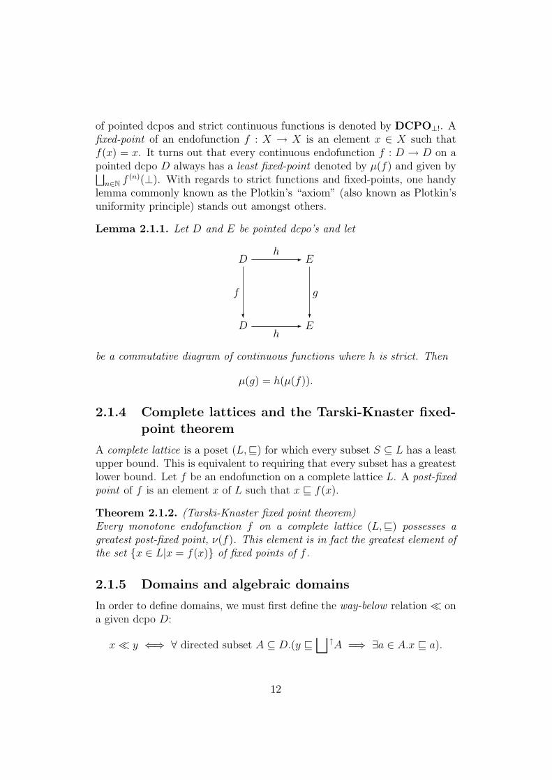
Lemma 2.1.1. Let D and E be pointed dcpo’s and let

Dh

- E

D

f

?

h- E

g

?

be a commutative diagram of continuous functions where h is strict. Then

µ(g) = h(µ(f)).

2.1.4 Complete lattices and the Tarski-Knaster fixed-point theorem

A complete lattice is a poset (L,v) for which every subset S ⊆ L has a leastupper bound. This is equivalent to requiring that every subset has a greatestlower bound. Let f be an endofunction on a complete lattice L. A post-fixedpoint of f is an element x of L such that x v f(x).

Theorem 2.1.2. (Tarski-Knaster fixed point theorem)Every monotone endofunction f on a complete lattice (L,v) possesses agreatest post-fixed point, ν(f). This element is in fact the greatest element ofthe set x ∈ L|x = f(x) of fixed points of f .

2.1.5 Domains and algebraic domains

In order to define domains, we must first define the way-below relation ona given dcpo D:

x y ⇐⇒ ∀ directed subset A ⊆ D.(y v⊔↑A =⇒ ∃a ∈ A.x v a).

12

Using the notion of ideals, the defining condition is equivalent to:

∀X ∈ Id(D).(y v⊔↑X =⇒ x ∈ X).

The following standard properties regarding can be readily verified:

(1) x y =⇒ x v y.

(2) ⊥ x for any x ∈ D.

(3) u v x y v v =⇒ u v.

(4) If u x, v x and u t v exists, then u t v x.

A dcpo D is continuous if for every x ∈ D,

1. the set ↓↓x := d ∈ D|d x is a directed subset of D, and

2.⊔↑ ↓↓x = x.

In the literature, condition (2) is called the axiom of approximation.Moreover, this axiom is equivalent to:

x 6v y =⇒ ∃u x.u 6v y.

The term domain is used throughout this thesis to mean a continuous dcpo.One characteristic feature of a domain is that the relation satisfies thefollowing interpolation property:

x y =⇒ ∃u ∈ D.x u y.

A basis of a domain D is a subset B such that for every x ∈ D, the set ↓↓x∩Bis directed and it holds that

x =⊔↑↓↓x ∩B.

Thus a domain as a subset of itself is a basis. For any basis B of a domainD, the sets ↑↑b for b ∈ B form a base of the Scott topology on D. Thus, ifD and E are domains with bases B and C, then a function f : D → E iscontinuous at x if and only if for every c ∈ C,

c f(x) ⇐⇒ ∃b ∈ B.(b x) ∧ (c f(b)).

13

This is also refered to as the ε-δ characterisation of continuity1. Furthermore

f is continuous ⇐⇒ f(x) =⊔bx

↑f(b).

Given a domain D, an element x ∈ D is finite (or compact) if x x. Inother words, the defining condition is equivalent to:

∀ directed subset A ⊆ D.x v⊔↑A =⇒ ∃a ∈ A.x v a.

Let B be a basis of a domain D. Then by definition of , whenever x y,there exists b ∈ B such that x v b y. This implies that every finiteelement belongs to B. In other words, any basis of a domain contains theset of compact elements. A dcpo D is algebraic if the finite elements form abasis, which we denote by K(D). An example of an algebraic dcpo is Id(D)where D is a dcpo.

The following facts will provide motivation for our definition of opera-tional finiteness in Chapter 10.

Proposition 2.1.3. (e.g. Abramsky and Jung [3], Proposition 2.2.13)If a dcpo D has a countable basis (in the sense of p. 13), then every directedsubset of D contains an ω-chain with the same supremum.

Proposition 2.1.4. Let D be a dcpo with a countable base (in the sense ofp. 13) and ω := ω ∪∞ the ordinal domain. Then the following statementsare equivalent:

(i) x ∈ D is finite.

(ii) For every continuous function f : ω → D, x v f(∞) implies that thereis i ∈ N such that x v f(i).

Proof. (i) ⇒ (ii): Let x ∈ D be finite and f : ω → D a continuous functionwith x v f(∞). Since ∞ =

⊔↑i∈N i and f preserves directed suprema, it

follows that f(∞) =⊔↑

i∈N f(i). Because x is finite, there exists i ∈ N suchthat x v f(i).(ii) ⇒ (i): Assume x ∈ D satisfies the condition of (ii) and suppose furtherthat A ⊆ D is directed with x v

⊔↑A. Then Proposition 2.1.3 ensures theexistence of an ω-chain C in A with

⊔↑C =⊔↑A. The chain C defines

an obvious continuous function c : ω → D and c(∞) =⊔↑A. Thus by

assumption we have i ∈ N such that x v c(i), i.e., there is a ∈ A such thatx v a. So x is finite.

1One can compare this with the formulation of continuity in real analysis.

14

2.2 Essential categorical notions

In this section, we recall some categorical notions used in our operationaltreatment of recursive types.

2.2.1 Limits and colimits

Let C be a category and J a small category. A diagram F in C of type J isa functor F : J → C. For each C-object C, we can define a constant diagram∆J (C) : J → C, j 7→ C. The functor ∆J : C → CJ is called the diagonalfunctor. A natural transformation π from ∆J (C) to some other diagramA consists of morphisms πj : C → A(j) such that for each J -morphismu : j → k, the following triangle commutes:

C

A(j)A(u)

-

f j

A(k)

fk

-

Such a natural transformation is called a cone π : C → A with vertex C.A cone π : L → A with vertex L is universal if for every cone f : C → A,there is a unique mediating morphism g : C → L such that πj g = fj forall j ∈ J . The universal cone π : L → A (or less accurately, its vertex L) iscalled the limit of the diagram A, denoted by

L = lim←J

A.

The dual notion is known as colimit.Many categorical notions can be defined in terms of limits or colimits.

However, we only invoke the use of limits and colimits in the constructionof canonical solutions for recursive domain equations in Section 2.3. Oneimportant aspect of this canonicity is the coincidence of the initial algebrasand the final coalgebras. We define these two categorical notions in the nextsection.

2.2.2 Algebras and coalgebras

Let F be an endofunctor on a category C. An F -algebra is given by an objectA together with a morphism f : F (A) → A, denoted by (A, f). An F -algebra

15

homomorphism from (A, f) to (A′, f ′) is a C-morphism g : A → A′ such thatthe following diagram commutes:

F (A)F (g)

- F (A′)

A

f

?

g- A′

f ′

?

We denote by CF the category of F -algebras and F -algebra homomorphisms.(A, f) is an initial F -algebra if it is an initial object in CT , i.e., for everyF -algebra (A′, f ′), there is a unique algebra homomorphism g : A → A′.The dual notion is known as coalgebra (respectively, final coalgebra). Thefollowing lemma regarding initial algebras is useful.

Lemma 2.2.1. (Lambek’s Lemma)If i : F (A) → A is an initial F -algebra, then i is an isomorphism.

2.2.3 Adjunctions

An adjunction (F, G) between two categories C and D is a pair of functors

F : C → D and G : D → C

such that for all C ∈ C and D ∈ D, there is a bijection between the hom-sets

θ : C(C, GD) ∼= D(FC,D)

natural in C and D.It is well-known that the following are equivalent:

(i) F : C D : G is an adjunction.

(ii) There exists a natural transformation η : idC → GF (called the unit)such that for each C-morphism f : C → GD there is a unique D-

16

morphism h : FC → D such that the left triangle

CηC - GFC FC

GD

Gh

?

f

-

D

h

?

commutes.

(iii) There exists a natural transformation ε : FG → idD (called the counit)such that for each D-morphism g : FC → D there is a unique C-morphism k : C → GD such that the right triangle

GD FGDεD - D

C

k

6

FC

Fk

6

g

-

commutes.

2.2.4 Involutory and locally involutory categories

A locally involutory category2 is a category C with a local involution c : C → Cop,i.e., for all C ∈ C it holds that c(C) = C and for any objects A, B ∈ C thefollowing diagram

C(A, B)c- C(B, A)

C(A, B)

c

?

idC(A

,B) -

commutes in Set.The category of locally involutory categories, LocInvCat, has as ob-

jects the locally involutory categories (C, c) and as morphisms those functors

2The term “locally involutory category” was introduced to me in a personal communi-cation with Paul B. Levy.

17

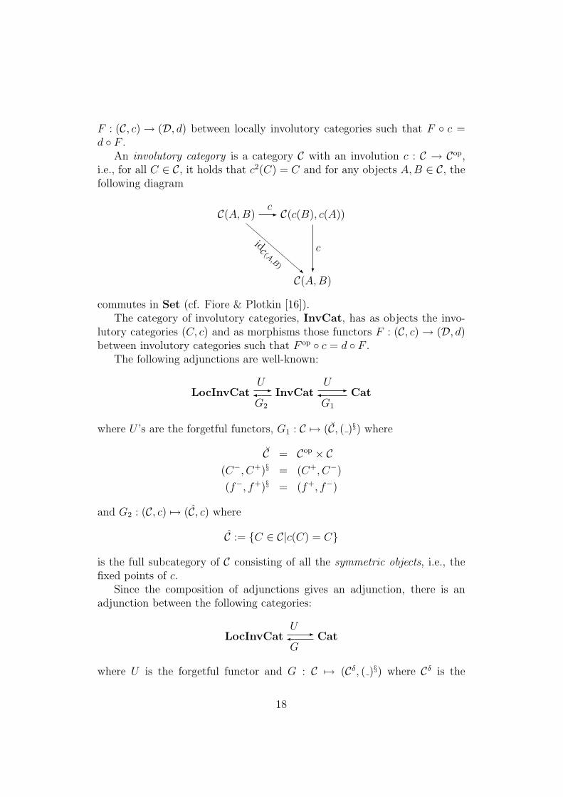
F : (C, c) → (D, d) between locally involutory categories such that F c =d F .

An involutory category is a category C with an involution c : C → Cop,i.e., for all C ∈ C, it holds that c2(C) = C and for any objects A, B ∈ C, thefollowing diagram

C(A, B)c- C(c(B), c(A))

C(A, B)

c

?

idC(A

,B) -

commutes in Set (cf. Fiore & Plotkin [16]).The category of involutory categories, InvCat, has as objects the invo-

lutory categories (C, c) and as morphisms those functors F : (C, c) → (D, d)between involutory categories such that F op c = d F .

The following adjunctions are well-known:

LocInvCatU-

G2

InvCatU

-G1

Cat

where U ’s are the forgetful functors, G1 : C 7→ (C, ( )§) where

C = Cop × C(C−, C+)§ = (C+, C−)

(f−, f+)§ = (f+, f−)

and G2 : (C, c) 7→ (C, c) where

C := C ∈ C|c(C) = C

is the full subcategory of C consisting of all the symmetric objects, i.e., thefixed points of c.

Since the composition of adjunctions gives an adjunction, there is anadjunction between the following categories:

LocInvCatU

-G

Cat

where U is the forgetful functor and G : C 7→ (Cδ, ( )§) where Cδ is the

18

diagonal category, i.e., the full subcategory of C consisting of all the objectson the diagonal.

Note that for every (locally small) category C, we have that (C, ( )§)is an object of InvCat. Morphisms F : (C, ( )§) → (D, ( )§) are functorsF : C → D such that for every f ′ ∈ Cop and for every f ∈ C, it holds thatF1(f

′, f) = F2(f, f ′). Motivated by this example, we call all morphisms inInvCat symmetric functors.

Via the InvCat-Cat adjunction, the involutory categories (B, ( )§) areuniversal in that they are characterised by a natural bijective correspondence

F : C → DF : (C, ( )c)−−−−→symmetric(D, ( )§)

given by the mapping F 7→ F = (F op ( )c, F ).We employ the following technique frequently in Chapter 4 and Chapter

14 to turn mixed variant functors into covariant ones.

Example 2.2.2. Let F : (C)n → C be a functor. Then by the InvCat-Catadjunction, the bijective correspondence gives rise to a symmetric functorF : ((C)n, ( )§) → (C, ( )§) defined by

F (P−1 , P+1 , . . . , P−n , P+

n ) = (F op(P+1 , P−1 , . . . , P−n , P+

n ), F (P−1 , P+1 , . . . , P−n , P+

n ))

F (f−1 , f+1 , . . . , f−n , f+

n ) = (F op(f+1 , f−1 , . . . , f+

n , f−n ), F (f−1 , f+1 , . . . , f−n , f+

n ))

2.3 Recursive domain equations

In this section, we recall some well known results regarding the constructionof canonical solutions of recursive domain equations. We refer the reader toSmyth & Plotkin [56], Streicher [58] and Abramsky & Jung [3] for details ofthese constructions.

We begin by describing the problem in the environment of DCPO⊥ (thecategory of pointed dcpo’s and continuous functions, not necessarily strict).Given an endofunctor F on DCPO⊥, the problem is to find a solution tothe recursive domain equation

F (D) ∼= D

i.e., to construct a pointed dcpo D and an isomorphism fold : F (D) → D.The word “equation” is used to mean “equality up to isomorphisms”. Firstwe must restrict our attention to a particular class of endofunctors. In thiscase, we consider locally continuous endofunctors on DCPO⊥, i.e., those

19

whose morphism part

(D1 → D2) −→ (F (D1) → F (D2))

is a Scott-continuous function for all pointed dcpos D1 and D2. Here (D →E) denotes the function space from D to E, which is defined to be the set ofcontinuous functions f : D → E with respect to the pointwise order. Noticethat functors built from 1 = ⊥ by using functors of the form (−)⊥ (lifting),× (cartesian product) and + (separated sum) are all locally continuous.

2.3.1 Construction of solutions

Let F be a locally continuous endofunctor on DCPO⊥. There are only twomajor steps in solving the recursive domain equation F (D) ∼= D, namely:

(1) Form the dcpo D via a particular limit construction.

(2) Exploit the universal property of limits to obtain the desired isomor-phism fold.

Step 1Denote by 1 = ⊥ the one-point domain and define the sequence of projec-tions (pn : F n+1(1) → F n(1))n∈N by

p0 := λx : F (1).⊥1 and pn := F n(p0).

This gives rise to the following diagram in DCPO⊥

1 p0

F (1) p1

F 2(1) p2

. . . .

whose limit is given by the vertex

Fix(F ) := d ∈∏n∈N

F n(1)|∀n ∈ N.dn = pn(dn+1)

together with the cone of morphisms qn : Fix(F ) → F n(1), d 7→ dn. Theembeddings (en : F n(1) → F n+1(1))n∈N defined by

e0 := λx : 1.⊥F (1) and en := F n(e0)

are such that each (en, pn) is an embedding-projection pair (e-p pair forshort), i.e., pn en = idF (n)(1) and en pn v idF (n+1)(1). Precisely becausethese are e-p pairs, we can further characterise the limit of the sequence(pn)n∈N in a purely local manner as follows:

20

Lemma 2.3.1. Associated to the projections qn’s are the embeddingsin : F n(1) → Fix(F ) defined explicitly by

in(x)m =

(em−1 . . . en)(x) if n ≤ m

(pm . . . pn−1)(x) if n > m

Moreover, we have ⊔n∈N

in qn = idFix(F )

and this property together with the requirement that qn = pn qn+1 charac-terises the limit up to isomorphism.

Step 2Because both (Fix(F ), (qn)n∈N) and (F (Fix(F )), F (qn)n∈N) are limiting conesfor the sequence (pn)n∈N, it follows from the universal properties of theselimiting cones that there is a unique morphism fold : F (Fix(F )) → Fix(F )with qn+1 fold = F (qn) for all n ∈ N. Invoking Lemma 2.3.1, we have:

Lemma 2.3.2. F (Fix(F )) is isomorphic to Fix(F ) via

fold =⊔↑

n∈N in+1 F (qn) : F (fix(F )) → Fix(F )

unfold =⊔↑

n∈N F (in) qn+1 : Fix(F ) → F (Fix(F ))

Moreover, for each n ∈ N, they satisfy the equations:

F (qn) = qn+1 foldF (in) = unfold in+1.

2.3.2 Canonicity

The canonicity of the solution (Fix(F ), fold) of the recursive domain equationF (D) ∼= D can be succinctly captured in the following theorems (due toSmyth & Plotkin [56] but formulated as in Abramsky & Jung [3]) whoseproofs rely crucially on Lemmas 2.1.1, 2.3.1 and 2.3.2.

Theorem 2.3.3. Let F be a locally continuous endofunctor on the categoryof pointed dcpos D and i : F (D) → D be an isomorphism. Then the followingare equivalent:

(i) D ∼= Fix(F ) as F -algebras.

(ii) idD is the least F -algebra endomorphism of D.

21

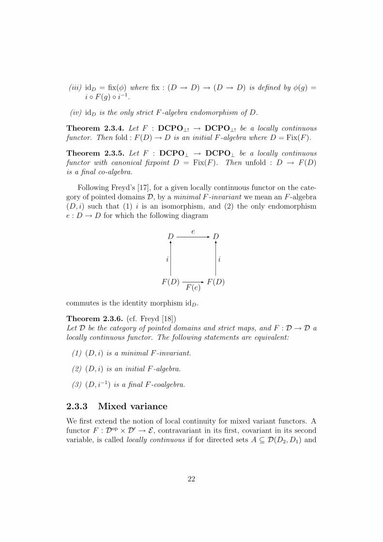
(iii) idD = fix(φ) where fix : (D → D) → (D → D) is defined by φ(g) =i F (g) i−1.

(iv) idD is the only strict F -algebra endomorphism of D.

Theorem 2.3.4. Let F : DCPO⊥! → DCPO⊥! be a locally continuousfunctor. Then fold : F (D) → D is an initial F -algebra where D = Fix(F ).

Theorem 2.3.5. Let F : DCPO⊥ → DCPO⊥ be a locally continuousfunctor with canonical fixpoint D = Fix(F ). Then unfold : D → F (D)is a final co-algebra.

Following Freyd’s [17], for a given locally continuous functor on the cate-gory of pointed domains D, by a minimal F -invariant we mean an F -algebra(D, i) such that (1) i is an isomorphism, and (2) the only endomorphisme : D → D for which the following diagram

De

- D

F (D)

i

6

F (e)- F (D)

i

6

commutes is the identity morphism idD.

Theorem 2.3.6. (cf. Freyd [18])Let D be the category of pointed domains and strict maps, and F : D → D alocally continuous functor. The following statements are equivalent:

(1) (D, i) is a minimal F -invariant.

(2) (D, i) is an initial F -algebra.

(3) (D, i−1) is a final F -coalgebra.

2.3.3 Mixed variance

We first extend the notion of local continuity for mixed variant functors. Afunctor F : Dop × D′ → E , contravariant in its first, covariant in its secondvariable, is called locally continuous if for directed sets A ⊆ D(D2, D1) and

22

A′ ⊆ D′(D′1, D′2) (where D1, D2 are objects in D and D′1, D′2 are objects in

D′) we have

F (⊔↑A,

⊔↑A′) =

⊔f∈A,f ′∈A′

F (f, f ′)

in E(F (D1, D′1), F (D2, D

′2)).

The following theorems (also taken from Abramsky & Jung [3]) will provehandy later.

Theorem 2.3.7. Let D be the category of pointed dcpos and F : Dop×D → Dbe a mixed variant and locally continuous functor. Let i : F (D, D) → D bean isomorphism. Then the following are equivalent:

(i) D ∼= Fix(F ) where Fix(F ) is the limit3 of the diagram:

1 p0

F (1, 1) F (e0, p0)

F (F (1, 1), F (1, 1)) . . .

(ii) idD is the least mixed F -endomorphism of D.

(iii) idD = fix(φ) where φ : (D → D) → (D → D) is defined by φ(g) =i F (g, g) i−1.

(iv) idD is the only strict mixed F -endomorphism of D.

Theorem 2.3.8. Let D⊥! be the category of pointed dcpos and strict maps,and F : Dop

⊥! ×D⊥! → D⊥! be a mixed variant and locally continuous functorand D = Fix(F ). Then for every pair of strict continuous functions f : A →F (B, A) and g : F (A, B) → A there are unique strict functions h : A → Dand k : D → B such that the following diagrams commute:

F (B, A)F (k, h)

- F (D, D) F (D, D)F (h, k)

- F (A, B)

A

f

6

h- D

unfold

6

D

fold

?

k- B

g

?

Given a locally continuous mixed-variant functor F : DCPOop⊥!×DCPO⊥! →

DCPO⊥!, we say that a domain D together with an isomorphism i : F (D, D) →3Interested readers may refer to p. 78 of Abramsky & Jung [3] for the details of the

construction of Fix(F ).

23

D is a bifree solution of X = F (X, X) if every strict e : D → D withe = i F (e, e) i−1 is equal to idD (cf. Streicher [58]).

So with this terminology, (Fix(F ), i) is a bifree solution of X = F (X, X).In view of Theorem 2.3.8, we also say that the canonical solution (Fix(F ), i)a bifree F -algebra.

2.4 Algebraic completeness and compactness

In order to facilitate the discussion of operational algebraic compactness inChapter 14, it is necessary to supply some background information on theconcept of algebraic compactness. The material presented here comes fromfive sources: Freyd [17, 18, 19], Fiore & Plotkin [16] and Fiore [15]. Herewe understand these notions in the setting of DCPO-categories. For anaxiomatic treatment regarding algebraic completeness and compactness, thereader should refer to Fiore & Plotkin [16] and Fiore [15].

By a DCPO-category, we mean a locally small category whose hom-setscome equipped with a directed complete partial order with respect to whichcomposition of morphisms is a continuous operation. Examples of DCPO-categories are DCPO, DCPO⊥! and DCPOop

⊥! ×DCPO⊥!.A DCPO-functor F : C → D between DCPO-categories C and D, con-

sists of a mapping associating every C ∈ C with some F (C) ∈ D and afunctorial mapping associating every C, C ′ ∈ C with some Scott-continuousfunction FC,C′ : C(C, C ′) → D(FC, FC ′). An ordinary functor F : C → Dis said to DCPO-enrich if for every C, C ′ ∈ C, the function FC,C′ is Scott-continuous. As an example, any locally continuous mixed variant functorF : DCPOop

⊥! ×DCPO⊥! is a DCPO-functor.

2.4.1 Parametrised algebraic completeness

A DCPO-category is algebraically complete if every DCPO-functor on ithas an initial algebra.

Let χ and C be DCPO-categories, and F : χ × C → C a DCPO-functor. Assume that C is algebraically complete. For each P ∈ χ, wehave that F (P, ) : C → C is a locally continuous functor so that we canset (F †(P ), iFP ) to be an initial F (P, )-algebra. To extend F † to a functor,we define its morphism part as follows. For every χ-morphism f : P → Q,let F †(f) : F †(P ) → F †(Q) be the unique F (P, )-algebra homomorphism hfrom (F †(P ), iFP ) to (F †(P ), iFQ F (f, F †(Q))), i.e., which makes the following

24

diagram

F (P, F+(P ))iFP - F †(P )

F (P, F †(Q))

F (id, h)

?

F (f, id)- F (Q,F †(Q))

iFQ

- F †(Q)

h

?

commutes. By the universal property of initial algebras, F † is a functorχ → C and, by construction, iF is a natural transformation F (Id, F †) → F †.The pair (F †, iF ) called an initial parametrised F -algebra.

A DCPO-category C is parametrised algebraically complete if it is alge-braically complete and for every DCPO-functor F : χ × C → C and everyfamily iFP : F (P, F †(P )) → F †(P )P∈χ of initial F (P, )-algebras, the in-duced functor F † : χ → C DCPO-enriches.

2.4.2 Parametrised algebraic compactness

A DCPO-category is algebraically compact if it is algebraically complete andthe initial algebra of every DCPO-endofunctor on it is bifree, in the sensethat its inverse is a final coalgebra.

A DCPO-category is parametrised algebraically compact if it is alge-braically compact and parametrised algebraically complete.

Here are some well-known results specialised to the category DCPO⊥! ofpointed dcpos with strict maps.

Proposition 2.4.1. (1) DCPO⊥! is algebraically complete and hence isparametrised algebraically complete.

(2) DCPO⊥! is algebraically compact and hence so is DCPOop⊥!.

2.4.3 The Product Theorem

Theorem 2.4.2. (Product Theorem, Freyd [19], Fiore & Plotkin [16])If C and D are (parametrised) algebraically compact then so is C × D.

Corollary 2.4.3.

(1) If C is (parametrised) algebraically compact then so is Cop.

(2) If C is (parametrised) algebraically compact, so is C.

25

For us, it is important to know, as an example, that DCPOop⊥!×DCPO⊥!

is parametrised algebraically compact.The last property of algebraic compactness (also known as the Funda-

mental Property of Algebraically Compact Categories) is stated below:

Theorem 2.4.4. (Fiore [15]4, Fiore & Plotkin [16])Let χ and C be DCPO-categories. Assume that C is parametrised alge-braically compact. For a symmetric DCPO-functor F : χ × C → C,every initial parametrised F -algebra (F †, iF ) canonically induces an initialparametrised F -algebra (F ‡, ϕF ) such that F ‡ is a symmetric DCPO-functorand ϕ§P = ϕ−1

P for every symmetric P .

4The interested reader is refered to this reference for further explanation concerningthis theorem.

26

Chapter 3

The programming languagePCF

We work with the language1 PCF which is a simply-typed λ-calculus withfunction and finite product types, base types Nat for natural numbers andBool for booleans, as well as fixed-point recursion. For clarity of exposition,we also include a Sierpinski base type Σ and an ordinal base type ω, althoughsuch types can be easily encoded in other existing types if one so desires (forinstance, via retractions - for this, see Scott [50]). We regard this as aprogramming language under the call-by-name2 evaluation strategy.

This chapter introduces the syntax and operational semantics of the lan-guage PCF. In addition, we also bring to the attention of the reader someextensions of PCF which will be useful to us later. Based on Streicher [58](with minor adaptations and simplifications), the material presented here issufficient for us, in Part II, to develop an operational domain and topologyfor the language. However, it is not intended to give a comprehensive intro-duction to the language. For a good reference to PCF, the reader is asked toconsult Streicher [58] and Gunter [24].

3.1 The language PCF

The language PCF is a typed language whose set Type of types is definedinductively as follows:

1PCF (an acronym for Programming language for Computable Functions) was intro-duced by Gordon Plotkin in his paper [42].

2There seems no difficulty developing the results of this thesis in a call-by-value settingas indicated in p. 436 of Escardo & Ho [14] (see also p. 282 of Pitts [41]), and this shoulddefinitely be done.

27

(i) The base types are

(1) Nat: (flat) natural number type,

(2) Bool: Boolean type,

(3) Σ: Sierpinski’s data type, and

(4) ω: ordinal type (or the vertical natural number type).

(ii) Whenever σ and τ are types, then so are σ → τ and σ × τ .

As discussed above, we have included the Sierpinski type Σ and the ordinaltype ω for clarity of exposition. The reader should note that the originalversion of PCF in Plotkin [42] does not include these two data types.

The constructor → is a right associative binary operation on Type mean-ing that, for instance, σ1 → σ2 → σ3 is understood as σ1 → (σ2 → σ2). Theconstructor × is a left associative binary operation on Type, i.e., σ1×σ2×σ3

is taken to mean (σ1 × σ2)× σ3.The first three base types are collectively known as the ground types and

are intended to be types of printable values. We often use the symbol γ torange over ground types.

The PCF raw terms are given by the syntax trees generated by the gram-mar, modulo α-equivalence, in Figure 3.1. Terms of the form s(t) are calledapplications. Terms of the form λx.t are called abstractions. Parenthesesaround applications and abstractions are sometimes omitted with the conven-tion that juxtaposition is left-associative, i.e., t1 . . . tn stands for t1(t2) . . . (tn).

For variables bound by λ’s, we employ the usual convention of α-conversionaccording to which terms are considered as equal if they can be obtained fromeach other by an appropriate renaming of bound variables. Also, when sub-stituting term t for variable x in term s we first rename the bound variables oft in such a way that free variables of s do not get bound by the λ-abstractions,i.e., employing the so-called capture-free substitution.

A type assignment (or typing context) consists of finitely many variablesdeclared together with their types, i.e., it is of the form:

Γ ≡ x1 : σ1, . . . , xn : σn

where the σi’s are the types and the xi’s are pairwise distinct term variables.Formally, a type assignment Γ is a finite partial function from term variablesto types, i.e., dom(Γ) = x1, . . . , xn and Γ : xi 7→ σi (i = 1, . . . , n). Weinductively define terms in valid type assignments of the form Γ ` t : σ(where t is a term of type σ in context Γ) by the typing rules given inFigure 3.2. The letters m, p, s, t range over terms while ∆, Γ range over

28

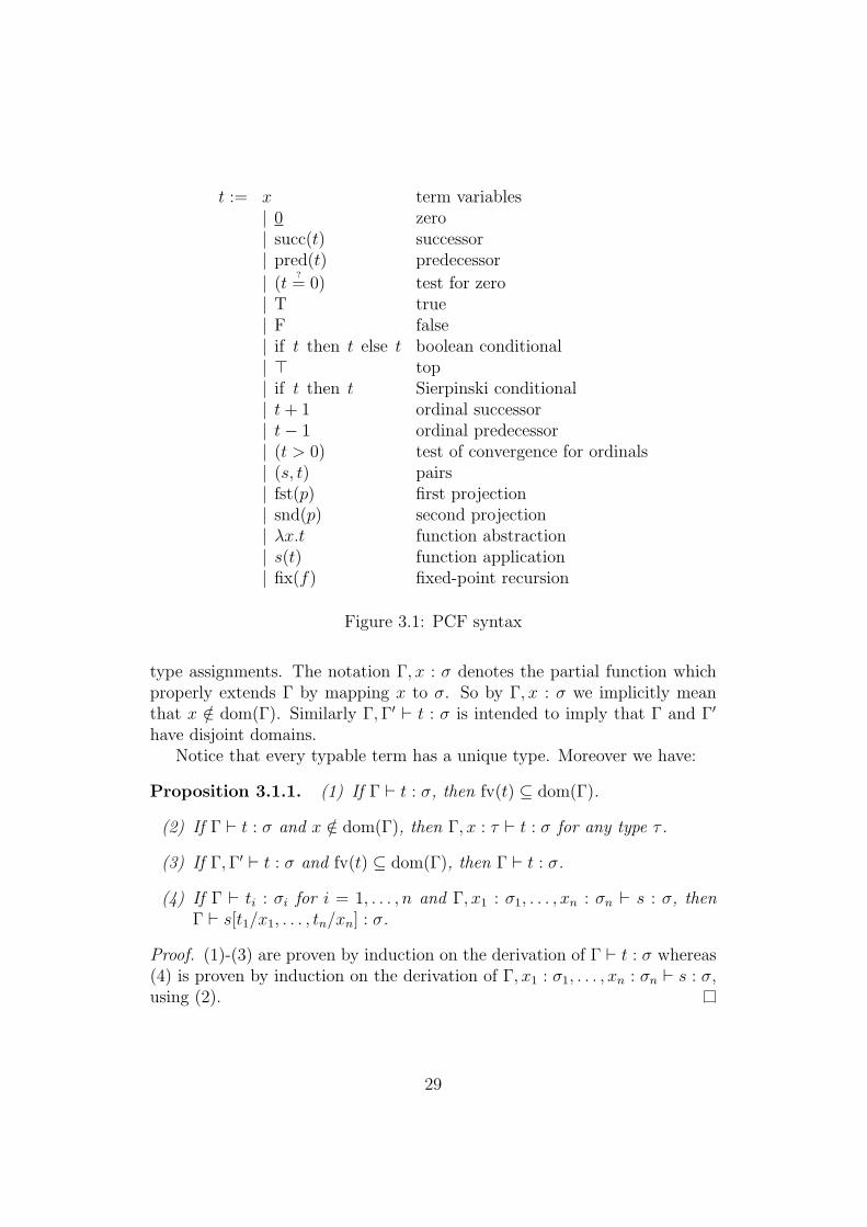
t := x term variables| 0 zero| succ(t) successor| pred(t) predecessor

| (t?= 0) test for zero

| T true| F false| if t then t else t boolean conditional| > top| if t then t Sierpinski conditional| t + 1 ordinal successor| t− 1 ordinal predecessor| (t > 0) test of convergence for ordinals| (s, t) pairs| fst(p) first projection| snd(p) second projection| λx.t function abstraction| s(t) function application| fix(f) fixed-point recursion

Figure 3.1: PCF syntax

type assignments. The notation Γ, x : σ denotes the partial function whichproperly extends Γ by mapping x to σ. So by Γ, x : σ we implicitly meanthat x /∈ dom(Γ). Similarly Γ, Γ′ ` t : σ is intended to imply that Γ and Γ′

have disjoint domains.Notice that every typable term has a unique type. Moreover we have:

Proposition 3.1.1. (1) If Γ ` t : σ, then fv(t) ⊆ dom(Γ).

(2) If Γ ` t : σ and x /∈ dom(Γ), then Γ, x : τ ` t : σ for any type τ .

(3) If Γ, Γ′ ` t : σ and fv(t) ⊆ dom(Γ), then Γ ` t : σ.

(4) If Γ ` ti : σi for i = 1, . . . , n and Γ, x1 : σ1, . . . , xn : σn ` s : σ, thenΓ ` s[t1/x1, . . . , tn/xn] : σ.

Proof. (1)-(3) are proven by induction on the derivation of Γ ` t : σ whereas(4) is proven by induction on the derivation of Γ, x1 : σ1, . . . , xn : σn ` s : σ,using (2).

29

Γ, x : σ ` x : σ(var)

Γ ` 0 : Nat(zero)

Γ ` m : NatΓ ` succ(m) : Nat

(succ)Γ ` m : Nat

Γ ` pred(m) : Nat(pred)

Γ ` T : Bool(true)

Γ ` F : Bool(false)

Γ ` > : Σ(top)

Γ ` s : ωΓ ` (s > 0) : Σ

(> 0)

Γ ` s : ω

Γ ` s + 1 : ω(+1)

Γ ` s : ω

Γ ` s− 1 : ω(−1)

Γ, x : σ ` t : τ

Γ ` (λxσ.t) : σ → τ(abs)

Γ ` s : σ → τ Γ ` t : σΓ ` s(t) : τ

(app)

Γ ` f : σ → σ

Γ ` fixσ(f) : σ(fix)

Γ ` s : σ Γ ` t : τ

Γ ` (s, t) : σ × τ(pair)

Γ ` p : σ × τΓ ` fst(p) : σ

(fst)Γ ` p : σ × τΓ ` snd(p) : τ

(snd)

Γ ` m : Nat

Γ ` m?= 0 : Bool

(?= 0)

Γ ` t : Bool Γ ` s1, s2 : σΓ ` if t then s1 else s2 : σ

(cond)

Γ ` s : Σ Γ ` t : σΓ ` if s then t : σ

(if)

Figure 3.2: Rules for type assignment in PCF

We use the symbol Expσ(Γ) to denote the set of PCF terms that can beassigned the type σ, given Γ:

Expσ(Γ) := t|Γ ` t : σ.

Note that Proposition 3.1.1 implies that all the free variables of t ∈ Expσ(Γ)are contained in dom(Γ). In the special case when t is valid under the emptytyping assignment, we say that it is a closed term, i.e. one with no freevariables. A PCF term with free variables is called an open term. We writeExpσ for Expσ(∅). The elements of Expσ are also called programs of type σ.In particular, programs of ground type are simply known as programs.

3.2 Operational semantics

The big-step operational semantics of PCF is given by the evaluation relationwhich takes the form:

t ⇓ v

30

v ⇓ v(⇓ can)

s ⇓ λxσ.t′ t′[t/x] ⇓ v

s(t) ⇓ v(⇓ app)

f(fix(f)) ⇓ v

fix(f) ⇓ v(⇓ fix)

p ⇓ (s, t) s ⇓ vfst(p) ⇓ v

(⇓ fst)

p ⇓ (s, t) t ⇓ v

snd(p) ⇓ v(⇓ snd)

m ⇓ n

succ(m) ⇓ n + 1(⇓ succ)

m ⇓ 0pred(m) ⇓ 0

(⇓ pred1)m ⇓ n + 1

pred(m) ⇓ n(⇓ pred2)

m ⇓ 0

(m?= 0) ⇓ T

(⇓ (?= 0)1)

m ⇓ n + 1

(m?= 0) ⇓ F

(⇓ (?= 0)2)

t ⇓ T s1 ⇓ vif t then s1 else s2 ⇓ v

(⇓ cond1)t ⇓ F s2 ⇓ v

if t then s1 else s2 ⇓ v(⇓ cond2)

s ⇓ > t ⇓ v

if s then t ⇓ v(⇓ if)

s ⇓ t + 1 t ⇓ vs− 1 ⇓ v

(⇓ (−1))

s ⇓ t + 1(s > 0) ⇓ > (⇓ (> 0))

Figure 3.3: Rules for evaluating PCF terms

where t and v are closed terms and v, the canonical value to which t evaluates,is given by the grammar:

v ::= n | T | F | > | λx.t | (t, t) | t + 1

The set of canonical values is denoted by Valσ. The axioms and rules forinductively defining ⇓ is given in Figure 3.3.

For convenience, we use the following notations.

(1) For each type σ, the symbol ⊥σ (read as bottom) is used to denote theterm fix(λxσ.x).

(2) In ω, define 0 := ⊥ω and for each n ∈ N, the element n : ω is definedto be:

(. . . (0 +1) + 1 . . . ) + 1︸︷︷︸n copies

and the element ∞ : ω is defined as fixω(+1).

The evaluation relation ⇓ is deterministic and preserves typing.

Proposition 3.2.1.

(1) (Determinacy) Whenever t ⇓ v and t ⇓ v′, then v ≡ v′.

31

(2) (Subject reduction) If t ∈ Expσ and t ⇓ v, then v ∈ Expσ.

Proof. Both (1) and (2) can be proven in a straightforward manner by in-duction on the structure of derivation of t ⇓ v.

3.3 Extensions of PCF

In our ensuing development, we shall encounter various extensions of PCFwhich we now describe.

3.3.1 Oracles

PCFΩ is the extension of PCF with the following term-formation rule: Forany function Ω : N → N, computable or not, we have:

Γ ` t : NatΓ ` Ωt : Nat

(oracle).

Then the operational semantics is extended by the rule:

t ⇓ n Ω(n) = mΩt ⇓ m

(⇓ oracle).

We think of Ω as an external input or oracle, and of the equation Ω(n) =m as a query with question n and answer m. Of course, the extension ofthe language with oracle is no longer a programming language. We shallregard it as a data language3. In summary, PCFΩ admits the computationalenvironment in which data supplied may not be programmable in the pro-gramming language. To emphasise that the syntax tree of a closed term isfree of any oracles, we refer to it as a program.

3.3.2 Parallel features

In our study, we also consider PCF extended with certain parallel features.One such extension, PCF+, includes a parallel-or construct (por) with thefollowing term-formation rule:

Γ ` s, t : BoolΓ ` por(s, t) : Bool

(por).

3The term “data language” originates from Escardo [13]

32

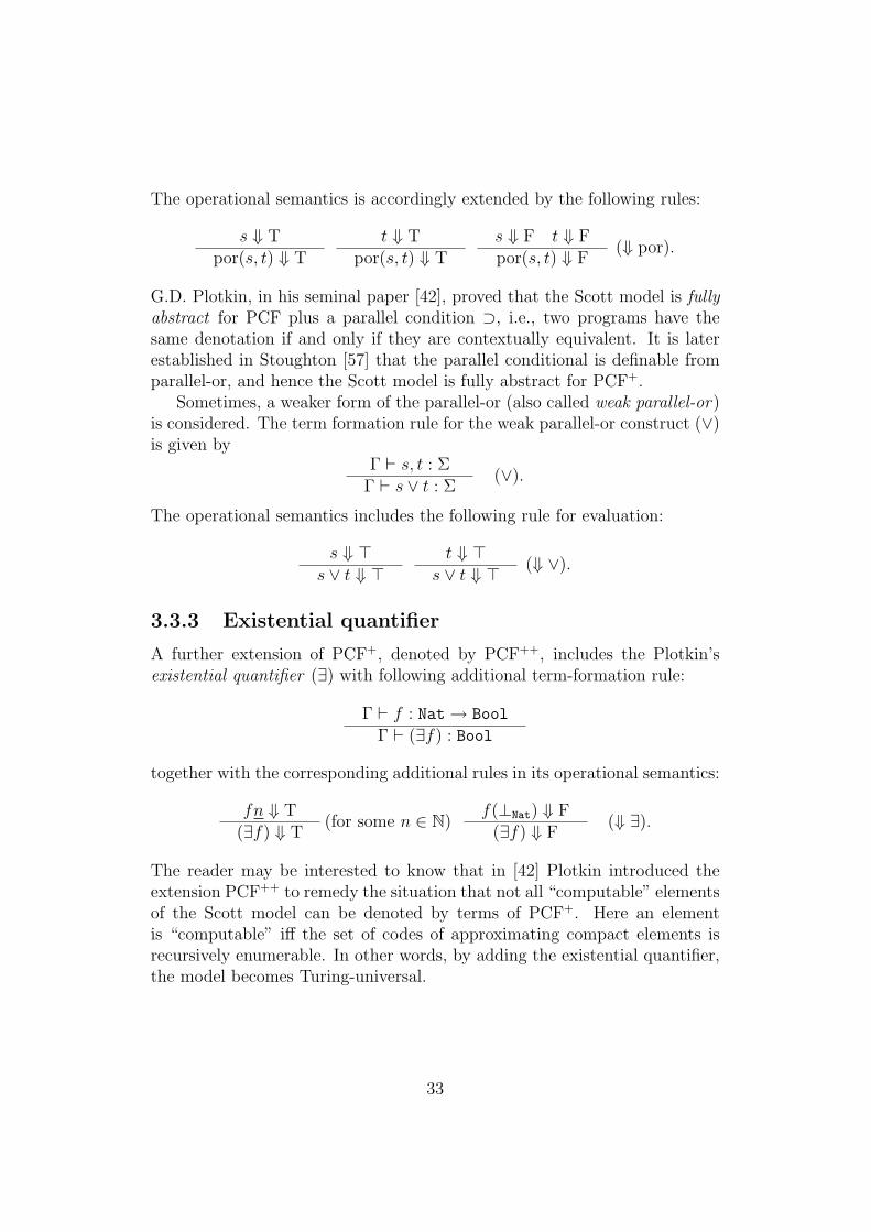
The operational semantics is accordingly extended by the following rules:

s ⇓ Tpor(s, t) ⇓ T

t ⇓ Tpor(s, t) ⇓ T

s ⇓ F t ⇓ Fpor(s, t) ⇓ F

(⇓ por).

G.D. Plotkin, in his seminal paper [42], proved that the Scott model is fullyabstract for PCF plus a parallel condition ⊃, i.e., two programs have thesame denotation if and only if they are contextually equivalent. It is laterestablished in Stoughton [57] that the parallel conditional is definable fromparallel-or, and hence the Scott model is fully abstract for PCF+.

Sometimes, a weaker form of the parallel-or (also called weak parallel-or)is considered. The term formation rule for the weak parallel-or construct (∨)is given by

Γ ` s, t : ΣΓ ` s ∨ t : Σ

(∨).

The operational semantics includes the following rule for evaluation:

s ⇓ >s ∨ t ⇓ >

t ⇓ >s ∨ t ⇓ > (⇓ ∨).

3.3.3 Existential quantifier

A further extension of PCF+, denoted by PCF++, includes the Plotkin’sexistential quantifier (∃) with following additional term-formation rule:

Γ ` f : Nat→ Bool

Γ ` (∃f) : Bool

together with the corresponding additional rules in its operational semantics:

fn ⇓ T(∃f) ⇓ T

(for some n ∈ N)f(⊥Nat) ⇓ F

(∃f) ⇓ F(⇓ ∃).

The reader may be interested to know that in [42] Plotkin introduced theextension PCF++ to remedy the situation that not all “computable” elementsof the Scott model can be denoted by terms of PCF+. Here an elementis “computable” iff the set of codes of approximating compact elements isrecursively enumerable. In other words, by adding the existential quantifier,the model becomes Turing-universal.

33

3.3.4 PCF++Ω

PCF++Ω is the extension of PCF which includes oracles, parallel-or and the

Plotkin’s existential quantifier. It is folkloric4 that the Scott model is abso-lutely universal for PCF++

Ω , i.e., every element of the Scott model becomesdefinable in the language.

3.4 PCF context

One fundamental question in computer science is to determine whether twogiven programs P1 and P2 are the same. It is immediate that one is notconcerned whether they have the same syntax, for what one really cares isthat they exhibit the same behaviour (for instance, whether they completethe same task). The common practice is to put these programs through tests:P1 and P2 are regarded as (observationally) equivalent if and only if they passthe same tests.

In order to formalise the notion of interchanging occurrences of terms inprograms, we use ‘contexts’ - syntax trees containing parameters (or place-holders, or holes) which yield a term when the parameters are replaced byterms.

The PCF contexts, C, are the syntax trees generated by the grammar ofPCF augmented by the clause:

C ::= . . . | p

where p ranges over some fixed set of parameters. Note that the syntax treesof PCF terms are particular contexts, namely the ones with no occurrencesof parameters.

Most of the time we will use contexts involving a single parameter, wewrite as −. We write C[−] to indicate that C is a context containing only oneparameter. If t is a PCF term, then C[t] will denote the term resulting fromchoosing a representative syntax tree for t, substituting it for the parameterin C, and forming the α-equivalence class of the resulting PCF syntax tree(which is independent of the choice of representative for t).

4Only recently did this fact appear in print. For this, see Section 12.15 of [13] andTheorem 13.10 of [59]

34

3.5 Typed contexts

We will assume given a function that assigns types to parameters. We write−σ to indicate that a parameter − has type σ. Just as we only consider aPCF term to be well-formed if it can be assigned a type, we restrict attentionto contexts that can be typed. The relation

Γ ` C : σ

assigning a type σ to a context C given a finite partial function Γ assigningtypes to variables, is inductively generated by axioms and rules just like inFigure 3.2, together with the following axiom for parameters:

Γ ` −σ : σ.

One should take note that when the axioms and rules applied to syntax treesrather than α-equivalence classes of syntax trees (as in the case when typingcontexts), it should be borne in mind that they enforce a separation betweenfree and bound variables and hence are not closed under α-equivalence. Forexample, if x 6= y, then x : Nat ` λy.−Nat : Nat → Nat is a valid typingassertion, whereas x : Nat ` λx.−Nat : Nat→ Nat is not.

Let Ctxσ(Γ) denote the set of PCF contexts that can be assigned type σ,given Γ:

Ctxσ(Γ) := C|Γ ` C : σ.

We write Ctxσ for Ctxσ(∅). Given Γ and C[−σ] ∈ Ctxτ (Γ′), we say that

Γ is trapped within C[−σ] if for each identifier x (i.e., term variable) in Γ,every occurrence of −σ appears in the scope of a binder of x. For example,Γ ≡ x : σ is trapped in the context

C1[−σ] := (λx.−σ)

but not in the context

C2[−σ] := (λx.−σ)(if −σ then 1 else 2).

The operation t 7→ C[t] of substituting a PCF term for a parameter in acontext to obtain a new PCF term respects typing in the following sense:

Lemma 3.5.1. Suppose t ∈ Expσ(Γ, Γ′), C[−σ] ∈ Ctxσ′(Γ) and that Γ′ istrapped within C[−σ]. Then C[t] ∈ Expσ′(Γ).

Proof. By induction on the derivation of Γ ` C[−σ] : σ′.

35

3.6 Contextual equivalence and preorder

Let Γ be a finite partial function from variables to PCF types. Given s, t ∈Expσ(Γ), we write

Γ ` s vσ t

to mean that for all C[−σ] ∈ CtxΣ with Γ trapped within C[−σ],

C[s] ⇓ > =⇒ C[t] ⇓ >.

The relation v is called the contextual preorder between PCF terms (ofthe same type, given a typing of free variables). Contextual equivalence isthe symmetrisation of this relation:

Γ ` s =σ t ⇐⇒ (Γ ` s vσ t) ∧ (Γ ` t vσ s).

For closed terms s, t ∈ Expσ, we just write s vσ t for ∅ ` s vσ t. We alsodefine contextual order to mean the contextual preorder modulo contextualequivalence and denote it by the same symbol v as there will be no confusion.

Remark 3.6.1. The need to apply proofs by induction on the derivationof terms-in-context forces us to define contextual order and equivalence foropen terms, and not just the closed terms.

It does not matter which ground type (i.e., Nat, Bool, Σ) we choose tomake the observation for the testing of programs.

Proposition 3.6.2. The following are equivalent for any terms s, t : σ.

(i) ∀C ∈ CtxΣ.C[s] ⇓ > =⇒ C[t] ⇓ >.

(ii) ∀C ′ ∈ CtxNat.∀n ∈ N.C ′[s] ⇓ n =⇒ C ′[t] ⇓ n.

(iii) ∀C ′′ ∈ CtxBool.∀b ∈ B.C ′′[s] ⇓ b⇒ C ′′[t] ⇓ b.

Proof. We prove only the equivalence of (i) and (ii).(i) ⇒ (ii): Let C ′[−σ] ∈ CtxNat and n ∈ N be given. Suppose that C ′[s] ⇓ n.We want to prove that C ′[t] ⇓ n. To do this, consider the following contextC[−σ] ∈ CtxΣ defined by:

C[−σ] := (C ′[−σ] == n)

36

where x == y is the Sierpinski-valued equality-test on Nat. Note that thisequality test is PCF-definable: (x == y) ≡ fixNat→Nat→Nat(G) where

G ≡ λg.λx.λy.if x?= 0 then (if y

?= 0 then > else ⊥Σ)

else (if y?= 0 then ⊥Σ else g pred(x) pred(y))

Note that for any s ∈ Expσ, C[s] ⇓ > iff C ′[s] ⇓ n. Now invoking (i), wededuce that C[t] ⇓ >. This then implies that C ′[t] ⇓ n as required.(ii) ⇒ (i): Let C[−σ] ∈ CtxΣ be given. Consider the context C ′ ∈ CtxNatdefined by:

C ′ := if C[−σ] then 1.

Note that for any s ∈ Expσ, C ′[s] ⇓ 1 iff C[s] ⇓ >. By applying (ii), wededuce that C ′[t] ⇓ 1 and consequently we have C[t] ⇓ > as required.

3.7 Extensionality and monotonicity

In this section, we record some well-known properties of the contextual pre-order and equivalence which are collectively termed as “extensionality prop-erties” in Pitts [41] (cf. p.255).

Convention and notation. Since our primary focus is the study of thePCF closed terms, we avoid the hassle of writing out all the explicit typingassignments. By an element t of a type σ, we mean the contextual equivalenceclass containing the closed term t of that type. We adopt the set-theoreticnotation for the elements of a type in the sense just defined. For example,write x ∈ σ and f ∈ (σ → τ) to mean that x is an element of type σ and fis an element of type σ → τ . We are going to apply the above convention inSections 3.7 and 6.6, Chapter 5 and in Part III.

Proposition 3.7.1.

(1) For any x, y ∈ γ (where γ is a ground type, i.e., Σ, Nat, Bool),

x vγ y ⇐⇒ ∀v ∈ Valγ.(x ⇓ v ⇒ y ⇓ v).

(2) For any x, y ∈ ω,

x vω y ⇐⇒ ∀s ∈ ω.(x ⇓ s + 1 =⇒ ∃t ∈ ω.y ⇓ t + 1 ∧ s vω t).

37

(3) For any f, g ∈ (σ → τ),

f vσ→τ g ⇐⇒ ∀t ∈ σ.(f(t) vτ g(t)).

(4) For any p, q ∈ (σ × τ),

p vσ×τ q ⇐⇒ (fst(p) vσ fst(q) ∧ snd(p) vτ snd(q)).

The following statements are immediate from the definitions of contex-tual preorder and equivalence, except for the converse of (2) which is a con-sequence of Proposition 3.7.1:

Corollary 3.7.2. (1) Contextual equivalence is a congruence: If f = gand x = y, then f(x) = g(y) for any f, g ∈ (σ → τ) and x, y ∈ σ.

(2) Application is extensional: f = g iff f(x) = g(x) for all x ∈ σ.

(3) Application is monotone: If f v g and x v y, then f(x) v g(y) forany f, g ∈ (σ → τ) and x, y ∈ σ.

38

Chapter 4

The programming languageFPC

We consider a call-by-name version of the language FPC (Fixed Point Cal-culus) whose call-by-value version was first introduced by G.D. Plotkin in his1985 CSLI lecture notes [45]. In a nutshell, FPC does for recursive definitionsof types what PCF does for recursive definitions of functions.

In this chapter, we introduce the syntax and operational semantics of thelanguage FPC. In Part IV, we shall give an operational domain-theoretictreatment of recursive types for this language. The interested reader mayalso find information on call-by-name FPC in McCusker [37] and call-by-value FPC in Gunter [24].

4.1 The language FPC

We assume a set of type variables (ranged over by X,Y , etc.) and the typeexpressions are generated by the following grammar:

σ := X | σ × σ | σ + σ | σ⊥ | µX.σ | σ → σ

For type expressions, we have type variables, product types, sum types, liftedtypes, recursive types and function types. A closed type is a type expressioncontaining no free type variables, i.e., if any occurring type variable X isbound under the scope of a recursive type constructor µX. A type contextis a list of distinct type variables (which may be empty). We write Θ ` σfor the type σ in context Θ, indicating that the set of free type variablesoccurring in σ is a subset of the type context Θ.

The raw FPC terms are given by the syntax trees generated by the fol-lowing grammar, modulo α-equivalence:

39

t := x term variables| (s, t) pairs| fst(p) first projection| snd(p) second projection| inl(t) separated sum| inr(t) separated sum| case(s) of inl(x).t or inr(y).t′ case| up(t) liftings| case(s) of up(x).t case up| fold(t) fold| unfold(t) unfold| λx.t function abstraction| s(t) function application

Figure 4.1: FPC syntax

Terms containing no free variables are called closed terms. Otherwise, theyare known as open terms. A term context is a list of distinct term vari-ables with types. We write Θ; Γ ` t : σ for a term t in (term) contextΓ ≡ x1 : σ1, . . . , xn : σn where Θ ` σi (i = 1, . . . , n) are well-formed types-in-context. When there is no confusion, we omit the type context Θ. Thetyping rules in FPC are given in Figure 4.2.

Convention: We use Θ to range over type contexts; X, Y, R, S over typevariables; ~X, ~Y over sequences of type variables; ρ, σ, τ over type expressions;Γ over term contexts; x, y, z, f, g, h over terms variables; ~f,~g over sequencesof term variables, and s, t, u, v over terms. We write σ[τ/X] to represent theresult of replacing X with τ in the type expression σ (avoiding the captureof bound variables). Similarly, we write s[t/x] to denote capture-free sub-stitution of free occurrences of the variable x in s by the term t. We alsoabbreviate the term context x1 : σ1, . . . , xn : σn as ~x : ~σ.

Lemma 4.1.1. (1) If Γ ` t : σ, then fv(t) ⊆ dom(Γ).

(2) If Γ ` t : σ and x 6∈ dom(Γ), then Γ, x : τ ` t : σ for any τ .

(3) If Γ, Γ′ ` t : σ and fv(t) ⊆ dom(Γ), then Γ ` t : σ.

(4) If Γ ` ti : σi for i = 1, . . . , n and Γ, x1 : σ1, . . . , xn : σn ` s : σ, thenΓ ` s[~t/~x] : σ.

Proof. (1) - (3) are proven by induction on the derivation of Γ ` t : σ and(4) is proven by induction on the derivation of Γ, ~x : ~σ : s : σ, using (2).

40

Γ, x : σ ` x : σ(var)

Γ, x : σ ` t : τ

Γ ` λxσ.t : σ → τ(abs)

Γ ` s : σ → τ Γ ` t : σ

Γ ` s(t) : τ(app)

Γ ` s : σ Γ ` t : τΓ ` (s, t) : σ × τ

(pair)

Γ ` t : σ × τ

Γ ` fst(t) : σ(fst)

Γ ` t : σ × τ

Γ ` snd(t) : τ(snd)

Γ ` t : σ

Γ ` up(t) : σ⊥(up)

Γ ` s : σ⊥ Γ, x : σ ` t : τΓ ` case(s) of up(x).t : τ

(case up)

Γ ` t : σ

Γ ` inl(t) : σ + τ(inl)

Γ ` t : τ

Γ ` inr(t) : σ + τ(inr)

Γ ` s : σ1 + σ2 Γ, x : σ1 ` t1 : τ Γ, y : σ2 ` t2 : τΓ ` case(s) of inl(x).t1 or inr(y).t2 : τ

(case)

Γ ` t : σ[µX.σ/X]Γ ` fold(t) : µX.σ

(fold)

Γ ` t : µX.σΓ ` unfold(t) : σ[µX.σ/X]

(unfold)

Figure 4.2: Rules for type assignments in FPC

Let Expσ(Γ) denote the set of FPC terms that can be assigned the closedtype σ, given Γ, i.e., Expσ(Γ) := t|Γ ` t : σ. We simply write Expσ forExpσ(∅).

4.2 Operational semantics

The operational semantics is given by an evaluation relation ⇓, of the formt ⇓ v, where t and v are closed FPC terms, and v is in canonical form:

v := (s, t) | inl(t) | inr(t) | up(t) | fold(t) | λx.t

A closed term v generated by the above grammar is called a canonical value.Let Valσ denote the set of canonical values of the closed type σ, i.e.,

Valσ := v|∅ ` v : σ.

The relation ⇓ is inductively defined in Figure 4.3 below.

Proposition 4.2.1. Evaluation is deterministic and preserves typing, i.e.,

(1) If t ⇓ v and t ⇓ v′, then v ≡ v′.

41

v ⇓ v(⇓ can)

s ⇓ λx.s′ s′[t/x] ⇓ v

st ⇓ v(⇓ app)

p ⇓ (s, t) s ⇓ v

fst(p) ⇓ v(⇓ fst)

p ⇓ (s, t) t ⇓ vsnd(p) ⇓ v

(⇓ snd)

s ⇓ up(t′) t[t′/x] ⇓ vcase(s) of up(x).t ⇓ v

(⇓ case up)s ⇓ fold(t) t ⇓ v

unfold(t) ⇓ v(⇓ unfold)

s ⇓ inl(t) t1[t/x] ⇓ v

case(s) of inl(x).t1 or inr(y).t2 ⇓ v(⇓ case inl)

s ⇓ inr(t) t2[t/y] ⇓ v

case(s) of inl(x).t1 or inr(y).t2 ⇓ v(⇓ case inr)

Figure 4.3: Rules for evaluating FPC terms

(2) If t ⇓ v and t ∈ Expσ, then v ∈ Expσ.

Proof. Both (1) and (2) are proven by induction on the derivation of t ⇓ v(invoking Lemma 4.1.1(iv)).

4.3 Fixed point operator

Like existing works such as Gunter [24] and Rohr [47], we can define a fixedpoint operator using the recursive types. This is done as follows:

fixσ := λf : (σ → σ).k(foldτ (k))

with τ := µX.(X → σ) and k := λxτ .f(unfoldτ (x)x).We shall prove in Chapter 7 that fix(f) and f(fix(f)) are contextually

equivalent. The reader should note that for this fixed point operator thefollowing evaluation does not hold:

f(fixσ(f)) ⇓ vfixσ(f) ⇓ v

.

4.4 Some notations

In this section, we shall gather at one place the notations which we useregarding the syntax of FPC.

To begin with, there are three special closed types worth mentioning:

1 := µX.X, Σ := 1⊥, ω := µX.(X⊥)

42

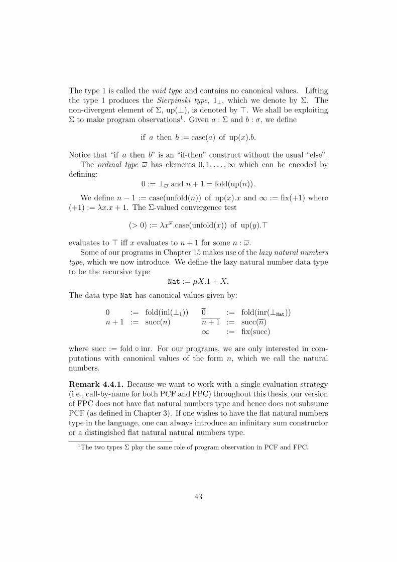
The type 1 is called the void type and contains no canonical values. Liftingthe type 1 produces the Sierpinski type, 1⊥, which we denote by Σ. Thenon-divergent element of Σ, up(⊥), is denoted by >. We shall be exploitingΣ to make program observations1. Given a : Σ and b : σ, we define

if a then b := case(a) of up(x).b.

Notice that “if a then b” is an “if-then” construct without the usual “else”.The ordinal type ω has elements 0, 1, . . . ,∞ which can be encoded by

defining:0 := ⊥ω and n + 1 = fold(up(n)).

We define n − 1 := case(unfold(n)) of up(x).x and ∞ := fix(+1) where(+1) := λx.x + 1. The Σ-valued convergence test

(> 0) := λxω.case(unfold(x)) of up(y).>

evaluates to > iff x evaluates to n + 1 for some n : ω.Some of our programs in Chapter 15 makes use of the lazy natural numbers

type, which we now introduce. We define the lazy natural number data typeto be the recursive type

Nat := µX.1 + X.

The data type Nat has canonical values given by:

0 := fold(inl(⊥1)) 0 := fold(inr(⊥Nat))n + 1 := succ(n) n + 1 := succ(n)

∞ := fix(succ)

where succ := fold inr. For our programs, we are only interested in com-putations with canonical values of the form n, which we call the naturalnumbers.

Remark 4.4.1. Because we want to work with a single evaluation strategy(i.e., call-by-name for both PCF and FPC) throughout this thesis, our versionof FPC does not have flat natural numbers type and hence does not subsumePCF (as defined in Chapter 3). If one wishes to have the flat natural numberstype in the language, one can always introduce an infinitary sum constructoror a distingished flat natural natural numbers type.

1The two types Σ play the same role of program observation in PCF and FPC.

43

C := x term variables| (S, T ) pairs| fst(P ) first projection| snd(P ) second projection| inl(T ) separated sum| inr(T ) separated sum| case(S) of inl(x).T or inr(y).T ′ case| up(T ) liftings| case(S) of up(x).T case up| fold(T ) fold| unfold(T ) unfold| λx.T function abstraction| S(T ) function application| p parameter (or hole)

Figure 4.4: FPC contexts

4.5 FPC contexts

The FPC contexts, C, are syntax trees generated by the grammar for FPCterms in Figure 4.1 augmented by the clause:

C ::= . . . | p

where p ranges over a fixed set of parameters (or holes). The details of thedefining grammar is spelt out in Figure 4.4.

Convention. We use capital letters, for instance, C, T and V to range overFPC contexts.

We assume a function that assigns types to parameters and write −σ

to indicate that a parameter − has closed type σ. We restrict ourselves tocontexts which are typable. The relation

Γ ` C : σ

assigning a closed type σ to a context C given the term Γ, is inductivelygenerated by axioms and rules in Figure 4.5. We define

Ctxσ(Γ) := C|Γ ` C : σ

to be the set of FPC contexts that can be assigned to the closed type σ,

44

Γ, x : σ ` x : σ(var)

Γ, x : σ ` T : τ

Γ ` λxσ.T : σ → τ(abs)

Γ ` S : σ → τ Γ ` T : σ

Γ ` S(T ) : τ(app)

Γ ` S : σ Γ ` T : τΓ ` (S, T ) : σ × τ

(pair)

Γ ` T : σ × τ

Γ ` fst(T ) : σ(fst)

Γ ` T : σ × τ

Γ ` snd(T ) : τ(snd)

Γ ` T : σ

Γ ` up(T ) : σ⊥(up)

Γ ` S : σ⊥ Γ, x : σ ` T : τΓ ` case(S) of up(x).T : τ

(case up)

Γ ` T : σ

Γ ` inl(T ) : σ + τ(inl)

Γ ` T : τ

Γ ` inr(T ) : σ + τ(inr)

Γ ` S : σ1 + σ2 Γ, x : σ1 ` T1 : τ Γ, y : σ2 ` T2 : τΓ ` case(S) of inl(x).T1 or inr(y).T2 : τ

(case)

Γ ` T : σ[µX.σ/X]Γ ` fold(T ) : µX.σ

(fold)

Γ ` T : µX.σΓ ` unfold(T ) : σ[µX.σ/X]

(unfold)

Γ ` −σ : σ(par)

Figure 4.5: Typing rules for FPC contexts

given Γ. We write Ctxσ for Ctxσ(∅).Let Γ ` s, t : σ be two FPC terms-in-context. We write

Γ ` s vσ t

to mean that for all ground contexts C[−σ] ∈ CtxΣ with Γ trapped withinC[−σ],

C[s] ⇓ > =⇒ C[t] ⇓ >.

The relation v is called the contextual preorder and its symmetrisation iscalled the contextual equivalence, denoted by =. For a given term σ, theorder induced by the preorder v on the set of equivalence classes of closedterms of type σ is called the contextual order. Notice that we have chosenthe ground type Σ to be the type on which program observations are based.Such a choice is motivated by aiming for compatibility with PCF (see Section3.6).

Remark 4.5.1. Let s, t : σ be closed terms. Then s vσ t iff

∀p : σ → Σ.(p(s) ⇓ > =⇒ p(t) ⇓ >).

45

Proof. (⇒): For each function p : σ → Σ, define the context C[−σ] ∈ CtxΣ

to be p(−σ).(⇐): Given a context C[−σ] ∈ CtxΣ, define the function p : σ → Σ to beλxσ.C[x] where x is a fresh variable not trapped in C[−σ].

4.6 Denotational semantics

In this section, we give the standard Scott (domain-theoretic) denotationalsemantics for FPC. The reader may consult Fiore & Plotkin [16] and Mc-Cusker [37] for details.

4.6.1 Interpretation of types

Types-in-context Θ ` τ are interpreted as an n-ary symmetric locally con-tinuous functors [[Θ ` τ ]] : (D)n → D where D = DCPO⊥! and this inter-pretation is given in Figure 4.6.

[[Θ ` Xi]] = Πi (1 ≤ i ≤ |Θ|)[[Θ ` τ1 + τ2]] = (Π2[[Θ ` τ1]] + Π2[[Θ ` τ2]])˘

[[Θ ` τ⊥]] = ((Π2[[Θ ` τ ]])⊥)˘

[[Θ ` τ1 × τ2]] = (Π2[[Θ ` τ1]]× Π2[[Θ ` τ2]])˘

[[Θ ` τ1 → τ2]] = (Π1[[Θ ` τ1]] → Π2[[Θ ` τ2]])˘

[[Θ ` µX.τ ]] = [[Θ, X ` τ ]]‡

Figure 4.6: Definition of [[Θ ` Γ]] : (D)|Θ| → D

For the purpose of understanding the above figure, it may be helpful torecall that:

(1) Πi is the projection functor in the ith component.

(2) The notation (−)˘ is as defined in Example 2.2.2.

(3) The notation F ‡ is as defined in Theorem 2.4.4.

The reader may like to consult Section 8.4 of Fiore [15] for a detailed expla-nation of Figure 4.6 above.

The interpretation of types respects a substitution lemma:

46

Lemma 4.6.1. (Substitution lemma for types)There exists a canonical natural isomorphism

β : [[Θ ` σ[τ/X]]] ∼= [[Θ, X ` σ]](Id, [[Θ ` τ ]])

such that β§P = β−1P for all symmetric P .

4.6.2 Interpretation of terms

The interpretation of terms-in-context is standard: variables correspond toprojections, inl/inr correspond to coproduct injections, case correspond tocoproduct selection, (−,−) to pairing, fst/snd to projections, λx.− to cur-rying, −(−) to evaluation and fold/unfold to folding/unfolding a recursivetype. We give the interpretation of terms-in-context of the form Γ ` t : τ inFigure 4.7.

Lemma 4.6.2. (Substitution lemma for terms)Suppose Γ, x : σ ` s : τ and Γ ` t : σ. Then Γ ` s[t/x] : τ and

[[Γ ` s[t/x] : τ ]] = [[Γ, x : σ ` s : τ ]] (id[[Γ]], [[Γ ` t : σ]]).

4.6.3 Soundness and computational adequacy

G.D. Plotkin established in [45] that the Scott model for call-by-value FPCis sound and computationally adequate. With some modifications, it ispossible to establish a similar result for call-by-name FPC.

Theorem 4.6.3. (Soundness and computational adequacy)

(1) The Scott model of call-by-name FPC is correct, i.e., for all s ∈ Expσ

and all v ∈ Valσ, we have

s ⇓ v =⇒ [[s]] = [[v]].

(2) The Scott model of call-by-name FPC is computationally adequate, i.e.,for all s ∈ ExpΣ, we have

[[s]] = > =⇒ s ⇓ >.

Corollary 4.6.4. Let σ be any closed type. Then for all s, t ∈ Expσ, wehave

[[s]] = [[t]] =⇒ s =σ t.

47

For every symmetric P ∈ |D||Θ| we define [[Θ, Γ ` t : τ ]]P as follows:

[[Θ, Γ ` xi]]P = πi (1 ≤ i ≤ |Γ|)[[Θ, Γ ` inl(t) : τ1 + τ2]]P = ι1 [[Γ ` t : τ1]]P

[[Θ, Γ ` inr(t) : τ1 + τ2]]P = ι2 [[Γ ` t : τ2]]P

[[Θ, Γ ` case(s) of

inl(x).t1

inr(y).t2: τ ]]P = [[[Θ, Γ, x : τ1 ` t1 : τ ]]P ,

[[Θ, Γ, y : τ2 ` t2 : τ ]]]P δ 〈id, [[Θ, Γ ` s : τ1 + τ2]]P 〉where δ is the canonical isomorphism

[[Θ, Γ]]× ([[Θ ` τ1]] + [[Θ ` τ2]]) ∼=([[Θ, Γ]]× [[Θ ` τ1]]) + ([[Θ, Γ]]× [[Θ ` τ2]])

[[Θ, Γ ` (s, t) : τ1 × τ2]]P = 〈[[Θ, Γ ` s : τ1]]P , [[Θ, Γ ` t : τ2]]〉P[[Θ, Γ ` fst(t) : τ1]]P = π1 [[Θ, Γ ` t : τ1 × τ2]]P

[[Θ, Γ ` snd(t) : τ2]]P = π2 [[Θ, Γ ` t : τ1 × τ2]]P

[[Θ, Γ ` λx : τ1.t : τ1 → τ2]]P = Λ([[Θ, Γ, x : τ1 ` t : τ2]]P )

[[Θ, Γ ` s(t) : τ2]]P = eval 〈[[Θ, Γ ` s : τ1 → τ2]]P , [[Θ, Γ ` t : τ1]]P 〉

[[Θ, Γ ` fold(t) : µX.τ ]]P = IP [[Θ, Γ ` t : τ [µX.τ/X]]]P

where IP := (ϕ[[X`τ ]]P βP )2

[[Θ, Γ ` unfold(t) : τ [µX.τ/X]]]P = EP [[Θ, Γ ` t : µX.τ ]]P

where EP = I−1P

Figure 4.7: Definition of [[Θ, Γ ` t : τ ]]

48

Chapter 5

Synthetic topology

The material presented in this chapter comes from Escardo [13] in which itis shown, via synthetic topology, how topological concepts can be directly un-derstood in terms of the operational semantics, and, moreover, are applicableto sequential languages. In this section, we introduce operational topologicalnotions that are essential to the development of our theory and these includespace, continuous map, open set, closed set, discrete space, Hausdorff spaceand compact set. Whenever there is no confusion, we shall omit the word‘computational’ as we talk about the various computational topological con-cepts. For instance, we speak of an open set instead of a computationallyopen set.

5.1 Continuous maps

We identify contextually equivalent programs and, by an abuse of notation,we denote by σ the set of closed terms of type σ, modulo contextual equiv-alence. A function from the set σ to the set τ may or may not be definableby a term of type σ → τ . If it is, we say that the function is continuous.Notice that, in a call-by-name framework, such as ours, every term of typeσ → τ is uniquely determined, modulo contextual equivalence, by its func-tional behaviour, by extensionality (cf. Corollary 3.7.2(2)). If f : σ → τ iscontinuous, we use the notation f ∈ (σ → τ).

Since continuity is dependent on the language, varying the language underconsideration will vary the continuity of a given function. In this chapter,we take the internal view of data. So our base language is PCF. But whatwe develop applies just as well to the external view of data, i.e., by changingthe base language to the data language PCFΩ, which we are going to takeup when we come to the notion of compactness.

49

Remark 5.1.1. Continuous maps are programs and are thus monotone withrespect to the contextual order.

Example 5.1.2. There are four functions of type Σ → Σ, namely

(1) f1 : > 7→ ⊥,⊥ 7→ ⊥

(2) f2 : > 7→ >,⊥ 7→ ⊥

(3) f3 : > 7→ >,⊥ 7→ >

(4) f4 : > 7→ ⊥,⊥ 7→ >

It is easy to see that fi (i = 1, 2, 3) are continuous as they can be respectivelydefined by the following programs:

(i) λxΣ.⊥

(ii) λxΣ.x

(iii) λxΣ.>

Notice that f4 cannot be continuous as it fails to be monotone.

5.2 Open and closed subsets

It is well known in classical topology that the notion of open sets can bedefined in terms of continuity. We do the same here.

Definition 5.2.1. A set U of elements of a type σ is open if there is χU ∈(σ → Σ) such that for all x ∈ σ,

χU(x) = > ⇐⇒ x ∈ U.

If such an element χU exists, then it is unique up to contextual equivalence,and we refer to it as the characteristic function of U . A set is called closedif its complement is open.

Example 5.2.2. The subsets ∅, >, ⊥,> of type Σ are open since theircharacteristic functions f1, f2 and f3 are all continuous. But ⊥ is not openas a characteristic function would have violated monotonicity.

As continuity is defined in terms of definability in the language, it istypical that proofs in computational topology are given by programs writtento meet required specifications. One such example is given by the followingproposition which states that programs of functional type are continuous inthe topological sense:

50

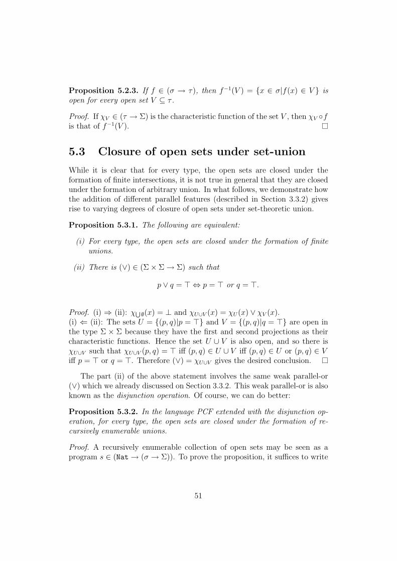
Proposition 5.2.3. If f ∈ (σ → τ), then f−1(V ) = x ∈ σ|f(x) ∈ V isopen for every open set V ⊆ τ .

Proof. If χV ∈ (τ → Σ) is the characteristic function of the set V , then χV fis that of f−1(V ).

5.3 Closure of open sets under set-union

While it is clear that for every type, the open sets are closed under theformation of finite intersections, it is not true in general that they are closedunder the formation of arbitrary union. In what follows, we demonstrate howthe addition of different parallel features (described in Section 3.3.2) givesrise to varying degrees of closure of open sets under set-theoretic union.

Proposition 5.3.1. The following are equivalent:

(i) For every type, the open sets are closed under the formation of finiteunions.

(ii) There is (∨) ∈ (Σ× Σ → Σ) such that

p ∨ q = > ⇔ p = > or q = >.

Proof. (i) ⇒ (ii): χS∅(x) = ⊥ and χU∪V (x) = χU(x) ∨ χV (x).

(i) ⇐ (ii): The sets U = (p, q)|p = > and V = (p, q)|q = > are open inthe type Σ × Σ because they have the first and second projections as theircharacteristic functions. Hence the set U ∪ V is also open, and so there isχU∪V such that χU∪V (p, q) = > iff (p, q) ∈ U ∪ V iff (p, q) ∈ U or (p, q) ∈ Viff p = > or q = >. Therefore (∨) = χU∪V gives the desired conclusion.

The part (ii) of the above statement involves the same weak parallel-or(∨) which we already discussed on Section 3.3.2. This weak parallel-or is alsoknown as the disjunction operation. Of course, we can do better:

Proposition 5.3.2. In the language PCF extended with the disjunction op-eration, for every type, the open sets are closed under the formation of re-cursively enumerable unions.

Proof. A recursively enumerable collection of open sets may be seen as aprogram s ∈ (Nat→ (σ → Σ)). To prove the proposition, it suffices to write

51

a program p ∈ ((Nat → (σ → Σ)) → (σ → Σ)) such that p(s)(x) = > iffs(i)(x) = > for some i ∈ Nat. To meet this requirement, define

p(s) = λx.e(0)

where e is recursively given by e(i) = s(i)(x) ∨ e(i + 1). Then p(s)(x) = >iff e(0) = > iff s(i)(x) = > for some i ∈ Nat.

Remark 5.3.3. For the language PCF extended with only the Plotkin’s ex-istential quantifier ∃, it is also true that the union of a recursively enumerablesequence of opens is open since the weak parallel-or can be defined from ∃.

Notice that even with the inclusion of parallel features, closure underarbitrary unions fails in general. However, the following holds:

Theorem 5.3.4. (Escardo [13], Theorem 4.1)For the language PCF++

Ω , the computational topology coincides with the Scotttopology. In particular, computationally open sets are closed under the for-mation of arbitrary unions.

5.4 Subspace

Frequently we are working with only certain elements of a particular datatype. In view of our topological development, it is natural to speak of asubspace as an arbitrary subset of a data type. For instance, σ, in itself, is atrivial subspace. If X is a subspace of σ, then we call σ an environment forspace X.

The subspace N of Nat of non-divergent (i.e. non-bottom) elements isthe space of natural numbers. The data type Nat → Nat is called the Bairedata type and is denoted by Baire. The Baire space is the subset B ofstrict total functions of type Baire. The Cantor space is the subset C of Bconsisting of functions taking values 0 or 1 on all non-divergent arguments.So B (respectively, C) is an operational manifestation of the Baire space(respectively, Cantor space) in classical topology.

Since subspaces of data types are not necessarily data types, we are forcedto work with relative topology. Let X and Y be subspaces of data types σand τ . We say that a function φ : X → Y is relatively continuous if there isat least one continuous function f : σ → τ with φ(x) = f(x) for every x ∈ X.It does not concern us how f behaves outside on elements of σ outside X.We say that a subset of a space is relatively open if its Sierpinski-valuedcharacteristic map is relatively continuous. The following is immediate fromthe definitions.

52

Proposition 5.4.1. For a subspace X of a data type σ, a subset U of X isopen in X iff there is an open subset U ′ of σ such that X ∩ U ′ = U .

Proof. (⇒) Suppose U ⊆ X is relatively open in X. Then there is a con-tinuous function f : σ → Σ such that χU(x) = f(x) for all x : σ. Nowdefine U ′ = f−1(>), which is certainly an open subset of σ and by def-inition χU ′ = f . It is clear that for each x ∈ U , f(x) = > which im-plies that χU ′(x) = >, i.e. x ∈ U ′. Conversely if x ∈ X ∩ U ′, thenχU(x) = f(x) = χU ′(x) = >, i.e. x ∈ U . This proves that X ∩ U ′ = U .(⇐) Suppose that X ∩U ′ = U for some open subset U ′ of σ. The character-istic function χU ′ of U ′ is continuous and thus that of U is since χU = χU ′

when restricted to the subspace X.

Example 5.4.2. (Exercise 3.6 of Escardo [13])The subset of all sequences s which belong to the Baire space and satisfys(17) = 0 is open in B but not open in Baire. For the first part, we mustprove that T is open in B. To do so, observe that T = C ∩U where χU(s) :=if s(17) == 0 then >. The desired result then follows from Proposition5.4.1. We prove the second part when we revisit this example in Chapter 10.

5.5 Separation axioms

In classical topology, it is traditional to study the various degrees of sepa-ration. Roughly speaking, we want to use the open neighbourhoods of thetopology to distinguish between two points in space. Various degrees of sep-aration arise when one considers different manners in which the distinctionbetween points is to be made in terms of their open neighbourhoods. Forinstance, a space is T0 if we require that there is at least one neighbour-hood which contains exactly one of the two distinct points. A space is T1

if we want to have two opens, each containing exactly one of the points. Aspace which satisfy yet a finer separation axiom that requires further thatthe abovementioned pair of opens be non-overlapping is called a Hausdorffspace. An extreme case of Hausdorff separation arises when every singletonis open, i.e., equivalently, the space is discrete, in which every subset is open.

In our setting, the “equality” of programs really means contextual equiv-alence. So different separation conditions translate into the varying degreesof ability to tell two contextually inequivalent programs apart.

A subspace X of type σ is Hausdorff if there exists an apartness program(6=) ∈ (σ × σ → Σ) such that for every x, y ∈ X,

(6=)(x, y) = > ⇐⇒ x 6= y.

53

Here, 6= means contextually inequivalent.A subspace X of type σ is discrete if there exists an equality test (=) ∈

(σ × σ → Σ) such that for every x, y ∈ X,

(=)(x, y) = > ⇐⇒ x = y.

Here, = refers to contextual equivalence.

Example 5.5.1. Any non-trivial data type is not Hausdorff since every openthat contains the bottom element ⊥ must contain every element of that type.

Example 5.5.2. The space of natural numbers, N , is Hausdorff since theapartness map (6=) is realised by the following recursion:

(6=)(x, y) = if x?= 0 then a else b

where the subprograms a and b are defined as follows:

a = if y?= 0 then ⊥ else >

b = if y?= 0 then > else (6=)(pred(x), pred(y))

Notice that also N is (relatively) discrete since we have a recursive recipe forthe closed term which tests for equality on the natural numbers:

(=)(x, y) = if x?= 0 then a else b

where the subprograms a and b are given by:

a = if y?= 0 then > else ⊥

b = if y?= 0 then ⊥ else (=)(pred(x), pred(y))

The natural numbers type Nat, however, is not discrete since we always needto consider the divergent element ⊥.

Example 5.5.3. The Baire space is not discrete since operationally we needto test for equality on each term of the sequence. We omit the proof of thissince this is similar to Example 5.4.2 . One may be tempted to claim thatit is not possible to have an equality (or even apartness) test whenever wedeal with data types that seemingly require one to check an infinitude ofdata for equality. However, this is not true as already shown by Gandy andBerger (cf. Berger [6]). We shall recall these examples and study them in anoperational setting.

54

Example 5.5.4. Given a pair of elements (s, t) ∈ Baire × Baire, considerthe program apart ∈ Nat→ Σ which is recursively defined as follows:

apart(i) = if s(i) 6= t(i) then > else apart(i + 1)

where (6=) is the inequality test on Nat. This program evaluates to > iff thesequences s and t disagree somewhere from the ith position onwards. So theprogram

apartB(s, t) = apart(0)

is the required inequality test, thus justifying that the Baire space is Haus-dorff.

The following proposition1 might be worth noting that

Proposition 5.5.5. In a discrete space, singletons consisting of definableelements are open.

Proof. Let x ∈ σ be a member of a discrete space X. Then the characteristicfunction of the singleton x is given by χx(y) = (=)(x, y) where (=) is theexisting equality test available from the discreteness of X.

Remark 5.5.6. At the time of writing, it is not clear whether an exampleof a discrete non-Hausdorff subspace exists.

5.6 Specialisation order

Recall that the specialisation order v of a T0 space X is defined by

x v y def⇔ ∀ open set U.(x ∈ U =⇒ y ∈ U).

The following says that the contextual order is the “specialisation order” ofthe operational topology:

Proposition 5.6.1. For x, y ∈ σ, the relation x v y holds iff x ∈ U impliesy ∈ U for every open subset U of σ.

Proof. Ground contexts of type Σ suffices to test the operational preorder -see Proposition 3.6.2. Because x and y are closed terms, applicative contexts,i.e., characteristic functions of open sets, suffice.

Remark 5.6.2. For any x 6= y ∈ σ (i.e., contextually inequivalent), thereis an open that contains exactly one of them. This means our operationaltopology is always “T0”.

1In the process of making minor modifications in this thesis, this proposition has beenstrengthened: In a discrete space, singletons are always open.

55

5.7 Compact sets

The intuition behind the topological notion of compactness is that a com-pact set behaves, in many important aspects, as if it were a finite set. Theofficial topological definition, which is more obscure, says that a subset Q isa topological space is compact iff it satisfies the Heine-Borel property: anycollection of open sets that cover Q has a finite subcollection that alreadycovers Q. In order to arrive at an operational notion of compactness, wereformulate this in two stages.

(1) Any collection of open sets of a topological space can be made directedby adding the unions of finite subcollections. Hence a set Q is compactiff every directed cover of Q by open sets includes an open set thatalready covers Q.

(2) Considering the Scott topology on the lattice of open sets of the topo-logical space, this amounts to saying that the collection of open sets Uwith Q ⊆ U is Scott open in this lattice.

Thus this last reformulation considers open sets of open sets. We take this asour definition, with “Scott open” replaced by “open” in the sense of Definition5.2.1: we say that a collection U of open sets of type σ is open if the collectionχU | U ∈ U is open in the function type (σ → Σ).

Proposition 5.7.1. For any set Q of elements of a type σ, the following twoconditions are equivalent:

(i) The collection U is open | Q ⊆ U is open.

(ii) There is ∀Q ∈ ((σ → Σ) → Σ) such that

∀Q(p) = > ⇔ ∀x ∈ Q.p(x) = >.

Proof. ∀Q = χU for U = χU | Q ⊆ U, because if p = χU then Q ⊆ U ⇐⇒p(x) = > for all x ∈ Q.

Definition 5.7.2. We say that a set Q of elements of a type σ is compactif it satisfies the above equivalent conditions. In this case, for the sake ofclarity, we write “∀x ∈ Q. . . . ” instead of “∀Q(λx. . . . )”.

Proposition 5.7.1(2) gives a sense in which a compact set behaves likea set of finite cardinality: it is possible to universally quantify over it in amechanical fashion. So it is not surprising that

56

Proposition 5.7.3. Every finite set of any type is compact.

Proof. Let Q = q1, . . . , qn be finite set. Then the program ∀Q(p) = p(q1)∧p(q2)∧ · · · ∧ p(qn) (where x∧ y := if x then y as previously defined) satisfiesthe condition that ∀Q(p) = > iff ∀x ∈ Q.p(x) = >.

We postpone the examples of infinite compact sets till we revisit com-pactness in Chapter 11.

5.8 Properties of compact sets

Properties of compact sets that are familiar from classical topology hold forour operational notion:

Proposition 5.8.1. (1) The empty set is compact. If Q1 and Q2 are com-pact subsets of the same type then Q1 ∪Q2 is again compact.

(2) For any f ∈ (σ → τ) and any compact set Q in σ, the set f(Q) =f(x) | x ∈ Q is compact in τ .

(3) If Q is compact in σ and R is compact in τ , then Q×R is compact inσ × τ .

(4) If Q is compact in σ and V is open in τ , then

N(Q, V ) := f ∈ (σ → τ) | f(Q) ⊆ V

is open in (σ → τ).

Proof. (1): ∀z ∈ Q1 ∪Q2.p(z) = ∀z ∈ Q1.p(z) ∧ ∀z ∈ Q2.p(z).

(2): ∀y ∈ f(Q).p(y) = ∀x ∈ Q.p(f(x)).

(3): ∀z ∈ Q×R.p(z) = ∀x ∈ Q.∀y ∈ R.p(x, y).

(4): χN(Q,V )(f) = ∀x ∈ Q.χV (f(x)).

Remark 5.8.2. For (3) of the above proposition, open sets of this form areknown in classical topology: They form the subbase that defines the so-calledcompact-open topology on the set of continuous maps.

Example 5.8.3. The set of all elements of any type σ is compact, butfor trivial reasons: p(x) = > holds for all x ∈ σ iff it holds for x = ⊥,by monotonicity, and hence the definition ∀σ(p) = p(⊥) gives a universalquantification program.

57

The following properties of compact sets are also familiar to us fromclassical topology:

Proposition 5.8.4. If X is Hausdorff and Q ⊆ X is compact, then Q isclosed in X.

Proof. It boils down to showing that X\Q is open, i.e., its characteristic mapχX\Q ∈ (σ → Σ). But it is easy to see that the following program does therequired job: χX\Q(x) = ∀y ∈ Q.(6=)(x, y).

Proposition 5.8.5. In the presence of the disjunction operator (∨), if X iscompact and F ⊆ X is closed then F is compact.

Proof. The required program is ∀x ∈ X.χX\F (x) ∨ p(x).

A collection Q of opens of a type σ is said to be compact if the corre-sponding set of characteristic maps

U is open | U ∈ Q

is compact in (σ → Σ).

Proposition 5.8.6. If a set Q of opens is compact, then its intersection⋂Q

is open.

Proof. The required program ∀U ∈ Q.χU(x) satisfies the property that ∀U ∈Q.χU(x) = > iff x ∈ U for all U ∈ Q iff x ∈

⋂Q.

58

Part II

Operational Toolkit

59

In Pitts [41], A. Pitts developed some mathematical methods for rea-soning about program properties based upon the operational semantics of alanguage PCFL, in contrast to methods based upon domain-theoretic deno-tational semantics. In his paper, Pitts showed how the notion of bisimula-tion, together with a certain co-induction principle, can be used to establishprogram equivalence.

We show how Pitts’ methods can be adapted to work for both PCF andFPC. For readers who want to understand operational domain theory andtopology of PCF in Part III but do not wish to spend time on recursive typesmay refer to Chapter 6 and skip Chapters 7 and 8.

In Chapter 6, we only show the necessary modifications for PCF and omitthe proofs. In Chapter 7, the reworking in FPC is shown in full detail. InChapter 8, the proof of the operational extensionality theorem is provided.The reader should note reworking Pitts’ work [41] for the languages PCF andFPC requires hard work but little insight.

60

Chapter 6

Contextual equivalence andPCF bisimilarity

In this chapter, we develop operational machinery to reason about contextualequivalence of PCF programs. We do this by using bisimulation techniquesand the co-induction principle. As an example of how these principles maybe applied, we study the contextual preorder of the ordinal data type ω inSection 6.5.

6.1 Bisimulation and bisimilarity

Throughout this section, we will be concerned with one particular completelattice, (Rel,≤). The elements of Rel are typed-indexed families

R= Rσ |σ ∈ Type

of binary relations Rσ between closed PCF terms of type σ. Thus eachcomponent of R is a subset Rσ⊆ Expσ × Expσ. The partial ordering on Relis defined to be set-theoretic inclusion in each component:

R ≤ R′ def⇔ ∀σ ∈ Type.Rσ ⊆ R′σ.

Clearly the least upper bound of a subset of Rel is given by set-theoreticunion in each component.

Given R∈ Rel, 〈R〉 and [R] are defined in Figure 6.1.Clearly, R7→ 〈R〉 and R7→ [R] are both monotone operators on Rel. So

we can apply Theorem 2.1.2 and form their greatest (post-)fixed points.A family of relations S ∈ Rel satisfying S ≤ 〈S〉 is called a PCF simu-

lation; the greatest such is called PCF similarity and written . A family

61

(1) 〈R〉:

t〈R〉Σt′ ⇐⇒ (t ⇓ > ⇒ t′ ⇓ >) (6.1)

s〈R〉Nats′ ⇐⇒ ∀n ∈ N.(s ⇓ n ⇒ s′ ⇓ n) (6.2)

b〈R〉Boolb′ ⇐⇒ ∀b ∈ B.(b ⇓ b⇒ b′ ⇓ b) (6.3)

s〈R〉ωs′ ⇐⇒ ∀t : ω.(s ⇓ t + 1 ⇒ (6.4)

∃t′ : ω.(s′ ⇓ t′ + 1 ∧ t Rω t′))

f〈R〉σ→τf′ ⇐⇒ ∀t ∈ Expσ.(f(t) Rτ f ′(t)) (6.5)

p〈R〉σ×τp′ ⇐⇒ (fst(p) Rσ fst(p′) ∧ snd(p) Rτ snd(p′)) (6.6)

(2) [R]:

t[R]Σt′ ⇐⇒ (t ⇓ > ⇔ t′ ⇓ >) (6.7)

s[R]Nats′ ⇐⇒ ∀n ∈ N.(s ⇓ n ⇔ s′ ⇓ n) (6.8)

b〈R〉Boolb′ ⇐⇒ ∀b ∈ B.(b ⇓ b ⇐⇒ b′ ⇓ b) (6.9)

s[R]ωs′ ⇐⇒ ∀t : ω.(s ⇓ t + 1 =⇒ (6.10)

∃t′ : ω.(s′ ⇓ t′ + 1 ∧ t Rω t′))

and

∀t′ : ω.(s′ ⇓ t′ + 1 =⇒∃t : ω.(s ⇓ t + 1 ∧ t Rω t′))

f [R]σ→τf′ ⇐⇒ ∀t ∈ Expσ.(f(t) Rτ f ′(t)) (6.11)

p[R]σ×τp′ ⇐⇒ (fst(p) Rσ fst(p′) ∧ snd(p) Rτ snd(p′)) (6.12)

Figure 6.1: Definitions of 〈R〉 and [R] in PCF

of relations B ∈ Rel satisfying B ≤ [B] is called a PCF bisimulation; thegreatest such is called PCF bisimilarity and written as '.

In other words, a simulation is a post-fixed point of the operator 〈〉 and asimilarity is the greatest (post-)fixed point of the operator 〈〉. Similarly, fora bisimulation and a bisimilarity.

We shall pause for a while to spell out what the conditions S ≤ 〈S〉 andB ≤ [B] mean. A simulation S is specified by a type-indexed family of binaryrelations, Sσ ⊆ Expσ × Expσ, satisfying the conditions in Figure 6.2.

Similarly, a bisimulation is specified by a type-indexed family of binaryrelations, Bσ ⊆ Expσ × Expσ, satisfying the conditions in Figure 6.3.

Remark 6.1.1. Note that by Theorem 2.1.2, similarity and bisimilarity are

62

(t SΣ t′ ∧ t ⇓ >) =⇒ t′ ⇓ > (sim 1)(s SNat s′ ∧ s ⇓ n) =⇒ s′ ⇓ n (sim 2)(b SBool b′ ∧ b ⇓ b) =⇒ b′ ⇓ b (sim 3)(s Sω s′ ∧ s ⇓ t + 1) =⇒ ∃t′.(s′ ⇓ t′ + 1 ∧ t Sω t′) (sim 4)f Sσ→τ F ′ =⇒ ∀t ∈ Expσ.(f(t) Sτ f ′(t)) (sim 5)p Sσ×τ p′ =⇒ (fst(p) Sσ fst(p′) ∧ snd(p) Sτ snd(p′)) (sim 6)

Figure 6.2: PCF simulation conditions

(t BΣ t′ ∧ t ⇓ >) =⇒ t′ ⇓ > (bis 1a)(t BΣ t′ ∧ t′ ⇓ >) =⇒ t ⇓ > (bis 1b)(s BNat s′ ∧ s ⇓ n) =⇒ s′ ⇓ n (bis 2a)(s BNat s′ ∧ s′ ⇓ n) =⇒ s ⇓ n (bis 2b)(b BBool b′ ∧ b ⇓ b) =⇒ b′ ⇓ b (bis 3a)(b BBool b′ ∧ b′ ⇓ b) =⇒ b ⇓ b (bis 3b)(s Bω s′ ∧ s ⇓ t + 1) =⇒ ∃t′.(s′ ⇓ t′ + 1 ∧ t Bω t′) (bis 4a)(s Bω s′ ∧ s′ ⇓ t′ + 1) =⇒ ∃t.(s ⇓ t + 1 ∧ t Bω t′) (bis 4b)f Bσ→τ f ′ =⇒ ∀t ∈ Expσ.(f(t) Bτ f ′(t)) (bis 5)p Bσ×τ p′ =⇒ (fst(p) Bσ fst(p′) ∧ snd(p)Bσsnd(p′)) (sim 6)

Figure 6.3: PCF bisimulation conditions

fixed points (rather than just post-fixed points) of their associated monotoneoperators.

6.2 Co-induction principle

In this section, we present a powerful and important proof technique calledthe co-induction principle.

Proposition 6.2.1. (Co-induction principle for and ': PCF)Given s, t ∈ Expσ, to prove that s 'σ t holds, it suffices to find a bisimulationB such that s Bσ t. Similarly, to prove s σ t, it suffices to find a simulationS with s Sσ t.

Proposition 6.2.2. PCF similarity is a preorder and PCF bisimilarity isthe equivalence relation induced by it. In other words, for all types σ and allclosed terms t, t′, t′′ ∈ Expσ, one has:

(1) t σ t.

(2) (t σ t′ ∧ t′ σ t′′) ⇒ t σ t′′.

(3) t 'σ t′ ⇔ (t σ t′ ∧ t′ σ t).

63

6.3 Operational extensionality theorem

We extend and ' from closed terms to all typable PCF terms by consid-ering closed instantiations of open terms. For convenience, we introduce anotation for this process.

Suppose R∈ Rel. For any finite partial function Γ assigning types tovariables

Γ ≡ x1 : σ1, . . . , xn : σn

for any type σ, and for any terms s, s′ ∈ Expσ(Γ), define

Γ ` s Rσ s′ iff ∀t1 ∈ Expσ1, . . . , tn ∈ Expσn

.(s[~t/~x] Rσ s′[~t/~x]).

We call R the open extension of R. Applying this construction to and', we get relations and ' on open terms, which we call open similarityand open bisimilarity respectively.

With these definitions, we can state the following characterisation of con-textual equivalence.

Theorem 6.3.1. (Operational extensionality theorem for PCF)Contextual preorder (respectively, equivalence) coincides with open similarity(respectively, open bisimilarity):

Γ ` s vσ t ⇐⇒ Γ ` s σ t

andΓ ` s =σ t ⇐⇒ Γ ` s 'σ t.

In particular, the following co-induction principle for contextual equivalenceholds: To prove that two closed terms are contextually equivalent, it sufficesto find a bisimulation which relates them.

The techniques involved in proving the above theorem are similar to thosefor establishing Theorem 7.4.4 (Operational extensionality theorem for FPC)whose proof is presented in Chapter 8.

6.4 Kleene preorder and equivalence

For each type σ, consider the following binary relations on Expσ:

s vklσ t def⇔ ∀v ∈ Valσ.(s ⇓ v ⇒ t ⇓ v)

ands ∼=kl

σ t def⇔ (s vklσ t) ∧ (t vkl

σ s).

64

The relation vkl is called the Kleene preorder. If s ∼=klσ t holds we say that s

and t are Kleene equivalent.

Proposition 6.4.1. For each type σ, we have

s vklσ t =⇒ s σ t

ands ∼=kl

σ t =⇒ s 'σ t.

Hence in view of Theorem 6.3.1, Kleene equivalent closed terms are contex-tually equivalent.

The following contextual equivalences of open terms follow immediatelyfrom the fact that they are all Kleene equivalences:

(λx.s)t = s[t/x]

fst(s, t) = s

snd(s, t) = t

if T then s else s′ = s

if F then s else s′ = s′

if > then t = t

(n + 1)− 1 = n

0− 1 = 0

∞+ 1 = ∞fix(f) = f(fix(f))

Proposition 6.4.2. For each type σ, ⊥σ := fix(λxσ.x) is the least elementof type σ with respect to the contextual order.

Proof. Notice that since ⊥σ does not evaluate to anything, we have that

⊥σ vklσ t

for any t ∈ Expσ. By Proposition 6.4.1, we deduce that ⊥σ acts as the leastelement with respect to the contextual preorder.

Remark 6.4.3. In ω, the elements (0− 1) + 1 and 1 are distinct canonicalvalues which are contextually equivalent. This just indicates that the Kleeneequivalence is strictly contained in the contextual equivalence. Also it followsfrom Kleene equivalence and transitivity of contextual equivalence that if∅ ` s =σ t and s ⇓ u and t ⇓ v, then ∅ ` u =σ v.

65

6.5 Elements of ordinal type

In this section, we show that the contextual order of the ordinal type ω isindeed the ordinal domain:

0 <ω 1 <ω · · · <ω n <ω · · · <ω ∞.

In other words, we shall prove that the closed terms 0, 1, . . . ,∞ are contex-tually inequivalent terms of type ω. Diagrammatically, the contextual orderof ω is given in Figure 6.4.

bbb...

b

0 = ⊥1

2

∞

Figure 6.4: Vertical natural numbers: ω

At this juncture, the reader may refer to Section 3.2 to recall the definitionof 0, . . . , n, . . . ,∞.

To understand the contextual order of ω, we first consider a relation Sbetween closed terms defined as follows:

t SΣ t′ ⇐⇒ (t ⇓ > =⇒ t′ ⇓ >).

s SNat s′ ⇐⇒ (∀n ∈ N.s ⇓ n =⇒ s′ ⇓ n).

b SBool b′ ⇐⇒ (∀b.b ⇓ b =⇒ b′ ⇓ b).

s Sω s′ ⇐⇒ (∀n ∈ N.(s− n > 0) ⇓ > =⇒ (s′ − n > 0) ⇓ >).

f Sσ→τ F ′ ⇐⇒ ∀f ∈ Expσ.(f(t) Sτ f ′(t)).

p Sσ×τ p′ ⇐⇒ (fst(p) Sσ fst(p′)) ∧ (snd(p) Sτ snd(p′)).

In the third clause, note that (s− n) means

(. . . ((s−1)− 1) · · · − 1︸︷︷︸n copies

).

To check that S defines a simulation, it is enough to verify that (sim 4) holds.

66

So suppose that s Sω s′ and s ⇓ t + 1. We must show that s′ ⇓ t′ + 1 forsome t′ : ω and t Sω t′. Since s ⇓ t + 1, it follows that (s > 0) ⇓ >. Itthen follows from the definition of Sω that (s′ > 0) ⇓ >, i.e., s′ ⇓ t′ + 1 forsome t′ : ω. Notice that s − 1 ∼=kl

ω t so that s − 1 =ω t by the co-inductionprinciple. Similarly, s′ − 1 =ω t′. If m ∈ N is such that (t − m > 0) ⇓ >,then it follows that (s − 1 −m > 0) ⇓ >. Thus (s − (m + 1) > 0) ⇓ > bydefinition. From the definition of Sω, we have that (s′ − (m + 1) > 0) ⇓ >.Thus ((s′− 1)−m > 0) ⇓ > and consequently (t′−m > 0) ⇓ >, as required.Thus we have proven that (sim 4) holds and S is a PCF simulation.

Notice that for each n ∈ N, n Sω n+1. Now since S is a PCF simulation,the co-induction principle guarantees that n vω n+1. Of course, the contextC[−ω] := (−ω − n > 0) distinguishes between n and n + 1 so that they areobviously contextually inequivalent. Consequently for each n ∈ N, it holdsthat

n <ω n + 1.

We now argue that ∞ is the maximum element of type ω with respect tothe contextual order. First, an easy proof by induction on n shows that

∀n ∈ N.∞− n ⇓ ∞+ 1.

This implies that ∀n ∈ N.(∞− n > 0) ⇓ > and thus for every t : ω, it holdsthat t Sω ∞. Consequently, t vω ∞ as we expected.

So far we have shown that for every closed term t : ω, it holds that

0 vω t vω ∞.

Let us prove that if t 6=ω ∞, then t =ω m for some m ∈ N. So supposethat t 6=ω ∞. By the co-induction principle, (∞, t) does not belong to anysimulation. In particular, for the simulation S, there must exist an n ∈ Nsuch that (∞− n > 0) ⇓ > and (t− n > 0) 6⇓ >. Let m be the smallest suchn. We now show that t =ω m. Suppose n ∈ N is such that (t− n > 0) ⇓ >.Then by the minimality of m, we must have n < m. This then implies that(m−n > 0) ⇓ > and thus t Sω m. It now remains to prove that m Sω t. Forthat purpose, let n ∈ N be such that (m− n > 0) ⇓ >. Then m− n is of theform x + 1 for some x : ω and it follows easily from the evaluation rule thatm > n. Again by the minimality of m, we conclude that (t − n > 0) ⇓ >.Thus (t,m) and (m, t) are in Sω. Finally, by the co-induction principle, wehave t =ω m, as required. Thus we have established that

Proposition 6.5.1. The elements 0, 1, 2 . . . , n, . . . ,∞ of ω are contextually

67

inequivalent. Moreover, the contextual order on ω is given by:

0 <ω 1 <ω · · · <ω n <ω · · · <ω ∞.

More precisely, any element of type ω is contextually equivalent to one ofthese elements.

6.6 Rational chains

An important property proven using operational methods in Pitts [41] isrational-chain completeness, which can be stated as follows:

Theorem 6.6.1. For any g ∈ (τ → τ) and any h ∈ (τ → σ), the sequenceh(g(n)(⊥)) is increasing and has h(fix(g)) as a least upper bound in the con-textual order:

h(fix(g)) =⊔n

h(g(n)(⊥)).

Definition 6.6.2. A sequence xn of elements of a type σ is called a rationalchain if there exists g ∈ (τ → τ) and h ∈ (τ → σ) with xn = h(g(n)(⊥)).

In our thesis, we identify rational-chain completeness to be the salientcompleteness condition in the development of an operational domain theory.The notion of rational chains will be revisited and built upon in Chapter9 where the relation between rational-chain completeness and syntheticallyopen sets is studied. The reader should note that rational-chain completenessalso holds for the language FPC and is proven in Section 7.6. In this thesis,we use the terms “rational-chain completeness” and “rational completeness”interchangeably.

68

Chapter 7

Contextual equivalence andFPC bisimilarity

In this chapter, we rework the results of A.M. Pitts’ work for the languageFPC, following closely the structure of Pitts [41]. In particular, we developthe operational machineries necessary for reasoning about program equiva-lence without appeal to any denotational model. Readers who only wantto understand operational domain theory and topology but do not wish tospend time on recursive types may safely skip this chapter and Chapter 8.Note that only hard work, but no insight, is required in the reworking ofPitts’ work [41] for the language FPC.

7.1 Properties of FPC contextual equivalence

In this section, we gather at one place the following groups of propertiesconcerning FPC contextual equivalence. Properties which are not a directconsequence of the definition of the contextual preorder v will be provenlater. In such cases, the reader will be given the reference to where thatparticular property is established.

7.1.1 Inequational logic

Γ ` t : σ =⇒ Γ ` t vσ t (7.1)

(Γ ` t vσ t′ ∧ Γ ` t′ vσ t′′) =⇒ Γ ` t vσ t′′ (7.2)

(Γ ` t vσ t′ ∧ Γ ` t′ vσ t) ⇐⇒ Γ ` t =σ t′ (7.3)

69

Γ, x : σ ` t vτ t′ =⇒ Γ ` λx.t vσ→τ λx.t′ (7.4)

(Γ ` s vσ⊥ s′ ∧ Γ, x : σ ` t vρ t′) =⇒ Γ ` case(s) of up(x).t (7.5)

vρ case(s′) of up(x).t′

(Γ ` s vσ+τ s′ ∧ Γ, x : σ ` t1 vρ t′1 ∧ Γ, y : τ ` t2 vρ t′2) =⇒ (7.6)

Γ ` case(s) of inl(x).t1 or inr(y).t2

vρ case(s′) of inl(x).t′1 or inr(y).t′2

(Γ ` t vσ t′ ∧ Γ ⊆ Γ′) =⇒ Γ′ ` t vσ t′ (7.7)

(Γ ` t vσ t′ ∧ Γ, x : σ ` s : τ) =⇒ Γ ` s[t/x] vτ s[t′/x] (7.8)

(Γ ` t : σ ∧ Γ, x : σ ` s vτ s′) =⇒ Γ ` s[t/x] vτ s′[t/x] (7.9)

Properties (7.1) - (7.8) are direct consequences of the definitions of vσ and=σ. By contrast, (7.9) is not so straightforward to establish since the oper-ation s 7→ s[t/x] is not necessarily of the form s 7→ C[s] for some contextC[−]. We shall prove (7.9) in Lemma 8.4.2.

7.1.2 β-equalities

(Γ, x : σ ` s : τ ∧ Γ ` t : σ) =⇒ Γ ` (λx.s)t =τ s[t/x] (7.10)

(Γ ` s : σ ∧ Γ ` t : τ) =⇒ (Γ ` fst(s, t) =σ s ∧ (7.11)

Γ ` snd(s, t) =τ t)

Γ ` t : σ =⇒ Γ ` case(up(t)) of up(x).s =σ s[t/x] (7.12)

Γ ` t : σ =⇒ ∀Γ ` s : τ, Γ ` s′ : τ. (7.13)

(Γ ` case(inl(t)) of inl(x).s or inr(y).s′ =σ s[t/x])

Γ ` t : τ =⇒ ∀Γ ` s : τ, Γ ` s′ : τ. (7.14)

(Γ ` case(inr(t)) of inl(x).s or inr(y).s′ =τ s′[t/y])

Γ ` t : σ[µX.σ/X] =⇒ Γ ` unfold(fold(t)) =σ[µX.σ/X] t (7.15)

These β-equalities are valid because of the characterisation of contextualequivalence in terms of FPC bisimilarity to be given in the next section (i.e.,Theorem 7.4.4). For in each case, (closed instantiations of) the term on theleft hand side of =σ evaluates to a canonical value v if and only if (closed

70

instantiations of) the right hand term evaluates to the same canonical value.Thus each of (7.10) - (7.15) follows from The β-equalities then follow fromthe fact, shown in Proposition 7.5.1, that the Kleene equivalence is containedin the contextual equivalence, together with (7.16), which is the first of thefollowing extensionality properties.

7.1.3 Extensionality properties

For all s, s′ ∈ Expσ(~x : ~σ),

~x : ~σ ` s vσ s′ ⇐⇒ ∀ti ∈ Expσi(i = 1, . . . , n). (7.16)

(s[~t/~x] vσ s′[~t/~x]).

For all s, s′ ∈ ExpΣ,

s vΣ s′ ⇐⇒ (s ⇓ > =⇒ s′ ⇓ >). (7.17)

For all p, p′ ∈ Expσ×τ ,

p vσ×τ p′ ⇐⇒ (fst(p) vσ fst(p′) ∧ snd(p) vτ snd(p′)). (7.18)

For all s, s′ ∈ Expσ+τ ,

s vσ+τ s′ ⇐⇒ ∀a ∈ Expσ.∀b ∈ Expτ . (7.19)

(s ⇓ inl(a) =⇒ ∃a′ ∈ Expσ.s′ ⇓ inl(a′) ∧ a vσ a′) ∧

(s ⇓ inr(b) =⇒ ∃b′ ∈ Expτ .s′ ⇓ inr(b′) ∧ b vτ b′).

For t, t′ ∈ Expσ⊥,

t vσ⊥ t′ ⇐⇒ ∀s ∈ Expσ. (7.20)

(t ⇓ up(s) =⇒ ∃s′.t′ ⇓ up(s′) ∧ s vσ s′).

For all t, t′ ∈ ExpµX.σ,

t vµX.σ t′ ⇐⇒ unfold(t) vσ[µX.σ/X] unfold(t′). (7.21)

For all f, f ′ ∈ Expσ→τ ,

f vσ→τ f ′ ⇐⇒ ∀t ∈ Expσ.(f(t) vτ f ′(t)). (7.22)

Extensionality properties analogous to the above hold by construction forthe notion of FPC bisimilarity introduced in the next section. Thus (7.17) -

71

(7.22) will follow once it has been proven that FPC bisimilarity coincides withcontextual equivalence (cf. Theorem 7.4.4). Note that by virtue of Theorem7.4.4, property (7.16) follows once Lemma 7.4.2 has been established.

7.1.4 η-equalities

The following η-equalities follow by combining the extensionality propertieswith the corresponding β-equality:

(Γ ` f : σ → τ ∧ x /∈ dom(Γ)) =⇒ Γ ` f =σ→τ λx.f(x) (7.23)

Γ ` p : σ × τ =⇒ Γ ` p =σ×τ (fst(p), snd(p)) (7.24)

Γ ` t : σ + τ =⇒ Γ ` t =σ+τ (7.25)

case(t) of inl(x).inl(x) or inr(y).inr(y)

Γ ` t : σ⊥ =⇒ Γ ` t =σ⊥ case(t) of up(x).up(x)(7.26)

Γ ` t : µX.σ =⇒ Γ ` t =µX.σ fold(unfold(t)) (7.27)

For example, to prove (7.27), it is enough, by virtue of (7.21), to show thatΓ ` unfold(t) =µX.σ unfold(fold(unfold(t))). But the β-equality (7.15) guar-antees that Γ ` unfold(fold(unfold(t))) =µX.σ unfold(t). Hence (7.27) holds.

Notice that properties (7.15) and (7.27) together imply that:

Proposition 7.1.1. With respect to the contextual equivalence, fold andunfold are mutual inverses.

This fact will be used frequently in the development of an operationaldomain theory for treating recursive types in FPC.

7.1.5 Unfolding recursive terms

Recall that fixσ := λf : (σ → σ).k(foldτ (k)) where τ := µX.(X → σ) andk := λxτ .f(unfoldτ (x)x). Using the β-equality (7.10), we have that

Γ ` fixσ(f) =σ k(foldτ (k)).

But writing out k explicitly, it follows from (7.10) and (7.15) that

Γ ` fixσ(f) ≡ (λxτ .f(unfoldτ (x)x))(foldτ (k))

=σ f(unfoldτ (foldτ (k))foldτ (k))

=σ f(k(foldτ (k)))

72

Thus we have:

Γ ` f : σ → σ =⇒ fix(f) =σ f(fix(f)) (7.28)

7.1.6 Syntactic bottom

The term ⊥σ := fix(λxσ.x) acts as the least element with respect to thecontextual preorder vσ:

Γ ` t : σ =⇒ Γ ` ⊥σ vσ t (7.29)

The proof of this is found in Section 7.5.

7.1.7 Rational-chain completeness and continuity

In addition to the unfolding property (7.28), terms of the form fix(f) enjoya least prefixed-point property: if f ∈ Expσ→σ and t ∈ Expσ, then

f(t) vσ t =⇒ fix(f) vσ t (7.30)

In fact, the above prefixed-point property follows from a stronger propertywhich we explain below.

Define the sequence of terms (f (n)(⊥σ))n∈N as follows:

f (0)(⊥σ) := ⊥σ

f (n+1)(⊥σ) := f(f (n+1)(⊥σ))

It follows from (7.29) and (7.8) that these terms form an ascending chain:

⊥σ vσ f(⊥σ) vσ f (2)(⊥σ) vσ . . . . (7.31)

We claim that

fix(f) =σ

⊔n

f (n)(⊥σ) (7.32)

In other words, for each t ∈ Expσ,

fix(f) vσ t ⇐⇒ ∀n ∈ N.(f (n)(⊥σ)) vσ t). (7.33)

Such a canonical chain as in (7.31) belongs to a class of chains called the

73

rational chains, which are of the form

g(⊥σ) vτ gh(⊥σ) vτ gh(2)(⊥σ) vτ . . . (7.34)

where g : σ → τ and h : σ → σ are function-type FPC closed terms. It willbe shown that the collection of FPC terms preordered by v enjoys rational-chain completeness, i.e. ⊔

n

g(h(n)(⊥τ )) = g(fix(h)) (7.35)

The operations of FPC preserve these suprema in that for each contextC[−σ] ∈ Ctxρ, it holds that

C[g(fix(f))] vρ t ⇐⇒ ∀n ∈ N.(C[g(f (n)(⊥σ))] vρ t). (7.36)

Both properties (7.32) and (7.35) will be proven in Section 7.6 using opera-tional methods (cf. Theorem 7.6.6).

7.2 FPC similarity and bisimilarity

Let R= Rσ|σ be a type-indexed family of binary relations Rσ betweenclosed FPC terms of type σ. Given R, the definitions of 〈R〉 and [R] aregiven in Figure 7.1. The reader is invited to compare the definition of 〈R〉with the extensionality properties (7.17) - (7.22) which we claim to hold.The idea is to first define 〈R〉 (respectively, [R]) in such a way as to ‘model’the extensionality properties we have in mind and once we have establishedthat the contextual preorder is a bisimulation, then it is immediate that itsatisfies these extensionality properties.

Because the operators R 7→ 〈R〉 and R 7→ [R] are monotone on the setof all typed-indexed families of binary relations between closed FPC terms,by Theorem 2.1.2 they have greatest (post-)fixed points.

A type-indexed family S of binary relations Sσ between the closed FPCterms of closed type σ which satisfies S ⊆ 〈S〉 is called an FPC simulation;the greatest such is called FPC similarity and is denoted by . Likewise, atype-indexed family B of binary relations Bσ between the closed FPC termsof type σ which satisfies B ⊆ [B] is called FPC bisimulation and the greatestsuch is called FPC bisimilarity and denoted by '.

An FPC simulation (respectively, bisimulation) S (respectively, B) isspecified by a type-indexed family of binary relations Sσ ⊆ Expσ × Expσ

(respectively, Bσ ⊆ Expσ × Expσ), satisfying the conditions in Figure 7.2

74

(1) 〈R〉:

∀s, s′ : 1, define s〈R〉1s′. (7.37)

p〈R〉σ×τp′ ⇐⇒ fst(p) Rσ fst(p′) ∧ snd(p) Rτ snd(p′) (7.38)

s〈R〉σ+τs′ ⇐⇒ ∀a ∈ Expσ.∀b ∈ Expτ . (7.39)

(s ⇓ inl(a) =⇒ ∃a′ ∈ Expσ.s′ ⇓ inl(a′) ∧ a Rσ a′) ∧

(s ⇓ inr(b) =⇒ ∃b′ ∈ Expτ .s′ ⇓ inr(b′) ∧ b Rτ b′)

t〈R〉σ⊥t′ ⇐⇒ ∀s ∈ Expσ. (7.40)

(t ⇓ up(s) =⇒ ∃s′ ∈ Expσ.t′ ⇓ up(s′) ∧ s Rσ s′)

t〈R〉µX.σt′ ⇐⇒ unfold(t) Rσ[µX.σ/X] unfold(t′) (7.41)

f〈R〉σ→τf′ ⇐⇒ ∀t ∈ Expσ.(f(t) Rτ f ′(t)) (7.42)

(2) [R]:

∀s, s′ : 1, define s[R]1s′. (7.43)

p[R]σ×τp′ ⇐⇒ fst(p) Rσ fst(p′) ∧ snd(p) Rτ snd(p′) (7.44)

s[R]σ+τs′ ⇐⇒ ∀a ∈ Expσ.∀b ∈ Expτ . (7.45)

(s ⇓ inl(a) =⇒ ∃a′ ∈ Expσ.s′ ⇓ inl(a′) ∧ a Rσ a′) ∧

(s ⇓ inr(b) =⇒ ∃b′ ∈ Expτ .s′ ⇓ inr(b′) ∧ b Rτ b′) ∧

and

∀a′ ∈ Expσ,∀b′ ∈ Expτ .

(s′ ⇓ inl(a′) =⇒ ∃a ∈ Expσ.s ⇓ inl(a) ∧ a Rσ a′) ∧(s′ ⇓ inr(b′) =⇒ ∃b ∈ Expτ .s ⇓ inr(b) ∧ b Rτ b′)

t[R]σ⊥t′ ⇐⇒ ∀s ∈ Expσ. (7.46)

(t ⇓ up(s) =⇒ ∃s′ ∈ Expσ.t′ ⇓ up(s′) ∧ s Rσ s′)

and

∀s′ ∈ Expσ.

(t′ ⇓ up(s′) =⇒ ∃s ∈ Expσ.t ⇓ up(s) ∧ s Rσ s′)

t[R]µX.σt′ ⇐⇒ unfold(t) Rσ[µX.σ/X] unfold(t′) (7.47)

f [R]σ→τf′ ⇐⇒ ∀t ∈ Expσ.(f(t) Rτ f ′(t)) (7.48)

Figure 7.1: Definitions of 〈R〉 and [R] in FPC

75

∀s, s′ : 1, s S1 s′. (sim 1)s Sσ×τ s′ =⇒ fst(s) Sσ fst(s′) ∧ snd(s) Sτ snd(s′) (sim 2)(s Sσ+τ s′ ∧ s ⇓ inl(a)) =⇒ ∃a′ ∈ Expσ.(s

′ ⇓ inl(a′) ∧ a Sσ a′) (sim 3a)(s Sσ+τ s′ ∧ s ⇓ inr(b)) =⇒ ∃b′ ∈ Expτ .(s

′ ⇓ inl(b′) ∧ b Sτ b′) (sim 3b)(t Sσ⊥ t′ ∧ t ⇓ up(s)) =⇒ ∃s′ ∈ Expσ.(t

′ ⇓ up(s′) ∧ s Sσ s′) (sim 4)t SµX.σ t′ =⇒ unfold(t) Sσ[µX.σ/X] unfold(t′) (sim 5)f Sσ→τ f ′ =⇒ ∀t ∈ Expσ.(f(t) Sτ f ′(t)) (sim 6)

Figure 7.2: FPC simulation conditions

∀s, s′ : 1, s B1 s′. (bis 1)s Bσ×τ s′ =⇒ fst(s) Bσ fst(s′) ∧ snd(s) Bτ snd(s′) (bis 2)(s Bσ+τ s′ ∧ s ⇓ inl(a)) =⇒ ∃a′ ∈ Expσ.(s

′ ⇓ inl(a′) ∧ a Bσ a′) (sim 3a)(s Bσ+τ s′ ∧ s′ ⇓ inl(a′)) =⇒ ∃a ∈ Expσ.(s ⇓ inl(a) ∧ a Bσ a′) (sim 3b)(s Bσ+τ s′ ∧ s ⇓ inr(b)) =⇒ ∃b′ ∈ Expτ .(s

′ ⇓ inl(b′) ∧ b Bτ b′) (sim 3c)(s Bσ+τ s′ ∧ s′ ⇓ inr(b′)) =⇒ ∃b ∈ Expτ .(s ⇓ inl(b) ∧ b Bτ b′) (sim 3d)(t Bσ⊥ t′ ∧ t ⇓ up(s)) =⇒ ∃s′ ∈ Expσ.(t

′ ⇓ up(s′) ∧ s Bσ s′) (bis 4a)(t Bσ⊥ t′ ∧ t′ ⇓ up(s′)) =⇒ ∃s ∈ Expσ.(t ⇓ up(s) ∧ s Bσ s′) (bis 4b)t BµX.σ t′ =⇒ unfold(t) Bσ[µX.σ/X] unfold(t′) (bis 5)f Bσ→τ f ′ =⇒ ∀t ∈ Expσ.(f(t) Bτ f ′(t)) (bis 6)

Figure 7.3: FPC bisimulation conditions

(respectively, Figure 7.3).

7.3 Co-induction principle

Proposition 7.3.1. (Co-induction principle for and ': FPC)Given s, t ∈ σ, to prove that s 'σ t, it suffices to find an FPC bisimulationB such that s Bσ t. Likewise, to show that s σ t, it is enough to find anFPC simulation S such that s Sσ t.

Proof. If B ⊆ [B], then B ⊆ ' (since ' is the greatest post-fixed point of[−]), so that Bσ ⊆ 'σ. Thus, if s Bσ t, then s 'σ t.

Once we have established that FPC bisimilarity and contextual equiva-lence coincide, the above proposition will provide a powerful tool for provingcontextual equivalence. For the moment, we use this proposition to establishsome basic facts about (bi)similarity.

76

Proposition 7.3.2. FPC similarity is a preorder and FPC bisimilarity is theequivalence relation induced by it, i.e., for all closed types σ and all closedterms t, t′, t′′ ∈ Expσ, it holds that:

(1) t σ t

(2) (t σ t′ ∧ t′ σ t′′) =⇒ t σ t′′

(3) t 'σ t′ ⇐⇒ (t σ t′ ∧ t′ σ t)

Proof. (1) The relation R defined by

Rσ:= (t, t)|t ∈ Expσ

is trivially an FPC simulation. Thus, by Proposition 7.3.1, (1) holds.

(2) Consider the relation R defined by

Rσ:= (t, t′′) ∈ Expσ × Expσ|∃t′ ∈ Expσ.(t σ t′ ∧ t′ σ t′′).

Because itself is a simulation, it follows that R is a simulation.

(3) Notice that since ' satisfies the bisimulation conditions in Figure 7.3,both (t, t′)|t 'σ t′ and (t, t′)|t′ 'σ t trivially determine FPC simu-lations. Hence by Proposition 7.3.1, both of these are contained in ,and thus we have proven that

t 'σ t′ =⇒ (t σ t′ ∧ t′ σ t).

It remains to show that the relation

(t, t′) ∈ Expσ × Expσ|t σ t′ ∧ t′ σ t

is contained in 'σ, i.e., it satisfies the conditions in Figure 7.3. But thisis the case because of determinacy of evaluation and the fact that isan FPC simulation. Thus, by Proposition 7.3.1, the other implication

(t σ t′ ∧ t′ σ t) =⇒ t 'σ t′

holds and the proof of (3) is complete.

77

7.4 Operational extensionality theorem

Before establishing that bisimilarity and contextual equivalence coincide forFPC, we need to extend the definitions of and ' from closed terms to alltypable FPC terms by considering closed instantiations of open terms.

Suppose R is a typed-indexed family of binary relations between closedFPC terms. For any term context Γ ≡ x1 : σ1, . . . , xn : σn, for any closedtype σ and for any terms s, s′ ∈ Expσ(Γ), define

Γ ` s Rσ s′ ⇐⇒ ∀t1 ∈ Expσ1, . . . , tn ∈ Expσn

.(s[~t/~x] Rσ s′[~t/~x]).

We call R the open extension of R. Applying this construction to and ',we get relations and ' on open terms, which we still call open similarityand open bisimilarity respectively.

Proposition 7.4.1. FPC open similarity is a preorder and FPC open bisim-ilarity is the equivalence relation induced by it. In other words, for all typingassignments Γ ≡ x1 : σ1, . . . , xn : σn and for all closed types σ and for allclosed terms t, t′, t′′ ∈ Expσ(Γ), one has:

(1) Γ ` t σ t

(2) (Γ ` t σ t′ ∧ Γ ` t′ σ t′′) =⇒ Γ ` t σ t′′.

(3) (Γ ` t σ t′ ∧ Γ ` t′ σ t) ⇐⇒ Γ ` t 'σ t′.

Proof. Because is defined via an extension of by considering closedinstantiation of open terms, one just relies on the closed analogues i.e., thosein Proposition 7.3.2.

Lemma 7.4.2. If Γ ` t : σ and Γ, x : σ ` s τ s′, then Γ ` s[t/x] τ s′[t/x].

Proof. Let Γ ≡ x1 : σ1, . . . , xn : σn and suppose that t1 ∈ Expσ1, . . . , tn ∈

Expσnare given. We wish to show that

(s[t/x])[~t/~x] τ (s′[t/x])[~t/~x].

To do this, recall from the definition of that since Γ, x : σ ` s τ s′ itholds that

s[t/x,~t/~x] τ s′[t/x,~t/~x].

But (s[t/x])[~t/~x] ≡ s[t/x,~t/~x] because x 6∈ dom(Γ). Thus we have:

(s[t/x])[~t/~x] τ (s′[t/x])[~t/~x].

78

Remark 7.4.3. Once we have established Theorem 7.4.4, the above Lemmathen implies that (7.16) holds.

Theorem 7.4.4. (Operational extensionality theorem for FPC)Contextual preorder (respectively, equivalence) coincides with similarity (re-spectively, bisimilarity):

Γ ` t vσ t′ ⇐⇒ Γ ` t σ t′

andΓ ` t =σ t′ ⇐⇒ Γ ` t 'σ t′.

In particular, the following co-induction principle for contextual equivalenceholds: To prove that two closed FPC terms are contextually equivalent, itsuffices to find a FPC bisimulation which relates them.

Proof. The proof of this is presented in Chapter 8.

7.5 Kleene preorder and equivalence

In this section, we look at a particular kind of program equivalence calledKleene equivalence which turns out to be a bisimulation. Consequently, theco-induction principle for contextual equivalence guarantees that the Kleeneequivalence is (properly) contained in it.

For each closed type σ, consider the following binary relations on Expσ:

t vklσ t′ def⇔ ∀v.(t ⇓ v ⇒ t′ ⇓ v)

andt ∼=kl

σ t′ def⇔ (t vklσ t′) ∧ (t′ vkl

σ t).

The relation vkl is called the Kleene preorder. If t ∼=klσ t′ holds, we say that

t and t′ are Kleene equivalent.

Proposition 7.5.1. For any closed type σ and any t, t′ ∈ Expσ, it holds that

(1) t vklσ t′ =⇒ t σ t′

(2) t ∼=klσ t =⇒ t 'σ t′

Proof. Notice that because ' is the symmetrisation of ≺, once (1) is estab-lished (2) will follow. Thus it remains to prove (1), i.e., we check that therelation

(t, t′) ∈ Expσ × Expσ|t vklσ t′

79

satisfies the simulation conditions in Figure 7.2. Notice that (sim 1) holdsvacuously. To prove (sim 2), suppose that p vkl

σ×τ p′. Assume that fst(p) ⇓ v.It then follows from (⇓ fst) that the premise is p ⇓ (s, t) for some closed termss : σ, t : τ and s ⇓ v. But p vkl

σ×τ p′ so that p′ ⇓ (s, t) and thus fst(p′) ⇓ v, asdesired. Similarly, one can deduce that snd(p) vkl

τ snd(p′) and hence (sim 2)holds.

To prove that (sim 3a) holds, suppose that s vklσ+τ s′ and s ⇓ inl(a). We

want to show that there exists a′ ∈ Expσ such that s′ ⇓ inl(a′) and a vklσ a′.

Because s vklσ+τ s′ and s ⇓ inl(a), it follows that s′ ⇓ inl(a). Moreover we

always have a vklσ a. Thus (sim 3a) holds trivially. Likewise, (sim 3b) holds.

To prove that (sim 4) holds, suppose that t vklσ⊥

t′ and t ⇓ up(s) for somes : σ. Because t vkl

σ⊥t′, it follows that t′ ⇓ up(s). Moreover, s vkl

σ s holdstrivially so that (sim 4) holds.

To verify that (sim 5) holds, suppose that t vklµX.σ t′. Assume that

unfold(t) ⇓ v. Then from (⇓ unfold) it must be that t ⇓ fold(s) ∧ s ⇓ v.Since t vkl

µX.σ t′, it follows that t′ ⇓ fold(s). Consequently, it again followsfrom (⇓ unfold) that unfold(t′) ⇓ v. Thus, unfold(t) vkl

µX.σ unfold(t′) and(sim 5) is satisfied.

Finally we verify that (sim 6) holds. Suppose that f vklσ→τ f ′ and let

t ∈ Expσ. Assume that f(t) ⇓ v. Then by (⇓ app) there exists s such thatf ⇓ λx.s and s[t/x] ⇓ v. Since f vkl

σ→τ f ′, it follows that f ′ ⇓ λx.s. Sof ′(t) ⇓ v by (⇓ app) again and hence f(t) vkl

τ f ′(t). Thus (sim 6) holds.

Now we apply Theorem 7.5.1 to establish the β-equalities (7.10) - (7.15)and property (7.29). The following Kleene equivalences all follow immedi-ately from evaluation rules for FPC (suppressing type information).

(λx.s)(t) ∼=kl s[t/x]

fst(s, t) ∼=kl s

snd(s, t) ∼=kl t

case(inl(t)) of inl(x).s or inr(y).s′ ∼=kl s[t/x]

case(inr(t)) of inl(x).s or inr(y).s′ ∼=kl s′[t/y]

case(up(t)) of up(x).y ∼=kl y[t/x]

unfold(fold(t)) ∼=kl t

Thus by the above proposition, these are also valid for FPC similarity. Soby Theorem 7.4.4, these are also valid contextual equivalences which areprecisely the β-equalities (7.10)-(7.15) stated in Section 7.1.2.

To prove that ⊥σ := fixσ(λxσ.x) is the least element of Expσ with respect

80

to the contextual preorder (i.e., property (7.29)) we reason as follows. Firstof all, we observe that the term unfoldτ (foldτ (k))foldτ (k) does not evaluateto any canonical value. We prove this by contradiction. Suppose not, i.e.,there is a minimal derivation of

unfoldτ (foldτ (k))foldτ (k) ⇓ v

for some canonical value v. Because k is an abstraction, k ⇓ k. Thus by the(⇓ unfold) rule that

fold(k) ⇓ fold(k) k ⇓ k

unfold(fold(k)) ⇓ k.

From the above evaluation, the derivation of unfold(fold(k))fold(k) ⇓ v mustbe:

unfold(fold(k)) ⇓ kλxσ.x ⇓ λxσ.x unfold(fold(k))fold(k) ⇓ v

(λxσ.x)(unfold(fold(k))fold(k)) ⇓ vunfold(fold(k))fold(k) ⇓ v

which contradicts the minimality of the derivation unfold(fold(k))fold(k) ⇓ v.Thus by the definition of Kleene preorder, we conclude that the term

unfold(fold(k))fold(k) is the least element of Expσ with respect to the con-textual preorder. It then follows from the β-equality (7.10) that

⊥σ := fixσ(λxσ.x)

=σ (λxσ.x)(k(fold(k)))

=σ k(fold(k))

=σ (λxσ.x)(unfold(fold(k))fold(k))

=σ unfold(fold(k))fold(k).

Consequently, by transitivity of vσ, it follows that ⊥σ is the least element ofExpσ with respect to the contextual preorder.

7.6 Continuity of evaluation

Recall that in Section 7.1.7 we have made the following definition. For everyf : σ → σ and n ∈ N, we have defined f (n)(⊥σ) as follows:

f (0)(⊥σ) = ⊥σ

f (n+1)(⊥σ) = f(f (n)(⊥σ)))

81

Since ⊥σ is the least element of σ and application is monotone, we obtain anascending chain in Expσ:

⊥σ = f(⊥σ) v f (2)(⊥σ) v . . .

In this section, we prove that fix(f) is the contextual supremum of thisrational chain, i.e.,

fix(f) =σ

⊔n

f (n)(⊥σ).

Also we establish the rational continuity property, i.e., for every g ∈ σ → τand f : σ → σ, ⊔

n

g(f (n)(⊥σ)) =σ g(fix(f)).

To further simplify the writing, we employ the notation:

fn := f (n)(⊥σ) and f∞ := fix(f).

Throughout this section, we consider only FPC contexts involving parametersof type σ. As usual, we write C[~p] to mean a context whose parameters arecontained in the list ~p = p1 . . . , pk of pairwise distinct parameters. Given ak-tuple of natural numbers ~n := (n1, . . . , nk) we use the abbreviations:

C[f~n] := C[fn1 , . . . , fnk] and C[f∞] := C[f∞, . . . , f∞].

The length of a list ~p of parameters is denoted by |~p|.For each k ∈ N, we can order the set Nk componentwise from the usual

ordering on N:~m ≤ ~n ⇐⇒ ∀i = 1, . . . , k.mi ≤ ni.

A subset I ⊆ Nk is cofinal if for every ~m ∈ Nk there is always ~n ∈ I suchthat ~m ≤ ~n. We write Pcof(Nk) for the set of all cofinal subsets of Nk.

One can easily show by induction on n, using (7.29) and (7.8), that

fn vσ fn+1 and fn vσ f∞.

Consequently, for any unary context C[p], the ascending chain

C[f0] v C[f1] v C[f2] v . . .

is bounded above by C[f∞]. We want to show that C[f∞] is the supremumof this chain. More generally, if C involves several parameters ~p, then for anyI ∈ Pcof(N|~p|), C[f∞] will be the least upper bound of the set C[f~n]|~n ∈ I.

82

A context V is a value context if it is generated by the grammar:

(C1, C2) | inl(C) | inr(C) | up(C) | fold(C) | λx.C

where C ranges over contexts.We now define evaluation of contexts modulo f . Given an FPC context

C[~p] and a value context V [~q], we write C[~p] ⇓f V [~q] to mean that for allI ∈ Pcof(N|~p|),

~m~n|~m ∈ I ∧ C[f~m] ⇓ V [f~n] ∈ Pcof(N|~p|+|~q|).

The relation C[~p] ⇓f V [~p′] is preserved under renaming of the parameters~p and, independently, the parameters ~p′. As the following lemma shows, therelation is also preserved under addition or subtraction of extra parameters.

Lemma 7.6.1.

C[~p] ⇓f V [~p′] ⇐⇒ C[~p~q] ⇓f V [~p′~q′].

Proof. This follows from elementary properties of cofinal sets which we ex-plain below.(⇒): Let I ∈ Pcof(N|~p|+|~q|). We want to show that the set

A1 := ~m1 ~m2 ~n1 ~n2| ~m1 ~m2 ∈ I ∧ C[f ~m1 ~m2 ] ⇓ V [f ~n1 ~n2 ]

is cofinal in N|~p|+|~q|+|~p′|+|~q′|. Because ~q are extra parameters for the contextC, we have that C[f ~m1 ] ≡ C[f ~m1 ~m2 ] for all ~m1, ~m2. Similarly, as ~q′ are extraparameters for the context V , V [f ~n1 ] ≡ V [f ~n1 ~n2 ] for all ~n1, ~n2. Thus, theabove set can be rewritten as

A1 := ~m1 ~m2 ~n1 ~n2| ~m1 ~m2 ∈ I ∧ C[f ~m1 ] ⇓ V [f ~n1 ]

Because I ∈ Pcof(N|~p|+|~p′|), the set

I ′ := ~m1|∃ ~m2. ~m1 ~m2 ∈ I.

is a cofinal subset of N|~p|. With this set I ′, we form the set

A2 := ~m1 ~n1| ~m1 ∈ I ′ ∧ C[f ~m1 ] ⇓ V [f ~n1 ].

Since C[~p] ⇓ V [~p′], it follows that A2 is a cofinal subset of N|~p|+|~p′|. Using the

83

cofinal set A2, we now form the set

A3 := ~m1 ~m2 ~n1 ~n2| ~m1 ~n1 ∈ A3 ∧ ~m1 ~m2 ∈ I ∧ ~n2 ∈ N|~q′|.

Since A3, I and N~q′ are cofinal, it is clear that A3 is a cofinal subset of

N|~p|+|~p′|+|~q|+|~q′|. Finally observe that by definition A1 = A3 and the cofinalityof A1 is established.

(⇐): Let I ∈ Pcof(N|~p|). We want to show that the set

B1 := ~m1 ~n1| ~m1 ∈ I ∧ C[f ~m1 ] ⇓ V [f ~n1 ]

is a cofinal subset of N|~p|+|~p′|. First, form the following cofinal subset ofN|~p|+|~q|:

I ′ := ~m1 ~m2| ~m1 ∈ I ∧ ~m2 ∈ N|~q|.

Then, since C[~p~q] ⇓ V [~p′~q′], it follows that the set

B2 := ~m1 ~m2 ~n1 ~n2| ~m1 ~m2 ∈ I ′ ∧ C[f ~m1 ~m2 ] ⇓ V [f ~n1 ~n2 ]

is a cofinal subset of N|~p|+|~q|+|~p′|+| q′ |. As in the above argument, because ~qand ~q′ are extra parameters, we have that C[f ~m1 ~m2 ] ≡ C[f ~m1 ] and V [f ~n1 ~n2 ] ≡V [f ~n1 ] for all ~m1, ~m2, ~n1 and ~n2. Thus the set B2 can be rewritten as

B3 := ~m1 ~m2 ~n1 ~n2| ~m1 ∈ I ∧ ~m2 ∈ N|~q| ∧ C[f ~m1 ] ⇓ V [f ~n1 ] ∧ ~n2 ∈ N|~q′|.

The cofinality of B3 easily implies that of B1, and the desired result follows.

Lemma 7.6.2. The relation ⇓f satisfies the following analogues of the ax-ioms and rules for FPC evaluation given in Figure 4.3:

(1) If V [~p] is a value context, then V [~p] ⇓f V [~p].

(2) If S[~p] ⇓f (λx.S ′)[~q] and S ′[T/x][~p~q] ⇓f V [~r], then ST [~p] ⇓f V [~r].

(3) If P [~p] ⇓f (S, T )[~q] and S[~q] ⇓f V [~r], then fst(P )[~p] ⇓f V [~r].

(4) If P [~p] ⇓f (S, T )[~q] and T [~q] ⇓f V [~r], then snd(P )[~p] ⇓f V [~r].

(5) If S[~p] ⇓f fold(T )[~q] and T [~q] ⇓f V [~r], then unfold(S)[~p] ⇓f V [~r].

(6) If S[~p] ⇓f up(T ′)[~q] and T [T ′/x][~p~q] ⇓f V [~r], thencase(S) of up(x).T [~p] ⇓f V [~r].

84

(7) If S[~p] ⇓f inl(T )[~q] and T1[T/x][~p~q] ⇓ V [~r], thencase(S) of inl(x).T1 or inr(y).T2[~p] ⇓f V [~r].

(8) If S[~p] ⇓f inr(T )[~q] and T2[T/y][~p~q] ⇓ V [~r], thencase(S) of inl(x).T1 or inr(y).T2[~p] ⇓f V [~r].

Proof. Each property follows from combining the corresponding evaluationrule in Figure 4.3 with the definition of ⇓f .

(1) Since V [~p] is a value context, it follows that for all ~m ∈ N|~p|, we haveV [f~m] ⇓ V [f~m]. Therefore, for every I ∈ Pcof(N|~p|), the set

~m~n|~m ∈ I ∧ V [f~m] ⇓ V [f~n]

which is equal to ~m~m|~m ∈ I must be cofinal.

(2) We must show that for all I ∈ Pcof(N|~p|), the set

K := ~m~n|~m ∈ I ∧ ST [f~m] ⇓ V [f~n]

is a cofinal subset of N|~p|+|~r|. Given that I ∈ Pcof(N|~p|) and since S[~p] ⇓f

λx.S ′[~q], it follows that the set

I ′ := ~m~o|~m ∈ I ∧ S[f~m] ⇓ (λx.S ′)[f~o]

is a cofinal subset of N|~p|+|~q|. Also since S ′[T/x][~p~q] ⇓f V [~r] it followsthat the following set

I ′′ := ~m~o~n|~m~o ∈ I ′ ∧ S ′[T/x][f~m~o] ⇓ V [f~n]

is cofinal in N|~p|+|~q|+|~r|. Because of the cofinality of I ′′, the set

K ′ := ~m~n|∃~o.~m~o~n ∈ I ′′

is a cofinal subset of N|~p|+|~r|. If we can show that K ′ ⊆ K, then weare done. To this end, let ~m~n ∈ K ′. This means that ~m~o ∈ I ′ andS ′[T/x][f~m~o] ⇓ V [f~n]. Since ~m~o ∈ I ′, we have ~m ∈ I. Moreover, itholds that S[f~m] ⇓ (λx.S ′)[f~o]. Finally, by the (⇓ app) rule, it followsthat ST [f~m] ⇓ V [f~n]. Thus ~m~n ∈ K, as required.

(3) We must prove that for all I ∈ Pcof(N|~p|), the set

K := ~m~n|~m ∈ I ∧ fst(P )[f~m] ⇓ V [f~n]

85

is a cofinal subset of N|~p|+|~r|. To do this, suppose we are given I ∈Pcof(N|~p|). Since P [~p] ⇓f (S, T )[~q], it follows that

I ′ := ~m~o|~m ∈ I ∧ P [f~m] ⇓ (S, T )[f~o]

is a cofinal subset of N|~p|+|~q|. This yields another cofinal set

I ′′ := ~o|∃~m.~m~o ∈ I ′.

Because S[~q] ⇓ V [~r], the set

I ′′′ := ~o~n|~o ∈ I ′′ ∧ S[f~o] ⇓ V [f~n]

is a cofinal subset of N|~q|+|~r|. Since I ′ and I ′′′ are cofinal subsets, so isthe set

K ′ := ~m~n|∃o.~m~o ∈ I ′ ∧ ~o~n ∈ I ′′′.

To prove that K is cofinal, it suffices to show that K ′ ⊆ K. Let~m~n ∈ K ′. By definitions of I ′, I ′′ and I ′′′, there is ~o such that ~m ∈ I,P [f~m] ⇓ (S, T )[f~o] and S[f~o] ⇓ V [f~n]. One then invokes the evaluationrule (⇓ fst) to conclude that fst(P )[f~m] ⇓ V [f~n].

(4) Similar to (3).

(5) Suppose S[~p] ⇓f fold(T )[~q] and T [~q] ⇓f V [~r]. In order to verify thatunfold(S)[~p] ⇓ V [~r], we have to show that for any I ∈ Pcof(N|~p|),

K := ~m~o|~m ∈ I ∧ unfold(S)[f~m] ⇓ V [f~o]

is a cofinal subset of N|~p|+|~r|. But given such an I, by the definition ofS[~p] ⇓f fold(T )[~q],

I ′ := ~m~n|~m ∈ I ∧ S[f~m] ⇓ fold(T )[f~n]

is a cofinal subset of N|~p|+|~q| and hence

I ′′ := ~n|∃~m.(~m~n ∈ I ′)

is a cofinal subset of N|~q|. Since T [~q] ⇓f V [~r], it follows that

I ′′′ := ~n~o|~n ∈ I ′′ ∧ T [f~n] ⇓ V [f~o]

is a cofinal subset of N|~q|+|~r|. Notice that the set

K ′ = ~m~o|∃~n.~m~n ∈ I ′ ∧ ~n~o ∈ I ′′′

86

is a cofinal subset of N|~p|+|~r|. We now show that K ′ is a subset of K.If ~m~o ∈ K ′, then ~m ∈ I and there is ~n such that S[f~m] ⇓ fold(T )[f~n]and T [f~n] ⇓ V [f~o]. By the evaluation rule (⇓ unfold), it holds thatunfold(S)[f~m] ⇓ V [f~o]. Hence K ′ ⊆ K and thus K is also a cofinalsubset of N|~p|+|~r|.

(6) We must show that for all I ∈ Pcof(N|~p|), the set

K := ~m~n|~m ∈ I ∧ case(S) of up(x).T [f~m] ⇓ V [f~n]

is a cofinal subset of N|~p|+|~r|. Given that I is cofinal and since S[~p] ⇓f

up(T ′)[~q] holds, it follows that

I ′ := ~m~n|~m ∈ I ∧ S[f~m] ⇓ up(T ′)[f~n]

is a cofinal subset of N|~p|+|~q|. Because T [T ′/x][~p~q] ⇓f V [~r], the set

I ′′ := ~m~n~o|~m~n ∈ I ′ ∧ T [T ′/x][f~m~n] ⇓ V [f~o]

is a cofinal subset of N|~p|+|~q|+|~r|. Thus we can form the following cofinalsubset of N|~p|+|~r|:

K ′ := ~m~n|∃~o.~m~n~o ∈ I ′′.

If we can show that K ′ ⊆ K, then the cofinality of K ′ will imply thatof K. To this end, we take any ~m~n ∈ K ′. By definition, there is ~osuch that ~m~n~o ∈ I ′′. Thus ~m~n ∈ I ′ and T [T ′/x][f~m~n] ⇓ V [f~o]. Since~m~n ∈ I ′, we have ~m ∈ I and S[f~m] ⇓ up(T ′)[~n]. Using the (⇓ case-up)rule, it follows that case(S) of up(x).T [f~m] ⇓ V [f~n]. Thus ~m~n ∈ K.

(7) We show that for all I ∈ Pcof(N|~p|), the set

K := ~m~n|~m ∈ I ∧ case(S) of inl(x).T1 or inr(y).T2[f~m] ⇓ V [f~n]

is a cofinal subset of N|~p|+|~r|. Given that I is cofinal and since S[~p] ⇓f

inl(T1)[~q] holds, it follows that

I ′ := ~m~n|~m ∈ I ∧ S[f~m] ⇓ inl(T1)[f~n]

is a cofinal subset of N|~p|+|~q|. Because T1[T/x][~p~q] ⇓f V [~r], the set

I ′′ := ~m~n~o|~m~n ∈ I ′ ∧ T1[T/x][f~m~n] ⇓ V [f~o]

is a cofinal subset of N|~p|+|~q|+|~r|. Thus we can form the following cofinal

87

subset of N|~p|+|~r|:K ′ := ~m~n|∃~o.~m~n~o ∈ I ′′.

To show that K is cofinal, it suffices to verify that K ′ ⊆ K. To dothis, let ~m~n ∈ K ′ be arbitrary. By definition, there is ~o such that~m~n~o ∈ I ′′. Thus ~m~n ∈ I ′ and T1[T/x][f~m~n] ⇓ V [f~o]. Since ~m~n ∈ I ′, wehave ~m ∈ I and S[f~m] ⇓ inl(T )[~n]. Using the (⇓ case inl) rule, it followsthat case(S) of inl(x).T1 or inr(y).T2[f~m] ⇓ V [f~n]. Thus ~m~n ∈ K.

(8) Similar to (7).

Proposition 7.6.3. For all FPC contexts C[~p], if C[f∞] ⇓ v, then there isa value context V [~q] with v = V [f∞] and C[~p] ⇓f V [~q].

Proof. The proof proceeds by induction on the structure of derivation ofC[f∞] ⇓ v.

(1) (⇓ can)Suppose C[f∞] is a canonical value. Since f∞ is not a canonical value,the context C itself must be a value context, and hence by Lemma7.6.2(1), C[~p] ⇓f C[~p].

(2) (⇓ app)

Suppose C[~p] ≡ ST [~p] and ST [ ~f∞] ⇓ v. It follows from the evaluationrule (⇓ app) that the premise consists of

S[f∞] ⇓ λx.s′ and s′[T [f∞]/x] ⇓ v

for some term s′. The induction hypothesis then asserts that there isa value context S ′[~q] such that λx.s′ = λx.S ′[f∞] and S[~p] ⇓f λx.S ′[~q].Thus S ′[T/x][f∞] ⇓ v. By the induction hypothesis again, there is avalue context V [~r] with v = V [f∞] and S ′[T/x][~p~q] ⇓f V [~r]. Hence byLemma 7.6.2(2) we have ST [~p] ⇓f V [r].

(3) (⇓ fst, snd)Suppose C[~p] ≡ fst(P )[~p] and fst(P )[f∞] ⇓ v. By the (⇓ fst) rule, thepremise consists of

P [f∞] ⇓ (s, t) and s ⇓ v

The induction hypothesis asserts that there is a value context (S, T )[~q]with (s, t) = (S, T )[f∞] and P [~p] ⇓f (S, T )[~q]. Thus S[f∞] ⇓ v and bythe induction hypothesis again, there is a value context V [~r] with v =

88

V [f∞] and S[~q] ⇓f V [~r]. Hence by Lemma 7.6.2(3) we have fst(P )[~p] ⇓f

V [~q].

(4) (⇓ unfold)Suppose C[~p] ≡ unfold(S)[~p] and unfold(S)[f∞] ⇓ v. The premise ofthis must be

S[f∞] ⇓ fold(t) and t ⇓ v.

Invoking the induction hypothesis, there exists a value context fold(T )[~q]with fold(t) = fold(T )[f∞] and S[~p] ⇓f fold(T )[~q]. Thus T [f∞] ⇓ v.Again by the induction hypothesis there exists a value context V [~r]with v = V [f∞] and T [~q] ⇓f V [~r]. Thus, by Lemma 7.6.2(5) it followsthat unfold(S)[~p] ⇓f V [~q].

(5) (⇓ case-up)Suppose C[~p] ≡ case(S) of up(x).T [~p] and case(S) of up(x).T [f∞] ⇓v. It follows from the evaluation rule (⇓ case-up) that the premiseconsists of

S[f∞] ⇓ up(t) and up(t) ⇓ v.

The induction hypothesis asserts that there is a value context up(T )[~q]with up(t) = up(T )[f∞] and S[~p] ⇓f up(T )[~q]. Thus T [T ′/x][f∞] ⇓ v.The induction hypothesis then asserts that there is a value context V [~r]with v = V [f∞] and T [T ′/x][~p~q] ⇓f V [~r]. It then follows from Lemma7.6.2 that case(S) of up(x).T [~p] ⇓f V [~r].

(6) (⇓ case inl, inr)Suppose C[~p] ≡ case(S) of inl(x).T1 or inr(y).T2[~p] andcase(S) of inl(x).T1 or inr(y).T2[f∞] ⇓ v. One possibility is via theevaluation rule (⇓ case inl) where the premise is

S[f∞] ⇓ inl(t) and inl(t) ⇓ v.

The induction hypothesis asserts that there is a value context inl(T )[~q]with inl(t) = inl(T )[f∞] and S[~p] ⇓f inl(T )[~q]. Thus T1[T/x][f∞] ⇓ v.The induction hypothesis then asserts that there is a value context V [~r]with v = V [f∞] and T1[T/x][~p~q] ⇓f V [~r]. It then follows from Lemma7.6.2 that case(S) of inl(x).T1 or inr(y).T2[~p] ⇓f V [~r].

The other possibility is via the evaluation rule (⇓ case inr) where thepremise is

S[f∞] ⇓ inr(t) and inr(t) ⇓ v.

Here the argument is similar and we omit the proof.

89

The proof by induction is thus complete.

Corollary 7.6.4. For any FPC context C[p] of type Σ, if C[fix(f)] ⇓ > thenC[f (n)(⊥σ)] ⇓ > for some n ∈ N.

Proof. Suppose that C[f∞] ⇓ >. Because > is a canonical value, it followsfrom Proposition 7.6.3 that there is a context V [~q] such that C[~p] ⇓f V [~q]and > = V [f∞]. Since > is a canonical value, it must be that V [~q] = >[ ]and hence C[~p] ⇓f >[ ]. Taking I = N in the definition of ⇓f , we have thatn ∈ N|C[fn] ⇓ > is a cofinal subset of N. In particular this set is inhabitedand thus there exists some n ∈ N with C[fn] ⇓ >, as required.

Remark 7.6.5. The above phenomenon of ‘continuity of evaluation’ usedto be labelled as ‘compactness of evaluation’ in Corollary 4.6 of Pitts [41].However, we feel that continuity is a more appropriate topological notion todescribe this property.

We can now complete the proof of the rational-chain completeness andcontinuity for FPC.

Theorem 7.6.6. For any f : σ → σ, it holds that

fix(f) =σ

⊔n

fixn(f).

In general, for any context C[−σ] ∈ Ctxτ , we have

C[fix(f)] =τ

⊔n

C[fixn(f)].

Proof. We prove the later statement and deduce the first one as a specialcase by taking C[−σ] = −σ. To achieve this, we prove by induction on nthat

f (n)(⊥σ) vσ fix(f).

Base case: Trivial since ⊥σ is the least element of Expσ with respect to thecontextual preorder, i.e., property (7.29).Inductive step: Since f (n)(⊥σ) vσ fix(f), it follows from monotonicity, thatf(f (n)(⊥σ)) vσ f(fix(f)). Because f(fix(f)) =σ fix(f) by property (7.28), weconclude that f (n+1)(⊥σ) vσ fix(f), which completes the proof by induction.

It then follows from this that for any C[−σ] ∈ Ctxτ and for all n ∈ N,

C[f (n)(⊥σ)] vτ C[fix(f)].

90

Now suppose x : τ is such that C[f (n)(⊥σ)] vτ x for all n ∈ N. If N [−τ ] ∈CtxΣ is any context with N [C[fix(f)]] ⇓ >, then by applying Corollary7.6.4 to the context N [C[−]], there exists some n ∈ N so that alreadyN [C[f (n)(⊥σ)]] ⇓ >. Since C[f (n)(⊥σ)] vτ x, it holds that N [x] ⇓ >. HenceC[fix(f)] vτ x, as required.

91

Chapter 8

Operational extensionalitytheorem

In this chapter, we prove the operational extensionality Theorem 7.4.4. Thisagain follows Pitts’ work [41], but with some re-organisation. This proofcomprises of two parts:

(a) We prove that the open extension of similarity is an FPC precongru-ence. Using this fact, we show that the open similarity is containedin the contextual preorder v, i.e.,

Γ ` t σ t′ =⇒ Γ ` t vσ t′.

(b) We prove that the contextual preorder v, when restricted to closedterms, is an FPC simulation. Using this fact, we then prove that thecontextual preorder v is contained in the open similarity , i.e.,

Γ ` t vσ t′ =⇒ Γ ` t σ t′.

This chapter is organised in the following way:

1. In Section 8.1, we define the notions of FPC precongruence and con-gruence.

2. In Section 8.2, we define an auxiliary relation ∗ in terms of andestablish that and ∗ are equivalent.

3. Exploiting this equivalence, we then prove in Section 8.3 that the opensimilarity is an FPC precongruence and as a consequence, it iscontained in the contextual preorder. This completes part (a).

92

4. Finally, we verify in Section 8.4 that the contextual preorder, whenrestricted to closed terms, is an FPC simulation and consequently, bythe co-induction principle, is contained in the FPC similarity. Finally,we complete the proof of part (b) by showing how this implication canbe extended from the closed to open terms.

Note that we make use of an adaptation of Howe’s method (cf. [29, 30]) initems (2) and (3).

8.1 Precongruence and congruence

Suppose R is a family of binary relations RΓ,σ⊆ Expσ(Γ)×Expσ(Γ), indexedby variable typings Γ and closed types σ. We write Γ ` t Rσ t′ to mean apair of terms (t, t′) is in the relation RΓ,σ.

R is an FPC precongruence relation if it satisfies the following conditions.(Γ ` t Rσ t′ ∧ Γ ⊆ Γ′) =⇒ Γ′ ` t Rσ t′ (A.1)(Γ ` t : σ ∧ Γ, x : σ ` s Rτ s′) =⇒ Γ ` s[t/x] Rτ s′[t/x] (A.2)Γ ` t : σ =⇒ Γ ` t Rσ t (A.3)(Γ ` t Rσ t′ ∧ Γ ` t′ Rσ t′′) =⇒ Γ ` t Rσ t′′ (A.4)(Γ ` t Rσ t′ ∧ Γ, x : σ ` s : τ) =⇒ Γ ` s[t/x] Rτ s[t′/x] (A.5)Γ, x : σ ` t Rτ t′ =⇒ Γ ` λx.t Rσ→τ λx.t′ (A.6)(Γ ` s Rσ+τ s′ ∧ Γ, x : σ ` t1 Rρ t′1 ∧ Γ, y : τ ` t2 Rρ t′2 (A.7)=⇒ Γ ` case(s) of inl(x).t1 or inr(y).t2 Rρ case(s′) of inl(x).t′1 or inr(y).t′2(Γ ` s Rσ⊥ s′ ∧ Γ, x : σ ` t Rτ t′) (A.8)=⇒ Γ ` case(s) of up(x).t Rτ case(s′) of up(x).t′

R is called an FPC congruence relation if, in addition, it is symmetric:

Γ ` t Rσ t′ =⇒ Γ ` t′ Rσ t.

Some properties are implied by these properties and hence need not beincluded in the above definition. We have proven three such properties below:

1. Preservation of functional application, i.e.,

(Γ ` f Rσ→τ f ′ ∧ Γ ` t Rσ t′) =⇒ Γ ` f(t) Rτ f ′(t′).

To prove this, we begin by observing that x : σ, g : σ → τ ` g(x) : τcan be weakened by to:

Γ, x : σ, g : σ → τ ` g(x) : τ.

93

Given that Γ ` f Rσ→τ f ′, we weaken by condition (A.1) so as toobtain

Γ, x : σ ` f Rσ→τ f ′.

Together with Γ, x : σ, g : σ → τ ` g(x) : τ and by virtue of condition(A.5), it holds that

Γ, x : σ ` f(x) Rτ f ′(x).

Again by invoking condition (A.5), together with Γ ` t Rσ t′, we havethat

Γ ` f(t) Rτ f ′(t′).

2. Preservation of liftings, i.e.,

Γ ` t Rσ t′ =⇒ Γ ` up(t) Rσ⊥ up(t′).

We first weaken the context x : σ ` up(x) : σ⊥ to Γ, x : σ ` up(x) : σ⊥.Then combining with Γ ` t Rσ t′, we invoke condition (A.5) to obtain:

Γ ` up(t) Rσ⊥ up(t′).

3. Preservation of foldings and unfoldings, i.e.,

Γ ` t RµX.σ t′ =⇒ Γ ` unfold(t) Rσ[µX.σ/X] unfold(t′)

andΓ ` t Rσ[µX.σ/X] t′ =⇒ Γ ` fold(t) RµX.σ fold(t′).

These again can be established using condition (A.5), together withthe corresponding typing contexts.

Note that (A.5) is equivalent to saying that the constructs that don’t bindvariables preserve the precongruence relation. The conditions (A.6)-(A.9)extend this preservation property to the variable binding constructs of thelanguage. As the following lemma shows, these properties are all special casesof preservation of the precongruence relation by the operation of substitutingfor a parameter in a context.

Lemma 8.1.1. Suppose that R is an FPC precongruence relation and sup-pose further that Γ, Γ′ ` t Rσ t′, that C[−σ] ∈ Ctxτ (Γ) and that Γ′ is trappedwithin C[−σ]. Then

Γ ` C[t] Rτ C[t′].

94

Proof. The proof is by induction on the derivation of Γ ` C[−σ] : τ . Wechoose to only show the case for function abstraction, which is one of thosecases which involve binding of variables. For that purpose, we suppose thatΓ, Γ′ ` t Rσ t′ and that

C[−σ] ≡ λx.D[−σ] ∈ Ctxρ→τ (Γ).

Because Γ′ is trapped within C[−σ], either (1) x ∈ dom(Γ′) or (2) x 6∈dom(Γ′).

(1) x ∈ dom(Γ′).We write Γ′ ≡ x : ρ, Γ′′. Thus we have assume that

Γ, x : ρ, Γ′′ ` t Rσ t′.

Moreover, D[−σ] ∈ Ctxτ (Γ, x : ρ) and Γ′′ is trapped within D[−σ] sothat by the induction hypothesis, we have that

Γ, x : ρ ` D[t] Rτ D[t′].

Finally, we invoke condition (A.6) to conclude that

Γ ` λx.D[t] Rρ→τ λx.D[t′].

(2) x 6∈ dom(Γ′).By weakening (Γ, Γ′ ` t Rσ t′) to

(Γ, Γ′, x : ρ ` t Rσ t′)

by condition (A.1), and combining with the assumptionsΓ, x : ρ ` D[−σ] : τ and Γ′ is trapped within D[−σ], we obtain

Γ, x : ρ ` D[t] Rτ D[t′]

and finally by the induction hypothesis and (A.5), we have that

Γ ` λx.D[t] Rρ→τ λx.D[t′]

as desired.

95

8.2 An auxiliary relation

The auxiliary relation

Γ ` t ∗σ t′ (t, t′ ∈ Expσ)

is inductively defined by the axioms and rules in Figure 8.1.We collect at one place some useful properties of∗ in the form of Lemmas

8.2.1 and 8.2.2. In order not to interrupt the flow of the argument, thedetailed proof of these two lemmas are placed in Section 8.5.

Lemma 8.2.1. (1) If Γ ` t ∗σ t′ and Γ ` t′ σ t′′, then Γ ` t ∗σ t′′.

(2) If Γ ` t : σ, then Γ ` t ∗σ t.

(3) If Γ ` t σ t′, then Γ ` t ∗σ t′.

(4) If Γ ` t ∗σ t′ and Γ, x : σ ` s ∗τ s′, then Γ ` s[t/x] ∗τ s′[t′/x].

Lemma 8.2.2. If ∅ ` s ∗σ t and s ⇓ v, then ∅ ` v ∗σ t.

Proposition 8.2.3. For all Γ, σ, s, t,

Γ ` s σ t ⇐⇒ Γ ` s ∗σ t.

Proof. (⇒): This is precisely Lemma 8.2.1(3).(⇐): To prove that Γ ` s ∗σ t =⇒ Γ ` s σ t, it is enough to prove theimplication just for closed terms, i.e.,

∅ ` s ∗σ t =⇒ s σ t.

In order to see why this is sufficient, let us suppose that Γ ≡ x1 : σ1, . . . , xn :σn ` s ∗σ t and assume that ∅ ` s ∗σ t =⇒ s σ t holds. We wish to showthat for all t1 ∈ Expσ1

, . . . , tn ∈ Expσn,

s[~t/~x] σ t[~t/~x].

But by Lemma 8.2.1(2), Γ ` ti : σi =⇒ Γ ` ti ∗σ ti (i = 1, . . . , n). It thenfollows from Lemma 8.2.1(4) that

∅ ` s[~t/~x] ∗σ t[~t/~x]

which is the same as s[~t/~x] σ t[~t/~x], as required.Let us complete the proof that

∅ ` s ∗σ t =⇒ s σ t.

96

Γ, x : σ ` x ∗σ t (if Γ, x : σ ` x σ t) (∗ var)

Γ, x : σ ` t ∗τ t′

Γ ` λx.t ∗σ→τ u(if Γ ` λx.t′ σ→τ u) (∗ abs)

Γ ` f ∗σ→τ f ′ Γ ` t ∗σ t′

Γ ` f(t) ∗τ u(if Γ ` f ′(t′) u) (∗ app)

Γ ` s ∗σ s′ Γ ` t ∗τ t′

Γ ` (s, t) ∗σ×τ u(if Γ ` (s′, t′) σ×τ u) (∗ pair)

Γ ` p ∗σ×τ p′

Γ ` fst(p) ∗σ u(if Γ ` fst(p′) σ u) (∗ fst)

Γ ` p ∗σ×τ p′

Γ ` snd(p) ∗τ u(if Γ ` snd(p′) τ u) (∗ snd)

Γ ` t ∗σ t′

Γ ` inl(t) ∗σ+τ u(if Γ ` inl(t′) σ+τ u) (∗ inl)

Γ ` t ∗τ t′

Γ ` inr(t) ∗σ+τ u(if Γ ` inr(t′) σ+τ u) (∗ inr)

Γ ` s ∗σ+τ s′ Γ, x : σ ` t1 ∗ρ t′1 Γ, y : σ ` t2 ∗ρ t′2Γ ` case(s) of inl(x).t1 or inr(y).t2 ∗ρ u

(if Γ ` case(s′) of inl(x).t′1 or inr(y).t′2 ρ u) (∗ case)

Γ ` t ∗σ t′

Γ ` up(t) ∗σ⊥ u(if Γ ` up(t′) σ⊥ u) (∗ up)

Γ ` s ∗σ⊥ s′ Γ, x : σ ` t ∗ρ t′

Γ ` case(s) of up(x).t ∗ρ u(if Γ ` case(s′) of up(x).t′ ρ u) (∗ case up)

Γ ` t ∗µX.σ t′

Γ ` unfold(t) ∗σ[µX.σ/X] u(if Γ ` unfold(t′) σ[µX.σ/X] u) (∗ unfold)

Γ ` t ∗σ[µX.σ/X] t′

Γ ` fold(t) ∗µX.σ u(if Γ ` fold(t′) µX.σ u) (∗ fold)

Figure 8.1: Definition of Γ ` s ∗σ t

97

By the co-induction principle, it is enough to show that

S:= (s, t) ∈ Expσ × Expσ|∅ ` s ∗σ t

is an FPC simulation. So all we need to do is to verify that S satisfies allthe conditions (sim 1) - (sim 6) in Figure 7.2.

(sim 1) Let s, s′ : 1 be given. We must show that ∅ ` s ∗1 s′. Now since isan FPC simulation, it follows that (sim 1) that s 1 s′ holds. It thenfollows from Lemma 8.2.1(3) that ∅ ` s ∗1 s′, as required.

(sim 2) Let ∅ ` p ∗σ×τ p′ be given. We want to show that

(∅ ` fst(p) ∗σ fst(p′) ∧ ∅ ` snd(p) ∗τ snd(p′)).

Note that ∅ ` fst(p′) σ fst(p′) holds by Proposition 7.3.2(1). Since∅ ` p ∗σ×τ p′ and ∅ ` fst(p′) fst(p′), it follows from (∗ fst) that

∅ ` fst(p) ∗σ fst(p′).

That ∅ ` snd(p) ∗τ snd(p′) holds can be proven similarly.

(sim 3a) Given that ∅ ` s ∗σ+τ s′ and s ⇓ inl(a), we want to show that thereexists a′ ∈ Expσ such that s′ ⇓ inl(a′) and ∅ ` a ∗σ a′. ApplyingLemma 8.2.2 to the supposition, we have ∅ ` inl(a) ∗σ+τ s′. Butthe only derivation of this is via an application of the rule (∗ inl) to∅ ` a ∗σ a′′ for some a′′ ∈ Expσ with inl(a′′) σ+τ s′. Since is anFPC simulation, it follows from (sim 3a) that there exists a′ ∈ Expσ

such that s′ ⇓ inl(a′) and a′′ σ a′. Finally, by Lemma 8.2.1(3) weconclude that ∅ ` a ∗σ a′, as required.

(sim 3b) Proven similarly.

(sim 4) Given that ∅ ` t ∗σ⊥ t′ and t ⇓ up(s), we want to show that thereexists s′ : σ such that t′ ⇓ up(s′) and ∅ ` s ∗σ s′. To do this, applyLemma 8.2.2 to the supposition to yield ∅ ` up(s) ∗σ⊥ t. But the onlyderivation for this is via an application of (∗ up) to ∅ ` s ∗σ s′′ forsome term s′′ : σ with up(s′′) σ⊥ t′. Since is an FPC simulation, itfollows from (sim 4) that there exists s′ : σ such that t′ ⇓ up(s′) ands σ s′. Finally, we invoke Lemma 8.2.1(3) to conclude that ∅ ` s ∗σ s′

as required.

(sim 5) Let ∅ ` t ∗µX.σ t′ be given. We want to show that

∅ ` unfold(t) ∗σ[µX.σ/X] unfold(t′).

98

To do this, observe that we always have, by reflexivity, that:

unfold(t′) σ[µX.σ/X] unfold(t′)

Then invoking (∗ unfold), we have:

∅ ` t ∗µX.σ t′

∅ ` unfold(t) ∗σ[µX.σ] unfold(t′)(if ∅ ` unfold(t′) σ[µX.σ/X] unfold(t′)).

Thus we have ∅ ` unfold(t) ∗σ[µX.σ/X] unfold(t′), as required.

(sim 6) Let ∅ ` f ∗σ→τ f ′ be given. We want to show that

∀t ∈ Expσ.∅ ` f(t) ∗τ f ′(t).

Let t ∈ Expσ be arbitrary. Note that we always have ∅ ` t σ t andconsequently by Lemma 8.2.1(3), ∅ ` t ∗σ t holds. Also by Lemma8.2.1(2), ∅ ` f ′(t) f ′(t) always holds. Invoke the rule (∗ app) toget:

∅ ` f ∗σ→τ f ′ ∅ ` t ∗σ t′

∅ ` f(t) ∗τ f ′(t)(if ∅ ` f ′(t) f ′(t)).

Thus ∅ ` f(t) ∗τ f ′(t) as required.

8.3 Open similarity is an FPC precongruence

In this section, we use the coincidence of and ∗ (i.e., Proposition 8.2.3)to prove that is an FPC precongruence.

Theorem 8.3.1. FPC similarity is an FPC precongruence, and hence(by Proposition 7.3.2(3)) FPC bisimilarity is an FPC congruence.

Proof. Recall from Proposition 7.4.1 that is reflexive and transitive. So itjust remains to show that satisfies the properties (A.1), (A.2) and (A.5)- (A.9) of the definition of FPC precongruence relation.

The weakening property (A.1) is an immediate consequence of the con-struction of from .

For the other properties, it suffices, by Proposition 8.2.3, to prove thatthey hold for the relation ∗.

Note that (A.2) and (A.5) are both instances of Lemma 8.2.1(4) (usingalso the reflexivity of , established in (2) of that lemma). The details areas follows:

99

(A.2) Suppose that (Γ ` t : σ ∧ Γ, x : σ ` s ∗τ s′). Now by the reflexivityof ∗, i.e., Lemma 8.2.1(2), we have Γ ` t ∗σ t. Then it follows fromLemma 8.2.1(4) that

Γ ` s[t/x] ∗τ s′[t/x].

(A.5) Suppose that (Γ ` t ∗σ t′ ∧ Γ, x : σ ` s : τ . Now by the reflexivity of∗, i.e., Lemma 8.2.1(2), we have Γ, x : σ ` s ∗τ s. Then it followsfrom Lemma 8.2.1(4) that

Γ ` s[t/x] ∗τ s[t′/x].

Properties (A.6) - (A.9) hold for ∗ by construction.

Corollary 8.3.2. For all Γ, σ, s, t,

Γ ` s σ t =⇒ Γ ` s vσ t.

Proof. Suppose Γ ` s σ t and let C[−σ] be a context for which C[s] andC[t] belong to ExpΣ. By Theorem 8.3.1, i.e., is a precongruence relation,it follows from Lemma 8.1.1 that ∅ ` C[s] Σ C[t]. So if C[s] ⇓ > then, by(sim 4), there exists ? : 1 such that C[s] ⇓ up(?) and ? 1 ? (which alwaysholds by definition of 1). But up(?) is simply >. Thus C[t] ⇓ > as required.Since C[−σ] is arbitrary, we have that Γ ` s vσ t.

8.4 Contextual preorder is an FPC simula-

tion

Lemma 8.4.1. The contextual preorder v, restricted to the closed terms, isan FPC simulation, i.e., the relation

Sσ:= (s, t)|∅ ` s vσ t

satisfies all the conditions sim(1) - sim(6).

Proof.

(sim 1) Let s : s′ : 1 be given. Because ∅ ` s 1 s′ always holds (since is anFPC simulation), by Corollary 8.3.2 we have that ∅ ` s v1 s′.

(sim 2) Let p vσ×τ p′ be given. We want to show that

(fst(p) vσ fst(p′) ∧ snd(p) vτ snd(p′).

100

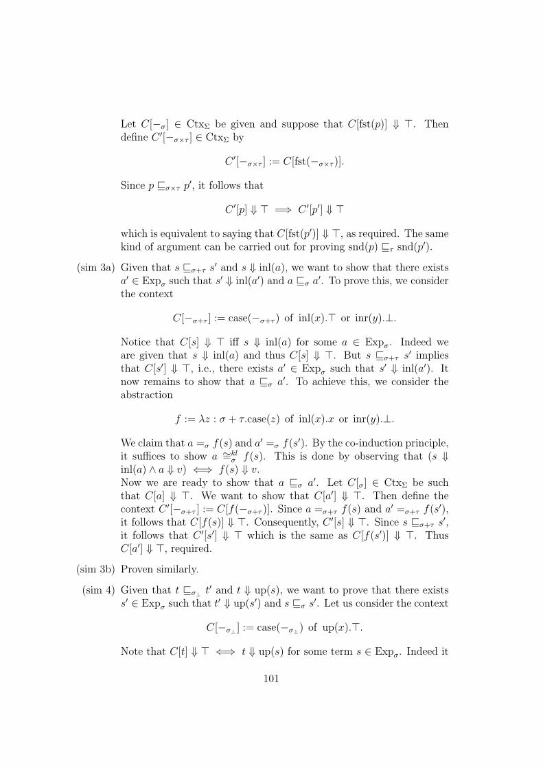
Let C[−σ] ∈ CtxΣ be given and suppose that C[fst(p)] ⇓ >. Thendefine C ′[−σ×τ ] ∈ CtxΣ by

C ′[−σ×τ ] := C[fst(−σ×τ )].

Since p vσ×τ p′, it follows that

C ′[p] ⇓ > =⇒ C ′[p′] ⇓ >

which is equivalent to saying that C[fst(p′)] ⇓ >, as required. The samekind of argument can be carried out for proving snd(p) vτ snd(p′).

(sim 3a) Given that s vσ+τ s′ and s ⇓ inl(a), we want to show that there existsa′ ∈ Expσ such that s′ ⇓ inl(a′) and a vσ a′. To prove this, we considerthe context

C[−σ+τ ] := case(−σ+τ ) of inl(x).> or inr(y).⊥.

Notice that C[s] ⇓ > iff s ⇓ inl(a) for some a ∈ Expσ. Indeed weare given that s ⇓ inl(a) and thus C[s] ⇓ >. But s vσ+τ s′ impliesthat C[s′] ⇓ >, i.e., there exists a′ ∈ Expσ such that s′ ⇓ inl(a′). Itnow remains to show that a vσ a′. To achieve this, we consider theabstraction

f := λz : σ + τ.case(z) of inl(x).x or inr(y).⊥.

We claim that a =σ f(s) and a′ =σ f(s′). By the co-induction principle,it suffices to show a ∼=kl

σ f(s). This is done by observing that (s ⇓inl(a) ∧ a ⇓ v) ⇐⇒ f(s) ⇓ v.Now we are ready to show that a vσ a′. Let C[σ] ∈ CtxΣ be suchthat C[a] ⇓ >. We want to show that C[a′] ⇓ >. Then define thecontext C ′[−σ+τ ] := C[f(−σ+τ )]. Since a =σ+τ f(s) and a′ =σ+τ f(s′),it follows that C[f(s)] ⇓ >. Consequently, C ′[s] ⇓ >. Since s vσ+τ s′,it follows that C ′[s′] ⇓ > which is the same as C[f(s′)] ⇓ >. ThusC[a′] ⇓ >, required.

(sim 3b) Proven similarly.

(sim 4) Given that t vσ⊥ t′ and t ⇓ up(s), we want to prove that there existss′ ∈ Expσ such that t′ ⇓ up(s′) and s vσ s′. Let us consider the context

C[−σ⊥ ] := case(−σ⊥) of up(x).>.

Note that C[t] ⇓ > ⇐⇒ t ⇓ up(s) for some term s ∈ Expσ. Indeed it

101

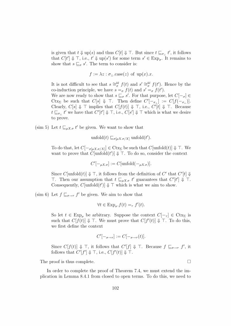
is given that t ⇓ up(s) and thus C[t] ⇓ >. But since t vσ⊥ t′, it followsthat C[t′] ⇓ >, i.e., t′ ⇓ up(s′) for some term s′ ∈ Expσ. It remains toshow that s vσ s′. The term to consider is:

f := λz : σ⊥.case(z) of up(x).x.

It is not difficult to see that s ∼=klσ f(t) and s′ ∼=kl

σ f(t′). Hence by theco-induction principle, we have s =σ f(t) and s′ =σ f(t′).We are now ready to show that s vσ s′. For that purpose, let C[−σ] ∈CtxΣ be such that C[s] ⇓ >. Then define C ′[−σ⊥ ] := C[f(−σ⊥)].Clearly, C[s] ⇓ > implies that C[f(t)] ⇓ >, i.e., C ′[t] ⇓ >. Becauset vσ⊥ t′ we have that C ′[t′] ⇓ >, i.e., C[s′] ⇓ > which is what we desireto prove.

(sim 5) Let t vµX.σ t′ be given. We want to show that

unfold(t) vσ[µX.σ/X] unfold(t′).

To do that, let C[−σ[µX.σ/X]] ∈ CtxΣ be such that C[unfold(t)] ⇓ >. Wewant to prove that C[unfold(t′)] ⇓ >. To do so, consider the context

C ′[−µX.σ] := C[unfold(−µX.σ)].

Since C[unfold(t)] ⇓ >, it follows from the definition of C ′ that C ′[t] ⇓>. Then our assumption that t vµX.σ t′ guarantees that C ′[t′] ⇓ >.Consequently, C[unfold(t′)] ⇓ > which is what we aim to show.

(sim 6) Let f vσ→τ f ′ be given. We aim to show that

∀t ∈ Expσ.f(t) =τ f ′(t).

So let t ∈ Expσ be arbitrary. Suppose the context C[−τ ] ∈ CtxΣ issuch that C[f(t)] ⇓ >. We must prove that C[f ′(t)] ⇓ >. To do this,we first define the context

C ′[−σ→τ ] := C[−σ→τ (t)].

Since C[f(t)] ⇓ >, it follows that C ′[f ] ⇓ >. Because f vσ→τ f ′, itfollows that C ′[f ′] ⇓ >, i.e., C[f ′(t)] ⇓ >.

The proof is thus complete.

In order to complete the proof of Theorem 7.4, we must extend the im-plication in Lemma 8.4.1 from closed to open terms. To do this, we need to

102

verify that the substitutivity property holds for v, i.e.,

Lemma 8.4.2. If Γ, x : σ ` s vτ s′, then it holds that

Γ ` s[t/x] vτ s′[t/x]

for every t ∈ Expσ(Γ).

Proof. We first claim that

Γ, x : σ ` s vτ s′ =⇒ Γ ` (λx.s)t vτ (λx.s′)t.

To prove this claim, let C[−τ ] ∈ CtxΣ(Γ) be such that C[(λx.s)t] ⇓ >. Nowdefine the context C ′[−τ ] := C[(λx.−τ )t]. Clearly, C ′[s] ⇓ > =⇒ C ′[t] ⇓ >,i.e., C[(λx.s)t] ⇓ >. Hence Γ ` (λx.s)t vτ (λx.s′)t. But since Γ ` s[t/x] vkl

τ

(λx.s′)t and Γ ` (λx.s′)t vklτ s′[t/x], it then follows from the co-induction

principle that Γ ` s[t/x] vτ (λx.s)t and Γ ` (λx.s′)t vτ s′[t/x]. By thetransitivity of vτ , we have that Γ ` s[t/x] vτ s′[t/x].

We are now ready to extend Lemma 8.4.1 from closed terms to openterms.

Lemma 8.4.3. For all Γ, σ, s, t,

Γ ` s vσ t =⇒ Γ ` s σ t.

Proof. Suppose that Γ ≡ x1 : σ1, . . . , x : σn ` s vσ t holds. For anysi ∈ Expσi

(i = 1, . . . , n), by applying Lemma 8.4.2 repeatedly, we get:

s[~s/~x] vσ t[~s/~x]

and since ∅ ` s vσ t implies ∅ ` s σ t, we have that:

s[~s/~x] σ t[~s/~x].

Thus by definition of , it follows that

Γ ` s σ t.

Thus the converse of Corollary 8.3.2 holds and we have completed theproof of Theorem 7.4.

103

8.5 Appendix

In this appendix, we record the proofs of Lemmas 8.2.1 and 8.2.2.

Proof of Lemma 8.2.1(1).We aim to prove that:If Γ ` t ∗σ t′ and Γ ` t′ σ t′′, then Γ ` t ∗σ t′′.We prove this by induction on the derivation of Γ ` t ∗σ t′.

(1) (∗ var)Given that Γ′, x : σ ` x ∗σ t′ and Γ′, x : σ ` t′ σ t′′, we must provethat Γ′, x : σ ` x ∗σ t′′. From (∗ var), Γ′, x : σ ` x ∗σ t′ holds only ifΓ′, x : σ ` x σ t′. It follows from Proposition 7.4.1(2) that

(Γ′, x : σ ` x σ t′ ∧ Γ′, x : σ ` t′ σ t′′) =⇒ Γ′, x : σ ` x σ t′′.

Then the required result follows from the axiom (∗ var)

Γ′, x : σ ` x ∗σ t′′(if Γ′, x : σ ` x t′′).

(2) (∗ abs)Given that Γ ` λx.s ∗σ→τ t′ and Γ ` t′ σ→τ t′′, we must show thatΓ ` λx.s ∗σ→τ t′′. The induction hypothesis asserts that Γ, x : σ `s ∗τ s′. From the inference rule (∗ abs), Γ ` λx.s ∗σ→τ t′ providedΓ ` λx.s′ ∗σ→τ t′ holds. By Proposition 7.4.1(2), we have

(Γ ` λx.s′ σ→τ t′ ∧ Γ ` t′ σ→τ t′′) =⇒ Γ ` λx.s′ σ→τ t′′.

The required result then follows from the inference rule (∗ abs)

Γ, x : σ ` s ∗τ s′

Γ ` λx.s ∗σ→τ t′′(if Γ ` λx.s′ σ→τ t′′).

(3) (∗ app)Given that Γ ` f(s) ∗τ t′ and Γ ` t′ τ t′′, we must show thatΓ ` f(s) ∗τ t′′. The induction hypothesis asserts that Γ ` f ∗σ→τ f ′

and Γ ` s ∗σ s′ for some f ′ and s′. Note that Γ ` f(s) ∗σ t′ holdsprovided Γ ` f ′(s′) τ t′. By Proposition 7.4.1(2), it then follows that

(Γ ` f ′(s′) τ t′ ∧ Γ ` t′ τ t′′) =⇒ Γ ` f ′(s′) τ t′′.

104

The required result then follows from the inference rule (∗ app)

Γ ` f ∗σ→τ f ′ Γ ` s ∗σ s′

Γ ` f(s) ∗τ t′′(if Γ ` f ′(s′) τ t′′).

(4) (∗ pair)Given that Γ ` (s, t) ∗σ×τ p′ and Γ ` t′ σ×τ p′′, we must show thatΓ ` (s, t) ∗σ×τ p′′. The induction hypothesis asserts that Γ ` s ∗σ s′

and Γ ` t ∗τ t′ for some terms s′ and t′. Also Γ ` (s, t) ∗σ×τ p′ holdsprovided Γ ` (s′, t′) σ×τ p′. By Proposition 7.4.1(2), it follows that

(Γ ` (s′, t′) σ×τ p′ ∧ Γ ` p′ σ×τ p′′) =⇒ Γ ` (s′, t′) σ×τ p′′.

The required result then follows from the rule (∗ pair)

Γ ` s ∗σ s′ Γ ` t ∗τ t′

Γ ` (s, t) ∗σ×τ p′′(if Γ ` (s′, t′) σ×τ p′′).

(5) (∗ fst, snd)Given that Γ ` fst(p) ∗σ t′ and Γ ` t′ σ t′′, we must show thatΓ ` fst(p) ∗σ t′′. The induction hypothesis asserts that Γ ` p ∗σ×τ p′

for some term p′. Note that Γ ` fst(p) ∗σ t′ holds provided Γ `fst(p′) σ t′. By Proposition 7.4.1(2), it follows that

(Γ ` fst(p′) σ t′ ∧ Γ ` t′ σ t′′) =⇒ Γ ` fst(p′) σ t′′.

The required result then follows from the rule (∗ fst)

Γ ` p ∗σ×τ p′

Γ ` fst(p) ∗σ t′′(if Γ ` fst(p′) σ t′′).

Similarly, the case holds for (∗ snd).

(6) (∗ inl, inr)Given that Γ ` inl(s) ∗σ+τ t′ and Γ ` t′ σ+τ t′′, we must showthat Γ ` inl(s) ∗σ+τ t′′. The induction hypothesis asserts that Γ `s ∗σ s′ for some s′. Note that Γ ` inl(s) ∗σ+τ t′ holds providedΓ ` inl(s′) σ+τ t′. By Proposition 7.4.1(2), it follows that

(Γ ` inl(s′) σ+τ t′ ∧ Γ ` t′ σ+τ ) =⇒ Γ ` inl(s′) σ+τ t′′.

105

The required result then follows from the inference rule (∗ inl)

Γ ` s ∗σ s′

Γ ` inl(s) ∗σ+τ t′′(if Γ ` inl(s′) σ+τ t′′).

Similarly, the case for (∗ inr) holds.

(7) (∗ case)Given that Γ ` case(s) of inl(x).t1 or inr(y).t2 ∗ρ t′ and Γ ` t′ ρ t′′,we must show that Γ ` case(s) of inl(x).t1 or inr(y).t2 ∗ρ t′′. Theinduction hypothesis asserts that Γ ` s ∗σ+τ s′, Γ, x : σ ` t1 ∗ρt′1 and Γ, y : τ ` t2 ∗ρ t′2 for some terms s′, t′1, t

′2. Note that Γ `

case(s) of inl(x).t1 or inr(y).t2 ∗ρ t′ holds provided

Γ ` case(s′) of inl(x).t′1 or inr(y).t′2 ρ t′.

By Proposition 7.4.1(2), it follows that(Γ ` case(s′) of inl(x).t′1 or inr(y).t′2 ρ t′ ∧ Γ ` t′ ρ t′′) =⇒Γ ` case(s′) of inl(x).t′1 or inr(y).t′2 ρ t′′.

Using the inference rule (∗ case), the required result:

Γ ` s ∗σ+τ s′ Γ, x : σ ` t1 : ρ Γ, y : τ ` t2 : ρΓ ` case(s) of inl(x).t1 or inr(y).t2 ∗ρ t′′

(if Γ ` case(s′) of inl(x).t′1 or inr(y).t′2 ρ t′′).

(8) (∗ up)Given that Γ ` up(s) ∗σ⊥ t′ and Γ ` t′ σ⊥ t′′, we want to show thatΓ ` up(s) ∗σ⊥ t′′. The induction hypothesis asserts that Γ ` s ∗σ s′ forsome s′. Note that Γ ` up(s) ∗σ⊥ t′ holds provided Γ ` up(s′) σ⊥ t′′.By Proposition 7.4.1(2), it follows that

(Γ ` up(s′) σ⊥ t′ ∧ Γ ` t′ σ⊥ t′′) =⇒ Γ ` up(s′) σ⊥ t′′.

The required result then follows from the inference rule (∗ up)

Γ ` s ∗σ s′

Γ ` up(s) ∗σ⊥ t′′(if Γ ` up(s′) σ⊥ t′′).

(9) (∗ case up)Given that Γ ` case(s) of up(x).r ∗ρ t′ and Γ ` t′ ∗ρ t′′, we mustshow that Γ ` case(s) of up(x).r ∗ρ t′′. The induction hypothesisasserts that Γ ` s ∗σ⊥ s′ and Γ, x : σ ` r ∗ρ r′ for some terms s′

106

and r′. Note that Γ ` case(s) of up(x).r ∗ρ t′ holds provided thatΓ ` case(s′) of up(x).r′ ρ t′. By Proposition 7.4.1(2), it follows that

(Γ ` case(s′) of up(x).r′ ρ t′ ∧ Γ ` t′ ρ t′′) =⇒Γ ` case(s′) of up(x).r′ ρ t′′.

The required result follows from the inference rule (∗ case up)

Γ ` s ∗σ⊥ s′ Γ, x : σ ` r ∗ρ r′

Γ ` case(s) of up(x).r ∗ρ t′′(if Γ ` case(s′) of up(x).r ρ t′′).

(10) (∗ unfold)Given that Γ ` unfold(s) ∗σ[µX.σ/X] t′ and Γ ` t′ ∗σ[µX.σ/X] t′′, we must

show that Γ ` unfold(s) ∗σ[µX.σ/X] t′′. The induction hypothesis asserts

that Γ ` s ∗µX.σ s′ for some s′. Note that Γ ` unfold(s) ∗σ[µX.σ/X] t′

holds provided Γ ` unfold(s′) σ[µX.σ/X] t′. By Proposition 7.4.1(2), itfollows that

(Γ ` unfold(s′) µX.σ t′ ∧ Γ ` t′ µX.σ t′′) =⇒ Γ ` unfold(s′) µX.σ t′′.

The required result then follows from the inference rule (∗ unfold)

Γ ` s ∗µX.σ s′

Γ ` unfold(s) ∗σ[µX.σ/X] t′′(if Γ ` unfold(s′) σ[µX.σ/X] t′′).

(11) (∗ fold)Given that Γ ` fold(s) ∗µX.σ t′ and Γ ` t′ ∗µX.σ t′′, we must show thatΓ ` r′ ∗µX.σ t′′. The induction hypothesis asserts that Γ ` s ∗σ[µX.σ/X]

s′ for some term s′. Note that Γ ` t′ ∗µX.σ t′ holds provided Γ `fold(s′) µX.σ t′. By Proposition 7.4.1(2), it then follows that

(Γ ` fold(s′) µX.σ t′ ∧ Γ ` t′ µX.σ t′′) =⇒ Γ ` fold(s′) µX.σ t′′.

The required result then follows from the inference rule (∗ fold)

Γ ` s ∗σ[µX.σ/X] s′

Γ ` fold(s) ∗µX.σ t′′(if Γ ` fold(s′) σ[µX.σ/X] t′′).

The proof by induction is now complete.

Proof of Lemma 8.2.1(2).We aim to prove that:If Γ ` t : σ, then Γ ` t ∗σ t.The proof proceeds by induction on the derivation of Γ ` t : σ.

107

(1) (` var)Given that Γ′, x : σ ` x : σ, we must show that Γ′, x : σ ` x ∗σ x. ByProposition 7.4.1(1), we have Γ′, x : σ ` x σ x. Hence, by the axiom(∗ var), we have Γ′, x : σ ` x ∗σ x.

(2) (` abs)Given that Γ ` λx.t : σ → τ , we must show that Γ ` λx.t ∗σ→τ λx.t.The induction hypothesis asserts that Γ, x : σ ` t ∗τ t. Note thatΓ ` λx.t λx.t by Proposition 7.4.1(1). Hence, by the inference rule(∗ abs), we have Γ ` λx.t ∗σ→τ λx.t.

(3) (` app)Given that Γ ` f(s) : τ , we must show that Γ ` f(s) ∗τ f(s). Theinduction hypothesis asserts that Γ ` f ∗σ→τ f and Γ ` s ∗σ s. Notethat Γ ` f(s) τ f(s) by Proposition 7.4.1(1). Hence, by the inferencerule (∗ app), we have Γ ` f(s) ∗τ f(s).

(4) (` pair)Given that Γ ` (s, t) : σ × τ , we must show that Γ ` (s, t) ∗σ×τ (s, t).The induction hypothesis asserts that Γ ` s ∗σ s and Γ ` t ∗τ t.By Proposition 7.4.1(1), we have Γ ` (s, t) σ×τ (s, t). Hence, by theinference rule (∗ pair), we have Γ ` (s, t) ∗σ×τ (s, t).

(5) (` fst, snd)Given that Γ ` fst(p) : σ, we must show that Γ ` fst(p) ∗σ fst(p).The induction hypothesis asserts that Γ ` p ∗σ×τ p. By Proposition7.4.1(1), it follows that Γ ` fst(p) σ fst(p). Hence, by the inferencerule (∗ fst), we have Γ ` fst(p) ∗σ fst(p).Similarly, the case (` snd) holds.

(6) (` up)Given that Γ ` up(t) : σ⊥, we must show that Γ ` up(t) ∗σ⊥ up(t).The induction hypothesis asserts that Γ ` t ∗σ t. Note that Γ `up(t) σ⊥ up(t) by Proposition 7.4.1(1). Hence, by the inference rule(∗ up), we have Γ ` up(t) ∗σ⊥ up(t).

(7) (` case up)Given that Γ ` case(s) of up(x).t : ρ, we must show thatΓ ` case(s) of up(x).t ∗ρ case(s) of up(x).t. The induction hypoth-esis asserts that Γ ` s ∗σ⊥ s and Γ, x : σ ` t ∗ρ t. Note thatΓ ` case(s) of up(x).t ρ case(s) of up(x).t by Proposition 7.4.1(1).Hence, by the inference rule (∗ case up), we haveΓ ` case(s) of up(x).t ∗ρ case(s) of up(x).t.

108

(8) (` inl, inr)Given that Γ ` inl(t) : σ + τ , we must show that Γ ` inl(t) ∗σ+τ

inl(t). The induction hypothesis asserts that Γ ` t ∗σ t. Note thatΓ ` inl(t) σ+τ inl(t) by Proposition 7.4.1(1). Hence, by the inferencerule (∗ inl), we have Γ ` inl(t) ∗σ+τ inl(t).Similarly, the case (` inr) holds.

(9) (` case)Given that Γ ` case(s) of inl(x).t1 or inr(y).t2 : ρ, we must show thatΓ ` case(s) of inl(x).t1 or inr(y).t2 ∗ρ case(s) of inl(x).t1 or inr(y).t2.The induction hypothesis asserts that Γ ` s ∗σ+τ s, Γ, x : σ ` t1 ∗ρ t1and Γ, y : τ ` t2 ∗ρ t2. Note that Γ ` case(s) of inl(x).t1 or inr(y).t2 ρcase(s) of inl(x).t1 or inr(y).t2 by Proposition 7.4.1(1). Hence, by theinference rule (∗ case), we have Γ ` case(s) of inl(x).t1 or inr(y).t2 ∗ρcase(s) of inl(x).t1 or inr(y).t2.

(10) (` unfold)Given that Γ ` unfold(t) : σ[µX.σ/X], we must show thatΓ ` unfold(t) ∗σ[µX.σ/X] unfold(t). The induction hypothesis asserts

that Γ ` t ∗µX.σ t. Note that Γ ` unfold(t) σ[µX.σ/X] unfold(t)

by Proposition 7.4.1(1). Hence, by the inference rule (∗ unfold), wehave Γ ` unfold(t) ∗σ[µX.σ/X] unfold(t).

(10) (` fold)Given that Γ ` fold(t) : µX.σ, we must show that Γ ` fold(t) ∗µX.σ

fold(t). The induction hypothesis asserts that Γ ` t ∗σ[µX.σ/X] t. Note

that Γ ` fold(t) µX.σ fold(t) by Proposition 7.4.1(1). Hence, by theinference rule (∗ fold), we have Γ ` fold(t) ∗µX.σ fold(t).

Proof of Lemma 8.2.1. (3)We aim to prove that:If Γ ` t σ t′, then Γ ` t ∗σ t′.Note that by (2), Γ ` t ∗σ t holds whenever Γ ` t : σ. Thus by (1),(Γ ` t ∗σ t ∧ Γ ` t σ t′) =⇒ Γ ` t ∗σ t′.

Proof of Lemma 8.2.1. (4)We aim to prove that:If Γ ` t ∗σ t′ and Γ, x : σ ` s ∗τ s′, then Γ ` s[t/x] ∗τ s′[t′/x].We prove this by induction on the derivation of Γ, x : σ ` s ∗σ s′.

109

(1) (∗ var)Case 1: Γ, x : σ ` x ∗σ s′.Given that Γ ` t ∗σ t′ and Γ, x : σ ` x ∗σ s′, we must show that

Γ ` t ∗σ s′[t′/x].

Firstly, from the axiom (∗ var), one notes that Γ, x : σ ` x ∗σ s′

holds only if Γ, x : σ ` x σ s′. Secondly, by Proposition 7.4.1(1),it holds that Γ ` t′ σ t′. It then follows from Lemma 7.4.2 thatΓ ` t′ σ s′[t′/x]. By Lemma 8.2.1(1), we have

(Γ ` t ∗σ t′ ∧ Γ ` t′ σ s′[t′/x]) =⇒ Γ ` t ∗σ s′[t′/x].

Case 2: Γ, x : σ ` y ∗τ s′ where y is a term variable distinct from x.Given that Γ ` t ∗σ t′ and Γ, x : σ ` y ∗τ s′, we must prove that

Γ ` y ∗τ s′[t′/x].

From the axiom (∗ var), one notes that Γ, x : σ ` y ∗τ s′ holds onlyif Γ, x : σ ` y τ s′. By Proposition 7.4.1(1), it holds that Γ ` t′ σ t′.Thus, by Lemma 7.4.2, it follows that Γ ` y τ s′[t′/x]. Lemma8.2.1(2) ensures that Γ ` y ∗τ y always holds. By Lemma 8.2.1(1), wehave

(Γ ` y ∗τ y ∧ Γ ` y τ s′[t′/x]) =⇒ Γ ` y ∗τ s′[t′/x].

(2) (∗ abs)Given that Γ ` t ∗σ t′ and Γ, x : σ ` λy.r ∗ρ→τ s′, we must show that

Γ ` λy.r[t/x] ∗ρ→τ s′[t′/x].

Since Γ ` λy.r ∗ρ→τ s′, it follows from the inference rule (∗ abs)that Γ, y : ρ ` r ∗τ r′ for some term r′ with Γ ` λx.r′ ρ→τ s′. Theinduction hypothesis then asserts that Γ, y : ρ ` r[t/x] ∗τ r′[t′/x].Note that one always has Γ ` t′ σ t′ by Proposition 7.4.1(1). Thus,by Lemma 7.4.2(2), we have

(Γ, x : σ ` λy.r′ ρ→τ s′ ∧ Γ ` t t′) =⇒ Γ ` λy.r′[t′/x] ρ→σ s′[t′/x].

Since Γ, y : ρ ` r[t/x] ∗τ r′[t′/x] and Γ ` λy.r′[t′/x] ρ→τ s′[t′/x], it

110

follows from the inference rule (∗ abs) that

Γ ` λy.r[t/x] ∗ρ→τ s′[t′/x].

(3) (∗ app)Given that Γ ` t ∗σ t′ and Γ, x : σ ` f(r) ∗τ s′, we must show that

Γ ` f(r)[t/x] ∗τ s′[t′/x].

Since Γ ` f(r) ∗τ s′, it follows from the inference rule (∗ app) thatΓ, x : σ ` f ∗ρ→τ f ′ and Γ, x : σ ` r ∗ρ r′ for some terms f ′ andr′ with Γ, x : σ ` f ′(r′) τ s′. The induction hypothesis asserts thatΓ ` f [t/x] ∗ρ→τ f ′[t′/x] and Γ ` r[t/x] ∗τ r′[t′/x]. Since Γ ` t′ t′

by Proposition 7.4.1(1) and Γ, x : σ ` f ′(r′) τ s′, it follows fromLemma 7.4.2 that Γ ` f ′(r′)[t′/x] τ s′[t′/x]. Thus it follows from theinference rule (∗ app) that

Γ ` f(r)[t/x] ∗τ s′[t′/x].

(4) (∗ pair)Given that Γ ` t ∗σ t′ and Γ, x : σ ` (m1, m2) ∗τ1×τ2

s′, we must showthat

Γ ` (m1, m2)[t/x] ∗τ1×τ2s′[t′/x].

Since Γ, x : σ ` (m1, m2) ∗τ1×τ2s′, it follows from the inference rule

(∗ pair) that Γ, x : σ ` m1 ∗τ1 m′1 and Γ, x : σ ` m2 ∗τ2 m′2 for someterms m′1 and m′2 with Γ, x : σ ` (m′1, m

′2) τ1×τ2

s′. On one hand, theinduction hypothesis then asserts that Γ ` m1[t/x] ∗τ1 m′1[t

′/x] andΓ ` m2[t/x] ∗τ2 m′2[t

′/x]. On the other hand, since Γ ` t′ σ t′ alwaysholds by Proposition 7.4.1, it follows that Γ ` (m′1, m

′2)[t′/x] τ1×τ2

s′[t′/x].Finally, it follows from the inference rule (∗ pair) that

Γ ` (m1, m2)[t/x] ∗τ1×τ2s′[t′/x].

(5) (∗ fst, snd)Given that Γ ` t ∗σ t′ and Γ, x : σ ` fst(p) ∗τ1 s′, we must show that

Γ ` fst(p)[t/x] ∗τ1 s′[t′/x].

Since Γ, x : σ ` fst(p) ∗τ1 s′, it follows from the inference rule thatΓ, x : σ ` p ∗τ1×τ2

p′ for some term p′ with Γ, x : σ ` fst(p′) τ1 s′.On one hand, the induction hypothesis then asserts that Γ ` p[t/x] ∗τ1

111

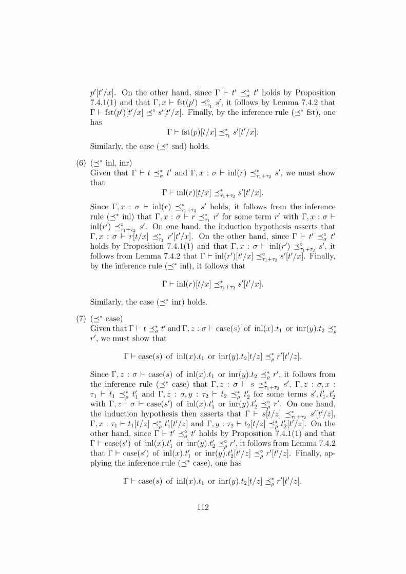
p′[t′/x]. On the other hand, since Γ ` t′ σ t′ holds by Proposition7.4.1(1) and that Γ, x ` fst(p′) τ1 s′, it follows by Lemma 7.4.2 thatΓ ` fst(p′)[t′/x] s′[t′/x]. Finally, by the inference rule (∗ fst), onehas

Γ ` fst(p)[t/x] ∗τ1 s′[t′/x].

Similarly, the case (∗ snd) holds.

(6) (∗ inl, inr)Given that Γ ` t ∗σ t′ and Γ, x : σ ` inl(r) ∗τ1+τ2

s′, we must showthat

Γ ` inl(r)[t/x] ∗τ1+τ2s′[t′/x].

Since Γ, x : σ ` inl(r) ∗τ1+τ2s′ holds, it follows from the inference

rule (∗ inl) that Γ, x : σ ` r ∗τ1 r′ for some term r′ with Γ, x : σ `inl(r′) τ1+τ2

s′. On one hand, the induction hypothesis asserts thatΓ, x : σ ` r[t/x] ∗τ1 r′[t′/x]. On the other hand, since Γ ` t′ σ t′

holds by Proposition 7.4.1(1) and that Γ, x : σ ` inl(r′) τ1+τ2s′, it

follows from Lemma 7.4.2 that Γ ` inl(r′)[t′/x] τ1+τ2s′[t′/x]. Finally,

by the inference rule (∗ inl), it follows that

Γ ` inl(r)[t/x] ∗τ1+τ2s′[t′/x].

Similarly, the case (∗ inr) holds.

(7) (∗ case)Given that Γ ` t ∗σ t′ and Γ, z : σ ` case(s) of inl(x).t1 or inr(y).t2 ∗ρr′, we must show that

Γ ` case(s) of inl(x).t1 or inr(y).t2[t/z] ∗ρ r′[t′/z].

Since Γ, z : σ ` case(s) of inl(x).t1 or inr(y).t2 ∗ρ r′, it follows fromthe inference rule (∗ case) that Γ, z : σ ` s ∗τ1+τ2

s′, Γ, z : σ, x :τ1 ` t1 ∗ρ t′1 and Γ, z : σ, y : τ2 ` t2 ∗ρ t′2 for some terms s′, t′1, t

′2

with Γ, z : σ ` case(s′) of inl(x).t′1 or inr(y).t′2 ρ r′. On one hand,the induction hypothesis then asserts that Γ ` s[t/z] ∗τ1+τ2

s′[t′/z],Γ, x : τ1 ` t1[t/z] ∗ρ t′1[t

′/z] and Γ, y : τ2 ` t2[t/z] ∗ρ t′2[t′/z]. On the

other hand, since Γ ` t′ σ t′ holds by Proposition 7.4.1(1) and thatΓ ` case(s′) of inl(x).t′1 or inr(y).t′2 ρ r′, it follows from Lemma 7.4.2that Γ ` case(s′) of inl(x).t′1 or inr(y).t′2[t

′/z] ρ r′[t′/z]. Finally, ap-plying the inference rule (∗ case), one has

Γ ` case(s) of inl(x).t1 or inr(y).t2[t/z] ∗ρ r′[t′/z].

112

(8) (∗ up)Given that Γ ` t ∗σ t′ and Γ, x : σ ` up(r) ∗τ⊥ s′, we must show that

Γ ` up(r)[t/x] ∗τ⊥ s′[t′/x].

Since Γ, x : σ ` up(r) ∗τ⊥ s′ holds, it follows from the inference rulethat Γ, x : σ ` r ∗τ r′ for some term r′ with Γ, x : σ ` up(r′) τ s′. Onone hand, the induction hypothesis asserts that Γ ` r[t/x] ∗τ⊥ r′[t′/x].On the other hand, since Γ ` t′ σ t′ by Proposition 7.4.1(1) and thatΓ ` up(r′) s′, it follows from Lemma 7.4.2 that Γ ` up(r′)[t′/x] τ⊥s′[t′/x]. Finally, by the inference rule (∗ up), we have

Γ ` up(r)[t/x] ∗τ⊥ s′[t′/x].

(9) (∗ case up)Given that Γ ` t ∗σ t′ and Γ, z : σ ` case(s) of up(x).u ∗ρ r′, we mustshow that

Γ ` case(s) of up(x).u[t/x] ∗ρ r′[t′/z].

Since Γ, z : σ ` case(s) of up(x).u ∗ρ r′, it follows from the inferencerule (∗ case up) that Γ, z : σ ` s ∗τ⊥ s′ and Γ, z : σ, x : τ ` u ∗ρ u′ forsome s′ and u′ such that Γ, z : σ ` case(s′) of up(x).u′ ρ r′. On onehand, the induction hypothesis asserts that Γ ` s[t/z] ∗τ⊥ s′[t′/z] andΓ, x : τ ` u[t/z] ∗ρ u′[t′/z]. On the other hand, since Γ ` t′ σ t′ holdsby Proposition 7.4.1(1) and that Γ, z : σ ` case(s′) of up(x).u′ ρ r′,it follows from Lemma 7.4.2 that Γ ` case(s′) of up(x).u′[t′/x] ρr′[t′/x]. Finally, by the inference rule (∗ case up), it follows that

Γ ` case(s) of up(x).u[t/x] ∗ρ r′[t′/x].

(10) (∗ unfold)Given that Γ ` t ∗σ t′ and Γ, x : σ ` unfold(r) ∗τ [µX.τ/X] s′, we mustshow that

Γ ` unfold(r)[t/x] ∗τ [µX.τ/X] s′[t′/x].

Since Γ, x : σ ` unfold(r) ∗τ [µX.τ/X] s′ holds, it follows from the in-

ference rule (∗ unfold) that Γ, x : σ ` r ∗µX.τ r′ for some termr′ with Γ, x : σ ` unfold(r′) τµX.τ/X] s′. On one hand, the induc-

tion hypothesis asserts that Γ ` r[t/x] ∗µX.τ r′[t′/x]. On the otherhand, since Γ ` t′ σ t′ by Proposition 7.4.1(1) and that Γ, x :σ ` unfold(r′) τ [µX.τ/X] s′, it follows from Lemma 7.4.2 that Γ `unfold(r′)[t′/x] τ [µX.τ/X] s′[t′/x]. Finally, by the inference rule (∗

113

unfold), we have

Γ ` unfold(r)[t/x] ∗τ [µX.τ/X] s′[t′/x].

(11) (∗ fold)Given that Γ ` t ∗σ t′ and Γ, x : σ ` fold(r) ∗µX.τ s′, we must showthat

Γ ` fold(r)[t/x] ∗µX.τ s′[t′/x].

Since Γ, x : σ ` fold(r) ∗µX.τ ] s′ holds, it follows from the inference

rule (∗ unfold) that Γ, x : σ ` r ∗τ [µX.τ/X] r′ for some term r′ with

Γ, x : σ ` fold(r′) µX.τ s′. On one hand, the induction hypothesisasserts that Γ ` r[t/x] ∗τ [µX.τ/X] r′[t′/x]. On the other hand, since Γ `t′ σ t′ by Proposition 7.4.1(1) and that Γ, x : σ ` fold(r′) µX.τ s′, itfollows from Lemma 7.4.2 that Γ ` fold(r′)[t′/x] µX.τ s′[t′/x]. Finally,by the inference rule (∗ unfold), we have

Γ ` fold(r)[t/x] ∗µX.τ s′[t′/x].

The proof is now complete.

Proof of Proposition 8.2.2.We aim to show that:If Γ ` s ∗σ t and s ⇓ v, then Γ ` v ∗σ t.We proceed by induction on the derivation of s ⇓ v.

(1) (⇓ can) Trivial.

(2) (⇓ app)Given that ∅ ` f(r) ∗τ t and f(r) ⇓ v, we must show that

∅ ` f(r) ∗τ v.

Since ∅ ` f(r) ∗τ t, it follows from the inference rule (∗ app) that∅ ` f ∗σ→τ f ′ and ∅ ` r ∗τ r′ with f ′(r′) τ t. Note that f(r) ⇓ vis derived from f ⇓ λx.s and s[r/x] ⇓ v. By the induction hypothesis,it follows that ∅ ` λx.s ∗σ→τ f ′. From the inference rule (∗ abs), itmust be that x : σ ` s ∗τ s′ for some term s′ with Γ ` λx.s′ σ→τ f ′.Now applying Lemma 8.2.1(4), we have ∅ ` s[r/x] ∗τ s′[r′/x]. Since∅ ` s[r/x] ∗τ s′[r′/x] and s[r/x] ⇓ v, it follows from the inductionhypothesis that ∅ ` v ∗τ s′[r′/x]. Because is an FPC simulation andλx.s′ σ→τ f ′, it follows from (sim 3) that λx.s′(r′) τ f ′(r′). Note thatby definition of vkl, we always have s′[r′/x] vkl (λx.s′)(r′) and hence by

114

Proposition 7.5.1, s′[r′/x] τ (λx.s′)(r′). Thus, by transitivity, we have∅ ` s′[r′/x] τ t. Finally, since ∅ ` v ∗τ s′[r′/x] and ∅ ` s′[r′/x] τ t,it follows from Lemma 8.2.1(1) that ∅ ` v ∗τ t.

(3) (⇓ fst, snd) Given that ∅ ` fst(p) ∗σ t and fst(p) ⇓ v, we must showthat

∅ ` v ∗σ t.

Since ∅ ` fst(p) ∗σ t, it follows from the inference rule (∗ fst) that∅ ` p ∗σ×τ p′ for some term p′ with ∅ ` fst(p′) σ×τ t. Note thatfst(p) ⇓ v is derived from p ⇓ (m1, m2) and s ⇓ v. The inductionhypothesis then asserts that ∅ ` (m1, m2) ∗σ×τ p′. But from theinference rule (∗ pair), it must be that ∅ ` m1 ∗σ m′1 and ∅ ` m2 ∗τm′2 with ∅ ` (m′1, m

′2) σ×τ p′. By the induction hypothesis applied

to ∅ ` m1 ∗σ m′1 and s ⇓ v, we have ∅ ` v ∗σ m′1. Now since is an FPC simulation and (m′1, m

′2) σ×τ p′, it follows from (sim 4)

that fst(m′1, m′2) σ fst(p′). Note that by the definition of vkl, we

always have m′1 vklσ fst(m′1, m

′2). Hence by Proposition 7.5.1, it holds

that m′1 σ fst(m′1, m′2). Thus, by transitivity, we have ∅ ` m′1 σ t.

Finally, since ∅ ` v ∗σ m′1 and ∅ ` m1 σ t, it then follows fromLemma 8.2.1(1) that ∅ ` v ∗σ t.Similarly, the case (∗ snd) holds.

(4) (⇓ case inl)Given that ∅ ` case(s) of inl(x).t1 or inr(y).t2 ∗ρ t andcase(s) of inl(x).t1 or inr(y).t2 ⇓ v, we must show that ∅ ` v ∗ρ t.Since ∅ ` case(s) of inl(x).t1 or inr(y).t2 ∗ρ t holds, it follows from theinference rule (∗ case inl) that ∅ ` s ∗σ+τ s′ and x : σ ` t1 ∗ρ t′1 andy : τ ` t2 ∗ρ t′2 with ∅ ` case(s′) of inl(x).t′1 or inr(y).t′2 ρ t. Notethat for this case, the evaluation case(s) of inl(x).t1 or inr(y).t2 ⇓ vis derived from s ⇓ inl(a) and t1[a/x] ⇓ v. The induction hypothesisapplied to ∅ ` s ∗σ+τ s′ and s ⇓ inl(a) then asserts that ∅ ` inl(a) ∗σ+τ

s′. But this holds provided that ∅ ` a ∗σ a′ for some a′ with ∅ `inl(a′) σ+τ s′. Since is an FPC simulation and inl(a′) σ+τ s′, itfollows from (sim 5) that there is a′′ : σ such that s′ ⇓ inl(a′′) anda′ σ a′′. Note that by the definition of vkl, we have t′1[a

′′/x] vklρ

case(s′) of inl(x).t′1 or inr(y).t′2 and hence by Lemma 7.5.1, it holdsthat t′1[a

′′/x] ρ case(s′) of inl(x).t′1 or inr(y).t′2. Consequently, bytransitivity, we have t′1[a

′′/x] ρ t. Because ∅ ` a ∗σ a′ and ∅ `a′ σ a′′, by Lemma 8.2.1(1) it holds that ∅ ` a ∗σ a′′. Now sincex : σ ` t1 ∗ρ t′1, using Lemma 7.4.2 one deduces that ∅ ` t1[a/x] ∗ρt′1[a

′′/x]. Since t1[a/x] ⇓ v, the induction hypothesis then asserts that

115

∅ ` v ∗ρ t′1[a′′/x]. Finally, since ∅ ` t′1[a

′′/x] ρ t, it follows fromLemma 8.2.1(1) that ∅ ` v ∗ρ t.Similarly, the case (∗ inr) holds.

(5) (⇓ case up)Given that ∅ ` case(s) of up(x).r ∗ρ t and case(s) of up(x).r ⇓ v, wemust show that ∅ ` v ∗ρ t. Since ∅ ` case(s) of up(x).r ∗ρ t holds,it follows from the inference rule (∗ case up) that ∅ ` s ∗σ⊥ s′ andx : σ ` r ∗ρ r′ with ∅ ` case(s′) of up(x).r′ ρ t. Note that for thiscase, the evaluation case(s) of up(x).r ⇓ v is derived from s ⇓ up(a)and r[a/x] ⇓ v. The induction hypothesis applied to ∅ ` s ∗σ⊥ s′ ands ⇓ up(a) then asserts that ∅ ` up(a) ∗σ⊥ s′. But this holds providedthat ∅ ` a ∗σ a′ for some a′ with ∅ ` up(a′) σ⊥ s′. Since is anFPC simulation and up(a′) σ⊥ s′, it follows from (sim 5) that there isa′′ : σ such that s′ ⇓ up(a′′) and a′ σ a′′. Note that by the definitionof vkl, we have r′[a′′/x] vkl

ρ case(s′) of up(x).r′ and hence by Lemma7.5.1, it holds that r′[a′′/x] ρ case(s′) of up(x).r′. Consequently, bytransitivity, we have r′[a′′/x] ρ t. Because ∅ ` a ∗σ a′ and ∅ `a′ σ a′′, by Lemma 8.2.1(1) it holds that ∅ ` a ∗σ a′′. Now sincex : σ ` r ∗ρ r′, using Lemma 7.4.2 one deduces that ∅ ` r[a/x] ∗ρr′[a′′/x]. Since r[a/x] ⇓ v, the induction hypothesis then asserts that∅ ` v ∗ρ r′[a′′/x]. Finally, since ∅ ` r′[a′′/x] ρ t, it follows fromLemma 8.2.1(1) that ∅ ` v ∗ρ t.

(6) (⇓ unfold)Given that ∅ ` unfold(s) ∗τ [µX.τ/X] t and unfold(s) ⇓ v, we must showthat

∅ ` v ∗τ [µX.τ/X] t.

Since ∅ ` unfold(s) ∗τ [µX.τ/X] t holds, it follows from the inference rule

(∗ unfold) that ∅ ` s ∗µX.τ s′ for some s′ with ∅ ` unfold(s′) τ [µX.τ/X]

t. Note that unfold(s) ⇓ v derives from s ⇓ fold(r) and r ⇓ v. Since∅ ` s ∗µX.τ s′ and s ⇓ fold(r), the induction hypothesis then assertsthat ∅ ` fold(r) ∗µX.τ s′. But this holds provided that ∅ ` r ∗τ [µX.τ/X]

r′ for some term r′ with ∅ ` fold(r′) µX.τ s′. Now since is anFPC simulation and fold(r′) µX.τ s′, it follows from (sim 6) that∅ ` unfold(fold(r)) τ [µX.τ/X] unfold(s′). Note that by the definition

of vkl, one always has r′ vklτ [µX.τ/X] unfold(fold(r′)) and by Proposi-

tion 7.5.1, it holds that ∅ ` r′ τ [µX.τ/X] unfold(s′). Applying Lemma

8.2.1(1) to ∅ ` r ∗τ [µX.τ/X] r′ and ∅ ` r′ τ [µX.τ/X] unfold(s′), we have

∅ ` r ∗τ [µX.τ/X] unfold(s′). Since r ⇓ v, the induction hypothesis as-

116

serts that ∅ ` v ∗µX.τ unfold(s′). Finally, since ∅ ` unfold(s′) µX.τ t,it follows from Lemma 8.2.1(1) that ∅ ` v ∗τ [µX.τ/X] t.

The proof is now complete.

117

Part III

Operational Domain Theory forPCF

118

In this part, we present an operational domain theory and topology forthe language PCF. Rational chains and rational topology are dealt with inChapter 9. In Chapter 10, an operational notion of finiteness is introducedand studied. An SFP-structure for PCF types is derived in that same chapter.In Chapter 11, compactness is revisited. We see how compactness interactswith finiteness. Note that the materials on saturated sets and well-filteredsubspaces in Chapter 11 are new. In Chapter 12, reasoning principles devel-oped in Chapters 9, 10 and 11 are applied to establish program correctnessof some non-trivial PCF programs.

119

Chapter 9

Rational chains and rationaltopology

In this chapter, we show that rational chains are equivalent to programsdefined on the “vertical natural number” type ω. A crucial step in the devel-opment of an operational domain theory for PCF is to replace the directedsets by rational chains. With this replacement, several classical results gothrough smoothly. The highlight in this chapter is that the open sets of anytype (1) form a ‘rational’ topology and (2) are ‘rationally’ Scott-open.

9.1 Rationale for rational chains

In this section, we briefly discuss the need for using rational chains in thedevelopment of operational domain theory.

In pure PCF, there are types which fail to be chain complete because ofcomputability reasons. This fact is well-known and appears, for instance,in the work of Mason, Smith & Talcott [36]. For clarity, we present theargument here.

Proposition 9.1.1. In pure PCF, the contextual pre-order is not chain com-plete, i.e., there exist a type σ and a chain D ⊆ σ with no least upper bound.

Proof. Let φ : N → N be a non-computable function. For each k ∈ N, definethe program fk : Nat→ Nat as follows:

fk = if n ≤ k then φ(n) else ⊥.

Note that the subset D = fk|k ∈ N ⊆ (Nat → Nat) does not have a leastupper bound because the least upper bound, if it existed, would have beencontextually equivalent to φ.

120

Note that this example ‘disappears’ if we move from PCF to PCFΩ. How-ever, Dag Normann recently constructed an explicit example of a chain inPCF which does not have a least upper bound in PCFΩ but does have abound in PCF++. So, the least upper bound exists in some sense, and iscomputable, but not sequential. Therefore, PCFΩ is also not chain com-plete. However, PCF++

Ω is chain complete because it is equivalent to theScott model of PCF (see, for example, Theorem 5.3.4). Because of the sheercomplexity of its construction, Normann’s example is beyond the scope ofthis thesis. But the interested reader may find it, together with detailedexplanations, in Normann [39].

In view of the failure of chain completeness (with respect to contextualpreorder) in PCF and PCFΩ, we are forced to work with a restricted form ofchain completeness, i.e., rational chain completeness, cf. Pitts [41].

9.2 Rational continuity

We begin by making a simple but crucial observation.

Lemma 9.2.1. The sequence 0, 1, . . . , n, . . . in ω is a rational chain withleast upper bound ∞, and

l(∞) =⊔n

l(n) for every l ∈ (ω → σ).

Proof. n = succ(n)(⊥) and ∞ = fix(succ).

Moreover, this is the “generic rational chain” with “generic lub” ∞ in thefollowing sense:

Lemma 9.2.2. A sequence xn ∈ σ is a rational chain if and only if thereexists l ∈ (ω → σ) such that for all n ∈ N,

xn = l(n)

and hence such that⊔

n xn = l(∞).

Proof. (⇒): Given g ∈ (τ → τ) and h ∈ (τ → σ) with xn = h(g(n)(⊥)),recursively define

f(y) = if y > 0 then g(f(y − 1)).

Then f(n) = g(n)(⊥) and hence we can take l = h f .(⇐): Take h = l and g(y) = y + 1.

121

Elements of function type are rationally continuous in the following sense:

Proposition 9.2.3. If f ∈ (σ → τ) and xn is a rational chain in σ, then

(1) f(xn) is a rational chain in τ , and

(2) f(⊔

n xn) =⊔

n f(xn).

Proof. By Lemma 9.2.2, there is l ∈ (ω → σ) such that xn = l(n). Then thedefinition l′(y) = f(l(y)) and the same lemma shows that f(xn) is a rationalchain. By two applications of Lemma 9.2.1,

f(⊔n

xn) = f(l(∞)) = l′(∞) =⊔n

l′(n) =⊔n

f(xn).

Corollary 9.2.4. For any rational chain fn ∈ (σ → τ) and any x ∈ σ,

(1) fn(x) is a rational chain in τ , and

(2) (⊔

n fn(x)) =⊔

n fn(x).

Proof. Apply Proposition 9.2.3 to F ∈ ((σ → τ) → τ) defined by F (f) = f(x).

9.3 Rational topology

We say that a sequence of open sets in σ is a rational chain if the corre-sponding sequence of characteristic functions is rational in the function type(σ → Σ).

The following says that the open sets of any type form a rational topology :

Proposition 9.3.1. For any type, the open sets are closed under the forma-tion of finite intersections and rational unions.

Proof. For the nullary intersection, define χT∅(x) = >. For the binary in-

tersection, define χU∩V (x) = χU(x) ∧ χV (x) where p ∧ q = if p then q.For the rational unions, suppose l ∈ (ω → (σ → Σ)) and l(n) = χUn .

Then l(∞) =⊔

n χUn . Because U ⊆ V iff χU v χV , we have that χUn vχS

n Un . Again for the same reason, Un ⊆ V for all n iff χSn Un v χV . Thus

χSn Un is the least upper bound of the χUn ’s with respect to the contextual

order, i.e.,⊔

n χUn = χSn Un and hence l(∞) = χS

n Un ∈ (σ → Σ) as desired.

122

Open sets are rationally Scott-open:

Proposition 9.3.2. For any open set U in a type σ,

(1) if x ∈ U and x v y, then y ∈ U , and

(2) if xn is a rational chain with⊔

n xn ∈ U , then there is n ∈ N such thatalready xn ∈ U .

Proof. (1) follows directly from Proposition 5.6.1. For (2), because xn is arational chain, there is l ∈ (ω → σ) such that l(n) = xn and l(∞) =

⊔n xn.

Thus⊔

n xn ∈ U implies χU(l(∞)) = >. By rational continuity of χU , wehave

⊔n χU(l(n)) = >. So there is n ∈ N such that χU(l(n)) = > and thus

already xn = l(n) ∈ U .

123

Chapter 10

Finiteness and SFP-structure

Very often, in computer science and mathematics, an infinite entity is viewedas the limit of its finite components. For instance, every infinite set is theunion of all its finite subsets. Identifying a common property satisfied by allits finite components can shed light on the behaviour of the infinite entityitself. This is usually carried out by verifying that the process of takinglimits somehow preserves the property in question so that the “infinite” entityenjoys that common property. In many situations, it is possible to capturethe notion of finiteness without mentioning cardinality at all. For example,Kuratowski’s characterisation of finite subsets states that a set F is finite ifand only if for every directed collection G of sets with F ⊆

⋃G there exists

G ∈ G such that already F ⊆ G. This idea of capturing finiteness is pickedup in classical domain theory, particularly in the study of algebraic dcpos(cf. Section 2.1.5).

In this chapter, we develop an appropriate notion of finiteness in ouroperational domain-theoretic setting. In addition to an SFP-style character-isation (Theorem 10.3.3), the novelty here is a topological characterisation offiniteness (Theorem 10.3.14). In this chapter, we also (1) develop a continuityprinciple for two special kinds of functions (Propositions 10.4.8 and 10.4.9),(2) define an ultrametric on PCF, and (3) prove an operational version ofthe Kleene-Kreisel density theorem for total elements (Theorem 10.6.3).

10.1 Finiteness

In view of Proposition 2.1.4 and Lemma 9.2.2, we are motivated to defineoperational finiteness as follows:

Definition 10.1.1. An element b is called (rationally) finite if every rationalchain xn with b v

⊔xn, there is n such that already b v xn.

124

In the course of our discussion, we use the following notation:

Kσ := x : σ|x is finite.

Examples 10.1.2. (1) For each type σ, ⊥σ is trivially finite by definition.

(2) If xn is a rational chain in Σ whose contextual supremum is >, thenthere is n ∈ N such that xn = >. Thus > is finite. Similarly, all thenumerals n ∈ Nat are finite.

10.2 Rational algebraicity

The types of our language PCF are rationally algebraic in the following sense:

Theorem 10.2.1. Every element of any type is the contextual supremum ofa rational chain of finite elements.

A proof of this will be given in Section 10.3. For the moment, we developsome consequences.

Corollary 10.2.2. An element b is finite if and only if for every rationalchain xn with b =

⊔n xn, there is n such that already b = xn.

Proof. (=⇒): If b =⊔

n xn, then b v⊔

n xn and hence b v xn for some n.But by definition of upper bound, we also have b w xn. Hence b = xn, asrequired.(⇐=): By Theorem 10.2.1, there is a rational chain of finite elements xn

with b =⊔

n xn. By hypothesis, b = xn for some n, which shows that b isfinite.

Another easy consequence of Theorem 10.2.1 is:

Corollary 10.2.3. Every element of any type has enough finite elementscontextually below it, in the sense that for each x ∈ σ,

x =⊔y ∈ Kσ |y v x.

Proof. By Theorem 10.2.1, there is a subset of Kσ ∩ ↓ x whose least upperbound is x.

The following provides a proof method for contextual equivalence basedon finite elements:

Proposition 10.2.4. f = g holds in (σ → τ) iff f(b) = g(b) for every finiteb ∈ σ.

125

Proof. (=⇒): Contextual equivalence is an applicative congruence by Corol-lary 3.7.2(1).(⇐=): By extensionality (cf. Corollary 3.7.2(2)), it suffices to show thatf(x) = g(x) for any x ∈ σ. By Theorem 10.2.1, there is a rational chain bn offinite elements with x = bn. Hence by two applications of rational continuityand the hypothesis that f and g agree on Kσ, we have

f(x) = f(⊔n

bn) =⊔n

f(bn) =⊔n

g(bn) = g(⊔

bn) = g(x).

Remark 10.2.5. Of course, the above holds with contextual equivalencereplaced by contextual order.

Another consequence of Theorem 10.2.1 is a continuity principle, whichis reminiscent of the ε−δ characterisation of continuity mentioned in Section2.1.5.

Proposition 10.2.6. For any f ∈ (σ → τ), any x ∈ σ and any finitec v f(x), there is a finite b v x with c v f(b).

Proof. By Theorem 10.2.1, x is the least upper bound of a rational chain bn

of finite elements. By rational continuity, c v⊔

n f(bn). By finiteness of c,there is n with c v f(bn).

As a result of the above, we have an operational version of a well-knownresult in domain theory:

Corollary 10.2.7. If U is open and x ∈ U , then there is a finite b v x suchthat already b ∈ U .

Proof. The hypothesis gives > v χU(x), and so there is some finite b v xwith > v χU(b) because > is finite. To conclude, use the maximality of>.

10.3 Deflation and SFP structure

In order to prove Theorem 10.2.1, we need to invoke the following concepts:

Definition 10.3.1.

1. A deflation on a type σ is an element of type (σ → σ) that

(i) is below idσ the identity of σ, and

126

(ii) has finite image modulo contextual equivalence.

2. A (rational) SFP structure on a type σ is a rational chain idn of idem-potent deflations with

⊔n idσ

n = idσ, the identity of σ.

3. A type is (rationally) SFP if it has an SFP structure.

Let us pause here to construct a standard SFP1 structure for each type.The construction of programs is defined by induction on types

dσ : ω → (σ → σ).

For the base case, we define:

dBool(n)(p) = p.

dΣ(n)(p) = p.

dNat(n)(k) = if n > 0 then (if k?= 0 then 0 else succ dNat(n− 1)(pred(k))).

dω(n)(x) = if (n > 0 ∧ x > 0) then 1 + dω(n− 1)(x− 1).

For the induction step, we define

dσ→τ (n)(f)(x) = dτ (n)(f(dσ(n)(x))).

dσ×τ (n)(x, y) = (dσ(n)(x), dτ (n)(y)).

The above construction is instrumental in establishing the following funda-mental lemma.

Lemma 10.3.2. The rational chain idσn := dσ(n) is an SFP structure on σ

for every type σ.

Proof. We prove by induction on σ.

(i) Base types.(σ = Nat): We first show by induction on n that

idNatn (x) =

x if x < n

⊥ otherwise.

1The name “SFP” is an acronym for “Sequence of Finite Posets” which, in classicaldomain theory, arises from the fact that SFP domains are characterised as the bilimit ofa sequence of finite posets, cf. Gunter & Scott [25].

127

The claim holds for n = 0 since idNat0 (x) = ⊥ by definition. For the

case n = k + 1, since (k + 1 > 0) = >, we must have

idNatk+1(x) = if x

?= 0 then 0 else succ idNat

k (pred(x)).

Case (1): x = 0.Then idNat

k+1(x) = idNatk+1(0) = 0 = x.

Case (2): x > 0 and x < k + 1.Then pred(x) < k and thus the induction hypothesis asserts thatidNat

k (pred(x)) = pred(x). Hence idNatk+1 = succ pred(x) = x.

Case (3): x > 0 and x ≥ k + 1.Then pred(x) ≥ k and thus the induction hypothesis asserts thatidNat

k (pred(x)) = ⊥. Hence idNatk+1(x) = ⊥.

In summary, we have shown that

idNatk+1(x) =

x if x < k + 1

⊥ otherwise.

Hence idNatn is idempotent, below the identity and has finite image given

by 0, 1, . . . , n− 1. Note that because ∞ = ∞− 1, one can prove bya simple induction on x that idNat

∞ (x) = x. Since every non-divergentterm of type Nat is contextually equivalent to n for some n ∈ N, itfollows from extensionality that idNat

∞ is the identity.(σ = Σ): Trivial.(σ = ω): In fact, only this case is non-trivial. First we show by induc-tion on n that, for every n ∈ N,

dω(n)(y) = min(n, y).

The case holds when n = 0 since dω(0)(y) = 0. Assuming that the caseholds for n = k + 1, we proceed to show that it holds for n = k + 1.First suppose that y = 0, then dω(k + 1)(0) = 0 = min(k + 1, 0).Now suppose that y > 0, then dω(k + 1)(y) = 1 + dω(k)(y − 1). Theinduction hypothesis asserts that dω(k)(y − 1) = min(k, y − 1). Thusdω(k + 1)(y) = 1 + min(k, y− 1). But 1 + min(k, y− 1) = min(k + 1, y)and thus it holds that

dω(n, y) = min(n, y)

for all n, y ∈ ω. Hence dω(n) is idempotent and below the identity,and has image 0, 1, . . . , n. Now calculate, for k ∈ N, dω(∞)(k) =

128

⊔n dω(n)(k) =

⊔n min(n, k) = k. Hence dω(∞)(∞) =

⊔k dω(∞)(k) =⊔

k k = ∞. By extensionality, dω(∞) is the identity.

(ii) Function type: σ → τ .For any f ∈ (σ → τ) and any n ∈ ω, it holds that

idσ→τn idσ→τ

n (f)= idτ

n (idτn f idσ

n) idσn

= (idτn idτ

n) f (idσn idσ

n)= idτ

n f idσn (Ind. hyp.)

= idσ→τn (f)

and for any x ∈ σ, we have(idσ→τ

n (f))(x)= (idτ

n f idσn)(x)

= (idτn f)(idσ

n(x))v (idτ

n f)(x) (by monotonicity and ind. hyp.)= idτ

n(f(x))v f(x) (by ind. hyp.)= (idσ→τ (f))(x)

so that idσ→τn is idempotent and below the identity. Also we have

idσ→τ∞ (f)(y)

= dσ→τ (∞)(f)(y)= dτ (∞)(f(dσ(∞)(y)))= f(y) (since id∞ = id by ind. hyp.)= idσ→τ (f)(y).

Let f ∈ (σ → τ) be fixed. Consider the set map

φ : idσ→τn [σ → τ ] → idτ

n[τ ]idσn[σ], h 7→ h.

Note that φ is well-defined. Moreover, φ is injective because φ(g) =φ(h) iff their restrictions to idσ

n[σ] are equal iff g = h. So it follows from

|idσ→τn [σ → τ ]| ≤ |idτ

n[τ ]||idσn[σ]|

that idσ→τn [σ → τ ] is finite because the induction hypothesis asserts

that idσn[σ] and idτ

n[τ ] are finite sets.

(iii) Product type: σ × τFor any (x, y) ∈ (σ × τ) and any n ∈ ω, we have:

129

idσ×τn idσ×τ

n (x, y)= idσ×τ

n (idσn(x), idτ

n(y))= (idσ

n idσn(x), idτ

n idτn(y))

= (idσn(x), idτ

n(y)) (Ind. hyp.)= idσ×τ

n (x, y)and

idσ×τn (x, y)

= (idσn(x), idτ

n(y))v (x, y) (ind. hyp.)= idσ×τ (x, y)

so that idσ×τ is idempotent and below the identity. In addition, wemust have

idσ×τ∞ (x, y)

= (idσ∞(x), idτ

∞(y))= (x, y). (since id∞ = id by ind. hyp.)

The finiteness of the image set follows from

|idσ×τn [σ × τ ]| = |idσ[σ]| × |idτ [τ ]|

and the induction hypothesis.

We obtain an SFP-style characterisation of rational finiteness.

Theorem 10.3.3. (1) Each type of the language is SFP.

(2) For any SFP structure idn on a type σ, an element b ∈ σ is finite iffb = idn(b) for some n ∈ N.

Proof. (1): Same as Lemma 10.3.2.(2)(=⇒): The inequality b w idn(b) holds because idn is a deflation. Forthe other inequality, we first calculate b = (

⊔n idn)(b) =

⊔n idn(b) using

Corollary 9.2.4 and Lemma 10.3.2. Then by finiteness of b, there is n withb v idn(b).(2)(⇐=): To show that b is finite, let xi be a rational chain with b v

⊔i xi.

Then b = idn(b) v idn(⊔

i xi) =⊔

i idn(xi) by rational continuity of idn.Because idn has a finite image, the set idn(xi)|i ∈ N is finite and hence hasa maximum element, which is its least upper bound. That is, there is i ∈ Nwith b v idn(xi). But idn(xi) v xi and hence b v xi, as required.

130

This concludes the proof of Theorem 10.2.1.

Corollary 10.3.4. For any x ∈ σ and any SFP structure idn on σ, theelement idσ

n(x) is finite.

Proof. The result follows from the idempotence of idσn and Theorem 10.3.3(2).

Corollary 10.3.5. Every finite ordinal is rationally finite.

Proof. For any i < ∞ in ω, it holds that idωi+1(i) = min(i + 1, i) = i. The

desired result then follows from Theorem 10.3.3(2).

Corollary 10.3.6. An element s of Baire is finite iff there is k ∈ N suchthat s(i) = ⊥ for all i > k.

Proof. If s ∈ Baire is finite, then since s = idn(s) for some n ∈ N it followsthat if k > n then s(k) = ⊥. Conversely, if there is k ∈ N for whichs(i) = ⊥ for every i > k then amongst the (at most k) non-divergent elementsof s(i)|i = 0, . . . , k − 1 define the maximum of these to be m. Finallyset n = max(m + 1, k). Then s = idn(s) and hence is finite by Theorem10.3.3(2).

Example 10.3.7. (Example 5.4.2 revisited.)We want to prove that the set

T = s ∈ C|s(17) = 0

is not open in the Baire data type. Suppose T is open in Baire. Takeany sequence s ∈ B such that s(17) = 0. By Corollary 10.2.7, there is afinite s′ v s such that s′ ∈ T . By Corollary 10.3.6, s cannot be total, thuscontradicting its membership in T .

We additionally have the following proposition.

Definition 10.3.8. By a finitary type we mean a type that is obtained fromΣ and Bool by finitely many applications of the product- and function-typeconstructions.

Proposition 10.3.9. SFP structures idσn ∈ (σ → σ) can be chosen for each

type σ in such a way that

(1) idσn is the identity for every finitary type σ,

(2) idσ→τn (f)(x) = idτ

n(f(idσn(x))), and

131

(3) idσ×τn (x, y) = (idσ

n(x), idτn(y)).

Proof. Since conditions (2) and (3) are immediate from the construction ofthe standard deflations, it remains to establish (1) by induction on finitarytypes.

(i) (σ = Σ, Bool) Follows by definition.

(ii) Function type: σ → τFor any f ∈ (σ → τ) where σ, τ are finitary types, it holds thatidσ→τ

n (f) = idτn f idσ

n = idτ f idσ = f.

(iii) Product type: σ × τFor any (x, y) ∈ σ × τ where σ, τ are finitary types, it holds thatidσ×τ

n (x, y) = (idσn(x), idτ

n(y)) = (idσ(x), idτ (y)) = (x, y).

Combined with Theorem 10.3.3(2), Proposition 10.3.9(1) gives:

Corollary 10.3.10. Every element of any finitary type is finite.

Proposition 10.3.11. For any SFP structure idn on a type σ, if idn(x) = xthen idk(x) = x for any k ≥ n.

Proof. This follows immediately from idn(x) v idk(x) v x.

Combining the above proposition with parts (2) and (3) of Proposition10.3.9, we have

Corollary 10.3.12. (1) If f ∈ (σ → τ) and x ∈ σ are finite, then so isf(x) ∈ τ .

(2) If x ∈ σ and y ∈ τ are finite, then so is (x, y) ∈ (σ × τ).

We now develop a topological characterisation of the notion of finiteness.We say that an open set in σ has finite characteristic if its characteristic

function is a finite element of the function type (σ → Σ).

Lemma 10.3.13. For any open set U in σ and any n ∈ N, let

U (n) := id−1n (U) = x ∈ σ|idn(x) ∈ U.

(1) The open set U (n) ⊆ U has a finite characteristic.

(2) The set U (n)|U is open in σ has finite cardinality.

132

(3) U has finite characteristic iff U (n) = U for some n.

(4) The chain U (n) is rational and U =⋃

n U (n).

Proof. (1) and (3): idn(χU)(x) = idn(χU(idn(x))) = χU(idn(x)), and henceidn(χU) is the characteristic function of U (n).(2): Any two equivalent characteristic functions classify the same open setand idσ→Σ

n has finite image modulo contextual equivalence.(4): idn(χU) is a rational chain with least upper bound χU , i.e., χU(x) = >iff idn(χU)(x) = > for some n.

Theorem 10.3.14. An element b ∈ σ is finite if and only if the set ↑ b :=x ∈ σ|b v x is open.

Proof. (=⇒): By Proposition 5.6.1, for any x ∈ σ we have

↑ x =⋂U |U is open and x ∈ U.

Because b is finite, there is n ∈ N such that idn(b) = b. Hence if b belongs toan open set U then b ∈ U (n) ⊆ U by Lemma 10.3.14(1). This shows that

↑ b =⋂U (n)|U is open and b ∈ U.

But this is the intersection of a set of finite cardinality by Lemma 10.3.14(2)and hence open by Proposition 9.3.1.(⇐=): If b v

⊔n xn holds for a rational chain xn, then

⊔n xn ∈↑ b and hence

xn ∈↑ b for some n ∈ N by Proposition 9.3.2(2), i.e., b v xn.

Hence, by Corollary 10.2.7, the open sets ↑ b with b finite form a base ofthe (rational) topology.

Corollary 10.3.15. Every open set is a union of open sets of the form ↑ bwith b finite.

Remark 10.3.16. (1) Notice that the proof of Theorem 10.3.14 (=⇒) isnot constructive. The reason is that we implicitly use the fact that asubset of a finite set is finite. In general, however, it is not possibleto finitely enumerate the members of a subset of a finite set unless thedefining property of the subset is decidable.

(2) Moreover, this non-constructivity in the theorem is unavoidable2. Infact, if we had a constructive procedure for finding χ↑b for every finite

2The impossibility of a constructive proof of Theorem 10.3.14 was found together withVincent Danos during a visit to our institution.

133

element b, then we would be able to semidecide contextual equivalencefor finite elements, because b = c iff χ↑b(c) = > = χ↑c(b). As allelements of finitary PCF are finite, and contextual equivalence is co-semidecidable for finitary PCF, this would give a decision procedurefor equivalence, contradicting Loader [35].

10.4 A continuity principle

In this section, we consider a continuity principle for two special kinds offunctions.

Definition 10.4.1. For any elements x and y of the same type, define foreach n ∈ N,

x =n y iff idn(x) = idn(y).

Proposition 10.4.2. Let σ and τ be types. Then for any f ∈ (σ → τ), anyx ∈ σ and any ε ∈ N, there exists δ ∈ N such that idε(f(x)) = idε(f(idδ(x))).

Proof. Since idε(f(x)) =⊔

δ idε f idδ(x), it follows from the finiteness ofidε(f(x)) that there exists δ ∈ N such that idε(f(x)) = idε(f(idδ(x))).

For the purpose of the ensuing discussion and the presentation of a densitytheorem in Section 10.6, we need to define totality. The notion of totality isdefined by induction on the structure of types.

Definition 10.4.3. An element of ground type is total iff it is maximal withrespect to the contextual order. An element f ∈ (σ → τ) is total iff f(x) ∈ τis total whenever x ∈ σ is total. An element of type (σ × τ) is total iff itsprojections onto σ and τ are total. Define a term with free variables to betotal if every instantiation of its free variables by total elements produces atotal element.

Remark 10.4.4. In the above definition, it is assumed that the languagedoes not have a void type (i.e., a base type with no values).

Lemma 10.4.5. (1) Let γ ∈ Nat, Bool, Σ. Then m ∈ γ is total iffm = v for some canonical value v ∈ γ.

(2) t ∈ ω is total iff t = ∞.

134

Proof. (1) (=⇒): Assume that m ∈ γ is total. Then by definition oftotality, m 6= ⊥. So there exists v ∈ Valγ such that m ⇓ v. So m = vby Kleene equivalence.(⇐=): Assume that m = v for some canonical value v and supposey ∈ γ is such that m v y. We must show that y = m. Because v isa simulation, it follows from (sim 1) - (sim 3) that m ⇓ v. Again by(sim 1) - (sim 3), we have y ⇓ v. Thus y = v by Kleene equivalence.By transitivity, y = m and thus m is total.

(2) (=⇒): Assume that t ∈ ω is total. Since for every x ∈ ω, x v x + 1, itfollows from the maximality of t that t = t + 1. ∞ is the least fixed-point of λxω.x+1 and hence ∞ v t. But we already know from Section6.5 that x v ∞ for all x ∈ ω. So t v ∞ and thus t = ∞.(⇐=): Assume that t = ∞ and suppose y ∈ ω is such that t v y. Wemust show that y = t. By transitivity, ∞ v y. Again because x v ∞for all x ∈ ω, we have y v ∞ and thus y = ∞. It then follows fromtransitivity that t = y. Thus t is total.

Proposition 10.4.6. Any type has total elements.

Proof. We prove this by induction on the structure of types.

(1) Base types. This follows from Lemma 10.4.5.

(2) Function type: σ → τ .By induction hypothesis, there is a total element t ∈ τ . Let x be afresh variable not appearing in t. Then λxσ.t is total since for any totalelement s ∈ σ we have (λxσ.t)(s) = t is total.

(3) Product type: σ × τ .By induction hypothesis, there are total elements x ∈ σ and y ∈ τ sothat from the definition of totality it follows that (x, y) is total in σ×τ .

Recall that the function type (Nat→ Nat) is called the Baire type, Baire.

Lemma 10.4.7. Define idn : Baire→ Baire by:

idn(s) = λi.if i < n then s(i) else ⊥.

Then idn(s) is finite and above idn(s), and if s, t ∈ Baire are total then

idn(s) v t =⇒ s =n t.

135

Proof. Because whenever i > n we have idn(s)(i) = ⊥, by Corollary 10.3.6idn(s) is finite. Moreover, by extensionality, it follows from the definition ofidn that idn(s) is above idn(s). If s, t ∈ Baire are total, then idn(s) v timplies that idn(s) = idn(t). Since s and t agree on the first n positions, wehave that idn(s) = idn(t), i.e., s =n t.

Proposition 10.4.8. For total f ∈ (σ → Baire) and x ∈ σ,

∀ε ∈ N.∃δ ∈ N.∀ total y ∈ σ.x =δ y =⇒ f(x) =ε f(y).

Proof. Because idε(f(x)) is finite and below f(x), there is δ such that alreadyidε(f(x)) v f(idδ(x)) by Proposition 10.2.6. If x =δ y then f(idδ(x)) =f(idδ(y)) and hence idε(f(x)) v f(idδ(y)) v f(y). By Lemma 10.4.7, f(x) =ε

f(y), as required.

Similarly, we have:

Proposition 10.4.9. For total f ∈ (σ → γ) and total x ∈ σ, where γ ∈Nat, Bool, Σ,

∃δ.∀ total y ∈ σ.x =δ y =⇒ f(x) = f(y).

Proof. Because every element of γ is finite, so is f(x). Thus by Proposition10.2.6, there is δ ∈ N such that already f(x) = f(idδ(x)). If x =δ y thenf(x) = f(idn(x)) = f(idn(y)) v f(y). Since f and x are total, f(x) ismaximal and so f(x) = f(y).

10.5 An ultrametric on PCF

In this section, we look at a metric induced on each PCF type by the relations=n. This helps us appreciate the meaning of “continuity” as used in theprevious section.

Lemma 10.5.1. For any type σ, if m ≤ n then

idσm idσ

n = idσm.

Thus x =n y implies x =m y.

Proof. We proceed by induction on σ.

136

(i) Base types.The claim is trivially true for Σ and Bool. For Nat, we note that

idNatn (x) =

x if x < n

⊥ otherwise.

Thus we have

idNatm idNat

n (x) =

idn(x) if idn(x) < m

⊥ otherwise

=

x if x < n ∧ x < m

⊥ otherwise

=

x if x < m

⊥ otherwise

from which we conclude that idNatm idNat

n (x) = idNatm .

As for ω, we rely on the property that idωn(y) = min(n, y) and easily

see thatidω

m idωn(x) = idω

m(min(n, x))= min(m, min(n, x))= min(m, x)= idω

m(x).

(ii) Function types.The claim holds since

idσ→τm idσ→τ

n (f)= (idτ

m idτn) f (idσ

n idσm)

= idτm f idσ

m (idσn idσ

m = idσm by Prop. 10.3.11)

= idσ→τm (f)

where we apply the induction hypothesis at the second equality.

(iii) Product types.The claim holds since

idσ×τm idσ×τ

n (x, y) = (idσm idσ

n(x), idτm idτ

n(y))= (idσ

m(x), idτm(y))

= idσ×τm (x, y)

where we apply the induction hypothesis at the second equality.

137

The second part holds because

idm(x) = idm idn(x)= idm idn(y) (since x =n y)= idm(y).

where the first and third equalities rely on the above result.

Theorem 10.5.2. Define d : σ × σ → R+0 (where R+

0 is the set of non-negative numbers) by

d(x, y) = inf2−n|x =n y

where inf(∅) := 2. Then (σ, d) is an ultrametric space.

Proof. We check that d satisfies the three axioms of an ultrametric:

(i) Non-degeneracy.By definition, d(x, y) ≥ 0 for every x, y ∈ σ. Moreover d(x, y) = 0 iffx =∞ y iff x = y.

(ii) Symmetry.Trivial by definition.

(iii) Ultrametric-inequality.

max(d(x, y), d(y, z)) = max(inf2−n|x =n y, inf2−m|y =m z)≥ inf2−p|x =p z= d(x, z)

where the inequality holds by Lemma 10.5.1

Remark 10.5.3. The fact that d is an ultrametric metric is nothing magical.It is a consequence of a much more general result which states that a descend-ing family of equivalence relations on a set always induces an ultrametric onit (cf. p.706 of Smyth [55]).

A subset U of type σ is metrically open if it is open with respect to theabove metric space topology.

Proposition 10.5.4. Every open set is metrically open.

138

Proof. Suppose U is open and x ∈ U . By Corollary 10.2.7 there is a finiteelement b ∈ U such that b v x. Since b is finite, there is n ∈ N withb = idn(b). We now show that Bn(x) := y ∈ σ|x =n y is a subset of U .Let y ∈ Bn(x). Then x =n y implies that idn(x) = idn(y). But b v x entailsthat idn(b) v idn(x) and hence b v idn(x). Since b v idn(x) = idn(y) v y,by transitivity we conclude that b v y. Then b ∈ U implies y ∈ U .

Question 10.5.5. Is the metric space induced by the relations =n complete?

The answer is probably not for the same reason that not every ω-chainin σ has a supremum (cf. Normann [39]).

10.6 Dense sets

In this section, we develop an operational version of the Kleene-Kreisel den-sity theorem for total elements (cf. Berger [6]).

Definition 10.6.1. A set D is dense if it intersects every non-empty openset.

We say that a term x is defined from terms y1, . . . , yn if it belongs tothe smallest set that contains y1, . . . , yn and constants and is closed underapplication and λ-abstraction.

In order to cope with the fact that the only total element of ω, namely∞, is defined by the fixed-point recursion, we need:

Lemma 10.6.2. If x is an element defined from total elements y1, . . . , yn insuch a way that the only occurrences of the fixed-point combinator in x arethose of y1, . . . , yn, if any, then x is total.

Proof. We prove by induction on the formation of x from y1, ˙yn that x istotal.

(1) x ∈ y1, . . . , yn.By asumption, yi’s are total and hence so is x.

(2) x is a constant (not fix).

(i) Numerals, boolean values and > are total by Lemma 10.4.5(1).

(ii) Assume that m ∈ Nat is a total element. We must prove thatsucc(m) and pred(m) are total. We prove the first part. ByLemma 10.4.5(1), m = n for some n ∈ N. Hence succ(m) = n + 1

139

by Kleene equivalence. Thus by Lemma 10.4.5(1), succ(m) is to-tal. As for the second part, either m = 0 or m = n + 1 for somen ∈ N since every non-divergent term of type Nat must convergeto some numeral. If m = 0, then pred(m) = 0 which is total byLemma 10.4.5(1). If m = n + 1, then pred(m) = n by Kleeneequivalence. Then by Lemma 10.4.5(1), pred(m) is total.

(iii) Assume that m ∈ Nat is a total element. We must prove that(m

?= 0) is total. Since m is total, m = n for some n ∈ N by

Lemma 10.4.5(1). By Kleene equivalence, (m?= 0) = T or F,

which is total by Lemma 10.4.5(1).

(iv) Assume that b ∈ Bool and t1, t2 ∈ σ are total. We must prove thatif b then t1 else t2 is total. Since b is total, by Lemma 10.4.5(1),either b = T or b = F. If b = T, then t1 = if b then t1 else t2by Kleene equivalence. By assumption, t1 is total and henceif b then t1 else t2 is total. The other case is similar.

(v) Assume that t ∈ ω is total. We must show that (t > 0) is total.By Lemma 10.4.5(2), t = ∞. Since ∞ ⇓ ∞ + 1, it follows that(t > 0) = >. Hence by Lemma 10.4.5(1), (t > 0) is total.

(vi) Assume that t ∈ ω is total. We must show that t + 1 and t − 1are total. By Lemma 10.4.5(2), t = ∞. Thus t + 1 and t − 1are contextually equivalent to ∞, and hence are total by Lemma10.4.5(2).

(vii) Assume that s ∈ Σ and t ∈ σ are total. We must prove thatif s then t is total. Since s is total, by Lemma 10.4.5(1), we havethat s = >. Thus by Kleene equivalence, t = if s then t. Byassumption, t is total. Thus if s then t is total.

(3) Closure under application follows from the definition of totality.

(4) Assume that β1 : σ1, . . . , βk : σk, α : τ ` t is total. We must provethat β1 : σ1, . . . , βk : σk ` λα.t is total, i.e., for all total elementsz1 : σ1, . . . , zk : σk, the element m := (λα.t)[z1/β1, . . . , zk/βk] is total.Let u : τ be any total element. We want to show that m(u) is total.But by Kleene equivalence, m(u) = t[z1/β1, . . . , zk/βk][u/α] which istotal by assumption.

This completes the proof by induction.

The set of total elements in a type σ is dense:

140

Theorem 10.6.3. (Operational Kleene-Kreisel density theorem)Every finite element is below some total element. Hence any inhabited openset has a total element.

Proof. For each type τ and each n ∈ N, define programs

F τ : ω → ((τ → τ) → τ) and Gτn : (τ → τ) → τ

byF (x)(f) = if x > 0 then f(F (x− 1))(f)

andGn(f) = fn(t) for some chosen total element t ∈ τ.

Note that t can be chosen by virtue of Proposition 10.4.6.We claim that F (n)(f) = fn(⊥σ). This can be shown by induction on n.

Base case: n = 0.This is immediate from the syntax of the program F .Inductive step:F (n+1)(f) = f(F (n−1)(f)) = f(fn(⊥σ)) where the last equality is obtainedby inductive hypothesis. Thus F (n + 1)(f) = fn+1(⊥σ) and the claim isestablished.

As a consequence of this, Theorem 6.6.1 yields F (∞) = fix. Moreoversince ⊥σ v t for any total element t ∈ σ, it follows that F (n) v Gn. Also itis obvious that Gn is total.

Now given a finite element b, choose a fresh syntactic variable x of typeω, and define a term b from b by replacing all occurrences of fixτ with F τ (x).Then b = (λxω.b)(∞). Because b is finite, there is some n ∈ N such thatalready b = (λxω.b)(n).

Now construct another term b from b by replacing all occurrences of fixτ

by Gτn. Then the fixed point combinator does not occur in b and since each Gτ

n

is total, by Lemma 10.6.2, b is total. Moreover (λxω.b)(n) v b (a consequenceof F (n) v Gn and monotonicity) and hence b v b by transitivity.

Remark 10.6.4. Note that the above density theorem exploits the absenceof a void type from the language (cf. Definition 10.4.3).

141

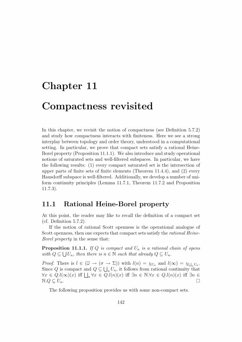
Chapter 11

Compactness revisited

In this chapter, we revisit the notion of compactness (see Definition 5.7.2)and study how compactness interacts with finiteness. Here we see a stronginterplay between topology and order theory, understood in a computationalsetting. In particular, we prove that compact sets satisfy a rational Heine-Borel property (Proposition 11.1.1). We also introduce and study operationalnotions of saturated sets and well-filtered subspaces. In particular, we havethe following results: (1) every compact saturated set is the intersection ofupper parts of finite sets of finite elements (Theorem 11.4.4), and (2) everyHausdorff subspace is well-filtered. Additionally, we develop a number of uni-form continuity principles (Lemma 11.7.1, Theorem 11.7.2 and Proposition11.7.3).

11.1 Rational Heine-Borel property

At this point, the reader may like to recall the definition of a compact set(cf. Definition 5.7.2).

If the notion of rational Scott openness is the operational analogue ofScott openness, then one expects that compact sets satisfy the rational Heine-Borel property in the sense that:

Proposition 11.1.1. If Q is compact and Un is a rational chain of openswith Q ⊆

⋃Un, then there is n ∈ N such that already Q ⊆ Un.

Proof. There is l ∈ (ω → (σ → Σ)) with l(n) = χUn and l(∞) = χSn Un .

Since Q is compact and Q ⊆⋃

n Un, it follows from rational continuity that∀x ∈ Q.l(∞)(x) iff

⊔n ∀x ∈ Q.l(n)(x) iff ∃n ∈ N.∀x ∈ Q.l(n)(x) iff ∃n ∈

N.Q ⊆ Un.

The following proposition provides us with some non-compact sets.

142

Proposition 11.1.2. The total elements of Nat and Baire do not formcompact sets.

Proof. Consider the program g ∈ (ω × Nat→ Σ) defined recursively by

g(x, n) = if x > 0 then (if n?= 0 then > else g(x− 1, pred(n))).

Clearly g(x, n) = > iff x > n for all x ∈ ω and n ∈ N. If the total elementsof N did form a compact set, then we would have u ∈ (ω → Σ) definedby u(x) = ∀n ∈ N.g(x, n) that would satisfy u(k) = ⊥ for all k ∈ N andu(∞) = > and hence would violate rational continuity. Therefore N is notcompact in Nat. If the total elements of Baire formed a compact set, then,considering f ∈ (Baire → Nat) defined by f(s) = s(0), the image of Bunder f is the set N which by Proposition 5.8.1(1) renders N compact, againproducing a contradiction.

Remark 11.1.3. The above proof relies on a continuity principle rather thanon recursion theory. Thus, compactness of N in Nat fails even if the languageincludes an oracle for the Halting Problem.

11.2 Saturation

Definition 11.2.1. The saturation of a subset S of a type σ is defined to bethe intersection of its open neighbourhoods and is denoted by sat(S), i.e.,

sat(S) =⋂U open |S ⊆ U.

A set S is said to be saturated if S = sat(S).

Lemma 11.2.2. Let S be a subset of a type.

(1) For any open set U , S ⊆ U iff sat(S) ⊆ U .

(2) ↑ S ⊆ sat(S).

(3) sat(S) is saturated.

(4) sat(S) is the largest set with the same neighbourhoods as S.

Proof. Clearly S ⊆ sat(S). Hence sat(S) ⊆ U implies S ⊆ U . Conversely,if S ⊆ U , then by construction of sat(S), sat(S) ⊆ U . Hence (1) holds. Ift ∈↑ S, then s v t for some s ∈ S. Hence t belongs to every neighbourhoodof S, and hence to sat(S). Therefore ↑ S ⊆ sat(S), i.e. (2) holds. Since

143

S ⊆ sat(S) for all S, we have that sat(S) ⊆ sat(sat(S)). Now supposex ∈ sat(sat(S)). Then for each open U with S ⊆ U , it holds that sat(S) ⊆ U .Thus x ∈ sat(S) by definition. Hence sat(S) = sat(sat(S)), i.e., (3) holds.That (4) holds is clear.

Remark 11.2.3. The inclusion in (2) is strict in general. Here we fur-nish with an example of S for which the set-inclusion is strict. Take S =(⊥,>), (>,⊥) of type Σ×Σ in a sequential language. Because of sequen-tiality, sat(S) =↑ (⊥,⊥). Then (⊥,⊥) ∈ sat(S) but (⊥,⊥) /∈↑ S.

Corollary 11.2.4. (1) Q is compact iff sat(Q) is compact, and in thiscase, ∀Q = ∀sat(Q).

(2) For any compact sets Q and R of the same type, it holds that ∀Q v ∀R

iff R ⊆ sat(Q).

Proof. (1) This is immediate in the light of Lemma 11.2.2(1).(2)

∀Q v ∀R

⇐⇒ ∀U ∈ U .∀Q(χU) = > ⇒ ∀R(χU) = >⇐⇒ ∀U ∈ U .Q ⊆ U ⇒ R ⊆ U⇐⇒ R ⊆

⋂U ∈ U|Q ⊆ U

⇐⇒ R ⊆ sat(Q)

Definition 11.2.5. Let X be a subspace of σ and S ⊆ X. The saturationof S with respect to the subspace X (X-saturation of S, for short) is definedto be the intersection of its relatively open neighbourhoods and is denotedby satX(S), i.e.,

satX(S) =⋂V open in X|S ⊆ V .

S is said to be X-saturated if S = satX(S).

Proposition 11.2.6. Let S ⊆ X ⊆ σ. Then satX(S) = X ∩ satσ(S). Hencefor every saturated subset S of σ, S ∩X is X-saturated.

Proof.

satX(S) =⋂V open in X|S ⊆ V

=⋂U ∩X|S ⊆ U ∩X ∧ U open in σ

= X ∩⋂U open in X|S ⊆ U

= X ∩ satσ(S)

144

The following is an extension of Corollary 11.2.4.

Proposition 11.2.7. Let Q, R ⊆ X ⊆ σ be compact sets. Then ∀Q v ∀R iffsatX(R) ⊆ satX(Q). So, if Q and R are X-saturated then

∀Q v ∀R ⇐⇒ R ⊆ Q.

Proof. Using Corollary 11.2.4 and Proposition 11.2.6, we have

∀Q v ∀R ⇐⇒ R ⊆ sat(Q)

⇐⇒ R ⊆ X ∩ sat(Q)

⇐⇒ R ⊆ satX(Q)

⇐⇒ satX(R) ⊆ satX(Q).

11.3 Compact open sets

The following is a characterisation of compact open sets:

Proposition 11.3.1. An open set is compact iff it has finite characteristic.Hence every open set is a rational union of compact open sets.

Proof. By Proposition 5.7.1(1), an open set V is compact iff the collectionU open |V ⊆ U is open iff χU |U open and V ⊆ U is open iff ↑ χV

is open. It then follows from Theorem 10.3.14 that this is equivalent toχV being finite, i.e., V having finite characteristic. The last part of theproposition then follows from Lemma 10.3.13(4).

11.4 Compact saturated sets

Armed with the results we have so far, it is easy to see that:

Proposition 11.4.1. Let U be an open set. If U = U (n), then U =↑ idn(U).Hence every open set of finite characteristic is the contextual upper set of afinite set of finite elements.

Proof. For each u ∈ U , it holds that idn(u) v u. Thus U ⊆↑ idn(U). Forthe reverse inclusion, pick x ∈↑ idn(U). Then there is u ∈ U such thatidn(u) v x. Because U = id−1

n (U) we have u ∈ id−1n (U). So idn(u) ∈ U and

hence x ∈ U .

145

The following may be seen as a generalisation of Theorem 10.3.14.

Proposition 11.4.2. If F is a finite set of finite elements, then sat(F ) isan open of finite characteristic.

Proof. For each x ∈ F , there exists nx such that idnx(x) = x. Let n =maxnx|x ∈ F. Then idn(x) = x for all x ∈ F . Hence if F ⊆ U for someopen U , then F ⊆ id−1

n (U) ⊆ U . So sat(F ) =⋂id−1

n (U)|F ⊆ U. Becausethis is the intersection of a finite set of open sets, it is open. Moreover, bythe idempotence of idn, we have:

(sat(F ))(n) = (⋂U (n)|F ⊆ U,U open)(n)

=⋂(U (n))(n)|F ⊆ U,U open

=⋂U (n)|F ⊆ U,U open

= sat(F ).

Lemma 11.4.3. If Q is compact, then idn(Q) is compact and

idn(∀Q) = ∀idn(Q).

Furthermore, if U is open with Q ⊆ U , then there is n such that idn(Q) ⊆ U .

Proof. That idn(Q) is compact and idn(Q) = ∀idn(Q) follow immediately fromProposition 5.8(1). Now, if U is open with Q ⊆ U , then ∀Q(χU) = >. Henceby rational continuity there is n such that already idn(∀Q)(χU) = >, i.e.,∀idn(Q)(χU) = >. So there is n such that idn(Q) ⊆ U .

Theorem 11.4.4. If Q is compact then sat(Q) =⋂

n sat(idn(Q)). Henceevery compact saturated set is the intersection of upper parts of finite sets offinite elements.

Proof. Since for any n it holds that idn(Q) ⊆ U implies Q ⊆ U , it follows thatQ ⊆ sat(idn(Q)). Thus sat(Q) ⊆

⋂n sat(idn(Q)). For the reverse inclusion,

take any U open with Q ⊆ U . Then there is n such that idn(Q) ⊆ U andhence sat(idn(Q)) ⊆ U . Hence sat(Q) =

⋂n sat(idn(Q)).

11.5 Intersections of compact saturated sets

A family of compact sets Qii is said to be rationally filtered if (∀Qi)i is a

rational chain in (σ → Σ) → Σ.

146

Proposition 11.5.1. Let X be a subspace of σ and Qii a rationally filteredfamily of compact X-saturated subsets of X. Then the following statementsare equivalent:

(i)⋂

i Qi is compact and ∀Ti Qi

v⊔

i ∀Qi.

(ii)⊔

i ∀Qiuniversally quantifies over

⋂i Qi.

(iii) For every open set U in σ,⋂i

Qi ⊆ U =⇒ ∃i.Qi ⊆ U.

Proof. Observe that (a) if⋂

i Qi is compact, then by Corollary 11.2.4 theinequality ∀T

i Qiw

⊔i ∀Qi

always holds, and (b) the inequality in (i) is equiv-alent to the implication in (iii).(i) ⇐⇒ (ii): This is immediate from observation (a).(i) =⇒ (iii): This follows from observation (b).(iii) =⇒ (ii): It suffices to show that for every open set U in σ, it holds that⊔

i

∀Qi(χU) = > ⇐⇒

⋂i

Qi ⊆ U.

(=⇒):⊔

i ∀Qi(χU) = > implies the existence of i such that ∀Qi

(χU) = >.Thus Qi ⊆ U and since

⋂i Qi ⊆ Qi, it follows that

⋂i Qi ⊆ U .

(⇐=): Suppose that⋂

i Qi ⊆ U . By assumption, there is i such that Qi ⊆ U .So ∀Qi

(χU) = > and hence⊔

i ∀Qi(χU) = >.

11.6 A non-trivial example of a compact set

The simplest non-trivial example of a compact set, which is a manifestationof the “one-point compactification of the discrete space of natural numbers”,is given in the following proposition.

We regard function types of the form (Nat → σ) as sequence types anddefine “head”, “tail” and “cons” constructs for sequences as follows:

(1) hd(s) = s(0) and tl(s) = λi.s(i + 1).

(2) n :: s = λi.if i?= 0 then n else s(i− 1).

We also use familiar notations such as 0n1ω as shorthands for evident termssuch as λi.if i < n then 0 else 1.

147

Proposition 11.6.1. The set N∞ of sequences of the forms 0n1ω and 0ω iscompact in Baire.

Proof. Define, omitting the subscript N∞ for ∀,

∀(p) = p(if (p(1ω) ∧ ∀(λs.p(0 :: s))) then t)

where t is some element of N∞. More formally, ∀ = fix(F ) where

F (A)(p) = p(if (p(1ω) ∧ A(λs.p(0 :: s))) then t).

We must show that, for any given p, ∀(p) = > iff p(s) = > for all s ∈ N∞.(⇐=): The hypothesis gives p(0ω) = >. By Proposition 10.2.6, there isn ∈ N such that already p(idn(0ω)) = >. Recall that

idn(0ω)(i) =

0 if i < n;

⊥ otherwise.

We now show by induction on k that:

For all p ∈ (Baire→ Σ) such that p(s) = > for every s ∈ N∞,

p(idk(0ω)) = > =⇒ F k(⊥)(p) = >.

Base case: k = 0This means that p is the constant predicate λs.> and the hypothesis holdstrivially.Inductive step:Suppose that p ∈ (Baire → Σ) such that p(s) = > for all s ∈ N∞ and thatp(idk+1(0

ω)) = >. Unwinding the definition of F reveals that

F k+1(⊥)(p) = F (F k(⊥))(p)= p(if (p(1ω) ∧ F k(⊥)(λs.p(0 :: s))) then t) (by definition of F )= p(if (F k(⊥)(λs.p(0 :: s))) then t) (since p(1ω) = >)

Denote the predicate λs.p(0 :: s) by q. Because (0 :: s) ∈ N∞ whenevers ∈ N∞, it holds that q(s) = > for every s ∈ N∞. Moreover p(idk+1(0

ω)) = >implies that q(idk(0

ω)) = >. Hence by the induction hypothesis we have thatF k(⊥)(q) = >. Thus F k+1(⊥)(p) = p(t) = > as desired.

Because F n(⊥) v ∀, it follows that ∀(p) = >.

(=⇒): By rational continuity, the hypothesis implies that F n(⊥)(p) = > forsome n. We now prove by induction on k that:

148

For all q ∈ (Baire→ Σ), F k(⊥)(q) = ⊥ =⇒ q(s) = > for all s ∈ N∞.

Base case: k = 0This is vacuously true.Inductive step:Suppose F k+1(⊥)(q) = >. But unfolding F k+1(⊥) gives

F k+1(⊥)(q) = q(if (q(1ω) ∧ F k(⊥)(λs.q(0 :: s))) then t.

So it must be that q(1ω) = > and F k(⊥)(λs.q(0 :: s)) = >. It then followsfrom the induction hypothesis that q(0 :: s) = > for all s ∈ N∞. But sinceevery t ∈ N∞ is either of the form 1ω or 0 :: s for some s ∈ N∞, the resultfollows.

11.7 Uniform-continuity principles

In this section, we consider some uniform continuity principles.

Lemma 11.7.1. For total f ∈ (σ → Baire) and Q a compact set of totalelements of σ,

∀ε ∈ N.∃δ ∈ N.∀x ∈ Q.f(x) ≡ε f(idδ(x))

where x ≡n x′ denotes idn(x) = idn(x′).

Proof. For any given ε, we construct the following program e ∈ (Baire ×Baire→ Σ).

E : Baire× Baire× Nat→ ΣE(s, t, n) = if n

?= 0 then > else (if s(n) = t(n) then E(s, t, pred(n)))

e(s, t) = E(s, t, ε).Then this program e is such that

(1) if s, t ∈ Baire are total then s ≡ε t =⇒ e(s, t) = >,

(2) for all s, t ∈ Baire, e(s, t) = > =⇒ s ≡ε t.

Note that both (1) and (2) can be easily proven by induction on ε.If we define p(x) := e(f(x), f(x)), then, by hypothesis and (1), ∀Q(p) = >.

By Proposition 10.2.6, ∀Q(idδ(x)) = > for some δ ∈ N, and, by Proposition10.3.9(2), idδ(p)(x) = p(idδ(x)). It follows that e(f(idδ(x)), f(idδ(x))) = >for all x ∈ Q. By monotonicity, e(f(x), f(idδ(x))) = >, and, by (2), f(x) ≡ε

f(idδ(x)), as required.

149

Theorem 11.7.2. For f ∈ (σ → Baire) total and Q a compact set of totalelements of σ,

∀ε ∈ N.∃δ ∈ N.∀x, y ∈ Q.x =δ y =⇒ f(x) =ε f(y).

Proof. Given ε ∈ N, first construct δ ∈ N as in Lemma 11.7.1. For x, y ∈ Q,if x =δ y then idε(f(x)) = idε(f(idδ(x))) = idε(f(idδ(y))) v f(y). By Lemma10.4.7, idε(f(x)) = idε(f(y)), as required.

Similarly, we have:

Proposition 11.7.3. For γ ∈ Nat, Bool, Σ, f ∈ (σ → γ) total and Q acompact set of total elements of σ,

(1) ∃δ ∈ N.∀x ∈ Q.f(x) = f(idδ(x)),

(2) ∃δ ∈ N.∀x, y ∈ Q.x =δ y =⇒ f(x) = f(y).

Proof. (1) Recall that there is an equality test (==) ∈ (γ × γ → Σ) forthe total elements of γ such that

(a) if x, y ∈ γ are total then x = y =⇒ (x == y) = >,

(b) for all x, y ∈ γ, (x == y) = > =⇒ x = y.

If we define p(x) := (f(x) == f(x)) then ∀Q(x) = > by hypothe-sis and (a). By Proposition 10.2.6, ∀Q(idδ(p)) = > for some δ ∈ N.Since idδ(p)(x) = p(idδ(x)) by Proposition 10.3.9(2), it follows that(f(idδ(x)) == f(idδ(x))) = > for all x ∈ Q and, by monotonicity,(f(x) == f(idδ(x))) = >, and, by (b), f(x) = f(idδ(x)), as required.

(2) From (1) there exists δ ∈ N such that for all x ∈ Q, f(x) = f(idδ(x)).Thus for all x, y ∈ Q, if x =δ y then f(x) = f(idδ(x)) = f(idδ(y)) =f(y).

Definition 11.7.4. For f and Q as in Proposition 11.7.3, we refer to theleast δ ∈ N such that (1) (respectively (2)) holds as the big (respectivelysmall) modulus of uniform continuity of f at Q. From the above proof, itis clear that the small modulus is smaller than or equal to the big modulus.

150

Chapter 12

Sample applications

In this chapter, we illustrate the scope and flexibility of the operationaldomain theory developed so far by applying our conclusions in the previouschapters to prove the correctness of non-trivial programs that manipulateinfinite data (see Section 12.3 - 12.5).

We use the data language D to formulate specifications of programs inthe programming language P . The notion of data language originates fromEscardo [13]. For the purpose of this chapter, P and D do not includeparallel features. As in Section 3.7, the notation x ∈ σ means that x is aclosed term of type σ in D. This is compatible with the notation of Chapters9 - 11 by taking D as the underlying language for them. Again maintainingcompatibility, we take the notions of totality, open set and compact set withrespect to D. To indicate that openness or compactness of a set is witnessedby a program rather than just an element of the data language, we sayprogrammably open or compact.

Like the Baire type, we think of the elements of the Cantor type assequences, and, following topological tradition, in this context we identifythe booleans true and false with numbers 0 and 1 (it does not matter inwhich order).

12.1 Data language: an extension with ora-

cles

In an operational setting, one usually adopts the same language to constructprograms of a type and to express data of the same type. But considerprograms that can accept externally produced streams as inputs. Becausesuch streams are not necessarily definable in the language, it makes senseto consider program equivalence define by quantification over more liberal

151

“data contexts” and ask whether the same notion of program equivalence isobtained.

Definition 12.1.1. Let P be the programming language PCF introducedin Chapter 3, perhaps extended with parallel features, but not with oracles,and let D be P extended with oracles. We think of D as a data languagefor the programming language P . The idea is that the closed term of Pare programs and those of D are (higher typed) data. Accordingly, in thiscontext, the notation x ∈ σ means that x is a closed term of type σ in thedata language. Of course, this includes the possibility that x is a program.

12.2 Equivalence with respect to ground D-

contexts

The following is folklore and goes back to Milner [38].

Theorem 12.2.1. For terms in P, equivalence with respect to ground P-contexts and equivalence with respect to ground D-contexts coincide.

Proof. This follows directly from Proposition 10.2.4 and Lemma 12.2.2 below.

Lemma 12.2.2. For any data element x of any type, idn(x) is equivalent tosome program with respect to ground D-context.

Proof. Given x ∈ σ in D, there exists a program g ∈ Bairem → σ and oraclesΩ1, . . . , Ωm such that x = g(Ω1, . . . , Ωm). It follows from m applications ofProposition 10.4.2 that there exist k1, . . . , km such that

idn(x) = idn(g(idk1(Ω1), . . . , idkm(Ωm))).

But the right-hand term is equivalent to a program, because clearly for anyoracle Ω and n ∈ N, the data term idn(Ω) is equivalent to some program.

On the other hand, the notion of totality changes:

Theorem 12.2.3. There are programs that are total with respect to P butnot with respect to D.

This kind of phenomenon is again folklore. There are programs of type,for instance Cantor → Bool, where Cantor := (Nat → Bool), that, whenseen from the point of view of the data language, map programmable to-tal elements to total elements, but diverge at some non-programmable total

152

inputs. The construction uses Kleene trees (see Beeson [4]), which are recur-sive counter-examples to Konig’s Lemma, and can be found in Section 3.11of Escardo [13].

12.3 The Cantor space

In this section, we are ready to give a more sophisticated example of a com-pact space. The following also serves as our main tool in this chapter:

Theorem 12.3.1. (Escardo [13], Section 3.11) The total elements of theCantor type, C, form a programmably compact set.

Proof. The universal quantification program ∀ : (Cantor → Σ) → Σ can bedefined recursively by:

∀(p) = p(if ∀(λs.p(0 :: s)) ∧ ∀(λs.p(1 :: s)) then t)

where t is some programmable total element of Cantor, such as 0ω. Formally,∀ = fix(F ) where

F (A)(p) = p(if A(λs.p(0 :: s)) ∧ A(λs.p(1 :: s)) then t)

It remains to prove the correctness of this program, i.e.,

∀(p) = > iff ∀s ∈ C.p(s) = >.

(=⇒): By rational continuity, the hypothesis implies that already F n(⊥)(p) => for some n ∈ N. We now prove by induction on k that:

∀q.F k(⊥)(q) = > ⇒ q(s) for all s ∈ C.

Base case: k = 0Because q does not look at its argument and returns >, it must be theconstant predicate λs.>. Thus q(s) = > for all s ∈ C in particular.Inductive step:Suppose F k+1(⊥)(q) = >. Unfolding F yields:

F (F k(⊥))(q) = q(if (F k(⊥)(λs.q(0 :: s)) ∧ F k(⊥)(λs.q(1 :: s))) then t)

Thus it must be that F k(⊥)(λs.q(0 :: s)) = > = F k(⊥)(λs.q(1 :: s)). In-voking the induction hypothesis, we deduce that both (λs.q(0 :: s)) and(λs.q(1 :: s)) hold for all s ∈ C. Because every element of C has to beginwith either 0 or 1, it follows that q holds for all s ∈ C.

153

(⇐=): The hypothesis gives p(s) = > for all s ∈ C. Notice that for each suchgiven s ∈ C, there is n ∈ N such that already p(idn(s)) = >. By the Cantortree we mean the infinite binarily branching tree. We think of an elementof C as an infinite path in the Cantor tree, starting from the root, where asequence of digits 0 and 1 is interpreted as a sequence of instructions “turnleft” and “turn right”. Since p looks only at the first n positions of the paths, it induces a pruning of s at level n; after which p does not look at the restof the path. Because p(s) = > for every path s in the Cantor tree, we pruneall possible paths and this results in a finitely branching tree of which everypath is finite. By Konig’s Lemma, the resulting pruned tree is finite, i.e., theheight of the tree is finite, which we denote by δ. Thus it is clear that for alls ∈ C, p(s) = p(idδ(s)) = >. This is precisely the big modulus of uniformcontinuity of p at C (cf. Definition 11.7.4).

Now we prove by induction on δ that:

If the big modulus of uniform continuity of p at C is δ, then ∀(p) = >.

Base case: δ = 0p does not look at its argument and returns >. From the way ∀ is defined,it holds that ∀(p) = >.Inductive step:Suppose the big modulus of uniform continuity of p at C is δ + 1. Unfolding∀(p) yields:

p(if (∀(p0) ∧ ∀(p1)) then t)

where p0 := λs.p(0 :: s) and p1 := λs.p(1 :: s). Notice that the big moduliof continuity of these predicates p0 and p1 at C are at most δ. Invoking theinduction hypothesis on p0 and p1, it follows that ∀(p0) = > = ∀(p1). It thenfollows, from the hypothesis and t ∈ C, that ∀(p) = >, as required.

Remark 12.3.2. If the data language is taken to be P itself, Theorem12.3.1 fails for the same reason that leads to Theorem 12.2.3. Of course,the above program can still be written down. But it no longer satisfies therequired specification given in Proposition 5.7.1(2). In summary, it is easierto universally quantify over all total elements of the Cantor type than justover the programmable ones, to the extent that the former can be achievedby a program but the latter cannot.

Interestingly, the programmability conclusion of Theorem 12.3.1 is notinvoked for the purposes of this chapter, because we only apply compactnessto get uniform continuity.

154

12.4 Universal quantification for boolean-valued

predicates

The following theorem is due to Berger [5], with domain-theoretic denota-tional specification and proof. As discussed in the introduction, our purposeis to illustrate that such specifications and proofs can be directly understoodin our operational setting, and, moreover, apply to sequential programminglanguages.

Theorem 12.4.1. There is a total program

ε : (Cantor→ Bool) → Cantor

such that for any total p ∈ (Cantor → Bool), if p(s) = 0 for some totals ∈ Cantor, then ε(p) is such an s.

Proof. Define

ε(p) = if p(0 :: ε(λs.p(0 :: s)) then 0 :: ε(λs.p(0 :: s))else 1 :: ε(λs.p(1 :: s))

Since C is compact, every total (boolean-valued) predicate p has a big mod-ulus of uniform continuity δ. We now prove by induction on δ that:If the big modulus of uniform continuity of p at C is δ, then p(s) = 0 forsome total s ∈ Cantor implies that ε(p) is such an s.Base case: δ = 0When p has a modulus zero, p(⊥) is total and hence p is constant. So irre-spective of what ε(p) is, we always have p(ε(p)) = 0.Inductive step:If p has modulus δ + 1, then the predicates p0 := λs.p(0 :: s) and p1 :=λs.p(1 :: s) have modulus at most δ. Given that p(s) = 0 for some s ∈ C.Without loss of generality, let us assume that s is of the form 0 :: t for somet ∈ C. Thus we have p0(t) = 0 and it follows from the induction hypothesisthat ε(p0) witnesses p0, i.e., p0(ε(p0))) = 0. By the definition of ε, we haveε(p) = 0 :: ε(p0). Now p(ε(p)) = p(0 :: ε(p0)) = p0(ε(p0)) = 0. Thus ε(p) is atotal element from Cantor that witnesses p.

This gives rise to universal quantification for boolean-valued rather thanSierpinski-valued predicates:

Corollary 12.4.2. There is a total program

∀′ : (Cantor→ Bool) → Bool

155

such that for every total p ∈ (Cantor→ Bool),

∀′(p) = 0 iff p(s) = 0 for all total s ∈ Cantor.

Proof. First define ∃ : (Cantor→ Bool) → Bool by ∃(p) = p(ε(p)) and thendefine ∀′(p) = ¬(∃(λs.¬p(s))). If p(s) for some total s ∈ Cantor, then byTheorem 12.4.1 it holds that ε(s) is a witness to p, i.e., ∃(p) = p(ε(p)) = 0.Conversely if ∃(p) = 0 then p(ε(p)) = 0. This means p(s) = 0 for some totals ∈ Cantor (in which case, s = ε(p)). Thus in summary we have:

∃(p) = 0 iff p(s) = 0 for some total s ∈ Cantor.

Unwinding the definition of ∀′, we see that ∀′(p) = 0 iff ∃(λs.¬p(s)) = 1 iff¬p(s) = 1 for all total s ∈ Cantor iff p(s) = 0 for all total s ∈ Cantor.

So quite surprising one has:

Corollary 12.4.3. The function type (Cantor→ Nat) has decidable equalityfor total elements.

Proof. Define a program

(==) : (Cantor→ Nat)× (Cantor→ Nat) → Bool

by f == g := ∀′(λs.f(s) == g(s)) where the second == is the equalitytest on the total elements of Nat. It is easy to see that (f == g) = 0 ifff(s) == g(s) for all total s ∈ Cantor.

12.5 The supremum of the values of a func-

tion

The lexicographic order on the total elements of the Baire type is defined bys ≤ t iff whenever s 6= t, there is n ∈ N with s(n) < t(n) and s(i) = t(i) forall i < n.

Lemma 12.5.1. There is a total program

max : Baire× Baire→ Baire

such that

156

1. max(s, t) is the maximum of s and t in the lexicographic order of alltotal s, t ∈ Baire, and

2. (s, t) ≡ε (s′, t′) ⇒ max(s, t) ≡ε max(s′, t′) for all s, t, s′, t′ ∈ Baire

(total or not) and all ε ∈ N.

Proof. Define the program

max(s, t) = if hd(s) == hd(t)then hd(s) :: max(tl(s), tl(t))else (if (hd(s) > hd(t) then s else t).

1. We now show that for all total s, t ∈ Baire,

max(s, t) = t ⇐⇒ s ≤ t.

Case 1: s 6= t.For a given pair s 6= t we define the minimum n ∈ N for which s(n) 6=t(n) as the disagreement index of s and t. We prove by induction on nthat:For every total s, t ∈ Baire (s 6= t) whose disagreement index is n,

max(s, t) = t ⇐⇒ s ≤ t.

Base case: n = 0max(s, t) = t iff hd(s) < hd(t) iff s(0) < t(0).Inductive step:Suppose s 6= t ∈ Baire with disagreement index of n + 1. Thenmax(s, t) = hd(s) :: max(tl(s), tl(t)). Since tl(s) 6= tl(t) has disagree-ment index n, it follows from the induction hypothesis that

max(tl(s), tl(t)) = tl(t) ⇐⇒ tl(s) ≤ tl(t).

It immediately follows that max(s, t) = t ⇐⇒ ≤ t.

Case 2: s = t.We prove by induction on k that for all k ∈ N, for all total s ∈ Baire,it holds that

max(s, s)(k) = s(k)

which then implies that max(s, s) = s by extensionality.Base case: k = 0Since hd(s) == hd(s), we have max(s, s) = hd(s) :: max(tl(s), tl(s)).

157

Hence max(s, s)(0) = hd(max(s, s)) = hd(s) = s(0).Inductive step:

max(s, s)(k + 1) = (hd(s) :: max(tl(s), tl(s)))(k + 1)= max(tl(s), tl(s))(k)= tl(s)(k)= s(k + 1).

2. By induction on ε.

The following is an adaptation of an example taken from Simpson [52].In order to avoid having exact real-number computation as a pre-requisite,as in this reference, we have made suitable modifications to the program andits specification but retaining their essential aspects.

Theorem 12.5.2. There is a total program

S : (Cantor→ Baire) → Baire

such that for every total f ∈ (Cantor→ Baire),

S(f) = supf(s)|s ∈ Cantor is total,

where the supremum is taken in the lexicographic order.

Proof. Let t ∈ Cantor be a programmable total element and define

S(f) = if ∀′(λs.hd(f(s)) == hd(f(t)))

then hd(f(t)) :: S(λs.tl(f(s)))

else max(S(λs.f(0 :: s)), S(λs.f(1 :: s)))

where ∀′ : (Cantor→ Bool) → Bool is the total program in Corollary 12.4.2.For convenience, we use the following notation:

supf(s)|s ∈ Cantor is total := sup f.

We show by induction on n ∈ N that, for every total f ∈ (Cantor→ Baire),

S(f) ≡n sup f.

Recall that x ≡n y ⇐⇒ idn(x) = idn(y).Base case: n = 0.

158

Trivial.Inductive step:Assume that the statement holds for n, we must show that for every totalf ∈ (Cantor→ Baire), it holds that

S(f) ≡n+1 sup f.

Recall from Proposition 11.7.4(2) that for each total f ∈ (Cantor→ Baire),the total function hd f ∈ (Cantor→ Nat) has a small modulus of uniformcontinuity , denoted by δ. We now prove by a further induction on δ that,for every total f ∈ (Cantor→ Baire) such that hd f has modulus δ,

S(f) ≡n+1 sup f.

Base case: δ = 0.If hd f has modulus 0 then hd f is a constant, i.e. hd(f(s)) = hd(f(t))for all total s. So S(f) = hd(f(t)) :: S(λs.tl(f(s))). But by assumption,S(λs.tl(f(s))) ≡n sup(λs.tl(f(s))), and thus:

S(f) = hd(f(t)) :: S(λs.tl(f(s)))≡n+1 hd(f(t)) :: sup (λs.tl(f(s)))= sup((λs.hd(f(t)) :: s) (λs.tl(f(s))))= sup f.

Note that the second equality relies on the fact that for all h,

sup((λs.d :: s) h) = d :: sup h.

Inductive step:If hd f has modulus δ + 1 then hd (λs.f(0 :: s)) and hd (λs.f(1 :: s))have modulus δ. Then hd f(s) 6= hd f(t) for some total s ∈ Cantor.Thus S(f) = max(S(λs.f(0 :: s)), S(λs.f(1 :: s))). By assumption, we haveS(λs.f(0 :: s)) ≡n sup(λs.f(0 :: s)) and S(λs.f(1 :: s)) ≡n sup(λs.f(1 :: s)).And by the (second) induction hypothesis, we have S(λs.f(0 :: s)) ≡n+1

sup(λs.f(0 :: s)) and S(λs.f(1 :: s)) ≡n+1 sup(λs.f(1 :: s)). Now by the non-expansiveness property given by Lemma 12.5.1(2) we have that S(f) ≡n+1

max(sup(λs.f(0 :: s)), sup(λs.f(1 :: s))). Finally, we use the fact that

sup h = max(sup(λs.h(0 :: s)), sup(λs.h(1 :: s)))

to deduce that max(sup(λs.f(0 :: s)), sup(λs.f(1 :: s))) = sup f . HenceS(f) ≡n+1 sup f and this completes the second induction.

159

Thus by Lemma 10.4.7, S(f) =n sup f for all n ∈ N, and by Lemma 10.3.2it follows that

S(f) = sup f.

160

Part IV

Operational Domain Theory forFPC

161

In this part, an operational domain theory is developed for FPC to treatrecursive types. In Chapter 13, we establish the functoriality of type ex-pressions. In Chapter 14, we establish the operational algebraic compactnessof both the diagonal category, FPC!

δ, and the product category, ˘FPC!.In Chapter 15, we derive a pre-deflationary structure on the closed typesand develop, as a consequence of this, a proof technique called the GenericApproximation Lemma. We demonstrate the versatility of this lemma in es-tablishing program equivalence, where previously many other more complexmethods had been employed.

162

Chapter 13

FPC considered as a category

The purpose of this chapter is to set up an appropriate categorical frameworkupon which an operational domain-theoretic treatment of recursive types canbe carried out. In this chapter, we show how FPC types-in-context can beviewed as realisable functors. In order to achieve this, we prove operationalversions of the Plotkin’s uniformity principle (also known as the Plotkin’saxiom) and the minimal invariance property.

The first category we consider, called FPC!, allows us to interpret types-in-context X1, . . . , Xn ` σ as functors FPCn

! → FPC!, provided type recur-sion in σ does not occur in contravariant positions (Sections 13.1 and 13.2).The second category, which is constructed out of FPC!, called FPC!

δ, allowsus to remove this restriction (Section 13.3).

13.1 The category of FPC types

The main purpose of this chapter is to give an account of the categoricalframework within which our theory is organised. Our approach, largelyadapted from Abadi & Fiore [1], turns out to be a convenient option amongothers. We carefully explain this in two stages:

(i) understand the basic type expressions (i.e., type expressions in whichtype recursion does not occur in contravariant positions) as functors,and then

(ii) consider those built from all possible type constructors.

The objects of the category FPC are the closed FPC types (i.e., typeexpressions with no free variables) and the morphisms are closed terms offunction-type (modulo contextual equivalence). Given closed type σ, the

163

identity morphism idσ is just the closed term λxσ.x and the composition oftwo morphisms f and g is defined as

g f := λx.g(f(x)).

The category FPC! is the subcategory of FPC whose morphisms are thestrict FPC-morphisms.

We make use of the following notations:

~σ for a sequence of closed types σ1, . . . , σn;~t for a sequence of closed terms t1, . . . , tn;~X for a sequence of type variables X1, . . . , Xn;~x for a sequence of term variables x1, . . . , xn;

~σ/ ~X for the substitutions σ1/X1, . . . , σn/Xn;~t/~x for the substitutions t1/x1, . . . , tn/xn;~f : ~R → ~S for f1 : R1 → S1, . . . , fn : Rn → Sn.

When we write ~X, X, it is understood that X does not appear in ~X.

13.2 Basic functors

FPC type expressions are called basic if they are generated by the followingfragment of the grammar:

B := C |X | B× B | B + B | B⊥ | µX.B| C→ B

where C ranges over closed types. Note that the set of basic type expressionsis a proper subset of those type expressions in which recursion does not occurin the contravariant positions. For instance, µX.((X → C) → C is not basic.

A basic functor T : FPCn! → FPC! is one realised by:

(1) a basic type-in-context ~X ` τ ;

(2) a term-in-context

~R, ~S; ~f : ~R → ~S ` t : τ [~R/ ~X] → τ [~S/ ~X]

such that for any ~σ ∈ FPCn! , it holds that

T (~σ) = τ [~σ/ ~X]

164

and for any ~ρ and ~σ, and any ~v ∈ FPC!(~ρ, ~σ), it holds that

T (~v) = t[~v/~f ].

Now we show how basic type expressions define basic functors. We firstpresent the construction and then prove functoriality. For a basic type ex-pression B in context Θ ≡ ~X, we define, by induction on the structure oftypes, an associated functor SΘ`B : FPCn

! → FPC! (or simply S) as follows:

(1) Closed type.Let Θ ` C.For object ~σ ∈ FPCn

! , define S(~σ) = C.For morphism ~v ∈ FPC!(~ρ, ~σ), define S(~v) = idC.

(2) Type variable.Let Θ ` Xi (i ∈ 1, . . . , n).For object ~σ ∈ FPCn

! , define S(~σ) = σi.For morphism ~v ∈ FPC!(~ρ, ~σ), define S(~v) = vi.

Let Θ ` B1, B2 be given. Assume that Tj (j = 1, 2) is the basic functorassociated with Θ ` Bj, whose morphism part is realised by

~R, ~S; ~f : ~R → ~S ` tj : Bj[~R/ ~X] → Bj[~S/ ~X].

(3) Product type.For object ~σ ∈ FPCn

! , define S(~σ) = T1(~σ)× T2(~σ).For morphism ~v ∈ FPC!(~ρ, ~σ), define S(~v) to be the unique morphismh such that the following diagram

S(~ρ)πj - Tj(~ρ)

S(~σ)

h

?

πj

- Tj(~σ)

Tj(~v)

?

commutes (j = 1, 2). The morphism part of S is realised by

~R, ~S; ~f : ~R → ~S ` λz.(t1(π1z).t2(π2z)).

(4) Sum type.

165

For object ~σ ∈ FPCn! , define S(~σ) = T1(~σ) + T2(~σ).

For morphism ~v ∈ FPC!(~ρ, ~σ), define S(~v) to be the unique morphismh which makes the diagrams

S(~ρ) inl

T1(~ρ) S(~ρ) inr

T2(~ρ)

S(~σ)

h

?

inlT1(~σ)

T1(~v)

?

S(~σ)

h

?

inrT2(~σ)

T2(~v)

?

commute. The morphism part of S is realised by

~R; ~S; ~f : ~R → ~S ` λz.case(z)of

inl(x).inl(t1(x))

inr(y).inr(t2(y))

(5) Lifted type.Let Θ ` B be given and T its associated basic functor.For object ~σ ∈ FPCn

! , define S(~σ) = (T (~σ))⊥.For morphism ~v ∈ FPC!(~ρ, ~σ), define S(~v) to be the unique morphismh which makes the diagram

S(~ρ) up

T (~ρ)

S(~ρ)

h

?

upT (~σ)

T (~v)

?


~R, ~S; ~f : ~R → ~S ` λz.case(z) of up(x).up(t(x))

where the morphism part of T is realised by

~R, ~S; ~f : ~R → ~S ` t : B[~R/ ~X] → B[~S/ ~X].

(6) Recursive type.Let Θ, X ` B (X /∈ X1, . . . , Xn) and T the associated basic functor.

166

For object ~σ ∈ FPCn! , define S(~σ) = µX.T (~σ, X). We write T (~σ, S(~σ))

for B[~σ/ ~X, S(~σ)/X].For the morphism ~v ∈ FPC!(~ρ, ~σ), define S(~v) to be the least morphismh that makes the diagram

S(~ρ)unfoldS(~ρ)

- T (~ρ, S(~ρ))

S(~σ)

h

?

unfoldS(~σ)- T (~σ, S(~σ))

T (~v, h)

?


~R, ~S; ~f : ~R → ~S ` fix(λg.fold t[g/f ] unfold)


~R,R, ~S, S; ~f : ~R → ~S, f : R → S ` t : B[~R/ ~X, R/X] → B[~S/ ~X, S/X].

(7) Restricted function type.Let Θ ` B be given and T the associated functor. Let C be a closed type.We want to define the functor S which is associated to Θ ` C→ B.For object ~σ ∈ FPCn

! , define S(~σ) = C→ T (~σ).For morphism ~v ∈ FPC!(~ρ, ~σ), define S(~v) to be

λg : (C→ T (~ρ)) → (C→ T (~σ)).T (~v) g.

The morphism part of S is realised by

~R, ~S; ~f : ~R → ~S ` λg.t g


~R, ~S; ~f : ~R → ~S ` t : B[~R/ ~X] → B[~S/ ~X].

Functoriality relies on the following two key lemmas.

Lemma 13.2.1. (Plotkin’s uniformity principle)Let f : σ → σ, g : τ → τ be FPC programs and h : σ → τ be a strict program,

167

i.e., h(⊥σ) = ⊥τ , such that the following diagram

σh

- τ

σ

f

?

h- τ

g

?

commutes, i.e., g h = h f . Then it holds that

fix(g) = h(fix(f)).

Proof. Using rational-chain completeness, rational continuity, h f = g hin turn, it follows that

h(fix(f)) = h(⊔

n f (n)(⊥σ))=

⊔n h f (n)(⊥σ)

=⊔

n g(n) h(⊥σ)=

⊔n g(n)(⊥τ )

= fix(g).

Remark 13.2.2. Notice that this uniformity of least fixed point relies on therational-chain completeness enjoyed by FPC types and rational continuity offunction-type programs. Both facts have been established in Part II of thisthesis (cf. Theorem 7.6.6).

Lemma 13.2.3. (Operational minimal invariance for basic functors)Let T : FPCn+1

! → FPC! be a basic functor and ~σ any sequence of closedtypes. Write S(~σ) for µX.T (~σ, X). Then the least endomorphism e : S(~σ) →S(~σ) for which the diagram

S(~σ)unfoldS(~σ)

- T (~σ, S(~σ))

S(~σ)

e

?

unfoldS(~σ)- T (~σ, S(~σ))

T (~id, e)

?

168

commutes must be idS(~σ).

Proof. The interpretation of e in the Scott model, denoted by [[e]], makes thecorresponding diagram commute. By Theorem 2.3.7, the only such endomor-phism on [[S(~σ)]] must be id[[S(~σ)]]. Now, by Lemma 13.2.4 below, it followsthat e = idS(~σ).

Lemma 13.2.4. Let e : τ → τ be a closed term such that [[e]] = id[[τ ]] in theScott-model. Then e = idτ .

Proof. Notice that [[e]] = id[[τ ]] = [[idτ ]]. By Corollary 4.6.4, it follows thate = idτ .

We are now ready to prove functoriality. First we prove the preserva-tion of composition of morphisms. Consider the following composition ofmorphisms:

~σ~u

- ~ρ~v

- ~τ

It is easy to see that type expressions which are of the following forms: typevariables, sum types, product types and lifted types, preserve compositionas the corresponding constituent functors do. Thus, it remains to verify thatconstructors of the form µX.T ( ~X, X) do preserve the above composition,i.e., the following diagram commutes:

µX.T (~σ, X)µX.T (~u, X)

- µX.T (~ρ,X)µX.T (~v, X)

- µX.T (~τ , X)

µX.T (~σ, X)

=

?

µX.T (~v ~u, X)- µX.T (~τ , X)

=

6

Let us abbreviate µX.T (~σ, X) by S(~σ) as before.Consider the following diagram:

(S(~ρ) → S(~τ))− S(~u)

- (S(~σ) → S(~τ))

(S(~ρ) → S(~τ))

Φ

?

− S(~u)- (S(~σ) → S(~τ))

Ψ

?

169

where Φ = λh.foldS(~τ) T (~v, h) unfoldS(~ρ) andΨ = λf.foldS(~τ) T (~v ~u, f) unfoldS(~σ).

The diagram commutes because for any h : S(~ρ) → S(~τ),

Ψ(h S(~v))

= foldS(~τ) T (~v ~u, h S(~u)) unfoldS(~σ)

= foldS(~τ) T (~v, h) unfoldS(~ρ) foldS(~ρ) T (~u, S(~u)) unfoldS(~σ)

= Φ(h) S(~u)

Because − S(~u) is a strict program, by Lemma 13.2.1 it follows that

S(~v ~u) = fix(Ψ) = fix(Φ) S(~u) = S(~v) S(~u).

Next we prove the preservation of identity morphisms. By definition S(id~σ)is the least solution e of the equation e = foldS(~σ) T (id~σ, e)unfoldS(~σ). ButLemma 13.2.3 already asserts that e = idS(~σ).

13.3 Realisable functors

An unrestricted FPC type expression is more problematic.

(1) Once the function-type→ constructor is involved, one needs to separatethe covariant and the contravariant variables. For instance, X → Yconsists of X as a contravariant variable and Y as a contravariantvariable.

(2) A particular type variable may be covariant and contravariant. Forexample, the type variable X in X → X.

The usual solution to this problem of mixed variance, following Freyd [19],is to work with the category FPCop

! × FPC!. In this chapter, we do not doso1 but instead work with a full subcategory, FPC!

δ, of this. Define FPC!δ,

the diagonal category, to be the full subcategory of FPCop! × FPC! whose

objects are those of FPC! and morphisms being pairs of FPC!-morphisms,denoted by u : σ → τ (or 〈u−, u+〉), of the form:

σu+

-u−

τ

In FPC!δ, u v, is defined as the pair 〈v− u−, u+ v+〉.

1We shall consider the product category FPCop! × FPC! in Chapter 14.

170

The reader should note the following use of notations.Notations. In order to avoid excessive use of +, − and , we write

f : R → S for f+ : R S : f−,~f : ~R → ~S for ~f+ : ~R ~S : ~f−.

Definition 13.3.1. A realisable functor T : (FPC!δ)n → FPC!

δ is a functorwhich is realised by:

(1) a type-in-context ~X ` τ ; and

(2) a pair of terms-in-context of the form:

~R, ~S; ~f : ~R → ~S ` t : τ [~R/ ~X] → τ [~S/ ~X]

such that for any ~σ ∈ (FPC!δ)n, it holds that

T (~σ) = τ [~σ/ ~X]

and for any ~ρ, ~σ ∈ (FPC!δ)n, and any ~u ∈ (FPC!

δ)n(~ρ, ~σ),

T (~u) = t[~u/~f ].

Remark 13.3.2. (1) Let ~u,~v ∈ (FPC!δ)n(~ρ, ~σ) be given and suppose that

~u v ~v. Then by monotonicity, any realisable functor is locally monotonein the sense that T (~u) v T (~v).

(2) Let ~uk ∈ (FPC!δ)n(~ρ, ~σ) be rational chains. Then by rational con-

tinuity, any realisable functor is locally continuous in the sense thatT (

⊔k ~uk) =

⊔k T (~uk).

Definition 13.3.3. A type expression is functional if it is of the form τ1 → τ2

for some types-in-context Θ ` τ1, τ2.

We show how FPC type expressions define realisable functors. Again weproceed by induction on the structure of types. The expert reader can chooseto skip the details for the non-functional type expressions and read only thoseof the functional ones. This is because the cases for the non-functional typeexpressions are similar to those found in the construction of the basic func-tors, i.e., one merely upgrades these to functors typed (FPC!

δ)n → FPC!δ by

adding the obvious dual arrow when defining the morphism part. However,for the sake of completeness, we do include details of these constructions aswell.

171

(1) Functional type expressions.

Let ~X ` τ1, τ2 be given. By induction hypothesis, there are functorsT1 and T2 associated to these whose morphism parts can be realised bythe following terms-in-context (j = 1, 2):

~R, ~S; ~f : ~R → ~S ` tj : τj[~R/ ~X] → τj[~S/ ~X].

We now define the functor T associated to ~X ` τ1 → τ2 as follows:For any ~σ ∈ (FPC!

δ)n, define T (~σ) = T1(~σ) → T2(~σ).For any ~u ∈ (FPC!

δ)n(~ρ, ~σ), define T (~u) to be v where

v− := λh : T1(~σ) → T2(~σ).λx : T1(~ρ).Π1T2(~u) h Π2T1(~u)(x)

v+ := λg : T1(~ρ) → T2(~ρ).λy : T1(~σ).Π2T2(~u) g Π1T1(~u)(y)

The morphism part of T is given by:

~R, ~S; ~f : ~R → ~S ` t : (τ1 → τ2)[~R/ ~X] → (τ1 → τ2)[~S/ ~X]

where

t− := λh : (τ1 → τ2)[~S/ ~X].λx : τ1[~R/ ~X].t−2 h t+1 (x)

t+ := λg : (τ1 → τ2)[~R/ ~X].λy : τ1[~S/ ~X].t+2 g t−1 (y).

Note that T preserves composition and identities since Tj’s do.

(2) Non-functional type expressions.

(a) Type variable.Let X1, . . . , Xn ` Xi be given.For any ~σ ∈ (FPC!

δ)n, define T (~σ) = σi.For any ~ρ, ~σ ∈ (FPC!

δ)n and any ~u ∈ (FPC!δ)n(~ρ, ~σ), define T (~u)

to be ui : ρi → σi. The morphism part of T is realised by

~R, ~S; ~f : ~R → ~S ` fi : Ri → Si.

Note that T preserves composition and identities.

For the purpose of cases (b) and (c), let us suppose we are given~X ` τ1, τ2. By induction hypothesis, there are associated real-isable functors Tj (j = 1, 2) whose morphism parts are realisedby

~R, ~S; ~f : ~R → ~S ` tj : τj[~R/ ~X] → τj[~S/ ~X].

(b) Product type.

172

We want to define the functor T associated to ~X ` τ1 × τ2.For any ~σ ∈ (FPC!

δ)n, define T (~σ) = T1(~σ)× T2(~σ).For any ~ρ, ~σ ∈ (FPC!


to be v where

v− := λp : T1(~σ)× T2(~σ).(Π1T1(~u)(fst(p)), Π1T2(~u)(snd(p)))

v+ := λq : T1(~ρ)× T2(~ρ).(Π2T1(~u)(fst(q)), Π2T2(~u)(snd(q))).

The morphism part of T are realised by

~R, ~S; ~f : ~R → ~S ` t : (τ1 × τ2)[~R/ ~X] → (τ1 × τ2)[~S/ ~X]

where

t− := λp : (τ1 × τ2)[~S/ ~X].(t−1 (fst(p)), t−2 (snd(p)))

t+ := λq : (τ1 × τ2)[~R/ ~X].(t+1 (fst(q)), t+2 (snd(q))).

Note that T preserves composition and identities since Tj’s do.

(c) Sum type.

We want to define the functor T associated to ~X ` τ1 + τ2.For any ~σ ∈ (FPC!

δ)n, define T (~σ) = T1(~σ) + T2(~σ).For any ~ρ, ~σ ∈ (FPC!


to be v where

v− := λz.T1(~σ) + T2(~σ).case(z)of

inl(x).inl(Π1T1(~u)(x))

inr(y).inr(Π1T2(~u)(y))

v+ := λw.T1(~ρ) + T2(~ρ).case(z)of

inl(x).inl(Π2T1(~u)(x))

inr(y).inr(Π2T2(~u)(y)).

The morphism part of T is realised by

~R; ~S; ~f : ~R → ~S ` t : (τ1 + τ2)[~R/ ~X] → (τ1 + τ2)[~S/ ~X]

173

where

t− := λz.(τ1 + τ2)[~S/ ~X].case(z)of

inl(x).inl(t−1 (x))

inr(y).inr(t−2 (y))

t+ := λz.(τ1 + τ2)[~R/ ~X].case(z)of

inl(x).inl(t+1 (x))

inr(y).inr(t+2 (y)).

Again T preserves composition and identities since Tj’s do.

(d) Lifted type.

Let ~X ` τ be given and by induction hypothesis there is an asso-ciated realisable functor T . We want to define a realisable functorT⊥ which is associated to ~X ` τ⊥.For any ~σ ∈ (FPC!

δ)n, define T⊥(σ) = T (~σ)⊥.For any ~ρ, ~σ ∈ (FPC!

δ)n, and any ~u ∈ (FPC!δ)n(~ρ, ~σ), define

T (~u) to be v where

v− := λz : (T (~σ))⊥.case(z) of up(x).up(Π1T (~u)(x))

v+ := λw : (T (~ρ))⊥.case(w) of up(x).up(Π2T (~u)(x)).

If the morphism part of T is realised by

~R, ~S; ~f : ~R → ~S ` t : τ⊥[~R/ ~X] → τ [~S/ ~X],

then the morphism part of T⊥ is realised by

~R, ~S; ~f : ~R → ~S ` t′ : τ⊥[~R/ ~X] → τ [~S/ ~X]

where

(t′)− := λz : τ⊥[~S/ ~X].case(z) of up(x).up(t−(x))

(t′)+ := λw : τ⊥[~S/ ~X].case(w) of up(x).up(t+(x)).

Note that T⊥ preserves composition and identities since T does.

(e) Recursive type.

Let ~X, X ` τ be given. The induction hypothesis asserts thatthere is a realisable functor T : (FPC!

δ)n+1 → FPC!δ associated

to ~X, X ` τ . Since T is realisable, there is a pair of terms-in-

174

context

~R,R, ~S, S; ~f : ~R → ~S, f : R → S ` t : τ [~R/ ~X, R/X] → τ [~S/ ~X, S/X]

which realises the morphism part of it.We want to define a realisable functor

S : (FPC!δ)n → FPC!

δ

associated to ~X ` µX.τ .For any ~σ ∈ (FPC!

δ)n, define S(~σ) = µX.τ [~σ/ ~X].For any ~ρ, ~σ ∈ (FPC!

δ)n, and any ~u ∈ (FPC!δ)n(~ρ, ~σ), define

S(~u) to be the least morphism v such that the following diagramcommute:

S(~ρ)v

- S(~σ)

T (~ρ, S(~ρ))

iS(~ρ)

?

T (~u, v)- T (~σ, S(~σ))

iS(~σ)

?

where i := 〈fold, unfold〉.Equivalently, S(~u) := fix(Φ) where Φ is defined as:

λv.i−1S(~σ) T (~u, v) iS(~ρ).

The morphism part of S is realised by:

~R, ~S; ~f : ~R → ~S ` fix(λv.i−1

S(~S) t[v/f ] iS(~R)).

By Lemmas 13.3.4 and 13.3.7 below, S is a functor.

Lemma 13.3.4. S preserves composition of morphisms.

Proof. The proof strategy2 used here is the same as that used for estab-lishing that basic type expressions (as functors) do preserve compositions.To show that S preserves, we must prove that for any morphism pairs~u ∈ (FPC!

δ)n(~ρ, ~σ) and ~v ∈ (FPC!δ)n(~σ, ~τ), it holds that

S(~v) S(~u) = S(~v ~u).

2This proof strategy can be found in Lemma 5.3.1 of [3] where it is proven that leastalgebra homomorphisms compose.

175

We denote 〈fold, unfold〉 by i. Define two programs as follows:

Ψ1 : (S(~τ) → S(~σ))× (S(~σ) → S(~τ)) −→ (S(~τ) → S(~σ))× (S(~σ) → S(~τ))

Ψ1 := λ(a, b).i−1S(~τ) T (~v, a, b) iS(~σ)

Ψ2 : (S(~τ) → S(~ρ))× (S(~ρ) → S(~τ)) −→ (S(~τ) → S(~ρ))× (S(~ρ) → S(~τ))

Ψ1 := λ(c, d).i−1S(~τ) T (~v ~u, c, d) iS(~ρ)

Then the following diagram

(S(~τ) → S(~σ))× (S(~σ) → S(~τ))− S(~u)

- (S(~τ) → S(~ρ))× (S(~ρ) → S(~τ))

(S(~τ) → S(~σ))× (S(~σ) → S(~τ))

Ψ1

?

− S(~u)- (S(~τ) → S(~ρ))× (S(~ρ) → S(~τ))

Ψ2

?

commutes since for all a : S(~τ) → S(~σ) and b : S(~σ) → S(~τ), it holds thatΨ1(a, b) S(~u)

= i−1S(~τ) T (~v, a, b) iS(~σ) i−1

S(~σ) T (~u, S(~u)) iS(~ρ)

= i−1S(~τ) T (~v ~u, (a, b) S(~u)) iS(~ρ)

= Ψ2((a, b) S(~u)).Moreover, because Π1S(~u) is strict, the program

− S(~u) := λ(a, b).(Π1S(~u) a, b Π2S(~u))

is strict. Therefore, by Plotkin’s uniformity Lemma 13.2.1, we have

fix(Ψ2) = fix(Ψ1) S(~u)

i.e., S(~v) S(~u) = S(~v ~u).

Definition 13.3.5. An FPC!δ-morphism is said to be twin if it is of the

formu : σ σ : u.

Lemma 13.3.6. Let ~X ` τ be a type-in-context and T ~X`τ as defined in theconstruction. Then for any ~σ ∈ (FPC!

δ)n and for any sequence of twinmorphism ~u ∈ (FPC!

δ)n(~σ, ~σ) (i.e., ui : σi σi : ui (i = 1, . . . , n)), themorphism T (~u) is again twin.

176

Proof. By induction on the structure of ~X ` σ.The only interesting case is the recursive type ~X ` µX.τ which we provebelow. Let ~X, X ` σ be given. We want to prove that for every twinmorphism ~u ∈ (FPC!

δ)n(~σ, ~σ), it holds that S ~X`µX.τ (~u) is again twin. Bydefinition, S ~X`µX.τ (~u) is the least t : S(~σ) → S(~σ) such that the diagram

S(~σ)t

- S(~σ)

T (~σ, S(~σ))

iS(~σ)

?

T (~u, t)- T (~σ, S(~σ))

iS(~σ)

?

commutes. Here we denote 〈fold, unfold〉 by i. Let φ := λt.i−1 T (~u, t) i.Then on one hand, by the definition of S(~u), we have t = fix(φ). On theother hand, fix(φ) =

⊔n φ(n)(⊥,⊥) by rational completeness. A further

induction on n then shows that φ(n)(⊥,⊥) is twin for every n ∈ N. Theproof is easy. For n = 0, we have the trivial twin (⊥,⊥). For the inductivestep, it follows from the two induction hypotheses that φ(n + 1)(⊥,⊥) =i−1 T (~u, φ(n)(⊥,⊥)) i must be twin. Finally, invoking rational continuity,we have that fix(φ) is twin and the proof is complete.

Lemma 13.3.7. (Operational minimal invariance for realisable functors)Let T : (FPC!

δ)n+1 → FPC!δ be a realisable functor and ~σ ∈ (FPC!

δ)n. Asusual, we write S(~σ) for µX.T (~σ, X). Then the least FPC!

δ-endomorphism

e : S(~σ) → S(~σ)

for which the following commutes

S(~σ)e

- S(~σ)

T (~σ, S(~σ))

iS(~σ)

?

T (id~σ, e)- T (~σ, S(~σ))

iS(~σ)

?

must be the identity morphism 〈idS(~σ), idS(~σ)〉. Moreover, the identity is theonly such endomorphism. Consequently, S preserves identity morphisms,

177

i.e.,S(〈id~σ, id~σ〉) = 〈idS(~σ), idS(~σ)〉.

Proof. First observe that e is twin by Lemma 13.3.6. So e = (ε, ε) forsome FPC!-morphism ε : S(~σ) → S(~σ). Based on this observation, theproof will be complete once we have shown that ε = idS(~σ). Notice that

F := T (~σ,−) : FPC!δ → FPC!

δ realises the type-in-context X ` τ [~σ/ ~X].We want to prove that the least morphism e = (ε, ε) such that

e = i−1 F (e) i

is contextually equivalent to 〈idS(~σ), idS(~σ)〉. To achieve this, interpret thisequation in the Scott model so that [[e]] is the least solution to the correspond-ing equation. Note that [[e]] = [[(ε, ε)]] = ([[ε]], [[ε]]). By Theorem 2.3.7, wehave that [[ε]] = id[[S(~σ)]]. It then follows from Lemma 13.2.4 that ε = idS(~σ).Hence e = 〈idS(~σ), idS(~σ)〉.

Remark 13.3.8. Note that the above proof cannot be easily replaced by adirect proof by induction on types. Such an attempt is deemed to fail becausethe least fixed point of a type expression is not in any way built from thoseof its constituents.

Remark 13.3.9. Notice that though denotational techniques have been em-ployed in both the proofs of Lemmas 13.2.3 and 13.3.7, the results are purelyoperational. Some attempts have been made to produce a purely operationalproof of these two lemmas and these are presented in Chapter 16.

178

Chapter 14

Operational algebraiccompactness

In [18], P.J. Freyd introduced the notion of algebraic compactness to capturethe bifree nature of the canonical solution to the domain equation

X = FX

in that “every endofunctor (on cpo-enriched categories, for example, DCPO⊥!,the category of pointed cpos and strict maps1) has an initial algebra and afinal co-algebra and they are canonically isomorphic”. In the same reference,Freyd proved the Product Theorem which asserts that algebraic compact-ness is closed under finite products. Crucially, this implies that DCPO⊥! ×DCPOop

⊥! is algebraically compact (since its components are) and thus al-lows one to cope well with the mixed-variant functors - making the studyof recursive domain equations complete. Now proving that DCPO⊥! is al-gebraically compact is no easy feat as one inevitably has to switch to thecategory of embeddings and projections, together with a bilimit construction(cf. Section 2.3.1). Using the operational machinery developed so far, weshall establish operational algebraic compactness with respect to the class ofrealisable functors.

In this chapter, we establish that the diagonal category FPC!δ is para-

metrised algebraically compact. We also consider an alternative choice ofcategorical framework, namely the product category ˘FPC! := FPCop

! ×FPC!, and show that this is also parametrised algebraically compact. Wethen briefly compare the two approaches.

The reader should note that we rely on uniformity (cf. Lemma 13.2.1) in

1If non-strict maps are considered then the identity functor does not have an initialalgebra.

179

establishing the algebraic compactness results in Sections 14.1 - 14.2. Sucha proof technique was probably first done in Simpson [53] for a more generalsetting of Kleisli-categories.

14.1 Operational algebraic compactness

Theorem 14.1.1. (Operational algebraic completeness I)Every realisable endofunctor

F : FPC!δ → FPC!

δ

has an initial algebra.

We say that the category FPC!δ is operationally algebraically complete with

respect to the class of realisable functors.

Proof. Let X ` τ be the type-in-context which realises F . Denote µX.τ by Dand (unfold, fold)µX.τ by i. We claim that (D, i) is an initial F -algebra. Forthat purpose, suppose (D′, i′) is another F -algebra. We must show that thereis a unique F -algebra homomorphism k = (k−, k+) from (D, i) to (D′, i′). Webegin by defining k to be the least homomorphism for which the diagram

FDi

- A

FD′

k

?

i′- D′

k

?

commute. In other words, define k to be the least solution of the recursiveequation

k = i′ F (k) i−1.

Of course, k fits into the above commutative diagram. It remains to showthat k is unique. To achieve this, suppose that k′ is another morphism which

180

makes the above diagram commute. Then we consider the following diagram:

(D → D)× (D → D)G- (D′ → D)× (D → D′)

(D → D)× (D → D)

Φ

?

G- (D′ → D)× (D → D′)

Ψ

?

where the programs Φ, Ψ and G are defined as follows.

Φ := λh : (D → D)× (D → D).i F (h) i−1

Ψ := λk : (D′ → D)× (D → D′).i′ F (k) i−1

G := λh : (D → D)× (D → D).k′ h.

Note that from the definition of k we have fix(Ψ) = k. This diagram com-mutes because for any h : (D → D)× (D → D), it holds that

k′ Φ(h) = k′ i F (h) i−1 (def of Φ)= i′ F (k′) i−1 i F (h) i−1 (k′ = i′ F (k′) i−1)= i′ F (k′) F (h) i−1 (unfold = fold−1)= i′ F (k′ h) i−1 (F is a functor)= Ψ(k′ h) (def of Ψ)

Note that fix(Φ) = (idD, idD) by Lemma 13.3.7. Since G is strict, it followsfrom Lemma 13.2.1 that

k = fix(Ψ) = k′ fix(Φ) = k′ (idD, idD) = k′.

Thus, the uniqueness of k is established.

Theorem 14.1.2. (Operational algebraic compactness I)Let F : FPC!

δ → FPC!δ be a realisable endofunctor. Then every initial

F -algebra is bifree, i.e., its inverse is also a final coalgebra.

We say that the category FPC!δ is operationally algebraically compact with

respect to the class of realisable functors.

Proof. W.l.o.g., we may consider the initial F -algebra

i : F (D) → D

181

where (D, i) is as defined in the proof of Theorem 14.1.1. Note that i−1 =(fold, unfold)D so that

i−1 : D → F (D)

is an F -coalgebra. Using the arguments similar to those for reestablishinginitiality, it is evident that (D, i−1) is a final F -coalgebra.

Theorem 14.1.3. (Operational parametrised algebraic compactness I)Let F : (FPC!

δ)n+1 → FPC!δ be a realisable functor. Then there exists a

realisable functor H : (FPC!δ)n → FPC!

δ and a natural isomorphism i suchthat for all sequences of closed types P in (FPC!

δ)n, we have

iP : F (P, H(P )) ∼= H(P ).

Moreover, (H(P ), iP ) is a bifree algebra for the endofunctor

F (P, ) : FPC!δ → FPC!

δ.

We say that the category FPC!δ is operationally parametrised algebraically

compact with respect to the class of realisable functors.

Proof. Every P ∈ (FPC!δ)n induces a realisable endofunctor

F (P, ) : FPC!δ → FPC!

δ

and by operational algebraic completeness of FPC!δ we always have an initial

F (P, )-algebra which we denote by (H(P ), iP ). Next we extend the actionof H to morphisms. For every f : P → Q, let H(f) be the unique F (P, )-algebra homomorphism from (H(P ), iP ) to (H(Q), iQ F (f, H(Q))), i.e.,H(f) is the unique morphism g for which the diagram

F (P, H(P ))iP - H(P )

F (P, H(Q))

F (P, g)

?

F (f, H(Q))- F (Q,H(Q))

iQ- H(Q)

g

?

commutes. By the universal property of initial algebras, H is a functor andby construction, i is a natural transformation. Moreover, Theorem 14.1.2ensures that (H(P ), iP ) is a bifree F (P, )-algebra.

182

14.2 Alternative choice of category

The classical theory of recursive domain equations centres around functorsof the form F : (DCPOop

⊥! ×DCPO⊥!)n+1 → (DCPOop

⊥! ×DCPO⊥!). Asnoted before, DCPOop

⊥!×DCPO⊥! is algebraically compact. But more gen-erally DCPOop

⊥!×DCPO⊥! is parameterised algebraically compact - a resultimplied by Corollary 5.6 of Fiore & Plotkin [16].

Let ˘FPC! denote the product category FPCop! × FPC! where FPC! is

defined in Section 13.1. The natural question to ask is whether the category˘FPC! is algebraically compact. In order that this question makes sense, one

has to identify an appropriate class of functors, F , with respect to whichalgebraic compactness is defined. In this section, we show that, with a suit-able choice of F , the category ˘FPC! is parametrised algebraically compactwith respect to F , i.e., for every F -functor T : ( ˘FPC!)

n+1 → ˘FPC!, thereexists an F -functor H : ( ˘FPC!)

n → ( ˘FPC!) and a natural isomorphism isuch that for every sequence of closed types ~σ := σ−1 , σ+

1 , . . . , σ−n , σ+n , the pair

(H(~σ), i~σ) is a bifree algebra of the endofunctor T (~σ,−, +) : ˘FPC! → ˘FPC!.In the framework of the product category ˘FPC!, it is mandatory to en-

force a separation of positive and negative occurrences of variables. An oc-currence of X in a type expression is positive (respectively, negative) if itis hereditarily to the left of an even (respectively, odd) number of functionspace constructors. For example, for the type expression X + (X → X),separation yields X+ + (X− → X+).

Notation. We use the following notations:

~X := X−1 , X+1 , . . . , X−n , X+

n

~X± := X+1 , X−1 , . . . , X+

n , X−n~σ := σ−1 , σ+

1 , . . . , σ−n , σ+n

~σ± := σ+1 , σ−1 , . . . , σ+

n , σ−n~f : ~R → ~S := ~f+ : ~R+ → ~S+, ~f− : ~S− → ~R−.

Sometimes, we also use P and Q to denote objects in ˘FPC!, and u formorphisms in ˘FPC!.

Let us begin by considering an appropriate class of n-ary functors of type

( ˘FPC!)n → FPC!.

A seemingly reasonable choice is the class of syntactic functors (originallyused by A. Rohr in his Ph.D. thesis [47]) which is defined as follows.

183

A syntactic functor T : ( ˘FPC!)n → FPC! is a functor which is realised

by

(1) a type-in-context ~X ` τ ; and

(2) a term-in-context of the form:

~R, ~S; ~f : ~R → ~S ` t : τ [~R/ ~X] → τ [~S/ ~X]

such that for any ~σ ∈ ˘FPC!

n, it holds that

T (~σ) = τ [~σ/ ~X]

and for any ~ρ, ~σ ∈ ˘FPC!

n, and any ~u ∈ ˘FPC!

n(~ρ, ~σ), we have

T (~u) = t[~u/~f ].

However, there are some problems with this definition. Firstly, syntacticfunctors aren’t functors of type ˘FPC! → ˘FPC! and so it does not immedi-ately make sense to study parametrised algebraic compactness with respectto this class of functors. The first problem is superficial and can be easilyovercome as follows. For a given syntactic functor F : ( ˘FPC!)

n → FPC!,there is a standard way of turning it to an endofunctor F : ( ˘FPC!)

n → ˘FPC!.Recall that there is an adjunction between the following categories:

InvCatU

-G1

Cat

We now exploit this adjunction. Via the adjunction, there corresponds aunique functor F : ( ˘FPC!)

n → ˘FPC! such that the following triangle

˘FPC!˘FPC!

ε- FPC!

( ˘FPC!)n

F

6

( ˘FPC!)n

F

6

F

-

commutes. The explicit definition of F is given by:

F (~σ) = (F (~σ±), F (~σ)).

184

So one might consider defining a functor G : ˘FPC!

n→ ˘FPC! to be syntactic

if there exists a syntactic functor F : ˘FPC!

n→ FPC! such that G = F .

However, if we work with this definition, a serious problem2 arises. As weshall see in Theorem 14.2.4, the parametrised initial algebra of such functorsare not of the form H for some functor H.

This can be fixed by working with our official definition:

Definition 14.2.1. An n-ary functor F : ( ˘FPC!)n → ˘FPC! is said to be

syntactic if it is given by:

(i) a pair of types-in-context ~X ` τ−, τ+, and

(ii) a pair of terms-in-context ~R, ~S; ~f : ~R → ~S `

t− : τ−[~S/ ~X] → τ−[~R/ ~X], t+ : τ+[~R/ ~X] → τ+[~S/ ~X].

such that for any ~σ ∈ ˘FPC!

n,

F (~σ) = (τ−[~σ/ ~X], τ+[~σ/ ~X])

and for any ~ρ, ~σ ∈ ˘FPC!

nand any ~u ∈ ˘FPC!

n(~ρ, ~σ), we have

F (~u) = 〈t−, t+〉[~u/~f ].

Before we establish operational algebraic completeness and compactnessfor the category ˘FPC!, we pause to look at some examples.

Example 14.2.2. (1) Consider the type-in-context X ` X → X. Theobject part part of the syntactic functor T ~X`X→X is realised by thetypes-in-context

X−, X+ ` (X+ → X−), (X− → X+).

The morphism part of the syntactic functor T ~X`X→X is realised by theterm-in-context

R,S; f : R → S ` 〈t−, t+〉

where

t− := λg : (S+ → S−).f− g f+

t+ := λh : (R− → R+).f+ h f−.

2This problem was discovered by T. Streicher and the author during a private commu-nication in January 2006.

185

(2) The type-in-context X2 ` µX1.(X1 → X2) is not functorial in X2 sinceone unfolding of µX1.(X1 → X2) yields (µX1.(X1 → X2)) → X2 andthe latter expression does not respect the variance of X2. It seems clearthat there is no syntactic functor whose object part is realised by thetype-in-context X2 ` µX1.(X1 → X2).

Remark 14.2.3. Crucially, Example 14.2.2(2) indicates that if a minimalinvariance for X2, X1 ` X1 → X2 were to exist then it cannot be simplygiven by X2 ` µX1.(X1 → X2). Theorems 14.2.4 and 14.2.6 below provideus with a way to calculate the minimal invariance.

Adapting the proof of Freyd’s Product Theorem in the operational set-ting, we establish the following.

Theorem 14.2.4. (Operational algebraic completeness II)Every syntactic functor

F : ˘FPC! → ˘FPC!

has an initial algebra.

We say that the category ˘FPC! is operationally algebraically complete withrespect to the class of syntactic functors.

Proof. Recall that F can be resolved into its coordinate functors

T− : ˘FPC! → FPCop! and T+ : ˘FPC! → FPC!

which are explicitly defined as follows. Note that T− (respectively, T+) is

realised by a type-in-context ~X ` τ− (respectively τ+) and a term-in-context~R, ~S; ~f : ~R → ~S ` t− : τ−[~S/ ~X] → τ−[~R/ ~X] (respectively, t+).

We want to construct an initial F -algebra in stages.

(1) For each σ+ in FPC!, consider the endofunctor

T−( , σ+) : FPCop! → FPCop

! .

The initial algebra of this endofunctor will be one of the ingredientsrequired in the proof. Thus we must prove that T−( , σ+) has an initialalgebra. One need not look very far for one:

unfoldop : T−(µX−.T−(X−, σ+), σ+) → µX−.T−(X−, σ+).

For convenience, denote unfoldop by f−σ+ and µX−.T−(X−, σ+) by F−(σ+).Rewriting gives:

f−σ+ : T−(F−(σ+), σ+) → F−(σ+).

186

To prove that this is an initial T−( , σ+)-algebra in FPCop! , suppose

we are given another T−( , σ+)-algebra aop : T−(τ, σ+) → τ . We needto show that there is a unique morphism hop : F−(σ+) → τ such thatthe following diagram commute in FPC!:

T−(F−(σ+), σ+) unfold

F−(σ+)

T−(τ, σ+)

T−(h, idσ+)

6

a

τ

h

6

For existence, we define h to be the least fixed point of the program

Ψ : (τ → F−(σ+)) → (τ → F−(σ+))

Ψ = λh.fold T−(h, idσ+) a

Since Ψ(h) = Ψ(fix(Ψ)) = fix(Ψ) = h, it follows that h fits intothe above commutative diagram. It therefore remains to establish itsuniqueness. For that purpose, we consider the program

Φ : F−(σ+) → F−(σ+)

Φ = λk.fold T−(k, idσ+) unfold

We now show that fix(Φ) = idF−(σ+). Note that because T− is syntac-tic, so is T−( , σ+). Denote fix(Φ) by k. Again appealing to minimalinvariance (cf. Lemma 13.3.7), it follows that k = idF−(σ+).

In order to show that h is the unique morphism which fits into thediagram, we suppose that there is another such morphism h′. Considerthe following diagram:

(F−(σ+) → F−(σ+))− h′

- (τ → F−(σ+))

(F−(σ+) → F−(σ+))

Φ

? − h′- (τ → F−(σ+))

Ψ

?

This diagram commutes since for every k : F−(σ+) → F−(σ+) it holds

187

that

Φ(k) h′ = fold T−(k, idσ+) unfold h′

= fold T−(k, idσ+) unfold fold T−(h′, idσ+) a

= fold T−(k h′, idσ+) a

= Ψ(k h′)

Note that − h′ is always strict. Invoking Lemma 13.2.1, we concludethat

h = fix(Ψ) = fix(Φ) h′ = idF−(σ+) h′ = h′.

Thus we have established that f−σ+ : T−(F−(σ+), σ+) → F−(σ+) is aninitial T−( , σ+)-algebra in FPCop

! .

(2) We now extend F− to be a functor FPC! → FPCop! . For that, we de-

fine the morphism part of F−. Let w+ : ρ+ → σ+ be a FPC!-morphism.Using the initiality of F−(ρ+), define F−(w+) to be the unique mor-phism which makes the following diagram commute in FPCop

! :

T−(F−(ρ+), ρ+)f−ρ+

- F−(ρ+)

T−(F−(σ+), ρ+)

T−(F−(w+), idρ+)

?

T−(idF−(σ+), w+)- T−(F−(σ+), σ+)

f−σ+

- F−(σ+)

F−(w+)

?

Rediagramming a little gives:

T−(F−(ρ+), ρ+)f−ρ+

- F−(ρ+)

T−(F−(σ+), σ+)

T−(F−(w+), w+)

?

f−σ+

- F−(σ+)

F−(w+)

?

Notice that the functoriality of F− derives from the initiality of F−(ρ+).

(3) In this stage, we define an endofunctor G : FPC! → FPC! by

G(σ+) := T+(F−(σ+), σ+).

188

In a similar way, we have the initial algebra for G given by

foldµX+.G(X+) : T+(F−(µX+.G(X+)), µX+.G(X+)) → µX+.G(X+).

We use the notations δ+ for µX+.G(X+) and d+ for foldµX+.G(X+).Rewriting, we have the initial G-algebra given by

d+ : T+(F−(δ+), δ+) → δ+ (14.1)

We further define δ− := F−(δ+) and denote the initial T−( , δ+)-algebraf−δ+ : T−(F−(δ+), δ+) → F−(δ+) by

d− : T−(δ−, δ+) → δ− (14.2)

bearing in mind that this is a morphism in FPCop! .

(4) We aim to show that

(d−, d+) : (T−(δ−, δ+), T+(δ−, δ+)) → (δ−, δ+)

is an initial (T−, T+)-algebra. So suppose that we have another (T−, T+)-algebra

(t−, t+) : (T−(τ−, τ+), T+(τ−, τ+)) → (τ−, τ+).

We want to show that there is a unique algebra homomorphism from(d−, d+) : (T−(δ−, δ+), T+(δ−, δ+)) → (δ−, δ+) to this. In this stage,we show the existence. By the initiality of F−(τ+), there is a uniquemorphism v− : F−(τ+) → τ− in FPCop

! so that the following diagramin FPCop

! :

T−(F−(τ+), τ+)T−(v−, idτ+)

- T−(τ−, τ+)

F−(τ+)

f−τ+

?

v−- τ−

t−

?

Next we use the initiality of δ+ to define u+ : δ+ → τ+ to be the unique

189

FPC!-morphism so that the Diagram (1) commutes in FPC!.

T+(F−(δ+), δ+)T+(F−(u+), u+)

- T+(F−(τ+), τ+)

(1) T+(τ−, τ+)

T+(v−, idτ+)

?

δ+

d+

?

u+- τ+

t+

?

Now define u− := v− F−(u+) in FPCop! and redraw Diagram (1) (still

in FPC!) as Diagram (2).

T+(δ−, δ+)T+(u−, u+)

- T+(τ−, τ+)

(2)

δ+

d+

?

u+- τ+

t+

?

Apply the functor F− to the morphism u+ : δ+ → τ+ so that we getthe following diagram in FPCop

! :

T−(F−(δ+), δ+)T−(F−(u+), u+)

- T−(F−(τ+), τ+)

F−(δ+)

f−σ+

?

F−(u+)- F−(τ+)

f−τ+

?

190

Pasting the unnumbered diagrams, we obtain the following in FPCop! :

T−(F−(δ+), δ+)T−(F−(u+), u+)

- T−(F−(τ+), τ+)T−(v−, idτ+)

- T−(τ−, τ+)

F−(δ+)

f−δ+

?

F−(u+)- F−(τ+)

f−τ+

?

v−- τ−

t−

?

Finally making use of the definitions of δ− and u−, we reduce the outer-quadrangle of the above diagram to the following in FPCop

! :

T−(δ−, δ+)T−(u−, u+)

- T−(τ−, τ+)

(3)

δ−

f−δ+

?

u−- τ−

t−

?

(5) Now it remains to show that (u−, u+) is unique. Suppose that we aregiven the Diagrams (2) and (3). Notice that for any u+ : δ+ → τ+,there is a unique u− such that Diagram (3) commute as can be seen byconsidering the following diagram:

T−(F−(δ+), δ+)T−(u−, idδ+)

- T−(τ−, δ+)

T−(τ−, τ+)

T−(idτ− , u+)

?

F−(δ+)

f−δ+

?

u−- τ−

t−

?

On the other hand, we know from an earlier part of the proof that forany u+, we may take u− = v− F−(u+) in FPCop

! to obtain Diagram(3). Hence we can conclude that u− = v− F−(u+) in FPCop

! . Con-

191

sequently, putting these into Diagram (2) yields the commutativity ofDiagram (1). Now by the initiality of δ+, we can conclude that u+ isunique.

Theorem 14.2.5. (Operational algebraic compactness II)Let F : ˘FPC! → ˘FPC! be a syntactic functor. Then the initial algebra of Fis bifree in the sense that the inverse

(d−, d+)−1 : (δ−, δ+) → F (δ−, δ+)

is a final F -coalgebra.

We say that the category ˘FPC! is operationally algebraically compact withrespect to the class of syntactic functors.

Proof. Walking through the stages of the proof of Theorem 14.2.4, one cancheck at each stage that a final coalgebra results when each initial algebrastructure map is inverted. Notice this works even for the definition of F− instage (2).

Theorem 14.2.6. (Operational parametrised algebraic compactness II)Let F : ( ˘FPC!)

n+1 → ˘FPC! be a syntactic functor. Then there exists a

syntactic functor H : ˘FPC!

n→ ˘FPC! and a natural isomorphism i such

that for all sequence of closed types P in ( ˘FPC!)n we have

iP : F (P, H(P )) ∼= H(P ).

Moreover, (H(P ), iP ) is a bifree algebra for the endofunctor

F (P, ) : ˘FPC! → ˘FPC!.

In other words, ˘FPC! is parametrised operationally algebraically completewith respect to the syntactic functors.

Proof. For each P ∈ ( ˘FPC!)n, we have that F (P, ) : ˘FPC! → ˘FPC! is

a syntactic endofunctor. So we can set (H(P ), iP ) to be an initial algebraF (P, )-algebra. To extend the action of H to morphisms, for every f : P →Q in ( ˘FPC!)

n, let H(f) : H(P ) → H(Q) to be the unique F (P, )-algebramorphism h from (H(P ), iP ) to (H(Q), iQ F (f, H(Q))), i.e., the following

192

commutes:

F (P, H(P ))iP - H(P )

F (P, H(Q))

F (P, h)

?

F (f, H(Q))- F (Q, H(Q))

iQ- H(Q)

h

?

Notice that this unique h is also the least map for which the diagram com-mutes because initiality is derived from least fixed point construction (cf.Stage (1) of the proof of Theorem 14.2.4). By the universal property of ini-tial algebras, H is a functor ( ˘FPC!)

n → ˘FPC!, and, by construction, i isa natural transformation. Moreover, it is clear that H is syntactic. Finally,the bifreeness of (H(P ), iP ) derives directly from Theorem 14.2.5.

Definition 14.2.7. In Theorem 14.2.6, the functor H : ( ˘FPC!)n → ˘FPC!

is constructed out of the functor F : ( ˘FPC!)n+1 → ˘FPC! as a minimal

invariant in the last argument pair X−, X+. To indicate this dependence, wewrite

H := µF.

To each P ∈ ( ˘FPC!)n, H assigns the following pair of closed types:

H−(P ) = µX−.T−(X−, H+(P ))

H+(P ) = µX+.T+(µX−.T−(X−, X+), X+).

To each morphism u ∈ ˘FPC!

n(P, Q), the morphism H(u) is the least mor-

phism h for which the diagram

F (P, H(P ))iP - H(P )

F (Q, H(Q))

F (u, h)

?

iQ- H(Q)

h

?

commutes.

Examples 14.2.8. The syntactic functor acting as minimal X1-invariant for

193

X1 → X2 is given by

H(X−1 , X+1 ) = (µX−2 .X+

1 → X−2 , µX+2 .X−1 → X+

2 ).

Remark 14.2.9. In general, the functor H := µF is not symmetric. Butwe expect that symmetry can be achieved in the form of an operationalanalogue of Theorem 2.4.4 via Fiore’s diagonalisation technique (cf. p.124 ofFiore [15]).

14.3 On the choice of categorical frameworks

In this section, we compare the two approaches via the diagonal category,FPC!

δ, and the product category, ˘FPC!.In the framework of the product category ˘FPC!, it is appropriate to

study the class of syntactic functors because all FPC types-in-context can beviewed as syntactic functors. We show how this can be done by induction onthe structure of Θ ` σ. We denote the syntactic functor associated to Θ ` σby FΘ`σ, or simply F .

(1) Type variable.

Let Θ ` Xi be given. Define the functor F : ˘FPC!

n→ ˘FPC! as fol-

lows.For object P ∈ ˘FPC!

n, define T (P ) := Pi.

For morphism u ∈ ˘FPC!

n(P, Q), define T (u) := ui.

Let Θ ` σ1, σ2 be given and F1, F2 : ˘FPC!

n→ ˘FPC! be their associated

realisable functors. For a given syntactic functor F : ˘FPC!

n→ ˘FPC!,

we write F− : ˘FPC!

n→ FPCop

! and F+ : ˘FPC!

n→ FPC! for its two

component functors.

(2) Product type.For object P , define

F (P ) := (F−1 (P )× F−2 (P ), F+1 (P )× F+

2 (P )

and for morphism u ∈ ˘FPC!

n(P, Q), define

F (u) := (F−1 (u)× F−2 (u), F+1 (u)× F+

2 (u)).

194

where the component morphisms are defined as follows:

F−1 (u)× F−2 (u) = λp.(F−1 (u)(fst(p)), F−2 (u)(snd(p)))

F+1 (u)× F+

2 (u) = λq.(F 21 (u)(fst(q)), F 2

2 (u)(snd(q))).

(3) Sum type.For object P , define

F (P ) := (F−1 (P ) + F−2 (P ), F+1 (P ) + F+

2 (P )


n(P, Q), define

F (u) := (F−1 (u) + F−2 (u), F+1 (u) + F+

2 (u)).


F−1 (u) + F−2 (u) = λw.case(w) of

inl(x).inl(F−1 (u)(x))

inr(y).inr(F−2 (u)(y))

F+1 (u) + F+

2 (u) = λz.case(z) of

inl(x).inl(F−1 (u)(x))

inr(y).inr(F−2 (u)(y))

(4) Function type.

For object P ∈ ˘FPC!

n, define

F (P ) := (F+1 (P ) → F−2 (P ), F−1 (P ) → F+

2 (P ))


n(P, Q), define

F (u) := (F+1 (u) → F−2 (u), F−1 (u) → F+

2 (u))


F+1 (u) → F−2 (u) = λg : F+

1 (Q) → F−2 (Q).F−2 (u) g F+1 (u)

F−1 (u) → F+2 (u) = λh : F−1 (Q) → F+

2 (Q).F+2 (u) h F−1 (u).

(5) Lifted type.Given the realisable functor FΘ`σ, we want to define FΘ`σ⊥ .

195

For object P , define

FΘ`σ⊥(P ) := ((F−Θ`σ(P ))⊥, (F+Θ`σ(P ))⊥)


n(P, Q), define

FΘ`σ⊥(u) := (F−⊥ (u), F+⊥ (u))


F−⊥ (u) = λw.case(w) of up(x).up(F−Θ`σ(u)(x))

F+⊥ (u) = λz.case(z) of up(x).up(F+

Θ`σ(u)(x)).

(6) Recursive type.Let Θ, X ` σ be given and F the syntactic functor realising it. DefineFΘ`µX.σ to be µF as in Definition 14.2.7.

Notation. The syntactic functor associated to the type-in-context Θ ` σ isdenoted by FΘ`σ.

The following proposition reveals how the classes of realisable functorsand syntactic functors are related.

Proposition 14.3.1. For every type-in-context Θ ` σ, the realisable functorSΘ`σ restricts and co-restricts to the syntactic functor FΘ`σ, i.e., the diagram

(FPC!δ)n SΘ`σ- FPC!

δ

( ˘FPC!)n

Injn

?

∩

FΘ`σ- ˘FPC!

Inj

?

∩

commutes up to natural isomorphism.

Proof. We prove by induction on the structure of Θ ` σ that for every type-in-context Θ ` σ, there is a natural isomorphism

η : FΘ`σ Injn ∼= Inj SΘ`σ.

(1) Type variable.Let Θ ` Xi be given. Define η : FΘ`Xi

Injn → Inj SΘ`Xias follows.

196

For every ~σ ∈ (FPC!δ)n,

η~σ := 〈idσi, idσi

〉.

Let Θ ` τ1, τ2 be given. By induction hypothesis, there are naturalisomorphisms

ηj : FΘ`τj Injn → Inj SΘ`τj

for j = 1, 2. We write ηj = 〈η−j , η+j 〉.

(2) Product type.We define η : FΘ`τ1×τ2 Injn → Inj SΘ`τ1×τ2 as follows. For every~σ ∈ (FPC!

δ)n,η~σ := 〈(η−1 × η−2 )~σ, (η

+1 × η+

2 )~σ〉

where

(η−1 × η−2 )~σ = λp.(η−1 (fst(p)), η−2 (snd(p)))

(η+1 × η+

2 )~σ = λq.(η+1 (fst(q)), η+

2 (snd(q))).

(3) Sum type.We define η : FΘ`τ1+τ2 Injn → Inj SΘ`τ1+τ2 as follows. For every~σ ∈ (FPC!

δ)n,η~σ := 〈(η−1 + η−2 )~σ, (η

+1 + η+

2 )~σ〉

where

(η−1 + η−2 )~σ = λz.case(z) of inl(x).inl(η−1 (x)) or inr(y).inr(η−2 (y))

(η+1 + η+

2 )~σ = λz.case(z) of inl(x).inl(η+1 (x)) or inr(y).inr(η+

2 (y)).

(4) Function type.We define η : FΘ`τ1→τ2 Injn → Inj SΘ`τ1→τ2 as follows. For every~σ ∈ (FPC!

δ)n,η~σ := 〈η+

1 → η−2 , η−1 → η+2 〉

where

(η+1 → η−2 ) := λg.η−2 g η+

1

(η−1 → η+2 ) := λh.η+

2 h η−1 .

(5) Lifted type.Let Θ ` τ be given. The induction hypothesis asserts that there is a

197

natural isomorphism

η : FΘ`τ Injn → Inj SΘ`τ .

We define a natural isomorphism

η⊥ : FΘ`τ⊥ Injn → Inj SΘ`τ⊥

as follows. For every ~σ ∈ (FPC!δ)n,

(η⊥)~σ := case(z) of up(x).up(η(x)).

(6) Recursive type.Let Θ, X ` τ be given. The induction hypothesis asserts that there isa natural isomorphism

ζ : FΘ,X`τ Injn → Inj SΘ,X`τ .

We define a natural isomorphism

η : FΘ`µX.τ Injn → Inj SΘ`µX.τ

as follows. For every ~σ ∈ (FPC!δ)n, define η~σ to be the unique map h

which fits into the commutative diagram:

F (Injn(~σ), H Injn(~σ))iInjn(~σ) - H Injn(~σ)

F Injn(~σ, SΘ`µX.τ (~σ))

F (Injn(~σ), h)

?

ζ~σ,SµX.τ (~σ)

- Inj SΘ,X`τ (~σ, SΘ`µX.τ (~σ))〈unfold, fold〉

- Inj SΘ`µX.τ (~σ)

h

?

where H := µF . Note that the existence and uniqueness of h is guaran-teed by the initiality of iInjn(~σ) : F (Injn(~σ), H Injn(~σ)) → H Injn(~σ).Since ζ, i and 〈unfold, fold〉 are natural, so is h. It remains to show thath is an isomorphism. For this purpose, we have to define the inverse ofh. Now since i−1

Injn(~σ) : H Injn(~σ) → F (Injn(~σ), H Injn(~σ)) is a finalcoalgebra and ζ is an isomorphism, there exists a unique g which fits

198

into the following commutative diagram:

F (Injn(~σ), H Injn(~σ)) i−1Injn(~σ)

H Injn(~σ)


F (Injn(~σ), g)

6

ζ−1~σ,SµX.τ (~σ)

Inj SΘ,X`τ (~σ, SΘ`µX.τ (~σ)) 〈fold, unfold〉

Inj SΘ`µX.τ (~σ)

g

6

We claim that gh = idHInjn(~σ) and hg = idInj SΘ`µX.τ (~σ). To prove thefirst equation, notice that gh is an F (Injn(~σ), )-algebra endomorphismon H Injn(~σ). Thus by initiality of

iInjn(~σ) : F (Injn(~σ), H Injn(~σ)) → H Injn(~σ),

it must be that g h = idHInjn(~σ). For the second equation, we con-sider the diagram below which is obtained by pasting the above twodiagrams: unique g which fits into the following commutative diagram:

F Injn(~σ, SΘ`µX.τ (~σ))ζ~σ,SµX.τ (~σ)

- Inj SΘ,X`τ (~σ, SΘ`µX.τ (~σ))〈unfold, fold〉

- Inj SΘ`µX.τ (~σ)


F (Injn(~σ), h g)

?

ζ~σ,SµX.τ (~σ)

- Inj SΘ,X`τ (~σ, SΘ`µX.τ (~σ))?

〈unfold, fold〉- Inj SΘ`µX.τ (~σ)

h g

?

where the dotted arrow is the morphism

〈SΘ,X`τ (~σ, (h g)−), SΘ,X`τ (~σ, (h g)+)〉.

So for the second quadrangle, (h g)− and (h g)+ are both endomor-phisms on SΘ`µX.τ (~σ). By the initiality of

fold : SΘ,X`τ (~σ, SΘ`µX.τ (~σ)) → SΘ`µX.τ (~σ),

we conclude that h g = idInj SΘ`µX.τ (~σ).

Within the framework of ˘FPC!, the treatment of recursive types can bedescribed schematically as follows.

199

(1) Perform a separation of type variables for a given type expression, i.e.,into the positive and negative occurrences.

(2) Carry out treatment (i.e. the investigation in question), e.g. calculatingthe minimal invariance of some syntactic functors.

(3) Perform a diagonalisation to derive the relevant conclusion regardingthe original type expression.

In view of Proposition 14.3.1, this three-fold process can be carried outdirectly in the setting of the diagonal category. More precisely, for each closedtype, there is a realisable functor which does the “same” job as its syntacticcounterpart restricted and co-restricted to the diagonal. Because realisablefunctors can cope with variances without having to explicitly distinguishbetween the positive and negative type variables, the theory developed fromusing the diagonal category, FPC!

δ, is clean. For instance, the functorialityof recursive type expression µX.τ can be conveniently defined. This has astrong appeal to the programmer as it requires a relatively little categoricaloverhead.

However, as a mathematical theory for treating recursive types, the ap-proach via the product category, ˘FPC!, is general and can cope with math-ematical notions, such as di-algebras (cf. Freyd [18]), which the diagonalcategory cannot.

200

Chapter 15

The Generic ApproximationLemma

In this section, we derive a pre-deflationary structure on the closed FPC typesand develop, as a consequence of this, a powerful proof technique known asthe Generic Approximation Lemma1. This lemma was first proposed by G.Hutton and J. Gibbons in [31] in which it was established, via denotationalsemantics, for polynomial types (i.e., types built only from unit, sums andproducts). In that same reference, the authors have suggested that it ispossible to generalise the lemma “to mutually recursive, parameterised, ex-ponential and nested datatypes” (cf. p.4 of [31]). In this chapter, we confirmthis by providing a proof based on the operational domain theory we devel-oped in Chapter 13. Also we use some running examples from Pitts [41] andGibbons & Hutton [20] to demonstrate the power of the Generic Approx-imation Lemma as a proof technique for establishing program equivalence,where previously many other more complex techniques had been employed.

15.1 Standard FPC pre-deflations

A pre-deflation on a type σ is an element of type (σ → σ) that is belowthe identity. Thus, pre-deflations are deflations for which the requirement offinite image is dropped. A rational pre-deflationary structure on a closed FPCtype σ is a rational chain idσ

n of idempotent pre-deflations with⊔

n idσn = idσ.

Note that every type has a trivial pre-deflationary structure, given by theconstantly identity chain. In what follows, we define for each type a non-trivial pre-deflationary structure.

1This is a generalisation of R. Bird’s approximation lemma [7], which in turn generalisesthe well-known take lemma [8].

201

Recall that we define the vertical natural numbers ω (cf. Section 4.4) byω = µX.X⊥. Using ω, we define the programs d : ω → (σ → σ) by inductionon σ as follows:

dσ×τ (n)(p) = (dσ(n)(fst(p)), dτ (n)(snd(p)))

dσ+τ (n)(z) = case(z) of inl(x).dσ(n)(x) or inr(y).dτ (n)(y)

dσ⊥(n)(z) = case(z) of up(x).up(dσ(n)(x))

dσ→τ (n)(f) = dτ (n) f dσ(n)

and most crucially for the recursive type µX.σ, the program dµX.σ(n) is de-fined as follows. Let S : Cδ → Cδ be the realisable functor associated to thetype-in-context X ` σ. We abuse notation by writing Π2S(dµX.σ(n), dµX.σ(n))as S(dµX.σ(n)). Define

dµX.σ(n)(x) := if (n > 0) then fold S(dµX.σ(n− 1)) unfold(x).

Then dµX.σ satisfies the following equations:

dµX.σ(0) = ⊥µX.σ→µX.σ

dµX.σ(n + 1) = fold S(dµX.σ(n)) unfold.

15.2 The Generic Approximation Lemma

Theorem 15.2.1. The rational-chain idσn := dσ(n) defines a non-trivial ra-

tional pre-deflationary structure on σ for every closed type σ.

Proof. By induction on σ. Here we present only the proof for the case ofrecursive types. Let S be the functor realising X ` σ. We now prove (1).(Base case) The case where n = 0 is trivially true.(Inductive step) This is justified by the following calculations:

idµX.σn+1 idµX.σ

n+1

= fold S(idµX.σn ) unfold fold S(idµX.σ

n ) unfold (def. of idµX.σn+1 )

= fold S(idµX.σn ) S(idµX.σ

n ) unfold (β-rule (7.15))= fold S(idµX.σ

n idµX.σn ) unfold (S is a functor.)

= fold S(idµX.σn ) unfold (Ind. hyp.)

= idµX.σn+1 . (def. of idµX.σ

n+1 )

For (2), we rely on the monotonicity of S as follows.

202

idµX.σn+1

= fold S(idµX.σn ) unfold (def. of idµX.σ

n+1 )v fold S(idµX.σ) unfold (Ind. hyp.)= fold idσ[µX.σ/X] unfold (Sis a functor.)= idµX.σ. (η-rule (7.27))

Because∞ = ∞−1, the morphism k := idµX.σ∞ satisfies the recursive equation

k = fold S(k) unfold.

By Lemma 13.3.7, idµX.σ is the least solution of the above equation andthus must be below idµX.σ

∞ . On the other hand, idµX.σ∞ =

⊔n idµX.σ

n so thatidµX.σ∞ v idµX.σ. Hence idµX.σ

∞ =⊔

n idµX.σn = idµX.σ and thus (3) holds.

Notation. We write x =n y for idn(x) = idn(y).

Corollary 15.2.2. (The Generic Approximation Lemma)Let σ be a closed type and x, y : σ. Then

x = y ⇐⇒ ∀n ∈ N.(x =n y).

Proof. (=⇒) Trivial.(⇐=) x =

⊔n idn(x) =

⊔n idn(y) = y by Theorem 15.2.1.

15.3 Sample applications

In this section, we demonstrate the versatility of the generic approximationlemma by using some running examples of programs taken from Pitts [41] andGibbons & Hutton [20]. For each example, we compare the use of the GenericApproximation Lemma (Corollary 15.2.2) with an alternative method.

15.3.1 List type and some related notations

Let τ be a closed type. The closed type [τ ] := µα.1 + τ ×α is called the lazylist type associated to τ . An element of [τ ] may be thought of as a (finite orinfinite) list of elements in τ (which may include ⊥τ ).

In the course of our discussion, we make use of the following:

(1) [ ] := fold(inl(∗))

(2) cons : τ → [τ ] → [τ ]cons x xs = fold(inr(x, xs)).We also write cons x xs as (x : xs).

203

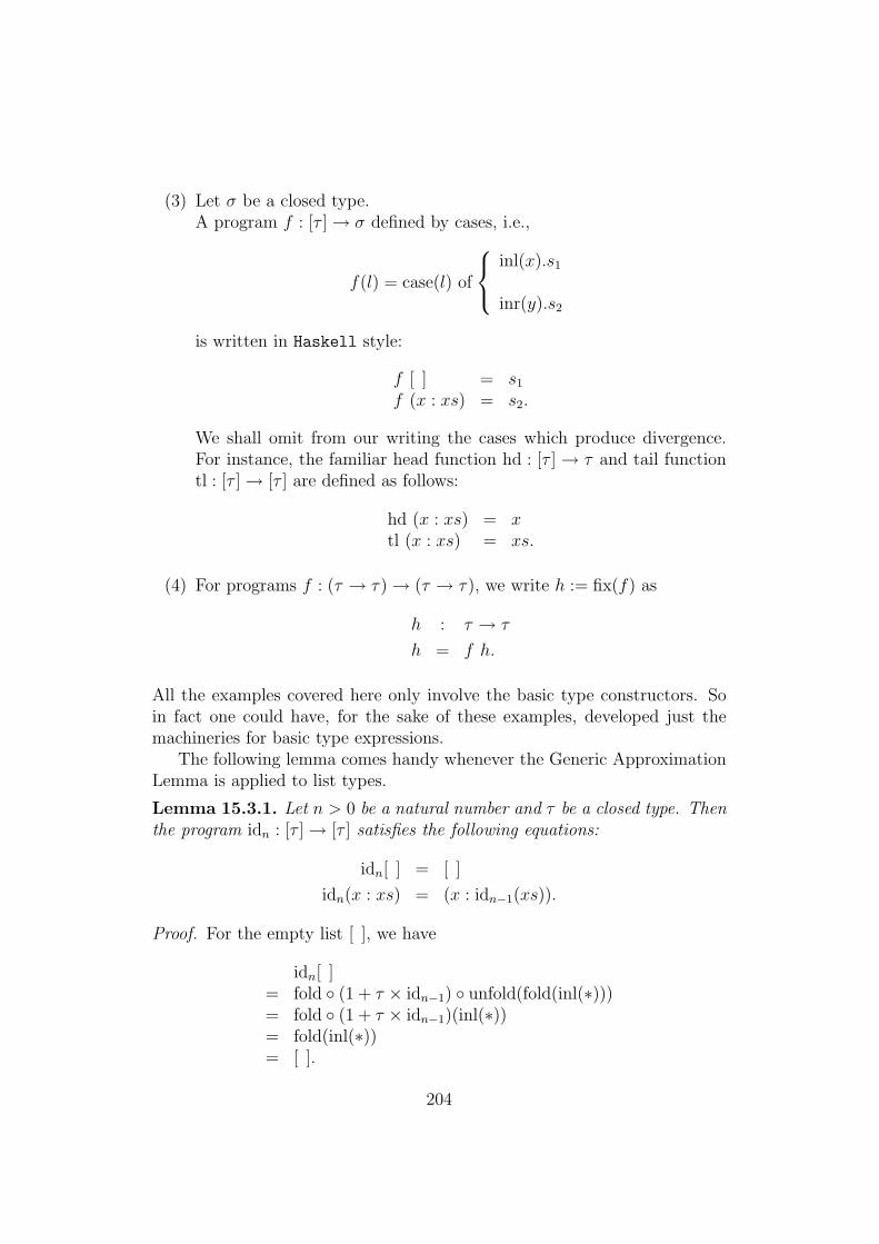
(3) Let σ be a closed type.A program f : [τ ] → σ defined by cases, i.e.,

f(l) = case(l) of

inl(x).s1

inr(y).s2

is written in Haskell style:

f [ ] = s1

f (x : xs) = s2.

We shall omit from our writing the cases which produce divergence.For instance, the familiar head function hd : [τ ] → τ and tail functiontl : [τ ] → [τ ] are defined as follows:

hd (x : xs) = xtl (x : xs) = xs.

(4) For programs f : (τ → τ) → (τ → τ), we write h := fix(f) as

h : τ → τ

h = f h.

All the examples covered here only involve the basic type constructors. Soin fact one could have, for the sake of these examples, developed just themachineries for basic type expressions.

The following lemma comes handy whenever the Generic ApproximationLemma is applied to list types.

Lemma 15.3.1. Let n > 0 be a natural number and τ be a closed type. Thenthe program idn : [τ ] → [τ ] satisfies the following equations:

idn[ ] = [ ]

idn(x : xs) = (x : idn−1(xs)).

Proof. For the empty list [ ], we have

idn[ ]= fold (1 + τ × idn−1) unfold(fold(inl(∗)))= fold (1 + τ × idn−1)(inl(∗))= fold(inl(∗))= [ ].

204

For the list (x : xs), we have

idn(x : xs)= fold (1 + τ × idn−1) unfold(fold(inr(x, xs)))= fold (1 + τ × idn−1)(inr(x, xs))= fold(inr(x, idn−1(xs)))= (x : idn−1(xs)).

15.3.2 The map-iterate property

We define two familiar functions map and iterate.map : (τ → τ) → [τ ] → [τ ]map f [ ] = [ ]map f (x : xs) = (f(x) : map f xs)

iterate : (τ → τ) → τ → [τ ]iterate f x = (x : iterate f f(x))

Proposition 15.3.2. (The map-iterate property)Let τ be a closed type. For any f : (τ → τ) and any x : τ , it holds that

map f (iterate f x) = iterate f f(x).

This property had been proven in [20] using program fusion. We repro-duce their proof here. For this method, one needs to define the programunfd as follows. Let σ and τ be given closed types. Define

unfd : (σ → Bool) → (σ → τ) → (σ → σ) → σ → [τ ]unfd p h t x = if p(x) then [ ] else h(x) : unfd p h t tx

The unfd function “encapsulates the natural basic pattern of co-recursive def-inition” (p.9 of [20]). Because several familiar co-recursive functions on listscan be defined in terms of unfd, one can rely on a universal property (whichwe describe below) of unfd to generate a powerful proof method wheneversuch co-recursive programs are involved. For example, if we define

F : σ → Bool

F x = F (:= inl(⊥))then we can define the program iterate as follows:

iterate f := unfd F id f.

Likewise, if we define

205

null : [τ ] → Bool

null [ ] = T (:= inr(⊥))null (x : xs) = F (:= inl(⊥))

then the program map can be defined as follows:

map f = unfd null (f hd) tl.

The proof method relies on a universal property enjoyed by unfd, which wenow describe. Define q : σ → 1 + τ × σ by

q(x) = if p(x) then inl(∗) else inr(h(x), t(x))

and k : σ → [τ ] byk = unfd p h t.

It then follows from the definitions of q and k that the diagram

σq

- 1 + τ × σ

[τ ]

k

?

unfold[τ ]- 1 + τ × [τ ]

1 + idτ × k

?

commutes. Moreover k = unfd p h t is the unique morphism making theabove diagram commute since unfold[τ ] : [τ ] → 1+τ×[τ ] is a final (1+τ×−)-coalgebra by Theorem 14.1.2. Further suppose that p′ : σ → Bool, h′ : σ → τand t′ : σ → σ are programs such that

p′ = p g, h′ = h g and g t′ = t g.

By defining q′(x) = if p′(x) then inl(∗) else inr(h′(x), t′(x)), it follows that

206

the upper quadrangle

σq′

- 1 + τ × σ

σq

-

g

-

1 + τ × σ

1 +τ×

g

[τ ]

k g

?

unfold[τ ]-

k

1 + τ × [τ ]

1 + τ × (k g)

?

1 +τ ×

k -

commutes. Notice that the finality of unfold[τ ] : [τ ] → 1 + τ × [τ ] guaranteesthat k g is the unique map such that the outer quadrangle of the abovediagram commutes. Thus, the following inference rule holds:

p g = p′ h g = h′ t g = g t′

(unfd p h t) g = unfold p′ h′ t′.

This rule states three conditions which together ensure that the compositionof an unfd and a function can be fused together to give a single unfd.

It follows from the above inference rule that

(unfd p h t) t = unfd (p t) (h t) t (15.1)

map f (unfd p h t) = unfd p (f h) t (15.2)

207

Proof.(iterate f) f

= (unfd F id f) f (def. of iterate)= unfd (F f) (id f) f (fusion (15.1))= unfd F (f id) f (constant functions, composition)= map f unfd F id f (fusion (15.2))= map f iterate f. (def. of iterate)

Remark 15.3.3. Program fusion is a high-level method, i.e., it allows proofsto be performed in a purely equational way. However, it is too specialiseda method in that programs involved must first be encoded using the unfdfunction.

We prove the Map-Iterate Proposition 15.3.2 using Corollary 15.2.2.

Proof. We prove by induction on n that for any x : τ and any f : (τ → τ) itholds that

map f (iterate f x) =n iterate f f(x).

The base case is trivial and the inductive step is justified by:idn+1(map f (iterate f x))

= idn+1(map f (x : iterate f f(x))) (def. of iterate)= idn+1(f(x) : map f (iterate f f(x))) (def. of map)= f(x) : idn(map f (iterate f f(x))) (Lemma 15.3.1)= f(x) : idn(iterate f f(f(x))) (Ind. hyp.)= idn+1(f(x) : iterate f f(f(x))) (Lemma 15.3.1)= idn+1(iterate f f(x)) (def. of iterate)

Thus the result holds by Corollary 15.2.2.

15.3.3 Zipping two natural number lists

Let us define some programs.zip : [σ] → [τ ] → [σ × τ ]zip [ ] l = [ ]zip (x : xs) [ ] = [ ]zip (x : xs) (y : ys) = (x, y) : zip xs ysfrom : Nat→ Nat→ [Nat]from x y = (x : from (x + y) y)

succ : Nat→ Nat

succ x = x + 1

208

We use the following notation:

succ0 = idNat and succi+1 = succ succi.

plus : (Nat× Nat) → Nat

plus (x, y) = if x == 0 then y else 1 + plus(x− 1, y)Note that plus(x, y) = x + y.

For each natural number k, define:natsk : [Nat]natsk = (k : map succ natsk)

Proposition 15.3.4. For any positive integer k, it holds that:

map plus (zip natsk natsk) = from 2k 2.

In Pitts [41], the above proposition is established using Kleene equiva-lence and list-bisimulations. Before we reproduce his proof, let us recall thedefinition of list-bisimulation (cf. Pitts [41]), a technique used for provingcontextual equivalence of lists.

Proposition 15.3.5. (List-bisimulation, Proposition 3.10 of [41])For any type τ , a binary relationR ⊆ Exp[τ ]×Exp[τ ] is called a [τ ]-bisimulationif whenever l R l′

l ⇓ [ ] =⇒ l′ ⇓ [ ] (15.3)

l′ ⇓ [ ] =⇒ l ⇓ [ ] (15.4)

l ⇓ (x : xs) =⇒ ∃x′, xs′. (15.5)

(l′ ⇓ (x′ : xs′) ∧ x =τ x′ ∧ xs R xs′)

l′ ⇓ (x′ : xs′) =⇒ ∃x, xs. (15.6)

(l ⇓ (x : xs) ∧ x =τ x′ ∧ xs R xs′).

Then for any l, l′ : [τ ],

l =[τ ] l′ iff l R l′ for some [τ ]-bisimulation R .

Proof. (=⇒): Since contextual equivalence is a bisimulation, it follows fromTheorem 7.4.4 that =[τ ] satisfies the condition (bis 5). Using this, we canprove that

(l, l′)|l =[τ ] l′

is a [τ ]-bisimulation. The details are as follows:

209

(1) Suppose l ⇓ [ ] and l =[τ ] l′. We must show that l′ ⇓ [ ]. Recallthat [ ] := fold(inl(∗)). By the evaluation rule (⇓ unfold), we deducethat unfold(l) ⇓ inl(∗). Now by (bis 5) we have that unfold(l) =1+τ×[τ ]

unfold(l′). It then follows from (bis 3a)that unfold(l′) ⇓ inl(∗′) forwhere ∗ =1 ∗′. Thus by (⇓ unfold) again, we have l′ ⇓ fold(inl(∗′)), i.e.,l′ ⇓ [ ]. Hence (15.3) holds. Similarly, (15.4) holds.

(2) Suppose that l ⇓ (x : xs) and l =[τ ] l′. We must show that there existx′ : τ and xs′ : [τ ] such that x =τ x′ and xs =[τ ] xs′. Recall that(x : xs) := fold(inr(x, xs)). It follows from (⇓ unfold) that unfold(l) ⇓inr(x, xs). By (bis 5), it follows that unfold(l) =1+τ×[τ ] unfold(l′). Itthen follows that from (bis 3b) that unfold(l′) ⇓ inr(x′, xs′) for somex′, xs′ with x =τ x′ and xs =[τ ] xs′. By (⇓ unfold), we have thatl′ ⇓ fold(inr(x′, xs′)). Thus (15.5) holds. Similarly, so does (15.6).

(⇐=): Given a [τ ]-bisimulation R, construct a relation R′ ⊆ Exp1+τ×[τ ] ×Exp1+τ×[τ ] as follows:

t R′ t′ def⇔ (t ⇓ inl(∗) =⇒ t′ ⇓ inl(∗)) ∧(t′ ⇓ inl(∗) =⇒ t ⇓ inl(∗)) ∧(∀x : τ, xs : [τ ].t ⇓ inr(x, xs) =⇒∃x′ : τ, xs′ : [τ ].t′ ⇓ inr(x′, xs′) ∧ x =τ x′ ∧ xs R xs′) ∧

(∀x′ : τ, xs′ : [τ ].t′ ⇓ inr(x′, xs′) =⇒∃x : τ, xs : [τ ].t ⇓ inr(x, xs) ∧ x =τ x′ ∧ xs R xs′)

The fact that contextual equivalence satisfies the conditions of a bisimulationand that R satisfies (15.3) - (15.6) together imply that

Bσ:=

R ∪(l, l′)|l =[τ ] l′ if σ = [τ ]

R′ ∪(t, t′)|t =1+τ×[τ ] t′ if σ = 1 + τ × [τ ]

(t, t′)|t =σ t′ otherwise

defines an FPC bisimulation. Thus if l R l′, then l B[τ ] l′ and so l =[τ ] l′ byTheorem 7.4.4.

We reproduce Pitts’ proof of Proposition 15.3.4 which uses Proposition15.3.5.

Proof. Consider the following closed terms defined by induction on n ∈ N:

n0 := k e0 := 2k l0 := natsk

nm+1 := succ nm em+1 := em + 2 lm+1 := map succ lm

210

The definitions of from and em bear upon us to have:

from em 2 ⇓ (em : from em+1 2) (15.7)

From the definitions of map, natsk, lm and nm, it follows by induction on mthat

lm ⇓ (nm : lm+1)

By applying the zip function, we have that

zip lm lm ⇓ ((nm, nm) : zip lm+1 lm+1)

and from the definition of map that

map plus (zip lm lm) ⇓ (plus (nm, nm) : map plus (zip lm+1 lm+1)) (15.8)

One then establishes routinely by induction on m that

plus (nm, nm) ∼=kl em

and thus by Proposition 7.5.1 we have

plus (nm, nm) =Nat em. (15.9)

Now define R ⊆ [Nat]× [Nat] by

R:= (map plus (zip lm lm)), from em 2|m ∈ N.

Then properties (15.7) - (15.9) together implies that R satisfies all the con-ditions (15.3)-(15.6) and hence is a [Nat]-bisimulation. Thus the proof iscomplete by virtue of Proposition 15.3.5.

Remark 15.3.6. Notice that in order to apply Proposition 15.3.5 one mustcome up with a suitable list-bisimulation.

Before using Corollary 15.2.2 to prove Proposition 15.3.4, we establish auseful property.

Proposition 15.3.7. For any i, k ∈ N, it holds that

map succi+1 natsk = map succi natsk+1.

Proof. We prove by induction on n that for all i, k ∈ N,

map succi+1 natsk =n map succi natsk+1.

211

and the desired result follows from Corollary 15.2.2. The base case is trivialand the inductive step is justified by

idn+1(map succi+1 natsk)= idn+1(map succi+1 (k : map succ natsk))= idn+1(succi+1(k) : map succi+1(map succ natsk))= idn+1(succi+1(k) : map succi+2 natsk)= (succi+1(k) : idn(map succi+2 natsk))= (succi+1(k) : idn(map succi+1 natsk+1)) (ind. hyp.)= (succi(k + 1) : idn(map succi(map succ natsk+1)))= idn+1(map succi (k + 1 : map succ natsk+1))= idn+1(map succi natsk+1)

We now prove Proposition 15.3.4 using Corollary 15.2.2.

Proof. We prove by induction on n that for all k ∈ N, it holds that

map plus (zip natsk natsk) =n from 2k 2.

The base case is trivial and the inductive step is justified by:idn+1(map plus (zip natsk natsk))

= idn+1(map plus((k, k) : zip (map succ natsk) (map succ natsk))))

= idn+1(2k : map plus(zip (map succ natsk) (map succ natsk)))

= idn+1(2k : map plus (zip natsk+1 natsk+1))= (2k : idn(map plus (zip natsk+1 natsk+1)))= (2k : idn(from 2k + 2 2))= idn+1(2k : from 2k + 2 2)= idn+1(from 2k 2)

The desired result then follows from Corollary 15.2.2.

15.3.4 The ‘take’ lemma

Let us now define the take function of Bird & Wadler [8].take : Nat→ [τ ] → [τ ]take 0 l = [ ]take n [ ] = [ ]take n (x : xs) = (x : take n− 1 xs)

212

Proposition 15.3.8. (The ‘take’ lemma)Let τ be a closed type and l, l′ : [τ ].

∀n ∈ N.(take n l =[τ ] take n l′) =⇒ l =[τ ] l′.

We reproduce Pitts’ proof (cf. [41] of Proposition 15.3.8 which uses Propo-sition 15.3.5.

Proof. For a given type τ , define R ⊆ Exp[τ ] × Exp[τ ] by:

R:= (l, l′)|∀n ∈ N(take n l =[τ ] take n l′.

We prove that R satisfies conditions (15.3) - (15.6). First of all, by theevaluation rules and Kleene equivalence, the following properties hold: Forall n ∈ N, x : τ and l, xs : [τ ],

(a) take n + 1 l ⇓ [ ] ⇐⇒ l ⇓ [ ].

(b) take n + 1 l ⇓ (x : xs) ⇐⇒ ∃xs′.(l ⇓ (x : xs′) ∧ xs =[τ ] take n xs′).

Now suppose that l R l′, i.e., ∀n ∈ N.take n l = take n l′.

(1) To establish condition (15.3), we suppose that l ⇓ [ ]. Then (a) impliesthat take 1 l ⇓ [ ]. Since l R l′, by definition ofR, take 1 l =[τ ] take 1 l′.Since contextual equivalence is an FPC bisimulation, it follows thattake 1 l′ ⇓ [ ]. Hence by (a) again, it holds that l′ ⇓ [ ].

(2) A symmetrical argument shows that R satisfies condition (15.4).

(3) To see that it satisfies condition (15.5), suppose l ⇓ (x : xs). Then by(b) for any n ∈ N we have take n + 1 l ⇓ (x : take n xs). Since l R l′,by definition of R, take n + 1 l =[τ ] take n + 1 l′. So since contextualequivalence is an FPC bisimulation, it follows that there are terms x′

and xs′′ with

take n + 1 l′ ⇓ (x′ : xs′′) ∧ x =τ x′ ∧ take n xs =[τ ] xs′′.

By (b) again, l′ ⇓ (x′ : xs′) for some xs′ with xs′′ =[τ ] take n xs′. Weneed finally to verify that xs R xs′. But note that for all n we havetake n xs =[τ ] xs′′ =[τ ] take n xs′. Thus we conclude that

∀n ∈ N.(take n xs =[τ ] take n xs′).

(4) A symmetrical argument shows that R also satisfies condition (15.6).

213

Thus R is a [τ ]-bisimulation. In particular, we have that R is a bisimulationand so the required contextual equivalence is obtained.

Let us now provide an alternative proof of Proposition 15.3.8 by usingCorollary 15.2.2.

Proof. We prove by induction on m that for all l, l′ ∈ [τ ], it holds that

∀n ∈ N.(take n l =[τ ] take n l′) =⇒ l =m l′.

The base case is trivial and we proceed to the induction step.Assume that the statement holds for the natural number m, we want to provethat it holds for m + 1.Case 1: l =[τ ] [ ]Since take 1 l =[τ ] take 1 l′ =[τ ] [ ], it follows that l′ =[τ ] [ ], for otherwise ifl′ =[τ ] (x : xs) it would have been the case that take 1 l′ =[τ ] (x : [ ]) 6=[τ ] [ ].Thus we have l =m+1 l′ trivially.Case 2: l =[τ ] (x : xs)In that case, l′ =[τ ] (y : ys) for some terms y and ys. Again by applyingtake 1 to both the list, we have that x =τ y. Now assume for the purpose ofinduction that l =m l′. Note that

idm+1(l) =[τ ] idm+1(x : xs)

=[τ ] (x : idm(xs))

=[τ ] (y : idm(xs)).

Since l =[τ ] (x : xs) and l′ =[τ ] (y : ys), it holds that

∀n ∈ N.take n (x : xs) =[τ ] take n (y : ys).

This implies that∀n ∈ N.take n xs =[τ ] take n ys.

The induction hypothesis then asserts that xs =m ys. Thus idm+1(l) =[τ ]

(y : idm(xs)) =[τ ] (y : idm(ys)) =[τ ] idm+1(l′), i.e., l =m+1 l′.

15.3.5 The filter-map property

The next sample application involves the filter function, which we definebelow.filter : (τ → Bool) → ([τ ] → [τ ])filter u [ ] = [ ]filter u (x : xs) = if u(x) then (x : filter u xs) else filter u xs

214

Proposition 15.3.9. For any u : (τ → Bool), v : (τ → τ) and l : [τ ], itholds that

filter u (map v l) =[τ ] map v (filter (u v) l).

This proposition was established in Pitts [41] based on an induction onthe depths of proofs of evaluation. Here we elaborate. Define the nth levelevaluation relation ⇓n (written as x ⇓n v) as follows. Replace in the axiomsand rule regarding ⇓ (see Figure 4.3) each occurrence of ⇓ by ⇓n in an axiomor the premise of a rule and replacing ⇓ by ⇓n+1 in the conclusion of eachrule. Then of course we have:

x ⇓ v ⇔ ∃n ∈ N.(x ⇓n v) (15.10)

It suffices to show that there is a list bisimulation that relates filter u (map v l)and map v (filter (u v) l). Usually it is Hobson’s choice.

Proof. Define

R:= (filter u (map v l), map v (filter (u v) l))|l : [τ ].

Instead of proving the three conditions of a list bisimulation directly, wededuce them via (15.10), using the properties of ⇓n:

(1) ∀l.(filter u (map v l) ⇓n [ ] =⇒ map v (filter (u v) l ⇓ [ ]).

(2) ∀l.(map v (filter (u v) l ⇓n [ ] =⇒ filter u (map v l) ⇓ [ ]).

(3) ∀l, x, xs.(filter u (map v l) ⇓n (x : xs) =⇒∃xs′.(map v (filter (u v) l) ⇓ (x : xs′) ∧ xs R xs′).

(4) ∀l, x, xs′.(map v (filter (u v) l) ⇓n (x : xs′) =⇒∃xs.(filter u (map v l) ⇓ (x : xs) & xs R xs′).

The proofs of (1) - (4) are by induction on n.

We now prove Proposition 15.3.9 by using Corollary 15.2.2.

Proof. Given any l : [τ ], we have two possibilities:

(1) There is n ∈ N such that tl(n)(l) =[τ ] [ ].

(2) For all n ∈ N, tl(n)(l) 6=[τ ] [ ].

215

Here tl(0)(l) := l and tl(n+1)(l) := tl(tl(n)(l)).Those lists which satisfy (1) are called finite lists. For a finite list, we defineits length to be n ∈ N for which tl(n)(l) =[τ ] [ ]. Those lists which satisfy (2)are called infinite lists.We prove Proposition 15.3.9 for each of these cases.

(1) Finite listsWe prove by induction on the length of finite lists that

filter u (map v l) =[τ ] map v (filter (u v) l).

Base case: n = 0.In this case, l =[τ ] [ ]. On one hand, we have:

filter u (map v l) ≡ filter u (map v [ ])

=[τ ] filter u [ ]

=[τ ] [ ]

On the other hand, we have:

map v (filter (u v) l) ≡ map v (filter (u v) [ ])

=[τ ] map v [ ]

=[τ ] [ ]

Hence the statement holds.Inductive step:Assume that the statement holds for all finite lists of length n. We wantto prove that the statement holds for all finite lists of length n+1. Wewrite l = (x : xs).

filter u (map v l) ≡ filter u (map v (x : xs))

=[τ ] filter u (v(x) : map v xs)

=[τ ]

filter u (map v xs) if u v(x) = F

(v(x) : filter u (map v xs)) if u v(x) = T

Ind. hyp.=[τ ]

map v (filter (u v) xs) if u v(x) = F

(v(x) : map v (filter (u v) xs)) if u v(x) = T

(2) Infinite lists

216

We prove by induction on m that for all infinite lists l

filter u (map v l) =m map v (filter (u v) l).

Base case: m = 0. This holds trivially.Inductive step: There are two possibilities:(i) u v(hd(tl(n)(l))) =[τ ] F for all n ∈ N.Since the evaluations of filter u (map v l) and map v (filter (u v) l)involve infinite unfoldings, it follows that both diverges. Hence thestatement holds.(ii) There is a minimum n ∈ N such that u v(hd(tl(n)(l))) =[τ ] T.Then we have:

idm+1(filter u (map v l))

=[τ ] idm+1(filter u (map v tl(n)(l))) (Kleene equiv.)

=[τ ] idm+1(v(hd(tl(n)(l))) : filter u (map v tln+1(l))) (map & filter)

=[τ ] (v(hd(tl(n)(l))) : idm(filter u (map v tln+1(l)))) (Lemma 15.3.1)

=[τ ] (v(hd(tl(n)(l))) : idm(map v (filter (u v) tln+1(l)))) (Ind. hyp.)

=[τ ] idm+1(v(hd(tl(n)(l))) : map v (filter (u v) tln+1(l))) (Lemma 15.3.1)

=[τ ] idm+1(map v filter (u v) tl(n)(l)) (map & filter)=[τ ] idm+1(map v (filter (u v) l)). (Kleene equiv.)

The desired result then follows from Corollary 15.2.2.

217

Part V

Conclusion

218

In this part, we make some concluding remarks regarding the presentresearch. In Chapter 16, we state some problems which we have encounteredduring the course of the research and which at the time of writing still remainsopen. Also we describe some possible work which may be carried out in thefuture. In Chapter 17, we give a summary of the contributions made in thisthesis.

219

Chapter 16

Open problems and future work

In this chapter, we describe some open problems encountered in the courseof our present work. In addition, we briefly explore future areas of work.

16.1 An operational proof of the minimal in-

variance property

In Chapter 13, we have employed a domain-theoretic denotational semanticsto establish an operational minimal invariance property, i.e., Lemma 13.3.7.A natural question is whether this can be proven by purely operational meth-ods. In the existing literature, Lassen [33] and Birkedal & Harper [9] containan operational proof of a ‘syntactic minimal invariance property’. However,as noted in Chapter 1, the language considered in these works only dealwith one top-level recursive type. In what follows, we give an outline of onepossible1 adaption of Birkedal & Harper’s method.

16.1.1 Functoriality

Recall that in Chapter 13, we can view FPC expressions as realisable func-tors. Since we wish to establish a purely operational proof of the operationalminimal invariance property, we do not assume that FPC expressions pre-serve identity morphisms.

By the same construction in Section 13.3 , all FPC type expressions almostdefine realisable functors: all properties of functors hold except that we are

1The other possibility that may work is to adapt Lassen’s relational reasoning aboutcontexts [33]. Unfortunately, this reference is only known to the author very near thecompletion of the present writing.

220

not able to establish preservation of identities. We refer to such gadgets assemi-functors.

Although we have yet to show that the semi-functors associated to FPCtypes-in-context are indeed functors, we can say something about their actionon the identities.

Lemma 16.1.1. For every type-in-context Θ ` τ , the realisable semi-functorTΘ`τ associated to it satisfies the following property:For every sequence of closed types ~σ, it holds that

TΘ`τ (id~σ : ~σ ~σ : id~σ) v (idTΘ`τ (~σ), idTΘ`τ (~σ)).

Proof. By a straightforward induction on the structure of Θ ` σ.

What we have been unable to show at the time of writing is that theopposite inequality also holds. We elaborate a possible proof strategy inSection 16.1.6. We first need some technical material developed in the nextsection.

16.1.2 Pre-deflations revisited

Recall that in Chapter 15, we defined a type-indexed family of pre-deflationsdσ : ω → (σ → σ). In particular, for the clause concerning recursive types,we abuse notation by writing Π2S(dµX.σ(n), dµX.σ(n)) as S(dµX.σ(n)) anddefine

dµX.σ(n)(x) := if (n > 0) then fold S(dµX.σ(n− 1)) unfold(x).

Note that:

dµX.σ(0) = ⊥µX.σ→µX.σ

dµX.σ(n + 1) = fold S(dµX.σ(n)) unfold.

If one define the program Φ : (µX.σ → µX.σ) → (µX.σ → µX.σ) byΦ(u, v) := (unfold, fold) TX`σ (fold, unfold), then it is clear that

Φ(n)(⊥,⊥) = (dµX.σ(n), dµX.σ(n)).

Notice that establishing the operational minimal invariance property is equiv-alent to establishing that

fix(Φ) = (idµX.σ, idµX.σ).

221

In order to prove this, we propose to show that

dµX.σ(∞) = idµX.σ.

It is easy to show that dµX.σ(∞) v idµX.σ. In fact, we can do better.

Lemma 16.1.2. For every closed type σ and every n : ω, the standard pre-deflation dσ(n) : σ → σ is

(1) below the identity idσ, and

(2) idempotent.

Proof. By induction on the structure of σ. The proof is fairly routine but thereader may want to note how part (1) is established for the recursive types.To do this, we have to prove by a further induction on n that

dµX.σ(n) v idµX.σ.

(n = 0): This is trivial since dµX.σ(0) = ⊥ v id.(n+1): Abusing notations, one may proceed as follows:

dµX.σ(n + 1) = fold TX`σ(dµX.σ(n)) unfold

v fold TX`σ(idµX.σ) unfold

v fold idµX.σ unfold

= idµX.σ

where the first v holds by induction hypothesis and the second v holdsbecause of Lemma 16.1.1.

So in order to prove the operational minimal invariance property, it suf-fices to show that

idµX.σ v dµX.σ(∞).

Before we proceed to the next subsection, we establish the following result.

Lemma 16.1.3. Let ~X ` σ be a type-in-context. Then the semi-functorS ~X`σ satisfies the following (contextual) inequality.:

S ~X`σ(dτ1(∞), . . . , dτn(∞)) v dσ[~τ/ ~X](∞)

for any sequence of closed types ~τ .

Proof. By induction on the structure of ~X ` σ.

222

In order that the proof strategy of Birkedal & Harper [9] works for ourlanguage, we invoke the following conjecture.

Conjecture 16.1.4. For every type-in-context of the form X ` σ, it holdsthat

dµX.σ(∞) fold = fold dσ[µX.σ/X](∞).

We have yet to establish this conjecture, though in many instances (e.g.list-type) this conjecture holds trivially. Notice that if we can establish theother inequality in Lemma 16.1.3, i.e.,

S ~X`σ(dτ1(∞), . . . , dτn(∞)) w dσ[~τ/ ~X](∞)

holds for any sequence of closed types ~τ , then Conjecture 16.1.4 follows.However, a proof of the above inequality evades us at the time of writing.

In what follows, we show how an operational proof of Lemma 13.3.7 canbe obtained assuming this conjecture. This conjecture is invoked only onceand we indicate clearly where this takes place.

16.1.3 Compilation relation

One important tool which Birkedal & Harper use in their operational proofof the ‘syntactic minimal invariance’ (Theorem 3.66 of [9]) is the compilationrelation⇒. In this section, we define and prove several elementary propertiesregarding this relation.

The compilation relation on Expσ(Γ) is defined by induction on the deriva-tion of Γ ` t : σ, given by the axioms and rules in Figure 16.1.

The compilation relation ⇒ turns out to be a function.

Proposition 16.1.5. If Γ ` t : σ, then Γ ` t : σ ⇒ |t| for some unique|t| ∈ Expσ(Γ).

Proof. By induction on the derivation of Γ ` t : σ.

Lemma 16.1.6. If Γ ` t : σ ⇒ |t|, then Γ ` dσ(∞)(|t|) =σ |t|.

Proof. By induction on the derivation of Γ ` t : σ ⇒ |t|.The cases for (⇒ var), (⇒ pair), (⇒ inl), (⇒ inr), (⇒ abs), (⇒ up) and (⇒fold) rely on the idempotence of d(∞) (cf. Lemma 16.1.2 without having toinvoke the induction hypothesis. We show the case for (⇒ var) here.Given that Γ ` x : σ ⇒ |x|. By definition, |x| = dσ(∞)(x). We are to showthat Γ ` dσ(∞)|x| = |x|. But this follows from the idempotence of dσ(∞),i.e., Γ ` dσ(∞)|x| =σ dσ(dσ(x)) =σ dσ(x) = |x|.

223

Γ ` x : σ ⇒ dσ(∞)(x)(if x ∈ dom(Γ)) (⇒ var)

Γ ` s : σ ⇒ |s| Γ ` t : τ ⇒ |t|Γ ` (s, t) : σ × τ ⇒ dσ×τ (∞)(|s|, |t|) (⇒ pair)

Γ ` p : σ × τ ⇒ |p|Γ ` fst(p) : σ ⇒ fst(|p|) (⇒ fst)

Γ ` p : σ × τ ⇒ |p|Γ ` snd(p) : τ ⇒ snd(|p|) (⇒ snd)

Γ ` s : σ ⇒ |s|Γ ` inl(s) : σ + τ ⇒ dσ+τ (∞)(inl(|s|)) (⇒ inl)

Γ ` s : τ ⇒ |s|Γ ` inr(s) : σ + τ ⇒ dσ+τ (∞)(inr(|s|)) (⇒ inl)

Γ ` s : σ + τ ⇒ |s| Γ, x : σ ` t1 : ρ ⇒ |t1| Γ, y : τ ` t2 : ρ ⇒ |t2|Γ ` case(s) of inl(x).t1 or inr(y).t2 : ρ ⇒ case(|s|) of inl(x).|t1| or inr(y).|t2|

(⇒ case)

Γ ` s : σ → τ ⇒ |s| Γ ` t : σ ⇒ |t|Γ ` s(t) : τ ⇒ |s|(|t|) (⇒ app)

Γ, x : σ ` t : τ ⇒ |t|Γ ` λxσ.t : σ → τ ⇒ dσ→τ (∞)(λx.|t|) (⇒ abs)

Γ ` t : σ ⇒ |t|Γ ` up(t) : σ⊥ ⇒ dσ⊥(∞)(|t|) (⇒ up)

Γ ` s : σ⊥ ⇒ |s| Γ, x : σ ` t : ρ ⇒ |t|Γ ` case(s) of up(x).t : ρ ⇒ case(|s|) of up(x).|t| (⇒ case up)

Γ ` t : µX.σ ⇒ |t|Γ ` unfold(t) : σ[µX.σ/X] ⇒ unfold(|t|) (⇒ unfold)

Γ ` t : σ[µX.σ/X] ⇒ |t|Γ ` fold(t) : µX.σ ⇒ dµX.σ(∞)(fold(|t|)) (⇒ fold)

Figure 16.1: Definition of Γ ` t : σ ⇒ |t|

224

The rest of the cases are fairly routine except for the case (⇒ unfold) whichwe now show.Let Γ ` unfold(t) : σ[µX.σ/X] ⇒ |unfold(t)| be given. We must show that

Γ ` dσ[µX.σ/X](∞)|unfold(t)| =σ[µX.σ/X] |unfold(t)|.

The inference rule (⇒ unfold)

Γ ` t : µX.σ ⇒ |t|Γ ` unfold(t) : σ[µX.σ/X] ⇒ unfold(|t|)

guarantees that |unfold(t)| ≡ unfold(|t|). The induction hypothesis assertsthat Γ ` dµX.σ(|t|) =µX.σ |t|. It then follows that

Γ ` dσ[µX.σ/X](∞)|unfold(t)|≡ dσ[µX.σ/X](∞)(unfold(|t|))w SX`σ(dµX.σ(∞)) unfold(|t|) (Lemma 16.1.3)

= unfold dµX.σ(∞)(|t|) (def. of dµX.σ(∞))= unfold(|t|) (Ind. hyp.)= |unfold(t)|.

But already, by Lemma 16.1.2, we always have dσ[µX.σ/X](∞)(|unfold(t)|) v|unfold(t)| so that

dσ[µX.σ/X](∞)(|unfold(t)|) = |unfold(t)|.

Lemma 16.1.7. If Γ ` t : σ ⇒ |t|, then Γ ` |t| vσ t.

Proof. By induction on Γ ` t : σ ⇒ |t|, using the previous lemma.

16.1.4 Compilation of a context

One last technical gadget is to compile a context C[−σ] ∈ Ctxτ (Γ). Fora given context C[−σ] ∈ Ctxτ (Γ), we define a compiled context |C|[−σ] ∈Ctxτ (Γ) using the axioms and rules similar to those for defining Γ ` t : σ ⇒|t|. The axioms and rules for defining |C| is given in Figure 16.2.

Lemma 16.1.8. If Γ ` t : σ ⇒ |t| and C[−σ] ∈ Ctx(Γ), then

Γ ` |C[t]| =τ |C|[|t|].

Proof. By induction on the structure of C[−σ].

225

Γ ` −σ ⇒ dσ(∞)(−σ) (⇒ par)

Γ ` x : σ ⇒ dσ(∞)(x)(if x ∈ dom(Γ)) (⇒ var)

Γ ` S : σ ⇒ |S| Γ ` T : τ ⇒ |T |Γ ` (S, T ) : σ × τ ⇒ dσ×τ (∞)(|S|, |T |) (⇒ pair)

Γ ` P : σ × τ ⇒ |P |Γ ` fst(P ) : σ ⇒ fst(|P |) (⇒ fst)

Γ ` P : σ × τ ⇒ |P |Γ ` snd(P ) : τ ⇒ snd(|P |) (⇒ snd)

Γ ` S : σ ⇒ |S|Γ ` inl(S) : σ + τ ⇒ dσ+τ (∞)(inl(|S|)) (⇒ inl)

Γ ` S : τ ⇒ |S|Γ ` inr(S) : σ + τ ⇒ dσ+τ (∞)(inr(|S|)) (⇒ inl)

Γ ` S : σ + τ ⇒ |S| Γ, x : σ ` T1 : ρ ⇒ |T1| Γ, y : τ ` T2 : ρ ⇒ |T2|Γ ` case(S) of inl(x).T1 or inr(y).T2 : ρ ⇒ case(|S|) of inl(x).|T1| or inr(y).|T2|

(⇒ case)

Γ ` S : σ → τ ⇒ |S| Γ ` T : σ ⇒ |T |Γ ` S(T ) : τ ⇒ |S|(|T |) (⇒ app)

Γ, x : σ ` T : τ ⇒ |T |Γ ` λxσ.T : σ → τ ⇒ dσ→τ (∞)(λx.|T |) (⇒ abs)

Γ ` T : σ ⇒ |T |Γ ` up(T ) : σ⊥ ⇒ dσ⊥(∞)(|T |) (⇒ up)

Γ ` S : σ⊥ ⇒ |S| Γ, x : σ ` T : ρ ⇒ |T |Γ ` case(S) of up(x).T : ρ ⇒ case(|S|) of up(x).|T | (⇒ case up)

Γ ` T : µX.σ ⇒ |T |Γ ` unfold(T ) : σ[µX.σ/X] ⇒ unfold(|T |) (⇒ unfold)

Γ ` T : σ[µX.σ/X] ⇒ |T |Γ ` fold(T ) : µX.σ ⇒ dµX.σ(∞)(fold(|T |)) (⇒ fold)

Figure 16.2: Definition of Γ ` C[−σ] : τ ⇒ |C|[−σ]

226

Lemma 16.1.9. Let C[−σ] ∈ Ctxτ (Γ) and t ∈ Expσ. Then

|C|[t] vτ C[t].

Proof. By induction on the structure of C[−σ].

16.1.5 A crucial lemma

The following lemma relies on Conjecture 16.1.4.

Lemma 16.1.10. If Conjecture 16.1.4 holds, then

(∅ ` t : σ ⇒ |t| ∧ t ⇓ v) =⇒ ∅ ` |t| =σ |v|.

Note that only the case (⇓ unfold) uses Conjecture 16.1.4.

Proof. By induction on the derivation of t ⇓ v.

(1) (⇓ can): Trivial.

(2) (⇓ fst,snd):Given that ∅ ` fst(p) : σ ⇒ |fst(p)| and fst(p) ⇓ v. We must show that∅ ` |fst(p)| = |v|. The premise of the only evaluation rule (⇓ fst) whichmatches fst(p) ⇓ v consists of

p ⇓ (s, t) s ⇓ v.

The induction hypothesis asserts that ∅ ` |p| =σ×τ |(s, t)| and ∅ `|s| =σ |v|. Based on these, one deduces that

∅ ` |fst(p)| ≡ fst(|p|) (def. of |fst(p)|)=σ fst(|(s, t)|) (Ind. hyp.)=σ fst(dσ(∞)(|s|), dτ (∞)(|t|)) (def. of |(s, t)|)=σ dσ(∞)(|s|) (β-rule (7.11))=σ |s| (Lemma 16.1.6)=σ |v|. (Ind. hyp.)

The case for (⇓ snd) is similar.

(3) (⇓ app):Given that ∅ ` s(t) ⇒ |s(t)| and s(t) ⇓ v. We must show that ∅ `|s(t)| =τ |v|. The only derivation of s(t) ⇓ v is via an application ofthe evaluation rule (⇓ app) whose premise is given by

s ⇓ λx.r r[t/x] ⇓ v.

227

The induction hypothesis asserts that ∅ ` |s| =σ→τ |λx.r| and ∅ `r[t/x] =σ |v|. Then the desired result follows from:

∅ ` |s(t)| ≡ |s|(|t|) (def. of |s(t)|)=τ |λx.r|(|t|) (Ind. hyp.)≡ (dσ→τ (∞)(λx.|r|))(|t|) (def. of |λx.r|)≡ (λx.dτ (∞) |r| dσ(∞))(|t|) (def. of dσ→τ )=τ (λx.dτ (∞) |r|)(dσ(∞)(|t|))=τ (λx.dτ (∞) |r|)(|t|) (Lemma 16.1.6)=τ dτ (∞)(|r|[|t|/x]) (β-rule 7.10)=τ dτ (∞)(|r[t/x]|) (Lemma 16.1.8)=τ dτ (∞)(|v|) (Ind. hyp.)=τ |v|. (Lemma 16.1.6)

(4) (⇓ case):Given that

∅ ` case(s) of inl(x).t1 or inr(y).t2 ⇒ |case(s) of inl(x).t1 or inr(y).t2|

and case(s) of inl(x).t1 or inr(y).t2 ⇓ v. We want to prove that

∅ ` |case(s) of inl(x).t1 or inr(y).t2| =ρ |v|.

W.l.o.g., let us assume that the following evaluation rule (⇓ case inl)derives the given evaluation:

s ⇓ inl(t) t1[t/x] ⇓ v

case(s) of inl(x).t1 or inr(y).t2 ⇓ v.

The induction hypothesis asserts that

∅ ` |s| =σ+τ |inl(t)| and ∅ ` |t1[t/x]| ⇓ v.

It then follows that

∅ ` |case(s) of inl(x).t1 or inr(y).t2|≡ case(|s|) of inl(x).|t1| or inr(y).|t2| (by def.)=ρ case(inl(|t|)) of inl(x).|t1| or inr(y).|t2| (Ind. hyp.)=ρ |t1|[|t|/x] (Kleene equivalence)=ρ |t1[t/x]| (Lemma 16.1.8)=ρ |v|. (Ind. hyp.)

228

(5) (⇓ case up):Given that ∅ ` case(s) of up(x).t ⇒ |case(s) of up(x).t| andcase(s) of up(x).t ⇓ v. We want to prove that

∅ ` |case(s) of up(x).t| =ρ |v|.

The premise of the evaluation rule which derives case(s) of up(x).t ⇓ vconsists of

s ⇓ up(t′) t[t′/x] ⇓ v.


|s| =σ⊥ |up(t′)| and |t[t′/x]| =ρ |v|.

The desired result then follows from

∅ ` |case(s) of up(x).t|≡ case(|s|) of up(x).|t| (def. of |case(s) of up(x).t|)=ρ case(|up(t′)|) of up(x).|t| (Ind. hyp.)=ρ case(up(|t′|)) of up(x).|t| (def. of |up(t′)|)=ρ |t|[|t′|/x] (Kleene equivalence)=ρ |t[t′/x]| (Lemma 16.1.8)=ρ |v|. (Ind. hyp.)

(6) (⇓ unfold):Given that ∅ ` unfold(t) ⇒ |unfold(t)| and unfold(t) ⇓ v. We mustshow that

∅ ` |unfold(t)| =σ[µX.σ/X] |v|.

The premise of the evaluation rule which derives unfold(t) ⇓ v consistsof

t ⇓ fold(s) s ⇓ v.


∅ ` |t| =µX.σ |fold(s)| and ∅ ` |s| =σ[µX.σ/X] |v|.

229

The desired result follows from

∅ ` |unfold(t)|≡ unfold(|t|) (def. of |unfold(t)|)=σ[µX.σ/X] unfold(|fold(s)|) (Ind. hyp.)≡ unfold(dµX.σ(∞)(fold(|s|))) (def. of |fold(s)|)=σ[µX.σ/X] unfold fold dσ[µX.σ/X](∞)(|s|) (Conjecture 16.1.4)=σ[µX.σ/X] unfold(fold(|s|)) (Lemma 16.1.6)=σ[µX.σ/X] |s| (β-rule (7.15))=σ[µX.σ/X] |v|. (Ind. hyp.)

16.1.6 Incomplete proof of functoriality

In this subsection, we present an operational proof of Lemma 13.3.7 assumingthat Conjecture 16.1.4 holds. Note that the only use of Conjecture 16.1.4occurs in Lemma 16.1.10 above.

Lemma 16.1.11. Let f, g ∈ ExpµX.σ→µX.σ be given. Suppose that for all t ∈Expσ[µX.σ/X] and for all contexts of the form C[−µX.σ→µX.σ(fold(t))] ∈ CtxΣ

it holds thatC[f(fold(t))] vΣ C[g(fold(t))].

Then f vµX.σ→µX.σ g.

Proof. By the extensionality property (7.22), in order to prove that f v g,it suffices to prove that for all s ∈ ExpµX.σ, f(s) vµX.σ g(s) holds. Lets ∈ ExpµX.σ be given and suppose C[−µX.σ] ∈ CtxΣ is such that C[f(s)] ⇓ >.Because of η-rule (7.27), it follows from the definition of v that

C[f(s)] ⇓ > ⇐⇒ C[f(fold(unfold(s)))] ⇓ >.

Thus by assumption that C[f(fold(t))] vΣ C[g(fold(t))] for all t ∈ Expσ[µX.σ/X],it follows (by defining t := unfold(s)) that C[g(fold(unfold(s)))] ⇓ >. Againinvoking η-rule (7.27) and the definition of v, we have that C[g(s)] ⇓ >, asrequired.

Lemma 16.1.12. If Conjecture 16.1.4 holds, then for any type-in-context ofthe form X ` σ, we have

∅ ` idµX.σ v dµX.σ(∞).

The conjecture is invoked via Lemma 16.1.10.

230

Proof. By Lemma 16.1.11, it suffices to show that for any t ∈ Expσ[µX.σ/X]

and for any context C[−µX.σ→µX.σ(fold(t))] ∈ CtxΣ, it holds that

C[idµX.σ(fold(t))] vΣ C[dµX.σ(∞)(fold(t))].

Let C[−µX.σ→µX.σ](fold(t))] ∈ CtxΣ be arbitrary. Since idµX.σ(fold(t)) =µX.σ

fold(t) holds (an instance of Kleene equivalence), it suffices to prove that

C[fold(t)] vΣ C[dµX.σ(∞)(fold(t))].

By Lemma 16.1.7, it suffices to show that

C[fold(t)] vΣ C[dµX.σ(∞)(|fold(t)|)].

But by Lemma 16.1.6, it suffices to show that

C[fold(t)] vΣ C[|fold(t)|].

By Lemma 16.1.10, C[fold(t)] ⇓ > implies that |C[fold(t)]| = |>| =Σ >. Itthen follows that

C[fold(t)] ⇓ > =⇒ |C[fold(t)]| ⇓ > (Lemma 16.1.10)=⇒ |C|[|fold(t)|] ⇓ > (Lemma 16.1.8)=⇒ C[|fold(t)|] ⇓ >. (Lemma 16.1.9)

which is what we aim to show.

This and Lemma 16.1.2 establish functoriality, assuming Conjecture 16.1.4.

16.2 SFP structure on FPC closed types

The careful reader would have noticed that the pre-deflationary structure isnot an SFP-structure in that the standard pre-deflations do not have finiteimages modulo contextual equivalence. To see this, just take the case oflist-types, e.g. [τ ]. The pre-deflation at precision n is given by

d[τ ]n (x : xs) = (x : d

[τ ]n−1(xs)).

Because τ may have an infinite number of elements (mod contextual equiv-alence), it is clear that d[τ ] does not have a finite image modulo contextualequivalence. The question is whether it is possible to derive an SFP-structureon FPC closed types by defining families of SFP-deflations. At the time ofwriting, it is not known whether FPC types are SFP.

231

One possible way is to replace in the definition of standard pre-deflationsthe clause concerning recursive types by:

dµX.σ(n) := if n > 0 then fold dσ[µX.σ/X](n− 1) unfold.

This is not a recursive definition of the form fix(t) for some suitable term tbecause it involves the type-index σ[µX.σ] in the right-hand term. However,it can be shown, by finite number of unfoldings of µX.σ, that dµX.σ can bedefined via a finite system of mutual recursions. We omit the details here.

Notice that for list-types, the program

d[τ ](n + 1)(x : xs) = (dτ (n)(x) : d[τ ](n)(xs))

and thus d[τ ](n+1) has a finite image if dτ (n) and d[τ ](n) have finite images.With this definition of d : ω → (σ → σ), one observes that Conjecture

16.1.4 holds by definition. So the good news is that we can prove opera-tionally that

∅ ` dµX.σ(∞) w idµX.σ

using the method outlined in the previous section. But the bad news is thatone cannot use induction on types to establish that dσ(n) is below idσ andidempotent for all n : ω because of the way dµX.σ is defined.

16.3 Relational properties of recursive types

In Pitts [41], the relational properties of domains have been studied exten-sively. One application of this is a new proof technique for establishingcomputational adequacy. A natural question to ask is whether the presentwork can be developed to give an relational interpretation of recursive typesin an operational setting. This question is answered by Birkedal & Harper [9]for a fragment of ML with one top-level recursive type. In that reference,the relational properties of types are exploited to prove correctness of CPStransformations. However, the study of relational properties of types has notbeen carried out for the language FPC. Though we are not sure of the impli-cations of such a study, we believe that it should yield a better understandingof recursive types.

16.4 Non-determinism and probability

One real challenge is to extend our work to cope with non-determinism andprobability. One possible direction is to work with the non-deterministic

232

typed λ-calculus considered by Hennessy & Ashcroft [26]. In this paper, theauthors added a non-deterministic control structure to a typed λ-calculusand defined a computationally adequate domain-theoretic model for the lan-guage. Here we suggest two parts to this investigation: (1) To understandthe theory of powerdomains (cf. Plotkin [44] and Smyth [54]) directly interms of the operational semantics, and (2) to develop bisimulation and co-inductive techniques for this non-deterministic language. To achieve thesegoals, one should first understand the relational techniques extensively em-ployed by S.B. Lassen in Part II of his Ph.D. dissertation [34] to study con-textual equivalence (both the may and must modalities) of programs of anon-deterministic functional language.

233

Chapter 17

Summary of work done

Recall that this thesis consists of the following four parts:

I Background

II Operational Toolkit

III Operational Domain Theory for PCF

IV Operational Domain Theory for FPC

17.1 Operational domain theory for PCF

The operational domain theory and topology developed for the languagePCF reported in Part III of this thesis consists of joint work with MartınEscardo [14].

17.1.1 Rational completeness

In Chapter 6 of Part II, we identify rational-chain completeness as the salientcompleteness condition in the study of the contextual preorder of PCF terms.Note that we have to work with rational-chain completeness because DagNormann [39] exhibited an example of an ω-chain with no least upper boundin the contextual order. We characterise these rational chains as programsdefined on a “vertical natural numbers” type ω. Note that a proof of rational-completeness for FPC has been provided in Section 7.6 of Part IV. In thedevelopment of operational domain theory, we take the crucial step of re-placing the directed sets by rational chains. In Part III, we demonstratehow, with this modification, many of classical definitions and theorems go

234

through. For instance, in Chapter 9 of Part III we show that programs offunctional type preserve suprema of rational chains.

17.1.2 Operational topology

In Chapters 9 and 11 of Part III, we build upon two main ideas of Escardo’swork [13]: (1) Open sets are defined via “Sierpinski-valued” programs. (2)Compact sets are defined via “Sierpinski-valued” universal quantification pro-grams. We show how these notions, together with rational-chain complete-ness, gives rise to many familiar topological properties. In particular, weprove in Chapter 9 of Part III that (1) the open sets of any type are closedunder the formation of finite intersections and rational unions, (2) open setsare rationally Scott open and in Chapter 11 of Part III that (3) compactsets satisfy the rational Heine-Borel property. In Chapter 11 of Part III, weintroduce an operational notion of saturated set and well-filtered subspace.Also we study the properties of compact saturated sets and their relation-ship with finiteness and well-filteredness. We continue to show that familiartopological notions continue to hold the operational setting. For instance,(1) a set is compact iff its saturation is, and (2) every Hausdorff subspaceis well-filtered. In particular, we produce uniform-continuity principles withwhich to reason about PCF programs.

17.1.3 Operational finiteness

In Chapter 10 of Part III, we define an operational notion of finiteness andestablish an SFP-style characterisation of finiteness using rational chains ofdeflations. In passing, we established that (1) every element (closed term)of any type is the supremum of a rational chain of finite elements, and (2)two programs of functional type are contextually equivalent iff they producea contextually equivalent result for every finite input. Another contributionin Chapter 10 of Part III is a topological characterisation of finiteness. InChapter 10, we also formulate a number of continuity principles based on fi-nite elements. Additionally, we see how the standard SFP-deflations give riseto an ultrametric on PCF. With respect to this metric, every operationallyopen set is metrically open. In Chapter 10, we also study dense subsets inconnection with finiteness and obtain a Kleene-Kreisel density theorem fortotal elements. In Chapter 11 of Part III, we study the properties of compactsaturated sets in connection with finiteness. In particular, we establish thatevery compact saturated set is the intersection of upper parts of finite setsof finite elements.

235

17.1.4 Data language

In order to be able to formulate certain specifications of higher-type pro-grams without invoking a denotational semantics, we work, in Chapter 12 ofPart III, with a “data language” for our programming language PCF, whichconsists of the latter extended with first-order “oracles” (Escardo [13]). Theidea is to have a more powerful environment in order to get stronger programspecifications. In particular, we establish some folkloric results in an oper-ational setting. For instance, we prove, using standard SFP-deflations, thatprogram equivalence defined by ground data contexts coincides with programequivalence defined by ground program contexts.

17.1.5 Program correctness

In Chapter 12 of Part III, we illustrate the versatility of the operationaldomain theory we developed to prove the correctness of non-trivial programsthat manipulate infinite data. One such example is taken from Simpson [52].We show that the given specification and proof in the Scott model can bedirectly understood in our operational setting.

17.2 Operational domain theory for FPC

Part of the operational domain theory developed for the language FPC re-ported in Part IV consists of work that appeared in Ho [28], and is my ownwork.

17.2.1 Type expressions as functors

In Chapter 13 of Part IV, we show how FPC types-in-context can be viewedas n-ary functors. We work with a syntactic category - the diagonal cate-gory, FPC!

δ, i.e., the full subcategory of ˘FPC! where FPC! is the categoryof closed FPC types and strict programs. In this categorical setting, we de-fine the class of realisable functors and showed how FPC types-in-contextcan be defined as realisable functors. Because the object part of a realisablefunctor is realised by a type-in-context and the morphism part by terms-in-contexts, any realisable functor is monotone and locally continuous. Inorder to establish the functoriality of type expressions, we prove operationalanalogues of useful domain-theoretic results such as the Plotkin’s uniformityprinciple and the minimal invariance property. We employ a computation-ally adequate domain-theoretic model to establish the operational minimal

236

invariance property. Although we do not have a purely operational proof ofthis result, we outline in Chapter 16 a possible proof strategy.

17.2.2 Operational algebraic compactness

In Chapter 14, we show how the notion of algebraic completeness and com-pactness can be understood directly in an operational setting. We make useof the functorial status of type-in-contexts (established in Chapter 13 to pro-vides a sound basis for the definitions of operational algebraic completenessand compactness). We also introduce parametrised algebraic completenessand compactness to cope with n-ary realisable functors. In the same chapter,we prove that the diagonal category is parametrised algebraically compact.We also consider an alternative choice of syntactic category, i.e., the productcategory ˘FPC! and show that this category is also parametrised algebraicallycompact. We briefly discuss the relationship between these categories.

17.2.3 Generic approximation lemma

In Chapter 15 of Part IV, we derive a pre-deflationary structure on theclosed FPC types. This gives rise to a powerful proof technique for estab-lishing program equivalence in FPC. This proof technique, known as the“Generic Approximation Lemma”, was first developed by Hutton & Gib-bons [31], via denotational semantics, for polynomial types (i.e., types builtonly from unit, sums and products). They suggested it would be possible togeneralise the lemma “to mutually recursive, parametrised, exponential andnested datatypes” (cf. p.4 of Hutton & Gibbons [31]). In Chapter 15, weconfirm this by using the operational domain theory developed in Chapter13. Additionally, we use some running examples taken from [41] and [20] todemonstrate the power of the “Generic Approximation Lemma” as a tech-nique for proving program equivalence by simple inductions, where previouslyvarious other more complex methods had been employed.

237

Appendix A

Improvements to Ho [28]

Since the publication of Ho [28], materials contained therein have been im-proved on and included in the various chapters of Part IV of this thesis. Inaddition, mistakes in the same reference have also been rectified. The variousimprovements are listed below:

(1) Materials on operational algebraic completeness and compactness ofthe diagonal category FPC!

δ have been re-organised in the form ofTheorems 14.1.1, 14.1.2 and 14.1.3.

(2) Materials on operational algebraic completeness and compactness ofthe product category ˘FPC! are new (see Theorems 14.2.4, 14.1 and14.2.6).

(3) In Ho [28], it has been thought that the syntax somehow forbids us fromusing the product category ˘FPC! as a categorical framework for ourtheory. We show, in this thesis, that this is not the case. In particular,we demonstrate how an operational domain theory for FPC can beworked out based on the category ˘FPC!. In addition, we comparethe two approaches, i.e., the diagonal category FPC!

δ and the productcategory ˘FPC!. These are presented in Sections 14.2 and 14.3.

The following rectifications have been made:

(1) In Chapter 15, a pre-deflationary structure is derived on the closedtypes. This rectifies the mistake in Ho [28] that these standard “defla-tions” have finite images.

(2) The typographical error in the definition of q′(x) in the proof of theMap-Iterate property in Ho [28] has been corrected. See Proposition15.3.2.

238

(3) The proof of the Filter-Map property in Ho [28] is incomplete and inthis thesis, we provide a complete proof. See Proposition 15.3.9.

239

Index

(x : xs), 205=σ, 36, 45=n, 135DCPO

enrich, 24K(D), 14[R], 62[τ ]-bisimulation, 210Ctxσ(Γ), 35, 44DCPO

category, 24functor, 24

⇓, 30⇓f , 84Expσ(Γ), 30, 41FPC, 165Fix(F ), 20Γ ` C : σ, 35, 44Id(D), 11Kσ, 126Ω, 32Σ, 27vσ, 36, 45β-equalities, 71⊥, 11

˘FPC!, 184cons, 205FPC!

δ, 171〈R〉, 62∃, 33filter, 215∀Q, 57hd, 205

∞, 31iterate, 206, 12∨, 33map, 206InvCat, 18LocInvCat, 18Pcof(Nk), 83[ ], 205ω, 27por, 32, 63, 65FPC!, 165sat(S), 144', 63', 65∗, 97take, 213tl, 205zip, 209

abstraction, 28adjunction, 16

counit of, 17unit of, 16

algebra, 15bifree, 24homomorphism, 16initial, 16initial parametrised, 25

algebraicallycompact, 25complete, 24

240

application, 28

basicfunctor, 165type expressions, 165

bisimilarityFPC, 75open, 65, 79PCF, 63

bisimulationFPC, 75PCF, 63

bottom, 11, 31bound

greatest lower, 11least upper, 11lower, 11upper, 11

canonical value, 31, 41category

diagonal, 19, 171involutory, 18locally involutory, 17

chainrational, 69, 75

coalgebra, 16final, 16

cofinal, 83compact, 57

programmably, 152sets of opens, 59

compilation relation, 224computationally adequate, 47congruence, 38, 94context

PCF, 34contexts

evaluation of, 84contextual

equivalence

FPC, 45PCF, 36

orderFPC, 45PCF, 36

preorderFPC, 45PCF, 36

continuityuniform, 150

continuous, 50relative, 53

data, 153data language, 153dcpo, 11

continuous, 13pointed, 11

deflation, 127dense, 140diagram, 15

colimit of, 15limit of, 15

directed, 11discrete, 55domain, 13

algebraic, 14basis of, 13recursive equations, 20

e-p pair, 20evaluation, 30

of contexts, 84existential quantifier, 33extensional, 38extensionality properties, 72

finite, 14rationally, 125

fixed-point, 12post-, 12

FPC, 39

241

bisimilarity, 75bisimulation, 75congruence relation, 94contexts, 44precongruence relation, 94similarity, 75simulation, 75

fully abstract, 33function

characteristic, 51continuous, 50

functional, 172functor

basic, 165diagonal, 15locally continuous, 20realisable, 172symmetric, 19syntactic, 186

functorssemi-, 222

fusion, 206

Generic Approximation Lemma, 202

ideal, 11infimum, 11invariant

minimal, 22

Kleeneequivalence, 66, 80preorder, 66, 80

Kleene-Kreisel density theorem, 140

languagedata, 32, 153programming, 32

sequential, 156typed, 27

lexicographic order, 157list-bisimulation, 210

locallycontinuous, 172monotone, 172

lower, 11

modulus of uniform continuitybig, 151small, 151

monotone, 11, 38locally, 172

objectsymmetric, 18

opencollection of opens, 57metrically, 139programmably, 152relative, 53set, 51

open extension, 65, 79operational

algebraic compactness, 182, 193algebraic completeness, 181, 187minimal invariance

basic functors, 170realisable functors, 178, 179

parametrised algebraic compact-ness, 183, 193

oracle, 32order

continuous, 11specialisation, 10

parallel-or, 32weak, 33

parameter, 34, 44parametrised

algebraicallycompact, 25complete, 25

PCF, 27bisimilarity, 63

242

bisimulation, 63context, 34similarity, 63simulation, 63

PCF+, 32PCF++, 33PCF++

Ω , 34PCFΩ, 32Plotkin’s axiom, 12poset, 10

directed complete, 11pre-deflation, 202precongruence, 94preorder, 10Product Theorem, 180program fusion, 206programs, 30, 153

rationalchain, 69, 75chain completeness, 75continuity, 75Heine-Borel property, 143pre-deflationary structure, 202SFP structure, 128topology, 123

rationallyalgebraic, 126continuous, 123filtered, 147finite, 125Scott-open, 124SFP, 128

realisablefunctor, 172

saturated, 144saturation, 144semi-functors, 222set

closed, 51

compact, 57dense, 140open, 51saturated, 144

SFP, 128structure, 128

similarityFPC, 75open, 65, 79PCF, 63

simulationFPC, 75PCF, 63

sound, 47space

T0-, 10Baire, 53Cantor, 53of natural numbers, 53

strict, 11subspace, 53

Hausdorff, 55supremum, 11

termclosed FPC, 40closed PCF, 30context, 40FPC, 39open FPC, 40open PCF, 30PCF, 28

topologyrational, 123relative, 53Scott, 11synthetic, 50

total, 135type

assignment, 28Baire, 53

243

closed, 39context, 39expressions, 39

basic, 165ground, 28lazy list, 204lazy natural numbers, 43ordinal, 27, 43polynomial, 202Sierpinski, 27unit, 43variables, 39void, 43

uniform continuity, 150modulus of, 151

universalcone, 15

upper, 11

value context, 84variables

type, 39

way-below, 12

244

Bibliography

[1] M. Abadi and M.P. Fiore. Syntactic considerations on recursive types. InProceedings of the 11th Annual IEEE Symposium on Logic In ComputerScience, pages 242–252. IEEE Computer Society Press, 1996.

[2] S. Abramsky. The Lazy Lambda Calculus. In D. Turner, editor, ResearchTopics in Functional Programming, chapter 4, pages 65 – 117. AddisonWesley, December 1990.

[3] S. Abramsky and A. Jung. Domain Theory, volume 3 of Handbook ofLogic in Computer Science. Clarendon Press, Oxford, 1994.

[4] M.J. Beeson. Foundations of Constructive Mathematics. Springer, 1985.

[5] U. Berger. Totale Objekte und Mengen in der Bereichstheorie. PhDthesis, Mathsmatisches Institut der Universitat Munchen, 1990.

[6] U. Berger. Computability and totality in domains. Mathematical Struc-tures in Computer Science, 12(3):281–294, 2002.

[7] R. Bird. Introduction to Functional Programming using Haskell. PrenticeHall International, 2nd edition, 1998.

[8] R. Bird and P. Wadler. Introduction to Functional Programming.Prentice-Hall, 1988.

[9] L. Birkedal and R. Harper. Relational Interpretations of RecursiveTypes in an Operational Setting. Information and Computation, (155):3– 63, 1999.

[10] N. Bourbaki. General Topology, volume 1,2. Addison-Wesley, London,1966.

[11] P. Dybjer and H.P. Sander. A functional programming approach to thespecification and verification of concurrent systems. Formal Aspects ofComputing 1, pages 303–319, 1989.

245

[12] M.H. Escardo. Injective locales over perfect embeddings and algebras ofthe upper powerlocale monad. Applied General Topology, 4(1):193–200,2003.

[13] M.H. Escardo. Synthetic topology of data types and classical spaces.Electronic Notes in Theoretic Computer Science, 87, 2004.

[14] M.H. Escardo and W.K. Ho. Operational domain theory and topologyof a sequential language. In Proceedings of the 20th Annual IEEE Sym-posium on Logic In Computer Science, pages 427 – 436. IEEE ComputerSociety Press, 2005.

[15] M.P. Fiore. Axiomatic Domain Theory in Categories of Partial Maps.PhD thesis, University of Edinburgh, 1996. Distinguished Dissertationsin Computer Science.

[16] M.P. Fiore and G.D. Plotkin. An Axiomatisation of ComputationallyAdequate Domain-Theoretic Models of FPC. In Proceedings of the 10thAnnual IEEE Symposium on Logic In Computer Science, pages 92 –102. IEEE Computer Society Press, 1994.

[17] P.J. Freyd. Recursive types reduced to inductive types. In Proceedings ofthe 5th Annual IEEE Symposium on Logic In Computer Science, pages498–507. IEEE Computer Society Press, 1990.

[18] P.J. Freyd. Algebraically complete categories. In Lecture Notes in Math-ematics, volume 1488, pages 95 – 104. Springer Verlag, 1991.

[19] P.J. Freyd. Remarks on algebraically compact categories. In Applica-tions of Categories in Computer Science, volume 177, pages 95 – 106.Cambridge University Press, 1992. Lecture Notes in Mathematics.

[20] J. Gibbons and G. Hutton. Proof Methods for Corecursive Programs.Fundamentae Informaticae, 20:1 – 14, 2005.

[21] G. Gierz, K.H. Hofmann, K. Keimel, J.D. Lawson, M.W. Mislove, andD.S. Scott. Continuous Lattices and Domains. Number 93 in Encyclo-pedia of Mathematics and its Applications. Cambridge University Press,Cambridge, 2003.

[22] A. D. Gordon. Functional programming and input/output. In Distin-guished Dissertations in Computer Science. Cambridge University Press,1994.

246

[23] A.D. Gordon. Bisimilarity as a theory of functional programming. NotesSeries: BRICS-NS-95-3, BRICS, 1995. Department of Computer Sci-ence, University of Aarhus.

[24] C.A. Gunter. Semantics of Programming Languages - Structures andTechniques. The MIT Press, London, 1992.

[25] C.A. Gunter and D.S. Scott. Semantic domains. In J. van Leeuwen,editor, Handbook of Theoretic Computer Science, volume B, pages 635– 674. Elsevier, 1990.

[26] M.C.B. Hennessy and E.A. Ashcroft. A mathematical semantics for anondeterministic typed lambda-calculus. Theoretical Computer Science,11(3):227–245, July 1980.

[27] W.K. Ho. Theory of Frames. Master’s thesis, National Institute ofEducation, Nanyang Technological University, 2001.

[28] W.K. Ho. An Operational Domain-theoretic Treatment of RecursiveTypes. In M. Mislove and S. Brookes, editors, Proceedings of the 22ndConference on Mathematical Foundations in Programming Semantics,number 158 in Electronic Notes in Theoretic Computer Science, pages237–259, 2006.

[29] D.J. Howe. Equality in lazy computation systems. In Proceedings of the4th Annual Symposium on Logic In Computer Science, pages 198–203.IEEE Computer Society Press, 1989.

[30] D.J. Howe. Proving congruence of bisimulation in functional program-ming languages. Information and Computation, 124(2):103–112, Febru-ary 1996.

[31] G. Hutton and J. Gibbons. The Generic Approximation Lemma. Infor-mation Processing Letters, 79(4):197 – 201, 2001.

[32] S. Mac Lane. Categories for the Working Mathematician. Springer-Verlag, 2nd edition, 1998.

[33] S.B. Lassen. Relational Reasoning about Contexts. Higher Order Op-erational Techniques in Semantics, 1998.

[34] S.B. Lassen. Relational Reasoning about Functions and Nondetermin-ism. PhD thesis, University of Aarhus, 1998.

247

[35] R. Loader. Finitary PCF is not decidable. Theoretical Computer Science,266(1-2):341–364, September 2001.

[36] I.A. Mason, S.F. Smith, and C.L. Talcott. From operational semanticsto domain theory. Information and Computation, 128(1):26–47, 1996.

[37] G. McCusker. Games and Full Abstraction for FPC. Information andComputation, (160):1–61, 2000.

[38] R. Milner. Fully abstract models of typed lambda-calculi. TheoreticalComputer Science, 4:1–22, 1977.

[39] D. Normann. On sequential functionals of type 3. Mathematical Struc-tures for Computer Science, 16:279–289, 2006.

[40] C.-H.L. Ong. Operational and Denotational Semantics of PCF. NotesSeries: BRICS-NS-99-51, BRICS, 1999. Notes for a course of theSummer School on Semantics of Computation at BRICS, Universityof Aarhus.

[41] A.M. Pitts. Operationally-based theories of program equivalence. InP. Dybjer and A.M. Pitts, editors, Semantics and Logics of Computa-tion, Publications of the Newton Institute, pages 241–298. CambridgeUniversity Press, 1997.

[42] G. Plotkin. LCF considered as a programming language. TheoreticalComputer Science, 5(1):223–255, 1977.

[43] G. Plotkin. Pisa notes on domains. Department of Com-puter Science, University of Edinburgh, 1983. Available fromhttp://www.dcs.ed.ac.uk/home/gdp/publications/.

[44] G.D. Plotkin. A powerdomain construction. SIAM Journal on Comput-ing, 5:452–487, 1976.

[45] G.D. Plotkin. Lectures on predomains and partial functions, 1985. Notesfor a course given at the Center for the Study of Languages and Infor-mation, Stanford.

[46] A. Poigne. Basic category theory. In Handbook of logic in computerscience, volume 1, pages 413–640. Oxford University Press, New York,1992.

[47] A. Rohr. A Universal Realizability Model for Sequential Functional Com-putation. PhD thesis, Technischen Universitat Darmstadt, July 2002.

248

[48] D. Sands. Total correctness by local improvement in the transformationof functional programs. ACM Transactions on Programming Languagesand Systems, 18(2):175 – 234, March 1996.

[49] D.S. Scott. Continuous lattices. In Toposes, Algebraic Geometry andLogic, Lecture Notes in Mathematics, pages 97–136. Springer-Verlag.

[50] D.S. Scott. Data types as lattices. SIAM Journal on Computing,5(3):522–587, 1976.

[51] D.S. Scott. Domains for denotational semantics. In M. Neilson and E.M.Schmidt, editors, Automata, Languages and Programming, Proceedings,volume 140. Springer-Verlag, Berlin, 1982.

[52] A. Simpson. Lazy functional algorithms for exact real functionals. Lec-ture Notes in Computer Science, (1450):323–342, 1998.

[53] A.K. Simpson. Recursive Types in Kleisli Categories. Available fromhttp://homepages.inf.ed.ac.uk/als/Research, 1992.

[54] M.B. Smyth. Powerdomains. Journal of Computer and System Sciences,16:23–36, 1978.

[55] M.B. Smyth. Topology, volume 1 of Handbook of Logic in ComputerScience. Clarendon Press, Oxford, 1992.

[56] M.B. Smyth and G.D. Plotkin. The category-theoretic solution of re-cursive domain equations. SIAM Journal on Computing, 11:761–783,1982.

[57] A. Stoughton. Interdefinability of Parallel Operations In PCF. Theoret-ical Computer Science, 79:357–358, 1991.

[58] T. Streicher. Mathematical foundations of functional programming. De-partment of Mathematics, University of Darmstadt, 2003. Availablefrom http://www.mathematik.tu-darmstadt.de/~streicher/.

[59] T. Streicher. Domain-theoretic foundations of functional programming.To appear.

[60] W.A. Sutherland. Introduction to metric and topological spaces. Claren-don Press, Oxford, 1986.

[61] S. Vickers. Topology via Logic. Cambridge University Press, Cambridge,1989.

249

operational domain theory and topology of sequential functional

Documents