operating system prices in the home pc market -...

Operating System Prices in the Home PC Market

JEROME FONCEL AND MARC IVALDI

May 2001 (Revised January 2004)

Because the demand for OS is a derived demand revealed through the demand for PCs and because its elasticity is relatively small, the profit-maximizing price of DOS/WIN that would result from a static equilibrium is much higher than the observed price. We investigate this assertion empirically by fitting a differentiated-products model of the home PC market to a panel data of all PC brands sold in the G7 countries over the period 1995-1999. The results confirm that the low value of the aggregate elasticity of demand for PCs is the result of differentiation and substitution among PCs. JEL Classification: L13, L40, L86, C35 Keywords: differentiated product markets, derived demand, nested-logit models, information

technology, imperfect competition

We would like to thank Orley Ashenfelter, David Evans, Jerry Hausman, Bruno Jullien, Stephen Martin, Jin Park, Bernard Reddy, the editor, Ken Hendricks and two anonymous referees, for providing insights or comments on an earlier version. Further thanks for their helpful questions and remarks go to seminar participants at Columbia University, London Business School, University of Helsinki, Universidad Carlos III in Madrid, University of Cape Town, Central European University in Budapest, and conference participants at WZB in Berlin, IDEI in Toulouse, EARIE in Dublin and North American Summer Econometric Society Meeting at University of Maryland. The Institut D’Economie Industrielle (IDEI) receives research grants from a number of corporate sponsors, including the Microsoft Corporation. The views expressed in the paper, and any remaining errors, are solely ours. GREMARS, Université de Lille III, UFR MSES, BP 149, 59653 Villeneuve d’Ascq Cedex, France. Email:

[email protected]. University of Toulouse (IDEI), EHESS and CEPR, 21 Allée de Brienne, 31000 Toulouse, France. Email:

[email protected].

PRICE AND DEMAND FOR OPERATING SYSTEMS

- 1 -

I. INTRODUCTION

In most cases, a new computer acquired by a consumer immediately works because of the

operating system that is already installed on it. That the pricing of this life source is at the core of a

famous antitrust trial should then be no surprise, especially as the place of PCs in the economy has

grown considerably during the last two decades and, more importantly, as their utilization now

significantly affects the productivity statistics.1 Recognizing that the demand for operating systems is

derived from that for the PCs on which they are installed, this paper explores the economic rationale of

present OS prices empirically.

As each PC sold comes with an operating system, the elasticity of demand for operating

systems is that of the demand for PCs times the ratio of the OS price to the price of PCs, assuming that

PCs are homogenous products.2 Suppose that the developer of operating systems is a monopolist and

the marginal cost of producing operating systems is zero. The profit-maximizing monopolist selects

the price at the point where the demand elasticity for the OS is equal to unity. Suppose the elasticity of

demand for PCs is slightly greater than one. Then the ratio of the OS price to the price of PCs must be

slightly smaller than one for the monopoly equilibrium condition to hold. The profit-maximizing price

of the OS might be of the magnitude of the price of PCs, i.e., might be much higher than the present

prices of OS, even if the latter includes complementary revenues that are supplied by softwares often

installed together with the OS.

Based on this argument, Reddy, Evans and Nichols [1999] evaluate the profit-maximizing

price of OS to be at least equal to $900, much above the observed price of Windows of $60.3 Note that

Fisher [1999] does not reject the preceding argument. He disagrees with an estimate of the aggregate

elasticity of demand for PCs close to one. Using a much higher value for this elasticity, he provides an

estimate of $90 for the profit-maximizing price of Windows, then relatively close to the observed

price.4 Clearly, the choice of parameter values that play a role in the preceding argument, and in

particular the estimate of the aggregate elasticity of demand for PCs, is a crucial issue that involves at

least two aspects.

First, the choice of assumptions on which the preceding argument is based can be discussed.

In particular, the assumption of product homogeneity does not seem reasonable with respect to the

apparent differentiation of computers.5 Given that each PC brand is likely to face a different demand

elasticity, it is critical for our purpose to account for heterogeneity. Applying the much simpler

hypothesis of product homogeneity would be a potential source of bias for the estimation of the

aggregate elasticity because we would not take into account the imperfect substitutability among

products. The question is how PC heterogeneity and substitutability could affect the estimate of the

aggregate elasticity for OS and hence the discrepancy between the observed and profit-maximizing

prices of OS.


- 2 -

Second, behind the previous argument is the idea that the demand for operating systems is a

derived demand as it is indirectly created by the demand for PCs. The rules governing derived demand

have been known since Marshall.6 A low elasticity of derived demand for a specific input is expected

when the following conditions are fulfilled: There is a lack of substitutes, the demand for the final

product is inelastic, the expenditure on the input is a small fraction of the total production cost of the

final product, and the supply of other productive services entering the product is inelastic. Our

objective here is to examine to what extent these conditions are met in the case of operating systems.

In what follows, we put aside the fourth condition which is hard to test, we consider that the third one

is satisfied for any PC and we focus our attention on the first two conditions.

To empirically test these conditions, to infer the aggregate elasticity of demand for operating

systems and to assess the OS prices, we estimate the demand for PCs by performing an econometric

test on real data that allows us to take into account the differentiation in the PC industry.

The literature on differentiated products, and in particular the econometrics of differentiated

product markets, invites us to achieve our objective through a structural model of demand and supply.

Stavins [1997] presents two-stage least squares estimates of demand elasticities taking into account

changes in market structure. Bresnahan, Stern and Trajtenberg [1997] find the sources of transitory

market power in the different forms of segmentation they distinguish in the PC industry. For

evaluating the effect of computerization, Hendel [1999] explains the choice by business firms to buy

multiple brands through a random utility model that accounts for supply effects. Note that, although

Stavins and Bresnahan et al. use aggregate data on sets of PC brands for the US PC market and Hendel

exploits a survey of US establishments, they all obtain relatively high elasticities at the brand level.

These results do not fill the need of deriving an estimate of the aggregate elasticity of demand for PCs

(and hence for OSs) as they do not a priori imply a low aggregate elasticity, which is implicitly

required in the argument presented above.

The structural model we build to analyze the home PC, which follows the line of the approach

taken by Verboven [1996] for the automobile industry, entails several assumptions. For instance it

assumes a nested logit model for the demand side. How these assumptions of specification affect our

findings, and in particular our estimates of the aggregate elasticity and the OS prices, is an important

issue. Although a priori the nested logit model has a relatively limited flexibility to approximate

preferences, we advocate that it provides results that are not counterintuitive. Moreover, we stress an

important feature of the logit-type models. They usually entail a normalization, which here bears on

the size of the market or on the market share of the good that is an alternative to buying any new PC.

We propose to somewhat relax the constraints of the nested logit model by allowing the market size to

change and to evaluate the effect of this change on the estimates of the aggregate elasticity. Finally,

the robustness of these estimates also determines the economic relevance of this study. For this reason,

we provide confidence intervals for the aggregate price elasticities as well as confidence intervals for

the profit-maximizing OS prices.


- 3 -

To estimate our structural model and to obtain an aggregate elasticity, data covering the whole

market are required. They are extracted form a database assembled by International Data Corporation

(IDC). We consider here a panel data set providing shipments, prices and characteristics of most PC

brands sold by all vendors present in at least one country among the G7 countries, i.e., Canada,

France, Germany, Italy, Japan, UK and US, over the period 1995-1999. In addition, we restrict the

scope of the study to the home segment for a technical reason. By concentrating on the home segment,

we can largely ignore the question of how to handle purchases of multiple units. This is not true for

large businesses, for example, which typically purchase and own multiple PCs. Restricting attention to

the home segment is not too limiting however. Indeed the home segment plays a crucial role in the

evolution of the information technology industry because of its scope and size.7 Finally, another

advantage of looking at the home PC market for our purpose is that it is stable over the period 1995-

1999 in the sense that, in this market over this period, the choice is limited to the Wintel platform, i.e.,

PCs equipped with an Intel processor and a version of Windows, and Apple-MacOS platform. This

situation avoids us to model the dynamics created by the network effects which play a crucial role in

the PC industry. Instead we cast the working of the home market in a static set up and we empirically

identify the effect of the installed base of PCs on the valuation of PCs.8

The data are extensively discussed in section II. Based on the features of our database, we

devote section III to the presentation of a structural model of the home PC segment allowing for

heterogeneous products. This model is based on two main ingredients. First, in the line of a tradition

initiated by Berry [1994], the demand side is specified according to a nested-logit model. Second,

quantities and prices are jointly derived from an assumption of Nash equilibrium prices. In section IV,

the model is fitted to the panel data set. In section V we proceed to counterfactual exercises for

evaluating the profit-maximizing prices of operating systems. Results are summarized in section 6 that

concludes.

II. DATA AND DESCRIPTIVE ANALYSIS

The IDC database provides breakdowns of PC shipments (the quantity produced and shipped

to distributors) and prices by vendor (i.e., manufacturer), brand, form factor (i.e., whether it is a

desktop or a notebook for instance), processor speed, region and customer segment.9 Quarterly data

are available since the first quarter of 1995. Our data set covers 20 quarters, until the fourth quarter of

1999. We restrict attention to the seven countries of the former G7, i.e., Canada (CA), France (FR),

Germany (GE), Italy (IT), Japan (JP), United Kingdom (UK) and the United States (US).

The choice of the home segment

Among the different customer segments, the home segment is a sensible candidate for this

study for at least three reasons. First, the set of assumptions that we must introduce are reasonable for


- 4 -

this segment. In the model below, all we need is a representative consumer or household buying one

PC. In the case of other segments like business or government, the demand for information

technologies is a complex and collective issue that should require more sophisticated models.10 For

instance one might need to account for inputs other than PC hardware and for PC purchase contracts

that often involve quantity discounts and nonlinear prices.

Second, the home segment represents a significant share of the total industry shipments, so it

has a strong impact on the equilibrium of the hardware industry as a whole. Note that it amounts to 36

percent of total US unit shipments and to 31 percent of total US sales revenues on average over the

period 1995-1999. All together US households account for roughly half of the total US installed base

of PCs.

A third reason for choosing the home segment is purely technical. The type of operating

system that is installed on each computer shipped is not observed or not reported in the IDC database.

However, according to IDC, a PC “is a computer with an Intel-architecture (x86, including

compatibles) microprocessor, designed primarily as a single-use device, capable of supporting

attached peripherals, and programmable in high-level languages that can run an off-the-shelf PC

operating system such as DOS, Windows or OS/2, and that carries a configured price of less than

$25,000 (U.S.). Additional products counted as PCs include computers with PowerPC processors,

designed primarily to run the Macintosh OS, that otherwise meet the basic criteria, and any product

that meets the definition of PC server, even though PC servers are not single-user devices (…).”11

Given this definition, the choice of the home segment for performing our study is dictated by the fact

that it facilitates the identification of the OS installed on each of the computers whose shipments are

measured in the IDC database. Indeed by restricting attention the home market, we are left with two

platforms only, each characterized by a single family of processors and a single family of operating

systems. The first platform, called the DOS/WIN platform, gathers all variants and versions of DOS

and Windows installed on machines powered by Intel-compatible.12 The second platform, called the

MacOS platform, is mainly produced by one vendor, Apple, and combines a version of the MacOS

with a Motorola or PowerPC processor.13 In other terms, on the home segment, there is a one-to-one

relationship between the processor type and the (unobserved) OS.

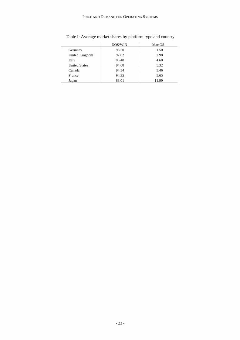
The DOS/WIN platform reaches a 95% market share on average as shown in Table I. The

market share of the DOS/WIN platform has a relatively larger variance and falls in a range between

1.5% for Germany and 12% for Japan.

[Place Table I about here]

Features of the home segment14

All together our database on the home PC market contains 23701 observations. In addition to

the number of countries and period, this large size is explained by the number of vendors per country.


- 5 -

Considering each country separately, seventeen firms on average have an annual market share larger

than one percent for at least one year over the period 1995-1999.

Behind the curtain, the picture is different. The industry comprises “local” firms sometimes

quite large in a single country but often quite small worldwide. Often multinational firms have

relatively small market shares outside their home countries. From inspecting the data, several facts can

be noticed. Only seven vendors exceed the one-percent market share threshold in each of the five

years over the period 1995-1999. Only four firms present in the seven countries meet the same criteria.

Hence the industry is not concentrated.

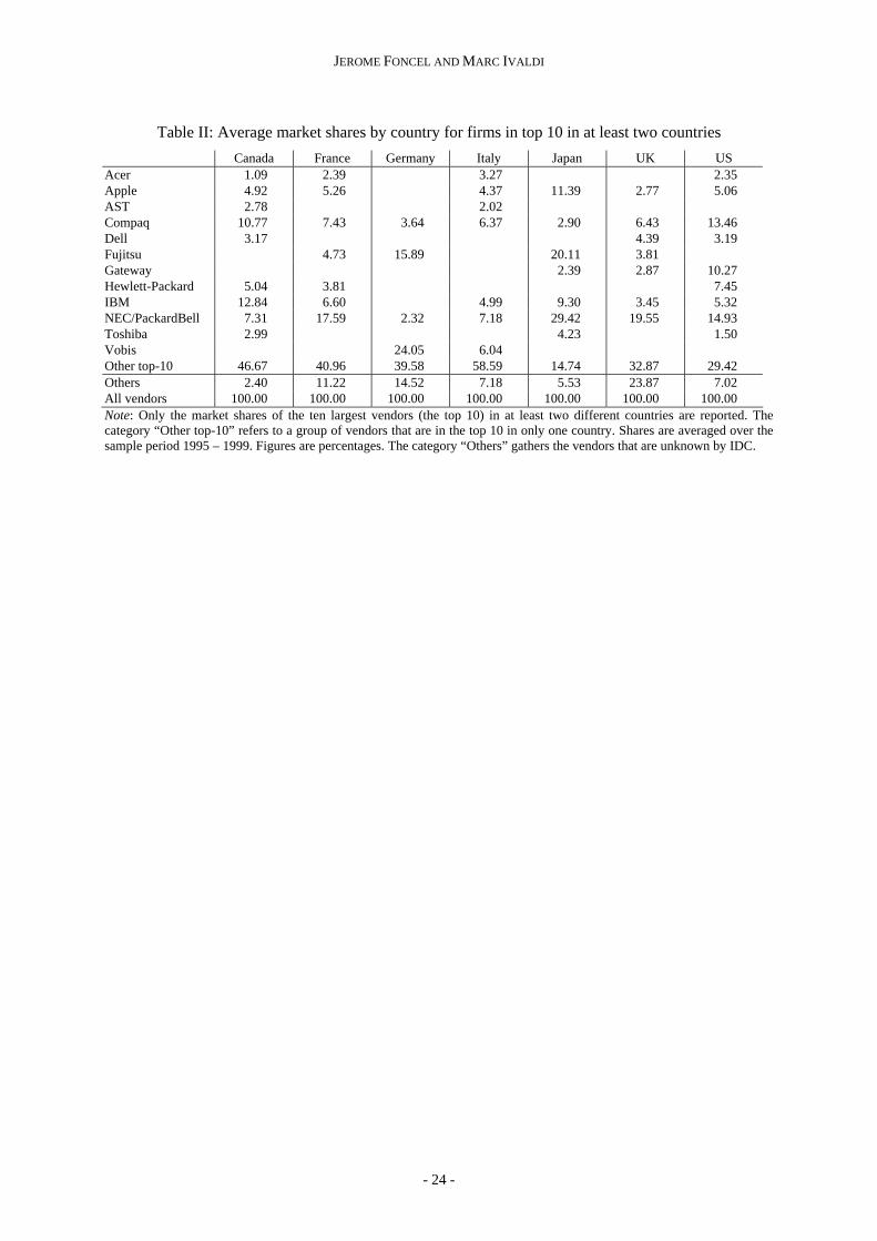
The ten largest vendors (the first ten vendors ranked by decreasing market shares, i.e., the top

10) in at least two countries over the period 1995-1999 are provided in Table II. Note that this list

differs from one country to another. In each country there are “national champions” that are not

present in the other countries. Note the large market share reached the category “Other top 10” that

includes all vendors that are in the top 10 in only one country.15 In addition, Table III displays the G7

shipments and market shares for the ten largest firms in each year. Note that the ranking evolves

significantly over time and so the volatility of market shares across PC brands. Given these facts, we

may draw two conjectures. First, competition in the home PC segment that is growing fiercer over the

period; second this market segment exhibits significant idiosyncrasies among countries.

[Place Table II about here]

[Place Table III about here]

[Place Table IV about here]

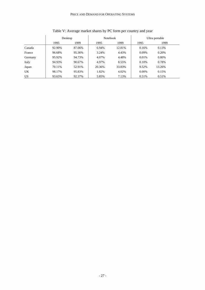
Differentiation is not an empty word in this industry. First, the number of brands present in the

home PC market of a country in a given year is quite large, with an overall mean of 79 brands per

country and year. According to Table IV, the number of brands, which is correlated with the

population size, is slightly increasing over time for most countries. Second, PCs differ in their form,

the so-called factor form. For the home segment, three form factors are usually identified: desktop,

laptop or notebook, and ultra portable. Table V shows that the share of notebooks and ultra portables

increases over time and it is much larger in Japan than in any other country.

The speed of processors could be an additional candidate of market differentiation. Over the

period 1995-1999 different generations of Intel-compatible processors appeared and disappeared.

Basically each year a new processor with an increased speed becomes available. Now, as the length of

life of each Intel processor generation is around three years and since the old generation disappears

from the market as soon as a new one arrives, most PC brands shipped to different destinations in a

given year can be equipped with five different leading types of Intel processors.16 As far as the MacOS

platform is concerned, the IDC database allows us to distinguish three types of Motorola processors:


- 6 -

68030 and below, the 68040 (at a 25 - 33 MHz speed) and the PowerPC.17 Clearly this dimension of

differentiation in terms of processor type would be meaningful in an intertemporal approach.

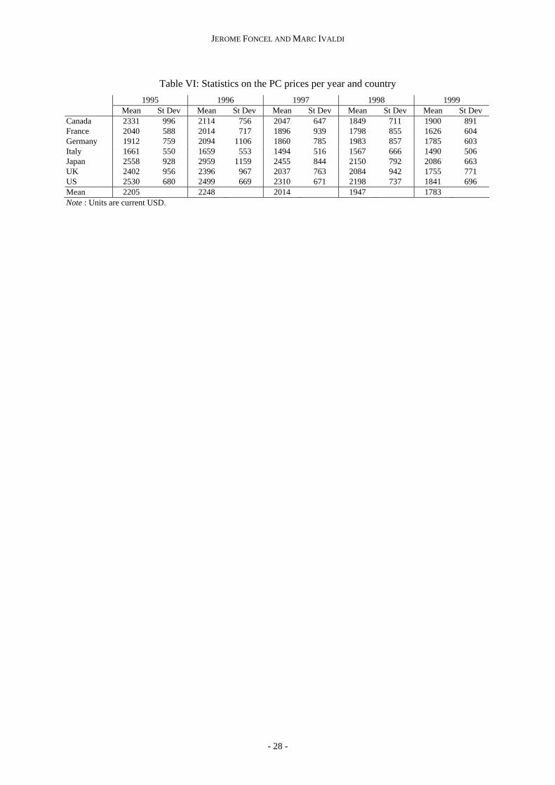
Finally, the database also provides prices of the different brands. IDC computes for each brand

an “Average Selling Price” which is “the average end-user (street) paid for a typical system configured

with chassis, motherboard, memory, storage, video display, and any other components that are part of

an “average” configuration for the specific model, vendor, channel and segment.” According to Table

VI, the temporal pattern of annual average prices for each country exhibits a decreasing trend. Note

that these average prices are not controlled for the differences in the technical characteristics of PCs

shipped in the different countries. The overall mean is equal to 2205 in 1995 and it is only 1783 in

1999. In addition the standard deviations of the price distribution in each year and in each country

show a large price variability. Again these facts support the view that competition is getting fiercer

over time.

[Place Table V about here]

[Place Table VI about here]

III. THEORETICAL MODEL

The key features of the data are the price volatility and the degree of product differentiation

and variety. Fully recognizing this fact, the model below allows us to characterize supply and demand

side effects in order to explain price differences and the behavior of vendors. This model has two main

components: a demand system, which is based on the nested logit model, and a supply system derived

from a Nash equilibrium.

Demand system

There are M separated markets, each market 1,....,m M= being defined as a country at one

period. Let mN be the potential market size corresponding to the total number of potential consumers.

In much of what follows, we drop the index m for simplicity.

Each consumer 1,...,n N= can buy one and only one computer in one market, or each can buy

an “outside good”. That outside good could be a substitute to the use of a new computer, like a

computer already in use at the consumer home, a handheld computer, or a network computer, or it

could be to buy no computer at all.

Given our data, three choices seem relevant: form factor, client operating system, and brand.18

We assume that they are arranged in the following order. In the first stage of choosing a computer, the

consumer selects one of the three PC form factors or the outside good O. There are three possible form


- 7 -

factors: desktop D, laptop L and ultra portable U. Let g be the choice made by the consumer in the

choice set { }OULDG ,,,= . In a second stage, the consumer chooses between two client operating

systems, namely DOS/WIN and MacOS. Let h be the operating system selected by the consumer in

the set gH of operating systems available conditional on the choice g in the first stage. In our case,

both operating systems are available for all three form factors, so the two operating systems are always

available, i.e., { },gH WIN MAC= for any g. Finally, in the third stage the consumer chooses one

brand k in the set ghK of PCs available conditional on the choice ( ),h g .

This sequence of choices corresponds to a natural order in the sense that the hardware form is

selected before the software. An alternative sequence consists of inverting the first two decisions by

choosing first the operating system, then the PC form, and finally the PC brand. This order would be

more realistic when the customer is aware of the working of a PC product and its environment. Which

sequence of choice is relevant is left as an empirical issue.

The indirect utility level achieved by consumer n from the choice of brand k using the

operating system h installed on a specific form g is given by

(1) n n

khg khg khg khg khgU V pα ξ ξ ε= − + + + , where khgV is a deterministic part that depends on the specific brand, operating system and form factor

chosen by the consumer, ξ is a market specific component, khgξ is a random term reflecting the effect

of unobserved characteristics of brands on the mean utility, khgp is the price of the selected product,

α is the marginal utility of income and is a parameter of interest to be estimated and nkhgε defines the

unobserved variables that explain the departure of consumer n’s behavior from the common utility

level. The random term nkhgε is specified as a weighted sum of unobserved variables as follows

(2) ( ) ( )1 1 , 1,...,n n n n

khg g H hg K khg n Nε ν σ ν σ ν= + − + − ∀ = where Hσ and Kσ are parameters to be estimated. The random components are assumed to be

distributed in such a way that they give rise to the nested logit model. (See Ben-Akiva and Lerman

[1985] or McFadden [1981] for details.) In the sequel, we drop the indices h and g when there is no

confusion.

This model allows us to decompose ks , the unconditional probability of selecting a PC k, as

the product of three conditional probabilities: i) ( ),s k h g , the probability of choosing brand k

conditional on the form factor g and operating system h ; ii) ( )s h g , the probability of choosing the

operating system h conditional on form factor g ; iii) and ( )s g , the probability of choosing PC form


- 8 -

g. Recall two important features of this nested logit model. First the higher Kσ , the higher the

correlation between products of the same sub-group, i.e., the same client operating system, and the

higher Hσ , the higher the correlation between products of the same group, i.e., the same form factor.

Second, the parameters must satisfy 1 0K Hσ σ≥ ≥ ≥ for the model to be consistent with stochastic

utility maximization.

Finally, aggregating these probabilities over all consumers generates market shares. Using

simple algebra and some normalizations, ks , the share of product k in a market, can be written in

logarithmic form as

(3) ( ) ( ) 0ln ln , ln lnk k k K H ks V p s k h g s h g sα σ σ ξ ξ= − + + + + + , where now ( ),s k h g designates the share within the nest defined by form factor g and operating

system h, ( )s h g is the share of the operating system within the nest defined by form factor g, and 0s

is the probability of choosing the outside good.19

The different shares are measured as

(4) ( )

( )

,

, ,

,hg

g hg

k k

k hg k kk K

hg g hg kh H k K

s q N

s k h g q Q q q

s h g Q Q Q q

∈

∈ ∈

=

= =

= =

∑

∑ ∑

where hgQ is the total quantity of products belonging to the nest ( ),h g shipped by all firms present on

the market, and gQ is the total quantity of products belonging to the nest g . These variables are used

for deriving the expressions of elasticities, i.e., own-price elasticity, cross-price elasticity within the

same group g and the same sub-group h, cross-price elasticity within the same group g and between

different sub-groups h and cross-price elasticity between different groups g.20

Supply system and equilibrium

Consider a vendor f. Let fS be the set of PCs that firm f offers on one market. The vendor

chooses the set of prices for maximizing profits, i.e.,

(5)

{ }( )

,Max

f fk

k k kp k S k S

p c q∈ ∈

−∑ ,

where kc , the marginal cost of producing brand k, is constant.21,22 Assume Nash-Bertrand competition

for the home PC industry in each separate market and consider demand functions as specified in the

preceding section. The markup kπ , for each product k belonging to the nest ( ),h g , is given by23


- 9 -

(6) ( ){ } { }

1

0' '

1 11

g g

f fh g hgf

k k hg hg g hg hg kh H h g G g h HK h g hg

Q Qp mc r Q r r π

α σ′

−

′ ′

∈ − ∈ − ∈′ ′

⎡ ⎤− = − − Γ − Λ ≡⎢ ⎥

− Γ Λ⎢ ⎥⎣ ⎦∑ ∑ ∑ ,

where

fhg

fhg j

j K S

Q q∈ ∩

= ∑ is the total quantity of products belonging to the nest ( ),h g shipped by firm f

and

(7)

( ) ( ) ( ){ }

0

0 0'

1 1 1 1 1 1 1 1, , ,1 1 1 1

1 1, .1 1

g

H Hhg g

K H hg H g H g

fh gf f

hg hg g hg hg hg hg g hgh H hK K h g

r r rQ Q N Q N N

QQ r r r r Q r r

σ σσ σ σ σ

σ σ′

∈ − ′

⎧ ⎛ ⎞= − + + = + =⎪ ⎜ ⎟− − − −⎝ ⎠⎪

⎨⎡ ⎤⎪Γ = + − Λ = + − + − Γ⎢ ⎥⎪ − − Γ⎣ ⎦⎩

∑

The existence of a solution to the set of Equation (7) for all products of each vendor present on

the market is based on results derived by Caplin and Nalebuff [1991] and by Anderson, De Palma and

Thisse [1992]. Note that Equations (6)-(7) show that the markups take values on a restricted set.

Indeed they are only determined by only three parameters of interest , ,K Hα σ σ , and by the aggregate

quantities associated with the nests of upper levels of the decision tree. In other words, the number of

nests plays a crucial role in the continuity of the function defining the markups.

IV. SPECIFICATION ISSUES

The demand Equation (3) and the pricing Equation (6) form a simultaneous equation system in

the sense that prices and quantities are jointly determined. This system is estimated by applying the

nonlinear three-stage least-squares estimator, once some additional elements of specification are

settled. They concern the final parameterization of the demand and pricing equations, the marginal

utility of income, the choice of market size, the estimation method and the selection of instruments.

Final parameterization of the demand and pricing equations

The deterministic part of the indirect utility for each product is specified as a linear

combination of available exogenous variables, among which a specific effect of the firm that produce

this brand and dummy variables for the type of OS, PC form factor, and processor that characterizes

this particular brand. The market-specific variable ξ in Equation (3) is specified as a set of dummy

variables referring to countries and time periods, also allowing for cross effects between countries and

firms and between countries and OS. Let x be the set of all these variables. The precise elements of

this vector are provided below together with the estimation results.


- 10 -

Using the market index m and the notations introduced so far, the demand equation is now

stated as

(8)

, ,

ln ln ln

hg

hgmkm kmkm m km K H km

m km hgm gmk K h g

Qq qx pN q Q Q

β α σ σ ξ

∈ ∀

= − + + +− ∑

,

where β is a vector of parameters to be estimated. Note that the parameter α is supposed to be

country specific.

Concerning the pricing equation, we specify the marginal cost as

(9) ( )expkm km kmc x γ ζ= + , where γ is a vector of parameters to be estimated and ζ is a random term that stands for the

unobserved component of the marginal cost. Based on Equation (9), the pricing equation becomes

(10) ( )ln km km km kmp xπ γ ζ− = +

At this point, note that the pricing equation can be viewed as a hedonic price equation that satisfies

behavioral and structural constraints through the markup. In other words, it shows that just considering

a standard hedonic price equation for analyzing the pricing behavior in this differentiated-products

market would certainly cause a misspecification.

Specification of the marginal utility of income

The marginal utility of income α is assumed to vary across countries. More specifically, this

parameter is made function of the Gross National Product per capita (in current USD), in each country

in each year, according to:

(11) 0 1m mGNPα α α= + ,

where 0α and 1α are parameters to be estimated. In addition to providing a more flexible model, this

specification introduces a wealth effect. If GNP per capita is a proxy for wealth, one should expect 1α

to be negative. Richer countries might be expected to be less sensitive to PC prices. Note that, by

specifying the parameter α as in Equation (11), we introduce a trend in the model through GNP.


- 11 -

Choice of the market size

While not stressed in the literature, the choice of the market size plays an important role in the

measurement of elasticities, and in particular the measurement of the aggregate elasticity for PCs. To

see that, note that the aggregate elasticity depends in part on the amount of utility received from all the

“inside” goods relatively to the utility level provided by the sole outside good. From Equation (8), we

can define the gross utility level, i.e., km km kmxδ β ξ= + , as

ln ln ln hgmkm kmkm m km K H

m k m hgm gmk

Qq qpN q Q Q

δ α σ σ′

′

= + − −−∑

.

If the structural parameters α and σ s do not vary much, the gross utility level provided by each PC

decreases as the market size gets larger. The outside alternative becomes more attractive and the

aggregate elasticity increases. So changing the market size is changing the value of the outside

alternative and the level of the aggregate elasticity.24 It is then a crucial task to determine the potential

market size mN , i.e., the potential number of consumers in each country, and to test how it affects the

estimates.

A standard measure used by several studies in the literature is the number of households. One

may question the relevance of this measure. Since a PC is an object of individual usage (particularly

when we consider laptops), one might admit that the size of the population is more appropriate for the

home PC segment than for the automobile market for instance.

An admissible range for the market size is easily defined. Clearly, on one side, the population

is an excellent candidate for an upper bound of the potential market size. Indeed, some individuals are

not able to buy PCs, like babies for instance; some others have bought a PC equipment recently and

are not considering renewing it. On the other side, a lower bound for this market size is obviously the

total amount of PC shipments to the home segment, which would imply that no consumers choose the

outside good.

Since the right potential market size (in the range defined by the population size and the total

volume of shipments) is not known, we propose to select several values in this range in order to check

for the robustness of our results. We proceed as follows. Given the two identified bounds of the range

of values; the market size could be either proportional to the population size or to the total amount of

PC shipments to the home segment. We adopt the second option and we set the total number of

potential consumers as the average annual shipments of PCs in a country multiplied by a number τ

that we call the market size factor. The motive for our choice is simple. The population size does not

change much year by year and so, is not able to account for the rapid diffusion and attractiveness of

PCs in the population. Note that a log-log relation between the number of households and the total

quantity of PCs shipped in a year (with or without constant) provides a R² equal to 99%. As the total


- 12 -

quantity of PCs shipped in a year is able to reflect the dynamics in this industry, it is an excellent

candidate to calibrate the market size here.

It remains to select values for the market size factor. Admissible values are all strictly greater

than one. The value one corresponding to the lower bound cannot be used because of the logarithmic

form of the demand equation given by Equation (8). In effect a value of τ slightly greater than 100

provides a market size that is roughly equal to the population size on average.

In practice, the measure of market size is obtained as follows. First, for each country and each

year, we compute average quarterly total shipments. Second, we inflate this number by the market size

factor τ taking values in the range [2,100]. This method permits us to obtain a potential market size

that is country-specific and annually modified. Allowing the market size to change over time provides

us with more flexibility.

Estimation method and choice of instruments

Summing up, in the system formed by Equations (8) and (10), the parameters to be estimated

are the β s, the γ s, the α s, Kσ and Hσ . Note that a subset of parameters including the β s and 0α ,

1α , Kσ and Hσ , could be estimated directly from the demand equation without the need of the

pricing equation. However, estimating the two equations together improves the quality of estimates.

This system of Equations (8) and (10) contains several endogenous variables: price, shipment

quantity, and shares of different nests in the decision tree. Following the usual practice, the

characteristics of PCs are assumed to be exogenous, an assumption that allows us to identify the

model. In a long run perspective, it would be a too strong assumption, as the choice of computer

characteristics by firms might result from a strategic behavior in a dynamic setting. Here, considering

a short run horizon and recognizing that the sole characteristic we observe is the processor speed, it is

fairly reasonable to assume that the level of technical progress on processors is a state variable for PC

vendors.

A further aspect of this econometric model is that the error terms ξ and ζ may be correlated.

In these conditions the nonlinear three-stage least-squares estimator is an adequate choice given the

structure of the econometric model. This method requires choosing a set of instrumental variables.

Given the variables available in our data set, there are not too many alternatives. The set of

instruments chosen here contains all exogenous variables that enter the model and some functions of

the variables linked to the characteristics of the home PC segment. For each country and time period,

one defines, for a given brand, the following instruments: the total number of brands, the number of

brands per vendor, the number of brands per form factor, the number of brands per operating system,

the number of brands per type and speed of processor, the number of brands that a vendor sold with

the same PC form factor, the number of brands that a vendor sold with the same operating system, and

the number of brands that all the competitors of a vendor sold with the same form factor. This set of


- 13 -

variables has been selected after trying different combinations of variables. This choice is in the line of

a tradition initiated by Berry, Levinshon and Pakes (1995).

V. EMPIRICAL RESULTS

Parameter estimates

Table VII presents the sets of estimated parameters of interest, corresponding to the different

values for the market size Kσ and Hσ discussed above. Clearly these estimated values are stable from

one experiment to the other. However, note that, as market size increases, 0α decreases, 1α increases,

and the combined effect is that the marginal utility for money mα slightly decreases. The intra-group

correlations Kσ and Hσ (i.e., PCs sharing the same OS and the same form factor and PCs sharing the

same form factor) also decrease.

Several other remarks about Table VII are in order. First, all parameter estimates are

significantly different from zero in all experiments. Note that, as Kσ and Hσ are different from zero,

the simple logit model is therefore rejected by the data. This means in particular that the home

segment involves several levels of competition, across PC brands, across operating systems and across

PC form factors. In other words, differentiation matters along these two dimensions, i.e., OS and PC

form. Second as expected, 0α is positive and 1α is negative. By using the GNP per capita as a way to

introduce country-dependent effects of PC prices on demand, we have identified a wealth effect.

Third, these effects of price on demand are always negative for all countries, because mα defined by

Equation (11) is always positive. Fourth, the parameter Kσ is greater than Hσ , which is required for

the model to be consistent with utility maximization.25

[Place Table VII about here]

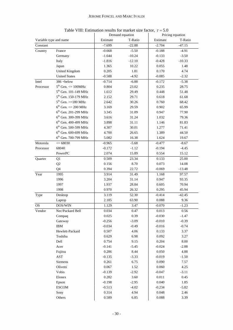
Table VIII presents the other parameter estimates for 5.0τ = .26 Most of these are coefficients

for dummy variables; that they tend to differ significantly from zero implies that substantial

differences in demand and cost exist across countries, form factors, and so forth. The general pattern

of the estimates seems sensible. First, for example, both consumer utility and marginal cost rise with

increases in the processor speed (for both Intel-compatible and Motorola/PowerPC processors).

Second, everything being equal, the higher value in term of utility associated with the desktop dummy

compared to the laptop or small portable dummies picks up an un-modeled distribution of tastes in the

population over the ‘portability versus price’ combinations.27 Third, as expected, a desktop has a lower

marginal cost. Fourth, while the type of client operating system has no significant effect on marginal


- 14 -

cost of PCs, DOS/WIN provides a net utility gain. Note that one could interpret this parameter

associated with the type of platform as a measure of the individual valuation of a membership to the

DOS/WIN network.

As far as the time variable is concerned, note that the quarterly effect seems realistic. Demand

is higher in winter probably due to the Christmas period; costs are lower in winter because one could

expect that more low-end machines are sold for Christmas. With respect to the annual effect, marginal

costs are decreasing over time, which could indicate that we have identified an effect of technical

progress on production costs, while the decreasing time effect of year on utility levels could be

interpreted as an effect of satiation of demand. This last statement merits further comments.

We conjecture that the combination of the time and country dummies is a proxy for the effect

of the installed base of PCs in each country. A coherent series for the equipment rate can be

downloaded from the World Bank web site. This equipment rate in PCs, which measures the

importance of the installed base, appears to be strongly trended, with the trend being country specific.

Then the decreasing time effect of year on utility levels could be due to a decreasing direct network

effect of the installed base. Note however that, given that we do not take into account in our model

how the installed base is in turn affected by the supply and pricing decisions of firms, the model is not

able to identify the effect of such network effects. This is an open issue.

[Place Table VIII about here]

Concerning the country and firm effects, they are not straightforwardly interpretable. Note

however the significant presence of a specific dummy variable, named “Others,” that stands for an ad

hoc aggregation of small firms not individually identified in the data. Finally cross effects between

countries and vendors often differ from zero, a sensible result. Adding further cross effects (in

particular country-time fixed effects) either does not significantly improve the goodness-of-fit of the

model or leads to convergence problems.

Last, we provide the first stage R-squared associated with each parameter as a ‘measure of

quality’ for the instruments used at the estimation stage. These values determine the acceptability of

the selected instruments in measuring the fraction of the variation of the derivative of the objective

function associated with the parameter that remains after projection through the instruments. Ideally,

the R-squared-should be close to 1 for exogenous derivatives. In our case, the R-squared values are

exactly equal 1 for each parameter associated with an exogenous variable. For the parameters of

interest 0α , 1α , Kσ and Hσ , the R-squared values are 0.54, 0.68, 0.42 and 0.83, respectively. These

values are large enough to reflect a good choice of instruments for the endogenous variables.


- 15 -

Elasticities and markups at the brand and firm levels

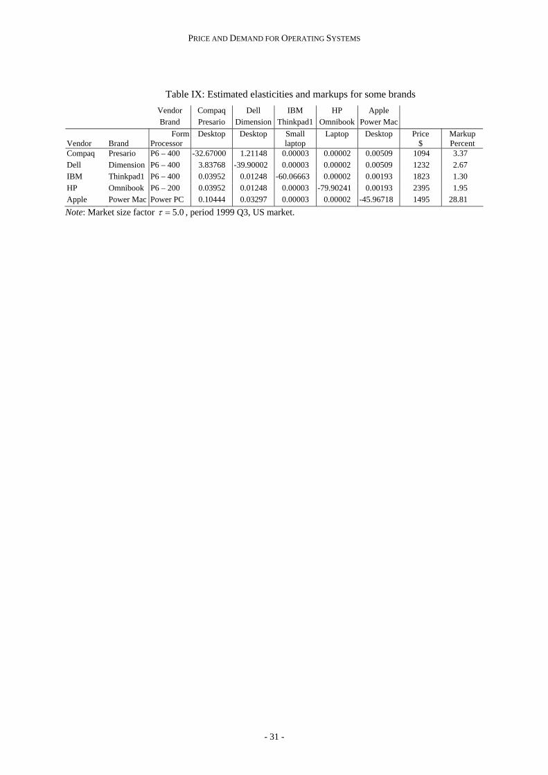
Estimated own- and cross-price elasticities as well as markups for some particular brands are

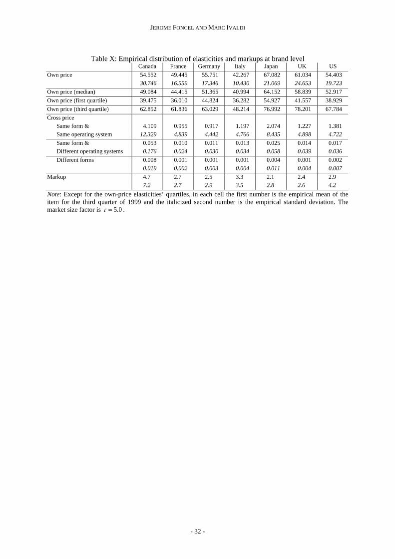
presented in Table IX, and some statistics on the overall distribution of these estimated elasticities and

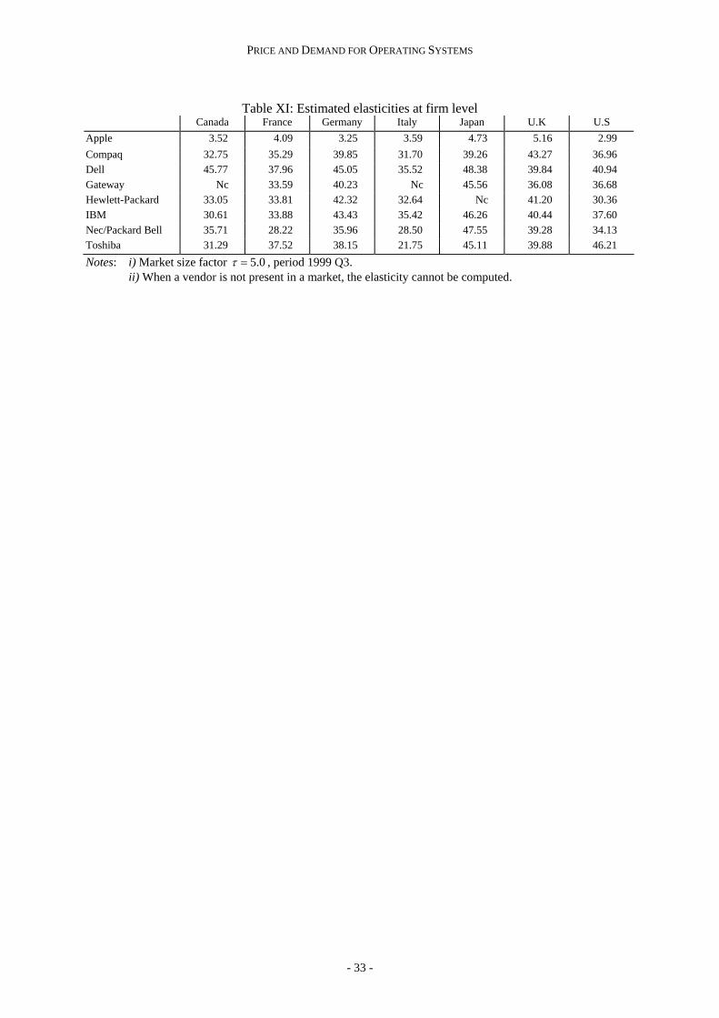
markups at the brand level are provided in Table X. Table XI presents the estimated values of

aggregate elasticities at the firm level, for some of the major vendors. These latter elasticities are

calculated as the percent change in shipments of all products sold by a firm when the prices of all

these products are increased by one percent.

[Place Table IX about here]

[Place Table X about here]

[Place Table XI about here]

Before discussing these elasticities and markups, it is useful to return to Table VII and to

assess the values taken by the parameters of interest, in particular Kσ and Hσ . Indeed, these

parameters play a crucial role in the formulas of the different types of elasticity. (See the Journal’s

editorial Web site which provides the formulas of elasticities in Appendix C of our supplemental

document.) First, because Kσ is significant and close to (although statistically different from) one, PC

brands are close substitutes, which is a realistic result. It means that individual preferences are

correlated across PCs within the same group defined by the type of operating system and that one may

expect fierce competition between PCs belonging to the same platform type. It is exactly what the

estimated values of elasticities tell us, in particular when one looks at the cross elasticities among

products sharing the same form and the same OS. (See in particular the second row of Table X or the

cross elasticity between the Compaq Presario and the Dell Dimension in Table IX.) Second, because

Hσ is significantly different from zero and is not close to Kσ , preferences are correlated across PCs

of different platforms, but this correlation is much weaker than across PCs within a platform. This fact

is reflected in the values taken by the estimated cross elasticities displayed in Table X.

Two main remarks can be made on the estimates of elasticities and markups. First, the own-

price elasticities at the brand level for all types of PCs (whether they are run under DOS/WIN or

MacOS) are high. (See Table IX.) One could blame the nested-logit model for these results, because,

as we explain above, the flexibility of this model to represent preferences is limited. However these

results are not counterintuitive. Indeed, as a PC is a durable good for a household, i.e., a commodity

that is bought once for a “long period”, any price change on a brand at a given time could have a

strong and rapid effect on the sales of this brand, particularly when plenty of substitutes are present on

the shelves of distributors. Moreover, the quartile ranges for the own-price elasticities reported on

Table X show that the median is systematically lower than the mean and the distributions appear to be

more concentrated on low values. So our model is able to account for large variances and asymmetric


- 16 -

patterns. Second, we observe that the price elasticities at the firm level are quite high for all PCs based

on the DOS/WIN platform and are much smaller (higher) for PCs based on the MacOS platform. (See

Table XI.) The corollary of this result is that any DOS/WIN PC has a rather small markup while any

MacOS PC has a very high markup. (See Table IX again.) This result indicates that the home segment

of the PC manufacturing industry is highly competitive. Now, the fact that we observe simultaneously

high own price elasticities at the brand level and high markups for MacOS products must be related to

the structure of the decision tree in our model. On one branch, we have a lot of firms in competition,

on the other branch there is basically one firm producing all the brands. Our nested-logit model is not

flexible enough to smooth this situation and probably amplifies the phenomena.28

Aggregate elasticity of PCs

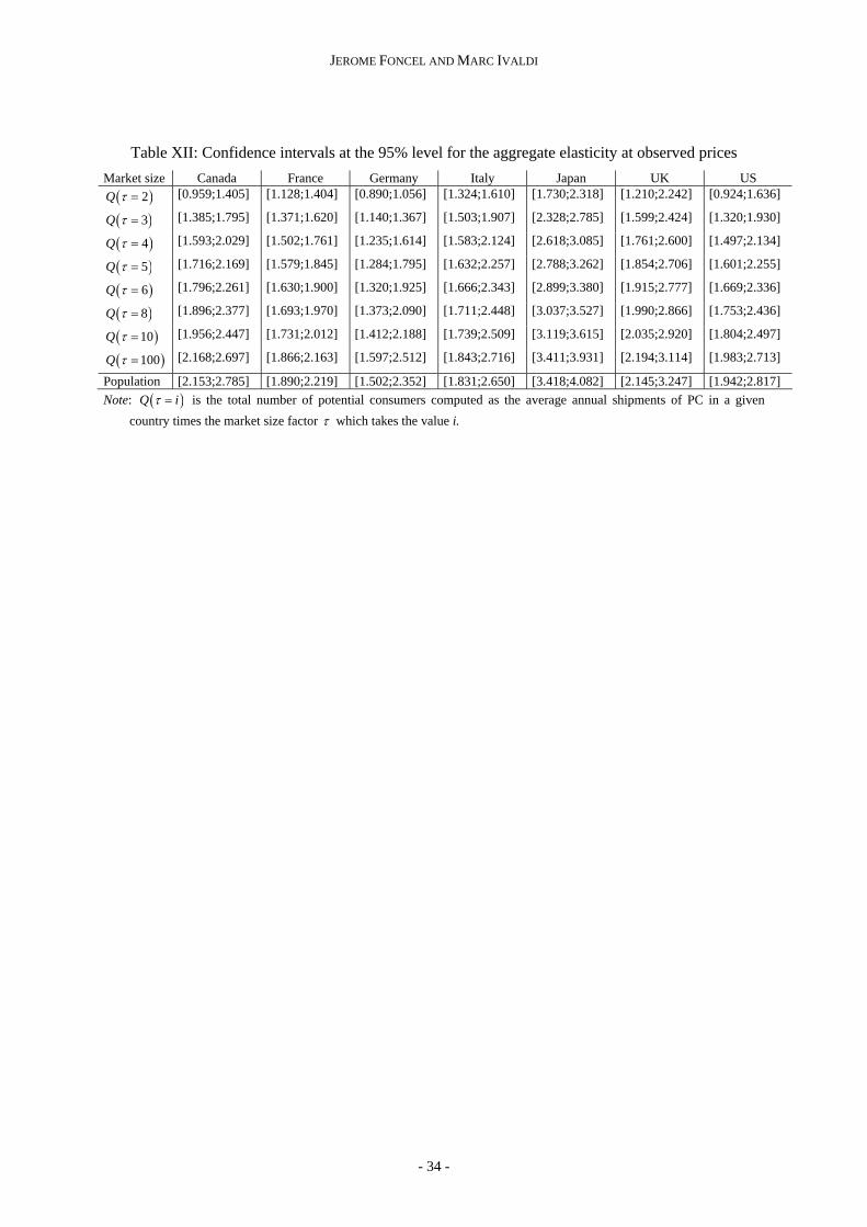
Table XII provides our estimates of the elasticity of aggregate demand of household PCs, for

all the G7 countries for the third quarter of 1999 and for different values of market size. The aggregate

elasticity is calculated as the percentage change in total shipment due to a one-percent increase in the

price of all products on the market. For each country m at each period t, the aggregate elasticity tme is

defined according to

(12) ( )

0

1

logtm

j tmj A

tm tm tm tm

s pe p p s

λ

λα

λ∈

=

⎡ ⎤∂ ⎢ ⎥

⎣ ⎦= = −∂

∑,

where tmA is the set of all products sold at period t in country m, js is the share of computer j (See the

Journal’s editorial Web site for a presentation of the demand system in Appendix B of our

supplemental document), tmp is the vector of observed prices and p is the share weighted average

price for the outside good. (See Werden [1997].) This formula shows that the aggregate elasticity

would be affected by the choice of market size through the market share of the outside good.

Confidence intervals for the estimates of this aggregate elasticity can then be computed by applying

the delta method to the function tmf defined by Equation (12).

[Place Table XII about here]

First, note that our estimates of the aggregate demand elasticity for the third quarter 1999 are

highly sensitive to the choice of market size. The elasticity corresponding to the upper bound of

experiments (when market size is equal to the population size) is 1.5 to 2 times the value

corresponding to the lower bound ( 2τ = ). Second, these elasticities are very precisely estimated as


- 17 -

the mean standard error over countries and market sizes, equal to 0.149, is small compared to the mean

values. For instance, the mean elasticity over countries at the market factor 5=τ is 2.05, with the

lowest value being taken by Germany, namely 1.53, and the highest value by Japan, i.e., 3.02. (These

values are mid points of the corresponding confidence intervals.) Given that the demand of OS is a

derived demand, these numbers are fairly reasonable and realistic.

We may also compute estimates of the aggregate demand elasticity when only PCs based on

the DOS/WIN platform are considered, i.e., when prices of all such computers rise by 1 percent while

the prices of Macintosh and other computers remains unchanged. The elasticities for DOS/WIN PCs

alone are in general slightly higher, with 1.99 for the U.S and 3.13 for Japan. These results – a

complete set is available from the authors - are to be compared to their counterparts for the whole

market, i.e., 1.93 for the U.S and 3.02 for Japan.

VI. COUNTERFACTUALS

The estimated model of the home PC segment allow us to estimate the price elasticity of

operating systems and to derive implications for the price of such software. We focus our attention on

the price of DOS/WIN systems. One limitation of our approach is that our analysis of the monopoly

price of Windows is based only on the home segment. To our knowledge, Microsoft cannot readily

price discriminate between copies of Windows installed on PCs used for the home segment and other

segments. As a result, if the price elasticity of demand for the home segment is larger than the

aggregate price elasticity of demand across all segments, we are likely to understate the monopoly

price of Windows.

In computing the profit maximizing price of Windows below, we assume that Microsoft

proposes a unique linear price. However, it is known that Microsoft offers discounts to the major

OEMs (which accounts for not more than 60% of the market all together) and not to all PC

producers.29 We have no information on these contracts and we are just able to construct an average

price paid by OEMs for licensing Windows 95 or 98. Empirical evidence on the effects of nonlinear

prices on the measure of market power has not received a considerable attention in the literature based

on structural econometrics. (See however Ivaldi and Martimort, 1994, Brenkers and Verboven, 2002,

Miravete and Röller, 2003, Villas-Boas, 2003.) It is a complex question. One main difficulty is that

non linear price schemes are not exogenous and must be determined at the equilibrium together with

the parameters that characterize demand and supply. Note however that our approach is compatible

with two-part tariffs. In effect, in our model, the fixed part of any two-part tariff cannot be separated

out from the marginal cost, which would be required to obtain the profit-maximizing two-part tariffs.

As price schedules are not observed, this identification problem cannot be solved.


- 18 -

The Nash monopoly price

Consider the situation where the seller of DOS/WIN maximizes its profit assuming that buyers

of DOS/WIN, who are sellers of PCs, choose their best strategy in prices. The equilibrium price in this

case is called the Nash monopoly price of DOS/WIN.30 Let WC be the set of products equipped with

the operating system DOS/WIN and AC be the set of products equipped with the operating system

MacOS. The model provides the demand for personal computer k,

(13) ( ), ,w A w Ak kq q p p k C C= ∀ ∈ ∪ ,

where wp is the price vector of PCs equipped with DOS/WIN and Ap is the price vector of PCs

equipped with MacOS. Define wkp as the prices of the PC k powered with an Intel processor but

without the operating system installed, and wp as the price of DOS/WIN. Then

(14) w wk k wp p p= − ,

for some base levels of prices for PC k, wkp , and for DOS/WIN. As already discussed, the price wp is

assumed to be constant across computer vendors. Now the demand of DOS/WIN is obtained as

(15)

ww k

k C

q q∈

= ∑ ,

and the price elasticity is

(16) w w w

W k w k ww

k C k C k Cw w k w

q p q pp q p q

ε′ ′∈ ∈ ∈

⎛ ⎞ ⎛ ⎞∂ ∂≡ =⎜ ⎟ ⎜ ⎟∂ ∂⎝ ⎠ ⎝ ⎠∑ ∑ ∑ .

The second part of this last equation is obtained by applying the implicit function theorem. An

increase in the price of operating systems causes a decrease in the demand for product k through the

rise of the price of product k, everything being equal. However it also increases the prices of

competing brands, which push up the demand for product k. The result of this process is not trivial.

When the seller of the client operating system DOS/WIN is maximizing its profit taking the

non-OS component of the prices of PCs ( wkp ) as given, it must choose the price wp∗ that satisfies

(17)

1

w ww w

ww w k w

wk C k Cw k wp p

p c q pp p q∗ ∗

−∗

∗′ ′∈ ∈

⎡ ⎤⎛ ⎞− ∂⎢ ⎥⎜ ⎟= −⎜ ⎟∂⎢ ⎥⎝ ⎠⎣ ⎦∑ ∑ ,


- 19 -

where wc is the marginal cost of producing DOS/WIN. This price corresponds to the monopoly price,

assuming that vendors are selecting their best strategy.

The basic program of an OEM is given by Equation (5) where the consumer price kp is

decomposed into *w

wk pp + . The OEM chooses w

kp for each product k while taking the optimal strategy

*wp of Microsoft as given. The first order condition associated with product k is given by Equation (6)

in which we replace the observed values of gQ , hgQ and fhgQ by their theoretical counterparts in terms

of logit probabilities. The system formed by Equation (17) and by the transformed Equation (6) must

be solved numerically at the estimated values of the parameters. In the simulation experiments below,

we assume that the marginal cost of producing DOS/WIN is zero. In this case, Equation (17) just tells

us that, for maximizing profit, the optimal decision is to price at the point where the aggregate

elasticity of demand is unity.

Table XIII gathers the confidence intervals for the simulated Nash monopoly prices that we

obtain for the G7 countries in the third quarter of 1999 and for the different market sizes. These

confidence intervals are computed by using the delta method again.31 First, wholesale prices of PCs

increase. Given the small margins we find for DOS/WIN PCs, it is not surprising that these increases

are roughly in the order of magnitude of the increase in the price of DOS/WIN. That is to say, the

pass-through is here almost complete, indicating that OEMs do not have a strong countervailing

power. Second, all monopoly prices are precisely predicted. For instance the largest value for the

standard errors is $22.42 for the U.S when the market size factor is 2=τ . Third, the smallest lower

bound of our confidence interval is $497 while the largest upper bound is $698. The range is mainly

affected by the choice of market size. Indeed, as expected, the larger the potential market size, the

larger the monopoly price even if the OS prices are less sensitive to the choice of market size than the

aggregate elasticities. Finally, the Nash monopoly prices take values that are roughly ten times the

actual price of DOS/WIN (around $ 50-60), and three times the sum of the actual DOS/WIN price and

the average price of the basic Microsoft’s DOS/WIN applications (like Word, Excel, Powerpoint) that

Microsoft can expect to sell as complements to the operating system and are evaluated to cost around

$200 all together.32

[Place Table XIII about here]

To assess the robustness of our findings, an anonymous referee suggested that we perform an

experiment consisting in dropping all PCs with prices larger than $5,000, which represent 0.83% of

the whole sample. Indeed we do not want high price outliers to help identify the marginal utility for

income and the correlation parameters which controls the substitution patterns for all computers. We

re-estimate the model for 5=τ and find 332.160 =α , 264.01 =α , 941.0=Kσ and 361.0=Hσ . Note


- 20 -

that the sign of 1α is now counterintuitive although the marginal utility of income remains positive as

expected. We remark also a slight decrease of 0α and an large increase of Hσ . With these new

estimates, the aggregate elasticity becomes 1.82 and the monopoly price is now $575, in the case of

the U.S. in the third quarter of 1999. Recall that these values are 1.93 and $568 respectively when we

use the whole sample. For other countries and/or other periods, elasticities and simulated monopoly

prices do not vary much either.

Our estimated profit-maximizing prices of Windows are below the estimate of $900, provided

by Reddy, Evans and Nichols [1999] in the context of a model of perfectly competitive PC suppliers.

Werden [2001a] explains the high estimate found by Reddy et al. as a direct result of the unrealistic

assumption of homogeneity of PCs made by these authors. He shows that, in a model with

heterogeneous products but independent demands, the present price of Windows turns out to be the

profit-maximizing price when one considers plausible values for the market parameters.33 On the one

side, our results seem to confirm the Werden’s conjecture in the sense that our model accounts for the

high degree of differentiation of PC products. On the other side, they mainly show that, with a

differentiated-products model estimated on actual data and taking into account substitution among

PCs, the profit-maximizing price is still much higher than the present price of DOS/WIN.34

On the determination of actual prices

These results show that the actual price of DOS/WIN (around $60) is much lower than the

prices obtained under standard equilibrium concepts. The plaintiffs’ and defendant’s sides at the

antitrust trial provide economic reasons for explaining the price gap. Basically, the body of reasons

focuses on the idea that the above argument is cast in a static world, which does not take into account

the role of network effects, the competition between the different releases and updates of OSs or the

effect of piracy.35 (See, on these questions, Schmalensee [1999], Fisher [1999], Fisher and Rubinfeld

[2000], and Evans and Schmalensee [2000].) The agreement ends here. For one side, the level of

observed OS prices is the outcome of potential or effective competition. For the other side, it is

compatible with a firm having a monopoly power. In both cases it means that the DOS/WIN price is

chosen from a different program. To support this view, it is worth mentioning that the true objective

function of an OS producer should reflect a trade-off between present and future profits. As Fudenberg

and Tirole [2000] point out, a monopolist in a dynamic market with network externalities faces

tradeoffs because maximizing current profits will reduce the future network externalities and therefore

future profits. From our estimations, we could easily show that the actual price of Windows is indeed

consistent with the maximization of a convex combination of present and future profits.


- 21 -

VII. CONCLUSION

By fitting a simple equilibrium model of the home PC market on a large data set, we provide

evidence that the static profit-maximizing price of Windows under monopoly might be much higher

than the observed price even if one adds to this market price of Windows, the cost of Microsoft’s

complementary products (like Word, Excel, Access, Powerpoint). This result is in part driven by the

relatively low aggregate elasticity of demand for PCs, and so for operating systems since PCs and OSs

are shipped in fixed proportions. However, what the study mainly shows is that this low value of the

aggregate elasticity of demand is the result of differentiation and substitution among PCs, which

contradicts the Werden’s assertion.

Note that if the price elasticity of demand for the home segment is larger than the aggregate

price elasticity of demand across all other segments, we are likely to understate the monopoly price of

Windows. Nonetheless, the empirical analysis supports the view that the rules governing derived

demand that we mention in the introduction of this article are satisfied in our case.

As with all empirical work, these results are based on numerous assumptions. Among them the

nested-logit model used to specify the demand side plays a crucial role. Other specifications of the

demand side could have been used at a higher cost of complexity or computation.36 The nested-logit

model has three advantages. First, it remains parsimonious in the number of parameters, while it

accounts for the very high degree of differentiation on the market under investigation. Second it is

easy to implement and to estimate. Third, it provides a useful benchmark for applying economic

policy, as we illustrate with the case of PCs. The nested-logit model assumes that a decision tree, with

a hierarchical structure with nests and branches, represents consumer preferences. Its main feature is

imposing symmetric substitution patterns within a nest, while allowing for asymmetric substitution

patterns across nests. That PCs within the same form factor and platform are symmetric substitutes

does not seem to be a too unrealistic assumption. They could be closer substitutes, in which case one

could expect smaller elasticities at the brand level and so a smaller aggregate elasticity of demand for

PCs (everything being equal). In other terms using an approach based on the nested-logit approach

would lead to underestimate the profit-maximizing price of Windows, i.e., would be conservative.

Effects of other assumptions like the Nash assumption or the constancy of the price of

operating systems across computer vendors are much harder to assess. However, the main drawback of

our model is that it ignores network effects and the dynamic aspects of competition. Indeed it can be

shown that if Microsoft’s objective was to maximize a weighted sum of its present profit and its

market share, it would place a much higher weight on the latter than the former. Microsoft seems to

behave as if it fears that charging monopoly prices today would cause it to loose substantial profits to

competitors in the future. This indicates that a dynamic framework is needed for decoding empirically

the forces driving the price of software systems. This framework could be found in the theoretical


- 22 -

perspective recently developed by Fudenberg and Tirole [2000] where the role of operating systems as

network goods is fully recognized.


- 23 -

Table I: Average market shares by platform type and country

DOS/WIN Mac OS Germany 98.50 1.50 United Kingdom 97.02 2.98 Italy 95.40 4.60 United States 94.68 5.32 Canada 94.54 5.46 France 94.35 5.65 Japan 88.01 11.99


- 24 -

Table II: Average market shares by country for firms in top 10 in at least two countries

Canada France Germany Italy Japan UK US Acer 1.09 2.39 3.27 2.35 Apple 4.92 5.26 4.37 11.39 2.77 5.06 AST 2.78 2.02 Compaq 10.77 7.43 3.64 6.37 2.90 6.43 13.46 Dell 3.17 4.39 3.19 Fujitsu 4.73 15.89 20.11 3.81 Gateway 2.39 2.87 10.27 Hewlett-Packard 5.04 3.81 7.45 IBM 12.84 6.60 4.99 9.30 3.45 5.32 NEC/PackardBell 7.31 17.59 2.32 7.18 29.42 19.55 14.93 Toshiba 2.99 4.23 1.50 Vobis 24.05 6.04 Other top-10 46.67 40.96 39.58 58.59 14.74 32.87 29.42 Others 2.40 11.22 14.52 7.18 5.53 23.87 7.02 All vendors 100.00 100.00 100.00 100.00 100.00 100.00 100.00 Note: Only the market shares of the ten largest vendors (the top 10) in at least two different countries are reported. The category “Other top-10” refers to a group of vendors that are in the top 10 in only one country. Shares are averaged over the sample period 1995 – 1999. Figures are percentages. The category “Others” gathers the vendors that are unknown by IDC.


- 25 -

Table III: PC shipments and market shares by top-10 vendors per year over the G7 countries

1995 1996 1997 1998 1999 Share

Shipment

/1000 Share

Shipment

/1000 Share

Shipment

/1000 Share

Shipment

/1000 Share

Shipment

/1000 Acer 2.75 417 2.82 466 2.39 417 Apple 9.86 1495 6.49 1074 3.13 547 4.19 842 4.97 1452 AST 1.97 299 2.21 365 Compaq 6.03 915 8.68 1435 10.62 1856 10.48 2105 12.40 3620 Dell 2.87 576 4.04 1179 Emachines 4.79 1400 ESCOM 2.06 313 Fujitsu 2.55 387 4.84 801 4.76 831 5.63 1130 5.45 1592 Gateway 4.40 668 4.52 748 6.80 1188 8.50 1706 8.36 2440 Hewlett-Packard 3.35 585 6.87 1380 8.41 2455 IBM 6.33 961 6.33 1046 5.33 931 6.11 1227 5.21 1521 NEC/PackardBell 22.94 3481 20.96 3466 18.71 3271 13.80 2771 9.02 2633 Sony 2.22 445 3.20 934 Toshiba 2.98 492 2.56 448 Vobis 3.29 499 3.47 574 2.80 489 2.14 430 Others 37.81 5736 36.69 6067 39.57 6918 37.20 7471 34.16 9977 All vendors 100.00 15170 100.00 16533 100.00 17482 100.00 20084 100.00 29204 Note: Only the shares (in percent) and shipments of the 10 largest vendors (the top 10) are reported for each year.


- 26 -

Table IV: Average number of brands and Intel-compatible processor types per year and country

1995 1997 1999 Mean Brand Processor Brand Processor Brand Processor Brand Processor Canada 51 4 53 5 35 10 51 6 France 76 4 82 5 110 9 87 5 Germany 63 4 59 5 111 8 79 5 Italy 58 3 54 5 93 8 69 5 Japan 48 4 75 5 68 9 71 5 UK 77 4 99 5 105 9 95 5 US 79 4 104 5 117 10 103 6 Mean 65 4 75 5 91 9 79 5 Note: This counts each brand, regarding the speed of processors, and each processor, regarding the brands.


- 27 -

Table V: Average market shares by PC form per country and year

Desktop Notebook Ultra portable 1995 1999 1995 1999 1995 1999 Canada 92.90% 87.06% 6.94% 12.81% 0.16% 0.13% France 96.68% 95.36% 3.24% 4.43% 0.09% 0.20% Germany 95.92% 94.73% 4.07% 4.48% 0.01% 0.80% Italy 94.93% 90.67% 4.97% 8.55% 0.10% 0.78% Japan 70.11% 52.91% 20.36% 33.83% 9.52% 13.26% UK 98.17% 95.83% 1.82% 4.02% 0.00% 0.15% US 93.65% 92.37% 5.85% 7.13% 0.51% 0.51%


- 28 -

Table VI: Statistics on the PC prices per year and country

1995 1996 1997 1998 1999 Mean St Dev Mean St Dev Mean St Dev Mean St Dev Mean St Dev

Canada 2331 996 2114 756 2047 647 1849 711 1900 891 France 2040 588 2014 717 1896 939 1798 855 1626 604 Germany 1912 759 2094 1106 1860 785 1983 857 1785 603 Italy 1661 550 1659 553 1494 516 1567 666 1490 506 Japan 2558 928 2959 1159 2455 844 2150 792 2086 663 UK 2402 956 2396 967 2037 763 2084 942 1755 771 US 2530 680 2499 669 2310 671 2198 737 1841 696 Mean 2205 2248 2014 1947 1783 Note : Units are current USD.


- 29 -

Table VII: Estimates of parameters of interest

Parameters 0α 1α Kσ Hσ

Market size Estimate T-Ratio Estimate T-Ratio Estimate T-Ratio Estimate T-Ratio

( )2Q τ = 20.133 28.7 -0.348 -3.1 0.959 95.5 0.213 2.0

( )3Q τ = 19.058 30.4 -0.255 -2.5 0.947 105.0 0.235 2.3

( )4Q τ = 18.942 30.7 -0.233 -2.3 0.944 106.5 0.231 2.3

( )5Q τ = 18.881 30.8 -0.226 -2.3 0.943 107.0 0.230 2.3

( )6Q τ = 18.844 30.9 -0.223 -2.2 0.943 107.3 0.229 2.3

( )8Q τ = 18.802 30.9 -0.220 -2.2 0.942 107.6 0.229 2.2

( )10Q τ = 18.778 31.0 -0.218 -2.2 0.942 107.8 0.228 2.2

( )100Q τ = 18.702 31.0 -0.215 -2.2 0.940 108.3 0.227 2.2

Population 18.720 31.2 -0.088 -0.9 0.948 107.6 0.217 2.1

Note: ( )Q iτ = is the total number of potential consumers computed as the average annual shipments of PC in a given country times the market size factor τ which takes the value i.


- 30 -

Table VIII: Estimation results for market size factor, 5.0τ = Demand equation Pricing equation Variable type and name Estimate T-Ratio Estimate T-Ratio Constant -7.699 -22.88 -2.704 -47.15 Country France -0.668 -5.50 -0.188 -4.91 Germany -1.644 -10.24 -0.133 -3.50 Italy -1.816 -12.10 -0.428 -10.33 Japan 1.365 10.22 0.055 1.48 United Kingdom 0.205 1.81 0.170 4.74 United States -0.588 -4.92 -0.085 -2.32 Intel 386 +below -0.714 -6.88 -0.172 -5.38 Processor 5th Gen. <= 100MHz 0.804 23.02 0.235 28.75 5th Gen. 101-149 MHz 1.612 29.49 0.448 51.48 5th Gen. 150-179 MHz 2.152 29.71 0.618 61.68 5th Gen. >=180 MHz 2.642 30.26 0.760 68.42 6th Gen. <= 200 MHz 3.169 29.59 0.902 65.99 6th Gen. 201-299 MHz 3.345 31.09 0.947 77.90 6th Gen. 300-399 MHz 3.616 31.24 1.032 79.36 6th Gen. 400-499 MHz 3.898 31.11 1.146 81.83 6th Gen. 500-599 MHz 4.307 30.01 1.277 71.41 6th Gen. 600-699 MHz 4.700 26.65 1.389 44.50 6th Gen. 700-799 MHz 5.082 16.38 1.624 19.67 Motorola <= 68030 -0.965 -5.68 -0.477 -8.67 Processor 68040 -0.172 -1.12 -0.194 -4.45 PowerPC 2.074 15.89 0.554 15.12 Quarter Q1 0.509 23.34 0.133 25.00 Q2 0.156 8.70 0.073 14.08 Q4 0.394 22.72 -0.069 -13.48 Year 1995 3.914 31.49 1.168 97.57 1996 3.204 31.14 0.947 93.35 1997 1.937 28.84 0.605 70.94 1998 0.970 26.32 0.295 45.94 Type Desktop 3.119 52.30 -0.414 -42.45 Laptop 2.185 63.90 0.088 9.36 OS DOS/WIN 1.129 3.47 -0.070 -1.23 Vendor Nec/Packard Bell 0.034 0.47 0.013 0.56 Compaq 0.025 0.39 -0.030 -1.47 Gateway -0.256 -3.09 -0.010 -0.39 IBM -0.034 -0.49 -0.016 -0.74 Hewlett-Packard 0.507 4.06 0.133 3.37 Toshiba 0.629 6.98 0.092 3.27 Dell 0.754 9.15 0.204 8.00 Acer -0.141 -5.45 -0.024 -2.88 Fujitsu 0.286 8.44 0.050 4.88 AST -0.135 -3.33 -0.019 -1.50 Siemens 0.261 6.75 0.090 7.57 Olivetti 0.067 1.52 0.060 4.25 Vobis -0.139 -2.92 -0.047 -3.11 Elonex 0.282 3.60 0.011 0.45 Epson -0.198 -2.95 0.040 1.85 ESCOM -0.513 -4.02 -0.234 -5.82 Sony 0.314 4.94 0.048 2.46 Others 0.589 6.85 0.088 3.39


- 31 -

Table IX: Estimated elasticities and markups for some brands Vendor Compaq Dell IBM HP Apple Brand Presario Dimension Thinkpad1 Omnibook Power Mac

Vendor

Brand

Form Processor

Desktop Desktop Small laptop

Laptop Desktop Price $

Markup Percent

Compaq Presario P6 – 400 -32.67000 1.21148 0.00003 0.00002 0.00509 1094 3.37 Dell Dimension P6 – 400 3.83768 -39.90002 0.00003 0.00002 0.00509 1232 2.67 IBM Thinkpad1 P6 – 400 0.03952 0.01248 -60.06663 0.00002 0.00193 1823 1.30 HP Omnibook P6 – 200 0.03952 0.01248 0.00003 -79.90241 0.00193 2395 1.95 Apple Power Mac Power PC 0.10444 0.03297 0.00003 0.00002 -45.96718 1495 28.81 Note: Market size factor 5.0τ = , period 1999 Q3, US market.


- 32 -

Table X: Empirical distribution of elasticities and markups at brand level

Canada France Germany Italy Japan UK US Own price 54.552 49.445 55.751 42.267 67.082 61.034 54.403

30.746 16.559 17.346 10.430 21.069 24.653 19.723 Own price (median) 49.084 44.415 51.365 40.994 64.152 58.839 52.917 Own price (first quartile) 39.475 36.010 44.824 36.282 54.927 41.557 38.929 Own price (third quartile) 62.852 61.836 63.029 48.214 76.992 78.201 67.784 Cross price

Same form & 4.109 0.955 0.917 1.197 2.074 1.227 1.381 Same operating system 12.329 4.839 4.442 4.766 8.435 4.898 4.722 Same form & 0.053 0.010 0.011 0.013 0.025 0.014 0.017 Different operating systems 0.176 0.024 0.030 0.034 0.058 0.039 0.036 Different forms 0.008 0.001 0.001 0.001 0.004 0.001 0.002

0.019 0.002 0.003 0.004 0.011 0.004 0.007 Markup 4.7 2.7 2.5 3.3 2.1 2.4 2.9

7.2 2.7 2.9 3.5 2.8 2.6 4.2 Note: Except for the own-price elasticities’ quartiles, in each cell the first number is the empirical mean of the item for the third quarter of 1999 and the italicized second number is the empirical standard deviation. The market size factor is 5.0τ = .


- 33 -

Table XI: Estimated elasticities at firm level

Canada France Germany Italy Japan U.K U.S Apple 3.52 4.09 3.25 3.59 4.73 5.16 2.99 Compaq 32.75 35.29 39.85 31.70 39.26 43.27 36.96 Dell 45.77 37.96 45.05 35.52 48.38 39.84 40.94 Gateway Nc 33.59 40.23 Nc 45.56 36.08 36.68 Hewlett-Packard 33.05 33.81 42.32 32.64 Nc 41.20 30.36 IBM 30.61 33.88 43.43 35.42 46.26 40.44 37.60 Nec/Packard Bell 35.71 28.22 35.96 28.50 47.55 39.28 34.13 Toshiba 31.29 37.52 38.15 21.75 45.11 39.88 46.21 Notes: i) Market size factor 5.0τ = , period 1999 Q3.

ii) When a vendor is not present in a market, the elasticity cannot be computed.


- 34 -

Table XII: Confidence intervals at the 95% level for the aggregate elasticity at observed prices Market size Canada France Germany Italy Japan UK US ( )2Q τ = [0.959;1.405] [1.128;1.404] [0.890;1.056] [1.324;1.610] [1.730;2.318] [1.210;2.242] [0.924;1.636]

( )3Q τ = [1.385;1.795] [1.371;1.620] [1.140;1.367] [1.503;1.907] [2.328;2.785] [1.599;2.424] [1.320;1.930]

( )4Q τ = [1.593;2.029] [1.502;1.761] [1.235;1.614] [1.583;2.124] [2.618;3.085] [1.761;2.600] [1.497;2.134]

( )5Q τ = [1.716;2.169] [1.579;1.845] [1.284;1.795] [1.632;2.257] [2.788;3.262] [1.854;2.706] [1.601;2.255]

( )6Q τ = [1.796;2.261] [1.630;1.900] [1.320;1.925] [1.666;2.343] [2.899;3.380] [1.915;2.777] [1.669;2.336]

( )8Q τ = [1.896;2.377] [1.693;1.970] [1.373;2.090] [1.711;2.448] [3.037;3.527] [1.990;2.866] [1.753;2.436]

( )10Q τ = [1.956;2.447] [1.731;2.012] [1.412;2.188] [1.739;2.509] [3.119;3.615] [2.035;2.920] [1.804;2.497]

( )100Q τ = [2.168;2.697] [1.866;2.163] [1.597;2.512] [1.843;2.716] [3.411;3.931] [2.194;3.114] [1.983;2.713]

Population [2.153;2.785] [1.890;2.219] [1.502;2.352] [1.831;2.650] [3.418;4.082] [2.145;3.247] [1.942;2.817] Note: ( )Q iτ = is the total number of potential consumers computed as the average annual shipments of PC in a given

country times the market size factor τ which takes the value i.


- 35 -

Table XIII: Confidence intervals at the 95% level for the simulated Nash monopoly price of

DOS/WIN Market size Canada France Germany Italy Japan UK US ( )2Q τ = [629;698] [575;638] [576;647] [530;597] [586;665] [580;651] [583;671]

( )3Q τ = [590;651] [562;618] [566;628] [530;593] [562;631] [569;634] [559;635]

( )4Q τ = [567;625] [548;602] [552;611] [523;583] [546;.610] [554;.617] [543;.613]

( )5Q τ = [554;611] [540;593] [544;603] [519;577] [537;599] [546;608] [535;602]

( )6Q τ = [546;603] [535;587] [540;597] [516;574] [531;592] [541;603] [529;595]

( )8Q τ = [537;593] [529;581] [534;590] [513;569] [525;584] [535;596] [523;586]

( )10Q τ = [532;587] [525;577] [530;587] [511;567] [521;579] [531;592] [519;582]

( )100Q τ = [514;568] [513;564] [519;574] [504;558] [508;564] [519;579] [506;566]

Population [507;560] [505;554] [510;563] [497;550] [497;552] [511;568] [497;555] Note: Prices are expressed in US $.


- 36 -

REFERENCES

Anderson, S.P., A. De Palma and J-F. Thisse, 1992, Discrete Choice Theory of Product Differentiation

(MIT Press, Cambridge, MA). Ben-Akiva, M. and S. Lerman, 1985, Discrete Choice Analysis: Theory and Application to Predict

Travel Demand (MIT Press, Cambridge, MA). Berry, S.T., 1994, ‘Estimating Discrete-Choice Models of Product Differentiation’, Rand Journal of

Economics, 25(2), pp. 242-262. Berry, S. T., J. Levinsohn and A. Pakes, 1995, Automobile Prices in Market Equilibrium,

Econometrica, 841-890. Brenkers, R. and F. Verboven, 2002, ‘Liberalizing a Distribution System: the European Car Market’,

K.U. Leuven, mimeo. Bresnahan, T.F., ‘Network Effects and Microsoft’, mimeo, Stanford University. Bresnahan, T.F., S. Stern and M. Trajtenberg, 1997, ‘Market Segmentation and the Sources of Rents

from Innovation: Personal Computers in the late 1980s’, Rand Journal of Economics, 28(0), S17-S44.

Caplin, A. and B. Nalebuff, 1991, ‘Aggregation and Imperfect Competition: On the Existence of Equilibrium’, Econometrica, pp. 59, 25-59.

Cusumano, M.A. and R.W. Selby, 1998, Microsoft Secrets: How the World’s Most Powerful Software Company Creates Technology, Shapes Markets, and Manage People (Touchstone, New York).

Evans, D.S., 2000, ‘All the Facts That Fits: Square Pegs and Round Holes in U.S. v. Microsoft’, Regulation Magazine, 22(4), pp. 54-63.

Evans, D.S. and R.L. Schmalensee, 2000, ‘Be Nice to Your Rivals: How the Government Is Selling an Antitrust Case without Consumer Harm in United States v. Microsoft’, in Evans, D.S., F.M. Fisher, D.L. Rubinfeld and R.L. Schmalensee, Did Microsoft Harm Consumers? Two Opposing Views (The AEI Press, Washington DC).

Fisher, F.M., 1999, Direct Testimony, United States v. Microsoft Corporation, Civil Action No. 98-1232, and State of New-York et al. v. Microsoft Corporation, Civil Action No. 98-1233.

Fisher, F.M. and D.L. Rubinfeld, 2000, ‘United States v. Microsoft: An Economic Analysis’, in Evans, D.S., F.M. Fisher, D.L. Rubinfeld and R.L. Schmalensee, Did Microsoft Harm Consumers? Two Opposing Views (The AEI Press, Washington DC).

Fudenberg, D. and J. Tirole, 2000, ‘Pricing a Network Good to Deter Entry’, The Journal of Industrial Economics, 48, pp. 373-390.

Gandal, N., S. Greenstein and D. Salant, 1999, ‘Adoptions and Orphans in the Early Microcomputer Market’, The Journal of Industrial Economics, 47, pp. 87-105.

Harvard Business School, 1999, ‘Microsoft Corp.’s Pricing Policies’, # 9-795-173. Hausman, J. and G. Leonard, 1997, ‘Economic Analysis of Differentiated Product Mergers Using Real

World Data’, George Mason Law Review, 5(3), pp. 321-346. Hendel, I., 1999, ‘Estimating Multiple-Discrete Choice Models: An Application to Computerization

Returns’, The Review of Economics Studies, 66, pp. 423-446. International Data Corporation, 1996, Worldwide PC Forecast Update, 1996-2000, IDC #12692. International Data Corporation, 1998a, U.S. Consumer Computing Forecast, 1996-2002, IDC #16352. International Data Corporation, 1998b, U.S. PC Channel Review and Forecast, 1996-2002, IDC

#16452. International Data Corporation, 1998c, Worldwide PC Forecast Update, 1997-2002, IDC #15989. International Data Corporation, 1999a, IDC’s Quaterly PC Update: 4Q98 Review/1Q99 Outlook, IDC

#18808. International Data Corporation, 1999b, Client Operating Environments: 1999 Worldwide Markets and

Trends, IDC #19477. Ivaldi, M. and D. Martimort, 1994, ‘Competition under Nonlinear Pricing’, Annales d’Economie et de

Statistiques, 34, 71-114. Jorgenson, D.W., 2001, ‘Information Technology and the U.S. Economy’, American Economic

Review, 91(1), 1-32.


- 37 -

Liebowitz, S.J. and S.E. Margolis, 1999, Winners, Losers & Microsoft: Competition and Antitrust in High Technology (The Independent Institute, Oakland, CA).

McFadden, D., 1981, ‘Econometric Models of Probabilistic Choice’, in C.F. Manski and D. McFadden (editors), Structural Analysis of Discrete Data with Econometric Applications (The MIT Press, Cambridge).

Miravete, E. and L-H Röller (2003), ‘Competitive Nonlinear Pricing un Duopoly Equilibrium: The Early U.S. Cellular Telephone Industry’, mimeo.

Reddy, B.J., D.S. Evans and A.L. Nichols, 1999, ‘Why Does Microsoft Charge So Little For Windows? ’, NERA working paper, National Economic Research Associates, Cambridge.

Reddy, B.J., D.S. Evans, A.L. Nichols and R. Schmalensee, 2001a, ‘A Monopolist Would Still Charge More for Windows: A Comment on Werden’, Review of Industrial Organization, 18, pp. 263-268.

Reddy, B.J., D.S. Evans, A.L. Nichols and R. Schmalensee, 2001b, ‘A Monopolist Would Still Charge More for Windows: A Comment on Werden’s Reply’, Review of Industrial Organization, 18, pp. 273-274.

Schmalensee, R.L., 1999, Direct Testimony, United States v. Microsoft Corporation, Civil Action No. 98-1232, and State of New-York et al. v. Microsoft Corporation, Civil Action No. 98-1233.

Slade, M.E., 2001, ‘Assessing Market Power in UK Brewing’, Discussion Paper No: 01-04, Department of Economics, The University of British Columbia.

Stavins, J., 1997, ‘Estimating Demand Elasticities in a Differentiated Product Industry: The Personal Computer Market’, Journal of Economics and Business, 49, pp. 347-367.

Stigler, G., 1987, Theory of Price, Fourth Edition (MacMillan, New York). Van Wegberg, M., 1998, ‘Evolution and Competition in the Market for Handheld Computers’,

Unpublished paper, University of Maastricht. Verboven, F., 1996, ‘International Price Discrimination in the European Car Market’, Rand Journal of

Economics, 27, 2, pp. 240-268. Vilas-Boas, S.B., 2003, ‘Vertical Contracts between Manufacturers and Retailers: An Empirical

Analysis’, University of California, Berkeley, mimeo. Werden, G.J., 1997, ‘Simulating the Effects of Differentiated Products Mergers: A Practionners’

Guide’, in Caswell, J.A. and R.W. Cotterill, eds, Strategy and Policy in the Food System: Emerging Issues (Food Marketing Policy Center, Washington).

Werden, G.J., 2001a, ‘Microsoft’s Pricing of Windows and the Economics of Derived Demand Monopoly’, Review of Industrial Organization, 18, pp. 257-262.

Werden, G.J., 2001b, ‘Microsoft’s Pricing of Windows: A Repply to Reddy, Evans, Nichols and Schmalensee’, Review of Industrial Organization, 18, pp. 269-271.

Whitaker, J.K., 1991, ‘Derived Demand’, in Eatwell, J., M. Milgate and P. Newman, eds., The New Palgrave: A Dictionary of Economics, Vol 1 (North-Holland, Amsterdam).


- 38 -

FOOTNOTES

1 See for instance Jorgenson [2001].

2 Implicitly the OS price is fully passed on to consumers. The elasticity of demand for operating systems is

( )w wp pε ε= where wp is the price of operating systems, p is the average price of PCs and ε is the

aggregate elasticity for PCs.

3 Formally, in a setting with homogenous products, the profit-maximizing monopoly price of Windows, wp ,

satisfies ( )wp p rε= − − , where p is the average price of PCs, ε is the aggregate elasticity for Intel-

compatible PCs and r represents complementary revenues. For Reddy et al. [1999], $2000p = , 2ε − and

$100r = . See also Schmalensee [1999].

4 For Fisher [1999], $1000p = , 4ε − and $160r = .

5 This intuition is supported by the high variability of prices in a given market and a given period. (See below

Table VI.)

6 We thank Jerry Hausman who raised this point and mentioned to us the excellent presentation of the rules of

derived demand by Stigler [1987]. See also Whitaker [1991].

7 See Cusumano and Selby [1998] for instance on the role of the home market.

8 A proper way to empirically measure and identify network effects is still on the research agenda. In a very

convincing way, Bresnahan [2001] recognizes the difficulty of this task and provides documentary methods to

test the theory of network effects in the context of the Microsoft lawsuit.

9 This section extensively uses documents and reports from IDC provided to us by Microsoft. (See the

references.)

10 In 1998 IDC reports that one third of PC households in the US had more than one computer at home. This

ratio seems stable, but the number of PCs owned by multiple-PC households is increasing. We neglect here the

question of multiple-PC users, which could correctly be addressed only through household surveys.

11 According to IDC, “exceptions to the PC definition are as follows: Smart handheld devices (…); Any product,

such as a terminal or network computer (NC), that is designed primarily to access information on another

computer (…).”


- 39 -

12 A PC powered with an Intel processor could be shipped with Linux, OS2, or some other operating systems.

Unfortunately, our data do not let us identify such shipments. However such cases are rare for the home segment

over the time period considered here.

13 A few vendors with negligible market shares also have sold Macintosh clones. They are considered as

competitors of Apple within this platform.

14 See the Journal’s editorial Web site that provides, in Appendix A of our supplemental document, a series

tables and figures to complement this descriptive analysis.

15 Some vendors are unknown in the IDC database, and have been gathered in a category named “Others.” This

ad hoc vendor has a larger aggregate share than the largest single vendor in a country. Consequently this vendor

should be de facto in the top 10.

16 See the Journal’s editorial Web site where the entry/exit process of the different generations of Intel processors

is documented in Appendix A of our supplemental document.

17 Unfortunately the shipments of MacOS-type computers are not broken down according to the different speeds

of the PowerPC microprocessor.

18 The type of processor is not a dimension describing the choice of platform. The choice of a processor speed

does not reveal anything about the activities of the household. It is a technical feature that evolves over time

independently of consumer choice, modifying the desirability and cost of the machine. An explicit account of

this choice would allow for a case where consumers substitute more between Pentiums than between a Pentium

and a 486 for instance. It is not feasible. As we notice in the descriptive analysis, each new generation of

processor rapidly drives an old one out of the market. Even within a generation, the different versions are

disappearing rapidly. For instance, in our database, it is not possible to find a Dell Dimension equipped with a

Pentium 6 running at 400 MHz and the same brand equipped with a Pentium 6 running at 200 MHz in the same

country and the same quarter. The differentiation in terms of processor type would only be meaningful in a more

dynamic structure. Here the processor type is an attribute of the choice.

19 See the Journal’s editorial Web site for a presentation of the demand system in Appendix B of our

supplemental document.

20 See the Journal’s editorial Web site for the formulas of elasticities in Appendix C of our supplemental

document.

21 The technology exhibits constant returns to scale. We tested more flexible specifications for the cost function

allowing for increasing or decreasing returns to scale. Under these alternative models, the other parameters of


- 40 -

interest did not change drastically. The estimated returns were always slightly increasing, which looks

reasonable for the PC manufacturing industry. Nonetheless we believe that analyzing this question requires a

richer data set on costs for building meaningful cost functions at the firm level in this industry.

22 Here we consider producer prices, i.e., net of the cost of OS. The difference between producer and consumer

prices is only made when it is explicitly required.

23 See the Journal’s editorial Web site for a detailed presentation of the generic firm’s program in Appendix D of

our supplemental document. Our expression of markups permits to apply standard estimation procedures of

nonlinear models proposed in econometric softwares like the procedure MODEL of SAS. Note that we

generalize the simplified expressions presented by Verboven (1996).

24 An alternative approach suggested by a referee would be to introduce a random effect in the utility associated

with the outside good. Given the computational cost of this more general model, it is left for further research.

25 As mentioned above, two different orderings for the consumer decision seem theoretically plausible. The

estimates presented here start with choice of form factor, then choice of platform. Changing the ordering of these

two choices leads to parameter values that are outside the admissible range and thus, to rejection of this

alternative model.

26 Results from the other experiments are available upon request. Moreover Table VIII does not present all the

cross-effects that we consider. The cross-effects between countries and firms are provided on the Journal’s

editorial Web site in Appendix E of our supplemental document.

27 We owe this remark to an anonymous referee.

28 This appraisal on our results from the nested-logit model is similar to other critical assessments of this type of

model. See for instance Hausman and Leonard [1997] and Slade [2001].

29 The marketing practices of Microsoft during the 90’s are detailed in an article published by Harvard Business

School, 1999.

30 Two other situations have been considered. First, we assume that computer manufacturers pass on exactly 100

percent of all price increases for DOS/WIN without reacting and then we look for the unilateral static monopoly

price of DOS/WIN. The other situation corresponds to Microsoft being a leader in price while the OEM’s

producers are followers. In both cases we do not obtain very different results.

31 However the computation requires some care because of the implicit form of Equations (6) and (17). See the

Journal’s editorial Web site for the computation of confidence intervals for OS prices in Appendix F of our

supplemental document.


- 41 -

32 Taking into account these complementary revenues is equivalent to assuming negative marginal costs for

producing DOS/WIN. These complementary revenues are just creating a translatory movement of marginal costs

downward. They are clearly not sufficient to fill the gap between the actual price of Windows and its static profit

maximizing value.

33 Werden’s conjecture has initiated an exchange of replies between Reddy et al. [2001 a and b] and Werden

[2001b].

34 Note also that Werden (in his examples) and Reddy et al. [1999] use demands with constant elasticities, which

is not the case here. Note that Reddy et al. [2001a] use semi-log demands and obtain similar results as in their

1999 article.

35 The discussion is linked to one of the main roles provided by a computer operating system. Indeed an OS

provides services to software applications – known as application programming interface – that makes

application writing easier and more efficient. The more convenient the access provided by the operating system

to the computer, the easier it is to develop applications, the more applications can be written, and the larger the

audience of the operating system. This mechanism provides the fuel for a network effect that could eventually

allow an operating system to cannibalize a competitor with a less efficient or convenient access system. It

happened to DOS when Windows 3.1 was introduced. This example is drawn from Liebowitz and Margolis

[1999]. For an empirical paper on the role of software development in the competition between operating

systems, see Gandal, Greenstein and Salant [1999].

36 An alternative approach which explicitly allows for overlapping nests is proposed by Bresnahan, Stern and

Trajtenberg [1997]. It is still parsimonious, albeit more computationally intensive.

operating system prices in the home pc market -...

Documents