Opening the Black Box of the Matching Function:the Power of Words ∗

Ioana Marinescu and Ronald Wolthoff †

Abstract

On the leading job board CareerBuilder.com, high-wage job postings unexpectedly at-

tract fewer applicants. This negative relationship holds even within detailed occupations.

In our directed search model, high-wage jobs attract fewer applicants only if applicants are

heterogeneous. However, if there is no applicant heterogeneity, high-wage jobs attract more

applicants. Empirically, job title heterogeneity is key: controlling for job titles, jobs with

10% higher wages do attract 7.7% more applicants. Furthermore, our findings are consis-

tent with a higher return to worker quality for hires in “manager” and “senior” job titles.

Overall, our findings demonstrate the power of words in the matching process.

∗We thank the editor and two anonymous referees for their detailed feedback, which has substantially improvedthis paper. We are also grateful for comments from Briana Chang, Kerwin Charles, Francis Kramarz, Peter Kuhn,Alan Manning, Craig Riddell, and Chris Taber. This paper has benefited from feedback during presentations atCREST-Paris, the University of Chicago, the Annual Meeting of the Society of Economic Dynamics, the Universityof Toronto, the University of Wisconsin-Madison, UC Santa Barbara, the Tinbergen Institute, the University ofBritish Columbia, the Bureau of Labor Statistics, the NBER Macro Perspectives Summer Institute. We thankChaoran Chen and Sanggi Kim for excellent research assistance.

†Ioana Marinescu:School of Social Policy & Practice, University of Pennsylvania and NBER,ioana.marinescu@gmail.com; Ronald Wolthoff: Department of Economics, University of Toronto,ronald.p.wolthoff@gmail.com.

1

1 Introduction

A blossoming research agenda in macroeconomics analyzes business cycle fluctuations andpublic policy through the lens of the matching function (Petrongolo & Pissarides, 2001), whichconverts a given number of vacancies and unemployed workers into a resulting number of hires.This approach has been fruitful for improving our understanding of macro issues (Yashiv, 2007).Yet, there is limited empirical evidence on the micro foundations of the matching function, eventhough theory shows that these foundations are important for aggregate outcomes including un-employment and efficiency (Rogerson et al., 2005). Outstanding questions include the sourceof search frictions, the role of heterogeneity, and the strategies used by workers and firms dur-ing the matching process. Answering these questions requires opening the black box of thematching function.

Early empirical work on the matching process, e.g. by Barron et al. (1985, 1987), focusedon its later stages, i.e. the screening and interviewing of applicants. This early work recognizesthat workers are heterogeneous and that different firms may employ different strategies to findthe best possible match. Of course, a firm’s pool of applicants is not exogenous and can beinfluenced by the way in which the firm advertises its position, which raises the question ofhow employers advertise the nature of their jobs, and how workers react to these signals. Thetheoretical search and matching literature explores these questions extensively. In particular,directed search models assign a key role to posted wages as an instrument for firms to attractthe right pool of applicants (see e.g. Moen, 1997; Shimer, 2005; Eeckhout & Kircher, 2010).

Yet, empirical evidence about employers’ search strategies is limited. Holzer et al. (1991)show that the wages that firms pay affect the number of applicants that they attract, but thedata in Holzer et al. (1991) does not capture whether firms communicated wages to potentialapplicants and the influence posted wages had on recruitment. In this paper, we investigate therole of posted wages in attracting applicants, and discuss how firm and worker heterogeneitycan help us understand the search and matching process.

We investigate this question by using a directed search model and a new data set fromCareerBuilder.com, a leading online job board. In our model, we focus on the role of firm andworker heterogeneity in explaining the relationship between posted wages and the number ofapplicants that a vacancy attracts. With only firm heterogeneity, high posted wages attract moreapplicants: more productive firms post higher wages and attract more applicants. However,once we introduce worker heterogeneity, high wage jobs can attract fewer applicants. We firstdiscuss horizontal worker heterogeneity. In labor markets where labor demand is high relativeto labor supply (i.e. high tightness), wages tend to be high and applicants tend to be few. This

2

leads to a negative relationship between wages and applicants. We then discuss vertical workerheterogeneity. In this case, higher wage jobs can attract fewer applicants if they are sensitive,i.e. if the productivity gap between high and low quality workers is higher than in lower wagejobs. An example of a sensitive type of job is a manager, while a less sensitive job is a juniorposition.

For our empirical analysis, we use data from CareerBuilder.com, which contains about athird of all US vacancies and is fairly representative of the US labor market. We use a dataset of all the vacancies posted in Chicago and Washington, DC at the beginning of 2011. Foreach vacancy, we observe the information that firms provide in their job ads. We also haveinformation on the pool of applicants that each job ad attracts, in particular the number ofapplicants and their education and work experience.

Using this data, we show that high-wage jobs attract significantly fewer applicants, and thisnegative relationship is robust to controlling for 6-digit SOC occupation fixed effects, and forfirm fixed effects. At the same time, high-wage jobs attract more educated and more experiencedapplicants. Our model suggests that the negative relationship between wages and the numberof applicants is driven by worker heterogeneity that is not captured by SOC fixed effects. Weshow that a job characteristic typically not considered in the economics literature plays a criticalrole in capturing worker heterogeneity. This piece of information is the job title of the vacantposition as chosen by the employer, e.g. “senior accountant” or “network administrator”. Withina job title, the relationship between wages and the number of applicants is no longer negativebut becomes positive: a 10% increase in the posted wage is associated with a 7.7% increase inthe number of applicants per 100 job views.

We analyze the reasons why job titles capture worker heterogeneity so much better thanexisting occupational classifications (SOC codes). We show that, relative to the detailed SOCoccupations, job titles better reflect the hierarchy, level of experience, and specialization of dif-ferent jobs. For example, job titles capture vertical heterogeneity in skills by separating accoun-tants into "staff accountants," "senior accountants," and "directors of accounting", with the lasttwo earning more than the first. Likewise, job titles capture horizontal heterogeneity in skillsby separating sales representatives into lower-wage "inside sales" and higher-wage "outsidesales," and information technology administrators are divided between lower-wage "networkadministrators" and higher-wage "systems administrators." At the same time, we find that thewords associated with higher wages are also typically associated with fewer applicants. Thiscontributes to explaining why, when job titles are not controlled for, we observe a negative rela-tionship between wages and applicants within an SOC. Thus, our results uncover the previouslyundocumented power of words in the search and matching process.

3

Through the lens of our model, we can understand the role played by horizontal and verticalworker heterogeneity. Even within an occupation, there are important differences across jobsthat can be explained by worker heterogeneity. As an example of horizontal heterogeneitywithin an SOC, outside sales jobs have higher posted wages and a lower number of applicantsthan inside sales. According to our model, this can reflect a higher demand for outside salesworkers relative to supply. As an example of vertical heterogeneity within an SOC, managerjobs have higher posted wages and a lower number of applicants than junior jobs. This isconsistent with manager jobs being more sensitive, in the sense that hiring a high-quality workerhas higher returns for manager-type jobs than for junior-type jobs. The sensitivity of managerialjobs is consistent with prior literature showing that management can explain about 30% ofdifferences in productivity across firms (Bloom et al., 2016).

Job titles not only play an important role in understanding worker application patterns, theyalso explain more than 90% of the wage variance. By contrast, six-digit SOC codes, the mostdetailed occupational classification commonly used by economists, can only explain a third ofthe wage variance. The high explanatory power of job titles is not merely driven by the factthat there are more job titles than SOC codes: the adjusted R-squared is also close to 90%when controlling for job titles. Thus, employers advertise their jobs using the power of wordsembodied in the job title, and workers understand that jobs with different job titles are different.This implies that there is little frictional wage dispersion: job seekers cannot realistically hopethat, by searching longer, they will find a significantly higher paying job with the same job title.

Our overarching conclusion is that words in job titles play a fundamental role in the initialstages of the search and matching process and are key to understanding labor market outcomes.We make three main contributions to the literature. Our first contribution is theoretical: weshow how firm heterogeneity, as well as horizontal and vertical worker heterogeneity, affect thesign of the relationship between wages and the number of applicants. Our second contributionis to document the role of job titles in employer and worker search: we show that workerheterogeneity is very important empirically and is well captured by job titles. Finally, our thirdcontribution is to demonstrate the power of words in explaining the variance in posted wages.

First, on the theoretical side, our findings speak to the importance of heterogeneity as cap-tured by job titles for understanding the labor market: heterogeneity may be an important sourceof frictions that the standard matching function does not explicitly model. If workers and firmsare very different, it becomes important to find just the right match, and this can explain that ittakes time and effort to locate the right trading partner. Some theoretical models have exploredthe role of heterogeneity in workers and firms: examples of search models with two-sided het-erogeneity include Shimer & Smith (2000), Shimer (2005) and Eeckhout & Kircher (2010). In

4

this paper, we present an equilibrium search model with worker and firm heterogeneity that ra-tionalizes some of the stylized facts of this paper. Overall, our results suggest that incorporatingheterogeneity in both workers and jobs is a fruitful avenue for search-theoretical research onmacroeconomic issues.

Our finding that job titles and (if present) posted wages explain the number and type ofapplicants that a firm attracts validates directed search models as realistic models of the labormarket. Indeed, in directed search models, employers compete for workers by posting jobcharacteristics, and workers direct their search to their preferred jobs. Thanks to the competitionamong employers, directed search models typically lead to efficient outcomes (see Rogersonet al. (2005) for a review of the literature). In the basic directed search model, a firm thatposts a higher wage attracts more applicants (see e.g. Moen, 1997), while in a setting withheterogeneous workers, higher wages may also attract better applicants (see e.g. Shi, 2001).Prior literature did not find strong evidence of this expected positive relationship between wagesand the number of applicants (Holzer et al., 1991; Faberman & Menzio, 2017; Bó et al., 2012).In contrast, we find a positive relationship, but only within a job title. Therefore, controllingfor job titles is crucial in validating the prediction of directed search models that higher wagesattract more applicants. We also document a positive relationship between wages and the qualityof the applicant pool, consistent with evidence from the public sector in Mexico (Bó et al.,2012). Even when we include jobs that do not post wages, we find that job titles explain morethan 90% of the variation in the quality of applicants that a vacancy attracts. This shows thatwages are not necessary for workers to direct their search, as illustrated by e.g. the theoreticalmodel of Menzio (2007). Thus, job titles play a key role in explaining how workers direct theirsearch as well as the role of wages in directed search.1

Second, although job titles have been used to analyze career paths and promotions withinfirms (see e.g. Lazear, 1995), we are – to the best of our knowledge – the first to analyzetheir role in the search and matching process. By showing that firms advertise jobs primarilythrough job titles, we add to two areas of research: the employer search literature analyzingfirms’ strategies for finding the right match (Barron et al., 1985, 1987) as well as the emergingempirical literature on online job search (see e.g. Kuhn & Shen, 2012; Brenc̆ic̆ & Norris, 2012;Pallais, 2012; Faberman & Kudlyak, 2014; Marinescu, 2017; Gee, 2014).

Here, we introduce a new occupational classification which is based on employers’ own de-scription of their jobs rather than researchers’ interpretation. We show that this new classifica-

1Our results are also related to the literature on the elasticity of labor supply to the individual firm (see Manning,2011, for a review). While this literature examines how changes in firm-level employment relate to wage levels,we analyze how wages influence the number of job applications a firm receives, an important first factor in theprocess that leads to final matches.

5

tion improves in important ways on existing occupation classifications (SOC) and has importantimplications for how we understand labor markets. We expect that this classification will proveto be a useful research tool in a wide variety of contexts. For example, it may help to shed morelight on the gender and race wage gap (Blau, 1977; Groshen, 1991; Blau & Kahn, 2000), inter-industry wage differentials (Dickens & Katz, 1986; Krueger & Summers, 1986, 1988; Murphy& Topel, 1987; Gibbons & Katz, 1992), the specificity of human capital (Poletaev & Robinson,2008; Kambourov & Manovskii, 2009), and occupational mobility and worker sorting (Groeset al., 2015).

Third, we add to the literature on the causes and consequences of the wage variance. Onthe empirical side, the literature that decomposes the wage variance (e.g. Abowd et al., 1999;Woodcock, 2007; Abowd et al., 2002; Andrews et al., 2008; Iranzo et al., 2008; Woodcock,2008) focuses on realized wages. It finds that unobserved characteristics captured by workerand firm fixed effects together explain most of the variance in realized wages (see e.g. Table 4in Woodcock, 2007).2 We show that job titles explain as much of the variance in posted wagesas worker and firm fixed effects explain in realized wages. This suggests that observable jobcharacteristics play an important role in explaining the wage variance.

These results may help us understand various labor market outcomes. For example, theysuggest that existing estimates of the degree of frictional wage dispersion may be too high,which could contribute to solving the puzzle posed by Hornstein et al. (2011). Furthermore,since jobs are very heterogeneous, our results suggest that labor markets are thin. This impliesthat employers could yield significant market power in some markets: when fewer employersrecruit in a given market, posted wages may be lower, as shown by Azar et al. (2017). Exploringhow job titles can help us address these questions is an interesting avenue for future research.

This paper proceeds as follows. Section 2 presents our theoretical mode. Section 3 describesthe job board and the data set. We analyze the relationship between wages and the numberof applicants in section 4, focusing on the role of worker heterogeneity. Section 5 providesadditional results and robustness tests, after which section 6 concludes.

2 Model

In this section, we present a simple model of the labor market. In the most basic model withonly heterogeneity in firm productivity, we expect the relationship between wages and appli-cations to be positive. The goal of our modelling exercise is to show that, once you allow for

2Some papers in the literature use firm fixed effects as a proxy for firm productivity. Such an interpretation isproblematic as pointed out by e.g. Eeckhout & Kircher (2011).

6

worker heterogeneity, the relationship between wages and applications could be negative. Afterlaying out the model’s ingredients, we characterize the equilibrium and discuss the empiricalpredictions. In particular, we derive the conditions for a negative relationship between wagesand applications, and find that they have empirically meaningful interpretations.

2.1 Setting

Segmentation by Occupation. We consider a static economy populated by a positive measureof firms and workers. The economy is divided in a number of disjoint segments and onlyworkers and firms belonging to the same segment can produce output together. We equate asegment with an occupation, capturing the idea that a worker can potentially do any job withina particular occupation, but not across: for example, a junior accountant may be able to dothe job of a senior accountant, even if less well, but a nurse cannot do the job of any type ofaccountant, and vice versa. In line with this structure, the remainder of this section studies aparticular occupation in isolation.

Agents. Consider an occupation with a (normalized) measure 1 of firms, each with one va-cancy, and a positive measure of workers, who each apply to one job.3 Workers in the occupationdiffer in their skill sets. We distinguish between two types of workers, indexed by i∈ {0,1}, andwe denote the measure of workers of type i by µi. These skills could be vertically or horizontallydifferentiated, as we will explain below.

Firms in the occupation differ in two binary dimensions. The first dimension is representedby the job title j ∈ {A,B}, which codifies how a firm values the two types of workers, as weexplain in more detail below. The second dimension is firms’ productivity (or capital) k ∈{L,H}, which we use to analyze heterogeneity in outcomes within a job title and which scalesthe output that a firm creates with any given worker. To simplify exposition, we assume thatthese characteristics are independent and equally common within an occupation.4 Hence, thereis a measure 1

4 of each of the four possible combinations: low-productivity jobs with job titleA, high-productivity jobs with job title A, low-productivity jobs with job title B, and high-productivity jobs with job title B.

Search and Matching. Firms compete for workers by posting wages that are conditional onthe worker’s type (but not on their identity). That is, each firm of type ( j,k) posts a menu of

3We will use ‘firm’, ‘vacancy’ and ‘job’ interchangeably. The same applies to ‘worker’ and ‘applicant’.4These assumptions are not important for our results.

7

wages(w0 jk,w1 jk

), where the first element is the wage for a worker of type 0 and the second el-

ement is the wage for a worker of type 1. After observing all wage menus, each worker submitsan application to the firm that maximizes their expected payoff.5 As standard in the literature,we assume that identical workers use symmetric strategies to capture the infeasibility of coor-dination in a large market. This assumption implies that the expected number of applicants oftype i at a firm of type ( j,k) follows a Poisson distribution. That is, a firm of type ( j,k) hasat least one applicant of type i with probability 1− e−λi jk , where λi jk denotes the endogenousmean of the Poisson distribution and is known as the queue length (see e.g. Shimer, 2005, for adetailed discussion).

Production. A match between a worker of type i and a firm of type ( j,k) produces an outputequal to the product of two components, yi jxk. The first component, yi j > 0, represents theeffect of the worker’s skill and the firm’s skill requirement, as codified by the firm’s job title. Wedescribe this component in more detail below, distinguishing between three different scenarios.The second component of output, xk > 0, represents the effect of the firm’s productivity. Withoutloss of generality, we assume xH ≥ xL = 1. Throughout, we focus on the case in which thedifference between xH and xL is small enough to ensure that both high-productivity and low-productivity firms receive applications.

Payoffs. Firms and workers are risk-neutral and maximize their expected payoffs, i.e. theproduct of their matching probability and their match payoff. A worker’s match payoff is theirwage wi jk, while a firm’s match payoff is the difference between this wage and match output,i.e. yi jxk−wi jk. Unmatched workers and firms get a zero payoff.

Outline. In the remainder of this section, we distinguish between three different specificationsregarding match output yi j. First, as a benchmark, we consider the case in which all firms areindifferent between the two types of workers (“skill homogeneity”). Second, we discuss thecase in which some firms prefer workers of type i = 1 while other firms prefer workers oftype i = 0 (“horizontal differentiation”). Finally, we analyze the case in which all firms preferworkers of type i = 1 (“vertical differentiation”).

It follows directly from the results in Shimer (2005) that the equilibrium in each of thesecases is constrained efficient and that workers’ expected payoffs equal their marginal contri-bution. We exploit this fact to simplify the equilibrium derivation below. In particular, we

5The assumption of a single application per period is standard in the literature and captures the idea that thereis an (opportunity) cost associated with applying. See Albrecht et al. (2006), Kircher (2009) and Wolthoff (2018)for work that relaxes this assumption.

8

characterize equilibrium queue lengths using the planner’s problem before considering decen-tralization to obtain the equilibrium wages.

2.2 Skill Homogeneity

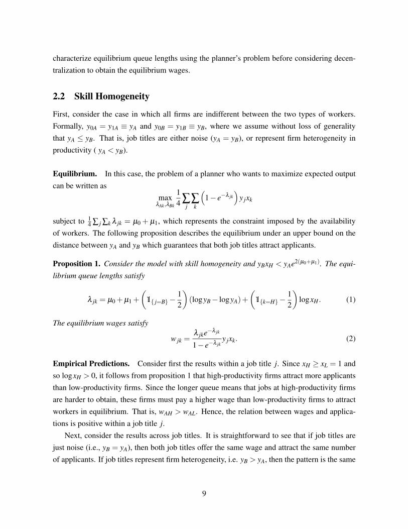
First, consider the case in which all firms are indifferent between the two types of workers.Formally, y0A = y1A ≡ yA and y0B = y1B ≡ yB, where we assume without loss of generalitythat yA ≤ yB. That is, job titles are either noise (yA = yB), or represent firm heterogeneity inproductivity ( yA < yB).

Equilibrium. In this case, the problem of a planner who wants to maximize expected outputcan be written as

maxλAk,λBk

14 ∑

j∑k

(1− e−λ jk

)y jxk

subject to 14 ∑ j ∑k λ jk = µ0 + µ1, which represents the constraint imposed by the availability

of workers. The following proposition describes the equilibrium under an upper bound on thedistance between yA and yB which guarantees that both job titles attract applicants.

Proposition 1. Consider the model with skill homogeneity and yBxH < yAe2(µ0+µ1). The equi-

librium queue lengths satisfy

λ jk = µ0 +µ1 +

(1{ j=B}−

12

)(logyB− logyA)+

(1{k=H}−

12

)logxH . (1)

The equilibrium wages satisfy

w jk =λ jke−λ jk

1− e−λ jky jxk. (2)

Empirical Predictions. Consider first the results within a job title j. Since xH ≥ xL = 1 andso logxH > 0, it follows from proposition 1 that high-productivity firms attract more applicantsthan low-productivity firms. Since the longer queue means that jobs at high-productivity firmsare harder to obtain, these firms must pay a higher wage than low-productivity firms to attractworkers in equilibrium. That is, wAH > wAL. Hence, the relation between wages and applica-tions is positive within a job title j.

Next, consider the results across job titles. It is straightforward to see that if job titles arejust noise (i.e., yB = yA), then both job titles offer the same wage and attract the same numberof applicants. If job titles represent firm heterogeneity, i.e. yB > yA, then the pattern is the same

9

as within a job title: job title B offers higher wages and attracts more applicants than job title A.That is, the relation between wages and applications is positive across job titles.

Summarizing, with skill homogeneity, job titles can only reflect differences in firm produc-tivity. In this case, the relationship between wages and the number of applicants is positive bothwithin and across job titles.

2.3 Horizontal Differentiation of Skills

We now turn to the case in which firms with job title j = A rank workers in the opposite way offirms with job title j = B, e.g. because workers’ types reflect skills that are specific to certainjob titles. For example, a cardiology nurse is different from a neurology nurse. We make twoassumptions that are without loss of generality: i) firms with job title j = A are more productivewith workers of type 0 (y0A > y1A), while firms with job title j = B produce more output withworkers of type 1 (y1B > y0B); and ii) the maximum output produced in job title A is weaklylower than the maximum output in job title B, i.e. y0A ≤ y1B.

We further assume for either job title that the less-preferred type of worker produces afraction 0 ≤ τ < 1 of the output of the most-productive workers, i.e. y1A = τy0A and y0B =

τy1B = τ . Hence, τ can be interpreted as a measure of the similarity of the skills of the twotypes of workers. For ease of exposition, we focus on the extreme τ = 0, meaning that workerscannot produce any output in the job title that does not correspond to their specialization.6

Equilibrium. If τ = 0 (or positive but sufficiently small), type-1 workers will never want toapply to job title j = A and type-0 workers will never want to apply to job title j = B. Hence,the problem of a planner who wants to maximize output can be written as

maxλ0Ak,λ1Bk

14 ∑

k

(1− e−λ0Ak

)y0Axk +

14 ∑

k

(1− e−λ1Bk

)xk

subject to 14 ∑k λ0Ak = µ0 and 1

4 ∑k λ1Bk = µ1, which represent the constraint imposed by theavailability of workers of either type. The following proposition characterizes the queue lengthsthat solve this optimization problem as well as the equilibrium wages that they imply.7

6The analysis is similar for larger values of τ . The main difference is that some workers may start applying tothe job title in which they are less productive if their output there is high or if the competition in ‘own’ job title issevere. However, the empirical predictions remain qualitatively unchanged.

7The wage of the worker type that a firm does not attract in equilibrium is not uniquely pinned down: any wagethat is sufficiently low will suffice. In practice, firms generally do not advertise wages for worker types that neverapply, so we ignore those wages here.

10

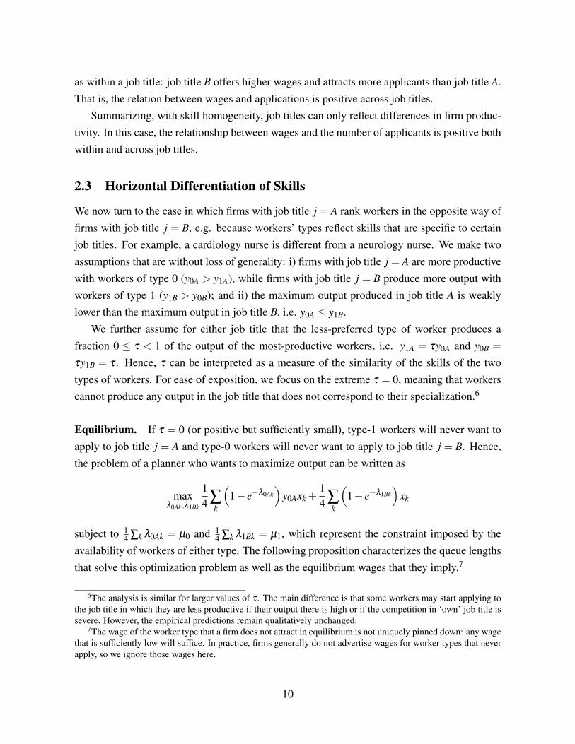
Proposition 2. Consider the model with horizontal differentiation and τ = 0. The equilibrium

queue lengths are λ1Ak = λ0Bk = 0,

λ0Ak = 2µ0 +

(1{k=H}−

12

)logxH (3)

λ1Bk = 2µ1 +

(1{k=H}−

12

)logxH . (4)

The equilibrium wages are

w0Ak =λ0Ake−λ0Ak

1− e−λ0Aky0Axk (5)

w1Bk =λ1Bke−λ1Bk

1− e−λ0Bky1Bxk. (6)

Empirical Predictions. It is straightforward to see that the empirical predictions within a jobtitle j are the same as in the case of homogeneous worker skills: high-productivity firms attractmore applicants and pay higher wages than low-productivity firms, making the relation betweenwages and applicants positive.

Next, consider the results across job titles. At a firm with job title j = A, the averagenumber of applicants is given by 1

2λ0AH + 12λ0AL, and an analogous expression holds for job

title B. As proposition 2 reveals, the ranking of this average number of applicants across jobtitles is ambiguous: job title j = B receives more applicants than job title j = A if µ1 > µ0, i.e.if there are more workers of type 1 than of type 0, and vice versa. Intuitively, since the two jobtitles are equally common and workers perfectly sort themselves, the most-prevalent skill willgenerate the longest queue.

What is the relationship between applications and wages across job titles? The number ofapplications does not depend on the productivity of the worker-job pair y (equations 3 and 4),while wages do depend on y. As a result, wages could be higher or lower in the job title withmore applications than in the job title with fewer applications, i.e. the relationship betweenapplications and wages could be positive or negative. Two forces are at play: labor markettightness and productivity. If there is no difference in productivity across job titles, i.e. y0A =

y1B, then the tightness factor dominates: wages are higher in the job with fewer applicationsbecause the job market is tighter there (and there is no competition from workers from the otherjob title). However, if productivity y is high enough in the market with lower tightness, it canoverpower the tightness effect, producing an overall positive relationship between wages andapplicants.

In a nutshell, with horizontal differentiation of job titles, the relationship between wages

11

and applications could be positive or negative depending on whether the tightness effect or theproductivity effect dominates. Empirically, for two horizontally differentiated job titles withinan occupation, productivity differences may be small, in which case the tightness effect willdominate, leading to a negative relationship between wages and applications.

2.4 Vertical Differentiation of Skills

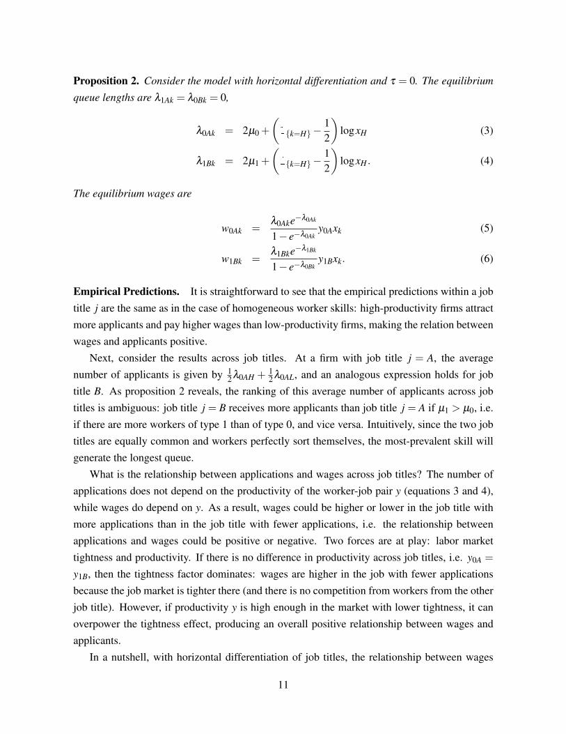
Finally, we consider the case in which all firms prefer one type of workers over the other type,e.g. workers who have more experience or are better educated are preferred by all firms. Theanalysis of vertical differentiation resembles the Faberman & Menzio (2017) adaption of themodel by Shimer (2005), but extends it by considering heterogeneity in firm productivity x.We use the terminology experienced and inexperienced to distinguish between the two types ofworkers. Without loss of generality, we assume that the experienced workers are those with typei = 1. Hence, y1 j ≥ y0 j for j ∈ {A,B}. We also assume—again without loss of generality—thatthe difference in output between inexperienced and experienced workers is (weakly) larger forfirms with job title j =B than for firms with job title j =A, i.e. θ ≡ (y1B− y0B)/(y1A− y0A)≥ 1.In line with Faberman & Menzio (2017), we will interpret θ as a measure of how sensitive jobtitle B is relative to job title A: the higher θ , the more job title B gains from hiring an experiencedworker instead of an inexperienced worker, compared to job title A. In general, we expect moresenior jobs to be more sensitive. For example, job title B could be a senior accountant and jobtitle A a junior accountant.

Equilibrium. In this scenario, the planner’s problem is

maxλi jk

14 ∑

j∑k

[(1− e−λ1 jk

)y1 j + e−λ1 jk

(1− e−λ0 jk

)y0 j

]xk,

subject to the resource constraint based on the number of workers of each type 14 ∑ j ∑k λi jk = µi

for i∈ {0,1}. The following proposition characterizes the equilibrium queue lengths and wagesunder two conditions on θ which guarantee that both job titles attract both types of workers.

Proposition 3. Consider the model with vertical differentiation, satisfying θ ∈(

y0By0A

e−2µ0, y0By0A

e2µ0

)and θ ∈

(xHe−2µ1, 1

xHe2µ1

). The equilibrium queue lengths are

λ0 jk ≡ λ0 j = µ0 +

(1{ j=B}−

12

)(logy0B− logy0A− logθ) (7)

λ1 jk = µ1 +

(1{ j=B}−

12

)logθ +

(1{k=H}−

12

)logxH . (8)

12

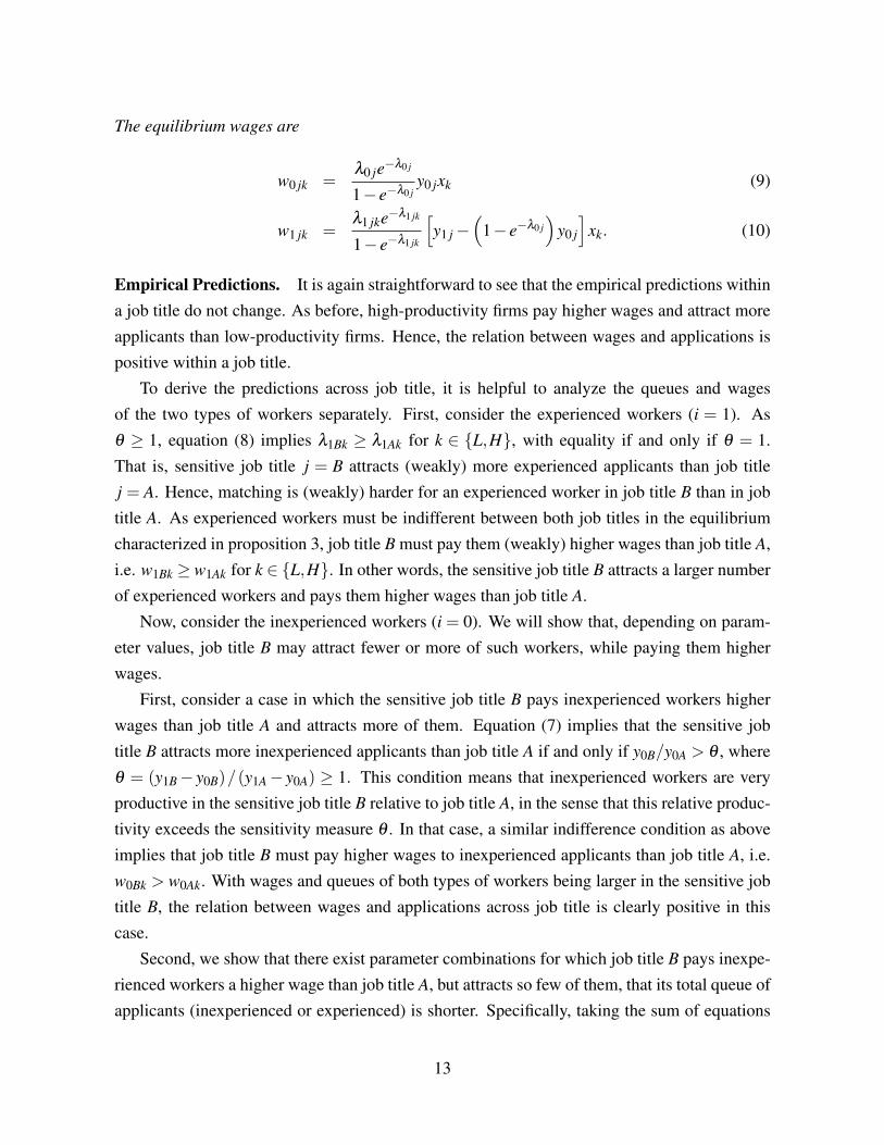
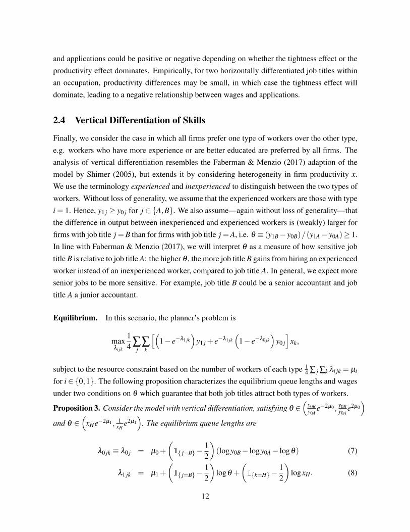
The equilibrium wages are

w0 jk =λ0 je−λ0 j

1− e−λ0 jy0 jxk (9)

w1 jk =λ1 jke−λ1 jk

1− e−λ1 jk

[y1 j−

(1− e−λ0 j

)y0 j

]xk. (10)

Empirical Predictions. It is again straightforward to see that the empirical predictions withina job title do not change. As before, high-productivity firms pay higher wages and attract moreapplicants than low-productivity firms. Hence, the relation between wages and applications ispositive within a job title.

To derive the predictions across job title, it is helpful to analyze the queues and wagesof the two types of workers separately. First, consider the experienced workers (i = 1). Asθ ≥ 1, equation (8) implies λ1Bk ≥ λ1Ak for k ∈ {L,H}, with equality if and only if θ = 1.That is, sensitive job title j = B attracts (weakly) more experienced applicants than job titlej = A. Hence, matching is (weakly) harder for an experienced worker in job title B than in jobtitle A. As experienced workers must be indifferent between both job titles in the equilibriumcharacterized in proposition 3, job title B must pay them (weakly) higher wages than job title A,i.e. w1Bk ≥ w1Ak for k ∈ {L,H}. In other words, the sensitive job title B attracts a larger numberof experienced workers and pays them higher wages than job title A.

Now, consider the inexperienced workers (i = 0). We will show that, depending on param-eter values, job title B may attract fewer or more of such workers, while paying them higherwages.

First, consider a case in which the sensitive job title B pays inexperienced workers higherwages than job title A and attracts more of them. Equation (7) implies that the sensitive jobtitle B attracts more inexperienced applicants than job title A if and only if y0B/y0A > θ , whereθ = (y1B− y0B)/(y1A− y0A) ≥ 1. This condition means that inexperienced workers are veryproductive in the sensitive job title B relative to job title A, in the sense that this relative produc-tivity exceeds the sensitivity measure θ . In that case, a similar indifference condition as aboveimplies that job title B must pay higher wages to inexperienced applicants than job title A, i.e.w0Bk > w0Ak. With wages and queues of both types of workers being larger in the sensitive jobtitle B, the relation between wages and applications across job title is clearly positive in thiscase.

Second, we show that there exist parameter combinations for which job title B pays inexpe-rienced workers a higher wage than job title A, but attracts so few of them, that its total queue ofapplicants (inexperienced or experienced) is shorter. Specifically, taking the sum of equations

13

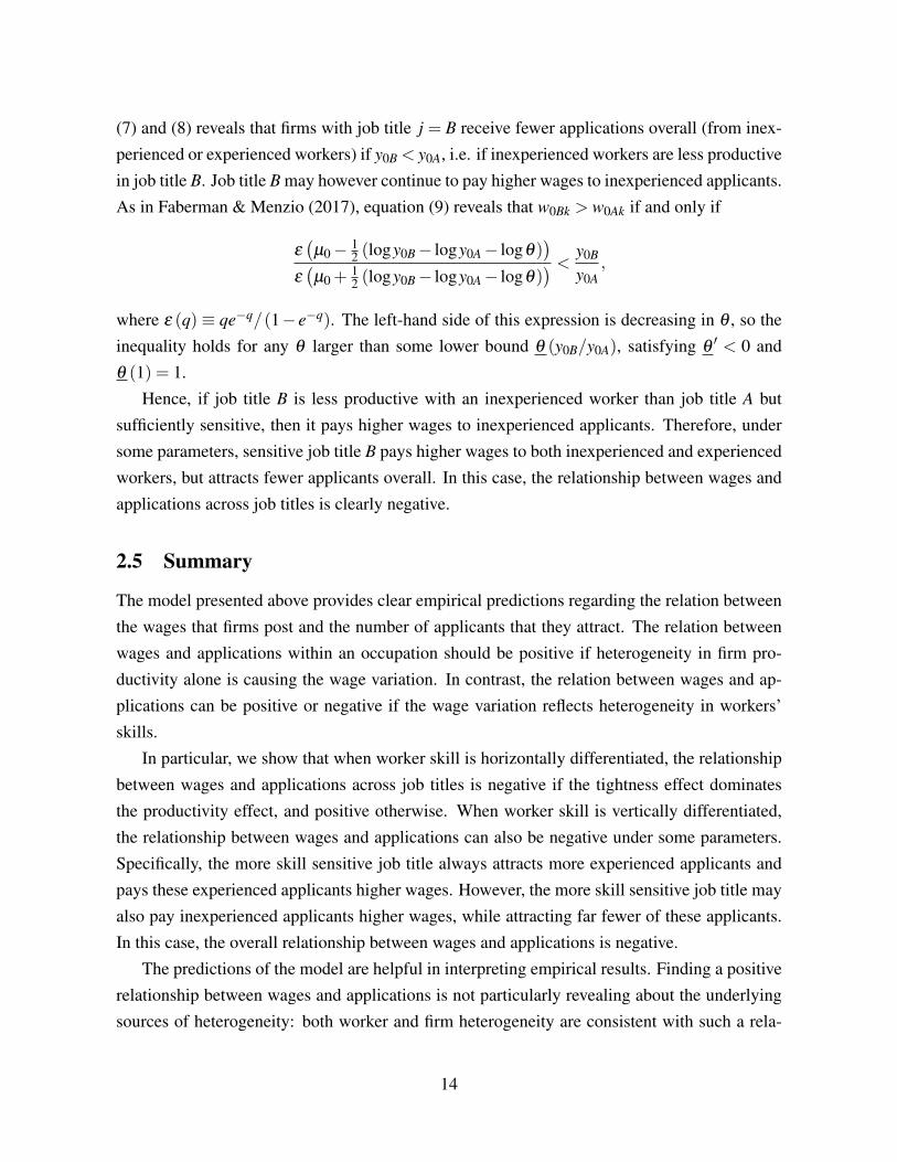
(7) and (8) reveals that firms with job title j = B receive fewer applications overall (from inex-perienced or experienced workers) if y0B < y0A, i.e. if inexperienced workers are less productivein job title B. Job title B may however continue to pay higher wages to inexperienced applicants.As in Faberman & Menzio (2017), equation (9) reveals that w0Bk > w0Ak if and only if

ε(µ0− 1

2 (logy0B− logy0A− logθ))

ε(µ0 +

12 (logy0B− logy0A− logθ)

) < y0B

y0A,

where ε (q) ≡ qe−q/(1− e−q). The left-hand side of this expression is decreasing in θ , so theinequality holds for any θ larger than some lower bound θ (y0B/y0A), satisfying θ

′ < 0 andθ (1) = 1.

Hence, if job title B is less productive with an inexperienced worker than job title A butsufficiently sensitive, then it pays higher wages to inexperienced applicants. Therefore, undersome parameters, sensitive job title B pays higher wages to both inexperienced and experiencedworkers, but attracts fewer applicants overall. In this case, the relationship between wages andapplications across job titles is clearly negative.

2.5 Summary

The model presented above provides clear empirical predictions regarding the relation betweenthe wages that firms post and the number of applicants that they attract. The relation betweenwages and applications within an occupation should be positive if heterogeneity in firm pro-ductivity alone is causing the wage variation. In contrast, the relation between wages and ap-plications can be positive or negative if the wage variation reflects heterogeneity in workers’skills.

In particular, we show that when worker skill is horizontally differentiated, the relationshipbetween wages and applications across job titles is negative if the tightness effect dominatesthe productivity effect, and positive otherwise. When worker skill is vertically differentiated,the relationship between wages and applications can also be negative under some parameters.Specifically, the more skill sensitive job title always attracts more experienced applicants andpays these experienced applicants higher wages. However, the more skill sensitive job title mayalso pay inexperienced applicants higher wages, while attracting far fewer of these applicants.In this case, the overall relationship between wages and applications is negative.

The predictions of the model are helpful in interpreting empirical results. Finding a positiverelationship between wages and applications is not particularly revealing about the underlyingsources of heterogeneity: both worker and firm heterogeneity are consistent with such a rela-

14

tionship. However, a negative relationship between wages and applications is consistent with animportant role for worker heterogeneity, either horizontal or vertical. Furthermore, in the con-text of vertical heterogeneity, job titles with higher wages but fewer applicants can be identifiedas sensitive job titles, where the benefits of hiring more experienced workers are greater.

In the remainder of this paper, we will argue that data from CareerBuilder.com supports ourmodel and is consistent with the idea that job titles reflect how firms value workers’ heteroge-neous skills.

3 Data

To analyze the relation between wages and the pool of applicants within and across job titles,we use proprietary data provided by CareerBuilder.com. In this section, we describe the mainfeatures of our data set.

Background. CareerBuilder is the largest online job board in the United States, visited by ap-proximately 11 million unique job seekers during January 2011.8 While job seekers can use thesite for free, CareerBuilder charges firms several hundred dollars to post a job ad on the websitefor one position for one month. A firm that wishes to keep the ad online for another month issubject to the same fee, while a firm that wishes to advertise multiple positions needs to payfor each position separately, although small quantity discounts are available (see CareerBuilder,2013). At each moment in time, the CareerBuilder website contains over 1 million jobs.9

Search Process. A firm posting a job is asked to provide various pieces of information. First,it needs to specify a job title, e.g. “senior accountant,” which will appear at the top of thejob posting as well as in the search results. CareerBuilder encourages the firm to use simple,recognizable job titles and avoid abbreviations, but firms are free to choose any job title theydesire. Further, the firm provides the full text of the job ad, a job category and industry, and thegeographical location of the position. Finally, the firm can specify education and experiencerequirements as well as the salary that it is willing to pay.

A job seeker who visits CareerBuilder.com sees a web form which allows him to specifysome keywords (typically the job title), a location, and a category (broad type of job selected

8See comScore Media Metrix (2011). Monster.com is similar in size, and whether Monster or CareerBuilder islarger depends on the exact measure used.

9Our data is limited to search activity on CareerBuilder. We therefore miss information on search activities onother employment websites or offline. See e.g. Nakamura et al. (2008), Stevenson (2008) and Kuhn & Mansour(2014) for studies of search behavior across platforms.

15

from a drop-down menu). After providing this information10, the job seeker is presented a listof vacancies matching his query, organized into 25 results per page. For the jobs that appear inthe list, the job seeker can see the job title, salary, location, and the name of the firm. To getmore details about a job, the worker must click on the job snippet in the list, which brings themto a page with the full text of the job ad as well as a “job snapshot” summarizing the job’s keycharacteristics. At the top and bottom of each job ad, a large “Apply Now” button is present,which brings the worker to a page where they can send their resume and their cover letter to theemployer.

Sample. Our data set consists of vacancies posted on CareerBuilder in the Chicago and Wash-ington, DC Designated Market Areas (DMA) between January and March 2011. A DMA is ageographical region set up by the A.C. Nielsen Company that consists of all the counties thatmake up a city’s television viewing area. DMAs are slightly larger in size than MetropolitanStatistical Areas and they include rural zones. Our data is a flow sample: we observe all vacan-cies posted in these two locations during January and February 2011 and we observe a randomsubsample of the vacancies posted in March 2011.

Variables. The CareerBuilder data is an attractive source of information compared to existingdata sets, in particular due to the large number of variables that it includes. For each vacancy,we observe the following job characteristics: the job title, the salary (if specified), whether thesalary is hourly or annual, the education level required for the position, the experience levelrequired for the position, an occupation code, and the number of days the vacancy has beenposted. The occupation code is the detailed, six-digit O*NET-SOC (Standard OccupationalClassification) code.11 CareerBuilder assigns this code based on the full content of the job adusing O*NET-SOC AutoCoder, the publicly available tool endorsed by the Bureau of LaborStatistics.12 This procedure is consistent with the approach of commonly used labor marketsurveys, such as the Current Population Survey (CPS).13 We further observe the following firm

characteristics: the name of the firm, an industry code, and the total number of employees inthe firm. CareerBuilder uses external data sets, such as Dun & Bradstreet, to match the two-digit NAICS (North American Industry Classification System) industry code and the number ofemployees of the firm to the data.

10It is not necessary to provide information in all three fields.11See http://www.onetcenter.org/taxonomy.html. We henceforth refer to this classification simply as

SOC.12See http://www.onetsocautocoder.com/plus/onetmatch.13This means that misclassification is unlikely to be a larger problem in the CareerBuilder data than in the CPS.

See Mellow & Sider (1983) for an analysis of inconsistencies in occupational codes in the CPS.

16

In addition to these characteristics, we also observe several outcome variables for eachvacancy. Our first outcome variable, the number of views, represents the number of times thata job appeared in a listing after a search. The second outcome variable, the number of clicks,is the number of times that a job seeker clicked on the snippet to see the entire job ad. Finally,we observe the number of applications to each job, where an application is defined as a personclicking on the “Apply Now” button in the job ad.

From these numbers, we construct two new variables that reflect applicant behavior: thenumber of applications per 100 views, and the number of clicks per 100 views. These measurescorrect for heterogeneity in the number of times a job appears in a listing, allowing us to analyzeapplicants’ choices among known options.

For a random subset of the vacancies of January and March 2011, we also observe someapplicant characteristics. Specifically, we observe the number of applicants broken down byeducation level (if at least an associate degree) and by general work experience (in bins of5 years). We will use these job seeker characteristics as proxies for worker productivity toanalyze the quality of the applicant pool that a firm attracts.

Cleaning. We express all salaries in yearly amounts, assuming a full-time work schedule.When a salary range is provided, we use the middle of the interval for most of the analysis,but we perform robustness checks in section 5. To reduce the impact of outliers and errors, weclean the wage data by removing the bottom and top 0.5% of the salaries.

Because job titles are free-form, many unique ones exist and the frequency distribution ishighly skewed to the right. To improve consistency, we cleaned the data. Most importantly, weformatted every title in lower case and removed any punctuation signs, employer names, or joblocations. In most of our analysis, we restrict attention to the first four words of a job title. Aswe will discuss, because this restriction has minimal impact on the number of unique job titlesin our sample, our results are not sensitive to it.

Representativeness. Some background work (data not shown) was done to compare the jobvacancies on CareerBuilder.com with data on job vacancies in the representative JOLTS (JobOpenings and Labor Turnover Survey). The number of vacancies on CareerBuilder.com rep-resents 35% of the total number of vacancies in the US in January 2011 as counted in JOLTS.Compared to the distribution of vacancies across industries in JOLTS, some industries are over-represented in the CareerBuilder data, in particular information technology; finance and insur-ance; and real estate, rental, and leasing. The most underrepresented industries are state andlocal government, accommodation and food services, other services, and construction.

17

While CareerBuilder data is not representative by industry, in most other respects it is rep-resentative of the US labor market, as documented by Marinescu & Rathelot (2018). Using arepresentative sample of vacancies and job seekers from CareerBuilder.com in 2012, they showthat the distribution of vacancies across occupations is essentially identical (correlation of 0.95)to the distribution of vacancies across all jobs on the Internet as captured by the Help WantedOnline data. Furthermore, the distribution of unemployed job seekers on CareerBuilder.comacross occupations is similar to that of the nationally representative Current Population Survey(correlation of more than 0.7). Hence, the vacancies and job seekers on CareerBuilder.com arebroadly representative of the US economy as a whole, and they form a substantial fraction ofthe market.

Descriptive Statistics. Table 1 shows the summary statistics for our sample. The full sampleconsists of more than 60,000 job openings by 4,797 different firms. On average, each job wasonline for 16 days, during which it was viewed as a part of a search result 6,084 times, received281 clicks, and garnered 59 applications. Per 100 views, the average job receives almost sixclicks and approximately one application.14

Only a minority of job ads include an explicit experience requirement (0.3%) or an expliciteducation requirement (42%). When specified, these requirements appear in the “job snapshot”box at the end of the full job ad, but they do not appear in the job snippet that job seekers first seein the search results. Therefore, employers may choose not to fill in education and experiencerequirements if they feel that the overall job description is sufficiently informative.15

We observe a posted wage for approximately 20% of the jobs. When present, the wagedoes appear in the job snippet as part of the search results. The average posted yearly salaryis just over $57,000, and we will show in more detail below that posted wages on the websitehave the same distribution as the wages of full-time workers in the Current Population Survey.In the smaller sample with posted wages, there are 1,369 unique firms. Finally, we observe theaverage applicant quality for approximately 2,300 positions. The average applicant has between16 and 17 years of education (conditional on holding at least an associate degree) and just over13 years of work experience.

Job Titles. All job ads in our sample specify a job title. This job title is prominently featuredon the employment website and is the main piece of information that workers use to search theCareerBuilder database. The full sample of more than 60,000 job openings contains 22,009

14Keep in mind that the average of ratios does not necessarily need to equal the ratio of averages.15In an alternative data set, Hershbein & Kahn (2016) find that as much as half of all firms post an education

and/or experience requirement.

18

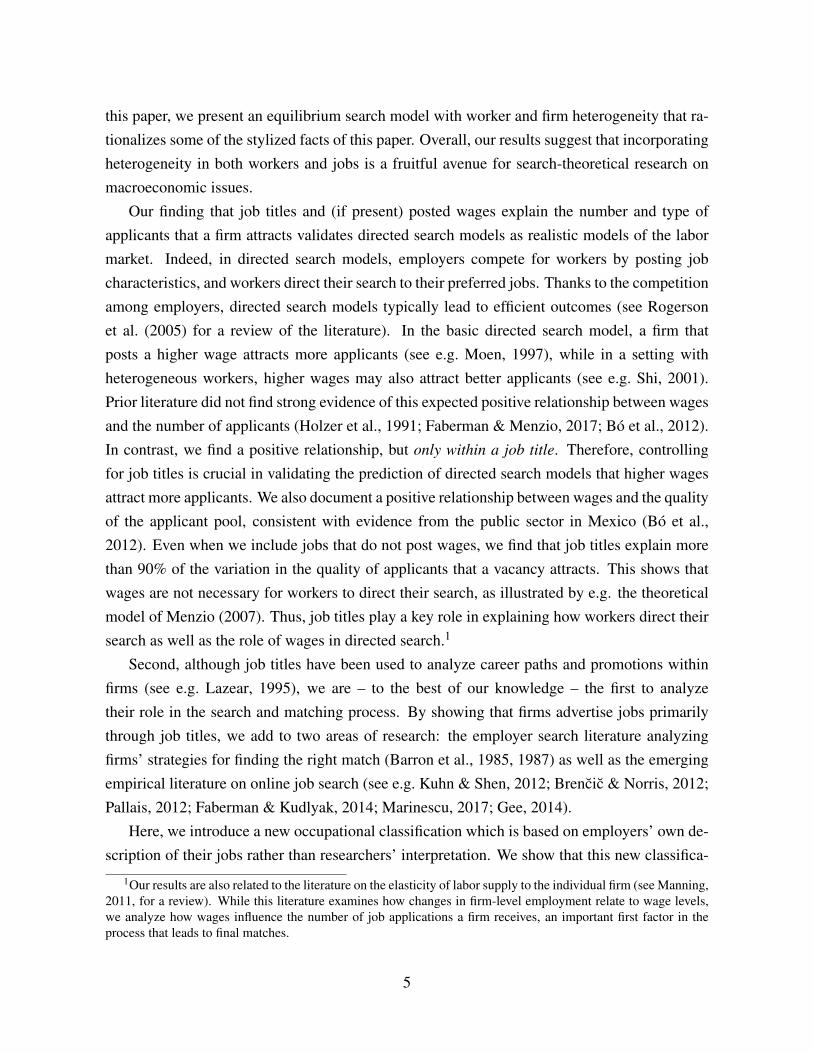
unique job titles. Truncation to the first four words marginally reduces this number to 20,447.In the subsample of jobs with posted wages, the corresponding numbers are 4,669 and 4,553,respectively. In Table 2, we list the ten most common job titles (after truncation), both for thefull sample and for the subsample of jobs that post wages. Note that the most common job titlesare typically at most three words long. We also show the most common job titles if we truncatethe job title to the first two words or the first word. Figure 1 provides a more comprehensiveoverview of frequent job titles in the form of a word cloud, in which the size of a job titledepends on its frequency.

Inspection of the table and the figures reveals that job titles often describe occupations, e.g.“administrative assistant,” “customer service representative,” or “senior accountant.” This raisesthe question of how job titles compare to other definitions of occupations, in particular the oc-cupational classification (SOC) of the Bureau of Labor Statistics. Since our data includes SOCcodes, we can explicitly make this comparison. Perhaps the most obvious difference betweenjob titles and SOC codes concerns their variety: in our full sample, the number of unique jobtitles is more than 25 times the number of unique SOC codes.16 In other words, job titles pro-vide a finer classification. For example, they distinguish between “inside sales representative”and “outside sales representative,” between “executive assistant” and “administrative assistant,”and between “senior accountant” and “staff accoutant”—while each of the two jobs in thesepairs would have the same SOC code. While some of the larger variety in job titles might bedue to noise in employers’ word choice, we will show in the following sections that distinctionsbetween job titles are economically significant.

4 Empirical Analysis

Our empirical analysis consists of two parts. First, we analyze to what extent the wage that afirm posts affects its number of applicants. Subsequently, we analyze the effect of the wage onthe average quality of applicants.

4.1 Number of Applicants

Table 3 presents our first set of results. As we discuss in more detail below, the set of controlsvaries across the columns, with log wages always being included. The dependent variable in

1620,447 versus 762, to be exact. In the subsample with posted wages, the difference is smaller, but still a factorof eight (4,553 versus 594). Note that the SOC classification distinguishes 840 occupations in total, some of whichdo not appear in our data.

19

each specification is the number of applications per 100 views, which we use to correct forheterogeneity in the number of views across jobs.17

4.1.1 Wage Impact

Across Job Titles. We start by exploring the relation between the wage and the number ofapplicants without any additional controls (column I). This cross-sectional relationship is sig-nificantly negative in our sample: a 10% increase in the wage is associated with a 6.3% declinein applications per view.18 Of course, we cannot draw too many conclusions from this result.As highlighted by our model, there is no a priori reason to expect a particular sign when we donot control for relevant heterogeneity: it is perfectly possible that a firm looking for a lawyeroffers a higher wage but attracts fewer applicants than a firm looking for a janitor.

More interestingly, however, we find that the negative association between wages and thenumber of applicants is actually quite robust. In particular, it survives if we add controls thatare commonly used to capture labor market heterogeneity, such as job characteristics as well asdetailed occupation fixed effects (column II) and firm fixed effects (column III). These controlsindeed explain part of the variance in the number of applicants, as demonstrated by the increasein the R2, but the coefficient on the wage and its significance remain essentially unchanged: incolumn III, an 10% increase in the wage offer is associated with a statistically significant 5.8%decline in the number of applications per view.

Within Job Titles. As our model indicates, the negative relationship of column III could stillbe the result of omitted variable bias: within an occupation and a firm, relevant heterogeneitymay still exist and the failure to control for this heterogeneity affects the estimate of the wagecoefficient. As job titles appear to provide a finer classification of jobs than SOC codes, it seemsnatural to expect that they may capture part of this heterogeneity.

We test this hypothesis in column IV and V by replacing the SOC code fixed effects with jobtitle fixed effects, allowing us to consider the relation between wages and applications within ajob title. As these columns show, this exercise yields fundamentally different results. In partic-ular, the negative relationship between wages and the number of applications seen in columnsI, II, and III now becomes significantly positive. That is, within job title, higher wages are asso-ciated with more applicants. This is true regardless of whether we include firm fixed effects or

17An alternative choice for the outcome variable is simply the logarithm of the number of applicants for eachjob. We find that our key results from Table 3 are qualitatively unaffected by this alternative outcome definition.

18A 10% increase in the wage decreases the number of applications per 100 views by 0.770log(1.1) = 0.073,which is a 6.3% decline compared to the sample average of 1.168.

20

not. The point estimate in column V implies that a 10% increase in the wage is associated witha 7.7% increase in the number of applicants per 100 views.

As the R2 indicates, the specifications with job title fixed effects explain a larger part of thevariation in the number of applicants per view. At some level, this is not surprising as there aremany more job titles than occupations. However, that is not the full story since measures thatcorrect for the larger number of controls, such as the adjusted R2 and the AIC, also favor thespecifications with job titles. The combination of these results strongly suggests that job titlescapture meaningful worker heterogeneity that is glossed over by standard occupational codes.

4.1.2 Word Analysis

While it is informative to know that controlling for job title fixed effects reverses the sign of therelationship between wages and the number of applicants, this fact in itself does not reveal whatheterogeneity is captured by job titles. To better understand the explanatory power of job titles,we use fixed effects for the separate words in a job title.

Specifically, we regress wages and the number of applicants per view on detailed SOCcodes, compute the residuals, and regress those residuals on a set of dummy variables for eachword appearing in the job title. Compared to job title fixed effects, this specification is restrictivebecause it ignores the order and combinations in which words appear in a job title; it assumes,for example, that the word “assistant” has the same effect in “executive assistant” and “assistantstore manager”. Yet, this specification allows us to determine which words are most important.

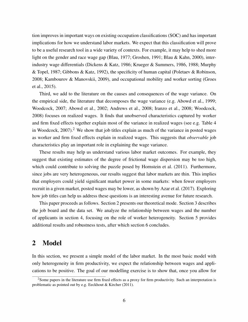
Wages. First, we explore which words are most important in explaining wages. In Table 4,we list words that appear at least 100 times and are significant at least at the 5% level. Wechecked the job titles in which these words appear and manually classified the words into threecategories.

The first column includes words that suggest the presence of vertically differentiated skillswithin an SOC code, as these words signal the seniority of the worker holding this job title.Within an SOC code, job titles that include the words “manager” or “senior” have higher thanaverage posted wages, whereas wages are lower than average for titles that include the words“specialist” or “junior”. For instance, within the SOC code 13-2011 (“Accountants and Audi-tors”), accounting managers and senior accountants earn more than accounting specialists andjunior accountants.

In the second column, we list words that suggest the presence of horizontally differenti-ated skills within an SOC, as these words capture specialties or skills. For example, within theSOC code 41-3099 (“Sales Representatives, Services, All Other”) or 41-4012 (“Sales Repre-

21

sentatives, Wholesale and Manufacturing, Except Technical and Scientific Products”), insidesales jobs, which require employees to contact customers by phone, pay less than outside salesjobs, where employees must travel and meet face-to-face with customers.19 Finally, the thirdcolumn is similar to the second column, but focuses on computer skills and specialties. For ex-ample, within SOC code 15-1071 (“Network and Computer Systems Administrators”), networkadministrators earn less than systems administrators.

Figure 2 provides a more complete overview of the words that are associated with eitherhigher or lower wages. The size of the words represents their frequency, while the intensityof the color represents the magnitude of their effect. We can classify the words in this figurein roughly the same way as the frequent words from Table 4. For example, “president” and“intern” indicate very different levels of seniority and have opposing effects on the wage withinan SOC, just as one would expect. “Scientist” and “retail” are examples of skills/specialtiesleading to a higher and a lower wage, respectively. Finally, in terms of computer skills, theword “linux” is associated with higher wages, while the generic term “computer” leads to lowerwages within an SOC.

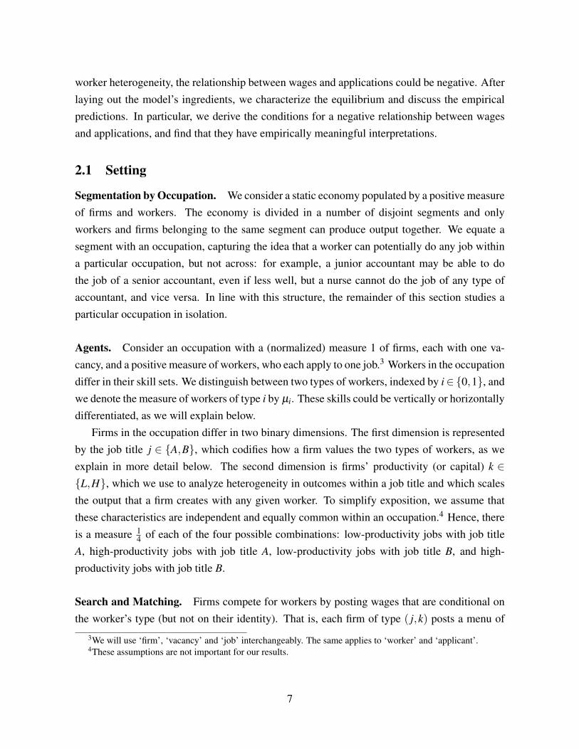
Applications. We now discuss words that are associated with a larger or smaller number ofapplicants per view within SOC code (Figure 3). Many of the words that predict a greaternumber of applicants per view are also words that predict lower wages (compare with Figure 2).These include words denoting lower seniority and experience (vertical differentiation), such as“assistant”, “support”, “specialist”, “coordinator”, “entry”, and “junior”. As for words denotingspecialties (horizontal differentiation), we can see, for example, that lower-wage inside salesjobs receive more applications than the average job in the same SOC.

Conversely, many of the words that predict a lower number of applicants per view withinSOC are words that also predict higher wages. The two word clouds are remarkably similar.Words that denote higher seniority and management positions such as “manager”, “senior”, and“director” are associated with a smaller number of applicants. Words that are associated withhigher paying specialties or areas, such as “developer”, “engineer”, and “linux”, have a lowernumber of applicants.

Overall, examining the words that predict wages and words that predict the number of ap-plicants enlightens us on the negative relationship between wages and applicants within SOC.

19The most frequent word among those that are associated with higher wages in the second column is "-". Thisis not a typo; this character typically separates the main job title from additional details about the job. Theseadditional details were deemed important enough for the firm to specify them in the job title. Presumably, all otherthings equal, a more specialized job comes with a higher pay. Some examples of the use of "-" are: "web developer- c# developer - net developer - vb net developer" or "web developer - ruby developer - php developer - ror pearljava".

22

Within SOC, words in the job title associated with higher wages predict a lower number of ap-plicants per view, and vice versa for words in the job title associated with lower wages. Substan-tively, jobs with higher seniority or managerial responsibilities (vertical differentiation) tend topay higher wages and attract fewer applicants. Similarly, specialties (horizontal differentiation)with higher pay tend to attract fewer applicants.

4.1.3 Interpretation

We interpret our results as indicating that the negative relationship between wages and appli-cations found when using SOC codes reflects significant heterogeneity between workers in agiven SOC. Jobs with the same SOC code can still differ, e.g. in how they value the skill set of aparticular worker. These differences directly affect both the wage and the number of applicants,rendering estimates obtained without controlling for this heterogeneity inconsistent.

Our results further indicate that job titles capture part of this heterogeneity. In particular,we find that words describing vertical or horizontal differences in workers’ skills are oftenassociated with either a higher wage and a lower number of applicants, or vice versa.

Our model provides a clear way to interpret these results. For example, the negative re-lationship among jobs with horizontally differentiated skill requirements such as “inside salesrepresentative” and “outside sales representative” support the idea that the tightness effect dom-inates the productivity effect. If there is higher demand for outside sales representatives relativeto supply, then the tightness effect20 predicts both higher wages and a lower number of ap-plicants for outside sales representatives. To overpower this tightness effect, the productivityof inside sales representatives has to high enough relative to the productivity of outside salesrepresentatives. Given that the relationship between wages and applications is negative, we con-clude that there is more demand for outsides sales representatives relative to supply, and thereis no marked productivity advantage for inside sales representatives relative to outside salesrepresentatives.

Further, the negative relationship among jobs with vertically differentiated skill require-ments such as “senior accountant” and “junior accountant” supports the idea that these jobsdiffer in their sensitivity, with the productivity of an inexperienced worker being particularlylow in the more senior job.

Our finding that “manager” is a sensitive job type is consistent with the literature on theimpact of management on firm performance. Indeed, Bloom et al. (2016) show that differencesin management practices account for about 30% of total factor productivity differences across

20In fact, Davis & Marinescu (2018) show that labor market tightness measured as vacancies over applicationshas a positive impact on posted wages in data from CareerBuilder.com.

23

firms. Therefore, it makes sense that hiring a better manager over a worse one is more importantthan hiring a better “junior” person over a worse one.

Beyond managers, the word clouds suggest that other types of jobs such as senior jobs aresensitive, while assistant, associate, junior or coordinator are more regular jobs. In fact, theliterature on management shows that one of the distinctive features of good management ishiring the right people (Bender et al., 2017). Overall, our findings suggest that manager andsenior jobs are sensitive, so hiring the right worker in in these positions can make a substantialdifference to firm productivity.

4.2 Quality of Applicants

To examine the quality of the applicants that a vacancy attracts, we use two different measuresof the quality of an applicant pool: i) the average level of work experience among applicants,and ii) the average education level among applicants, expressed in years of education.

4.2.1 Wage Impact

Average Experience. Table 5 displays the results for the average experience level. Not sur-prisingly, we find that in the cross-section higher wages are associated with more experiencedapplicants (column III). More interestingly, the relation survives once we control for job titlefixed effects (column IV) although both the magnitude and the significance level are somewhatreduced.21 If we additionally control for job characteristics (column V), the magnitude of theeffect and its significance slightly increase again. To be precise, the specification in column Vwith job title fixed effects and job characteristics indicates that a 10% increase in the wage isassociated with an increase in the experience of the average applicant by 0.15 years, or roughly1%.

Average Education. In Table 6, we focus on the education level of the average applicant.22

The results are very similar to what we found when explaining the experience of the averageapplicant. First, higher wages are associated with more educated applicants in the cross-section(column III). Second, after controlling for job title fixed effects and job characteristics, thiseffect remains although the magnitude and the significance are somewhat reduced (column VI

21One factor that may affect the significance of our estimates is the relatively small sample size and the largenumber of job titles. Note further that job titles already explain most of the variation in the average experiencelevel for both all jobs (column I) and the sample of jobs that post a wage (column II)(R2=0.96).

22See also Kudlyak et al. (2012) for evidence on how different jobs attract workers with different levels ofeducation.

24

and V). Quantitatively, the effect is small with a 10% increase in the wage being associated withan increase in the number of years of education of less than 1% within a job title.23

4.2.2 Word Analysis

As before, we develop a better understanding for the importance of job titles by investigatingwhich words are particularly important for explaining the variation in the quality of applicantswithin an SOC code. Because the sample size for this exercise is much smaller, we report theresults in Table 7 rather than a word cloud.

Words that predict higher experience or higher education tend to be words that also predicthigher wages, and vice versa for words that predict lower experience or education. For exam-ple, words that indicate higher seniority or management such as “manager” and “senior” areassociated with higher experience, while words like “director” and “chief” are associated withboth higher experience and higher education. Lower education and experience are associatedwith certain specialties. The example of “rn" (registered nurse) is interesting, as it is associatedwith both lower experience and lower education. This is explained by the fact that, within SOC29-1111 (“Registered Nurses”), “rn” indicates a lower level job compared to job titles where“rn” does not appear, such as “nurse manager,” “nurse clinician,” and “director of nursing.”

4.2.3 Interpretation

Our word analysis shows that words predicting more (less) experience or education tend to bewords that also predict higher (lower) wages. This explains why the effect of the wage onexperience (Tables 5) and education (Table 6) is reduced once we control for job title fixedeffects.

These results are in line with our model for jobs with vertically differentiated skill require-ments. Higher education or experience corresponds to the notion of more “experienced” work-ers in the model: such workers are preferred by all firms. When sensitive jobs (e.g. “senioraccountant”) pay higher wages but receive fewer applicants than non-sensitive jobs (e.g. “ju-nior accountant”), our model predicts that the sensitive job should attract an applicant pool thatis more “experienced” on average. This is exactly what we observe for words like “senior”,“manager”, “director”, “executive”, “management”, et cetera. The fact that a positive corre-lation between wages and the quality of applicants exists within a job title is also consistentwith our model with vertically differentiated skills: more productive firms within a job title payhigher wages and attract more experienced workers, as shown in proposition 3.

23Job titles alone again explain most of the cross-sectional variation in the average education level among bothall jobs (column I) and the sample of jobs that post a wage (column II)

25

5 Additional Results and Robustness

In this section, we present a number of additional results and robustness checks. First, weexplore the external validity of our sample, since our results so far are based on the 20% subsetof job ads containing an explicit announcement regarding the wage.24 To investigate how thissubset compares to the rest of the sample, we analyze firms’ decision to post a wage or not, aswell as firms’ decision of how much to offer, conditional on posting a wage. Subsequently, weprovide a robustness check on our central result by exploring the relation between wages andthe number of times potential applicants click on a job ad for more info (as opposed to applyingto the job).

5.1 Wage Posting

Cross-Sectional Variance. Table 8 displays our results regarding whether firms post a wageor not. Using a linear probability model, we find that both job titles (column I) and firm fixedeffects (column II) have high explanatory power for the decision to post a wage: they eachexplain around 70% of the variance in wage-posting behavior. Including both simultaneouslyessentially explains all of the variation in job posting behavior (the R2 is 0.93 in column III).

Including additional job characteristics improves the model fit only slightly (column IV),although some characteristics have a statistically significant impact on the posting decision. Forexample, jobs that require a high school degree or a 4-year college degree are significantly morelikely (5 and 1 percentage points, respectively) to post a wage than jobs that require a 2-yearcollege degree. On the other hand, jobs that require a graduate degree are significantly lesslikely (3 percentage points) to post a wage than jobs that require a 2-year college degree. Jobsthat do not specify an education requirement are also less likely to post a wage (2 percentagepoints). While the effect of education on posting the wage is non-linear, the pattern is consistentwith the findings of Brencic (2012) that jobs with higher skill requirements are less likely to postwages if we just compare high school jobs to jobs with higher educational requirements.

24Various explanations for this number are possible. Some firms may not wish to commit to a particular wage exante (see e.g. Michelacci & Suarez, 2006, for an equilibrium model). Some firms may feel that the combination ofthe job title and the text in the ad provide job ad provide sufficiently precise information on compensation such that,in equilibrium, firms consider it unnecessary to also post a wage. An additional explanation might be the fact thatsome companies use Applicant Tracking Systems (ATS) software that keeps track of job postings and applications.This software typically removes the wage information by default before sending out the job posting to online jobboards such as CareerBuilder (private communication with CareerBuilder.com). However, this is unlikely the fullstory. First, the fact that most job ads do not advertise wages is consistent with the worker survey data of Hall &Krueger (2012) and evidence from job boards in other countries where ATS may be less common (Brencic, 2012;Kuhn & Shen, 2012). Second, if firms really cared about advertising wages, it would be suboptimal for them torely on software that removes this information.

26

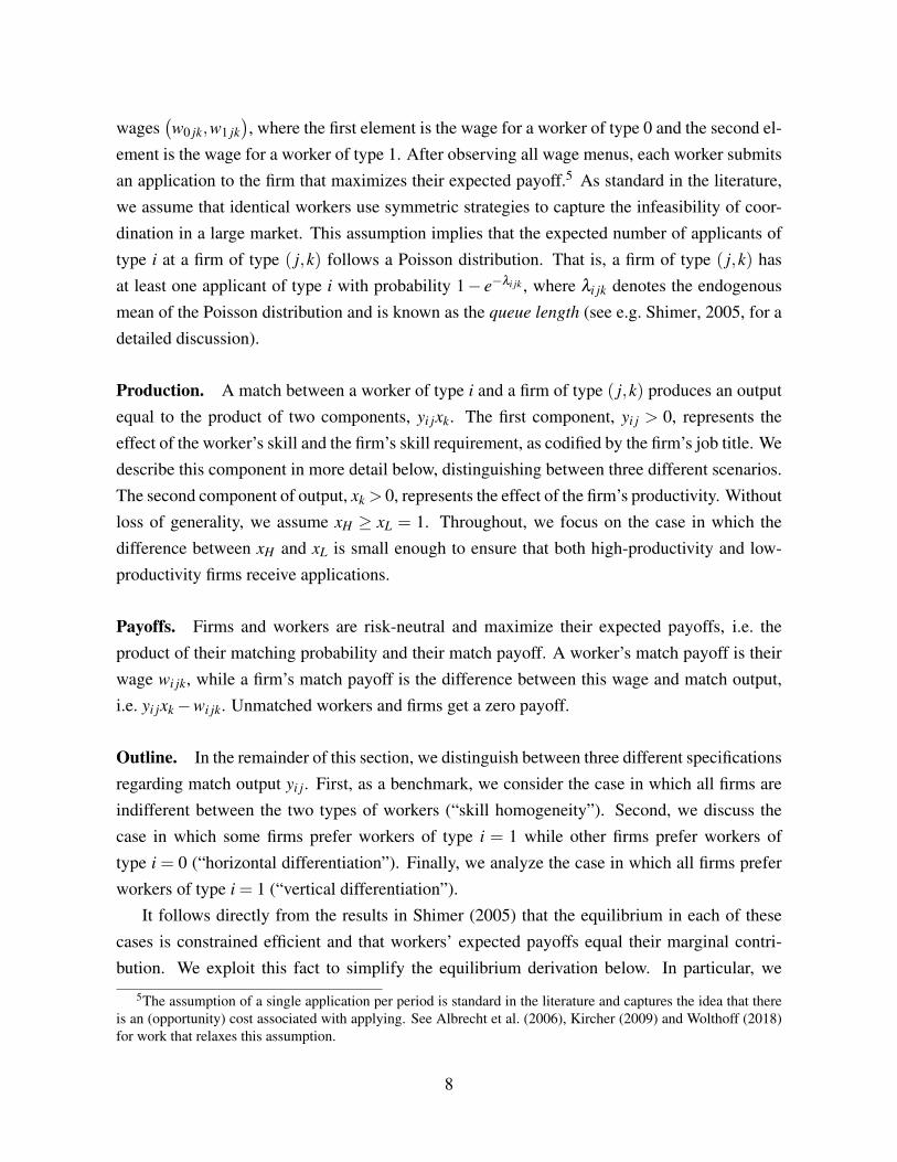
Word Analysis. The words that significantly increase or decrease the probability that a job adcontains a wage are displayed in Figure 4. Unlike the figure for the wage level, this figure doesnot show a clear pattern. In particular, both “high-wage” words and “low-wage” words (fromFigure 2) can predict a higher probability of posting a wage. For example, if we consider wordsindicating seniority, then both “manager” (higher wage) and “junior” (lower wage) increase theprobability that a wage is present in the ad, while “chief” (higher wage) and “representative”(lower wage) decrease this probability. If we consider words indicating specialization, thenboth “web” (higher wage) and “retail” (lower wage) increase the probability of posting a wage,while both “-” (higher wage) and “associate” (lower wage) decrease the probability of postinga wage.

5.2 Wage Offers

Since not all firms post a wage (for more discussion of wage posting on online plaforms, seealso Kuhn & Shen, 2012; Brencic, 2012; Brown & Matsa, 2014) and since posted wages are notnecessarily all accepted, a natural question is how the distribution of posted wages on Career-Builder compares to the cross-sectional distribution of realized (i.e. accepted) wages in the US.To answer this question, we use data from the basic monthly CPS from January and February2011. We restrict the CPS data to employed individuals in the Chicago and Washington, DCMSAs, such that the sample covers approximately the same time frame and geographic area asthe CareerBuilder data.

Cross-Sectional Distribution. The results of the comparison between the two data sets aredisplayed in Figure 5. The upper panel shows that the posted wage distribution is more com-pressed than the realized wage distribution. However, the CareerBuilder data does not properlydistinguish full-time from part-time jobs: in particular, hourly wages are converted to full-timeequivalent. Furthermore, CareerBuilder data does not account for sporadic patterns of employ-ment that could occur for some workers in the CPS. Therefore, posted wages mostly capturefull-time work. Another difference between the CPS and CareerBuilder.com is that CPS earn-ings are top-coded. To make the two data sets more comparable, we restrict the CPS data toworkers who work full-time and whose earnings are not top-coded, and the CareerBuilder datato earnings levels that are not top-coded in the CPS. With these restrictions, the distribution ofrealized wages in the CPS and the distribution of posted wages in CareerBuilder are almost iden-tical (Figure 5, lower panel). Therefore, we conclude that—despite the fact that posted wages

27

are not always observed and can sometimes be renegotiated25—the distribution of posted wageson CareerBuilder.com is very close to the distribution of realized wages in the CPS for full-timeworkers.26

Effect of Occupations. To further compare the CareerBuilder data to the CPS, we investigatethe effect of occupational controls in both data sets. Although we do not observe job titles inthe CPS, we can control for occupations via the SOC codes. Table 9 presents three wage regres-sions for the CPS with increasingly finer occupation controls. We use the CPS weights for theoutgoing rotation group. In column I, we regress log weekly earnings on the most aggregatedclassification (major occupations), distinguishing 11 different occupations. This explains ap-proximately 15% of the variation in the wages. Column II and III show the specifications with23 minor and 523 detailed occupations27, respectively. This increases the (adjusted) R2. Themost detailed occupational classification available in the CPS explains slightly over a third ofthe wage variance (column III), leaving about two thirds of the wage variance unexplained.

Having shown that SOC codes can explain about a third of the variance in wages in theCPS, we now analyze to what degree SOC codes can explain the variance in posted wages. Incolumns IV, V, and VI, we use the CareerBuilder sample and run the same specifications as incolumns I, II, and III. The results in terms of the explained wage variation are strikingly similarto the CPS sample: major occupations explain about 15% of the variance in posted wages anddetailed occupations explain slightly over a third of the variance. This similarity between theexplanatory power of occupations further supports the idea that the posted wages in our data areroughly comparable to the realized wages in the CPS.

While the most detailed SOC codes available in the CPS distinguish between 523 occupa-tions, the CareerBuilder data of course allows us to control for job titles. As column VII shows,this explains more than 90% of the variance in posted wages (column VII), meaning that rela-tively little variation in posted wages is left within a job title. Since the explanatory power ofoccupations is essentially the same in the CPS and CareerBuilder samples, it is possible that jobtitles, were they available in the CPS, would explain most of the variance in realized wages.

These results therefore suggest that existing estimates of the degree of frictional wage dis-

25See e.g. Andrews et al. (2001) for evidence on the incidence of renegotiation.26Of course, the two distributions do not need to coincide. It is straightforward to specify a search model where

realized wages first-order stochastically dominate posted wages. The goal here is merely to show that posted wagesat CareerBuilder are similar to wages in the labor market as a whole.

27The CareerBuilder data uses the SOC 2000 classification while CPS uses Census occupational codes based onSOC 2010. To address this difference in classification, we converted SOC 2000 to SOC 2010 and then to Censuscodes. Because SOC 2010 is more detailed than the SOC 2000, a small number of Census codes had to be slightlyaggregated. In Table 9, the same occupational classifications are used for both CareerBuilder and CPS data.

28

persion (see e.g. Hornstein et al., 2007) may be too high. Revisiting these estimates requiresknowledge of the extent to which a particular worker is employable in different job titles. Thisis an exciting area for future research. A natural concern may be that the large explanatorypower of job titles is partially mechanical as there are many job titles in our data. We explorethis hypothesis in the appendix in a number of ways. All our results there indicate that themechanical part of the effect is small.

5.3 Number of Clicks

We have analyzed the impact of wages on the number of applicants and have shown that thisimpact is only estimated to be positive when job titles are controlled for. However, omittedvariable bias could contaminate the relationship between wages and the number of applications.Since we cannot control for the full text of the job ad, we may be missing information that isrelevant for the worker’s application decision. To assess whether this is the case, we turn to anexamination of the impact of the wage on clicks per 100 views. Recall that when a job is listedas a snippet on the result page, only the posted wage, job title, firm, and DMA are listed. Theapplicant must click to see more details. Hence, we have all the variables that can drive theapplicant’s click decision, eliminating the scope for omitted variable bias.

Table 10 explores the relationship between wages and clicks per 100 views: the results aresimilar to those obtained when applications per 100 views is the dependent variable (Table 3).When no controls are used (column I), we see a significant and negative association between thewage and clicks per 100 views. When controlling for basic job characteristics, firm fixed effects,and job title fixed effects, the coefficient on the wage becomes positive and highly significant(column V), implying that a 10% increase in the wage is associated with a 2.9% increase inclicks per 100 views. The fact that the qualitative results in Table 3 can be reproduced for clicksper view, an outcome whose determinants are fully known, improves our confidence in our basicresults. A higher wage is generally associated with fewer clicks and fewer applications per view.It is only within job title that a higher wage results in more clicks and more applications perview. Finding a reversal in the relationship between wages and clicks when controlling for jobtitles provides further credibility to our results for the number of applications, and confirms theimportant role of job titles in understanding applicant decisions.

29

6 Conclusion

In this paper, we start with developing a theoretical model that examines the role of firm andworker heterogeneity in the matching process. If only firms are heterogeneous, high wage jobsat more productive firms receive more applications. However, when workers are also hetero-geneous, high wage jobs can receive fewer applications than low wage jobs. With horizontalheterogeneity, higher labor market tightness in the market for a specific worker type is asso-ciated with both higher wages and fewer applicants. With vertical heterogeneity, higher wagejobs can attract fewer applicants if they are more sensitive, i.e. if the productivity gap betweenhigh and low quality workers is higher.

We have used new data from CareerBuilder.com to show that within an SOC code, higherpaying jobs attract fewer applicants; the relationship between posted wages and the numberof applicants only becomes positive within job titles. Specifically, within a job title, a 10%increase in posted wages is associated with a 7.7% increase in applications per 100 job views.Using the insights from our model, this implies that job titles capture important aspects ofworker heterogeneity that 6-digit SOC codes miss. Using word analysis, we determine that thisheterogeneity can be either horizontal, as in the case of inside sales vs. outside sales, or verticalas in the case of junior accountants vs. senior accountants. Furthermore, our model and datataken together imply that jobs within an occupation that include managerial duties are sensitive,i.e. there are substantive productivity returns to hiring high quality workers over low qualityworkers.

Another way of understanding the importance of job titles in capturing heterogeneity is toregress posted wages and the quality of applicants on job titles. Job titles explain 90% of thevariance in posted wages, while detailed SOC codes only explain about a third of the variance.Job titles also explain more than 90% of the variance in the average education and experienceof applicants that a vacancy attracts. Overall, our results show that words in job titles play acrucial role in the first stages of the search and matching process: employers use job titles toadvertise their jobs, and workers use job titles to direct their search.28 The role of higher wagesin attracting workers cannot be properly understood without accounting for job titles.

Our results show that job titles are a powerful tool to describe job characteristics, and per-form much better than SOC codes across a variety of dimensions. Our findings thus openfruitful avenues for future research to better understand a variety of labor market issues, and in

28While we only have data from CareerBuilder, it seems likely that this conclusion holds more broadly. Otheremployment websites, including Monster.com, Indeed.com and Linkedin.com, use job titles in essentially thesame way as CareerBuilder. The evidence in DeVaro & Gürtler (2018) suggests that help-wanted ads in newspapergenerally also featured some form of a job title.

30

particular human capital investment and the role of management skills in wage differentials.

31

References

Abowd, J. M., Creecy, R. H., & Kramarz, F. (2002). Computing Person and Firm Effects

Using Linked Longitudinal Employer-Employee Data. Longitudinal Employer-HouseholdDynamics Technical Paper 2002-06, Center for Economic Studies, U.S. Census Bureau.

Abowd, J. M., Kramarz, F., & Margolis, D. N. (1999). High wage workers and high wage firms.Econometrica, 67(2), 251–333.

Albrecht, J. W., Gautier, P. A., & Vroman, S. B. (2006). Equilibrium directed search withmultiple applications. Review of Economic Studies, 73(4), 869–891.

Andrews, M. J., Bradley, S., & Upward, R. (2001). Estimating the probability of a match usingmicroeconomic data for the youth labour market. Labour Economics, 8(3), 335–357.

Andrews, M. J., Gill, L., Schank, T., & Upward, R. (2008). High wage workers and low wagefirms: negative assortative matching or limited mobility bias? Journal of the Royal Statistical

Society: Series A (Statistics in Society), 171(3), 673–697.

Azar, J., Marinescu, I., & Steinbaum, M. I. (2017). Labor Market Concentration. WorkingPaper 24147, National Bureau of Economic Research. DOI: 10.3386/w24147.

Barron, J. M., Bishop, J., & Dunkelberg, W. C. (1985). Employer search: The interviewing andhiring of new employees. Review of Economics and Statistics, 67, 43–52.

Barron, J. M., Black, D. A., & Loewenstein, M. A. (1987). Employer size: The implicationsfor search, training, capital investment, starting wages, and wage growth. Journal of Labor

Economics, 5, 76–89.

Bender, S., Bloom, N., Card, D., Van Reenen, J., & Wolter, S. (2017). Management Practices,Workforce Selection, and Productivity. Journal of Labor Economics, 36(S1), S371–S409.

Blau, F. D. (1977). Equal pay in the office. Lexington, Mass.: Lexington Books.

Blau, F. D. & Kahn, L. M. (2000). Gender differences in pay. Journal of Economic Perspectives,14(4), 75–100.

Bloom, N., Sadun, R., & Reenen, J. V. (2016). Management as a Technology? Working Paper22327, National Bureau of Economic Research. DOI: 10.3386/w22327.

32

Bó, E. D., Finan, F., & Rossi, M. (2012). Strengthening State Capabilities: The Role of Fi-

nancial Incentives in the Call to Public Service. Working Paper 18156, National Bureau ofEconomic Research.

Brencic, V. (2012). Wage posting: evidence from job ads. Canadian Journal of Economics,45(4), 1529–1559.

Brenc̆ic̆, V. & Norris, J. B. (2012). Employers’ on-line recruitment and screening practices.Economic Inquiry, 50(1), 94–111.

Brown, J. & Matsa, D. (2014). Boarding a sinking ship? An investigation of job applications todistressed firms. mimeo.

CareerBuilder (2013). Job Postings. http://http://www.careerbuilder.com/

jobposter/products/postjobsinfo.aspx.

comScore Media Metrix (2011). comScore Media Metrix Ranks Top 50 U.S. Web Propertiesfor January 2011. http://ir.comscore.com/releasedetail.cfm?ReleaseID=551464.

Davis, S. J. & Marinescu, I. E. (2018). Posted wages and labor market conditions. Technicalreport, working paper.

DeVaro, J. & Gürtler, O. (2018). Advertising and labor market matching: A tour through thetimes. Journal of Labor Economics, 36(1), 253–307.

Dickens, W. T. & Katz, L. F. (1986). Interindustry Wage Differences and Industry Characteris-

tics. Working Paper 2014, National Bureau of Economic Research.

Eeckhout, J. & Kircher, P. (2010). Sorting and decentralized price competition. Econometrica,78, 539–574.

Eeckhout, J. & Kircher, P. (2011). Identifying sorting - in theory. Review of Economic Studies,78(3), 872–906.

Faberman, J. R. & Menzio, G. (2017). Evidence on the relationship between recruiting and thestarting wage. Labour Economics, forthcoming.

Faberman, R. J. & Kudlyak, M. (2014). The Intensity of Job Search and Search Duration.Working Paper 14-12, Federal Reserve Bank of Richmond.

Gee, L. (2014). The more you know: How applicant pool information affects application rates.mimeo.

33

Gibbons, R. & Katz, L. F. (1992). Does unmeasured ability explain inter-industry wage differ-entials? Review of Economic Studies, 59(3), 515–35.

Groes, F., Manovskii, I., & Kircher, P. (2015). The U-shapes of occupational mobility. Review

of Economic Studies, forthcoming.

Groshen, E. L. (1991). The structure of the female/male wage differential: Is it who you are,what you do, or where you work? The Journal of Human Resources, 26(3), 457–472.

Hall, R. E. & Krueger, A. B. (2012). Evidence on the incidence of wage posting, wage bargain-ing, and on-the-job search. American Economic Journal: Macroeconomics, 4(4), 56–67.

Hershbein, B. & Kahn, L. (2016). Is technological change exacerbated in recessions? evidencefrom vacancy postings. mimeo.

Holzer, H., Katz, L., & Krueger, A. (1991). Job queues and wages. Quarterly Journal of

Economics, 106, 739–768.

Hornstein, A., Krusell, P., & Violante, G. (2011). Frictional wage dispersion in search models:A quantitative assessment. American Economic Review, 101(7), 2873–2898.

Hornstein, A., Krusell, P., & Violante, G. L. (2007). Frictional Wage Dispersion in Search

Models: A Quantitative Assessment. Working Paper 13674, National Bureau of EconomicResearch.

Iranzo, S., Schivardi, F., & Tosetti, E. (2008). Skill dispersion and firm productivity: An analysiswith employer-employee matched data. Journal of Labor Economics, 26(2), 247–285.

Kambourov, G. & Manovskii, I. (2009). Occupational mobility and wage inequality. Review of

Economic Studies, 76, 731–759.

Kircher, P. (2009). Efficiency of simultaneous search. Journal of Political Economy, 117,861–913.

Krueger, A. B. & Summers, L. H. (1986). Reflections on the Inter-Industry Wage Structure.Working Paper 1968, National Bureau of Economic Research.

Krueger, A. B. & Summers, L. H. (1988). Efficiency wages and the inter-industry wage struc-ture. Econometrica, 56(2), 259–93.

Kudlyak, M., Lkhagvasuren, D., & Sysuyev, R. (2012). Systematic job search: New evidencefrom individual job application data. mimeo.

34

Kuhn, P. & Mansour, H. (2014). Is internet job search still ineffective. Economic Journal,124(581), 1213–1233.

Kuhn, P. & Shen, K. (2012). Gender discrimination in job ads: Evidence from china. mimeo.

Lazear, E. P. (1995). A jobs-based analysis of labor markets. The American Economic Review,85(2), 260–265.

Manning, A. (2011). Chapter 11 - imperfect competition in the labor market. In Handbook of

Labor Economics, volume Volume 4, Part B (pp. 973–1041). Elsevier.

Marinescu, I. (2017). The general equilibrium impacts of unemployment insurance: Evidencefrom a large online job board. Journal of Public Economics, 150, 14–29.

Marinescu, I. & Rathelot, R. (2018). Mismatch Unemployment and the Geography of JobSearch. American Economic Journal: Macroeconomics, Forthcoming.

Mellow, W. & Sider, H. (1983). Accuracy of response in labor market surveys: Evidence andimplications. Journal of Labor Economics, 1(4), pp. 331–344.

Menzio, G. (2007). A theory of partially directed search. Journal of Political Economy, 115(5),748–769.

Michelacci, C. & Suarez, J. (2006). Incomplete wage posting. Journal of Political Economy,114(6), 1098–1123.

Moen, E. R. (1997). Competitive search equilibrium. Journal of Political Economy, 105, 385–411.

Murphy, K. & Topel, R. (1987). Unemployment, risk, and earnings: testing for equalizing wagedifferences in the labor market. In K. Lang & J. Leonard (Eds.), Unemployment and the

Structure of Labor Markets. Basil Blackwell Inc.

Nakamura, A., Freeman, R., Pyman, A., & Shaw, K. (2008). Jobs online. In D. Autor (Ed.),Labor Market Intermediation. Chicago Press.

Pallais, A. (2012). Inefficient hiring in entry-level labor markets. mimeo.

Petrongolo, B. & Pissarides, C. A. (2001). Looking into the black box: A survey of the matchingfunction. Journal of Economic Literature, 39, 390–431.

35

Poletaev, M. & Robinson, C. (2008). Human capital specificity: Evidence from the Dictio-nary of Occupational Titles and Displaced Worker Surveys, 1984-2000. Journal of Labor

Economics, 26(3), 387–420.

Rogerson, R., Shimer, R., & Wright, R. (2005). Search-theoretic models of the labor market: Asurvey. Journal of Economic Literature, 43(4), 959–988.

Shi, S. (2001). Frictional assignment I: Efficiency. Journal of Economic Theory, 98, 232–260.

Shimer, R. (2005). The assignment of workers to jobs in an economy with coordination fric-tions. Journal of Political Economy, 113(5), 996–1025.

Shimer, R. & Smith, L. (2000). Assortative matching and search. Econometrica, 68(2), 343–369.

Stevenson, B. (2008). The impact of the internet of labor flows. In D. Autor (Ed.), Labor

Market Intermediation. Chicago Press.

Wolthoff, R. P. (2018). Applications and interviews: Firms’ recruiting decisions in a frictionallabor market. Review of Economic Studies, forthcoming.

Woodcock, S. D. (2007). Match Effects. Discussion Paper dp07-13, Department of Economics,Simon Fraser University.

Woodcock, S. D. (2008). Wage differentials in the presence of unobserved worker, firm, andmatch heterogeneity. Labour Economics, 15(4), 771–793.

Yashiv, E. (2007). Labor search and matching in macroeconomics. European Economic Review,51(8), 1859 – 1895.

36

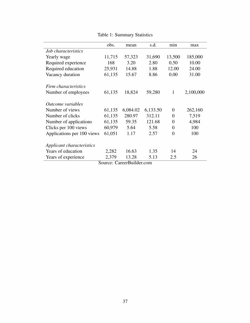
Table 1: Summary Statistics

obs. mean s.d. min maxJob characteristicsYearly wage 11,715 57,323 31,690 13,500 185,000Required experience 168 3.20 2.80 0.50 10.00Required education 25,931 14.88 1.88 12.00 24.00Vacancy duration 61,135 15.67 8.86 0.00 31.00

Firm characteristicsNumber of employees 61,135 18,824 59,280 1 2,100,000

Outcome variablesNumber of views 61,135 6,084.02 6,133.50 0 262,160Number of clicks 61,135 280.97 312.11 0 7,519Number of applications 61,135 59.35 121.68 0 4,984Clicks per 100 views 60,979 5.64 5.58 0 100Applications per 100 views 61,051 1.17 2.57 0 100

Applicant characteristicsYears of education 2,282 16.63 1.35 14 24Years of experience 2,379 13.28 5.13 2.5 26

Source: CareerBuilder.com

37

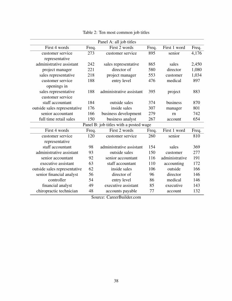
Table 2: Ten most common job titles

Panel A: all job titlesFirst 4 words Freq. First 2 words Freq. First 1 word Freq.

customer service 273 customer service 895 senior 4,176representative

administrative assistant 242 sales representative 865 sales 2,450project manager 221 director of 580 director 1,080

sales representative 218 project manager 553 customer 1,034customer service 188 entry level 476 medical 897

openings insales representative 188 administrative assistant 395 project 883

customer servicestaff accountant 184 outside sales 374 business 870

outside sales representative 176 inside sales 307 manager 801senior accountant 166 business development 279 rn 742

full time retail sales 150 business analyst 267 account 654Panel B: job titles with a posted wage

First 4 words Freq. First 2 words Freq. First 1 word Freq.customer service 120 customer service 260 senior 810

representativestaff accountant 98 administrative assistant 154 sales 369

administrative assistant 93 outside sales 150 customer 277senior accountant 92 senior accountant 116 administrative 191executive assistant 63 staff accountant 110 accounting 172

outside sales representative 62 inside sales 106 outside 166senior financial analyst 56 director of 96 director 146

controller 54 entry level 86 medical 146financial analyst 49 executive assistant 85 executive 143

chiropractic technician 48 accounts payable 77 account 132Source: CareerBuilder.com

38

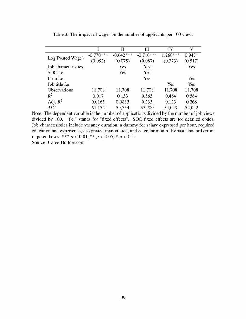
Table 3: The impact of wages on the number of applicants per 100 views

I II III IV V

Log(Posted Wage)-0.770*** -0.642*** -0.710*** 1.268*** 0.947*

(0.052) (0.075) (0.087) (0.373) (0.517)Job characteristics Yes Yes YesSOC f.e. Yes YesFirm f.e. Yes YesJob title f.e. Yes YesObservations 11,708 11,708 11,708 11,708 11,708R2 0.017 0.133 0.363 0.464 0.584Adj. R2 0.0165 0.0835 0.235 0.123 0.268AIC 61,152 59,754 57,200 54,049 52,042

Note: The dependent variable is the number of applications divided by the number of job viewsdivided by 100. "f.e." stands for "fixed effects". SOC fixed effects are for detailed codes.Job characteristics include vacancy duration, a dummy for salary expressed per hour, requirededucation and experience, designated market area, and calendar month. Robust standard errorsin parentheses. *** p < 0.01, ** p < 0.05, * p < 0.1.Source: CareerBuilder.com

39

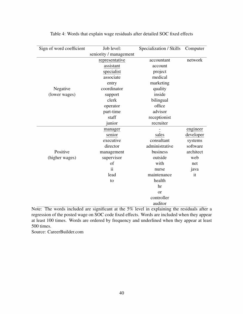
Table 4: Words that explain wage residuals after detailed SOC fixed effects

Sign of word coefficient Job level: Specialization / Skills Computerseniority / management

representative accountant networkassistant accountspecialist projectassociate medical

entry marketingNegative coordinator quality

(lower wages) support insideclerk bilingual

operator officepart-time advisor

staff receptionistjunior recruiter

manager - engineersenior sales developer

executive consultant systemsdirector administrative software

Positive management business architect(higher wages) supervisor outside web

of with netii nurse java

lead maintenance itto health

hror

controllerauditor

Note: The words included are significant at the 5% level in explaining the residuals after aregression of the posted wage on SOC code fixed effects. Words are included when they appearat least 100 times. Words are ordered by frequency and underlined when they appear at least500 times.Source: CareerBuilder.com

40

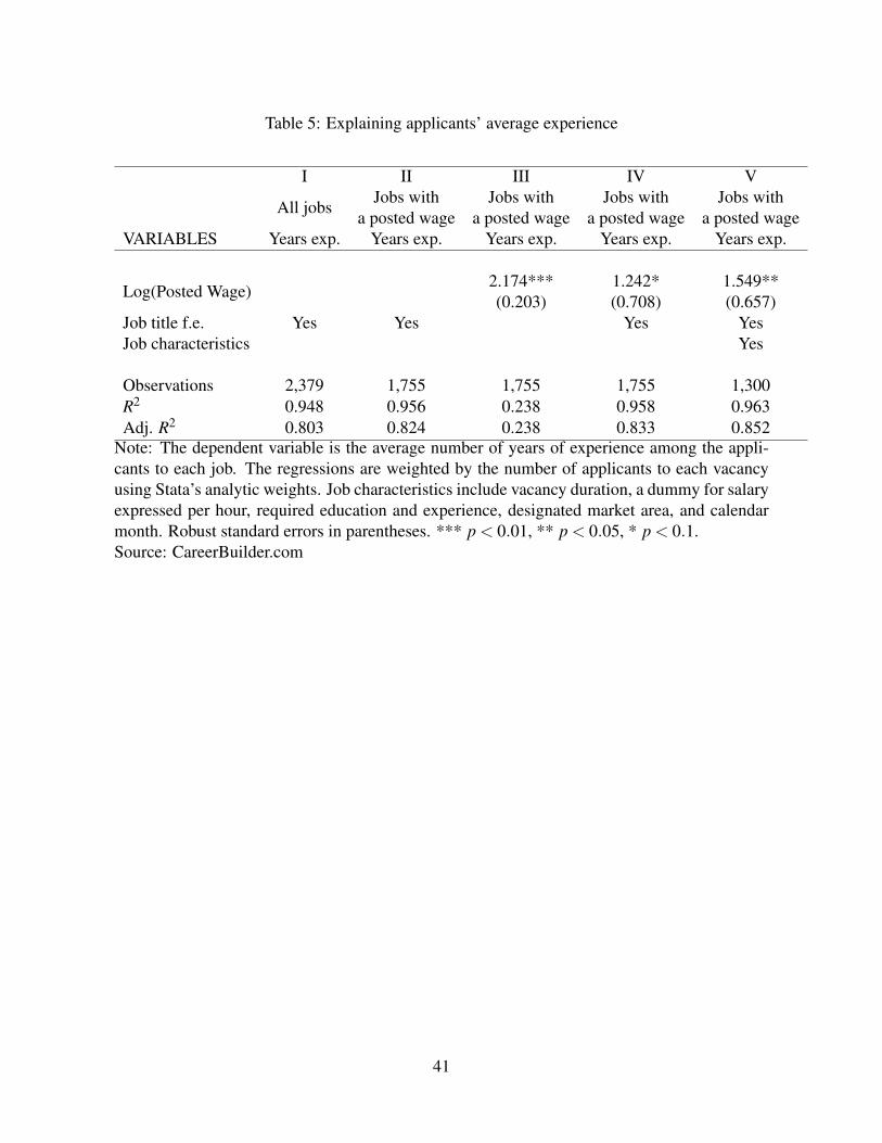
Table 5: Explaining applicants’ average experience

I II III IV V

All jobsJobs with Jobs with Jobs with Jobs with

a posted wage a posted wage a posted wage a posted wageVARIABLES Years exp. Years exp. Years exp. Years exp. Years exp.

Log(Posted Wage)2.174*** 1.242* 1.549**(0.203) (0.708) (0.657)

Job title f.e. Yes Yes Yes YesJob characteristics Yes

Observations 2,379 1,755 1,755 1,755 1,300R2 0.948 0.956 0.238 0.958 0.963Adj. R2 0.803 0.824 0.238 0.833 0.852

Note: The dependent variable is the average number of years of experience among the appli-cants to each job. The regressions are weighted by the number of applicants to each vacancyusing Stata’s analytic weights. Job characteristics include vacancy duration, a dummy for salaryexpressed per hour, required education and experience, designated market area, and calendarmonth. Robust standard errors in parentheses. *** p < 0.01, ** p < 0.05, * p < 0.1.Source: CareerBuilder.com

41

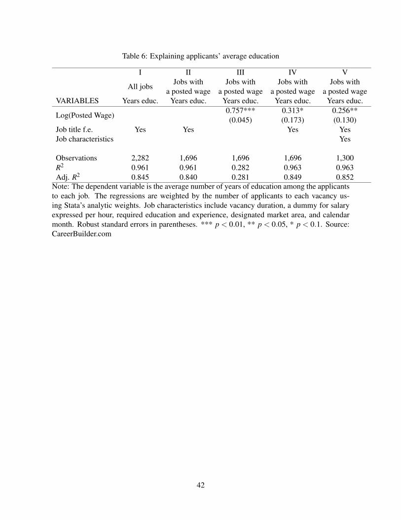
Table 6: Explaining applicants’ average education

I II III IV V

All jobsJobs with Jobs with Jobs with Jobs with

a posted wage a posted wage a posted wage a posted wageVARIABLES Years educ. Years educ. Years educ. Years educ. Years educ.

Log(Posted Wage)0.757*** 0.313* 0.256**(0.045) (0.173) (0.130)

Job title f.e. Yes Yes Yes YesJob characteristics Yes

Observations 2,282 1,696 1,696 1,696 1,300R2 0.961 0.961 0.282 0.963 0.963Adj. R2 0.845 0.840 0.281 0.849 0.852

Note: The dependent variable is the average number of years of education among the applicantsto each job. The regressions are weighted by the number of applicants to each vacancy us-ing Stata’s analytic weights. Job characteristics include vacancy duration, a dummy for salaryexpressed per hour, required education and experience, designated market area, and calendarmonth. Robust standard errors in parentheses. *** p < 0.01, ** p < 0.05, * p < 0.1. Source:CareerBuilder.com

42

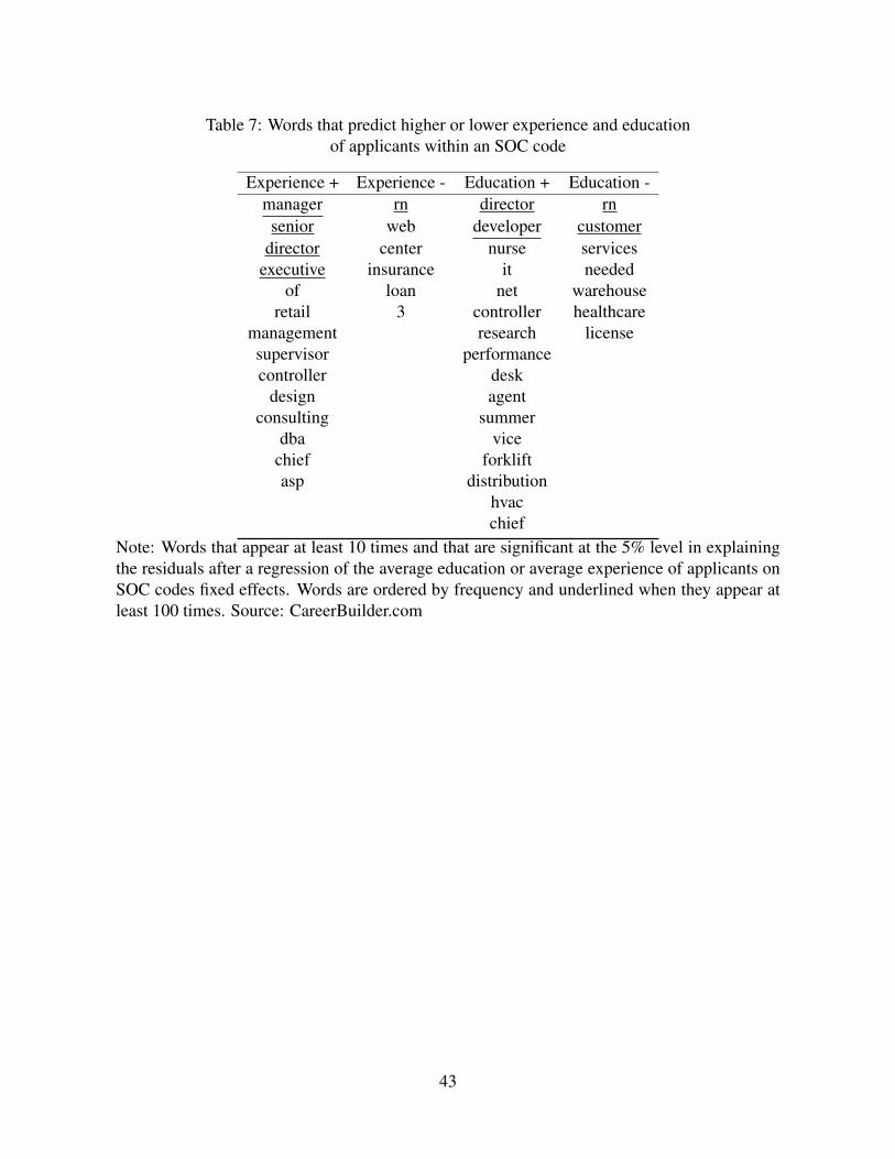
Table 7: Words that predict higher or lower experience and educationof applicants within an SOC code

Experience + Experience - Education + Education -manager rn director rnsenior web developer customer

director center nurse servicesexecutive insurance it needed

of loan net warehouseretail 3 controller healthcare

management research licensesupervisor performancecontroller desk

design agentconsulting summer

dba vicechief forkliftasp distribution

hvacchief

Note: Words that appear at least 10 times and that are significant at the 5% level in explainingthe residuals after a regression of the average education or average experience of applicants onSOC codes fixed effects. Words are ordered by frequency and underlined when they appear atleast 100 times. Source: CareerBuilder.com

43

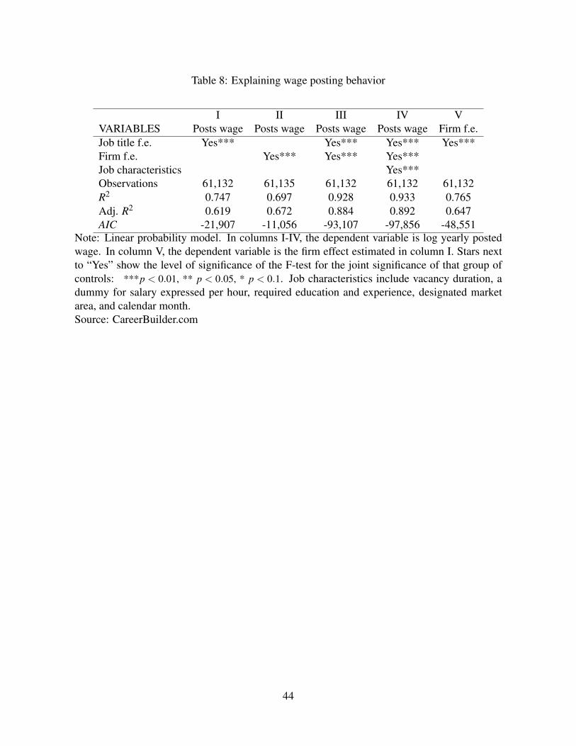
Table 8: Explaining wage posting behavior

I II III IV VVARIABLES Posts wage Posts wage Posts wage Posts wage Firm f.e.Job title f.e. Yes*** Yes*** Yes*** Yes***Firm f.e. Yes*** Yes*** Yes***Job characteristics Yes***Observations 61,132 61,135 61,132 61,132 61,132R2 0.747 0.697 0.928 0.933 0.765Adj. R2 0.619 0.672 0.884 0.892 0.647AIC -21,907 -11,056 -93,107 -97,856 -48,551

Note: Linear probability model. In columns I-IV, the dependent variable is log yearly postedwage. In column V, the dependent variable is the firm effect estimated in column I. Stars nextto “Yes” show the level of significance of the F-test for the joint significance of that group ofcontrols: ***p < 0.01, ** p < 0.05, * p < 0.1. Job characteristics include vacancy duration, adummy for salary expressed per hour, required education and experience, designated marketarea, and calendar month.Source: CareerBuilder.com

44

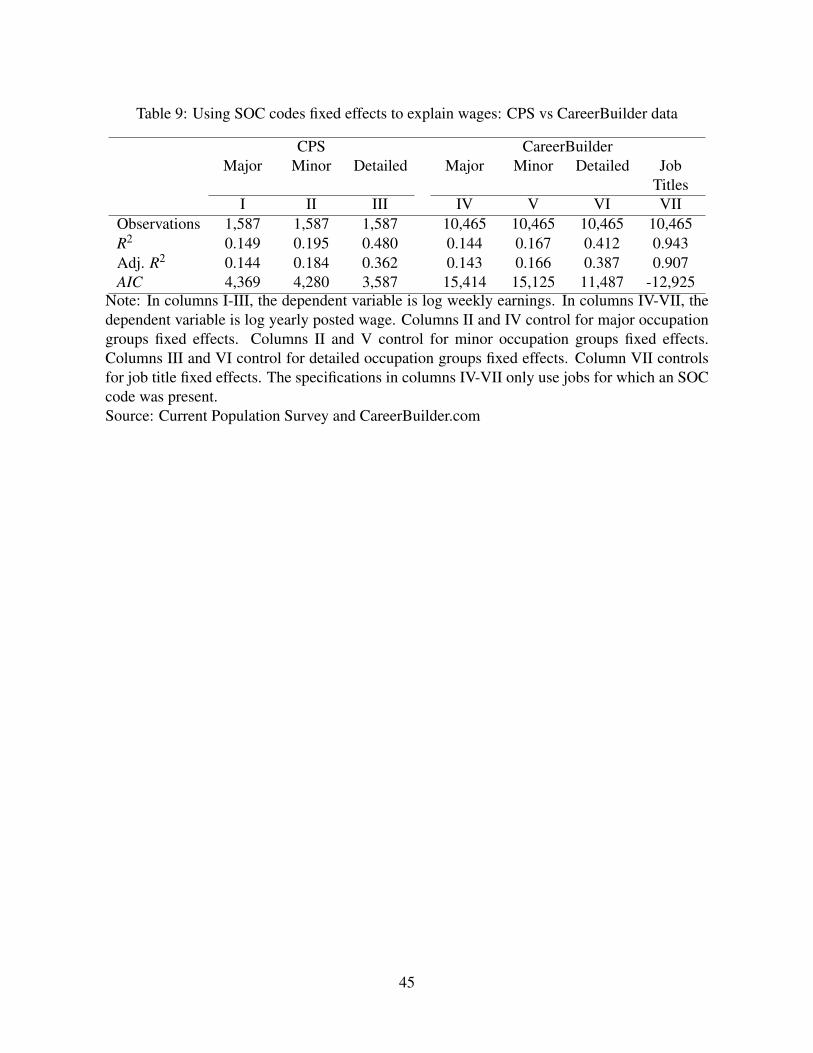
Table 9: Using SOC codes fixed effects to explain wages: CPS vs CareerBuilder data

CPS CareerBuilderMajor Minor Detailed Major Minor Detailed Job

TitlesI II III IV V VI VII

Observations 1,587 1,587 1,587 10,465 10,465 10,465 10,465R2 0.149 0.195 0.480 0.144 0.167 0.412 0.943Adj. R2 0.144 0.184 0.362 0.143 0.166 0.387 0.907AIC 4,369 4,280 3,587 15,414 15,125 11,487 -12,925

Note: In columns I-III, the dependent variable is log weekly earnings. In columns IV-VII, thedependent variable is log yearly posted wage. Columns II and IV control for major occupationgroups fixed effects. Columns II and V control for minor occupation groups fixed effects.Columns III and VI control for detailed occupation groups fixed effects. Column VII controlsfor job title fixed effects. The specifications in columns IV-VII only use jobs for which an SOCcode was present.Source: Current Population Survey and CareerBuilder.com

45

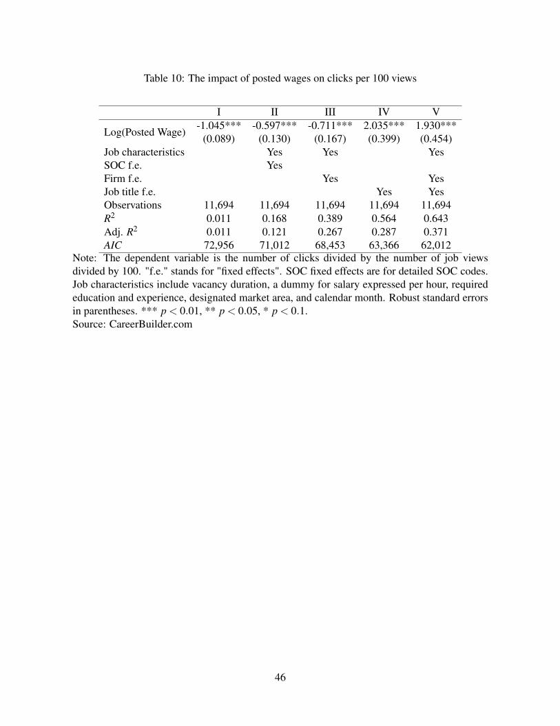
Table 10: The impact of posted wages on clicks per 100 views

I II III IV V

Log(Posted Wage)-1.045*** -0.597*** -0.711*** 2.035*** 1.930***

(0.089) (0.130) (0.167) (0.399) (0.454)Job characteristics Yes Yes YesSOC f.e. YesFirm f.e. Yes YesJob title f.e. Yes YesObservations 11,694 11,694 11,694 11,694 11,694R2 0.011 0.168 0.389 0.564 0.643Adj. R2 0.011 0.121 0.267 0.287 0.371AIC 72,956 71,012 68,453 63,366 62,012

Note: The dependent variable is the number of clicks divided by the number of job viewsdivided by 100. "f.e." stands for "fixed effects". SOC fixed effects are for detailed SOC codes.Job characteristics include vacancy duration, a dummy for salary expressed per hour, requirededucation and experience, designated market area, and calendar month. Robust standard errorsin parentheses. *** p < 0.01, ** p < 0.05, * p < 0.1.Source: CareerBuilder.com

46

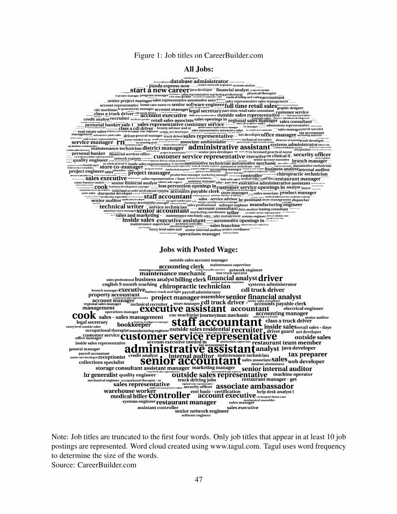
Figure 1: Job titles on CareerBuilder.com

All Jobs:

Jobs with Posted Wage:

Note: Job titles are truncated to the first four words. Only job titles that appear in at least 10 jobpostings are represented. Word cloud created using www.tagul.com. Tagul uses word frequencyto determine the size of the words.Source: CareerBuilder.com

47

Figure 2: Words that predict wages within a given SOC code

Higher Wages:

[0.044;0.060]; [0.077;0.200]; [0.202;1.576] log pointsLower Wages:

[-1.101;-0.169]; [-0.167;-0.104]; [-0.101;-0.063] log points

Note: Words that are significant at the 5% level in explaining the residuals after a regression ofthe posted wage on SOC codes fixed effects (Table B.3, column II) and appear at least 10 times.The big rectangle is "-", which typically separates the main job title from additional details.Word cloud created using www.tagul.com. The size of a word represents its frequency, whilethe color represents the tercile of its coefficient, weighted by frequency.Source: CareerBuilder.com

48

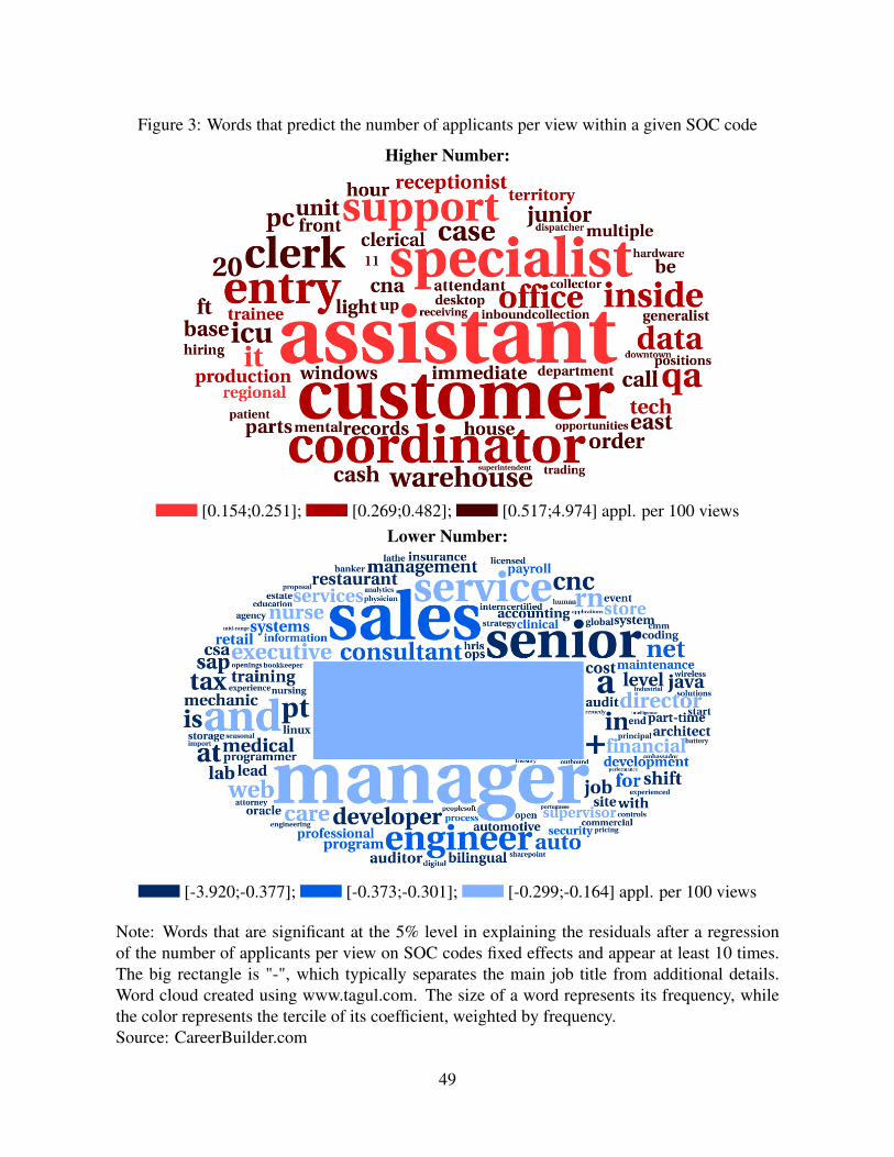
Figure 3: Words that predict the number of applicants per view within a given SOC code

Higher Number:

[0.154;0.251]; [0.269;0.482]; [0.517;4.974] appl. per 100 viewsLower Number:

[-3.920;-0.377]; [-0.373;-0.301]; [-0.299;-0.164] appl. per 100 views

Note: Words that are significant at the 5% level in explaining the residuals after a regressionof the number of applicants per view on SOC codes fixed effects and appear at least 10 times.The big rectangle is "-", which typically separates the main job title from additional details.Word cloud created using www.tagul.com. The size of a word represents its frequency, whilethe color represents the tercile of its coefficient, weighted by frequency.Source: CareerBuilder.com

49

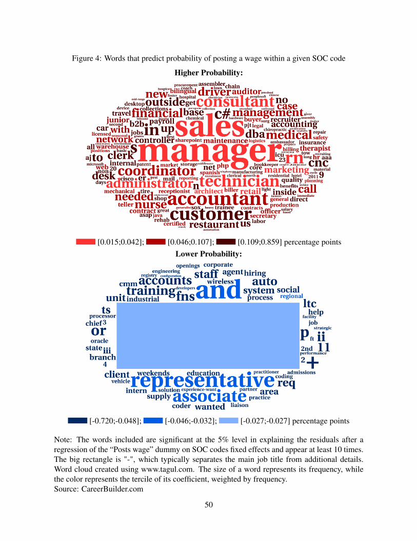
Figure 4: Words that predict probability of posting a wage within a given SOC code

Higher Probability:

[0.015;0.042]; [0.046;0.107]; [0.109;0.859] percentage pointsLower Probability:

[-0.720;-0.048]; [-0.046;-0.032]; [-0.027;-0.027] percentage points

Note: The words included are significant at the 5% level in explaining the residuals after aregression of the “Posts wage” dummy on SOC codes fixed effects and appear at least 10 times.The big rectangle is "-", which typically separates the main job title from additional details.Word cloud created using www.tagul.com. The size of a word represents its frequency, whilethe color represents the tercile of its coefficient, weighted by frequency.Source: CareerBuilder.com

50

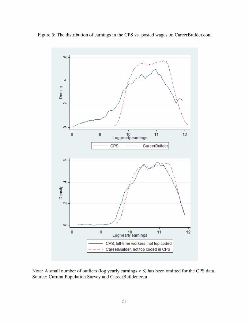
Figure 5: The distribution of earnings in the CPS vs. posted wages on CareerBuilder.com

Note: A small number of outliers (log yearly earnings < 8) has been omitted for the CPS data.Source: Current Population Survey and CareerBuilder.com

51

Appendix A Proofs

Proof of Proposition 1. Using ξ to denote the multiplier on the resource constraint, the first-order conditions of the Lagrangian are

e−λ jky jxk = ξ (11)

for j ∈ {A,B} and k ∈ {L,H}. These four first-order conditions and the resource constrainttogether form a system of five equations with five unknowns (λ jk, ξ ).

Given xL = 1, evaluation of the first-order condition (11) for different values of k yieldsλ jH = λ jL + logxH . Similarly, evaluation of the first-order condition (11) for different valuesof j gives λBL = λAL + logyB− logyA. Substitution of these results into the resource constraintimplies (1).

For this interior allocation to indeed be optimal, we need to verify that the shortest queuelength remains positive. That is, λAL > 0, which by equation (1) is satisfied if and only ifyBxH < yAe2(µ0+µ1).

As mentioned above, efficiency of the equilibrium requires that workers’ expected payoffequals their marginal contribution to surplus, which is equal to ξi. A worker’s expected payoffis the product of his matching probability and the wage that he would be paid. A firm of type( j,k) matches as long as at least one worker applies, which happens with probability 1− e−λ jk .Since there are on average λ jk of such workers applying to the firm, the matching probability ofa worker is

(1− e−λ jk

)/λ jk. Dividing ξ by this matching probabilities yields (2).

Proof of Proposition 2. Using ξi to denote the multiplier on the resource constraint for typei, the first-order conditions of the Lagrangian are

e−λ0Aky0Axk = ξ0 (12)

e−λ1Bky1Bxk = ξ1 (13)

for k ∈ {L,H}. These four first-order conditions and the two resource constraints together forma system of six equations with six unknowns (λ0Ak, λ1Bk, ξ0, ξ1). Given xL = 1, evaluation of theFOCs for the two different values of k yields λ0AH = λ0AL + logxH and λ1BH = λ1BL + logxH .Substituting this into the resource constraints then implies (3) and (4).

As in the proof of proposition 1, we derive the wages by dividing workers’ marginal con-tribution to surplus ξi by their matching probability. Using the same logic as in that proof,the relevant matching probabilities are

(1− e−λ0Ak

)/λ0Ak and

(1− e−λ1Bk

)/λ1Bk. Hence, we

52

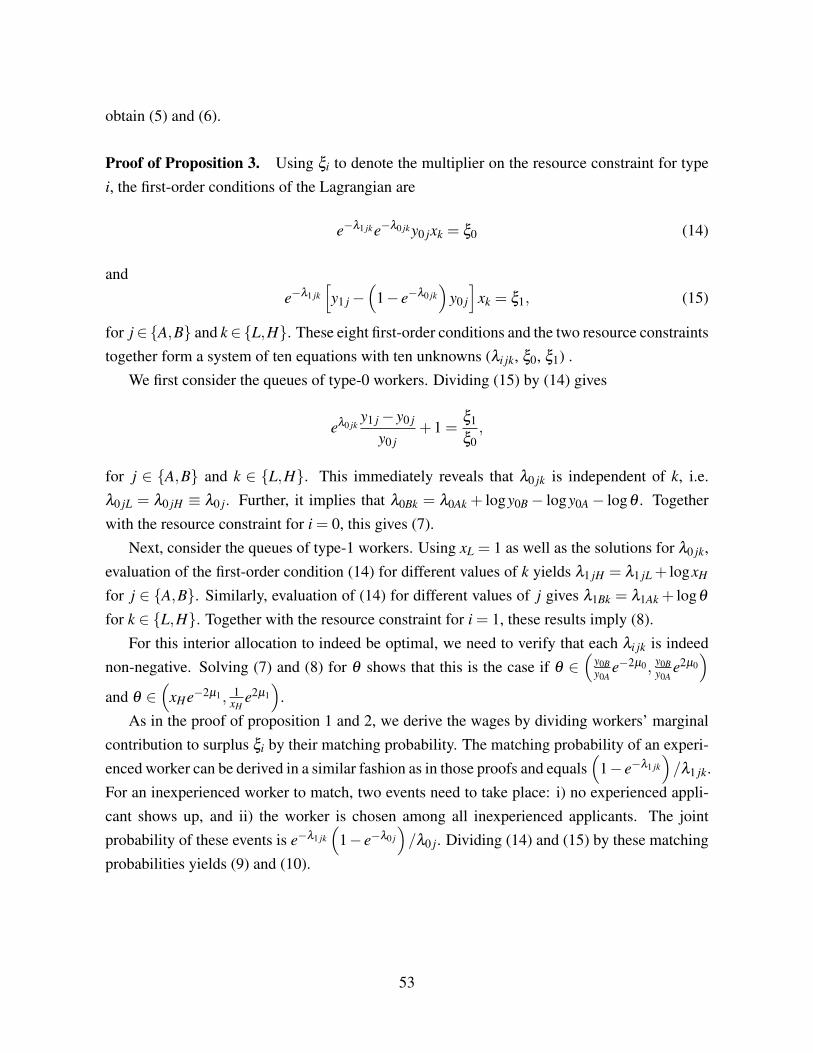
obtain (5) and (6).

Proof of Proposition 3. Using ξi to denote the multiplier on the resource constraint for typei, the first-order conditions of the Lagrangian are

e−λ1 jke−λ0 jky0 jxk = ξ0 (14)

ande−λ1 jk

[y1 j−

(1− e−λ0 jk

)y0 j

]xk = ξ1, (15)

for j∈{A,B} and k∈{L,H}. These eight first-order conditions and the two resource constraintstogether form a system of ten equations with ten unknowns (λi jk, ξ0, ξ1) .

We first consider the queues of type-0 workers. Dividing (15) by (14) gives

eλ0 jky1 j− y0 j

y0 j+1 =

ξ1

ξ0,

for j ∈ {A,B} and k ∈ {L,H}. This immediately reveals that λ0 jk is independent of k, i.e.λ0 jL = λ0 jH ≡ λ0 j. Further, it implies that λ0Bk = λ0Ak + logy0B− logy0A− logθ . Togetherwith the resource constraint for i = 0, this gives (7).

Next, consider the queues of type-1 workers. Using xL = 1 as well as the solutions for λ0 jk,evaluation of the first-order condition (14) for different values of k yields λ1 jH = λ1 jL + logxH

for j ∈ {A,B}. Similarly, evaluation of (14) for different values of j gives λ1Bk = λ1Ak + logθ

for k ∈ {L,H}. Together with the resource constraint for i = 1, these results imply (8).For this interior allocation to indeed be optimal, we need to verify that each λi jk is indeed

non-negative. Solving (7) and (8) for θ shows that this is the case if θ ∈(

y0By0A

e−2µ0, y0By0A

e2µ0

)and θ ∈

(xHe−2µ1 , 1

xHe2µ1

).

As in the proof of proposition 1 and 2, we derive the wages by dividing workers’ marginalcontribution to surplus ξi by their matching probability. The matching probability of an experi-enced worker can be derived in a similar fashion as in those proofs and equals

(1− e−λ1 jk

)/λ1 jk.

For an inexperienced worker to match, two events need to take place: i) no experienced appli-cant shows up, and ii) the worker is chosen among all inexperienced applicants. The jointprobability of these events is e−λ1 jk

(1− e−λ0 j

)/λ0 j. Dividing (14) and (15) by these matching

probabilities yields (9) and (10).

53

Online Appendix

Appendix B Wage Variance Results

The results in Table 9 indicate that job title fixed effects can explain most of the cross-sectionalvariation in wages. A natural concern is that part of this effect is mechanical as our data setcontains many different job titles. In this section, we explore the robustness of the effect in anumber of ways.

First, we perform a permutation test in which we re-estimate the specification with job titlefixed effects (column II) 1000 times with randomly re-assigned wages. The average adjustedR2 is 0 in this case, confirming that our results are not simply the result of the large number ofjob titles.29

Second, we limit the sample to job titles that appear at least two, three or four times. Thisdoes not change the results, as can be seen from Table B.1: even when focusing on job titlesthat appear in at least n ∈ {2,3,4} job postings, we find that job titles explain around 90% ofthe variance in posted wages.

Third, we explore the explanatory power of the first n words of the job title for variousvalues of n. Table B.2 displays the results. The first word of the job title already has a greatdeal of explanatory power: first word fixed effects explain about 60% of the wage variance.Astonishingly, the first word of the job title has greater explanatory power than the most detailedoccupational classification that can be used in the CPS (see Table 9, column VI). Using the firstthree words of the job title significantly improves the explanatory power of the model, with anR2 of 0.93. Using the first four words only slightly improves the explanatory power comparedto using the first three words. Finally, using all words in the job title essentially does not addany explanatory power compared to using the first four words. These results show that the firstfour words of the job title convey almost all of the information that is relevant for posted wages,and justify our choice of using the first four words to define the job title.

Fourth, we explore the explanatory power of a small number of frequent words, i.e. thoselisted in Table 4. In particular, we take the wage residuals after regressing log yearly postedwages on detailed SOC codes fixed effects, and we regress those residuals on fixed effects foreach of the frequent words. The results of this exercise are presented in Table B.3. We findthat the frequent words already explain 22% of the variation in the wage residuals (column III).More than half of this explanatory power is due to the words indicating seniority (column IV),while the remaining explanatory power is roughly equally divided between words indicating

29These results are available upon request.

54

specialties related to computers and other specialties (column V and VI).Fifth, we explore how sensitive the explanatory power of job titles is to the definition of the

wage. Firms often post a wage range rather than a single wage, and we have focused so far onexplaining the midpoint of this range. In Table B.4, we show that job titles are just as powerfulin explaining the minimum of the range (column I) and the maximum of the range (column III).We also find, again, that SOC codes explain less than 40% of the variance in the minimum orthe maximum offered wage (columns II and IV). Finally, we investigate the power of job titlesin explaining how large the wage range is. We define the wage range as the maximum minusthe minimum divided by the midpoint. We divide the range by the midpoint to adjust for thefact that higher wage jobs may also have larger absolute ranges. This range variable takes thevalue of zero when only one wage value is posted. Remarkably, we find that job titles havehigh explanatory power for wage ranges as well: they explain about 80% of the variance in thewage range. By contrast, SOC codes only explain about 20% of the variance in the wage range.We conclude that job titles explain most of the variance in the minimum, the midpoint and themaximum of the posted wage range, as well as in the size of the posted wage range.

55

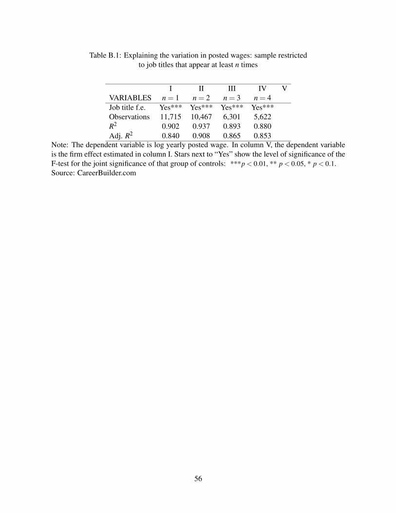
Table B.1: Explaining the variation in posted wages: sample restrictedto job titles that appear at least n times

I II III IV VVARIABLES n = 1 n = 2 n = 3 n = 4Job title f.e. Yes*** Yes*** Yes*** Yes***Observations 11,715 10,467 6,301 5,622R2 0.902 0.937 0.893 0.880Adj. R2 0.840 0.908 0.865 0.853

Note: The dependent variable is log yearly posted wage. In column V, the dependent variableis the firm effect estimated in column I. Stars next to “Yes” show the level of significance of theF-test for the joint significance of that group of controls: ***p < 0.01, ** p < 0.05, * p < 0.1.Source: CareerBuilder.com

56

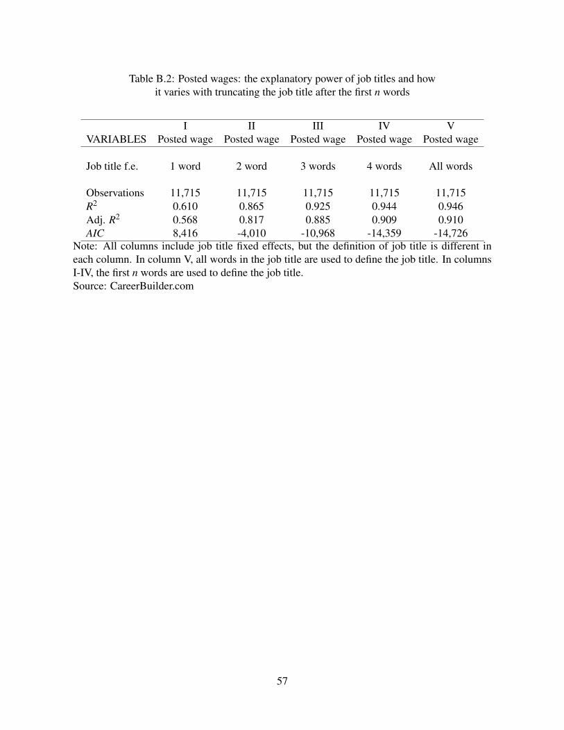
Table B.2: Posted wages: the explanatory power of job titles and howit varies with truncating the job title after the first n words

I II III IV VVARIABLES Posted wage Posted wage Posted wage Posted wage Posted wage

Job title f.e. 1 word 2 word 3 words 4 words All words

Observations 11,715 11,715 11,715 11,715 11,715R2 0.610 0.865 0.925 0.944 0.946Adj. R2 0.568 0.817 0.885 0.909 0.910AIC 8,416 -4,010 -10,968 -14,359 -14,726

Note: All columns include job title fixed effects, but the definition of job title is different ineach column. In column V, all words in the job title are used to define the job title. In columnsI-IV, the first n words are used to define the job title.Source: CareerBuilder.com

57

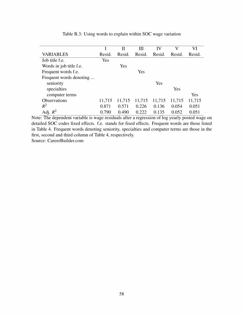
Table B.3: Using words to explain within SOC wage variation

I II III IV V VIVARIABLES Resid. Resid. Resid. Resid. Resid. Resid.Job title f.e. YesWords in job title f.e. YesFrequent words f.e. YesFrequent words denoting ...

seniority Yesspecialties Yescomputer terms Yes

Observations 11,715 11,715 11,715 11,715 11,715 11,715R2 0.871 0.571 0.226 0.136 0.054 0.051Adj. R2 0.790 0.490 0.222 0.135 0.052 0.051

Note: The dependent variable is wage residuals after a regression of log yearly posted wage ondetailed SOC codes fixed effects. f.e. stands for fixed effects. Frequent words are those listedin Table 4. Frequent words denoting seniority, specialties and computer terms are those in thefirst, second and third column of Table 4, respectively.Source: CareerBuilder.com

58

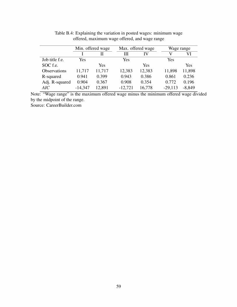
Table B.4: Explaining the variation in posted wages: minimum wageoffered, maximum wage offered, and wage range

Min. offered wage Max. offered wage Wage rangeI II III IV V VI

Job title f.e. Yes Yes YesSOC f.e. Yes Yes YesObservations 11,717 11,717 12,383 12,383 11,898 11,898R-squared 0.941 0.399 0.943 0.386 0.861 0.236Adj. R-squared 0.904 0.367 0.908 0.354 0.772 0.196AIC -14,347 12,891 -12,721 16,778 -29,113 -8,849

Note: “Wage range” is the maximum offered wage minus the minimum offered wage dividedby the midpoint of the range.Source: CareerBuilder.com

59