XVIII IMEKO WORLD CONGRESS Metrology for a Sustainable Development

September, 17 – 22, 2006, Rio de Janeiro, Brazil

OPEN-SOURCE EXCEL TOOLS FOR STATISTICAL METROLOGY FOR THE XVIII IMEKO WORLD CONGRESS

Hung-kung Liu, William F. Guthrie, Juan Soto

NIST, Gaithersburg, MD, USA, liu@nist.gov

Abstract: In this paper we introduce an approach for constructing statistical metrology tools with a Microsoft Excel based interface that uses the open source statistical package R as the computational engine. These metrology tools will enable Excel users to access a larger array of specialized statistical tools for metrology. We will describe our general approach and demonstrate one tool - an automated uncertainty calculator. This uncertainty calculator provides users with a simple and flexible tool for estimating measurement uncertainty using the methods outlined in the ISO Guide to the Expression of Uncertainty in Measurement, popularly known as the ISO GUM. The uncertainty calculator is easy to use for scientists who are comfortable with spreadsheets, can handle a variety of typical correlation structures, and performs a validity check on the results by simulating the coverage probabilities actually attained by the uncertainty intervals. Keywords: statistical metrology, uncertainty, Excel, R.

1. INTRODUCTION

Many scientists use Microsoft Excel1 for data collection and statistical analysis. However, Excel has limited statistical functionality, and may not always work well when used for specialized metrology computations, such as the evaluation of measurement uncertainty. In contrast, the statistical package R [1] is a language and environment for statistical computing and graphics. R provides a wide variety of statistical (linear and nonlinear modeling, classical statistical tests, time-series analysis, classification, clustering, etc.) and graphical techniques, and is highly extensible. The S language developed at Bell Laboratories is often the vehicle of choice for research in statistical methodology, and R provides an open source route to participation in that activity. Thomas Baier's R-(D) COM package and Erich Neuwirth's Excel add-in R-Excel [2,3,4], combined with R, can be used to extend Excel's statistical reach. Using their technology, we have developed scripts that harness the power of R to enable Excel users to use NIST recommended methodologies for statistical

1 Identification of commercial products in this document does not imply recommendation or endorsement by the National Institute of Standards and Technology, nor does it imply that the products identified are necessarily the best available for the purpose.

analysis. One such example is an automatic uncertainty calculator.

Reporting the uncertainty of a measurement result historically has been done using a variety of different approaches. In 1993, however, ISO recommended a standardized approach, in the Guide to the Expression of Uncertainty in Measurement, often called the GUM [5]. The GUM has since been accepted as the default approach among national metrology institutes for assessing and reporting measurement uncertainties. Although adoption of the GUM minimized a wide range of issues that affected uncertainty assessment in the past, computation of measurement uncertainty, especially with correlated variables or correlated uncertainties, remains a problem for many metrologists.

With that in mind, we developed an uncertainty calculator with an Excel-based interface that uses the R as the computational engine to provide scientists and metrologists extended computational capabilities for uncertainty analysis, including symbolic differentiation2, methods for handling correlated input variables, and methods for repeated use of standard uncertainty estimates. The calculator also includes a validity check on the results by simulating the coverage probabilities of the uncertainty intervals obtained. The Kragten spreadsheet [6], and some other uncertainty software tools, do not have these advanced capabilities.

In the remainder of this paper, we discuss the development and use of the uncertainty calculator as an example of the type of tools that we plan to develop as part of a suite of NIST Statistical Metrology Tools. In section 2, we discuss the steps we follow in writing R functions to implement the GUM uncertainty computations. Section 3 describes how the uncertainty spreadsheet fits into the general architecture of our toolkit. Section 4 demonstrates the use of the uncertainty calculator for the calibration of a

2 As explained by Dr. Gordon S. Novak of University of Texas, “A symbolic differentiation program finds the derivative of a given formula with respect to a specified variable, producing a new formula as its output. In general, symbolic mathematics programs manipulate formulas to produce new formulas, rather than performing numeric calculations based on formulas. In a sense, symbolic manipulation programs are more powerful: a formula provides answers to a class of problems, while a numeric answer applies only to a single problem.” (http://www.cs.utexas.edu/users/novak/asg-symdif.html)

load cell and Section 5 outlines the simulation used for the validity assessment of the expanded uncertainty.

2. KEY STEPS IN THE GUM METHOD

One of the key steps incorporated in the GUM is the use of a measurement equation that shows how all the input quantities are combined to obtain the desired measurement result. That is, the value of a measurand θ is related to

input quantities denoted by nµµµ ,,, 21 … 3 through a known functional relationship of the form ( , , , ),1 2f nθ µ µ µ= … (1)

where the function f is generally determined by physical laws relating the relevant quantities. In practice, the values of iµ are not known exactly. However, mean results

nXXX ,, 21 … are available that estimate nµµµ ,,, 21 … , respectively. The GUM recommends the same functional relationship that relates the value θ of the measurand to the input variables nµµµ ,,, 21 … be used to calculate Y

from nXXX ,, 21 … . That is, let Y be the estimate of θ

that is obtained from 1 2,( , , )nY f X X X= … . Consequently

the uncertainty in the measurement result Y must be calculated or estimated by propagating the uncertainties in

the quantities nXXX ,, 21 … used to computeY .

The GUM also recognizes two primary methods, Type A and Type B, for the summarization of the data for each measurement equation input. The most commonly used Type A (or statistical) estimator for the input iµ is the

sample mean of in observations:

1

1.

in

i jj

X Xn =

= ∑ (2)

The most commonly used method for summarizing data to obtain the Type A standard uncertainty of iX is

/i

ix iu S n= where

2( )1

1

i

j i

i

nX X

jSni

−∑==

− (3)

is the sample standard deviation with )1( −= ix ni

ν

degrees of freedom.

Type B (or non-statistical) types of information that can be used to estimate an input include scientific judgment, manufacturer’s specifications, or other indirectly related or incompletely specified information.

3 For economy of notation, GUM uses the same symbol, iX , for the

physical quantity, iµ , and for the random variable, iX , that represents an

estimator of that quantity. We choose not to follow that practice, however, because it complicates the precise description of the mathematical concepts that underpin uncertainty analysis and other statistical analyses.

The GUM procedure for finding the combined standard uncertainty of Y is then to linearize the measurement equation and obtain the standard uncertainty of the linearized result. The first-order Taylor series for values of the function 1( ,..., )nf X X near ),...,( 1 nf µµ is given by

1 ( ,..., )1( ,..., )n f nf X X µ µ≈

11

( ) ... ( )1f fX Xn nX Xn

µ µ ∂ ∂+ − + + − ∂ ∂

(4)

where the quantities in the square brackets are the partial derivatives of the measurement equation with respect to the

ith input to the measurement equation evaluated at iX . Treating the partial derivatives as constants and applying the rules for the propagation of uncertainty of linear measurement equations gives the approximate combined standard uncertainty of 1( ,..., )nf X X

1

222 2

1nc X X

n

f fu u u

X X

∂ ∂≈ + + ∂ ∂ L

1 1

12

,1

2n nX X X X

n

f fu u

X Xρ

∂ ∂+ + ∂ ∂

L (5)

where nXX1

ρ is the correlation between 1X and nX .

Treating the partial derivatives as constants even though they are evaluated at the values of the sample means is not unreasonable because, to the 1st order of approximation, all derivatives are constants. The partial derivatives, called sensitivity coefficients, are typically denoted by xc to

simplify the notation, thus

1 1 1 1 1

2 2 2 2 2 .n n n n nc X X X X X X X X X Xu c u c u c c ρ µ µ≈ + + + +⋅⋅ ⋅L (6)

Finally, to quantify the uncertainty of cu , the GUM suggests computing the effective degrees of freedom of cu using the Welch-Satterthwaite formula

4uY .eff 4 44 4 c uc u

X XX X n n1 1 ...X X1 n

ν

ν ν

=

+ +

(7)

This is only appropriate, however, when all of the individual uncertainties in the denominator are estimated independently of one another.

After obtaining ),...,( 1 nXXf , cu , and effν , probabilistic statements about the measurand

( ,..., ) ( ,..., )1 1 0.95

c

f X X fn nP k ku

µ µ − − ≤ ≤ =

(8)

can be solved using the appropriate constant, k , from Student’s t distribution. Solving for ),...,( 1 nf µµ gives the expanded uncertainty intervals

( ,..., )1 cf X X kun ± (9)

The target coverage probability of these intervals is typically 0.95.

3. TOOL KIT ARCHITECTURE

The suite of NIST Statistical Metrology Tools is constructed using four building blocks: (a) The Microsoft Excel front-end, (b) The Microsoft Excel native programming language, Visual Basic for Applications (VBA), (c) , the open source programming environment for statistical computation and graphics, and (d) R-(D) COM Server V1.35 (R-Excel Add-in) developed by Thomas Baier and Erich Neuwirth. Collectively, these four components are used to build and package computational metrology solutions. Fig. 1 illustrates the use of these different components for uncertainty analysis based on the GUM.

3. The active spreadsheet will load a template that will automatically report a coverage value once all of the data has been entered.

1. Computational metrology solutions are found under the Metrology menu. To execute the GUM, one should select it from the Uncertainty submenu.

2. This will spawn the GUM Uncertainty Analysis window, and request the user to enter a worksheet identifier.

Fig. 1. Computational steps depicting GUM uncertainty analysis using

the R-Excel spreadsheet.

To effectively understand how these components are interrelated we will briefly describe each of these components and how they operate in unison.

Microsoft Excel: Widely available among desktops running Microsoft Windows operating systems, this spreadsheet application enables users to store, process, analyze and graph their data. To provide greater access to alternative statistical methods and libraries, we have opted to: (a) construct tools using both R and R-Excel, and (b) integrate these tools into Excel.

Visual Basic for Applications (VBA): Using VBA subroutines we built up the GUI (graphical user interface) to create a hook for a Metrology menu. Currently, our prototype implementation is based on the GUM. However, we envision that the suite of metrology tools will support additional methods including: the GUM Supplement, Bootstrap uncertainty analysis, Bayes uncertainty analysis, and ANOVA. In addition, we wrote subroutines to replicate the GUM template, thereby enabling users to have multiple worksheets in a single workbook.

R (D) COM Server (R-Excel Add-in): Fortunately, Baier & Neuwirth [4] created a COM server and an Excel

Add-in4 to facilitate the integration of R into Excel. Via this mechanism the client application (e.g., Excel) can communicate with R (the COM server). In fact, there are multiple ways to go about implementing such a connection. However, for our purposes we focused on scratchpad mode5. This mode made sense given the desire to have a solution that would update interactively with each change in a cell value. Additional information regarding COM servers may be found in [2, 4]. An Excel Add-in essentially incorporates a plug-in into the Excel environment, thereby exposing public methods defined in the add-in.

Statistical Computing Environment: Ultimately, data contained in the Excel spreadsheet are passed into R (the statistical computation engine), processed and then returned back to Excel.

4. LOAD CELL CALIBRATION EXAMPLE

We will focus on the calibration and use of a load cell to illustrate the features and operation of the GUM uncertainty spreadsheet. The GUM approach used here will contrast with the presentation of this example in Section 6.1 of the NIST/SEMATECH e-Handbook of Statistical Methods [7], where an approach based on the theory of least-squares regression is used. The GUM approach has the advantages that the computations are carried out in the familiar, standard framework promoted in the GUM [5] and that the computations are largely automated.

Fig. 2 shows the observed deflections of the cell when loaded with the known loads used in the collection of the calibration data. (Note, the loads used here have been scaled relative to the load data presented in [7] to reduce the effects of floating-point errors during computation.) Although it looks like a straight-line model would be an appropriate calibration function, as discussed in [7], a quadratic model is a more appropriate calibration model for this load cell.

0.00

0.50

1.00

1.50

2.00

0 1 2 3

Load, g

Def

lect

ion,

arb

itrar

y un

its

Fig. 2. Load cell calibration data with 20 load levels measured in

duplicate (duplicates not visible on this scale).

4 An Excel Add-in is a software application designed to extend Excel functionality. 5 Writing R Code directly in an Excel worksheet and transferring scalar, vector, and matrix variables between R and Excel.

Denoting the deflection of the cell D for an applied load, L , the quadratic model is expressed 2

1 2 3D L Lβ β β ε= + + + , (10) with unknown parameters iβ and a random measurement error ε . Assuming the random errors are independent and approximately follow a Gaussian distribution with a mean of zero and an unknown standard deviation, σ , the parameters can be estimated using ordinary least-squares regression.

After the fit of the model has been validated using graphical residual analysis and appropriate numerical methods [7], the model can be used to estimate an unknown load applied to the cell based on its observed deflection.

Table 1 gives the output from the fit of the quadratic model to the data.

Table 1. Output from quadratic model fit to load cell data.

Parameter Estimated Value Standard

Uncertainty

1β 6.73566E-04 1.07939E-04

2β 7.32059E-01 1.57817E-04

3β -3.16082E-03 4.86653E-05 σ 2.05177E-04

iν 37

Following [7], suppose an unknown load applied to the

cell produces a deflection of 1.239722D = . Then the observed value of D can be substituted into the calibration function and the load can be obtained by solving for L using the quadratic formula. Thus, in general, the measurement equation to estimate an unknown load using this load cell can be written

( )

3

4

2

22 2 3 1

ˆ ˆ ˆ ˆ DL ˆ

β β β β

β

− + − −= , (11)

where the estimates of each parameter based on the calibration data are differentiated from their actual unknown values by adding a “hat” over the symbol for each parameter. Although there are theoretically two possible solutions for L because we are using a quadratic calibration function, we can easily determine which solution is correct because one solution will fall within (or near) the range of the calibration data and one will be well outside the range of the data. The measurement equation (11) above shows the correct solution for this data.

Of course, for an estimated load value obtained using eq. (11) to have any meaning, an assessment of its uncertainty is also required. Based on the information given in Table 1, it looks like this should only require a fairly straight-forward application of the standard rules for the propagation of uncertainty as outlined in [5]. Although the measurement equation is somewhat complicated, we have estimates and associated standard uncertainties for each of the parameters in the calibration model and the standard uncertainty of an observed deflection is given by, σ̂ , also obtained from the fit of the calibration model.

Unfortunately, however, two complications keep the appropriate uncertainty computations from being as simple

as they might seem at first glance. The first is the fact that the estimated parameter values obtained from the fit of the model are correlated with one another. The second complication arises from the fact that the standard uncertainties of the estimated parameters and the observed deflection are all based on the residual standard deviation of the fit, σ̂ . Thus the uncertainty estimates for each parameter are also (perfectly) correlated with one another. Both of these complications affect the uncertainty computations and must be addressed to ensure that the uncertainty computed for an estimated load will be fit for purpose.

Fortunately these two complications can be overcome fairly easily using the GUM uncertainty spreadsheet since it can be used to account for the correlations between the input variables in the measurement equation and the uncertainty estimates. To take advantage of these features of the spreadsheet, we will need to be able to specify the correlations between the estimated parameters in the calibration output and specify what subset of the standard uncertainties are based on a common estimate. In general, determining the correlations between inputs to a measurement equation can be difficult, however, in this case, because the correlations result purely from the fit of the model to the data, we know what those correlations are [5,8] and they are often included in regression analysis output. For this data, the correlations between the parameter estimates are given in Table 2.

Table 2. Correlations between the parameter estimates.

1β̂ 2β̂ 3β̂

1β̂ 1.000 -0.889 0.781

2β̂ -0.889 1.000 -0.971

3β̂ 0.781 -0.971 1.000

As a further consequence of the mathematics underlying

least-squares fitting, we know that the standard uncertainties of the parameter estimates are all based on the residual standard deviation from the least-squares fit. Because it also seems reasonable to assume that the operation of the load cell is same under regular testing conditions as it is during calibration, it also seems reasonable to estimate the standard uncertainty of the observed deflection, 1.239722D = , using the residual standard deviation, σ̂ .

Fig. 3 shows the layout of the GUM uncertainty spreadsheet. On rows 2, 5, and 8, the user first simply enters the number of inputs in the measurement equation, the names of the inputs, and the measurement equation. The values for the load cell calibration have been entered here based on eq. (11). Then the estimated parameter values, their uncertainties, and degrees of freedom, as obtained from Table 1, are entered in rows 11 through 13 and the columns labeled with the appropriate input name. For each input the user can select whether the standard uncertainty is a Type A or Type B uncertainty in row 14 and can select the appropriate probability distribution for each input in row 15.

In cell A18 the user can select whether or not there are any common uncertainty estimates underlying the standard uncertainties of the inputs. If “Yes” is selected, then the

A B C D E F G H I J K12 4 34 5 beta1 beta2 beta3 D 678910 beta1 beta2 beta3 D11 x i 6.74E-04 7.32E-01 -3.16E-03 1.24E+0012 u i 1.08E-04 1.58E-04 4.87E-05 2.05E-0413 ? i 37 37 37 3714 Type A/B A A A A15 distribution Normal Normal Normal Normal1617 Variable beta1 beta2 beta3 D18 Yes Grouping D D D D19 20 Enter the right triangular correlation matrix:21 Yes beta1 beta2 beta3 D22 beta1 1 -0.888804896 0.781116272 023 beta2 -0.888804896 1 -0.971348202 024 beta3 0.781116272 -0.971348202 1 025 t-factor D 0 0 0 126 y=f(x 1 ,…,x n ) u c (y) ? eff k U(y)27 1.705105569 0.00029227 37 2.026192463 0.00059219528293031 0.94432

Number of input variables:

Input variable names:

Expanded Uncertainty

Are any of the u i 's based on the same uncertainty estimate?

Are any of the estimated input quantities correlated?

Enter your measurement equation below:(-beta2+sqrt(beta2^2-4*beta3*(beta1-D)))/(2*beta3)

Coverage Probability

This coverage probability is the result of a simulation using the estimated input quantities, uncertainties, and other inputs as true values. A simulated coverage near the target value of 95% is an indication of the validity of the uncertainty interval.

Output

Combined Standard Uncertainty

Effective Degrees of Freedom

Coverage Factor =

Fig. 3. Layout of GUM uncertainty spreadsheet.

table shown in columns G through K on rows 17 and 18 is activated and the user can indicate which subsets of standard uncertainties share a common basis. For this example, all of the standard uncertainties are based on the residual standard deviation, so the variables listed in row 17 all share a common class, as denoted by the common value given for each variable in row 18.

As for cell A18, the user can indicate if any of the inputs to the measurement equation are correlated in cell A21. If “Yes” is selected, the symmetric correlation matrix shown in columns G through K and rows 21 through 25 is activated. The user can then enter the correlations in the upper right triangle of the correlation matrix, which is shaded on the spreadsheet. The lower triangle of the matrix is filled in automatically based on its symmetry.

Once all of the necessary inputs have been entered, the results are computed and displayed in the table in columns A through E and rows 23 through 32. For this example, we can see that an estimated load of 1.705106L = g is associated with the observed deflection of 1.239722D = (the number of significant digits given here matches [7]). The estimated load has a combined standard uncertainty of -42.9227 10cu = × g with 37 degrees of freedom. The expanded uncertainty, computed using a coverage factor of about 2.026k = obtained from Student’s t distribution, is -45.92 10U = × g. Finally the value given in cell E31 shows the estimated long-run coverage probability of this type of expanded uncertainty interval. The fact that a value near nominally-desired coverage of 95 % was attained indicates that the approximations used in the GUM should work well in this application. Had the

coverage probability been much lower or higher than 95 % that would indicate that other methods for uncertainty assessment should probably be considered.

To the number of digits reported, these values are quite close to the results given in [7], illustrating the similarity of these two approaches. For further comparison, if the correlations between the inputs and the uncertainty estimates had not been taken into account, the expanded uncertainty would have been -410.51 10U = × g, almost twice the level of the appropriate value, clearly demonstrating the potential impact correlations can have in uncertainty assessment.

5. VALIDITY OF UNCERTAINTY INTERVALS

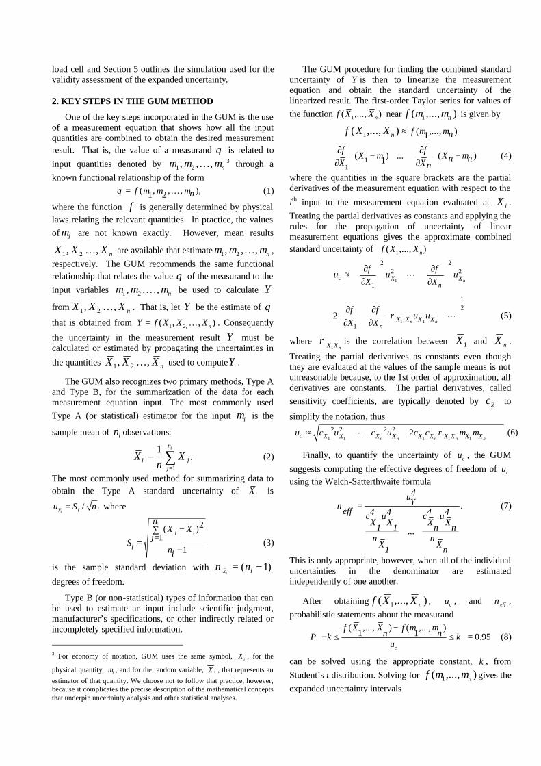
As described in section 2, the GUM takes ( , ( ), ( ))i i iX u X Xν , for i 1,...,n,= as its input to produce an uncertainty interval I. The true unknown frequentist coverage probability 1 nP( f ( ,..., ) I )µ µ ∈ (12) measures the validity of the GUM procedure6. The unknown coverage probability can be estimated by the coverage frequency based on a Monte Carlo study of a large number of N replicates. We study the validity of the GUM uncertainty interval by checking how close this coverage frequency is to its target of 0.95.

In the Monte Carlo study, we use the estimated quantities ( , ( ), ( ))i i iX u X Xν and the user-provided

6 This assessment of the validity is based on the assumption that the values observed for each input quantity are sufficiently near their associated true values, as described below, so that the simulation results based on the input estimates will be relevant to the physical situation.

correlation matrix as the true values to

simulate ))(),(,( ∗∗∗iii XXuX ν . In other words, we use

iX as iµ , and generate new values of iX based on the new artificially known measurand. We denote the simulated iX as *

iX . We apply the GUM approach to

the simulated data ( , ( ), ( ))i i iX u X Xν∗ ∗ ∗ , for i 1,...,n,= to

obtain an uncertainty interval ∗I . This process is repeated N times to yield N such ∗I ’s. The coverage probability is then estimated by the relative frequency of

the coverage of ),...,( 1 nXXf by these N intervals.

)(),...,(

)(),...,(

,...,

**1

**1

**1

n

n

n

XX

XuXu

XX

νν

GUM *I

∈

= otherwise 0,

),...,( if ,1 *1 IXXf

Countn

1

N2

Fig. 4. Schematic depiction of the simulation process.

Fig. 4 illustrates this simulation process. The coverage

frequency equals∑ NCount / .

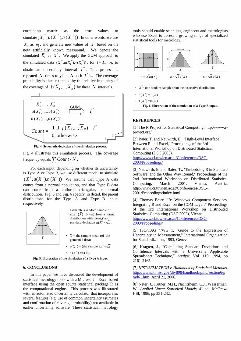
For each input, depending on whether its uncertainty is Type A or Type B, we use different model to simulate

))(),(,( ∗∗∗ XXuX ν . We assume that Type A data comes from a normal population, and that Type B data can come from a uniform, triangular, or normal distribution. Fig. 5 and Fig. 6 specify, in detail, the parent distributions for the Type A and Type B inputs respectively.

Generate a random sample of size from a normal distribution with mean and standard deviation .

• = the sample mean (of the generated data)

• u( ) = (the sample s.d.) /

•

X

2S

( ) ( )X Xν ν∗ =

( ) 1( )X nν + =X

( )u X n×

nX ∗

X ∗

Fig. 5. Illustration of the simulation of a Type A input.

6. CONCLUSIONS

In this paper we have discussed the development of statistical metrology tools with a Microsoft Excel based interface using the open source statistical package R as the computational engine. This process was illustrated with an automated uncertainty calculator that incorporates several features (e.g. use of common uncertainty estimates and confirmation of coverage probability) not available in earlier uncertainty software. These statistical metrology

tools should enable scientists, engineers and metrologists who use Excel to access a growing range of specialized statistical tools for metrology.

• = one random sample from the respective distribution

•

•

X ∗

( ) ( )u X u X∗ =

( ) ( )X Xν ν∗ =

X

2S

1/a

2a(= ± a)

X

1/2a2a (= ± a)

X

a = 3 ( )u X a = 6 ( )u X s = n ( )u X

Fig. 6. Illustration of the simulation of a Type B input.

REFERENCES

[1] The R Project for Statistical Computing, http://www.r-project.org/

[2] Baier, T. and Neuwirth, E., "High-Level Interface Between R and Excel,'' Proceedings of the 3rd International Workshop on Distributed Statistical Computing (DSC 2003). http://www.ci.tuwien.ac.at/Conferences/DSC-2003/Proceedings/

[3] Neuwirth, E. and Baier, T., "Embedding R in Standard Software, and the Other Way Round,'' Proceedings of the 2nd International Workshop on Distributed Statistical Computing, March 2001, Vienna, Austria. http://www.ci.tuwien.ac.at/Conferences/DSC-2001/Proceedings/index.html

[4] Thomas Baier, “R: Windows Component Services, Integrating R and Excel on the COM Layer,” Proceedings of the 3rd International Workshop on Distributed Statistical Computing (DSC 2003), Vienna. http://www.ci.tuwien.ac.at/Conferences/DSC-2003/Proceedings/

[5] ISO/TAG 4/WG 1, "Guide to the Expression of Uncertainty in Measurement," International Organization for Standardization, 1993, Geneva.

[6] Kragten, J., “Calculating Standard Deviations and Confidence Intervals with a Universally Applicable Spreadsheet Technique,” Analyst, Vol. 119, 1994, pp 2161-2165.

[7] NIST/SEMATECH e-Handbook of Statistical Methods, http://www.itl.nist.gov/div898/handbook/pmd/section6/pmd61.htm, April 21, 2006.

[8] Neter, J., Kutner, M.H., Nachtsheim, C.J., Wasserman, W., Applied Linear Statistical Models, 4th ed., McGraw-Hill, 1996, pp 231-232.