OPEN PIT PRODUCTION SCHEDULING APPLYING

META HEURISTIC APPROACH

A THESIS SUBMITTED IN PARTIAL FULFILLMENT OF THE

REQUIREMENT FOR THE DEGREE OF

Bachelor of Technology

In

Mining Engineering

By

BITANSHU DAS

108MN044

DEPARTMENT OF MINING ENGINEERING

NATIONAL INSTITUTE OF TECHNOLOGY

ROURKELA-769008

2011-2012

i

OPEN PIT PRODUCTION SCHEDULING APPLYING

META HEURISTIC APPROACH

A THESIS SUBMITTED IN PARTIAL FULFILLMENT OF THE

REQUIREMENT FOR THE DEGREE OF

Bachelor of Technology

In

Mining Engineering

By

BITANSHU DAS

108MN044

Under the Guidance of

Dr. S. Chatterjee

Assistant Professor

DEPARTMENT OF MINING ENGINEERING

NATIONAL INSTITUTE OF TECHNOLOGY

ROURKELA-769008

2011-2012

ii

National Institute of Technology

Rourkela

CERTIFICATE

This is to certify that the thesis entitled “Open Pit Production Scheduling applying Meta

Heuristic approach” submitted by Sri Bitanshu Das (Roll No. 108MN044) in partial fulfillment

of the requirements for the award of Bachelor of Technology degree in Mining Engineering at

the National institute of Technology, Rourkela is an authentic work carried out by him under my

supervision and guidance.

To the best of my knowledge, the matter embodied in this thesis has not formed the basis for the

award of any Degree or Diploma or similar title of any university or institution.

Date: Dr. S. Chatterjee.

Assistant Professor

Deptt. of Mining Engg

NIT, Rourkela -769008

iii

ACKNOWLEDGEMENT

I take the opportunity to express my deep reverence and gratitude to my supervisor Prof. S.

Chatterjee for his inspiring guidance, help, constructive criticism and valuable suggestions

during the course of the work. I find words inadequate to thank him for his encouragement and

effort in improving my understanding of this project.

I am also grateful to all faculty members and staff of Mining Department, NIT Rourkela who

have helped me during the course.

Last but not the least, my sincere thanks to all my well-wishers and friends who have patiently

extended all sorts of help for accomplishing this dissertation.

Date: (Bitanshu Das)

Roll No. – 108MN044

Department of Mining Engineering

Rourkela - 769008

iv

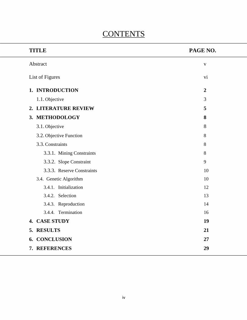
CONTENTS

TITLE PAGE NO.

Abstract v

List of Figures vi

1. INTRODUCTION 2

1.1. Objective 3

2. LITERATURE REVIEW 5

3. METHODOLOGY 8

3.1. Objective 8

3.2. Objective Function 8

3.3. Constraints 8

3.3.1. Mining Constraints 8

3.3.2. Slope Constraint 9

3.3.3. Reserve Constraints 10

3.4. Genetic Algorithm 10

3.4.1. Initialization 12

3.4.2. Selection 13

3.4.3. Reproduction 14

3.4.4. Termination 16

4. CASE STUDY 19

5. RESULTS 21

6. CONCLUSION 27

7. REFERENCES 29

v

ABSTRACT

Production scheduling of a mine is required for effective and economic operations of a mine.

Here we are trying to perform production scheduling of mining of mineral blocks under some

specific constraints to maximize the profit. The large number of variables and inequalities

involved in the process makes it nearly impossible to solve using classical optimization

techniques. The techniques and softwares available take a huge amount of time to produce

optimized solutions. In this project Genetic Algorithm, a metaheuristic algorithm, has been

considered to perform the optimization. The solution provided may not be optimized but will

be very nearly optimized and will take significantly lesser time. It starts from a random

solution performing several crossovers, mutations and eliminations to reach the optimized

solution. A study was carried out in an open pit iron ore mine. The NPV of the mine was

found to be a cumulative of over 551 million $. The average stripping ratio was calculated to

be 1.72 over the period of 4 years. The computational time required to solve the problem was

31 mins.

vi

List Of Figures:

Fig. No. Fig. Title Page No.

3.1 Ore body having 9 mineral blocks 9

3.2 Different components of GA 11

3.3 Ore body with 9 blocks 12

3.4 Sample 27-bit chromosome 13

3.5 Roulette wheel selection 14

3.6 Two sample chromosome having highest probability

of selection 14

3.7 Crossover operation in two parent chromosomes 15

3.8 Mutation operation to produce new chromosome 16

3.9 Flowchart for working principles of GA 17

5.1 Tonnage extracted per year graph 21

5.2 3D view of the ultimate pit 22

5.3 Ultimate Pit in Y-Z axis 22

5.4 The bar graph of DCF for each individual year 23

5.5 The cumulative line graph of NPV for the mine 24

5.6 The Stripping Ratio for each Year 24

1

CHAPTER 1

INTRODUCTION

OBJECTIVE

2

1. INTRODUCTION

Mine production scheduling is an optimization process which assigns the extraction sequence of

a mining block under certain constraints such that it maximizes the net profit. Traditionally,

interpolation techniques such as kriging, from the drillhole sample data , is used to build a block

model of the ore body for open pit mine planning and design. This single model is assumed to be

a fair representation of reality and is used for mine design and optimisation. The design process

consists of 3 main steps: (a) finding the block extraction sequence which produces the best net

present value (NPV) whilst satisfying the geotechnical slope constraints, and (b) optimising the

mining schedule and cut off grades (COG). The NPV of this “optimal” schedule is considered as

a main criterion of the economic viability of the project.

The mine production scheduling problems are difficult to solve with commercial solvers. They

are large scale mixed integer programming problem having very large dimensions of search

space and imposed constraints equations. Solving such problems using classical search

algorithms and optimization methods are very difficult and time taking. However there are

approaches using which these types of problems can be solved using approximation. In open pit

mine planning and production scheduling, Lerchs-Grossmann algorithm combining with

heuristic approach is industry standard, although network flow algorithm are also efficient and

are well suited. Traditionally mining schedule can be generated by a three step process. First, by

implementing the Lerchs-Grossman (L-G) algorithm1 (Whittle 1999) the ultimate pit is obtained.

In the second step, the ultimate pit is sub-divided into a series of nested pits, or pushbacks by a

different parameterization algorithm, (Seymour 1995). Lastly, an Mixed Integer Program (MIP),

or heuristic algorithm, is applied on the series of small pits to obtain the production scheduling

(Ramazan and Dimitrakopoulos 2007). The large mine scheduling problem can also be solved by

the aggregation of blocks to reduce the number of integer variables (Boland et al. 2009). Though

the algorithm provides an optimal solution, it has two major limitations. First, for scheduling a

large size deposit, the aggregation approach is also impossible to solve with presently available

commercial solvers. Secondly, changing the economic values of the blocks by aggregation,

ultimately changes the entire problem into something far different from the original problem.

3

Various non-traditional methods such as simulated annealing (Albor and Dimitrakopoulos,

2009), genetic algorithms (Pendharkar and Rodger, 2000), tabu search (Lamghari and

Dimitrakopoulos 2010) have been applied for solving large scale MIP problems. Metaheuristic

algorithm is the method in which a random solution is iteratively improved to reach towards

optimization under specific constraints. Metaheuristics make few or no assumptions about the

problem being optimized and can search very large spaces of candidate solutions (Goldberg,

1989). Metaheuristics do not guarantee that the solution will be optimized but the obtained

solution will be very near to the optimal solution in a significantly less computational time

(Glover and Kochenberger, 2003). Although, these algorithms have shown significantly

improved results in terms of computational time, however, generating the random solutions

which satisfy the slope constraints is a cumbersome process.

Though, the computational time in genetic algorithm is significantly less but the main problem

associated is to generate the initial chromosomes satisfying the constraints of the problem. In this

thesis, all the constrained equations of the optimization problem have been incorporated in the

objective function and then the problem has been solved as an unconstrained problem as

producing random initial solutions is easier.

Objective

The objectives of this thesis are the following:

• To create an algorithm that will incorporate the constraints in the objective function and

process the data to provide solution in a significantly less time compared to the available

techniques.

• To calculate the ultimate pit, net present value (NPV) and stripping ratio of the mine from

the generated optimal solution

4

CHAPTER 2

LITERATURE REVIEW

5

2. LITERATURE REVIEW

The ideal criteria for production scheduling should be maximization of the net present value

(NPV) of the pit, but still after four decades of continuing efforts and research, this goal could

not be achieved. The pit outline with the highest value cannot be determined until the block

values are known. The block values are not known until the mining sequence is determined; and

the mining sequence cannot be determined unless the pit outline is available (Whittle, 1999)

Various approaches for production scheduling optimization have been tried. The efforts vary

from simulation studies (Pana, 1965), linear and integer programming studies (Barbaro and

Ramani, 1986), to dynamic programming (Mukherjee, 1994). Linear programming (LP) and

integer programming (IP) approaches have received greater attention among the different

methods adopted as applied to production scheduling. But the computational time for these

techniques generally increases as the number of constraints increase. Dynamic programming

models also limitations in terms of the total number of state variables. These models were

unsuitable for real-life situations because only a limited number of possible states (production

rates) can be examined at a time. Fuzzy linear programming (Pendharkar, 1997) approach was

used to allow for setting fuzzy priorities in the linear programming model. These fuzzy priorities

allow for deviations in quality without compromising on overall customer and company

satisfaction. In simulation approaches, the optimality of the solution is not guaranteed along with

the high overhead in terms of computational time (Pana 1965) making it unpopular for study for

production scheduling. Traditional optimization methods like gradient search and local exchange

show poor performance (in terms of computer time) in large-scale. Non linear programming

(NLP) considers factors like “economies of scale” and “economies of scope” etc which are ignored by

linear programming (LP) which considers unit cost independent of the volume of production (economies

of scale) and hence giving NLP advantage over LP. The cost estimates in NLP are nonlinear and

dependent of the production volume. The NLP problems have varying optimization algorithms depending

in problems as no single optimization algorithm works for all NLP problems. The type of objective

function and the constraint should be known for selecting an algorithm for solving an NLP problem,

(Hiller and Lieberman, 1995) .

6

Several nontraditional approaches like simulated annealing (SA) algorithms (Albor and

Dimitrakopoulos, 2009), the tabu search (TS) (Lamghari and Dimitrakopoulos 2010), and Genetic

Algorithms (GA) (Pendharkar and Rodger, 2000) which are based on random, genetic, and

neighborhood have been proposed to solve complex, nonlinear optimization problems. Complex,

nonlinear problems with several local optima can be solved efficiently by heuristic approaches. Heuristic

approaches or hybrids of heuristic-traditional approaches have been proved better than traditional,

gradient-based optimization approaches in solving optimization problems with several local optima

Genetic Algorithms are useful for optimization problems with complex search spaces and when

the convexity of the objective function is not necessary. Traditional gradient-based optimization

methods simulated annealing and tabu search algorithms rely on how close the solutions are to

each other. They may either converge to local optimum or take a long time to converge to global

optimum (De Jong., 1998). GA, when compared to SA and TS, will necessarily be a better

optimization approach when computational time is short and in case of large NP-hard

combinatorial problems and complex engineering problems in the continuous domain (Reeves,

1997). But if longer computational time is permitted then TS and SA may outperform GA. The

selection of GA parameters, such as the mutation rate, crossover, and population size and

sampling of the initial set of population members affects the performance of a GA in a given

search space. Ali et al. (2009) applied genetic algorithm in solving linear equation systems. The

Genetic Algorithm (GA), a meta heuristic approach, has great advantage for efficient feature

selection which provides close to optimum feature subset with a reasonable amount of time

(Hong and Cho, 2006).

7

CHAPTER 3

METHODOLGY

OBJECTIVE FUNCTION

CONSTRAINTS

GENETIC ALGORITHM

8

3. METHODOLOGY

When solving a mine production scheduling problem, first of all the objective function is

formulated i.e. the problem is expressed in the form of a mathematical equation. Then the

constraints of the problem are expressed as mathematical equation. In this thesis, the production

scheduling problem was solved by incorporating the constraint equations in the objective

function to make it easier to generate the initial random pool of solution. After the introduction

of the constraint equations in the objective function and imposing the penalizing constants the

modified objective function is obtained.

3.1 Objective Function

In general, production scheduling problem can be defined in the form of the following

mathematical equation:

max f(x)= (3.1)

where xi,t is the ith

block extracted at time t

Ci is the Block Economic Value of the xi,t block

i=1,2,3,….,N is the number of block

t=1,2,3,…,T is the number of year

r is the annual rate of interest

3.2 Constraints

3.2.1. Mining Constraints:

Every mine has an extraction constraint. Because of the mining machinery available,

it cannot extract beyond a certain tonnage. The following equation shows that the

mine on which the study was carried out cannot extract more than D tons of material

9

(3.2)

Where ai is the tonnage of ith

block.

Similarly, if a mine extracts below a certain amount of tonnage of material, the

machines are likely to remain idle. This is also an unfavorable condition and hence to

avoid it, mine production should be more than E tons of material expressed by the

following equation

(3.3)

Where di is the tonnage of ith

block

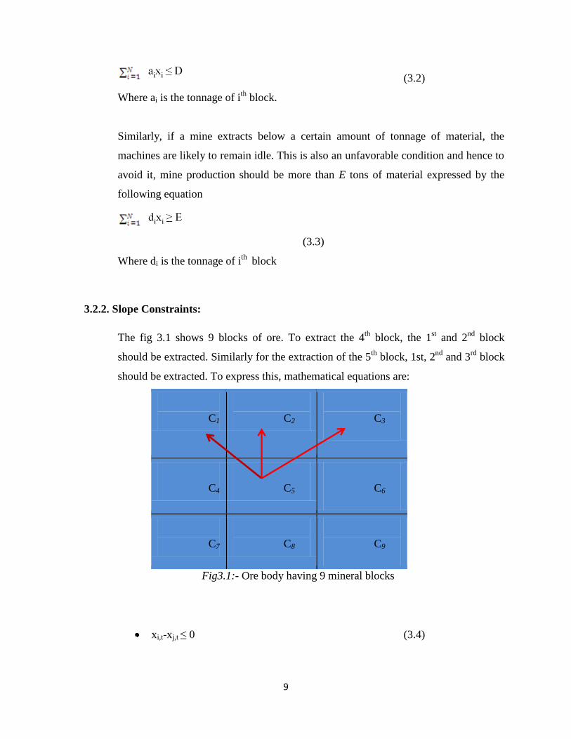
3.2.2. Slope Constraints:

The fig 3.1 shows 9 blocks of ore. To extract the 4th

block, the 1st and 2

nd block

should be extracted. Similarly for the extraction of the 5th

block, 1st, 2nd

and 3rd

block

should be extracted. To express this, mathematical equations are:

C1

C2

C3

C4

C5

C6

C7

C8

C9

Fig3.1:- Ore body having 9 mineral blocks

xi,t-xj,t ≤ 0 (3.4)

10

3.3.2 Reserve Constraints:

A block is either extracted or it hasn’t been extracted. For this, the value 0 is taken for

x if the block has been extracted and the value 1 is taken if the block hasn’t been

extracted.

(3.5)

Modified Objective Function

In constrained GA, producing random initial set of solutions is a cumbersome task. So, an

approach is followed to introduce the constraint equations in the objective functions using

penalizing constants to make the problem an unconstrained and hence producing random initial

set of solutions is easier.

After introducing the constraint equations in the objective function, the modified objective

function is

(3.6)

Where, µ1, µ2, µ3 and µ4 are penalizing constants having very large positive values so that when

constraints are violated, the chromosome gets rejected during selection process.

3.4 GENETIC ALGORITHM

The Genetic Algorithm (GA) is a parallel search technique that begins with a set of possible

solutions as a population. Each possible solution (population member) is evaluated for its fitness.

The fitness of a population member is calculated using the objective function. High-fitness

population members include solutions that possess either a higher objective function value (in

11

case of maximization) or a lower objective function value (in case of minimization problem);

therefore, the fitness of the promising population member is either directly proportional to the

objective function value (in case of maximization problems) or inversely proportional to the

objective function value (in case of minimization problems). The initial population is created by

generating random population members. After evaluating the fitness of each population member,

a subsequent generation of population is generated by applying genetic operators, such as

selection, crossover, and mutation, to individuals in the current population (Pendharkar and

Rodger, 2000). The selection crossover and mutation operators are designed in such a way that,

from one generation of population to another, the average fitness of the population generally

increases. The best fitness member of any generation is the solution to the optimization problem

(De Jong, 1988). GAs mimic some of the processes observed in natural selection through the

Darwinian notion of “survival of the fittest”.

Fig3.2:- Diagram showing different components of GA

Unlike classical techniques, the algorithm works with a population of possible solutions rather

than a single solution. The algorithm terminates when either a maximum number of iterations

have been performed, or an optimal solution with satisfactory fitness level has been reached for

the population. If the algorithm has terminated due to a maximum number of iterations, a

satisfactory solution may or may not have been reached (Goldberg, 1989).

Genetic algorithms are applicable in various fields like bioinformatics, computational science,

engineering, economics, chemistry, manufacturing, mathematics, physics, etc.

A typical genetic algorithm requires:

a genetic representation of the solution domain,

a fitness function to evaluate the solution domain.

The solution is represented as an array of bits. The parts of the bits can be aligned easily because

they have a fixed size facilitating simple crossover operations. Due to this property, these

12

genetic representations are convenient. In case of variable length representations, crossover

implementation is more complex. In genetic programming, tree-like representations are used

whereas the graph-form representations are used in evolutionary programming.

The quality of the represented solution is determined by the fitness function defined, which is

always dependent on the problem. In cases where it is hard or even impossible to define the

fitness function, interactive genetic algorithm is used.

Once the genetic representation and the fitness function are defined, a GA proceeds to initialize a

population of solutions (usually randomly) and then to improve it through repetitive application

of the mutation, crossover, inversion and selection operators (Deb, 2010) as shown in fig 3.2.

3.4.1 Initialization

Initially a random pool of solution is generated to form an initial population. The size of the pool

of solution may range from hundreds to thousands or more depending on the nature of the

problem. To allow an entire range of possible solution (search space), the initial population is

generated randomly. But sometimes the solutions maybe “seeded” in areas where there are more

chances of the existence of optimal solutions (Deb, 2010).

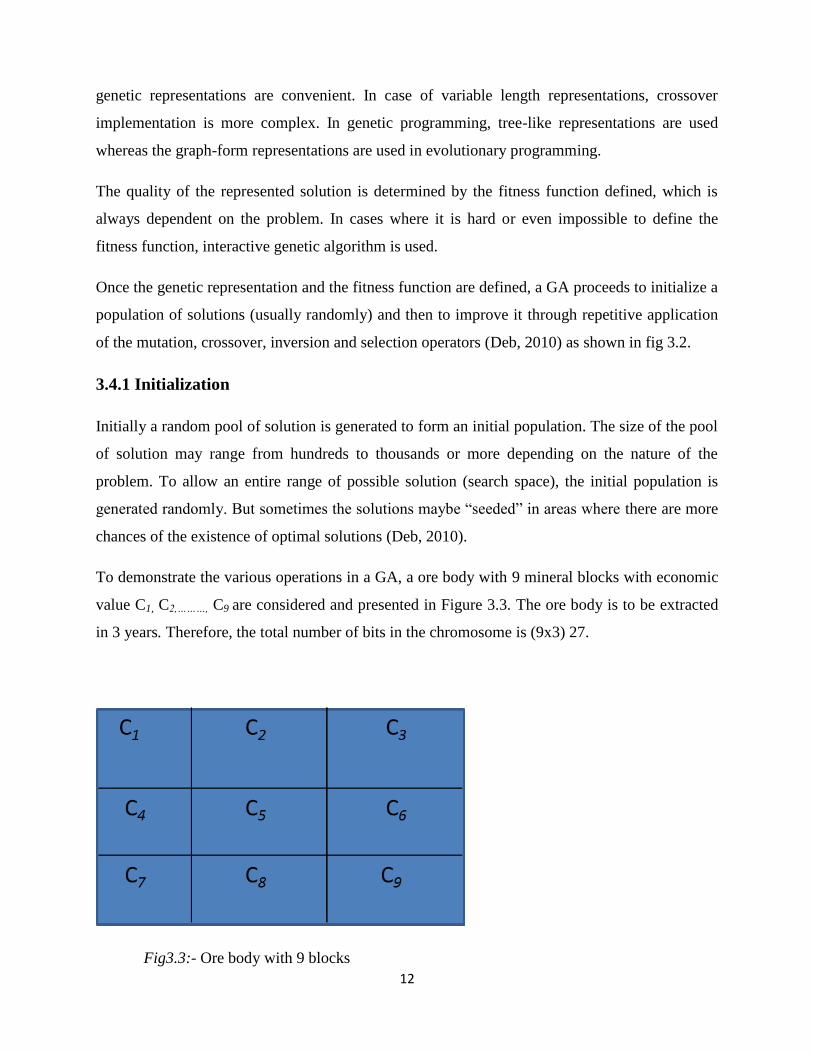
To demonstrate the various operations in a GA, a ore body with 9 mineral blocks with economic

value C1, C2,………, C9 are considered and presented in Figure 3.3. The ore body is to be extracted

in 3 years. Therefore, the total number of bits in the chromosome is (9x3) 27.

Fig3.3:- Ore body with 9 blocks

13

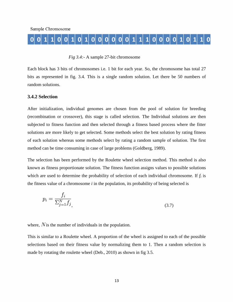
Fig 3.4:- A sample 27-bit chromosome

Each block has 3 bits of chromosomes i.e. 1 bit for each year. So, the chromosome has total 27

bits as represented in fig. 3.4. This is a single random solution. Let there be 50 numbers of

random solutions.

3.4.2 Selection

After initialization, individual genomes are chosen from the pool of solution for breeding

(recombination or crossover), this stage is called selection. The Individual solutions are then

subjected to fitness function and then selected through a fitness based process where the fitter

solutions are more likely to get selected. Some methods select the best solution by rating fitness

of each solution whereas some methods select by rating a random sample of solution. The first

method can be time consuming in case of large problems (Goldberg, 1989).

The selection has been performed by the Roulette wheel selection method. This method is also

known as fitness proportionate solution. The fitness function assigns values to possible solutions

which are used to determine the probability of selection of each individual chromosome. If fi is

the fitness value of a chromosome i in the population, its probability of being selected is

, (3.7)

where, is the number of individuals in the population.

This is similar to a Roulette wheel. A proportion of the wheel is assigned to each of the possible

selections based on their fitness value by normalizing them to 1. Then a random selection is

made by rotating the roulette wheel (Deb., 2010) as shown in fig 3.5.

14

Fig3.5:- Roulette wheel selection

Fig Reference:- http://www.edc.ncl.ac.uk/assets/hilite_graphics/rhjan07g02.png

Fig 3.6:- Two sample chromosome having highest probability of selection

For an example, say chromosome 26 and 35 (fig 3.6) have the highest share in the roulette wheel

and so they have the maximum probability to get selected for reproduction

3.4.3 Reproduction

Once selection is done, the selected solutions are used to generate second generation of

population of solutions which is called reproduction. This is achieved through genetic operators:

crossover (also called recombination), and/or mutation.

15

These processes result in producing next generation of population of solutions that is different

from the initial generation. Generally the average fitness increases by this procedure for the

population, since in reproduction only the selected fitter solutions are considered (Goldberg,

1989).

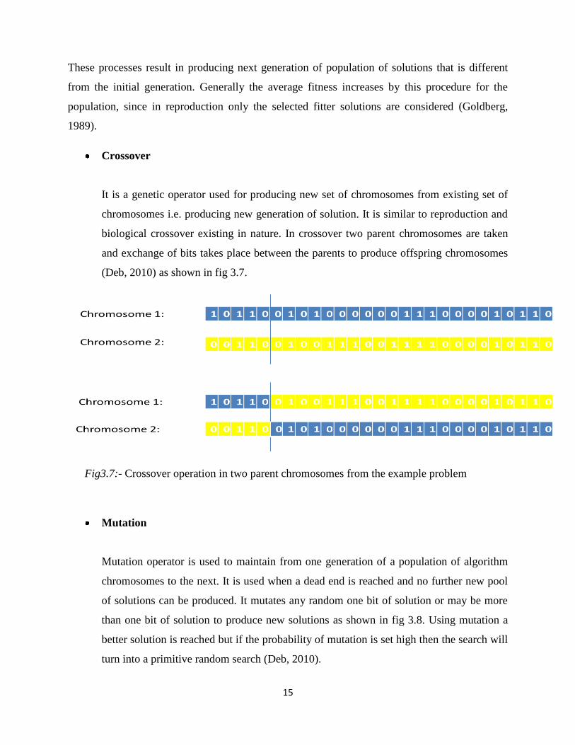
Crossover

It is a genetic operator used for producing new set of chromosomes from existing set of

chromosomes i.e. producing new generation of solution. It is similar to reproduction and

biological crossover existing in nature. In crossover two parent chromosomes are taken

and exchange of bits takes place between the parents to produce offspring chromosomes

(Deb, 2010) as shown in fig 3.7.

Fig3.7:- Crossover operation in two parent chromosomes from the example problem

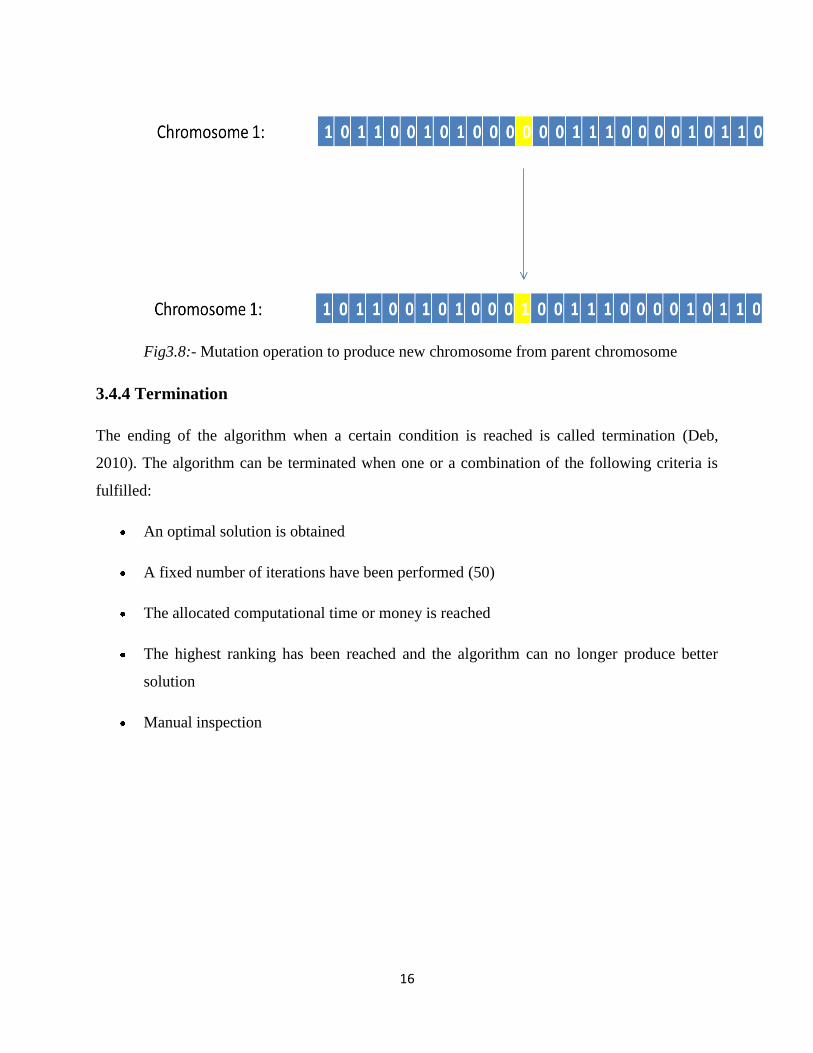
Mutation

Mutation operator is used to maintain from one generation of a population of algorithm

chromosomes to the next. It is used when a dead end is reached and no further new pool

of solutions can be produced. It mutates any random one bit of solution or may be more

than one bit of solution to produce new solutions as shown in fig 3.8. Using mutation a

better solution is reached but if the probability of mutation is set high then the search will

turn into a primitive random search (Deb, 2010).

16

Fig3.8:- Mutation operation to produce new chromosome from parent chromosome

3.4.4 Termination

The ending of the algorithm when a certain condition is reached is called termination (Deb,

2010). The algorithm can be terminated when one or a combination of the following criteria is

fulfilled:

An optimal solution is obtained

A fixed number of iterations have been performed (50)

The allocated computational time or money is reached

The highest ranking has been reached and the algorithm can no longer produce better

solution

Manual inspection

17

Fig3.9:- Flowchart for working principles of GA

The flowchart in fig 3.9 depicts the whole working principles of GA and steps involved are

outlined here:-

1. First of all the population of solution is initialized.

2. The generation counter is set to 0

3. The population is evaluated.

4. It is checked under the fitness function. If the condition is satisfied, the algorithm

terminates.

5. If the condition is not fulfilled, the population goes through reproduction, crossover and

mutation processes.

6. The generation counter is incremented by 1 and step 3 to 5 is repeated.

18

CHAPTER 4

CASE STUDY

19

4. CASE STUDY

The study was carried out on an iron ore mine situated in the south-eastern part of India. The

deposit lies between latitude 18041

’ and 18

042

’, and longitude 81

042

’ and 81

012

’30

”. This is a

hilly deposit with highly undulating ground level. The highest point of the deposit is 1269 m

above the mean sea level (MSL) and the lowest point, upto which mineralization found during

the investigation, is at 950 m reduced level. Most of the area of the deposit is covered by green

vegetation. The area is drained by seasonal nalahs which are flowing both the sides of the

deposit. The geological study of the deposit revealed that this iron ore deposit was formed

during the precambrian age. This series of ore consists of iron ore, unenriched banded iron

formation rocks (Banded Hematite quartzite), shale, tuff and quartzite. The major iron ore

bodies occur along the top of the range and generally at the bottom of the underlying shale. The

deposit is situated in the southern ridge of the range. There are numbers of folds, faults present

in the mine which indicates that the deposit is highly disturbed in nature. There were 77

borehole data available from the mine for conducting this study. The boreholes are located in a

grid pattern; however, the spacing of the boreholes varies from 200-250 meters. The average

length of the boreholes is about 100 meters. Samples from the boreholes were collected in cores

of less than 1-meter. The mine has seven different lithologies namely Steel Gray Hematite

(SGH) Blue hematite (BH), Laminated Hematite (LH), Laterite (L), Blue Dust (BD), Shale

(SHL) and Banded Hematite Quartzite (BHQ). Most of the high grade iron ore is associated

with still gray, blue and laminated hematite. The average depth of the mine is 160 m. The mine

has fourteen working benches with bench height of 12 meter.

20

CHAPETR 5

RESULTS

ULTIMATE PIT MODEL

NET PRESENT VALUE

STRIPPING RATIO

MINING CONSTRAINT

21

5. RESULTS

The resource of the deposit was estimated using ordinary kriging method using the 5 m

composited borehole data (Chatterjee, 2006). The number of estimated blocks in the deposit is

47275. The size of the estimated block is 50 m x 50 m x 10 m. The production scheduling was

performed for 4 years and hence the sample chromosomes had 189100 (47275x4) bits. Now the

mining constraints and slope constraints were determined. The mine had a maximum capacity of

producing 6.25x108 tons of material per year. To prevent the machines from being idle, the mine

should produce 6.20x108 tons of material per year. The maximum number of iterations was set to

50. The mutation rate for the problem was defined to be 0.1. The amount of time taken to solve

this problem is 31 minute.

The fig. 5.1 shows that the mine produced the tonnage of material almost at a constant rate. The

value of the mineral produced throughout the life of the mine is always within the range of

mining constraints. From the figure, it is observed that the mine has produced 6.23x108 tons of

material every year i.e. the mining constraint was followed.

Fig5.1:-Tonnage extracted per year grapgh

22

The ultimate pit of a mine is defined to be that contour which is the result of extracting the

volume of material which provides the total maximum profit whilst satisfying the operational

requirement of safe wall slopes. The ultimate pit limit gives the shape of the mine at the end of

its life.

Color Index:

No. of year: 1 2 3 4

Fig5.2:- 3D view of the ultimate pit

Color Index:

No. of year: 1 2 3 4

Fig5.3:- Ultimate Pit in Y-Z axis

The ultimate pit model obtained as shown in fig. 5.2 and 5.3 show the section of the mine that

are going to be extracted over the period of 4 years. The deep blue color represents the section of

the mine that is scheduled to be extracted in the 1st year. The lighter blue color indicates the ore

body scheduled to be extracted in the 2nd

year. The yellow and brown colored sections shows the

ore scheduled to be extracted in the 3rd

and 4th

year. From the ultimate pit model, it was observed

23

that the slope constraint has been followed and also no ore block has been extracted twice and

hence the reserve constraint has been followed

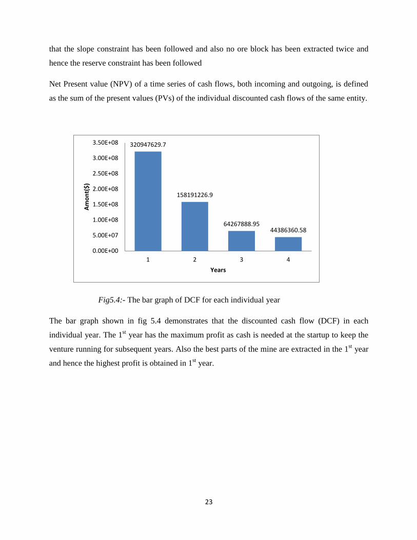
Net Present value (NPV) of a time series of cash flows, both incoming and outgoing, is defined

as the sum of the present values (PVs) of the individual discounted cash flows of the same entity.

Fig5.4:- The bar graph of DCF for each individual year

The bar graph shown in fig 5.4 demonstrates that the discounted cash flow (DCF) in each

individual year. The 1st year has the maximum profit as cash is needed at the startup to keep the

venture running for subsequent years. Also the best parts of the mine are extracted in the 1st year

and hence the highest profit is obtained in 1st year.

320947629.7

158191226.9

64267888.95 44386360.58

0.00E+00

5.00E+07

1.00E+08

1.50E+08

2.00E+08

2.50E+08

3.00E+08

3.50E+08

1 2 3 4

Am

on

t($

)

Years

24

Fig5.5:- The cumulative line graph of NPV for the mine

The cumulative graph in fig 5.5 shows that the NPV of the mine never goes down i.e. it always

remain in profit The Net Present Value of the mine for 4 years was calculated to be 551 million

$.

Stripping ratio refers to the ratio of the volume of overburden (or waste material) required to be

handled in order to extract some volume of ore.

Fig5.6:- The Stripping Ratio for each Year.

320947629.7

464757836 517871793.8

551219923.5

0.00E+00

1.00E+08

2.00E+08

3.00E+08

4.00E+08

5.00E+08

6.00E+08

1 2 3 4

Am

ou

nt(

$)

Year

Net Present Value

Series1

0.52

1.52

2.81

3.88

0

0.5

1

1.5

2

2.5

3

3.5

4

4.5

1 2 3 4

Stri

pp

ing

Rat

io

Years

Stripping Ratio

25

The Stripping Ratio in the first year was 0.52 which rises up to 3.88 by the 4th

year as shown in

fig 5.6. This is because as the time passes, the ore blocks get extracted leaving the waste blocks.

Hence for further removal of ore blocks, more overburden removal is required in subsequent

years. The average Stripping Ratio over the period of 4 years was found to be 1.72.

26

CHAPTER 6

CONCLUSION

27

6. CONCLUSION

A study was carried out to solve an optimization problem of production scheduling of an open pit

mine using a meta heuristic approach. The meta heuristic approach selected was Genetic

Algorithm. Genetic Algorithms are known to provide solutions to complex problems handling

large variables and constraints in significantly less time.

The iron ore mine had 47275 numbers of blocks that needed to be extracted over a period of 4

years i.e. the total number of variables in the search space is 189100. This problem could not

have been solved by tradition methods. The computational time required for solving the

production scheduling problem of Iron Ore Mine having 47275 blocks for a period of four years

after 50 iterations was just 31 minutes for a Pentium i3 2.1 GHz processor which emphasizes that

the computational time for solving the problem using GA is significantly less. The results

obtained were used to calculate the ultimate pit, net present value and Stripping ratio. No

constraint was violated in the algorithm.

Hence incorporating the constraint equations in the objective to and solving the derived

unconstrained expression using genetic algorithm can be a viable method of optimization

problems of an open pit mine.

The limitation of the present work is that the obtained results have not been compared with any

optimum solution. To know the ability of the proposed approach, a valid comparison study is

required.

28

CHAPTER 7

REFERENCES

29

7. REFERENCES

I. Chatterjee, S., Geostatistical and image based quality control models for Indian mineral

industry. Unpublished Ph.D. Thesis dissertation, IIT Kharagour, India, 2006, 272 pp.

II. Deb, K., Multi-Objective Optimization using Evolutionary Algorithms, Wiley India,

Evolutionary Algorithm (2010) pp.84-126

III. Goldberg, D.E., Genetic Algorithms in Search, Optimization and Machine Learning.

Kluwer Academic Publishers (1989).

IV. De Jong, K., Learning with genetic algorithms: An overview, Machine Learning (1988)

pp.121–138.

V. Whittle, J., A Decade of Open Pit Mine Planning and Optimization -The Craft of Turning

Algorithms into packages, 28Th

APCOM Proceedings - Colorado School of Mines,

Golden, CO (1999), pp 15-23

VI. Ali A., Emary I., and El-Kareem M., Application of Genetic Algorithm in Solving Linear

Equation Systems, MASAUM Journal of Basic and Applied Science, 1 (2009), pp. 179-

185

VII. Glover, F., and Kochenberger, G.A., Handbook of metaheuristics. Springer, International

Series in Operations Research & Management Science (2003). ISBN 978-1-4020-7263-5.

VIII. Pana, M., T., The simulation approach to open pit design, in: Proceedings of 5th

International Symposium on Computer Applications in the Mineral Industry, Tuscon, AZ

(1965) pp. ZZ1–ZZ24.

IX. Barbaro,R.,W. and Ramani, R.,V., Generalized multi-period MIP model for production

scheduling and processing facilities selection and location, Mining Engineering 38(2)

(1986) ,pp.107–114.

X. Mukherjee, K., Application of an interactive method for MOILP in project selection

decision – A case from Indian coal mining industry, International Journal of Production

Economics 36 (1994), pp.203–211.

XI. Pendharkar, P., C., A fuzzy linear programming application for production scheduling in

coal mines, Computers & Operations Research 24(2) (1997), pp.1141–1149.

XII. Lamghari, L. and Dimitrakopoulos, R. , Metaheuristic for the Open Pit Mine Production

Scheduling Problem with Uncertain Supply, McGill, COSMO, Research Report No. 4

Vol 1 (2010), pp 110-149

30

XIII. Seymour, F., Pit Limit Parameterization From Modified 3d Lerchs-Grossmann

Algorithm, SME Manuscript (1995), pp. 1-11

XIV. Ramazan, S. and Dimitrakopoulos, R., Stochastic optimization of long term production

scheduling for open pit mines with a new integer programming formulation. Orebody

Modelling and Strategic Mine Planning, The Australasian Institute of Mining and

Metallurgy, Spectrum Series, 14, 2nd Edition (2007), pp. 385-391.

XV. Boland, N., Dumitrescu, I. , Froyland, G. , Gleixner, A.M., LP-based disaggregation

approaches to solving the open pit mining production scheduling problem with block

processing selectivity , Computers and operations research 36 (4) (2007), pp. 1064-1089.

XVI. Albor, F. and Dimitrakopoulos R. Stochastic mine design optimization based on

simulated annealing: Pit limits, production schedules, multiple orebody scenarios and

sensitivity analysis. IMM Transactions, Mining Technology, 118 (2) (2009), pp. 80-91.

XVII. Pendharkar, P.C. and Rodger, J. A., Nonlinear programming and genetic search

application for production scheduling in coal mine, Annals of Operations Research 95

(2000) pp. 251-267.

XVIII. Hiller F.S. and Lieberman, G.J. Introduction to Operations Research (McGraw-Hill,

1995).

XIX. Reeves, C.R., Genetic Algorithms for the Operations Researcher, INFORMS Journal on

Computing 9(3) (1997), pp 231-250 ,