oovveerrvviieeww ooff tthhee - usgs 17, alessandra corsi 7, james costner 20, dale cox 17, tapash...

OOvveerrvviieeww ooff tthhee

AARRkkSSttoorrmm SScceennaarriioo

Open File Report 2010-1312

U.S. Department of the Interior U.S. Geological Survey

This page intentionally left blank

Overview of the Arkstorm Scenario Prepared for the U.S. Geological Survey Multihazards Demonstration Project Lucile Jones, Chief Scientist Dale Cox, Project Manager

By

Keith Porter18, Anne Wein17, Charles Alpers17, Allan Baez1, Patrick Barnard17, James Carter17, Alessandra Corsi7, James Costner20, Dale Cox17, Tapash Das14, Michael Dettinger17, James Done12, Charles Eadie8, Marcia Eymann5, Justin Ferris17, Prasad Gunturi20, Mimi Hughes13, Robert Jarrett17, Laurie Johnson10, Hanh Dam Le-Griffin16, David Mitchell11, Suzette Morman17, Paul Neiman13, Anna Olsen18, Suzanne Perry17, Geoffrey Plumlee17, Martin Ralph13, David Reynolds13, Adam Rose19, Kathleen Schaefer6, Julie Serakos20, William Siembieda4, Jonathan Stock17, David Strong17, Ian Sue Wing2, Alex Tang9, Pete Thomas20, Ken Topping15, and Chris Wills3.

1 B.A. Risk Management 11 M-Cubed 2 Boston University 12 National Center for Atmospheric

Research 3 California Geological Survey 13 National Oceanic and Atmospheric

Administration 4 California Polytechnic State University 14 Scripps Institute of Oceanography 5 Center for Sacramento History 15 Topping Associates International 6 Federal Emergency Management Agency 16 TTW, Inc. 7 Instituto de Pesquisas Tecnologicas, Brazil 17 U.S. Geological Survey 8 Hamilton Swift Land Use and Development 18 University of Colorado at Boulder 9 L&T Consulting 19 University of Southern California 10 Laurie Johnson Consulting 20

Willis Group

ii

U.S. Department of the Interior KEN SALAZAR, Secretary

U.S. Geological Survey Marcia K. McNutt, Director

U.S. Geological Survey, Reston, Virginia 2011

For product and ordering information: World Wide Web: http://www.usgs.gov/pubprod Telephone: 1-888-ASK-USGS

For more information on the USGS—the Federal source for science about the Earth, its natural and living resources, natural hazards, and the environment: World Wide Web: http://www.usgs.gov Telephone: 1-888-ASK-USGS

Suggested citation: Porter, Keith, Wein, Anne, Alpers, Charles, Baez, Allan, Barnard, Patrick, Carter, James, Corsi, Alessandra, Costner, James, Cox, Dale, Das, Tapash, Dettinger, Michael, Done, James, Eadie, Charles, Eymann, Marcia, Ferris, Justin, Gunturi, Prasad, Hughes, Mimi, Jarrett, Robert, Johnson, Laurie, Dam Le-Griffin, Hanh, Mitchell, David, Morman, Suzette, Neiman, Paul, Olsen, Anna, Perry, Suzanne, Plumlee, Geoffrey, Ralph, Martin, Reynolds, David, Rose, Adam, Schaefer, Kathleen, Serakos, Julie, Siembieda, William, Stock, Jonathan, Strong, David, Sue Wing, Ian, Tang, Alex, Thomas, Pete, Topping, Ken, and Wills, Chris; Jones, Lucile, Chief Scientist, Cox, Dale, Project Manager, 2011, Overview of the ARkStorm scenario: U.S. Geological Survey Open-File Report 2010-1312, 183 p. and appendixes [http://pubs.usgs.gov/of/2010/1312/].

Any use of trade, product, or firm names is for descriptive purposes only and does not imply endorsement by the U.S. Government.

Although this report is in the public domain, permission must be secured from the individual copyright owners to reproduce any copyrighted material contained within this report.

http://www.usgs.gov/pubprod�

http://www.usgs.gov/�

http://pubs.usgs.gov/of/2010/1312/�

iii

Acknowledgments

This document reflects the contributions of a large interdisciplinary team of lifeline experts and agencies, including:

California Department of Public Health: Clifford Bowen and Joseph Crisologo

California Department of Transportation: Roy Bibbens, Mandy Chu, John Duffy, Jim Morris, Gustavo Ortega, Cliff Roblee, Earl Sherman, Loren Turner, and Bill Varley

California Department of Water Resources: Bill Croyle, Sonny Fong, Andy Mangney, Michael Mierzwa, Ricardo Pineda, and Tawnly Pranger

California Emergency Management Agency: Robert Mead

California Environmental Legacy Project: Kit Tyler

California Environmental Protection Agency: Duncan Austin and Antonia Vorster

California Extreme Precipitation Symposium: Gary Estes

California Geological Survey: Dave Branum and Ante Perez

California Institute of Technology: Margaret Vinci

California Polytechnic State University: Bud Evans, Robb Moss

California State University at Sacramento Police: Kelly Clark

California Utilities Emergency Association: Don Boland

Coachella Valley Water District: Mike Herrera

Contra Costa County Health: Eric Jonsson

Contra Costa County Sheriff: Marcelle Indelicato and Rick Kovar

East Valley Water: Gary Sturdivan Golden State Water: John Spitter

Institute for the Future: Jason Tester

Los Angeles City Building and Public Works: Tom Cotter

Los Angeles City Bureau of Sanitation: Chuck Turhollow

Los Angeles City Department of Water and Power: Craig Davis, Melinda Rho, Minas Sirakie, and Julie Spacht

Los Angeles County Department of Public Works: Ben Willardson

Los Angeles Department of Water and Power: Kevin Garrity

Metropolitan Water District of Southern California: Christopher Hill and George del Toro

Michael Baker Corporation: Travis Clark and Jagdeep Sidhu

National Oceanic and Atmospheric Administration: Rob Hartman and Alan Hayes

iv

Sacramento County Environmental Management Department: Val Sielal

Sacramento County Water Resources: George Booth

Sacramento Municipal Utility District: Selby Mohr

San Bernardino County Department of Public Works: Erwin Fogerson

San Diego County Water Authority: Lorrie Teates

San Francisco Department of Public Works: Greg Braswell

San Francisco Public Utilities Commission: Bruce McGurk

San Joaquin County Environmental Health Department: Linda Turkatte

San Jose Water Company: Jim Wollbrinck

Santa Clara Valley Water District: Michael Hamer

Southern California Edison: John A. Bocka, Tom Botello, Don Conner, and Roger Lee

University of California at Davis: Robert Lim

URS Corporation: Paul Jacks

U.S. Army Corps of Engineers: Sean Mann

U.S. Environmental Protection Agency: Harry Allen, Pete Guria, Bruce Macler, Rich Martyn, and Dan Meer

U.S. Geological Survey: Gerald Bawden, Sue Cannon, Rick Champion, Laura Dinitz, Dawn MacCarthy, and Tanja Wolfmeyer

Water Forum: Mark Roberson

v

Abstract

The U.S. Geological Survey, Multi Hazards Demonstration Project (MHDP) uses hazards science to improve resiliency of communities to natural disasters including earthquakes, tsunamis, wildfires, landslides, floods and coastal erosion. The project engages emergency planners, businesses, universities, government agencies, and others in preparing for major natural disasters. The project also helps to set research goals and provides decision-making information for loss reduction and improved resiliency. The first public product of the MHDP was the ShakeOut Earthquake Scenario published in May 2008. This detailed depiction of a hypothetical magnitude 7.8 earthquake on the San Andreas Fault in southern California served as the centerpiece of the largest earthquake drill in United States history, involving over 5,000 emergency responders and the participation of over 5.5 million citizens.

This document summarizes the next major public project for MHDP, a winter storm scenario called ARkStorm (for Atmospheric River 1,000). Experts have designed a large, scientifically realistic meteorological event followed by an examination of the secondary hazards (for example, landslides and flooding), physical damages to the built environment, and social and economic consequences. The hypothetical storm depicted here would strike the U.S. West Coast and be similar to the intense California winter storms of 1861 and 1862 that left the central valley of California impassible. The storm is estimated to produce precipitation that in many places exceeds levels only experienced on average once every 500 to 1,000 years.

Extensive flooding results. In many cases flooding overwhelms the state’s flood-protection system, which is typically designed to resist 100- to 200-year runoffs. The Central Valley experiences hypothetical flooding 300 miles long and 20 or more miles wide. Serious flooding also occurs in Orange County, Los Angeles County, San Diego, the San Francisco Bay area,

and other coastal communities. Windspeeds in some places reach 125 miles per hour, hurricane-force winds. Across wider areas of the state, winds reach 60 miles per hour. Hundreds of landslides damage roads, highways, and homes. Property damage exceeds $300 billion, most from flooding. Demand surge (an increase in labor rates and other repair costs after major natural disasters) could increase property losses by 20 percent. Agricultural losses and other costs to repair lifelines, dewater (drain) flooded islands, and repair damage from landslides, brings the total direct property loss to nearly $400 billion, of which $20 to $30 billion would be recoverable through public and commercial insurance. Power, water, sewer, and other lifelines experience damage that takes weeks or months to restore. Flooding evacuation could involve 1.5 million residents in the inland region and delta counties. Business interruption costs reach $325 billion in addition to the $400 billion property repair costs, meaning that an ARkStorm could cost on the order of $725 billion, which is nearly 3 times the loss deemed to be realistic by the ShakeOut authors for a severe southern California earthquake, an event with roughly the same annual occurrence probability.

K Street, Sacramento, looking east

1861-1862

vi

The ARkStorm has several public policy implications: (1) An ARkStorm raises serious questions about the ability of existing federal, state, and local disaster planning to handle a disaster of this magnitude. (2) A core policy issue raised is whether to pay now to mitigate, or pay a lot more later for recovery. (3) Innovative financing solutions are likely to be needed to avoid fiscal crisis and adequately fund response and recovery costs from a similar, real, disaster. (4) Responders and government managers at all levels could be encouraged to conduct risk assessments, and devise the full spectrum of exercises, to exercise ability of their plans to address a similar event. (5) ARkStorm can be a reference point for application of Federal Emergency Management Agency (FEMA) and California Emergency Management Agency guidance connecting federal, state and local natural hazards mapping and mitigation planning under the National Flood Insurance Plan and Disaster Mitigation Act of 2000. (6) Common messages to educate the public about the risk of such an extreme disaster as the ARkStorm scenario could be developed and consistently communicated to facilitate policy formulation and transformation.

These impacts were estimated by a team of 117 scientists, engineers, public-policy experts, insurance experts, and employees of the affected lifelines. In many aspects the ARkStorm produced new science, such as the model of coastal inundation. The products of the ARkStorm are intended for use by emergency planners, utility operators, policymakers, and others to inform preparedness plans and to enhance resiliency.

vii

Table of Contents

Acknowledgments ........................................................................................................................................... iii Abstract ............................................................................................................................................................... v Index of Figures ................................................................................................................................................. x Index of Tables ................................................................................................................................................ xv Introduction ........................................................................................................................................................ 1 ARkStorm Meteorology .................................................................................................................................... 3

FLOODING ....................................................................................................................................................... 7 WINDSPEED ................................................................................................................................................. 11

Coastal Inundation .......................................................................................................................................... 12 RESEARCH NEEDS RELATED TO COASTAL INUNDATION .................................................................. 16

Landsliding ........................................................................................................................................................ 16 RESEARCH NEEDS RELATED TO LANDSLIDING ................................................................................... 22

Three Approaches to Estimating Damage .................................................................................................. 23 Lifeline Panel Process .................................................................................................................................... 23 Highway Damage ............................................................................................................................................ 24

HIGHWAY FACILITIES AND SOURCES OF DAMAGE ............................................................................ 24 HIGHWAY DAMAGE AND RESTORATION SCENARIO ......................................................................... 24 LIFELINE INTERACTION INVOLVING HIGHWAYS ................................................................................. 33 LIMITATIONS OF HIGHWAY RESTORATION TIMELINE ...................................................................... 34 OPPORTUNITIES TO ENHANCE HIGHWAY RESILIENCY ..................................................................... 34

Power ................................................................................................................................................................ 35 POWER FACILITIES AND SOURCES OF DAMAGE ................................................................................. 35 POWER DAMAGE AND RESTORATION SCENARIO .............................................................................. 38 LIFELINE INTERACTION INVOLVING POWER ........................................................................................ 41 OPPORTUNITIES TO ENHANCE POWER RESILIENCY .......................................................................... 41 LIMITATIONS OF ESTIMATES WITH RESPECT TO POWER ................................................................ 42

Wastewater Treatment .................................................................................................................................. 42 WASTEWATER FACILITIES AND SOURCES OF DAMAGE ................................................................... 42 WASTEWATER DAMAGE AND RESTORATION SCENARIO ................................................................ 44 LIFELINE INTERACTION INVOLVING WASTEWATER TREATMENT .................................................. 47 RESILIENCY AND RESEARCH NEEDS FOR WASTEWATER SERVICE ................................................ 47

Water Supply.................................................................................................................................................... 48 WATER FACILITIES AND SOURCES OF DAMAGE ................................................................................. 48 WATER SUPPLY DAMAGE AND RESTORATION SCENARIO .............................................................. 48 LIFELINE INTERACTION INVOLVING WATER SUPPLY ........................................................................ 56 ENHANCING RESILIENCY FOR WATER SUPPLY ................................................................................... 56 RESEARCH NEEDS FOR WATER SUPPLY ............................................................................................... 57

Dams .................................................................................................................................................................. 57 DAM DAMAGE SCENARIO ........................................................................................................................ 58 LIFELINE INTERACTION RELATED TO DAM DAMAGE ......................................................................... 59

viii

Levees ............................................................................................................................................................... 59 THE DELTA LEVEE DAMAGE AND REPAIR SCENARIO ........................................................................ 59

Flooded Islands ........................................................................................................................................ 62 Repair Costs and Timing ......................................................................................................................... 62

MITIGATION OF LEVEE FAILURE .............................................................................................................. 64 Telecommunications ...................................................................................................................................... 64

TELECOMMUNICATIONS ASSETS EXPOSED TO LOSS ....................................................................... 65 MECHANISMS FOR TELECOMMUNICATIONS SERVICE INTERRUPTION ....................................... 66 TELECOMMUNICATIONS SERVICE RESTORATION SCENARIO ......................................................... 67 LIFELINE INTERACTION INVOLVING TELECOMMUNICATIONS ........................................................ 70 OPPORTUNITIES TO ENHANCE TELECOMMUNICATIONS RESILIENCY .......................................... 70

Agricultural Damages and Losses ............................................................................................................... 70 HISTORIC AGRICULTURAL DAMAGES FROM CALIFORNIA FLOODS ................................................ 71 METHODOLOGY ........................................................................................................................................... 73

Location, Extent, Depth, and Duration of Flooded Agricultural Land ............................................. 74 Field Cleanup and Repair Costs ............................................................................................................ 75 Damages to Annual Crops ..................................................................................................................... 75 Damages to Perennial Crops ................................................................................................................. 76 Damages to Livestock ............................................................................................................................. 77

ARkSTORM AGRICULTURAL DAMAGE ESTIMATES ............................................................................ 78 Damaged Land ......................................................................................................................................... 78 Statewide Agricultural Damages.......................................................................................................... 78 County Agricultural Damages ............................................................................................................... 81 Effects of Delays in Delta Island Dewatering ..................................................................................... 86 SUMMARY ................................................................................................................................................ 87

MITIGATING AGRICULTURAL DAMAGES .............................................................................................. 87 RESEARCH NEEDS RELATED TO AGRICULTURAL DAMAGES ............................................................ 88

Building and Content Repair Costs .............................................................................................................. 89 PROPERTY-DAMAGE METHODOLOGY .................................................................................................... 89 PROPERTY-DAMAGE SCENARIO ............................................................................................................. 91 RESILIENCY AND RESEARCH NEEDS FOR BUILDING DAMAGE........................................................ 95 DEMAND SURGE ......................................................................................................................................... 97 COMPARISON WITH PAST EVENTS........................................................................................................ 98

Insurance Impacts .......................................................................................................................................... 98 INTRODUCTION ........................................................................................................................................... 98 CALIFORNIA FLOOD AND WIND INSURANCE COVERAGE ................................................................. 99 INSURANCE LOSS FROM THE ARKSTORM SCENARIO ..................................................................... 100 HISTORICAL PRECEDENT AND ECONOMIC RESILIENCY .................................................................. 102 RESEARCH NEEDS RELATED TO INSURANCE ..................................................................................... 102

Evacuation ...................................................................................................................................................... 103 POPULATION LIVING IN FLOODED AREAS .......................................................................................... 103 SOCIAL INDICATORS ................................................................................................................................ 105

ix

SHELTER REQUIREMENTS ...................................................................................................................... 111 RESEARCH NEEDS RELATED TO EVACUATION .................................................................................. 113

Business Interruption Costs ........................................................................................................................ 114 INTRODUCTION ......................................................................................................................................... 114 HAZARD LOSS ESTIMATION .................................................................................................................. 114

BASIC CONSIDERATIONS ................................................................................................................... 114 CONDUITS OF ECONOMIC SHOCKS .................................................................................................. 116

THE DYNAMIC COMPUTABLE GENERAL EQUILIBRIUM MODEL .................................................... 117 METHODOLOGICAL DETAILS FOR INDIVIDUAL LOSS CATEGORIES .............................................. 118 RESILIENCE ................................................................................................................................................ 120 ADJUSTMENT FOR MULTIPLE SOURCES OF BUSINESS INTERRUPTION .................................... 121 MACROECONOMIC IMPACTS ................................................................................................................ 124 SUMMARY OF RESULTS .......................................................................................................................... 137 CONCLUSION ............................................................................................................................................. 138

Truck Traffic Economic Impacts from Reduced Highway Capacities ................................................. 139 Method of Analysis ................................................................................................................................... 139 Truck travel time, distance, cost, and economic impacts ................................................................. 141 RESEARCH NEEDS RELATED TO TRAFFIC ECONOMIC IMPACTS ................................................... 146

Environmental and Health Issues ............................................................................................................... 148 PLAUSIBLE ENVIRONMENTAL-HEALTH ISSUES AND IMPACTS ................................................... 148 APPROACH FOR ENVIRONMENTAL AND HEALTH IMPACTS .......................................................... 149

Public Policy Issues ...................................................................................................................................... 151 OVER-ARCHING POLICY CONSIDERATION .......................................................................................... 151 PRIORITY POLICY ISSUES: MITIGATION .............................................................................................. 157 PRIORITY POLICY ISSUES: PREPAREDNESS AND RESPONSE ........................................................ 160 PRIORITY POLICY ISSUES: RECOVERY .................................................................................................. 162 PRIORITY POLICY ISSUES: RISK AWARENESS ................................................................................... 166 POSSIBLE COURSES OF ACTION ........................................................................................................... 169

Summary ......................................................................................................................................................... 171 KEY FINDINGS ............................................................................................................................................ 171 CONCLUSION ............................................................................................................................................. 172

References Cited ........................................................................................................................................... 173

x

Index of Figures

Figure 1. K Street, Sacramento, looking east, in January or February 1862. (Photographers Lawrence and Houseworth, The Bancroft Library Pictorial Collection, University of California, Berkeley) ............................................................................................................................................................. 3

Figure 2. This map of the Pacific region shows an Atmospheric River originating over the central Pacific on February 16, 2004, indicated by high (green) vertically-integrated water-vapor contents, in grams per square centimeter of water vapor, in the atmosphere extending from around Hawaii to the central California coast near the town of Cazadero (CZD). ........................................................... 4

Figure 3. Weather Research and Forecasting (WRF) model domains used in simulations of ARkStorm meteorology, with nested model domains indicated by boxes and the topography resolved by the grids in each domain indicated by contours. Grid spacings are 2 km in smaller black box, 6 km in larger black box, 18 km in blue area, and 54 km in red area. ................................... 5

Figure 4. ARkStorm stitched-storm calendar, with moderately wet conditions of autumn and early winter “preconditioning” the watersheds of California for rapid flood generation indicated by blue shading, followed by the two intense-storm periods that were combined to make up the ARkStorm scenario indicated in red shading. These calendars represent actual storms of 1969 and 1986, which provided the basis for the ARkStorm modeling. .............................................................................. 6

Figure 5. For locations around Califonria, colors depict recurrence intervals in years of maximum 3-day runoff during the ARkStorm scenario. ................................................................................................ 7

Figure 6. This snapshot of available flood models shows that various models cover the Central Valley (gridded area) but not the rest of the state (California Department of Water Resources, 2010a). .................................................................................................................................................................. 9

Figure 7. Hydrologic Unit Code 6 watershed boundaries, with ARkStorm flooding parameter values, depth of flooding and length of time flooded. ............................................................................... 10

Figure 8. Blue areas indicate ARkStorm flooding as projected by models used in the scenario. ... 11

Figure 9. ARkStorm peak 10-meter elevation, 3-second gust wind speeds. ........................................ 12

Figure 10. Extent of the CoSMoS model applied to the ARkStorm scenario. See Barnard and others (2009) for details and additional maps. ........................................................................................... 13

Figure 11. CoSMoS-estimated coastal inundation at the Ports of Los Angeles and Long Beach. .. 14

Figure 12. CoSMoS-estimated coastal inundation at Seal Beach. ........................................................ 14

Figure 13. CoSMoS-estimated coastal inundation at Mission Bay, San Diego. .................................. 15

xi

Figure 14. CoSMoS-estimated coastal inundation at Coronado and Imperial Beaches. .................. 15

Figure 15. Categories of landslide treated by ARkStorm (Wills and others, 2001 modified after Varnes, 1958 and Colorado Geological Survey, 1988) ............................................................................... 18

Figure 16. Deep-seated landslide in Ventura Calif., January 2005 (left, photo credit: J. Stock, USGS), and 1982 debris flow in Pacifica, Calif., that killed 3 (right, photo courtesy of Woodward Clyde Consultants). ......................................................................................................................................... 19

Figure 17. Deep-seated Landslide Susceptibility Map of California. Black lines denote county boundaries. Higher numbers and hotter colors indicate greater susceptibility to deep-seated landslides. ......................................................................................................................................................... 20

Figure 18. Quaternary, Pliocene, and Miocene sedimentary rocks (hachured area) superimposed on the forecast for landslide abundance resulting from the ARkStorm. Cells in the hachured area have rock types similar to the calibration area at Santa Paula. Cells outside these zones likely overestimate the number of landslides because (1) rock units produce stronger soils and( 2) different processes (for example, rock fall) dominate erosion. Gray areas have no unstable cells in 10-meter data. Calibration (Santa Paula) and test (Sunland) areas shown by white polygons. .. 21

Figure 19. Deep-seated Landslide susceptibility expressed as the median value for each census tract, which can be related to loss ratio for that tract. ............................................................................ 22

Figure 20. Causes of ARkStorm cumulative highway damages. Red indicates debris flow, blue indicates flooding, green indicates flooding and erosion, yellow indicates landslide other than debris flow. ....................................................................................................................................................... 26

Figure 21. Highway route capacity on January 30, 2011. ......................................................................... 28

Figure 22. Route capacity on February 10, 2011. ....................................................................................... 29

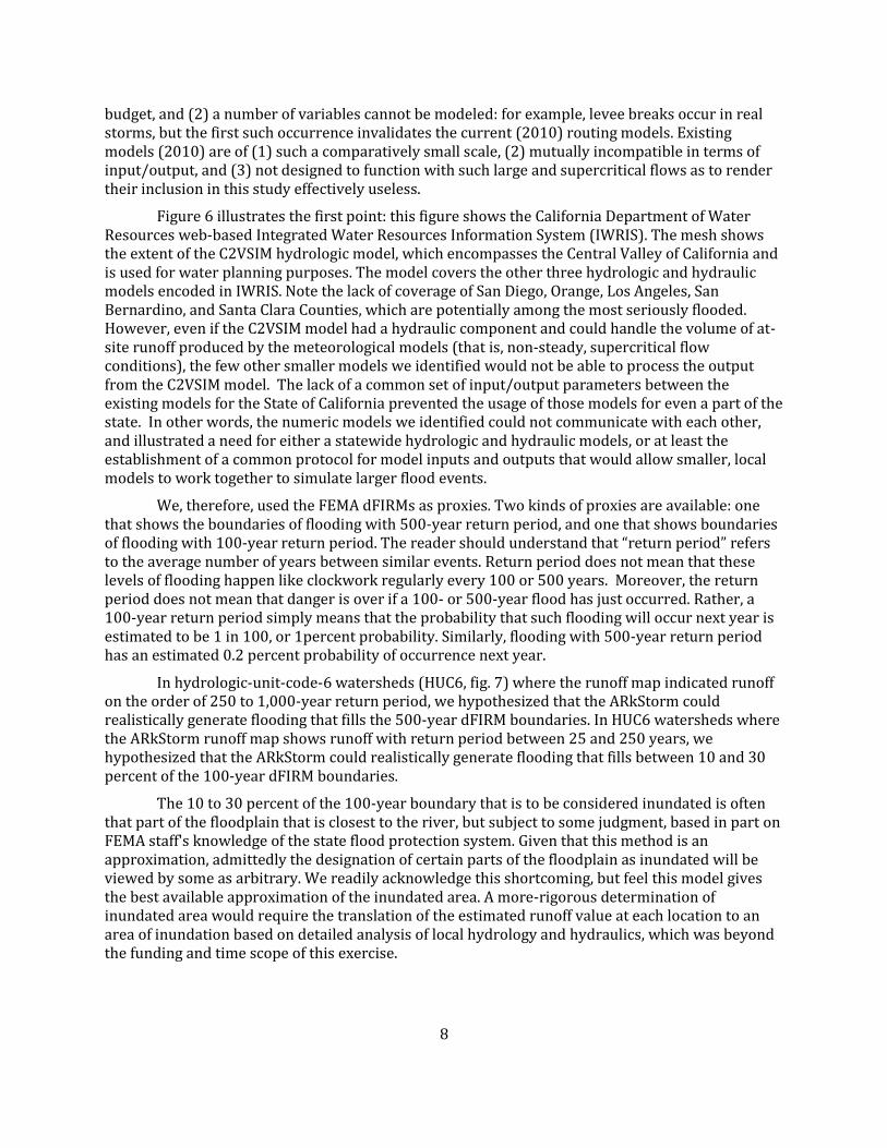
Figure 23. Route capacity on February 26, 2011. ....................................................................................... 30

Figure 24. Route capacity on April 27, 2011. ............................................................................................... 31

Figure 25. Route capacity on July 27, 2011. ................................................................................................ 32

Figure 26. Route capacity on January 27, 2012. ......................................................................................... 33

Figure 27. ARkStorm winds. Yellow indicates maximum windspeed in excess of 70 miles per hour. Red lines indicate electrical transmission lines. ....................................................................................... 36

Figure 28. Power plants (green diamonds) overlain with flooding (blue areas) in (a) San Francisco Bay Area, (b) Sacramento and Stockton, (c) Los Angeles and Orange Counties, and (d) San Diego. ............................................................................................................................................................................ 38

xii

Figure 29. Power restoration curves at a few key locations, showing percentage of customers capable of receiving power at selected times. ......................................................................................... 41

Figure 30. The larger water districts among the 324 federal, regional, state, and municipal water districts in California. Colors of districts varied to improve visibility. .................................................... 51

Figure 31. Major state water projects (modified from California Department of Water Resources, 2005). .................................................................................................................................................................. 52

Figure 32. Locations of California dams (yellow triangles). Only a fraction is for water-supply purposes. .......................................................................................................................................................... 53

Figure 33. Locations of 35,000 water wells in California (Department of Water Resources Integrated Water Resources Information System). .................................................................................. 54

Figure 34. Scenario water service restoration per county, showing percentage of customers with service at different times. .............................................................................................................................. 56

Figure 35. St. Francis Dam before (left) and after (right) collapse (both images: public domain). ... 58

Figure 36. South Fork Dam near Johnsontown, Pa., (left, image courtesy of Johnstown Area Heritage Association) and aftermath of the May 31,1889, Johnstown flood (right, public domain image). ............................................................................................................................................................... 58

Figure 37. Sacramento-San Joaquin Delta levee analysis zones. ......................................................... 61

Figure 38. Switch on wheels (left) and cellular on wheels (right) (Photograph taken by A. Tang, L & T Consulting)..................................................................................................................................................... 66

Figure 39. Microwave dish blown off the tower mount (left); flooded central office (right). (Kwasinski, 2006; public domain images) .................................................................................................... 67

Figure 40. Damage to fiber optic cables: flooding degraded transmission when water leaked into a splice (left); ground failure damaged a cable laid along a railbed that washed out (right). ............. 67

Figure 41. Early flooding along a levee (photograph taken by National Oceanic and Atmospheric Administration, date and location unknown). ............................................................................................ 71

Figure 42. Flooded vineyards, Guerneville, Calif., 2006, because of Russian River flooding (Photograph by A. Dubrowa for Federal Emergency Management Agency). ..................................... 73

Figure 43. State agricultural damages to annual and perennial crops and livestock. ....................... 79

Figure 44. County annual crop field repair costs and income loss. Shading of county indicates estimated dollar losses. Colors on pie charts indicate percentage of losses from each of the listed crops. ................................................................................................................................................................. 82

xiii

Figure 45. County perennial crop replacement and income loss (first year). Shading of county indicates estimated dollar losses. Colors on pie charts indicate percentage of losses from each of the listed crops. ............................................................................................................................................... 83

Figure 46. County perennial crop income loss (subsequent years). Shading of county indicates estimated dollar losses. Colors on pie charts indicate percentage of losses from each of the listed crops. ................................................................................................................................................................. 84

Figure 47. Livestock replacement cost. Shading of county indicates estimated dollar losses. Colors on pie charts indicate percentage of losses from each of the types of livestock listed. ...... 85

Figure 48. Time required to dewater 30 flooded Delta islands. .............................................................. 86

Figure 49. Sample HAZUS-MH flood vulnerability functions showing damage ratio for different types of single-family dwellings. .................................................................................................................. 90

Figure 50. ARkStorm hypothetical flooding in Sacramento. .................................................................... 92

Figure 51. ARkStorm hypothetical flooding in Stockton. .......................................................................... 92

Figure 52. ARkStorm hypothetical flooding in the San Jose area. ......................................................... 93

Figure 53. ARkStorm hypothetical flooding in Los Angeles and Orange Counties. ............................. 93

Figure 54. Basic wind speed map for California (American Society of Civil Engineers, 2006, figures 6-1) and adjoining states, showing zones where basic wind speed for design is 85 miles per hour (38 meters per second) and 90 miles per hour (40 meters per second). ............................................... 94

Figure 55. Fraction of building square footage affected by ARkStorm flooding for buildings in the occupancy classes agriculture, commercial, education, governmental, industrial, religion or nonprofit, and residential. .............................................................................................................................. 95

Figure 56. Contribution to $200 billion in flood-related building repairs (left), and $6 billion in wind-related building repairs (right) for buildings in the occupancy classes agriculture, commercial, education, governmental, industrial, religion or nonprofit, and residential. ........................................ 96

Figure 57. Estimates of number of people, per county, in areas flooded by the ARkStorm. Blue is fewer than 10,000 people, red is more than 400,000. ............................................................................ 104

Figure 58. Evacuation vulnerability index in northern inland region (Zone 1). ................................... 108

Figure 59. Evacuation vulnerability index in Delta counties (Zone 2). ................................................. 109

Figure 60. Evacuation vulnerability index in southern inland region (Zone 3). .................................. 110

Figure 61. Percentage of people in top two quantiles of the evacuation index relative to the total population (2009) by county. ........................................................................................................................ 111

xiv

Figure 62. Aggregate value added losses because of various components of storm damage for (A) flood damage. (B) wind damage (C) utility service interruptions (electricity, water, wastewater and telecommunications). (D) crop and livestock damage. (E) evacuation losses. ........................ 128

Figure 63. Employment and wage impacts of various components of storm damage for (A) flood damage, (B) wind damage, (C) utility service interruptions (electricity, water, wastewater and telecommunications), (D) crop and livestock damage, (E) evacuation losses. ................................. 135

Figure 64. TransNIEMO economic impact modeling framework. ........................................................ 140

Figure 65. National highway network volume change for southern California storm on day 3. ..... 143

Figure 66. National highway network volume change for northern California storm on day 14. ... 144

xv

Index of Tables

Table 1. Power restoration (percent of customers receiving power). ................................................. 40

Table 2. Wastewater treatment plants (WWTP) in scenario flooding areas, per county. ................ 43

Table 3. Sewer service restoration per county over time after the ARkStorm. .................................. 46

Table 4. Water service restoration per county over time. ...................................................................... 55

Table 5. Dewatering time of flooded Delta islands and tracts. ............................................................. 63

Table 6. Summary of Delta island repair costs and times...................................................................... 64

Table 7. Landline and internet network restoration showing percentage of customers with power service by date. ............................................................................................................................................... 68

Table 8. Cellular network restoration showing percentage of customers with power service by date. ................................................................................................................................................................... 69

Table 9. Field cleanup and repair cost assumptions. .............................................................................. 75

Table 10. Acres of significantly damaged agricultural lands. ................................................................ 78

Table 11 Statewide damages to annual crops for low, mid and high flood durations. ...................... 80

Table 12. Statewide damages to perennial crops over 5-year reestablishment. ............................... 80

Table 13. Statewide damages to livestock. ............................................................................................... 81

Table 14. ARkStorm property loss by county. ........................................................................................... 97

Table 15. National Flood Insurance Program flood insurance coverage. ......................................... 100

Table 16. Insured loss estimate for different levels of insurance. ...................................................... 101

Table 17. Estimates of county population living in flooded areas. ...................................................... 105

Table 18. Scaling of social indicators.for social vulnerability index. .................................................. 107

Table 19. Indicators for flood variables used in scaling of social vulnerability. ............................... 107

Table 20. Estimates, per county, of numbers of people in flood area. ................................................ 112

Table 21. Summary of Business Interruption double counting adjustments. .................................... 123

xvi

Table 22. Present discounted aggregate impact of various components of storm damage on value added. .............................................................................................................................................................. 129

Table 23. Present discounted sectoral impacts of flood losses. ......................................................... 136

Table 24. Summary of ARkStorm costs and business interruption. .................................................... 137

Table 25. Change in highway network truck travel time. ...................................................................... 142

Table 26. Change in highway network truck travel distance. .............................................................. 142

Table 27. Change in trucking costs. .......................................................................................................... 145

Table 28. Truck traffic economic impact. ................................................................................................ 146

Table 29. Generalized framework for U.S. disaster policy at the federal level. ................................ 153

Table 30. Generalized framework for U.S. disaster policy at the state level. ................................... 154

Table 31. Generalized framework for U.S. disaster policy at the local level. .................................... 155

Table 32. Generalized framework for U.S. disaster policy at the private level. ................................ 156

1

Introduction

Naming the ARkStorm. A California storm is known by the year in which the storm occurred. To equate the storm in a person’s mind requires some visceral knowledge of the event, or some understanding of history, meteorology, hydrology, engineering, or other relevant technical discipline. Even with that knowledge, the naming convention does not communicate the magnitude of the event. Therefore, the ARkStorm scenario was named so as to be independent of time, to acknowledge the meteorological phenomena behind most large storms on the U.S. West Coast, namely Atmospheric Rivers (ARs), and to provide some future scale to compare past and future events. The hypothetical scenario would be an Atmospheric River, AR with a value of 1,000 (k), or an ARkStorm.

The Multihazards Demonstration Project. The ARkStorm Scenario is the second major project of the U.S. Geological Survey (USGS) Multi-Hazards Demonstration Project (MHDP). The goal of the MHDP is to improve community resiliency to natural hazards through the application of science from a variety of disciplines. Early in the project, the MHDP gathered together decision makers and emergency managers in southern California and asked them what they wanted from science. Larry Collins, a Captain in the Los Angeles County Fire Department, Urban Search and Rescue, said:

“In California, the emergency services deal with disasters as a matter of course. It's the catastrophic events that push us to our limits. We look to science to help us better prepare for catastrophes. By preparing for catastrophes, we can deal with disasters that much better.”

There is much to learn from hypothetical catastrophes. To address southern California's catastrophic vulnerability to earthquake, the MHDP created the ShakeOut Earthquake Scenario. This scenario was the most comprehensive earthquake scenario ever devised, postulating a hypothetical magnitude 7.8 earthquake on the southern section of the San Andreas Fault. The scenario document (Jones and others, 2008) examined in detail the geophysical, physical, and social implications of a massive earthquake. This scenario was created by a team of more than 300 scientists and other experts. The ShakeOut scenario served as the centerpiece of the 2008 Great Southern California ShakeOut, the largest earthquake preparedness drill ever, with over 5.4 million participants. The ShakeOut is now an annual statewide event and the basis of the federal and state Catastrophic Earthquake Plan.

By postulating a hypothetical catastrophe, scientists and engineers can better examine the interdependencies in our social structure and infrastructure and expose the choke-points and vulnerabilities. In one of many examples in the ShakeOut scenario, we learned that all lifelines into and out of southern California cross the San Andreas Fault, most notably electrical transmission lines, oil and natural gas lines, water conveyance, telecommunications, highways, and railroads.

Everyone talks about The Big One, but what exactly does "The Big One" mean? Californians understand to some extent their vulnerabilities to earthquake. The idea of “the Big One” is ubiquitously understood to mean a very large earthquake that California will eventually experience. For many people this event exists in imagination extrapolated from movies and possibly from personal experience in damaging earthquakes they have actually lived through, such as the 1989 Loma Prieta or 1994 Northridge earthquake. Having personal experience and an awareness that a much larger earthquake has and will occur, helps people understand the need for earthquake risk mitigation. Both elements—personal experience and a cinematic or other basis for extrapolation—are largely missing from the public’s understanding of catastrophic winter storms. Storms in the public’s own experience have caused inconvenience but not major societal impacts.

2

So although potentially catastrophic storms have occurred in the past, these storms are beyond living memory, and so are less real to many people. Storms also are less sudden, less dramatic, and thus loom smaller than earthquakes do in the imagination of risk. But the evidence shows these storms do pose a real risk to California, in some ways far greater than that of earthquakes. One sequence occurred almost 150 years ago.

Winter storms of 1861-1862. Beginning in early December 1861 and continuing into early 1862, an extreme series of storms lasting 45 days struck California. The storms caused severe flooding, turning the Sacramento Valley into an inland sea, forcing the state capitol to be moved temporarily from Sacramento to San Francisco, and requiring Governor Leland Stanford to take a rowboat to his inauguration. William Brewer, author of "Up and down California," wrote on January 19, 1862, "The great central valley of the state is under water-the Sacramento and San Joaquin valleys-a region 250 to 300 miles long and an average of at least twenty miles wide, or probably three to three and a half millions of acres!"

The 1861-62 series of storms were the largest and longest California storms in the historic record, but were probably not the worst California has experienced. Geological evidence indicates that floods that occurred before Europeans arrived were bigger. Scientists looking at the thickness of sediment layers collected offshore in the Santa Barbara and San Francisco Bay areas have found geologic evidence of megastorms that occurred in the years 212, 440, 603, 1029, 1418, and 1605, coinciding with climatological events that were happening elsewhere in the world. There is no scientific evidence to suggest that such extreme storms could not happen again.

To demonstrate and prepare people for the risks associated with an event analogous to the 1861-62 series of storms, the MHDP began the ARkStorm scenario on October 28, 2008. As with the ShakeOut earthquake scenario, the MHDP and its many contributing scientists created a hypothetical, but scientifically defensible storm scenario and then in detail examined the risks associated with that storm, including the potential impact on our buildings, infrastructure, water supply, transportation, agriculture, environment, and economy.

About the storms of 1861-62, Marcia Eymann, History

Manager, Center for Sacramento History, writes:

Some capital-city residents opted to ignore the obvious danger

and attempted to enjoy the perceived novelty of the event.

Historians Thompson and West write that “every balcony was

crowded with spectators, and mirth and hilarity prevailed.

However hard these citizens tried to enjoy the flood, they soon

found it difficult to do so in the face of so much destruction.

The levees remained intact, trapping flood waters inside the

city. Residents were subject to hurricane-force winds and ice-

cold, muddy water. The chain gang was charged with the

dangerous task of breaching the R Street levee to relieve

Sacramento of the excess water. Once it was breached, the

force of the rushing water was so great that it took twenty-five

homes with it, some of which were two stories tall. Sacramento

remained under water for three months while four hundred

families were left homeless and five thousand people were in

need of aid.

San Francisco preacher S.C. Thrall explained that the great

storm’s visitation to California was simply God’s way of

punishing the nation for the sins of greed and pride. In early

1862 he proclaimed, “He who visited the nation with war, has

smitten us with flood ... That this calamity is our part of the

punishment of national sin seems especially evident from the

fact that the visitation is so precisely coincident with the portion

of our inhabited territory which has escaped the consequences

of war.”

In southern California lakes were formed in the Mojave Desert

and the Los Angeles Basin. The Santa Ana River tripled its

highest-ever estimated discharge, cutting arroyos into the

southern California landscape and obliterating the ironically

named Agua Mansa (Smooth Water), then the largest

community between New Mexico and Los Angeles. The storms

wiped out nearly a third of the taxable land in California, leaving

the State bankrupt.

3

This is the ARkStorm. This document summarizes the environmental effects, physical damages, economic and other losses in California as a result of the hypothetical flooding and high winds associated with the ARkStorm scenario. ARkStorm is an emergency planning scenario associated with a hypothetical severe winter storm striking California, imagined to begin on January 19, 2011. The scenario was designed by a collaborative group led by the U.S. Geological Survey, California Geological Survey, and others, under the authority of the U.S. Geological Survey Multi-Hazards Demonstration Project for Southern California.

ARkStorm Meteorology

We begin with a brief history of extreme weather in California, touching on the historic precedent supporting the ARkStorm realism, especially the 1861-1862 severe storms that caused inundation throughout northern and southern California (fig. 1). These storms, and indeed most severe precipitation in California, were probably the result of a phenomenon termed atmospheric rivers, jets of warm moist air that originate over the mid-latitude north Pacific Ocean and transport that moisture to California where much of the moisture turns to rain and snow that falls on the state (fig. 2; http://www.noaanews.noaa.gov/stories2005/s2529.htm)

Figure 1. K Street, Sacramento, looking east, in January or February 1862. (Photographers Lawrence and Houseworth, The Bancroft Library Pictorial Collection, University of California, Berkeley)

http://www.noaanews.noaa.gov/stories2005/s2529.htm�

4

Figure 2. This map of the Pacific region shows an Atmospheric River originating over the central Pacific on February 16, 2004, indicated by high (green) vertically integrated water-vapor contents, in grams per square centimeter of water vapor, in the atmosphere extending from around Hawaii to the central California coast near the town of Cazadero (CZD).

These atmospheric rivers, the meteorological conditions that produce them, and the resulting precipitation and winds that affect California, can be simulated by using computer models. These models are based on observations of atmospheric conditions, plus laws of fluid dynamics and thermodynamics that allow us to fill in the gaps between observations.

This technique was done for ARkStorm. The modeling was led by Mike Dettinger and Marty Ralph of the USGS and National Oceanic Atmospheric Administration (NOAA), respectively, along with a team of 13 others from Scripps Institution of Oceanography, the National Weather Service, the California Extreme Precipitation Symposium, Golden Gate Weather, San Francisco State University, the Western Regional Climate Center, and the California Department of Water Resources. For technical details of this modeling, Dettinger and others have a paper in progress (M. Dettinger, written commun., 2009).

The modelers employed the Global Climate Model (GCM)—a computer model that depicts the climate of the world over time at a fairly large scale, on the order of 150 kilometer (km) horizontal grid—and nested within a portion of the model over California they used a detailed climate model termed the Weather Research and Forecasting (WRF) model, which depicts weather in nested domains each resolving smaller scales (fig. 3). From innermost to outermost boxes, the grid spacings are 2 km (black box), 6 km (black), 18 km (blue) and 54 km (red) (Dettinger and others written commun., 2009). Encoding the laws of fluid dynamics and thermodynamics in

5

equations that operate on meteorological parameters such as temperature, pressure, moisture content, and windspeed, the model calculates these parameter values at each grid point in the model and at each time step (here, about 30-second increments) during whatever duration is of interest. One can record all the parameter values at each grid point and time step, but for practical purposes, it is generally only necessary to record certain key parameters at larger time steps for later use, such as to make the maps shown later.

Figure 3. Weather Research and Forecasting (WRF) model domains used in simulations of ARkStorm meteorology, with nested model domains indicated by boxes and the topography resolved by the grids in each domain indicated by contours. Grid spacings are 2 km in smaller black box, 6 km in larger black box, 18 km in blue area, and 54 km in red area.

To use the GCM and WRF models requires one to establish what are called boundary conditions, meaning the constraints or inputs at the temporal and spatial boundaries of the model. To have any faith in the boundary conditions and the model results, it also helps to have some actual physical observations with which one can compare the model's output. Because the 1861-1862 storm occurred at a time before extensive detailed and generally reliable measurement of precipitation, barometric pressure, and wind speeds, we did not attempt to model the 1861-1862 storms directly, which would have required too many arbitrary assumptions, and instead simulated a repetition of two actual storms in recent history for which boundary conditions are known. In particular, the ARkStorm is a hybrid of a storm that struck southern California from January 19-27, 1969, followed without delay or interruption by a repetition of the storms that struck northern California from February 8-20, 1986, (fig. 4). That is to say, the GCM and WRF models were used to calculate and record the windspeed, barometric pressure, precipitation, and other weather parameters at each grid point on an hourly basis for 217 hours of a hypothetical storm that merges these two real events. The ARkStorm adds to these two storms a 24-hour period at the height of the

6

January 1969 storm in which the storm is imagined to stall, so as to produce a sufficient amount of precipitation to approximately match the limited observations of 1861-1862.

Figure 4. ARkStorm stitched-storm calendar, with moderately wet conditions of autumn and early winter “preconditioning” the watersheds of California for rapid flood generation indicated by blue shading, followed by the two intense-storm periods that were combined to make up the ARkStorm scenario indicated in red shading. These calendars represent actual storms of 1969 and 1986, which provided the basis for the ARkStorm modeling.

Using the modeled ARkStorm precipitation and temperatures, along with a macro-scale hydrology model termed the variable infiltration capacity model, the research team estimated the runoff generated by the ARkStorm, on an approximately 8-km grid throughout most of the state. Here, runoff means the rainfall that neither seeps into the ground or flora nor evaporates, but instead runs overland toward streams and ultimately the Pacific Ocean.

The meteorology team compared this modeled ARkStorm runoff with extreme-value statistics of runoff generated by the model for water years 1916-2003. In particular, the team fit a type-III log-Pearson parametric distribution to the yearly maximum 1- 3- and 7-day runoff volume in each grid cell, by using the statistics of these 87 years of simulation. One can compare the ARkStorm runoffs to this distribution to find the approximate return period of ARkStorm runoff in each grid cell. By return period, we mean the average number of years one would have to wait to observe storms generating at least that level of runoff. The calculation requires one to assume that the period 1916-2003 is representative of the future (reasonable, although climate change makes the assumption increasingly questionable the farther into the future we project), and that the type-

7

III log-Pearson parametric distribution is a reasonable approximation of the true probability distribution of runoff volume (a common assumption). Given this model, as shown in figure 5, ARkStorm produces runoff with a return period that varies between 10 years and 1,000 years, depending on location, relative to an historic simulation of water years 1916-2003 (Dettinger and others, written commun., 2009). Bear in mind that a storm can produce very high, rare runoff in one location and very low, commonly observed runoff in another, and no directly produced runoff in a third, so the runoff return period varies spatially for any given storm.

Figure 5. For locations around California, colors depict recurrence intervals in years of maximum 3-day runoff during the ARkStorm scenario.

FLOODING

The runoff map was interpreted to produce a map of flooding. The map was generated by a team led by Justin Ferris of the USGS, with 14 others from the USGS, University of Colorado, Federal Emergency Management Agency (FEMA), the Michael Baker Corporation, California Department of Water Resources, and NOAA. Note that the FEMA and Michael Baker Corporation representatives are currently responsible (at least during the period October 2009-April 2010) for accrediting levees in California for purposes of establishing digital flood information rate maps (dFIRMs).

Although a statewide analysis of the expected runoff is estimated by the meteorology modeling effort, this runoff is calculated on an 8 km grid, which is insufficient to estimate the runoff at specific locations with a great level of confidence. Ideally we would have performed a detailed statewide hydrological and hydraulic analysis for the storm to estimate flooding. However, there are two key challenges to such an approach that we could not overcome during this project: (1) no such model currently (2010) exists, and we could not create one within the available time and

8

budget, and (2) a number of variables cannot be modeled: for example, levee breaks occur in real storms, but the first such occurrence invalidates the current (2010) routing models. Existing models (2010) are of (1) such a comparatively small scale, (2) mutually incompatible in terms of input/output, and (3) not designed to function with such large and supercritical flows as to render their inclusion in this study effectively useless.

Figure 6 illustrates the first point: this figure shows the California Department of Water Resources web-based Integrated Water Resources Information System (IWRIS). The mesh shows the extent of the C2VSIM hydrologic model, which encompasses the Central Valley of California and is used for water planning purposes. The model covers the other three hydrologic and hydraulic models encoded in IWRIS. Note the lack of coverage of San Diego, Orange, Los Angeles, San Bernardino, and Santa Clara Counties, which are potentially among the most seriously flooded. However, even if the C2VSIM model had a hydraulic component and could handle the volume of at-site runoff produced by the meteorological models (that is, non-steady, supercritical flow conditions), the few other smaller models we identified would not be able to process the output from the C2VSIM model. The lack of a common set of input/output parameters between the existing models for the State of California prevented the usage of those models for even a part of the state. In other words, the numeric models we identified could not communicate with each other, and illustrated a need for either a statewide hydrologic and hydraulic models, or at least the establishment of a common protocol for model inputs and outputs that would allow smaller, local models to work together to simulate larger flood events.

We, therefore, used the FEMA dFIRMs as proxies. Two kinds of proxies are available: one that shows the boundaries of flooding with 500-year return period, and one that shows boundaries of flooding with 100-year return period. The reader should understand that “return period” refers to the average number of years between similar events. Return period does not mean that these levels of flooding happen like clockwork regularly every 100 or 500 years. Moreover, the return period does not mean that danger is over if a 100- or 500-year flood has just occurred. Rather, a 100-year return period simply means that the probability that such flooding will occur next year is estimated to be 1 in 100, or 1percent probability. Similarly, flooding with 500-year return period has an estimated 0.2 percent probability of occurrence next year.

In hydrologic-unit-code-6 watersheds (HUC6, fig. 7) where the runoff map indicated runoff on the order of 250 to 1,000-year return period, we hypothesized that the ARkStorm could realistically generate flooding that fills the 500-year dFIRM boundaries. In HUC6 watersheds where the ARkStorm runoff map shows runoff with return period between 25 and 250 years, we hypothesized that the ARkStorm could realistically generate flooding that fills between 10 and 30 percent of the 100-year dFIRM boundaries.

The 10 to 30 percent of the 100-year boundary that is to be considered inundated is often that part of the floodplain that is closest to the river, but subject to some judgment, based in part on FEMA staff's knowledge of the state flood protection system. Given that this method is an approximation, admittedly the designation of certain parts of the floodplain as inundated will be viewed by some as arbitrary. We readily acknowledge this shortcoming, but feel this model gives the best available approximation of the inundated area. A more-rigorous determination of inundated area would require the translation of the estimated runoff value at each location to an area of inundation based on detailed analysis of local hydrology and hydraulics, which was beyond the funding and time scope of this exercise.

9

Figure 6. This snapshot of available flood models shows that various models cover the Central Valley (gridded area) but not the rest of the state (California Department of Water Resources, 2010a).

We added the 500-year dFIRM floodplains in HUC6 watersheds to those areas with approximately 500-year runoff, producing the flooding map shown in figure 8. This and other Google Earth maps were made available for interactive inspection by project participants. FEMA and USGS personnel reviewed the resulting map and found it to be realistic.

Other experts disagree with the flooding map we generated, one particularly with regard to flooding in Sacramento, another with regard to flooding in the California Delta. We found their concerns to be valid, especially with regard to the need for more thorough hydrologic and hydraulic analyses, though as discussed earlier such analyses were not practical for this study. However, after considering the particulars of their concerns, which are not detailed here, we judged their concerns valid but not compelling enough to invalidate the ARkStorm flood map that we had previously generated.

10

After the areas of inundation were decided upon, the flooding panel applied its knowledge of the local hydrology and hydraulics to estimate, for each HUC6 watershed, peak depth and duration of flooding (fig. 7). The panelists split two watersheds (Lower Sacramento and San Joaquin) into 3 smaller zones each, and estimated depth and duration for each of the 6 zones. Flood extents, depths, and durations were documented in ARCGIS and Google Earth KMZ files and other media, and used in later discussions and analyses

Figure 7. Hydrologic Unit Code 6 watershed boundaries, with ARkStorm flooding parameter values, depth of flooding and length of time flooded.

11

Figure 8. Blue areas indicate ARkStorm flooding as projected by models used in the scenario.

WINDSPEED

The windspeed time series generated by using the Weather Research and Forecasting (WRF) model were processed as follows. The time series contain the 30-second average windspeed at the beginning of each hour, at 10-meter elevation, at each of 59,580 grid points, over a 9-day period. For each grid point, the maximum value of the hourly samples is interpreted as the maximum 30-second gust velocity at that site. (The calculated maximum probably occurred during the hour.) Most structures tend to be sensitive to shorter-duration and more-intense gusts, therefore, we multiplied the maximum 30-second gust velocity by the ratio of 3-second gusts to 30-

12

second gusts, based on the work of Vickery and Skerlj (2005, fig 2). This ratio is approximately 1.18. The results were converted into Google Earth (KMZ) files as shown in figure 9. The figure shows peak gusts of 50 mph throughout much of the state, reaching as high 125 mph in mountainous regions.

Figure 9. ARkStorm peak 10-meter elevation, 3-second gust wind speeds.

Coastal Inundation

The time-series of sea surface pressure, wind speed, and wind direction generated by the ARkStorm meteorological model provided boundary conditions for a complex, process-based numerical modeling system for simulating the impact to the Southern California coast, stretching 473 km from the Mexican border to Point Conception (fig. 10; KMZ project file available on request). The objective was to use a physics-based approach to identify the location and magnitude of the potential coastal hazards during the simulated storm. The Coastal Storm Modeling System (CoSMoS) was developed for the ARkStorm to incorporate atmospheric information (that is, wind

13

and pressure fields) with a suite of state-of-the-art physical process models (that is, tide, surge, and wave) to enable detailed prediction of currents, wave height, wave runup, and total water levels for mapping the distribution of coastal flooding, inundation, erosion, and cliff failure. The Google Earth-based product output of CoSMoS is designed to provide emergency planners and coastal managers with critical information to increase public safety and mitigate damage associated with powerful coastal storms. Further details of the CoSMoS framework can be found in Barnard and others (2009). The Digital Elevation Model (DEM) serving as the morphological boundary condition is described in Barnard and others (2009).

Figure 10. Extent of the CoSMoS model applied to the ARkStorm scenario. See Barnard and others (2009) for details and additional maps.

Findings. Figure 10 highlights locations of moderate and high wave damage potential (yellow and red squares, respectively) and moderate and high cliff failure potential (yellow and red triangles). The summary map shows that severe wave damage potential is predicted on the mostly west-facing beaches in Los Angeles and northern San Diego Counties, and the oil platforms in the western part of the Santa Barbara Channel. The coastal infrastructure that appears most at risk of severe wave damage includes the Manhattan, Hermosa, Venice and Imperial Beach piers, as well as coastal structures (for example, groins, jetties, seawalls) in the Los Angeles International Airport (LAX) region, and along Highway 1 in northern San Diego County. Sewage infrastructure near LAX (for example, Hyperion Treatment Plant) also appears vulnerable. Coastal flooding, resulting from the combined factors of tidal elevation, storm surge, and wave set-up, is most extensive and potentially damaging for southern Oxnard and Mugu Naval Air Station, Marina Del Rey, the Ports of Los Angeles and Long Beach (fig. 11), Seal Beach (fig.12), Del Mar (note: race track flooding), Mission Bay (fig.13) and Coronado and Imperial Beaches (fig. 14). Drastic shoreline change (beach erosion) induced by the ARkStorm conditions could lead to significant damage to public and private infrastructure, including the following regions: Imperial Beach, La Jolla, Del Mar, Solana Beach,

14

Carlsbad, Malibu, Santa Clara River mouth (for example, McGrath State Park), Rincon Parkway, Carpinteria, and Isla Vista (for example, University of California at Santa Barbara). The cliff failure pilot project in Santa Barbara only identifies a few sites with major cliff failure potential, but one of those sites is immediately adjacent to the Summerland Water Treatment Facility.

Figure 11. CoSMoS-estimated coastal inundation at the Ports of Los Angeles and Long Beach.

Figure 12. CoSMoS-estimated coastal inundation at Seal Beach.

15

Figure 13. CoSMoS-estimated coastal inundation at Mission Bay, San Diego.

Figure 14. CoSMoS-estimated coastal inundation at Coronado and Imperial Beaches.

16

RESEARCH NEEDS RELATED TO COASTAL INUNDATION

Elevation data. The model relies on high-resolution, coastal elevation data (LIDAR and multibeam bathymetry). The available data could be brought up to date and expanded to cover a greater area.

Model development. We believe it would be beneficial to test and validate physical process models for the U.S. West Coast. It would also be beneficial to develop integrated modeling systems for easily assimilating atmospheric forcing data.

Landsliding

Landslides in California, triggered by historic storms, have caused hundreds of millions of dollars in damage and numerous casualties. Buildings, roads, pipelines, and other structures have been damaged by being entrained in, deformed by or as a result of the inertial impact of material flowing or sliding downslope. Landslides can be classified by the type of earth material moving and by the mode of movement (Cruden and Varnes 1996). For the ARkStorm scenario, we focus on two general modes of landsliding: (1) Large, deep-seated, slow-moving landslides usually classified as either rock slides or earth flows; and (2) Small, shallower, fast-moving landslides, usually classified as debris slides or debris flows. Figures 15 and 16 illustrate these end-member divisions of landslides. The simple division of landslides into two end member types also can be applied to landslide damage and risk, because large, slow, deep-seated landslide cause damage to structures and infrastructure while small, shallow, fast-moving landslides often threaten lives.

To characterize the potential for landslides in the ARkStorm scenario, we developed two maps of landslide susceptibility for California, one for deep-seated landslides and the other for shallow slides. We evaluated susceptibility to larger, deep landslides by combining estimates of rock strength with slope. Hundreds of mapped geologic units from numerous sources were generalized into three rock strength classes according to the approach presented by Wieczorek and others (1985). Three rock strength units, which we call hard rock, weak rock, and soil, are combined with slope to derive 10 landslide susceptibility classes following the procedures developed by Ponti and others (2008) for the ShakeOut earthquake scenario. Locations where past landslides have occurred are assigned the lowest value of rock strength. The resulting map of susceptibility to deep-seated landslides (fig. 17) shows those areas most likely to experience deep-seated landslide damage in the ARkStorm.

There are no established techniques to estimate the number of shallow landslides a storm will trigger across broad regions. Shallow landslides tend to occur during the most intense rainfalls of the storm in steep convergent areas, and involve failure of the soil and weathered bedrock layers. A fraction of these failures mobilize as debris flows, mixtures of soil, water, and rock, that sweep down steep valleys at high velocities and destroy homes and infrastructure with little warning. Historical accounts indicate that storms with more intense, longer lasting rainfalls trigger more shallow landslides. Shallow landslide susceptibility models, however, vastly overpredict the number of failures actually triggered by historic storms, and do not allow us to forecast the number of shallow landslides for a given storm. To evaluate susceptibility to shallow landsliding for the ARkStorm simulation, shallow landslide abundance was assumed to increase with rainfall intensity, duration, and number of unstable model cells in topographically-based landslide susceptibility models. Rainfall intensity and duration were calculated from hourly rainfall records, and the shallow landslide susceptibility model SHALSTAB (Dietrich and others, 1995; Dietrich and Montgomery, 1998; Dietrich and others, 2001) was used to estimate the number of unstable cells in

17

a 10-m DEM. Digital maps of historic shallow landslides in southern California (Santa Paula and Sunland quadrangles) and northern California (Montara Mountain Quadrangle) were used to locate landslide initiation points, and to calculate the fraction of unstable cells that actually failed for a given rainfall metric. Landslide abundance for southern California sites was found to increase as a power law function of 6-hour rainfall intensity. The hourly rainfall data from the ARkStorm simulation was then used to calculate the maximum 6-hour rainfall intensities across the Southern California landscape, which was then used to estimate the abundance of shallow landslides that would likely be generated by the ARkStorm simulation (fig. 18).

Landslides on hill slopes damage buildings and other structures on those slopes, and in some circumstances can cause significant damage beyond the hills. Alluvial fans, which underlie many urban and suburban areas of California, are built up by repeated deposits transported from the mountains in floods. A significant part of those deposits may be the result of debris flows. Projecting the run-out areas that could be impacted by debris flows is a developing science. Scientists with the California Geological Survey are preparing maps showing areas where relatively recent alluvial fan deposits are found, and so could be subject to alluvial fan flooding. This includes debris flows and more conventional flood flows and gives a maximum extent of the potential hazard. The USGS has developed another approach to estimate the volume of material that could be mobilized as debris flows in rainfall following a fire and how far material could flow down channels. This approach gives a much more detailed look at a specific aspect of the debris flow hazard, but is unavailable to model debris flows over an area of the size that could be impacted by the ARkStorm. Although we have not attempted to estimate the amount of damage that could result from debris flow runout and alluvial fan flooding, the evaluations prepared for the ARkStorm scenario show the areas potentially impacted by this hazard.

Having established statewide susceptibility maps for deep-seated and shallow landslides, this study considered the risk these potential landslides pose to the constructed environment. However, landslide damage cost information is very limited, and this part of the ARkStorm evaluation was projected from a few small datasets. The most detailed and complete available data on landslide damage to buildings was gathered by the City of Los Angeles following the 1978 storms. The damage cost reported in that dataset is estimated for each locality, and the type of landslide involved is described. This dataset shows the majority of the building damage from “surface slump” or “rotation,” with a relatively small fraction due to “mudflow.” Though limited, these data were extrapolated to the rest of the state and compared with susceptibility maps for deep-seated landslides.

The susceptibility map for deep-seated landslides was generalized to give a single value of susceptibility for each census tract. A “loss ratio” was calculated for each census track as the cost of landslide damage from the 1978 storms divided by the value of light wood frame structures within the census tract. Using the median susceptibility for each census tract provides three general categories of damage:(1) tracts with a median susceptibility of 0 to 3 have no landslide damage, (2) tracts with median susceptibility of 5 or 6 have loss ratios of about 0.016 percent, (3) and tracts with median susceptibility of 7 or above have loss ratios of 0.096 percent. The susceptibility map was converted to a landslide loss ratio map by using these values, (fig. 19). These loss ratios are for the average storm intensity and landslide vulnerability of Los Angeles in 1978; projected statewide. Generalization to other storm intensities is possible by using data from the San Francisco Bay Area. Damage from the 1982 storm in Santa Cruz County was over 3 times our loss ratio projection from the 1978 data, while damage in Sonoma County was only 5 percent of our projection. This probably reflects regional variation in the intensity of the 1982 storm, which had a recurrence interval of over 100 years in Santa Cruz, but only about 10 years in Sonoma County. Using this tentative

18

relationship, the ARkStorm is estimated to cause at least three times our projections of building damage from the 1978 data, similar to the relatively rare, very intense 1982 storm in Santa Cruz County.

Data on landslide damage to roads, pipelines, and other infrastructure is similarly sparse and inconsistent. The relatively complete records kept by California Department of Transportation (Caltrans) over the past decade give some perspective on the cost of landslides to roads. Based on records of “emergency opening” costs, Caltrans spends $20-40 million on landslide repairs in a typical year. In wet years the cost jumps to about $150 million. Projecting from these data to the amount of rainfall in the ARkStorm suggests costs of about $300 million. In addition to “emergency opening,” Caltrans plans and budgets for long-term landslide repair projects. The average cost of these projects over the past decade has been about equal to the cost of “emergency opening”. Landslide damage to local roads, pipelines, electric transmission lines and other infrastructure has been greater than the damage to state highways in past storms (Crovelli and Coe, 2009).

Despite the major data gaps and the broad generalizations that resulted, our best estimate is that the ARkStorm could cause tens of thousands of landslides, the vast majority of them debris flows, and cost on the order of $3 billion. This estimate includes about $1 billion in damage to private property, $1 billion to state highways, and $1 billion to other infrastructure. Costs because of debris flow runout, which cannot be estimated at this time, and indirect costs because of disruption of infrastructure and other indirect damage will multiply these direct losses.

Figure 15. Categories of landslide treated by ARkStorm (Wills and others, 2001 modified after Varnes, 1958 and Colorado Geological Survey, 1988)

19

Figure 16. Deep-seated landslide in Ventura Calif., January 2005 (left, photo credit: J. Stock, USGS), and 1982 debris flow in Pacifica, Calif., that killed 3 (right, photo courtesy of Woodward Clyde Consultants).

20

Figure 17. Deep-seated Landslide Susceptibility Map of California. Black lines denote county boundaries. Higher numbers and hotter colors indicate greater susceptibility to deep-seated landslides.

21

Figure 18. Quaternary, Pliocene, and Miocene sedimentary rocks (hachured area) superimposed on the forecast for landslide abundance resulting from the ARkStorm. Cells in the hachured area have rock types similar to the calibration area at Santa Paula. Cells outside these zones likely overestimate the number of landslides because (1) rock units produce stronger soils and (2) different processes (for example, rock fall) dominate erosion. Gray areas have no unstable cells in 10-meter data. Calibration (Santa Paula) and test (Sunland) areas shown by white polygons.

22

Figure 19. Deep-seated Landslide susceptibility expressed as the median value for each census tract, which can be related to loss ratio for that tract.

RESEARCH NEEDS RELATED TO LANDSLIDING

Our ability to understand and model landsliding and its consequences would benefit from:

Accurate digital mapping of historic landslides;

Accurate digital mapping of historic and pre-historic storm damage; and

Methods for estimating damage from debris-flow runout and alluvial fan flooding.

23

Three Approaches to Estimating Damage

To help inform our damage estimates, we compiled an extensive database of historic storm impacts in California, including summaries of news reports and newspaper images from 1861-1862, 1938, 1969, 1986, and 1997. Many of these reports and images were geolocated and placed in Google Earth files for interactive examination. The database is too extensive to copy in this report; the database was made available for examination by ARkStorm panelists and scenario developers.

We estimated physical damages in the ARkStorm scenario by three different approaches. To produce a realistic outcome at the aggregate societal level, we employed the data and methods of the FEMA flagship emergency-planning software HAZUS-MH. To examine the effects of the ARkStorm on lifelines such as the highway network, power, and water, a series of 12 panel discussions were held with engineers, operators, and emergency planners from the various lifelines at risk. The panel participants were presented with the meteorological and flooding inputs, and offered their judgments about the resulting damage and restoration efforts that they would undertake if ARkStorm really occurred. Finally, three studies were performed by individual experts on topics requiring highly specialized knowledge: demand surge, telecommunications, and insurance.

To be clear: we did not apply all three approaches to each type of asset at risk. Only one approach was used for each particular kind of asset: lifelines damage was estimated based only on the expert opinion of the lifeline operators themselves, building damage was estimated by using only the HAZUS flood methodology, and three consultant reports were commissioned on specific topics. We begin by presenting lifeline panel findings, then present HAZUS-based property loss estimates, and conclude with the special studies.

Lifeline Panel Process

In January and February 2010, scientists and engineers developing the ARkStorm scenario convened 12 half-day meetings in Pasadena, Sacramento, Menlo Park, and San Francisco with officials of 43 federal, state, local, and private agencies, utilities, and universities listed in the Acknowledgments section of this report. They were from departments of transportation, water and wastewater service providers, power utilities, public-health and public-safety agencies, and entities that own, maintain, or regulate dams and levees.

Panels were convened on four topics: roads and highways; dams and levees; power; and water and wastewater. Each topic was addressed by a different panel in each of these general locations: Pasadena (for participants based in southern California), Menlo Park and San Francisco (for the San Francisco Bay Area), and Sacramento (for Central Valley participants). We sent 229 invitations; approximately 85 people attended the panel discussions.

The purpose of the lifeline panels was fourfold: (1) to educate lifeline operators of the potential for and impacts of an event like an ARkStorm, and thus indirectly to stimulate discussion within their organization about enhancing disaster resiliency; (2) to gather panelists’ expert opinion as to the physical damage of the hypothetical storm and other impacts to the facilities they operate; (3) to gather their expert opinion about the time it realistically could take to restore their facilities, considering among other things lifeline interaction; and (4) to identify important research needs highlighted by the ARkStorm.

Participants were invited by email and follow-up phone calls, generally beginning 2 to 4 weeks in advance. The invitations also included a brief abstract summarizing the ARkStorm

24

scenario and URL and credentials for downloading the Google Earth maps of windspeed, flooding, and historic impacts.

Each meeting generally followed the same agenda: 1.5 hours in which the ARkStorm development team summarized the material presented above, plus findings of panels that had already met, followed by 2.5 hours in which the group discussed the assets exposed to damage, the agents of damage, a realistic damage scenario, a realistic restoration scenario, and a discussion of opportunities to enhance resiliency either by strengthening facilities or by better responding to damage so as to minimize the negative impacts of damage. We made audio recordings and took notes of the discussion. After the panel meetings, we synthesized the notes and filled gaps through literature searches and additional analysis, as discussed below.

A note regarding methodology: We considered but dismissed the notion of following a formal process for eliciting expert opinion such as a Delphi Process (Dalkey and others, 1970). Considering the quantity of information we needed, such a process appeared likely to be excessively time consuming and likely to be off-putting to panelists. An important advantage of the Delphi process is that it prevents a few individuals from dominating the discussion. On the other hand, the same end can be achieved if the moderator is trained in group communication and deliberately seeks discussion from all panelists, including the quieter ones. Our less-formal approach seemed more suited to meet our objectives, particularly of stimulating discussion with panelists’ organizations, although this approach may lack scientific rigor.

Highway Damage

HIGHWAY FACILITIES AND SOURCES OF DAMAGE

The state of California has more than 50,000 miles of highway and freeway lanes, managed by Caltrans. According to the National Bridge Inventory, there are more than 23,000 bridges in the state. The primary perils to highways are landslides either burying or undermining them; floods inundating them; and clogged culverts causing flooding and erosion where the water washes over the roadway and onto the soil beyond. The primary causes of bridge damage in severe winter storms are scour undermining the foundations of bridge piers or abutments and hydrodynamic pressure at the upstream edge of the bridge superstructure (the girders, driving surface, and crash barriers).

HIGHWAY DAMAGE AND RESTORATION SCENARIO

Since this slope-stability research was ongoing at the time of the panels, we applied the judgment of ARkStorm research staff and of Caltrans panel participants to select locations where landslides bury or undermine roadways, or block culverts and cause flooding and erosion. Likewise, because streamflows were not calculated at each bridge location, we applied judgment to select bridges to hypothesize as damaged by scour at the substructure or hydrodynamic pressure on the superstructure. Locations of inundation were identified by overlaying the flooding map on the roadway network. The resulting hypothetical damage is mapped in figure 20, which distinguishes highway impacts as resulting from either: (1) debris flow; (2) flooding, (3) both flooding and erosion, and (4) landsliding.

25

Restoration time was estimated depending on the type and extent of damage. Hypothesized duration of flooding dictates how long roads are inundated and impassible. Debris flows can be cleared relatively quickly, within hours of equipment and repair crews arriving. However, on routes with large numbers of debris flows the time to clear each flow adds up, and the importance of the route—how much traffic normally carried and the availability of alternate routes—matters greatly to how routes are prioritized for clearing. Bridges with severe foundation damage or displaced spans can take months to repair or replace. Roads over deep-seated landslides can be partially restored quickly by regrading and reducing the speed limit, but permanent repair could take months.

With these considerations in mind, the highway panels estimated the number of days required restore each route to 25 percent, 75 percent and 90 percent capacity, beginning after the peak of each storm, that is, January 27, 2011, in southern California, and February 9, 2011, in northern California. For present purposes, southern California comprises counties including and south of Santa Barbara, Ventura, Los Angeles, and San Bernardino. Northern California comprises all the counties north of these counties.

26

Figure 20. Causes of ARkStorm cumulative highway damages. Red indicates debris flow, blue indicates flooding, green indicates flooding and erosion, yellow indicates landslide other than debris flow.

To present route capacity at arbitrary points of time, we fit smooth curves to the 3 assigned capacity points (25 percent, 75 percent, and 90 percent), on a route-by-route basis. For example, we found values a and b to most closely fit a curve of the form y = aln(x) + b where y is highway route capacity as a fraction of full capacity, x is time in days after the storm (that is, after January 27 or February 9, in southern and northern California, respectively), and a and b are adjustable parameters fit to the 3 restoration points. Because 25 percent capacity approximately represents opening of the first lane of a highway, any calculated capacity less than 25 percent is taken as closed, that is, 0 percent capacity. The 90 percent capacity is representative of normal conditions because highways rarely operate at 100 percent capacity. The results are shown in the following maps. Figure 21 shows route capacity 3 days after the peak of the southern California part of the

27

storm, on January 30, 2011. Figure 22 depicts capacity on day 14, February 10, 2011. The capacity after 30 days (February 26, 2011) is shown in figure 23. Figure 24 is capacity after 3 months; Figure 25 after 6 months; and Figure 26 is route capacity 1 year after ARkStorm, showing that some routes (especially Route 1) are still undergoing repairs because of large deep-seated landslides. A spreadsheet and GIS files of these data were made available on a password-secured website for panelists’ use in interpreting and revisiting highway damages.

Note that the figures show that the storm largely cuts off traffic from Los Angeles to the north and east for 1-2 weeks, with gradual recovery. The same is true of Sacramento: traffic to the north, south, and west is largely cut off for 1 week or so, with gradual recovery thereafter.

28

Figure 21. Highway route capacity on January 30, 2011.

29

Figure 22. Route capacity on February 10, 2011.

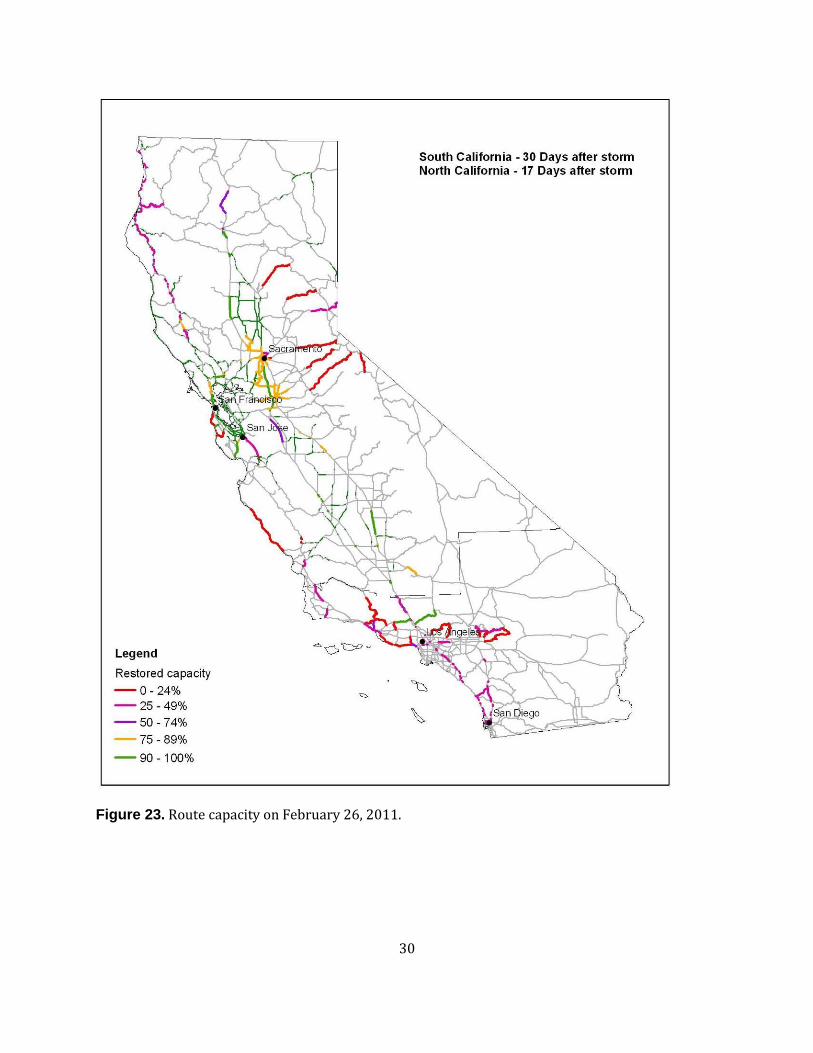
30

Figure 23. Route capacity on February 26, 2011.

31

Figure 24. Route capacity on April 27, 2011.

32

Figure 25. Route capacity on July 27, 2011.

33

Figure 26. Route capacity on January 27, 2012.

LIFELINE INTERACTION INVOLVING HIGHWAYS

Several panels noted how restoring their facilities depend on access. A large water district noted that it has critical pipelines that run through steep terrain, vulnerable to landslide, and that access to some of these lines is limited. Highway and roadway damage from landslides and bridge

34

damage could hinder repairs. Wastewater treatment near Long Beach likewise is affected by access, primarily by flooding: rising water might force employees at Terminal Island to abandon the treatment plant for their own safety. Furthermore, the southern California panel discussing water and wastewater noted that a number of water-supply pipelines are carried on highway or roadway bridges, some of which are subject to scour and hydrodynamic pressure.

Water-supply and wastewater treatment panels noted that they rely on supplies of chemicals that are carried on railway and trucks every few days. In the Sacramento panels, for example, it was observed that most of the chemicals used by water and wastewater treatment facilities are carried over I-80, which would be temporarily cut off.

LIMITATIONS OF HIGHWAY RESTORATION TIMELINE

Three important limitations of this scenario were recognized during the initial panel discussions. First, these restoration times may underestimate competition for limited resources. Second, these restoration timelines were laid out without full consideration of the needs for evacuation. Third, the landslide assessment for northern California was not available at the time of the panel discussions. New landslide information might affect the assessment of both damage and restoration. Other considerations that were overlooked during the panel discussions also may affect restoration.

OPPORTUNITIES TO ENHANCE HIGHWAY RESILIENCY

In discussions with highway panelists, the following possibilities were raised as opportunities to prevent highway damage or to recover faster:

Caltrans could purchase and stockpile Bailey bridges. Bailey bridges are portable, pre-fabricated trusses, primarily used by military engineering units to bridge up to 60-meter gaps (200 feet). These bridges do not require heavy equipment for construction; can be brought to the jobsite in trucks; and are strong enough for heavy traffic. Caltrans owns a few, probably not enough for the need suggested by ARkStorm. One panelist suggested that railroad flatcars might serve a similar purpose.

Preplan detours to enhance redundancy more quickly.

Prepare to move Caltrans equipment away from vulnerable areas in response to forecasts of severe weather.

Engage the contractor community to prepare for severe storms, for example, beginning with conversations with the Association of General Contractors in preparation for Golden Guardian 2011.

Have contracts in place for rental and repair of pumps, especially large pumps.

Consider dense string of webcams or CCTV cameras covering the roadway network for real-time virtual inspections.

Install strain gages and pore-water-pressure gages or other monitoring of known, deep-seated landslides.

Construct a system for 2-way 511 information with the public. USGS is in early conceptual planning of such an application called Did You See It? The application or Caltrans would require heavy filtering to keep the labor requirements for such a system affordable.

Plan for emergency housing of Caltrans workers and possibly their families.

Engage FEMA to allow post-disaster repair to higher standards than original construction.

Enhance evacuation procedures—consider benefits of earlier evacuations and of identifying evacuation centers based on weather reports.

35

Characterize and communicate uncertainty for better decisions by using weather and climate forecasts.

Enhance education and outreach—encourage people to have a family evacuation plan.

Coordinate with construction contractors to pre-position repair equipment.

Address growing labor limitations, for example, by partnering with cities, cross-training labor force for repairs, and identifying potential sources of repair crews. (One panelist mentioned crews from San Quentin State Prison)

Power

POWER FACILITIES AND SOURCES OF DAMAGE

The following power scenario is based on panel discussions with Southern California Edison, Los Angeles Department of Water and Power, the Sacramento Municipal Utility District, and California Utilities Emergency Association. In addition to these discussions, one of these entities, provided a detailed but confidential write-up following its internal considerations of the meteorology, flooding, windspeed, and landslide information provided to the panel. These materials are supplemented by data provided by utilities in follow-up conversations, and with data available in the Homeland Security Infrastructure Program (HSIP) Gold 2007 database, including the locations of essential facilities such as substations, power transmission routes, and wastewater treatment plants.

Note that representatives from Pacific Gas and Electric (PG&E) stated that they were unable to contribute at that time and that they would inform us later whether they would be able to participate; as of this writing they have not done so. The following, therefore, does not reflect the opinions or judgment of PG&E personnel. It does reflect our initial interpretation of the statements made during the other meetings, subsequent conversations with representatives of all the other lifeline service providers, and a fairly exhaustive review of newspaper accounts of 1986 and 1997 storm impacts on PG&E facilities, found in the Los Angeles Times, Sacramento Bee, and San Francisco Chronicle.

Several other power utilities were unable to attend panel meetings or were otherwise unable to estimate scenario damage and restoration. To estimate power outage and restoration for these remaining service areas, we make several assumptions, based on the panel discussions and other evidence cited below.

Sources of wind damage. According to panel participants, wooden crossbars and pole-mount transformers on distribution-voltage utility poles can be damaged by wind speeds as low as 60 miles per hour (mph). Moderate winds also can cause lines to sway, touch, and cause cross-phase shorting. Another common cause of wind damage is moderate wind speeds with windborne debris such as palm fronds blown onto lines causing shorts. Where winds are stronger, damage is more severe. Hurricane-force winds (75 mph and higher) can cause transmission lines to sway and cause cross-phase shorting, or cause electrical transmission towers or poles to collapse.

The panels did not postulate damage in high-wind regions (75 mph and higher). In Alpine, Inyo, Mono, and parts of El Dorado, Placer, Riverside, San Bernardino, and Tulare Counties, winds reach 75 to 125 mph. Figure 27 shows where high winds could threaten transmission lines. Note especially how high winds on the eastern side of the Sierra Nevada range coincide with the location of transmission lines.

36

Some documentation is available regarding power outage and restoration in south Florida in Hurricane Andrew (Porter and others, 1996). Peak gust velocities in a few Florida locations reached 170 mph, but in many places between Miami and Homestead peak gusts were in the range 100 mph to 125 mph (http://www.nhc.noaa.gov/prelims/1992andfig5.gif), similar to the most strongly affected regions in ARkStorm. About 55 percent of Florida Power and Light transmission lines were out of service because of Hurricane Andrew, (including 80 percent of the 230 kilovolt system and 60 percent of the 138 kilovolt system), along with about 70 percent of the distribution circuit miles. It took approximately 5 days for Florida Power and Light to restore service to 90 percent of its customers, and 30 days to reach 99 percent. Note that electrical facilities in hurricane country may be built to different standards in consideration of higher wind loads.

Figure 27. ARkStorm winds. Yellow indicates maximum windspeed in excess of 70 miles per hour. Red lines indicate electrical transmission lines.

http://www.nhc.noaa.gov/prelims/1992andfig5.gif�

37

Damage to wooden crossbars and pole-mount transformers was one of the more significant causes of system interruption. One panel estimated that 0.2 percent of customers in areas with peak gust velocities generally in the range of 45 to 75 mph could lose power because of wind damage to distribution poles. (Customers, as used here, are counted in electric-service meters, not inhabitants of residences or office buildings. A single-family dwelling, for example, would typically count as one customer.) Damage to poles in moderate windspeed areas is restored within 7 days of the storm.

We assume that 75 percent of customers in counties with higher winds - in the range of 75 to 125 mph - lose service, and that repairs would take 7 days to restore to 90 percent of customers and 4 weeks to restore power to almost all customers. This restoration curve, shown mathematically in Equation (1), is comparable to the restoration estimated in the confidential utility study for areas with similar, strong winds. The restoration curve is of the form:

01 expf t C r t (1)

where

f(t) is the fraction of customers with power at time t,

C0 is the initial fraction of customers without power (for example, 0.75),

t is time in days after the peak of the storm (January 27, 2011, in southern California, February 9, 2011, in northern California), and

r is a constant reflecting speed of restoration: 0.05 for very slow restoration and 0.30 for fast restoration. A value of 0.25 is used here.

Sources of flooding damage. Power plants, high-voltage substations (also called bulk substations) and control facilities can be sensitive to flooding damage in at least two important ways. Flooding can damage control equipment. High-voltage substations and generating plants have high-voltage transformers (50 to 200 megawatts (MW) at high-voltage substations and 300 to 500 MW at generating plants) that also can be damaged by flooding, for example, by flood-borne debris impacting the transformer and ancillary equipment. A problem is that these transformers are custom made, designed to match impedance at the facility it serves, and each location serves fairly large populations: a high-voltage substation for example can serve in excess of 200,000 people. The transformers are not interchangeable and are too expensive to stockpile backups beyond those available for normal operational redundancy. If one of these large transformers were damaged, it could take 6 months or more to replace. There is typically some redundancy, enough so that at any given high-voltage substation, for example, one of these transformers can be inoperative and the substation can still operate. In addition, agreements between utilities allow for the loan or sale of surplus or idle equipment in an emergency situation. However, flooding is a common-cause failure mode, the implication being that a flood can damage several components simultaneously, potentially damaging two or more of these transformers. Were this to happen, the utility would have to reroute power around the inoperative substation, which could take a few days, and immediately attempt to repair or replace the transformer once dewatering is completed. The reliability of the temporary grid layout would be reduced, meaning greater likelihood of power outages in the affected area.

Flooding also can damage equipment at generation facilities. If demand were high (less likely in the winter months in which the ARkStorm is postulated to occur), temporary emergency generation such as diesel generators—and the necessary fuel supplies—might have to be brought in to serve the affected areas. Figure 28 shows where power plants are located in relation to

38

flooded areas in four metropolitan areas of the state. While most power plants are located out of the flooded areas, some are inside, especially in Santa Clara County and Los Angeles.

(a) (b)

(c) (d)

Figure 28. Power plants (green diamonds) overlain with flooding (blue areas) in (a) San Francisco Bay Area, (b) Sacramento and Stockton, (c) Los Angeles and Orange Counties, and (d) San Diego.

POWER DAMAGE AND RESTORATION SCENARIO

One panel concluded that power is shut off to all flooded areas, and that electric-power utilities will restore power to customers who are affected by flooding shortly after the buildings are determined by local authorities to be safe to enter and occupy. We assume that this adds between 1 and 14 days to the downtime of all facilities with nonzero flood-related downtime. A median value

39

of 7 days is used throughout. However, since according to the HAZUS-MH flood module the time required to restore flooded buildings to operation is measured in months rather than days, restoration of power to flooded buildings is judged not to add significantly to their downtime.

However, it seems likely that there will be large areas that are not flooded, but that flooding of at least a few feet above grade (perhaps 3 or 4 feet) could damage the electrical and electronic equipment in the substations that serve the main stations. Of special concern are the high-voltage substations, discussed above, which tend to serve a large geographic area (on the order of 200,000 people). This damage could isolate those neighborhoods, either because the neighborhoods are near the end of a transmission or distribution line and lack a redundant path, or because all transmission to that area seems to run through substations that are flooded.

Using the HSIP Gold geospatial database of transmission lines and substations, we created an approximate inventory of the affected substations, and roughly approximated the fraction of the population of each county affected by the damage. We assumed that this fraction is without power, and that restoration takes up to 4 weeks, and applied the following restoration curve:

0

0

1

1 exp

f t C t d

C r t d t d (2)

where

C0 is the fraction of services assumed to be affected by substation flooding,

t is the number of days after the end of the storm (January 27 and February 9, in southern and northern California, respectively), and

d is the duration of flooding.

The foregoing considerations lead to the power restoration curves shown in table 1. The first column contains the county name, the second is Federal Information Processing Standard (FIPS) code. The column labeled peril denotes whether wind (W) or flood (F) dominates the cause of power failure to customers able to receive power. Column 4, labeled C0, denotes the estimated percentage of customers initially without power after the storm. The remaining columns reflect the estimated percentage of customers able to receive power that do have power service, by date. Figure 29 illustrates these curves in a few key locations.

It is estimated that the material and labor required to repair power facilities could cost between $300 million and $3 billion. For present purposes, the scenario posits the cost as the geometric mean (meaning the square root of the product) of these two figures, that is, $1 billion.

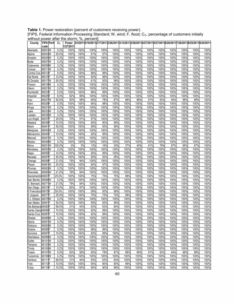
40

Table 1. Power restoration (percent of customers receiving power). [FIPS, Federal Information Processing Standard; W, wind; F, flood; C0

County

, percentage of customers initially without power after the storm; %, percent]

FIPS code

Peril C Power 0 1/27/2011

2/3/2011 2/10/2011 2/17/2011 2/26/2011 3/13/2011 3/28/2011 4/27/2011 5/27/2011 6/26/2011 7/26/2011 8/25/2011 9/24/2011

Alameda 06001 W 0.2% 100% 100% 100% 100% 100% 100% 100% 100% 100% 100% 100% 100% 100% Alpine 06003 W 25.0% 100% 100% 81% 97% 100% 100% 100% 100% 100% 100% 100% 100% 100% Amador 06005 W 0.2% 100% 100% 100% 100% 100% 100% 100% 100% 100% 100% 100% 100% 100% Butte 06007 W 0.2% 100% 100% 100% 100% 100% 100% 100% 100% 100% 100% 100% 100% 100% Calaveras 06009 W 0.2% 100% 100% 100% 100% 100% 100% 100% 100% 100% 100% 100% 100% 100% Colusa 06011 W 0.2% 100% 100% 100% 100% 100% 100% 100% 100% 100% 100% 100% 100% 100% Contra Cos 06013 F 5.0% 100% 100% 96% 99% 100% 100% 100% 100% 100% 100% 100% 100% 100% Del Norte 06015 F 10.0% 100% 100% 92% 99% 100% 100% 100% 100% 100% 100% 100% 100% 100% El Dorado 06017 W 50.0% 100% 100% 61% 93% 99% 100% 100% 100% 100% 100% 100% 100% 100% Fresno 06019 W 0.2% 100% 100% 100% 100% 100% 100% 100% 100% 100% 100% 100% 100% 100% Glenn 06021 W 0.2% 100% 100% 100% 100% 100% 100% 100% 100% 100% 100% 100% 100% 100% Humboldt 06023 F 5.0% 100% 100% 96% 99% 100% 100% 100% 100% 100% 100% 100% 100% 100% Imperial 06025 F 8.0% 92% 99% 100% 100% 100% 100% 100% 100% 100% 100% 100% 100% 100% Inyo 06027 W 50.0% 50% 58% 60% 78% 87% 88% 89% 91% 93% 94% 96% 98% 100% Kern 06029 F 5.0% 100% 100% 95% 98% 100% 100% 100% 100% 100% 100% 100% 100% 100% Kings 06031 W 0.2% 100% 100% 100% 100% 100% 100% 100% 100% 100% 100% 100% 100% 100% Lake 06033 W 0.2% 100% 100% 100% 100% 100% 100% 100% 100% 100% 100% 100% 100% 100% Lassen 06035 W 0.2% 100% 100% 100% 100% 100% 100% 100% 100% 100% 100% 100% 100% 100% Los Angel. 06037 F 30.0% 70% 91% 97% 100% 100% 100% 100% 100% 100% 100% 100% 100% 100% Madera 06039 F 10.0% 100% 100% 90% 90% 99% 100% 100% 100% 100% 100% 100% 100% 100% Marin 06041 F 50.0% 100% 100% 59% 93% 99% 100% 100% 100% 100% 100% 100% 100% 100% Mariposa 06043 W 0.2% 100% 100% 100% 100% 100% 100% 100% 100% 100% 100% 100% 100% 100% Mendocino 06045 F 10.0% 100% 100% 92% 99% 100% 100% 100% 100% 100% 100% 100% 100% 100% Merced 06047 W 0.2% 100% 100% 100% 100% 100% 100% 100% 100% 100% 100% 100% 100% 100% Modoc 06049 W 0.2% 100% 100% 100% 100% 100% 100% 100% 100% 100% 100% 100% 100% 100% Mono 06051 W 100.0% 0% 5% 13% 16% 30% 37% 45% 61% 79% 87% 95% 97% 100% Monterey 06053 W 0.2% 100% 100% 100% 100% 100% 100% 100% 100% 100% 100% 100% 100% 100% Napa 06055 F 10.0% 100% 100% 92% 99% 100% 100% 100% 100% 100% 100% 100% 100% 100% Nevada 06057 F 50.0% 100% 100% 50% 50% 95% 100% 100% 100% 100% 100% 100% 100% 100% Orange 06059 F 21.0% 79% 94% 100% 100% 100% 100% 100% 100% 100% 100% 100% 100% 100% Placer 06061 W 20.0% 100% 100% 84% 97% 100% 100% 100% 100% 100% 100% 100% 100% 100% Plumas 06063 W 0.2% 100% 100% 100% 100% 100% 100% 100% 100% 100% 100% 100% 100% 100% Riverside 06065 W 21.0% 79% 94% 100% 100% 100% 100% 100% 100% 100% 100% 100% 100% 100% Sacramento 06067 F 25.0% 100% 100% 75% 75% 75% 98% 100% 100% 100% 100% 100% 100% 100% San Benito 06069 W 0.2% 100% 100% 100% 100% 100% 100% 100% 100% 100% 100% 100% 100% 100% S. Bernard. 06071 W 21.0% 79% 94% 100% 100% 100% 100% 100% 100% 100% 100% 100% 100% 100% San Diego 06073 F 15.0% 85% 97% 100% 100% 100% 100% 100% 100% 100% 100% 100% 100% 100% S Francisco 06075 F 50.0% 100% 100% 59% 93% 99% 100% 100% 100% 100% 100% 100% 100% 100% S Joaquin 06077 F 25.0% 100% 100% 75% 75% 75% 98% 100% 100% 100% 100% 100% 100% 100% S L Obispo 06079 W 0.2% 100% 100% 100% 100% 100% 100% 100% 100% 100% 100% 100% 100% 100% San Mateo 06081 F 50.0% 100% 100% 59% 93% 99% 100% 100% 100% 100% 100% 100% 100% 100% Sta Barbara 06083 F 69.0% 31% 44% 63% 63% 84% 100% 100% 100% 100% 100% 100% 100% 100% Santa Clara 06085 F 10.0% 100% 100% 92% 99% 100% 100% 100% 100% 100% 100% 100% 100% 100% Santa Cruz 06087 F 10.0% 100% 100% 92% 99% 100% 100% 100% 100% 100% 100% 100% 100% 100% Shasta 06089 W 0.2% 100% 100% 100% 100% 100% 100% 100% 100% 100% 100% 100% 100% 100% Sierra 06091 W 0.2% 100% 100% 100% 100% 100% 100% 100% 100% 100% 100% 100% 100% 100% Siskiyou 06093 W 0.2% 100% 100% 100% 100% 100% 100% 100% 100% 100% 100% 100% 100% 100% Solano 06095 F 5.0% 100% 100% 96% 99% 100% 100% 100% 100% 100% 100% 100% 100% 100% Sonoma 06097 F 10.0% 100% 100% 92% 99% 100% 100% 100% 100% 100% 100% 100% 100% 100% Stanislaus 06099 W 0.2% 100% 100% 100% 100% 100% 100% 100% 100% 100% 100% 100% 100% 100% Sutter 06101 W 0.2% 100% 100% 100% 100% 100% 100% 100% 100% 100% 100% 100% 100% 100% Tehama 06103 W 0.2% 100% 100% 100% 100% 100% 100% 100% 100% 100% 100% 100% 100% 100% Trinity 06105 W 0.2% 100% 100% 100% 100% 100% 100% 100% 100% 100% 100% 100% 100% 100% Tulare 06107 W 5.0% 50% 58% 60% 78% 87% 88% 89% 91% 93% 94% 96% 98% 100% Tuolumne 06109 W 0.2% 100% 100% 100% 100% 100% 100% 100% 100% 100% 100% 100% 100% 100% Ventura 06111 F 69.0% 31% 44% 63% 63% 84% 100% 100% 100% 100% 100% 100% 100% 100% Yolo 06113 F 10.0% 100% 100% 90% 90% 90% 99% 100% 100% 100% 100% 100% 100% 100% Yuba 06115 F 10.0% 100% 100% 90% 90% 99% 100% 100% 100% 100% 100% 100% 100% 100%

41

Figure 29. Power restoration curves at a few key locations, showing percentage of customers capable of receiving power at selected times.

LIFELINE INTERACTION INVOLVING POWER

As with ShakeOut, damage to other lifelines can impact the restoration of power. As examples, roadway damage can hinder electric utilities from getting to affected areas and performing repairs. Telecommunications failure can hinder the reporting of any damage to the utilities, as well as hindering repair coordination.

OPPORTUNITIES TO ENHANCE POWER RESILIENCY

One panelist observed that all California electric utilities are required to perform preventive maintenance under California Public Utilities Commission (CPUC) general order 165. He also noted that all California electric utilities are familiar with FEMA reporting and the appropriate forms for financial relief. The following methods for enhancing power resiliency were identified during panel discussions or in subsequent conversations and correspondence.

Convert overhead bare conductors to underground cable in conduit. However, this conversion can be very costly (up to $1 million per mile in urban areas, or 5 times the cost of new overhead construction). This conversion raises new issues and challenges such as coordinating and routing several congested utilities, providing an adequate cathodic protection and protection from water. Lifecycle costs might be different and would have to be investigated to determine if the economical feasibility to perform this conversion.

Elevate transformers and control equipment at substations to protect from flooding.

Pre-position repair crews based on severe weather forecasts.

0%

25%

50%

75%

100%

1/27/2011 3/28/2011 5/27/2011 7/26/2011 9/24/2011 11/23/2011

Pow

er s

ervi

ce (

% o

f cus

tom

ers

capa

ble

of r

ecei

ving

pow

er)

Los Angeles

San Francisco

Sacramento

San Diego

Mono

(High winds)

(Lower winds)

42

Send utility inspection crews to check for hazardous conditions at substations.

Train utility workers to document damage in the detail required for government assistance.

Promote the design and acquisition of a mobile, high-voltage transformer that has ability for the user to easily change the internal impedance and the turns ratio. This innovation would mitigate the problem of long lead times to replace damaged high-voltage transformers. One panelist acknowledged the potential value of such a transformer; another expressed skepticism that such a design is, in fact, feasible.

One panelist suggested promoting the design and acquisition of a mobile, modular substation complete with all the relays, circuit breakers, and controls capable to service one distribution station or a receiving station.

Finally, there seemed to be broad consensus that mutual assistance among power utilities is key in any major disaster. Having the right spare equipment also is imperative.

LIMITATIONS OF ESTIMATES WITH RESPECT TO POWER

This approach was a best estimate for a highly uncertain situation. It is particularly uncertain for the areas not addressed by panel discussions. Damage to power system components from landslides is not accounted for, nor is any special consideration made of shutdown of nuclear power plants or of other generating facilities not in the flooded areas. PG&E and some other utilities were unable to participate in developing the scenario. Had these utilities participated, the scenario would have been more accurate. These limitations argue for a more thorough assessment by PG&E and other utilities.

Wastewater Treatment

WASTEWATER FACILITIES AND SOURCES OF DAMAGE

Wastewater treatment systems typically comprise sewer pipes (laterals from customers to the street; collectors, truck sewers, interceptors, and outflow structures), pumping stations (also called lift stations), and wastewater treatment plants (WWTPs). Pipes tend to be relatively brittle, constructed of vitrified clay or reinforced concrete, but some structures are aging, brick-lined tunnels or tunnels lined with unreinforced concrete. Sewer flow is typically driven by gravity and aided by lift stations. Sewer pipes can be damaged by landsliding and in some cases by scour, especially external scour to shallow cut-and-cover tunnels. Sewer pipes also can be damaged by ground settlement and other movement aggravated by soil becoming saturated after multiple storms. The primary cause of damage to pumping stations and WWTPs discussed in panels was flooding damage to electrical equipment and sediment getting into pumps. We begin by discussing damage to WWTPs.

Although there is an incomplete spatial database of WWTPs, discussed below, we are unaware of any complete inventory or GIS system describing all or even a significant fraction of California sewer systems. Roughly 135 WWTPs and an unknown number of sewage pumping stations (also called lift stations) operate in California. Flooding can damage these facilities, especially by damaging electrical equipment or by floating or buckling storage tanks. The degree of damage to electrical equipment depends on whether the equipment is deenergized before flooding. The damage is worse if the equipment is not deenergized before being powered down, which can happen if flooding occurs without sufficient advanced warning or at night when minimal crews are on hand to shut down equipment. When a WWTP or lift station is flooded and shut down, untreated sewage may emerge from nearby maintenance holes and wetwells, and flow by gravity overland to

43

nearby rivers or shorelines, contaminating a radius of up to ½ to 1 mile around the point of sewage discharge if the flooding reaches that far. Once the sewage enters a stream, creek, or river, the distance of contamination can far exceed the ½ to 1 mile distance. The contaminated area potentially can require evacuation of homes and businesses. In addition to the soft-term health impacts, any agricultural fields with sewerage in nearby streams may cause the crops to be deemed unsafe.

WWTPs tend to be in low-lying areas and, therefore, more subject to flooding than the population served. A spatial database of WWTPs is available in the HSIP Gold 2007 database. It shows 21 WWTPs in inundated areas (out of 113 California WWTPs shown in database). The HSIP Gold 2007 database appears to be incomplete, however, and is missing at least 24 WWTPs, 7 of which lie in the hypothetically flooded areas: 2 in Amador County (neither flooded), 1 in Colusa County (not flooded), 4 in Imperial County (none flooded), 3 in Madera County (none flooded), 1 in Modoc County (not flooded), 1 in Los Angeles County (flooded), 1 in Sacramento County (not flooded, because of floodwall protection designed for 500-year flooding), 2 in San Francisco (neither in the hypothetically flooded areas, however), 3 in Santa Cruz (none flooded), 1 in Sutter County (flooded), 3 in Tehama County (1 possibly flooded), 3 in Yolo County (all in the hypothetically flooded areas). The list of counties with known WWTPs in the scenario flooded area is shown in table 2. The table lists, by county, the peak flooding depth (anywhere in the county) along with flooding duration, number of WWTPS known to be in the hypothetically inundated area, both as a number and as a fraction of the WWTPs shown in the HSIP Gold 2007 database and supplemented here by Google Earth searches. (After the development of the table, we found that an U.S. Environmental Protection Agency database reflected much of the missing information, though not all, and not in a convenient format. The database would have required extensive interpretation to be useful, and so is not reflected here.) Table 2. Wastewater treatment plants (WWTP) in scenario flooding areas, per county. With maximum flooding, duration of flooding, number and percentage of flooded WWTPs. [ft, feet; WWTPs, wastewater treatment plants; %, percent; <, less than]

County Peak depth, ft Duration, days Flooded WWTPs % Total WWTPs Alameda 3-10 <0.5 1 25 Butte <3 0.5-3 1 100 Contra Costa 3-10 <0.5 1 10 Los Angeles 3-10 <0.5 2 20 Marin 3-10 <0.5 2 40 Orange 3-10 <0.5 4 57 Tehama <3 0.5-3 1 33 San Diego 3-10 <0.5 1 17 San Joaquin 10-20 14-28 2 67 San Mateo 3-10 <0.5 2 67 Santa Clara 3-10 <0.5 3 100 Sonoma 3-10 <0.5 1 100 Sutter 3-10 3-14 1 100 Ventura 3-10 <0.5 1 25 Yolo 10-20 14-28 3 100 Yuba 3-10 3-14 1 100 Total 27

44

WASTEWATER DAMAGE AND RESTORATION SCENARIO

Following is a description of damage and restoration discussed in the Pasadena wastewater treatment panel. This description is offered as a pattern for emergency planning purposes.

Flooding at pumping stations and WWTPs. In Los Angeles, the scenario imagines that the Donald C. Tillman and Terminal Island WWTPs are flooded. The former floods the central and western San Fernando Valley. Raw sewage emerges from the 50 nearest maintenance holes, and flows overland to the Los Angeles River, causing a hazardous material condition that could trigger evacuation of homes and businesses that were not otherwise flooded, and shutting down roads through the affected area.

At Terminal Island, the Terminal Way pumping plant is submerged, and sewage is not pumped to Terminal Island because of the loss of power. Terminal Island is in danger of being isolated, causing a life-safety threat to employees, and is evacuated. Raw sewage emerges near the Terminal Way pumping plant and runs untreated to the Pacific Ocean. Near Venice Beach, the Venice Pumping Plant is briefly submerged, and sewage is not pumped to the Hyperion WWTP. Instead the sewage emerges from wetwells and maintenance holes between Santa Monica and Venice and runs overland to the Pacific Ocean. Similar effects would occur near other flooded WWTPs.

Pipeline damage and restoration. Landslides cause localized damage to sewer pipes throughout the area. Flooding also can carry large amounts of sediment into sewer pipes; one panel estimated that 10-15 percent of pipes in flooded area will have large amounts of sediment that will need to be cleaned out. Sewer pipe damage will continue to emerge for several months after the storm; the Menlo Park panel estimated that repairs to sewer pipes in the San Francisco Bay area could cost on the order of $60 million, realized over the 6 months after the storm. Scaling up solely by population, this suggests statewide sewer pipe repairs costing on the order of $300 million, that is, roughly $9 per resident, on average. Cities with more intense rainfall and older sewer systems will experience greater-than-average sewer damage rates.

In Los Angeles, one important point of significant damage is the north outfall sewer, which zigzags under the Los Angeles River. This aging structure is partly brick-lined, partly lined with unreinforced concrete. It is a shallow, cut-and-cover structure, and it seemed possible to some panelists that the sewer could be damaged by external scour near the river.

It is uncertain how long repairs would take to restore damaged electrical equipment. One panel felt that, if the equipment is deenergized before being wetted, the equipment can be dried and reenergized within a day of floodwaters receding; otherwise short-circuited equipment might take weeks or more to replace. Another panel disagreed with the notion that deenergized equipment could be dried and quickly restored to service, and felt instead that flooded electrical equipment could be contaminated with silt and have to be replaced, which might take months (one panel suggested 3-6 months). As a middle ground, we have perhaps optimistically assumed that service is restored within 4 weeks after floodwaters recede from WWTPs. This assumption needs checking.

For purposes of estimating economic impacts of the failure of sewer service, the percentage shown in table 2 is taken as the fraction of customers whose sewer service is rendered unavailable beginning near the peak of the storm, then continuing for the duration of flooding noted in the table, with an additional 2 days to 4 weeks, to account for the time required to repair or replace electrical equipment. Service restoration is assumed to follow the same exponential curve form as

45

before, that is, Equation (2), where now f(t) denotes the fraction of customers with sewer service, C0 denotes the fraction of services assumed to be affected by WWTP flooding, t again is the number of days after the end of the storm (January 27 and February 9, in southern and northern California, respectively), and d is the flooding duration. The parameter r is a constant, this time set to 0.15 to cause the calculated fraction of sewer services restored to be 65 percent of services within 1 week after flooding recedes, and 99 percent restored within 4 weeks after flooding recedes.

The results are tabulated in table 3. Note well that C0 includes all customers, including residences, businesses, and other facilities that are rendered unoccupiable by flooding or other damage.

46

Table 3. Sewer service restoration per county over time after the ARkStorm. [FIPS, Federal Information Processing Standard; C0County

, percentage of customers initially without power after the storm; %, percent] FIPS C 1/27/11 0 2/3/11 2/10/11 2/17/11 2/26/11 3/13/11 3/28/11 4/27/11 5/27/11 6/26/11 7/26/11 8/25/11 9/24/11

Alameda 06001 25% 100% 100% 78% 92% 98% 100% 100% 100% 100% 100% 100% 100% 100% Alpine 06003 0% 100% 100% 100% 100% 100% 100% 100% 100% 100% 100% 100% 100% 100% Amador 06005 0% 100% 100% 100% 100% 100% 100% 100% 100% 100% 100% 100% 100% 100% Butte 06007 100% 100% 100% 0% 59% 89% 99% 100% 100% 100% 100% 100% 100% 100% Calaveras 06009 0% 100% 100% 100% 100% 100% 100% 100% 100% 100% 100% 100% 100% 100% Colusa 06011 0% 100% 100% 100% 100% 100% 100% 100% 100% 100% 100% 100% 100% 100% Contra Costa 06013 10% 100% 100% 91% 97% 99% 100% 100% 100% 100% 100% 100% 100% 100% Del Norte 06015 0% 100% 100% 100% 100% 100% 100% 100% 100% 100% 100% 100% 100% 100% El Dorado 06017 0% 100% 100% 100% 100% 100% 100% 100% 100% 100% 100% 100% 100% 100% Fresno 06019 0% 100% 100% 100% 100% 100% 100% 100% 100% 100% 100% 100% 100% 100% Glenn 06021 0% 100% 100% 100% 100% 100% 100% 100% 100% 100% 100% 100% 100% 100% Humboldt 06023 0% 100% 100% 100% 100% 100% 100% 100% 100% 100% 100% 100% 100% 100% Imperial 06025 0% 100% 100% 100% 100% 100% 100% 100% 100% 100% 100% 100% 100% 100% Inyo 06027 0% 100% 100% 100% 100% 100% 100% 100% 100% 100% 100% 100% 100% 100% Kern 06029 0% 100% 100% 100% 100% 100% 100% 100% 100% 100% 100% 100% 100% 100% Kings 06031 0% 100% 100% 100% 100% 100% 100% 100% 100% 100% 100% 100% 100% 100% Lake 06033 0% 100% 100% 100% 100% 100% 100% 100% 100% 100% 100% 100% 100% 100% Lassen 06035 0% 100% 100% 100% 100% 100% 100% 100% 100% 100% 100% 100% 100% 100% Los Angeles 06037 20% 80% 93% 97% 99% 100% 100% 100% 100% 100% 100% 100% 100% 100% Madera 06039 0% 100% 100% 100% 100% 100% 100% 100% 100% 100% 100% 100% 100% 100% Marin 06041 40% 100% 100% 64% 87% 97% 100% 100% 100% 100% 100% 100% 100% 100% Mariposa 06043 0% 100% 100% 100% 100% 100% 100% 100% 100% 100% 100% 100% 100% 100% Mendocino 06045 0% 100% 100% 100% 100% 100% 100% 100% 100% 100% 100% 100% 100% 100% Merced 06047 0% 100% 100% 100% 100% 100% 100% 100% 100% 100% 100% 100% 100% 100% Modoc 06049 0% 100% 100% 100% 100% 100% 100% 100% 100% 100% 100% 100% 100% 100% Mono 06051 0% 100% 100% 100% 100% 100% 100% 100% 100% 100% 100% 100% 100% 100% Monterey 06053 0% 100% 100% 100% 100% 100% 100% 100% 100% 100% 100% 100% 100% 100% Napa 06055 0% 100% 100% 100% 100% 100% 100% 100% 100% 100% 100% 100% 100% 100% Nevada 06057 0% 100% 100% 100% 100% 100% 100% 100% 100% 100% 100% 100% 100% 100% Orange 06059 57% 43% 79% 93% 97% 99% 100% 100% 100% 100% 100% 100% 100% 100% Placer 06061 0% 100% 100% 100% 100% 100% 100% 100% 100% 100% 100% 100% 100% 100% Plumas 06063 0% 100% 100% 100% 100% 100% 100% 100% 100% 100% 100% 100% 100% 100% Riverside 06065 0% 100% 100% 100% 100% 100% 100% 100% 100% 100% 100% 100% 100% 100% Sacramento 06067 0% 100% 100% 100% 100% 100% 100% 100% 100% 100% 100% 100% 100% 100% San Benito 06069 0% 100% 100% 100% 100% 100% 100% 100% 100% 100% 100% 100% 100% 100% San Bernardino 06071 0% 100% 100% 100% 100% 100% 100% 100% 100% 100% 100% 100% 100% 100% San Diego 06073 17% 83% 94% 98% 99% 100% 100% 100% 100% 100% 100% 100% 100% 100% San Francisco 06075 0% 100% 100% 100% 100% 100% 100% 100% 100% 100% 100% 100% 100% 100% San Joaquin 06077 67% 100% 100% 33% 33% 33% 87% 99% 100% 100% 100% 100% 100% 100% San Luis Obispo 06079 0% 100% 100% 100% 100% 100% 100% 100% 100% 100% 100% 100% 100% 100% San Mateo 06081 50% 100% 100% 55% 84% 96% 100% 100% 100% 100% 100% 100% 100% 100% Santa Barbara 06083 0% 100% 100% 100% 100% 100% 100% 100% 100% 100% 100% 100% 100% 100% Santa Clara 06085 100% 100% 100% 11% 69% 92% 99% 100% 100% 100% 100% 100% 100% 100% Santa Cruz 06087 0% 100% 100% 100% 100% 100% 100% 100% 100% 100% 100% 100% 100% 100% Shasta 06089 0% 100% 100% 100% 100% 100% 100% 100% 100% 100% 100% 100% 100% 100% Sierra 06091 0% 100% 100% 100% 100% 100% 100% 100% 100% 100% 100% 100% 100% 100% Siskiyou 06093 0% 100% 100% 100% 100% 100% 100% 100% 100% 100% 100% 100% 100% 100% Solano 06095 0% 100% 100% 100% 100% 100% 100% 100% 100% 100% 100% 100% 100% 100% Sonoma 06097 100% 100% 100% 11% 69% 92% 99% 100% 100% 100% 100% 100% 100% 100% Stanislaus 06099 0% 100% 100% 100% 100% 100% 100% 100% 100% 100% 100% 100% 100% 100% Sutter 06101 100% 100% 100% 0% 0% 74% 97% 100% 100% 100% 100% 100% 100% 100% Tehama 06103 33% 100% 100% 67% 86% 96% 100% 100% 100% 100% 100% 100% 100% 100% Trinity 06105 0% 100% 100% 100% 100% 100% 100% 100% 100% 100% 100% 100% 100% 100% Tulare 06107 0% 100% 100% 100% 100% 100% 100% 100% 100% 100% 100% 100% 100% 100% Tuolumne 06109 0% 100% 100% 100% 100% 100% 100% 100% 100% 100% 100% 100% 100% 100% Ventura 06111 25% 75% 91% 97% 99% 100% 100% 100% 100% 100% 100% 100% 100% 100% Yolo 06113 100% 100% 100% 0% 0% 0% 81% 98% 100% 100% 100% 100% 100% 100% Yuba 06115 100% 100% 100% 0% 0% 74% 97% 100% 100% 100% 100% 100% 100% 100%

47

LIFELINE INTERACTION INVOLVING WASTEWATER TREATMENT

Some lift stations may be equipped with backup power, although none were identified in our panels. Lacking commercial power or backup power these stations cannot operate. Many WWTPs are provided with onsite electrical power. A San Francisco panelist reported that all San Francisco WWTPs have emergency generators (generally somewhat elevated above grade) with sufficient capacity to power the WWTP during normal power interruptions, and believed the same to be true at East Bay Municipal Utility District (EBMUD) facilities. If the emergency generators run on diesel or other fuel other than piped natural gas, then the generators are susceptible to running out of fuel within 3-5 days if roadway damage or flooding were to affect fuel delivery. We, therefore, assume that, in general, when commercial power is unavailable, lift stations do not operate but many WWTPs may function. Furthermore, since sewer lines are co-located with streets, where lift stations and WWTPs cease to function, untreated sewage can emerge onto streets, causing hazmat conditions that cause road closures and hinder repairs to other lifelines. One panel estimated that, in Marin County, 2 to 5 percent of street miles might have raw sewage on roads. Cleaning up sewage spills often uses large amounts of fresh water.

RESILIENCY AND RESEARCH NEEDS FOR WASTEWATER SERVICE

The following opportunities were discussed for enhancing the resilience of wastewater service, either by reducing damage, by speeding restoration, or by otherwise reducing the impacts of damage.

Utilities (perhaps in collaboration with FEMA) anticipate and budget for the opportunity to restore wastewater systems to greater-than-pre-storm capacity. Some panelists believed that when using FEMA public assistance funds after federally declared disasters, facilities had to be restored to predisaster condition, that is, that FEMA would not provide the equivalent amount of funding if the utility restored to higher capacity, even if the utility made up the difference in cost itself. A FEMA program officer involved in the discussion was unsure of the accuracy of that statement, but nonetheless the subject is worth investigating.

Consider adding or enhancing floodwalls around critical facilities such as WWTPs, or elevating sensitive electrical and mechanical equipment, conduit, and bus bar (a bar that conducts electrical current) above extreme flooding stage.

Enhance backup power and onsite fuel capabilities where cost effective. Where FEMA hazard mitigation grants are available, consider among the benefits the avoided health and agricultural impacts and loss of functionality of evacuated dwellings and businesses. Onsite backup power can produce benefits in terms of losses avoided from earthquake as well as floods.

Develop or review contingency plans for monitoring weather forecasts and the impacts on local facilities; and for deenergizing sensitive electrical equipment, especially considering night-shift crews, when there are fewer staff available; and facilities with limited ability to see rising rivers nearby.

Stockpile common electrical equipment or create a common national database of backup electrical equipment and the means to transfer and install it quickly.

One panelist (Craig Davis) recommended that “drains, conduits (storm channels and pipes), and storm detention/retention basins be inspected periodically (probably at least annually) and where needed, cleaned of debris and sediments to ensure they retain their design capacity. Drains or channels also include the benches placed on slopes to help protect the slope stability. This might sound like something that is obvious, which it is, but it costs money and time and many organizations and private property owners simply do not do this. We inspect and clean in some areas, but not all. Even where known, we cannot always find the labor or money to clean out some areas for every winter. In 2005, we learned that

48

the lack of even some of the simplest cleaning of bench drains on our slopes can be critical to preventing storm related slope stability and debris flow problems. Once a problem arises it is easy to see that the cost of repair is far greater than the annual saving by not keeping the drains, conduits, and basins cleaned on an annual basis…. Some agencies do a pretty good job with the basins and major channels. One that stands out in my mind is LA County Flood Control District.”

We encountered some limitations of available knowledge in preparing this scenario that suggest research needs:

The HSIP Gold 2007 database has major gaps in data on the location of wastewater treatment facilities (WWTPs). Furthermore, there appears to be no information linking WWTPs to particular watersheds, nor is there data about the locations of major sewer lines or lift stations. There is no centralized information about WWTP capacities, provision of onsite power, elevation of electrical and sensitive mechanical and plumbing equipment is available. WWTP facilities and vulnerabilities vary enormously, which makes the performance of studies such as this one problematic especially if the studies cross district boundaries.

There was a difference of opinion as to whether flooded electrical equipment needs to be replaced, and no information is readily available as to replacement times. (This latter point is changing with the development of ATC-58, a FEMA-funded effort to codify 2nd-generation performance-based earthquake engineering. Part of that effort involves compiling a database of repair and replacement time for common mechanical, electrical, and plumbing equipment.)

Water Supply

WATER FACILITIES AND SOURCES OF DAMAGE

About 95 percent of Californians get their water from a public, municipal source. About 324 water districts in California and more than 8,000 small public water systems serve 6 to 7 percent of the population. Figure 30 shows the larger districts, including federal, regional, state, and municipal water districts. A map of the state's major water projects is shown in figure 31. A map of about 1,500 dams in the state in the HSIP Gold 2007 database is shown in figure 32; these include the 1,250 dams regulated by the California Division of Safety of Dams (DSOD). The other 250 dams are either federal dams, or exempt, or below the size threshold that would place the dams under DSOD jurisdiction. Between 60 and 65 percent of statewide water use comes from surface-water supplies; the balance from ground water, though nearly half of Californians rely to some extent on ground water. Ground-water use is most intense in regions with limited access to surface water. According to the California Department of Water Resources, over 80 percent of water use in the Central Coast region comes from ground water, as does about 70 percent of water use in the southern Sierra. The general geographic distribution of the state's 35,000 monitored wells is shown in figure 33, which shows wells for which the California Department of Water Resources maintains hydrographic data in its Water Data Library (WDL) system. The drinking water for about 1.6 million people comes from over 600,000 private domestic wells (not shown).

WATER SUPPLY DAMAGE AND RESTORATION SCENARIO

During panel discussions with water-supply service providers, several significant damage modes were identified. One was contamination of wellheads and flood damage to electrical equipment serving pumps at the wellhead. The damage mode was identified by representatives of a southern California water district serving 65,000 people, who observed that the district had hundreds of wellheads in dry riverbeds, and that some might have poor sanitary seals. Within one basin, it seemed realistic that a limited plume of untreated sewage could contaminate a significant

49

part of the aquifer in one basin, interrupting water-supply service to perhaps 25 percent of the utility’s customers. Restoration would involve repairing damaged electrical equipment and cleaning the wells. Repairs to that system could cost $100 million and take 2 to 4 weeks if the system were properly shut down before electrical shorts could occur; otherwise repairs could plausibly cost $1 billion and take up to 6 months. Scaling up from the smaller figure for this relatively small water district, repair costs for water supply for a larger water district could plausibly range from $1-$10 billion; we have estimated $3 billion here.

Two northern California water utilities that rely on ground water echoed the same concern, suggesting that it was realistic for half of their wells to be impacted. Representatives from one of the two utilities felt that its wellheads could be disinfected and water supply restored approximately 3 days after floodwaters receded and power was restored. Its wellheads are supplied by backup power—emergency generators powered by natural gas with some onsite storage—although because the electrical equipment is located at ground level, the generator and its electrical equipment would be damaged, rendered nonfunctional, and have to be replaced.

Other damage modes identified during panel discussions include:

Flooding damage to electrical and other equipment at water treatment plants (WTP). Panelists' estimates for restoration time varied widely, from 2 days to 6 months, generally over the question of whether the flooded electrical equipment could be dried and reenergized, or would have to be replaced. One panelist suggested that WTP serving the entire city of Sacramento would be inoperative for up to 3-6 months.

Loss of water transmission from northern to southern California because of damage from overtopping of levees in the Sacramento Delta or aqueduct damage caused by flash flooding. (For example, flash flooding in the Arroyo Pasajaro could disable the California Aqueduct between Tracy and Coalinga, as happens elsewhere periodically.) About half of southern California’s water comes from the Delta. Panel participants felt that it was realistic for levee repairs necessary to restore conveyance to southern California to take 3 months. (Not the same as the amount of time required to repair all levee breaches and dewater flooded islands, which would probably be several years.) Note, however, that between ground water and other local supplies, alternate routes, reduced winter demand, and conservation, panelists felt that southern California would not lack for water solely because of levee and aqueduct damage to northern California supplies. Panelists and others have noted that southern California has one of the most robust water-supply systems in the world.

Greatly increased turbidity in surface water because of runoff carrying sediments into reservoirs and because of erosion of the banks of reservoirs. Panelists concluded that in southern California at least, water quality would be a far more significant problem than quantity, primarily in that filters would have to be flushed frequently, and that there would be concerns of contaminants from runoff potentially requiring extended boil-water orders.

Loss of power. Many water service providers rely on power to operate pumps. Those pumps that have onsite backup power tend to have generators and electrical equipment at grade, meaning that if they are flooded, the generator and electrical equipment would be damaged, rendered inoperative, and have to be replaced.

Landslides could damage tanks on hillsides. The example cited was tanks near the Seven Oaks Dam in Devils Canyon.

Pipes that cross canyons could be damaged by debris flows. The example cited was debris flow out of the Santa Ana River into the pickup for North Fork Irrigation and the City of Redlands. The pipe serves about 50,000 people, though it is not the sole source of water.

Pipes collocated on bridges could be damaged if the bridges are damaged, for example, by foundation scour.

50

Debris flows could damage local water distribution systems, for example, by breaking enough service connections where the pipes rise into houses to reduce pressure locally until the damage can be valved off. Panelists and ARkStorm landslide experts estimated that perhaps 100-200 neighborhoods of on the order of 20 to 50 homes each could lose water supply as a result of debris flows.

From these observations, producing a quantitative, statewide damage and restoration scenario for water supply is challenging. The damage and restoration scenario depicted here is, therefore, intended primarily for purposes of economic analysis, and relies on the following simplifications: Water supply impacts in Central Valley counties are primarily caused by flooding damage to electrical equipment at water treatment plants and wellheads, and contamination of wells. The Central Valley counties with the most severe flooding are Glenn, Butte, Colusa, Sutter, Yuba, Yolo, Sacramento, San Joaquin, Merced, and Kings; for these we assume that 50 percent of water supply is lost during the duration of flooding and for 14 days thereafter. Supply is then gradually restored, reaching 99 percent restoration within 3 months. The same restoration curve is applied to Orange County, because of severe flooding. In Central Valley counties with less flooding (Fresno, Madera and Kern), 15 percent of the county's water supply is assumed to be impacted during the duration of flooding plus 7 days, and is gradually restored, reaching 99 percent of pre-storm capacity within 30 days. In southland counties with moderate flooding (Los Angeles and Ventura), we assume that the primary impacts are contamination of wells and damage to electrical equipment at wellheads, affecting 10 percent of water supply for the duration of flooding plus 7 days, with 99 percent of capacity restored within 30 days. Loss of water supply in other counties is assumed to be negligible from a macroeconomic perspective. Results are shown in table 4 and figure 34.

51

Figure 30. The larger water districts among the 324 federal, regional, state, and municipal water districts in California. Colors of districts varied to improve visibility.

52

Figure 31. Major state water projects (modified from California Department of Water Resources, 2005).

Water Projects After 1998

Diamond Valley Lake

East Branch Extension

Crafton Hills Reservoir

Olivenhain Dam

53

Figure 32. Locations of California dams (yellow triangles). Only a fraction is for water-supply purposes.

54

Figure 33. Locations of 35,000 water wells in California (Department of Water Resources Integrated Water Resources Information System).

55

Table 4. Water service restoration per county over time. [FIPS, Federal Information Processing Standard; C0County

, percentage of customers initially without power after the storm; %, percent] FIPS C0 1/27/2011 2/3/2011 2/10/2011 2/17/2011 2/26/2011 3/13/2011 3/28/2011 4/27/2011 5/27/2011 6/26/2011 7/26/2011 8/25/2011

Alameda 06001 0% 100% 100% 100% 100% 100% 100% 100% 100% 100% 100% 100% 100% Alpine 06003 0% 100% 100% 100% 100% 100% 100% 100% 100% 100% 100% 100% 100% Amador 06005 0% 100% 100% 100% 100% 100% 100% 100% 100% 100% 100% 100% 100% Butte 06007 50% 100% 50% 50% 53% 81% 92% 99% 100% 100% 100% 100% 100% Calaveras 06009 0% 100% 100% 100% 100% 100% 100% 100% 100% 100% 100% 100% 100% Colusa 06011 50% 100% 50% 50% 50% 73% 89% 98% 100% 100% 100% 100% 100% Contra Costa 06013 0% 100% 100% 100% 100% 100% 100% 100% 100% 100% 100% 100% 100% Del Norte 06015 0% 100% 100% 100% 100% 100% 100% 100% 100% 100% 100% 100% 100% El Dorado 06017 0% 100% 100% 100% 100% 100% 100% 100% 100% 100% 100% 100% 100% Fresno 06019 15% 100% 85% 85% 92% 99% 100% 100% 100% 100% 100% 100% 100% Glenn 06021 50% 100% 50% 50% 53% 81% 92% 99% 100% 100% 100% 100% 100% Humboldt 06023 0% 100% 100% 100% 100% 100% 100% 100% 100% 100% 100% 100% 100% Imperial 06025 0% 100% 100% 100% 100% 100% 100% 100% 100% 100% 100% 100% 100% Inyo 06027 0% 100% 100% 100% 100% 100% 100% 100% 100% 100% 100% 100% 100% Kern 06029 15% 100% 85% 85% 92% 99% 100% 100% 100% 100% 100% 100% 100% Kings 06031 50% 100% 50% 50% 50% 77% 91% 98% 100% 100% 100% 100% 100% Lake 06033 0% 100% 100% 100% 100% 100% 100% 100% 100% 100% 100% 100% 100% Lassen 06035 0% 100% 100% 100% 100% 100% 100% 100% 100% 100% 100% 100% 100% Los Angeles 06037 10% 90% 96% 98% 99% 100% 100% 100% 100% 100% 100% 100% 100% Madera 06039 15% 100% 85% 85% 88% 98% 100% 100% 100% 100% 100% 100% 100% Marin 06041 0% 100% 100% 100% 100% 100% 100% 100% 100% 100% 100% 100% 100% Mariposa 06043 0% 100% 100% 100% 100% 100% 100% 100% 100% 100% 100% 100% 100% Mendocino 06045 0% 100% 100% 100% 100% 100% 100% 100% 100% 100% 100% 100% 100% Merced 06047 50% 100% 50% 50% 50% 73% 89% 98% 100% 100% 100% 100% 100% Modoc 06049 0% 100% 100% 100% 100% 100% 100% 100% 100% 100% 100% 100% 100% Mono 06051 0% 100% 100% 100% 100% 100% 100% 100% 100% 100% 100% 100% 100% Monterey 06053 0% 100% 100% 100% 100% 100% 100% 100% 100% 100% 100% 100% 100% Napa 06055 0% 100% 100% 100% 100% 100% 100% 100% 100% 100% 100% 100% 100% Nevada 06057 0% 100% 100% 100% 100% 100% 100% 100% 100% 100% 100% 100% 100% Orange 06059 50% 50% 50% 67% 81% 92% 97% 99% 100% 100% 100% 100% 100% Placer 06061 0% 100% 100% 100% 100% 100% 100% 100% 100% 100% 100% 100% 100% Plumas 06063 0% 100% 100% 100% 100% 100% 100% 100% 100% 100% 100% 100% 100% Riverside 06065 0% 100% 100% 100% 100% 100% 100% 100% 100% 100% 100% 100% 100% Sacramento 06067 50% 100% 50% 50% 50% 50% 76% 96% 99% 100% 100% 100% 100% San Benito 06069 0% 100% 100% 100% 100% 100% 100% 100% 100% 100% 100% 100% 100% San Bernardino 06071 0% 100% 100% 100% 100% 100% 100% 100% 100% 100% 100% 100% 100% San Diego 06073 0% 100% 100% 100% 100% 100% 100% 100% 100% 100% 100% 100% 100% San Francisco 06075 0% 100% 100% 100% 100% 100% 100% 100% 100% 100% 100% 100% 100% San Joaquin 06077 50% 100% 50% 50% 50% 50% 76% 96% 99% 100% 100% 100% 100% San Luis Obispo 06079 0% 100% 100% 100% 100% 100% 100% 100% 100% 100% 100% 100% 100% San Mateo 06081 0% 100% 100% 100% 100% 100% 100% 100% 100% 100% 100% 100% 100% Santa Barbara 06083 0% 100% 100% 100% 100% 100% 100% 100% 100% 100% 100% 100% 100% Santa Clara 06085 0% 100% 100% 100% 100% 100% 100% 100% 100% 100% 100% 100% 100% Santa Cruz 06087 0% 100% 100% 100% 100% 100% 100% 100% 100% 100% 100% 100% 100% Shasta 06089 0% 100% 100% 100% 100% 100% 100% 100% 100% 100% 100% 100% 100% Sierra 06091 0% 100% 100% 100% 100% 100% 100% 100% 100% 100% 100% 100% 100% Siskiyou 06093 0% 100% 100% 100% 100% 100% 100% 100% 100% 100% 100% 100% 100% Solano 06095 0% 100% 100% 100% 100% 100% 100% 100% 100% 100% 100% 100% 100% Sonoma 06097 0% 100% 100% 100% 100% 100% 100% 100% 100% 100% 100% 100% 100% Stanislaus 06099 0% 100% 100% 100% 100% 100% 100% 100% 100% 100% 100% 100% 100% Sutter 06101 50% 100% 50% 50% 50% 73% 89% 98% 100% 100% 100% 100% 100% Tehama 06103 0% 100% 100% 100% 100% 100% 100% 100% 100% 100% 100% 100% 100% Trinity 06105 0% 100% 100% 100% 100% 100% 100% 100% 100% 100% 100% 100% 100% Tulare 06107 0% 100% 100% 100% 100% 100% 100% 100% 100% 100% 100% 100% 100% Tuolumne 06109 0% 100% 100% 100% 100% 100% 100% 100% 100% 100% 100% 100% 100% Ventura 06111 10% 90% 96% 98% 99% 100% 100% 100% 100% 100% 100% 100% 100% Yolo 06113 50% 100% 50% 50% 50% 50% 76% 96% 99% 100% 100% 100% 100% Yuba 06115 50% 100% 50% 50% 50% 73% 89% 98% 100% 100% 100% 100% 100%

56

Figure 34. Scenario water service restoration per county, showing percentage of customers with service at different times.

LIFELINE INTERACTION INVOLVING WATER SUPPLY

As noted above, some water-supply pipelines are on roadway or railway bridges, so bridge damage or failure (from scour) could interrupt water transmission. Furthermore, treatment facilities isolated by roadway or rail damage or flooding can run out of chlorine; some facilities receive chlorine shipments every 3-4 days. Many water treatment plants (WTPs) have onsite emergency generators, often elevated above grade, typically with 3-4 day supply of fuel (if not running on piped natural gas). These WTPs are, therefore, somewhat resistant to offsite (utility) power failure. Pumps in wellfields, however, are generally not equipped with emergency generators, so water supply to communities that rely on ground water or on water that requires pumping may be susceptible to loss of water resulting from power failure.

ENHANCING RESILIENCY FOR WATER SUPPLY

Panelists recommended retrofitting facilities to make structures housing electrical equipment watertight, for example, with high berms or by elevating equipment. New equipment in new facilities could be elevated above grade, out of potential floodwaters. Another measure identified was to stockpile electrical equipment. This step would be problematic, since electrical systems at WTPs tend to be entirely custom designed. One panel suggested that more-critical facilities should be protected to higher standards than protection against 100-year flooding. Panelists also suggested that each water district should have programs to house, feed, or otherwise care for employees and their families, and know where the employees live.

0%

25%

50%

75%

100%

1/27/2011 3/28/2011 5/27/2011 7/26/2011 9/24/2011 11/23/2011

Wate

r se

rvic

e

(% o

f all

cust

om

ers

)

Butte Colusa

Fresno Glenn

Kern Kings

Los Angeles Madera

Merced Orange

Sacramento San Joaquin

Sutter Ventura

Yolo Yuba

57

As with other lifelines, panelists also suggested that water agencies work with FEMA to loosen requirements that public assistance grants provide reimbursement only for in-kind repairs. FEMA could reimburse for the cost of in-kind repairs, but allow that reimbursement to be applied to repairs that restore facilities to higher than pre-storm standards.

They also suggested more mutual-aid arrangements with better communication to speed recovery, and noted that water-supply systems could plan to stockpile water treatment chemicals in anticipation of severe storms to facilitate business continuity.

RESEARCH NEEDS FOR WATER SUPPLY

To perform a complete analysis of the damageability and resiliency of water supply would require a systems analysis. However, a system analysis would be impractical in part because there appears to be no central clearinghouse for much of the required data. Some of the basic data are difficult to acquire, such as the locations of WTPs, which appear in neither HSIP Gold 2007 database nor the Department of Water Resources (DWR) Water Data Library. Much of the available data is dispersed among various agencies and tends to be limited to location, owner, and various identifiers, and lacks basic information on capacity, equipment, flood protection, backup power, and other relevant attributes. Some of the locational data appears to exist, but is publically available only as images. A basic system analysis would require a single integrated geospatial database showing nodes such as reservoirs, pumps, treatment plants, and intertie valves, and links such as pipelines and aqueducts, and relevant structural and functional attributes. A thorough system analysis would require one to treat water supply in connection with all interacting lifelines (especially power, roads, and telecommunications). Civil engineers and others refer to such interconnected networks as a "system of systems;" ideally one would perform a system-of-systems analysis to estimate lifeline damage, interaction, and restoration, if the necessary system data could be compiled.

Dams

A map of the approximately 1500 dams in the state was previously shown in figure 32. The California Division of the Safety of Dams (DSOD) regulates about 1,250 of these dams. The ARkStorm scenario developers considered the possibility that the storm could damage some of these dams, and possibly result in downstream impacts. According to University of California at Davis Professor Jay Lund, 45 dam failures have occurred in California since 1883, the last failure in 1965. All occurred in dams built before 1950. The most deadly of these failures occurred in March 1928. The St. Francis Dam was a concrete gravity dam built between 1926 and 1927 about 40 miles northwest of Los Angeles, near the present city of Santa Clarita. On March 12, 1928, the dam catastrophically failed. The resulting flood killed between 425 and 450 people and led to State legislation for the creation of the world's first dam-safety program to protect people against loss of life and property from dam failure. Figure 35 shows the St. Francis Dam, circa 1926, and on March 13, 1928, shortly after catastrophic failure. The failure is not associated with a severe winter storm. Figure 36 illustrates a famous dam overtopping failure caused by a severe storm and neglect, the South Fork Dam near Johnstown, Pa., which failed on May 31, 1889, killing 2,209 people.

58

Figure 35. St. Francis Dam before (left) and after (right) collapse (both images: public domain).

Figure 36. South Fork Dam near Johnsontown, Pa., (left, image courtesy of Johnstown Area Heritage Association) and aftermath of the May 31,1889, Johnstown flood (right, public domain image).

Less dramatic problems with dams in California have occurred. According to ARkStorm panelists, a small detention basin built in the 1930s or 1940s overtopped in a 2005 storm, then failed, and soil from the dam entered a covered reservoir. This dam is not under the regulation of DSOD. The result was damage to the cover and mud in the reservoir, which affected water quality. The reservoir had to be drained and cleaned, and the cover repaired. In another instance, a 1997 landslide near the Franklin Canyon Reservoir caused stormwater to be diverted onto the dam, which threatened but did not actually damage the dam. This dam also is not to be under the regulation of DSOD. In other instances, the 1997 and 1998 floods caused significant debris flows into reservoirs downstream of the upper watersheds, causing increased levels of sediment, some loss of storage capacity, and very significant levels of floating debris such as trees and storage tanks.

DAM DAMAGE SCENARIO

Controlled releases of large quantities of water from reservoirs could cause flooding in downstream creeks, channels, and floodplains. A DSOD panelist felt that, close to the reservoirs, this could cause minor spillway damage or erosion in downstream channels. A dam owner panelist felt that “minor spillway damage” may be an underestimate, saying "When spillways sit untested for

59

years, then are subjected to continuous flow for an extensive period, damage is possible or even likely.” Panelists found it plausible that one or more events could occur in ARkStorm like the 1997 landslide near Franklin Canyon Reservoir or the 2005 detention-basin failure. They also found it plausible that in an extreme event such as the ARkStorm for a dam in the San Francisco Bay Area to experience spillway damage or downstream erosion. However, a DSOD panelist pointed out that DSOD requires all state-regulated dams to have spillways that can safely pass a specified design storm without overtopping. Design storm requirements are determined on a sliding scale. Smaller, low-hazard dams (those with minimal downstream consequences if they were to fail) are designed for 1,000-year storms. Larger, high-hazard dams that would produce extreme downstream consequences if they were to fail are designed for a probable maximum flood, determined in accordance with Hydrometeorological Report 36 (U.S. Weather Bureau, 1961) or more recently Hydrometeorological Reports 58 and 59 (U.S. Department of Commerce. 1998, 1999). Hydrology studies are periodically updated and spillways are enlarged for dams as DSOD judges necessary, particularly if the downstream consequences of failure change for a dam. ARkStorm produces runoff with local return periods between 10 and 5,000 years (fig. 5), which is generally less than the design capacity of the state-regulated dams. As part of DSOD's program, DSOD staff inspect all jurisdictional dams at least annually. A component of this inspection is to verify spillways are unobstructed and fully functional. The ARkStorm, therefore, does not posit any dam overtopping failure to DSOD regulated dams. Minor spillway damage and downstream erosion is plausible, however, as well as occurrences similar to detention-basin damage, or similar to the 1997 landslide near the Franklin Canyon reservoir. Because of the extremely sensitive nature of a dam-damage scenario, the selection of a particular dam to imagine as hypothetically damaged in such a way is left to emergency planners.

LIFELINE INTERACTION RELATED TO DAM DAMAGE

Release of large quantities of water from reservoirs through valves and spillways could damage roads and bridges, and any other lifelines such as water-supply pipelines or telecommunication cables carried on dams. Such lifeline interaction is hypothesized on one Bay Area highway.

Levees

The expert panel convened in Sacramento to discuss damages to levees for the ARkStorm scenario felt that urban levees might be threatened or overtopped at 60 to 75 critical sites, and that 15-20 breaches might realistically occur. The panel believed that 30 breaches of Delta levees were realistic, with 2-3 breaches occurring per island. The panel felt that a total of 50 levee breaches was realistic.

A scenario of levee breaches for the Sacramento-San Joaquin Delta (the Delta) in particular was developed by Jack R. Benjamin and Associates, Inc. Estimates of cost and time to repair levees and dewater islands also was provided. The analysis used the Emergency Response and Repair module developed for the Delta Risk Management Strategy project which evaluated the risk of levee failures and island flooding as a result of large inflows into the Delta (URS Corporation and Jack R. Benjamin & Associates, 2009).

60

THE DELTA LEVEE DAMAGE AND REPAIR SCENARIO

In the event that a major flood in the Delta, occurs, the number and specific islands that may experience a levee breach and flooding is potentially quite varied. Given the number of islands (referred to as analysis zones) in the Delta (fig. 37), there are many possible combinations of levee breach/island flooding sequences that could occur (involving varying numbers of islands and varying combinations of islands) for a given flood. In the Delta Risk Management Strategy project, thousands of levee breach/island flooding sequences were generated to model the randomness in levee response during floods.

In this study, a single levee breach/island flooding scenario was generated for the ARkStorm flooding. The characterization of the projected flooding in the Delta is not based on an event-specific hydrologic analysis. Rather, this characterization is a result of a general assessment based largely on the FEMA Digital Flood Insurance Rate Maps. As a result, the input to this assessment does not provide an event-specific characterization of the spatial distribution of flooding that might occur in the Delta during a major hydrologic event. Another input to this analysis was the projected number of flooded islands as a result of levee failure. It was understood that approximately half of the islands in the Delta could be breached and flooded as a result of levee failure.

The historic record of island flooding since 1900 was reviewed to generate a levee breach/island flooding scenario. Historically, there have been multiple events where 10 or more islands have flooded as a result of levee failures. Also, there are islands that have experienced levee breaches on multiple occasions during flood events. In addition to reviewing the historic record, the amount of levee overtopping that occurs for a projected 500-year Delta inflow was reviewed. Based on the historic experience and projected levee overtopping for a 500-year flood event, a list of islands that could experience levee failures was generated. In recognition of the randomness of individual flood events (e.g., all 500-year flood events are not the same) and levee performance, the scenario is simply one possible realization of the possible outcomes during a large flood.

61

Figure 37. Sacramento-San Joaquin Delta levee analysis zones.

62

Flooded Islands

Table 5 lists the 31 flooded islands (analysis zones) for use in the ARkStorm scenario. In addition to these islands, 8 associated analysis zones are projected to be flooded. These are zones which have adjacent areas that are protected by interior levees (for example, Netherlands).

Repair Costs and Timing

Table 5 lists the time (in number of days after the flood) it takes for levee breaches to be repaired and islands to be dewatered. The repair and dewatering time estimates are based on assumptions for the Emergency Response and Repair module documented in URS Corporation and Jack R. Benjamin & Associates (2008). The primary repair time constraint is the supply production rate for the rock material. Dewatering immediately follows levee repairs and 42-inch pumps are assumed to operate at 80 percent capacity based on Jones Tract data.

Table 6 provides the cost of closing the levee breaches and dewatering flooded islands. The costs are $55per ton of material placed and $35 per acre-foot of water pumped (URS Corporation and Jack R. Benjamin & Associates, 2008). The total time to complete the breach closures and to dewater all islands also is given. Note that the costs in table 6 do not include the economic consequences associated with island cleanup, repair of damage to structures, replacement costs of structure contents, lost business revenue, and other costs. Values in table 5 and table 6 have been rounded to 2 significant figures.

63

Table 5. Dewatering time of flooded Delta islands and tracts. No. Island/Tract Zone

Identifier Time to Dewater (Days)

1 Glanville 170 55 2 McCormack-Williamson Tract 169 54 3 Dead Horse 173 62 4 New Hope 172 140 5 Prospect 211 95 6 Tyler 62, 63 110, 200 7 Shima 187 140 8 McMullin Ranch 120 130 9 Paradise Junction 119 110 10 Pescadaro 118 140 11 River Junction 161 150 12 Medford 152 280 13 Netherlands 142, 137, 138,

145 340, 170, 180, 210

14 Sacramento Pocket Area 196 200 15 West Sacramento (North) 135 200 16 West Sacramento (South) 194 210 17 Sargent-Barnhart 191, 156 260, 230 18 Roberts (Upper, Lower, Middle) 115, 154 240, 360 19 Moore Tract 1 89 300 20 Moore Tract 3 88 290 21 Hastings Tract 2 83 320 22 Zone 148 148 320 23 Walthal 165 310 24 Ryer 210 430 25 Egbert Tract 70 410 26 Zone 171 171 370 27 Zone 76 - Elk Grove 76 380 28 Zone 75 75 380 29 Peter Pocket 72 370 30 Little Egbert 68 580 31 Elk Grove 61 430 32 Jones Tract - Upper and Lower 17 540 33 Shin Kee 182 450

64

Table 6. Summary of Delta island repair costs and times.

Item Amount

Total Cost $480,000,000

Total Repair Costs $460,000,000

Cost for Island Dewatering $20,000,000

Time to Close All Breaches (Days) 440

Time to Dewater All Islands (Days) 580

Volume of Rock (tons) 8,400,000

MITIGATION OF LEVEE FAILURE

The above analysis assumed that levees would be repaired and islands restored. A cost benefit approach to levee upgrades favors repair and restoration of islands and netherlands that are urbanized and/or contain highly valued assets. Suddeth and others (2010) apply decision analysis to the non-project Delta Island levees and posit that some of the island levees in table 5 may not qualify for an upgrade (for example, Deadhorse, Jones, Medford, Roberts, and Tyler Island levees) and, in the case of failure, levee repair costs for some islands may not be justified (for example, Deadhorse and Medford Islands). Another consideration is the criticalness of islands to water export quality (for example, Twitchell, Bradford, and Jersey Islands). Related to the protection of state water supply from high water flood flows and other threats (for example, sea level rise, earthquake, and subsidence) is the on-going preparation of the Bay Delta Conservation Plan to improve water-supply reliability and restore habitat. The Delta Habitat Conservation and Conveyance Program will conduct an environmental review of the Bay Delta Conservation Plan.

As a result of California Senate Bill 5 (Machado), the DWR is required to evaluate the current level of performance of the federal-state flood protection system in the Central Valley. The Urban and Non-Urban levee evaluations are appraising federal-state Project levees, including associated non-Project levees, to help flood managers understand the overall flood risks in the Central Valley and evaluate alternative changes to the flood management system (California Department of Water Resources, 2010b).

Panels in Pasadena, Sacramento, and Menlo Park agreed that during severe weather, the California Department of Water Resources focuses on keeping levees in place long enough to assure safe evacuation of the protected areas. (The objective is comparable to that which California building codes have historically held for the seismic resistance of buildings: that code-compliant buildings provide a reasonable degree of protection against life-threatening damage, not necessarily that the buildings should be earthquake proof. Therefore, the goals of DWR for levee protection and of the Uniform and International Building Codes for seismic resistance are to protect people, not necessarily to protect property.)

Telecommunications

One can extrapolate to ARkStorm from the performance of telecommunications in the Midwest flood of 1993, Katrina Hurricane 2005, and the northwest Pacific storm of 2007.

65

TELECOMMUNICATIONS ASSETS EXPOSED TO LOSS

We consider here the effect of the ARkStorm scenario storm on landline and cellular telecommunications systems. Tang (2010) gives details of this assessment. Landline refers here to the conventional telephone system often called POTS (Plain Old Telephone System).

Landline systems include buildings and the links between them. The buildings are where switching and data processing occurs, and include central offices, data centers, and remote offices. The buildings house telephone switching equipment (essentially computers, typically installed in metal racks); often microwave transceiver equipment; backup power systems (especially uninterruptible power supply—UPS—that is, batteries that can provide 8 hours or more of power for switching) and various other mechanical, electrical, and plumbing (MEP) equipment common to commercial buildings. The links in a landline system comprise fiber optic cable, copper cable, microwave transmission, and as addressed here, submarine cables that carry international voice and data connections.

Cellular systems (also called wireless) comprise base transceiver stations (BTSs, sometimes called cell sites), mobile telephone switching offices (MTSOs), the links connecting BTSs to MTSOs and BTSs to each other, the transmission network that connects the cellular equipment to the landline network. Most BTSs have less than 3 hours of battery reserve power (because of battery weight and limits to placing heavy equipment on rooftops where BTSs are often placed).

Telecommunications systems tend to be highly redundant. Links between central offices and remote switches are usually dispersed and often use both microwave and cable connections, so traffic through a damaged link can be routed through another, undamaged link. However, the distribution links via landlines to individual subscribers are usually not redundant, and are typically provided by a single copper cable line terminated at a pedestal (generally a metal box near the property line containing telephone switches or connections) with a cross-connect to the household (that is, a wire connecting the house to pedestal).

All major service providers in the U.S. have emergency response and restoration plans to further mitigate the potential for service interruption. These providers own mobile units of self contained switching equipment and cellular equipment with a quick physical connection capability to the interoffice connection terminals. The mobile switching office is called switching on wheels, (SOW), and the mobile BTS is called cell on wheels; (COW); these mobile units are illustrated in figure 38. Although these units do not have the same capacity as the damaged sites, these units are able to provide emergency service to allow 911, police, fire fighting, and medical services to access the telecommunication circuit. In California, many central offices and remote offices are upgraded with external quick power connection terminals. This connection allows the service crew to quickly connect external power source such as mobile power generator set to power the equipment without having to enter the building. For BTSs this feature is not usually available unless it is a big site.

66

Figure 38. Switch on wheels (left) and cellular on wheels (right) (Photograph taken by A. Tang, L & T Consulting).

MECHANISMS FOR TELECOMMUNICATIONS SERVICE INTERRUPTION

Telecommunications networks are susceptible to slowing or even being blocked when overloaded by call volume. California systems are capable of handling the common level of usage in the area (referred to as traffic pattern and dwell time). When a disaster strikes and people call each other to check on their safety and so on, the systems get overloaded and it can be difficult to get a dial tone. Also, extended power failure can exhaust UPS capacity and cause service interruption. These two mechanisms for service interruption do not require physical damage to telecommunications equipment or facilities.

Many of the components of the telecommunication system are susceptible to physical damage in a severe storm, damage that can slow or interrupt voice or data service. Some of the mechanisms of storm damage are: flooded manholes, toppled poles, misaligned microwave dishes, severed cables, inundated buildings, and damaged antennas. Two of these damage modes are illustrated in figure 39, which contains images from Hurricane Katrina. In one, wind damage to rooftop equipment interrupted microwave communications. In the other, flooding to the central office ground floor damaged power equipment and other central office components. (Many power systems of central offices are installed in the lower part of the building because of the weight of the power equipment. A flooded power room will shut down the facility.) Similar damage has been observed in other storms, such as the December 2007 storm in the Pacific Northwest.

Soil failure and flooding also can damage cables. For example, in the same 2007 Pacific Northwest storm, an optical fiber cable was damaged by soil failure and a number of fibers were severed. The result was 3 days of internet congestion between Australia, New Zealand, and North America. Figure 40 shows damage to fiber optic cable. In one, water in a flooded utility tunnel entered fiber optic cable at a splice, causing signal degradation and transmission capacity reduction. In the other, cable laid along a railbed was damaged when the railbed washed out.

67

Figure 39. Microwave dish blown off the tower mount (left); flooded central office (right). (Kwasinski, 2006; public domain images)

Figure 40. Damage to fiber optic cables: flooding degraded transmission when water leaked into a splice (left); ground failure damaged a cable laid along a railbed that washed out (right).

TELECOMMUNICATIONS SERVICE RESTORATION SCENARIO

With these considerations in mind, we estimated the service restoration times shown in table 7 (for landlines and internet service) and table 8 (for cellular service). The direct loss to service providers is estimated to be on the order of $100 million, including costs of material, logistics, and technical personnel.

The table’s first column contains the county’s name, the second its FIPS code. The column labeled peril denotes whether wind (W) or flood (F) dominates the cause of telecommunication service failure to customers. Column 4, labeled C0, denotes the estimated percentage of customers initially without telephone service after the storm. The remaining columns reflect the estimated percentage of customers able to receive power that do have power service, by date.

68

Table 7. Landline and internet network restoration showing percentage of customers with power service by date. The estimates are based on post earthquake and hurricane recovery data. [FIPS, Federal Information Processing Standard; W, wind; F, flood; C0

County


FIPS Peril C 1/27/11 0 2/3/11 2/10/11 2/17/11 2/26/11 3/13/11 3/28/11 4/27/11 5/27/11 6/26/11 7/26/11 8/25/11 9/24/11 Alameda 6001 W 3% 100% 100% 97% 100% 100% 100% 100% 100% 100% 100% 100% 100% 100% Alpine 6003 W 15% 100% 100% 85% 100% 100% 100% 100% 100% 100% 100% 100% 100% 100% Amador 6005 W 2% 100% 100% 98% 100% 100% 100% 100% 100% 100% 100% 100% 100% 100% Butte 6007 W 2% 100% 100% 98% 100% 100% 100% 100% 100% 100% 100% 100% 100% 100% Calaveras 6009 W 2% 100% 100% 98% 100% 100% 100% 100% 100% 100% 100% 100% 100% 100% Colusa 6011 W 2% 100% 100% 98% 100% 100% 100% 100% 100% 100% 100% 100% 100% 100% Contra Cos 6013 F 10% 100% 100% 90% 100% 100% 100% 100% 100% 100% 100% 100% 100% 100% Del Norte 6015 F 10% 100% 100% 90% 100% 100% 100% 100% 100% 100% 100% 100% 100% 100% El Dorado 6017 W 15% 100% 100% 85% 100% 100% 100% 100% 100% 100% 100% 100% 100% 100% Fresno 6019 W 2% 100% 100% 98% 100% 100% 100% 100% 100% 100% 100% 100% 100% 100% Glenn 6021 W 2% 100% 100% 98% 100% 100% 100% 100% 100% 100% 100% 100% 100% 100% Humboldt 6023 F 15% 100% 100% 85% 100% 100% 100% 100% 100% 100% 100% 100% 100% 100% Imperial 6025 F 15% 85% 100% 100% 100% 100% 100% 100% 100% 100% 100% 100% 100% 100% Inyo 6027 W 15% 85% 100% 100% 100% 100% 100% 100% 100% 100% 100% 100% 100% 100% Kern 6029 F 15% 100% 100% 85% 100% 100% 100% 100% 100% 100% 100% 100% 100% 100% Kings 6031 W 2% 100% 100% 98% 100% 100% 100% 100% 100% 100% 100% 100% 100% 100% Lake 6033 W 2% 100% 100% 98% 100% 100% 100% 100% 100% 100% 100% 100% 100% 100% Lassen 6035 W 2% 100% 100% 98% 100% 100% 100% 100% 100% 100% 100% 100% 100% 100% Los Angel. 6037 F 20% 80% 100% 100% 100% 100% 100% 100% 100% 100% 100% 100% 100% 100% Madera 6039 F 15% 100% 100% 85% 100% 100% 100% 100% 100% 100% 100% 100% 100% 100% Marin 6041 F 20% 100% 100% 80% 100% 100% 100% 100% 100% 100% 100% 100% 100% 100% Mariposa 6043 W 2% 100% 100% 98% 100% 100% 100% 100% 100% 100% 100% 100% 100% 100% Mendocino 6045 F 10% 100% 100% 90% 100% 100% 100% 100% 100% 100% 100% 100% 100% 100% Merced 6047 W 2% 100% 100% 98% 100% 100% 100% 100% 100% 100% 100% 100% 100% 100% Modoc 6049 W 2% 100% 100% 98% 100% 100% 100% 100% 100% 100% 100% 100% 100% 100% Mono 6051 W 15% 85% 100% 100% 100% 100% 100% 100% 100% 100% 100% 100% 100% 100% Monterey 6053 W 2% 100% 100% 98% 100% 100% 100% 100% 100% 100% 100% 100% 100% 100% Napa 6055 F 10% 100% 100% 90% 100% 100% 100% 100% 100% 100% 100% 100% 100% 100% Nevada 6057 F 15% 100% 100% 85% 100% 100% 100% 100% 100% 100% 100% 100% 100% 100% Orange 6059 F 20% 79% 100% 100% 100% 100% 100% 100% 100% 100% 100% 100% 100% 100% Placer 6061 W 10% 100% 100% 90% 100% 100% 100% 100% 100% 100% 100% 100% 100% 100% Plumas 6063 W 2% 100% 100% 98% 100% 100% 100% 100% 100% 100% 100% 100% 100% 100% Riverside 6065 W 20% 79% 100% 100% 100% 100% 100% 100% 100% 100% 100% 100% 100% 100% S Francisco 6075 F 15% 100% 100% 85% 100% 100% 100% 100% 100% 100% 100% 100% 100% 100% S Joaquin 6077 F 2% 100% 100% 98% 100% 100% 100% 100% 100% 100% 100% 100% 100% 100% S L Obispo 6079 W 15% 100% 100% 85% 100% 100% 100% 100% 100% 100% 100% 100% 100% 100% S. Bernard. 6071 W 20% 79% 100% 100% 100% 100% 100% 100% 100% 100% 100% 100% 100% 100% Sacramento 6067 F 20% 100% 100% 80% 100% 100% 100% 100% 100% 100% 100% 100% 100% 100% San Benito 6069 W 10% 100% 100% 90% 100% 100% 100% 100% 100% 100% 100% 100% 100% 100% San Diego 6073 F 20% 80% 100% 100% 100% 100% 100% 100% 100% 100% 100% 100% 100% 100% San Mateo 6081 F 15% 100% 100% 85% 100% 100% 100% 100% 100% 100% 100% 100% 100% 100% Santa Clara 6085 F 15% 100% 100% 85% 100% 100% 100% 100% 100% 100% 100% 100% 100% 100% Santa Cruz 6087 F 15% 100% 100% 85% 100% 100% 100% 100% 100% 100% 100% 100% 100% 100% Shasta 6089 W 2% 100% 100% 98% 100% 100% 100% 100% 100% 100% 100% 100% 100% 100% Sierra 6091 W 2% 100% 100% 98% 100% 100% 100% 100% 100% 100% 100% 100% 100% 100% Siskiyou 6093 W 5% 100% 100% 95% 100% 100% 100% 100% 100% 100% 100% 100% 100% 100% Solano 6095 F 15% 100% 100% 85% 100% 100% 100% 100% 100% 100% 100% 100% 100% 100% Sonoma 6097 F 5% 100% 100% 95% 100% 100% 100% 100% 100% 100% 100% 100% 100% 100% Sta Barbara 6083 F 15% 85% 100% 100% 100% 100% 100% 100% 100% 100% 100% 100% 100% 100% Stanislaus 6099 W 2% 100% 100% 98% 100% 100% 100% 100% 100% 100% 100% 100% 100% 100% Sutter 6101 W 2% 100% 100% 98% 100% 100% 100% 100% 100% 100% 100% 100% 100% 100% Tehama 6103 W 2% 100% 100% 98% 100% 100% 100% 100% 100% 100% 100% 100% 100% 100% Trinity 6105 W 5% 100% 100% 95% 100% 100% 100% 100% 100% 100% 100% 100% 100% 100% Tulare 6107 W 10% 90% 100% 100% 100% 100% 100% 100% 100% 100% 100% 100% 100% 100% Tuolumne 6109 W 5% 100% 100% 95% 100% 100% 100% 100% 100% 100% 100% 100% 100% 100% Ventura 6111 F 20% 80% 100% 100% 100% 100% 100% 100% 100% 100% 100% 100% 100% 100% Yolo 6113 F 2% 100% 100% 98% 100% 100% 100% 100% 100% 100% 100% 100% 100% 100% Yuba 6115 F 5% 100% 100% 95% 100% 100% 100% 100% 100% 100% 100% 100% 100% 100%

69

Table 8. Cellular network restoration showing percentage of customers with power service by date. The estimates are based on post earthquake and hurricane recovery data. [FIPS, Federal Information Processing Standard; W, wind; F, flood; C0

County


FIPS Peril C 1/27/11 0 2/3/11 2/10/11 2/17/11 2/26/11 3/13/11 3/28/11 4/27/11 5/27/11 6/26/11 7/26/11 8/25/11 9/24/11 Alameda 06001 W 2% 100% 100% 100% 100% 100% 100% 100% 100% 100% 100% 100% 100% 100% Alpine 06003 W 15% 100% 100% 81% 95% 100% 100% 100% 100% 100% 100% 100% 100% 100% Amador 06005 W 15% 100% 100% 85% 100% 100% 100% 100% 100% 100% 100% 100% 100% 100% Butte 06007 W 5% 100% 100% 95% 100% 100% 100% 100% 100% 100% 100% 100% 100% 100% Calaveras 06009 W 5% 100% 100% 95% 100% 100% 100% 100% 100% 100% 100% 100% 100% 100% Colusa 06011 W 3% 100% 100% 97% 100% 100% 100% 100% 100% 100% 100% 100% 100% 100% Contra Cos 06013 F 10% 100% 100% 90% 100% 100% 100% 100% 100% 100% 100% 100% 100% 100% Del Norte 06015 F 10% 100% 100% 90% 100% 100% 100% 100% 100% 100% 100% 100% 100% 100% El Dorado 06017 W 20% 100% 100% 61% 93% 99% 100% 100% 100% 100% 100% 100% 100% 100% Fresno 06019 W 3% 100% 100% 97% 100% 100% 100% 100% 100% 100% 100% 100% 100% 100% Glenn 06021 W 3% 100% 100% 97% 100% 100% 100% 100% 100% 100% 100% 100% 100% 100% Humboldt 06023 F 15% 100% 100% 85% 100% 100% 100% 100% 100% 100% 100% 100% 100% 100% Imperial 06025 F 15% 85% 100% 100% 100% 100% 100% 100% 100% 100% 100% 100% 100% 100% Inyo 06027 W 15% 85% 100% 100% 100% 100% 100% 100% 100% 100% 100% 100% 100% 100% Kern 06029 F 15% 100% 100% 85% 100% 100% 100% 100% 100% 100% 100% 100% 100% 100% Kings 06031 W 3% 100% 100% 97% 100% 100% 100% 100% 100% 100% 100% 100% 100% 100% Lake 06033 W 3% 100% 100% 97% 100% 100% 100% 100% 100% 100% 100% 100% 100% 100% Lassen 06035 W 3% 100% 100% 97% 100% 100% 100% 100% 100% 100% 100% 100% 100% 100% Los Angel. 06037 F 20% 80% 100% 100% 100% 100% 100% 100% 100% 100% 100% 100% 100% 100% Madera 06039 F 15% 100% 100% 85% 100% 100% 100% 100% 100% 100% 100% 100% 100% 100% Marin 06041 F 15% 100% 100% 85% 100% 100% 100% 100% 100% 100% 100% 100% 100% 100% Mariposa 06043 W 5% 100% 100% 95% 100% 100% 100% 100% 100% 100% 100% 100% 100% 100% Mendocino 06045 F 20% 100% 100% 80% 100% 100% 100% 100% 100% 100% 100% 100% 100% 100% Merced 06047 W 3% 100% 100% 97% 100% 100% 100% 100% 100% 100% 100% 100% 100% 100% Modoc 06049 W 3% 100% 100% 97% 100% 100% 100% 100% 100% 100% 100% 100% 100% 100% Mono 06051 W 20% 80% 100% 100% 100% 100% 100% 100% 100% 100% 100% 100% 100% 100% Monterey 06053 W 3% 100% 100% 97% 100% 100% 100% 100% 100% 100% 100% 100% 100% 100% Napa 06055 F 10% 100% 100% 90% 100% 100% 100% 100% 100% 100% 100% 100% 100% 100% Nevada 06057 F 15% 100% 100% 85% 100% 199% 100% 100% 100% 100% 100% 100% 100% 100% Orange 06059 F 25% 75% 100% 100% 100% 100% 100% 100% 100% 100% 100% 100% 100% 100% Placer 06061 W 10% 100% 100% 90% 100% 100% 100% 100% 100% 100% 100% 100% 100% 100% Plumas 06063 W 3% 100% 100% 97% 100% 100% 100% 100% 100% 100% 100% 100% 100% 100% Riverside 06065 W 15% 85% 100% 100% 100% 100% 100% 100% 100% 100% 100% 100% 100% 100% S Francisco 06075 F 10% 100% 100% 90% 100% 100% 100% 100% 100% 100% 100% 100% 100% 100% S Joaquin 06077 F 10% 100% 100% 90% 100% 100% 100% 100% 100% 100% 100% 100% 100% 100% S L Obispo 06079 W 15% 100% 100% 85% 100% 100% 100% 100% 100% 100% 100% 100% 100% 100% S. Bernard. 06071 W 10% 90% 100% 100% 100% 100% 100% 100% 100% 100% 100% 100% 100% 100% Sacramento 06067 F 20% 100% 100% 80% 100% 100% 100% 100% 100% 100% 100% 100% 100% 100% San Benito 06069 W 10% 100% 100% 90% 100% 100% 100% 100% 100% 100% 100% 100% 100% 100% San Diego 06073 F 15% 85% 100% 100% 100% 100% 100% 100% 100% 100% 100% 100% 100% 100% San Mateo 06081 F 15% 100% 100% 85% 100% 100% 100% 100% 100% 100% 100% 100% 100% 100% Santa Clara 06085 F 15% 100% 100% 85% 100% 100% 100% 100% 100% 100% 100% 100% 100% 100% Santa Cruz 06087 F 15% 100% 100% 85% 100% 100% 100% 100% 100% 100% 100% 100% 100% 100% Shasta 06089 W 3% 100% 100% 97% 100% 100% 100% 100% 100% 100% 100% 100% 100% 100% Sierra 06091 W 3% 100% 100% 97% 100% 100% 100% 100% 100% 100% 100% 100% 100% 100% Siskiyou 06093 W 3% 100% 100% 97% 100% 100% 100% 100% 100% 100% 100% 100% 100% 100% Solano 06095 F 3% 100% 100% 97% 100% 100% 100% 100% 100% 100% 100% 100% 100% 100% Sonoma 06097 F 10% 100% 100% 90% 100% 100% 100% 100% 100% 100% 100% 100% 100% 100% Sta Barbara 06083 F 15% 85% 100% 100% 100% 100% 100% 100% 100% 100% 100% 100% 100% 100% Stanislaus 06099 W 3% 100% 100% 97% 100% 100% 100% 100% 100% 100% 100% 100% 100% 100% Sutter 06101 W 3% 100% 100% 97% 100% 100% 100% 100% 100% 100% 100% 100% 100% 100% Tehama 06103 W 3% 100% 100% 97% 100% 100% 100% 100% 100% 100% 100% 100% 100% 100% Trinity 06105 W 5% 100% 100% 95% 100% 100% 100% 100% 100% 100% 100% 100% 100% 100% Tulare 06107 W 5% 95% 100% 100% 100% 100% 100% 100% 100% 100% 100% 100% 100% 100% Tuolumne 06109 W 5% 100% 100% 95% 100% 100% 100% 100% 100% 100% 100% 100% 100% 100% Ventura 06111 F 15% 85% 100% 100% 100% 100% 100% 100% 100% 100% 100% 100% 100% 100% Yolo 06113 F 5% 100% 100% 95% 100% 100% 100% 100% 100% 100% 100% 100% 100% 100% Yuba 06115 F 3% 100% 100% 97% 100% 100% 100% 100% 100% 100% 100% 100% 100% 100%

70

LIFELINE INTERACTION INVOLVING TELECOMMUNICATIONS

Telecommunications recovery can be limited by restoration of roads, bridges, and power. The most important among the three is electric power, because the equipment does not operate without power and backup power is limited, particularly BTSs with their 3 hours or less of battery power.

Loss of telecommunications hinders restoration of other lifelines such as water and wastewater because the lifelines can rely on cellular phones to dispatch and coordinate service calls. This scenario happened in the moment magnitude scale (Mw) 8.8 earthquake in Chile on February 27, 2010. According to a district director of civil defense in Cauquenes, Chile, it took 5 days, to restore cellphone service in that city, during which time firefighters were the only ones able to communicate other than in person, because they had battery-powered portable radios. Restoration of electric power, highway, water, wastewater, and some emergency services throughout the affected area were hindered by telecommunications service disruption during the first several days after the earthquake.

It is very common for collateral damage to occur to telecommunications cables because of damage to bridges on which the cables are collocated.

OPPORTUNITIES TO ENHANCE TELECOMMUNICATIONS RESILIENCY

Telecommunications resiliency could potentially be enhanced by the following means:

1. Install redundant, links that are not co-located and do this between all nodes (central offices, BTSs, and MTSOs) with different technology.

2. Improve flood containment for manholes, central offices, BTSs, and MTSOs in the flood prone areas, or locate equipment above the expected flood level.

3. Increase battery reserves to at least 8 hours for all BTSs.

4. Install backup generators with at least 2 days of fuel above expected flood levels for difficult-to-access sites (remote central offices and BTSs).

5. Use separate radios systems for emergency service dispatching and coordination.

6. Locate spare parts and components storage facilities within reasonable distance for groups of nodes.

7. Harden storage facilities of spare parts and components.

8. Participate in Government Emergency Telecommunications Services (GETS) and other federal initiatives on mitigation and emergency response.

9. Establish an overall service restoration interval and use voice and text messaging and internet services to reduce general anxiety after a disaster.

Agricultural Damages and Losses

Agricultural damages and losses during winter storms result from precipitation-runoff flooding, coastal flooding, strong winds, and landslides. The ARkStorm coastal process analysis suggests that some agricultural land in the wide, flat alluvial Santa Clara River plain of Ventura County may be vulnerable to coastal flooding. A spatial analysis of ARkStorm windspeeds above 50 mph indicated negligible potential for wind damage to orchards across the state of California. Although, mudslides reportedly caused $1 million (1969 dollars) of agricultural losses in Los Angeles County, during the 1969 storm (Malnik, 1969), an analysis of agricultural damages from landslides was not attempted for the ARkStorm scenario. However, the extent of ArkStorm

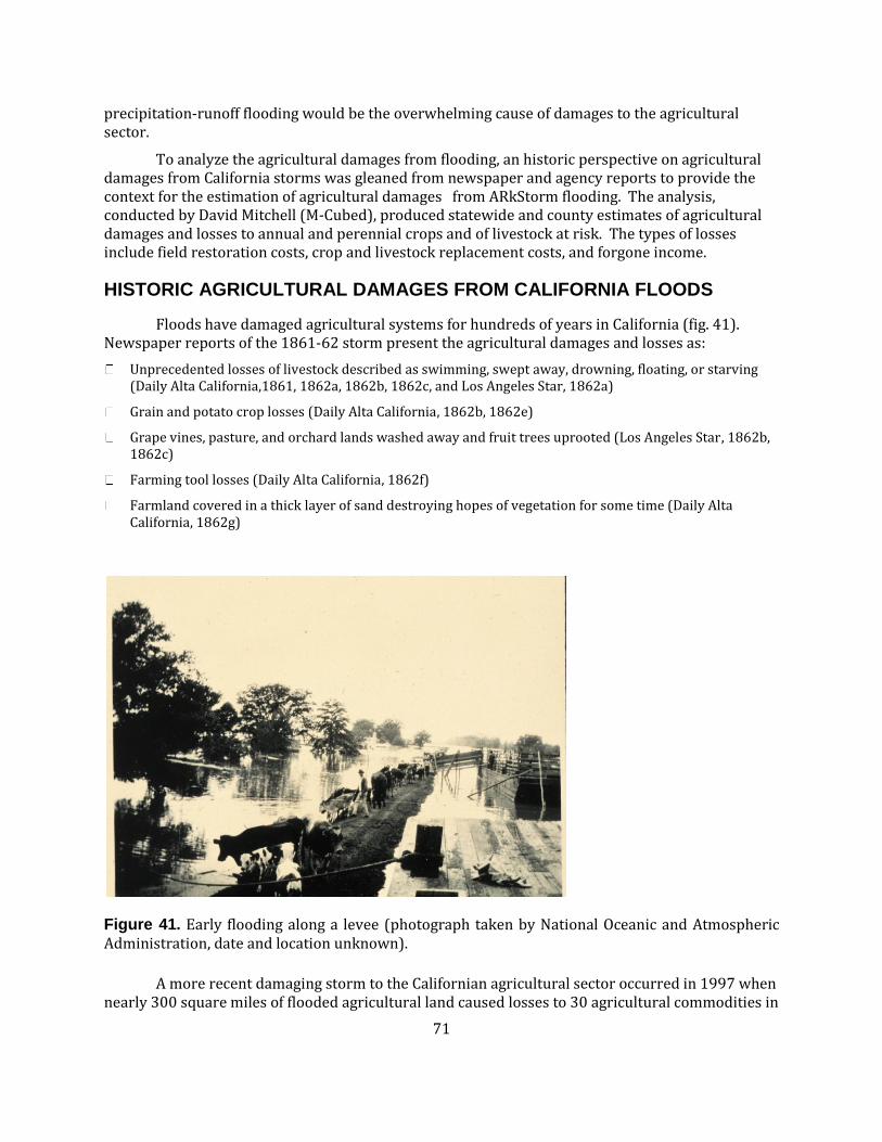
71

precipitation-runoff flooding would be the overwhelming cause of damages to the agricultural sector.

To analyze the agricultural damages from flooding, an historic perspective on agricultural damages from California storms was gleaned from newspaper and agency reports to provide the context for the estimation of agricultural damages from ARkStorm flooding. The analysis, conducted by David Mitchell (M-Cubed), produced statewide and county estimates of agricultural damages and losses to annual and perennial crops and of livestock at risk. The types of losses include field restoration costs, crop and livestock replacement costs, and forgone income.

HISTORIC AGRICULTURAL DAMAGES FROM CALIFORNIA FLOODS

Floods have damaged agricultural systems for hundreds of years in California (fig. 41). Newspaper reports of the 1861-62 storm present the agricultural damages and losses as:

Unprecedented losses of livestock described as swimming, swept away, drowning, floating, or starving (Daily Alta California,1861, 1862a, 1862b, 1862c, and Los Angeles Star, 1862a)

Grain and potato crop losses (Daily Alta California, 1862b, 1862e)

Grape vines, pasture, and orchard lands washed away and fruit trees uprooted (Los Angeles Star, 1862b, 1862c)

Farming tool losses (Daily Alta California, 1862f)

Farmland covered in a thick layer of sand destroying hopes of vegetation for some time (Daily Alta California, 1862g)

Figure 41. Early flooding along a levee (photograph taken by National Oceanic and Atmospheric Administration, date and location unknown).

A more recent damaging storm to the Californian agricultural sector occurred in 1997 when nearly 300 square miles of flooded agricultural land caused losses to 30 agricultural commodities in

72

more than 30 counties (California Department of Water Resources, 1997). The Flood Emergency Action Team (FEAT) final report (California Department of Water Resources, 1997) lists the economic losses as:

Crop losses totaled $107 million, with the largest losses being walnuts, wine grapes, winter wheat, and alfalfa.

Crop damage costs added another $49 million, with peaches, plums/prunes, wine grapes, and walnuts incurring the largest damage.

Damage to nurseries totaled $16 million

Livestock costs were another $12 million

Damages to farm infrastructure (irrigation systems, roads, buildings, and fences) totaled $109 million.

The most severely affected counties were Butte, Yuba, Stanislaus, Nevada, Sacramento, San Joaquin, and Sutter.

To summarize, five categories of agricultural damages can be identified from these reports: damages to annual crops, perennial crops (fig. 42), livestock, fields, and equipment. While flooding is the primary cause of these damages, reports on the 1986 storm (San Francisco Chronicle 8 Mar 1986) indicate agricultural damages and losses are further exacerbated by:

Bacterial diseases

Delays in pollination and maturity

Delays from pumping out agricultural fields.

For the ARkStorm scenario, we estimated field repair costs (that include costs of repair to roads, culverts, and irrigation systems), perennial and livestock replacement costs, and forgone annual and perennial crop income losses. Flood damage to agricultural building stock and contents (presumably including equipment and feed) was estimated at about $13 billion by using HAZUS-MH inventory and methodology. We were unable to consider the effects of bacterial diseases and delayed pollination. We were able to address the effects of further agricultural production delays resulting from the time to repair Delta levees and dewater islands.

73

Figure 42. Flooded vineyards, Guerneville, Calif., 2006, because of Russian River flooding (Photograph by A. Dubrowa for Federal Emergency Management Agency).

METHODOLOGY

ARkStorm agricultural damages and losses from flooding were estimated for the following commodity categories:

Annual crops

Oilseeds – which include seed crops such as sunflower.

Grains – which include wheat, barley, rice and other grains.

Vegetables and Melons

Fruits – which include strawberries and other annual fruit crops

Sugar Beets

All other annual crops, which include other forage and field crops

Perennial crops

Fruit trees – which include orchards and vineyards

Greenhouse and nursery – which include nursery stock, Christmas tree farms, and other greenhouse

crops1

Tree nuts - which include almonds, walnuts, pistachios, and other tree nuts

1 Greenhouse and nursery crops were included under perennial crops for simplicity.

74

All other perennial crops

Livestock operations

Dairy

Feedlot cattle

Poultry

Livestock damages pertain to livestock confined to feedlots, dairy farms, and poultry operations; we did not address potential losses of open range livestock.

The following data and methodologies were used to overlay agricultural commodity production on the flood map, calculate field repair and cleanup costs, and estimate agricultural damages.

Location, Extent, Depth, and Duration of Flooded Agricultural Land

DWR land-use survey data2 provided the spatial distribution of commodity production in 33 counties. The data specified one agricultural commodity for each area even if the commodity could be one of multiple crop types. GIS techniques were used to intersect acres of commodity production with the ARkStorm flood map attributes to produce the following information by county:

Total amount of county acreage by agricultural land use (for example. orchard, forage, feedlot)

Amount of county acreage by agricultural land use inundated under the ARkStorm flood scenario

Range of flood depth (in feet) and flood depth at midpoint of depth range by agricultural land use

Range of flood duration (in days) by agricultural land

Flood depth was set to the midpoint of the depth range for each land use class in a county. Low, mid-, and high flood durations were considered.

2 DWR land use surveys are done on a rotating basis. The survey data used for this study covered

the period 1993 to 2006. These land use surveys were performed by using aerial photographs and,

more recently, satellite imagery to define field boundaries. Most of the land use survey data are

entered directly into a digital map by using geographic information system (GIS) software on a

laptop computer. Georeferenced, orthorectified imagery is used as a backdrop, and the land use

boundaries are visible on top of the imagery. DWR staff visit and visually identify land uses on over

95 percent of the developed agricultural areas within each survey area. After the field work has

been completed and the maps have been checked for errors, a digital composite map of the survey

area is created from the work of individual surveyors. Using GIS software, digital maps of quads,

counties, water districts, and the DWR hydrologic planning units (Detailed Analysis Units) can be

overlaid on the land use data to develop acreage summaries of land use by areas. Digitized land use

survey data used for this study were downloaded at

www.water.ca.gov/landwateruse/lusrvymain.cfm.

75

Field Cleanup and Repair Costs

Floods may impact farmland by causing erosion and deposition of debris and sediment, damaging farm roads, and clogging drainage and irrigation ditches. Damages are likely to be highly variable, depending on the velocity of flood flows, as well as depth and duration of inundation. Field cleanup and repair costs used for this study are based on average per acre costs for cleanup and rehabilitation used by the U.S. Army Corps of Engineers (USACE) in the 2002 “Sacramento and San Joaquin River Basin Comprehensive Study” (U.S. Army Corps of Engineers, 2002). Costs were assumed to vary according to flood depth and duration as shown in table 9. Costs were updated to 2009 dollars.

Table 9. Field cleanup and repair cost assumptions.

[%, percent; USACE, U.S. Army Corps of Engineers; ft, foot; >, greater than]

Applied % of USACE Estimate

Flood Duration (Days)

Flood Depth (ft) 0-0.25 0.25-1.75 1.75-3 3-5 >5

0-2 0% 25% 50% 75% 100%

2-6 0% 50% 75% 100% 100%

>6 0% 100% 100% 100% 100%

$/Acre Cost

0-2 $0 $79 $157 $236 $314

2-6 $0 $157 $236 $314 $314

>6 $0 $314 $314 $314 $314

Damages to Annual Crops

Flooding of agricultural land can disrupt field preparation and planting, destroy crops in the ground, and disrupt or prevent harvesting. The extent and severity of impact depends on the season in which flooding occurs, the duration of inundation, and the type of crops inundated. Losses from spring and summer floods generally will be greater than from autumn and winter floods. Brief periods of inundation may result in only small damages if these floods occur after harvest and prior to spring planting. Longer periods of inundation occurring in the autumn and winter may prevent spring planting altogether. Spring and summer flooding, regardless of the duration of inundation, will destroy most field and row crops in the ground.

For this study, production losses for annual crops are based on the crop production loss models developed for the Delta Risk Management Strategy Phase 1 Report (California Department of Water Resources, 2008). The crop loss values in this model were calculated by using Delta crop revenue and cost estimates prepared by DWR and monthly distributions of crop production costs

76

and revenues developed for the Sacramento and San Joaquin River Basins Comprehensive Study (California Department of Water Resources, 2005 U.S. Army Corps of Engineers, 2002). The model calculates the difference between lost harvest revenue and avoided production expenses as a function of the month in which a flood is assumed to occur. For this study, flooding was assumed to occur primarily in February.3 In addition, the models make the following assumptions about crops in the ground and planting of crops for next season:

Three months is required following dewatering for cleanup and rehabilitation before fields can be

prepared for planting.4

Spring/summer crops will not be planted if a field has not been dewatered and repaired by the end of March.

Flooding occurring in January and February will destroy winter grain crops.

Given the above assumptions about lead times required for dewatering and field cleanup and rehabilitation, the ARkStorm flood scenario was assumed to disrupt the planting of truck crops and processing tomato crops, and winter grain crops, but not the planting or harvest of rice, corn, and other field crops. Average losses in 2009 constant dollars for flooded processing tomato and truck crop acreage are $424 and $1,479 per acre, respectively. The average loss for winter grain crops is $285 per acre. Crop income losses and field repair costs are assumed to be incurred in the same six-month period in which the flood occurs.

Damages to Perennial Crops

Prolonged inundation may result in extensive damage or death of permanent orchard, vineyard and hay crops. Damages result largely from anaerobic soil conditions. In addition anoxic conditions in the soil can lead to the release of toxic substances such as manganese. A review of the literature provided limited information on the effects of prolonged inundation on various crop types (California Department of Water Resources, 2008).

For this study, production losses for perennial crops are based on the crop production loss models developed for the Delta Risk Management Strategy (California Department of Water Resources, 2005). These models assume that perennial crops inundated for 14 days or more would be killed by anaerobic soil conditions caused by standing water. Estimated damages are equal to the replacement cost of the crop plus the foregone production net income from crop production during the period of crop reestablishment. Damages are calculated in six-month increments. We assume field repair costs are incurred in the first six months; crop reestablishment costs are incurred in the six month period following the flood in which the crop would typically be planted; and net crop income losses are incurred in the six monthly periods following the flood in which the crop would typically be harvested.

Orchard crops are assumed to have an average reestablishment cost of $9,100 per acre and to require 4 years to reestablish. Annual net crop income loss is assumed to average $3,900 per

3 Under the ARkStorm scenario flooding commences in middle to late January in northern California

and early February in Southern California. February damage estimates from the crop models were

considered to be most representative.

4 This assumption is based on the experience with Jones Tract in the Sacramento/San Joaquin Delta.

77

acre in the flood year and $2,600 per acre thereafter.5 Vineyard crops are assumed to have an average reestablishment cost of $11,400 per acre and to require 3 years to reestablish. Annual net crop income loss is assumed to average $3,700 per acre in the flood year and $3,400 per acre thereafter. Forage crops (primarily alfalfa) are assumed to have an average reestablishment cost of $640 per acre and to require 1 year to reestablish. Annual net crop income loss is assumed to average $530 per acre.

Damages to Livestock

Damages to livestock confined to feedlots, dairy farms, and poultry operations are based on the replacement cost of livestock at risk of death by drowning. The replacement costs estimation assume the livestock are lost, though some producers may be able to mitigate losses by temporarily relocating some or all of their stock. Livestock inventory and replacement cost estimates are taken from U.S. Department of Agriculture (USDA) Livestock Review reports for California. Livestock inventories were allocated across counties in proportion to each county’s share of statewide feedlot, dairy, and poultry farm acreage, which was determined from the DWR land use survey data.

Flood depths of 6 feet or greater were assumed to place feedlot, dairy, and poultry livestock at substantial risk of death by drowning.6 The number of head at risk was calculated by multiplying the fraction of feedlot, dairy, and poultry farm acreage in each county with a flood depth of 6 feet or greater by the county livestock inventory. This calculation yielded the estimated number of livestock potentially at risk under the ARkStorm flood scenario.

The value at risk is calculated by multiplying the number of livestock potentially at risk by the replacement cost per head. The average replacement cost for feedlot cattle is based on the inventory of cows, heifers, steers, and calves and the respective value per head. The average value used in this study is $678 per head.7 Replacement costs for dairy cows and poultry come directly from USDA. Dairy cow replacement cost used in this study is $1,300 per head. Poultry replacement cost is $2.60 per head. Both estimates are based on 2009 prices received by California farmers. Livestock replacement and field repair costs are assumed to be incurred in the same six-month period in which the flood occurs.

5 The higher net income loss in the flood year is because of production costs incurred prior to the

flood event. In subsequent years these production costs can be avoided.

6 The rationale for a flood depth threshold of 6 feet is that livestock operators would have more

opportunity to move livestock to safe ground or let livestock wait out the flood at lesser depths;

whereas, depths of 6 feet or more would likely pose an existential threat to most livestock and

likely would entail mandatory evacuations, which would limit the ability of operators to move

livestock to safe ground.

7 This is based on 2008 marketing year prices reported by USDA.

78

ARkSTORM AGRICULTURAL DAMAGE ESTIMATES

Damaged Land

Damaged lands were defined in relation to the following damage parameters: any flooding of annual crop land was assumed to result in damage to crops already in the ground; damage to perennial crop production is assumed in areas where flood waters do not recede for 14 or more days; and significant damage to livestock production is assumed in areas where flood depth is 6 feet or more.

The percent of land area in annual crops, perennial crops, and livestock production significantly damaged by flooding is summarized in table 10. Overall, the ARkStorm flood scenario results in significant damage to about 23 percent of acreage in annual crop, 5 percent of dairy, feedlot, and poultry livestock production, and 5 percent of perennial crop production. Comparable results by county and commodity category are available in appendix A. The percent damage varies greatly by county, with counties in the northern part of the San Joaquin Valley and southern part of the Sacramento Valley experiencing the most damage. Areas within the San Joaquin-Sacramento Delta are especially vulnerable to damage.

Table 10. Acres of significantly damaged agricultural lands. Values pertain to flooded annual crop lands, perennial crop lands with more than 14 days of flooding, and livestock areas with flood depth greater than 6 feet.

[%, percent]

Commodity Acres production

(thousands)

Acres significant damage

(thousands)

Percent

Annual crop 18,582 4,324 23%

Perennial crop 5,673 261 5%

Livestock 285 13 5%

Statewide Agricultural Damages

Economic losses accrue from costs of field cleanup, and repair; perennial crop and livestock replacement; and forgone annual and perennial crop income. In the case of annual crops, foregone crop income is the difference between the harvest value of the crops destroyed and avoided production expenses. In the case of perennial crops (orchards and vineyards), foregone crop income is the sum of net crop income losses during the period of crop re-establishment. Figure 43 presents the estimated state losses of $3.75 billion (2009 constant dollars) for the low-end flood duration. Although there is 16 times more significantly damaged annual crop land than significantly damaged perennial crop land, most of the losses pertain to perennial crops for two reasons: reestablishment of these crops incurs replacement costs and multiple years of forgone income until the crop bears fruit. The high-end flood duration estimate increases annual, perennial, and livestock losses by 25 percent, 100 percent, and 1 percent, respectively, revealing the sensitivity of perennial crops to longer flood durations.

79

Figure 43. State agricultural damages to annual and perennial crops and livestock.

Table 11 through table 13 display the statewide damages by commodity category under annual and perennial crops and livestock for the low, mid-, and high flood durations. For the annual crops (table 11), about 50 percent of the losses pertain to grains and 25 percent to vegetables and melons. For the perennial crops (table 12), the damages are dominated by fruit tree damages; fruit tree (including vineyard) damages represent about 65 percent of the perennial crop damages. Damages to nut trees comprise about 25 percent of total damages to perennial crops and damages to forage crops (alfalfa) and nursery crops about 10 percent. Damages to perennial crops are spread over a 5-year reestablishment period, with about 70 percent of the total occurring in the first two years and 30 percent in the 3 subsequent years. The first two years of damages primarily are because of field damage and reestablishment costs while damages in the latter three years accrue from forgone crop income during the nonbearing period of reestablished orchards and vineyards. Differences in crop income losses across low, mid, and high flood duration occur when the flood duration causes further damage as is the case for perennial crop damage that is sensitive to greater than 14 days of flooding. For the livestock damages (table 13), just over 80 percent of the livestock replacement costs apply to dairy because the cost per head of dairy is twice that of feedlot herd and more dairy lands are significantly damaged.

80

Table 11 Statewide damages to annual crops for low, mid and high flood durations. All amounts are in millions of 2009 dollars.

[low, mid, high are flood duration designations]

Crop Category Crop Income Losses Field Damages Total Damages

Low Mid- High Low Mid- High Low Mid- High

All Other Crops $0.0 $0.0 $0.0 $56.7 $79.0 $92.2 $56.7 $79.0 $92.2

Fruits $52.5 $53.0 $53.0 $30.1 $37.0 $38.9 $82.6 $90.0 $91.9

Grains $85.3 $85.3 $85.3 $188.5 $244.7 $253.0 $273.8 $330.0 $338.3

Oilseeds $0.0 $0.0 $0.0 $2.3 $3.1 $3.1 $2.3 $3.1 $3.1

Sugar Beets $0.0 $0.0 $0.0 $4.6 $5.3 $5.7 $4.6 $5.3 $5.7

Veg/Melon $110.9 $129.4 $129.4 $20.4 $25.6 $26.9 $131.4 $155.0 $156.3

Total $248.7 $267.7 $267.7 $302.6 $394.7 $419.8 $551.3 $662.4 $687.5

Table 12. Statewide damages to perennial crops over 5-year reestablishment. All amounts are in millions of 2009 dollars.


Crop

Category

Crop income losses Field damages and crop

replacement cost

Total Damages


Fruit

Trees

$1,06

1.8

$1,06

1.8

$2,09

5.9

$871.2 $888.6 $1,591.0 $1,93

3.0

$1,95

0.4

$3,68

6.9

Nut Trees $464.

7

$464.

7

$1,27

4.6

$327.3 $340.2 $858.0 $791.

9

$804.

9

$2,13

2.6

Peren.

Forage

$79.8 $79.8 $136.

1

$179.6 $214.0 $288.2 $259.

5

$293.

8

$424.

3

Greenhou

se

$9.4 $9.4 $19.3 $7.3 $7.9 $14.3 $16.7 $17.3 $33.6

Total $1,61

5.7

$1,61

5.7

$3,52

5.9

$1,385.4 $1,450.7 $2,751.5 $3,00

1.0

$3,06

6.3

$6,27

7.4

81

Table 13. Statewide damages to livestock. All amounts are in millions of 2009 dollars.


Livestock

Category*

Livestock Losses Field Damages** Total Damages


Dairies $110.6 $110.6 $110.6 $1.5 $2.3 $2.4 $112.1 $112.9 $113.0

Feedlots $22.2 $22.2 $22.2 $0.2 $0.4 $0.4 $22.4 $22.6 $22.6

Poultry $1.3 $1.3 $1.3 $0.4 $0.6 $0.7 $1.6 $1.9 $2.0

Total $134.1 $134.1 $134.1 $2.0 $3.2 $3.5 $136.1 $137.3 $137.6

* Does not include possible damages to free range livestock.

**Does not include damages to structures (for example, barns) or contents of structures (for

example, milking equipment).

County Agricultural Damages

County results of annual and perennial crop and livestock losses were mapped for the first year and subsequent years (fig. 44 through fig. 47). The losses extend beyond the first year for perennial crops only. In the case of perennial crops, field repair costs are assumed to occur in the first six months, but crop income losses and reestablishment costs extend into the future, depending on the season in which the crop typically would be reestablished and the number of years until the crop would be bearing. The maps show the variation of losses across counties and the distribution of losses to commodities. About $140 million of the annual crop losses (about one third of the total for annual crops) occur in San Joaquin County followed by $55 million of annual crop losses in Kings County. San Joaquin County incurs about half of the perennial crop damages, followed by Sacramento and Yolo Counties. For livestock damages, again, the damages are concentrated in San Joaquin with almost half of the livestock damages. In contrast to crops, southern California counties are relatively more affected by livestock damages with $22 million in Riverside County and $13 million in San Diego County for replacement of dairy and livestock feedlot cattle. See appendix A for further details on the field costs, replacement costs, and forgone income losses by commodity and by county.

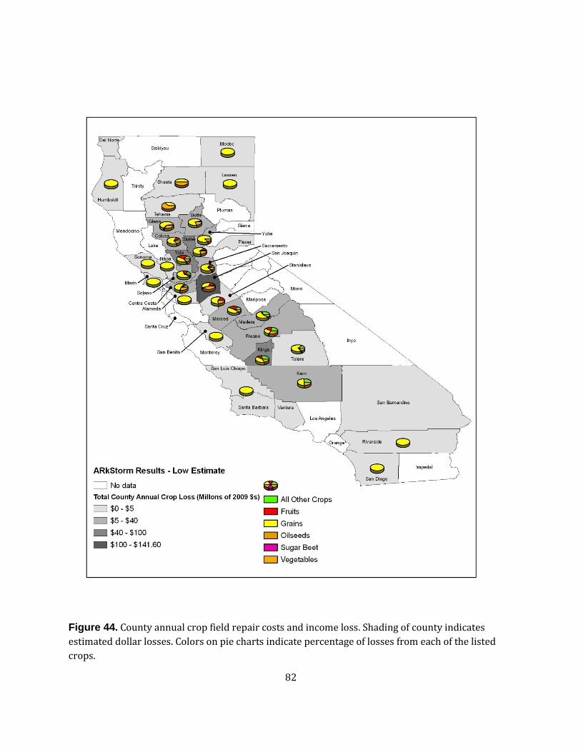
82

Figure 44. County annual crop field repair costs and income loss. Shading of county indicates

estimated dollar losses. Colors on pie charts indicate percentage of losses from each of the listed

crops.

83

Figure 45. County perennial crop replacement and income loss (first year). Shading of county indicates estimated dollar losses. Colors on pie charts indicate percentage of losses from each of the listed crops.

84

Figure 46. County perennial crop income loss (subsequent years). Shading of county indicates estimated dollar losses. Colors on pie charts indicate percentage of losses from each of the listed crops.

85

Figure 47. Livestock replacement cost. Shading of county indicates estimated dollar losses. Colors on pie charts indicate percentage of losses from each of the types of livestock listed.

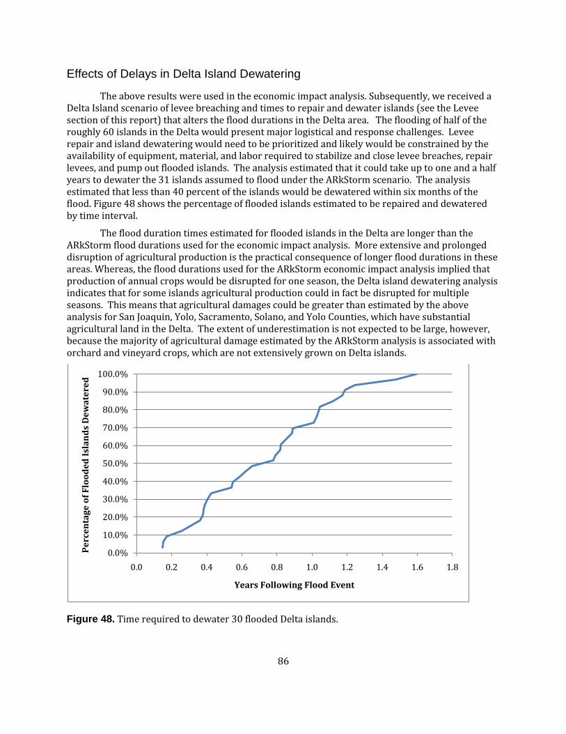
86

Effects of Delays in Delta Island Dewatering

The above results were used in the economic impact analysis. Subsequently, we received a Delta Island scenario of levee breaching and times to repair and dewater islands (see the Levee section of this report) that alters the flood durations in the Delta area. The flooding of half of the roughly 60 islands in the Delta would present major logistical and response challenges. Levee repair and island dewatering would need to be prioritized and likely would be constrained by the availability of equipment, material, and labor required to stabilize and close levee breaches, repair levees, and pump out flooded islands. The analysis estimated that it could take up to one and a half years to dewater the 31 islands assumed to flood under the ARkStorm scenario. The analysis estimated that less than 40 percent of the islands would be dewatered within six months of the flood. Figure 48 shows the percentage of flooded islands estimated to be repaired and dewatered by time interval.

The flood duration times estimated for flooded islands in the Delta are longer than the ARkStorm flood durations used for the economic impact analysis. More extensive and prolonged disruption of agricultural production is the practical consequence of longer flood durations in these areas. Whereas, the flood durations used for the ARkStorm economic impact analysis implied that production of annual crops would be disrupted for one season, the Delta island dewatering analysis indicates that for some islands agricultural production could in fact be disrupted for multiple seasons. This means that agricultural damages could be greater than estimated by the above analysis for San Joaquin, Yolo, Sacramento, Solano, and Yolo Counties, which have substantial agricultural land in the Delta. The extent of underestimation is not expected to be large, however, because the majority of agricultural damage estimated by the ARkStorm analysis is associated with orchard and vineyard crops, which are not extensively grown on Delta islands.

Figure 48. Time required to dewater 30 flooded Delta islands.

0.0%

10.0%

20.0%

30.0%

40.0%

50.0%

60.0%

70.0%

80.0%

90.0%

100.0%

0.0 0.2 0.4 0.6 0.8 1.0 1.2 1.4 1.6 1.8

Pe

rce

nta

ge

of

Flo

od

ed

Isl

an

ds

De

wa

tere

d

Years Following Flood Event

87

SUMMARY

The ARkStorm winter storm agricultural damages are an order of magnitude greater than 1997 flood damages. Statewide damages to crops, livestock, and fields were estimated to range between $3.7 and $7.1 billion.8 Destruction of perennial orchard and vineyard crops accounted for most of the estimated agricultural production losses. We note that these perennial crop losses may have been underestimated because of the use of old survey information that in some areas may be more than 10 years old. Recent crop shifts away from field and forage crops toward fruit and vegetable crops, and especially toward orchards and vineyards may have affected the estimate. A quick look at the county agricultural reports of the 3 most-affected counties (Sacramento, San Joaquin, and Yolo) indicates that perennial crop acreage has increased by more than 20 percent in the last 10 years (Stephen Hatchett, Western Research Economics, 2010, written commun.). Damages to farm structures and equipment, were estimated separately at $13 billion by using the HAZUS-MH inventory and methodology.

Like the 1997 storm, San Joaquin and Sacramento Counties are among the counties most severely affected by the ARkStorm scenario, but damages in Yola, Solano, and Kings Counties are relatively more severe. Agricultural production in the Delta, much of which occurs on deeply subsided islands protected by increasingly fragile levees, appears to be particularly at risk.

MITIGATING AGRICULTURAL DAMAGES

It is not possible to move crops and farm structures out of harm’s way during a flood. It is possible to provide buffers and barriers between these assets and flood waters. Thus flood protection for most agricultural assets depends on a broader set of land use and flood risk mitigation policies. In the case of livestock, given adequate advance warning and livestock relocation contingency plans, mobilization and relocation may be possible. Dairy is the most problematic because of the need for milking facilities. The California dairy industry has made some effort in recent years, in conjunction with the California Department of Food and Agriculture, to implement a formal emergency alert system that could be used to provide early warning in the event of a fast moving disease outbreak9 or pending natural disaster, such as the threat of

8 We have estimated repair and replacement costs of damaged assets and infrastructure. This

estimate is consistent with damage estimates in the rest of the ARkStorm scenario report. Economic

damages to landowners pertain to earlier replacement of perennial crops and livestock. Supposing

perennial crops are replaced two-fifths through the useful life, and by using a real discount rate of 3

percent, the present value reestablishment cost is about 70 percent of the cost calculated simply as

a new capital cost plus several years of no income.

9 For example, experts estimate that in the case of an outbreak of Foot and Mouth Disease in

California, each hour that the disease goes unrecognized could cost the dairy industry between one

and three million dollars. (Dr. Michael Payne, Program Director, California Dairy Quality Assurance

Program, written commun., 2010.)

88

flooding.10 However, progress on the system has been stymied by industry concerns about how producer information needed to implement the system, some of which the dairy associations consider proprietary, would be safeguarded.

Even with a robust alert system in place, livestock producers also must be able to act on the information. Mobilizing and relocating livestock in large numbers presents obvious logistical challenges. Adequate transportation has to be available to move the livestock and the livestock have to have some place to go. The success of mobilizing and relocating large numbers of livestock on short notice will depend almost entirely on having emergency relocation plans and the resources necessary to implement those plans already in place. Our research suggests that planning in this area is not very far advanced. The level of contingency planning among livestock producers in not known and, likely, many do not have flood emergency response plans in place, according to at least one industry expert (M. Payne California Dairy Quality Assurance Program, written commun., 2010). Floods are rare events and responses are too often handled on the fly.11 This may work when only a few isolated producers are affected, but such a strategy is sure to fail under a scenario such as ARkStorm.

Animal emergency response plans reside in county plans to varying degrees, but moving stock at the regional scale has not been examined. This response plan is on the agenda for the upcoming Golden Guardian 2011 exercise. After the 1997 storm, the California Animal Emergency Response System (CARES) was established. This system is being revitalized by the California Department of Food and Agriculture (CDFA).12 “CARES will coordinate resources and decisions once an incident escalates to a state-level emergency; the CARES Plan is not intended to supersede local government plans but to assist them as they exhaust their resources” (California Department of Food and Agriculture, 2000).

RESEARCH NEEDS RELATED TO AGRICULTURAL DAMAGES

We neglected estimation of livestock disposal costs for livestock at risk. In addition, the agriculture sector will not only be directly affected by flood damages to crops and livestock, but also by associated power outages, well contamination, and access limitations. We capture sector interdependencies in the economic impact analysis. However, we note that further disruptions from

10 The proposed alert system had the capacity to send out 48,000 emails in 2 minutes, and provide

additional follow-up through automated phone message recordings. (Dr. Michael Payne, Program

Director, California Dairy Quality Assurance Program, written commun, 2010.)

11 This situation is not unique to California. A recent news article tells the story of a Freeport,

Illinois, dairy farm along the Pecatonica River that would have lost 500 head of cattle to rising flood

waters but for the fact that a neighboring dairy in the process of doubling its operation had recently

completed construction of new barns, which were temporarily standing empty. Had these barns

not been available and had neighbors not pitched in to move the cattle, the herd may have been lost.

The story illustrates the inherent challenges of moving even a relatively small number of livestock

on short notice. (http://gazettextra.com/news/2010/jul/29/larson-acres-provides-home-flooded-

illinois-cows/ accessed on August 6, 2010.)

12 John Rowden, California Department of Food and Agriculture,. written commun., August 17, 2010.

http://gazettextra.com/news/2010/jul/29/larson-acres-provides-home-flooded-illinois-cows/�

http://gazettextra.com/news/2010/jul/29/larson-acres-provides-home-flooded-illinois-cows/�

89

aqueduct damage and salinity were not studied, although, it is believed that initially the quantity of precipitation runoff will keep salinity at bay. Conversely, agricultural losses would indirectly affect other industrial sectors. The effects of crop losses (not livestock losses) on other sectors were evaluated in the ARkStorm economic impact analysis which allows for commodity price responses.

Finally, insurance payments and federal disaster payments are resilience strategies that would enable the recovery of the California agricultural sector, but the breakdown of insured and uninsured losses was not evaluated.

Building and Content Repair Costs

PROPERTY-DAMAGE METHODOLOGY

We use the HAZUS-MH methodology, its building exposure data, and its flood and wind vulnerability functions to estimate wind and flood damage to the general building stock resulting from the ARkStorm. However, we performed the loss calculations outside the HAZUS-MH software because (1) the ARkStorm flood map could not be readily imported into the HAZUS-MH flood module and (2) because the HAZUS-MH wind module does not include California. We adapted the Florida wind vulnerability and fragility functions for use in California by shifting those functions to account for lower design wind speeds (and, therefore, likely higher wind vulnerability) in California. We estimate damage and loss at each census block and by each of the 33 occupancy classes in HAZUS-MH, and then we aggregated to the state level. The full methodology is documented in Olsen and Porter (2010).

The HAZUS-MH methodology begins with a description of the inventory of assets exposed to loss. The inventory is characterized by estimates of the number of buildings, building area, building replacement cost (the cost to build a functionally and architecturally similar building at the same location, if the existing building were not there), content replacement cost (including furnishings, fixtures, equipment, and business inventories), and the number of building occupants at three times of day, based on working patterns. HAZUS-MH provides these quantities by census block and occupancy class. The estimates begin with data from the Census of Population and Housing and from the Economic Census. These and other sources provide estimates of the number of people living or working in a census block. The estimated total building area by census block is the product of the number of people and estimates of the per person square footage of the buildings these people occupy. Companies that estimate construction costs provide estimates of the replacement costs of the buildings (again, the cost to construct the buildings new, often estimated on a per-square-foot basis in construction cost manuals). Using insurance and other rules of thumb, one can then estimate the content value as a multiplicative factor of building value. The distributions of these building inventory characteristics by structure type can be estimated by using engineering experience and, in some cases, information from building departments and the insurance industry.

The building inventory as defined by HAZUS-MH is then overlain on the ARkStorm scenario maps of flood depth and wind speed (fig. 8, and fig. 9). When there is an asset in the inventory that is exposed to flooding or damaging winds, we find the damage ratio from a vulnerability function for that asset’s structure type. A vulnerability function is a relationship between an environmental excitation—here, flood depth or wind speed—and the ratio of repair cost to replacement cost, known as the damage ratio. We use unmodified HAZUS-MH flood vulnerability functions, but we modify the HAZUS-MH wind vulnerability functions as described in a subsequent paragraph. Figure 49 shows flood vulnerability functions for several structural types of residential occupancy. HAZUS-MH vulnerability functions provide the mean, or expected value, of the damage ratio given the

90

environmental excitation; the uncertainties in the vulnerability functions are not estimated. We calculate the expected loss by multiplying the damage ratio by the value exposed for each combination of census block, occupancy class, and structure type. Adding up the loss for each combination leads to an estimate of aggregate repair cost.

Figure 49. Sample HAZUS-MH flood vulnerability functions showing damage ratio for different types of single-family dwellings.

Equation (3) states mathematically what we have just described. L represents the expected value of loss, such as building repair cost. The three large Greek sigma characters mean ”sum over” or ”add up” and the letters beneath them—i, j, and k—are counters, referring respectively to census

blocks (i), occupancy classes (j), and structure types (k). The term , ,i j kV

represents the estimated

value exposed to loss in census block i, occupancy class j, and structure type k. , ,i j kV

is multiplied

by ,j k iy x, which is the vulnerability function evaluated at location i. In other words, ,j k iy x

is the mean damage ratio for an asset of occupancy class j and structure type k, when exposed to the environmental excitation x experienced by census block i.

, , ,i j k j k i

i j k

L V y x

(3)

91

We modified the wind vulnerability functions encoded in HAZUS-MH for use in California. HAZUS-MH does not have a wind model for California, so we used vulnerability functions from its Florida hurricane model. The International Building Code defines the primary wind speed to be used for the design of buildings (known as the basic wind speed) as 85 mph for sites in California and as 130 mph ± 20 mph for sites in Florida (American Society of Civil Engineers, 2006). We assume that a California building exposed to 85 mph winds would be damaged to the same extent as a similar Florida building exposed to 130 mph winds. Thus, we shift the wind speed axis of the Florida vulnerability functions to account for the lower basic wind speed in California when compared to Florida.

PROPERTY-DAMAGE SCENARIO

Based on the methodology described in the previous section, the estimated repair cost for flood-induced building damage is about $200 billion, which is equivalent to approximately 7 percent of the HAZUS-MH estimate of the replacement cost of all buildings in California ($2.7 trillion), or 2-3 years of statewide construction spending at 2006-2007 rates (about $75 to $100 billion per year). Flood-related content losses are estimated to contribute another $100 billion. The reason for these very high flood-related losses is evident when examining the flood maps in detail. Figure 50 through figure 53 show extensive inundation of urban areas in Sacramento, Stockton, the San Jose area, and Los Angeles and Orange Counties.

Using the HAZUS-MH methodology, inventory, and vulnerability functions, we first calculated flood-related content losses as roughly equal to flood-related building losses. However, this result seemed unreasonable: the content losses seemed too high—perhaps by a factor of two—relative to the building losses. To check whether the content losses ought to roughly equal building losses, we examined National Flood Insurance Program claims documented in a FEMA Flood Mitigation Assistance database. The Flood Mitigation Assistance grants in the database mostly were dated between 1996 and 2003. We examined all claims where there were nonzero building losses and nonzero content losses. There were 485 such claims, dated between 1977 and 2001. These claims totaled about $8.6 million for building losses and $5.1 million for content losses, or roughly a $0.60 content loss per $1.00 of building loss. These claims data reinforce our doubts about the content losses first estimated in the ARkStorm scenario. The 0.60:1.00 ratio implied by the Flood Mitigation Assistance data is close to an upper boundary because the database showed many properties with repetitive losses where some, but not all, of the claims included content losses. These data suggest that there are properties with both structure and content coverage that experienced claims with structure loss but not content loss. Such claims are not included in the $8.6 and $5.1 million loss totals. If these claims were added to the totals that would increase the $8.6 million figure but not the $5.1 million figure. With this evidence in mind, we somewhat arbitrarily reduced by half the content losses estimated with the HAZUS-MH methodology and data, and we reported that value in the above paragraph.

HAZUS-MH data on California census blocks include classification as riverine or coastal. The loss from flood damage to building structures in all coastal census blocks is $29 billion, and the loss from flood damage to building structures in all riverine census blocks is $164 billion. This loss in coastal areas is 15 percent of the total flood loss from structural damage. Note, however, that we calculated all property losses from the flood map derived from rainfall runoff, not from the coastal inundation study in Southern California.

92

Figure 50. ARkStorm hypothetical flooding in Sacramento.

Figure 51. ARkStorm hypothetical flooding in Stockton.

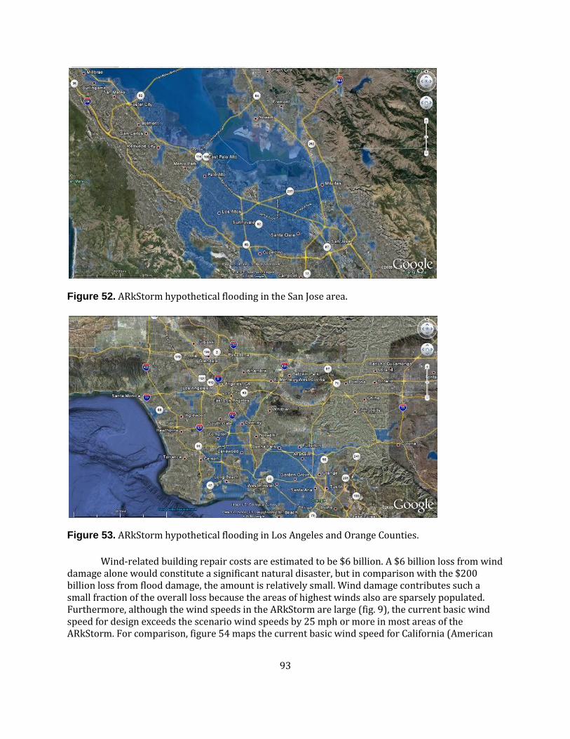
93

Figure 52. ARkStorm hypothetical flooding in the San Jose area.

Figure 53. ARkStorm hypothetical flooding in Los Angeles and Orange Counties.

Wind-related building repair costs are estimated to be $6 billion. A $6 billion loss from wind damage alone would constitute a significant natural disaster, but in comparison with the $200 billion loss from flood damage, the amount is relatively small. Wind damage contributes such a small fraction of the overall loss because the areas of highest winds also are sparsely populated. Furthermore, although the wind speeds in the ARkStorm are large (fig. 9), the current basic wind speed for design exceeds the scenario wind speeds by 25 mph or more in most areas of the ARkStorm. For comparison, figure 54 maps the current basic wind speed for California (American

94

Society of Civil Engineers ,2006). In fig. 54, the basic wind speed is 85 mph (38 meters per second) in California. Shaded areas denote special wind regions where unusual wind conditions exist.

We do not calculate the loss to building contents from wind damage. The wind vulnerability functions for contents cannot be extracted from the HAZUS-MH software or documentation for most occupancy classes. Nonetheless, it seems reasonable that content losses caused by wind damage would be negligible in comparison to content losses from flood damage. Again, the areas of highest wind speeds have a low potential for property loss.

Figure 54. Basic wind speed map for California (American Society of Civil Engineers, 2006, figures 6-1) and adjoining states, showing zones where basic wind speed for design is 85 miles per hour (38 meters per second) and 90 miles per hour (40 meters per second).

Nearly one-quarter of the total building square footage in California is affected by flooding in ARkStorm, with little variation of this ratio between occupancy classes (fig. 55) Most flooded buildings are not a total loss, but rather experience damage requiring repair costs between 10 percent and 50 percent of replacement cost. Residential buildings dominate the flood-related building repair costs, as shown figure 56. Residential buildings (labeled "RES" in Figure 56) account for 81 percent of the total estimated flood-induced building repair costs and 96 percent of wind-related losses. Commercial ("COM") buildings account for 13 percent and 2 percent of loss from flood and wind damage, respectively. The modest balance of loss is from damage to buildings with the following occupancy classes: industrial ("IND"), religion or nonprofit ("REL"), governmental ("GOV"), education, ("EDU") and agriculture. ("AGR"). Table 14 lists property losses by county, divided according to flood- or wind-related loss.

95

Figure 55. Fraction of building square footage affected by ARkStorm flooding for buildings in the occupancy classes agriculture, commercial, education, governmental, industrial, religion or nonprofit, and residential.

RESILIENCY AND RESEARCH NEEDS FOR BUILDING DAMAGE

Although the purpose of the work described in these sections is to estimate property losses, a few obvious opportunities for research and improved resiliency present themselves:

Consider mold in post-flooding inspections. This scenario disaster has a large number of flooded buildings, which raises questions about how safety inspections would be performed after a real-world California flood. A standard methodology from the Applied Technology Council (ATC)—known as ATC-45—exists for performing these inspections and posting the safety of buildings (Applied Technology Council, 2004). The ATC-45 methodology establishes the level of safety based on observed damage resulting from: inundation; hydrostatic and hydrodynamic forces; waves; erosion and scour; and various kinds of wind damage. After Hurricane Katrina in 2005, building inspectors in New Orleans performed safety inspections for more than 100,000 buildings. This experience showed that mold also can be a source of damage resulting from flooding, and can endanger occupants’ safety. While mold is a more modest concern after a California winter storm, it may be worthwhile to consider procedures that address mold in the ATC-45 methodology.

Expand training for ATC-45. A large cadre of structural engineers and others has been trained to perform post-earthquake safety inspections. Training for inspection of flood and wind damage in California has been more modest.

Examine flood warning systems. Research in the late 1960s by the U.S. Army Corps of Engineers, New York District, suggested that 48 hours of advanced warning could reduce riverine flood damage in the Passaic River Basin in New Jersey by up to 35 percent. The developers of the HAZUS-MH flood module observed that this was an upper boundary and that in practice the savings would probably be less than this hypothetical maximum. If 48 hours of warning could reduce property losses by 10 percent in the ARkStorm. This reduction is equivalent to at least $30 billion, a significant avoided loss.

Develop California wind vulnerability functions.

0%

10%

20%

30%

40%

50%

AG

R

CO

MED

UG

OV

IND

REL

RES

Occupancy group

Fra

ctio

n o

f ar

ea a

ffec

ted

96

Continue to improve the building inventory. Special attention is needed for the presence or absence of

basements in single-family residences.

Figure 56. Contribution to $200 billion in flood-related building repairs (left), and $6 billion in wind-related building repairs (right) for buildings in the occupancy classes agriculture, commercial, education, governmental, industrial, religion or nonprofit, and residential.

97

Table 14. ARkStorm property loss by county. $1,000s, on replacement-cost basis. [values do not sum exactly to the total shown because of rounding]

County Flood Wind County Flood Wind Alameda 14,000,000 270,000 Orange 50,000,000 22,000 Alpine 3,300 3,300 Placer 120,000 120,000 Amador 10,000 10,000 Plumas 19,000 20,000 Butte 320,000 61,000 Riverside 1,600,000 580,000 Calaveras 9,300 9,600 Sacramento 29,000,000 92,000 Colusa 230,000 9,100 San Benito 320,000 45,000 Contra Costa 16,000,000 430,000 San Bernardino 840,000 850,000 Del Norte 220,000 2,600 San Diego 25,000,000 24,000 El Dorado 120,000 120,000 San Francisco 990,000 180,000 Fresno 66,000 18,000 San Joaquin 22,000,000 72,000 Glenn 29,000 11,000 San Luis Obispo 440,000 86,000 Humboldt 1,400,000 5,100 San Mateo 11,000,000 380,000 Imperial 5,500 6,100 Santa Barbara 1,300,000 73,000 Inyo 47,000 59,000 Santa Clara 40,000,000 59,000 Kern 220,000 140,000 Santa Cruz 66,000 62,000 Kings 44,000 13,000 Shasta 270,000 49,000 Lake 14,000 16,000 Sierra 5,300 5,400 Lassen 60,000 31,000 Siskiyou 7,400 7,700 Los Angeles 46,000,000 580,000 Solano 7,000,000 130,000 Madera 29,000 190 Sonoma 5,500,000 86,000 Marin 8,500,000 72,000 Stanislaus 140,000 55,000 Mariposa 1,600 1,300 Sutter 2,400,000 41,000 Mendocino 1,400,000 26,000 Tehama 130,000 22,000 Merced 65,000 18,000 Trinity 990 79 Modoc 23,000 7,100 Tulare 17,000 2,200 Mono 44,000 47,000 Tuolumne 6,900 7,300 Monterey 280,000 280,000 Ventura 4,300,000 34,000 Napa 2,000,000 33,000 Yolo 3,800,000 47,000 Nevada 33,000 33,000 Yuba 1,000,000 24,000 Total 300,000,000 5,500,000

DEMAND SURGE

If an event, such as an earthquake or flood, damages a very large number of properties, the cost to repair a given amount of damage at a particular property can be greater than to repair the same damage if fewer other properties were damaged. This increased repair cost is known as “demand surge,” and is a poorly understood socioeconomic phenomenon of large-scale natural disasters. Demand surge has caused estimated cost increases of 20 percent (for example, the 1994 Northridge Earthquake; Kuzak and Larsen, 2005) to 50 percent (for example, Cyclone Larry in 2006; Australian Securities and Investments Commission, 2007) in past catastrophes, and the ARkStorm would certainly measure among the largest of these catastrophes in terms of absolute dollar repair costs. However, two important mitigating circumstances are present in ARkStorm. First, there is a low penetration of flood insurance policies in California, and the small number of policies means many owners of damaged properties may not have access to immediate funds to pay

98

for repairs. Consequently the demand for repair materials and labor might be spread over a longer time period as funds become available. Second, the anticipated low economic growth in early 2011 suggests that demand for new construction will remain low. Construction laborers and contractors may not seek a premium for working in flooded areas if they do not have work on new construction projects. The research team estimates that demand surge would be on the order of 20 percent for ARkStorm. The estimated total property loss is about $306 billion, not including lifeline repairs, which could bring the total property loss after demand surge to perhaps $367 billion. Olsen (2010) estimated in detail the anticipated amount of demand surge in the ARkStorm.

COMPARISON WITH PAST EVENTS

To judge whether the estimated property losses in the ARkStorm are reasonable, we compared this loss with the experience of Hurricane Katrina, which made landfall in Florida and Louisiana in August 2005. Katrina cost at least $81 billion in property damage (Blake and others, 2007). As reported by St. Onge and Epstein (2006), the Bush Administration sought $105 billion for repairs and reconstruction in the region. An unknown—but large—fraction of the loss occurred in the City of New Orleans, which had a population at the time of about 1.2 million people and a land area of about 180 square miles. Of these totals, about 140 square miles and the homes of approximately 1 million people experienced flooding. If we assume that one-half to three-quarters of the total property loss in Katrina is because of flooding in the City of New Orleans and the reported losses are a depreciated value (at 75 percent of the replacement cost new value), then the property loss in Katrina is roughly $54,000 to $81,000 per person with flood damaged property.

For comparison, ARkStorm flooding covers about 4,000 square miles (much of it agricultural) and occurs in census blocks containing a population of about 6.5 million. If we apply the loss-per-person values from Katrina, we would expect property losses in ARkStorm of $350-530 billion, which agrees reasonably well with the estimated $370-440 billion total from building property damage, lifeline repair cost, and agricultural property loss estimated for ARkStorm.

An insurance expert (G. Michel, Willis Ltd, written commun., September 22, 2010) indicated that his back-of-the-envelope estimate for expected property losses from building damage in ARkStorm would have been on the order of $200 billion, before demand surge, for a similar-sized event, as opposed to the $300 billion estimated here. However, his back-of-the-envelope calculation assumes average residential claims of $20,000; whereas, a review of 485 claims discussed earlier suggests a figure closer to $28,000. Adjusting for this difference, the agreement between the insurer’s back-of-the-envelope calculation and that produced here is reasonable. Nonetheless, the difference emphasizes the uncertainty inherent in such modeling efforts. This discrepancy between the expectation of an insurance expert and the calculated ARkStorm property losses highlights the need for validation of the building inventory, vulnerability functions, and overall losses, for example, by comparing these results against recorded losses (insured and otherwise) from historic natural disasters.

Insurance Impacts

INTRODUCTION

California is a dynamic insurance market. Insurance coverage is provided for fire, wind, flood, and earthquake, among other natural perils. At year end 2009, there was a total of $21.5 billion in direct written property insurance premiums in the state (Highline Data, 2009) accounting

99

for 12 percent of the U.S. premium volume. The physical damage to structures from wind is primary covered under standard residential or nonresidential insurance policies to protect the wealth and livelihood of inhabitants. The damaging effects of flood are generally not covered under residential or nonresidential property policies and must be purchased separately, in the case of residential coverage, or in addition to the coverage offered under the standard commercial property policy.

An individual or businesses decision to purchase flood insurance requires an analysis of the cost of insurance coverage, if coverage is even available, weighed against the benefits provided by the insurance policy and the risk of flooding. In the case of residential flood insurance, the homeowner may be required to purchase a flood policy as a requirement of securing a mortgage on the property. A policy premium is paid for the term of the insurance contract and policy coverage limits are offset by a deductible that must be met before the claim is paid.

Following is a brief summary of insurance coverage available in California for the perils of flood and wind. References are provided for more in-depth understanding of the insurance dynamics. Insurance loss estimates were derived from the damage estimates in this report and an estimate of the insurance availability. Because of limited data on insurance availability within the highest risk flood areas, we made broad assumptions across the counties affected to arrive at a range of loss estimates that we believe to be reasonable.

CALIFORNIA FLOOD AND WIND INSURANCE COVERAGE

The primary cause of loss in the ARkStorm scenario is flooding. Flood insurance for residential homeowners in California is primarily covered by the National Flood Insurance Program (NFIP). The NFIP was established in 1968 with the passage of the National Flood Insurance Act. The NFIP was broadened and modified with the Flood Disaster Protection Act of 1973, the National Flood Insurance Reform Act of 1994 and the Flood Insurance Reform Act of 2004 (Federal Emergency Management Agency, 2010a). The NFIP is administered by the Federal Emergency Management Agency (FEMA), a component of the U.S. Department of Homeland Security.

The NFIP enables property owners in participating communities to purchase flood insurance as an alternative to disaster assistance. Communities participating in the NFIP must agree to enforce a floodplain management ordinance to reduce future flood risks in specially designated flood hazard areas. The federal government, through the NFIP, will make the insurance coverage available as a means of financial protection against flood losses.

To make insurance coverage available to property owners, insurance companies participate in a Write Your Own (WYO) program, and service the NFIP Standard Flood Insurance Policy in their name. The federal government retains the responsibility for the insurance coverage and pays the WYO carrier an administration fee to cover the expense of writing the policy and processing the claims. Currently (2010), about 100 insurance companies write flood insurance with FEMA. Top carriers in California include State Farm, Allstate, Hartford, Zurich, and Travelers.

NFIP insurance coverage (table 15) is provided for the building and contents of residential properties up to $250,000 and $100,000, respectively, and $500,000 for both building and contents coverage for nonresidential properties. Deductibles are applied separately to building and contents coverages and vary by policy and higher deductibles will result in a reduced premium for the policyholder.

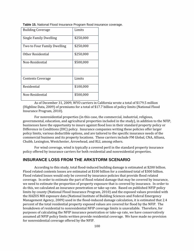
100

Table 15. National Flood Insurance Program flood insurance coverage.

Building Coverage Limits

Single Family Dwelling $250,000

Two to Four Family Dwelling $250,000

Other Residential $250,000

Non-Residential $500,000

Contents Coverage Limits

Residential $100,000

Non-Residential $500,000

As of December 31, 2009, WYO carriers in California wrote a total of $179.5 million (Highline Data, 2009) of premiums for a total of $17.7 billion of policy limits (National Flood Insurance Program, 2010).

For nonresidential properties (in this case, the commercial, industrial, religious, governmental, education, and agricultural properties included in the study), in addition to the NFIP, businesses have the opportunity to insure against flood loss in their standard property policy or Difference in Conditions (DIC) policy. Insurance companies writing these policies offer larger policy limits, various deductible options, and are tailored to the specific insurance needs of the commercial business and its property locations. These carriers include FM Global, CNA, Allianz, Chubb, Lexington, Westchester, Arrowhead, and RLI, among others.

For wind coverage, wind is typically a covered peril in the standard property insurance policy offered by insurance carriers for both residential and nonresidential properties.

INSURANCE LOSS FROM THE ARKSTORM SCENARIO

According to this study, total flood-induced building damage is estimated at $200 billion. Flood related contents losses are estimated at $100 billion for a combined total of $300 billion. Flood related losses would only be covered by insurance policies that provide flood related coverage. In order to estimate the part of flood related damage that may be covered by insurance, we need to estimate the proportion of property exposure that is covered by insurance. In order to do this, we calculated an insurance penetration or take-up rate. Based on published NFIP policy limits by county (National Flood Insurance Program, 2010) and the exposed values provided with the HAZUS MH exposure data (National Institute of Building Sciences and Federal Emergency Management Agency, 2009) used in the flood-induced damage calculation, it is estimated that 2.4 percent of the total residential property exposed values are covered for flood by the NFIP. The breakdown of residential to nonresidential NFIP coverage limits is unavailable. Therefore, for purposes of calculating the NFIP insurance penetration or take-up rate, we have conservatively assumed all NFIP policy limits written provide residential coverage. We have made no provision for nonresidential coverage offered by the NFIP.

101

Nonresidential flood coverage is provided by the NFIP standard commercial property policies or through Difference In Conditions policies, only if the flood risk is acceptable to the carrier. It is generally, expected that flood insurance will be purchased if the risk is acceptable and the insurance premium is reasonable. However, information about the actual take-up rate of nonresidential flood insurance coverage is not publicly available. For purposes of our analysis, we have assumed a range of take-up rates from 20 percent to 90 percent, varying by county. Our estimates vary by county in a similar proportion to the actual NFIP take-up rates with the highest coverage take-up found in the northern counties of Yuba, Sutter, and Colusa, just north of Sacramento.

For the calculation of an insured loss estimate, we have applied the penetration rates for residential and nonresidential flood insurance coverage to the flood damage estimates by county and line of business. For a flood damage estimate of $300 billion, we estimate the flood insurance loss to be in the range of $20 billion to $30 billion.

For wind insurance loss estimates, we must cite the “Efficient Proximate Cause” language, which comes into play in California insurance law. The efficient proximate cause applies to an “All Risk” insurance policy when a loss is caused by a combination of a covered peril and a specifically excluded peril. The loss is covered only if the covered peril was the efficient proximate cause. The loss is excluded if the excluded risk was the efficient proximate cause of loss. This is subject to interpretation and there have been many cases involving efficient proximate cause language (Johnson 1999), the subject and review of which is beyond the scope of this analysis. Flood damage exceeds the wind damage estimates in all counties in the ARkStorm scenario; therefore, flood damage was assumed to be the proximate cause of loss for all properties. Accordingly, only the flood insurance policy would respond for insurance coverage. Litigation and judicial rule may require wind policies to respond; however, this is not contemplated explicitly in our estimates.

For purposes of estimating the insurance loss, it is estimated that the flood policy will respond to offer coverage, to the extent a policy covering flood is in place. If no flood policy is in place, the wind policy would not respond because of the efficient proximate cause language.

Table 16 shows the estimated residential flood insurance loss, covered by the NFIP, and the estimated range of nonresidential flood insurance loss assuming a moderate and high level of insurance take-up.

Table 16. Insured loss estimate for different levels of insurance.

Residential Nonresidential* Total

NFIP only

Moderate

Insurance Take-up

High

Insurance Take-up

Moderate

Insurance Take-up

High

Insurance Take-up

$2.1 billion $20.1 billion $26.4 billion $22.2 billion $28.5 billion

*Commercial, Industrial, Religious, Governmental, Education, and Agricultural.

Computing the NFIP loss as a percentage of the insurance available, $2.1B per $17.7B, or 12 percent, is a reasonable damage ratio for the amount of insurance available. We are unable to perform the same calculation for nonresidential flood insurance because the amount of flood insurance written is unknown. However, we believe our estimates to be reasonable.

102

HISTORICAL PRECEDENT AND ECONOMIC RESILIENCY

California is best known for its earthquake and wildfire events. California is not generally known for its windstorm or flood events. In fact, since 1952, there have been 63 windstorm-related natural peril events and only 9 of these have involved some form of flooding. Interestingly, all the flood related events have occurred since 1995. The largest of these was an insured loss of just under $400 million in 2008 (Property Claims Service, written commun.). This report, however, provides the evidence that significant wind and flood events have the potential to occur.

The largest natural peril wind and flood insured loss event was Hurricane Katrina. Katrina was a Category 3 hurricane that made landfall on August 29, 2005. Katrina impacted the Louisiana and Mississippi coastlines with storm surge as high as 25 feet and contributed to the levee failure in New Orleans. For this reason, Katrina is thought of as two catastrophic events; the hurricane winds and the flood that ensued from the failure of the levee system. While total economic losses are not tracked, the estimated economic losses for Katrina exceeded $100 billion (Insurance Journal, 2005).

The insurance loss to Katrina is estimated at $41.1 billion (Insurance Information Institute, 2010) resulting from 1.7 million claims. This estimate does not include the total flood loss to the NFIP that is estimated at $16.1 billion from 167,000 claims (Federal Emergency Management Agency 2010b). Combined, the total insured loss is just under $60 billion.

Obviously, Katrina is not a direct comparison to the ARkStorm scenario but Katrina is the most relevant event in recent history. Katrina caused significant economic disruption in the New Orleans and Gulf coast region; disruption that remains today (2010); however, the impact to the U.S. economy was mitigated for a few reasons. First, the economic production capabilities as measured by the Gross State Product (GSP) of the Gulf region are lower than the national average. The GSP for Louisiana and Mississippi is $225 billion and $93 billion (Chantrill, 2010), respectively, compared to the national average of $292 billion. Next, the general population affected is small with 7.6 million people living in Louisiana and Mississippi or 2.1 percent of the U.S. population. Lastly, nearly 60 percent of the damages were insured that has provided the funds to allow people to rebuild, contributing to a faster recovery.

By contrast, for the ARkStorm scenario, the GSP of California is $1,870 billion or nearly 6 times that of Louisiana and Mississippi combined. The population of California is 38.1 million or 12.3 percent of the U.S. population. And it is, estimated that only 6 percent to 10 percent of the economic damages would be insured. Undoubtedly a repeat of the 1861-62 winter storm would have a significant impact not only on the California economy but on the U.S. economy as well.

RESEARCH NEEDS RELATED TO INSURANCE

These are the two most compelling research needs from our viewpoint:

1. Wind vs. Water: determining the primary cause of loss. Study ways to more quickly and efficiently

determine if wind or flood is the primary cause of loss. Efforts in this area will help reduce litigation

expense, reduce pressure on policyholders who may need to prove the cause of loss, and generally

create a more efficient claims handling process that will benefit insurers and policyholders alike.

2. NFIP reform. The current structure is not capable of handling the size of the loss potential today.

The primary rate needs to be reviewed for adequacy. Exploration into giving the NFIP some

authority to enforce appropriate construction to reduce risk or eliminate risk (by relocating

103

homes/communities). In our opinion, simply renewing the current process is not a sustainable

option.

Evacuation

During winter storms, weather forecasts may trigger evacuation of areas threatened by flooding or landslide susceptibility where precipitation is persistent. Despite the advantage of forewarning, existing social conditions in the evacuation areas can determine the success of an evacuation procedure. Our analysis of the ARkStorm scenario identifies some of the social conditions that could create evacuation challenges caused by flooding in the Inland Region and two additional delta counties: Contra Costa and Solano (Fig. 57). First we estimated the number of people in the flooded areas in the Inland Region and the two additional Delta counties, then we examined social variables that have complicated other massive U.S. evacuations and analyzed these variables in the ARkStorm flooded areas, and finally we applied the HAZUS-MH formula (Federal Emergency Management Agency, 2010b) for shelter requirements. Estimates of county populations in flooded areas were passed to the economic impact analysis. Future refinement of the evacuation analysis for regional planning purposes will expand the social variables and incorporate other factors that affect evacuation (for examples, elevation, traffic routes, shelters).

POPULATION LIVING IN FLOODED AREAS

We use the number of people living in the flood-hazard zones (designated as flooded in the ARkStorm scenario) as a proxy for evacuation numbers; we assume that these flooded areas are forecast with sufficient certainty and all occupants in flooded areas are evacuated. Typically, some people will refuse to evacuate (for example, because of pets), cannot evacuate (for example, because of disabilities), or try to hold out. Our estimate of people living in the flooded area indicates the order of magnitude of an ARkStorm scenario evacuation.

Review of contemporary newspaper coverage of previous storms with flood-related evacuations (James Carter, USGS, 2010, written commun.) revealed the following:

A total number of evacuees for the 1861-62 storms was not reported, but some accounts tell of 6-7 families sharing houses and 60 people residing in one room. Boats were “slapped together” in response to a scarcity of boats for evacuation.

In 1938, apparently tens of thousands of people were evacuated.

In 1969, helicopters evacuated sick and aged in isolated foothill areas.

In 1986, about 45,000 people were reported to have evacuated.

In 1997, the number of evacuees was on the order of 125,000 people.

The largest evacuation in the United States was in 2008 when over 3 million people were evacuated because of Hurricane Gustav (Global Risk Miyamoto, 2009). In 2005, the number of people older than 16 years old who evacuated from Hurricane Katrina was about 1.5 million according to U.S. Bureau of Labor Statistics (Groen and Polivka, 2008). Another important meteorological event was Hurricane Rita (2005). The emergency office in Harris County (Texas) envisioned an evacuation of 0.8-1 million people, but more than 2.5 million people fled from that county of 3 million citizens (Victoria Transport Policy Institute, 2006).

In order to obtain the number of people living in ARkStorm scenario flooded areas (Table 17; Figure 57), we used the ESRI 2009 projections of census-block population (table 17; fig. 57). (The projection is relative to the United States Census 2000.) For blocks that were partially flooded,

104

we calculated the proportion of the block population in the flooded area by using the National Land Cover Data (NLCD) of 2001. In partially flooded census block areas we calculated the area in high, medium, and low intensity of development and the proportion of developed land that was flooded. We assumed that the proportion of people living in flooded areas corresponds to the proportion of the developed area that is flooded. Our intent with this procedure is to avoid counting population that is concentrated outside of the flood zones. Despite the 8 years of difference between ESRI 2009 projections and the 2001 NLCD, we justify use of this procedure with the observation that most of the partially flooded blocks are located in rural areas, where population tends to be dispersed with no major changes in the distribution of growth in recent years. Thus, we estimate that 1.5 million people13 reside in the flooded areas of the ARkStorm scenario. Most of these people are concentrated in Sacramento and San Joaquin Counties, but Sutter County has the highest percentage (97 percent) of population living in a flooded area. These 1.5 million people represent about 20 percent of the population in the evacuation study area and even though we cannot affirm that all these people would need to evacuate in the ARkStorm scenario, previous events like Katrina and Gustav have demonstrated that evacuations around this size will require federal, regional, and state resources beyond the county capacity.

Figure 57. Estimates of number of people, per county, in areas flooded by the ARkStorm. Blue is fewer than 10,000 people, red is more than 400,000.

13 Using the proportion of area flooded as the proportion of the population in flooded areas raises

the total flooded population estimate by another 100,000 people.

105

Table 17. Estimates of county population living in flooded areas.

County Estimated 2009 population

People in flooded area

Population in flood area, in percent

Butte 221,957 33,467 15.08 Colusa 22,162 10,101 45.58 Contra Costa 1,063,951 85,445 8.03 Fresno 936,063 11,828 1.26 Glenn 29,084 3,424 11.77 Kern 830,563 22,020 2.65 Kings 155,116 9,632 6.21 Lassen 36,131 2,032 5.62 Madera 153,361 2,197 1.43 Merced 258,323 5,295 2.05 Modoc 9,662 1,197 12.39 Sacramento 1,432,760 527,885 36.84 San Joaquin 692,792 480,106 69.30 Shasta 183,135 22,043 12.04 Solano 426,258 76,486 17.94 Stanislaus 528,982 1,488 0.28 Sutter 97,353 94,024 96.58 Tehama 63,516 10,656 16.78 Tulare 440,882 1,755 0.40 Yolo 202,429 80,689 39.86 Yuba 75,240 56,262 74.78 Regional total 7,859,720 1,538,032 19.57 In addition to the aforementioned assumptions, we were unable to distinguish depth of flooding less than 3 feet. HAZUS methodology suggests that 1 foot is a threshold flood depth for the floatation of cars (Federal Emergency Management Agency, 2010b). On the other hand, other causes for evacuation besides flooding such as landslides, utility (water and power supply) outages and environmental conditions (for example, sewage back up) were not considered. Therefore, the number of people in the flooded areas likely overestimates flood induced evacuation while neglecting other causes for evacuation.

SOCIAL INDICATORS

According to studies of past evacuations (Cabinet Office Civil Contingencies Secretariat, 2006) and (Victoria Transport Policy Institute, 2006), social variables affect the ability of people (as individuals and groups) to evacuate. We analyzed some of those variables that are supported by census block data from the 2009 ESRI projections and the 2000 Census (for English speaking only). The social indicators were defined and justified as follows:

Population: Evacuations in more populated areas are more prone to problems associated with coordination of evacuees, traffic jams, mobilizing people with special needs, shelter availability and public transportation. The population indicator is measured as the number of people living in flooded areas of each census block. The population data are from the ESRI 2009 projection.

Age: A person’s ability to evacuate depends on physical self-sufficiency. Research has shown that the majority of deaths during emergencies occur in people older than 65. For example, 66 percent of the fatalities associated with Hurricane Katrina were older than 65 (Louisiana State

106

University, 2005). Also, in most cases when a large-scale evacuation is taking place, the senior population suffers the majority of the consequences. They get left behind by their caretakers, families, and even the authorities do not plan for their particular conditions or impediments (Cherry and others, 2009). For our analysis, the age indicator is the percentage of people over the age of 65 years in census blocks with flooding. The data for this statistic were taken from the ESRI 2009 projections.

Income: Per capita income is an indicator of mobility in an evacuation in two ways. First, income represents a capacity to afford services, for example, renting a car or staying in a hotel for a long period during an emergency. Second, people with higher incomes have better access to private transportation (own cars). Those with lower incomes tend to rely more on public transportation.

Our income indicator is per capita income by block. We obtained these data from the ESRI 2009 projections that are based on the block Per Capita Income of 2000.

Population density: The population density indicator highlights the more densely inhabited census blocks with flooding. Various studies such as Committee on Role of Public Transportation (2008) and American Highway Users Alliance (2006) reveal several factors that influence evacuation procedures and timing; population density is among these factors. Also, areas with high density tend to be located in urban areas where poverty is more concentrated. Consequently, people in high-density areas may need more assistance with evacuation.

Population density by definition is the census block population (ESRI 2009 population estimate) divided by the horizontal projected area of the block.

Diversity: The relationship between ethnic minority groups and response to an evacuation warning is a subject of research (Sorenson and Sorenson, 2006). In general, studies suggest that minority groups are less likely to evacuate, but Perry (1987) suggests that warning belief and personal risk are stronger determinants of evacuation compliance. However, he also notes that some minority groups perceive authority figures—particularly those from the government—differently from majority groups. In this case, a greater effort is required to accommodate more minority groups into an evacuation plan.

We use the Diversity Index (D.I.) formulated by ESRI that measures the diversity of races/ethnicities of people in a block. The D.I. ranges from 0 (no diversity, the population is comprised of a single ethnic group or race) to 100 (complete diversity, each member of the population is from a different ethnic group or race). By way of example, the U.S. Diversity Index of 61 means that there is a 61 percent probability that two people randomly chosen from the U.S. population belong to a different ethnic group or race (Environmental Systems Research Institute, Inc., 2009). Therefore, a block with a high D.I. has a variety and a balance of races/ethnicities. It is important to clarify that this indicator describes diversity and not the dominant presence of a specific ethnic group or race. The non-English speaking component of minority groups is isolated in the language indicator.

Language: Another major factor affecting evacuation compliance is language. Local authorities need to be aware of the languages spoken in their communities and potential language barriers. For example, the majority of people that died in the 1987 Saragossa Tornado in Texas were Hispanic and this outcome was attributed to a failure to provide a good translation of the warning into Spanish (Aguirre and others, 1991).

For the language indicator, we used English-speaking data from the Census 2000; we calculated the percentage of people in each block that did not speak English at all or were described to have “low English skills”.

107

Evacuation vulnerability index: In anticipation of summing the indicators to highlight census blocks that may be relatively more challenged by an evacuation, we normalized the data for each indicator by dividing each value by the maximum value for that indicator. Subsequently, for each block we added the normalized indicators and divided the result by 6 (number of indicators) to create an evacuation index that encompasses all 6 indicators. We mapped each indicator and evacuation index by using quantiles (table 18). The lowest (highest) values represent low (high) presence of that indicator. The evacuation index is calculated for the study region, but mapped for three zones (figs. 58 through 60) to display more detail.

Table 18. Scaling of social indicators for social vulnerability index.

Range/Percentiles Quantile/Value Description

No datum presence 0 No data

Lower 20th 1 Very low

21st to 40th 2 Low

41st to 60th 3 Medium

6 1st to 80th 4 High

81st to 100th 5 Very high

To capture the interaction between the social variables and severity of flooding, we scaled the flood variables of depth and duration by normalizing the data of each flood indicator (table 19), summing the results, and mapping the top 40 percent of the values to produced a spatial layer of more severe flooding—characterized by greater depth and longer duration. These areas with more severe flooding are shown in black shading (figure 56 through figure 59) to visualize the spatial relation between areas with a high evacuation index and areas with more severe flooding. Note that the flood variables are not incorporated into the evacuation index.

Table 19. Indicators for flood variables used in scaling of social vulnerability.

[<, less than]

Depth

(feet)

Duration

(days)

<3 <0.5

3 - 10 0.5-3

10 – 20 3-7

3-14

14-28

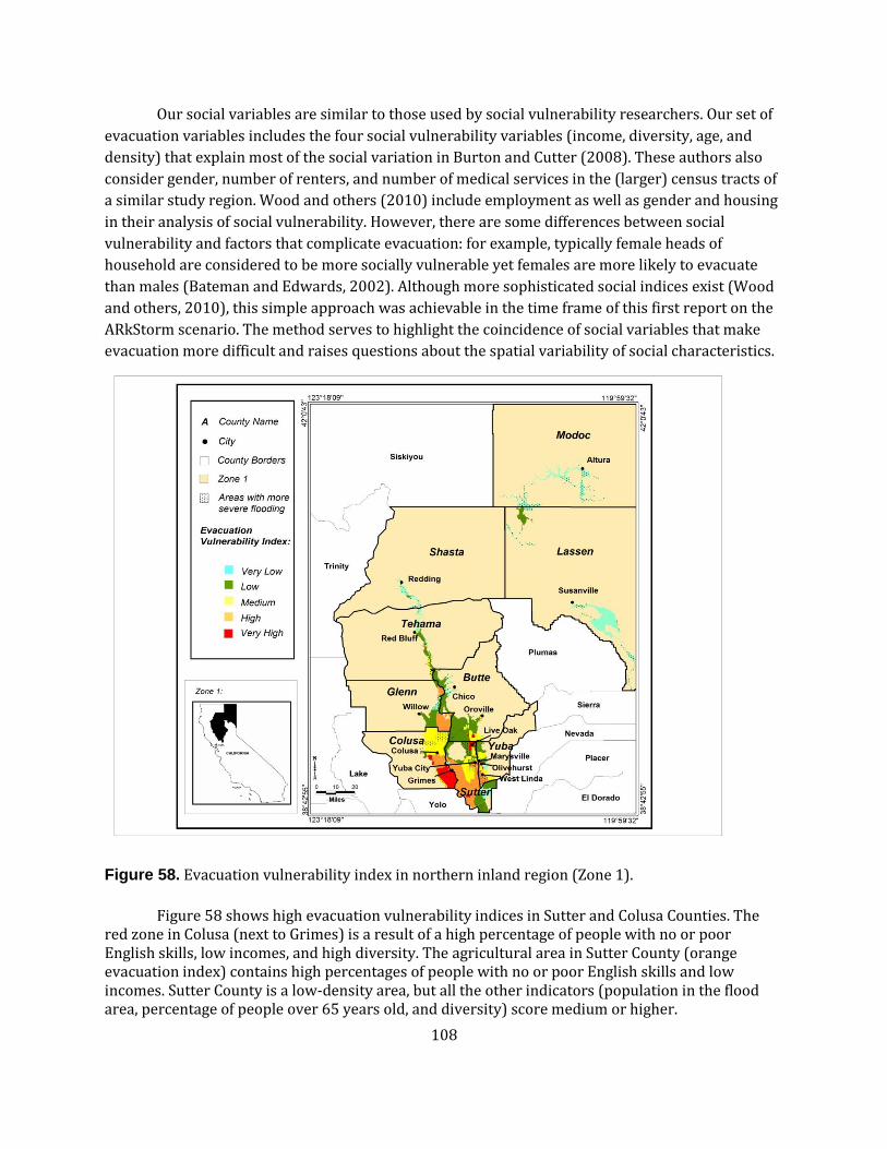
108

Our social variables are similar to those used by social vulnerability researchers. Our set of

evacuation variables includes the four social vulnerability variables (income, diversity, age, and

density) that explain most of the social variation in Burton and Cutter (2008). These authors also

consider gender, number of renters, and number of medical services in the (larger) census tracts of

a similar study region. Wood and others (2010) include employment as well as gender and housing

in their analysis of social vulnerability. However, there are some differences between social

vulnerability and factors that complicate evacuation: for example, typically female heads of

household are considered to be more socially vulnerable yet females are more likely to evacuate

than males (Bateman and Edwards, 2002). Although more sophisticated social indices exist (Wood

and others, 2010), this simple approach was achievable in the time frame of this first report on the

ARkStorm scenario. The method serves to highlight the coincidence of social variables that make

evacuation more difficult and raises questions about the spatial variability of social characteristics.

Figure 58. Evacuation vulnerability index in northern inland region (Zone 1).

Figure 58 shows high evacuation vulnerability indices in Sutter and Colusa Counties. The red zone in Colusa (next to Grimes) is a result of a high percentage of people with no or poor English skills, low incomes, and high diversity. The agricultural area in Sutter County (orange evacuation index) contains high percentages of people with no or poor English skills and low incomes. Sutter County is a low-density area, but all the other indicators (population in the flood area, percentage of people over 65 years old, and diversity) score medium or higher.

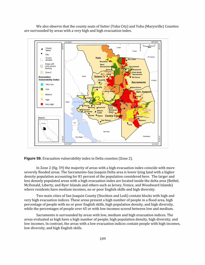
109

We also observe that the county seats of Sutter (Yuba City) and Yuba (Marysville) Counties are surrounded by areas with a very high and high evacuation index.

Figure 59. Evacuation vulnerability index in Delta counties (Zone 2).

In Zone 2 (fig. 59) the majority of areas with a high evacuation index coincide with more severely flooded areas. The Sacramento-San Joaquin Delta area is lower lying land with a higher density population accounting for 81 percent of the population considered here. The larger and less densely populated areas with a high evacuation index are located inside the delta area (Bethel, McDonald, Liberty, and Ryer Islands and others such as Jersey, Venice, and Woodward Islands) where residents have medium incomes, no or poor English skills and high diversity.

Two main cities of San Joaquin County (Stockton and Lodi) contain blocks with high and very high evacuation indices. These areas present a high number of people in a flood area, high percentage of people with no or poor English skills, high population density, and high diversity, while the percentages of people over 65 or with low incomes scored between low and medium.

Sacramento is surrounded by areas with low, medium and high evacuation indices. The areas evaluated as high have a high number of people, high population density, high diversity, and low incomes. In contrast, the areas with a low evacuation indices contain people with high incomes, low diversity, and high English skills.

110

Figure 60. Evacuation vulnerability index in southern inland region (Zone 3).

Zone 3 (fig. 60) exhibits the smallest amount of area with severe flooding. These areas are northwest of the zone. We identify two main areas of high evacuation indices. The first area is next to Firebaugh City. Blocks in this area contains a high percentage of people with poor English skills, high diversity, and low income while the number of people, and percentage of people over 65 years old scored lower (values between 2-3). Density score was very low (1). Kettleman City blocks contain a high percentage of people with no or poor English skills and low income while the number of people, percentage over 65 years old, and diversity fluctuated between 1and 3. Again, density scored the lowest possible value of 1.

111

Figure 61. Percentage of people in top two quantiles of the evacuation index relative to the total population (2009) by county.

By way of summary, Figure 61 displays the percentage of people living in the flooded blocks with high and very high evacuation indices for each county. Except for Contra Costa and Solano Counties, the counties with the larger populations in flooded areas (table 17) also have a higher percentage of people living in blocks with high evacuation vulnerability according to our index. Consequently, both San Joaquin and Sacramento Counties have high absolute (over 300,000 people in both counties) and relative numbers of people residing in blocks with high evacuation indices. However, the less populated Colusa County also has a high percentage of people in the top two quantiles of the evacuation index. It is no surprise that Sutter County has the highest percentage of population in blocks, with high and very high evacuation indices, because 97 percent of the county population is in the ARkStorm flooded area.

SHELTER REQUIREMENTS

We estimated the number of people who may need temporary shelter after ARkStorm by using methods in the HAZUS®MH MR4 technical manual (National Institute of Building Sciences and Federal Emergency Management Agency, 2010). This formula takes into account the following factors:

Low income families that lack the means to find other shelter on their own.

4.2%

29.6%

2.3%

1.5%

9.7%

2.3%

9.6%

1.3%

2.1%

27.5%

48.4%

5.8%

0.3%

59.4%

2.1%

0.5%

34.4%

48.3%

0.0% 10.0% 20.0% 30.0% 40.0% 50.0% 60.0% 70.0%

Butte

Colusa

Contra Costa

Fresno

Glenn

Kern

Kings

Madera

Merced

Sacramento

San Joaquin

Solano

Stanislauss

Sutter

Tehama

Tulare

Yolo

Yuba

Percentage

Co

un

tie

s

112

Young and elderly families that may have the means of finding temporary shelter on their own, but prefer to use publicly provided shelters.

The formula to calculate the number of people with shelter needs is the following:

5 3

1 1

k m

k m

STP akm DP HI HA

(4)

where

STP= number of people using established shelters

DP= Displaced population

αkm= Constant for income and age class

HIk= Percentage of population in the kth household income class

HAm= Percentage of population in the mth age class

The 2009 income data were provided by the ESRI projections. The age data are from the 2000 census because the 2009 ESRI projection age data were not available.

Table 20. Estimates, per county, of numbers of people in flood area.

Includes number and percentage of those needing short-term shelter.

County Estimated total people in flood area

Estimated number of people in need of short-term shelter

Percentage

Butte 33,467 4,767 14.24 Colusa 10,101 1,298 12.85 Contra Costa 85,445 10,227 11.97 Fresno 11,828 1,942 16.42 Glenn 3,424 257 7.51 Kerns 22,020 2,787 12.66 Kings 9,632 561 5.82 Lassen 2,032 257 12.65 Madera 2,197 468 21.30 Merced 5,295 740 13.98 Modoc 1,197 147 12.28 Sacramento 527,885 76,073 14.41 San Joaquin 480,106 76,118 15.85 Shasta 22,043 3,022 13.71 Solano 76,486 9,899 12.94 Stanislaus 1,488 272 18.28 Sutter 94,024 10,399 11.06 Tehama 10,656 1,658 15.56 Tulare 1,755 418 23.82 Yolo 80,689 11,502 14.25 Yuba 56,262 7,509 13.35 Total 1,538,032 220,321 14.32

113

The results in table 20 suggest that 8 percent (125,022) of the population in the Inland Region and Contra Costa and Solano Counties may need shelter in the short-term. San Joaquin and Sacramento County residents are in greater need of short-term shelters for about 100,000 people, representing 84 percent of all shelter needs. The concentration is caused by the combination of two main features of these counties: a large number of people residing in the flooded area (table 17) and a relatively high percentage of lower income population. (As another point of reference, according to the 2000 Census, 18 percent of San Joaquin and 14 percent of Sacramento County residents were living below the poverty line.)

RESEARCH NEEDS RELATED TO EVACUATION

For census blocks with partially flooded areas, further refinement of flooded population estimates can be accomplished by identifying important features of the residential population. For example, Solano County has a high number of people living in houseboats. These people may not need to be evacuated. Also additional variables like car ownership and household gender could be considered to further inform the spatial variability of evacuation issues. Another key variable affecting people’s ability to evacuate is the number of people with disabilities and health issues. The Flood Emergency Action Team (FEAT) final report (California Department of Water Resources, 1997) concluded that warnings and shelters were not accommodating of people with disabilities. The location of people with disabilities and health issues is not readily available and is challenging to keep current. The Sacramento County evacuation plan (Sacramento County, California, 2008) describes various strategies for locating, alerting, and warning this vulnerable population. Elsewhere, the Florida ADA Hurricane and Disaster Center has partnered with the Center for Independent Living of Southwest Florida and emergency preparedness officials to track this information in four Florida counties (Cahalan and Renne, 2007).

An additional consideration is public transportation as an asset for massive evacuation. Issues around transportation are well illustrated by Hurricanes Katrina and Rita. -“If Katrina exposed what happened when many people have no cars to evacuate; Rita seemed to show the other side of the coin”- (Victoria Transport Policy Institute, 2006). During Katrina, the demand for transportation was massive, but the city was not ready for such demand. The lack of planning and concrete strategies for people with no private transportation provoked the public to take over infrastructures that were not designated to become shelters. Also, many people with special needs for transportation were left behind, increasing the number of fatalities. In contrast, during Hurricane Rita, emergency managers in Texas expected people in coastal areas who owned boats to take the boats with them by trailer and cause additional congestions on the roads. However, they had not anticipated families using all their cars to evacuate (rather than take one car per family) and in some cases residents took trailers and horse trailers as well. This evacuation led not only to very heavy congestion on the road but also to a shortage of gas (Cabinet Office Civil Contingencies Secretariat, 2006). Public transportation is an asset and is key to a successful evacuation, but the challenges include overcoming the stigma of public transportation, improving efficiency, identifying rally points, and educating residents (Victoria Transport Policy Institute, 2006). Overall, evacuation planning needs to consider a range of public services for the evacuees (such as gas stations, supermarkets, health care, public buses) and the management and retention of staff for those services.

The evacuation analysis can be enhanced with considerations of public infrastructure, location of shelters and dams, and options for public transportation.

114

Elevation data can be used to identify suitable shelter sites. Integration of various spatial information will be useful for regional evacuation planning. One example of spatially integrated information at the local level is the evacuation mapping designed by Baldwin (2010) for San Joaquin County.

Finally, a concern of CalEMA is the level of complacency about evacuation in California (D. Owens, CalEMA, 2010, personal commun.). In contrast to the Gulf States, the residents of California are not routinely faced with flooding and evacuation warnings and orders. Tendencies to ignore official warnings and wait until the last minute to evacuate will put more people at risk. Changing passive perceptions toward flooding evacuations is a challenge for emergency managers because people’s risk attitudes and beliefs is what makes evacuation a reality.

Business Interruption Costs

INTRODUCTION

This section summarizes business interruption (BI) impacts of the ARkStorm Scenario. These impacts stem from a combination of damage to buildings, agricultural lands, and several types of infrastructure. Our BI estimates include not only direct impacts at the site of the damage but also indirect BI stemming from interdependencies among and between businesses and households throughout the economy.

Our direct BI estimates are based on calculations of loss of building function, loss of productivity on agricultural land, reduction of lifeline services from damaged infrastructure, and a reduction in the labor force because of evacuation. These estimates are translated into decreases in the capital stock or direct declines in output, as appropriate, into 100 sectors of the economy.

Our indirect BI losses are based on the application of a dynamic computable general equilibrium (CGE) model of the California economy. CGE is a state of the art economic tool that is based on the behavioral response of representative producers and consumers to market price signals within the limits of available capital, labor, and natural resources (Shoven and Whalley, 1992). CGE captures both technical interdependence between sectors in terms of input linkages and also market actions and interactions through prices. The dynamic feature links the 6-month time periods in the model (appendix B). CGE models are increasingly being used in disaster context (Rose and Liao, 2005; Rose and others, 2009; Dixon and others, 2010). This study further advances the methodology for application to disasters.

HAZARD LOSS ESTIMATION

BASIC CONSIDERATIONS

For many years, hazard loss estimation was dominated by engineers, and accordingly the focus was on property damage to structures. Other types of impacts (whether economic, sociological, psychological) were combined in a grab bag category termed "indirect" or "secondary" losses. By the mid-1990s, there was a growing appreciation of the role of business interruption (BI) losses, which refer to the reduction in the flow of goods and services produced by property (capital stock). This stock/flow

115

distinction is a basic concept in economics and, in fact, flow measures, such as Gross National Product (GNP), have long held a dominant position.

Direct and indirect versions of both categories of losses are prevalent. Direct property damage relates to the effects of flooding, winds, and landslides; while collateral, or indirect, property damage is exemplified by toxic releases from HAZMAT facilities (those in the EPA facility registry system) damaged by flood debris. Such indirect property damages have been identified under environmental and health issues in this report, but we have not been able to evaluate the economic impacts of them. Direct BI refers to the immediate reduction or cessation of economic production in a damaged factory or in a factory cut off from at least one utility lifeline. Indirect BI stems from the interdependencies of the economy in the form of “multiplier" effects associated with the supply chain or customer chain of the directly affected business or through the general equilibrium effects of market interactions. Rose (2004a) explains these concepts and Rose and others (2009, National Research Council (2005, Multihazard Mitigation Council (2005a, 2005b), and European Union (2003), provide examples of the application.

An important consideration is that nearly all direct property and ancillary (or indirect) property damage takes place during the time span of the winter storm. An exception is damage from deep seated landslides: while some landslides, triggered by the heavy rainfall season including the ARkStorm, will begin to move during or shortly after the storm they may continue to move for months or years. Furthermore, other deep-seated landslides may not begin to move until weeks or months following the storm. BI, being a flow variable, manifests over a longer time period than storm related damage. BI begins when the damages from flooding, wind, and landslides occurs and continues until the built environment is repaired and reconstructed to some desired or feasible level (not necessarily predisaster status) and a healthy business environment is restored. As such, BI is complicated because it is highly influenced by the choices of private and public decision makers about the pattern of recovery, including repair and reconstruction. As in the ShakeOut scenario (Rose and others, written commun.; Jones and others, 2008,), the aggregate magnitude of BI can rival that of property damage. Also, technological progress implies that, over the long run, reconstruction investment that replaces old, less efficient capital with new, more efficient capital may generate a temporary increase in the aggregate productivity of capital and pay positive dividends offsetting some loses in the long-run.

More recently, the loss estimation framework has been expanded in two ways, and the term economic consequence analysis is being used to distinguish this breadth (Rose, 2009). First is the incorporation of the loss reduction strategy of resilience, in both static and dynamic forms. We define static economic resilience as the ability of an entity or system to maintain function (continue producing) when shocked by the types of disruptions accounted for in this scenario (Rose, 2009; 2004b;). Static economic resilience is thus aligned with the fundamental economic problem of efficient resource allocation, which is exacerbated in the context of disasters. This aspect is interpreted as static because it can be attained without repair and reconstruction activities, which affect not only the current level of economic activity but also its future time path. Another key feature of static economic resilience is that it is primarily a demand-side phenomenon involving users of inputs (customers) rather than producers (suppliers). This is in contrast to supply-side considerations, which definitely require the repair or reconstruction of critical inputs. A more general definition of dynamic resilience is the speed at which an entity or system recovers from a severe shock to achieve a desired state. This also subsumes the concept of

116

mathematical or system stability, as it implies the tendency of the system to “bounce back”. This version of resilience is relatively more complex, because it involves a long-term investment problem associated with repair and reconstruction. Production may be affected by building damages, reduced lifeline services, and absent employees.

The second major consideration is extended linkages. One type is systems linkages, such as cascading infrastructure failures. Another is behavioral linkages, which refer to considerations like the effect of recent disasters on risk attitudes (Burns and Slovic, 2007). A good example is the fact that 85 percent of the BI loss following 9/11 stemmed from the nearly 2-year decline in air travel and related tourism because of heightened fear of flying (Rose and others, 2009). Note this category also has associated indirect effects. Thus it can increase BI losses by one or two orders of magnitude. In the following analysis, we take these various considerations into account to the extent possible within project limitations. Throughout our modeling, we carefully distinguish stock from flow effects and direct from indirect losses. We factored in BI associated with interdependent infrastructure failures. We included some major sources of resilience in the aftermath of disasters relating to static resilience strategies of substitution responses to price signals, the ability to recapture lost production through overtime or extra shifts, and the fact that not all aspects of economic activity require infrastructure inputs. However, we were not able to factor in behavioral linkages.

CONDUITS OF ECONOMIC SHOCKS

We analyze the following conduits of shocks to the economic system stemming from damages to the built environment (Actual damage is not necessary in all cases to cause economic loss. Evacuation prior to disaster can cause even greater BI losses than a small version of the event. Also, some buildings can be closed for business because of proximity to damaged buildings. Some infrastructure services may be shut down as a precautionary measure as well.):

Direct building and content damage from flood

Direct building damage from wind

Direct damage to crops, fruit and nut trees, and agricultural lands

Direct lifeline service outages for:

Electric power systems

Water systems

Wastewater treatment systems

Highway networks

Telecommunication systems

Evacuation

An important additional consideration is the need to adjust for double-counting of the channels of losses. That is, a factory may suffer from a flooded first floor and loss of electricity simultaneously, either one being enough to cause it to shut down business operations. Our analysis does adjust for possible double-counting.

117

Finally, we note that our results could be presented in terms of several economic impact indicators. We first present them in terms of property damage (loss of asset values). We also calculate the results in terms of two types of flow variables relating to BI. The first is value added, a net measure that corresponds only to the cost of primary factors of production (labor, capital, and natural resources, and excludes the cost of intermediate, or processed goods). The second is Gross Domestic Product (GDP), which differs only slightly from value added by including some taxes. GDP at the state level is sometimes referred to as Gross State Product (GSP. The term "Gross" here refers to the fact that depreciation (wear-and-tear or obsolescence of fixed capital assets) is included, although intermediate goods are not. )

THE DYNAMIC COMPUTABLE GENERAL EQUILIBRIUM MODEL

A CGE model is a stylized computational representation of the circular flow of the economy (Shoven and Whalley, 1992). CGE solves for the set of commodity and factor prices and the set of activity levels of outputs from firms and household incomes that equalize supply and demand across all markets in the economy (Sue Wing, Boston Univ., written commun., 2009). The model developed for this study divides the California economy into 100 industry sectors, each of which is modeled as representative firm characterized by a constant elasticity of substitution (CES) technology to produce a single good or service. Households are modeled as a representative agent with CES preferences and a constant marginal propensity to save and invest out of income. The government also is represented in a simplified fashion. Its role in the circular flow of the economy is passive: collecting taxes from industries and passing some of the resulting revenue to the households as a lump-sum transfer, in addition to purchasing commodities to create a composite government good which is consumed by the households. Three factors of production are represented in the model: labor—which responds to changes in the wage rate, and two types of capital—intersectorally mobile, and sector-specific varieties of capital. These factors are owned by the representative agent and rented to the firms in exchange for factor income. California is modeled as an open economy that engages in trade with the rest of the U.S. and the rest of the world by using the Armington specification (imports from other states and the rest of the world are imperfect substitutes for goods produced in the state).

The static component of the model computes the prices and quantities of goods and factors that equalize supply and demand in all markets in the economy, subject to constraints on the external balance of payments. This equilibrium submodel is embedded in a dynamic process, which on a 6-month time-step specifies exogenous improvements in firms’ productivity and updates the capital endowments of the economy based on investment-driven accumulation of the stocks of capital. The impacts of a severe storm are modeled as exogenous shocks to the productivity of industries, and contemporaneous destruction of capital stock, with concomitant reductions in the California economy’s endowments of malleable and sector-specific capital input.

The model is formulated as a mixed complementarity problem using the MPSGE subsystem for the General Algebraic Modeling System (GAMS) software (Rutherford, 1999; Brooke and others, 1998) and is solved by using the PATH solver (Ferris and others, 2000). A more detailed and technical presentation of the model is presented in appendix B. The model is calibrated by using an IMPLAN social accounting matrix for the state of California for the year 2007 (Minnesota IMPLAN Group, 2006 in conjunction with values of the

118

elasticities of substitution and transformation drawn from Rose and others, (2009) and Rose and Liao (2005). The latter parameters are summarized in appendix B, which also provides a list of the sectoring scheme.

We model the consequence of the imposition of the storm’s shock as an array of initial declines in sector outputs, which induce intra- and intersectoral substitution adjustments by producers and consumers, as well as changes in the prices of commodities and factors. The result is a new equilibrium with reduced aggregate expenditure and investment, which generates contemporaneous losses of consumer welfare (relative to the baseline solution of the model), and slower growth of the capital stock that adversely affect the economy’s capital endowment and productive capacity in subsequent periods. The latter, dynamic impact of the initial capital stock destruction is an important source of hysteresis in the losses caused by a storm. Symmetrically, the principal channel through which repair and reconstruction investments dampen the persistence of losses is the output- and income-enhancing effect of restoring business productive capacity.

METHODOLOGICAL DETAILS FOR INDIVIDUAL LOSS CATEGORIES

In addition to the IMPLAN social accounting matrix, other data are critical for evaluating economic impacts and resilience associated with disasters. These data include inventory data on the built environment (commercial and industrial property, residences, infrastructure) and on the natural environment. Also needed is a set of damage functions that relate changes in underlying conditions to property damage and loss of function. One such source is Hazards United States-Multi-Hazard (HAZUS-MH) System (Federal Emergency Management Agency, 2008a). HAZUS-MH is a large expert system that contains detailed data on the built environment at the small area level, a set of damage functions, and a GIS capability. Physical damage and business interruption are translated into direct dollar values of building repair costs and business downtime costs, respectively.

Estimation of the conduits of business interruption was as follows:

1. Flood damaged buildings. The flooded building damage estimates provided to us were calculated by using HAZUS-MH equations. (The HAZUS-MH building inventory was extracted from the HAZUS-MH software because of the size of the problem) The flow of goods and services emanating from damages to this productive capital stock (essentially equivalent to BI losses) is direct “output loss”, where output refers to "gross output," equivalent to gross sales revenue. We followed the procedures in Chapter 14 of the HAZUS-MH flood technical manual (Federal Emergency Management Agency, 2010b) to calculate: (1) output losses for nonresidential occupancy classes and nursing homes and (2) rental and owner occupied losses for the remaining residential occupancy classes. We included the HAZUS-MH flooded building downtime add-ons of dry out and cleanup; inspection, permitting and ordinance approval; contractor availability; and hazmat delay. We used HAZUS-MH equations to calculate relocation costs. Flooded buildings and moderately damaged, severely damaged, and destroyed buildings will take longer to restore than the lifeline services, which are mostly recovered within two months. After two months, residual power restoration continues only in Mono, Inyo, and Tulare Counties.

2. Wind damaged buildings. Likewise, the building wind damages were provided to us by Keith Porter. We used the procedures in Chapter 7 of the HAZUS-MH Hurricane Technical Manual (Federal Emergency Management Agency, 2010d) to calculate output, owner-occupied dwelling, and rental losses.

119

3. Damages to agricultural commodities. An adaptation of the methodology developed for the Delta Risk Management Strategy (DRMS) (California Department of Water Resources, 2008) was used to estimate agricultural damages. Field repair costs were calculated for annual and perennial crops and livestock. In addition, forgone income was calculated for flooded annual crops; perennial crops flooded for 2 weeks or more incurred crop replacement costs and forgone income for up to 5 years; and the replacement value of livestock (dairies, feedlots, poultry) at risk was estimated in areas with at least 6 feet of flood depth.

4. Electric Power. One feature of the computations for most of the infrastructure categories involved is the timing of the disruptions. (For buildings this feature was internal to the HAZUS-MH computations.) The percentage of customers affected by the outages is not constant but decrease over time as services are restored. Like buildings, wind and flood damages to infrastructure were considered. The more dominant cause of damage was identified for each infrastructure in each county. Service reduction and restoration curves were based on panel discussions and expert opinion. Each infrastructure BI impact was simulated separately.

The power restoration pattern (percentage of power services recovered in individual restoration periods) differed by county and ranged from 0.2 percent to 69 percent customers initially out of service with most restored within a month except for a couple of outlier counties needing 6 months to fully restore power to customer base. The power outages were localized to county because generation capacity that is located “high and dry” was not considered to be a limiting factor. Each county restoration curve was transformed into quarterly power shortages for each occupancy class by (1) integrating under the inverse of each county restoration curve to estimate percentage of county customers not served during each quarter, (2) weighting this percentage by the proportion of occupancy class square footage in the county and (3) summing up weighted county power shortages for each occupancy class.

5. Water. The estimation of BI losses stemming from disruption of the water system is similar to that of the power system except that flooding was the only cause of damage. Consequently, 42 counties were not affected by water supply disruptions. The remaining counties have disrupted water services to 10-60 percent% of customers with service restored within three months.

6. Wastewater. The estimation of BI losses stemming from disruption of the wastewater system is similar to that of the water system. Forty-one counties were not affected by wastewater treatment disruptions. The remaining counties presented disrupted wastewater services to 17-100 percent of customers with service restored within a month.

7. Telecommunications. The estimation of BI losses stemming from disruption of the telecommunications system is similar to that of the power system. All counties experience reduced telecommunication services affecting 2 to 25 percent of customers for up to 7 days.

8. Truck Transportation. The truck traffic economic impact analysis was conducted outside of the CGE model and is described in a separate section. We obtained technical support from various University of Southern California-affiliated independent consultants coordinated by Hanh Le Griffin of TTW, Inc. Their transportation model analyzes the effects of reduced highway capacities on the regional and national movement

120

of goods and services by estimating changes in truck distance, travel time, and associated costs and the impacts of increased shipping prices on major economic sectors.

9. Evacuation. We were provided with county estimates of population in the ARkStorm flooded areas (based on GIS analysis by using ESRI 2009 population projections). About 1.5 million people reside in the ARkStorm flooded area of the Inland region and Delta counties. We assumed that the effective impact from evacuation extended for the duration of the flooding. IMPLAN county employment data (Minnesota IMPLAN Group, 2006 was used to allocate the evacuated population to sectors, that is, we assumed that the distribution of employment among evacuated residents is the same as the distribution of employment in the county.

RESILIENCE

For the most part this study only addresses aspects of static resilience because we received one restoration time path for each BI conduit and because dynamic resilience, especially for infrastructure, is so strongly dependent on a series of public and private decisions regarding the timing of repair and reconstruction, which are complex and uncertain and hence highly variable. Moreover, only a limited number of static resilience options were incorporated, albeit they are by far the ones that have been found to have the greatest potential for reducing BI losses (Rose and others, 2009).

The primary source of static resilience is “production rescheduling,” or the ability of firms to work overtime or extra shifts after they have repaired or replaced the necessary plant and equipment and their employees and critical inputs become available once more such that “loss of function” has been overcome. This is rather straightforward for the case of flood and wind damaged buildings. For infrastructure, it is more complicated. Just because electricity service has been restored does not mean that businesses can immediately turn on the assembly line; they must repair the necessary plant and equipment first (though this need not be 100 percent restoration to be fully operational). HAZUS-MH includes an adjustment for this consideration, referred to as the “Building Service Interruption Time Multiplier” for earthquakes and wind (hurricanes), but an adjustment has not yet been developed for the buildings damaged by flooding. Production rescheduling is incorporated in HAZUS-MH through the inclusion of production “recapture factors” (RFs), scaling parameters that represent the percentage of direct gross output losses that can be recovered at a later date. The original HAZUS-MH RFs range from 0.30 to 0.99. Manufacturing enterprises that produce nonperishable commodities are at the high end, while sectors producing perishables ( agricultural) or nonessential services (entertainment) are at the lower end of the scale. These RFs are subject to the caveat that they are applicable only for three months with no effect thereafter. This is meant to reflect the fact that customers and suppliers will grow impatient as their orders go unfilled. Accordingly, we adjusted the HAZUS-MH RFs downward by a linear decay rate of 25 percent for every 3-month period during the first year, so that recapture becomes zero by the second year. In our view, this reflects a more realistic situation in which customers become increasingly impatient over time, canceling larger numbers of orders as delays mount.

The second type of resilience modeled was infrastructure “importance.” The term stems from Applied Technology Council-25 (1991), which convened a panel of experts to advance hazard loss estimation. One of the contributions was to identify the percentage of a sector’s business operations that does not depend on a specific category of infrastructure.

121

Thus, even if a lifeline outage occurs, a part of the sector can keep operating. Examples are headquarters offices being less dependent than production lines in general, and some sectors being less dependent than others on lifeline services (the relatively low dependence of agriculture on the delivery of electricity and natural gas through the existing transmission and distribution infrastructure). Typically, the operation of industrial and commercial establishments is dependent on the availability of electricity, water, and natural gas, in that order. Like production rescheduling, this type of resilience also dissipates over time, though in a less dramatic manner. For example, if activities of headquarters or maintenance facilities are disrupted, other business functions may still be able to continue, but eventually inoperable headquarters and maintenance activities will disable the other functions of the enterprise. Unfortunately, no data were available to make adjustments that reflect this additional complication.

Rose (2009, 2004b) has emphasized that resilience has several key dimensions. One is that resilience can take place at the micro (individual business or household), meso (sector), and macro (economy-wide) levels. Another is the distinction between inherent and adaptive resilience. The former refers to features that exist in the economy under normal circumstances. The latter refer to adjustments that arise out of the ingenuity of the situation. A good example of the former is a dual-fired electric generation boiler, so that it is possible to substitute fuel oil for natural gas. An example of adaptive substitution would be to further modify the boiler after the flood to be able to burn waste products.

The market system is a major source of resilience. Price increases signal that resources have become more scarce, and, thereby, have a higher value, and that we should reallocate inputs accordingly. Note, all price increases do not represent gouging, and our CGE model is able to estimate what increases are warranted on the basis of economic efficiency. The CGE model also incorporates substitution possibilities as part of the production function of individual businesses.

Because of a lack of other information, we have often employed scalar or linear relationships to characterize resilience. At the same time, we must acknowledge that there is likely to be a threshold at which even resilience is eroded, beyond which the economic system will be overwhelmed and rendered much less able to return to pre-disaster equilibrium.

ADJUSTMENT FOR MULTIPLE SOURCES OF BUSINESS INTERRUPTION

Many businesses and households will suffer disruptions from many sources. They may simultaneously incur building damage and loss of one or more lifeline services. Thus, each of our estimates when totaled may double-count some impacts—the same business establishment cannot be shut down more than once in any given period. We adjusted for these multiple causes of failure (table 21), using the following procedures:

1. We identify uncorrelated conduits of economic shocks. Building damage because of wind occurs in higher elevation areas and building damage because of flood occurs in lower elevation areas. Therefore, we assume that the impacts from flood and wind building damage are additive (no double-counting). The economic impacts from crop and livestock damages also are treated as additive because they are calculated independently of building damages.

122

2. We identified additional superfluous lifeline impacts. We observed that the times to restore flood damaged buildings and buildings with moderate wind damage or greater exceed the time to restore power, water, wastewater, and telecommunication services. Therefore, if a flooded building or moderately or severely wind damaged or destroyed building is subjected to lifeline outages, the lifeline service will most likely be standing by to provide service once the building repairs are completed. Therefore, we accounted for the additional economic impacts from lifeline service outages affecting operations in buildings that have no downtime from flooding or are not moderately or severely damaged or destroyed by wind. We estimated these additional economic impacts from lifeline service outages by the following means:

a. First, we compared the percentage of building square footage with longer downtimes than lifeline service restoration times with the percentage of customers affected by each lifeline service outage. Across the building occupancy classes, about 21-36 percent of building square footage have downtimes exceeding lifeline service restoration times. The high technology HAZUS-MH occupancy class (IND 5) is an outlier with 70 percent of building square footage with downtimes exceeding lifeline service restoration times. On average, 25 percent of building square footage have downtimes longer than lifeline service restoration times. Weighted averages of initial lifeline service outages suggest that 12 percent, 16 percent, 21 percent, and 24 percent of building square footage is subjected to water, telecommunications, power, and wastewater service outages, respectively. Therefore, it is possible that all or most lifeline service outages affect buildings with downtimes longer than lifeline service restoration.

b. Second, at the other extreme, we considered the case of equal distribution of lifeline service outages across building square footage such that building damages and lifeline outages are essentially treated as independent of each other. Weighting initial county lifeline service outages with county building square footage, suggests that, on average, 60 percent of the water and wastewater outages could pertain to buildings with downtimes less than lifeline service restoration. Similarly, on average, 75 percent of the power and telecommunications outages could pertain to buildings with downtimes less than lifeline service restoration. The lower percentage for water and wastewater is not surprising given that flooded components of the water and wastewater systems yielded a greater percentage of service outages in those counties with more building flood damage. Thus, additional impacts from lifeline service outages after building damage could be in the range of 0-60 percent of water and wastewater service economic impacts and 0-75 percent of power and telecommunication service economic impacts.

c. Third, we selected a percentage within the above ranges by considering the likely spatial correlation between damaged buildings and lifeline service disruptions. Further data and GIS analysis is needed to assess the distribution of flooded building square footage relative to water and wastewater service areas. In the absence of this information, we surmise that these lifeline service reductions disproportionately affect flooded buildings because flooding is the cause of water and wastewater infrastructure damages. Within the possible range of 0-60 percent of additional economic impacts from water and wastewater outages, we assumed 10 percent of water and wastewater economic impacts qualified as additional. Power service outages, for the northern region at least, were calculated with double counting in

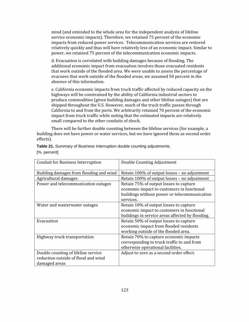
123

mind (and extended to the whole area for the independent analysis of lifeline service economic impacts). Therefore, we retained 75 percent of the economic impacts from reduced power services. Telecommunication services are restored relatively quickly and thus will have relatively less of an economic impact. Similar to power, we retained 75 percent of the telecommunication economic impacts.

d. Evacuation is correlated with building damages because of flooding. The additional economic impact from evacuation involves those evacuated residents that work outside of the flooded area. We were unable to assess the percentage of evacuees that work outside of the flooded areas; we assumed 50 percent in the absence of this information.

e. California economic impacts from truck traffic affected by reduced capacity on the highways will be constrained by the ability of California industrial sectors to produce commodities (given building damages and other lifeline outages) that are shipped throughout the U.S. However, much of the truck traffic passes through California to and from the ports. We arbitrarily retained 70 percent of the economic impact from truck traffic while noting that the estimated impacts are relatively small compared to the other conduits of shock.

There will be further double counting between the lifeline services (for example, a building does not have power or water services, but we have ignored these as second order effects).

Table 21. Summary of Business Interruption double counting adjustments.

[%, percent]

Conduit for Business Interruption Double Counting Adjustment

Building damages from flooding and wind Retain 100% of output losses – no adjustment Agricultural damages Retain 100% of output losses – no adjustment Power and telecommunication outages Retain 75% of output losses to capture

economic impact to customers in functional buildings without power or telecommunication services.

Water and wasterwater outages Retain 10% of output losses to capture economic impact to customers in functional buildings in service areas affected by flooding.

Evacuation Retain 50% of output losses to capture economic impact from flooded residents working outside of the flooded area.

Highway truck transportation Retain 70% to capture economic impacts corresponding to truck traffic to and from otherwise operational facilities.

Double counting of lifeline service reduction outside of flood and wind damaged areas

Adjust to zero as a second order effect.

124

MACROECONOMIC IMPACTS

We summarize the macroeconomic impacts of the ARkStorm Scenario estimated with the use of a computable general equilibrium model of California (appendix B for model details). The value added losses are presented for the pure damage effects and for the case where reconstruction spending is factored in. a In all cases, t The reductions in Gross State Product (GSP) exceed the losses in aggregate value added by 15-20 percent, with the former measure reflecting the attenuating effect of the shock on tax revenues. Looking at the magnitude of impacts as shown in the various panels of figure 62, by far the largest impacts are because of flooding, followed by utility service interruptions, crop losses, evacuation, and finally wind damage.

0

20

40

60

80

100

120

140

160

180

0-6 6-12 12-18 18-24 24-30 30-36 36-42 42-48 48-54 54-60

Loss

es (B

illio

n 2

00

7 $

)

Months Post-Storm

No reconstruction ReconstructionA

125

0.0

0.1

0.2

0.3

0.4

0.5

0.6

0.7

0.8

0-6 6-12 12-18 18-24 24-30 30-36 36-42 42-48 48-54 54-60

Loss

es (B

illio

n 2

00

7 $

)

Months Post-Storm

No reconstruction ReconstructionB

126

0

20

40

60

80

100

120

0-6 6-12 12-18 18-24 24-30 30-36 36-42 42-48 48-54 54-60

Loss

es (B

illio

n 2

00

7 $

)

Months Post-Storm

No reconstruction ReconstructionC

127

0.0

0.5

1.0

1.5

2.0

2.5

0-6 6-12 12-18 18-24 24-30 30-36 36-42 42-48 48-54 54-60

Loss

es (B

illio

n 2

00

7 $

)

Months Post-Storm

No reconstruction ReconstructionD

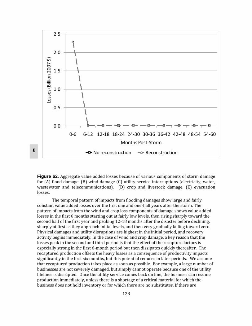
128

Figure 62. Aggregate value added losses because of various components of storm damage for (A) flood damage. (B) wind damage (C) utility service interruptions (electricity, water, wastewater and telecommunications). (D) crop and livestock damage. (E) evacuation losses.

The temporal pattern of impacts from flooding damages show large and fairly constant value added losses over the first one and one-half years after the storm. The pattern of impacts from the wind and crop loss components of damage shows value added losses in the first 6 months starting out at fairly low levels, then rising sharply toward the second half of the first year and peaking 12-18 months after the disaster before declining, sharply at first as they approach initial levels, and then very gradually falling toward zero. Physical damages and utility disruptions are highest in the initial period, and recovery activity begins immediately. In the case of wind and crop damage, a key reason that the losses peak in the second and third period is that the effect of the recapture factors is especially strong in the first 6-month period but then dissipates quickly thereafter. The recaptured production offsets the heavy losses as a consequence of productivity impacts significantly in the first six months, but this potential reduces in later periods. We assume that recaptured production takes place as soon as possible. For example, a large number of businesses are not severely damaged, but simply cannot operate because one of the utility lifelines is disrupted. Once the utility service comes back on line, the business can resume production immediately, unless there is a shortage of a critical material for which the business does not hold inventory or for which there are no substitutes. If there are

0.0

0.5

1.0

1.5

2.0

2.5

0-6 6-12 12-18 18-24 24-30 30-36 36-42 42-48 48-54 54-60

Loss

es (B

illio

n 2

00

7 $

)

Months Post-Storm

No reconstruction ReconstructionE

129

significant lags in recapture, the time-path of BI losses would have an earlier peak and perhaps even be highest in the first period and decline thereafter.

The key initiating factors are the destruction of sector-specific and intersectorally mobile capital stocks in the initial semiannual period, combined with the chilling effect of output losses on economic sector investment, which conspire to reduce the economy’s endowment of capital (and therefore productive capacity) in the second semiannual period. Moreover, it is over this later period that the secondary impacts of storm damage on productivity exert the strongest influence, amplifying losses while contributing to further reductions in investment that perpetuate the effects of the shock. In the model, these fluctuations dampen out by 24-30 months post-storm, at which point the growth of the economy resumes. Nevertheless, the combined long-run effect is to move the economy to a lower growth path, so that without reconstruction through exogenous infusions of capital, business-as-usual levels of output and income are not regained.

Reconstruction is modeled as an exogenous replacement of 50 percent of the destroyed capital stock in the first semiannual period, followed by replacement of the remainder at a constant rate over the succeeding two 6-month periods. It is worth noting that although we assume reconstruction is paid for by insurance and outside aid and, therefore, incurs no drain on financial resources on the part of the California economy, the timing does little to mitigate the run-up in losses in the 6-12 months post-storm because most losses are accounted for by the persistent impacts on productivity as opposed to the initial damage to capital stocks. However, reconstruction does have an attenuating effect on peak losses, and its key benefit is to allow the economy to more rapidly converge to its business-as-usual trajectory, thereby dramatically mitigating the present value of losses over the long run. Table 22 indicates that the latter effect reduces the 5-year costs of utility disruptions by 30 percent and of flood damage by more than 35 percent.

Table 22. Present discounted aggregate impact of various components of storm damage on value added.

[%, percent; $, dollar]

A. Flood damage % Billion 2007 $ Damage Multiplier 2 Year Horizon Without Reconstruction -15.7 -508.8 1.10 With Reconstruction -14.9 -481.7 1.04 5 Year Horizon Without Reconstruction -7.8 -591.5 1.27 With Reconstruction -6.6 -497.7 1.07

B. Wind damage % Billion 2007 $ Damage Multiplier 2 Year Horizon Without Reconstruction -0.04 -1.4 1.02 With Reconstruction -0.04 -1.3 0.94 5 Year Horizon Without Reconstruction -0.02 -1.7 1.23 With Reconstruction -0.02 -1.3 0.96

130

C. Utility service interruptions* % Billion 2007 $ Damage Multiplier 2 Year Horizon Without Reconstruction -3.14 -101.4 1.29 With Reconstruction -3.14 -101.4 1.29 5 Year Horizon Without Reconstruction -1.39 -105.1 1.34 With Reconstruction -1.39 -105.1 1.34 (*electricity, water, wastewater and telecommunications)

D. Crop and livestock damage % Billion 2007 $ Damage Multiplier 2 Year Horizon Without Reconstruction -0.17 -5.3 1.82 With Reconstruction -0.15 -5.0 1.70 5 Year Horizon Without Reconstruction -0.10 -7.3 2.02 With Reconstruction -0.08 -6.2 1.72

E. Evacuation losses % Billion 2007 $ Damage Multiplier 2 Year Horizon Without Reconstruction -0.07 -2.3 0.56 With Reconstruction -0.07 -2.3 0.56 5 Year Horizon Without Reconstruction -0.03 -2.4 0.58 With Reconstruction -0.03 -2.4 0.58

By contrast, the temporal pattern of impacts for utility service and evacuation components of damage is much simpler, concentrated in the first 6 months after the storm and dissipating immediately thereafter. The driving forces that underlie this effect are different. Interruption of electricity, water, wastewater and telecommunications services imposes costs in the form of productivity reductions on the downstream firms that consume these utilities, while any capital stock losses are assumed to be confined to the corresponding upstream sector (for example, damage to cell phone towers, water and sewer mains, electric transmission and distribution assets). Evacuation losses affect industries by rationing the supply of labor, with no capital stock losses at all. The upshot is that at the aggregate level the persistent effect of capital stock losses on the change in overall value added is negligible, and for this same reason reconstruction has no effect on the corresponding economic impacts in this case.

Two features of the results warrant additional explanation. First, the peculiar temporal pattern of losses because of crop and livestock damage is the result of persistent productivity impacts associated with damage to perennial crops that recur on an annual basis, which give rise to a slowly decaying sequence of punctuated losses. This phenomenon arises even in the reconstruction scenario, though the losses there are reduced. Second, the present value of aggregate utilities losses is made up of $54.1 billion reduction in aggregate

131

value added because of water outages, and $27.6 billion and $18.1 billion reductions in aggregate value added because of wastewater and electricity outages, with the remainder due to telecommunications outages.

The labor market effects of the components of damage shown in figure 63 have temporal patterns that resemble the losses in aggregate value added, primarily because of the influence of the aforementioned capital stock dynamics on labor’s marginal product in the various sectors of the economy. Flooded building damage incurs the most severe impacts, inducing a 14 percent reduction in wages and a 6 percent reduction in aggregate employment relative to the baseline trajectory of the economy. Utility service disruptions are a distant second, with reductions in wages and aggregate employment of 4 percent and 7.5 percent, respectively. The magnitudes of the corresponding impacts for the other components of damage are all less than 1 percent.

-16

-14

-12

-10

-8

-6

-4

-2

0

0-6 6-12 12-18 18-24 24-30 30-36 36-42 42-48 48-54 54-60

% C

han

ge f

rom

Bas

elin

e Le

vel

Months Post-Storm

Employment - no reconstruction Employment - reconstruction

Wage - no reconstruction Wage - reconstructionA

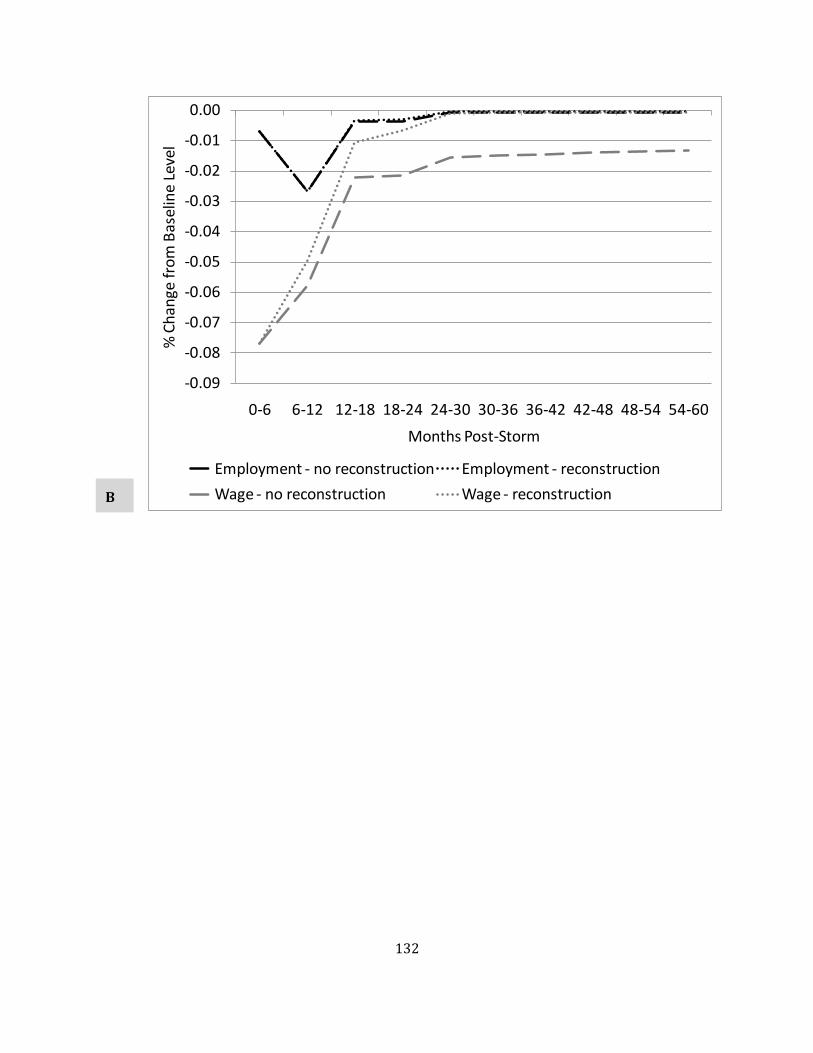
132

-0.09

-0.08

-0.07

-0.06

-0.05

-0.04

-0.03

-0.02

-0.01

0.00

0-6 6-12 12-18 18-24 24-30 30-36 36-42 42-48 48-54 54-60

% C

han

ge f

rom

Bas

elin

e Le

vel

Months Post-Storm


Wage - no reconstruction Wage - reconstructionB

133

-8

-7

-6

-5

-4

-3

-2

-1

0

0-6 6-12 12-18 18-24 24-30 30-36 36-42 42-48 48-54 54-60

% C

han

ge f

rom

Bas

elin

e Le

vel

Months Post-Storm


Wage - no reconstruction Wage - reconstructionC

134

-0.16

-0.14

-0.12

-0.10

-0.08

-0.06

-0.04

-0.02

0.00

0-6 6-12 12-18 18-24 24-30 30-36 36-42 42-48 48-54 54-60

% C

han

ge f

rom

Bas

elin

e Le

vel

Months Post-Storm


Wage - no reconstruction Wage - reconstructionD

135

Figure 63. Employment and wage impacts of various components of storm damage for (A) flood damage, (B) wind damage, (C) utility service interruptions (electricity, water, wastewater and telecommunications), (D) crop and livestock damage, (E) evacuation losses.

Table 23 compares the impact of the various components of damage on the discounted present value of aggregate value added. As was seen in Figure 62, the majority of losses are within the first two years after the storm, and the losses are concentrated in flood and utility service components of damage. The multiplier statistic is the ratio of ex-post value added losses computed by the CGE model to the ex-ante reduction in sectoral gross output that constitutes the direct business interruption impact. With the exception of losses due to evacuation, the multiplier computed on a 5-year horizon is above unity, indicating that the impacts of the shock on the economy’s productive capacity and general equilibrium inter-market price and quantity adjustments are between 27 percent and 129 percent larger than the direct productivity effects on the value of output. (The size of the latter figure, which pertains to crop and livestock damage, indicates the importance of indirect price-mediated substitution effects in downstream industries that use the outputs of agricultural sectors relatively intensively.) This multiplier also highlights the crucial role played by reconstruction in mitigating the economic costs of physical damage, which in the case of flood and wind damage reduces the magnitude of ex-post losses below that of the ex-ante shock. However, this is not the case with components such as utility service disruptions, evacuation losses, and agricultural damage, where destruction of the capital stock plays a minor role and the bulk of the aggregate shock manifests through reductions in industries’ productivity.

-0.10

-0.09

-0.08

-0.07

-0.06

-0.05

-0.04

-0.03

-0.02

-0.01

0.00

0-6 6-12 12-18 18-24 24-30 30-36 36-42 42-48 48-54 54-60

% C

han

ge f

rom

Bas

elin

e Le

vel

Months Post-Storm


Wage - no reconstruction Wage - reconstructionE

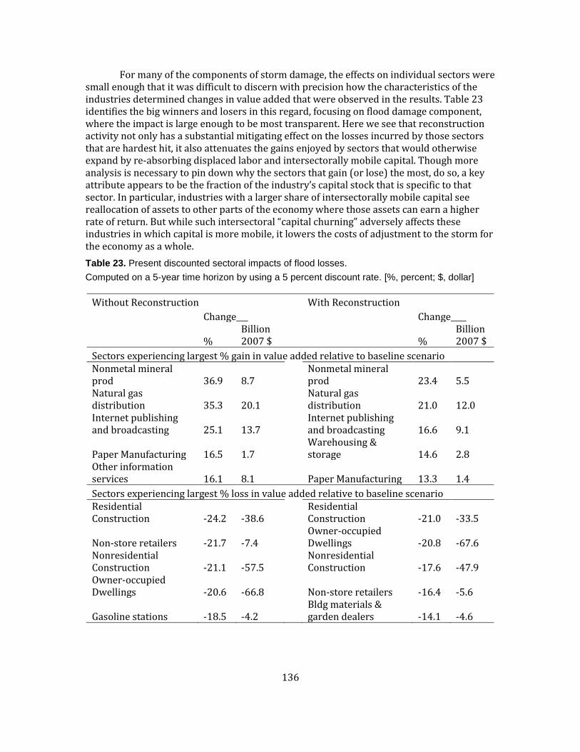
136

For many of the components of storm damage, the effects on individual sectors were small enough that it was difficult to discern with precision how the characteristics of the industries determined changes in value added that were observed in the results. Table 23 identifies the big winners and losers in this regard, focusing on flood damage component, where the impact is large enough to be most transparent. Here we see that reconstruction activity not only has a substantial mitigating effect on the losses incurred by those sectors that are hardest hit, it also attenuates the gains enjoyed by sectors that would otherwise expand by re-absorbing displaced labor and intersectorally mobile capital. Though more analysis is necessary to pin down why the sectors that gain (or lose) the most, do so, a key attribute appears to be the fraction of the industry’s capital stock that is specific to that sector. In particular, industries with a larger share of intersectorally mobile capital see reallocation of assets to other parts of the economy where those assets can earn a higher rate of return. But while such intersectoral “capital churning” adversely affects these industries in which capital is more mobile, it lowers the costs of adjustment to the storm for the economy as a whole.

Table 23. Present discounted sectoral impacts of flood losses.

Computed on a 5-year time horizon by using a 5 percent discount rate. [%, percent; $, dollar]

Without Reconstruction With Reconstruction

Change___ Change____

% Billion 2007 $ %

Billion 2007 $

Sectors experiencing largest % gain in value added relative to baseline scenario Nonmetal mineral prod 36.9 8.7

Nonmetal mineral prod 23.4 5.5

Natural gas distribution 35.3 20.1

Natural gas distribution 21.0 12.0

Internet publishing and broadcasting 25.1 13.7

Internet publishing and broadcasting 16.6 9.1

Paper Manufacturing 16.5 1.7 Warehousing & storage 14.6 2.8

Other information services 16.1 8.1 Paper Manufacturing 13.3 1.4

Sectors experiencing largest % loss in value added relative to baseline scenario Residential Construction -24.2 -38.6

Residential Construction -21.0 -33.5

Non-store retailers -21.7 -7.4 Owner-occupied Dwellings -20.8 -67.6

Nonresidential Construction -21.1 -57.5

Nonresidential Construction -17.6 -47.9

Owner-occupied Dwellings -20.6 -66.8 Non-store retailers -16.4 -5.6

Gasoline stations -18.5 -4.2 Bldg materials & garden dealers -14.1 -4.6

137

SUMMARY OF RESULTS

The major economic results of our study are presented in table 24. The first part of the table summarizes property damage calculated earlier in the report, while the second collates the business interruption losses.

Table 24. Summary of ARkStorm costs and business interruption. With recapture and without reconstruction

a) for California over a 5-year time horizon.

[in billions of 2007 U.S. dollars]

Property repair/ reconstruction cost

Business Interruption

Building Flood Damage $195.0b $591.5 Related Content Damage 103.0 Building Wind Damage 5.6 1.7 Agricultural Damagec 3.6d 7.3 Power System Damage 1.0e 18.1 Telecommunication System Damage 0.1 5.2 Wastewater System Damagef 0.3 27.6 Water System Damageg 3.0h 54.1 Highway/road Damagei 2.5j 0.02k Levee Repair and Island Dewateringl 0.5 n.a.m Evacuation 2.4 Relocation 39.0n n.a.o Total 353.6 707.9 Total After Double-Counting Adjustment 353.3 627.4

a Results for the case “without reconstruction” are used in this summary because they report the gross damage from the event; the “with reconstruction” case includes an offsetting stimulus and gives a misleading picture of losses from the hazard when most of the funding comes from outside of the region.

b Weather and flood warning (of at least 48 hours) could reduce building damages by $30 billion, while demand surge could increase property repair costs by $70 billion. (See section on Building Content and Repair Costs).

c Agricultural costs pertain to field damage, crop, and livestock replacement, and forgone income from crop losses. d Agricultural losses increase to $6.8 billion for high end range of flood duration estimate. e Power system repair cost estimates range from $0.3-$3 billion. f Wastewater system repair costs pertain to sewer pipe damage. g Water system repair costs pertain to electric equipment and well damage. h Water system repair cost estimate ranges from $1-10 billion. i Highway/road repair cost pertain to landslide damages. j Highway repair cost estimate ranges from $2-3 billion. k Economic impacts from reduced highway capacity pertain to truck traffic in California only. l Levee repair and dewatering costs pertain to the levees and islands in the Delta area only. m Potentially, levee repair and island dewatering time would increase business interruption losses through increased

agricultural damages. n $39 billion relocation costs calculated by using HAZUS-MH formulas, $25 billion for relocation of residences and $11

billion for relocation of commercial establishments, and the remainder for industry, education, religion, and agricultural occupancy classes.

o The positive effects of relocation have not been evaluated; building service interruption time multipliers have not been developed for the flood module of HAZUS-MH

138

The ARkStorm scenario presents a flood catastrophe and wind disaster. Hundreds of billions of dollars of building damages can cause even greater hundreds of billions of dollars of business interruption losses because of building downtimes of one to three years. These downtimes were lengthened by the inclusion of add-ons such as drying out the buildings, permitting and dealing with hazardous waste. In contrast, the shorter building downtimes from wind damages result in business interruption losses that are less than the wind damage property repair and replacement costs.

The business interruption losses from lifeline outages depend on the spatial scale of the outages, the time to restore service, the importance of the lifeline service to operations, and the availability of substitutes. Water and power lifelines cause the greatest business interruptions: the water supply system is presumed to have longer restoration times than the other lifelines and power system outages, affecting all counties, are more widespread than the other lifelines. However, consideration of double counting reduces the business interruption loss contribution from water such that power causes more business interruptions than water after adjusting for double counting. This loss is because of more spatial correlation of flooded building damages with water outages than power outages. The ratio of business interruption losses to replacement cost is highest among the lifelines reinforcing the importance of critical infrastructure to the macro economy.

Agricultural business interruption losses are only slightly larger than soil and crop damage. The impact of evacuation is quite small because we only isolated the flood duration component of evacuation time. We considered the impact of highway damages on truck traffic only, in terms of increased shipping costs because of increased travel time, though these costs are moderated by the redundancy in the highway network

The $327 billion in business interruption from ARkStorm would make this the costliest disaster in the history of the U.S. For example, business interruption from the ShakeOut Earthquake Scenario is estimated to be about $67 billion, from the World Trade Center attack a maximum of $100 billion, and from Hurricane Katrina currently (2010) $100 billion (though still rising because recovery has not been completed). The magnitude is a combination of the intensity of the storm, the vulnerability of the site in terms of a large asset base that is ill protected from this kind of event, and its large areal extent.

CONCLUSION

We have estimated the economic impacts of ARkStorm to be several hundred billion dollars over a five-year period. At the same time, we offer many caveats to the economic analysis. There are limitations in scope (for example, levee repair estimates for the Delta region only, impacts of transportation for highways/roads and truck traffic only), gaps in knowledge (for example, lack of building service interruption time multipliers for flood damaged buildings), and uncertainties in the cost estimates (noted as ranges for lifelines and agricultural damages, and as adjustments for warnings and demand surge in the notes for (table 24)) are two. However, the relative order of magnitude of the results is likely representative of the domination of flooded building damages and economic impacts followed by lifeline services, water service in particular. Although agricultural and transportation damages and impacts are estimated as relatively light, they are on a much greater scale than experienced during previous California storms. Similarly, the scale of evacuation would be unprecedented for California. Sensitivity analysis will be used in the next stage of the research to explore the effects of the uncertainties in the damage and restoration estimates.

The novel aspect of this study is the use of a computable general equilibrium approach to systematically characterize and quantify the economic consequences of the full spectrum of

139

individual but overlapping impacts of a large-scale natural disaster. Cost estimation based on the full spectrum of individual impact categories is not new in large-scale disaster research, as, for example the ShakeOut earthquake scenario study (Jones and others, 2008; Rose and others, written commun.). However, the input-output approaches utilized by ShakeOut and similar studies (Okuyama and Chang, 2004; Okuyama, 2007) have difficulty capturing the feedback effects of property damage, temporary interruptions in labor supplies, and hysteretic adverse productivity shocks on prices, producers’ and consumers’ substitution responses, and concomitant intersectoral supply-demand adjustments across the economy. Distinctly, prior CGE analyses of the effects of disasters either limit consideration of impacts to a fairly narrow range of damage categories (Rose and Liao, 2005; Rose and others, 2007), or express the shock to the economy in a highly aggregate fashion with little differentiation among different types of damage (Selcuk and Yeldan, 2001), potentially leading to under- or double-counting of impacts (respectively) and the associated macroeconomic costs. Bearing these issues in mind, our key contribution is the development of algorithms for translating the outputs of geospatial engineering models of disaster damage (HAZUS-MH) into sequences of shocks to capital stocks and productivity in various industry sectors, and to aggregate together the resulting general equilibrium economic cost impacts in a way that controls for the overlapping effects of different categories of damage. (A useful point of comparison is Rose and others (2009) alternative approach of specifying BI losses directly as constraints on the outputs of CGE model sectors.) By addressing several of the methodological concerns outlined in Rose (2004a) and Okuyama (2007), the current advance provides a roadmap for refining future estimates of both the macroeconomic costs of disasters and the mitigating influence of resilience.

Truck Traffic Economic Impacts from Reduced Highway Capacities

Closed highways and reduced highway capacities because of landslide and flooding damages will affect emergency responder access and commuter and truck routes. Analytical methods to analyze effects of extreme weather on the performance of the transportation system is not well developed. For the ARkStorm scenario, we attempted an economic impact analysis of large truck traffic. We obtained technical support from various University of Southern California-affiliated independent consultants through Hanh Dam Le Griffin (TTW, Inc.). Their transportation model analyzed the effects of reduced highway capacities on the regional and national movement of goods and services by estimating changes in truck distance, travel time, and associated costs and the impacts of increased shipping prices on major economic sectors. Despite the sophistication of this modeling system, we identified various issues with its application to a winter storm event and determined some of the research needs for transportation modeling.

Method of Analysis

The state and national highway network was analyzed for 4 points in time following the southern California storm: on day 3, day 14 (one day after the northern California storm), day 90, and day 180. The highway capacities on these days are explained and mapped in the highway damage section of this report. Independent model runs were conducted for the southern and northern storm events —generating a total of seven model runs for the analysis. (Note that highway damages from the northern California storm have not yet occurred on day 3.)

A model run on the national highway network is comprised of three principal models: a national highway network model, a transportation cost model, and a demand-driven national interstate economic model (the National Interstate Economic Model (NIEMO) and an elaborated TransNIEMO) that have been developed by the consultant group (Park and others, 2005, 2007,

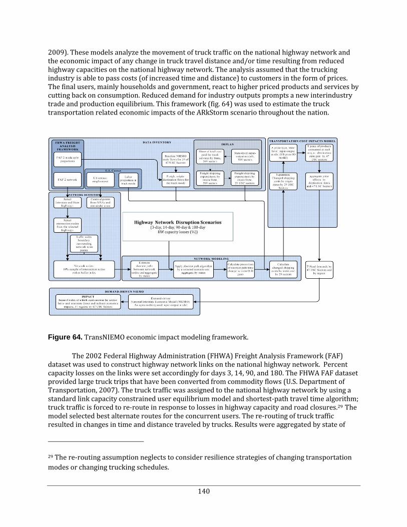
140

2009). These models analyze the movement of truck traffic on the national highway network and the economic impact of any change in truck travel distance and/or time resulting from reduced highway capacities on the national highway network. The analysis assumed that the trucking industry is able to pass costs (of increased time and distance) to customers in the form of prices. The final users, mainly households and government, react to higher priced products and services by cutting back on consumption. Reduced demand for industry outputs prompts a new interindustry trade and production equilibrium. This framework (fig. 64) was used to estimate the truck transportation related economic impacts of the ARkStorm scenario throughout the nation.

Figure 64. TransNIEMO economic impact modeling framework.

The 2002 Federal Highway Administration (FHWA) Freight Analysis Framework (FAF) dataset was used to construct highway network links on the national highway network. Percent capacity losses on the links were set accordingly for days 3, 14, 90, and 180. The FHWA FAF dataset provided large truck trips that have been converted from commodity flows (U.S. Department of Transportation, 2007). The truck traffic was assigned to the national highway network by using a standard link capacity constrained user equilibrium model and shortest-path travel time algorithm; truck traffic is forced to re-route in response to losses in highway capacity and road closures.29 The model selected best alternate routes for the concurrent users. The re-routing of truck traffic resulted in changes in time and distance traveled by trucks. Results were aggregated by state of

29 The re-routing assumption neglects to consider resilience strategies of changing transportation

modes or changing trucking schedules.

141

origin and destination and reported for California, other states combined, and all of the national highway network.

Next, the effects of changes in total truck travel time and distance on trucking costs were assessed for (49) states across 29 commodity sectors30 by using the transportation cost impact model based on a cost-price input-output model. The difference in trucking time and distance was converted to dollars by summing the variable costs of time ($17per hour labor rate) and distance (for example, $0.48/mile) (Berwick and Farooq, 2003)31. The increased shipping costs from the state of origin (i) to the state of destination (j) for industry sector (k, k=1…29) were aggregated by the state of destination. Total truck costs (measured in millions of dollars per year were summarized for California, other states combined, and a total for the U.S. Finally, based on changes in total shipping costs for the 29 University of Southern California commodity sectors, a destination-state cost-price input-output model measured the effect of price increases on 47 economic sectors in 49 destination states. The model assumed that 100 percent of increased shipping costs were passed on to customers as increased prices for goods and services at the destinations, which results in decreased consumer demand for goods and services. The NIEMO estimated direct and indirect economic damages associated with changes in consumer demand at the destination states. The economic impacts (measured in millions of dollars of industry output) were aggregated by destination state for each scenario and summarized for California, other states combined, and the U.S.

Truck travel time, distance, cost, and economic impacts

Change in truck travel time and distance: table 25 and table 26 present differences in truck travel time and distance, relative to the 2002 baseline, for each model run received from TTW, Inc. Overall, increases in truck travel time results from the re-routing that occurs in response to ARkStorm highway capacity reductions and closures. Most of the California truck travel time increases occur from the southern California storm reflecting the severe capacity losses of the highway network in southern California on day 3 and also the region’s significant trade volume and goods movement activities. On Day 14, the increase in truck travel time in the south is reduced following restored highway capacities on some routes affected by flooding and erosion and landslides. Truck travel is less affected by the northern storm, but as noted under the study limitations, route 99 was allowed to operate at full capacity when it should have been closed. Re-routing increases travel time throughout the rest of the country, but the use of alternative routes

30 The models utilize common-denominator aggregations of standard economic classifications

(including NAICS, SIC, and others), called the University of Southern California Sectors. There are

47 University of Southern California Sectors, 29 of which are commodity sectors. The commodities

are shipped, but the availability can affect the remaining sectors. Therefore, first-order network

effects are reported for 29 sectors, but full effects are reported for all 47 sectors.

31 The equation to calculate truckers’ labor cost per mile in appendix A of Berwick and Farooq

(2003) assumes that the Labor (Wage) Rate per Hour (LRPH) is $10 per hour. For this analysis the

current (2010) LRPH is updated to $17 per hour yielding a trucker’s labor cost of $0.09 per mile.

Other variable costs are $0.48 per mile such that the estimated labor cost is 65 percent of the total

variable cost (0.65 = 0.9 / (0.9+0.48)).

142

actually decreases the total truck travel distance in the other states. Some routes experience less congestion and a corresponding gain in traffic flow.

Table 25. Change in highway network truck travel time. 2002 FHWA Freight Analysis Framework (FAF) data as baseline. Aggregated to spatial unit by network origin and destination.

Region Truck Travel Time Increase (in Hours)

Day 3 Day 14 Day 90 Day 180

Southern California storm 231.0 17.0 0.3 zero

Northern California storm n/a 37.8 1.3 1.1

TOTAL California 231.0 54.8 1.5 1.1

OTHER STATES 899.3 410.5 44.3 4.5

TOTAL U.S. 1,130.3 465.4 45.8 5.6

Table 26. Change in highway network truck travel distance.

2002 FHWA Freight Analysis Framework (FAF) data as baseline. Negative signs denote a decrease in truck miles. Aggregated to spatial unit by network origin and destination.

Region Truck Travel Distance Increase (in Miles)


Southern California storm 8027 1,968 75 zero

Northern California storm n/a 1,063 97 194

TOTAL California 8,027 3,031 173 194

OTHER STATES -63,312 -3,105 -2,215 -878

TOTAL U.S. -55,285 -74 -2,043 -684

Figure 65 and figure 66 display the change of network volumes on day 3 from the southern California storm, and day 14 from the northern California storm, respectively. On Day 3, the southern California network link volumes experience substantial percentage changes, especially on the Ventura Freeway (U.S. 101 and route 134) east-west route through Ventura County and in the southern San Fernando Valley in Los Angeles County. However, the effects are not limited to southern California, as indicated by the percentage volume changes in the rest of country, albeit of a much smaller scale. On day 14, in northern and central California, there is a high percentage decrease in network link volumes in Sacramento, the Bay Area, and the Central Valley. Similar to the results of the southern California storm event, the impacts are not limited to just the northern and central regions of the state, but at a smaller scale to southern California and other states. For traffic volumes traveling between a specific pair of origin and destination points in the national network, ARkStorm highway capacity changes will result in some volume decreases along certain links, and countervailing increases in volume along alternative links.

143

Rough extrapolation of the 4 day results to the 6 month period following ARkStorm suggests that the total number of truck miles reduces by about 600,000 miles because of re-routing: the truck miles increase by 100,000 miles in California and decrease by 700,000 miles throughout the rest of the U.S. However, total truck travel time increases by 18,000 hours: truck travel time increase by 15,000 hours outside of California and most of the 3,000 hour truck travel time increase in California is associated with the southern California storm. These results suggest that while both truck travel distances and time would increase within California, trucking costs outside of California could involve a trade-off between fewer miles travelled and longer travelling times.

Figure 65. National highway network volume change for southern California storm on day 3.

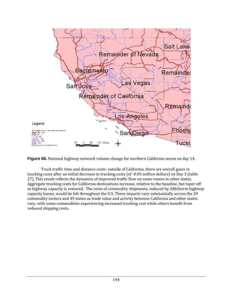
144

Figure 66. National highway network volume change for northern California storm on day 14.

Truck traffic time and distance costs: outside of California, there are overall gains in trucking costs after an initial decrease in trucking costs (of -0.05 million dollars) on Day 3 (table 27). This result reflects the dynamics of improved traffic flow on some routes in other states. Aggregate trucking costs for California destinations increase, relative to the baseline, but taper off as highway capacity is restored. The costs of commodity shipments, induced by ARkStorm highway capacity losses, would be felt throughout the U.S. These impacts vary substantially across the 29 commodity sectors and 49 states as trade value and activity between California and other states vary, with some commodities experiencing increased trucking cost while others benefit from reduced shipping costs.

145

Table 27. Change in trucking costs.

Costs are aggregated to spatial unit by geographic destination.

Time is valued at $17 per hour; distance is valued at $0.48 per mile.

Impact on truck costs associated with 29 commodity sectors (excluding service sectors).

Negative sign denotes a decrease in truck costs for commodity shipments.

[n/a, not applicable]

Region Total Trucking Costs (in millions of dollars)


Southern California 2.2 0.7 0.0 0.00

Northern California n/a 0.6 0.1 0.03

TOTAL California 2.2 1.2 0.1 0.03

OTHER STATES 0.0 0.8 0.3 0.01

TOTAL US 2.2 2.0 0.4 0.04

Rough extrapolation of the 4 days to 6 months suggests that trucking costs increase on the order of $60 million dollars: $38 million in California with 75 percent of the cost increases associated with the highway damages from the southern California storm and $22 million trucking cost increases in other states.

Truck traffic economic impact: The total (direct and indirect) economic impact, measured in terms of industry output losses (in millions of dollars), is associated with trucking cost changes only.32 Table 28 presents estimates of the economic impacts of reduced highway capacities from the ARkStorm scenario for each of the 4 days. Table 28 is not a simple and direct reflection of changes in trucking costs (table 27) because of consumer responses to changes in prices.

32 Other economic impacts that may occur as a consequence of highway network disruption

associated with California storm events were not accommodated.

146

Table 28. Truck traffic economic impact. Aggregated by geographic destination. Time value at $17 per hour; distance value at $0.48 per mile. Negative signs denote a gain in economic output. [n/a, not applicable]

Total impact (in millions of dollars of output)


Southern California 1.1 0.3 -0.03 0.00

Northern California n/a 0.3 0.03 -0.04

TOTAL California 1.1 0.6 0.00 -0.04

OTHER STATES 0.2 0.8 0.34 0.09

TOTAL US 1.3 1.4 0.34 0.06

The economic impact of the ARkStorm highway capacity reductions is evident throughout the nation. The national aggregation of results suggests that there are output losses, although there are slight output gains in California (estimated at $30,000 for Day 90 in southern California and $40,000 for Day 180 in northern California) as highway conditions improve. Other states also experienced output gains (where substitution of pricier commodities favored some sectors in some states) that were offset by output losses in other states. Therefore, given the fixed interindustrial and trade relationships (of the NIEMO model) economic impact in some states can positively affect the economy in California through the industrial links and domestic trade activities of these states with California. For California, the largest gains in economic output were reported for the motorized and other vehicles sector. The sectors with the largest output losses included construction, other services, wood products, electronics, real estate, and accommodation and food services.

Rough extrapolation of the 4 day analyses suggest that output losses for California are on the order of $16 million and are mostly attributed to the southern California storm. Output losses of $27 million in the rest of the U.S. adds up to a $43 million economic impact to the U.S. economy from ARkStorm highway network disruptions. These economic impacts are an order of magnitude less than the $500 million estimates of delayed and lost automobile and truck trip costs calculated for the ShakeOut earthquake scenario in the southern California region (Jones and others, 2008). Conversely, the costs of ARkStorm highway repairs of $2.5 billion are an order of magnitude greater than the repair cost estimate of $400 million for the ShakeOut scenario. We conclude that while the highway truck transportation model accommodates the scale of California and the rest of the country, various compromises very likely have underestimated the economic impacts of the ARkStorm highway capacity reductions.

RESEARCH NEEDS RELATED TO TRAFFIC ECONOMIC IMPACTS

Overall, despite the accomplishment of applying a state-of-the-art highway model to analyze the ARkStorm highway capacity reductions, budget and time constraints did not permit further investigation of the limitations and research gaps that were identified. First, the analysis was

147

challenged by the hundreds of highway capacity alterations from ARkStorm landslides and flooding. These analyses were aggregated to reduce the burden on data entry. During this process, it appears that flood related capacity reductions along California 99 between the Grapevine and Sacramento were overlooked; Day 14 conditions would not likely allow the re-routing and volume increases along this highway. Highway closures and capacity reductions along California 99 would increase truck travel time, distance, and costs, and economic impacts. Second, independent model runs of the northern and southern storms have missed interactive effects of the damages from the two storms on truck travel and will have further underestimated the impacts of truck distance, time, associated costs and price feedbacks. Third, the analysis of four days captured the impacts as snapshots in time so that it was necessary to coarsely extrapolate to the six-month period following the winter storm scenario. Fourth, we took stock of highway damages and capacities at the conclusion of each of the southern and northern storms. Therefore, we have not captured all the phases of a severe storm. Precipitation, wind, and wave surge in coastal areas that precede inundation or actual closure of roadways would also effect highway operations and safety in the form of travel delays. Fifth, the model, as complex as it is, only implements the resilience strategy of re-routing. Other strategies such as change of travel time (for example, travelling through the night) or change of transportation modes (to rail or air) were not considered. Beyond a price response, industrial sector resilience strategies for supply chain disruptions were not incorporated. Sixth, the result of reduced truck distances and increase miles needs further exploration and explanation. Although equilibrium-based network models are appropriate for uncongested urban network when travel time is a function of volume, and traffic demand is spread over many alternative routes in such a way to equalize volume-sensitive travel times on each of the routes, the application to the interstate network requires caution. Furthermore, equilibrium–based network models have been used to analyze investment scenarios that add capacity or enhance performance, rather than degrade it in the case of disasters. Reduced highway capacity can create impossible optimization problems if a subnetwork is totally isolated from the network. (Sungbin Cho, Southern California Association of Governments, written commun., 2010) Seventh, explanation of the effects on the different sectors would be insightful. Eighth, the models used to analyze economic impacts were developed to deal solely with truck traffic and movement on the national highway network. Therefore, for this and various other reasons, stated above, the results for the ARkStorm scenario (table 24) understate the potential economic impacts of reduced highway capacities from such storms.

The ARkStorm scenario would affect the mobility of automobile and emergency vehicles, and further studies and additional data would be required to assess these impacts in any detail. In principle, the impacts on automobile and emergency vehicles would reflect those estimated for truck traffic. Because of highway capacity losses and road closures, automobiles and emergency vehicles also would be forced to re-route to avoid congestion or to reach their destinations. As result of re-routing, travel delays would likely occur and be measurable on a value of time and distance basis. In addition to re-routing, depending on trip type and purpose, some commuters and travelers might switch to alternative modes, such as public transit; some may be able to telecommute; and some travelers may decide not to travel. These decisions could alter the number and timing of automobile trips on the national highway, and consequently traffic flows in some parts of the network may experience relief. The response of auto travelers to highway capacity losses and road closures are somewhat similar to those of trucks, although automobile and small truck trips have more flexibility than large truck trips that tend to be more time sensitive and have fewer routing and alternative modes of transportation. In addition, emergency vehicles and also some trucking companies may have designated alternative routes and may not react to time, cost, and congestion alone. The consequences of delay or an inability to travel or effectively respond to

148

emergency situations, could potentially be substantial. Any quantitative measure and confirmation of these impacts would require further in-depth study.

Finally, for future analysis of storm events in the broader context of climate change, further development of transportation models for conditions of reduced highway capacities and closures are needed to inform planning decisions about industrial locations and emergency plans. Linkages to environmental impacts of extreme weather in terms of fuel use and greenhouse gas emissions could also be made. (Reza Navai, California Department of Transportation, written commun., 2010)

Environmental and Health Issues

This section is an abridged version of a much more detailed report (G. Plumlee and C. Alpers, USGS, written commun., 2010). The rainfall, snowfall, erosion, flooding, landslides, winds, and resulting physical damage to infrastructure from an extreme storm such as that modeled by ARkStorm could result in substantial physical and chemical stresses on the environment, with resulting impacts on the health of affected ecosystems and humans. The framework developed for the ARkStorm meteorology and physical impacts can be integrated with a wide variety of information to infer plausible scenarios for environmental, ecological, and environmental-health impacts of the hypothesized storm.

PLAUSIBLE ENVIRONMENTAL-HEALTH ISSUES AND IMPACTS

Severe storms can pose diverse and significant physical threats to human safety. Common results of these threats include, for example, drowning in flood waters and injuries or death caused by hypothermia, tornadoes, floodwater-borne debris, lightning strikes, rainfall-triggered landslides or rockfalls, avalanches, and wind-related damages (such as falling trees or power lines), and fires from petroleum products released into floodwaters. These hazards deservedly receive the bulk of public-health focus during active storms, and a detailed analysis of plausible ARkStorm impacts in this realm should prove extremely useful, but is beyond the scope of this study. The focus of our analysis from a public-health perspective is on plausible environmental-health impacts, meaning those shorter- to longer-term health issues that result from environmental exposures.

Our analysis is based in part on inferences that can be drawn from peer-reviewed publications summarizing environmental and environmental-health impacts documented or postulated from past storms and floods, both in California and elsewhere. Based on this type of analysis, a wide variety of plausible environmental issues must be considered for ARkStorm.

Storm runoff, particularly in those areas receiving high hourly rainfall rates and areas in which rain falls on pre-existing snow, would likely lead to widespread erosion, transport, and redistribution of soils, sediments, and rock materials. The physical impacts alone of these materials on riverine, floodplain, lacustrine, and coastal environments could be substantial and could lead to significant impacts on species habitat and loss of life in some aquatic or terrestrial organism populations.

Some rock types, and the soils developed on them, may contain naturally elevated levels of potentially toxic metals (such as selenium, zinc, copper, arsenic, and lead), environmentally deleterious minerals (such as iron sulfides that generate acid rock drainage when weathered), mineral toxicants (such as asbestos), or pathogens (such as Coccidioides Immitis, the soil fungus that causes Valley Fever). Storm-induced erosion or landslides affecting these rock types have the potential to disperse these materials in the environment.

149

Storm or flood damage to buildings, infrastructure, industrial facilities, or agricultural facilities (such as wastewater treatment plants, petroleum refineries, active or inactive mines, chemical manufacturing plants, animal feeding operations, and others) could release debris, contaminants, and microbial pathogens into the environment. Erosion or flooding of agricultural lands could lead to extensive loss or contamination of arable soils. Storm runoff from agricultural lands, residential areas, and urban areas could release a variety of sediment-borne or water-borne anthropogenic contaminants into the environment. Water supplies used for human consumption, livestock consumption, or agricultural irrigation, including surface water and shallow groundwater, could become contaminated by a wide variety of contaminants or pathogens. Following the storm, contaminated sediments and debris redistributed by landslides or floodwaters could then dry out and become available for further redistribution by human disturbance and (or) wind transport.

In addition to the acute physical threats to safety posed by the storm, the possibility exists for adverse health effects on humans and ecosystems. These effects could include, for example, potential outbreaks of infectious disease from exposure to contaminated floodwaters, consumption of contaminated drinking water, or exposure to dusts from landslide or flood deposits containing soil pathogens such as Coccidioides Immitis. In most developed countries, effective health hazard communication and preventive emergency response measures (such as warnings not to drink potentially contaminated water and providing access to uncontaminated water) commonly prevent or substantially lessen the magnitude of many infectious disease outbreaks. However, as shown in this report, widespread flooding and damage to infrastructure could reduce the ability of emergency responders to provide basic services in the timeframe needed to avoid at least some infectious disease occurrences; an example would be the challenges of providing fresh drinking water to large numbers of people across broad storm-affected areas.

APPROACH FOR ENVIRONMENTAL AND HEALTH IMPACTS

While the list of plausible environmental and environmental-health issues that could result from ARkStorm is substantial, a much more detailed analysis of each issue is needed to determine the likelihood of whether it would actually occur and, if likely, the magnitude of the potential impacts. While detailed analyses of all potential issues are well beyond the scope of this study, we have outlined and begun to test an approach by which such analyses can be made.

Further insights about potential geogenic (natural) and anthropogenic sources of storm-induced environmental contamination can be gleaned by linking ARkStorm precipitation and flooding maps to data extracted from diverse database sources with geologic, hazards, and environmental information. Guided by results of such analyses, site-specific or other types of investigations can be developed to assess in more detail the potential occurrences and magnitude of the issues in question. Two examples are discussed briefly here: linkages of ARkStorm precipitation and flooding data to (1) environmental lithology databases and (2) National/State scale environmental facilities databases.

Linkages to environmental lithology maps. Environmental lithology maps can be derived from State digital geologic map databases to show the distribution of rock types that could serve as nonpoint sources for potentially hazardous materials released into the environment as a result of ARkStorm-triggered runoff and erosion. For example, certain types of rocks naturally contain high levels of iron sulfides (pyrite, FeS2, also known as fool’s gold) and trace metals such as copper and zinc. Weathering and oxidation of these rocks can produce natural acid-rock drainage with a wide variety of elevated metals that can be detrimental to aquatic organisms. Watersheds where abundant outcrops of these rock types coincide with high rainfall or snowmelt (such as ARkStorm) would, therefore, be at higher risk for storm-related release of acid-generating rocks by landslides

150

or erosion into downstream areas, amplifying the environmental impacts of the natural acid-rock drainage. However, it is likely that such effects would be localized largely in the watersheds close to where the rocks outcrop. Another example that has occurred elsewhere is the storm-related dispersal of asbestos into the environment from landslides in ultramafic rocks; however, the effects likely would be restricted to areas relatively close to the ultramafic rock outcrops.

Linkages to national- or state-scale facilities databases. A variety of state- to national-scale facilities databases can provide useful insights into the locations and types of industrial or other facilities with some potential for storm-related releases of contaminants into the environment. Examples of useful databases include the U.S. Environmental Protection Agency (EPA) Facility Registry System (FRS) database, State databases of land use and facilities such as animal feeding operations, and various USGS databases on historic and active sites of mining or mineral processing.

Wastewater treatment plants (WWTPs) are an example of a facility type that can be examined linking state- or national-scale databases to ARkStorm flooding and precipitation maps. As discussed earlier , WWTPs are more likely to be located in flood-prone areas, because the need to minimize pumping dictates that these plants be located at the lower elevations of the respective sewage system service areas. An analysis of the EPA regulated facilities database for California, in which WWTPs were extracted by using the key words or phrases “sewage”, “sewerage”, or “WWT”, identified more than 900 facilities across the state. Of these, a substantial fraction are predicted to be either within the plausible zone of ARkStorm flooding, or in predicted zones of maximum daily precipitation rates well in excess of 4 inches per day. Either result would likely lead to release of raw or partially treated sewage or other wastewater (along with contained contaminants and pathogens). Therefore, release of contaminated wastewater from flooded, shut-down, or overloaded WWTPs is a plausible and substantial environmental impact that likely would result in some areas of the State; geospatial analysis of the results highlights areas that are of higher concern than others. Such releases are commonly observed as a result of floods in the U.S. and worldwide, but effective hazards communication and preventative actions by emergency responders can substantially reduce the potential human health impacts. Further examination is warranted, however of potential ecological impacts from flooded WWTPs and other environmentally significant facilities near flood-prone areas. Many of the lowland, riparian, or lacustrian areas where floodwaters accumulate also are home to a wide variety of aquatic and terrestrial wildlife that could be affected adversely by floodwater-borne contaminants or pathogens.

Limitations: There are some substantial limitations in this approach that must be recognized and the appropriate caveats placed on interpretations and conclusions. A reconnaissance survey of a number of the databases used in the analysis reveals relatively common issues, such as incompleteness of coverage (for example, known facilities are missing), duplicate entries with different locations, and inaccuracy of geospatial location information for individual facilities of concern. Also, many databases lack specific information about the types of environmental contaminants that potentially could be released during an ARkStorm-scale event from specific source facilities. As a result, without extensive efforts to address such limitations, the use of state- to national-scale databases to map potential sources of storm-induced environmental contamination should be considered qualitative at best. Nevertheless, this qualitative approach does provide much useful information and also helps to fulfill a primary goal of this study, which is to identify areas where improvement in the approach for estimating plausible impacts is needed.

151

Public Policy Issues

Stated simply, public policy can be described as a predisposition of governments to act in a predetermined manner, although in actuality it is “whatever governments choose to do or not to do” (Newell, 2004, p. 153). Public policymaking in the U.S. is the responsibility of elected bodies, such as city councils, state legislatures, and the U.S. Congress. Managers of federal, regional, state, county, and city agencies also participate in policymaking, helping conceptualize and create policies. The policymaking process tends to evolve in response to societal or community problems perceived by citizens, interest groups, and political leaders. In a governmental context, it can be described as a cycle of (Newell, 2004, p. 153):

Agenda setting, when issues are brought to the attention of policymakers,

Policy formulation, when options are considered and a course of action is adopted,

Implementation, when adopted policies are put into action, and

Evaluation, when a policy assessment is performed, and ways to modify or improve policies are provided.

In the context of this policymaking process description, the ARkStorm policy assessment largely corresponds with the agenda and policy formulation stages. This assessment looks at the priority public policy issues highlighted by the ARkStorm scenario. These priority issues are organized around the basic functions of disaster management—mitigation, preparedness, response, and recovery, as well as risk awareness—a major behavioral factor in disaster management. In addition, this assessment also identifies an overarching policy consideration and identifies possible courses of action.

OVER-ARCHING POLICY CONSIDERATION

The ARkStorm scenario hypothesizes a disaster of catastrophic proportions for which existing national and state disaster policies are ill suited. Over the last 60 years, U.S. disaster policy agenda setting and policy transformations have occurred mostly during relatively brief periods of time – usually following disastrous events (Birkland, 2006; Rubin 2007). As Birkland advises “a disaster can often do in an instant what years of interest group activity, policy entrepreneurship, advocacy, lobbying, and research may not be able to do” (Birkland, 2006, p. 5). But, having relatively few major urban disasters within this timeframe suggests that these event-related policy changes mostly reflect the learning from far more moderate disasters.

The modern U.S. disaster management system works as a shared system in which over 88,000 local governments, special districts, and Native American tribal governments have primary responsibility for supplying disaster-related resources; federal, regional, and state agencies are to provide support as requested (Federal Emergency Management Agency, 2005). This shared system is triggered from the “bottom-up.” Local governments are aided, as needed, by states, and both are aided, in turn, by the federal government. By design, the system requires extensive coordination and cooperation among all levels of government, as well as the many private organizations involved in disaster management. This process is also an incentivized system of partnerships, in that states and localities are encouraged, but not required, to participate.

Table 29 generalizes the current (2010) disaster policy framework in the U.S. for the basic disaster management functions, combining preparedness and response, and adding risk awareness. The basic role and responsibility of each level of public policy making—federal, regional, state, county, and localities—plus the private sector are described briefly. Some of the key policies evaluated in this assessment are articulated in the following legislation, doctrine, and programs:

152

National Flood Insurance Program (NFIP) provides flood insurance through the private sector, with backing by the federal government. Insurance also is reinforced by 100-year and 500-year floodplain mapping, together with rate reductions in relation to local government mitigation actions. Various types of flood mitigation and project grants also are administered. The NFIP represents the national position on “shared-risk.” The government will help, but the aim is to encourage local governments and individuals to share flood risk.

Robert T. Stafford Disaster Relief and Emergency Assistance Act (Stafford Act) provides for individual and household assistance post-disaster, Public Assistance grants to restore damaged public facilities and infrastructure, and mitigation grants that fund both local hazard mitigation planning and projects to help strengthen communities against future disaster losses. Interacting with Stafford Act programs are the National Incident Management System (NIMS), providing a standardized nationwide protocol for managing response at each level of government, and the National Response Framework (NRF), which coordinates disaster response among federal agencies. These directives help further define federal response, recovery, and preparedness doctrine. The Post-Katrina Emergency Management Reform Act (PKEMRA) of 2006 modified the Stafford Act. PKEMRA directed FEMA to develop both a National Disaster Recovery Strategy and National Disaster Housing Strategy. FEMA finalized the National Disaster Housing Strategy in January 2009 (http://www.fema.gov/pdf/media/2009/ndhs.pdf). The National Disaster Recovery Framework (http://disasterrecoveryworkinggroup.gov/ndrf.pdf) is still under development.

Disaster Mitigation Act of 2000 (DMA 2000) requires local adoption of a FEMA-approved Local Hazard Mitigation Plans (LHMP) as a precondition for receipt of federal mitigation project grant funding. The act also provides a competitive Pre-Disaster Mitigation (PDM) grant program to fund local hazard mitigation planning efforts and mitigation projects.

State and local government programs include state and local emergency planning and use of the Incident Command System (ICS)/Standardized Emergency Management System (SEMS); statewide mandates for local safety element adoption; new requirements for linking floodplain mapping to land use, housing, safety and conservation elements; 200-year floodplain mapping in the Central Valley; and, various regional and local levee and water reclamation district formations.

In practice, current (2010) U.S. disaster policies and programs tend to work reasonably well in large-scale, noncatastrophic disasters, as well as in moderate and predominantly localized disasters. However, these policies and programs are not well-equipped to address catastrophic events that stretch societal resources. Disaster management tools and training tend to emphasize the delivery and management of federal and state assistance programs from a top-down perspective, rather than a more bottom-up view of communities as the “client.” There have been repeated calls for greater flexibility and streamlined processes for local governments are needed to obtain federal and state assistance and a recommended broader use of the more flexible block grant forms of public financing in disaster recovery (Rubin, 1985; Olshansky and others, 2006; Smith and Wenger, 2007).

http://www.fema.gov/pdf/media/2009/ndhs.pdf�

http://disasterrecoveryworkinggroup.gov/ndrf.pdf�

153

Table 29. Generalized framework for U.S. disaster policy at the federal level. Mitigation

Preparedness and

Response

Recovery

Risk Awareness

Fe

de

ral -Provide federally-

backed private flood

insurance, 100- and

500-year floodplain

maps, rate reductions

linked to mitigation, and

mitigation grants

-Require state-local

adoption of FEMA-

approved hazard

mitigation plans for

mitigation grant eligibility

-Provide state-local pre-

and post-disaster

mitigation project grants

-Make building-site

mitigation improvements

reducing risks to federal

infrastructure

-Implement National

Response Framework

(NRF), based on Incident

Command System (ISC)

principles:

+Engage in partnership

with state and local

agencies

+Establish a tiered

response

+Seek scalable, flexible,

adaptable response

+Establish unity of effort/

command

+Foster readiness to act

-Provide training and

technical support for

preparedness and

response

-Establish and support

communication and

information mechanisms

-Provide state and local

assistance as requested

-Provide assistance to

state and local

governments, Indian

tribes or authorized tribal

organizations, and

certain specified private

non-profit organizations

for eligible emergency

work and the repair,

restoration, and

replacement of public

facilities and infrastructure

damaged by a disaster

event

-Provide grant and loan

assistance to individuals,

families, and businesses

for damages and

economic losses caused

by disaster

-Provide limited resources

for long-term recovery

planning

-Fund post-disaster

mitigation to reduce future

losses

-Provide residential and

commercial resources for

recovery via the NFIP

-Create and administer

public education

programs to promote

risk awareness that

work at a national

level, and also fund

regional, state, and

locally specific efforts.

Examples: National

Earthquakes and Wind

Hazard Reduction

programs

-Limited funding for

research and outreach

on risk communication

-Flood risk awareness

is part of the NFIP

advertising campaigns

154

Table 30. Generalized framework for U.S. disaster policy at the state level. Mitigation

Preparedness and

Response

Recovery

Risk Awareness

Sta

te -Make building-site


reducing risks to state

infrastructure

-Require counties and

cities to adopt general

plans, including

floodplain mapping

-Require counties and

cities to approve

developments

consistent with general

plans, and pay fair

share of liability linked to

development approvals

in areas impacted by

state flood control

project failures

-Provide 200-year

Central Valley floodplain

mapping, prepare

Central Valley Flood

Protection Plan, and

map levee flood

protection zones

-Require Central Valley

counties and cities and

counties to amend

general plans to

conform with Flood

Protection Plan and

deny subdivisions in

unprotected flood

hazard zones

-Implement State

Emergency Plan

framework for disaster

preparedness and

response

-Coordinate requests for

federal assistance; utilize

mutual aid regions and

operational areas to

support and coordinate

federal and local

response

-Provide training and

technical assistance to

local agency response

organizations

-Coordinate NGO support

for state and local

response

-Provide and coordinate

the flow of information

internally and externally to

the public

-Provide state financial

assistance to affected

local governments for the

repair, restoration, and

replacement of public

facilities damaged by a

disaster

-Administer federal

recovery programs to

repair public facilities and

infrastructure and provide

necessary additional

funds

-Coordinate federal

assistance available for

individuals, families, and

businesses

-Help administer federal

programs for post-disaster

mitigation

-Participate in national

risk awareness

programs

-Create and administer

public education

programs to promote

risk awareness, and

also fund locally

specific efforts.

Example: Earthquake

Country Alliance

-Have state floodplain

managers (add more if

they do risk awareness

work)

155

Table 31. Generalized framework for U.S. disaster policy at the local level. Mitigation

Preparedness and

Response

Recovery

Risk Awareness

Lo

ca

l

-Make building-site


reducing risks to local

infrastructure

-Adopt state-mandated

county and city general

plans and building

codes

-Adopt FEMA-approved

Local Hazard Mitigation

Plans

-Form flood control-

levee districts and

geologic hazard

abatement districts

-Have primary

responsibility for disaster

response

-Establish priorities for

allocation of personnel

and resources

-Provide information and

locally-based

assessments

-Request assistance and

mutual aid by using tiered

relationships

-Obtain and disseminate

information to the local

public

-Coordinate laterally with

local non-governmental

organizations (NGOs),

community-based

organizations (CBOs),

faith-based organizations

(FBOs), medical

providers, other local

agencies, and private

sector

-Coordinate vertically with

federal and state

agencies/responders

-Primary responsibility for

recovery; request federal

and state assistance as

necessary

-Participate in national

and state risk

awareness programs

-Limited examples of

locally created and

administered risk

awareness programs.

-Disclose flood risk as

part of land

development and other

locally controlled

development review.

156

Table 32. Generalized framework for U.S. disaster policy at the private level. Mitigation

Preparedness and

Response

Recovery

Risk Awareness

Pri

va

te -Sell NFIP flood

insurance and fire

insurance with

graduated mitigation-

based costs

-Make building-site


reducing risks to private

utility-owned

infrastructure

-Make building-site


reducing risks to private

property

-Coordinate with local

agency responders

-Provide resources for

support of local and

regional response efforts

-Provide information to

emergency responders

-Coordinate

communication with local

businesses and

organizations

-Coordinate vertically with

corporate parent and

partner entities and

organizations

-Businesses and

individuals provide

resources for recovery

through insurance, grants,

and reserves

-Non-governmental and

philanthropic

organizations provide

resources for recovery

through donations,

services, and grants

-Mortgage lenders

disclose flood risk in

NFIP mapped areas

-Private insurance

promotes risk

awareness as part of

the underwriting

process

-Limited examples of

non-profit

organizations that have

been created to

promote two-way risk

communication for

their particular hazard.

The ARkStorm scenario is an extreme event that, by its very nature, would not fit well within the current U.S. disaster management system and policy framework. Flooding from the ARkStorm scenario could inundate a great portion of California over 300 miles long by 20 miles wide, take several months to return basic levels of infrastructure service, seriously disrupt commerce and government, affect one in four homes over large areas, result in more than $300 billion in damages, and affect millions of people.

Local governments—the “first responders” and the backbone of the federal and state disaster management system, would likely be overwhelmed in managing response and recovery from such a scenario. State response systems that are designed to share resources in a mutual aid system between the northern, southern, and Central Valley regions of California also would be challenged to meet the simultaneous statewide demands of this scenario that will have cascading impacts that can impede response and recovery efforts for weeks, even months.

The excessive damage and loss levels estimated for the ARkStorm scenario are also a good indicator of the current (2010) inadequacies in federal and state programs to mitigate potential disaster losses (pre- and post-disaster mitigation funding), as well as a general absence of risk awareness promotion for such a low-probability/high-consequence event at all policy levels. An overarching risk awareness challenge is to reach the general public, as well as the special interest sectors, and the multiple levels and types of governments that will be affected by such a scenario. The catastrophic disaster depicted by the ARkStorm scenario requires moving beyond the event horizon perspective in place and considering scenarios that challenge the currently acceptable levels of response and preparation. The levels of severe disruption depicted by the ARkStorm scenario may require new levels of acceptance of loss and more attenuated systems of response thinking.

157

PRIORITY POLICY ISSUES: MITIGATION

Hazard mitigation is a disaster management function ideally preceding, and lessening the impacts of, disasters. FEMA defines hazard mitigation as “sustained action taken to reduce or eliminate long-term risk to people and their property from hazards.” Mitigation speaks to interrupting the expensive and often repetitive cycle of disaster losses and reconstruction. (http://www.fema.gov/plan/mitplanning/).

According to the State of California Multi-Hazard Mitigation Plan, mitigation generally involves reducing long-term risk from hazards to acceptable levels through measures modifying physical development to be more resilient. Examples include strengthening structures to withstand earthquake shaking, minimizing development in flood-prone areas, clearing defensible space around residences in wildland-urban interface (WUI) areas, or steering development away from geologically unstable hillsides.

Mitigation reflects governmental and private sector expenditure of varying sums of money. Mitigation has been shown to be a sound investment with the Multi-Hazard Mitigation Council (MMC) study revealing a 4:1 overall loss avoidance ratio obtained from FEMA grants from 1993-2003 ( Multi-Hazard Mitigation Council, 2005; Rose and others, 2007). In short, every dollar invested in mitigation saved four dollars of potential losses; greater savings were estimated for the subset of grants that dealt with flooding. These findings can be stated simply through the principle “pay now to mitigate, or pay a lot more later on for recovery.”

Mitigation policy issues are found at all geographic levels and in multiple sectors. National mitigation laws and authorities generally authorize financial support to state and local governments and, in the case of flood insurance, to the private market supporting mitigation actions geared to preventing or minimizing disaster losses in advance of disasters (pre-event mitigation), or reducing repetitive future losses after disasters (post-event mitigation). Primary federal legislation fostering mitigation includes the National Flood Insurance Act (1968), the Stafford Act (1988), and the Disaster Mitigation Act (2000). In turn, these federal laws tend to be mirrored in state laws, and in many states, in local mitigation laws and policies leading to strengthening community resiliency.

Mitigation policy issues tend to be rooted in the specifics of federal-state mitigation laws. However, key overarching mitigation policy issues include the following: (1) insufficient mitigation funding, (2) levee failure impacts,( 3) variable mitigation performance, (4) poor community impacts, and (5) landslide, mudslide, and debris flow issues.

There is insufficient funding to effectively mitigate the potential impacts and losses associated with the ARkStorm scenario. The ARkStorm scenario suggests a long-range mitigation requirement in the tens of billions of dollars or more that would take at least many decades to mitigate at current funding levels. The general policy question raised is whether funds should be authorized to close that funding gap in fewer years?

How can pre-event mitigation funding be increased to more adequate levels? The primary pre-event policy question raised by this scenario is what level of mitigation funding would be sufficient to help prevent or substantially reduce a loss of this magnitude? Presently (2010), federal, state and local mitigation actions are under-funded in relation to potential aggregate loss exposure. For example, the Pre-Disaster Mitigation (PDM) grant funds, an innovation introduced under the Disaster Mitigation Act, are usually funded at an annual level of only $100 million for the entire nation, an infinitesimally small amount in relation to the entire need.

http://www.fema.gov/plan/mitplanning/�

158

How can post-event mitigation funding be enlarged and better focused? A post-event recovery policy question would be how to fund mitigation in order to reduce or minimize repetitive losses in the future, while absorbing the post-disaster costs of the losses incurred? Linking this to recovery, a corollary policy question would be how to reconcile losses of such magnitudes with standard Stafford Act relief funding levels ($28,800 maximum per household), and other sources, such as USDA, Small Business Administration, and NFIP assistance that would most likely become available after the scenario event?

Levee system vulnerability to potential failures and escalated losses from an ARkStorm scenario needs to be substantially reduced. The ARkStorm scenario includes multiple levee failures that would flood large areas in Flood Insurance Rate Map (FIRM) map Zone X previously thought to be protected from 100-year storms by levee systems. In 2005, Hurricane Katrina demonstrated the vulnerability of communities living behind levees built over time without sufficient attention to engineering standards assuring adequate performance under extreme conditions.

Extensive levee failure in New Orleans led to a nationwide reexamination of levees by the U.S. Army Corps of Engineers. In 2006, California it led to California voters’ approval of $4.9 billion in bonds primarily for strengthening levees in the San Francisco Bay – San Joaquin Delta (Bay Delta) area. New Orleans levee failure also led, among other things, to legislation promoting: state 200-year floodplain mapping in the Central Valley; requirements for local governments to include floodplain mapping in general plans; and requirements that Central Valley communities deny subdivisions in unprotected flood hazard zones.

According to the California Multi-Hazard Mitigation Plan, substantial parts of the Bay Delta area are below sea level and currently reliant for flood protection on public and private levees built out of dredged sand for the purpose of protecting agricultural activities in the early 20th century, and are, therefore, susceptible to failure from earthquakes and other factors (California Governor’s Office of Emergency Services, 2007).

Primary mitigation policy questions associated with levee failures include the following:

Who pays the bill for levee strengthening? A primary pre-event policy question related to added levee protection is availability of additional funding. The $4.9 billion authorized by the 2006 bond election is said to represent about 1/10th of the overall amount needed to help create a more stable levee system in the Delta. The question of additional sources of funding for levee strengthening so far has been addressed on a regional and local level through promotion in recent years of benefit-assessments placing additional fees on property for local levee improvements. The major policy question remaining is whether a California statewide fund for levee strengthening will be established.

What are the limits to development behind weak levees? An equally important policy question related to levee protection is whether development should be allowed to proceed behind levees that are susceptible to failure. This land use question is partially addressed by the new state-mandated requirements for inclusion of floodplain mapping in general plans and the assumption of partial liability where state flood control projects fail. However, suburbanization behind weak levees is likely to continue through local financial mechanisms such as Mello-Roos district formation for new development to levee strengthening costs. The policy question is whether development should happen before levees are strengthened or after?

The ARkStorm scenario would severely impact communities that have made sustained mitigation efforts, and those that have not. All communities in California are required to adopt general plan safety elements, and are subject to the requirement for consistency with the

159

general plan of zoning, subdivision, and capital improvements decisions. All communities must include floodplain mapping with the general plan (Assembly Bill 162 – 2006). Though local governments are equally subject to such state laws, their mitigation performances tend to vary. A review of 436 FEMA-approved Local Hazard Mitigation Plans (LHMPs) to qualify for federal hazard mitigation grant project funds showed variable degrees of conformance with Disaster Mitigation Act criteria (California Governor’s Office of Emergency Services, 2007). Policy issues regarding local mitigation performance revolve around the question of what to do about under-performing communities.

Should only good performers be rewarded? The current (2010) competitive mitigation grant funding systems under the Stafford Act and Disaster Mitigation Act tend to reward good mitigation performance through additional funding. However, the ARkStorm scenario suggests that flooding and other damages would affect homeowners and businesses both in communities that have performed well and those that have performed poorly in hazard mitigation. The policy question is to what extent should grant funds be awarded to localities that have made sustained mitigation efforts over time versus those that have made unwise development decisions or acted carelessly in areas susceptible to substantial flooding or storm-related hazards?

Should hazardous areas in under-performing communities be bought out? It may be cheaper in the long run to buy out flood or landslide prone land in under-performing communities to avoid greater recovery costs later. In either case, policy solutions should be devised by which such differences between well-performing and under-performing communities can be reconciled in advance of an ARkStorm event. An examination of Severe Repetitive Loss Communities under the National Flood Insurance Program (NFIP) may provide some clues. From another perspective, a community may want to undertake significant mitigation activities, but lack financial means to do so. This is definitely the case with a potentially large number of rural, Central Valley communities. This issue of disproportionate impacts on poorer communities is further addressed below.

How should local financial liabilities be shifted? In the ARkStorm scenario many cities and special districts may fail financially as there will be little or no license or sales tax revenue or other normal revenue flows. In an event of this magnitude, the federal and state governments may find it necessary to support local functions and services in many communities. Although the state would still have substantial capacity to provide support to localities, resources would be seriously stretched. Traditional local-to-local assistance normally deployed in emergencies through mutual aid agreements may help buttress and sustain certain shared local services. Such arrangements would probably survive and be operable to some degree. The costs of such actions would be far reaching. Some thought needs to be given to how to underwrite combined large-scale local government financial failure. One area of enhanced federal support might be the FEMA Community Disaster Loan Program, designed to provide assistance for local government revenue losses. This program has been used infrequently in California. One challenge is how to make local governments more aware of this program so they can use it in an effective manner.

Like other disasters, the ARkStorm scenario would have a harsher impact on poor communities than those that are better off. The effects of ARkStorm would be more devastating for poor communities, making it harder for those communities to recover. The 2007 review of 436 FEMA-approved LHMPs indicated that communities that had not prepared an LHMP tended to be smaller and have higher percentages of households below the poverty line than those that had prepared one (California Governor’s Office of Emergency Services, 2007). Yet Stafford Act and Disaster Mitigation Act offer no subsidies to assist poorer communities with pre-disaster mitigation or with post-disaster mitigation or recovery funds. With a long-range mitigation need under this scenario representing tens of billions of dollars or more, poor communities are less likely to be successful in securing post-disaster mitigation funds and preparing LHMPs during the pre-disaster

160

period. During the post-disaster period poor communities would have to struggle harder to prepare LHMPs to qualify for both mitigation and certain recovery project grants.

The primary policy issue regarding mitigation in poor communities centers on the question of whether to create explicit new efforts to help bring those communities along.

Should special consideration be given to poor communities? The policy issue raised would be whether poor communities should be provided special consideration in competing for pre- and post-event mitigation planning and project grants because of their economic circumstances?

Should poor communities be provided subsidies? Another policy issue raised is whether poor communities should be financially assisted to help prepare LHMPs before a disaster, thereby, equipping those communities with the means by which to more readily secure post-disaster mitigation grant funding with less delay.

PRIORITY POLICY ISSUES: PREPAREDNESS AND RESPONSE

The structure of emergency response established at the federal level in the National Incident Management System (NIMS) and National Response Framework (NRF), and carried forward by the state and local agencies through use of the California Standardized Emergency Management System (SEMS), is predicated on these principles (Federal Emergency Management Agency. 2008b):

Engaged Partnership

Tiered Response

Scalable, Flexible, and Adaptable Response

Unity of Effort/Unity of Command

Readiness to Act

In practice, “Engaged Partnership” involves vertical coordination among federal, regional, state, and local agencies, along with lateral coordination among the various levels of public agencies with private sector and nongovernmental organizations (NGOs). The nature of a disaster is that all entities in an affected area instantly have to relate to one another; the intent of the “Engaged Partnership” principle is to anticipate and structure the relationships and interconnectedness of needs, roles, and responsibilities in advance.

“Tiered Response” is built on the premise of avoiding overlap and establishing lines of authority and communication along the vertical continuum from the local up to the federal level. The idea is that the local actors are the most knowledgeable and should be in charge of the disaster response and then request upward for federal and state assistance. This premise also involves the “Unity of Command Principle”, the idea being to avoid duplication in effort, confusion and overlapping/overstepping actions.

“Scalable” is a key aspect of the incident command system. The structure is intended to remain the same regardless of the size or type of event. Roles and relationships are clearly outlined and remain the same in any scale of disaster; all that needs to happen is to apply the right amount of resource to the level of the event.

“Readiness to Act” refers to the need to train and prepare so that the emergency responders understand the system at their own level, and are prepared to coordinate through the chain of coordination envisioned in the “Engaged Partnership”.

161

What is apparent in practice is that coordination, information flow, and communication are the fundamental blocks determining the effectiveness of the response. Under normal circumstances, coordination and communication within and among government agencies is challenging; a disaster simply amplifies the challenges; however, the clarity of the Incident Command System embedded in disaster response is intended to highlight channels of communication and information flow.

A second key element is the high level of responsibility delegated to the local agencies to manage the disaster. This means that effectiveness is dependent first and foremost on the capacity and capability of the local actors on the scene.

The ARkStorm scenario unfolds a disaster of a huge scale, potentially affecting millions of people with a wide swath of devastation that would disrupt all societal components—communications, transportation, and other infrastructure systems, in urban areas, rural areas, and in all manner of terrain. Secondary effects, such as debris flows and landslides would further complicate the picture. What this means for the principles and structures established for emergency response includes the following key considerations and issues:

Partnership: The ARkStorm scenario promises major disruptions to communications systems that are necessary for effective coordination.

What will happen when elements of the communication network are broken or diminished in capacity?

What will be the “work-arounds” necessary for the coordination to take place?

What if the disruptions are for long periods of time, such as weeks or months?

What are the implications for NGO and private sector partnerships and/or informal unstructured relationships that in a widespread disaster will place unprecedented demands for information and coordination?

What are reasonable expectations for performance and resilience of communications systems in the event of a continuous series of disruptive storms?

What are reasonably effective approaches to allow partial functionality of systems?

What expectations and processes should be established to reverse the bottom-up management of a disaster when the local capacity is diminished or nonexistent? What are the appropriate shifting of roles of federal and state entities in such circumstances, and who would be empowered to make the decision to override fundamental local control?

Tiered Response/Scalability: The ARkStorm scenario would place potentially unprecedented demands on every level of government than experienced in the past. The response effectiveness will depend on the effectiveness of operations at each tier in the system. A fundamental assumption embedded in the response framework is that in fact the system structure can be effectively scaled up to a disaster of any size. The system is well-proven in limited emergency events. There are not many instances, however, of events as widespread in impact as ARkStorm supposes, and, therefore, the scalability of the system is not confirmed in practice. The system will only be as strong as its weakest link.

Will local governments have functional capacity to effectively activate and operate the emergency response system?

Will they be stretched so thin, or be so limited in resources that they lack the capacity and ability to manage the disaster and reach up the tiered response ladder? In that scenario, how will an intervention strategy emerge?

Will federal and state response structures be so overwhelmed by the breadth of the event that their effectiveness is compromised?

162

How will federal and state actors determine when and how to respond in a situation of multiple crippled local government agencies and/or a wide unevenness among various local actors?

How will resources (equipment, supplies, personnel – all potentially scarce or not matched to need geographically) be allocated among multiple and competing needs?

How will the need to reach far outside the area to mobilize and obtain needed resources affect the timing and delivery of support?

Unity of Command/Readiness to Act: The ARkStorm disaster, as anticipated, suggests that ad hoc organizational structures would be needed because of the widespread crippling effects of the devastation on the organizations and systems, such as mutual aid. Experience has shown that in some disasters, the responders established in the emergency response plan are not always the ones who end up with the key roles and responsibilities (for example, World Trade Center, Loma Prieta Earthquake). In these instances, ad hoc organizational structures were created by local leadership because - for any number of reasons - that proves to be the most effective way to proceed.

How will unity of command be affected when people less trained are substituted into the response roles and systems?

How will ad hoc structures be tethered to the command structure and tiered response system?

What are effective ways of utilizing ad hoc community or private structures to take advantage of the capacities they provide?

PRIORITY POLICY ISSUES: RECOVERY

This section presents 6 policy issues:

1. Multi-governmental and agency communication and coordination challenges;

2. Post-disaster recovery financing challenges;

3. Gaps in policies and programs to handle the prioritization, funding, and execution of infrastructure recovery statewide;

4. Lack of plans for dealing with large-scale mass evacuations;

5. Absence of pre-event plans to handle short- and long-term housing needs and the restoration of community; and,

6. Challenges of large-scale and widespread redevelopment and changes in land use following an ARkStorm disaster.

The ARkStorm scenario would create a statewide catastrophic level emergency, with major issues of communication and coordination continuing far into recovery. A fundamental management underpinning of the disaster response and recovery framework in California is a shared mutual aid between northern and southern California. After the 1994 Northridge earthquake, northern California personnel supported mitigation and recovery functions of the state in southern California. Damage inspection also was supplemented after the 1994 earthquake with northern California inspectors working in southern California. This paradigm is well founded since there are few other natural disasters that would have catastrophic effects on a statewide basis. But, the ARkStorm scenario would pose significant response and recovery resource challenges statewide. It would require a great number of local districts and layers of agencies. In some cases, these organizations have not had adequate experience working in such extreme conditions as envisioned by this scenario. Breakdowns in communication and coordination are not going to be

163

limited to response; they will extend well into recovery as the “fog of war” will continue for many months, possibly years.

The ARkStorm scenario would generate unprecedented recovery financing challenges as the existing private and public recovery programs and resources would be woefully inadequate. The ARkStorm scenario could generate building repair costs exceeding $200 billion, which is equivalent to 5-10 years of construction at 2007 statewide building construction rates. There could also be flood-related content losses in excess of $100 billion, wind-related building repair costs of $6 billion, and hundreds of billions in business interruption losses. There would likely be significant challenges to recovery financing for all affected residential properties and tenants that do not have National Flood Insurance Program (NFIP) or other insurance coverage, small commercial and industrial business owners and property owners without NFIP or other insurance, small agricultural businesses, local governments, state government, nonprofits, and private utility providers. If the current (2010) economic recession and state and local budget crises are persisting when this scenario occurs, the catastrophic scale of this disaster could substantially accelerate these ex-ante conditions.

Scenario estimates are that NFIP penetration is quite low in the potential damage areas and would not cover the majority of private and public sector losses expected for the ARkStorm scenario. The NFIP is financially fragile as well, recovering from the multi-billion dollar shortfalls caused by the 2005 storms (Government Accountability Office, 2007a). Given the enormity of the potential ARkStorm-related losses, there could be post-disaster Congressional efforts to reduce the payouts on claims from such a scenario. Also losses associated with debris flows and landslides are not typically covered by the NFIP, so there would be significant unfunded gaps for these losses, too.

The Stafford Act provides federal supplemental assistance for individuals and families, government agencies, tribal organizations, and private nonprofit organizations. With millions of people potentially affected, an ARkStorm scenario could result in the largest-ever individual assistance payout. Public assistance is designed to cover emergency response costs and repair costs for public facilities and infrastructure, and tens of thousands of claims would be likely. Distribution of these funds could be a time consuming extensive process with the majority of funds being delayed until year two and three into the recovery, primarily because of the sheer volume of work created by a catastrophic event.

Also, the Public Assistance (PA) program that restores infrastructure is essentially a reimbursement-based program as administered by FEMA. State and local government agencies and other qualifying entities would be challenged, especially given the state’s ongoing fiscal crises, to front-end the costs until reimbursements are made. Similarly, it is unclear whether the state and local government agencies would have the necessary funds to meet the required 25 percent match of the Stafford Act programs. It should be recognized that while reimbursement is the preferred method for funding PA costs, regulations give FEMA the authority to provide advances for immediate needs, as was done following the Northridge Earthquake when FEMA provided more than $100 million within a few days after the federal disaster declaration. Similarly, FEMA now has the regulatory ability to waive the local share and provide 100 percent funding for a limited period of time, usually for a designated emergency period.

The ARkStorm scenario also could result in a massive fiscal crisis for state and local governments as well as special districts struggling to meet the response and recovery needs of such a scenario, while simultaneously facing significant sales and property tax revenue reductions. The impacts could have cascading effects, as localities and special districts turn to state and county levels for financial assistance. While the state may be able to absorb costs of a few substate level units, a large group of failures may create a fiscal crisis for California.

164

The ARkStorm scenario estimates that private insurance would provide some resources to key sectors, particularly the medium and large commercial and industrial businesses, for structural and contents related losses related to flooding (that is, in excess of NFIP) as well as the limited amount of wind damage estimated. Similarly, higher valued residential properties (condominiums, apartment complexes, properties owned by real estate investment trusts) also tend to have excess-NFIP coverages. Local governments and private utility providers do carry some levels of insurance although the coverages are not likely to be sufficient.

But, long-term business and economic interruptions would largely be unfunded and restoration would be protracted. There would be significant and long-term transportation disruptions, interruption of supply lines and supply chains, and lost production (upstream and downstream) also would occur. Business interruption policies have time elements that would likely be exceeded by the ARkStorm scenario. Small Business Administration post-disaster loans would be a critical recovery resource for small businesses, and apartment owners, but these sectors would be challenged to accept additional debt burdens if real estate values are down and property owners are already upside-down on their loans. Businesses would be challenged to sustain themselves over a prolonged period of time with limited resources (both funds and supplies) and displaced markets.

Agricultural business recovery would face long-term changes, in restoring losses caused by floodwaters, addressing soil pollution and hazardous materials issues, and any longer-term delays in crop restoration and maturity. Post-disaster programs managed by the U.S. Department of Agriculture would be critical to this sector’s recovery.

It is important to realize, however, that agricultural assistance programs are severely limited. First, they are loan programs requiring repayment and, as such, have rather stringent rules. Second, although these programs benefit farmers, few benefits flow to farm workers. The reality of a Central Valley flood will be the displacement of thousands of farm workers. Making this particularly tragic is that most farm workers do not qualify for government assistance programs because of the undocumented status of a large percentage. This tragedy adds a substantial social dimension to the ARkStorm scenario, placing tremendous pressure on CBOs and FBOs to provide post-disaster services. Meeting the needs of this particular group of survivors will demand a great deal of creativity and coordination between the government agencies and organizations serving the farm worker community.

Overall, there would likely be pressure placed on Congress to pass supplemental legislation, as it did with the 2005 Hurricane Katrina and other disasters, to provide post-disaster recovery resources to the state and local governments to help address the many recovery financing gaps generated by an ARkStorm disaster. Over $11.5 billion was appropriated by the federal government to the state of Louisiana through the Community Development Block Grant (CDBG) program, to fund a statewide housing repair program and supplement local government recovery following Hurricane Katrina (Government Accountability Office, 2007b). But, as with the state and local budget crises, current (2010) federal fiscal challenges may make such political action difficult to achieve following an ARkStorm scenario.

Current policies and programs are not adequate to handle the prioritization, funding, and execution of infrastructure recovery statewide. The ARkStorm scenario estimates flood-related damage to the Sacramento-San Joaquin delta system could interrupt water supplies to Central Valley agriculture and the southern California populace for at least 3 months. The cost and timing of system restoration involves complex levee repairs, dewatering, and land use issues. A host of policy issues are likely to arise, including: determining and allocating alternative, interim water supplies (for example, lottery and rationing); considering long-term sustainability issues (for example, wetlands restoration or diversion projects) within the accelerated timeframes and

165

heightened pressures to restore systems quickly; prioritizing island restoration and dewatering; determining agency responsibilities and coordinating actions and decisions; and, compensating for lost agricultural and economic production and land buyouts in areas that are not restored. California would likely face political challenges as it attempts to build support to finance the tens of billions of dollars needed for repairs to levees, dams, and other flood-control systems, amidst the state's perennial land and water wars and ongoing fiscal problems.

Road repairs, electric system recovery, and storm water and wastewater systems recovery, all would present management, coordination, financing, and interdependency challenges given the widespread and unprecedented scale of an ARkStorm disaster. The current (2010) state of U.S. disaster recovery policy is hampered by a conventional definition of “disaster recovery” as a return to pre-disaster status quo. Many of the major programs, such as the Stafford Act, emphasize repairs to pre-disaster conditions, rather than promoting infrastructure renewal, risk reduction, or betterment. Areas with older infrastructure would generally be more vulnerable to damage and agencies challenged to find funds to complete upgrades or enhancements. Road reroutings would be a major regional event; statewide, coordination is needed to keep commerce moving short- and longer-term and to help stimulate economic recovery.

There is a lack of policy and experience among state and local emergency responders and government managers in dealing with the complexity of mass evacuations, short- and long-term housing needs, and the restoration of communities statewide once the flood waters recede. The ARkStorm scenario could cause large-scale evacuations in the immediate wake of the storm that turn into long-term and protracted displacements similar to those following 2005 Hurricane Katrina. Extended displacements can lead to looting and extensive blight. Blight conditions could be significant in areas hit-hard by the current (2010) real estate recession. Transient and highly mobile parts of the state population may not return. This occurred after the 1994 Northridge earthquake, when apartment dwellers quickly vacated damaged buildings and neighborhoods resulting in a “ghost town” apartment situation in neighborhoods across the San Fernando Valley and central Los Angeles (Los Angeles Housing Department, 1995). It is also important to consider the effects that business relocations may have on community recovery. State and local governments need a mechanism to involve the business community in long-term recovery planning and implementation.

There would also be substantial need for both short-term and long-term housing following an ARkStorm . Impacts of the recent (2010) economic downturn on the housing market and available housing stock post-disaster are extremely unclear. In some communities, rental housing is at a premium and vacancy rates are quite low, while in others, there is housing surplus. State and local agencies might consider how the current stock of foreclosed properties could be used for short-term housing. There would be challenges in matching short-term housing resources with the needs and resources of inhabitants. A system for allocating temporary housing also may need to be developed to equitably distribute housing resources.

Helping displaced individuals and families to return and re-inhabit neighborhoods would require coordination and resources (maintaining information on displaced individuals, communications and outreach to the displaced, providing both short- and long-term housing options, and systems for allocation). Case management is currently handled through various post-disaster programs (FEMA individual assistance and temporary housing assistance, CDBG section 8 housing vouchers) and generally does not provide an integrated means of tracking people long-term or helping restore their lives (General Accountability Office, 2009). While this lack of coordination has been a sore point for some time, this may be changing in that FEMA is now negotiating with states to cover some of the cost of case management activities. This assistance is particularly important when considering the complex work of long-term recovery.

166

There may also be hazardous materials and public health issues to consider as part of the community restoration process. Contaminated water could affect soils and structures inundated by flooding. Policies and programs may need to be developed to address the removal of contaminated topsoil, and the detoxification of concrete and other affected building materials. There could also be policy issues of liability, litigation, and insurance coverages.

Large-scale and widespread redevelopment and changes in land use may be quite significant following the ARkStorm scenario. Properties that are more than 50 percent damaged are supposed to have flood risk mitigation as part of rebuilding under the National Flood Insurance Program (NFIP). The ARkStorm scenario estimates that 25 percent of the buildings in the impacted area would have some flood damage (1 percent light damage, 22 percent extensive, and 2 percent complete). Policies would need to be developed by state and local agencies to handle the moderately damaged buildings and enforce the NFIP requirements for 50 percent or greater damaged structures. Local governments (county and city) may be pressured to make less than 50 percent determinations so that people can rebuild to pre-disaster conditions. There may also be pressure to modify federal and state policies and make exceptions for an extreme event, like the ARkStorm disaster. There could also be challenges to fund mitigation options of relocation and redevelopment of buyout areas, structural elevation, or retrofitting of slab-on-grade foundations. A statewide or regional coordinating, or advising, body may be needed to help craft policy and coordinate financing and technical assistance to local governments. The state has some legal mechanisms in place (including state redevelopment legislation, geologic hazard abatement districts, and the Disaster Recovery and Reconstruction Act) that could aid in these kinds of efforts.

PRIORITY POLICY ISSUES: RISK AWARENESS

This section presents the following policy issues: building awareness of catastrophic floods and atmospheric rivers; speaking with a common voice; and building constituencies that can carry the message forward over time.

Building awareness of catastrophic floods and atmospheric rivers: “the big one.” The challenge is to include catastrophic disasters in the policy dialogue at all levels of government, and in national organizations. Risk awareness of catastrophic disasters receives little to no attention. Why? This is, in great part, because of the infrequency of the event, the local nature of such events, and the issues of estimating the event impacts in physical, social, economic, and government functions terms. When a hypothetical disaster is very large, people tend to discount its likelihood. (Paine, 2002). The effort to simply agree on common integrated multi-level government approach to moderately sized disasters is still being debated.

An important function of risk awareness is to enhance the capacity of a person, household, or governmental unit to make informed resource allocation choices. As people become more aware of the ARkStorm event, the likelihood is greater that they may decide to invest in resiliency actions, particularly if it is understood that a small investment made now in preparedness or mitigation will reduce post-event losses and potentially yield large benefits. For example, an individual may buy a rubber raft to keep in the garage. A fire department may invest in a bulldozer rather than another fire truck. Or a city council may see that open-space land acquisitions can be part of a larger groundwater retention or flood diversion strategy. The more coordinated and publicized such efforts, the more likely the efforts can contribute to a common awareness and belief in the benefits of risk reduction behavior.

The “Risk Awareness” part of the FEMA Risk MAP (Mapping, Assessment, Planning) Program awaits implementation. Nowhere in the Risk MAP plan are catastrophic disasters emphasized as an area to be addressed. The Risk MAP theme to “clearly and effectively inform the

167

public of their flood risk and impacts” does exist, and forms the basis for including catastrophic atmospheric river and flood events (http://www.fema.gov/library/viewRecord.do?id=3587).

One Risk MAP objective is to measurably increase the public’s awareness and understanding of risk. When operational, this objective can be used to support the policy needs of the ARkStorm scenario through providing map-based information on disasters of this scale and impact. Another federal effort—the draft National Disaster Recovery Framework– does recognize scalability and a potential for regional approaches; but does not speak to risk awareness.

At the national special interest group level, the Association of Flood Plain Managers, for example, does not mention such extreme events like the ARkStorm scenario in any of their national policy statements. At the state level, the California Department of Water Resources (DWR) Division of Statewide Integrated Water Management is seeking to provide consultant support on various themes including how to communicate statewide flood risk, but does not mention catastrophic disasters in any of its public documents.

To build awareness of the “big one,” in this case the ARkStorm scenario, requires overcoming a common human tendency of “out of sight, out of mind.” An event with a low probability of occurrence in 200, 500, or 1,000 year timeframes is not part of everyday thinking. Large-scale floods, however, continue to be common in the U.S., with the 2010 Nashville floods that caused 30 deaths, the 2009 Iowa floods, and Hurricane Katrina as examples. But these are thought of in the popular mind as “rare” occurrences. While the policy formation process must account for basic individual behavior it can also take a long-term view of awareness, as in the case of the 30-year old National Earthquake Hazards Reduction Program (NEHRP) (http://www.nehrp.gov), whose goals include improving the earthquake resilience of communities nationwide.

Speaking with a common voice: Getting the message straight is a key policy challenge. To raise awareness, the message must be consistent and clear. It is a challenge to get the message straight when the federal government does not control land use at the state level, but does work in partnership with states and cities, by providing information (for example, NOAA) and incentives for participation (such as the Disaster Mitigation Act of 2000). There is a “unity of effort” concept embedded in the draft National Disaster Recovery Framework, and the Post-Katrina Emergency Reform Act of 2006. The latter does includes catastrophic events in the act text.

The basic ARkStorm risk awareness message must go to people’s core survival values and tell them that they will suffer severe personal and economic losses directly and indirectly. At the household level, families would suffer along with their neighbors. To lessen the danger and impact, they would need to support local disaster mitigation actions, call for actions to be taken, and to prepare themselves (such as through self-training, obtaining insurance, flood-proofing their homes and businesses, knowing how to evacuate, having survival supplies at hand, and being able to communicate with local authorities and neighbors). As people and governments would be working to avoid and prepare for an event that has not been experienced in living memory, the message needs to be implanted in all levels of personal and civic life. Community-based disaster response has been on the upswing in recent years (for example, neighborhood Community Emergency Response Teams (CERT)). Outreach and communication issues extend from major media to individual volunteers.

Effective messaging must be consistent, unrelenting, and come from multiple sources. People respond better to graphic images than numerical data regarding risk. Thus message transmission needs to be more visual, and better maps and imagery do help. People have difficulty dealing with probabilistic information; low probability events become “zero probability events” in people’s minds (Kunreuther and others, 2004). They need a context in which to evaluate the likelihood of a disaster occurring. Obtaining and disseminating information is one of the most

http://www.fema.gov/library/viewRecord.do?id=3587�

http://www.nehrp.gov/�

168

critical aspects of any disaster, and how it is handled can either support or undermine other emergency response operations.

Risk perception and risk reduction actions tend to be influenced by culture (Weber and Hsee, 1998). People from different cultural backgrounds may perceive risk differently and act differently when a large loss is incurred. In shaping a common message it is important to understand how different groups perceive risk reduction. Thus, in more culturally diverse regions, such differentials should influence message formation and dissemination. Outreach needs to be done with heterogeneity in mind.

Observations of the Gulf Coast oil spill suggests that elected officials were not prepared to coordinate or to establish a common voice. This lack of preparedness leads to confusion, and raises the anxiety level for all involved. Such an event had not been anticipated, nor prepared for at the federal, state or local levels. For the ARkStorm message to be delivered with one unified political voice (at a federal, regional, or state level) some new programmatic efforts will be required, possibly championed by the California League of Cities and the California Congressional delegation.

Building constituencies that can carry the message forward over time. The policy issue here is the need to build the constituencies that support long-term messaging. The question here is who needs to be aware? In the absence of any existing coordination framework, the answer is everyone from the national level down to the local private business person needs to be aware of the ARkStorm threat. Such an effort might be started by FEMA as called for in the Stafford Act, Section 503 (b) to “lead the Nation's efforts to prepare for, respond to, recover from, and mitigate the risks of natural and man-made disasters, including catastrophic incidents” (Federal Emergency Management Agency, 2007, p. 94).

At the federal level, an opportunity exists to fashion a NEHRP-type effort to continually support science inputs. NEHRP, created by Congress in 1977, has among its objectives the collection, interpretation, and dissemination of information on earthquakes, and public hazard awareness; and to provide national and local leadership to engage communities in earthquake safety practices. A similar risk reduction program has been established for windstorm, but nothing yet exists for major flood hazards. Fashioning an ARkStorm policy effort along these lines would be useful and provide a legislative basis for action and funding.

The draft National Disaster Recovery Framework (NDRF) provides for catastrophic policy development. Recognition of “scalable” events provides a starting point. The NDRF is an emerging effort toward greater coordination among federal government recovery programs. NDRF also should be seen as a vehicle to improve risk awareness tools and build long-term consensus efforts. Additionally, the FEMA National Preparedness Directorate can play a role in increasing efforts to enhance risk awareness content in its member units.

At the state level, California has a variety of constituent building efforts for disasters. FloodSAFE (http://www.water.ca.gov/floodsafe) provides a starting point. The California approach addresses large flood danger at a regional level (for example, the Central Valley Flood Management Planning Program). These efforts do form the basis of constituency building. The FloodSAFE program in California, while focusing more on institutional units (such as local government, flood districts, irrigation districts), is building a message delivery system on a common theme.

People listen to other people who share common values and interests. In California, the FIRESafe council system (of which there are 150 local councils) is a model of people sharing common safety interests with other people. FIRESafe is a system of community based nonprofit organizations dedicated to reducing wildland fire hazard and improving fire-safety awareness (http://www.firesafecouncil.org). These organizations receive federal funding but are essentially

http://www.water.ca.gov/floodsafe�

http://www.firesafecouncil.org/�

169

local based operations. Being local they have the advantage of talking directly to individuals about disaster fears and perceptions, and appropriate risk reduction actions.

California’s Earthquake Country Alliance (ECA) is a form of coalition building along a common natural hazard danger (http://www.earthquakecountry.info). ECA is a statewide "alliance of alliances" linking the public information efforts of organizations and individuals that provide earthquake information and services. The main strategy of ECA is to coordinate the earthquake information, so that the public receives information that is consistent, from multiple sources they trust, through multiple channels, and serves all California residents.

Experience has shown that media statements, sloppy science, and inaccurate predictions easily distort catastrophic disaster awareness. A program of educating the media (including media meteorologists) can build pre-event alliances as part of the message delivery system. Lessons from the Pacific Tsunami Warning Center, which work on tsunami risk awareness, may yield lessons for ARkStorm (http://www.weather.gov/ptwc/).

If the saying “all recovery is local” has any validity, then the areas of highest ARkStorm impact require particular attention to promote a level of risk awareness that leads to risk reduction through mitigation and resiliency measures. Partnerships of awareness at the neighborhood level are required. These can be modeled after the Berkeley, Calif., program of neighborhood earthquake and flood training, and of disaster materials caches (http://www.ci.berkeley.ca.us/disasterresistant/). Such efforts would be focused on areas where the greatest chance of isolation might occur, and on making neighbors the first responders to the disaster. We also need to know more about how cities get motivated to become more “self-protecting.” In Oklahoma, The Tulsa Partnership is an example of a nonprofit working in flood impact avoidance and preparedness that reinvents itself to assure continuous local involvement over time (http://www.tulsapartners.org).

POSSIBLE COURSES OF ACTION

The ARkStorm scenario aims to use science to inform decisions that enhance community resiliency, in this case resiliency against a winter storm causing a statewide disaster. ARkStorm represents an important wake-up call about the extensive devastation and long-term consequences an extreme event of this magnitude might cause. To actually enhance resiliency, however, will require significant disaster policy changes, programmatic adjustments, and organizational and individual behavioral adaptations will be required to face the immense challenges that such an extreme event poses. Some possible courses of actions that this assessment offers are as follows:

1. The ARkStorm scenario raises serious questions about the ability of existing national, state, and local disaster policy to handle an event of this large magnitude. The potential for extended disruption of all levels of government calls into question basic assumptions about mitigation and disaster management in existing emergency operation plans, general plans, and hazard mitigation plans policies and programs; Incident Command System protocols and National Response Framework emergency support functions; National Flood Insurance Program requirements; and Stafford Act requirements and programs (including mutual aid, Individual Assistance, Public Assistance, pre- and post-disaster mitigation funds). Federal, state, and local agencies may need to redefine what constitutes reasonable and effective mitigation, as well as emergency preparedness, response, and recovery expectations. Response, recovery and mitigation goals may need to shift and be prioritized to accept a greater breadth and duration of disruption and resulting impacts than previously considered with other disaster scenarios. For example, several ARkStorm participants highlighted the need to reconsider FEMA limitations on PA grants that fund restoration of public infrastructure facilities to no greater than pre-disaster conditions.

http://www.earthquakecountry.info/�

http://www.weather.gov/ptwc/�

http://www.ci.berkeley.ca.us/disasterresistant/�

http://www.tulsapartners.org/�

170

Local governments may not have the capacity to sustain response and recovery management for an extended period, and shifts in control and/or responsibility to other levels of government may be needed. Minimum, stop-gap measures and more flexible, ad hoc systems of communications and emergency response and recovery operations also may need to be established.

2. A core policy issue raised by this extreme event scenario is whether “to pay now to mitigate, or pay a lot more later for recovery.” The high level of damage and uninsured losses estimated for this scenario are good indicators of the current policy and program gaps for addressing a low-probability/high-consequence event like the ARkStorm scenario. Careful consideration needs to be given as to what programmatic and policy approaches can be reasonably pursued in advance of an event of this size for cost-effective and reasonable risk reduction. Research has shown that, in addition to reducing the potential for a flood catastrophe, flood risk preparedness and mitigation can be highly cost effective on a benefit-cost-ratio basis (Multihazard Mitigation Council, 2005a, 2005b). Some reasonable examples of locally cost-effective pre-disaster action might include: moving local emergency operations centers and critical facilities out of floodplains, guiding development away from floodplains, adding access-evacuation points for areas likely to be isolated, and modifying local flood works to reduce impacts. But addressing statewide levee system vulnerability to reduce potential failures and catastrophic losses anticipated with an ARkStorm scenario cannot be addressed on a regional and local level as has been tried in recent years; a California statewide fund for levee strengthening may be necessary.

3. Innovative financing solutions are likely to be needed to avoid fiscal crisis and adequately fund response and recovery costs from an ARkStorm scenario disaster. The protracted and cascading effects of damage and impacts resulting from this scenario may lead to a massive fiscal crisis among affected localities and special districts struggling to meet the response and recovery needs of such a scenario, while simultaneously facing significant sales and property tax revenue reductions. The impacts could have cascading effects, as localities and special districts turn to county and state levels of government for financial assistance.

4. Responders and government managers at all levels could be encouraged to conduct self-assessments, and devise table-top exercises, to consider how the intensity and breadth of the ARkStorm scenario could challenge current (2010) assumptions in emergency response and planning documents, as well as organizational structures and systems, and their abilities to scale up and meet the needs of such a disaster, and the unexpected new work such an event will demand. Such assessments and exercises could help to create more locally- and regionally specific scenarios of impacts, and also produce inventories of resources (for example, public and private sector, equipment and trained personnel) that may be needed to adequately respond to, and recover from, an extreme event, as well as gaps in public and private sector resources available. Political leaders, policy makers, and administrators could be involved in such assessment and exercises.

5. ARkStorm can become a reference point for application of FEMA and California Emergency Management Agency guidance connecting federal, state, and local natural hazards mapping and mitigation planning under the NFIP and Disaster Mitigation Act of 2000. It identifies the importance of connecting this scenario to the evolving NFIP 100-year flood risk mapping, assessment and planning (Risk MAP), to California Department of Water Resources 200-year floodplain mapping, and to local hazard mitigation plans under the Disaster Mitigation Act of 2000; and the importance of examining California statutory requirements relating flood hazard mapping to local general plans.

6. Common messages to educate the public about the risk of such an extreme event as the ARkStorm scenario could be developed and consistently communicated to facilitate policy

171

formulation and transformation. Federal, state, and local models (such as for earthquake, fire, and windstorm) exist for crafting and executing a risk awareness program for an extreme event like the ARkStorm scenario. Multi-level, multi-actor involvement needs to be a core component of such an effort.

Summary

KEY FINDINGS

1. Megastorms are California’s other “big one.” A severe California winter storm could realistically flood thousands of square miles of urban and agricultural land, result in thousands of landslides, disrupt lifelines throughout the state for days or weeks, and cost on the order of $725 billion. This figure is roughly 3 times that estimated for the ShakeOut earthquake, another planning scenario reflecting an earthquake with roughly the same annual occurrence probability as an ARkStorm-like event. The $725 billion figure comprises about $400 billion in property damage and $325 billion in business-interruption losses. An event like the ARkStorm could require the evacuation of 1,500,000 people. Because the flood depths in some areas could realistically be on the order of 10-20 feet, without effective evacuation there could be substantial loss of life. These impacts are not exhaustive: they do not consider tourism and recreation, loss of cultural value as a result of damage to historic artifacts and buildings, Native American burial grounds, or museum contents. Quite significantly, we have not addressed many aspects of public health, such as drowning victims and mental-health effects of the storm, which would likely be substantial.

2. An ARkStorm would be a statewide disaster. Extensive flooding is deemed realistic in the California Central Valley, San Francisco Bayshore, Los Angeles and Orange Counties, several coastal communities, and various riverine communities around the state. Both because of its large geographic size and the state’s economic interdependencies, an ARkStorm would affect all California counties and all economic sectors.

3. An ARkStorm could produce an economic catastrophe. Perhaps 25 percent of buildings in the state could experience some degree of flooding in a single severe storm. Only perhaps 12 percent of California property is insured, so millions of building owners may have limited or no ability to pay for repairs. That degree of damage would threaten California with a long-term reduction in economic activity, and raise insurance rates statewide—perhaps nationwide or more—afterwards.

4. An ARkStorm is plausible, perhaps inevitable. Such storms have happened in the California historic record (1861-1862), but 1861-1862 is not a freak event, not the last time the state will experience such a severe storm, and not the worst case. An ARkStorm would be unlike any storm that has occurred in living memory: 6 megastorms that were more severe than 1861-1862 have occurred in California during the last 1800 years, and there is no reason to believe similar storms won’t occur again. There may be no pattern that forces the storms to occur with clockwork regularity, so such an event could occur in any year.

5. The ARkStorm is to some extent predictable. Unlike earthquakes, for the ARkStorm there exists a capability to partially predict key aspects of the geophysical phenomena that would create damages in the days before the storm strikes. While these predictive systems already have some important capabilities, there could be great benefit in enhancing their accuracy, lead time, and the particular measures they can estimate. This represents a great challenge scientifically and practically. A game-changing attention to this problem is needed, likely of a scope similar to what is currently done for hurricanes and tornadoes.

6. California flood protection is not designed for an ARkStorm-like event. Much has been done to protect the state from future flooding, but the state flood-protection system is not perfect. The existing systems are designed, among other things, to protect major urban areas from fairly rare, extreme flooding. The level of protection varies: some places are protected from flooding that only occurs on average once every 75 years; others, on average every 200 years. But the levees are not

172

intended to prevent all flooding, such as the 500-year streamflows that are deemed realistic throughout much of the state in ARkStorm.

7. Planning for ARkStorm would complement planning for earthquakes. The ShakeOut exercise has become an annual activity in California, with more than 6 million people participating each year. Many of the same emergency preparations are useful for a severe winter storm: laying in emergency food and water, shelter preparations, exercising emergency corporate communications, testing mutual aid agreements, and so on.

8. Those considering flood mitigation should consider ARkStorm. Governments, businesses, public and private utilities, and individuals have the opportunity now to explore the costs and benefits of physical improvements to their infrastructure to reduce future damage. As shown by Multihazard Mitigation Council (2005a, 2005b), flood risk mitigation can be highly cost effective, with benefit-cost ratios on the order of 5.0 or more. For instance, although enhancing state flood protection is very costly; not doing so may be even more so. Enhancing urban sections of the state flood protection system to 500-year levels could realistically cost $10s of billions. Not doing so could realistically cost $100s of billions when such a storm occurs.

9. Hurricane Katrina is a relevant, cautionary experience. Just under 1 year before Katrina, the USACE requested $4 million from Congress for a study on how to protect New Orleans from a category-4 hurricane, which, according to one recent estimate, would have cost on the order of $30 billion. Congress deemed the cost of the study to be too high at the time. The actual storm ultimately cost the federal government in excess of $100 billion, resulted in perhaps $150 billion in total economic loss, and killed 1,800 people. The alarm over the Californian flood-protection systems has already been raised; this study echoes prior ones.

10. There are many ways in which scientific improvements could help to manage risk from severe winter weather. Several research issues are raised by ARkStorm, such as the need for a statewide—or even nationwide—end-to-end stochastic model of severe weather, physical impacts, and socioeconomic consequences. Researchers identified the need for a convenient way to talk about the size of such a California winter storm; better elevation data and historic landslide maps to improve coastal inundation and landslide models; better asset location data in HSIP Gold to improve our understanding of essential facilities exposed to risk; and various reforms to NFIP.

CONCLUSION

The ARkStorm project was a primary focus of the Multi-Hazards Demonstration Project in 2010. Some 120 scientists, engineers, lifeline operators, emergency planners, and others from the private and public sectors collaborated on this depiction of a hypothetical severe winter storm. The storm is akin to a real one that occurred in California in 1861-1862, and 6 more-severe, real events of the past 2,000 years. The scenario is intended to inform community decision-making and help communities increase their resilience to severe California winter storms. It describes in granular detail: the meteorological mechanisms and measures of the storm; the resulting coastal and riverine flooding; windspeeds and landslides; the physical damage to buildings and other aspects of the built environment; the disruption to and recovery of affected lifelines; the impacts on agriculture; hazardous material and other public-health impacts; the costs to the California economy resulting from business interruption; the limited nature of insurance recovery; the enormous demands of evacuation and sheltering; and the public-policy implications and issues raised by the real potential for such a storm. The ARkStorm project produced the present report, and the following notable outcomes.

The Extreme Precipitation Symposium. The ARkStorm scenario was the theme of the 2010 Extreme Precipitation Symposium at the University of California John Muir Institute of the Environment. About 200 experts in science, flood management, engineering, and policy attended the symposium where the ARkStorm scenario was presented and discussed by panels of experts.

173

Largest HAZUS-MH loss estimate. Several groups have used the HAZUS-MH methodology to make loss calculations inside and outside of HAZUS-MH. However, the present study seems to be have produced the largest-ever building and content property loss ($305 billion) estimated using the HAZUS-MH methodology for a scenario natural disaster. It exceeds a $140 billion loss estimated for a hypothetical M 7.0 earthquake in the New York metropolitan area, and the losses in the ShakeOut scenario, which resulted in an estimated $33 billion in shaking-related damage to buildings and contents from a M 7.8 rupture of the Southern San Andreas fault.

Design storm. Toward the end of the project, the Art Center College of Design brought together over 30 leaders in emergency response, flood management, engineering, and earth and atmospheric science in an activity coincidentally called a design storm (the term is generic, and has nothing to do with weather nor the storm dealt with here) to help product-branding professionals and students develop a communication plan to improve public awareness of major winter storms.

ARkStorm Summit. An invitation-only conference will be held in cooperation with the California Emergency Management Agency (CalEMA) and Federal Emergency Management Agency (FEMA) in January 2011 in Sacramento where this report will be released. Participants will be policymakers, lifeline professionals, scientists, and executives from the public and private sectors whose responsibilities include community resiliency.

CoSMoS Modeling System. The ARkStorm scenario led to the development of the CoSMoS (Coastal Storm Modeling System) a model for analyzing the impacts of severe storms at present day and under various climate change/sea level rise scenarios. The impacts include flood hazard zones, beach erosion, cliff failure location, and the location of damaging wave conditions co-located with infrastructure such as piers, jetties, and breakwaters. The effort broke new ground on the West Coast where no such physics-based, process-based system previously existed. It has attracted attention from numerous agencies such as the United States Army Corps of Engineers, United States National Park Service, and FEMA, many of which want to see the model applied to their own areas of interest. The model is being used at the mouth of the San Francisco Bay, to estimate the impact of sea level rise and severe storms on the outer coast. It is the subject of several talks at the 2010 California and Worlds Oceans Conference.

Statewide landslide-susceptibility maps. Prior to the ARkStorm scenario there had been few previous studies that mapped landslides triggered by individual storms, and even fewer that tallied the amount of damage done by landslides. Research for the ARkStorm scenario led to the development of two maps that show large areas of California that are susceptible to landslides. These landslide-susceptibility maps are the most detailed ever created for the state. Through ARkStorm, researchers gathered data on past landslides and damage from numerous sources, and estimated that the cost to repair damage resulting from landslides triggered by an ARkStorm.

References Cited

Aguirre, B.E., Anderson, W.A., Balandran, S., Peters, B.E., and White, H.M., 1991, Saragosa,

Texas, tornado, May 22, 1987,—An evaluation of the warning system: National

Academies Press, 76 p.

American Highway Users Alliance, 2006, Emergency evacuation report card 2006: (Also

available online at http://www.highways.org/pdfs/evacuation_report_card2006.pdf.

Accessed July 28, 2010. )

Applied Technology Council, 1991, Seismic vulnerability and impacts of disruptions of utility

lifelines in the coterminous United States, Report ATC-25: Redwood, Calif., Applied

Technology Council 440 p.

http://www.highways.org/pdfs/evacuation_report_card2006.pdf

174

Applied Technology Council, 2004, ATC-45 field manual—Safety evaluation of buildings

after windstorms and floods: Applied Technology Council, 133 p.

American Society of Civil Engineers, 2006, Minimum design loads for buildings and other

structures: Structural Engineering Institute/American Society of Civil Engineering 7-

05, 388 p.

Australian Securities and Investments Commission, 2007, Making home insurance better:

Australian Securities and Investments Commission, Report 89, 24 p.

Baldwin, R.E., 2010, Guide to urban evacuation mapping: Federal Emergency Management

Agency RiskMAP Program. (Maps available at http://www.sjmap.org/evacmaps/.

Accessed October 13, 2010.)

Barnard, P.L., O'Reilly, B., van Ormondt, M., Elias, E., Ruggiero, P., Erikson, L.H., Hapke, C.,

Collins, B.D., Guza, R.T., Adams, P.N., and Thomas, J., 2009, The framework of a

coastal hazards model—A tool for predicting the impact of severe storms. U.S.

Geological Survey Open-File Report 2009-1073, 21 p.(Available online at

http://pubs.usgs.gov/of/2009/1073/.)

Bateman, J.M. and Edwards, B., 2002, Gender and evacuation—A closer look at why women

are more likely to evacuate for hurricanes: Natural Hazards Review, August 2002, p.

107-117.

Berwick, M., and Farooq, M., 2003, Truck costing model for transportation mangers: Upper

Great Plains Transportation Institute, Fargo, N.Dak., North Dakota State University, 53

p. (Availabe online at http://www.mountain-plains.org/pubs/pdf/MPC03-152.pdf.)

Blake, E.S., Rappaport, E.N., Lamdsea, C.W., 2007, The deadliest, costliest, and most intense

United States tropical cyclones from 1851 to 2006 (and other frequently requested

hurricane facts): National Oceanic Atmospheric Administration Technical

Memorandum NWS TPC-5, National Hurricane Center, 43 p.

Birkland, T.A., 2006, Lessons of disaster—Policy change after catastrophic events:

Washington, D.C., Georgetown University Press, 216 p.

Brooke, A., Kendrick, D., Meeraus A., and Raman, R., 1998, GAMS—A user’s guide: GAMS

Corp., 261 p.

Burns, W. J. and Slovic, Paul, 2007, The diffusion of fear—Modeling community response to

a terrorist strike. JDMS: The Journal of Defense Modeling and Simulation:

Applications, Methodology, Technology, v. 4, no. 4, p. 298-317.

Burton, C., and Cutter,S.L., 2008, Levee failures and social vulnerability in the Sacramento-

San Joaquin Delta Area: California. Natural Hazards Review, v. 9, no. 3, p. 136-149.

Cabinet Office Civil Contingencies Secretariat, United Kingdom, 2006, Hurricanes Katrina and

Rita a perspective: Cabinet Office Civil Contingencies Secretariat, 38 p. (Available

online at http://www.cabinetoffice.gov.uk/media/132835/katrinarita.pdf. Accessed July

17, 2010.)

Cahalan, C., and J. Renne, 2007. Safeguarding Independent Living: Emergency Evacuation of

the Elderly and Disabled. University of New Orleans.

http://www.connectingcommunities.net/documents/useful/evacelderly.pdf. Accessed

June 12, 2010.

California Department of Food and Agriculture, 2000. California Animal Response Emergency

System (CARES) Fact Sheet. Available at

http://www.avma.org/disaster/state_resources/ca_animal_response_emergency_

system_fact_sheet.pdf. Accessed August 17, 2010.

http://www.sjmap.org/evacmaps/

http://pubs.usgs.gov/of/2009/1073/

http://www.mountain-plains.org/pubs/pdf/MPC03-152.pdf

http://www.cabinetoffice.gov.uk/media/132835/katrinarita.pdf

http://www.connectingcommunities.net/documents/useful/evacelderly.pdf

http://www.avma.org/disaster/state_resources/ca_animal_response_emergency_

175

California Department of Water Resources, 1997, Final report of the flood emergency action

team: California Department of Water Resources, available online at

http://www.water.ca.gov/historicaldocs/irwm/feat-1997/featindex.html. (Accessed July

13, 2010.)

California Department of Water Resources, 2005, California water plan update 2005:

California Department of Water Resources Bulletin 160-05, v. 4, available online at

http://www.waterplan.water.ca.gov/previous/cwpu2005/index.cfm.

California Department of Water Resources, 2008, Delta risk management strategy phase 1 Risk

Management Report: URS Corporation/Jack R. Benjamin & Associates, Inc., 23 p.

California Department of Water Resources, 2010a, Integrated water resources information

system (IWRIS): California Department of Water Resources, available online at

http://app1.iwris.water.ca.gov/iwris/index.asp. (Accessed June 25, 2010.)

California Department of Water Resources, 2010b, Levee evaluation program: California

Department of Water Resources, available online at

http://www.water.ca.gov/floodsafe/docs/Levee_Evaluation_program.pdf. (Accessed

October 4, 2010.)

California Governor's Office of Emergency Services, 2007, State of California multi-hazard

mitigation plan:. California Governor's Office of Emergency Services, available online

at http://hazardmitigation.calema.ca.gov/docs/SHMP_Final_2007.pdf. (Accessed July

28, 2010).

Chantrill, Christopher., 2010, State and local government spending and debt in the U.S. Fiscal

Year 2010: usgovernmentspending.com, available online at

http://www.usgovernmentspending.com/state_spend_gdp_population?year=2010&unit

s=b&rank=a. (Accessed August 3, 2010).

Cherry, P.D., Allen K.E., and Galea, S., 2009 Older adults and natural disasters: lessons

learned from Hurricane Katrina and Rita in Dass-Brailsford, P., ed., Crisis and disaster

counseling—Lessons learned from Hurricane Katrina and other disasters: SAGE

Publications USA, p. 115-130.

Colorado Geological Survey, Colorado Division of Disaster Emergency Services, and

University of Colorado Center for Community Development and Design, 1988,

Colorado landslide hazard mitigation plan: Colorado Geological Survey Bulletin 48,

149 p.

Committee on the Role of Public Transportation in Emergency Evacuations (Transportation

Research Board), 2008, The role of transit in emergency evacuation: Transportation

Research Board 283 p.

Crovelli, R.A. and Coe, J.A., 2009, Probabilistic estimation of numbers and costs of future

landslides in the San Francisco Bay region: Georisk, v. 3, no. 4, p. 206-223.

Cruden D.M., and Varnes, D.J., 1996, Landslide types and processes in Turner A.K. and R.L.

Shuster, eds, Landslides—Investigation and mitigation: Transportation Research Board

Special Report 247, p. 36–75.

Daily Alta California, 1861, The great flood of 1861: Daily Alta California, December 11,

1861, p. 1. (Available online at http://cdnc.ucr.edu/cdnc/. Accessed January 3, 2009.)

Daily Alta California, 1862a, The flood of 1862: Daily Alta California, January 11, 1862, p. 1.

(Available online at http://cdnc.ucr.edu/cdnc/. Accessed January 3, 2009.)

http://www.water.ca.gov/historicaldocs/irwm/feat-1997/featindex.html

http://www.waterplan.water.ca.gov/previous/cwpu2005/index.cfm

http://app1.iwris.water.ca.gov/iwris/index.asp

http://www.water.ca.gov/floodsafe/docs/Levee_Evaluation_program.pdf

http://hazardmitigation.calema.ca.gov/docs/SHMP_Final_2007.pdf

http://cdnc.ucr.edu/cdnc/


http://www.usgovernmentspending.com/state_spend_gdp_population?year=2010&units=b&rank=a

176

Daily Alta California, 1862b, Red bluff—The Beacon of the 16th instant says: Daily Alta

California, January 18, 1862, p. 2. (Available online at http://cdnc.ucr.edu/cdnc/.

Accessed January 3, 2009.)

Daily Alta California, 1862c, The flood of 1862: Daily Alta California, January 18, 1862, p. 1.


Daily Alta California, 1862d, The flood of 1862: Daily Alta California, January 21, 1862, p. 1.


Daily Alta California, 1862e, Yuba—Destruction of farming lands: Daily Alta California,

January 28, 1862, p. 2. (Available online at http://cdnc.ucr.edu/cdnc/. Accessed January

3, 2009.)

Daily Alta California, 1862f, Yuba: Daily Alta California, January 28, 1862, p. 1. (Available

online at http://cdnc.ucr.edu/cdnc/. Accessed January 3, 2009.)

Daily Alta California, 1862g, Yuba: Daily Alta California, January 28, 1862, p. 2. (Available

online at http://cdnc.ucr.edu/cdnc/. Accessed January 3, 2009.)

Dalkey, N., Brown, B., Cochran, S., 1970, Use of self-ratings to improve group estimates:

Technological Forecasting 1, no. 3, p. 283-291.

Dash, N., and Morrow, B., 2001, Return delays and evacuation order compliance: the case of

Hurricane George and the Florida Keys: Environmental Hazards, v. 2, p. 119-128.

Dettinger, M.D., Ralph, F.M., Hughes, M., Das, T., Neiman, P., Cox, D., Estes, G., Reynolds,

D., Hartman, R., Cayan, D., and Jones, L., (in progress), Requirements and designs for

a winter storm scenario for emergency preparedness and planning exercises in

California.

Dietrich, W., and Montgomery, D., 1998, SHALSTAB, a digital terrain model for mapping

shallow landslide potential: University of California at Berkeley, available only online

at http://calm.geo.berkeley.edu/geomorph//shalstab/index.htm.

Dietrich, W.E., Reiss, R., Hsu, M., and Montgomery, D.R., 1995, A process-based model for

colluvial soil depth and shallow landsliding using digital elevation data: Hydrological

Processes, v. 9, p. 383-400.

Dietrich, W.E., Bellugi, D., and Real de Asua, R., 2001, Validation of the shallow landslide

model, SHALSTAB, for forest management in Wigmosta M.S., and Burges, S.J., eds,.

Land use and watersheds: Human Influence on Hydrology and Geomorphology in

Urban and Forest Areas, American Geophysical Union, Water Science and Application,

v. 2, p. 195-227.

Dixon, P.B., Lee, B., Muehlenbeck, T., Rimmer, M.T., Rose A., and Verikios, G., . 2010,

Effects on the U.S. of an H1N1 epidemic—Analysis with a quarterly CGE Model

Center of Policy Studies/Impact Working Paper No. G-202, Melbourne, Australia,

Monash University, 22 p.

Environmental Systems Research Institute, Inc.,, 2009, Methodology statement— 2009

diversity index: Environmental Systems Research Institute, Inc., White Paper,

Available online at http://www.esri.com/library/whitepapers/pdfs/diversity-index-

methodology.pdf. (Accessed August 10, 2010.)

European Union, 2003, Proceedings of the joint NEDEIS and University of Twente

workshop—In Search of a common methodology for damage estimation, Bruxelles:

European Union, Office for Official Publications of the European Communities, 293 p.







http://calm.geo.berkeley.edu/geomorph//shalstab/index.htm

http://www.esri.com/library/whitepapers/pdfs/diversity-index-methodology.pdf

http://www.esri.com/library/whitepapers/pdfs/diversity-index-methodology.pdf

177

Federal Emergency Management Agency, 2005, Disaster assistance—A guide to recovery

programs: Federal Emergency Management Agency, available online at

http://www.fema.gov/txt/rebuild/ltrc/recoveryprograms229.txt. (Accessed August 9,

2010.)

Federal Emergency Management Agency, 2007, Robert T. Stafford Disaster Relief and

Emergency Assistance Act, as amended, and related authorities: Federal Emergency

Management Agency, 113 p.

Federal Emergency Management Agency, 2008a, Earthquake loss estimation methodology

HAZUS-MH MR3 (HAZUS): Federal Emergency Management Agency, National

Institute of Building Sciences, technical manual; Federal Emergency Management

Agency, available online at http://www.fema.gov/library/viewRecord.do?id=3000.

(Accessed August 2, 2010).

Federal Emergency Management Agency, 2008b. National response framework: Federal

Emergency Management Agency, 82 p.

Federal Emergency Management Agency, 2010a Answers to questions about the National

Flood Insurance Program: Federal Emergency Management Agency F-084, Available

online at http://www.fema.gov/library/viewRecord.do?id=1404. (Accessed July 30,

2010.)

Federal Emergency Management Agency, 2010b Multi-hazard loss estimation methodology:

Federal Emergency Management Agency Flood Model HAZUS®MH MR4, available

online at http://www.fema.gov/library/viewRecord.do?id=3726. (Accessed July 30,

2010.)

Federal Emergency Management Agency, 2010c HAZUS®MHMR4 flood technical manual:

Federal Emergency Management Agency, available at:

http://www.fema.gov/library/viewRecord.do?id=3726. (Accessed June 28, 2010.)

Federal Emergency Management Agency, 2010d Multi-hazard loss estimation methodology

hurricane model HAZUS®MH MR4 technical manual: Federal Emergency

Management Agency, available online at

http://www.fema.gov/library/viewRecord.do?id=3726. (Accessed July 30, 2010.)

Federal Highway Administration, 2010, Freight Analysis Framework; Federal Highway

Administration, available online at http://www.FHWA.dot.gov and

http://ops.fha.dot.gov/freight/freight_analysis/faf/faf2_reports.htm. (Accessed August

6, 2010.)

Ferris, M.C., Munson, T.S., and Ralph, D., . 2000,. A homotopy method for mixed

complementarity problems based on the PATH Solver in Griffiths D.F., and Watson,

G.A., eds., Numerical analysis, 1999: London, Chapman and Hall, p. 143-167.

Government Accountability Office, 2007a. Ongoing challenges facing the National Flood

Insurance Program, Federal Emergency Management Agency, testimony before the

Committee on Banking, Housing and Urban Affairs, U.S. Senate, statement of Orice

Williams, Director Financial Markets and Community Investments: Government

Accountability Office, 16 p.

Government Accountability Office, 2007b, Gulf Coast rebuilding—Observations on Federal

Financial Implications, testimony before the Committee on the Budget, U.S. House of

Representatives: Government Accountability Office, 18 p.

http://www.fema.gov/txt/rebuild/ltrc/recoveryprograms229.txt

http://www.fema.gov/library/viewRecord.do?id=3000





http://www.FHWA.dot.gov

http://ops.fha.dot.gov/freight/freight_analysis/faf/faf2_reports.htm

178

Government Accountability Office, 2009. Disaster assistance—Greater coordination and an

evaluation of programs' outcomes could improve disaster case management:

Government Accountability Office, available online at

http://www.gao.gov/docsearch/featured/dprr2.html. (Accessed July 30, 2010.).

Global Risk Miyamoto, 2009, Major Windstorms of 2008: Global Risk Miyamoto , available

online at http://www.grmcat.com/images/2008_Windstorms-2h-low.pdf. (Accessed

August 4, 2010.)

Gordon, P., Moore, J., Richardson, H.W., and Pan, Q., 2006, The cost of a terrorist attack on

Terminal Island at the twin ports of Los Angeles and Long Beach in Haveman, J., and

Schatz, H., eds., Protecting the Nation’s seaports: Balancing Security and Cost. Public

Policy Institute of California, p. 71-90.

Groen, J., and Polivka, A., 2008, Hurricane Katrina evacuees—Who they are, where they are,

and how they are faring: U.S. Bureau of Labor Statistics, available online at:

http://www.bls.gov/opub/mlr/2008/03/art3full.pdf. (Accessed September 14, 2010.)

Highline Data, 2009, National Association of Insurance Commissioners, Statutory Filings:.

Highline Data, p. 19. [As of December 31, 2009.]

International Code Council, 2006, International Building Code 2006, Country Club Hills, Ill.:

International Code Council, 679 p.

Insurance Journal, 2005, RMS totals economic loss for Katrina at $100 Billion+, September 2,

2005: Insurance Journal, available online at

http://www.insurancejournal.com/news/national/2005/09/02/59111.htm. (Accessed

August 15, 2010).

Insurance Information Institute, 2010, Catastrophes—Insurance issues, July 2010: Insurance

Information Institute, available online at

http://www.iii.org/media/hottopics/insurance/catastrophes/. (Accessed August 10,

2010).

Johnson, S., 1999, The efficient proximate cause doctrine in California—Ten years after

Garvey: Journal of Insurance, Autumn 1999, available online at

http://www.rkmc.com/The_Efficient_Proximate_Cause_Doctrine_in_California_Ten_Y

ears_After_EM_Garvey_EM.htm. (Accessed July 28, 2010.)

Jones L.M., Bernknopf, R., Cox, D., Goltz, J., Hudnut, K., Mileti, D., Perry, S., Ponti, D.,

Porter, K., Reichle, M., Seligson, H., Shoaf, K., Treiman, J., and Wein, A., 2008, The

ShakeOut Scenario: U.S. Geological Survey Open File Report 2008-1150, (Also

available online at http://pubs.usgs.gov/of/2008/1150/. Accessed October 14, 2010.)

Kunreuther, H., Meyer, R., and Van den Bulte, C., 2004, Risk analysis for extreme events—

Economic incentives for reducing future losses: National Institute of Standards and

Technology, 93 p.

Kuzak, D. and Larsen, T., 2005, Use of catastrophe models in insurance rate making in Grossi,

P., and Kunreuther, H., eds., Catastrophe modeling—A new approach to managing risk,

Chapter 5: New York, Springer, p. 97-118.

Kwasinski, A., Weaver, W.,Chapman, P., and Krein, P., 2006,Hurricane Katrina—Damage

assessment of power infrastructure for distribution, telecommunication, and backup:

Technical Report University of Illinois at Urbana-Champaign-ENG-2006-2511,

CEME-TR-06-05, 10 p .

http://www.gao.gov/docsearch/featured/dprr2.html

http://www.grmcat.com/images/2008_Windstorms-2h-low.pdf

http://www.bls.gov/opub/mlr/2008/03/art3full.pdf

http://www.insurancejournal.com/news/national/2005/09/02/59111.htm

http://www.iii.org/media/hottopics/insurance/catastrophes/

http://www.rkmc.com/The_Efficient_Proximate_Cause_Doctrine_in_California_Ten_Years_After_EM_Garvey_EM.htm


179

Los Angeles Housing Department, 1995, Rebuilding communities—Recovering from the

Northridge Earthquake of January 17, 1994, the first 365 days: City of Los Angeles, 22

p.

Los Angeles Star, 1862a, Los Angeles Star January 11,1862: Los Angeles Public Library,

(Accessed on microfiche February 7, 2009.)

Los Angeles Star, 1862b, Los Angeles Star January f3, 1862: Los Angeles Public Library,


Los Angeles Star, 1862c, Los Angeles Star January 25, 1862:. Los Angeles Public Library,


Louisiana State University, 2005, Review of policies and practices for Hurricane Evacuation,

Traffic Operation, Management, and Control: Baton Rouge, Louisiana State University,

available online at http://www.asce.org/uploadedFiles/Communications-

NEW/Hurricane/Review_of_Policies_and_Practices_for_Hurricane_Evacuation~_I._T

ransportation_Planning,_Preparedness,_and_Response.pdf. (Accessed July 23, 2010.)

Malnik, E., 1969, Floods, frost cost farmers millions: Los Angeles Times April 21,1969, page

D1, available online at http://proquest.umi.com. (Accessed January 26, 2010.)

Minnesota IMPLAN Group, 2006, Impact analysis for planning (IMPLAN) System: Minnesota

IMPLAN Group,

http://implan.com/V4/index.php?option=com_content&view=frontpage&Itemid=1

(Accessed July 31, 2010)..

Multihazard Mitigation Council, 2005a, Natural hazard mitigation saves— An independent

study to assess the future savings from mitigation activities: National Institute of

Building Sciences, available online at http://www.nibs.org/index.php/mmc/projects/.

(Accessed September 27, 2010.)

Multihazard Mitigation Council, 2005b, Natural Hazard Mitigation Saves: An Independent

Study to Assess the Future Benefits of Hazard Mitigation Activities," Study

Documentation, Vol. 2, Report to the Federal Emergency Management Agency by the

Applied Technology Council, National Institute of Building Sciences, Washington, DC.

Newell, C., ed., 2004, The effective local government manager (3d ed.): Municipal

Management Series, International City/County Management Association, 267 p.

National Flood Insurance Program, 2010, Policy statistics country-wide as of December 31,

2009: National Flood Insurance Program, available online at

http://bsa.nfipstat.com/reports/1011.htm. (Accessed May 17, 2010.)

National Institute of Building Sciences and Federal Emergency Management Agency, 2009,

HAZUS®MH MR4 California exposure database: National Institute of Building

Sciences and Federal Emergency Management Agency.

National Institute of Building Sciences and Federal Emergency Management Agency, 2010,

HAZUS®MH MR4 Technical Manual: National Institute of Building Sciences and

Federal Emergency Management Agency, available online at

http://www.fema.gov/plan/prevent/hazus/hz_manuals.shtm. (Accessed August 26,

2010.)

National Land Cover Data Base, 2001,The National Map Seamless Service: National Land

Cover Data Base, available online at http://seamless.usgs.gov/. (Accessed August 4,

2010).

http://www.asce.org/uploadedFiles/Communications-NEW/Hurricane/Review_of_Policies_and_Practices_for_Hurricane_Evacuation~_I._T

http://www.asce.org/uploadedFiles/Communications-NEW/Hurricane/Review_of_Policies_and_Practices_for_Hurricane_Evacuation~_I._T

http://proquest.umi.com

http://implan.com/V4/index.php?option=com_content&view=frontpage&Itemid=1

http://www.nibs.org/index.php/mmc/projects/

http://bsa.nfipstat.com/reports/1011.htm

http://www.fema.gov/plan/prevent/hazus/hz_manuals.shtm

http://seamless.usgs.gov/

180

National Research Council, 2005, Improved seismic monitoring—Improved decision-

making—Assessing the Value of Reduced Uncertainty: Washington, D.C., National

Academy Press, 131 p.

Olsen, A., 2010, Demand surge in the ARkStorm Scenario: Boulder, Colo., University of

Colorado, Department of Civil, Environmental, and Architectural Engineering, 4 p.

Olsen, A., and Porter, K., 2010, Calculation of flood and wind losses for the ARkStorm

Scenario: Boulder, Colo., University of Colorado, 4 p.

Olshansky, R., Johnson, J., and Topping, K., 2006. Rebuilding communities following

disaster—Lessons from Kobe and Los Angeles: Built Environment, v. 32, no. 4) p.

354-374.

Okuyama, Y., and Chang, S., eds.. 2006, Modeling of spatial economic impacts of natural

hazards:, Heidelberg, Germany, Springer, 323 pp.

Paine, R., 2002, Danger and the no-risk thesis, in chapter 3, Catastrophe and culture: School of

American Research Press, 328 p.

Park, J.Y., Cho, J.J., Gordon, P., Moore, J.E., II, Richardson, H.W., and Yoon, S., in

preparation, Adding a freight network to a national interstate input-output model—A

TransNIEMO application for California:. Journal of Transport Geography.

Park, J.Y., Gordon, P., Moore, J.E., II, and Richardson, H., 2005, Measuring California’s role

in supporting interstate goods movement—Comprehensive assessment of interstate

freight flows:. Los Angeles, University of Southern California and California State

University at Long Beach, available online at www.metrans.org. (Accessed August 4,

2010).

Park, J.Y., Gordon, P., Moore, J.E., II, and Richardson, H.W., 2009, A two-step approach to

estimating state-by-state commodity trade flows: The Annals of Regional Science, v.

43, no. 4, p. 1,033-1,072.

Park, J.Y., Gordon, P., Moore, J.E., II, Richardson, H.W., and Wang, L., 2007, Simulating the

state-by-state effects of terrorist attacks on three major U.S. ports—Applying NIEMO

(National Interstate Economic Model) in Richardson, H.W., Gordon, P., and Moore,

J.E., II, eds., The economic costs and consequences of terrorism: Cheltenham, England,

Edward Elgar, , p 208-234.

Perry, R.W., 1987, Disaster preparedness and response among minority citizens in Dynes,

R.R., DeMarch, B., and Pelanda, C., eds. Sociology of disasters: Milano Italy, Franco,

p. 135-151.

Ponti, D.J., Tinsley, J.C., III, Treiman, J.A., and Seligson, H., 2008, Ground deformation,

section 3c in Jones, L.M., Bernknopf, R., Cox, D., Goltz, J., Hudnut, K., Mileti, D.,

Perry, S., Ponti, D., Porter, K., Reichle, M., Seligson, H., Shoaf, K., Treiman, J., and

Wein, A., 2008, The ShakeOut Scenario: U.S. Geological Survey Open-File Report

2008-1150 and California Geological Survey Preliminary Report 25, available only

online at http://pubs.usgs.gov/of/2008/1150/.

Porter, K.A., Larsen, T., Zadeh, M., Van Anne, C., and Scawthorn, C., 1996, Impact of

Hurricane Andrew on performance, interaction, and recovery of lifelines: National

Science Foundation, Grant BCS-9224819, 257 p.

Revell, D.L., 2007, Evaluation of long-term and storm event changes to the beaches of the

Santa Barbara Sandshed: University of California, Santa Cruz, Ph.D. dissertation,

144 p.

http://www.metrans.org


181

Rose, A. 2004a, Economic principles, issues, and research priorities of natural hazard loss

estimation in Okuyama, Y., and Chang, S., eds.. Modeling of spatial economic impacts

of natural hazards, Heidelberg, Germany, Springer, 323 p.

Rose, A. 2004b, Defining and measuring economic resilience to disasters: Disaster Prevention

and Management, v. 13, p. 307-314.

Rose, A. 2009, Economic resilience to disasters: Community and Regional Resilience Institute

Report No. 8,

Rose, A. and Liao, S.-Y., 2005, Modeling regional economic resilience to disasters—A

computable general equilibrium analysis of water service disruptions: Journal of

Regional Science, v. 45, p. 75-112.

Rose, A., Oladosu, G., Lee, B., and Beeler-Asay, G., 2009, The Economic impacts of the 2001

terrorist attacks on the World Trade Center: A Computable General Equilibrium

Analysis, Peace Economics, Peace Science, and Public Policy, v. 15, no. 2, 4p.

Rose, A., Porter, K.A., Dash, N., Bouabid, J., Huyck, C., Whitehead, J.C., Shaw, D., Eguchi,

R.T., Taylor, C.E., McLane, T.R., Tobin, L.T., Ganderton, P.T., Godschalk, D.,

Kiremidjian, A.S., Tierney, K., and West, C.T., 2007, Benefit-cost analysis of FEMA

hazard mitigation grants: Natural Hazards Review, v. 8, no. 4, p. 97-111.

Rubin, C., 1985, Community recovery from a major natural disaster: Boulder, Colo.,

University of Colorado, Program on Environment and Behavior, Institute of Behavioral

Science, Monograph No. 41, 285 p.

Rubin, C., 2007, Emergency management—The American experience 1900-2005 (2nd ed.) v.

1: Public Entity Risk Institute, 274 p.

Rutherford, T.F., 1999, Applied general equilibrium modeling with MPSGE as a GAMS

Subsystem—An overview of the modeling framework and syntax: Computational

Economics v. 14, p. 1-46.

Sacramento County, California, 2008, Sacramento County evacuation plan: Sacramento

County, California, available only online at

http://www.sacramentoready.org/coswcms/groups/public/@wcm/@pub/@sacready/doc

uments/webcontent/sac_018621.pdf. (Accessed August 5, 2010.)

Selcuk, F., and Yeldan, E., 2001, On the Macroeconomic Impact of the August 1999

Earthquake in Turkey: A First Assessment, Applied Economics Letters, vol 8 (7), p.

483-88.

Shoven, J., and Whalley, J., 1992, Applying General Equilibrium, Cambridge University Press,

Cambridge, UK, 296 pp.

Smith, G., and Wenger, D., 2007, Sustainable disaster recovery—Operationalizing an existing

agenda, chapter 14 in Handbook of Disaster Research: New York, Springer, p. 234-257.

Sorenson, J.H. and Vogt Sorensen, B., 2006, Community processes—Warning and evacuations

in Rodreigues, H., Quarantelli, E., and Dynes, R., eds., Handbook of disaster research:

New York, Springer, p 183-199.

St. Onge, J., and Epstein, V., 2006, Ex-chief says FEMA readiness even worse: Bloomburg

News, April 1, 2006.

Suddeth, R.J., Mount, J., and Lund, J.R., 2010, Levee decisions and sustainability for the

Sacramento-San Joaquin Delta: Davis, Calif., University of California at Davis, John

Muir Institute of the Environment, San Francisco Estuary and Watershed Science, v. 8,

no. 2. (Also available online at http://www.escholarship.org/uc/item/9wr5j84g.

Accessed Aug 26, 2010.)

http://www.sacramentoready.org/coswcms/groups/public/@wcm/@pub/@sacready/documents/webcontent/sac_018621.pdf

http://www.escholarship.org/uc/item/9wr5j84g

182

Sue Wing, Ian, (in press), Computable general equilibrium models for the analysis of

economy-environment interactions, to appear in Batabyal A., and Nijkamp, P., eds.,

Research tools in natural resource and environmental economics, 550 pp.

Tang, A., 2008, The ShakeOut Scenario supplemental study—Telecommunications: SPA Risk

LLC, available online at

http://www.colorado.edu/hazards/shakeout/telecommunications.pdf.

Tang, A., 2010, Assessing the impacts of ARkStorm on telecommunications: Boulder, Colo.,

University of Colorado, Department of Civil Environmental and Architectural

Engineering Structural Engineering and Structural Mechanics, 15 p.

Tierney, K., 1997, Impacts of recent disasters on businesses—The 1993 midwest floods and

the 1994 Northridge Earthquake in Jones, B., ed., Economic consequences of

earthquakes—Preparing for the unexpected, State University of New York at Buffalo,

National Center for Earthquake Engineering Research Report No NCEER-SP-0001, p.

189-222.

URS Corporation and Jack R. Benjamin & Associates, Inc., 2008, Technical memorandum—

Delta risk management strategy (DRMS) phase 1, topical area: Emergency Response

and Repair Final, prepared for the California Department of Water Resources, 23p.

(Also available online at

http://www.water.ca.gov/floodmgmt/dsmo/sab/drmsp/docs/Emergency_Response_&_Re

pair_TM.pdf. Accessed October 4, 2010.)

URS Corporation and Jack R. Benjamin & Associates, Inc., 2009, Delta risk management

strategy project, risk analysis, phase 1 report: prepared for the California Department of

Water Resources, 45 p.

U.S. Army Corps of Engineers, 2002, Sacramento and San Joaquin River Basin comprehensive

study: Technical Studies Documentation, December 2002, 69 p.

U.S. Department of Agriculture, 2006-2009, NASS chickens and eggs summary: Monthly

Issues from 2006 thru 2009.

U.S. Department of Agriculture, 2005-2009, NASS California livestock review: Monthly

Issues from 2006 thru 2009.

U.S. Department of Commerce, 1998, Probable maximum precipitation for California -

calculation procedures: Hydrometeorological report no. 58, 105 p.

U.S. Department of Commerce, 1999, Probable maximum precipitation for California:

Hydrometeorological report no. 59, 419 p.

U.S. Department of Transportation, Federal Highway Administration, 2007, Chapter 3—

Development of truck payload equivalency factor, available online at

http://www.ops.fhwa.dot.gov/freight/freight_analysis/faf/faf2_reports/reports7/c3_payl

oad.htm. (Accessed September 25, 2010.)

U.S. Weather Bureau, 1961, Probable maximum precipitation in California: Interim Report,

Hydrometeorological report no. 36,. U.S. Department of Commerce, 202 p.

Varnes, D.J., 1958, Landslide types and processes: Landslides and Engineering Practice,

National Research Council, Highway Research Board Special Report no. 29, p. 20-47.

Vickery, P.J. and P.F. Skerlj, 2005, Hurricane gust factors revisited: Journal of Structural

Engineering, v. 131, no. 5, p. 825-832.

Victoria Transport Policy Institute, 2006, Lessons from Katrina and Rita—What major

disasters can teach transportation planners, Available online at

http://www.vtpi.org/katrina.pdf. (Accessed July 23 2010.)

http://www.colorado.edu/hazards/shakeout/telecommunications.pdf

http://www.water.ca.gov/floodmgmt/dsmo/sab/drmsp/docs/Emergency_Response_&_Repair_TM.pdf

http://www.ops.fhwa.dot.gov/freight/freight_analysis/faf/faf2_reports/reports7/c3_payload.htm

http://www.vtpi.org/katrina.pdf

183

Weber, E. U. and C. Hsee, 1998, Cross-cultural differences in risk perception, but cross-

cultural similarities in attitudes towards perceived risk: Management Science, v. 44, p.

1205-1217.

Wieczorek, G.F., Wilson, R.C., and Harp, E.L., 1985, Map showing slope instability during

earthquakes in San Mateo County, California: U.S. Geological Survey Miscellaneous

Investigations Series Map I-1257-E, scale 1:62,500.

Wills, C.J., Manson, M.W., Brown, K.D., Davenport, C.W., and Domrose, C.J., 2001,

Landslides in the Highway 1 corridor—Geology and slope stability along the Big Sur

coast between Point Lobos and San Carpoforo Creek, Monterey and San Luis Obispo

Counties, California: California Geological Survey, special report 185, 40 p.

Wood, N.J., Burton, C.G., and Cutter, S.L., 2010, Community variations in social vulnerability

to Cascadia-related tsunamis in the U.S. Pacific Northwest: Natural Hazards, v. 52, no.

2, p. 369–389.

oovveerrvviieeww ooff tthhee - usgs 17, alessandra corsi 7, james costner 20, dale cox 17, tapash...

Documents