Ontological Pathfinding: Mining First-Order Knowledgefrom Large Knowledge Bases

Yang Chen† Sean Goldberg† Daisy Zhe Wang† Soumitra Siddharth Johri‡Department of Computer and Information Science and Engineering

University of Florida†{yang,sean,daisyw}@cise.ufl.edu ‡soumitra.johri@ufl.edu

ABSTRACTRecent years have seen a drastic rise in the construction of web-scale knowledge bases (e.g., Freebase, YAGO, DBPedia). Theseknowledge bases store structured information about real-world peo-ple, places, organizations, etc. However, due to limitations of hu-man knowledge and information extraction algorithms, these knowl-edge bases are still far from complete. In this paper, we study theproblem of mining first-order inference rules to facilitate knowl-edge expansion. We propose the Ontological Pathfinding algo-rithm (OP) that scales to web-scale knowledge bases via a seriesof parallelization and optimization techniques: a relational knowl-edge base model to apply inference rules in batches, a new rulemining algorithm that parallelizes the join queries, a novel parti-tioning algorithm to break the mining tasks into smaller indepen-dent sub-tasks, and a pruning strategy to eliminate unsound andresource-consuming rules before applying them. Combining thesetechniques, we develop the first rule mining system that scales toFreebase, the largest public knowledge base with 112 million en-tities and 388 million facts. We mine 36,625 inference rules in 34hours; no existing approach achieves this scale.

KeywordsKnowledge bases; data mining; first-order logic; scalability

1. INTRODUCTIONRecent years have seen tremendous research and engineering ef-

forts in constructing large knowledge bases (KBs). Examples ofthese knowledge bases include DBPedia [4], DeepDive [39], Free-base [8], Google Knowledge Graph [7], NELL [9], OpenIE [5,18], ProBase [53], and YAGO [6, 24, 35]. These knowledge basesstore structured information about real-world people, places, orga-nizations, etc. They are constructed by human crafting (DBPedia,Freebase), information extraction (DeepDive, OpenIE, ProBase),reasoning and inference [12, 46], knowledge fusion [52, 16], orcombinations of them (NELL).

In this paper, we focus on the problem of mining first-order in-ference rules to support knowledge expansion. An inference rule is

Permission to make digital or hard copies of all or part of this work for personal orclassroom use is granted without fee provided that copies are not made or distributedfor profit or commercial advantage and that copies bear this notice and the full cita-tion on the first page. Copyrights for components of this work owned by others thanACM must be honored. Abstracting with credit is permitted. To copy otherwise, or re-publish, to post on servers or to redistribute to lists, requires prior specific permissionand/or a fee. Request permissions from permissions@acm.org.

SIGMOD’16, June 26-July 01, 2016, San Francisco, CA, USAc© 2016 ACM. ISBN 978-1-4503-3531-7/16/06. . . $15.00

DOI: http://dx.doi.org/10.1145/2882903.2882954

a first-order Horn clause to discover implicit facts. As an example,the following rule expands knowledge of people’s birth places:

wasBornIn(x, y), isLocatedIn(y, z)→ wasBornIn(x, z).

Rules are useful in a wide range of applications: knowledge rea-soning and expansion [12, 46], knowledge base construction [9],question answering [14], knowledge cleaning [19, 44], knowledgebase maintenance [48], Markov logic learning [27], etc.

Mining Horn clauses has been studied extensively in inductivelogic programming. However, today’s knowledge bases pose sev-eral new challenges. First, knowledge bases are often prohibitivelylarge. For example, as of this writing, Freebase has 112 millionentities and 388 million facts. None of the existing rule miningalgorithms efficiently support KBs of this size. Second, knowl-edge bases implement the open world assumption, implying that wehave only positive examples for rule mining. To address these chal-lenges, a number of new approaches are proposed: SHERLOCK [47],AMIE [20], Markov logic structure learning [26, 27], etc. Still,new techniques need to be invented to scale up state-of-the-art ap-proaches to knowledge bases of billions of facts.

In this paper, we propose the Ontological Pathfinding algorithm(OP) to tackle the large-scale rule mining problem. We focus onscalability and design a series of parallelization and optimizationtechniques to achieve web scale. Following the relational knowl-edge base model [12], we store inference rules in relational tablesand use join queries to apply them in batches. The relational ap-proach outperforms state-of-the-art algorithms by orders of mag-nitude on medium-sized knowledge bases [12]. To scale to largerknowledge bases, we parallelize the mining algorithm by dividingthe input knowledge base into smaller groups running parallel in-memory joins. The parallel mining algorithm can be implementedon state-of-the-art cluster computing frameworks to achieve maxi-mum utilization of available computation resource.

Furthermore, even if we parallelize the mining algorithm, theparallel tasks are dependent on each other. In particular, the tasksneed to shuffle data between stages. As the knowledge bases ex-pand in scale, shuffling becomes the bottleneck of the computa-tion. This shuffling bottleneck motivates us to introduce anotherlayer of partitioning on top of the parallel computation, a partition-ing scheme that divides the mining task into smaller independentsub-tasks. Each partition still runs the same parallel mining al-gorithm as before, but on a smaller input. Since each partition isindependent from each other, the results are unioned in the end; nodata exchange occurs during computation. Our experiments showthat we accomplish the Freebase mining task within 34 hours thatdoes not finish in 5 days without partitioning.

One major performance bottleneck is caused by large degrees ofjoin variables in the inference rules. Applying these rules in themining process generates large intermediate results, enumerating

all possible pair-wise relationships of the joined instances. As a re-sult, these rules are often of low quality. Based on this observation,we use non-functionality as an empirical indication of inefficiencyand inaccuracy. In our experiments, we determine a reasonablefunctional constraint and show that 99% of the rules violating thisconstraint turn out to be false. Removing those rules reduces run-time by more than 5 hours for a single mining task. Combining ourapproaches, we develop the first rule mining system that scales toFreebase, the largest public knowledge base with 112 million en-tities and 388 million facts. We mine 36,625 inference rules in 34hours; no existing approach achieves this scale.

In summary, we make the following contributions to achievescalability in mining first-order rules from large knowledge bases:• We design an efficient rule mining algorithm that evaluates in-

ference rules in batches using join queries. The algorithm runsin parallel by dividing the knowledge base into smaller groupsrunning parallel in-memory joins;• We design a novel partitioning algorithm to divide the mining

task into small independent sub-tasks. Each sub-task is par-allelized, running the same mining algorithm, but operates onsmall inputs. Data shuffling is unnecessary among sub-tasks;• We define the non-functionality score to prune dubious and in-

efficient rules. We experimentally determine a reasonable func-tional constraint and show the constraint improves efficiency andaccuracy of the mining algorithm;• We conduct a comprehensive experiment study to evaluate our

approaches over public knowledge bases, including YAGO andFreebase. Our research leads to a first rule set for Freebase, thelargest knowledge base with hundreds of millions of facts. Wepublish the code and data repository online1.

The remainder of this paper is organized as follows. Section 2discusses related works. Section 3 defines the first-order miningproblem. Section 4 introduces the underlying background knowl-edge. Section 5 introduces the Ontological Pathfinding algorithmin detail. Section 6 describes the partitioning algorithm. Section 7presents the experiment study, and Section 8 concludes the paper.

2. RELATED WORKMining Horn clauses. Mining Horn clauses [25] has first beenstudied in Inductive Logic Programming (ILP) literature [41, 37,42]. Recently, SHERLOCK [47] and AMIE [20] have extended it tomining first-order inference rules from knowledge bases by defin-ing new metrics to address the open world assumption made bythe knowledge bases. AMIE achieves the state-of-the-art efficiencyusing an in-memory database to support the projection queries forcounting. Sherlock and AMIE have mined 30,912 and 1090 infer-ence rules from 250K (OPENIE [5, 18]) and 948K (YAGO2 [24])distinct facts, respectively. Still, none of these approaches scalesto the Freebase size. To solve this scalability problem, we adoptthe mining model of AMIE, described in Section 3, and scale it upusing a series of parallelization and optimization techniques.Parallel computing. In recent years, various data processing frame-works have been proposed and developed to facilitate large-scaledata analytics, including in-databases analytics [23, 51, 31, 38, 50],MapReduce [15], FlumeJava [11], Spark [55, 54], GraphLab [34,33], Datapath [13, 3], etc. These systems are effective in a varietyof data mining and machine learning problems. Given no previ-ous work that scales up the rule mining algorithms to the web, weare motivated to leverage state-of-the-art parallel computing tech-niques. The parallel mining algorithm we propose combines the re-

1 http://dsr.cise.ufl.edu/projects/probkb-web-scale-probabilistic-knowledge-base.

lational model [12] and the MapReduce programming paradigm [15],consisting of a sequence of parallel operations on the KB tables.We implement and evaluate it on Spark in favor of its efficientpipelining of parallel operations using distributed caches.Functional Constraints. Constraints have proven helpful in a widerange of knowledge base construction and expansion problems.NELL employs a set of coupling constraints to prevent “semanticdrifts” in constructing the knowledge base [10]. A particularly use-ful class of constraints is functional constraints. The N-FOIL al-gorithm [30] for NELL uses functional constraints to provide neg-ative examples for ILP learners. [32, 44] mines functional con-straints from automatically constructed knowledge bases. [12] ap-plies functional constraints to detect contradictions and ambiguousentities for the knowledge expansion problem. [46] leverages func-tionality properties of predicates to scale up textual inference to theweb. These works of speeding up knowledge and textual inferencetasks by leveraging functionality properties of predicates inspire usto apply them to the mining problem by extending the notion offunctionality to Horn clauses to prune erroneous rules.Mining association rules. Since the first introduction of associ-ation rule mining in [1], researchers have developed a number ofimprovements [2, 40, 45, 22]. In particular, the Direct Hashing andPruning algorithm [40] partitions itemsets into buckets and prunesbuckets that violate the minimum support constraint. The PartitionAlgorithm [45] partitions the transactions database and processesone partition at a time. These partitioning approaches depend onthe assumption that transactions independently contribute to theitemset counts in a transactions database. In a first-order knowl-edge base, the facts are interconnected by the rules and arguments.This dependency will be lost if we directly partition the knowledgebase in the state-of-the-art ways. In our approach, we preserve datadependency by relaxing the non-overlapping requirement and de-signing a new algorithm that partitions the knowledge base intoindependent but possibly overlapping partitions.Mining frequent subgraphs. The rule mining problem is closelyrelated to mining frequent subgraphs [17, 56, 29, 28], where theknowledge base is represented as a single directed graph. The ma-jor difference is the notion of a subgraph: In the first-order rulemining problem, a subgraph is a graph pattern where the edgesare labeled but vertices are variables. This leads to an importantconsequence we address in this paper: A more sophisticated count-ing algorithm is needed to count the frequencies of grounded sub-graphs [43], namely, subgraphs with variables substituted by con-stants. The grounding problem of parameterized subgraphs is notaddressed in the frequent subgraph mining literature.

3. FIRST-ORDER MINING PROBLEMWe study the problem of mining first-order inference rules from

web-scale knowledge bases: Given a knowledge base of (subject,predicate, object) (or (s, p, o)) triples, we mine first-order Hornclauses of form

(w, B→ H(x, y)), (1)where the body B =

∧iBi(·, ·) is a conjunction of predicates,

H is the head predicate, and w is a scoring metric reflecting thelikelihood of the rule being true.

As in AMIE [20] and other ILP systems [36, 49], we use alanguage bias and assume the Horn clauses to be connected andclosed. Two atoms are connected if they share a variable. A ruleis connected if every atom is connected transitively to every otheratom in the rule. A rule is closed if every variable appears at leasttwice in different predicates. This assumption ensures that the rulesdo not contain unrelated atoms or variables.

Our primary focus of this paper is scalable mining. Previousapproaches [20, 47] scale to knowledge bases of 1 million facts,but no existing work mines inference rules from the 112 millionentities and 388 million facts of Freebase. We investigate a seriesof parallelization and optimization techniques to achieve this scale,and we study how to use state-of-the-art data processing systems,e.g., Spark, to efficiently implement the parallel algorithms.

The first-order mining problem has similarities with associationrule mining in transactions databases [20], but they are essentiallydifferent. In first-order rules, the atoms are parameterized predi-cates. Each parameterized predicate can be grounded to a set ofground atoms. Depending on the size of the knowledge base, eachrule can have a large number of possible ground instances. Thismakes mining first-order knowledge more challenging than miningtraditional association rules in transactions databases.

3.1 Scoring MetricsWe review the support and confidence metrics for first-order Horn

clauses. They have counterparts in association rule mining in trans-actions databases, but are different from them as discussed above.Support. The support of a rule is defined to be the number ofdistinct pairs of subject and object in the head of all instantiationsthat appear in the knowledge base:

supp(B→ H(x, y)) := #(x, y) : ∃z1, . . . , zm : B ∧H(x, y).(2)

In Equation (2), B and H denote the body and head, respectively.z1, . . . , zm are the variables of the rule in addition to x and y.Confidence. The confidence of a rule is defined to be the ratio ofits predictions that are in the knowledge base:

conf(B→ H(x, y)) :=supp(B→ H(x, y))

#(x, y) : ∃z1, . . . , zm : B. (3)

For each rule, we compute its support and confidence, and set w =(supp, conf) in (1). The support and confidence metrics togetherdetermine the quality of a rule. [20, 47] introduces other scor-ing functions, e.g., head coverage, PCA confidence, statistical rele-vance. These metrics can be implemented using the same principleas we propose in this paper.

4. PRELIMINARIESBefore describing the OP algorithm in detail, we introduce the

notion of knowledge bases, their relational model, and Spark.

4.1 Knowledge BasesIn this paper, we model a knowledge base as a collection of (sub-

ject, predicate, object) facts Γ = {(s, p, o)} with the followingsemantics:• Each subject or object refers to a real-world entity. For example,Barack Obama, USA are well-known entities.• Each predicate specifies relationships among its subjects andobjects. We call each relationship a fact. For example, the fact(Barack Obama, wasBornIn, USA) specifies that Barack Obamawas born in the USA.• Each entity belongs to one or more types. Correspondingly, eachpredicate specifies a binary relation between one or more pairs oftypes. For example, the wasBornIn predicate specifies a binaryrelation between Person and Place. We call these types domainand range of the predicate, respectively.• We call the predicates, along with their domains and ranges, theschema of the knowledge base.

Example 1. As a concrete example, in Freebase, the predicates arecalled properties. Each property belongs to a specific type, written

as domain/type/property, where a domain denotes a manual divi-sion of Freebase consisting of related types2. Thus, a predicate“film/film/country(x, y)” means film x is produced in country y.The inference rules are interpreted accordingly, illustrated below:

film/film/sequel(x, z), film/film/country(z, y)→film/film/country(x, y).

The rule states that if a film x has a sequel z, and the sequel z isproduced in country y, then film x is produced in country y. �

4.2 Relational Knowledge Base Model[12] introduces a relational model for probabilistic knowledge

bases. In this section, we review the model for inference rules.This relational representation allows us to compactly store infer-ence rules and apply them in batches using join queries. The mainchallenge with inference rules is that they have flexible structures,conflicting with the relational tables with fixed columns. To adaptfor their structures, we use the concept of structural equivalence sothat each equivalent class has a fixed table format.

Definition 1. Two first-order clauses are defined to be structurallyequivalent if they differ only in entities, types, and predicates.

It is verifiable that the structural equivalence relation in Defini-tion 1 is an equivalence relation. Thus, first-order clauses can bedivided into equivalent classes accordingly. Since the first-orderclauses in each equivalent class differ only in entities, types, andpredicates, it suffices to use these elements to identify inferencerules in an equivalence class. In other words, each equivalent classcan be stored in a fixed-column table, with the columns being enti-ties, types, and predicates.

Example 2. Consider the following inference rules:1. ∀x ∈ Person, ∀y ∈ Person:

isMarriedTo(x, y)→ isMarriedTo(y, x);2. ∀x ∈ Book, ∀y ∈ Person:

influences(x, y)→ isInterestedIn(y, x);3. ∀x ∈ Person, ∀y ∈ Actor, ∀z ∈Movie:

directed(x, z), actedIn(y, z)→ influences(x, y);4. ∀x ∈ Person, ∀y ∈ Actor, ∀z ∈ Org:

worksAt(x, z), worksAt(y, z)→ influences(x, y).Rules 1 and 2 are structurally equivalent since their only differ-ences are the predicates (isMarriedTo, influences, isInterestedIn)and types (Person, Book). Similarly, Rules 3 and 4 are structurallyequivalent. Therefore, we store Rules 1 and 2 in one table with thecolumns specifying the predicates of the head and body, as shownin Table 1 (left). We store Rules 3 and 4 in Table 1 (right), itscolumns storing the head and first, second predicates of the rulebody. We have omitted the types since they are not involved in thejoin queries to evaluate the rules, as we discuss in Section 5.2.

Head BodyisMarriedTo isMarriedTo

isInterestedIn influences

Head Body1 Body2influences directed actedIninfluences worksAt worksAt

Table 1: (Left) Relational table for rules 1 and 2. (Right) Rela-tional table for rules 3 and 4.

The rules in one table are interpreted in the same way. For ex-ample, both rules in Table 1 (left) mean “if Body(x,y) holds, thenHead(x,y) holds”. By classifying the rules into structurally equiva-lent classes, we are able to store them into fixed-column tables andperform relational queries to evaluate them in batches. �

2In Freebase, domains are used to conceptually organize the types.We do not use this terminology elsewhere in the paper.

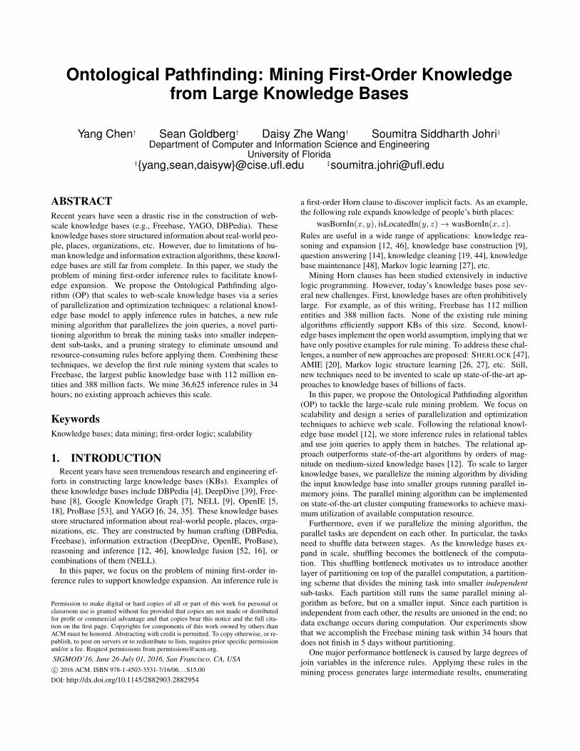
R1: Person1isMarriedTo−−−−−−→ Person2

livesIn−−−→ City livesIn←−−− Person1 isMarriedTo(P1, P2), livesIn(P2, C)→ livesIn(P1, C)

R2: Person directed−−−−→ Movie actedIn←−−−− Actor influences←−−−−− Person directed(P,M), actedIn(A,M)→ influences(P,A)

R3: Person worksAt−−−−→ Organization worksAt←−−−− Actor influences←−−−−− Person worksAt(P,O),worksAt(A,O)→ influences(P,A)

Figure 1: (Left) Cycles from Example 3. The first and last nodes in R1-R3 denote the same start and end node in the cycle. (Right)Corresponding rules.

4.3 Spark BasicsSpark is a cluster computing framework. Based on its core idea

of resilient distributed datasets (RDDs)–read-only collections ofobjects partitioned across a set of machines–it defines a set of par-allel operations. Using these operations, Spark allows users to ex-press a rich set of computation tasks. The operations we use in thispaper are listed below:• map/flatMap Transforms an RDD to a new RDD by applying

a function to each element in the input RDD.• groupByKey Transforms an RDD to a new RDD by grouping

by a user-specified key. In the result RDD, each key is mappedto a list of values of the key.• reduceByKey Transforms an RDD to a new RDD by grouping

by a user-specified key and performs a reduce function to thevalues of each key. In the result RDD, each key is mapped to theresult value of the reduce function.

In our parallel rule mining algorithm, we represent the set of facts{(s, p, o)} and the set of rules {(h, b1, b2)} as two RDDs and ex-press the algorithm using the above parallel operations.

5. ONTOLOGICAL PATHFINDINGThe Ontological Pathfinding (OP) algorithm is similar to rela-

tional pathfinding [42], but instead of finding paths over an entity-relationship graph, the OP algorithm searches the domain-rangeschema graph. The schema graph constrains the search space tosyntactically correct rules according to the arguments of each pred-icate. After constructing candidate rules, OP partitions them intosmaller independent parts. It accepts a maximum size argument s,a maximum rules size m, and partitions the candidate rules, mak-ing a best effort to satisfy the size requirements. Finally, OP prunescandidate rules with respect to the functional constraint t and eval-uates the rule batches using the parallel mining algorithm.

Algorithm 1 summarizes the major steps of Ontological Pathfind-ing to mine inference rules from a knowledge base Γ. We explaineach step in detail in the following sections.

Algorithm 1 Ontological Pathfinding(Γ, t, s,m)

1: M ← construct-rules(Γ.schema)2: {(Γi,Mi)} ← partition(Γ,∅,M, s,m)3: rules← ∅4: for all (Γi,Mi) do5: Mi ← prune(Γi, Mi, t)6: rules← rules ∪ parallel-rule-mining(Γi, Mi)7: return rules

5.1 Rule ConstructionAs discussed in Section 4.1, all entities and predicates are typed

in a knowledge base, i.e., each entity belongs to one or more types,and each predicate has a domain and a range. Typing restricts thepredicates that can be combined to form candidate rules: they musthave corresponding types for the joining variables. In this section,we utilize the schema to construct candidate rules.

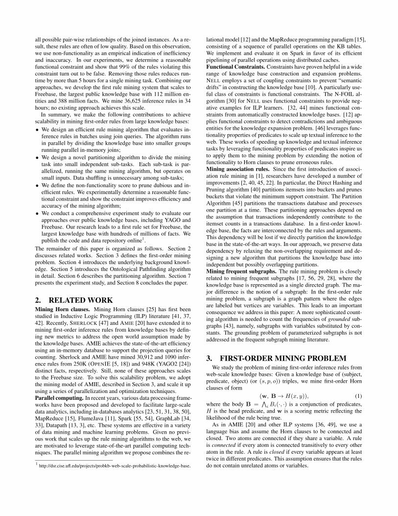
Definition 2. The schema graph of a knowledge base is definedto be a graph GΓ = (V,E), where V = {v1, . . . , v|V |} is theset of nodes representing types and E = {ep(vi, vj)} is the set oflabeled directed edges representing typed predicates p with vi asthe domain and vj as the range.

In a web-scale knowledge base like YAGO and DBPedia, we of-ten have a type hierarchy to divide types into subtypes for finer clas-sification. For instance, the “Person” type has subtypes including“Actor”, “Professor”. These types are related by the “subClassOf”edges. In Figure 2, we have a “subClassOf” edge from “Actor” to“Person”, indicating that “Actor” is a subtype of “Person”. To con-struct candidate rules, the subclasses need to inherit all the edgesfrom their ancestors. The inherited edges are defined in Defini-tion 3 using the following notations: 1. A(v) denotes the ancestornodes u of v such that there is a path from v to u with all edgeslabeled as “subClassOf”; and 2. E(u/v) denotes the neighboringnon-subClassOf edges of u with at least one u substituted by v.

Definition 3. We define the schema closure graph of a schemagraph G = (V,E) to be G′ = (V,E ∪ E′) where

E′ =⋃

v∈V,u∈A(v)

E(u/v).

Example 3. In Table 2, we provide an example schema from theYAGO knowledge base. Its schema graph is shown in Figure 2.In this graph, each type in the domain and range columns is repre-sented as a node, and each row in Table 2 is represented as an edgefrom domain to range. Since Actor is a subclass of Person, we inferadditional edges by having Actor inherit Person’s non-subClassOfedges, as shown by dashed arrows in Figure 2. �

Predicate Domain Range

livesIn Person CityisMarriedTo Person Person

worksAt Person Organizationdirected Person Movie

influences Person ActoractedIn Actor Movie

subClassOf Actor Person

Table 2: Example KB schema from YAGO knowledge base.

livesInPerson

Actor

City

Movie

Organization

isMarriedTo

directed

actedIn

subC

lass

Of

worksAt

influences

influences

worksAt

lives

In

**

* isMarriedTo

directed

isMarriedTo

Figure 2: Example schema closure graph. Dashed arrows indi-cate inherited edges.

R1

R2

R3

R1

R2

R3

Group joins CountGroup by facts

R1

R2

R3

F1F2, F5

F4

F2, F3F1

F2

F5F3, F4

F5

CheckGroup by join variables

Rules = {R1, R2, R3}

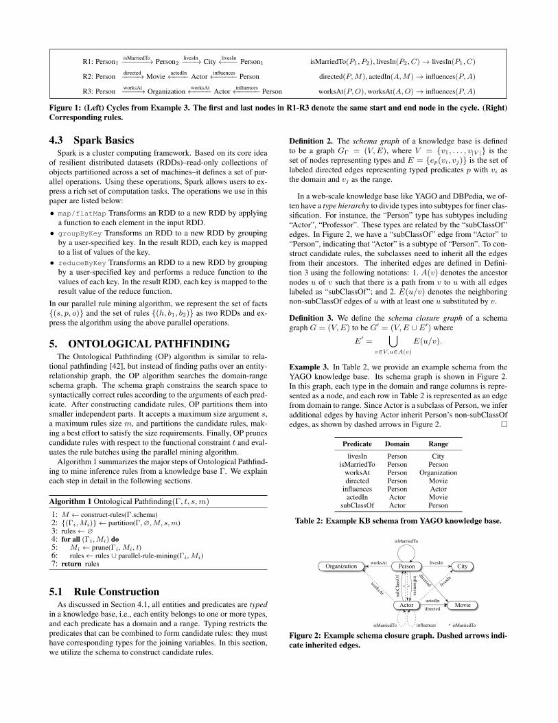
Figure 3: Parallel rule mining: KB divided into groups by join variables, each group running GROUP-JOIN to apply inference rules.

Following Definition 3, Algorithm 2 shows how to compute theclosure of a specific node v in a schema graph G by DFS. Whenvisiting a node v, we recursively visit its ancestors (Line 3) and addtheir neighboring edges to v (Line 4). Visiting each unvisited nodein G yields its schema closure graph.

Algorithm 2 Closure(G = (V,E), v)

1: if !v.visited then2: for all esubClassOf(v, u) ∈ E do3: Closure(G, u)4: E ← E ∪ E(u/v)5: v.visited← True

By traversing the closure graph, we identify a syntactically cor-rect rule when we detect a cycle. For instance, Figure 1 (Left)shows three example cycles from Example 3, and Figure 1 (Right)shows the corresponding rules constructed from the cycles. Al-though we have directed edges in the schema graph, we traverse itin an undirected manner: from any vertex v, we visit its neighborsfrom both incoming and outgoing edges. R3 shows an examplepath containing an inherited edge, Actor worksAt−−−−→ Organization, in-herited from Actor’s ancestor, Person.

5.2 Parallel Rule MiningGiven the relational knowledge base model in Section 4.2, we

store candidate inference rules in tables, allowing us to apply themin batches by joining the rules and facts tables. Furthermore, wedesign a parallel rule mining algorithm that divides the knowledgebase into groups running parallel in-memory group joins. We in-troduce the algorithm with the following equivalent class of rules:

p(x, y)← q(x, z), r(y, z).

In Section 5.2.1, we generalize it to other rule classes. We presentAlgorithm 3 using Spark primitives, but we note that it is a generalparallel algorithm consisting of basic parallel operations, conform-ing to the MapReduce paradigm. Figure 3 illustrates how Algo-rithm 3 transforms datasets using parallel operations.

In Step 1, we map each (s, p, o), i.e., (subject, predicate, ob-ject), triple to a pair (o, (p, s)), o serving as a key for the Group-ByKey operation that follows. In Step 2, the GroupByKey oper-ation groups all (o, (p, s)) tuples with the same object o into onegroup. This ensures the tuples with the same joining variable (o)are in the same group. In addition, we broadcast the rule table toeach group to ensure all relevant data are collocated for the joins.Consequently, the groups run disjoint in-memory group-joins, Al-gorithm 4, and are executed in parallel.

Algorithm 3 Parallel Rule MiningRequire: facts = {(pred, sub, obj)}Require: rules = {(ID, head, body1, body2)}1: Map each fact (pred, sub, obj) ∈ facts to (obj, (pred, sub)).2: GroupByKey obj, yielding a list of {(pred, sub)} pairs for each

obj.3: FlatMap the (obj, {(pred, sub)}) pairs to GROUP-JOIN(obj,

{(pred, sub)}, rules), using Algorithm 4, yielding a list of {(pred,sub, obj), rule.ID)} pairs.

4: ReduceByKey (pred, sub, obj), deduplicating the rule.ID s foreach (pred, sub, obj) triple.

5: FlatMap the ((pred, sub, obj), {rule.ID}) tuples toCHECK({rule.ID}), using Algorithm 5, yielding a list of {rID,(correct, 1)}pairs.

6: ReduceByKey rule.ID, summing the correct and 1 values.7: Map each (rule.ID, (sum, count)) to (rule.ID, sum/count)

pairs.

The GROUP-JOIN algorithm is an in-memory hash-join. Sincethe join variable o is matched by the previous GroupByKey, GROUP-JOIN matches predicates to the rule body. It starts by hashing theinput list of (p, s) pairs by predicate p (Line 3), creating a list ofsubjects for each p. This hash table is used to retrieve joined entitiesto be output as the subject and object as inferred by the rule. Foreach rule, its body predicates match two lists of subjects from thehash table. The algorithm infers the rule head with combinationsof subjects from the two matched lists (Lines 4-7).

In the GROUP-JOIN algorithm, we output the input facts (Line 2)and the inferred facts (Line 7). Each triple is output as a key, withthe value being the positive ID of the rule if it is inferred by thatrule, or 0 if it is from the input knowledge base. These IDs are usedto verify the inference results: if a fact is associated with an ID of0, it exists in the input knowledge base; otherwise, it is inferred byinference rules specified by the ID list.

Algorithm 4 GROUP-JOIN(obj, ps = {pred, sub}, rules)

1: for all (pred, sub) ∈ ps do2: emit ((pred, sub, obj), 0)3: preds← ps.groupBy(pred)4: for all r ∈ rules do5: for all sub1 ∈ preds.get (r.body1) do6: for all sub2 ∈ preds.get (r.body2) do7: emit ((r.head, sub1, sub2), r.ID)

In Step 4, we group by the output facts, each group computing alist of rule IDs that generate the fact. Algorithm 5 processes this listand determines if each rule is generating a correct fact by searching

for 0 in the list. It outputs a (ID, (c, 1)) tuple for each rule, where cindicates the correctness of the inferred fact. Thus, the component-wise sum of the (c, 1) tuples for each rule is the number of correctand total facts, respectively, inferred by the rule. Steps 6 and 7group by the rules, sum the correct and total counts, and computethe confidence of each rule.

Algorithm 5 CHECK(rs = {rule.ID})

1: correct← rs.contains(0)2: for all rule.ID ∈ rs do3: emit (rule.ID, (correct, 1))

The correctness of Algorithm 3 follows from the fact that theentire set of rules is broadcast to each group and that the groupsare disjoint from each other (recall that they are grouped by keyo). Therefore, Step 3 properly applies rules to the facts. In Step5, Algorithm 5 generates individual correct (0 or 1) and total (1)counts for rules inferring each fact. Since each fact contains the“0” flag to determine its correctness, aggregating the results fromall facts generates final correct and total counts for each rule.

5.2.1 General Rule MiningTo generalize Algorithm 3 to other rule classes, we recall from

Section 3 that the Horn clauses are assumed to be connected andclosed. Thus, for a general rule with rule ID r:

h(x, y)← b1, b2, . . . , bk,

we can arrange the body atoms so that each bi is connected to bi+1,i = 1, . . . , k − 1, and bk is connected to h(x, y), by a sharedvariable zi. The general rule mining algorithm, Algorithm 6, allowszi to be vectors and to contain repeated variables.

Algorithm 6 General Rule Mining

Require: facts = {(p, x, y)}Require: rules = {(r, h, b1, . . . , bk)}1: j1 ← facts2: for all pairs (bi, bi+1) with shared variable zi do3: ji ← ji.GroupByKey(zi)4: fi+1 ← facts.GroupByKey(zi)5: if i+ 1 < k then6: ji+1 ← {(zi+1, (r,xi+1))} =

GROUP-JOIN(ji, fi+1, rules)7: else8: jk ← {((h, x, y), r)} = GROUP-JOIN-LAST(ji, fk, rules)9: Process join result jk , as in Steps 4-7 of Algorithm 3.

Algorithm 6 joins two body atoms at a time. ji denotes the resultof joining b1, . . . , bi, and is used as the operand for joining the nextrule body, fi+1, in each iteration. The GROUP-JOIN and GROUP-JOIN-LAST methods in Lines 6 and 8 implement the rule seman-tics. GROUP-JOIN performs the join and outputs the tuples with thenext shared variable zi+1 as the key, along with the rule ID, r, andany variables referred to by the head or subsequent body atoms.GROUP-JOIN-LAST completes the join and infers facts from therules, generating a list of (fact, rule ID) pairs as in Algorithm 4 tobe further processed to evaluate the confidence of each rule, as inSteps 4-7 of Algorithm 3.

As a remark, we note that Algorithm 6 requires the input rulesbe of the same form. Thus, if there are N equivalent classes (de-fined in Section 4.2) of rules, we need N rule tables and N calls ofAlgorithm 6 to complete the mining task. On the other hand, eachrun of Algorithm 6 is highly efficient and optimized as we applythe rules in batches and in parallel. Thus, our approach trades offbetween generality and efficiency.

5.3 Rule PruningOne performance barrier we observe in the candidate rules is that

some of them generate prohibitively large intermediate results dueto large-degree variables in the joining predicates, as demonstratedby the following example:

diedIn(x, z),wasBornIn(y, z)→ hasAcademicAdvisor(x, y)(4)

In the above rule, we have variable z as the joining variable. Mean-while, in places with large populations, e.g., New York City, theCalifornia state, etc, there may be hundreds of thousands of peo-ple who were born or dead. Rules like this are untrustworthy, asmost of the intermediate results are irrelevant enumerations of theinvolving arguments (x, y in Rule (4)).

This large join problem is not uncommon among candidate rulesas they are constructed from the KB schema with no validation us-ing the facts. Thus, rules can accidentally have irrelevant predicatesthat coincide with the join variable with a large degree. To detectthese rules, we use histograms to determine the functional propertyof inference rules:• Predicate Histogram H0 = {(p, |{p(·, ·)}|)};• Predicate-Subject Histogram H1 = {(p, x, |{p(x, ·)}|)};• Predicate-Object Histogram H2 = {(p, y, |{p(·, y)}|)}.

In a functional notation, we writeH0(p) = |{p(·, ·)}|,H1(p, x) =|{p(x, ·)}|, and H2(p, y) = |{p(·, y)}|. H0 is used to computethe size of a KB partition, as explained in Section 6. H1 and H2

determine the size of intermediate results. For instance, the size ofthe join for Rule (4) can be computed by∑

z

H2(diedIn, z) ·H2(wasBornIn, z).

In the definition below, we omit the position descriptors (H1, H2)and use H(p, z) to denote the histogram entry for predicate p andjoin variable z in a general rule, the position of z determined by thejoin under consideration.

Definition 4. For a connected, closed rule r:

h← b1, . . . , bl,

we define the non-functionality of r as

NF(r) = maxbi,bj connected by z

{min(H(bi, z), H(bj , z))} . (5)

A functional constraint t accepts rules r with NF(r) ≤ t.

According to Definition 4, a functional constraint requires eachjoin, represented by a pair of connected atoms of the rule, have ajoin variable z with no more than t joined instances as determinedby min(H(bi, z), H(bj , z)), z ranging over all joined values. Weuse non-functionality as an empirical indication of rule correctness.Viewing a knowledge graph as a sparse natural graph–e.g., Free-base and YAGO2s has a sparsity of 3.11× 10−8 and 9.82× 10−7,respectively–we justify our approach by the empirical power-lawdegree distribution of natural graphs that only a few entities in aknowledge graph have a large degree [21], implying that neighborsof large degree entities are unlikely inter-connected with one an-other as suggested by the non-functional joins.

In our experiment, we observe that violations of functional con-straints are strong indications of incorrectness of the rules, andmore than 99% of the non-functional rules are wrong. Removingthose erroneous rules improves performance and rule quality. Byvarying the constraint t, we show that a reasonable choice lies be-tween 50 and 250 and set t = 100 in the default configuration. Weexperimentally justify our choice in Section 7.4.

Output 1

Output 2

Output 3

Output

Independent Overlapping Partitions

Partition 1

Partition 2

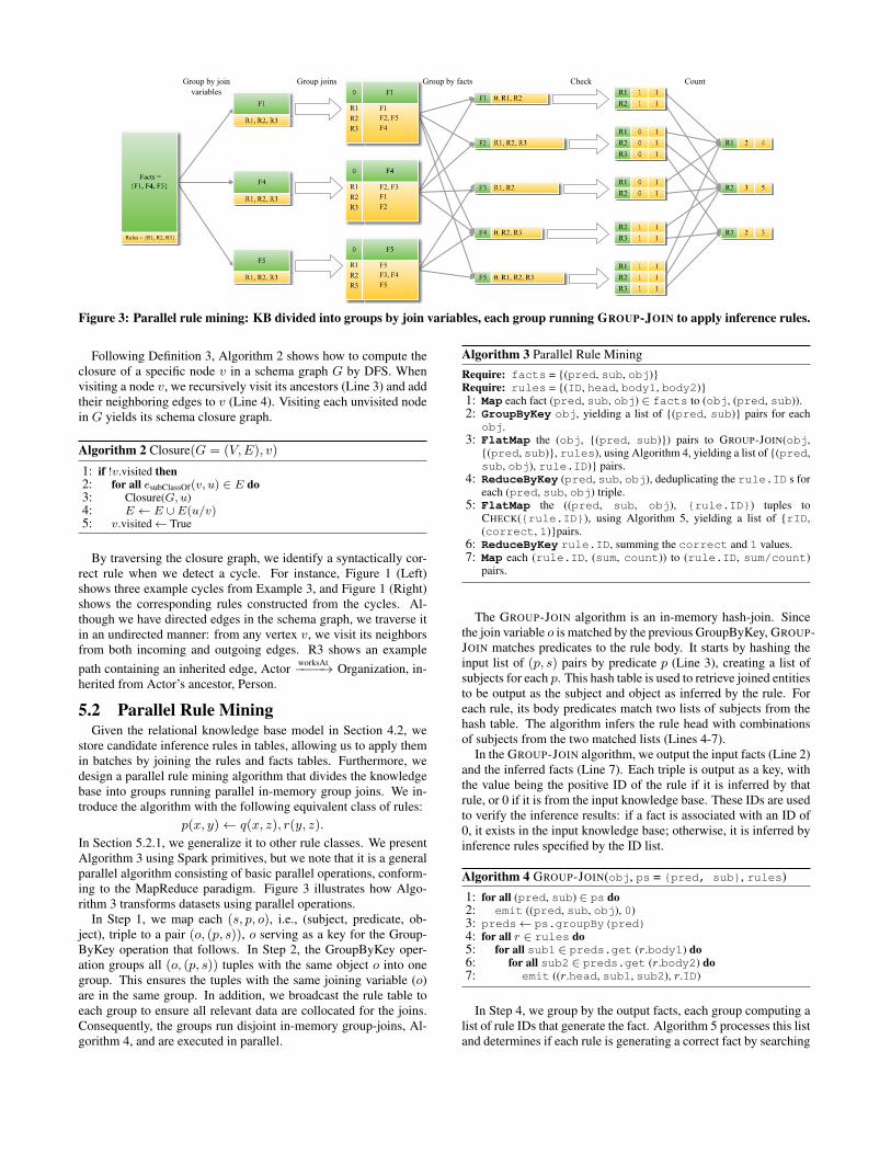
Figure 4: Partitioning algorithm: KB partitioned into smaller overlapping parts running independent mining algorithm instances.

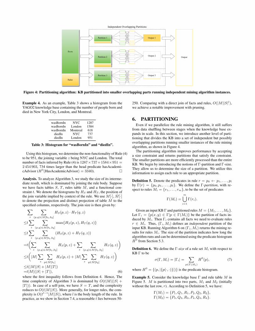
Example 4. As an example, Table 3 shows a histogram from theYAGO2 knowledge base containing the number of people born anddied in New York City, London, and Montreal.

wasBornIn NYC 1287wasBornIn London 1584wasBornIn Montreal 618

diedIn NYC 737diedIn London 951

Table 3: Histogram for “wasBornIn” and “diedIn”.

Using this histogram, we determine the non-functionality of Rule (4)to be 951, the joining variable z being NYC and London. The totalnumber of facts inferred by Rule (4) is 1287×737+1584×951 =2 454 903, 734 times larger than the head predicate hasAcademi-cAdvisor (H0(HasAcademicAdvisor) = 3340). �

Analysis. To analyze Algorithm 3, we study the size of its interme-diate result, which is dominated by joining the rule body. Supposewe have facts tables S, T , rules table M , and a functional con-straint t. We denote the histograms by HS and HT , the position ofthe join variable implied by context of the rule. We use M [·], M [·]to denote the projection and distinct projection of table M to thespecified columns, respectively. The join size is then given by:∑

z

∑(p,q)∈M [b1,b2]

HS(p, z) ·HT (q, z)

≤t∑z

∑(p,q)∈M [b1,b2]

max{HS(p, z), HT (q, z)}

≤t∑z

∑(p,q)∈M [b1,b2]

(HS(p, z) +HT (q, z))

=t

(∑z

∑(p,q)∈M [b1,b2]

HS(p, z) +∑z

∑(p,q)∈M [b1,b2]

HT (q, z)

)≤t(|M |

∑z

∑p∈M [b1]

HS(p, z) + |M |∑z

∑q∈M [b2]

HT (q, z)

)≤t(|M ||S|+ |M ||T |)=t|M |(|S|+ |T |), (6)

where the first inequality follows from Definition 4. Hence, Thetime complexity of Algorithm 3 is dominated by O(t|M |(|S| +|T |)). In case of a self-join, we have S = T , and the complexityreduces to O(t|M ||S|). More generally, for longer rules, the com-plexity is O(tl−1|M ||S|), where l is the body length of the rule. Inpractice, as we show in Section 7.4, a reasonable t lies between 50-

250. Comparing with a direct join of facts and rules, O(|M ||S|l),we achieve a notable improvement with pruning.

6. PARTITIONINGEven if we parallelize the rule mining algorithm, it still suffers

from data shuffling between stages when the knowledge base ex-pands in scale. In this section, we introduce another level of parti-tioning that divides the KB into a set of independent but possiblyoverlapping partitions running smaller instances of the rule miningalgorithm, as shown in Figure 4.

The partitioning algorithm improves performance by acceptinga size constraint and returns partitions that satisfy the constraint.The smaller partitions are more efficiently processed than the entireKB. We begin by introducing the notions of Γ-partition and Γ-size.They allow us to determine the size of a partition. We utilize thisinformation to assign each rule to an appropriate partition.

Definition 5. Denote the predicates in rule r = p0 ← p1, . . . , plby Γ(r) = {p0, p1, . . . , pl}. We define the Γ-partition, with re-spect to rules Mi = {r1, . . . , rm}, to be the set of predicates

Γ(Mi) =

m⋃i=1

Γ(ri).

Given an input KB Γ and partitioned rulesM = {M1, . . . ,Mk}.Let Γi = {p(x, y) ∈ Γ|p ∈ Γ(Mi)} be the partition of facts in-duced by Mi. Then Γi contains all facts we need to evaluate rulesr ∈ Mi. Thus, (Γi,Mi) defines an independent partition of theinput KB. Running Algorithm 6 on (Γi,Mi) returns the mining re-sults for rules Mi. The size of the partition indicates how long thealgorithm runs and can be determined using the predicate histogramH0 from Section 5.3.

Definition 6. We define the Γ-size of a rule set Mi with respect toKB Γ to be

σ(Γ,Mi) = |Γi| =∑

p∈Γ(Mi)

H0(p), (7)

where H0 = {(p, |{p(·, ·)}|)} is the predicate histogram.

Example 5. Consider the knowledge base Γ and rule table M inFigure 5. M is partitioned into two parts, M1 and M2 (initiallywithout the last row, r). According to Definition 5, we have:

Γ(M1) = {P1, Q1, R1, P2, Q2, R2},Γ(M2) = {P3, Q3, R3, P4, Q4, R4}.

h b1P1 Q1P2 Q2

b2R1R2

P3 Q3P4 Q4

R3R4

P2 Q3 R4

M1

M2

r

M

Figure 5: Rule table M , initial partitions M1, M2, and unpar-titioned rule r.

Assuming each predicate has 1 fact, namely,H0(Pi) = H0(Qi) =H0(Ri) = 1, we have σ(Γ,M1) = σ(Γ,M2) = 6.Now consider the addition of rule r = (P2, Q3, R4). We have:

Γ(M1 ∪ {r}) = {P1, Q1, R1, P2, Q2, R2, Q3, R4},Γ(M2 ∪ {r}) = {P3, Q3, R3, P4, Q4, R4, P2}.

Consequently, σ(Γ,M1∪{r}) = 8, σ(Γ,M2∪{r}) = 7. Addingr to M2 incurs a smaller increase of size than adding it to M1. �

Given an upper bound of the Γ-size s and the number of rules mfor each partition, our goal is to find a partition {M1, . . . ,Mk} ofM that satisfies the following constraints:

(C1) σ(Γ,Mi) ≤ s, 1 ≤ i ≤ k(C2) |Mi| ≤ m, 1 ≤ i ≤ k

(C3)k⋃

i=1

Mi = M,

(C4) Mi ∩Mj = ∅, 1 ≤ i < j ≤ kWe seek to find a partition {M1, . . . ,Mk} with as a small k as

possible. Without a priori knowledge of the optimal k, we use arecursive binary partitioning scheme in Algorithm 7. In each re-cursive step, the input rule set M is partitioned into two smallerparts, M1 and M2. The algorithm terminates when all partitionssatisfy the size constraints (C1) and (C2). The partitions satisfy thecompleteness and disjointness constraints (C3) and (C4) at each re-cursive step as M is partitioned into M1 and M2 by Algorithm 8such that M1 ∪M2 = M and M1 ∩M2 = ∅.

Algorithm 7 RecPartition(Γ,Π,M, s,m)

1: if σ(Γ,M) ≤ s and |M | ≤ m then2: Π← Π ∪ {M}3: else4: (M1,M2)← 2-Partition(Γ,M)5: if M1 = ∅ then6: Π← Π ∪ {M2}7: else if M2 = ∅ then8: Π← Π ∪ {M1}9: else

10: RecPartition(Γ,Π,M1, s,m)11: RecPartition(Γ,Π,M2, s,m)

Specifically, we first determine whether to partition the input Mby checking if it already satisfies the size constraints (C1) and (C2)(Line 1). If it does, we add it to the final set of partitions and re-turn (Line 2); otherwise, we use a binary partitioning algorithm topartition the rules (Line 4) and recursively partition the sub-parts(Lines 10-11). Lines 5-8 handle special cases where the size con-straint (C1) cannot be satisfied. This happens when s < H0(p) forsome predicate p. The binary partitioning algorithm is describedin Algorithm 8, using a greedy assignment strategy: each rule isassigned to the partition with a smaller increase in size (Lines 4-9).Note that in Lines 4-5, we add a penalty term p(Γ,M) to penal-ize the larger partition, preventing it from absorbing all subsequent

Algorithm 8 2-Partition(Γ,M)

1: M1 ← ∅2: M2 ← ∅3: for all r ∈M do4: ∆1 ← σ(Γ,M1 ∪ {r})− σ(Γ,M1) + p(Γ,M1)5: ∆2 ← σ(Γ,M2 ∪ {r})− σ(Γ,M2) + p(Γ,M2)6: if ∆1 < ∆2 then7: M1 ←M1 ∪ {r}8: else9: M2 ←M2 ∪ {r}

10: return (M1,M2)

rules, as duplicate predicates do not increase the partition size. Inour experiments, we set p(Γ,M) = 1

50σ(Γ,M).

Analasis. Algorithm 7 makes a best effort to satisfy the size re-quirement s. If H0(p) > s for some predicate p, Algorithm 7returns in Lines 5-8 without partitioning the predicate. AssumingAlgorithm 7 results in N partitions {M1, . . . ,MN}, the size ofthe largest partition being sm, then the overall time complexity toevaluate the partitioned facts and rules tables, based on (6), is:N∑i=1

O(tl−1sm|Mi|) = O

(tl−1sm

N∑i=1

|Mi|

)= O(tl−1sm|M |),

(8)where t is the functional constraint and l is the length of the rulebody as in Section 5.3. The time complexity is bounded with re-spect to the largest partition instead of the input knowledge base.Thus, partitioning reduces time complexity from O(tl−1|Γ||M |)to O(tl−1sm|M |), allowing us to control the complexity by tuningthe size constraints for very large knowledge bases.

Since Γ-partitions are induced from partitions of inference rules(Definition 5) and rules from different partitions may contain du-plicate head or body predicates, the Γ-partitions may overlap, asillustrated by the addition of rule r in Example 5. To measure thisoverlap, we introduce the notion of degree of overlap.

Definition 7. The degree of overlap (DOV) of a set of rule partsM = {M1,M2, . . . ,Mk} is defined to be

DOV(M) =

∑i σ(Γ,Mi)

σ(Γ,⋃

i Γ(Mi)) . (9)

In Equation (9), the numerator∑

i σ(Γ,Mi) is the total size ofthe partitions we make to evaluate the inference rules. The denom-inator σ

(Γ,⋃

i Γ(Mi))

is the size of the KB induced by rules M .A DOV greater than 1 indicates overlapping partitions.

Example 6. Consider the partitioning scheme from Example 5.While the initial partitions M1 and M2 are disjoint, adding r toM1 or M2 results in overlapping partitions:

DOV({M1,M2}) =6 + 6

12= 1;

DOV({M1,M2 ∪ {r}}) =6 + 7

12= 1.0833;

DOV({M1 ∪ {r},M2}) =8 + 6

12= 1.1667. �

Partition Independence. We conclude this section by remarkingthe difference between partitioning in Algorithm 7 and paralleliza-tion in Algorithm 3. Algorithm 7 breaks the input knowledge baseinto smaller independent partitions so that each partition runs itsown instance of Algorithm 3. Algorithm 3 divides the input knowl-edge base into correlated groups running sub-procedures of a sin-

gle mining task. Algorithm 3 is used by Algorithm 7 as the paral-lel mining algorithm in each partition. The two-level partitioning-parallelization scheme is elucidated in Figure 4. These techniquescombined scale the rule mining algorithm to Freebase.

7. EXPERIMENTSWe validate our approaches by mining inference rules from YAGO

and Freebase. Our work contributes the first rule set for Freebase–36,625 first-order inference rules. In this section, we present our re-sults, compare with the state-of-the-art KB rule mining algorithm,AMIE [21], and analyze individual techniques from Sections 5and 6. We begin by describing the datasets and experiment setup.YAGO. YAGO is a knowledge base derived from Wikipedia, Word-Net, and GeoNames. Its newest version, YAGO2s, has more than10M entities and 120M facts, including the schema, taxonomy, corefacts, etc. We use the schema for rule construction and the core4.48M binary facts for rule evaluation.Freebase. Freebase is a community-curated knowledge base ofwell-known people, places, and things, containing 112M entitiesand 2.68B facts, as of current writing. We preprocess the dataset byremoving the multi-language support and use the remaining 388Mfacts. The datasets statistics are summarized in Table 4 (Left).

KB Size

YAGO2 # Entities = 834,554# Facts = 948,047

YAGO2s # Entities = 2,137,468# Facts = 4,484,907

Freebase # Entities = 111,781,246# Facts = 388,474,630

Max length 3

Max Γ-size 3M (YAGO)10M (Freebase)

Max # of rules 1000Functionalconstraint

100

Min support 0Min confidence 0.0

Table 4: (Left) Datasets statistics. (Right) Default parameters.

Experiment setup. We conduct all experiments on a 64-core ma-chine running on AMD Opteron processors at 1.4GHz, with 512GBRAM and 3.1TB disk space. The OP and AMIE algorithms are im-plemented in Spark and Java/SQL, respectively, running on Spark1.3.0, Java 1.8, and PostgreSQL 9.2.3.Default parameters. Unless otherwise specified or the current pa-rameter is under evaluation, we use the default parameters in Ta-ble 4 (Right) for the experiments. We determine the parameters bytrying multiple parameter combinations and comparing the perfor-mance and result rules. For Freebase experiments in Sections 7.2to 7.4, we report the result of one class of length 3 rules.Rule set precision. We evaluate a rule set by assessing its mostconfident rules, i.e., with a minimum confidence of 0.6 and support-ing at least 2 facts. Under this constraint, we define the precisionof a rule set as the percentage of rules satisfying the above thresh-old that we consider correct. Each rule is rated by two independenthuman judges. In case of a disagreement, the judges conduct a de-tailed discussion until a final decision is made. We sample at most300 rules from each rule set for human inspection.

7.1 Overall ResultTo evaluate performance of the OP algorithm and compare with

the state-of-the-art, we run the OP and AMIE algorithms on Free-base and YAGO. As a result, OP mines 36,625 rules in 33.22 hoursfrom Freebase, contributing the largest first-order rules repositorycreated from public knowledge bases. We compare the detail per-formance metrics, including the number and precision of minedrules, and the runtime for each knowledge base, in Table 5.

In terms of efficiency and scalability, OP outperforms AMIE inall the experiments we run. For Freebase, AMIE takes more than

Dataset Algorithm # Rules Precision Runtime

YAGO2 OP 218 0.35 3.59 minAMIE 1090 0.46 4.56 min

YAGO2s OP 312 0.35 19.40 minAMIE 278+ N/A 5+ d

Freebase OP 36,625 0.60 33.22 hAMIE 0+ N/A 5+ d

Table 5: Overall mining result.

5 days to generate a single rule (AMIE outputs an inference ruleonce it has determined its quality), whereas OP finishes in 33.22hours. For the smaller YAGO2s KB, AMIE mines 278 rules in 5days while OP mines 312 rules in 19.40 minutes. For YAGO2, dueto its small size, partitioning and parallelization have limited ad-vantage, so OP is only 0.97 minutes faster. The quantity of minedrules is large: 36,625 first-order rules from Freebase, spanning avariety of topics: film, book, music, computer, etc, as shown in Fig-ures 6 and 11(3). OP mines fewer rules from YAGO2 and YAGO2sbecause their sizes are much smaller, and their schemas are incom-plete. Possible domain and range values are missing from over-loaded predicates, so the rule construction algorithm generates asubset of all possible rules from the available schema. Using amore accurate schema, e.g., the Freebase schema, improves recall.

In terms of precision, Freebase rules achieve 0.60, outperform-ing YAGO rules by more than 0.1. The precision benefits fromFreebase’s cleaner data and schema. To illustrate, consider Rule(1) in Figure 6 with predicates “film/film/sequel” and “film/film/-country”. These predicates impose precise constraints on the data:“sequel” refers to the sequel of a film, and “country” refers to theproducing country of a film. Such constraints ensure that Freebasepredicates contain fine-grained and accurate data instances. On theother hand, because 1) YAGO has fewer predicates, and 2) YAGOpredicates are less well-defined, YAGO generates fewer rules withlower quality. Consider the “create” predicate from YAGO2s: thedomain is possibly writer, musician, filmmaker, author, etc, andthe range can be book, music, film, novel, etc. Thus, “create” canbe combined with any matching predicates to form candidate rules,leading to spurious results. The rule “created(x, z), created(y, z)→isMarriedTo(x, y)” illustrates this situation. Other predicates, like“playsFor”, “owns”, “influences”, are similarly misused.

Figures 7(a)(b) report OP’s performance for one class of rules ofeach length from 2 to 5. We mine 1,006 and 83,163 for YAGO2s(lengths 4 and 5) and Freebase (length 4) in 8.62 and 82.77 hours,respectively. For rule construction, because the schema is muchsmaller than the knowledge base, it takes 13.64 and 0.94 minutesfor YAGO2s and Freebase, accounting for less than 3% of the run-time. The construction process for YAGO2s is slower than forFreebase since its predicates are heavily overloaded, as we discussabove, resulting in expensive joins, especially for long rules.

Analyzing the rules, we observe that 90.3% of them reduce tolengths 2 and 3 rules, as shown in Figure 7(c). We classify theserules as trivial extensions and composite rules. We call a rule triv-ial extension of another rule if it can be reduced to the other ruleby applying and removing any valid rules from its body. In Fig-ure 6, Rule (4) is a trivial extension of Rule (3) since the rulebook/book/first_edition(x, u)→ book/book_edition/book(u, x) in-fers that v = x in (4). By replacing v with x and removing theapplied rule, it reduces to (3). We call a rule composite if it can berewritten by chaining shorter rules. For instance, Rule (5) in Fig-ure 6 is a composite rule of (1) and (2). Rule (6) gives an exampleof correct and irreducible length 4 rule.

Confidence Rule(1) 0.81 film/film/sequel(x, z), film/film/country(z, y)→ film/film/country(x, y)(2) 0.44 film/film/country(x, z), location/country/official_language(z, y)→ film/film/language(x, y)(3) 1.0 book/book/first_edition(x, y)→ book/book/editions(x, y)(4) 1.0 book/book/first_edition(x, u), book/book_edition/book(u, v), book/book/first_edition(v, y)→ book/book/editions(x, y)(5) 0.41 film/film/sequel(x, u), film/film/country(u, v), location/country/official_language(v, y)→ film/film/language(x, y)(6) 0.89 music/music_video/music_video_song(x, u), music/composition/recorded_as_album(u, v), music/album/artist(v, y)→

music/music_video/artist(x, y)

Figure 6: Example Freebase rules.

2 3 4 5Rule Length

0

100

200

300

400

500

600

700

# M

ined

Rul

es

0.0

0.2

0.4

0.6

0.8

1.0

Prec

isio

n

# RulesPrecisionRuntime

0

1

2

3

4

5

6

7

8

Run

time/

h

(a) YAGO2s General Rules

2 3 4Rule Length

0100002000030000400005000060000700008000090000

# M

ined

Rul

es

0.0

0.2

0.4

0.6

0.8

1.0

Prec

isio

n

# RulesPrecisionRuntime

0

20

40

60

80

100

Run

time/

h

(b) Freebase General Rules

Correct3.4%

Incorrect6.3%

Composite

9.0%

Trivialextensions

81.3%

(c) Freebase Length 4 Rules

Figure 7: (a)(b) OP performance for mining lengths 4 (YAGO and Freebase) and 5 (YAGO) rules.(c) Quality of Freebase length 4 rules.

0 10 20 30 40 50 60# Cores

1

2

3

4

5

Spee

dup

Effect of Parallelism

YAGO2s speedupYAGO2s database runtimeFreebase speedup

Figure 8: Effect of paral-lelism.

The trivial extensions and composite rules provide little knowl-edge in addition to lengths 2 and 3 rules. Thus, their distributionin Figure 7(c) implies limited benefits from mining longer rules.We remove those rules and evaluate the remaining rules as we dowith length 2 and 3 rules. As a result, the precision is much lowerthan the lengths 2 and 3 rules: 0.04 for YAGO2s and 0.03 for Free-base, as reported in Figure 7. These results suggest the primary andfoundational importance of shorter rules in a knowledge base. Wetherefore limit the maximum length to 3 in the default setting.

In summary, the overall results justify the benefits of OP algo-rithm to mine web-scale knowledge bases. In the remainder of thissection, we examine individual techniques of parallelism, partition-ing, and rule pruning in greater details and show how they improvethe performance and quality of the rule mining task.

7.2 Effect of ParallelismWe evaluate the effect of parallelism by comparing the parallel

mining algorithm with a SQL implementation on PostgreSQL. Wevary the number of cores for parallel mining from 1 to 64 and reportin Figure 8 the relative speedup compared to running on 1 core. Asa result, the parallel mining algorithm achieves a speedup of 5.70and 3.34 on YAGO2s and Freebase, respectively. Comparing withthe SQL approach, parallel mining achieves a speedup of 3.16 onYAGO2s and a much higher speedup on Freebase–the SQL queriesdo not scale to Freebase in the experiments on PostgreSQL and onan in-house parallel database system, Datapath [3]. The speedupresults from 1) the SQL query performs one large join while Algo-rithm 3 runs smaller joins in parallel; 2) the shuffling step in Sparkis more efficient than the deduplication operation in PostgresSQLgiven a large output from previous joins.

These results attest to the overall advantage of parallelizing therule mining algorithm. Nonetheless, we see the parallelization doesnot make full use of available 64 processors, because the outputsizes and performance of GROUP-JOINs vary greatly among groups,depending on the data distribution, and is dominated by the slowestjoins among the groups. Moreover, the efficiency of the shufflingstep is restricted by data dependency among parallel workers.

7.3 Effect of PartitioningPartitioning is a key step in scaling up the mining algorithm. By

setting a maximum Γ-size s and number of rulesm, the partitioningalgorithm breaks the input knowledge base into parts with no larger

than the specified size. Our experiments show the OP algorithmcompletes the Freebase mining task in 1.39 days with partitioning,which otherwise takes more than 5 days with no success.

The result of Freebase partitioning is illustrated in Figure 9: inthe left figure, we set s = 20M and m = 2K; in the right figure,we set s = 200M and m = 10K. For the former case, we have65 partitions, all running faster than partitions from the latter case,with the fastest partition finishing in 14.18 seconds and the slowestin 1.17 hours. For the latter case, we have 5 large partitions, thefastest taking 4.58 hours to finish and the slowest taking 1.27 days.

The effect of choosing different partition sizes is shown in Fig-ures 10(a)-(c) for Freebase and Figure 10(d) for YAGO2s. In theFreebase experiments, the effect of partitioning is substantial: aswe vary s from 200M to 5M and m from 10K to 1K, the total run-time decreases from 2.55 days to 5.06 hours. The reason for suchspeedup is because the partitioning algorithm manages to split theinput knowledge base into smaller ones that are more efficientlyjoined, and the overhead of the overlap is less significant as thebenefit from joining smaller tables. This benefit can be further ver-ified by the decline of runtime of the largest partitions from 1.27days to 38.14 minutes as we lower the size constraints, as shownin Figure 10(b), indicating that the partitions are more efficientlyjoined because of their smaller sizes. Consequently, the overallruntime significantly drops despite partition overlaps.

In Figure 10(c), we show the DOV increases from 1.14 to 1.35as we create smaller partitions. The increasing DOV means wespend more time partitioning Freebase: from 2.45 minutes to 61.43minutes. Comparing with Figure 10(a), we see the reduction fromjoining smaller partitions has greater impact on the total runtime.

On the other hand, if s and m become too small, the overhead ofoverlapping partitions begins to dominate. The overlapping effectis shown in Figure 10(d) as we partition the 4.48M YAGO2s intosmaller parts: while we improve the runtime of the slowest partitionfrom 5.80 minutes to 1.79 minutes, the total runtime rises to 29.60minutes after hitting the optimum of 19.40 minutes when s = 3Mand m = 500. The fall of performance is caused by the growingnumber of overlapping partitions. The extreme case of applyingone rule at a time, taken by state-of-the-art approaches, is equiva-lent to having one rule in each partition. Given a large search spaceof candidate rules, it implies a large number of queries, hence toomuch overlapping overhead for it to be efficient.

Partitions0

5

10

15

20

25

30Pa

rtitio

n si

ze £

rule

size

/109

Freebase Partitions (s=20M, m=2K)

0

10

20

30

40

50

60

70

80

Run

time/

min

Partition size £ rule sizeRuntime

Partitions0

100

200

300

400

500

600

700

Parti

tion

size

£ ru

le si

ze/109

Freebase Partitions (s=200M, m=10K)

200

400

600

800

1000

1200

1400

1600

1800

2000

Run

time/

min

Partition size £ rule sizeRuntime

Figure 9: Sizes and runtime of Freebase partitions.

050100150200Max Partition size/M

10

20

30

40

50

60

Run

time/

h

m = 10K

m = 5K

m = 2K

m = 1K

(a) Freebase: Runtime vs Partitioning

050100150200Max Partition size/M

0

5

10

15

20

25

30

Run

time/

h

m = 10K

m = 5K

m = 2K

m = 1K

(b) Freebase: Max Runtime vs Partitioning

050100150200Max Partition size/M

1.00

1.05

1.10

1.15

1.20

1.25

1.30

1.35D

OV

m = 10K

m = 5K

m = 2K

m = 1K(c) Freebase: DOV vs Partitioning

01234Max Partition size/M

5

10

15

20

25

30

Run

time/

min

m = 1000

m = 500

m = 1000; max runtime m = 500;max runtime

(d) YAGO2s: Runtime vs Partitioning

0 100 200 300 400 500 600Functional Constraint

01020304050607080

YA

GO

2s R

untim

e/m

in

0

2

4

6

8

10

12

14

Free

base

Run

time/

h

(e) Runtime vs Functional Constraint

YAGO2s runtimeFreebase runtime

0 100 200 300 400 500 600Functional Constraint

0.80

0.85

0.90

0.95

1.00

Prun

ing

Prec

isio

n1000

2000

3000

4000

5000

6000

# Pr

uned

Rul

es

(f) Pruned Rules Quality

YAGO2s pruning precisionYAGO2s # pruned rulesFreebase pruning precisionFreebase # pruned rules

Figure 10: (a)-(d) Runtime by varying partition sizes. (e)-(f) Runtime and accuracy by varying functional constraints.

7.4 Effect of Rule PruningThe functional constraint t affects the mining algorithm in terms

of both performance and quality. To evaluate the accuracy, we de-fine the pruning precision of pruned rules as the percentage of thoserules that we consider erroneous. Thus, a high pruning precisionindicates that erroneous rules are pruned as desired and justifiesthe proposed approach. As we vary the functional constraint t andprune violating rules, we report the runtime, number and pruningprecision of pruned rules in Figures 10(e)(f).

We make two observations from Figures 10(e)(f): (1) When t ≥200, the pruning precision reaches its maximum value of 1.0–allpruned rules are erroneous. However, the runtime grows from 9.55hours to 14.27 hours, indicating wasted computation in evaluat-ing wrong rules that should otherwise be eliminated by setting asmaller t. (2) On the other hand, decreasing t from 50 to 2 causesthe pruning precision to drop sharply from 0.995 to 0.82 while im-proving runtime only by 1.54 hours from 7.97 to 6.43 hours.

From the above observations, we see the rule pruning process im-proves both performance and quality provided we choose a propert constraint. Based on Figure 10(f), a value between 50 and 250is reasonable. In our default setting, we have t = 100 and de-tect 101 and 2352 non-functional rules from YAGO2s and Free-base, respectively. For Freebase, more than 99% rules are cor-rectly pruned. Rules (1) and (2) from Freebase in Figure 11 il-lustrate the common reason why functional constraints are vio-lated: in Freebase and other knowledge bases, we have many-one,

many-few, and many-many predicates. The “location/location/con-tainedBy” predicate in Rule (1), for example, is a many-few pred-icate. The rule construction algorithm, based on the KB schema,is unaware of the functionality properties of the predicates. Whenthe one or few variable happens to be the join variable, the rule vi-olates the functional constraint. Rule (3) is an incorrectly prunedrule due to a low t = 5 functional constraint. The “computer/-computer_processor/variants” predicate defines an equivalence re-lation: variants of a computer processor are variants of each other.According to the sparsity of natural graphs [21], we reduce pruningerrors by raising the functional constraint t.

8. CONCLUSIONIn this paper, we address the scalable first-order rule mining

problem. We present the Ontological Pathfinding algorithm to minefirst-order inference rules from web-scale knowledge bases. Weachieve the Freebase scale via a series of parallelization and opti-mization techniques: a relational knowledge base model that ap-plies inference rules in batches, a rule mining algorithm that par-allelizes the join queries, a novel partitioning algorithm that di-vides the mining task into smaller independent sub-tasks, and arule pruning strategy to detect incorrect and resource-consumingrules. Combining these techniques, we mine the first rule set forFreebase, the largest public knowledge base with 388 million factsand 112 million entities, in 34 hours. No existing system achievesthis scale. We publish our code and data repositories online.

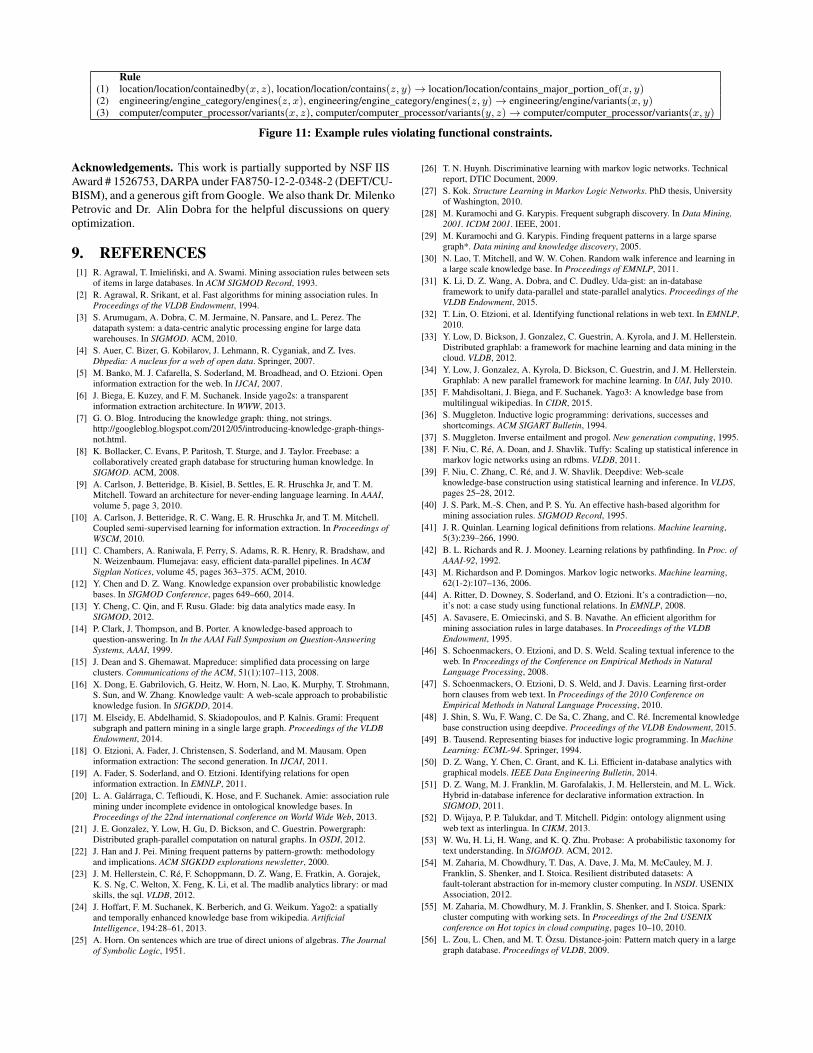
Rule(1) location/location/containedby(x, z), location/location/contains(z, y)→ location/location/contains_major_portion_of(x, y)(2) engineering/engine_category/engines(z, x), engineering/engine_category/engines(z, y)→ engineering/engine/variants(x, y)(3) computer/computer_processor/variants(x, z), computer/computer_processor/variants(y, z)→ computer/computer_processor/variants(x, y)

Figure 11: Example rules violating functional constraints.

Acknowledgements. This work is partially supported by NSF IISAward # 1526753, DARPA under FA8750-12-2-0348-2 (DEFT/CU-BISM), and a generous gift from Google. We also thank Dr. MilenkoPetrovic and Dr. Alin Dobra for the helpful discussions on queryoptimization.

9. REFERENCES[1] R. Agrawal, T. Imielinski, and A. Swami. Mining association rules between sets

of items in large databases. In ACM SIGMOD Record, 1993.[2] R. Agrawal, R. Srikant, et al. Fast algorithms for mining association rules. In

Proceedings of the VLDB Endowment, 1994.[3] S. Arumugam, A. Dobra, C. M. Jermaine, N. Pansare, and L. Perez. The

datapath system: a data-centric analytic processing engine for large datawarehouses. In SIGMOD. ACM, 2010.

[4] S. Auer, C. Bizer, G. Kobilarov, J. Lehmann, R. Cyganiak, and Z. Ives.Dbpedia: A nucleus for a web of open data. Springer, 2007.

[5] M. Banko, M. J. Cafarella, S. Soderland, M. Broadhead, and O. Etzioni. Openinformation extraction for the web. In IJCAI, 2007.

[6] J. Biega, E. Kuzey, and F. M. Suchanek. Inside yago2s: a transparentinformation extraction architecture. In WWW, 2013.

[7] G. O. Blog. Introducing the knowledge graph: thing, not strings.http://googleblog.blogspot.com/2012/05/introducing-knowledge-graph-things-not.html.

[8] K. Bollacker, C. Evans, P. Paritosh, T. Sturge, and J. Taylor. Freebase: acollaboratively created graph database for structuring human knowledge. InSIGMOD. ACM, 2008.

[9] A. Carlson, J. Betteridge, B. Kisiel, B. Settles, E. R. Hruschka Jr, and T. M.Mitchell. Toward an architecture for never-ending language learning. In AAAI,volume 5, page 3, 2010.

[10] A. Carlson, J. Betteridge, R. C. Wang, E. R. Hruschka Jr, and T. M. Mitchell.Coupled semi-supervised learning for information extraction. In Proceedings ofWSCM, 2010.

[11] C. Chambers, A. Raniwala, F. Perry, S. Adams, R. R. Henry, R. Bradshaw, andN. Weizenbaum. Flumejava: easy, efficient data-parallel pipelines. In ACMSigplan Notices, volume 45, pages 363–375. ACM, 2010.

[12] Y. Chen and D. Z. Wang. Knowledge expansion over probabilistic knowledgebases. In SIGMOD Conference, pages 649–660, 2014.

[13] Y. Cheng, C. Qin, and F. Rusu. Glade: big data analytics made easy. InSIGMOD, 2012.

[14] P. Clark, J. Thompson, and B. Porter. A knowledge-based approach toquestion-answering. In In the AAAI Fall Symposium on Question-AnsweringSystems, AAAI, 1999.

[15] J. Dean and S. Ghemawat. Mapreduce: simplified data processing on largeclusters. Communications of the ACM, 51(1):107–113, 2008.

[16] X. Dong, E. Gabrilovich, G. Heitz, W. Horn, N. Lao, K. Murphy, T. Strohmann,S. Sun, and W. Zhang. Knowledge vault: A web-scale approach to probabilisticknowledge fusion. In SIGKDD, 2014.

[17] M. Elseidy, E. Abdelhamid, S. Skiadopoulos, and P. Kalnis. Grami: Frequentsubgraph and pattern mining in a single large graph. Proceedings of the VLDBEndowment, 2014.

[18] O. Etzioni, A. Fader, J. Christensen, S. Soderland, and M. Mausam. Openinformation extraction: The second generation. In IJCAI, 2011.

[19] A. Fader, S. Soderland, and O. Etzioni. Identifying relations for openinformation extraction. In EMNLP, 2011.

[20] L. A. Galárraga, C. Teflioudi, K. Hose, and F. Suchanek. Amie: association rulemining under incomplete evidence in ontological knowledge bases. InProceedings of the 22nd international conference on World Wide Web, 2013.

[21] J. E. Gonzalez, Y. Low, H. Gu, D. Bickson, and C. Guestrin. Powergraph:Distributed graph-parallel computation on natural graphs. In OSDI, 2012.

[22] J. Han and J. Pei. Mining frequent patterns by pattern-growth: methodologyand implications. ACM SIGKDD explorations newsletter, 2000.

[23] J. M. Hellerstein, C. Ré, F. Schoppmann, D. Z. Wang, E. Fratkin, A. Gorajek,K. S. Ng, C. Welton, X. Feng, K. Li, et al. The madlib analytics library: or madskills, the sql. VLDB, 2012.

[24] J. Hoffart, F. M. Suchanek, K. Berberich, and G. Weikum. Yago2: a spatiallyand temporally enhanced knowledge base from wikipedia. ArtificialIntelligence, 194:28–61, 2013.

[25] A. Horn. On sentences which are true of direct unions of algebras. The Journalof Symbolic Logic, 1951.

[26] T. N. Huynh. Discriminative learning with markov logic networks. Technicalreport, DTIC Document, 2009.

[27] S. Kok. Structure Learning in Markov Logic Networks. PhD thesis, Universityof Washington, 2010.

[28] M. Kuramochi and G. Karypis. Frequent subgraph discovery. In Data Mining,2001. ICDM 2001. IEEE, 2001.

[29] M. Kuramochi and G. Karypis. Finding frequent patterns in a large sparsegraph*. Data mining and knowledge discovery, 2005.

[30] N. Lao, T. Mitchell, and W. W. Cohen. Random walk inference and learning ina large scale knowledge base. In Proceedings of EMNLP, 2011.

[31] K. Li, D. Z. Wang, A. Dobra, and C. Dudley. Uda-gist: an in-databaseframework to unify data-parallel and state-parallel analytics. Proceedings of theVLDB Endowment, 2015.

[32] T. Lin, O. Etzioni, et al. Identifying functional relations in web text. In EMNLP,2010.

[33] Y. Low, D. Bickson, J. Gonzalez, C. Guestrin, A. Kyrola, and J. M. Hellerstein.Distributed graphlab: a framework for machine learning and data mining in thecloud. VLDB, 2012.

[34] Y. Low, J. Gonzalez, A. Kyrola, D. Bickson, C. Guestrin, and J. M. Hellerstein.Graphlab: A new parallel framework for machine learning. In UAI, July 2010.

[35] F. Mahdisoltani, J. Biega, and F. Suchanek. Yago3: A knowledge base frommultilingual wikipedias. In CIDR, 2015.

[36] S. Muggleton. Inductive logic programming: derivations, successes andshortcomings. ACM SIGART Bulletin, 1994.

[37] S. Muggleton. Inverse entailment and progol. New generation computing, 1995.[38] F. Niu, C. Ré, A. Doan, and J. Shavlik. Tuffy: Scaling up statistical inference in

markov logic networks using an rdbms. VLDB, 2011.[39] F. Niu, C. Zhang, C. Ré, and J. W. Shavlik. Deepdive: Web-scale

knowledge-base construction using statistical learning and inference. In VLDS,pages 25–28, 2012.

[40] J. S. Park, M.-S. Chen, and P. S. Yu. An effective hash-based algorithm formining association rules. SIGMOD Record, 1995.

[41] J. R. Quinlan. Learning logical definitions from relations. Machine learning,5(3):239–266, 1990.

[42] B. L. Richards and R. J. Mooney. Learning relations by pathfinding. In Proc. ofAAAI-92, 1992.

[43] M. Richardson and P. Domingos. Markov logic networks. Machine learning,62(1-2):107–136, 2006.

[44] A. Ritter, D. Downey, S. Soderland, and O. Etzioni. It’s a contradiction—no,it’s not: a case study using functional relations. In EMNLP, 2008.

[45] A. Savasere, E. Omiecinski, and S. B. Navathe. An efficient algorithm formining association rules in large databases. In Proceedings of the VLDBEndowment, 1995.

[46] S. Schoenmackers, O. Etzioni, and D. S. Weld. Scaling textual inference to theweb. In Proceedings of the Conference on Empirical Methods in NaturalLanguage Processing, 2008.

[47] S. Schoenmackers, O. Etzioni, D. S. Weld, and J. Davis. Learning first-orderhorn clauses from web text. In Proceedings of the 2010 Conference onEmpirical Methods in Natural Language Processing, 2010.

[48] J. Shin, S. Wu, F. Wang, C. De Sa, C. Zhang, and C. Ré. Incremental knowledgebase construction using deepdive. Proceedings of the VLDB Endowment, 2015.

[49] B. Tausend. Representing biases for inductive logic programming. In MachineLearning: ECML-94. Springer, 1994.

[50] D. Z. Wang, Y. Chen, C. Grant, and K. Li. Efficient in-database analytics withgraphical models. IEEE Data Engineering Bulletin, 2014.

[51] D. Z. Wang, M. J. Franklin, M. Garofalakis, J. M. Hellerstein, and M. L. Wick.Hybrid in-database inference for declarative information extraction. InSIGMOD, 2011.

[52] D. Wijaya, P. P. Talukdar, and T. Mitchell. Pidgin: ontology alignment usingweb text as interlingua. In CIKM, 2013.

[53] W. Wu, H. Li, H. Wang, and K. Q. Zhu. Probase: A probabilistic taxonomy fortext understanding. In SIGMOD. ACM, 2012.

[54] M. Zaharia, M. Chowdhury, T. Das, A. Dave, J. Ma, M. McCauley, M. J.Franklin, S. Shenker, and I. Stoica. Resilient distributed datasets: Afault-tolerant abstraction for in-memory cluster computing. In NSDI. USENIXAssociation, 2012.

[55] M. Zaharia, M. Chowdhury, M. J. Franklin, S. Shenker, and I. Stoica. Spark:cluster computing with working sets. In Proceedings of the 2nd USENIXconference on Hot topics in cloud computing, pages 10–10, 2010.

[56] L. Zou, L. Chen, and M. T. Özsu. Distance-join: Pattern match query in a largegraph database. Proceedings of VLDB, 2009.