only time will tell: a theory of deferred...
TRANSCRIPT
Only time will tell:A theory of deferred compensation∗
Florian Hoffmann† Roman Inderst‡ Marcus Opp§
September 2017
Abstract
We characterize optimal contracts in settings where the principal observes infor-mative signals over time about the agent’s one-time action. If both are risk-neutralcontract relevant features of any signal process can be represented by a determin-istic “informativeness” process that is increasing over time. The duration of paytrades off the gain in informativeness with the costs resulting from the agent’s liq-uidity needs. The duration is shorter if the agent’s outside option is higher, butmay be non-monotonic in the implemented effort level. We discuss various appli-cations of our characterization, such as to compensation regulation or the optimalmaturity structure of an entrepreneur’s financing decisions.
Keywords: Compensation design, duration of pay, short-termism, moral hazard,persistence, principal-agent models, informativeness principle.
JEL Classification: D86 (Economics of Contract: Theory).
∗We thank Willie Fuchs, Nicolae Garleanu, Ben Hermalin, John Kuong, Robert Marquez, John Mor-gan, Christine Parlour, Steve Tadelis, Jean Tirole, and Jeffrey Zwiebel for valuable insights. In addition,we thank seminar participants at Berkeley (Micro Theory), MIT (Organizational Econ), Harvard (Orga-nizational Econ), University of Rochester (Theory), Harvard Business School, University of Bonn (MicroTheory), University of Mannheim (Applied Micro), University of British Columbia, Stockholm School ofEconomics, University of Calgary, INSEAD, Econometric Society Summer meeting, EFA Oslo, CEPRGerzensee. Inderst gratefully acknowledges financial support from the European Research Council (Ad-vanced Grant 22992 “Regulating Retail Finance”) and from the German Research Foundation (DFG,Leibniz Preis).†University of Bonn. E-mail: [email protected].‡Johann Wolfgang Goethe University Frankfurt. E-mail: [email protected].§Stockholm School of Economics. E-mail: [email protected].
1 Introduction
In many real-life principal-agent relationships, actions by agents have long-lasting – not
immediately observable – effects on outcomes. For example, within the financial sector,
investments by private equity or venture capital fund managers only produce verifiable
returns to investors upon an exit, a credit rating issued by a credit rating agency (or a loan
officer’s loan decision) can be evaluated more accurately over the lifetime of a loan, and,
a bank’s risk management is only stress-tested in times of crisis. Outside the financial
sector, innovation activities by researchers, be it in academia or in industry, typically
produce signals such as patents or citations only with considerable delay. Similarly, the
quality of a CEO’s strategic decisions may not be assessed until well into the future. The
list is certainly not exclusive and, yet, it suggests that the delay of observability is an
important, if not defining feature of many moral hazard environments.
The goal of our paper is to address a basic research question. How does one optimally
structure the intertemporal provision of incentives in “only time will tell” information
environments when the agent’s liquidity needs make it costly to defer compensation?
We allow for abstract, general information systems, and, yet, obtain a tractable and
intuitive characterization of optimal contracts, in particular of the optimal duration of
pay. Our modeling framework can be used to shed light on various economic applications
ranging from the effects of regulatory interventions in the timing of pay (such as bonus
deferral requirements or clawbacks) to the optimal maturity structure of an entrepreneur’s
financing decisions.
In order to focus on the optimal intertemporal provision of incentives in general
information environments, we consider an otherwise parsimonious principal-agent setting
with one-time action (such as Holmstrom (1979)), bilateral risk-neutrality and limited
liability on the side of the agent (cf., Innes (1990) and Kim (1997)). The agent chooses an
unobservable action that affects the distribution of a process of contractible signals, such
as output realizations, defaults, annual performance reviews, etc. These signals may
arrive continuously or at discrete points in time. A compensation contract stipulates
(bonus) payments to the agent, conditioning on all information available at a particular
date (the history of signals), and must satisfy both the agent’s incentive compatibility
and participation constraint. Finally, as in DeMarzo and Duffie (1999), we model the
agent’s liquidity needs via relative impatience.
The key simplification of the compensation design problem in this setting results from
the construction of a simple unidimensional measure of the gain in informativeness over
time, formally capturing “only time will tell :” For any signal process, the information
1

content relevant for the optimal timing of pay is fully summarized by the maximal likeli-
hood ratio across signal histories, which is an increasing function of time. The intuition
for this result draws on insights from static models (e.g., Innes (1990)) and adapts them
to our dynamic environment: If an optimal contract stipulates a bonus at some date t,
then this bonus is only paid for an outcome, here a history of realized signals up to date
t, that maximizes the likelihood ratio across all possible date-t realizations. Without a
risk-sharing motive, it is optimal to punish the agent for all other outcomes, i.e., pay out
zero due to limited liability of the agent. Then, by tracing out this maximal date-t like-
lihood ratio over time we obtain the informativeness function. Since the likelihood ratio
process – which captures the information about the agent’s action – is a martingale, the
informativeness function is increasing in time and measures by how much the principal
is able to reduce incentive pay by deferring longer.
The timing of payouts trades off this benefit of deferral with the deadweight costs
resulting from the agent’s liquidity needs (relative impatience). When the agent’s outside
option is low, the duration of pay reflects a rent-extraction motive. More informative
signals allow the principal to reduce the agency rent, and the principal will optimally
defer bonus payments as long as the growth rate of informativeness exceeds the growth
rate of impatience costs, resulting in a single payout date. In turn, when the agent’s
outside option is sufficiently high, the size of the compensation package is fixed, so the
principal’s rent extraction motive is absent. Then, optimal contracts simply minimize
weighted average impatience costs subject to ensuring incentive compatibility. Optimal
contracts may now require two payout dates in order to exploit significant changes in the
growth rate of informativeness over time. We find that the duration of pay, the weighted
average payout time, is shorter if the agent’s outside option is higher. The intuition is
that contracts provide incentives via two substitutable channels, the size of the agent’s
compensation package and contract duration. When the (binding) outside option exoge-
nously increases the size of the compensation package, the principal optimally responds
by reducing the duration of pay.
The tractability of our framework – with at most two payout dates regardless of
the signal process – allows us to obtain closed-form solutions for payout dates for many
commonly used signal processes. Yet, in some settings the just described benchmark
contracts may have stark implications in that they prescribe “high” bonus payments for
low-probability events. In those cases, but also more generally in an applied context, it
seems natural to consider an extension of our basic framework by imposing bounds on
transfers to the agent. These bounds could capture a simple form of risk-aversion on the
side of the agent (see Plantin and Tirole (2015)) or a limited liability constraint of the
2
principal. We show that the basic intuition underlying optimal contract design remains
robust. Now, the agent obtains payments following the realization of histories for which
the ratio of informativeness (measured in likelihood ratio units) to impatience costs is
above a cutoff. The setup thus predicts that the “performance hurdle” for payouts to
the agent is increasing over time. Relative to the benchmark contracts without bounds,
this results both in a wider range of payout histories for a given date as well as more
payout dates. Hence, our simple agency model with persistent effects can generate rich
optimal dynamic payoff structures. For instance, building on Innes (1990), we discuss
how persistent moral hazard may imply the optimality of simultaneously issuing debt
with multiple maturities.
Finally, we extend our binary-action setup to allow for a continuum of actions and
show that the optimal compensation design problem is virtually identical as long as
the first-order-approach is valid. More importantly, a continuous action set delivers new
economic insights: As the signal process, and, hence, informativeness itself are a function
of the action, the duration of pay may be non-monotonic in the induced effort level.
Intuitively, the sign of the comparative statics depends on whether the principal “learns”
faster under high or low effort, which depends on the signal structure. Thus, short-term
compensation packages may not be indicative of weak incentives, which has implications
for the effectiveness of regulatory proposals mandating minimum deferral periods for
bonuses paid to executives in the financial sector (cf. Hoffmann et al. (2017)).
Literature. The premise of our paper is that the timing of pay determines the infor-
mation about the agent’s hidden action that the principal can use for incentive com-
pensation. This relates our analysis to the broader literature on comparing information
systems in agency problems, which derives sufficient conditions for information to have
value for the principal (Holmstrom (1979), Gjesdal (1982), Grossman and Hart (1983),
Kim (1995)). Time generates a family of information systems via the arrival of addi-
tional signals, such that a principal must do (weakly) better when having access to an
information system generated by a later date. In a risk-neutral setting like ours, the
measurement of “how much better” is exactly determined by the increase in the maximal
likelihood-ratio.1 The key difference of our paper relative to this classical strand of the
literature is that having access to a better information system generates (endogenous)
costs due to the agent’s liquidity needs. The optimal timing of pay resolves the resulting
trade-off, thereby determining the optimal information system in equilibrium.
1 Cf. also Chaigneau et al. (2016) for an option pricing approach to quantifying the cost savingsassociated with “more precise” information in optimal contracting.
3

More concretely, our paper belongs to a small, but growing literature that analyzes
moral hazard setups where actions have persistent effects. Most closely related is Hopen-
hayn and Jarque (2010) who consider the case of a risk-averse agent. Due to the agent’s
desire to smooth consumption across states (and time), risk-aversion generates different
trade-offs in compensation design, such that the entire likelihood ratio distribution mat-
ters to capture the benefit of deferral in their setup. This makes it difficult to sharply
characterize the optimal duration of pay even for the special case of i.i.d. signals with bi-
nary outcomes. Our model with an impatient but risk neutral agent allows for a complete
characterization of the optimal timing of pay for general (discrete as well as continuous)
signal processes. This nests the important finance application of moral hazard by a se-
curitizer of defaultable assets, as studied in Hartman-Glaser et al. (2012) and Malamud
et al. (2013).
In our setup, the only reason for deferral is to improve the information system available
to the principal. As is well known, in repeated-action settings the timing of pay may
play an important role even when actions are immediately and perfectly observed (cf.,
Ray (2002)): In this literature, backloading of rewards to the agent has the benefit
that it incentivizes both current as well as future actions.2 Work by Jarque (2010),
Sannikov (2014), or Zhu (2017) combines the effects of repeated actions and persistence.
The additional complexity, however, requires special assumptions on the signal process.
Instead, our setup tries to isolate one effect, the idea that information gets better over
time, and studies it in (full) generality.
2 Basic model
2.1 Setup
We consider a principal-agent problem with bilateral risk-neutrality and limited liability
of the agent in which the principal observes informative signals about the agent’s action
over time. Time is continuous t ∈[0, T
]. At time 0, an agent A with outside option
v takes an unobservable action a ∈ A = {aL, aH}. We let aH denote the high-cost
action which comes at cost cH , and let aL denote the low-cost action with respective cost
cL = cH − ∆c, where ∆c > 0. As is standard, we suppose that the principal P wants
to implement the high action, and we subsequently fully extend our analysis to the case
where a is continuous (see Section 3.2).
2 Opp and Zhu (2015) analyze a repeated-action setting, where these incentive benefits derived frombackloading have to be traded off against the agent’s liquidity needs.
4
The one-time action a affects the distribution of a stochastic process of verifiable
signals Xt that may arrive continuously or at discrete points in time.3 These abstract
signals may correspond to output realizations, annual performance reviews by the princi-
pal, or, more generally, any (multidimensional) combination of informative signals. The
respective date-t history of realized signals ht = {xj}0≤j≤t ∈ Ht then captures the entire
information about the agent’s action available to the principal at time t. Thus, it is
useful to take a reduced form approach and define the respective probability measures
directly over histories. For each given (a, t), let µt(·|a) denote the parameterized proba-
bility measure on the set of histories H t. Then, for any subset H t ⊂ H t, µt(Ht|·) maps A
into R such that µt(Ht|a) = 1. We denote the associated likelihood function as Lt (a|ht).
By convention of the statistics literature, the likelihood function, Lt (a|ht), refers to the
density if history ht has zero mass, while Lt (a|ht) = µt({ht}|a) otherwise. We assume
that the action aH is identifiable, i.e., Lt (aH |ht) 6= Lt (aL|ht) for some (t, ht).
The following two information environments are stylized examples of this framework
and will be used throughout the text to illustrate our notation and general findings.
Example 1 Discrete information arrival: At each t ∈{
1, 2, ..., T}
there is an i.i.d.
binary signal xt ∈ {s, f} where the probability of success “s” is given by a ∈ A ⊂ [0, 1].
Example 2 Continuous information arrival: Xt is a (stopped) counting process where
xt = 1 indicates that failure has occurred before time t (xt = 0 otherwise). The action
a ∈ A affects the survival function S(t|a) such that the failure rate λ (t|a) := −d logS(t|a)dt
satisfies λ(t|aL) > λ(t|aH) ∀t.
Thus, in Example 1 the probability measure associated with a history of two successes
satisfies µ2 ({(s, s)} |a) = L2 (a| (s, s)) = a2. The i.i.d. assumption in this example can be
easily dropped (see Online-Appendix B.1.1 for an illustration). In Example 2, the date-t
history without previous failure is summarized by the last signal, xt = 0, and has positive
probability mass, i.e., µt ({xt = 0} |a) = Lt (a|xt = 0) = S (t|a). In contrast, a history ht
with a failure at any particular date t has zero mass, so Lt(a|ht) = S (t|a)λ(t|a).
A compensation contract C stipulates transfers from the principal to the agent as a
function of the information available at the time of payout. Formally, such a contract is
represented by the cumulative compensation process bt (progressively measurable with
respect to the filtration generated by Xt). In particular, dbt denotes the instantaneous
bonus paid out to the agent at time t. Limited liability of the agent implies that bt must
be non-decreasing. While deferring payments allows the principal to condition bonuses
3 Formally, the index set of the stochastic process Xt can be any subset of[0, T
].
5

on more informative signals, it is costly to do so since the agent has liquidity needs. In
particular, as is standard in dynamic principal-agent models, we make the assumption
that the agent is relatively impatient.4 The discount rates of the agent, rA, and the
principal, rP , satisfy
∆r := rA − rP > 0.
We assume that the principal is able to commit to long-term contracts.5 Then, an
optimal contract C solves the following compensation design problem.
Problem 1 (Compensation design)
W := minbt
E
[∫ T
0
e−rP tdbt
∣∣∣∣∣ aH]
s.t. (1)
VA := E
[∫ T
0
e−rAtdbt
∣∣∣∣∣ aH]− cH ≥ v (PC)
E
[∫ T
0
e−rAtdbt
∣∣∣∣∣ aH]− E
[∫ T
0
e−rAtdbt
∣∣∣∣∣ aL]≥ ∆c (IC)
dbt ≥ 0 ∀t (LL)
The principal’s objective is to minimize the present value of wage cost W (discounted
at the principal’s rate rP ). The first constraint is the agent’s time-0 participation con-
straint (PC): The agent’s utility VA, the present value of compensation discounted at
the agent’s rate net of the cost of the action, must at least match her outside option v.6
Second, incentive compatibility (IC) requires that it is optimal for the agent to choose
action aH given C . Limited liability of the agent (LL) imposes a lower bound on the
transfer to the agent, i.e., dbt ≥ 0.
4 See, e.g., DeMarzo and Duffie (1999), DeMarzo and Sannikov (2006), or Opp and Zhu (2015).5 Due to differential discounting, there else would be scope for ex-post renegotiation whenever the ex-
ante optimal contract requires deferred payments. Similarly, in Fudenberg and Tirole (1990) or Hermalinand Katz (1991) renegotiation arises due to differential risk aversion.
6 Since the agent in our model only chooses an action once at time 0 and is protected by limitedliability, the participation constraint of the agent only needs to be satisfied at t = 0.
6

2.2 Analysis
2.2.1 Maximal-incentives contracts
Our preliminary goal is to show that a contract solving Problem 1 typically falls in the
class of “maximal-incentives” contracts. The construction of this contract class draws on
insights from static moral hazard models. In static principal-agent models with bilateral
risk-neutrality and limited liability of the agent maximal-incentives contracts are optimal
as long as there is a relevant incentive constraint:7 Due to the absence of risk-sharing
considerations, the agent is only rewarded for the outcome which is most indicative of
the recommended action, i.e., the outcome with the highest likelihood ratio given this
action (and obtains zero for all other outcomes due to limited liability).
To extend the definition of these maximal-incentives contracts to our dynamic setting,
we first define for each date t, the likelihood ratio evaluated at history ht,
LRt(ht) :=
Lt (aH |ht)− Lt (aL|ht)Lt (aH |ht)
. (2)
We apply the convention that if some date-t history has strictly positive mass given aH
but not given aL, µt({ht}|aH) > 0 = µt ({ht}|aL), then LRt(ht) = 1, and, similarly,
LRt(ht) = −∞ for the reciprocal case where µt({ht}|aH) = 0 < µt ({ht}|aL). Hence, the
most informative outcome using date-t information is given by:
htMI := arg maxht∈Ht
LRt(ht).
To be able to abstract from (Mirrlesian) existence problems, we initially impose the
following restriction on these maximizer(s).
Assumption 1 For each date t, the set of htMI histories has strictly positive probability
mass.
In Section 3.1 we impose additional bounds on transfers in Problem 1, which ensures
existence of optimal contracts even when Assumption 1 does not hold, e.g., as, with un-
bounded support, for given t only the supremum over LRt(ht) exists or as the maximizer
htMI has zero probability mass. Importantly, Assumption 1 is satisfied for our leading ex-
amples. In Example 1 the most informative histories are success in t = 1, i.e., h1MI = (s)
and a sequence of successes by date 2, i.e., h2MI = (s, s), etc. For our Example 2, the
7 See e.g., Innes (1990) or, for a textbook treatment, Tirole (2005). If the incentive constraint isnot relevant for compensation costs, the compensation design problem generically has a multiplicity ofsolutions.
7
assumption on the hazard rate implies that the most informative history at each date t,
htMI , is survival up to t, which is summarized by xt = 0. In general, ht+1MI need not be
a continuation history of htMI (see Online-Appendix B.1.1 for an illustration based on a
non-i.i.d. version of Example 1).
Given the definition of htMI histories, bilateral risk-neutrality implies the optimality
of maximal-incentives contracts.
Definition 1 Maximal-incentives contracts (CMI-contracts) stipulate rewards only for
htMI histories. That is, for all t, dbt = 0 whenever ht 6= htMI .
Lemma 1 There always exists an optimal contract from the class of CMI-contracts. If
the shadow price on (IC), κIC, is strictly positive, any optimal contract is a CMI-contract.
Hence, in solving Problem 1, it is without loss of generality to restrict attention to
CMI-contracts. To provide intuition for the proof, it is useful to introduce the concept
of the size of the compensation package, defined as the agent’s time-0 valuation of C :
B := E
[∫ T
0
e−rAtdbt
∣∣∣∣∣ aH]. (3)
Then, (PC) requires that B ≥ v + cH . Now, the only reason for why the principal’s
wage costs in an optimal contract, W , may exceed the minimum wage cost imposed by
(PC), v + cH , is a relevant incentive constraint. In the interesting case when (IC) is
relevant, the agent, thus, either obtains an agency rent, B > v+ cH , and/or the principal
defers some payouts beyond date 0 resulting in a wedge between W and B due to agent
impatience. It is now easy to see that contracts outside the class of CMI-contracts are
strictly suboptimal, i.e., yield strictly higher wage costs to the principal. By shifting
rewards towards htMI histories, the principal would either be able to reduce the size
of the compensation package B or move payments to an earlier date (or both) while
preserving incentive compatibility and satisfying (PC).
When the (IC) constraint is irrelevant for compensation costs, the principal can
achieve the minimum wage cost imposed by (PC), W = B = v + cH , by making all
payments at time 0. Since it is thus only interesting to analyze optimal payout times
when (IC) is relevant, we suppress the trivial case of slack (IC) until Theorem 1.
2.2.2 Optimal payout times
The principal’s choice of payout times t can be interpreted as choosing the quality of
the information system. Specifically, in Example 1 we have to determine whether the
8
principal should optimally stipulate rewards for dates 0, 1, ..., T or any combination of
these, while in Example 2 the choice is from t ∈[0, T
]. Intuitively, optimal payout
times are pinned down by the trade-off between impatience costs, measured by e∆rt, and
gains in informativeness. The key simplification of our analysis results from the fact
that CMI-contracts only stipulate rewards for maximally informative histories. Without
a risk-sharing motive, it is possible to disregard informativeness of performance signals
associated with any non-htMI history. Date-t informativeness is then appropriately mea-
sured by the maximal likelihood ratio at date t.
Proposition 1 Maximal informativeness I (t) := maxht∈Ht LRt(ht) = LRt(h
tMI) ∈ [0, 1]
is an increasing function of time.
Formally, the result follows from the fact that the likelihood ratio LRt(ht) is a mar-
tingale. Intuitively, since the principal can observe the entire history of signals he could
always choose to ignore additional signals if he wanted to do so. Thus, I (t) must be an
increasing function of time. It is a deterministic function, as it already maximizes over
all possible realizations of histories H t.
In Example 1 where htMI is a sequence of successes up to t, the informativeness
function satisfies I(t) = 1−(aLaH
)t. Starting from I(0) = 0 informativeness grows faster
the smaller the ratio of aL and aH . In Example 2, survival up to time t is the most
informative history, so that I (t) = 1− S(t|aL)S(t|aH)
. Informativeness grows at a faster rate, as
measured by I ′ (t) = S(t|aL)S(t|aH)
[λ(t|aL)− λ (t|aH)], the greater the difference in the hazard
rate under the low action λ(t|aL) and the high action λ(t|aH). In contrast, if the hazard
rate under both actions is identical at time t, the principal learns nothing from the
absence (or occurrence) of failure so that I ′ (t) = 0.
To determine the optimal timing of CMI-contracts it is now convenient to define
ws as the (expected) fraction of the compensation package that the agent derives from
stipulated payouts up to time s, i.e.,
ws := E[∫ s
0
e−rAtdbt
∣∣∣∣ aH] /B, (4)
so that wT =∫ T
0dwt = 1. Hence,
∫ T0tdwt measures the duration of the compensation
contract.8 Then, the proof of Lemma 1 implies that Problem 1 can be written as a
deterministic problem by viewing B and w as control variables (rather than b). Given
B, wt and htMI , one then obtains dbt from E[dbt|aH ]e−rAt = Bdwt.
8 We thus employ a duration measure analogous to the Macaulay duration which is standard in thefixed-income literature; the weights of each payout date are determined by the present value of theassociated payment divided by the size of the compensation package.
9
Problem 1∗
W (a) = minB,wt
B
∫ T
0
e∆rtdwt
B ≥ v + cH (PC)
B
∫ T
0
I (t)dwt = ∆c (IC)
dwt ≥ 0 ∀t and wT = 1 (LL)
The transformed problem clearly shows that as long as two signal generating processes
give rise to the same maximal informativeness, I (t), the timing of pay in the respective
optimal contracts will be identical (even if likelihood ratios differ along less informative
histories). Thus, one may think of the function I (t) (rather than Xt) as the primitive of
the information environment that fully captures the formalization of “time will tell:” It
is easy to show that for any weakly increasing function f :[0, T
]→ [0, 1] there exists a
signal process Xt such that f represents its associated informativeness function I (t) (see
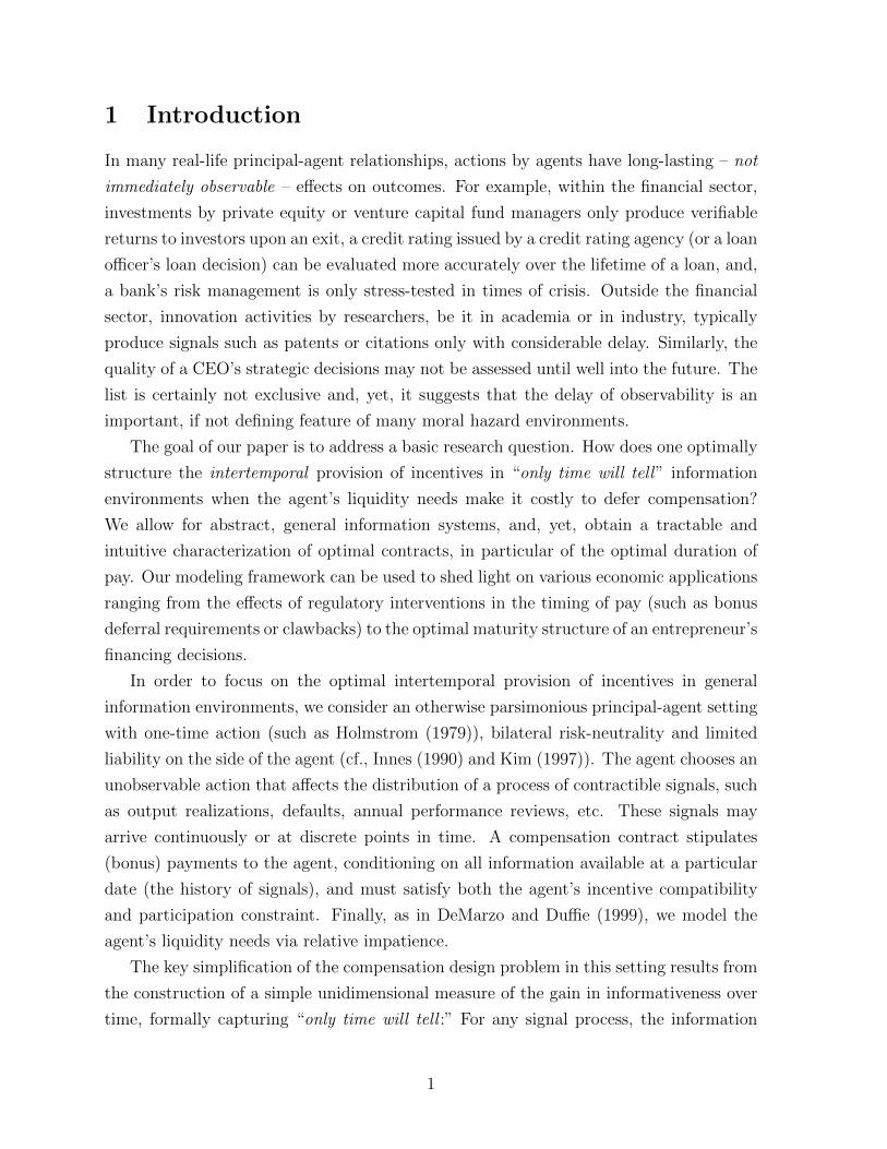
left panel of Figure 1 for an example). This benefit of deferral encoded in I (t), however,
comes at a cost due to the agent’s relative impatience.
0 t$ 7T
Time t
1
e"rt$
e"r 7T Impatience Cost e"rt
Informativeness I(t)
0 I(t$) I( 7T )
Contract Informativeness IC
1
e"rt$
e"r 7T C(IC)6C(IC)
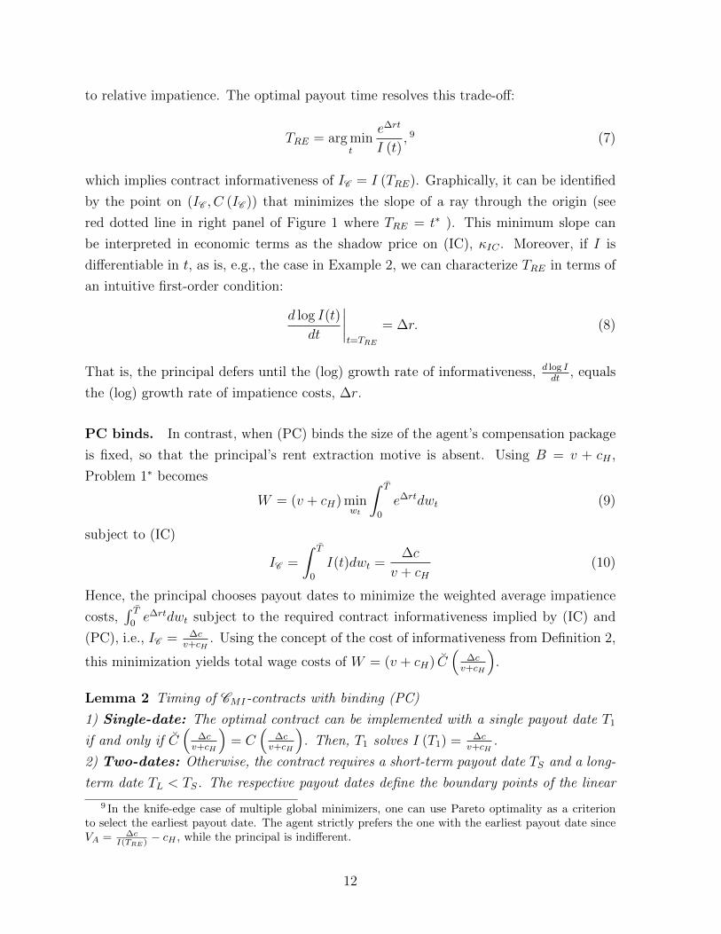
Figure 1. Impatience costs versus informativeness: The left panel plots both impatiencecosts, e∆rt, and maximal informativeness, I (t), as a function of time t for an example economy thatfeatures a significant increase in informativeness at date t∗. The right panel plots the function Cand its lower convex envelope C against contract informativeness IC . The solid circles in the leftand right panel correspond to the boundary points that define the cost of informativeness C (IC ).
10
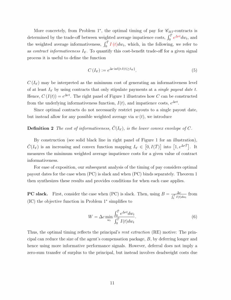
More concretely, from Problem 1∗, the optimal timing of pay for CMI-contracts is
determined by the trade-off between weighted average impatience costs,∫ T
0e∆rtdwt, and
the weighted average informativeness,∫ T
0I (t)dwt, which, in the following, we refer to
as contract informativeness IC . To quantify this cost-benefit trade-off for a given signal
process it is useful to define the function
C (IC ) := e∆r inf{t:I(t)≥IC }. (5)
C (IC ) may be interpreted as the minimum cost of generating an informativeness level
of at least IC by using contracts that only stipulate payments at a single payout date t.
Hence, C (I(t)) = e∆rt. The right panel of Figure 1 illustrates how C can be constructed
from the underlying informativeness function, I(t), and impatience costs, e∆rt.
Since optimal contracts do not necessarily restrict payouts to a single payout date,
but instead allow for any possible weighted average via w (t), we introduce
Definition 2 The cost of informativeness, C(IC ), is the lower convex envelope of C.
By construction (see solid black line in right panel of Figure 1 for an illustration),
C(IC ) is an increasing and convex function mapping IC ∈[0, I(T )
]into
[1, e∆rT
]. It
measures the minimum weighted average impatience costs for a given value of contract
informativeness.
For ease of exposition, our subsequent analysis of the timing of pay considers optimal
payout dates for the case when (PC) is slack and when (PC) binds separately. Theorem 1
then synthesizes these results and provides conditions for when each case applies.
PC slack. First, consider the case when (PC) is slack. Then, using B = ∆c∫ T0 I(t)dwt
from
(IC) the objective function in Problem 1∗ simplifies to
W = ∆cminwt
∫ T0e∆rtdwt∫ T
0I(t)dwt
. (6)
Thus, the optimal timing reflects the principal’s rent extraction (RE) motive: The prin-
cipal can reduce the size of the agent’s compensation package, B, by deferring longer and
hence using more informative performance signals. However, deferral does not imply a
zero-sum transfer of surplus to the principal, but instead involves deadweight costs due
11
to relative impatience. The optimal payout time resolves this trade-off:
TRE = arg mint
e∆rt
I (t), 9 (7)
which implies contract informativeness of IC = I (TRE). Graphically, it can be identified
by the point on (IC , C (IC )) that minimizes the slope of a ray through the origin (see
red dotted line in right panel of Figure 1 where TRE = t∗ ). This minimum slope can
be interpreted in economic terms as the shadow price on (IC), κIC . Moreover, if I is
differentiable in t, as is, e.g., the case in Example 2, we can characterize TRE in terms of
an intuitive first-order condition:
d log I(t)
dt
∣∣∣∣t=TRE
= ∆r. (8)
That is, the principal defers until the (log) growth rate of informativeness, d log Idt
, equals
the (log) growth rate of impatience costs, ∆r.
PC binds. In contrast, when (PC) binds the size of the agent’s compensation package
is fixed, so that the principal’s rent extraction motive is absent. Using B = v + cH ,
Problem 1∗ becomes
W = (v + cH) minwt
∫ T
0
e∆rtdwt (9)
subject to (IC)
IC =
∫ T
0
I(t)dwt =∆c
v + cH(10)
Hence, the principal chooses payout dates to minimize the weighted average impatience
costs,∫ T
0e∆rtdwt subject to the required contract informativeness implied by (IC) and
(PC), i.e., IC = ∆cv+cH
. Using the concept of the cost of informativeness from Definition 2,
this minimization yields total wage costs of W = (v + cH) C(
∆cv+cH
).
Lemma 2 Timing of CMI-contracts with binding (PC)
1) Single-date: The optimal contract can be implemented with a single payout date T1
if and only if C(
∆cv+cH
)= C
(∆cv+cH
). Then, T1 solves I (T1) = ∆c
v+cH.
2) Two-dates: Otherwise, the contract requires a short-term payout date TS and a long-
term date TL < TS. The respective payout dates define the boundary points of the linear
9 In the knife-edge case of multiple global minimizers, one can use Pareto optimality as a criterionto select the earliest payout date. The agent strictly prefers the one with the earliest payout date sinceVA = ∆c
I(TRE) − cH , while the principal is indifferent.
12
segment of C that contains IC = ∆cv+cH
. The fraction of B derived from payouts at date
TS is given by wS =I(TL)− ∆c
v+cH
I(TL)−I(TS).
0 T1 TRE t
1
e"rt
I(t)
0 "c
v + cH
I(TRE) IC
1
e"rT1
Single payout date
C(IC)6C(IC)
0 TS T1 TL t
1
e"rt
I(t)
0 I(TS) "c
v + cH
I(TL) IC
1
e"rT1
Two payout dates
C(IC)6C(IC)
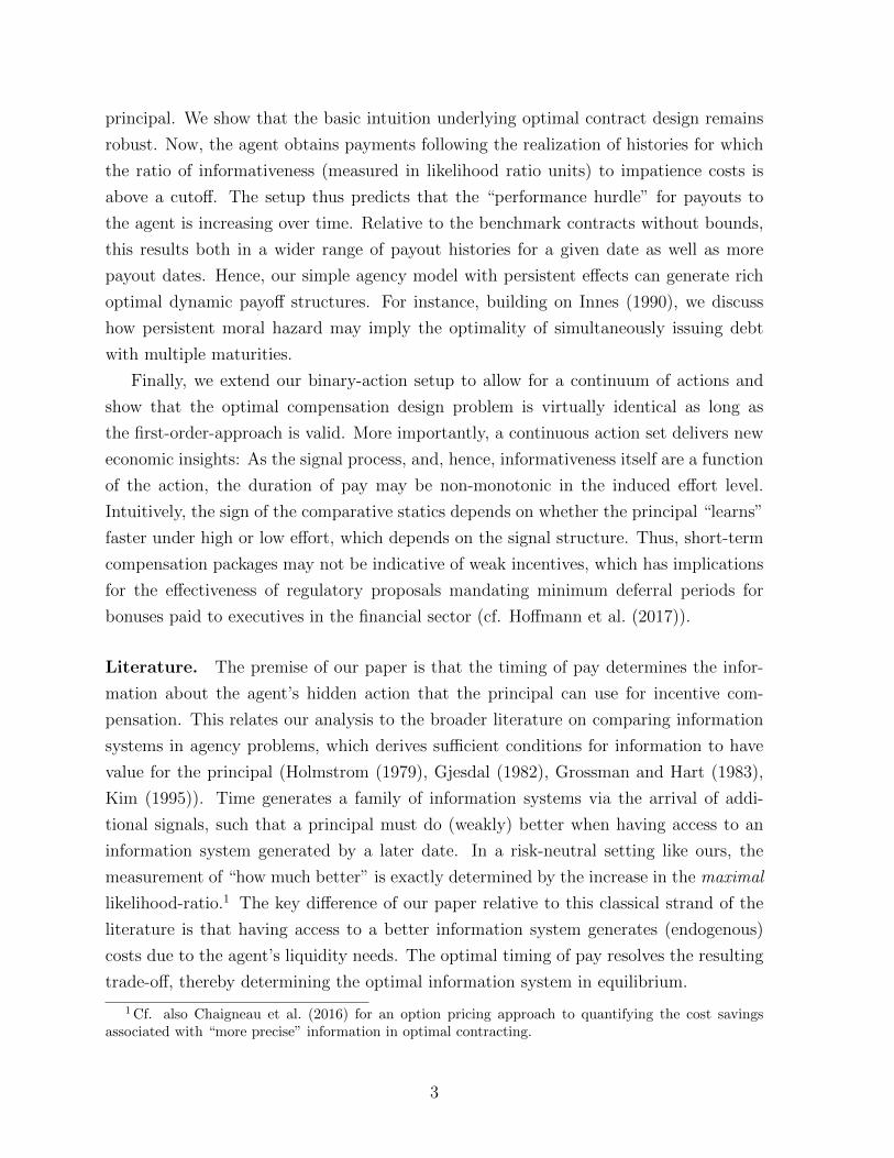
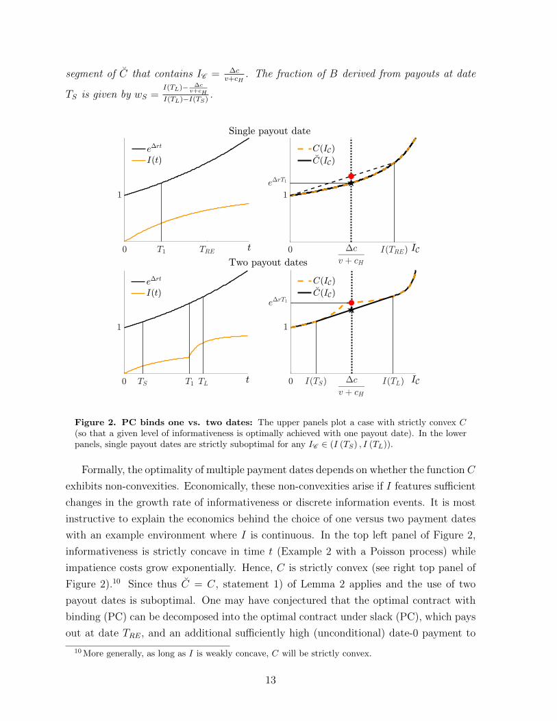
Figure 2. PC binds one vs. two dates: The upper panels plot a case with strictly convex C(so that a given level of informativeness is optimally achieved with one payout date). In the lowerpanels, single payout dates are strictly suboptimal for any IC ∈ (I (TS) , I (TL)).
Formally, the optimality of multiple payment dates depends on whether the function C
exhibits non-convexities. Economically, these non-convexities arise if I features sufficient
changes in the growth rate of informativeness or discrete information events. It is most
instructive to explain the economics behind the choice of one versus two payment dates
with an example environment where I is continuous. In the top left panel of Figure 2,
informativeness is strictly concave in time t (Example 2 with a Poisson process) while
impatience costs grow exponentially. Hence, C is strictly convex (see right top panel of
Figure 2).10 Since thus C = C, statement 1) of Lemma 2 applies and the use of two
payout dates is suboptimal. One may have conjectured that the optimal contract with
binding (PC) can be decomposed into the optimal contract under slack (PC), which pays
out at date TRE, and an additional sufficiently high (unconditional) date-0 payment to
10 More generally, as long as I is weakly concave, C will be strictly convex.
13
satisfy (PC). This conjecture is typically wrong. The candidate contract (indicated by
the red circle in right top panel of Figure 2) turns out to produce strictly higher wage
costs to the principal than the optimal contract with a single payout date at T1 (indicated
by the black star).
In contrast, in the bottom left panel of Figure 2, the underlying informativeness
process features two phases of high growth. As a result, the impatience costs associated
with single-date contracts exhibit non-convexities (see bottom right panel of Figure 2).
To tap “late” increases in informativeness, the optimal contract now makes a payment
at a long-term date TL to target (IC) and an additional short-term payment at date TS
to satisfy (PC) at lower impatience costs. The optimal choice of TS and TL generates a
strict improvement over the single-date contract that pays out exclusively at date T1 (see
red circle in top right panel).
2.2.3 Optimal contracts and comparative statics
Synthesizing the cases with (PC) binding and (PC) slack, we can now fully characterize
optimal contracts. Together with the conditions for the optimality of CMI-contracts
derived in Lemma 1 we thereby obtain a characterization of optimal contracts based on
the solution to Problem 1∗. For completeness, the characterization also includes the less
interesting case when (IC) is slack (κIC = 0).
Theorem 1 The optimal contract is characterized as follows:
1. If v ≤ v = ∆cI(TRE)
− cH , (PC) is slack. The optimal payout date is T ∗ = TRE as
defined in (7) and the size of the compensation package is B∗ = ∆cI(TRE)
.
2. If v > v, (PC) binds, so that B∗ = v + cH and IC = ∆cv+cH
. If I (0) ≤ ∆cv+cH
, (IC)
binds and the optimal contract requires at max two payout dates T ∗ as characterized
in Lemma 2. If I (0) > ∆cv+cH
, (IC) is slack and all payments are made at date 0.
Theorem 1 summarizes the intuitive characterization of the timing of optimal con-
tracts in general information environments. From this characterization we also obtain
the associated wage cost to the principal:
W =
∆c
I(TRE)e∆rTRE
(v + cH) C(
∆cv+cH
) v ≤ v
v > v. (11)
Depending on the particular application at hand (cf., Section 4), W can then be
substituted into the principal’s objective function to determine whether implementing
aH is indeed optimal, the second step in the structure of Grossman and Hart (1983).
14

Using the characterization of the optimal timing of pay in Theorem 1, it is now also
possible to analyze its comparative statics
Corollary 1 The duration of the compensation package∫tdw∗t is decreasing in v and
increasing in ∆c.
The comparative statics in v and ∆c follow from the fact that the size of the com-
pensation package, B, and more informative performance signals, IC , are substitutes for
providing incentives to the agent, i.e., BIC = ∆c. When an increase in the agent’s outside
option v exogenously raises the size of pay, this substitutability implies that the principal
optimally shortens the duration of the compensation package, such as to reduce contract
informativeness (strictly so if (IC) and (PC) bind). In contrast, if the agency problem
gets more severe, i.e., ∆c increases, then the principal relies on both more informative
performance signals and a larger compensation package. In Section 3.2, we extend our
setup to a continuous action set, which allows us to characterize the non-trivial compar-
ative statics of payout times in the action choice a.
3 Extensions
3.1 Payment bounds
So far, the focus of our paper was to provide a tractable characterization of the optimal
timing of pay (see Theorem 1). The associated maximal-incentives contracts have stark
implications in that they may prescribe high rewards for low-probability events. However,
many real-life contracts do not exclusively stipulate payments for the most informative
signal histories and also have a wider selection of payment dates. One way to capture
these additional realistic contract features without losing tractability is to incorporate
(upper) bounds on payments (see also Jewitt et al. (2008)). Bounds on payments may
be economically motivated by a physical resource constraint, such as the principal’s
limited liability, regulatory constraints, such as bonus caps, or arise endogenously via the
agent’s risk-aversion (see Plantin and Tirole (2015)). Apart from this applied motivation,
the introduction of bounds has the technical benefit that they allow us to eliminate
Assumption 1 from now on, and, hence, extend our analysis to information settings
where a solution to the original Problem 1 does not exist.
For ease of exposition, we suppose that there be a constraint k > 0 on the payment
rate that can be paid out to the agent, i.e., dbt ≤ kdt.11 Following Plantin and Tirole
11 We note that a more general specification of payment bounds, say dbt ≤ dk (ht), would yield
15
(2015), one way to rationalize this particular form of a bound is to appeal to a simple form
of risk aversion on the side of the agent: Her marginal utility from (flow) consumption
at any given point of time drops from one to zero when it exceeds k.12 For brevity’s sake
we restrict consideration to the case where v = 0 and I (0) < ∆ccH, so that (PC) is slack
and (IC) binds. Moreover, we suppose that aH is implementable even in the presence of
bounds.
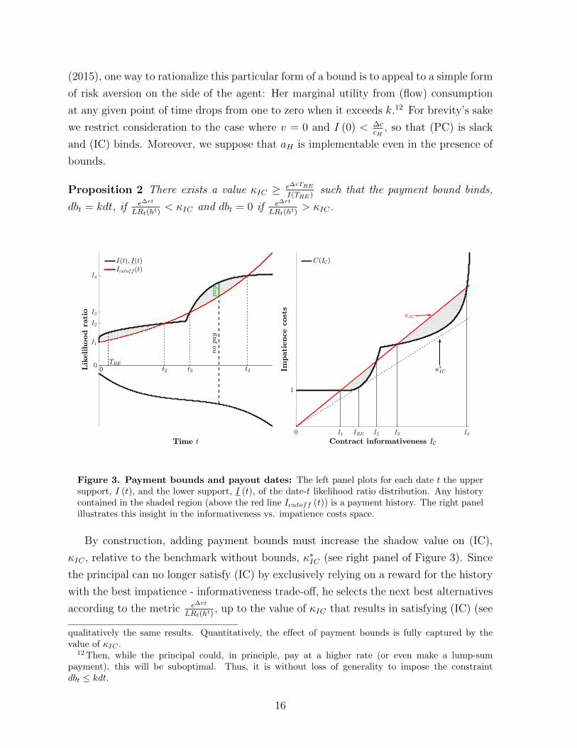
Proposition 2 There exists a value κIC ≥ e∆rTRE
I(TRE)such that the payment bound binds,
dbt = kdt, if e∆rt
LRt(ht)< κIC and dbt = 0 if e∆rt
LRt(ht)> κIC.
Time t
0
I1
I2
I3
I4
Lik
elihood
rati
o
no
pay
pay
I(t); I(t)Icutoff (t)
0 I1 IRE I2 I3 I4
Contract informativeness IC
1
Impati
ence
cost
s
C(IC)
TRE
0 t2 t4t3 5$IC
5IC
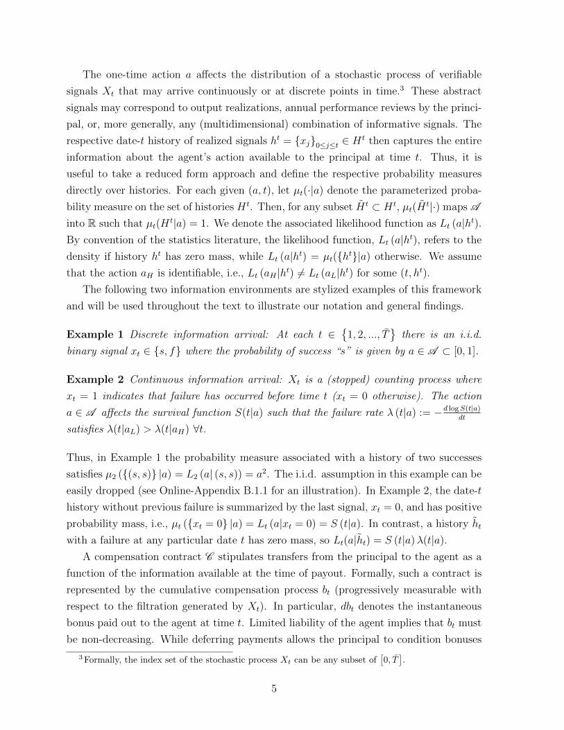
Figure 3. Payment bounds and payout dates: The left panel plots for each date t the uppersupport, I (t), and the lower support, I (t), of the date-t likelihood ratio distribution. Any historycontained in the shaded region (above the red line Icutoff (t)) is a payment history. The right panelillustrates this insight in the informativeness vs. impatience costs space.
By construction, adding payment bounds must increase the shadow value on (IC),
κIC , relative to the benchmark without bounds, κ∗IC (see right panel of Figure 3). Since
the principal can no longer satisfy (IC) by exclusively relying on a reward for the history
with the best impatience - informativeness trade-off, he selects the next best alternatives
according to the metric e∆rt
LRt(ht), up to the value of κIC that results in satisfying (IC) (see
qualitatively the same results. Quantitatively, the effect of payment bounds is fully captured by thevalue of κIC .
12 Then, while the principal could, in principle, pay at a higher rate (or even make a lump-sumpayment), this will be suboptimal. Thus, it is without loss of generality to impose the constraintdbt ≤ kdt.
16
histories contained in the shaded region of the right panel of Figure 3). Then, given
κIC , the left panel of Figure 3 traces out the cutoff for the date-t likelihood ratio that
results in payments to the agent, Icutoff (t) := e∆rt
κIC.13 Thus, the performance “hurdle”
for obtaining payments increases over time at a rate of ∆r. For the example signal
process, this implies two disconnected time intervals of payment dates [t1, t2] and [t3, t4].
In Online-Appendix B.1.2 we show the effects of payment bounds within our Example 2.
3.2 Continuous actions
We finally extend our analysis to a continuous action set, a ∈ A = [0, a], which allows
for additional comparative statics analysis. The associated cost function c (a) satisfies
the usual conditions, i.e., it is strictly increasing and strictly convex with c(0) = c′(0) = 0
as well as c′(a) = ∞. To mirror the structure of our analysis so far, we will focus on
optimal compensation design, i.e., characterize cost-minimizing contracts to implement a
given action a (the first problem in Grossman and Hart (1983)) and relegate the optimal
action choice by the principal to Online-Appendix B.2.
Our key object is now the log likelihood ratio (score), d logLt
da, the analog of LRt(h
t)
for continuous actions. We impose standard Cramer-Rao regularity conditions used in
statistical inference (cf. e.g., Casella and Berger (2002)): In particular, the score, d logLt
da,
exists and is bounded for any (t, ht). We then adjust our preceding notation as follows:
htMI (a) := arg maxht∈Ht
d logLt (a|ht)da
(12)
I (t|a) := maxht∈Ht
d logLt (a|ht)da
=d logLt (a|htMI)
da.14 (13)
As the scored logLt(a|ht)
dais a martingale, I (t|a) is an increasing function of time (cf.,
Proposition 1).15
As is common in static moral hazard problems with continuous actions (see e.g.,
Holmstrom (1979) and Shavell (1979)) we assume that the first-order approach is valid.
Hence, for each a, we replace (IC) by the following first-order condition
∂
∂aE
[∫ T
0
e−rAtdbt
∣∣∣∣∣ a]
= c′ (a) . (IC-FOC)
13 Clearly, histories with a negative likelihood ratio will never be selected (cf. the weakly decreasinglower support of the likelihood ratio distribution depicted in the left panel of Figure 3, I(t) < Icutoff (t)).
14The function I (t|a) is similar to the well known Fisher information function in statistics, which fora given t, is defined as the variance of the score across histories.
15 The score is no longer bounded above by one, but this is irrelevant for the further analysis.
17
It is immediate that our preceding characterization now readily extends to the continuous
action case as long as (IC) is relevant for compensation costs. For completeness, we
restate Theorem 1 in Online-Appendix B.2. It is now also possible to provide a sufficient
condition for the validity of the first-order approach.
Lemma 3 If Lt(a|hTMI (a)
)is strictly concave in a for the optimal payout dates T ∗(a),
then the first-order approach is valid for action a.16
We conclude by conducting a comparative statics analysis of the duration of pay,∫tdw∗t , in the incentivized action a. Does higher effort optimally require further defer-
ral? The associated analysis makes it transparent how the learning process, and hence
informativeness itself, I(t|a), are now a function of the implemented action. One may
thus already conjecture that the comparative statics are subtle and ought to depend on
the characteristics of the signal process.
For brevity’s sake we focus on the case when (PC) is slack.17 The optimal payment
date associated with action a then satisfies: T ∗(a) = TRE (a) = arg minte∆rt
I(t|a). The
comparative statics thus depend on whether the principal learns faster under high or
low effort. To provide further intuition, we assume that I is differentiable, so that the
first-order condition in (8) applies. Then, the sign of the comparative statics of contract
duration TRE (a) in a depends on whether the (log) growth rate of informativeness, d log Idt
,
increases or decreases in a, i.e.,
sgn
(dTRE (a)
da
)= sgn
(d
da
d log I(t|a)
dt
∣∣∣∣t=TRE(a)
). (14)
To illustrate that all comparative statics are generically possible even within our
Example 2, we make use of three commonly used parametric survival time distributions.18
Example 2.1 Mixed distribution: S(t|a) = aSL(t) + (1− a)SH(t) with a ∈ [0, 1] and
where SL(t) dominates SH(t) in the hazard rate order, i.e., λL(t) < λH(t).
Example 2.2 Exponential distribution: S(t|a) = e−ta , with a > 0.
Example 2.3 Log-normal distribution: S(t|a) = 12− 1
2erf[
log t−a√2σ
], with a ≥ 0, σ > 0.
16 The condition is reminiscent of the convexity of the distribution function condition (CDFC) in staticmodels (cf. e.g., Rogerson (1985)).
17 The main takeaways equally apply to the case where (PC) binds.18 We note that for Example 2.2 and 2.3 the validity of the first-order approach must be ensured via
appropriate parametrization.
18
First, we consider the benchmark case of an exponential distribution (Example 2.2).
With a continuous action set, any i.i.d. process yields an informativeness function that
is linear in time (here: I(t|a) = ta2 ). As a result, the log-growth rate is independent of
the action, i.e., 1t, implying a payout date of TRE (a) = 1
∆rfor all actions a. In this case
(and for all other i.i.d. processes), the timing of the bonus alone would not provide any
information about the induced action. In contrast, in Example 2.1 information grows
faster for lower effort so that a shorter duration is indicative of higher, rather than lower
incentives. The opposite comparative static holds for Example 2.3. Knowledge of the
information process (and how it is influenced by the action) is thus crucial for making
predictions about the optimal timing of pay.
Our results suggest that the empirical analysis of compensation contracts ought to
relate the timing dimension of pay also to variation in the nature of information arrival
across industries (see e.g., Gopalan et al. (2014)). For example, it may be hypothesized
that firms in R&D intensive industries (with year-long lags and few products) ought to
design longer-duration contracts for their CEOs.
4 Applications
We conclude with three potential applications of our basic framework and its extensions.
First, our framework can be used to understand the effects of regulatory interventions in
the timing of pay, such as minimum deferral periods or clawback clauses. For example,
in the United Kingdom, the regulator has recently started to impose a minimum deferral
period of 3 years and a clawback period of 7 years for bonuses to executives in the
financial sector. It is thus a timely policy question to analyze the effect of such regulations
on the action that the principal, the board of a bank, induces in equilibrium. In the
absence of any regulation, the board may choose to implement actions that primarily
exploit tax payer guarantees. Does deferral regulation nudge the principal to implement
better actions? While minimum deferral regulation (trivially) increases wage costs for all
actions, we show in our companion paper Hoffmann et al. (2017), that it can work akin to
a Pigouvian tax if it taxes wage costs of actions that are “bad” from a society’s perspective
more than wage costs of “good” actions. The effectiveness of deferral clauses is thus
intimately linked to the comparative statics analysis of payout times: If the principal’s
unconstrained compensation design features longer payout dates for those actions that
are better from a society’s perspective, then deferral regulation can be effective by making
better actions relatively cheaper.
Second, our framework lends itself to develop an incentive-based theory of debt ma-
19
turity. As shown by Innes (1990), if signals correspond to output realizations satisfying
MLRP and one imposes a monotonicity constraint on the principal’s payoff, the optimal
contract for outside financing is a debt contract (inside equity). Within our dynamic
framework, it is now possible to solve for the optimal dynamic payoff structure. Building
on our analysis of payment bounds in Section 3.1, a simple moral hazard problem with
persistent effects can give rise to a complex maturity structure of insiders’ and outsiders’
claims (similar to Figure 3), resulting from the trade-off between the entrepreneur’s liq-
uidity needs and the increased informativeness associated with new performance signals
available to investors. Different from our previous analysis, payment bounds at a par-
ticular point in time t should then, however, depend both on the history ht and on the
endogenously chosen payouts (dividends, sale of equity stakes) at earlier points in time.
Finally, it is possible to give the principal a more active role by allowing him to in-
vest directly in information (accounting) systems. For example, one can imagine many
settings where the principal can also acquire costly signals about the agent’s action, say
via costly monitoring and auditing and not just wait for information (see Plantin and
Tirole (2015) for a similar mechanism). It is now possible to analyze the optimal mix
of information sources. The difference between these two types of investments in infor-
mation is that the costs associated with deferral are endogenous in that the impatience
costs interact with the size of the deferred bonus package, whereas investments in IT or
accounting systems are lump sum.
Appendix A Proofs
Proof of Lemma 1. We will start with some useful definitions: Let B denote theagent’s expected time-0 valuation of the compensation package, i.e.,
B := E
[∫ T
0
e−rAtdbt
∣∣∣∣∣ aH],
and denote by wt the fraction of the compensation package that the agent derives fromexpected payouts up to time t ≤ T , i.e.,
wt := E[∫ t
0
e−rAsdbs
∣∣∣∣ aH] /B,so that wT =
∫ T0dwt = 1. Further, denote, for each given t, the maximal likelihood ratio
by I(t) := maxht∈Ht LRt(ht) which exists by Assumption 1. Using the definition of B,
20
the incentive constraint (IC) can be written as:
B
1−E[∫ T
0e−rAtdbt
∣∣∣ aL]E[∫ T
0e−rAtdbt
∣∣∣ aH] ≥ ∆c.
Given the definition of LRt(ht) = 1− Lt(aL|ht)
Lt(aH |ht), we may write this incentive constraint as:
B
(∫ T
0
[∫Ht
LRt(ht|aH)dγt(h
t)
]dwt
)≥ ∆c, (15)
for some weighing function γt(ht) satisfying dγt(h
t) ≥ 0 and∫Ht dγt(h
t) = 1. The follow-ing Lemma shows when (IC) binds, i.e., is relevant for compensation costs.
Lemma A.1 The shadow value on (IC), κIC, is zero if and only if I(0) ≥ ∆cv+cH
.
Proof of Lemma A.1 From (PC) and (LL) together with differential discounting wehave that W ≥ v+cH . Hence, we need to show that W = v+cH if and only if I(0) ≥ ∆c
v+cH.
To show sufficiency, consider the CMI-contract delivering total expected payB = (v + cH)with a single payment at t = 0. This contract trivially satisfies (PC) and (LL), as wellas, from I(0) ≥ ∆c
v+cHalso (IC), and implies expected wage costs of v + cH . To show the
necessary part, observe that any contract with W = v + cH cannot feature any delaydue to differential discounting, i.e., must satisfy w0 = 1. Note further, that the contractthat provides strongest incentives with date-0 payments only is, from (15), the one thatmakes the entire expected pay B contingent on h0
MI . However, whenever I(0) < ∆cv+cH
,such a contract requires B > v + cH in order to satisfy (IC), implying W > v + cH . �
Take now the case where κIC > 0, implying W = B∫ T
0e∆rtdwt > v + cH . The
proof then is by contradiction. So assume that under the optimal contract there existssome t for which
∫Ht\htMI
dγt(ht) 6= 0. Then, there exists another feasible contract with∫
Ht\htMIdγt(h
t) = 0 for all t and strictly lower compensation costs. To see this, observe
that this new contract maximizes, for given wt and B, the left-hand side in (15). So,assume, first, that (PC) is slack. Then, holding wt constant, the new contract allowsfor a strictly lower B, thus reducing W . Second, assume that (PC) binds, which, fromκIC > 0 implies that w0 < 1. Then, holding B constant, the new contract allows toreduce some wt, t > 0, and increase w0 resulting in lower W . Finally, that there existsan optimal contract from the class of CMI contracts when κIC = 0 follows directly fromthe construction in the proof of Lemma A.1. Q.E.D.
Proof of Proposition 1. The result follows from the well-known fact that LRt(ht)
as defined in (2) is a martingale (see e.g., Casella and Berger (2002)) and for each t weconsider the maximal realization. Q.E.D.
Proof of Lemma 2. As has been shown in the main text, the optimal CMI-contractwith binding participation constraint requires contract informativeness of IC = ∆c
v+cH
21
with associated cost of informativeness of C( ∆cv+cH
). As C(IC ) is the lower convex enve-lope of C(IC ), the cost of informativeness associated with contracts stipulating a singlepayout date, it is immediate that at most 2 payout dates are sufficient for achievingC( ∆c
v+cH). These are generally characterized by IS = I(TS) and IL = I(TL), where IS =
sup{IC ≤ ∆c
v+cH: C(IC ) = C(IC )
}and IL = inf
{IC ≥ ∆c
v+cH: C(IC ) = C(IC )
}, which we
refer to as the boundary points of C(IC ) around IC = ∆cv+cH
. If C( ∆cv+cH
) = C( ∆cv+cH
) wehave IS = IL and, hence, B is paid out at a single date TS = TL =: T1. Else, thereare two payments, TS < TL and the fraction of B paid out at TS is obtained from (10).Q.E.D.
Proof of Theorem 1. It follows from Lemma 1 that, given Assumption 1, Problem 1has a solution within the class of CMI-contracts, i.e., the solution to Problem 1∗ solvesProblem 1. Consider now, first, the relaxed problem ignoring (PC). Then, as shown inthe main text, the optimal payout time is given by TRE as characterized in (7) whichimplies from (IC) that B = ∆c/I (TRE). Then (PC) is indeed satisfied, such that thesolution to the relaxed problem solves the full problem, if and only if B ≥ v + cH whichis equivalent to v ≤ v := ∆c/I (TRE)− cH . Else, it is easy to show that (PC) must bindunder the optimal contract, i.e., B = v+ cH . The optimal timing of pay then depends onwhether (IC) is relevant for compensation costs, which from Lemma A.1 is the case if andonly if I(0) < ∆c
v+cH. Hence, if I(0) < ∆c
v+cH, the optimal payout times are as characterized
in Lemma 2, while for I(0) ≥ ∆cv+cH
all payouts are made at date 0. Q.E.D.
Proof of Corollary 1. From Theorem 1, these comparative statics hold trivially ifI (TRE) < ∆c
v+cHso that PC is slack. In this regime 1, the duration TRE does not depend
on v and ∆c. When I (TRE) ≥ ∆cv+cH
> I(0), PC and IC bind (regime 2), the result
follows directly from IC = ∆cv+cH
, which is decreasing in v and increasing in ∆c, together
with Lemma 2. Finally, when I (TRE) ≥ I(0) ≥ ∆cv+cH
, IC is slack (regime 3) and theduration is equal to zero independently of v and ∆c. Now note that, as v increases or∆c decreases, we either stay within each regime or move from regime 1 to regime 2 toregime 3 and the result follows. Q.E.D.
Proof of Lemma 3. The assumption in the Lemma is sufficient to ensure that, given acontract as characterized in Theorem B.1, the agent’s problem maxa {VA(a)} is strictlyconcave. Hence, the first-order condition in (IC-FOC) is both necessary and sufficientfor incentive compatibility. Q.E.D.
Proof of Proposition 2. With pay caps, the incentive constraint can still be writtenas (15) but now with the additional restriction that Bdγt(h
t)dwt ≤ kdt. Hence, when(IC) binds and (PC) is slack we can write in analogy to (6)
W = ∆cminwt
∫ T0
∫Ht e
∆rtdγt(ht)dwt∫ T
0
∫Ht LRt(ht)dγt(ht)dwt
,
and the result immediately follows. Q.E.D.
22
References
Casella, G., and R. L. Berger, 2002, Statistical inference, volume 2 (Duxbury PacificGrove, CA).
Chaigneau, P., A. Edmans, and D. Gottlieb, 2016, The value of informativeness forcontracting, Working Paper 20542, National Bureau of Economic Research.
DeMarzo, P., and D. Duffie, 1999, A liquidity-based model of security design, Economet-rica 67, 65–99.
DeMarzo, P. M., and Y. Sannikov, 2006, Optimal security design and dynamic capitalstructure in a continuous-time agency model, Journal of Finance 61, 2681–2724.
Fudenberg, D., and J. Tirole, 1990, Moral hazard and renegotiation in agency contracts,Econometrica 58, 1279–1319.
Gjesdal, F., 1982, Information and incentives: The agency information problem, TheReview of Economic Studies 49, 373–390.
Gopalan, R., T. Milbourn, F. Song, and A. V. Thakor, 2014, Duration of executivecompensation, The Journal of Finance 69, 2777–2817.
Grossman, S. J., and O. D. Hart, 1983, An analysis of the principal-agent problem,Econometrica 51, 7–45.
Hartman-Glaser, B., T. Piskorski, and A. Tchistyi, 2012, Optimal securitization withmoral hazard, Journal of Financial Economics 104, 186 – 202.
Hermalin, B. E., and M. L. Katz, 1991, Moral hazard and verifiability: The effects ofrenegotiation in agency, Econometrica 59, 1735–1753.
Hoffmann, F., R. Inderst, and M. M. Opp, 2017, Regulating deferred incentive pay,Technical report, University of Bonn, University of Frankfurt, University of California,Berkeley.
Holmstrom, B., 1979, Moral hazard and observability, Bell Journal of Economics 10,74–91.
Hopenhayn, H., and A. Jarque, 2010, Unobservable persistent productivity and long termcontracts, Review of Economic Dynamics 13, 333 – 349.
Innes, R. D., 1990, Limited liability and incentive contracting with ex-ante action choices,Journal of Economic Theory 52, 45–67.
Jarque, A., 2010, Repeated moral hazard with effort persistence, Journal of EconomicTheory 145, 2412–2423.
Jewitt, I., O. Kadan, and J. M. Swinkels, 2008, Moral hazard with bounded payments,Journal of Economic Theory 143, 59 – 82.
23
Kim, S. K., 1995, Efficiency of an information system in an agency model, Econometrica63, 89–102.
Kim, S. K., 1997, Limited liability and bonus contracts, Journal of Economics and Man-agement Strategy 6, 899–913.
Malamud, S., H. Rui, and A. Whinston, 2013, Optimal incentives and securitization ofdefaultable assets, Journal of Financial Economics 107, 111 – 135.
Manso, G., 2011, Motivating innovation, The Journal of Finance 66, 1823–1860.
Opp, M. M., and J. Y. Zhu, 2015, Impatience versus incentives, Econometrica 83, 1601–1617.
Plantin, G., and J. Tirole, 2015, Marking to market versus taking to market, Technicalreport, Toulouse School of Economics.
Ray, D., 2002, The time structure of self-enforcing agreements, Econometrica 70, 547–582.
Rogerson, W. P., 1985, The first-order approach to principal-agent problems, Economet-rica 53, 1357–67.
Sannikov, Y., 2014, Moral hazard and long-run incentives, Unpublished working paper,Princeton University.
Shavell, S., 1979, Risk sharing and incentives in the principal and agent relationship, TheBell Journal of Economics 10, 55–73.
Tirole, J., 2005, Theory of Corporate Finance (Princeton University Press, Princeton).
Zhu, J., 2017, Myopic agency, Review of Economic Studies forthcoming.
24
Appendix B Online-Appendix
B.1 Further results for binary action set
B.1.1 Non-i.i.d. example
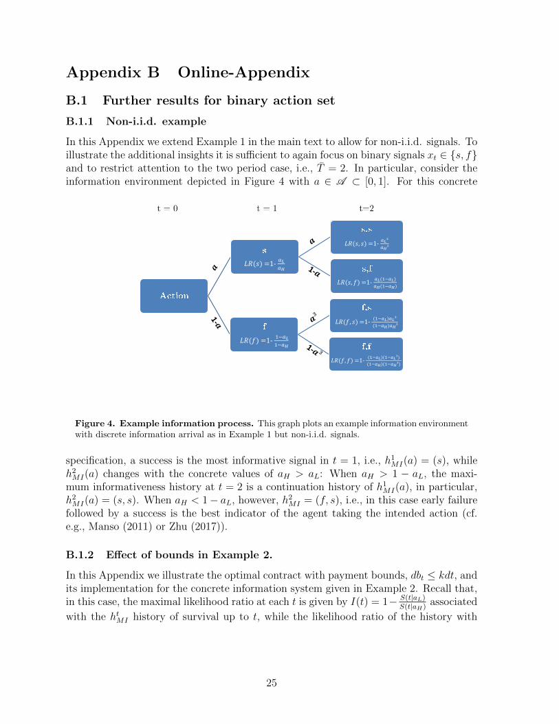
In this Appendix we extend Example 1 in the main text to allow for non-i.i.d. signals. Toillustrate the additional insights it is sufficient to again focus on binary signals xt ∈ {s, f}and to restrict attention to the two period case, i.e., T = 2. In particular, consider theinformation environment depicted in Figure 4 with a ∈ A ⊂ [0, 1]. For this concrete
𝐿𝑅(𝑠)=1-𝑎𝐿
𝑎𝐻
𝐿𝑅(𝑠, 𝑠) =1-𝑎𝐿²
𝑎𝐻²
𝐿𝑅(𝑠, 𝑓)=1-𝑎𝐿(1−𝑎𝐿)
𝑎𝐻(1−𝑎𝐻)
𝐿𝑅(𝑓) =1-1−𝑎𝐿
1−𝑎𝐻
𝐿𝑅(𝑓, 𝑠)=1-(1−𝑎𝐿)𝑎𝐿³
(1−𝑎𝐻)𝑎𝐻³
𝐿𝑅(𝑓, 𝑓)=1-(1−𝑎𝐿)(1−𝑎𝐿³)
(1−𝑎𝐻)(1−𝑎𝐻³)
Figure 4. Example information process. This graph plots an example information environmentwith discrete information arrival as in Example 1 but non-i.i.d. signals.
specification, a success is the most informative signal in t = 1, i.e., h1MI(a) = (s), while
h2MI(a) changes with the concrete values of aH > aL: When aH > 1 − aL, the maxi-
mum informativeness history at t = 2 is a continuation history of h1MI(a), in particular,
h2MI(a) = (s, s). When aH < 1− aL, however, h2
MI = (f, s), i.e., in this case early failurefollowed by a success is the best indicator of the agent taking the intended action (cf.e.g., Manso (2011) or Zhu (2017)).
B.1.2 Effect of bounds in Example 2.
In this Appendix we illustrate the optimal contract with payment bounds, dbt ≤ kdt, andits implementation for the concrete information system given in Example 2. Recall that,in this case, the maximal likelihood ratio at each t is given by I(t) = 1− S(t|aL)
S(t|aH)associated
with the htMI history of survival up to t, while the likelihood ratio of the history with
25
failure at time t which we denote by htf is given by
LRt(htf ) = 1−
Lt(aL|htf
)Lt(aH |htf
) = 1− S (t|aL)
S (t|aH)
λ(t|aL)
λ(t|aH)
= I (t)− [1− I (t)]
[λ(t|aL)
λ(t|aH)− 1
].
Clearly, LRt(htf ) < I (t) for all finite t, but for t sufficiently large it holds that LRt(h
tf ) > 0
such that a payment following htf provides incentives.19 To complete the description ofthe likelihood ratio process, note that conditional on failure at some t = t′, the likelihoodratio stays constant at LRt′(h
t′
f ) for all t ≥ t′ as no further information is revealed. It isthen easy to see from the characterization in Proposition 2 that, for a sufficiently tightpayment bound (i.e., a sufficiently high κIC), rewards following failure become optimal.In particular, as the likelihood ratio stays constant following failure, it will be optimal topay the agent in a time interval following failure at t as long as e∆rt/LRt(h
tf ) < κIC .20
Within our interpretation of payment bounds as a reduced form modeling of agent riskaversion, these payments can simply be implemented by making a lump-sum “goldenparachute” payment at the time of failure, which the agent then consumes over therespective interval.
B.2 Continuous action set
B.2.1 Optimal compensation design
In this Appendix, we formally characterize the optimal contract for the model withcontinuous action choice described in Section 3.2.
Theorem B.1 Suppose I (0|a) ≤ c′(a)v+c(a)
, then (IC) is relevant for compensation costs
and action a is optimally implemented with a CMI-contract.1) If v ≤ v(a) = c′(a)
I(TRE(a)|a)− c (a), (PC) is slack, the unique optimal payout date is
T ∗(a) = TRE (a) which solves TRE(a) = arg mint e∆rt/I(t|a), and the size of the compen-
sation package is B∗ = c′(a)I(TRE(a)|a)
.
2) Otherwise, (PC) binds, so that B∗ = v + c (a) and IC = c′(a)v+c(a)
. Payments are opti-
mally made at maximally two payout dates T ∗(a) which are characterized as follows: If
C(IC |a) = e∆r inf{t:I(t|a)≥IC } and its lower convex envelope C(IC |a) coincide at IC = c′(a)v+c(a)
,
there is a single payout at T1(a) which solves I(T1|a) = c′(a)v+c(a)
. Else there are two payout
dates TS(a) < TL(a) corresponding to the boundary points of the linear segment of C that
contains IC = c′(a)v+c(a)
.
19 For instance, with an exponential arrival time distribution as in Example 2.2 where I (t) = ta2H
and
λ(t|a) = 1a , we have LRt(h
tf ) > 0 for all t > aH (aH − aL).
20 E.g., for the case of an exponential survival time distribution (cf., Example 2.2) which has strictlyconvex C(IC ), we obtain the following characterization: Payments conditional on survival are optimallymade on a single time interval [t1, t2], which, for sufficiently tight payment bound, are complemented by
rewards following failure on some interval[tf1 , t
f2
]⊂ (t1, t2).
26
Theorem B.1 summarizes the characterization of the optimal contract for the case with arelevant (IC) constraint. It remains to characterize the (less interesting) case when (IC) isirrelevant for compensation costs such that CMI-contracts do not apply. Intuitively, thisis the case if the principal receives sufficiently precise signals at time 0 (and v > 0). In
particular, if I (0|a) > c′(a)v+c(a)
, CMI-contracts would provide excessive incentives, violating
(IC-FOC).21 Hence, deferral is not needed to provide incentives:
Lemma A.2 If I (0|a) > c′(a)v+c(a)
, CMI-contracts do not apply. (PC) binds and all pay-
ments are made at time 0, w∗ (0) = 1, and B∗ = v + c (a).
We have now completely characterized optimal compensation contracts to implement anygiven action a. The associated wage cost to the principal follows immediately:
W (a) =
{ c′(a)I(TRE(a)|a)
e∆rTRE(a)
(v + c (a)) C(
c′(a)v+c(a)
∣∣∣ a) v ≤ v(a)v > v(a)
. (16)
B.2.2 Optimal action choice
So far, the analysis has focused on the principal’s costs to induce a given action, W (a).In this Appendix we discuss the principal’s preferences over actions and the resultingequilibrium action choice, the second problem in Grossman and Hart (1983). We capturethe benefits of an action a to the principal by a strictly increasing and concave boundedfunction π (a). Here, π (a) could simply be interpreted as the principal’s utility derivedfrom action a, or may, more concretely, correspond to the present value of the (gross)profit streams under action a. For instance, take Example 2 with an exponential survivaltime distribution (cf., Example 2.2) and suppose that the agent is a bank employeegenerating a consumer loan or mortgage of size 1, designed as a perpetuity with flowpayment f . Through exerting (diligence) effort a, the agent can decrease the likelihoodwith which a loan subsequently defaults, in which case the asset becomes worthless. Forthis specification, we can write the bank’s (the principal’s) expected discounted revenuefor given a as π (a) = f
rP + 1a
−1. Generally, given any (gross) profits π(a) and compensation
costs W (a) the equilibrium action then solves
a∗ = arg maxa∈A
π (a)−W (a) , (17)
and, given a solution a∗, the chosen payout times are characterized by Theorem B.1 (andLemma A.2).
21 To see this note that when the principal makes the minimum size of the compensation packagerequired by (PC), B = v + c (a), contingent on h0
MI , the least informative signal within the class ofCMI -contracts, then the marginal benefit of increasing the action to the agent is I (0|a) (v + c (a)) whichexceeds the marginal cost, c′ (a).
27