onlinear iraion conrol of ar lae uing nonlinear oifie oiie

AUT Journal of Mechanical Engineering

AUT J. Mech. Eng., 5(1) (2021) 49-76DOI: 10.22060/ajme.2020.18164.5886

Nonlinear vibration control of smart plates using nonlinear modified positive position feedback approach

S. Chaman-Meymandi, A. Shooshtari*

Department of Mechanical Engineering, Engineering Faculty, Bu-Ali Sina University, Hamedan, Iran

ABSTRACT: In this paper, nonlinear vibration control of a plate is investigated using a nonlinear modified positive position feedback method that is applied through a piezoelectric layer on the plate. Based on the classical theory of displacement and strain relations with von Karman, intended equations of motion for the smart plate have been obtained. In this model, transverse vibrations are studied and stimulations are performed for the primary resonance. Boundary conditions of the smart plate are simply supported. The plate is thickness symmetrical. Using the Galerkin method the temporal nonlinear equations governing the system have been found. Then, the free and forced vibrations of the structure with the nonlinear modified positive position feedback controller have been solved using the Method of Multiple Scales to obtain an analytical solution. Results show that this controller reduces the amplitude of the vibration by inducing an increase in the damping coefficient. In addition, this provides a higher level of suppression in the overall frequency domain response by increasing the compensator gain. Finally, the results of the analytical solution for the closed-loop nonlinear modified positive position feedback controller are presented and compared with the result of the conventional positive position feedback controller and nonlinear integral resonant controller. The results show that the performance of the nonlinear modified positive position feedback controller is better than other controllers and significantly reduces the vibration amplitude.

Review History:

Received: 26/03/2020Revised:18/05/2020Accepted:21/06/2020Available Online: 03/10/2020

Keywords:

Nonlinear Vibration Control

Smart Structure

Piezoelectric

Nonlinear Modified Oositive Posi-

tion Feedback Controller

Method Of Multiple Scales.

1

*Corresponding author’s email: [email protected]

Copyrights for this article are retained by the author(s) with publishing rights granted to Amirkabir University Press. The content of this article is subject to the terms and conditions of the Creative Commons Attribution 4.0 International (CC-BY-NC 4.0) License. For more information, please visit https://www.creativecommons.org/licenses/by-nc/4.0/legalcode.

1. INTRODUCTIONControllers are one of the most effective ways to control

linear and nonlinear vibrations. Hence, different control strategies have been presented and utilized [1]. One of the methods for nonlinear vibration control is to use active control. The advantage of using active control is its real-time adjustment according to the condition of the system and alternations in the input disturbance force on the system. To have the highest level of suppression in the vibration control process, it is essential to design a controller compatible with the nonlinear characteristics of the system oscillations. Linear and nonlinear active vibration controllers typically employ piezoelectric actuators [2]. Active vibration control is usually applied using piezoelectric ceramics as actuators and sensors, as an example, piezoelectric actuators are used in atomic force microscopes to produce high-frequency vibrations [1]. The researchers have presented the nonlinear vibration control in numerous papers. Study of Pereira and Aphal [3]ote> included a comparison between two different controllers. Omidi and Mahmoodi studied hybrid positive feedback control for active vibration attenuation of flexible structures. The structure under study in that paper is a cantilever beam, verified using numerical and experimental tests. Also, they have investigated the implementation of a modified positive velocity feedback controller for active vibration control

in smart structures [4,5]. The purpose of this study is to control the vibration suppression for a cantilever beam using a modified positive velocity feedback controller. Zhang et al. [6] also investigated nonlinear vibration suppression of the piezoelectric layer using a nonlinear modified positive position feedback approach. Tourajizadeh et al. [7] designed the optimal control for damping the unwanted vibrations of an electrostatically actuated micro-system. This configuration consists of an electro-statically actuated micro-plate attached to the end of a micro-cantilever. Vaghefpour et al. [8] attempted to derive feedback control algorithms to track a desired path of a piezoelectric size-dependent cantilever nanobeam as a nano-actuator are developed. Marinangeli et al. [9] presented the Active Vibration Control (AVC) of a rectangular carbon fibre composite plate with free edges. The plate is subjected to out-of-plane excitation by a modal vibration exciter and controlled by Macro Fibre Composite (MFC) transducers. Vibration measurements are performed by using a Laser Doppler Vibrometer (LDV) system. Sepehry et al. [10] use a novel semi-analytical method, called Scaled Boundary Finite Element Method (SBFEM), to analyze free and forced vibration of piezoelectric materials. SBFEM enables to analyze any partial derivative equation in a semi-analytical manner, however, with much lower computational cost comparing with other numerical methods. Garcia-Perez

et al. [11] have reviewed asymptotic trajectory tracking

S. Chaman-Meymandi and A. Shooshtari, AUT J. Mech. Eng., 5(1) (2021) 49-76, DOI: 10.22060/ajme.2020.18164.5886

2

and active damping injection on a flexible-link robot by application of multiple Positive Position Feedback (PPF). Azimi et al. [12] examined active flutter control of a swept wing with an engine is carried out. The piezoelectric layers are attached to the wing to control the vibrations. Andakhshideh and Karamad. [13] studied analyzed the nonlinear dynamics of non-classical Kirchhoff microplate and chaotic behavior predicted and controlled by designing the robust adaptive fuzzy controller. Zhu et al. [14]dNote> introduced an article based on the active control of nonlinear free vibration of viscoelastic orthotropic piezoelectric doubly-curved smart nanoshells with surface effects. To achieve efficient active damping in the vibration control, a velocity feedback control law is introduced to carry out the present study.

The purpose of this paper is to obtain the equations of nonlinear vibrations and controller system for an elastic plate with a piezoelectric layer that follows the classical theory of Kirchhoff. In addition, von Karman’s nonlinear strains have been used to investigate geometrical nonlinear effects. This plate has a piezoelectric layer at its upper surface. This layer actually is utilized to actively suppress the vibrations of the plate. The external force applied to the piezoelectric layer is divided into two groups: 1) the control force (Fc(t)), the control force via the controller’s compensator will be logged; and 2) the harmonic excitation force distributed uniformly on the plate as the disturbance. The constitutive equations for piezoelectric layer are utilized to implement the effect of applied voltage into the electromechanical model. Method of Multiple Scales is utilized for calculation of the frequency response of the system and the controller. The resulting modulation equations are, then, used to verify the effectiveness of the proposed controller. Having the solution for the controllers, results are graphically demonstrated and discussed. In order to understand the performance of the controllers in more detail, sensitivity analysis on the closed-loop system responses is performed and the influence of each parameter on the control output has been investigated. To validate the plate equations created, the system is investigated in Ansys simulation. The results show that the frequency obtained with an acceptable error is close to the analytical value. The study of non-classical nonlinear active controllers, where actuators were designed using piezoelectric materials for nonlinear control of the system, in the past considered only for beams. As a result of the innovation in this paper, the use of non-classical nonlinear active controllers for sheets has not been analyzed to date, and most of the controllers used for sheets have been classical. Also, in the obtained plate equations, the effect of piezoelectric layer has been applied in the equations. In the previous paper, the beam

equations have been used solely as a control force ( )cf t as a piezoelectric effect. It should also be noted that the new controllers discussed in this paper greatly suppress jumps in the resonance zone.

2. MATHEMATICAL MODELING OF THE STRUCTURE

In this section, the nonlinear dynamic model of the structure is investigated. The structure is composed of two layers of square plates, a substructure layer, and a piezoelectric layer with different thicknesses on top of the

substructure, as shown in Fig. 1. It is assumed that the phand

sh are thicknesses of the piezoelectric layer and substructure, respectively. Also, as shown in Fig. 1, is the side length of the plate. The origin of the coordinate system is placed on the corner of the middle plane of the substructure layer. The boundary conditions of the plate are considered as simply support and ,u v and w are the displacement of the plate in the ,x y and z directions, respectively.

The structure is assumed to be thin; u is the change in direction ,x v change in direction y and w change in direc-tion z . Classical Plate Theory (CPT), known as Kirchhoff theory of displacements is defined as follows [15,16]:

(1)

(2)

where 0 0 0, ,u v w are the displacements along the coordinate lines of a material point on the mid-plate.

The deflections 0u and 0v are associated to the

extensional in-plane deformation of the plate, while 0wdenotes the transverse deflection [16]. For the assumed displacement field according to Kirchhoff’s assumptions in

Eq. (1), 0 0w

z∂ =∂ hence the strain is defined as follows:

(2)

The shear and tensile strains in the z direction are assumed

zero. In Eq. (3),

( ) ( ) 00, , , ,

wu x y z u x y z z

x∂ = − ∂

( ) ( ) 00, , , ,

wv x y z v x y z z

y∂

= − ∂ ( ) ( )0, , , ,w x y z w x y z=

0 1

0 1

0 1

xx xx xx

yy yy yy

xy xy xy

zε ε εε ε εε ε ε

= +

20 0 0

20 0 0

0 0 0 0 0

12

12

12

xx

yy

xy

u wx x

v wy y

u v w wy x x y

ε

ε

ε

∂ ∂ = + ∂ ∂

∂ ∂ = + ∂ ∂ ∂ ∂ ∂ ∂ = + + ∂ ∂ ∂ ∂

3


Fig. 1. The symmetric unimorph piezoelectric plate

(3)

Note that the introduced strains in Eq. (3) are known as

von Karman strains in which 0ε is the membrane strain

and 1ε is the bending strain.

The constitutive equations of isotropic piezoelectric materials can be written as [17,18]:

(4) [ ] [ ] Q e Eσ ε= −

where ,D σand E

are the electric field, vectors of

stress and electric displacement and [ ]∈ are the permittivity

coefficient, respectively,[ ]Qmatrices of plane stress–reduced

stiffness and [ ]epiezoelectric coefficient. Superscript T

denotes transpose of the matrix.

Also,

21 0

2

21 0

2

21 0

.

xx

yy

xy

wxwyw

x y

ε

ε

ε

∂= −

∂ ∂ = −

∂ ∂ = −

∂ ∂

(5)

In isotropic materials, the above coefficients are expressed

as follows:

(6).

where eE are the elasticity modulus; v is the large

Poisson’s ratio; and 12G is the shear modulus.Here, linear distribution of the electric potential and the

thickness are assumed. For the materials examined in this study, the electric field has a significant effect on the thickness

direction [15]. The z-direction electric field, zE and that is

defined as zE

zψ∂

= −∂ . ψ is the electric potential. The

electric field is obtained to get the electric potential. In the process of solving these equations, it is necessary to substitute

11 12

12 22

66

00

0 0

Q QQ Q Q

Q

=

31

32

0 00 00 0 0

ee e

=

, ,T

e x y zE ψ ψ ψ= − −

11 22 21eE

Q Qν

= =−

12 11Q Qν= 66 12.Q G=

( )1 2 1 2 12 . .2 1

ee e e

EE E E Gν ν ν

ν= = = = =

+

[ ] [ ] TD e Eεε= −

11

22

33

0 0 0 0

0 0

εε

εε

=


4

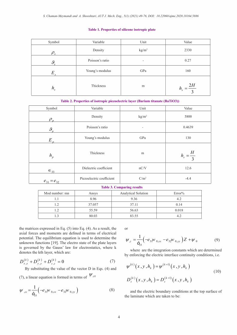
ValueUnitVariableSymbol

2330kg/m2Densitysρ

0.27-Poisson’s ratiosϑ

160GPaYoung’s modulussE

23sHh =mThickness

sh

ValueUnitVariableSymbol

5800kg/m2Densitypρ

0.4639-Poisson’s ratiopϑ

130GPaYoung’s moduluspE

3sHh =

mThicknessph

12.6nC/VDielectric coefficient33∈

-4.4C/m2Piezoelectric coefficient31 32e e=

Error%Analytical SolutionAnsysMod number: mn4.29.368.961.10.1437.1137.0571.20.01856.6355.591.24.283.5580.031.3

Table 1. Properties of silicone isotropic plate

Table 3. Comparing results

Table 2. Properties of isotropic piezoelectric layer (Barium titanate (BaTiO3))

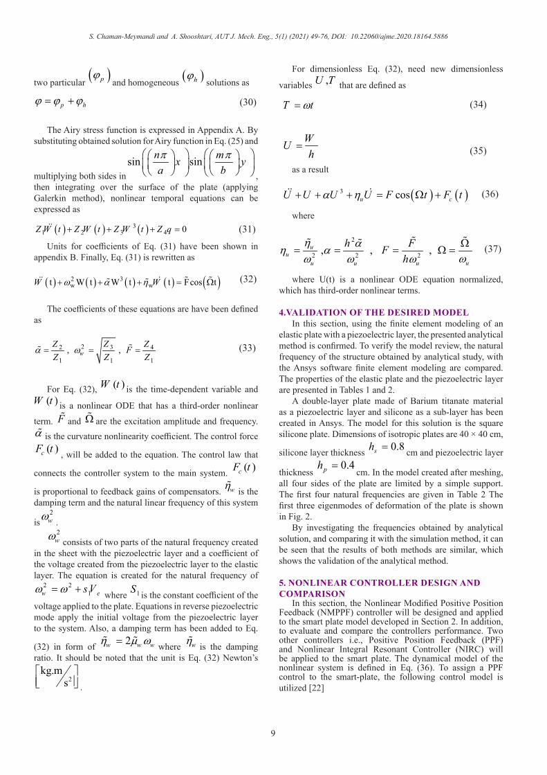
the matrices expressed in Eq. (5) into Eq. (4). As a result, the axial forces and moments are defined in terms of electrical potential. The equilibrium equation is used to determine the unknown functions [19]. The electro state of the plate layers is governed by the Gauss’ law for electrostatics, where k denotes the kth layer, which are:

(7) By substituting the value of the vector D in Eqs. (4) and

(7), a linear equation is formed in terms of ,zzψ

(8)

or

(9)

where are the integration constants which are determined by enforcing the electric interface continuity conditions, i.e.

(10)( ) ( ) ( ) ( )1, , , ,k k

k kx y h x y hψ ψ +=

( ) ( ) ( ) ( )1, , , ,k kz k z kD x y h D x y h+=

and the electric boundary conditions at the top surface of the laminate which are taken to be:

( ) ( ) ( ), , , 0k k k

x x y y z zD D D+ + =

( ), 31 0, 32 0,33

1 zz xx yye w e wψ = − −ò

( ), 31 0, 32 0, 033

1 z xx yye w e w Zψ ψ= − − +ò

5



6

Fig. 2. displacement plate in Ansys

Fig. 3. Time-domain diagram of the NMPPF and NIRC and PPF controlled system

7


(11)

3. EQUATIONS OF MOTIONUsing Hamilton’s principle, equations of motion of the

plate based on classical theory and von Karman strain–displacement relation can be obtained as [20]:

(12)

where q is the external excitation and ( 1, 2,3)iI i= =are the mass moment inertias and can be expressed as

(13)

where 2 ,I N is the rotational inertia and layer numbers. , , xx yy xyN N N

are in-plane forces , , xx yy xyM M M

are moments, which can be expressed as

(14)

(15)

Replacing Eqs. (2), (4) in Eqs. (14) and (15), the following relations are developed,

( ) , , 2hx y vψ =( ) , , 2 0 x y hψ − ⁄ =

2 20 0

0 12 2xyxx N u wN

I Ix y xt t

∂ ∂ ∂∂ ∂ + = − ∂ ∂ ∂∂ ∂

2 20 0

0 12 2xy yyN N v w

I Ix y yt t

∂ ∂ ∂ ∂ ∂+ = − ∂ ∂ ∂∂ ∂

( )

2 22

2 2

0 0 0 0

2 2 22 20 0 0 0 0

0 1 22 2 2 2 2

2

, ,

xy yyxx

xx xy xy yy

M MMx y xx y

w w w wN N N N

x y y x y

q x y t

w u v w wI I I

x yt t t x y

∂ ∂∂ ∂+ + +

∂ ∂ ∂∂ ∂

∂ ∂ ∂ ∂ ∂+ + + ∂ ∂ ∂ ∂ ∂

+

∂ ∂ ∂ ∂ ∂ ∂ ∂= + + − + ∂ ∂∂ ∂ ∂ ∂ ∂

10

11 2

2

1 k

k

N h

hk

II z dzI z

ρ+

=

=

∑∫

1

1

k

k

xx xxN h

yy yyhk

xy xy

NN dzN

σσσ

+

=

=

∑∫

1

1

k

k

xx xxN h

yy yyhk

xy xy

MM z dzM

σσσ

+

=

=

∑∫

(16)

(17)

where

(18)

(19)

The axial motions in x and y directions have been considered negligible and only transverse vibration has been

investigated; therefore, both in-pla)ne accelerations

20

2

vt

∂∂

and

20

2

ut

∂∂ can be ignored [21]. We also ignore rotational

inertia. Therefore, Eq. (12) can be rewritten as:

By introducing Airy stress functionϕ , in-plane relations can be defined as follows

011 12

012 22

066

111 12

112 22

166

00

0 0

00

0 0

xx xx

yy yy

xy xy

exx xx

eyy yy

exy xy

N A AN A AN A

B B NB B N

B N

εεε

εεε

=

+ −

011 12

012 22

066

111 12

112 22

166

00

0 0

00

0 0

xx xx

yy yy

xy xy

exx xx

eyy yy

exy xy

M B BM B BM B

D D MD D M

D M

εεε

εεε

=

+ −

( ) [ ]( )22

1 2

, , 1, , hN

ij ij ij hk

A B D Q z z dz−=

=∑∫

( )[ ] 2

1 2

, 1,hN

e eh

k

N M z e E dz−=

= ∑∫

( )

02 22

2 20

200

2 2 20

0 22 2 20 0

2

0, 0

2

, ,

xy xy yyxx

xxxy yyxx

xy

xy

yy

N N NNx y x y

wNM MM x

wx y x yx y Ny

wwN

wx xq x y t I Iw t t wNy y

∂ ∂ ∂∂+ = + =

∂ ∂ ∂ ∂

∂ + ∂ ∂∂ ∂ ∂∂ + + + +

∂ ∂ ∂ ∂ ∂∂ ∂ ∂

∂∂ + ∂ ∂∂ ∂ + = − ∂ ∂ ∂ ∂+ ∂ ∂

(20)


8

(21)

Presented relations in Eq. (21) satisfy the first two conditions of Eq. (20). Airy function can be determined using the following compatibility condition:

(22)

Also, Eq. (16) can be rewritten as:

(23)

where

(24)

Substituting Eqs. (17), (21), (23) and (24) in Eqs. (20) and (22),

(25)

2

2

2

2

2

xx

yy

xy

Ny

Nx

Nx y

ϕ

ϕ

ϕ

∂= ∂

∂ =∂

∂= − ∂ ∂

[ ]* 1

* 13*3

* 1

0A A

B A B OD D BA B

−

−

−

= = − = = = −

( ) ( )* * *

0 3*3

1* * *3*3

T T

e

e

A B A ON

M B D B I

N

M

εε

= + − − −

22 0 2 0 22 00

2 2

2 20 0

2 2

yy xy xx wx y x yx y

w wx y

ε ε ε ∂ ∂ ∂∂− + = ∂ ∂ ∂ ∂∂ ∂

∂ ∂−∂ ∂

( )

2 1 2 12 1 2 1

11 12 12 222 2 2 2

2 1 2 22 20 0

66 2 2

2 22 20 0

2 2

2 22 20 0

0 22 2 2 2

2

, ,

0

yy yyxx xx

xy

D D D Dx x y y

w wD

x y x y x yy x

w wq x y t

x y x y x y

w wwI It t x y

ε εε ε

ε ϕ ϕ

ϕ ϕ

∂ ∂∂ ∂+ + +

∂ ∂ ∂ ∂

∂ ∂ ∂∂ ∂ + + − ∂ ∂ ∂ ∂ ∂ ∂∂ ∂ ∂ ∂∂ ∂

+ − + + ∂ ∂ ∂ ∂ ∂ ∂ ∂ ∂∂ ∂

= − + ∂ ∂ ∂ ∂

(26)

By substituting obtained equation for ϕ from Eq. (26) in

Eq. (25), a nonlinear equation for transverse plane vibrations is obtained. A boundary condition is required to solve Eq. (24). It is required to determine the boundary conditions of the problem to derive Erie’s stress function and the plate transverse deformation. Here, boundary conditions are considered as a simple support. Therefore,

(27)

According to the boundary conditions 0w can be defined as Equation (28):

(28)

where m and n refer to the vibrational mode number

and the time variable ( )mnW t related to the transverse deformation. According to Eq. (3), Eq. (28) can be rewritten

for 0u and 0v as

(29)

Substituting Eq. (28) in Eq. (26) and using boundary

conditions of Eq. (29), Airy function can be determined by

2 2* * *2 11 12 112 2

2*12

2 2* * *2 12 22 122 2

2*22

22 2 22 2* 0 0 066 2 2

2

exx

eyy

exx

eyy

A A A Ny x

yA N

A A A Ny x

xA N

w w wA

x y x y x y y x

ϕ ϕ

ϕ ϕ

ϕ

∂ ∂+ + ∂ ∂ ∂

∂ + ∂ ∂

+ + ∂ ∂ ∂+ ∂ +

∂ ∂ ∂∂ ∂+ = − ∂ ∂ ∂ ∂ ∂ ∂ ∂ ∂

0 0 0 0,xx xyw v M N at x a= = = = =

0 0 0 0,yy xyw u M N at x a= = = = =

20 0

0 0

1 0, 0,2

a

xxw

u dx at y bx

ε∂ = − = = ∂ ∫

20 0

0 0

1 0, 0,2

b

yyw

v dy at x ax

ε∂ = − = = ∂ ∫

00 0,

b

xyN dy at x a= =∫

00 0,

a

xyN dx at y b= =∫

( ) ( ) ( )

( )

01 1

1 1

, , ,

mnn m

mnn m

w x y t W t F x y

n x m yW t sin sina bπ π

∞ ∞

= =∞ ∞

= =

= =

∑∑

∑∑

9


two particular ( )pϕ and homogeneous ( )hϕ solutions as

(30)

The Airy stress function is expressed in Appendix A. By substituting obtained solution for Airy function in Eq. (25) and

multiplying both sides insin sinn mx y

a bπ π

,

then integrating over the surface of the plate (applying Galerkin method), nonlinear temporal equations can be expressed as

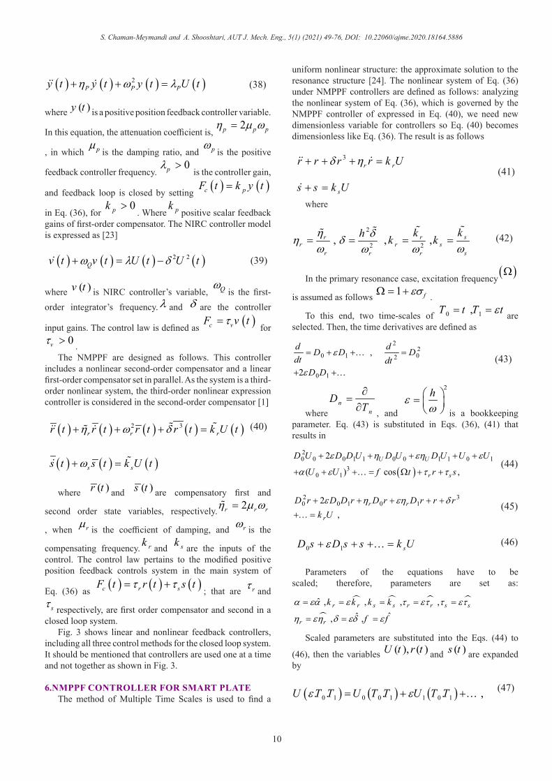
(31) Units for coefficients of Eq. (31) have been shown in

appendix B. Finally, Eq. (31) is rewritten as

(32)

The coefficients of these equations are have been defined as

(33)

For Eq. (32), ( )W t is the time-dependent variable and ( )W t is a nonlinear ODE that has a third-order nonlinear

term. F and Ω are the excitation amplitude and frequency. α is the curvature nonlinearity coefficient. The control force

( )cF t , will be added to the equation. The control law that

connects the controller system to the main system. ( )cF t

is proportional to feedback gains of compensators. wη is the damping term and the natural linear frequency of this system

is2

wω .2

wω consists of two parts of the natural frequency created in the sheet with the piezoelectric layer and a coefficient of the voltage created from the piezoelectric layer to the elastic layer. The equation is created for the natural frequency of

2 21w es Vω ω= + where 1S is the constant coefficient of the

voltage applied to the plate. Equations in reverse piezoelectric mode apply the initial voltage from the piezoelectric layer to the system. Also, a damping term has been added to Eq.

(32) in form of 2w w wη µ ω= where wη is the damping ratio. It should be noted that the unit is Eq. (32) Newton’s

2kg.m

s .

p hϕ ϕ ϕ= +

( ) ( ) ( )31 2 3 4 0Z ZW t Z W t Z W t q+ + + =

( ) ( ) ( ) ( ) ( )2 3w wt W t W t t Fcos tW Wω α η+ + + = Ω

2 32 4

1 1 1 , , w

ZZ ZFZ Z Z

α ω= = =

For dimensionless Eq. (32), need new dimensionless

variables ,U T that are defined as

(34)T tω=

(35)WUh

=

as a result

( ) ( )3 cosu cU U U F t F tU α η+ + + = Ω +

(36)

where

(37)

where U(t) is a nonlinear ODE equation normalized,

which has third-order nonlinear terms.

4.VALIDATION OF THE DESIRED MODELIn this section, using the finite element modeling of an

elastic plate with a piezoelectric layer, the presented analytical method is confirmed. To verify the model review, the natural frequency of the structure obtained by analytical study, with the Ansys software finite element modeling are compared. The properties of the elastic plate and the piezoelectric layer are presented in Tables 1 and 2.

A double-layer plate made of Barium titanate material as a piezoelectric layer and silicone as a sub-layer has been created in Ansys. The model for this solution is the square silicone plate. Dimensions of isotropic plates are 40 × 40 cm,

silicone layer thickness 0.8sh = cm and piezoelectric layer

thickness 0.4ph =

cm. In the model created after meshing, all four sides of the plate are limited by a simple support. The first four natural frequencies are given in Table 2 The first three eigenmodes of deformation of the plate is shown in Fig. 2.

By investigating the frequencies obtained by analytical solution, and comparing it with the simulation method, it can be seen that the results of both methods are similar, which shows the validation of the analytical method.

5. NONLINEAR CONTROLLER DESIGN AND COMPARISON

In this section, the Nonlinear Modified Positive Position Feedback (NMPPF) controller will be designed and applied to the smart plate model developed in Section 2. In addition, to evaluate and compare the controllers performance. Two other controllers i.e., Positive Position Feedback (PPF) and Nonlinear Integral Resonant Controller (NIRC) will be applied to the smart plate. The dynamical model of the nonlinear system is defined in Eq. (36). To assign a PPF control to the smart-plate, the following control model is utilized [22]

2

2 2 2 , , , uu

uu u u

h FFh

η αη αωω ω ωΩ

= = = Ω =


10

(38)

where ( )y t is a positive position feedback controller variable.

In this equation, the attenuation coefficient is, 2p p pη µ ω=

, in which pµ is the damping ratio, and pωis the positive

feedback controller frequency. 0pλ >

is the controller gain,

and feedback loop is closed by setting ( ) ( )c pF t k y t=

in Eq. (36), for 0pk >

. Where pkpositive scalar feedback

gains of first-order compensator. The NIRC controller model is expressed as [23]

(39)( ) ( ) ( ) ( )2 2Qv t v t U t U tω λ δ+ = −

where ( )v t is NIRC controller’s variable, Qω is the first-order integrator’s frequency.λ and δ are the controller

input gains. The control law is defined as ( )c vF v tτ= for

0vτ > . The NMPPF are designed as follows. This controller

includes a nonlinear second-order compensator and a linear first-order compensator set in parallel. As the system is a third-order nonlinear system, the third-order nonlinear expression controller is considered in the second-order compensator [1]

(40)( ) ( ) ( ) ( ) ( )2 3r r rt t r t r t k U tr rη ω δ+ + + =

( ) ( ) ( )s ss t s t k U tω+ =

where ( )r t and ( )s t are compensatory first and

second order state variables, respectively. 2r r rη µ ω=

, when rµ is the coefficient of damping, and rω is the

compensating frequency. rk and sk are the inputs of the control. The control law pertains to the modified positive position feedback controls system in the main system of

Eq. (36) as ( ) ( ) ( )c r sF t r t s tτ τ= +; that are rτ and

sτ respectively, are first order compensator and second in a closed loop system.

Fig. 3 shows linear and nonlinear feedback controllers, including all three control methods for the closed loop system. It should be mentioned that controllers are used one at a time and not together as shown in Fig. 3.

6.NMPPF CONTROLLER FOR SMART PLATEThe method of Multiple Time Scales is used to find a

uniform nonlinear structure: the approximate solution to the resonance structure [24]. The nonlinear system of Eq. (36) under NMPPF controllers are defined as follows: analyzing the nonlinear system of Eq. (36), which is governed by the NMPPF controller of expressed in Eq. (40), we need new dimensionless variable for controllers so Eq. (40) becomes dimensionless like Eq. (36). The result is as follows

(41)3

r rr r r r k Uδ η+ + + =

ss s k U+ = where

(42)

In the primary resonance case, excitation frequency ( )Ω

is assumed as follows 1 fεσΩ = + .

To this end, two time-scales of 0 1 , T t T tε= = are selected. Then, the time derivatives are defined as

(43)

wheren

n

DT∂

=∂ , and

2hεω = is a bookkeeping

parameter. Eq. (43) is substituted in Eqs. (36), (41) that results in

(44)

(45)

(46)0 1 sD s D s s k Uε+ + +…=

Parameters of the equations have to be scaled; therefore, parameters are set as:

Scaled parameters are substituted into the Eqs. (44) to

(46), then the variables ( ), ( )U t r t and ( )s t are expanded by

(47)

2

2 2 , , , sr rr r s

r sr r

kkh k kη δη δω ωω ω

= = = =

( )

20 0 0 1 1 0 0 1 1 0 1

30 1

2

( ) cos ,U U

r s

D U D D U D U D U U U

U U f t r s

ε η εη ε

α ε τ τ

+ + + + +

+ + +…= Ω + +

22

0 1 02

0 1

,

2

d dD D Ddt dt

D D

ε

ε

= + +… =

+ +…

2 30 0 1 0 1 2

,r r

r

D r D D r D r D r r rk Uε η εη δ+ + + + +

+…=

, , , ˆ ,

, ˆˆ , r r s s r r s s

r r

k k k k

f f

α εα ε τ ετ τ ετ

η εη δ εδ ε

= = = = =

= = =

( ) ( ) ( )0 1 0 0 1 1 0 1. . . . ,U T T U T T U T Tε ε= + +…

( ) ( ) ( ) ( )2P P Py t y t y t U tη ω λ+ + =

11


uniform nonlinear structure: the approximate solution to the resonance structure [24]. The nonlinear system of Eq. (36) under NMPPF controllers are defined as follows: analyzing the nonlinear system of Eq. (36), which is governed by the NMPPF controller of expressed in Eq. (40), we need new dimensionless variable for controllers so Eq. (40) becomes dimensionless like Eq. (36). The result is as follows

(41)3

r rr r r r k Uδ η+ + + =

ss s k U+ = where

(42)

In the primary resonance case, excitation frequency ( )Ω

is assumed as follows 1 fεσΩ = + .

To this end, two time-scales of 0 1 , T t T tε= = are selected. Then, the time derivatives are defined as

(43)

wheren

n

DT∂

=∂ , and


parameter. Eq. (43) is substituted in Eqs. (36), (41) that results in

(44)

(45)

(46)0 1 sD s D s s k Uε+ + +…=


Scaled parameters are substituted into the Eqs. (44) to

(46), then the variables ( ), ( )U t r t and ( )s t are expanded by

(47)

(48)( ) ( ) ( )0 1 0 0 1 1 0 1. . . .r T T r T T r T Tε ε= + +… ,

(49)( ) ( ) ( )20 1 0 0 1 1 0 1. . . . .s T T s T T s T Tε ε ε= + +…

By placing Eqs. (44), (45) and (46) in Eqs. (47), (48) and

(49) and ordering the result in terms of the power of0ε ,

1ε

and2ε , the following differential equations are obtained.

(50)( )0 20 0 0: 0 ,O D U Uε + =

(51)

(52)

(53)

(54)

(55)( )20 1 1 1 1 0: ˆ ,sO D s s k U D sε + = +

The order

2ε is considered for s only as function based on

Eq. (49) includes the orders of 1ε and

2ε .

(56)( ) 00 1 ,iTU A T e cc= +

(57)( ) 00 1 ,iTr B T e cc= +

Thus, 1 1( ), ( )A T B T are complex parameters functions that will be defined by deface the secular terms, also where

0U domain is 0r , which is a function of function 1T .

(58)

Thus, 1( )C T is obtained in the next steps. At this step, Eqs. (56) to (58) are inserted into Eqs. (52), (53): Ultimately, the results are simplified as follows.

( ) ( ) ( )0 00 1 11

ˆ

2iT iTsk

s C T e i A T e cc= + − +

20 0 0 0 D r r+ =

( ) ( )1 20 1 1 0 0

30 1 0 0 0 0

:

2 ,

ˆ ˆ ˆ

ˆ ˆr s

u

O D U U fcos t r s

D D U D U U

ε τ τ

η α

+ = Ω + +

− − −

20 1 1 0 0 1 0

30 0 0

2

.

ˆ

ˆˆr

r

D r r k U D D r

D r rη δ

+ = −

− −

0 0 0 0 ˆsD s s k U+ =

(59)

(60)

1U and 1r are calculated using Eqs. (59) and (60) in time

domain. Eq. (58) and 1U have been substituted in Eq. (55) for creating ODE equations to solve the equation. Moreover, the term cc shows the complex conjugate function of its preceding sentences.

For the system to have a bounded solution, it must be considered zero to the secular terms. Applying this condition

to the expanded Eq. (55) and using 1U , 1( )C T is calculated as

(61)( )1

ˆ2

1

ˆ

s sk

T

sC T c eτ

=

where sc is a constant. Next step is to sort Eqs. (59) and (60), and separate the secular terms,

(62)

(63)

The solution to Eqs. (62) and (63) is assumed in the polar form of

(64)( ) ( ) ( )11 1

1 ,2

ai TA T a T e ζ=

( ) ( ) ( )( )

( ) ( ) ( )

( )

0

0 0 0

0 0 0

20 1 1 1 1 1 1

1 1

33 21

ˆ

ˆˆ

ˆ

ˆ

ˆˆ

2

1 2

32

iTr u

iT T iTss

i T iT i T

D U U B T e A T D A T

kie C T e i A T e

fA T e A Ae e cc

τ η

τ

α α

−

Ω

+ = − +

+ + −

− − + +

( ) ( )( ) ( ) ( )( )

0 0

0 0

32 30 1 1 1 1

21 1 1 1

3 ˆ

ˆ ˆ

ˆ 2

iT i Tr

iT iTr

D r r k A T e B T e

B B T e B T D B T ie

δ

δ η

+ = −

− − +

( )

( ) ( )

( ) ( )( )

( ) ( )

1

0

1

1

1

1 1 1

21 1

2 0 ,2

32

ˆˆˆ

ˆ

ˆˆ

r

f

i Tr

s ss

iT

u

i T

B T e

k i A Te

A T D A T i

f e A T A T

σ

σ

τ

τ ω

η

α

+

− =− + + −

( ) ( ) ( )( ) ( )( )

0

21 1 1

1 1 1

3 0,

ˆ 2

ˆ ˆr r

r

i Tr i T

r

k A T e B T B Te

B T D B T i

σω

δ

η

− − =− +


12

Variable αValue 11.7 0.03 9.36

Variablepλ pk

pµ pω FValue 1 1 0.002 9.36 0.09

Table 4. Numerical values of the main system parameters

Fig. 4. Frequency response of the uncontrolled system

Table 5. Numerical values of the PPF controller parameters

uµ uω

13


Fig. 5. Frequency response of the PPF controlled


14

Fig. 6. Sensitivity analysis of the closed-loop PPF controlled system to control parameters. (a) damping coefficient ( )rµ , (b) control gain ( )pλ , (c) control gain ( )pk , (d) voltage ( )V

(c)

(a) (b)

(d)

15


(65)( ) ( ) ( )11 1

1 ,2

bi TB T b T e ζ=

The real and imaginary parts will be separated and equal to zero by placing Eqs. (64) and (65) in Eqs. (62) and (63) The following equations are obtained.

(66)

(67)

(68)

(69)

Since all variables of Eqs. (66) to (66) are time derivatives

of 1T function. New variables are defined, as follows to obtain the set of independent equation

. by applying these changes, the modulation equation is obtained as follows.

(70)

(71)

( ) ( ) ( )

( ) ( ) ( )( )

( )

11 1 1

1

1 1 1 1

1

ˆ ˆˆ

sin2 2

sin2

2

ˆ

ˆ

fs s

a

rr b a

u

Tk fD a T a TT

b T T T T

a T

στζ

τ σ ζ ζ

η

= − + −

+ + −

−

( ) ( ) ( )( )( )

( )( )

( ) ( )( )

121 1 1

1 1

1 11

1 1

3 cos 8 2

cos

ˆ

2

ˆ

ˆˆ ˆ2

fa

a

r br s s

a

TfD T a Ta T T

T Tb T ka T T

σαζζ

σ ζτ τζ

= − −

+ − − −

( ) ( )

( ) ( ) ( )( )( )1 1 1

1 1 1 1

i

ˆˆ2 2

s n

r r

a r b

kD b T b T a

T T T T

η

ζ σ ζ

= − +

− −

( ) ( ) ( )( )

( ) ( )( )( )

121 1 1

1

1 1 1

3 8 2

cos

ˆˆr

b

a r b

k a TD T b T

b T

T T T

δζ

ζ σ ζ

= − +

− −

( ) ( ) ( ) ( ) ( ) and a f a b r b at t t t t t tθ σ ζ θ σ ζ ζ= − = + −

( ) ( )

2 2

sin sin2 2

ˆˆ ˆ

ˆ ˆ

u s s

ra a

ka a

f b

η τ

τθ θ

= − + +

+

(72)( )ˆˆ

sin2 2r r

bk

b b aη

θ= − −

(73)

steady-state conditions are considered to obtain the

frequency response of the closed loop system. The coupled equations obtained for the frequency are the response of the main system and the controller domain.

(74)

(75)

7. RESULTS AND DISCUSSIONSThis part has discussed the vibration range in the resonant

frequency region and the performance of the controllers in controlling the vibration amplitude in the resonance region are discussed and its details.

7.1. Open-Loop System Response Under Primary ResonanceIt is necessary to provide an image of the system reaction

in an uncontrolled mode prior to studying the closed loop system. The open-loop system is obtained from Eqs. (74) and (75). The values of the main system are given in Table 4 and the frequency response graph in Fig. 4. System behavior is defined for the excitation force 0.09f = [N]. The jump phenomenon is seen in the excitation range. The purpose of the controllers is to diminish the maximum vibration range in the frequency domain. Using analytical relations and structural dimensions simulated in Ansys, the values of the desired parameters are obtained.

7.2. Ppf Controller Performance AnalysisThis part examined the performance of the closed loop

system with PPF controller [1,22]. The equations of the PPF controller frequency response equations are shown as the NMPPF controller by the multiple time scale approach. These equations are obtained by forms Eqs. (76) and (77). Fig. 5

( ) ( )

2

c

ˆˆ38 2

1 os cos2

ˆ

ˆ2

ˆ

s sa

ra b f

ka

f ba a

ταθ

τθ θ σ

= − + +

+ +

( )

( )

2

2

3 1 cos8 2

3cos2 2

ˆˆ

ˆˆ ˆˆ8ˆ

2

b a

s sr rb r

fba

kb k aa

a b

δθ θ

ττ αθ σ

= + +

− − + +

( )

22 2

24

3

2

2 2 2 2

338

ˆˆ ˆ ˆˆ ˆ

ˆ ˆˆ ˆ ˆˆ8 ˆ2 ˆ

u s s r r

r

s s r r

r r

r f f

k bf ak a

k ba aak k

b aa

η τ τ η

τ δτ τα

σ σ σ

= + +

+ − −

+ − −

( )1

2 2 32

22

3 21 .ˆˆ

ˆ ˆ4 ˆr

r fr r r

b b ba aak k k

η δ σ σ − = + −


16

Fig. 7. Frequency response of the NIRC controlled

Fig. 8. NIRC controlled system response for changes in excitation amplitude. (a) controller input gain ( )λ , (b) controller input gains ( )τ .

(b)(a)

17


Variable

rτ

sk sτ

Value 9.36 9.36 0.002 0 2 1 2 1 0.09

f

Fig. 9. The effect of the voltage on the NIRC

Table 7. Numerical values of the NMPPF controller

Table 6. Numerical values of the NIRC controller parameters

Variablef

Value 9.36 2 0 1 0.09

Qω λ δ vτ

rω sω rµ δ rk


18

Fig. 11. Frequency response of the closed-loop system for values of damping ratio

Fig. 10. Frequency response of the NMPPF controlled system

19


Fig. 12. Sensitivity of the closed-loop NMPPF controlled system response. (a) controller input gain for the second order ( )rk , (b) gain for the second order compensator ( )rτ , (c) controller input gain for the first order ( )sk , (d) gain for

the first order compensator ( )sτ

(a)

(d)(c)

(b)


20

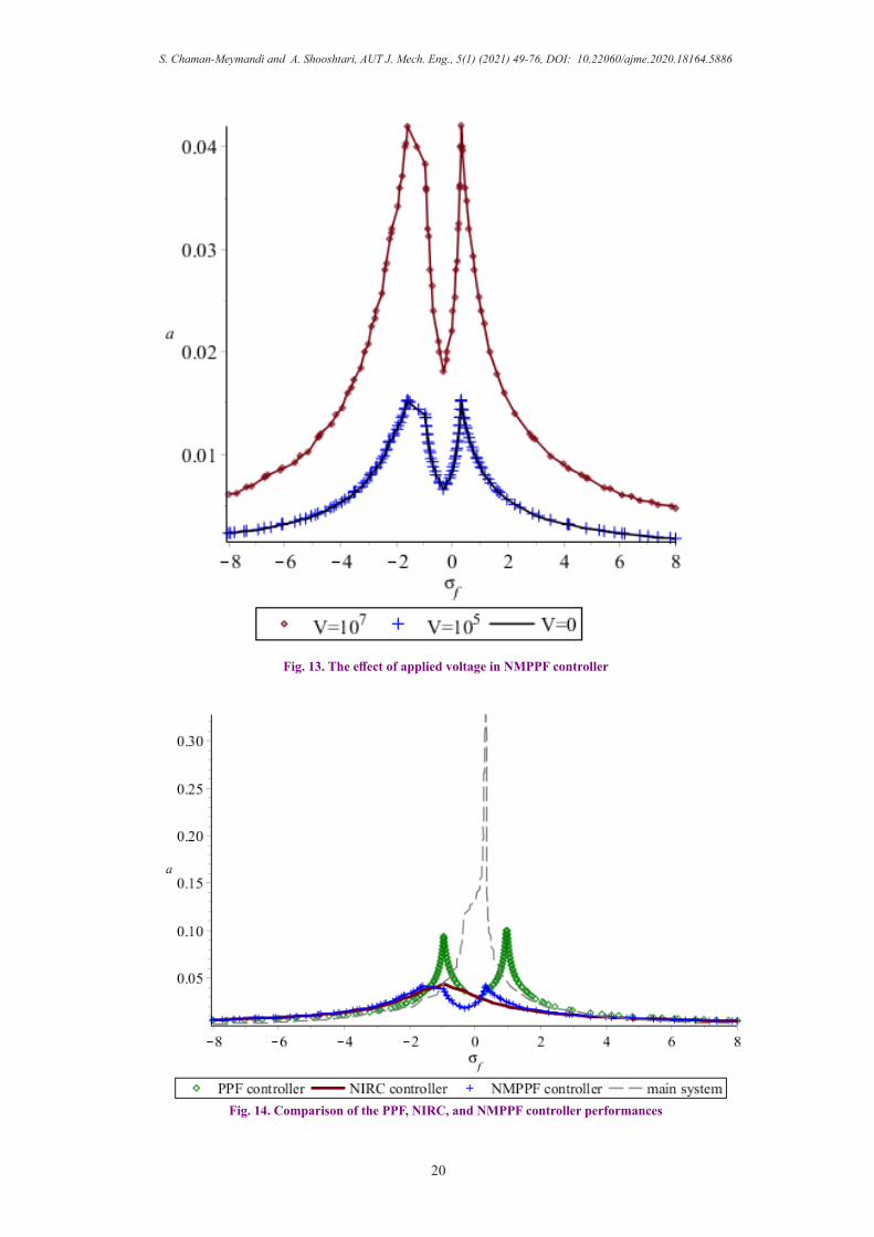
Fig. 13. The effect of applied voltage in NMPPF controller

Fig. 14. Comparison of the PPF, NIRC, and NMPPF controller performances

21


Controller Amplitude Improved performance compared to the main system

Main system 0.325 --NMPPF 0.042 87.08%

PPF 0.10 69.23%NIRC 0.044 86.46%

indicates the frequency response of the closed loop system with the PPF controller. The controller parameters are cited in Table 5. Implementation of PPF controller reduces vibration

range in the resonant frequency region ( )0fσ =. This

controller amplifies the production of two-peak amplitudes with relatively large amplitude around the frequency. The amplitude in the resonant frequency reduced from 0.32a = to 0.1a = in the uncontrolled mode. Thus, one can state that it is suitable for controlling vibrations at resonant frequency, although it does not perform well around resonant frequency. The frequency response equations are as follows

(76)

(77)

An analysis of each control parameter is done for obtaining

a better understanding of the effect of each parameter in response to improved system performance. The

PPF controller is suitable for controlling the excitation

amplitude at ( )0fσ =. However, as shown in Figs. 5 and

6, the amplitude of the resonator is practically converted to two frequencies near the natural frequency (before and after) by applying this controller. Fig. 6 indicates the sensitivity of the amplitude response to changes in control parameters. Fig. 6(a) as the coefficient of damping increases, the amplitude of the vibrations decreases almost linearly. The controller input gain results indicated in Figs. 6(b) and 6(c) have similar effects. Increasing these parameters ends in more inhibition of the precise frequency value of the resonator. Although by increasing these two parameters the two peaks are separated, it is impossible to comment on the two peaks created. Fig.

6(c) shows that the controller behavior changes when1pλ =

. As is seen in Fig. 6(d), the voltage change has a direct effect

on the amplitude of the resonator. By affecting the frequency, this parameter changes the other parameters. The following figure shows the increase in voltage that decreases the amplitude of the vibrations.

The analytical solution of this controller is given in Appendix C.7.3. Nirc Controller Performance Analysis

In this section, the outcomes of applying NIRC control method on the smart plate is discussed. The NIRC consists of a first-order resonant integrator that provides additional damping in a closed-loop system response to reduce high amplitude nonlinear vibration around the fundamental resonance frequency. Numerical values of the NIRC controller are listed in Table 6. Fig. 7 shows the steady-state vibration amplitude versus changes in excitation frequency. Unlike conventional methods such as PPF and NMPPF, the graph shows small bending toward the negative side of the frequency axis. The NIRC controlled system exhibits no high-amplitude peak on either side of the fundamental mode in the frequency domain. Fig. 7 is obtained from the analytical solution Method of Multiple Scales such as the solution NMPPF. Next, the effects of three control variables on system response are examined. Fig. 8 shows the vibration amplitude of an NIRC controlled smart plate when control parameters are changed.

(78)

According to Fig. 8(a) increasing the positive values input gain controller λ , reduce domains. Negative values of this parameter causes the graph to bend to the right. In addition, reducing the negative values of the input gain λ will increase the vibration suppression. Fig. 8(b) shows the closed loop response of the system based on the variations in the input gain parameter,τ . Results demonstrate that as expected both gains have similar effect on the response. However, better suppression is achieved when both gains have the same signs. Fig. 9 shows the effect of the voltage on the amplitude of vibrations. As expected, increasing the voltage increases the amplitude of vibrations. The analytical solution of this controller is given in Appendix D.

Table 8. Comparison of values and percentages the PPF, NIRC, and NMPPF controller performances

( )

22 2

22

3

ˆ

2

ˆ

2 2

ˆ38

ˆ ˆˆ

ˆ

p pu

p

pf f

p

k bf aa

k ba aa

ηηλ

α σ σλ

= + +

− −

( )

12 22

22

2 1ˆˆ ˆ

pf

p p

b baa

ησ

λ λ

− =

23

2

2

34

2

ˆˆ

2ˆ

2

vu

vf

aaf a

a

αλ τη

λτ σ

− = + + +


22

7.4. Nmppf Controller Performance AnalysisModulation Eqs. (74) and (75) were used to show the

performance of the NMPPF controller on the smart plate. The numerical values of the parameters are selected in accordance with Table 7 for NMPPF controller. Fig. 10 shows the frequency response of NMPPF controlled systems. In this Fig., the right peak has higher amplitude than the left peak, but does not skip the amplitude.

By using this method not only the vibration reduces at the resonant frequency, but also the other two peaks have less amplitude than the PPF method. The maximum amplitude in NMPPF controlled system is much lower than the maximum peak in the controlled PPF response. NMPPF controller parameters, attenuation ratio and compensating frequencies, affect the closed loop system inhibition performance.

Moreover, the four control responses change the system response in the control process. Here the effect of these parameters on the system response is examined. The first

parameter examined is rµ . According to Fig. 11, the changes

in parameter rµ in the controller are such that with increase in its value, vibrations amplitude decreases. In the next step, the other benefits of the controller are examined.

Fig. 12 shows the second-order input variable rk

, the second-order output value rτ , the first-order input

compensator variable sk , and the first-order output

compensator interest sτ . According to Fig. 12(a), the increase

in rk does not decrease the value of two peaks in the system

response but makes them distance. Moreover, small rk values do not reduce the magnitude of the two peak values.

Nonetheless, with increase in rk , the amplitude of the

vibrations at the resonant frequency ( )0fσ =improves.

As the second-order output rτ increases in Fig. 12(b), the amplitude in the resonance frequency region decreases as a result of the inhibition of the vibration amplitude at frequency as Fig. 12(b) shows. Moreover, the two peak values occur at distances beyond the origin as the graphs become wider in the frequency range. Fig. 12(c) and Fig. 12(d) show the effect

of first-order compensatory interest changes, sk and sτ As already stated, second-order compensators have a better impact on amplification amplitude compared to second-order

compensator diagrams. The increase in sk increases the level of control of the controller that decreases the amplitude of

the vibrations. The control gain function sτ decreases with increase in parametric value of the system domain and the

two peaks get distant like sk .

Finally, evaluating the effect of voltage applied to the plate in the NMPPF controller, it is observed that increasing the voltage increases the amplitude of response.

Fig. 14 shows the frequency response of the uncontrolled system, system with PPF, NIRC, and NMPPF controllers for the excitation amplitude of 0.09f = . NPPF and NIRC controllers have a nearly similar effect on reducing amplitude at the resonant frequency. The PPF controller has a weaker performance than the other two controllers.

Appendix AAiry functionwhere particular solution is considered as

(A-1)

(A-2)

( ) ( )2 2 2

21 12 2 *

22

. 32

mnmn

a m W tW t

b n Aϕ ϕ= =

( ) ( )2 2 2

22 22 2 *

11

. 32

mnmn

b n W tW t

a m Aϕ ϕ= =

3 0ϕ = A homogeneous solution form can be considered as

2 21 2 3h C x C y C xyϕ = + +

Appendix BThe units in Table 9 are the coefficients of Eq. (31). These

1 2

3

2 2cos cospn x m ya b

n x m ysin sina b

π πϕ ϕ ϕ

π πϕ

= +

+

( )

2 22* *

1 12 11

1* * * 211 22 12

16

2

mn

eyy

W n mC A Aa b

NA A A

π π

−

= − −

− −

( )

2 22* *

2 22 12

1* * * 211 22 12

16

2

mn

exx

W n mC A Aa b

NA A A

π π

−

= −

− −

3 0C =

(A-3)

(A-4)

23


Finally, evaluating the effect of voltage applied to the plate in the NMPPF controller, it is observed that increasing the voltage increases the amplitude of response.

Fig. 14 shows the frequency response of the uncontrolled system, system with PPF, NIRC, and NMPPF controllers for the excitation amplitude of 0.09f = . NPPF and NIRC controllers have a nearly similar effect on reducing amplitude at the resonant frequency. The PPF controller has a weaker performance than the other two controllers.

Appendix AAiry functionwhere particular solution is considered as

(A-1)

(A-2)

( ) ( )2 2 2

21 12 2 *

22

. 32

mnmn

a m W tW t

b n Aϕ ϕ= =

( ) ( )2 2 2

22 22 2 *

11

. 32

mnmn

b n W tW t

a m Aϕ ϕ= =

3 0ϕ = A homogeneous solution form can be considered as

2 21 2 3h C x C y C xyϕ = + +

Appendix BThe units in Table 9 are the coefficients of Eq. (31). These

units are in Newton SI version and lead to the unit kg m/s2.Appendix C

Analytical solution of the controller PPFwe need new dimensionless variable for controllers so Eq.

(38) becomes dimensionless like Eq. (36). The result is as follows

where

(C-1)

To this end, two time-scales of 0 1,T t T tε= = are selected. Then, the time derivatives are defined as

(C-2)

where n

n

DT∂

=∂ and


parameter. Eq. (C-2) is substituted in equation main system and controller that results in

(C-3)

(C-4)


(C-5)

Scaled parameters are substituted into the Eqs. (C-3), (C-

4), then the variables ( ), ( )U t y t are expanded by

(C-6)( ) ( ) ( )0 1 0 0 1 1 0 1. . . . ,U T T U T T U T Tε ε= + +…

(C-7)( ) ( ) ( )0 1 0 0 1 1 0 1, , , ,y T T y T T y T Tε ε= + +…

ConstantUnit [M] [MT-2] [ML-2T-2] [MLT-2]

, ˆ ˆˆ, , ,ˆ p p p p p pk k f fα εα λ ελ ε η εη ε= = = = =

2 ˆ

, prp p

r p

kηη λ

ω ω= =

By placing above equations ordering the result in terms

of the power of 0 1,ε ε and

2ε , the following differential equations are obtained

(C-8)( )0 20 0 0: 0 ,O D U Uε + =

(C-9)

(C-10)

(C-11)20 1 1 0 0 1 0 0 0 2 ,ˆ ˆp rD y y U D D y D yλ η+ = − −

The equations of (C-8) and (C-9) are expressed as follows.

(C-12)( ) 00 1 ,iTU A T e cc= +

(C-13)( ) 00 1 ,iTy B T e cc= +

where 1( )A T and 1( )B T are complex parameters functions that will be defined by deface the secular terms,

also where 0U domain is 0r , which is a function of function

. Moreover, the term cc shows the complex conjugate function of its preceding sentences.

Next, Eqs. (C-12), (C-13) are substituted into the Eqs. (C-10) to (C-11). The simplified result is:

(C-14)

(C-15)

2

0 1 2

20 0 1

,

2

d dD Ddt dtD D D

ε

ε

= + +… =

+ +…

( )

20 0 0 1 1 0 0

31 1 0 1 0 1

2

( ) cos ,

U

U

r s

D U D D U D U

D U U U U Uf t r s

ε η

εη ε α ετ τ

+ + +

+ + + + +…

= Ω + +20 0 1 0

1

ˆ

2 p

p p

D y D D y D y

D y y U

ε η

εη λ

+ + +

+ +…=

( ) ( )1 20 1 1 0

30 1 0 0 0 0ˆ

:

2 ,

ˆ ˆ

ˆp

u

O D U U fcos t k y

D D U D U U

ε

η α

+ = Ω +

− − −

( )( )( )

( )

0

0 0 0

0

120 1 1 1

1 1

33 21

2

3

2

ˆˆ

ˆ ˆˆ

uiTp

iT i T iT

i T

A TD U U k B T e

D A T

ie A T e A Ae

f e cc

η

α α

Ω

+ + = −

− −

+ +

( )( ) ( )( )

0

0

20 1 1 1

1 1 1

ˆ

2ˆ

iTp

iTp

D y y A T e

B T D B T ie

λ

η

+ =

− +

Table 9. The units of the coefficients of transverse equation of the plate.

20 0 0 0 ,D y y+ =

1Z 2Z 3Z 4Z


24

1U and 1y are calculated using Eqs. (C-14) and (C-15) in time domain. For the system to have a bounded solution, it must be considered zero to the secular terms.

Next step is to sort Eqs. (C-14) and (C-15), and separate the secular terms,

(C-16)

(C-17)

The solution to Eqs. (C-16) and (C-17) is assumed in the polar form of

(C-18)( ) ( ) ( )11 1

1 ,2

ai TA T a T e ζ=

(C-19)( ) ( ) ( )11 1

12

bi TB T b T e ζ=

The real and imaginary parts will be separated and equal to zero by placing Eqs. (C-18) and (C-19) in Eqs. (C-16) and (C-17) The following equations are obtained.

(C-20)

(C-21)

(C-22)

(C-23)

Since all variables of Eqs. (C-20) to (C-23) are time derivatives of function. New variables are defined, as follows to obtain the set of independent equations:

. by applying these changes, the modulation equation is obtained as follows.

(C-24)( ) ( )sin sin

2 2

ˆ

2

ˆˆ pua a

kfa a bη

θ θ = − + +

(C-25)

(C-26)

(C-27)

steady-state conditions are considered to obtain the


(C-28)

( )( ) ( )( )

( ) ( )

1

0

1

1

1 1 1

21 1

2 0

ˆ

ˆ

ˆ3

2ˆ

r

f

i Tp

iTu

i T

k B T e

A T D A T i e

f e A T A T

σ

σ

η

α

− + + =

−

( )( )

( )

0

1

1

1 1

0

2

ˆ

ˆ

y r

y

i Tp

i Tp

A T e

eB Ti

D B T

σ

ω

λ

η

−

= − +

( ) ( )( )

( ) ( ) ( )( ) ( )

1 1 1 1

1 1 1 1

ˆ

ˆ

si

nˆ

n2

si2 2

f a

p ub a

fD a T T T

kb T T T a T

σ ζ

ηζ ζ

= + − +

− −

( ) ( )

( ) ( ) ( )( )

( )( ) ( ) ( )( )( )

21 1 1

1 11

11 1

1

38

cos 2

cos

ˆ

ˆ

ˆ

2

a

f a

pb a

D T a T

f T Ta T

k b TT T

a T

αζ

σ ζ

ζ ζ

=

− − −

−

( ) ( ) ( )

( ) ( )( )( )1 1 1 1

1 1

ˆ

2 2sin

ˆp p

a b

D b T b T a T

T T

η λ

ζ ζ

= − +

−

( )ˆˆ

sin2 2p p

bb b aη λ

θ= − −

( )

( )

23 1 cosˆˆ

ˆ8 2

cos2

a a

pb f

faa

k ba

αθ θ

θ σ

= − +

+ +

( )

( ) 2

1 cos2 2 2

3co

ˆ ˆˆ

ˆs

8

p pb a

b

k b afa a b

a

λθ θ

αθ

= + −

−

( )

22 2

22

3

ˆˆ ˆˆ

ˆˆˆ

2 2 2

38

p pu

p

pf f

p

k bf aa

k ba aa

ηηλ

α σ σλ

= + +

− −

( ) ( )( )

( )( )11

1 11 1

ˆ

cos2

apb

b

Ta TD T

b T T

ζλζ

ζ

= −

25


(C-29)

Appendix DAnalytical solution of the controller NIRCwe need new dimensionless variable for controllers so Eq.

(39) becomes dimensionless like Eq. (36). The result is as follows

where

(D-1)

To this end, two time-scales of 0 1,T t T tε= = are selected. Then, the time derivatives are defined as

(D-2)

wheren

n

DT∂

=∂ , and


parameter. Eq. (D-2) is substituted in equation main system and controller that results in

(D-3)

(D-4)


ˆ, , , , , ˆˆ ˆˆ u u f fα εα λ λ τ ετ η εη δ δ ε= = = = = = . Scaled parameters are substituted into the Eqs. (D-3), (D-

4), then the variables U(t), v(t) are expanded by

(D-5)

(D-6)

By placing above equations ordering the result in terms

of the power of 0 1,ε ε and

2ε , the following differential equations are obtained. Eq. (D-6) is chosen to be one order higher than the main system to keep the first-order dynamics of the controller at the same pace with the second-order nonlinear system model and to have all the necessary variables appear in the correct equations.

(D-7)

(D-8)

(D-9)

(D-10)( )2 2 20 1 1 1 1 0: .O D v v U U vε λ δ+ = − −

The equation of (D-7) is expressed as follows.

(D-11)( ) 00 1 ,iTU A T e cc= +

where 1( )A T is complex-valued functions that will be

defined by deface the secular terms, also where 0U domain

is 0r , which is a function of function 1T . shows the complex conjugate function of its preceding sentences. Eq. (D-11) is substituted into Eq. (D-9), and the ODE is solved. The

solution to 0v is found as

(D-12)

where 1( )C T is going to be obtained in further steps of the solution. Next, Eqs. (D-11), (D-12) are substituted into the Eq. (D-8). The simplified result is:

(D-13)

1U is calculated using Eq. (D-8) in time domain. In order to

solve for 1v , equation 1U are substituted into Eq. (D-10) to form the ODE.

( )

12 22

221

ˆˆ ˆ

2pf

p p

b baa

ησ

λ λ

− =

,Q Q

hδ λδ λω ω

= =

( )

20 0 0 1 1 0 0 1 1

30 1 0 1

2

( ) cosU U

v

D U D D U D U D U

U U U U f t v

ε η εη

ε α ε τ

+ + + +

+ + + +…= Ω +

2 20 1 D v D v v U v Uε λ+ + +…= −

( ) ( ) ( )0 1 0 0 1 1 0 1, , , , ,U T T U T T U T Tε ε= + +…

( ) ( ) ( )20 1 0 0 1 1 0 1, , , , .v T T v T T v T Tε ε ε= + +…

( )0 20 0 0: 0 ,O D U Uε + =

( ) ( )1 20 1 1

30 0 1 0 0 0 0

:

2 ,

ˆ

ˆ ˆu

O D U U fcos t

v D D U D U U

ε

τ η α

+ = Ω +

− − −

( ) ( )( )

( ) ( ) ( )

( )

( ) ( ) ( ) ( )

0 0

0 0

0 0

0

20 1 1 1 1 1

1 1

33 21

22 2

1 1 1

2 2

12

3

1 2 25

ˆˆ

ˆ ˆ

i T iTu

T iT

i T iT

iT

fD U U e A T D A T ie

C T e i A T e

A T e A Ae

i A T e A T A T cc

η

λτ

α α

τδ τδ

Ω

−

+ = − +

+ + −

− − +

− − + +

( )( )2

5 122

1 G T

vC T c eτ

λ δ − =

(D-14)

2 20 0 0 0 0 D v v U Uλ δ+ = −

( ) ( ) ( )

( ) ( ) ( ) ( )δδ

λ0 0

0

-T iT0 1 1

2iT 21 1 1

v =C T e + 1-i A T e2

- 1-2i A T e +2 A T A T +cc5

2

0 1 2

20 0 1

,

2

d dD Ddt dt

D D D

ε

ε

= + +…

= + +…


26

(D-15)

where vc is a constant. The next objective is to obtain the modulation equation. For the system to have a bounded Eq. (D-13), it must be considered zero to the secular terms.

The solution to Eq. (D-15) is assumed in the polar form of

(D-16)

The real and imaginary parts will be separated and equal to zero by placing Eq. (D-16) in Eq.(D-15) The following equations are obtained.

(D-17)

(D-18)

Since all variables of Eqs. (D-17), (D-18) are time

derivatives of 1T function. New variables are defined, as follows to obtain the set of independent equations:

( ) ( )a f at t tθ σ ζ= −. by applying these changes, the

modulation equation is obtained as follows. steady-state conditions are considered to obtain the


(D-19)

8. CONCLUSIONSIn this article, active nonlinear vibrations control of a

simply supported smart plate using the NMPPF controller was introduced. A piezoelectric layer is utilized for the control force implementation. The system response was also studied under NIRC and PPF control approaches. The nonlinear classical plate theory was considered and von-Karman strain–displacement field was used to model the plate. In the study of forced vibrations, first, the plate equation was

( ) ( ) ( )11 1

1 ,2

ai TA T a T e ζ=

( ) ( )

( )( ) ( )

1 1 1

1 1 1

2

sinˆ

2ˆ

2u

f a

D a T a T

f T T a T

τλ

ησ ζ

= −

+ − −

[ ]2

22 33 24 2ˆ

u ff a a a aα λτη τλ σ = + + − +

( ) ( )

( ) ( ) ( )( )

21 1 1

1 11

38

cos

ˆ

2

ˆ

2

a

f a

D T a T

f T Ta T

αζ

λτσ ζ

=

− − −

( ) ( )( )

( )

( ) ( )

0

1

11

1 1

21 1

2 2 0

2

ˆ

ˆ3 ˆf

us

iT

i T

A Ti A T i

D A T ef e A T A Tσ

ητλ ω

α

− −

+ = + −

analyzed without the controllers. Observations indicate that

in this case, the frequency response curve in the 0fσ =zone has large resonance amplitude, in addition the jump phenomenon was observed. The produce the article show that by enhancing the excitation force, the response amplitude increases. A hardening phenomena was observed in the uncontrolled response of the smart plate. The plate with the controllers was analyzed using Multiple Scales Method All three controllers were analyzed using the Method of Multiple Scales. The solution contains the closed-loop responses of the NMPPF, NIRC and PPF approaches. Then stability analysis of the closed-loop system was performed and the sensibility of the parameters on the responses was compared.

The PPF controller had a weaker control effect than the other two controllers. Results show that increasing the gain and compensator damping coefficient decreases the peak values almost linearly. The NIRC provides additional damping for a closed loop system in the neighborhood of the resonant frequency. The nonlinear control term in addition to linear term provide more efficient control effect on the system. According to the studies, the performance of the NIRC controller has improved by 64.75% compared to the PPF controller. The NMPPF controller has a cubic nonlinear term in the second-order resonant compensator which provides better control for nonlinearity. This controller has a direct effect on the exact value of the resonant frequency. Vibration amplitudes at resonance are suppressed better as control gains and increases. The second-order compensator suppresses the exact resonant amplitudes better, also the first-order compensator induces more damping and higher gain values reduce the amplitude of the system. Results show that NMPPF controller reduced the vibration amplitude on a large bandwidth in the frequency domain better than the other two methods. The vibration suppression in this controller is 65.47% better than the PPF controller, almost 2.041% better compared to the NIRC controller.

REFERENCES

[1] E. Omidi, S.N. Mahmoodi, Nonlinear vibration control of flexible structures using nonlinear modified positive position feedback approach, in: Dynamic Systems and Control Conference, American Society of Mechanical Engineers, 2014, pp. V003T052A002.

[2] T. Zhang, H.G. Li, G.P. Cai, Hysteresis identification and adaptive vibration control for a smart cantilever beam by a piezoelectric actuator, Sensors and Actuators A: Physical, 203 (2013) 168-175.

[3] E. Pereira, S.S. Aphale, Stability of positive-position feedback controllers with low-frequency restrictions, Journal of Sound and Vibration, 332(12) (2013) 2900-2909.

[4] E. Omidi, N. Mahmoodi, Hybrid positive feedback control for active vibration attenuation of flexible structures, IEEE/ASME Transactions on Mechatronics, 20(4) (2014) 1790-1797.

[5] E. Omidi, R. McCarty, S.N. Mahmoodi, Implementation of modified positive velocity feedback controller for active vibration control in smart structures, in: Active and Passive Smart Structures and Integrated Systems 2014, International Society for Optics and Photonics, 2014, pp. 90571N.

27


[6] S.-Q. Zhang, Y.-X. Li, R. Schmidt, Active shape and vibration control for piezoelectric bonded composite structures using various geometric nonlinearities, Composite Structures, 122 (2015) 239-249.

[7] H. Tourajizade, M. Kariman, M. Zamanian, B. Firouzi, Optimal Control of electrostatically actuated micro-plate attached to the end of microcantilever, Engineering Mechchanics Journal of Amirkabir, 49(4) (2018) 131-140.

[8] H. Vaghefpour, Nonlinear Vibration and Tip Tracking of Cantilever Flexoelectric Nanoactuators, Iranian Journal of Science and Technology, Transactions of Mechanical Engineering, (2020) 1-11.

[9] L. Marinangeli, F. Alijani, S.H. HosseinNia, Fractional-order positive position feedback compensator for active vibration control of a smart composite plate, Journal of Sound and Vibration, 412 (2018) 1-16.

[10] N. Sepehrya, M. Ehsanib, M. Shamshirsazc, Free and Forced Vibration Analysis of Piezoelectric Patches Based on Semi-Analytic Method of Scaled Boundary Finite Element Method, (2019).

[11] O. Garcia-Perez, G. Silva-Navarro, J. Peza-Solis, Flexible-link robots with combined trajectory tracking and vibration control, Applied Mathematical Modelling, 70 (2019) 285-298.

[12] S. Azimi, A. Mazidi, M. Azadi, Active Flutter Control of a Swept Wing with an Engine by Using Piezoelectric Actuators, Persian, Amirkabir Journal of Mechanical Engineering,(DOI), 10 (2019).

[13] A. Andakhshideh, H. Karamad, Prediction and Control of Chaos in Nonlinear Rectangular Nano-plate on Elastic Foundation, AUT Journal of Mechanical Engineering, 52(5) (2019) 131-140.

[14] C. Zhu, X. Fang, J. Liu, A new approach for smart control of size-dependent nonlinear free vibration of viscoelastic orthotropic piezoelectric doubly-curved nanoshells, Applied Mathematical

Modelling, 77 (2020) 137-168.[15] C.-Y. Chia, Nonlinear analysis of plates, McGraw-Hill International

Book Company, 1980.[16] V. Birman, Plate structures, Springer Science & Business Media, 2011.[17] A. Shooshtari, S. Razavi, Nonlinear vibration analysis of rectangular

magneto-electro-elastic thin plates, International journal of engineering, 28 (2015) 136-144.

[18] A. Abe, Y. Kobayashi, G. Yamada, One-to-one internal resonance of symmetric crossply laminated shallow shells, J. Appl. Mech., 68(4) (2001) 640-649.

[19] A. Milazzo, An equivalent single-layer model for magnetoelectroelastic multilayered plate dynamics, Composite structures, 94(6) (2012) 2078-2086.

[20] J.N. Reddy, Theory and analysis of elastic plates and shells, CRC press, 1999.

[21] M. Rafiee, X. He, K. Liew, Nonlinear analysis of piezoelectric nanocomposite energy harvesting plates, Smart Materials and Structures, 23(6) (2014) 065001.

[22] E. Omidi, S.N. Mahmoodi, Sensitivity analysis of the nonlinear integral positive position feedback and integral resonant controllers on vibration suppression of nonlinear oscillatory systems, Communications in Nonlinear Science and Numerical Simulation, 22(1-3) (2015) 149-166.

[23] E. Omidi, S.N. Mahmoodi, Nonlinear integral resonant controller for vibration reduction in nonlinear systems, Acta Mechanica Sinica, 32(5) (2016) 925-934.

[24] A.H. Nayfeh, D.T. Mook, Nonlinear oscillations, John Wiley & Sons, 2008.

HOW TO CITE THIS ARTICLE

S. Chaman-Meymandi, A. Shooshtari, Nonlinear vibration control of smart plates using nonlinear modified positive position feedback approach, AUT J. Mech. Eng., 5(1) (2021) 49-76

DOI: 10.22060/ajme.2020.18164.5886

This pa

ge in

tentio

nally

left b

lank

onlinear iraion conrol of ar lae uing nonlinear oifie oiie

Documents