online supplement: achieving rapid recovery in an ...ww2040/recover_supp_0828.pdfonline supplement:...
TRANSCRIPT

Online Supplement:
Achieving Rapid Recovery In An Overload Control
for Large-Scale Service Systems
Ohad Perry* and Ward Whitt**
*Department of Industrial Engineering and Management Sciences,Northwestern University, Evanston, IL 60802
Email: [email protected]; URL: http://users.iems.northwestern.edu/∼perry/
**Department of Industrial Engineering and Operations ResearchColumbia University, New York, NY, 10027
Email: [email protected]; URL: http://www.columbia.edu/∼ww2040/
August 28, 2014
Abstract
This is an online supplement to the main paper, which considers an automatic overloadcontrol for two large service systems modeled as multi-server queues, such as call centers. Weassume that the two systems are designed to operate independently, but want to help each otherrespond to unexpected overloads. The proposed overload control automatically activates sharing(sending some customers from one system to the other) once a ratio of the queue lengths in thetwo systems crosses an activation threshold (with ratio and activation threshold parametersfor each direction). The paper is primarily concerned with ensuring that the system recoversrapidly after the overload is over, either (i) because the two systems return to normal loading or(ii) because the direction of the overload suddenly shifts in the opposite direction. To achieverapid recovery, we introduce lower thresholds for the queue ratios, below which one-way sharingis released. As a basis for studying the complex dynamics, we develop a new six-dimensionalfluid approximation for a system with time-varying arrival rates, extending a previous fluidapproximation involving a stochastic averaging principle. We conduct simulations to confirmthat the new algorithm is effective for predicting the system performance and choosing effectivecontrol parameters. The simulation and the algorithm both show that the system can experiencean inefficient nearly-periodic behavior, corresponding to an oscillating equilibrium (congestioncollapse), if the sharing is strongly inefficient and the control parameters are set inappropriately.
Keywords: service systems; overload control; congestion collapse; time-varying queues; many-
server queues; recover after overload incident; fluid models
1
1 Overview
In this online supplement we expand upon the main paper. We include an extended discussion
of related literature, and our contribution to the literature, in §2. Before providing numerical
examples that show the accuracy of our fluid model, we provide in §3 the fluid model for a system
in which at least one pool is underloaded, namely, it has slack in fluid scale. Three experimental
results are shown in §4, where the fluid model, solved by our numerical algorithm, is contrasted with
simulation. See, in particular, the challenging (and unrealistic) time-varying example in §4.3, which
illustrates the robustness of our nonautonomous fluid model. In §5 we show that the fluid model can
also predict the oscillatory behavior and its resulting congestion collapse when oscillations occur
in “fluid scale” (i.e., when the oscillations occur in the fluid limit, as we prove in [29]). Finally,
in §6 we explain how to represent the FTSP Di,j as a quasi-birth and death (QBD) process when
ri,j 6= 1, i, j = 1, 2.
2 Extended Discussion of Related Literature
2.1 An Automatic Overload Control
In the main paper we study an automatic control to temporarily activate “emergency” measures
in an uncertain dynamic environment to mitigate damage from unexpected disruptions, and au-
tomatically return to normal operation when the disruptions are over. There are two important
questions: First, how and when should the control be activated? And, second, how and when
should the control be released? Such control problems arise in many contexts and have long been
studied within the discipline of control theory [18, 33]. A familiar automatic control is a thermostat,
which automatically turns on and off a heater and/or an air conditioner within a building. Since
building temperature tends to change slowly relative to human temperature tolerance, conven-
tional thermostats operate well with little concern, but special thermostats are needed for complex
environments, such as in biochemical processes [3].
Another example of an automated control occurs in a large stock market exchange, such as the
New York Stock Exchange (NYSE). To respond to the experience of dramatic fluctuations in prices,
in 1988 the NYSE instituted trading curbs called circuit breakers or collars, which stop trading for
a specified period in the event of exceptionally large price changes. With the increase of high-speed
computer trading, these controls have become even more important and interesting since then [13].
From the control-theoretic perspective, these examples illustrate that many real-world dynam-
2
ical systems are switching systems [20], namely, their dynamics switch abruptly in a discontinuous
manner. Often, these switching epochs depend on discrete events, such as a sudden change in
the environment in which the system operates. In such cases, these dynamical systems are often
modeled as hybrid dynamical systems [23, 30] by coupling the continuous process, describing the
system’s dynamics, with a discrete process, whose value at any given time affects the continuous
system’s dynamics. In the stochastic setting, hybrid systems often appear (at least implicitly) when
a stochastic system is assumed to operate in a randomly-changing environment.
In this paper we consider a stochastic queueing system with changing arrival-rate and total
service-rate functions (which can be thought of as an a-priori unknown “environment”), and employ
a deterministic fluid model to approximate its evolution. To facilitate its operation and analysis, we
design a control that transforms the hybrid system into a simpler state-dependent switching system,
whose dynamics depend solely on the state of the continuous part of the system, thus eliminating
the need to consider the discrete-event process representing the exogenous environment. We then
develop an efficient algorithm to solve the approximating fluid model, and apply simulation to show
that the fluid model and the new algorithm are effective.
The specific setting we consider involves two large-scale telephone call centers (or service pools
within the same call center) that are designed to operate independently, but have the capability
(due to both network technology and agent training) to respond to calls from the other system,
even though there might be some loss in service effectiveness and efficiency in doing so. These
call centers are designed and managed to separately respond to uncertain fluctuating demand and,
with good practices, usually can do so effectively; see [1] for background. However, these call
centers may occasionally face exceptional unexpected overloads, due to sudden surges in arrivals,
extensive agent absenteeism or system malfunction (e.g., due to computer failures). It thus might be
mutually beneficial for the two systems to agree to help each other during such overload incidents.
We propose an automatic control for doing so. We are motivated by this call-center application, but
the insights and analytical methods should be useful in other service systems. Since we model the
call centers as multi-server queues, the insights and methods may also be useful for other queueing
settings.
In telecommunication systems and the Internet, the standard overload controls reduce the de-
mand through some form of admission control (rejecting some arrivals) or otherwise restricting
demand; see [4, 12, 22, 31, 35] and references therein. These controls, that reject or reduce arrivals,
are especially important when the increasing load can cause the throughput to decrease when it
3

should increase. Such anomalous behavior can occur because some of the customers “go bad.”
The classic telephone example is failure during the call setup process. The customer might start
entering digits before receiving dial tone or abandon before the call is sent to the destination. As a
consequence, the vast majority of system resources may be working on requests that are no longer
active, causing the throughput to actually decrease. In response, various effective controls have
been developed [8, 19].
In contrast, here we assume that no arrivals will be directly turned away, although on their own
initiative customers may elect to abandon from queue because they become impatient. Instead,
we develop a control that automatically sends some of the arrivals to receive service from the
other service pool when appropriate conditions are met. It is natural to prefer diverting instead of
rejecting arrivals whenever some response is judged to be better than none at all, even if delayed.
Indeed, diverting instead of rejecting arrivals is the accepted policy with ambulance diversion in
response to overload in hospital emergency rooms, e.g., see [5, 7, 37] and references therein. The
results here may be useful in that context as well, but then it is necessary to consider the extra
delay for ambulances to reach alternative hospitals, which has no counterpart in networked call
centers. (We assume that the calls can be transferred instantaneously.)
2.2 Congestion Collapse
An important feature of this kind of sharing, which is captured by our model, is that the sharing may
be inefficient. A simple symmetric example that we consider in §4 of the main paper has identical
service rates for agents serving their own customers, but identical slower service rates when serving
the other customers. With such inefficiency, the whole system will necessarily operate inefficiently,
with lower throughput of both classes, if both pools are busy serving the other customers instead of
their own. Nevertheless, we find that judicious sharing with our proposed overload control can be
effective even with some degree of inefficiency, but care is needed in setting the control parameters.
A major concern with such inefficient sharing is that the system may possibly experience congestion
collapse, i.e., the system may become overloaded due to the control, even though it has sufficient
service capacity to handle all arrivals [9, 32].
Within telecommunications there is a long history of congestion collapse and its prevention in
the circuit-switched telephone network. More than 60 years ago, it was discovered that the capacity
and performance of the network could greatly be expanded by allowing alternative routing paths
[36]. If a circuit is not available on the most direct path, then the switch can search for free circuits
4

on alternative paths. The difficulty is that these alternative paths may use more links and thus
more circuits. Thus, in overload situations (the classic example being Mother’s Day), the network
can reach a stable inefficient operating regime, with the system congested, but far less than maximal
throughput. This congestion collapse in the telephone network was first studied by simulation [34].
The classical remedy in such loss networks is trunk reservation control, where the last few circuits
on a link are reserved for direct traffic; see [10], §§4.3-4.5 of [17] and references therein.
Overload controls have also been considered for more general multi-class loss networks. In the
multi-class setting, it may be desirable to provide different grades of service to different classes,
including protection against overloads caused by overloads of other classes. Partial sharing controls
achieving these more general goals can be achieved exploiting upper limit bounds and guaranteed
minimum bounds [6]. Moreover, in [6] algorithms are developed to compute the performance associ-
ated with such complex controls, which greatly facilitates choosing appropriate control parameters.
For the (different) problem we consider, we also develop a performance algorithm that can be used
to set the control parameters.
Even though a call center can be regarded as a telecommunications network, our problem is quite
different from the classical loss network setting discussed above. By definition, the loss network
has no queues, so that all arrivals that cannot immediately enter service are turned away. In sharp
contrast, our system turns no arrivals away. As a consequence, our system is more “sluggish;” it
responds more slowly to changes in conditions, and presents new challenges.
For the model considered here, we show in §4 of the main paper that the two call centers can
indeed experience behavior that is best described as congestion collapse if the sharing is strongly
inefficient and an inappropriate control is used. An unstable oscillating equilibrium is predicted
by our numerical algorithm for the approximating fluid model and confirmed by simulation; see
Figures 6 and 7 in the main paper for the simulation and Figures 25 and 26 in the main paper for
the algorithm. We perform a detailed rigorous study of the challenging oscillatory behavior in a
subsequent paper [29].
However, this oscillatory phenomenon is far from obvious because the stochastic model after the
overload is over is an ergodic time-homogeneous CTMC with a steady-state limiting distribution.
The situation that we consider in this paper is similar to the nearly periodic behavior of the
G/D/s+GI queue exposed in [21]. Here, by “nearly periodic” we mean that a periodic equilibrium
exists to the fluid model, and that any oscillating fluid model will converge to that equilibrium in
an appropriate sense as time increases. (Since the exact definition of convergence to a periodic
5
equilibrium is somewhat involved, we refer the interested reader to §4 in [29].) In that setting, the
actual stochastic system has a well-defined limiting steady-state distribution and yet the system
exhibits nearly periodic behavior over long time periods. When the scale is large, it turns out that
the nearly periodic transient behavior observed in simulations is well predicted by a limiting fluid
model. Unlike the stochastic model, the fluid model does not have a unique limiting steady-state.
The reason for this discrepancy is that the two iterated limits (as time gets large and as the scale,
determined by the arrival rate, gets large) done in different order are not equal.
In this paper we show the existence of the nearly periodic behavior (with inefficient sharing and
inappropriately chosen controls), tantamount to congestion collapse, with our fluid algorithm and
simulation. We provide additional mathematical support in [29] by proving that unstable oscillating
equilibria can exist for a class of these fluid models.
However, this highly undesirably behavior can be avoided with reasonably chosen controls. In
the main paper we develop a model and an algorithm for analyzing that model that can be used
to achieve the benefits of sharing while avoiding such bad behavior.
2.3 Fixed-Queue-Ratio Controls
Our overload control is a modification of the Fixed-Queue-Ratio (FQR) and more general Queue-
and-Idleness-Ratio (QIR) controls proposed for routing and scheduling in a multi-class multi-pool
call center under normal operating conditions in [14, 15, 16]. For the two-class two-pool X model
considered here, the FQR rule sends customers to the other service pool if the ratio of the queue
lengths exceeds a specified ratio. However, the theorems establishing that the FQR control is
effective in [14, 15, 16] have conditions that do not hold for our networks here, which has a cyclic
routing graph and service rates that depend on the customer class and service pool. Indeed,
Example 2 of [24] shows that the X model can experience severe congestion collapse under normal
loading if FQR is used. (The congestion collapse shown in [24] is different than the one mentioned
above, which is due to the undesired oscillatory behavior.)
Nevertheless, in [24] we showed that the FQR control can usefully be applied as an overload
control for the X model with inefficient sharing if we introduce additional activation thresholds.
The FQR control with thresholds (FQR-T) sends customers to the other service pool if the queue
ratio exceeds the activation threshold. For the X model, the FQR-T control has four parameters:
a target ratio and an activation threshold for each direction of sharing. The target ratios are
chosen to minimize the long-run average cost during the overload incident in an approximating
6

stationary deterministic fluid model with a convex cost function applied to the two queues. To
prevent harmful sharing, we also imposed the condition of one-way sharing; i.e., sharing is allowed
in only one direction at any one time.
To better understand the transient behavior of the FQR-T control, in [25] we developed a
deterministic fluid model to analyze the performance. That model is challenging and interesting
because it is an ordinary differential equation (ODE) involving a stochastic averaging principle
(AP). In [26, 27, 28] we established supporting mathematical results about the FQR-T control,
including a functional weak law of large numbers (FWLLN) and functional central limit theorem
(FCLT) refinement. The previous analysis showed that the FQR-T control can rapidly respond to
and mitigate an unexpected overload, while preventing sharing under normal conditions.
2.4 Contributions
In relation to the literature discussed above, we make three contributions: First, we design an
efficient control that reacts quickly to changes in the environment, obviating the need to track the
exact conditions (arrival rates, total number of agents, when this is not exactly known, etc.) at each
time point. Second, we design a novel six-dimensional fluid model that accurately approximates
the complex system dynamics in these time-varying settings, involving a challenging SSC. Finally,
we develop an efficient algorithm to solve the fluid model.
Simulation also plays an important role in our study. First, we use simulation to show that
refinements to the FQR-T control are needed to ensure rapid recovery after the overload is over.
Second, we use simulation to demonstrate that the fluid model provides a good performance ap-
proximation. Finally, we use simulation to verify that we can indeed gain important insights into
complex system behavior from the fluid model, even for systems that are not overloaded, as in our
examples after the overload has ended.
We make three kinds of contributions: (i) control theoretic, (ii) analytic and (iii) algorithmic.
Control: Rapid Recovery After the Overload Is Over As discussed above, the system
considered here is a hybrid stochastic system in which the discrete process (“the environment”) has
unknown distribution. In particular, the instantaneous evolution of the queueing processes (the
“continuous part”) at each time point depends on the “environment” (e.g., the arrival rates). Since
we want the control to always respond quickly to changes in the environment by initiating new
sharing or by terminating ongoing sharing, as needed, there is no reason to model the environment
7
as a stochastic process with known distribution.
Our purpose is thus to design a control that reacts automatically to shifts in the system’s loads
and depends only on the state of the system. To that end, our previous control FQR-T needs to
be modified in order to ensure that the system recovers rapidly after an overload is over, either
(i) because the two systems return to normal loading or (ii) because the direction of the overload
suddenly shifts in the opposite direction. To achieve rapid recovery, we propose additional release
thresholds for the shared-customers processes, below which one-way sharing is released. (We had
previously recognized that such a modification of FQR-T was needed, e.g., see paragraph 3 in §2.2
of [26] and Remark B.1 in Appendix B of [27], but we now show for the first time that the modified
control can be analyzed and can be effective.)
Analytical: A Time-Inhomogeneous Fluid Model Involving SSC As a basis for studying
such more complex dynamics, we extend our previous fluid model approximation in three ways:
(i) the new fluid model is 6-dimensional instead of 3-dimensional; (ii) the model is allowed to have
time-varying arrival rates and staffing functions; and (iii) the model switches its dynamics according
to changes in the rates (arrival or total service rates). Hence, the new fluid model is described via
a nonautonomous (time-varying) ODE with a discontinuous right-hand side. The discontinuities
in the fluid dynamics have two sources: First, unlike in our previous papers, the switching in the
environment (the loads in the queues) cause switching of the control. Second, as in our previous
work, our fluid model involves state-space collapse (SSC) during overload periods. Specifically, when
sharing takes place, the six-dimensional fluid model is essentially three-dimensional, because the
two pools are full and the queues are at their target ratio. Hence, the number of class-i customers
in pool j at any given time determines also the number of class-j customers in that pool, and that
the number of customers in queue i determines the number of customers in queue j, i 6= j.
While SSC is an appealing property for stochastic networks for various reason (see §1 in [29] for
a review), it presents significant analytical complications in the fluid approximation. In particular,
from the control perspective, SSC corresponds to the fluid model “sliding” on (i.e., is confined to)
a lower-dimensional manifold – a so-called sliding manifold – causing the aforementioned disconti-
nuity.
Algorithmic: An Efficient Algorithm to Solve for the Fluid Model Building on a previous
algorithm in [25], we design a new algorithm to numerically solve the non-autonomous ODE. It is
8
significant that there is no general theory that can be applied to determine sliding motion (resulting
from SSC) of the fluid model uniquely; see, e.g., page 52 in [11]. An additional challenge here is
that the time-varying setting implies that the sliding manifold is itself time-dependent, so that it
is hard to characterize. Nevertheless, by defining the fluid model via the stochastic AP, a unique
solution to the fluid model during sliding motion can be verified, so that the numerical solution to
the ODE via our algorithm is the unique solution. In particular, the sliding motion is computed via
the AP by computing the unique stationary distribution of a certain stochastic process. (Due to
its complexity, we defer the relevant theory to §5, with a detailed explanation of the AP appearing
in §5.2.)
To summarize, the new algorithm
(1) identifies and computes the fluid dynamics at all possible regions of the six-dimensional
state space.
(2) determines that a sliding manifold is hit (there are two sliding manifolds, one for each
direction of sharing), and then determines whether sliding motion occurs or not. This depends on
the rules of FQR-ART but also on the rates in the system at any given time point and state of the
system at the hitting time.
(3) determines the sliding motion (uniquely), when it should occur.
3 Fluid Model When There is No Active Sharing
The ODE for the fluid model was developed for all cases for which both pools are full, i.e., for time
intervals I for which
Zni,j(t) + Znj,j(t) = mnj (t), t ∈ I. (3.1)
This is the main case because systems are typically designed to operate with very little extra service
capacity (if any), and is the primary case when overloads occur. Nevertheless, the system may go
through periods in which at least one of the pools is underloaded. To make our fluid model and
algorithm more robust, so they include periods of underloads, we now briefly describe the fluid
models for this case.
Consider an interval I ⊂ [0,∞). If no sharing takes place and z1,2(t) = z2,1(t) = 0 for all t ∈ I,
then the two classes operate as two independent single-pool models (with time-varying parameters
and staffing) over that interval I, to which fluid limits are easy to establish. Specifically, assuming
without loss of generality, that I = [0, s) for some 0 < s < ∞, the fluid dynamics of both classes
9
obey the ODE
qi(t) = (λi(t)− µi,izi,i(t)− θiqi(t))1{qi(t)≥0}
zi,i(t) =
{mi(t) if qi(t) > 0,λi(t)1{zi,i(t)≤mi(t)} − µi,izi,i(t) if qi(t) = 0.
(3.2)
In the time-invariant case, when the arrival rates and staffing functions are fixed constants, the
unique solution for a given initial condition to the ODE in (3.2) is easily seen to be
qi(t) =
(λi − µi,imi
θi+
(qi(0)− λi − µi,imi
θi
)e−θit
)∨ 0,
zi,i(t) =
{mi,i if qi(t) > 0,λiµi,i
+(zi,i(0)− λi
µi,i
)e−µi,it if qi(t) = 0.
(3.3)
where a ∨ b ≡ max{a, b} and (q1(0), q2(0), z1,1(0), z2,2(0)) is a deterministic vector in [0,∞)2 ×
[0,m1]× [0,m2].
If z1,2(s0) > 0 (or z2,1(s0) > 0) for some s0 ≥ 0 and there is no active sharing over the interval
[s0, s1), then z1,2 (z2,1) is strictly decreasing over that interval. Then zi,j , i 6= j, satisfies the ODE
zi,j(t) = −µi,jzi,j(t), s0 ≤ t < s1
which is the same as the ODE for zi,j in the fluid model developed in the paper involving the AP,
with Πi,j = 0.
4 Three Numerical Examples
We now study three examples. The first two are piecewise-continuous models, whereas the third
is for a general time-varying model. In all three examples the system starts empty, so that we also
check the numerical algorithm in periods when (3.1) does not hold, as in §3.
We compare the numerical solutions to the ODE to simulations, to see how well the fluid model
approximates stochastic systems. In the first two examples we simulate three systems, each can be
considered as a component in a sequence {Xn : n ≥ 1}. In the smallest system we take 50 agents in
each service pool, in the middle one there are 100 agents in a pool, and the largest has 400 agents in
each pool, i.e., we simulate Xn for n = 50, 100, 400. That allows us to observe the “convergence” of
the stochastic system to the fluid approximation. We plot the fluid and simulation results together,
normalized to n = 10. (E.g., for the system with 400 agents in each pool we divide all processes by
40.)
The following parameters are used for all three simulations:
10

µ1,1 = µ2,2 = 1; µ1,2 = µ2,1 = 0.8, θ1 = θ2 = 0.5. In addition, we take r1,2 = r2,1 = 1. We take
kn1,2 = kn2,1 = 0.3n; τn1,2 = τn2,1 = 0.02n, so that, for n = 50, 100, 400, we have kn1,2 = kn2,1 = 15, 30, 120
and τn1,2 = τn2,1 = 1, 2, 8, respectively.
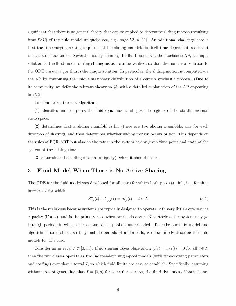
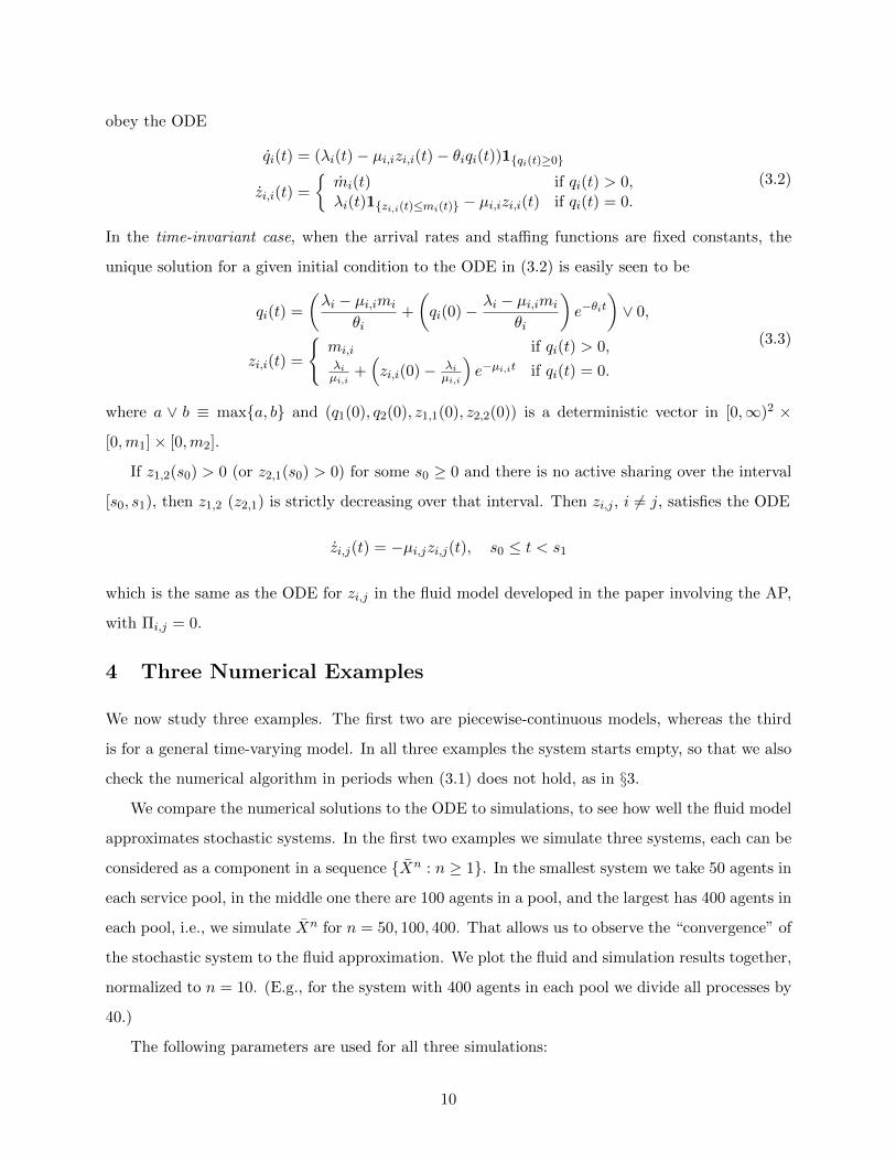
4.1 A Single Overload Incident
The first example aims to check whether FQR-ART detects overloads automatically when they
occur and starts sharing in the right direction, and whether, once an overload incident is over,
FQR-ART avoids oscillations. In particular, over the time interval [0, 60] the arrival rates are as
follows: λn2 = n throughout that time interval. Over [0, 20) and [40, 60] the arrival rate to pool 1 is
λn1 = n. Hence, both pools are normally loaded during these two subintervals. However, during the
interval [20, 40) the arrival rate of class 1 changes to λn1 = 1.4n, so that, during [20, 40) the system
is overloaded, and pool 2 should be helping class 1.
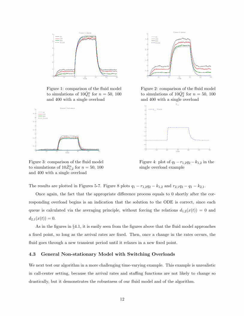
We compare the solution to the fluid equations, solved using the algorithm, to an average of
1000 independent simulation runs for the three cases n = 50, 100, 400. The results are shown in
Figures 1-3 below. In addition Figure 4 plots q1 − r1,2q2 − k1,2. Since shortly after time 20 the
value is 0 in Figure 4, we have a strong indication that the numerical solution is correct, because
during most of the overload period, when sharing takes place, it should hold that d1,2(x(t)) = 0.
The simulation experiments indicate that the fluid model approximates well the mean behavior
of the system even for relatively small systems, e.g., when n = 50. Of course, the accuracy of
the approximation grows as n becomes larger. The simulation experiments show that FQR-ART
quickly detects the overload and the correct direction of sharing. Moreover, the control ensures
that there are no oscillations.
Another observation is that when the system is normally loaded and there is no sharing, the
fluid model, which has null queues, does not describe the queues well. In those cases there is an
increased importance to stochastic refinements for the queues. If there is only negligible sharing,
as FQR-ART ensures, then such stochastic refinements are well approximated by diffusion limits
for the Erlang A model, as in Garnett et al. (2002).
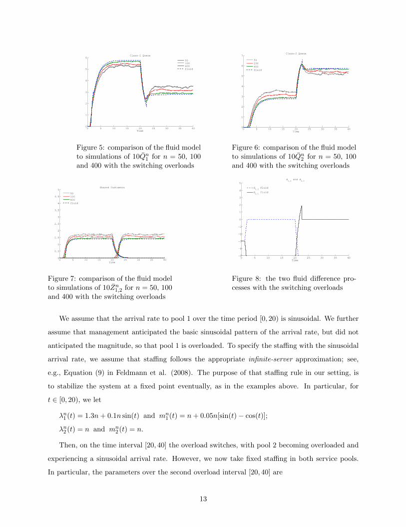
4.2 Switching Overloads
In the second example we consider an overloaded system, with pool 1 being overloaded initially, and
with the direction of overload switching after some time, making pool 2 overloaded. Specifically,
we let the arrival rates be λn1 = 1.4n and λn2 = n over [0, 20), and λn1 = n, λn2 = 1.4n on [20, 40].
11
0 10 20 30 40 50 600
1
2
3
4
5
6Class−1 Queue
Time
50100400fluid
Figure 1: comparison of the fluid modelto simulations of 10Qn1 for n = 50, 100and 400 with a single overload
0 10 20 30 40 50 600
0.5
1
1.5
2
2.5
3
3.5
4Class−2 Queue
Time
50100400fluid
Figure 2: comparison of the fluid modelto simulations of 10Qn2 for n = 50, 100and 400 with a single overload
0 10 20 30 40 50 600
0.5
1
1.5
2
2.5
3
3.5
4
4.5
5Shared Customers
Time
50100400fluid
Figure 3: comparison of the fluid modelto simulations of 10Zn1,2 for n = 50, 100and 400 with a single overload
0 10 20 30 40 50 60−5
−4
−3
−2
−1
0
1
2
3
4
5d
1,2
Time
d1,2
fluid
Figure 4: plot of q1− r1,2q2−k1,2 in thesingle overload example
The results are plotted in Figures 5-7. Figure 8 plots q1 − r1,2q2 − k1,2 and r2,1q2 − q1 − k2,1.
Once again, the fact that the appropriate difference process equals to 0 shortly after the cor-
responding overload begins is an indication that the solution to the ODE is correct, since each
queue is calculated via the averaging principle, without forcing the relations d1,2(x(t)) = 0 and
d2,1(x(t)) = 0.
As in the figures in §4.1, it is easily seen from the figures above that the fluid model approaches
a fixed point, so long as the arrival rates are fixed. Then, once a change in the rates occurs, the
fluid goes through a new transient period until it relaxes in a new fixed point.
4.3 General Non-stationary Model with Switching Overloads
We next test our algorithm in a more challenging time-varying example. This example is unrealistic
in call-center setting, because the arrival rates and staffing functions are not likely to change so
drastically, but it demonstrates the robustness of our fluid model and of the algorithm.
12
0 5 10 15 20 25 30 35 400
1
2
3
4
5
6Class−1 Queue
Time
50100400fluid
Figure 5: comparison of the fluid modelto simulations of 10Qn1 for n = 50, 100and 400 with the switching overloads
0 5 10 15 20 25 30 35 400
1
2
3
4
5
6
7Class−2 Queue
Time
50100400fluid
Figure 6: comparison of the fluid modelto simulations of 10Qn2 for n = 50, 100and 400 with the switching overloads
0 5 10 15 20 25 30 35 400
0.5
1
1.5
2
2.5
3
3.5
4
4.5
5Shared Customers
Time
50100400fluid
Figure 7: comparison of the fluid modelto simulations of 10Zn1,2 for n = 50, 100and 400 with the switching overloads
0 5 10 15 20 25 30 35 40−5
−4
−3
−2
−1
0
1
2
3
4
5
d1,2
and d2,1
Time
d1,2
fluid
d2,1
fluid
Figure 8: the two fluid difference pro-cesses with the switching overloads
We assume that the arrival rate to pool 1 over the time period [0, 20) is sinusoidal. We further
assume that management anticipated the basic sinusoidal pattern of the arrival rate, but did not
anticipated the magnitude, so that pool 1 is overloaded. To specify the staffing with the sinusoidal
arrival rate, we assume that staffing follows the appropriate infinite-server approximation; see,
e.g., Equation (9) in Feldmann et al. (2008). The purpose of that staffing rule in our setting, is
to stabilize the system at a fixed point eventually, as in the examples above. In particular, for
t ∈ [0, 20), we let
λn1 (t) = 1.3n+ 0.1n sin(t) and mn1 (t) = n+ 0.05n[sin(t)− cos(t)];
λn2 (t) = n and mn2 (t) = n.
Then, on the time interval [20, 40] the overload switches, with pool 2 becoming overloaded and
experiencing a sinusoidal arrival rate. However, we now take fixed staffing in both service pools.
In particular, the parameters over the second overload interval [20, 40] are
13

λn1 (t) = n and mn1 (t) = n; λn2 (t) = 1.1n+ 0.1n sin(t) and mn
2 (t) = n.
Thus, we test two overload settings in this example. In the first interval, we can see whether the
fluid approximation stabilizes. Since there is sharing of class-1 customers, previous results such as
in Liu and Whitt (2012a) do not apply directly to our case. In the second interval, we expect to
see a sinusoidal behavior of the system, because the staffing in both pools is fixed. In particular,
the fluid model should not approach a fixed point after the switch at time t = 20.
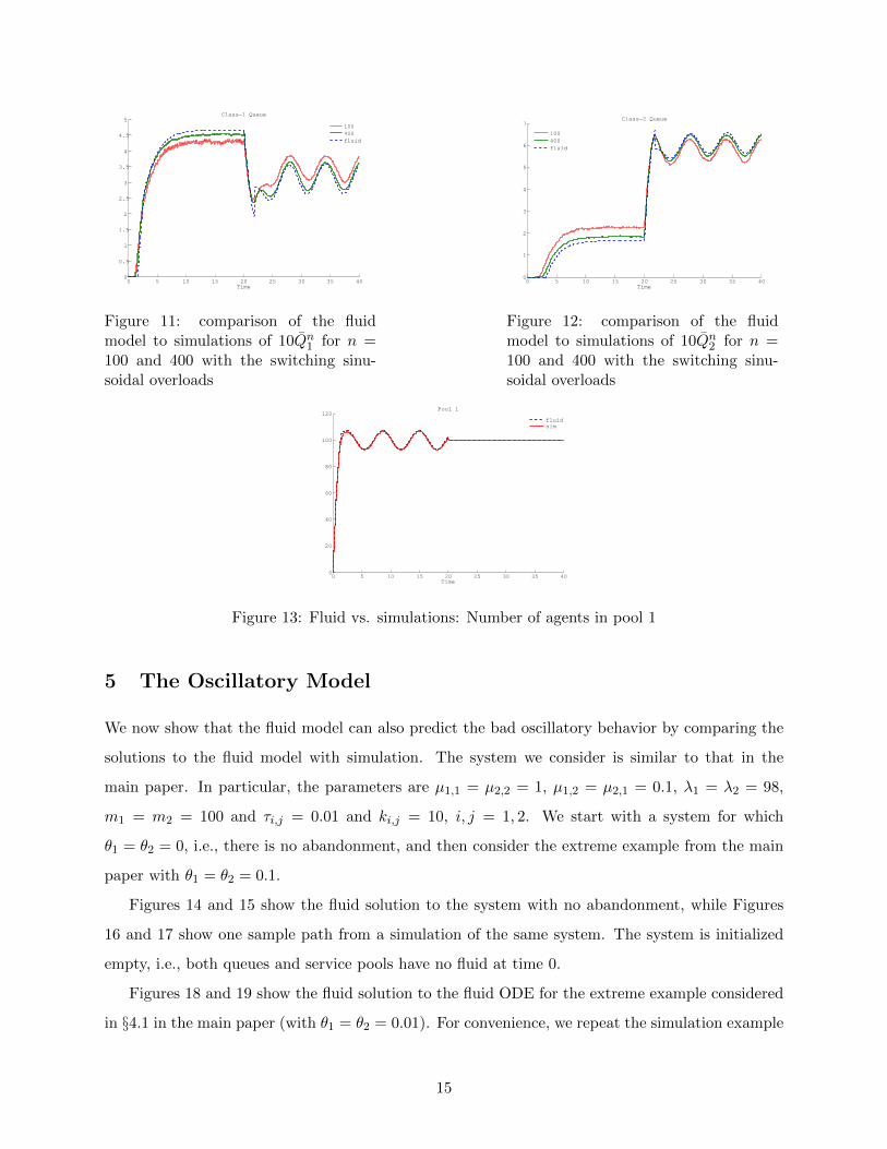
We compare the fluid approximation to simulations for n = 100 and n = 400. Figures 9–12
demonstrate the effectiveness of the fluid model and the numerical algorithm. As expected, the
fluid over [0, 20) approaches a fixed point, and exhibits a sinusoidal behavior after t = 20, with the
accuracy of the fluid approximation increasing in the scale parameter n.
0 5 10 15 20 25 30 35 40−5
−4
−3
−2
−1
0
1
2
3
4
5
d1,2
and d2,1
Time
d1,2
fluid
d2,1
fluid
Figure 9: the two fluid difference func-tions d1,2 and d2,1 with the switchingsinusoidal overloads
0 5 10 15 20 25 30 35 400
0.5
1
1.5
2
2.5
3
3.5
4
4.5
5Shared Customers
Time
100400fluid
Figure 10: comparison of the fluidmodel to simulations of 10Zn1,2 and10Zn2,1 for n = 100 and 400 with theswitching sinusoidal overloads
As was mentioned above, the fluid model requires special care when the staffing functions are
decreasing; see Liu and Whitt (2012a). Figure 13 shows the actual number of agents in Pool 1
for the case n = 100 (the average of the 1000 simulations), and the staffing function mn1 (t) given
above. Clearly, the fluid model follows the actual staffing closely. We further note that there is a
downward jump in the staffing function at time t = 20. In the fluid model, we simply eliminated the
appropriate amount of staffing from the pool, together with the fluid that was processed with that
removed capacity (this fluid in service is lost). However, in the simulation, agents are removed only
when they are done serving, so there is no jump in the actual staffing at t = 20, and no customer
in service is lost. Nevertheless, the fluid model with the jump is clearly a good approximation for
the stochastic model with no jump. This behavior is to be expected, since there are many service
completions over short time intervals in large systems.
14
0 5 10 15 20 25 30 35 400
0.5
1
1.5
2
2.5
3
3.5
4
4.5
5Class−1 Queue
Time
100400fluid
Figure 11: comparison of the fluidmodel to simulations of 10Qn1 for n =100 and 400 with the switching sinu-soidal overloads
0 5 10 15 20 25 30 35 400
1
2
3
4
5
6
7Class−2 Queue
Time
100400fluid
Figure 12: comparison of the fluidmodel to simulations of 10Qn2 for n =100 and 400 with the switching sinu-soidal overloads
0 5 10 15 20 25 30 35 400
20
40
60
80
100
120Pool 1
Time
fluidsim
Figure 13: Fluid vs. simulations: Number of agents in pool 1
5 The Oscillatory Model
We now show that the fluid model can also predict the bad oscillatory behavior by comparing the
solutions to the fluid model with simulation. The system we consider is similar to that in the
main paper. In particular, the parameters are µ1,1 = µ2,2 = 1, µ1,2 = µ2,1 = 0.1, λ1 = λ2 = 98,
m1 = m2 = 100 and τi,j = 0.01 and ki,j = 10, i, j = 1, 2. We start with a system for which
θ1 = θ2 = 0, i.e., there is no abandonment, and then consider the extreme example from the main
paper with θ1 = θ2 = 0.1.
Figures 14 and 15 show the fluid solution to the system with no abandonment, while Figures
16 and 17 show one sample path from a simulation of the same system. The system is initialized
empty, i.e., both queues and service pools have no fluid at time 0.
Figures 18 and 19 show the fluid solution to the fluid ODE for the extreme example considered
in §4.1 in the main paper (with θ1 = θ2 = 0.01). For convenience, we repeat the simulation example
15

0 100 200 300 400 5000
10
20
30
40
50
60
70
80
90
100
z1,2
Figure 14: Oscillations z1,2(t) in thefluid model of the extreme example withno abandonment.
0 100 200 300 400 5000
1000
2000
3000
4000
5000
6000
Time
q2
Figure 15: Oscillating growth of thecontent q2(t) in the fluid model of theextreme example with no abandonment.
0 100 200 300 400 500 600 700 8000
0.1
0.2
0.3
0.4
0.5
0.6
0.7
0.8
0.9
1Proportion of type 2 servers serving class 1 customers
Time
Proportion
Figure 16: Oscillations of Zn1,2 in theextreme symmetric example with τni,j =1, kni,j = 10 and no abandonment.
0 100 200 300 400 500 600 700 8000
1000
2000
3000
4000
5000
6000
7000
8000
9000Number of customers in class 2 queue
Time
Number in queue
Figure 17: Oscillating growth of Qn2 inthe extreme symmetric example withτni,j = 1, kni,j = 10 and no abandonment.
in Figures 20 and 21. Note that the initial conditions here are different than in Figures 16–21. We
now take z1,1(0) = m1 = 100 and z1,2(0) = m2 − z2,2(0) = 20. The reason is that, if the fluid
is initialized with no sharing and no queues, then its components (q1, q2, z1,2, z2,1) are fixed at
(0, 0, 0, 0), i.e., there is never any sharing, and the fluid queues are constant at zero. However, if
it is initialized at states with some sharing, then it may get stuck at an oscillatory equilibrium, as
shown in Figures 14 – 19. In particular, this is a numerical example that the fluid model may be
bi-stable, namely, have two very different stationary behaviors. To which stationary behavior the
fluid ends up converging depends on the initial condition.
This fluid bi-stability property has two immediate implications to the stochastic system. First,
once an overload incident is ending, with substantial sharing taking place, the system may start to
oscillate. The second implication is that the no-sharing equilibrium may be unstable in practice,
because stochastic noise can eventually “push” the system out of this equilibrium, and cause it to
16

0 500 1000 15000
10
20
30
40
50
60
70
80
90
100
z1,2
Figure 18: Oscillations z1,2(t) in thefluid model of the extreme example withabandonment.
0 500 1000 15000
500
1000
1500
q2
Figure 19: Oscillating growth of thecontent q2(t) in the fluid model of theextreme example with abandonment.
0 500 1000 15000
0.1
0.2
0.3
0.4
0.5
0.6
0.7
0.8
0.9
1Proportion of type 2 servers serving class 1 customers
Time
Proportion
Figure 20: Oscillations of Zn1,2 in the extremesymmetric example with τni,j = 1, kni,j = 10with abandonment.
0 500 1000 15000
200
400
600
800
1000
1200
1400
1600
1800Number of customers in class 2 queue
Time
Figure 21: Oscillating stable behavior ofQn2 in the extreme symmetric example withτni,j = 1, kni,j = 10 with abandonment.
oscillate, as demonstrated in Figures 16 and 17. (Recall that the initial condition in this example
was an empty system. In particular, with no sharing initially.) Note also that the time scale in
Figures 14 and 15 is shorter than in Figures 18 and 19. The time scale of the second example is
longer to make it clear that the system with abandonment converges to an oscillatory equilibrium.
A rigorous treatment of the oscillating fluid model and it consequences to the stochastic system
is taken in Perry and Whitt (2014).
6 QBD Representation for the FTSP
As explained in §6.2 in [26], the FTSP Di,j(γ, ·) can be represented as a QBD for each γ ∈ Bi,j , by
ordering the states such that transitions of the FTSP above and below state 0 are gathered within
blocks. First, we assume that ri,j = j/k, j, k ∈ {1, 2, . . . }, i.e., that ri,j is a rational number, which
is clearly not a limitation from the applied or the computational points of view.
17
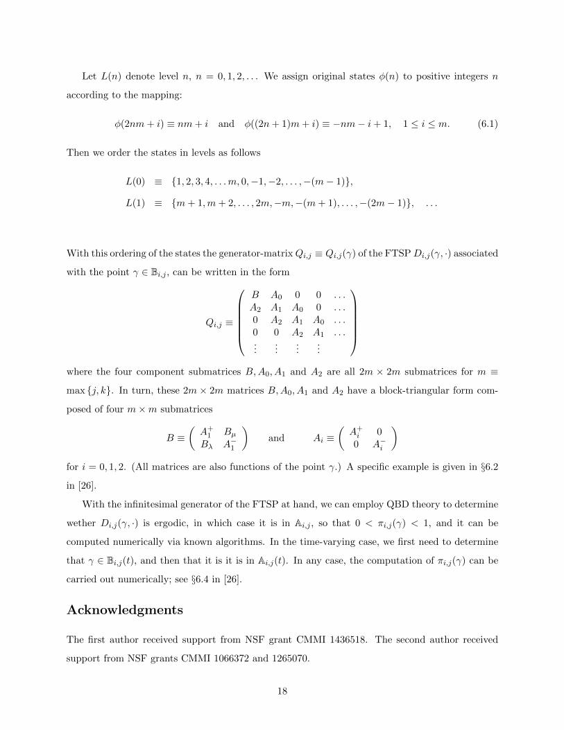
Let L(n) denote level n, n = 0, 1, 2, . . . We assign original states φ(n) to positive integers n
according to the mapping:
φ(2nm+ i) ≡ nm+ i and φ((2n+ 1)m+ i) ≡ −nm− i+ 1, 1 ≤ i ≤ m. (6.1)
Then we order the states in levels as follows
L(0) ≡ {1, 2, 3, 4, . . .m, 0,−1,−2, . . . ,−(m− 1)},
L(1) ≡ {m+ 1,m+ 2, . . . , 2m,−m,−(m+ 1), . . . ,−(2m− 1)}, . . .
With this ordering of the states the generator-matrixQi,j ≡ Qi,j(γ) of the FTSPDi,j(γ, ·) associated
with the point γ ∈ Bi,j , can be written in the form
Qi,j ≡
B A0 0 0 . . .A2 A1 A0 0 . . .0 A2 A1 A0 . . .0 0 A2 A1 . . ....
......
...
where the four component submatrices B,A0, A1 and A2 are all 2m × 2m submatrices for m ≡
max {j, k}. In turn, these 2m × 2m matrices B,A0, A1 and A2 have a block-triangular form com-
posed of four m×m submatrices
B ≡(A+
1 BµBλ A−1
)and Ai ≡
(A+i 0
0 A−i
)for i = 0, 1, 2. (All matrices are also functions of the point γ.) A specific example is given in §6.2
in [26].
With the infinitesimal generator of the FTSP at hand, we can employ QBD theory to determine
wether Di,j(γ, ·) is ergodic, in which case it is in Ai,j , so that 0 < πi,j(γ) < 1, and it can be
computed numerically via known algorithms. In the time-varying case, we first need to determine
that γ ∈ Bi,j(t), and then that it is it is in Ai,j(t). In any case, the computation of πi,j(γ) can be
carried out numerically; see §6.4 in [26].
Acknowledgments
The first author received support from NSF grant CMMI 1436518. The second author received
support from NSF grants CMMI 1066372 and 1265070.
18
References
[1] Aksin, Z., M. Armony, V. Mehrotra. 2007. The modern call center: a multi-disciplinary per-spective on operations management research. Production Oper. Management, 16 (6) 655–688.
[2] Armony, M., S. Israelit, A. Mandelbaum, Y. Marmor, Y. Tseytlin, G. Yom-tov. 2010. Pa-tient flow in hospitals: a data-based queueing-science perspective. Working paper, New YorkUniversity.
[3] Baier, V., R. Fodisch, A. Ihring, E. Kessler, J. Lerchner, G. Wolf, J. M. Kohler, M. Nietzch,M. Krugel. 2006. Highly sensitive thermopile heat power sensor for micro-fluid calorimetry ofbiochemical processes. Sensors and Actuators A 123-124 (23) 354–359.
[4] Berger, A, W., W. Whitt. 1998. Effective bandwidths with priorities. IEEE/ACM Transactionson Networking, 6 (4), 447–460.
[5] Boyle, A., K. Beniuk, I. Higginson, P. Atkinson. 2012. Emergency department crowding: Timefor interventions and policy evaluations. Emergency Medicine J. 29 460–466.
[6] Choudhury G. L., K. K. Leung, W. Whitt. 1995. Efficiently providing multiple grades of servicewith protection against overloads in shared resources. AT&T Technical Journal, 74 (4), 50–63.
[7] Deo, S., I. Gurvich. 2011. Centralized versus decentralized ambulance diversion: a networkperspective. Mangement Sci. 57 (7), 1300–1319.
[8] Doshi, B., H. Heffes. 1986. Overload performance of several processor queueing disciplines forthe M/M/1 queue. IEEE Transactions on Communications, 34 (6), 538–546.
[9] Erramilli, A., L. J. Forys. 1991. Oscillations and chaos in a flow model of a switching system.IEEE journal on Selected Areas in Communications, 9 (2), 171–178.
[10] Feinberg, E. A., M. I. Reiman. 1994. Optimality of randomized trunk reservation. Prob Eng.Inf. Sci. 8 (4) 463–489.
[11] Filippov, A. F. (1988) Differential Equations with Discontinuous Righthand Sides. KluwerAcademic Publishers, the Netherlands.
[12] Floyd, S., K. Fall. 1999. Promoting the use of end-to-end congestion control in the InternetIEEE/ACM Transactions on Networking, 7 (4), 458–472.
[13] Goldstein, M. A., K. A. Kavajecz. 2004. Trading strategies during circuit breakers and extrememarket movements. Journal of Financial Markets, 7 301–333.
[14] Gurvich, I., W. Whitt. 2009a. Queue-and-idleness-ratio controls in many-server service sys-tems. Math. Oper. Res. 34 (2) 363–396.
[15] Gurvich, I., W. Whitt. 2009b. Scheduling flexible servers with convex delay costs in many-server service systems. Manufacturing Service Oper. Management 11 (2) 237–253.
[16] Gurvich, I., W. Whitt. 2010. Service-level differentiation in many-server service systems viaqueue-ratio routing. Oper. Res. 58 (2) 316–328.
[17] Kelly, F. P. 1991. Loss networks. Ann. Appl. Probab. 1 (3), 319–378.
19

[18] Khalil, H. K. 2002. Nonlinear Systems. Prentice Hall, New Jersey.
[19] Korner U. 1991. Overload control of SPC systems. International Teletraffic Congress, ITC 13,Copenhagen, Denmark.
[20] Liberzon, D. (2003) Switching in Systems and Control. Birkhauser, Boston.
[21] Liu, Y., W. Whitt. 2011. Nearly periodic behavior in the the overloaded G/D/S+GI Queue.Stochastic Systems 1 (2) 340–410.
[22] Low, S. H., F. Paganini, J. C. Doyle. 2002. Internet congestion control. Control Systems, 22(1), 28–43.
[23] Matveev, A. S., Savkin, A. V. (2000). Qualitative theory of hybrid dynamical systems.Birkhauser, Boston.
[24] Perry, O., W. Whitt. 2009. Responding to unexpected overloads in large-scale service systems.Management Sci., 55 (8), 1353–1367.
[25] Perry, O., W. Whitt. 2011a. A fluid approximation for service systems responding to unex-pected overloads. Oper. Res., 59 (5), 1159–1170.
[26] Perry, O., W. Whitt. 2011b. An ODE for an overloaded X model involving a stochastic aver-aging principle. Stochastic Systems, 1 (1), 17–66.
[27] Perry, O., W. Whitt. 2013a. A fluid limit for an overloaded X model via a stochastic averagingprinciple. Math, Oper. Res. 13 (2), 294–349.
[28] Perry, O., W. Whitt. 2014. Diffusion approximation for an overloaded X model via a stochasticaveraging principle. Queueing Systems 76, 347–401.
[29] Perry, O., W. Whitt. 2014. A switching fluid limit of a stochastic network under astate-space-collapse inducing control with chattering. Working paper. Available online:http://www.columbia.edu/∼ww2040/recent.html
[30] Schaft, V.D. and Schumacher, H. (2000). An introduction to hybrid dynamical systems SpringerLecture Notes in Control and Information Sciences, Vol. 251. Springer-Verlag, London.
[31] Schulzrinne, H., J. F. Kurose, D. Towsley. 1990. Congestion control for real-time traffic in high-speed networks. IEEE proceeding in Ninth Annual Joint Conference of the IEEE Computerand Communication Societies, 543–550.
[32] Shah, D., D. Wischik. 2011. Fluid models of congestion collapse in overloaded switched net-works. Queueing Systems 69 121–143.
[33] Sontag, E. D. 1998. Mathematical Control Theory, second edition, Springer, New York.
[34] Weber, J. H. 1964. A simulation study of routing control in communication networks. BellSystem Tech. J. 43 2639–2676.
[35] Wei, D. X., C. Jin, S. H. Low, S. Hegde. 2006. FAST TCP: motivation, architecture, algorithms,performance. IEEE/ACM Transactions on Networking, 14 (6), 1246–1259.
[36] Wilkinson, R. I. 1956. Theory for toll traffic engineering in the U.S.A. Bell System Tech. J.35 421–513.
20

[37] Yankovic, N., S. Glied, L. V. Green, M. Grams. 2010. The impact of ambulance diversion onheart attack deaths. Inquiry 47 (1) 81–91.
21