online stress corrosion crack and fatigue usages factor monitoring … · 2015-01-15 ·...
TRANSCRIPT

ANL/LWRS-14/02
Online Stress Corrosion Crack and Fatigue Usages
Factor Monitoring and Prognostics in Light Water
Reactor Components: Probabilistic Modeling, System
Identification and Data Fusion Based Big Data
Analytics Approach
Nuclear Engineering Division

About Argonne National Laboratory Argonne is a U.S. Department of Energy laboratory managed by UChicago Argonne, LLC under contract DE-AC02-06CH11357. The Laboratory’s main facility is outside Chicago, at 9700 South Cass Avenue, Argonne, Illinois 60439. For information about Argonne and its pioneering science and technology programs, see www.anl.gov.
DOCUMENT AVAILABILITY
Online Access: U.S. Department of Energy (DOE) reports produced after 1991 and a growing number of pre-1991 documents are available free via DOE's SciTech Connect (http://www.osti.gov/scitech/) Reports not in digital format may be purchased by the public from the National Technical Information Service (NTIS):
U.S. Department of Commerce National Technical Information Service 5301 Shawnee Rd Alexandra, VA 22312 www.ntis.gov Phone: (800) 553-NTIS (6847) or (703) 605-6000 Fax: (703) 605-6900 Email: [email protected]
Reports not in digital format are available to DOE and DOE contractors from the Office of Scientific and Technical Information (OSTI):
U.S. Department of Energy Office of Scientific and Technical Information P.O. Box 62 Oak Ridge, TN 37831-0062 www.osti.gov Phone: (865) 576-8401 Fax: (865) 576-5728 Email: [email protected]
Disclaimer
This report was prepared as an account of work sponsored by an agency of the United States Government. Neither the United States
Government nor any agency thereof, nor UChicago Argonne, LLC, nor any of their employees or officers, makes any warranty, express
or implied, or assumes any legal liability or responsibility for the accuracy, completeness, or usefulness of any information, apparatus,
product, or process disclosed, or represents that its use would not infringe privately owned rights. Reference herein to any specific
commercial product, process, or service by trade name, trademark, manufacturer, or otherwise, does not necessarily constitute or imply
its endorsement, recommendation, or favoring by the United States Government or any agency thereof. The views and opinions of
document authors expressed herein do not necessarily state or reflect those of the United States Government or any agency thereof,
Argonne National Laboratory, or UChicago Argonne, LLC.

ANL/LWRS-14/02
Online Stress Corrosion Crack and Fatigue Usages Factor Monitoring and Prognostics in Light Water Reactor Components: Probabilistic Modeling, System Identification and Data Fusion Based Big Data Analytics Approach
Subhasish Mohanty1, Bryan Jagielo2, William Iverson3, Chi Bum Bhan4, William
Soppet1, Saurin Majumdar1, and Ken Natesan1
1Nuclear Engineering Division, Argonne National Laboratory
22014 DOE-SULI summer intern at Argonne National Laboratory from Oakland
University, Rochester
32014 DOE-SULI summer intern at Argonne National Laboratory from University of
Illinois, at Urbana-Champaign, Champaign
4Former Employee of Argonne National Laboratory, Currently at Pusan National
University, South Korea
September 2014

Online Stress Corrosion Crack and Fatigue Usages Factor Monitoring and Prognostics in Light Water Reactor Components: Probabilistic Modeling, System Identification and Data Fusion Based Big Data Analytics Approach September 2014

This page intentionally left blank


Online Stress Corrosion Crack and Fatigue Usages Factor Monitoring and Prognostics in Light Water Reactor Components: Probabilistic Modeling, System Identification and Data Fusion Based Big Data Analytics Approach September 2014
ANL/LWRS-14/02
i
ABSTRACT
Nuclear reactors in the United States account for roughly 20% of the nation's total electric energy
generation, and maintaining their safety in regards to key component structural integrity is
critical not only for long term use of such plants but also for the safety of personnel and the
public living around the plant. Early detection of damage signature such as of stress corrosion
cracking, thermal-mechanical loading related material degradation in safety-critical components
is a necessary requirement for long-term and safe operation of nuclear power plant systems. At
present, only preventative maintenance and in-service inspection through nondestructive
evaluation (NDE) techniques are viable methods for damage detection and quantification.
However, the current state of the art nondestructive evaluation (NDE) techniques used in nuclear
reactor structural inspection are manual, labor intensive, time consuming, and only used when
the reactor has been shut down. Despite periodic inspection of plant components, a failure mode
such as stress corrosion and/or fatigue crack can initiate in between two scheduled inspections
and can become critical before the next scheduled inspection. In this context, real time
monitoring of nuclear reactor components is necessary for continuous and autonomous health
monitoring and life prognosis of safety critical reactor components. However real time
monitoring of structural components is a highly complex multidisciplinary area requiring
intermixing of knowledge base in advanced structural mechanics (such as in fracture mechanics,
material damage physics modeling) with knowledge base in big data analytics approaches (such
as in data mining probabilistic modeling, system identification, data fusion, etc.).
In this report, first the basic background and futuristic scopes related to online structural health
monitoring and prognostics are discussed. Then the basic concepts behind structural health
monitoring and prognostic are demonstrated through two examples such as through a) the
demonstration of various system identification and data fusion based approaches for online
monitoring of stress corrosion cracking in a pressurized water reactor steam generator tube using
active ultrasonic sensor networks b) then through the demonstration of a framework for real time
estimation of probabilistic fatigue usages factor and remaining life of light water reactor steel
based on real time strain measurements under different environmental and loading conditions.
The report is organized into three major sections such as:
1. A Futuristic Online Structural Health Monitoring and Prognostics Framework for US
Nuclear Reactors.
2. Linear and Nonlinear System Identification and Sensor Data Fusion Based Big Data
Analytics Approach for Stress Corrosion Crack Monitoring in Nuclear Reactor
Components Using Active Ultrasonic Sensor Networks.
3. Gaussian Process Based Probabilistic Framework for Online Fatigue Usage Factor
Monitoring & Remaining Life Forecasting in Nuclear Reactor Components.

Online Stress Corrosion Crack and Fatigue Usages Factor Monitoring and Prognostics in Light Water Reactor Components: Probabilistic Modeling, System Identification and Data Fusion Based Big Data Analytics Approach September 2014
ANL/LWRS-14/02 ii
This page intentionally left blank

Online Stress Corrosion Crack and Fatigue Usages Factor Monitoring and Prognostics in Light Water Reactor Components: Probabilistic Modeling, System Identification and Data Fusion Based Big Data Analytics Approach September 2014
ANL/LWRS-14/02
iii
TABLE OF CONTENTS
ABSTRACT i
Table of Contents iii
List of Figures iv
Abbreviations viii
Acknowledgments ix
1 A Futuristic Online Structural Health Monitoring and Prognostics Framework for US
Nuclear Reactors 10
1.1 Introduction ................................................................................................................... 10
1.2 Online structural health monitoring .............................................................................. 10
1.3 Online Structural Health Prognostics........................................................................... 12
2 Linear and Nonlinear System Identification and Sensor Data Fusion Based Big Data
Analytics Approach for Stress Corrosion Crack Monitoring in Nuclear Reactor
Components Using Active Ultrasonic Sensor Networks 13
2.1 Introduction ................................................................................................................... 13
2.2 Experiments and OSHM System Design ...................................................................... 13
2.2.1 Experimental Setup, Pulse Generation, and Data Acquisition 14
2.2.2 Fast Scale Signal Processing 16
2.2.3 Slow-Scale Damage Anomaly Estimation 20
2.2.4 Multi-Node Sensor Data Fusion 49
2.3 Conclusion .................................................................................................................... 54
3 A Bayesian Statistic Based Probabilistic Framework for Online Fatigue Usage Factor
Monitoring & Remaining Life Forecasting in Nuclear Reactor Components 55
3.1 Introduction ................................................................................................................... 55
3.2 Theoretical Background ................................................................................................ 55
3.2.1 Online mean usage factor and remaining useful life prediction under in-air-
fatigue loading 55
3.2.2 Probabilistic modeling of usage factor and remaining useful life 57
3.2.3 Online mean and probabilistic usage factor and remaining useful life
prediction under light water reactor environment condition fatigue loading 59
3.3 Numerical Results ......................................................................................................... 61
3.3.1 High purity water and elevated temperature live fatigue test 61
3.3.2 PWR water and elevated temperature live fatigue test 71
3.3.3 In-air and room temperature live fatigue test 74
3.3.4 Simulated random strain transients under PWR water condition 78
3.4 Conclusions ................................................................................................................... 82

Online Stress Corrosion Crack and Fatigue Usages Factor Monitoring and Prognostics in Light Water Reactor Components: Probabilistic Modeling, System Identification and Data Fusion Based Big Data Analytics Approach September 2014
ANL/LWRS-14/02 iv
LIST OF FIGURES
Figure 1. 1 A fault tree diagram of a national level OSHM system. ........................................ 11
Figure 1. 2 Schematic of already degraded states of structure estimated through an OSHM
system and forecasted states and their probability bound through an OLP system. .. 12
Figure 2. 1 A schematic of the fast scale pulsing in reference to the slow scale process. ........ 14
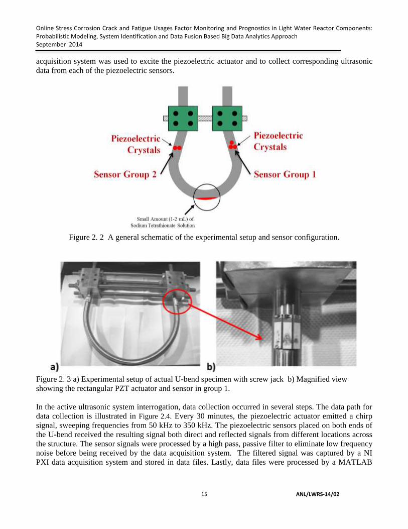
Figure 2. 2 A general schematic of the experimental setup and sensor configuration. ........... 15
Figure 2. 3 a) Experimental setup of actual U-bend specimen with screw jack b) Magnified
view showing the rectangular PZT actuator and sensor in group 1. .......................... 15
Figure 2. 4 Data acquisition and processing path of OSHM system. ...................................... 16
Figure 2. 5 Sample signal from actuator, sensor group 1, sensor group 2, and noise sensor. . 17
Figure 2. 6 Sample spectrogram of signal from actuator, sensor group 1, sensor group 2, and
noise sensor. ............................................................................................................... 18
Figure 2. 7 Selected signal from original sample of signal from actuator, sensor group 1 ..... 19
Figure 2. 8 Example spectrogram of windowed and filtered signal from actuator, sensor
group 1, sensor group 2, and noise sensor. ................................................................ 20
Figure 2. 9 Scatter plot of first, quarter life, half-life, three quarters life, and end of life
complete signal from sensor group 1 and sensor group 2. ........................................ 21
Figure 2. 10 Scatter plot of first, quarter life, half-life, three-quarters life, and end of life
windowed and filtered signal from sensor group 1 and sensor group 2. .................. 22
Figure 2. 11 Calculated means from sensor group 1 and sensor group 2 ............................... 23
Figure 2. 12 Calculated variances from sensor group 1 and sensor group 2. ......................... 24
Figure 2. 13 Covariance between actuator and sensor group 1 and actuator and sensor
group 2. ...................................................................................................................... 25
Figure 2. 14 Covariance between sensor group 1 and sensor group 2. .................................... 26
Figure 2. 15 Sample scatter plot of mapping between sensors in group 1 with regression
line.............................................................................................................................. 27
Figure 2. 16 Linear fit parameters for mapping between actuator and sensor group 1. .......... 28
Figure 2. 17 Linear fit parameters for mapping between actuator and sensor group 2 ........... 29
Figure 2. 18 Linear fit parameters for mapping between sensors in group 1 and sensors in
group 2. ...................................................................................................................... 30
Figure 2. 19 Plot of the damage index computed from linear mapping between sensors in
group 1. ...................................................................................................................... 31
Figure 2. 20 Plot of the damage index computed from linear mapping between sensors in
group 2. ...................................................................................................................... 31
Figure 2. 21 Predicted and actual output using CRA mapping between sensors in group 1. .. 33
Figure 2. 22 Prediction and actual output using CRA mapping between sensors in group 2. . 33
Figure 2. 23 Computed damage index from CRA mapping between sensors in group 1........ 34
Figure 2. 24 Computed damage index from CRA mapping between sensors in group 2........ 35
Figure 2. 25 Predicted and actual output using ETFE mapping between sensors in group 1. . 36

Online Stress Corrosion Crack and Fatigue Usages Factor Monitoring and Prognostics in Light Water Reactor Components: Probabilistic Modeling, System Identification and Data Fusion Based Big Data Analytics Approach September 2014
ANL/LWRS-14/02
v
Figure 2. 26 Predicted and actual output using ETFE mapping between sensors in group 2. . 37
Figure 2. 27 Computed damage index from ETFE mapping between sensors in group 1. ..... 38
Figure 2. 28 Computed damage index from ETFE mapping between sensors in group 2. ..... 38
Figure 2. 29 Predicted output with two standard deviation error bounds and predicted and
actual output from mapping between sensors in group 1. ......................................... 41
Figure 2. 30 Magnified version of Figure 2.29. ........................................................................ 42
Figure 2. 31 Predicted output with two standard deviation error bounds and predicted and
actual output from mapping between sensors in group 2. ......................................... 42
Figure 2. 32 Magnified version of Figure 2.31. ....................................................................... 43
Figure 2. 33 Hyperparameters for Gaussian Process model computed between sensors in
group 1. ...................................................................................................................... 44
Figure 2. 34 Hyperparameters for Gaussian Process model computed between sensors in
group 2. ...................................................................................................................... 44
Figure 2. 35 ℓ2-norm of hyperparameters computed between sensors in group 1. ................. 45
Figure 2. 36 ℓ2-norm of hyperparameters computed between sensors in group 2. ................. 45
Figure 2. 37 Computed prediction error for Gaussian Process mapping between sensors in
group 1. ...................................................................................................................... 46
Figure 2. 38 Computed prediction error for Gaussian Process mapping between sensors in
group 2. ...................................................................................................................... 47
Figure 2. 39 Computed baseline referenced damage index for Gaussian Process mapping
between sensors in group 1. ....................................................................................... 48
Figure 2. 40 Computed baseline referenced damage index for Gaussian Process mapping
between sensors in group 2 ........................................................................................ 48
Figure 2. 41 A diagram of the data path for PCA dimension reduction. ................................. 49
Figure 2. 42 All damage index time series from Gaussian Process mapping. ......................... 51
Figure 2. 43 Computed damage index using Gaussian Process mapping and PCA based
sensor fusion. ............................................................................................................. 51
Figure 2. 44 A picture of the U-bend pipe specimen after test. ............................................... 52
Figure 2. 45 The damage index computed with Gaussian Process and PCA at quarter-life,
half-life, three quarters life, and end of life. .............................................................. 53
Figure 2. 46 The damage index computed recursively at each damage level with the
Gaussian Process and PCA and range in computed damage indices due to
mathematical error. .................................................................................................... 53
Figure 3. 1 ANL environmental test frame with live fatigue monitoring system ..................... 62
Figure 3. 2 Intermittent cyclic stress history for the high purity water fatigue test ................. 65
Figure 3. 3 Magnified stress history ........................................................................................ 66
Figure 3. 4 Intermittent transformed cyclic strain history for the high purity water fatigue
test using stroke-strain mapping ................................................................................ 66
Figure 3. 5 Time history of environmental correction factor 𝐹𝑒𝑛𝑘 ....................................... 67

Online Stress Corrosion Crack and Fatigue Usages Factor Monitoring and Prognostics in Light Water Reactor Components: Probabilistic Modeling, System Identification and Data Fusion Based Big Data Analytics Approach September 2014
ANL/LWRS-14/02 vi
Figure 3. 6 Stroke sensor measurement based real time estimated usages factor time history
for the high purity water fatigue test using both NUREG-6909 based approach and
GP based approach ..................................................................................................... 67
Figure 3. 7 Load cell or stress sensor measurement based real time estimated usages factor
time history for the high purity water fatigue test using both NUREG-6909 based
approach and GP based approach .............................................................................. 68
Figure 3. 8 Strain Amplitude vs Fatigue Life for stainless steel in PWR high temperature
water ........................................................................................................................... 68
Figure 3. 9 Example histogram and probability density function of logarithmically scaled
fatigue life approximately at 0.6 % strain amplitude for PWR data shown in Figure
3.8............................................................................................................................... 69
Figure 3. 10 GP estimated logarithmically scaled mean cycle to failure and associated 2σ
confidence bound as estimated at any given fatigue cycle ........................................ 69
Figure 3. 11 Stroke sensor measurement based real time forecasted fatigue life for the high
purity water fatigue test specimen at any given fatigue cycle ................................... 70
Figure 3. 12 Load cell sensor measurement based real time forecasted fatigue life for the
high purity water fatigue test specimen at any given fatigue cycle ........................... 70
Figure 3. 13 Intermittent transformed cyclic strain history for the LWR water fatigue test
using stroke-strain mapping ....................................................................................... 72
Figure 3. 14 Time history of environmental correction factor 𝐹𝑒𝑛𝑖 ...................................... 72
Figure 3. 15 GP estimated logarithmically scaled mean cycle to failure and associated 2σ
confidence bound as estimated at any given fatigue cycle ........................................ 73
Figure 3. 16 Stroke sensor measurement based real time estimated usage factor time history
for the PWR water fatigue test using both NUREG-6909 based approach and GP
based approach ........................................................................................................... 73
Figure 3. 17 Strain gage sensor measurement based real time forecasted fatigue life for the
PWR water fatigue test specimen at any given fatigue cycle .................................... 74
Figure 3. 18 Cyclic strain history for the in air fatigue test ..................................................... 75
Figure 3. 19 Strain amplitude vs in-air test fatigue life for stainless steel .............................. 76
Figure 3. 20 Example histogram and probability density function of logarithmically scaled
fatigue life approximately at 0.2% strain amplitude for in-air condition data shown
in Figure 3.19 ............................................................................................................. 76
Figure 3. 21 Strain gage sensor measurement based real time forecasted fatigue life for the
in air fatigue test specimen at any given fatigue cycle .............................................. 77
Figure 3. 22 Strain gage measurement based real time estimated usage factor time history
for the in air fatigue test using both NUREG-6909 based approach and GP based
approach ..................................................................................................................... 77
Figure 3. 23 Strain gage sensor measurement based real time forecasted fatigue life for the
in air fatigue test specimen at any given fatigue cycle .............................................. 78
Figure 3. 24 Pseudorandom cyclic strain history ..................................................................... 79
Figure 3. 25 Time history of environmental correction factor 𝐹𝑒𝑛𝑖 ...................................... 80

Online Stress Corrosion Crack and Fatigue Usages Factor Monitoring and Prognostics in Light Water Reactor Components: Probabilistic Modeling, System Identification and Data Fusion Based Big Data Analytics Approach September 2014
ANL/LWRS-14/02
vii
Figure 3. 26 Predicted logarithmically transformed time history of fatigue life (mean, upper
and lower bounds), as it would be estimated through GP in a realistic reactor
condition .................................................................................................................... 80
Figure 3. 27 Estimated usage factor time history for pseudorandom cycles using both
NUREG-6909 based approach and GP based approach ............................................ 81
Figure 3. 28 Forecasted time history of fatigue life for random cycles ................................... 81
Figure 3. 29 Magnified Figure 3.28 showing clear decreasing trend of cycles to failure ...... 82

Online Stress Corrosion Crack and Fatigue Usages Factor Monitoring and Prognostics in Light Water Reactor Components: Probabilistic Modeling, System Identification and Data Fusion Based Big Data Analytics Approach September 2014
ANL/LWRS-14/02 viii
ABBREVIATIONS
ANL Argonne National Laboratory
CF Corrosion Fatigue
DOE Department of Energy
FEM Finite Element Method
LWR Light Water Reactor
LWRS Light Water Reactor Sustainability
RT Room Temperature
ET Elevated Temperature
SCC Stress Corrosion Cracking
SS Stainless Steel

Online Stress Corrosion Crack and Fatigue Usages Factor Monitoring and Prognostics in Light Water Reactor Components: Probabilistic Modeling, System Identification and Data Fusion Based Big Data Analytics Approach September 2014
ANL/LWRS-14/02
ix
ACKNOWLEDGMENTS
This research was partially supported through the U.S. Department of Energy - Light Water
Reactor Sustainability program under the work package of environmental fatigue study and
partially supported through U.S Nuclear Regulatory Commission sponsored steam generator tube
integrity program. In addition, substantial part of the research was also conducted through two
DOE SULI summer (2014) interns at ANL.

Online Stress Corrosion Crack and Fatigue Usages Factor Monitoring and Prognostics in Light Water Reactor Components: Probabilistic Modeling, System Identification and Data Fusion Based Big Data Analytics Approach September 2014
ANL/LWRS-14/02 10
1 A Futuristic Online Structural Health Monitoring and Prognostics Framework for US Nuclear Reactors
1.1 Introduction
The longevity of safety critical components in the current line of operating nuclear reactors requires the
implementation of regular in-service inspection (ISI) and repair strategies. The current approach for ISI
is to perform nondestructive evaluation (NDE) on the components during routine refueling or
unscheduled shutdowns of the plant. NDE must be performed manually or in a semi-automated way and
in a regular interval. As a result, NDE is costly, time consuming, and puts personnel at risk for exposure
to high doses of radiation. The goal of NDE is to inspect all components to ensure safe operation during
the length of the next usage cycle. However, usage cycle may have a duration at which the previous
NDE is an inappropriate benchmark for the current health of the structure and failures may occur
between inspections. Consequently, on-line structural health monitoring (OSHM) and on-line
prognostics (OLP) are necessary to ensure that the components remain safe for operation during the
entirety of the usage cycle [1-5]. Below, a futuristic OSHM and OLP framework is discussed briefly.
1.2 Online structural health monitoring
Unlike NDE’s periodic manual and/or semi-automated interrogation of structural integrity, OSHM
automatically and continuously interrogates structural health using an array of sensors permanently
bonded to components. These sensors collect information about how components respond to the chosen
interrogation method. The information can be processed and used to determine characteristics about the
system. Under the basis of big data analytics approaches such as system identification, advanced signal
processing, and data mining, the signals recorded by the sensors can be used to determine the changing
transfer function of components. This transfer function can be monitored over time to determine the
deviation of the components from the baseline measurements due to damage growth. The information
can be used for early detection of cracks and relayed to an online prognostics algorithm for further
analysis such as for predicting the remaining life of component based on condition estimated through
OSHM system at any given instant of time.
OSHM system can be scaled up from monitoring of small regions of a component to a national level
monitoring center for monitoring all the structural components of the plants from a centralized location
(say for example from US Nuclear Regulatory Commission head quarter at Washington DC) . Figure 1.1
depicts the schematic of a scaled up system. Each plant can be divided into subsystems containing
components with individual sensor nodes. The sensor nodes can connect to a subsystem network via
wired or wireless connection [1-5]. The subsystem network will relay all of the information from all the
nodes to the plant control center. Plant managers can be presented with real-time continuous updates
regarding the overall plant structural integrity (SI) and can easily diagnose problems quickly down to the
smallest component. Additionally, the health information for each plant can be transmitted to a regional
control center and national control center for further monitoring and regulation. The national monitoring
system would allow in depth aging and health analysis of the nation’s fleet of nuclear plants efficiently
and in real time. This research focuses on a component level real time monitoring framework.

Online Stress Corrosion Crack and Fatigue Usages Factor Monitoring and Prognostics in Light Water Reactor Components: Probabilistic Modeling, System Identification and Data Fusion Based Big Data Analytics Approach September 2014
ANL/LWRS-14/02
11
Scaling up the OSHM system is beyond the scope of this investigation but can be a goal of future work.
up the OSHM system is beyond the scope of this investigation but can be a goal of future work.
Figure 1. 1 A fault tree diagram of a national level OSHM system.

Online Stress Corrosion Crack and Fatigue Usages Factor Monitoring and Prognostics in Light Water Reactor Components: Probabilistic Modeling, System Identification and Data Fusion Based Big Data Analytics Approach September 2014
ANL/LWRS-14/02 12
1.3 Online Structural Health Prognostics
In addition to online monitoring, online prognostics (OLP) can be used to help forecasting the remaining
life of structural components. Currently, no such system available rather the retirement of the
components are decided based on the offline NDE inspection data and/or based on the offline
stress/strain versus life curves. However, there are many restrictions on the accuracy of the current
approach since the stress/strain versus life curves might not always reflect the actual material
microstructure, environment and loading condition the component in question subjected to. In contrary
an OLP system associated with an OSHM system can incorporate real time material condition (e.g.
through material dependent stress-strain hardening/softening), environment (e.g. light water reactor
water chemistry, temperature, etc.) and loading condition (e.g. strain/load amplitude and rate, loading
sequence, etc.). This will not only help to forecast the structural state and remaining useful life (RUL) in
real time, but also will help to provide more accurate results. Figure 1.2 depicts the schematic showing
the forecasted structural states with respect to the OSHM system estimated state information at any
given instant of time.
Figure 1. 2 Schematic of already degraded states of structure estimated through an OSHM system and
forecasted states and their probability bound through an OLP system [1, 4].
In this report, first an ultrasound based approach is discussed, that can be used for online monitoring of
stress corrosion cracking, and then a strain measurement based online fatigue usages factor monitoring
and online remaining life forecasting approaches are discussed, through multiple example cases.

Online Stress Corrosion Crack and Fatigue Usages Factor Monitoring and Prognostics in Light Water Reactor Components: Probabilistic Modeling, System Identification and Data Fusion Based Big Data Analytics Approach September 2014
ANL/LWRS-14/02
13
2 Linear and Nonlinear System Identification and Sensor Data Fusion Based Big Data Analytics Approach for Stress Corrosion Crack Monitoring in Nuclear Reactor Components Using Active Ultrasonic Sensor Networks
(Subhasish Mohanty, Bryan Jagielo, Chi Bum Bhan, Saurin Majumdar, Ken Natesan)
2.1 Introduction
The current state of the art nondestructive evaluation (NDE) techniques used in nuclear reactor structural
inspection are manual labor intensive, time consuming, and only used when the reactor has been shut
down. Also, despite periodic inspection of plant components, a failure mode such as stress corrosion
crack can initiate in between two scheduled inspections and can become critical before the next
scheduled inspection. In this context, real time monitoring of nuclear reactor components is necessary
for continuous and autonomous monitoring of component structural health. In this research, an active
ultrasonic based on-line monitoring (OSHM) framework is developed which can be used for real-time
monitoring of degradation (e.g stress corrosion cracking) of nuclear power plant systems, and
components. Different system identification based methods are investigated to estimate the structural
degradation in real-time. Active broadband ultrasound input is used for damage interrogation and a
multi-sensor data fusion technique is implemented to improve accuracy in state estimation. The damage
index at any particular time is computed using linear techniques such as linear regression, correlation
analysis, and empirical transfer function estimation and nonlinear techniques such as Gaussian Process
probabilistic modeling. The success of each method is discussed and the necessity of sensor fusion is
evaluated. The framework was demonstrated through the monitoring of anomaly trend in a nuclear
reactor steam generator tube undergoing stress corrosion cracking (SCC) testing at ANL’s Steam
Generator Tube Integrity Facilities. The various steps involved are briefly discussed below.
2.2 Experiments and OSHM System Design
The on-line monitoring system estimates the current state of the structure through two components, the
fast scale ultrasonic signal acquisition system and signal processor and the slow scale structural anomaly
(e.g. in this case SCC) state estimator. In the fast scale process the host structure was excited with high
frequency ultrasound waves using a piezoelectric actuator and the respective fast scale sensor signals
were collected and processed. This process was intermittently conducted to capture the entire structural
degradation process. To note that compared to fast scale ultrasound pulsing the structural degradation
process is a slower process and occurs over a very long duration of time. Also note that unlike the low
frequency based vibrations/temperature/strain sensor signals, which are typically, acquired continuously,
the high frequency ultrasound signal cannot be acquired continuously due to large computer memory
and processing time requirements. The intermittently collected fast scale ultrasound signal were
processed first then transferred to a second stage signal processor that estimates the state of the structure
to capture the slow scale damage progression in a structure. To note that in the discussed accelerated
laboratory test case the damage process occurred over multiple hours, however in the real nuclear
reactor components the damage process occurs over years. Hence, two distinct signal processing

Online Stress Corrosion Crack and Fatigue Usages Factor Monitoring and Prognostics in Light Water Reactor Components: Probabilistic Modeling, System Identification and Data Fusion Based Big Data Analytics Approach September 2014
ANL/LWRS-14/02 14
stages/procedures to be followed for ultrasonic based structural damage or anomaly trend estimation.
Figure 2.1 shows a schematic demonstrating the difference between the fast scale ultrasound pulsing and
the slow scale structural anomaly trend. The details of the experiment setup, fast scale signal processing,
and slow scale state estimation are discussed further in the following subsections.
Figure 2. 1 A schematic of the fast scale pulsing in reference to the slow scale process.
2.2.1 Experimental Setup, Pulse Generation, and Data Acquisition
The test setup is a US-NRC sponsored test facility [6] to perform structural integrity test of steam
generator tubes for evaluating SCC under simulated laboratory conditions. While performing usual NRC
regulated tube integrity test, additional instrumentation was made for online monitoring of SCC using
permanently bonded active ultrasonic actuator and sensor nodes. The aim of this exercise was to
demonstrate the basic SHM capability on nuclear reactor component and the overall system can be
scaled up for component, subsystem, plant level, and multi-plant level application as shown in Figure 1.1.
SCC testing was performed on a U-bend pipe specimen. The test setup diagram is illustrated in Figure
2.2 and the actual test setup is displayed in Figure 2.3a. The testing apparatus consisted of a U-bend
section of pipe and a screw jack placed around each end of the specimen. The screw jack was used to
simulate stress on the U-bend by displacing the legs toward the centerline. Sodium Tetrathionate
solution was placed at the apex of the U-bend to accelerate corrosion and cracking within the specimen.
Piezoelectric crystals were permanently bonded to the pipe in two groups near the ends of the U-bend.
Sensor group 1 contained one piezoelectric actuator and two piezoelectric sensors and sensor group 2
contained two piezoelectric sensors. The rectangular type piezoelectric actuator and sensor arrangement
of sensor group 1 is displayed in Figure 2.3b. Additionally, a disk type piezoelectric sensor was placed
in the open air to measure external acoustic and electromagnetic noise. A National Instruments PXI data
Online Stress Corrosion Crack and Fatigue Usages Factor Monitoring and Prognostics in Light Water Reactor Components: Probabilistic Modeling, System Identification and Data Fusion Based Big Data Analytics Approach September 2014
ANL/LWRS-14/02
15
acquisition system was used to excite the piezoelectric actuator and to collect corresponding ultrasonic
data from each of the piezoelectric sensors.
Figure 2. 2 A general schematic of the experimental setup and sensor configuration.
Figure 2. 3 a) Experimental setup of actual U-bend specimen with screw jack b) Magnified view
showing the rectangular PZT actuator and sensor in group 1.
In the active ultrasonic system interrogation, data collection occurred in several steps. The data path for
data collection is illustrated in Figure 2.4. Every 30 minutes, the piezoelectric actuator emitted a chirp
signal, sweeping frequencies from 50 kHz to 350 kHz. The piezoelectric sensors placed on both ends of
the U-bend received the resulting signal both direct and reflected signals from different locations across
the structure. The sensor signals were processed by a high pass, passive filter to eliminate low frequency
noise before being received by the data acquisition system. The filtered signal was captured by a NI
PXI data acquisition system and stored in data files. Lastly, data files were processed by a MATLAB
Online Stress Corrosion Crack and Fatigue Usages Factor Monitoring and Prognostics in Light Water Reactor Components: Probabilistic Modeling, System Identification and Data Fusion Based Big Data Analytics Approach September 2014
ANL/LWRS-14/02 16
signal processing and state estimation algorithm. The design of the MATLAB signal processor and state
estimator will be discussed further in the upcoming sections.
Figure 2. 4 Data acquisition and processing path of OSHM system.
The fast scale signals were collected in real time using National Instruments (NI) based PXI data
acquisition system (as shown in Figure 2.4) and LABVIEW based data acquisition software. Once the
sensor data was acquired at a given instant of time, the slow scale anomaly estimator processed these
signal and estimate the state of the structure at that given instant. A MATLAB based signal processor
and state estimator was developed to work along with LABVIEW for real time monitoring.
2.2.2 Fast Scale Signal Processing
Before the state of the structure can be accurately estimated, the fast scale process signals must be
processed to ensure that they contain the valuable information. The fast scale signal processor designed
incorporates two components: the window selector and frequency filter. The window selector chooses a
portion of the signals containing the least noise for further analysis while attenuates any residual noise
within the windowed signal. The window selector and filter parameters were determined after close
study of the characteristics of the signals. The fast scale process signal is composed of six signals: the
actuator’s input on channel one, the near sensor pair’s output on channels two and three (refer sensor
group 1 Figure 2.2), the far sensor pair’s output on channels four and five (refer sensor group 2), and an
external noise sensor not attached to the structure on channel six. The actuator inputs into the test
structure a broadband chirp signal ranging from 50 kHz to 350 kHz through a PXI pulse generator card.
Simultaneously, all 4 sensor signals (Ch. 2, 3, 4, and 5), noise (Ch. 6), and actuator signal (Ch.1) were
acquired through a PXI ADC input card. Figure 2.5 shows sample signals from each of the channels
during a single chirp pulse on the actuator. The broadband signals have a length of 10ms and were
received at a frequency of 2 MHz, whereas, the broadband input signal was transmitted by the PXI pulse
generator at a frequency of 1 MHz.

Online Stress Corrosion Crack and Fatigue Usages Factor Monitoring and Prognostics in Light Water Reactor Components: Probabilistic Modeling, System Identification and Data Fusion Based Big Data Analytics Approach September 2014
ANL/LWRS-14/02
17
Displayed in Figure 2.5, the signals created by the actuator and observed by the sensors demonstrate
various characteristics. The actuator signals in channel 1 has an initial offset voltage of +3.1V while all
other channels have an offset of 0V. The initial offset voltage in the actuator channel could be due to
residual charge build up due to the capacitive self-sensing nature of the piezoelectric actuator that
receives reflected signals from the structure. The signals were observed to decrease in magnitude as the
distance between the sensor and the actuator increased. The actuator signal, observed in channel 1, had
a peak amplitude of 10V. In contrast, sensor group 1’s signals have a peak amplitude 1.3V in channel 2
and 3.7V in channel 3 while sensor group 2’s signals had a peak amplitude of 0.3V in channel 4 and
0.3V in channel 5. The external noise signal, displayed in channel 6, had a peak amplitude of 0.23V. The
differences in the amplitudes of the signals were due to losses or attenuation within the structure of the
pipe and bonding of the sensors. The acoustic and electromagnetic noise (Ch. 6) contained similar a
peak amplitude when compared to sensor group 2’s signals during the actuator’s chirp cycle. However,
the noise (Ch. 6) considerably decreased immediately after the actuator’s chirp cycle had completed,
offering a window of significantly less noise.
Figure 2. 5 Sample signal from actuator (top left), sensor group 1 (top center and top right), sensor
group 2 (bottom left and bottom center), and noise sensor (bottom right).
The time-frequency plot of signals also offers significant insight into the acoustic and electromagnetic
noise within the signals. The spectrogram in Figure 2.6 demonstrates further that the signal has a
0 5 10-10
-5
0
5
10
Ch. 1
Time (ms)
Sig
nal
(V
)
0 5 10-1.5
-1
-0.5
0
0.5
1
1.5
Ch. 2
Time (ms)
Sig
nal
(V
)
0 5 10-4
-3
-2
-1
0
1
2
3
4
Ch. 3
Time (ms)
Sig
nal
(V
)
0 5 10-0.4
-0.3
-0.2
-0.1
0
0.1
0.2
0.3
0.4
Ch. 4
Time (ms)
Sig
nal
(V
)
0 5 10-0.4
-0.3
-0.2
-0.1
0
0.1
0.2
0.3
Ch. 5
Time (ms)
Sig
nal
(V
)
0 5 10-0.4
-0.3
-0.2
-0.1
0
0.1
0.2
0.3
Ch. 6
Time (ms)
Sig
nal
(V
)

Online Stress Corrosion Crack and Fatigue Usages Factor Monitoring and Prognostics in Light Water Reactor Components: Probabilistic Modeling, System Identification and Data Fusion Based Big Data Analytics Approach September 2014
ANL/LWRS-14/02 18
significant component of high frequency noise during the chirp cycle due to equipment related
electromagnetic interference. The high frequency noise can be observed across all channels from 1-5ms.
Also, in Figure 2.6, the time frequency behavior of the noise channel (refer Ch. 6) was similar to the
other channels from 1-5ms despite not being bonded to the structure. The noise dramatically decreases
after pulsing has completed at 5ms. Some residuals from the external noise with frequency exceeding
the maximum frequency of input signal (3.e. 350 kHz) still remain prominent within all signals after the
chirp cycle.
Figure 2. 6 Sample spectrogram of signal from actuator (top left), sensor group 1 (top center and top
right), sensor group 2 (bottom left and bottom center), and noise sensor (bottom right).
2.2.2.1 Window Selection
Since the region immediately after the chirp input cycle was shown to have significantly less noise, it
was selected as the window for analysis. In order to isolate this section of the signal, the actuator signal
from channel 1 and a threshold based algorithm were used. Since all signals were recorded
simultaneously, only the actuator signal is needed for the windowing procedure. First, the actuator signal
was normalized by using the following expression:
Time (ms)
Fre
qu
ency
(k
Hz)
Ch.1
2 4 6 80
200
400
600
800
1000
Time (ms)
Fre
qu
ency
(k
Hz)
Ch.2
2 4 6 80
200
400
600
800
1000
Time (ms)
Fre
qu
ency
(k
Hz)
Ch.3
2 4 6 80
200
400
600
800
1000
Time (ms)
Fre
qu
ency
(k
Hz)
Ch.4
2 4 6 80
200
400
600
800
1000
Time (ms)
Fre
qu
ency
(k
Hz)
Ch.5
2 4 6 80
200
400
600
800
1000
Time (ms)
Fre
qu
ency
(k
Hz)
Ch.6
2 4 6 80
200
400
600
800
1000

Online Stress Corrosion Crack and Fatigue Usages Factor Monitoring and Prognostics in Light Water Reactor Components: Probabilistic Modeling, System Identification and Data Fusion Based Big Data Analytics Approach September 2014
ANL/LWRS-14/02
19
𝑧𝑖 = |𝑥𝑖 − 𝜇
𝜎| (2.1)
where 𝑥𝑖 is the 𝑛𝑡ℎ data point from channel 1, 𝜎 is the standard deviation of the signal, and 𝜇 is the
offset obtained by averaging the first ten data points of the signal. Using the normalized signal, a search
was performed from the end to beginning of the normalized signal according to the pseudocode in
equation (2.2).
𝑓𝑜𝑟 𝑖 = 𝑒𝑛𝑑 𝑡𝑜 1
𝑖𝑓 𝑧𝑖 > 𝑧𝑚𝑎𝑥 ∙ 𝜂
𝑒𝑥𝑖𝑡 𝑙𝑜𝑜𝑝
𝑒𝑛𝑑
(2.2)
where 𝜂 is threshold constant between 0 and 1. In this instance, 𝜂 has a value of 0.02.Upon exiting the
loop, the data window of interest begins with data point 𝑥𝑖+1. Figure 2.7 depicts the entire signal of each
channel with the selected window plotted in red for a single chirp cycle.
Figure 2. 7 Selected signal (red) from original sample of signal from actuator (top left), sensor group 1
(top center and right), sensor group 2 (bottom left and bottom center), and noise sensor (bottom right).
0 5 10-10
-5
0
5
10
Time (ms)
Sig
nal
(V
)
Ch. 1
0 5 10-1.5
-1
-0.5
0
0.5
1
1.5
Time (ms)
Sig
nal
(V
)
Ch. 2
0 5 10-4
-3
-2
-1
0
1
2
3
4
Time (ms)
Sig
nal
(V
)
Ch. 3
0 5 10-0.4
-0.3
-0.2
-0.1
0
0.1
0.2
0.3
0.4
Time (ms)
Sig
nal
(V
)
Ch. 4
0 5 10-0.4
-0.3
-0.2
-0.1
0
0.1
0.2
0.3
Time (ms)
Sig
nal
(V
)
Ch. 5
0 5 10-0.4
-0.3
-0.2
-0.1
0
0.1
0.2
0.3
Time (ms)
Sig
nal
(V
)
Ch. 6
Full
Selected
Online Stress Corrosion Crack and Fatigue Usages Factor Monitoring and Prognostics in Light Water Reactor Components: Probabilistic Modeling, System Identification and Data Fusion Based Big Data Analytics Approach September 2014
ANL/LWRS-14/02 20
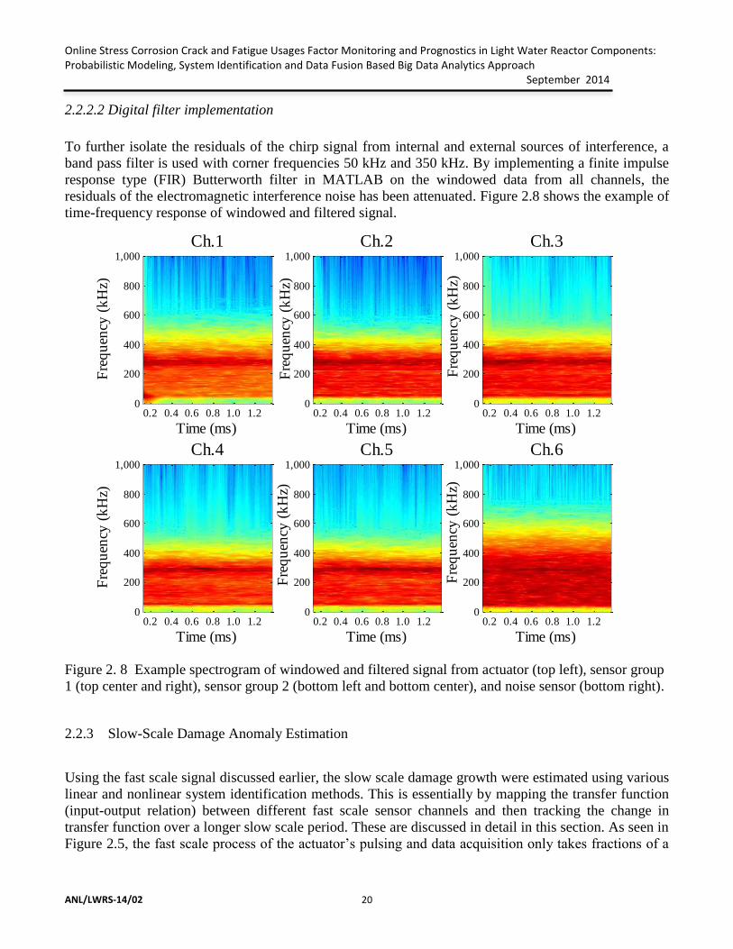
2.2.2.2 Digital filter implementation
To further isolate the residuals of the chirp signal from internal and external sources of interference, a
band pass filter is used with corner frequencies 50 kHz and 350 kHz. By implementing a finite impulse
response type (FIR) Butterworth filter in MATLAB on the windowed data from all channels, the
residuals of the electromagnetic interference noise has been attenuated. Figure 2.8 shows the example of
time-frequency response of windowed and filtered signal.
Figure 2. 8 Example spectrogram of windowed and filtered signal from actuator (top left), sensor group
1 (top center and right), sensor group 2 (bottom left and bottom center), and noise sensor (bottom right).
2.2.3 Slow-Scale Damage Anomaly Estimation
Using the fast scale signal discussed earlier, the slow scale damage growth were estimated using various
linear and nonlinear system identification methods. This is essentially by mapping the transfer function
(input-output relation) between different fast scale sensor channels and then tracking the change in
transfer function over a longer slow scale period. These are discussed in detail in this section. As seen in
Figure 2.5, the fast scale process of the actuator’s pulsing and data acquisition only takes fractions of a
Time (ms)
Fre
qu
ency
(k
Hz)
Ch.1
0.2 0.4 0.6 0.8 1.0 1.20
200
400
600
800
1,000
Time (ms)
Fre
qu
ency
(k
Hz)
Ch.2
0.2 0.4 0.6 0.8 1.0 1.20
200
400
600
800
1,000
Time (ms)
Fre
qu
ency
(k
Hz)
Ch.3
0.2 0.4 0.6 0.8 1.0 1.20
200
400
600
800
1,000
Time (ms)
Fre
qu
ency
(k
Hz)
Ch.4
0.2 0.4 0.6 0.8 1.0 1.20
200
400
600
800
1,000
Time (ms)
Fre
qu
ency
(k
Hz)
Ch.5
0.2 0.4 0.6 0.8 1.0 1.20
200
400
600
800
1,000
Time (ms)
Fre
qu
ency
(k
Hz)
Ch.6
0.2 0.4 0.6 0.8 1.0 1.20
200
400
600
800
1,000

Online Stress Corrosion Crack and Fatigue Usages Factor Monitoring and Prognostics in Light Water Reactor Components: Probabilistic Modeling, System Identification and Data Fusion Based Big Data Analytics Approach September 2014
ANL/LWRS-14/02
21
second to complete. In comparison, the slow scale predictor considers multiple data points separated by
time increments of 30 minutes. Consequently, the transfer function mapped between the input and
output signal during the fast scale process is assumed to be time invariant. However, during the slow
scale the estimated transfer function will not remain fixed and is expected to be time variant as the
system degrades structurally. As a result, the anomaly in the transfer function over the slow scale time
axis can be modeled and can be used to estimate the anomaly of the structure. General statistics and
linear system identification methods including correlation analysis, empirical transfer function
estimation [7], and Gaussian Process probabilistic modeling [8] are discussed in detail; These are used
individually for slow scale damage/anomaly trend time-series estimation.
2.2.3.1 Basic Scatter Plot Based Anomaly Analysis
The full signal and the filtered post-chirp data were compared over the life of the test structure. Figure
2.9 and Figure 2.10 display the scatter plots of both the full signal and the filtered windowed signal,
respectively. Each plot displays the data from the structure’s initial cycle and consecutive quarter lives.
Figure 2. 9 Scatter plot of first, quarter life, half-life, three quarters life, and end of life complete signal
from sensor group 1 (top left and top right) and sensor group 2 (bottom left and bottom right).
Only channels 4 and 5 in Figure 2.10 displayed an anomaly that the extremes of the signal were being
attenuated over the slow scale. However, this trend is not clear and could be due to a blind zone
discussed later. Also, sensors located away from the actuator (as in case of group 2 sensors refer Figure
2.2) are not always preferable due to requirement of more wiring and possibility of blind zone. If sensors
are placed away from the ultrasonic actuator a blind zone can be formed due to a crack between the
actuator and sensor. The blind zone may not allow the actuator signal to reach the sensor. If the sensor

Online Stress Corrosion Crack and Fatigue Usages Factor Monitoring and Prognostics in Light Water Reactor Components: Probabilistic Modeling, System Identification and Data Fusion Based Big Data Analytics Approach September 2014
ANL/LWRS-14/02 22
does not receive the signals it may not help to predict the correct anomaly even though the damage
actually continued growing. This can be seen from channels 4 and 5 data shown in Figure 2.10 that after
33 hours the signal amplitude remained constant after dropping significantly. Since inspection of the
scatter plots did not yield a substantial slow scale anomaly, more intensive methods of analysis were
necessary.
Figure 2. 10 Scatter plot of first, quarter life, half-life, three-quarters life, and end of life windowed and
filtered signal from sensor group 1 (top left and top right) and sensor group 2 (bottom left and right).
2.2.3.2 Single Channel Mean and Variance Based Anomaly Prediction
The means and variances of the sensor data were computed for each sample at every chirp cycle. Figure
2.11 and Figure 2.12 displays the plots of the means and variances, respectively, over the slow scale time
axis. From Figure 2.11, it can be seen that the mean of sensor signals from different channels do not
show any clear trend. Whereas from Figure 2.12 it can be seen that for channels 3, 4, and 5, the variance
shows an anomaly trend up to some extent as the structure degrades. However, the channel 2 variance
does not demonstrate such a relationship. In channels 4 and 5, the variance appears to change very little
after 35 hours which could be due to a possible blind zone developing due to through cracking of steam
generator pipe. A growing SCC crack through the surface of a structure would inhibit the signal from
being passed from the actuator to sensors of sensor group 2 (refer Figure 2.2). The attenuated signal
would decrease the overall variance in the signal and would not carry a complete picture of the overall
anomaly. Overall, the first order statistics fail to completely capture the desired relationship between
time and the structure’s degradation.

Online Stress Corrosion Crack and Fatigue Usages Factor Monitoring and Prognostics in Light Water Reactor Components: Probabilistic Modeling, System Identification and Data Fusion Based Big Data Analytics Approach September 2014
ANL/LWRS-14/02
23
Figure 2. 11 Calculated means from sensor group 1 (top right and top left) and sensor group 2 (bottom
right and bottom left).
0 10 20 30 40 50 60 700
0.5
1
1.5
2x 10
-5 Ch.2 Mean
Time (hours)
Mea
n (
Vo
lts)
0 10 20 30 40 50 60 700
0.5
1
1.5
2
2.5
3x 10
-5 Ch.3 Mean
Time (hours)
Mea
n (
Vo
lts)
0 10 20 30 40 50 60 70-3
-2.5
-2
-1.5
-1
-0.5
0
0.5
1
1.5x 10
-5 Ch.4 Mean
Time (hours)
Mea
n (
Vo
lts)
0 10 20 30 40 50 60 70-3.5
-3
-2.5
-2
-1.5
-1
-0.5
0
0.5x 10
-5 Ch.5 Mean
Time (hours)
Mea
n (
Vo
lts)

Online Stress Corrosion Crack and Fatigue Usages Factor Monitoring and Prognostics in Light Water Reactor Components: Probabilistic Modeling, System Identification and Data Fusion Based Big Data Analytics Approach September 2014
ANL/LWRS-14/02 24
Figure 2. 12 Calculated variances from sensor group 1 (top right and top left) and sensor group 2
(bottom right and bottom left).
2.2.3.3 Multi-Channel Covariance Base Damage Estimation
Since first order analysis using single sensor data failed to demonstrate a substantial consistent anomaly
trend prediction from each and every sensor channel, more intensive methods were necessary. Contrary
to mean and variance based single channel data analysis, the covariance was computed for each chirp
cycle between channels. The covariance for each cycle was plotted against the slow scale time axis and
examined for long term anomalies, illustrated in Figure 2.13 and Figure 2.14. From Figure 2.13, it can
be seen that, whenever a sensor channel measurement (from Ch. 2, 3, 4, and 5) was correlated with the
actuator channel data (Ch. 1), the covariance based anomaly time-series does not show any noteworthy
anomaly. The actuator channel may not capture more frequency content in the selected time-frequency
window although the actuator piezoelectric placed near to the sensor piezoelectric (Ch. 2 and 3) should
work ideally as a receiver after the pulsing is completed. The time-frequency plot shown in Figure 2.6
and Figure 2.8 supports this claim. Comparing channel 1 and 2’s time frequency plot, frequencies
0 10 20 30 40 50 60 705.6
5.8
6
6.2
6.4
6.6
6.8
7x 10
-3 Ch.2 Variance
Time (hours)
Var
ian
ce (
Vo
lts)
0 10 20 30 40 50 60 700.021
0.022
0.023
0.024
0.025
0.026
0.027
0.028
Ch.3 Variance
Time (hours)
Var
ian
ce (
Vo
lts)
0 10 20 30 40 50 60 701
2
3
4
5
6
7x 10
-3 Ch.4 Variance
Time (hours)
Var
ian
ce (
Vo
lts)
0 10 20 30 40 50 60 700.5
1
1.5
2
2.5
3
3.5
4x 10
-3 Ch.5 Variance
Time (hours)
Var
ian
ce (
Vo
lts)

Online Stress Corrosion Crack and Fatigue Usages Factor Monitoring and Prognostics in Light Water Reactor Components: Probabilistic Modeling, System Identification and Data Fusion Based Big Data Analytics Approach September 2014
ANL/LWRS-14/02
25
between 50 kHz and 350 kHz are significantly less prominent post-pulse in channel 1 than channel 2.
However, the covariance between sensor channels (2, 3, 4, and 5) shows some anomaly as shown in
Figure 2.14. On the other hand, it can be noticed from Figure 2.14 that if either or both of channel 4 and
5 are used the anomaly history does not show any clear trend other than the covariance between channel
2 and 4 and that is again up to first 30-35 hours. In addition, using these channels, it is observed that
there is not much change in anomaly trend after 30-35 hours, which could be due to the development of
a blind zone.
Figure 2. 13 Covariance between actuator and sensor group 1 (top right and top left) and actuator and
sensor group 2 (bottom right and bottom left).
0 10 20 30 40 50 60 70-9
-8.5
-8
-7.5
-7
-6.5
-6x 10
-4 Ch.1 and Ch.2 Covariance
Time (hours)
Co
var
ian
ce (
Vo
lts)
0 10 20 30 40 50 60 70
1.4
1.5
1.6
1.7
1.8
1.9
2
2.1
2.2x 10
-3 Ch.1 and Ch.3 Covariance
Time (hours)
Co
var
ian
ce (
Vo
lts)
0 10 20 30 40 50 60 70-0.5
0
0.5
1
1.5
2
2.5
3x 10
-4 Ch.1 and Ch.4 Covariance
Time (hours)
Co
var
ian
ce (
Vo
lts)
0 10 20 30 40 50 60 70-10
-8
-6
-4
-2
0
2
4x 10
-5 Ch.1 and Ch.5 Covariance
Time (hours)
Co
var
ian
ce (
Vo
lts)

Online Stress Corrosion Crack and Fatigue Usages Factor Monitoring and Prognostics in Light Water Reactor Components: Probabilistic Modeling, System Identification and Data Fusion Based Big Data Analytics Approach September 2014
ANL/LWRS-14/02 26
Figure 2. 14 Covariance between sensor group 1 and sensor group 2.
0 10 20 30 40 50 60 70-0.0115
-0.011
-0.0105
-0.01
-0.0095
-0.009
-0.0085
Ch.2 and Ch.3 Covariance
Time (hours)
Co
var
ian
ce (
Vo
lts)
0 10 20 30 40 50 60 70-1.4
-1.2
-1
-0.8
-0.6
-0.4
-0.2
0x 10
-3 Ch.2 and Ch.4 Covariance
Time (hours)
Co
var
ian
ce (
Vo
lts)
0 10 20 30 40 50 60 70-1
-0.5
0
0.5
1
1.5
2
2.5
3
3.5x 10
-4 Ch.2 and Ch.5 Covariance
Time (hours)
Co
var
ian
ce (
Vo
lts)
0 10 20 30 40 50 60 70-4
-2
0
2
4
6
8
10x 10
-4 Ch.3 and Ch.4 Covariance
Time (hours)
Co
var
ian
ce (
Vo
lts)
0 10 20 30 40 50 60 70-5
-4
-3
-2
-1
0
1
2
3x 10
-4 Ch.3 and Ch.5 Covariance
Time (hours)
Co
var
ian
ce (
Vo
lts)
0 10 20 30 40 50 60 70-12
-10
-8
-6
-4
-2x 10
-4 Ch.4 and Ch.5 Covariance
Time (hours)
Co
var
ian
ce (
Vo
lts)

Online Stress Corrosion Crack and Fatigue Usages Factor Monitoring and Prognostics in Light Water Reactor Components: Probabilistic Modeling, System Identification and Data Fusion Based Big Data Analytics Approach September 2014
ANL/LWRS-14/02
27
2.2.3.4 Linear Regression Based Damage Estimation
There are multiple linear system identification based approaches were evaluated for anomaly time-series
estimation. In this subsection a linear regression based approach is discussed. This is based on the
assumption that there exists a transfer function (TF) mapping between individual sensor channel
measurements. This TF ideally would stay unchanged if there is no damage. However, if there is any
damage, the TF, which has to be recursively estimated, would also change. Tracing the change in
parameters of TF, the anomaly or damage time-series can be estimated in real time. This is the basic
motivation behind the approach discussed in this subsection and subsequent subsection.
For this purpose, the data was directly mapped across channels to determine a linear relationship
of the form
𝒚 = 𝑏1𝒙 + 𝑏0 (2. 3 )
where 𝑥 is the input signal, 𝑦 is the output signal, 𝑏1 is the regression line’s slope, and 𝑏0 is the offset.
The regression algorithm solves for the 𝑏𝑖=0,1 coefficients through the linear system of equations
[
𝑦1
𝑦2
⋮𝑦𝑛
] = [
11⋮1
𝑥1
𝑥2
⋮𝑥𝑛
] [𝑏0
𝑏1] ( 2.4 )
by using the linear least squares estimation. Figure 2.15 for example displays a scatter plot of channel 2
versus channel 3 and the computed best fit line. While the linear regression fails to completely depict the
relationship between the channels, it appears to indicate a general inverse relationship between channels.
Figure 2. 15 Sample scatter plot of mapping between sensors in group 1 with regression line.
-0.8 -0.6 -0.4 -0.2 0 0.2 0.4 0.6 0.8-1.5
-1
-0.5
0
0.5
1
1.5
Linear Regression Between Ch. 2 and Ch. 3
Ch. 2 (V)
Ch
. 3
(V
)
Signal
Regression Line

Online Stress Corrosion Crack and Fatigue Usages Factor Monitoring and Prognostics in Light Water Reactor Components: Probabilistic Modeling, System Identification and Data Fusion Based Big Data Analytics Approach September 2014
ANL/LWRS-14/02 28
The coefficients for each cycle’s best fit line were plotted over the slow scale time axis, illustrated in
Figure 2.16, Figure 2.17, and Figure 2.18. Except between Ch. 1 and 5 (Figure 2.17) and Ch. 4 and 5
(Figure 2.18), the offset coefficients, 𝑏0, for the linear mapping across any of the channels did not
demonstrate any notable anomalies over the slow scale time axis. Similarly, the slope coefficients, 𝑏1,
only for the linear mapping between channel 2 and 3 and channel 4 and 5 displayed a significant
anomaly, as exhibited in Figure 2.18. Moreover, the slope coefficient 𝑏1 based anomaly was only
observed on linear mapping between sensors on the same sensor group.
Figure 2. 16 Linear fit parameters (both 𝑏0 and 𝑏1) for mapping between actuator and sensor group 1.
0 10 20 30 40 50 60 70-0.15
-0.14
-0.13
-0.12
-0.11
-0.1
b1 of Linear Fit Between Ch. 1 and Ch. 2
Time (hours)
b1 (
V/V
)
0 10 20 30 40 50 60 700
0.005
0.01
0.015
0.02
b0 of Linear Fit Between Ch. 1 and Ch. 2
Time (hours)
b0 (
mV
)
0 10 20 30 40 50 60 700.22
0.24
0.26
0.28
0.3
0.32
0.34
b1 of Linear Fit Between Ch. 1 and Ch. 3
Time (hours)
b1 (
V/V
)
0 10 20 30 40 50 60 700
0.005
0.01
0.015
0.02
0.025
0.03
b0 of Linear Fit Between Ch. 1 and Ch. 3
Time (hours)
b0 (
mV
)

Online Stress Corrosion Crack and Fatigue Usages Factor Monitoring and Prognostics in Light Water Reactor Components: Probabilistic Modeling, System Identification and Data Fusion Based Big Data Analytics Approach September 2014
ANL/LWRS-14/02
29
Figure 2. 17 Linear fit parameters (both 𝑏0 and 𝑏1) for mapping between actuator and sensor group 2
0 10 20 30 40 50 60 70-0.005
0
0.005
0.01
0.015
0.02
0.025
0.03
0.035
0.04
b1 of Linear Fit Between Ch. 1 and Ch. 4
Time (hours)
b1 (
V/V
)
0 10 20 30 40 50 60 70-0.03
-0.025
-0.02
-0.015
-0.01
-0.005
0
0.005
0.01
0.015
b0 of Linear Fit Between Ch. 1 and Ch. 4
Time (hours)
b0 (
mV
)
0 10 20 30 40 50 60 70-15
-10
-5
0
5x 10
-3b
1 of Linear Fit Between Ch. 1 and Ch. 5
Time (hours)
b1 (
V/V
)
0 10 20 30 40 50 60 70-0.035
-0.03
-0.025
-0.02
-0.015
-0.01
-0.005
0
0.005
b0 of Linear Fit Between Ch. 1 and Ch. 5
Time (hours)
b0 (
mV
)

Online Stress Corrosion Crack and Fatigue Usages Factor Monitoring and Prognostics in Light Water Reactor Components: Probabilistic Modeling, System Identification and Data Fusion Based Big Data Analytics Approach September 2014
ANL/LWRS-14/02 30
Figure 2. 18 Linear fit parameters (both 𝑏0 and 𝑏1) for mapping between sensors in group 1 (top) and
sensors in group 2 (bottom).
Furthermore, using the anomaly observed in the linear regression parameter, 𝑏1, the normalized anomaly
trend estimated with respect to the healthy state regression line slope (i.e. 𝑏10) and using the following
root square deviation form:
𝐴𝑛 = √(𝑏1𝑛
− 𝑏10)2
𝑏102 ( 2.5 )
where 𝐴𝑛 is the damage index at the 𝑛𝑡ℎ point in the slow scale time axis. The plots of the computed
damage indices for the linear mappings between Ch. 2 and 3 and Ch. 4 and 5 are displayed in Figure
2.19 and Figure 2.20, respectively. Both damage indices show strong anomalies over the slow scale
time axis. However, both plots demonstrate undesirable features, namely the large valleys between 30-
50 hours in the damage index of Ch. 2 and 3 and the damage decline after 50 hours in the damage index
of Ch. 4 and 5.
0 10 20 30 40 50 60 70-1.75
-1.7
-1.65
-1.6
-1.55
-1.5
-1.45
-1.4
-1.35
b1 of Linear Fit Between Ch. 2 and Ch. 3
Time (hours)
b1 (
V/V
)
0 10 20 30 40 50 60 700.005
0.01
0.015
0.02
0.025
0.03
0.035
0.04
0.045
0.05
b0 of Linear Fit Between Ch. 2 and Ch. 3
Time (hours)
b0 (
mV
)
0 10 20 30 40 50 60 70-0.4
-0.35
-0.3
-0.25
-0.2
-0.15
-0.1
-0.05
b1 of Linear Fit Between Ch. 4 and Ch. 5
Time (hours)
b1 (
V/V
)
0 10 20 30 40 50 60 70-0.035
-0.03
-0.025
-0.02
-0.015
-0.01
-0.005
0
b0 of Linear Fit Between Ch. 4 and Ch. 5
Time (hours)
b0 (
mV
)

Online Stress Corrosion Crack and Fatigue Usages Factor Monitoring and Prognostics in Light Water Reactor Components: Probabilistic Modeling, System Identification and Data Fusion Based Big Data Analytics Approach September 2014
ANL/LWRS-14/02
31
Figure 2. 19 Plot of the damage index computed from linear mapping between sensors in group 1.
Figure 2. 20 Plot of the damage index computed from linear mapping between sensors in group 2.
0 10 20 30 40 50 60 700
0.05
0.1
0.15
0.2
0.25
0.3
0.35
Time (hours)
Dam
age
Ind
ex (
A n)
Damage Index for Mapping Between Ch. 2 and Ch. 3
0 10 20 30 40 50 60 700
0.5
1
1.5
2
2.5
3
3.5
4
4.5
Time (hours)
Dam
age
Ind
ex (
A n)
Damage Index for Mapping Between Ch. 4 and Ch. 5

Online Stress Corrosion Crack and Fatigue Usages Factor Monitoring and Prognostics in Light Water Reactor Components: Probabilistic Modeling, System Identification and Data Fusion Based Big Data Analytics Approach September 2014
ANL/LWRS-14/02 32
2.2.3.5 Correlation Analysis Based Damage Estimation
In addition to linear regression, correlation analysis (CRA) method (a type of linear system
identification, [7]) was also evaluated for the slow scale state estimator. Mapping across sensor signals
was also performed assuming a linear time invariant relation between the signals from individual
channels. For example, the signals from one channel can be assumed as the input, 𝑥(𝑡), and signals from
another channel can be assumed as the output, 𝑦(𝑡), and the transformation between these channels can
be expressed as:
𝑦(𝑡) = ∑ ℎ(𝑘)𝑥(𝑡 − 𝑘) + 𝑣(𝑡)
∞
𝑘=0
( 2.6 )
Where the correlation function between the input 𝑥(𝑡) output 𝑦(𝑡) is given by
𝑅𝑦𝑥(𝜏) = ∑ ℎ(𝑘)𝑅𝑥(𝜏 − 𝑘)
𝑀
𝑘=0
(2. 7 )
where 𝑅𝑦𝑥(𝜏) and 𝑅𝑥(𝜏) are the cross correlation and autocorrelation coefficients matrices obtained
from equations 7 ) and ( 2.9 ).
�̂�𝑦𝑥(𝜏) =1
𝑁∑ 𝑦(𝑡 + 𝜏)𝑥(𝑡)∗
𝑁−𝜏
𝑡=1
, 𝜏 = 0,1,2, … ( 2.8 )
�̂�𝑥𝑥(𝜏) =1
𝑁∑ 𝑥(𝑡 + 𝜏)𝑥(𝑡)∗
𝑁−𝜏
𝑡=1
𝜏 = 0,1,2, … ( 2.9 )
The correlation function can be alternatively written in matrix form as follows:
[ 𝑅𝑦𝑥(0)
𝑅𝑦𝑥(1)
⋮𝑅𝑦𝑥(𝑀)]
= [
𝑅𝑥(0)𝑅𝑥(−1)
⋮𝑅𝑥(−𝑀)
𝑅𝑥(1)𝑅𝑥(0)
⋮𝑅𝑥(−𝑀 + 1)
⋯⋯⋱⋯
𝑅𝑥(𝑀)𝑅𝑥(𝑀 − 1)
⋮𝑅𝑥(0)
] [
ℎ(0)ℎ(1)
⋮ℎ(𝑀)
] ( 2.10 )
Solving for the transfer function ℎ(𝑡) requires the autocorrelation matrix to be inverted, which is
computationally expensive for matrices of large dimensions. Accordingly, only the first 3,000 points of
the selected data were used for this method. Figure 2.21 displays the actual and predicted out from CRA
using channel 2 as the input and channel 3 as the output. Figure 2.22 displays the actual and predicted
out from CRA using channel 4 as the input and channel 5 as the output. Both predictions from CRA did

Online Stress Corrosion Crack and Fatigue Usages Factor Monitoring and Prognostics in Light Water Reactor Components: Probabilistic Modeling, System Identification and Data Fusion Based Big Data Analytics Approach September 2014
ANL/LWRS-14/02
33
not closely replicate the actual output. Consequently, CRA was observed not to be an appropriate
method for modeling this system.
Figure 2. 21 Predicted and actual output using CRA mapping between sensors in group 1.
Figure 2. 22 Prediction and actual output using CRA mapping between sensors in group 2.
0 0.25 0.5 0.75 1 1.25 1.5-1.5
-1
-0.5
0
0.5
1
1.5
Actual and Predicted Output Using CRA Approach
Time (ms)
Sig
nal
(V
)
Actual
Predicted
0 0.5 1 1.5-0.25
-0.2
-0.15
-0.1
-0.05
0
0.05
0.1
0.15
0.2
0.25
Actual and Predicted Output Using CRA Approach
Time (ms)
Sig
nal
(V
)
Actual
Predicted

Online Stress Corrosion Crack and Fatigue Usages Factor Monitoring and Prognostics in Light Water Reactor Components: Probabilistic Modeling, System Identification and Data Fusion Based Big Data Analytics Approach September 2014
ANL/LWRS-14/02 34
While the output prediction of CRA was not optimal, the damage index was still computed for the tests
using an absolute difference based formula. The damage index was computed according to the
expression:
𝐴𝑛 = |휀𝑛 − 휀0| (2.11 )
where 𝑛 is the chirp cycle number. 휀𝑛 is the ℓ2-norm of the prediction error defined by the following
expression:
휀𝑛 = √(𝑦𝑜𝑏1− 𝑦𝑝1
)2
+ (𝑦𝑜𝑏2− 𝑦𝑝2
)2
+ ⋯+ (𝑦𝑜𝑏𝑖− 𝑦𝑝𝑖
)2
( 2.12 )
where 𝑦𝑜𝑏𝑖 is the observed output of the system and 𝑦𝑝𝑖
is the predicted output of the system at point 𝑖 in
the 𝑛𝑡ℎ chirp cycle. The damage index was computed for the CRA method on mappings between
channels 2 and 3 and channels 4 and 5. The plots of 𝐴𝑛 over the slow scale axis are displayed in Figure
2.23 and Figure 2.24. CRA mapping between Ch. 2 and 3 did not demonstrate a substantial slow scale
anomaly. The computed damage index contained a significant component of noise. The damage index
between Ch. 4 and 5 demonstrated an anomaly up to 25 hours, but did not reflect and damage growth
thereafter. Additionally, this damage index displayed significant noise throughout the slow scale axis.
As a result, the CRA method does not effectively describe the system or the damage growth within the
system.
Figure 2. 23 Computed damage index from CRA mapping between sensors in group 1.
0 10 20 30 40 50 60 700
0.2
0.4
0.6
0.8
1
1.2
1.4
Damage Index for Ch. 2 and 3
Time (hours)
Dam
age
Ind
ex (
A n)

Online Stress Corrosion Crack and Fatigue Usages Factor Monitoring and Prognostics in Light Water Reactor Components: Probabilistic Modeling, System Identification and Data Fusion Based Big Data Analytics Approach September 2014
ANL/LWRS-14/02
35
Figure 2. 24 Computed damage index from CRA mapping between sensors in group 2.
2.2.3.6 Empirical Transfer Function Estimation Based Damage Estimation
In addition, another linear system identification technique known as empirical transfer function
estimation (ETFE), [7] was also evaluated for the time series anomaly trend estimation. Linear mapping
was performed across channels using the ETFE. With this approach, the relationship between the input
and output channels is identified by the following system equation:
𝒚 = 𝑃𝑛(𝑗𝜔)𝒙 (2.13 )
In this equation, the transfer function, 𝑃𝑛(𝑗𝜔), is expressed as:
𝑃𝑛(𝑗𝜔) =𝑆𝑥𝑦
𝑛 (𝑗𝜔)
𝑆𝑥𝑥𝑛 (𝑗𝜔)
( 2.14 )
where 𝑆𝑥𝑦𝑛 (𝑗𝜔) and 𝑆𝑥𝑥
𝑛 (𝑗𝜔) are the cross-spectral power densities and auto-spectral power densities
respectively. The spectral densities are calculated using the cross-covariance coefficients, 𝐶𝑥𝑦𝑛 (𝑚), and
auto-covariance coefficients, 𝐶𝑥𝑥𝑛 , as follows:
𝑆𝑥𝑦𝑛 (𝑗𝜔) = ∑ 𝐶𝑥𝑦
𝑛 𝜔(𝑘)𝑒−𝑗𝜔𝑘
𝑀
𝑘=−𝑀
( 2.15 )
0 10 20 30 40 50 60 700
0.1
0.2
0.3
0.4
0.5
0.6
0.7
0.8
0.9
Damage Index for Ch. 4 and 5
Time (hours)
Dam
age
Ind
ex (
A n)

Online Stress Corrosion Crack and Fatigue Usages Factor Monitoring and Prognostics in Light Water Reactor Components: Probabilistic Modeling, System Identification and Data Fusion Based Big Data Analytics Approach September 2014
ANL/LWRS-14/02 36
𝑆𝑥𝑥𝑛 (𝑗𝜔) = ∑ 𝐶𝑥𝑥
𝑛 𝜔(𝑘)𝑒−𝑗𝜔𝑘
𝑀
𝑘=−𝑀
( 2.16 )
where 𝜔(𝑘) is the lag window used to smoothen the data and 𝑀 is the trimming parameter for the
window. Using the ETFE method, the transfer function was computed and the output channel was
predicted and compared to the actual output data. In Figure 2.25, channel 2 was used as the input
channel and channel 3 was used as the output channel. The plot overlays the predicted output over the
actual output. The resulting response did not closely follow the actual output of the channel. Similarly,
in Figure 2.26, channel 4 was used as the input and channel 5 was used as the output. The resulting
predicted output was plotted on top of the actual output. Accordingly, the ETFE method did not closely
predict a response close to the actual output. Consequently, the empirical transfer function estimation
method was concluded to not be an appropriate method to identify the system.
Figure 2. 25 Predicted and actual output using ETFE mapping between sensors in group 1.
0 0.25 0.5 0.75 1 1.25 1.5-0.8
-0.6
-0.4
-0.2
0
0.2
0.4
0.6
0.8
Actual and Predicted Output Using ETFE Approach
Time (ms)
Sig
nal
(V
)
Actual
Predicted

Online Stress Corrosion Crack and Fatigue Usages Factor Monitoring and Prognostics in Light Water Reactor Components: Probabilistic Modeling, System Identification and Data Fusion Based Big Data Analytics Approach September 2014
ANL/LWRS-14/02
37
Figure 2. 26 Predicted and actual output using ETFE mapping between sensors in group 2.
While the output prediction of ETFE was not optimal, the damage index was still computed for the tests
using a root square deviation based formula. The damage index was computed using the prediction error
according to the formulas in equation 2.11 and Eq. 2.12. Both computed indices demonstrate erratic
behaviors. The mapping between Ch. 2 and 3 (refer Figure 2.27) did not present an underlying anomaly
and demonstrated significant components of noise. The damage index computed for the mapping
between Ch. 4 and 5 (refer Figure 2.28) presents an underlying anomaly but has a significant amount of
oscillations. Moreover, this damage index does not grow after 40 hours, indicating a blind zone
forming. In summary, ETFE was not able to effectively describe the system or capture the overall
damage growth within the system effectively.
0 0.25 0.5 0.75 1 1.25 1.5-0.4
-0.3
-0.2
-0.1
0
0.1
0.2
0.3
0.4
Actual and Predicted Output Using ETFE Approach
Time (ms)
Sig
nal
(V
)
Actual
Predicted

Online Stress Corrosion Crack and Fatigue Usages Factor Monitoring and Prognostics in Light Water Reactor Components: Probabilistic Modeling, System Identification and Data Fusion Based Big Data Analytics Approach September 2014
ANL/LWRS-14/02 38
Figure 2. 27 Computed damage index from ETFE mapping between sensors in group 1.
Figure 2. 28 Computed damage index from ETFE mapping between sensors in group 2.
0 10 20 30 40 50 60 700
0.5
1
1.5
2
2.5
3
Damage Index for Ch. 2 and 3
Time (hours)
Dam
age
Ind
ex (
A n)
0 10 20 30 40 50 60 700
0.5
1
1.5
2
2.5
Damage Index for Ch. 4 and 5
Time (hours)
Dam
age
Ind
ex (
A n)

Online Stress Corrosion Crack and Fatigue Usages Factor Monitoring and Prognostics in Light Water Reactor Components: Probabilistic Modeling, System Identification and Data Fusion Based Big Data Analytics Approach September 2014
ANL/LWRS-14/02
39
2.2.3.7 Bayesian Forecasting with Gaussian Process Based Damage Estimation
In addition to the linear system identification techniques, nonlinear techniques were evaluated for the
slow scale state estimator. Nonlinear estimation was performed across channels using a Bayesian
forecasting approach [1,8]. The goal of the forecasting approach is to compute the posterior distribution
of the test output, 𝑦𝑛+1. The framework accomplishes the prediction by using a random test input, 𝑥𝑛+1,
a set of 𝑛 training data points, 𝑫 = {𝑥𝑖 , 𝑦𝑖}𝑖=1,…,𝑛, and prescribed likelihood and noise functions. The
likelihood function can be defined as a prior over the space of possible functions to model the random
output by 𝑓(𝑦𝑖|𝛼; 𝑖 = 1,2, … , 𝑛 + 1). Additionally, the noise function can be described as a prior over
the noise, 𝑓(𝜗|𝛽), where 𝜗 is an appropriate noise vector that accounts for electrical and physical
sources of noise within the specimen. With these factors prescribed, the conditional probability of
system as described by the probabilistic model can be written as follows:
𝑓(𝑦𝑛+1|{𝑥𝑖=1,…,𝑛, 𝛼, 𝛽}) = ∫(𝑦𝑛+1|{𝑥𝑖=1,…,𝑛, 𝑦, 𝜗}) 𝑓(𝑎|𝛼)𝑓(𝜗|𝛽)𝑑𝑎 𝑑𝜗 ( 2.17 )
The integral in Eq. 2.17 is nontrivial to evaluate. Various methods have been developed to
compute the integral including evidence maximization and Monte Carlo simulation. Accordingly, the
integral becomes much simpler to evaluate if the underlying function of the signal is governed by a
Gaussian distribution. Consequently, the exact analytical form can be written as follows:
𝑓(𝑦𝑛+1|{𝑥𝑖=1,…,𝑛}, 𝑲𝑛+1) =1
(2𝜋)𝑛+1/2|𝑲𝑛+1|1/2
𝑒−12(𝑦𝑛+1−𝜇)𝑇𝑲𝑛+1
−1 (𝑦𝑛+1−𝜇) (2.18 )
where 𝜇 is the function mean and 𝐾𝑛 is a 𝑛x𝑛 kernel matrix. The kernel matrix is computed from the
parameterized kernel function described in a later section. Simplifying this expression under the
assumption of a function mean of zero, the form can be written as follows:
𝑓(𝑦𝑛+1|{𝑥𝑖 , 𝑦𝑖}, 𝑥𝑛+1, 𝑘𝑖𝑗(𝑥𝑖, 𝑥𝑗 , 𝚯)𝑖,𝑗=1,2,…,𝑛) = √|𝑲𝑛|
(2𝜋)|𝑲𝑛+1|𝑒
−(𝑦𝑛+1−�̂�𝑛+1)2
2𝜎�̂�𝑛+12
(2.19)
where �̂�𝑛+1 is the next step mean prediction at the output signal data point, 𝑛 + 1. The next step
predicted mean can be computed by:
�̂�𝑛+1 = 𝒌𝑇𝑲𝑛−1𝒚𝑛; 𝑘𝑖 = 𝑘(𝑥𝑛+1, 𝑥𝑖)𝑖=1,2,…,𝑛 (2.20 )
Similarly, 𝜎�̂�𝑛+1
2 is the next step predicted variance at the output signal data point, 𝑛 + 1, which can be
evaluated by:
𝜎�̂�𝑛+1
2 = 𝛋 − 𝒌𝑇𝑲𝑛−1𝒌; 𝑘𝑖 = 𝑘(𝑥𝑛+1, 𝑥𝑖)𝑖=1,2,…,𝑛; 𝛋 = k(𝑥𝑛+1, 𝑥𝑛+1) (2.21 )
There are many options available for prior interpolating kernel functions. The selected kernel should
reflect the assumptions made about the process being modeled. More generally, a kernel function is

Online Stress Corrosion Crack and Fatigue Usages Factor Monitoring and Prognostics in Light Water Reactor Components: Probabilistic Modeling, System Identification and Data Fusion Based Big Data Analytics Approach September 2014
ANL/LWRS-14/02 40
required to generate a positive definite kernel matrix for any set of inputs. In this instance, a kernel was
created by combining the Gaussian likelihood function to model the signal and the additive
measurement noise function to model the noise. The Gaussian likelihood function [8] is written as
follows:
𝑘𝑙(𝑦𝑖|𝑥𝑖 , 𝜃𝑙2) =
1
√2𝜋𝜃𝑙2𝑒
−−𝑥𝑖
2
2𝜃𝑙2
(2.22 )
where 𝜃𝑙 is the likelihood hyperparameter. Similarly, the additive measurement noise function can be
described as the following covariance function:
𝑘𝑐(𝑥𝑖 , 𝑥𝑗) = 𝜃𝑐2𝛿(𝑥𝑖 − 𝑥𝑗) (2.23 )
where 𝜃𝑐 is the scatter hyperparameter. These functions were combined to form the kernel as follows:
𝑘(𝑥𝑖 , 𝑥𝑗 , Θ) = 1
√2𝜋𝜃𝑙2𝑒
−−𝑥𝑖
2
2𝜃𝑙2
+ 𝜃𝑐2𝛿(𝑥𝑖 − 𝑥𝑗) (2.24 )
All of these Gaussian process proceedings have discussed characteristics of the probability model for
fixed hyperparameters. However, to obtain the proper values for these hyperparameters, optimization
must be performed. Using a fixed training data set, 𝐷 = {𝑥𝑖 , 𝑦𝑖}𝑖=1,…,𝑛, the hyperparameters can be
estimated by minimizing the following log likelihood:
𝐿 = log (𝑓(Θ|𝐷 = {𝑥𝑖 , 𝑦𝑖}𝑖=1,2…𝑚, K(∙))) = −1
2log (det (𝐾)) −
1
2x𝑇K−1x −
𝜇
2log (2𝜋) (2.25)
From the log likelihood equation, hyperparameters can be determined through optimization procedures
such as Polak and Ribiere nonlinear conjugate gradient method. The method is initialized by selecting a
starting value for the hyperparameter, 𝜃, and a step direction, 𝑝𝑘. Next, a line search is performed to
determine 𝑤𝑗 such that 𝜃𝑗+1 = 𝜃𝑗 + 𝑤𝑗𝑝𝑗. Next, the algorithm computes the following equations:
𝜓𝑗+1 =𝑔𝑗+1
𝑇 (𝑔𝑗+1 − 𝑔𝑖)
𝑔𝑗𝑇𝑔𝑗
(2.26)
where 𝑔𝑗 = ∇𝑓(𝜃𝑗+1) and
𝑝𝑗+1 = −𝑔𝑗 + 𝜓𝑗+1𝑝𝑗 (2.27 )
The algorithm loops, incrementing 𝑗 until ‖𝑔𝑗‖ < 1. Thereafter, the value of 𝜃 when the loop is exited is
the optimized hyperparameter. The above discussed GP was used in two ways to predict the anomaly
trend. First, at any given time with the selected input and output channel data the hyperparameters were
estimated and compared over time to check if there is any trend or not. Second, for the given input and
output channels the respective model parameters (here the hyperparameters) were estimated at the health

Online Stress Corrosion Crack and Fatigue Usages Factor Monitoring and Prognostics in Light Water Reactor Components: Probabilistic Modeling, System Identification and Data Fusion Based Big Data Analytics Approach September 2014
ANL/LWRS-14/02
41
condition of the structure and these fixed hyperparameters were used to predict the output channel data
for a given input channel data at any given time. Then, this predicted and actual output data is used to
predict the error signals and associated damage index using equation (2.11) and equation (2.12). In both
the above mentioned cases the purpose of GP model is to accurately model the input-output relation
such that the predicted output best matches the actual output. For example, Figure 2.29 (top plot)
displays the predicted channel 3 output and associated 2𝜎 error bounds with respect to channel 2 data as
input signals. Figure 2.29 (bottom plot) shows the comparison of mean predicted channel 3 output with
actual measured output. Figure 2.30, top and bottom plots, shows the magnified version of Figure 2.29,
top and bottom plots, respectively. Additionally, Figure 2.31 (top plot) displays the predicted channel 5
output and associated 2𝜎 error bounds with respect to channel 4 data as input signals. Figure 2.31
(bottom plot) shows the comparison of mean predicted channel 5 output with actual measured output.
Figure 2.32 top and bottom plots, shows the magnified version of Figure 2.31, top and bottom plots,
respectively. The figures show that the mappings depict a significant improvement in the quality of fit
when comparted to the linear system identification models.
Figure 2. 29 Predicted output with two standard deviation error bounds (top) and predicted and actual
output from mapping between sensors in group 1 (bottom).
0 0.05 0.1 0.15 0.2 0.25 0.3 0.35 0.4 0.45 0.5-1.5
-1
-0.5
0
0.5
1
1.5
Predicted Ch. 3 Output Using Ch. 2 as Input
Time (ms)
Sig
nal
(V
)
2 Error Bounds
Predicted
0 0.05 0.1 0.15 0.2 0.25 0.3 0.35 0.4 0.45 0.5-1.5
-1
-0.5
0
0.5
1
1.5
Time (ms)
Sig
nal
(V
)
Predicted Output and Actual Output for Ch.3
Actual
Predicted

Online Stress Corrosion Crack and Fatigue Usages Factor Monitoring and Prognostics in Light Water Reactor Components: Probabilistic Modeling, System Identification and Data Fusion Based Big Data Analytics Approach September 2014
ANL/LWRS-14/02 42
Figure 2. 30 Magnified version of Figure 2.29.
Figure 2. 31 Predicted output with two standard deviation error bounds (top) and predicted and actual
output from mapping between sensors in group 2 (bottom).
0.025 0.03 0.035 0.04 0.045
-1
-0.5
0
0.5
1
Predicted Ch.3 Output Using Ch. 2 as Input
Time (ms)
Sig
nal
(V
)
2 Error Bounds
Predicted
0.025 0.03 0.035 0.04 0.045
-1
-0.5
0
0.5
1
Time (ms)
Sig
nal
(V
)
Predicted Output and Actual Output for Ch.3
Actual
Predicted
0 0.05 0.1 0.15 0.2 0.25 0.3 0.35 0.4 0.45 0.5-0.2
-0.15
-0.1
-0.05
0
0.05
0.1
0.15
0.2
Predicted Ch.5 Output Using Ch. 4 as Input
Time (ms)
Sig
nal
(V
)
2 Error Bounds
Predicted
0 0.05 0.1 0.15 0.2 0.25 0.3 0.35 0.4 0.45 0.5-0.2
-0.15
-0.1
-0.05
0
0.05
0.1
0.15
0.2
Time (ms)
Sig
nal
(V
)
Predicted Output and Actual Output for Ch.5
Actual
Predicted

Online Stress Corrosion Crack and Fatigue Usages Factor Monitoring and Prognostics in Light Water Reactor Components: Probabilistic Modeling, System Identification and Data Fusion Based Big Data Analytics Approach September 2014
ANL/LWRS-14/02
43
Figure 2. 32 Magnified version of Figure 2.31.
Once the mapping between the input and output signals was established at a given instant, the
corresponding anomaly trend was estimated using the above mentioned two approaches. The respective
results are discussed below:
Approach-1:
For the first approach of the Gaussian Process based anomaly trend prediction the hyperparameters for
each Gaussian Process mapping were plotted over the slow scale time axis. Figure 2.33 depicts the
hyperparameters for the mapping between Ch. 2 and 3 and Figure 2.34 depicts the hyperparameters for
the mapping between Ch. 4 and 5. In both Gaussian Process mappings, the scatter hyperparameter, 𝜃𝑐,
demonstrates significantly better anomaly trend over the slow scale time axis compared to the likelihood
hyperparameter, 𝜃𝑙. To note that the hyperparameter (𝜃𝑐) capture the scatter between the input-output
mapping. It is assumed as the structural damage grows due to small microstructural defect there would
be more ultrasonic signal reflections or anomaly. This increasing anomaly in form of ultrasonic
reflections is ideally to be captured by the scatter hyperparameter. In both cases, the likelihood
parameter is much smaller than the scatter hyperparameters. A weighted combination of these
hyperparameters to create a hybrid damage index will result in the scatter hyperparameter dominating
the overall shape of the damage index.
0.025 0.03 0.035 0.04 0.045
-0.1
-0.05
0
0.05
0.1
0.15
Predicted Ch.5 Output Using Ch. 4 as Input
Time (ms)
Sig
nal
(V
)
2 Error Bounds
Predicted
0.025 0.03 0.035 0.04 0.045
-0.1
-0.05
0
0.05
0.1
0.15
Time (ms)
Sig
nal
(V
)
Predicted Output and Actual Output for Ch.5
Actual
Predicted

Online Stress Corrosion Crack and Fatigue Usages Factor Monitoring and Prognostics in Light Water Reactor Components: Probabilistic Modeling, System Identification and Data Fusion Based Big Data Analytics Approach September 2014
ANL/LWRS-14/02 44
Figure 2. 33 Hyperparameters for Gaussian Process model computed between sensors in group 1.
Figure 2. 34 Hyperparameters for Gaussian Process model computed between sensors in group 2.
The ℓ2-norm of each pair of hyperparameters was computed and plotted over the slow scale. Figure 2.35
and Figure 2.36 display the ℓ2-norm of the hyperparameters for Ch. 2 and 3 and Ch. 4 and 5,
respectively. Both plots take a similar form of the scatter hyperparameters plot since it is much larger
than the likelihood hyperparameter. Additionally, the scatter hyperparameter of Ch. 2 and 3 is much
larger than that of Ch. 4 and 5.
0 10 20 30 40 50 600.06
0.062
0.064
0.066
0.068
0.07
0.072
0.074
0.076
c
Time (hours)
c for Fit between Ch.2 and Ch.3
0 10 20 30 40 50 60
9.988
9.99
9.992
9.994
9.996
9.998
10
10.002
10.004
10.006
10.008
x 10-4
l
Time (hours)
l for Fit between Ch.2 and Ch.3
0 10 20 30 40 50 60
1.4
1.6
1.8
2
2.2
2.4
2.6
2.8
3
3.2
3.4
x 10-3
c
Time (hours)
c for Fit between Ch.4 and Ch.5
0 10 20 30 40 50 60
9.998
9.9985
9.999
9.9995
10
x 10-4
l
Time (hours)
l for Fit between Ch.4 and Ch.5

Online Stress Corrosion Crack and Fatigue Usages Factor Monitoring and Prognostics in Light Water Reactor Components: Probabilistic Modeling, System Identification and Data Fusion Based Big Data Analytics Approach September 2014
ANL/LWRS-14/02
45
Figure 2. 35 ℓ2-norm of hyperparameters computed between sensors in group 1.
Figure 2. 36 ℓ2-norm of hyperparameters computed between sensors in group 2.
0 10 20 30 40 50 600.06
0.062
0.064
0.066
0.068
0.07
0.072
0.074
0.076
l2-n
orm
of
Time (hours)
l2-norm of Hyperparameters for Fit between Ch.2 and Ch.3
0 10 20 30 40 50 60
1.8
2
2.2
2.4
2.6
2.8
3
3.2
3.4
3.6
x 10-3
l2-n
orm
of
Time (hours)
l2-norm of Hyperparameters for Fit between Ch.4 and Ch.5
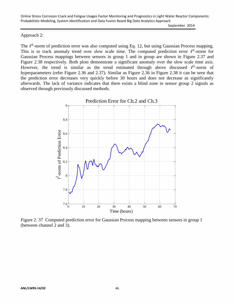
Online Stress Corrosion Crack and Fatigue Usages Factor Monitoring and Prognostics in Light Water Reactor Components: Probabilistic Modeling, System Identification and Data Fusion Based Big Data Analytics Approach September 2014
ANL/LWRS-14/02 46
Approach 2:
The ℓ2-norm of prediction error was also computed using Eq. 12, but using Gaussian Process mapping.
This is to track anomaly trend over slow scale time. The computed prediction error ℓ2-norm for
Gaussian Process mappings between sensors in group 1 and in group are shown in Figure 2.37 and
Figure 2.38 respectively. Both plots demonstrate a significant anomaly over the slow scale time axis.
However, the trend is similar as the trend estimated through above discussed ℓ2-norm of
hyperparameters (refer Figure 2.36 and 2.37). Similar as Figure 2.36 in Figure 2.38 it can be seen that
the prediction error decreases very quickly before 30 hours and does not decrease as significantly
afterwards. The lack of variance indicates that there exists a blind zone in sensor group 2 signals as
observed through previously discussed methods.
Figure 2. 37 Computed prediction error for Gaussian Process mapping between sensors in group 1
(between channel 2 and 3).
0 10 20 30 40 50 60 707.6
7.8
8
8.2
8.4
8.6
8.8
9
Time (hours)
l2-n
orm
of
Pre
dic
tio
n E
rro
r
Prediction Error for Ch.2 and Ch.3
0 10 20 30 40 50 60 701.1
1.2
1.3
1.4
1.5
1.6
1.7
1.8
1.9
Time (hours)
l2-n
orm
of
Pre
dic
tio
n E
rro
r
Prediction Error for Ch.4 and Ch.5

Online Stress Corrosion Crack and Fatigue Usages Factor Monitoring and Prognostics in Light Water Reactor Components: Probabilistic Modeling, System Identification and Data Fusion Based Big Data Analytics Approach September 2014
ANL/LWRS-14/02
47
Figure 2. 38 Computed prediction error for Gaussian Process mapping between sensors in group 2
(between channel 4 and 5).
In addition, from the prediction error 𝓵𝟐-norm, an equivalent healthy state referenced damage index was
also computed for the Gaussian Process mappings using Eq. 2.11. The plots of the damage index for the
mapping between Ch. 2 and 3 and Ch. 4 and 5 depicted in Figure 2.39 and Figure 2.40, respectively.
Unlike Figure 2.37 and 2.38, in both cases, the damage indices demonstrate upward anomaly trends.
However, they also demonstrate the same undesirable characteristics (e.g. local valleys) as the prediction
error plots discussed in previous sections. Consequently, these recurrent issues are due to the sensor
configuration on the specimen. The configuration appears to limit the amount of information each sensor
is able to receive since blind zones and other impediments are formed during damage growth. As a
result, the implementation of a multi-node data fusion technique is necessary to obtain a complete
description of the overall anomaly. This is discussed below.
0 10 20 30 40 50 60 707.6
7.8
8
8.2
8.4
8.6
8.8
9
Time (hours)
l2-n
orm
of
Pre
dic
tio
n E
rro
r
Prediction Error for Ch.2 and Ch.3
0 10 20 30 40 50 60 701.1
1.2
1.3
1.4
1.5
1.6
1.7
1.8
1.9
Time (hours)
l2-n
orm
of
Pre
dic
tio
n E
rro
r
Prediction Error for Ch.4 and Ch.5

Online Stress Corrosion Crack and Fatigue Usages Factor Monitoring and Prognostics in Light Water Reactor Components: Probabilistic Modeling, System Identification and Data Fusion Based Big Data Analytics Approach September 2014
ANL/LWRS-14/02 48
Figure 2. 39 Computed baseline referenced damage index for Gaussian Process mapping between
sensors in group 1 (between channel 2 and 3).
Figure 2. 40 Computed baseline referenced damage index for Gaussian Process mapping between
sensors in group 2 (between channel 4and 5).
0 10 20 30 40 50 60 700
0.1
0.2
0.3
0.4
0.5
0.6
0.7
0.8
0.9
1
Time (hours)
Dam
ae I
ndex
(A n)
Damage Index for Ch.2 and Ch.3
0 10 20 30 40 50 60 700
0.1
0.2
0.3
0.4
0.5
0.6
0.7
Time (hours)
Dam
ae I
nd
ex (
A n)
Damage Index for Ch.4 and Ch.5

Online Stress Corrosion Crack and Fatigue Usages Factor Monitoring and Prognostics in Light Water Reactor Components: Probabilistic Modeling, System Identification and Data Fusion Based Big Data Analytics Approach September 2014
ANL/LWRS-14/02
49
2.2.4 Multi-Node Sensor Data Fusion
Since the system identification methods presented in earlier sections alone fail to demonstrate a
complete picture of the structural degradation from a single pair of sensor channels, multi-node data
fusion is necessary. Dimension reduction through principal component analysis (PCA) was chosen as
the method for sensor fusion. PCA identifies the direction of the principal components where the
variance in changes in dynamics is a maximum. To perform PCA on the damage indices, the data path
depicted in Figure 2.41 was implemented. First, consecutive channels were mapped using the Gaussian
Process as discussed earlier. From these Gaussian Process mappings, the damage index for each pair of
channels was computed using the prediction error method in equations (2.11) and (2.12). Next, these
damage indices were processed using PCA dimension reduction technique where the final damage index
is computed along the direction of the first principal component.
Figure 2. 41 A diagram of the data path for PCA dimension reduction.
To perform PCA, the damage index time series matrix was generated according to the following
expression:
𝑨 = [𝑨𝟏𝟐 𝑨𝟐𝟑 𝑨𝟑𝟒 𝑨𝟒𝟓] (2.28 )

Online Stress Corrosion Crack and Fatigue Usages Factor Monitoring and Prognostics in Light Water Reactor Components: Probabilistic Modeling, System Identification and Data Fusion Based Big Data Analytics Approach September 2014
ANL/LWRS-14/02 50
where 𝐴𝑖𝑗 is the damage index computed from the Gaussian Process mapping between Ch. 𝑖 and Ch. 𝑗.
From the 𝑨 matrix, the covariance matrix, 𝑪𝑨, is computed. With the covariance matrix, the principal
components can be computed by solving the eigenvalue problem:
𝝀𝒗 = 𝑪𝑨𝒗 (2.29 )
where the size of the eigenvalue 𝝀 corresponding to an eigenvector 𝒗 of covariance matrix 𝑪𝑨 equals the
variance in the direction 𝑣. With these values, a transformation can be obtained to fuse the damage index
matrix, 𝑨, into a single damage index time series. The transformation can be defined as the following:
𝑨∗ = 𝑨𝒎𝒙𝒏𝚽𝒏𝒙𝟏 (2.30 )
where 𝑚 is the number of measurement points at a given instant and 𝑛 is the number of cross sensor
channel mappings. Also, 𝚽 is the vector containing the principal component weights and 𝐴∗ is the new
damage index vector for the system. Figure 2.42 displays the damage index time series of the Gaussian
Process mappings between Ch. 1 and 2, Ch. 2 and 3, Ch. 3 and 4, and Ch. 4 and 5. These damage index
time series were used to compose the damage index matrix, 𝑨. From the plots of these time series, the
wide variability in characteristics of the damage indexes is apparent. For instance, the mapping between
Ch. 3 and 4 demonstrates a sharp increase initially, but increases very little after approximately 30
hours. In contrast, the damage index between Ch. 2 and 3 increases much slowly in the early periods of
the experiment but experiences large peaks at 30 hours and approximately 58 hours. As a result, by
combining the different damage index time series, a more complete picture of the damage growth within
the structure can be obtained. Figure 2.43 depicts the resulting damage index time series, which is some
sort of equivalent stress corrosion crack growth trend in real time. The new damage index 𝑨∗,
demonstrates a complete picture of the damage growth by incorporating features from the original
damage index time series. Also, It is clearly evident within the plot that a through wall crack (refer
Figure 2.44) occurred at approximately 28 hours since there is a significant change in the damage index
value. As a result, by using sensor fusion with the damage index time series, a superior, more complete
picture of the damage growth within the structure is obtained.

Online Stress Corrosion Crack and Fatigue Usages Factor Monitoring and Prognostics in Light Water Reactor Components: Probabilistic Modeling, System Identification and Data Fusion Based Big Data Analytics Approach September 2014
ANL/LWRS-14/02
51
Figure 2. 42 All damage index time series from Gaussian Process mapping.
Figure 2. 43 Computed damage index using Gaussian Process mapping and PCA based sensor fusion.
0 10 20 30 40 50 60 700
0.2
0.4
0.6
0.8
1
1.2
1.4
Damage Index
Time (hours)
Dam
age
Ind
ex (
A n)
An12
An23
An34
An45
0 10 20 30 40 50 60 700
0.2
0.4
0.6
0.8
1
1.2
1.4
1.6
Damage Index
Time (hours)
Dam
age
Ind
ex (
A n)

Online Stress Corrosion Crack and Fatigue Usages Factor Monitoring and Prognostics in Light Water Reactor Components: Probabilistic Modeling, System Identification and Data Fusion Based Big Data Analytics Approach September 2014
ANL/LWRS-14/02 52
Figure 2. 44 A picture of the U-bend pipe specimen after test.
Since the damage index time series matrix, 𝑨, increases (due to increasing number of measurement
instances, 𝑚, as time grows) in size at every state estimation instances, computing the final damage
index vector, 𝑨∗, could vary due to mathematical error within the PCA algorithm. To note that at each
new instance, when a new sensor data set is available both 𝑨 and 𝑨∗ matrices are recalculated in real
time with an additional row of data associated with the newly acquired sensor data set. To determine the
effect a growing damage index time series matrix would have on the final damage index vector, the
damage index time series was plotted recursively at quarter life, half-life, three quarters life, and end of
life and can be seen from Figure 2.45. This plot demonstrates that computing the final damage index
vector recursively only affects the value of the damage index by small fractions due to mathematical
error. Similarly, Figure 2.46 displays the final damage index computed with the complete damage index
time series matrix and the upper and lower range of the damage indices when computed recursively at
each pulse interval. The plot also demonstrates that the damage index only fluctuates by very small
amounts when computed recursively. Hence, computing the final damage index vector recursively using
PCA will not cause major fluctuations within the final damage index vector due to mathematical error.

Online Stress Corrosion Crack and Fatigue Usages Factor Monitoring and Prognostics in Light Water Reactor Components: Probabilistic Modeling, System Identification and Data Fusion Based Big Data Analytics Approach September 2014
ANL/LWRS-14/02
53
Figure 2. 45 The damage index computed with Gaussian Process and PCA at quarter-life, half-life,
three quarters life, and end of life.
Figure 2. 46 The damage index computed recursively at each damage level with the Gaussian Process
and PCA and range in computed damage indices due to mathematical error.
0 10 20 30 40 50 60 700
0.2
0.4
0.6
0.8
1
1.2
1.4
1.6
Damage Index
Time (hours)
Dam
age
Ind
ex (
A n)
3/4
/2
/4
0 10 20 30 40 50 60 70-0.2
0
0.2
0.4
0.6
0.8
1
1.2
1.4
1.6
Time (hours)
Dam
age
Ind
ex
Damage Index
Damage Index Range
Final Damage Index

Online Stress Corrosion Crack and Fatigue Usages Factor Monitoring and Prognostics in Light Water Reactor Components: Probabilistic Modeling, System Identification and Data Fusion Based Big Data Analytics Approach September 2014
ANL/LWRS-14/02 54
2.3 Conclusion
In this work, the effectiveness of various linear and nonlinear system identification techniques and
necessity of sensor fusion was verified for real time structural degradation (here stress corrosion
cracking) monitoring in nuclear reactor components. Utilizing the ANL’s steam generator tube integrity
test intended to evaluate SCC performance for an US-NRC sponsored program; an U-bend pipe
specimen was interrogated using the designed online SCC monitoring system. Piezoelectric actuators
and sensors were permanently bonded to the structure in two groups at opposing ends of the pipe. The
actuator was used to excite the structure with broadband ultrasonic signals while the sensor recorded the
response. Using the input and output data, different system identification techniques were tested for their
effectiveness in modeling the response and capturing the damage growth within the structure. The
experiment revealed that the linear system identification techniques such as linear regression, CRA, and
ETFE, did not effectively describe the system transfer function and associated time response. In
contrast, the nonlinear technique, Gaussian Process modeling, effectively predicted the transfer function
or input-output mapping of the system. However, the Gaussian Process alone failed to completely
describe the damage growth within the structure using a single sensor pair necessitating the use of multi-
node sensor data fusion. Sensor data fusion was performed on the computed damage indices from the
Gaussian Process models for consecutive pairs of sensors using PCA. Sensor fusion of the damage
indices demonstrated to be effective in depicting the growth of damage within the structure.

Online Stress Corrosion Crack and Fatigue Usages Factor Monitoring and Prognostics in Light Water Reactor Components: Probabilistic Modeling, System Identification and Data Fusion Based Big Data Analytics Approach September 2014
ANL/LWRS-14/02
55
3 A Bayesian Statistic Based Probabilistic Framework for Online Fatigue Usage Factor Monitoring & Remaining Life Forecasting in Nuclear Reactor Components
(Subhasish Mohanty, William Iverson, William K Soppet, Saurin Majumdar and Ken Natesan)
3.1 Introduction
Real time estimation of environmental fatigue usage factor and remaining life of nuclear reactor
component is helpful in improving the safety of current generations of light water nuclear reactors and
next generation advanced reactors. Utilization of real time measurements of field variables such as
stress and strain measurements along with the use of conventional fatigue usages factor estimation tools
such as Miner’s Rule and the procedure discussed in NUREG/CR-6909 can help to estimate the fatigue
usage factor of reactor component in real time. In addition, since large scatter exists in stress/strain
versus life data, this scatter can be incorporated in to the real-time usage factor estimation framework
through advanced Bayesian statistics based probabilistic modeling techniques such as Gaussian Process
(GP). In the present chapter, an integrated GP based Bayesian framework is discussed for real-time and
probabilistic fatigue usage factor monitoring & remaining life forecasting in nuclear reactor
components. The proof of concept was demonstrated through live constant amplitude fatigue
experiments of 316 stainless steel specimens under different conditions such as a) 300 OC high purity
water, b) 300 OC pressurized water reactor (PWR) primary loop water and c) room temperature in-air
condition. In addition, the proof of concept was also demonstrated through simulated fatigue loading
with random strain transient and PWR water condition. The theoretical backgrounds behind the
proposed concept supported with numerical results are briefly discussed below.
3.2 Theoretical Background
Real time monitoring of usage factor and prediction of remaining useful life can be done for reactor
components subjected to reactor environmental fatigue loading. Both usage factor and remaining useful
life can be monitored and assessed as safety tools. This monitoring can be done through multiple steps:
first, online mean in air usage factor estimation based on ASME in-air strain-fatigue life curve, second,
online environmental factor estimation based on US-NRC guide lines, and finally, online probabilistic
usage factor estimation to incorporate the scatter in strain-fatigue life curves associated with
microstructural structural variability. These steps are discussed below.
3.2.1 Online mean usage factor and remaining useful life prediction under in-air-fatigue loading
Usage Factor, which serves as an expression of life used on a component, is the most effective
measurement of fatigue’s effect on any given component. Usage Factor is calculated for each individual
stress or strain cycle a component undergoes. These cycles are defined as peak and valley pairs. These
peaks and valleys can be detected within stress or strain data as the local minima or maxima. Once raw
stress or strain data are available, those can be reduced to its peak-valley form. Stress or strain data can
directly be acquired in real time using sensors. For example, in a nuclear reactor, component strain

Online Stress Corrosion Crack and Fatigue Usages Factor Monitoring and Prognostics in Light Water Reactor Components: Probabilistic Modeling, System Identification and Data Fusion Based Big Data Analytics Approach September 2014
ANL/LWRS-14/02 56
gauges (both uniaxial and multi-axial) can be placed at different hot spots to acquire strain data either
continuously or intermittently. Then a standard method, such as the rain flow counting method [9], can
be used for stress/strain cycle counting and the corresponding cyclic peak and valley stress/strain
amplitude determination. However, if the cycles used for testing are repetitive, in that they go to a
uniform minimum and maximum about zero, the rain flow method isn’t required and only determining
the cyclic peak and valley stress/strain amplitude will suffice. Upon calculation of each stress/strain
cycle, usage factor can be found using the following Miner’s rule,
𝑈𝐹𝑖 = ∑𝑛𝑘
𝑁𝑘
𝑖
𝑘=1
(3.1)
where:
𝑈𝐹𝑖 = Usage factor at ith fatigue cycle
𝑖 = Number of stress or strain cycle amplitudes in loading
𝑛𝑘 = Number of cycles for a given stress or strain amplitude
𝑁𝑘 = Fatigue life of the kth
loading cycle (stress or strain)
Fatigue life, Ni, otherwise interpreted as the cycles to failure for a given cycle’s amplitude, can be found
using the applicable S-N fatigue curve and logarithmic interpolation. For components undergoing
fatigue loading under in-air and room temperature conditions, equations of best fit exist from earlier
work [10-14]. For austenitic stainless steels the cycle to failure for a given strain amplitude can be
found using:
ln(𝑁) = 6.891 − 1.920ln (휀𝑎 − 0.112)
(3.2)
where:
𝑁 = Fatigue life, or cycles to failure
휀𝑎 = Strain cycle amplitude, in percent
In real time Eq. 3.2 can be used to estimate the fatigue life at the ith
loading cycle (𝑁𝑖) for a given strain
amplitude (εa). Once 𝑁𝑖 is available using Eq. 3.1 the real time mean usages factor can be estimated. In
addition, Eq. 3.1 and 3.2 can be used in calculating remaining useful life, or time to failure. For
example, in order to predict remaining useful life for constant amplitude fatigue loading, at least two
points of data are required. With this data which relates cycles of stress or strain under which the
component has been exposed to usage factor, a linear regression can be done as follows:
𝑁𝑓 = 𝑏0 + 𝑏1𝑈𝐹 (3.3)
where:
𝑏1 =𝑛 ∑ (𝑥𝑖𝑦𝑖
𝑛𝑖=1 ) − ∑ (𝑥𝑖)
𝑛𝑖=1 ∑ (𝑦𝑖)
𝑛𝑖=1
𝑛 ∑ (𝑥𝑖2) −𝑛
𝑖=1 (∑ 𝑥𝑖𝑛𝑖=1 )2
𝑏0 = �̅� − 𝑏1𝑈𝐹̅̅ ̅̅
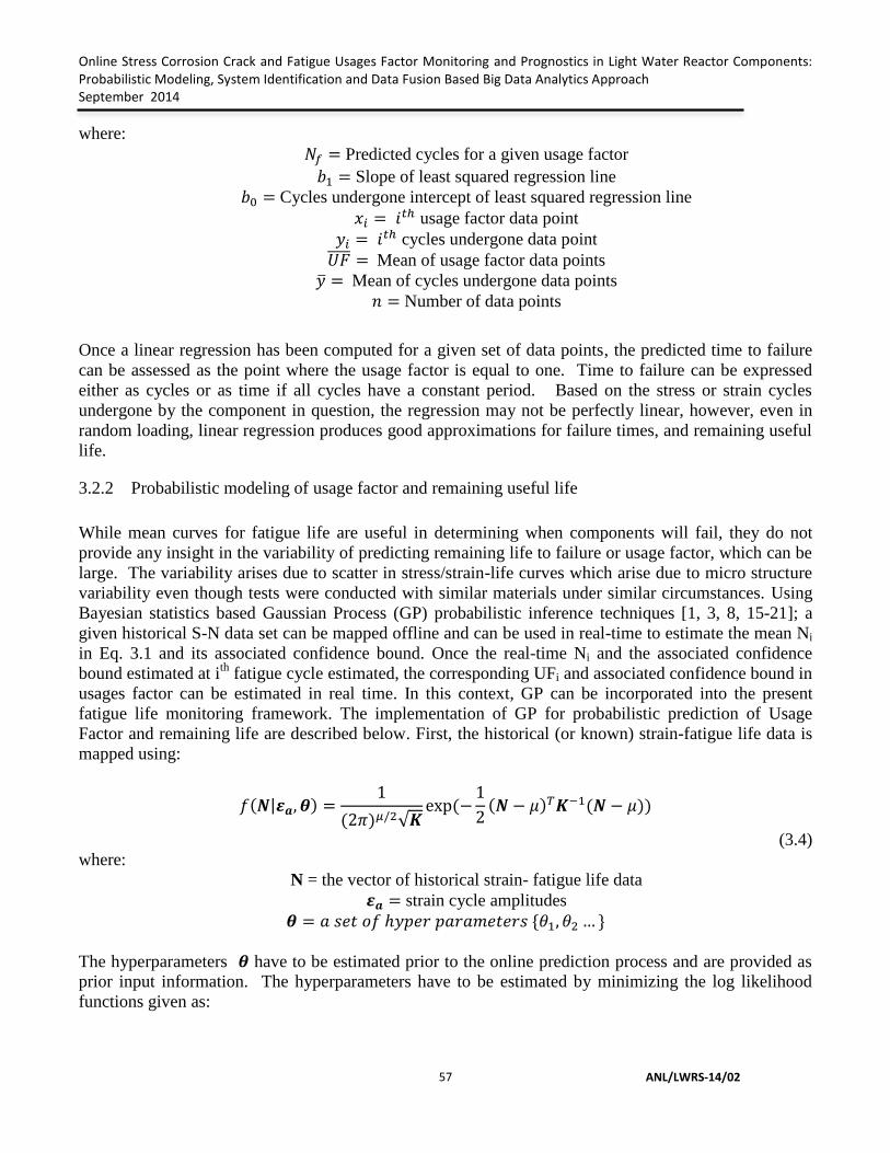
Online Stress Corrosion Crack and Fatigue Usages Factor Monitoring and Prognostics in Light Water Reactor Components: Probabilistic Modeling, System Identification and Data Fusion Based Big Data Analytics Approach September 2014
ANL/LWRS-14/02
57
where:
𝑁𝑓 = Predicted cycles for a given usage factor
𝑏1 = Slope of least squared regression line
𝑏0 = Cycles undergone intercept of least squared regression line
𝑥𝑖 = 𝑖𝑡ℎ usage factor data point
𝑦𝑖 = 𝑖𝑡ℎ cycles undergone data point
𝑈𝐹̅̅ ̅̅ = Mean of usage factor data points
�̅� = Mean of cycles undergone data points
𝑛 = Number of data points
Once a linear regression has been computed for a given set of data points, the predicted time to failure
can be assessed as the point where the usage factor is equal to one. Time to failure can be expressed
either as cycles or as time if all cycles have a constant period. Based on the stress or strain cycles
undergone by the component in question, the regression may not be perfectly linear, however, even in
random loading, linear regression produces good approximations for failure times, and remaining useful
life.
3.2.2 Probabilistic modeling of usage factor and remaining useful life
While mean curves for fatigue life are useful in determining when components will fail, they do not
provide any insight in the variability of predicting remaining life to failure or usage factor, which can be
large. The variability arises due to scatter in stress/strain-life curves which arise due to micro structure
variability even though tests were conducted with similar materials under similar circumstances. Using
Bayesian statistics based Gaussian Process (GP) probabilistic inference techniques [1, 3, 8, 15-21]; a
given historical S-N data set can be mapped offline and can be used in real-time to estimate the mean Ni
in Eq. 3.1 and its associated confidence bound. Once the real-time Ni and the associated confidence
bound estimated at ith
fatigue cycle estimated, the corresponding UFi and associated confidence bound in
usages factor can be estimated in real time. In this context, GP can be incorporated into the present
fatigue life monitoring framework. The implementation of GP for probabilistic prediction of Usage
Factor and remaining life are described below. First, the historical (or known) strain-fatigue life data is
mapped using:
𝑓(𝑵|𝜺𝒂, 𝜽) =1
(2𝜋)𝜇/2√𝑲exp(−
1
2(𝑵 − 𝜇)𝑇𝑲−1(𝑵 − 𝜇))
(3.4)
where:
N = the vector of historical strain- fatigue life data
𝜺𝒂 = strain cycle amplitudes
𝜽 = 𝑎 𝑠𝑒𝑡 𝑜𝑓 ℎ𝑦𝑝𝑒𝑟 𝑝𝑎𝑟𝑎𝑚𝑒𝑡𝑒𝑟𝑠 {𝜃1, 𝜃2 …}
The hyperparameters 𝜽 have to be estimated prior to the online prediction process and are provided as
prior input information. The hyperparameters have to be estimated by minimizing the log likelihood
functions given as:

Online Stress Corrosion Crack and Fatigue Usages Factor Monitoring and Prognostics in Light Water Reactor Components: Probabilistic Modeling, System Identification and Data Fusion Based Big Data Analytics Approach September 2014
ANL/LWRS-14/02 58
𝐿 = log (𝑓(𝜽|𝐻 = {휀𝑎, 𝑁𝑖}𝑖=1,2…𝑚)) = −1
2log (det (𝑲)) −
1
2𝐍𝑇𝐊−1𝐍 −
𝜇
2log (2𝜋)
(3.5)
Gaussian Processes can be used to model the entire historical (available) strain amplitude versus fatigue
life data 𝐻 = {휀𝑎, 𝑁𝑖}𝑖=1,2…𝑚 to a probabilistic input-output map as a black box model. Then the model
can be used to predict the output 𝑁𝑖 for a given input strain amplitude 휀𝑎 at a given instant of time or
fatigue cycle. In the above equations, K is the kernel matrix which is some sort of covariance matrix
which transfers the input-output data to a probabilistic high-dimensional space using a chosen kernel
function given as below [8]:
𝑘(휀𝑎𝑖, 휀𝑎𝑗
) = 휀𝑎𝑖
1
𝜃𝑙휀𝑎𝑗
+1
𝜃𝑙+ 𝜃𝑠
2
(3.6)
Where, 𝜃𝑙and 𝜃𝑠 are respectively the width and scatter hyperparameters. In Eq. 3.6 the first term
represents some sort of covariance relation between ith
and jth
strain amplitude, the second term map the
bias and third term maps the scatter in data, that could arises due to microstructural variability in
stress/strain~life data. Eq. 3.6 represents one of the simplest forms of kernel function and many
advanced form of the kernel function can be used for the purpose. A further evaluation of various kernel
functions is required, which is one of our future studies. The kernel matrix K can be estimated as:
𝑲(𝑖, 𝑗) = 𝑘(휀𝑎𝑖, 휀𝑎𝑗)𝑖=1,2…𝑚,𝑗=1,2…𝑚
(3.7)
Once the hyperparameters are estimated using the above equations and historical data, the mean life and
its variance of new strain amplitude (which would occur at any measured time) can be predicted in real
time using:
𝜇𝑁 = 𝒌𝑡𝑇𝑲𝑯
−𝟏𝑵𝑯
𝜎𝑁2 = 𝜅𝑡 − 𝑘𝑡
𝑇𝑲𝑯−𝟏𝑵𝑯
(3.8)
where:
KH= (m x m) historical kernel matrix
kt = (m x 1) vector
and κ is a scalar and can be found by partitioning the larger (m+1) x (m+1) kernel matrix as:
Kt = (𝑲𝑯 𝒌𝒕
𝒌𝒕𝑻 𝜿
)
(3.9)
with:
𝑘𝑡(𝑖, 𝑗)𝑖 = 1,2…𝑚,𝑗=𝑚+1 = 𝑘(휀𝑎𝑖, 휀𝑎𝑗)𝑖 = 1,2…𝑚,𝑗=𝑚+1
𝜅 = 𝐾(휀𝑎𝑖, 휀𝑎𝑗)𝑖 = 𝑚+1,𝑗=𝑚+1
Once the mean and variance are calculated at any given time, the mean life and 2σ (95.4 %) confidence
upper and lower limit of life corresponding to strain amplitude can be found as:
𝑁𝑚𝑒𝑎𝑛 = 𝜇𝑁
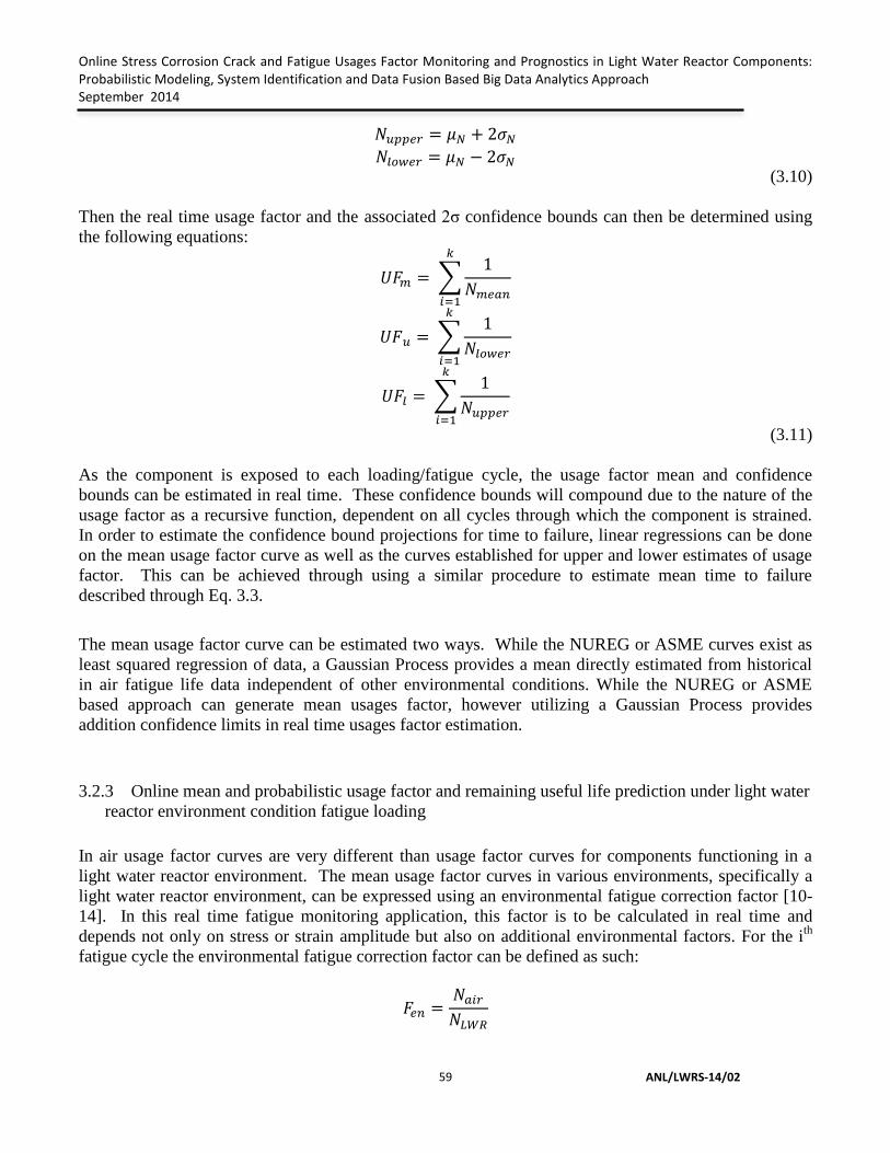
Online Stress Corrosion Crack and Fatigue Usages Factor Monitoring and Prognostics in Light Water Reactor Components: Probabilistic Modeling, System Identification and Data Fusion Based Big Data Analytics Approach September 2014
ANL/LWRS-14/02
59
𝑁𝑢𝑝𝑝𝑒𝑟 = 𝜇𝑁 + 2𝜎𝑁
𝑁𝑙𝑜𝑤𝑒𝑟 = 𝜇𝑁 − 2𝜎𝑁 (3.10)
Then the real time usage factor and the associated 2σ confidence bounds can then be determined using
the following equations:
𝑈𝐹𝑚 = ∑1
𝑁𝑚𝑒𝑎𝑛
𝑘
𝑖=1
𝑈𝐹𝑢 = ∑1
𝑁𝑙𝑜𝑤𝑒𝑟
𝑘
𝑖=1
𝑈𝐹𝑙 = ∑1
𝑁𝑢𝑝𝑝𝑒𝑟
𝑘
𝑖=1
(3.11)
As the component is exposed to each loading/fatigue cycle, the usage factor mean and confidence
bounds can be estimated in real time. These confidence bounds will compound due to the nature of the
usage factor as a recursive function, dependent on all cycles through which the component is strained.
In order to estimate the confidence bound projections for time to failure, linear regressions can be done
on the mean usage factor curve as well as the curves established for upper and lower estimates of usage
factor. This can be achieved through using a similar procedure to estimate mean time to failure
described through Eq. 3.3.
The mean usage factor curve can be estimated two ways. While the NUREG or ASME curves exist as
least squared regression of data, a Gaussian Process provides a mean directly estimated from historical
in air fatigue life data independent of other environmental conditions. While the NUREG or ASME
based approach can generate mean usages factor, however utilizing a Gaussian Process provides
addition confidence limits in real time usages factor estimation.
3.2.3 Online mean and probabilistic usage factor and remaining useful life prediction under light water
reactor environment condition fatigue loading
In air usage factor curves are very different than usage factor curves for components functioning in a
light water reactor environment. The mean usage factor curves in various environments, specifically a
light water reactor environment, can be expressed using an environmental fatigue correction factor [10-
14]. In this real time fatigue monitoring application, this factor is to be calculated in real time and
depends not only on stress or strain amplitude but also on additional environmental factors. For the ith
fatigue cycle the environmental fatigue correction factor can be defined as such:
𝐹𝑒𝑛 =𝑁𝑎𝑖𝑟
𝑁𝐿𝑊𝑅

Online Stress Corrosion Crack and Fatigue Usages Factor Monitoring and Prognostics in Light Water Reactor Components: Probabilistic Modeling, System Identification and Data Fusion Based Big Data Analytics Approach September 2014
ANL/LWRS-14/02 60
(3.12)
where:
𝐹𝑒𝑛𝑖= Environmental fatigue correction factor
𝑁𝑎𝑖𝑟 = Fatigue life in air
𝑁𝐿𝑊𝑅 = Fatigue life in light water reactor environment
This allows the environmental fatigue correction factor to be defined as follows with respect to usage
factor:
𝑈𝐹𝐿𝑊𝑅𝑖= ∑ 𝐹𝑒𝑛𝑘
∙ 𝑈𝑎𝑖𝑟𝑘
𝑖𝑘=1 (3.13)
where:
𝐹𝑒𝑛𝑘= Environmental fatigue correction factor
𝑈𝐹𝐿𝑊𝑅𝑖= Mean usage factor in a light water reactor environment
𝑈𝑎𝑖𝑟𝑖= Mean usage factor in an air environment for a single cycle
In Eq. 3.13, the mean environmental 𝑈𝐹𝐿𝑊𝑅𝑖 is to be estimated in real time for each i
th fatigue cycle
cumulatively. Whereas the in-air usages factors 𝑈𝑎𝑖𝑟𝑘 have to be estimated both using deterministic Eq.
3.1 and 3.2 or by using probabilistic mean usage factor 𝑈𝐹𝑚described by Eq. 3.4 through Eq. 3.11.
However the environmental field variable (e.g. temperature, water chemistry such as oxygen
concentration, etc.) dependent corrections factors 𝐹𝑒𝑛𝑘 have to be estimated in real time using the
equation provided in NUREG/CR-6909 [12]. For stainless steel the expression for mean environmental
fatigue correction factor is as follows:
ln(𝐹𝑒𝑛) = 0.734 − 𝑇′휀̇′𝑂′
𝑂′ = 0.281
휀̇′ = 0 (휀̇ > 0.4%/𝑠)
휀̇′ = ln (�̇�
0.4) (0.0004 ≤ 휀̇ ≤ 0.4%/𝑠)
휀̇′ = ln (0.0004
0.4) (휀̇ < 0.0004%/𝑠)
𝑇′ = 0 (𝑇 < 150°𝐶)
𝑇′ =𝑇−150
175 (150 ≤ 𝑇 < 325°𝐶)
𝑇′ = 1 (𝑇 ≥ 325°𝐶) (3.14)
𝑆 = Sulfur content in percent by weight
𝑇 = Temperature in degrees Celsius
𝐷𝑂 = Dissolved oxygen content in parts per million
휀̇ = Strain rate in percent per second

Online Stress Corrosion Crack and Fatigue Usages Factor Monitoring and Prognostics in Light Water Reactor Components: Probabilistic Modeling, System Identification and Data Fusion Based Big Data Analytics Approach September 2014
ANL/LWRS-14/02
61
The above mentioned equation is dependent on certain environmental factors: temperature, dissolved
oxygen level, and strain rate, and gives the mean environmental correction factor at any given fatigue
cycle and can be found for each stress cycle in real time. In calculating strain rate, average values
should be used to determine relevant parameters. However, when calculating temperature, the maximum
temperature for a given cycle should be used, as this provides the most conservative estimate. When
calculating remaining life, the same linear regression procedure should be used for light water reactor
environments as air environments.
These mean curves can be used as reference points for fatigue failure in PWR environments; however,
they do not give adequate scope for the variance for fatigue life in a PWR setting. In order to define this
variance, a similar GP based procedure described through Eq. 3.4 to 3.11 can be followed to model the
historical strain/stress versus life data for under PWR environment. Accordingly the upper bound of the
environmental usages factor, 𝑈𝐹𝑒𝑛 𝑢, and lower limit of the environmental usages factor, 𝑈𝐹𝑒𝑛 𝑙, can be
estimated using Eq. 3.11. To note that the NUREG equation includes the effects of environmental field
variables (e.g. temperature, water chemistry such as oxygen concentration, etc.) as independent variables
in addition to the strain/stress amplitude. However in the present GP model, the historical data 𝐻 ={휀𝑎, 𝑁𝑖}𝑖=1,2…𝑚 obtained through environmental fatigue tests are directly considered in the input-output
mapping. Hence, in this the strain is the only independent variable. However, the present GP model can
easily be augmented to multivariate mapping model with explicitly defining temperature, oxygen
concentration, etc. as additional independent variables. This is one of our future research interests.
In the present work, when referencing the historical data for GP based estimation of lower and upper
bound of the usages factor, the environmental fatigue correction factor need not be used. The historical
data references strain amplitudes in a pressurized water reactor environment, meaning that the effect of
the environment is already accounted for.
3.3 Numerical Results
3.3.1 High purity water and elevated temperature live fatigue test
Currently at Argonne National Laboratory different fatigue tests are being conducted under department
of energy (DOE)’s light water reactor sustainability program. The tests are being conducted for both
stainless steel grades (e.g. 316 SS) and low alloy steel (e.g 508) for both base metal and weld
(similar/dissimilar) specimens under either in-air room temperature or in-air elevated temperature or
under high purity water, elevated temperature or under PWR water, elevated temperature conditions
[22]. In the particular example discussed in this subsection, live fatigue monitoring (both live estimation
of fatigue usage factor and remaining life forecasting) was conducted on a 316 SS specimen undergoing
fatigue testing in a high purity water environment (with DO<5 ppb, Ph=6.4, conductivity <=0.1 uS/cm).
The water was maintained at 300 oC and under pressurized conditions similar in the case of a PWR type
rector. The specimen was inside a water tight autoclave and connected to the test frame load cell and
actuator through pull rods. Figure 3. 1 shows the environmental (in this case high purity water) test
frame and real time fatigue monitoring system. The fatigue monitoring system was developed based on a
National Instrument (NI) -PXI chassis with LABVIEW based codes for real-time data acquisition and

Online Stress Corrosion Crack and Fatigue Usages Factor Monitoring and Prognostics in Light Water Reactor Components: Probabilistic Modeling, System Identification and Data Fusion Based Big Data Analytics Approach September 2014
ANL/LWRS-14/02 62
MATLAB based codes for real time signal processing and live estimation of fatigue usages factor and
remaining useful life.
Figure 3. 1 ANL environmental test frame with live fatigue monitoring system.
During fatigue testing, frame stroke signals were collected intermittently through the above mentioned
fatigue monitoring system. Since the autoclave is watertight no extensometer could be used for
measurement of strain. Typically in a strain control fatigue test, specimen gauge area strains are
measured using an extensometer and used for controlling the test. Rather, in this case the crosshead
stroke displacement was measured through a Sapphire made displacement sensor and the measured
stroke displacement was used for controlling the fatigue test. However, for the purpose of fatigue usages
factor monitoring, the stroke measurement were converted to equivalent strain in real time using the
following stroke to strain mapping relation:
휀 = 𝑎0 + 𝑎1𝑑𝑠 + 𝑎2𝑑𝑠2 + 𝑎3𝑑𝑠
3 + 𝑎4𝑑𝑠4 + 𝑎5𝑑𝑠
5 + 𝑎6𝑑𝑠6 + 𝑎7𝑑𝑠
7 (3.15)

Online Stress Corrosion Crack and Fatigue Usages Factor Monitoring and Prognostics in Light Water Reactor Components: Probabilistic Modeling, System Identification and Data Fusion Based Big Data Analytics Approach September 2014
ANL/LWRS-14/02
63
Where, 휀 and 𝑑𝑠 are strain (%) and stroke (mm), respectively. Whereas the polynomial constants are
𝑎𝑖=0,1…7 = -0.0021055, 2.3843, -74.608, 1704, -12834, 46379, -81825, 56605. The above mapping
relation is based on in-air tensile test data earlier conducted at ANL, under similar temperature of 300 OC and for 316 SS specimen. To note that, in the present fatigue usages factor calculation (based on
strain versus life curve based approach) only peak equivalent strains are required and it is assumed that
the use of above tensile test based mapping relation can appropriately predict the equivalent peak strains
given the peak stroke measurements. In the in-air tensile test a high temperature extensometer was used
to measure the gage area strain of the specimen. It is assumed that in real nuclear power plants both
uniaxial and multiaxial rosette strain gauge can be mounted outside of the coolant system pipe or
pressure vessel to monitor the real time strain in the associated components. In the present test, load cell
signals were also collected intermittently to crosscheck the performance of the strain measurement based
fatigue monitoring algorithms. It is of note that, in real reactor it may not be always practical to equip
the reactor components with load cell and to monitor fatigue usages factor based on load cell (equivalent
stress) measurements. However, in the present case, similar to a stroke signal, the load cell
measurements can be converted to equivalent strain. For example in this case after converting load to
engineering stress, said engineering stress was converted to engineering strain using following
expression:
휀 = ε𝑝 + ε𝑒 =(𝜎−𝜎𝑦)
ℎ+
𝜎
𝐸
(3.16)
In Eq. 3.16 ε𝑒 and ε𝑝are the elastic and plastic strain component of total strain 휀, ℎ is the hardening
constant, 𝐸 is the elastic modulus and 𝜎𝑦is the yield stress, respectively. A preliminary linear isotropic
hardening approximation is assumed for estimating the hardening constant ℎ using a strain versus strain
curve. For example in this case the hardening constant ℎ = 244.26 𝑀𝑃𝑎 , 𝐸 = 157.212 𝐺𝑃𝑎 and
𝜎𝑦 = 156.067 were used to transform the stress to strain. The above parameters are estimated using the
stress-strain data obtained through an in-air 300 oC tensile test earlier conducted as part of the LWRS
program at ANL [refer T04 tensile test in reference 22]. Figure 3.2 shows the intermittently collected
stress history during the entire fatigue test of total 4373 cycles, while figure 3.3 show example of detail
stress path during 100-150 seconds. Similarly Figure 3.4 shows the intermittently estimated (from stroke
signal) strain history during the entire fatigue test of total 4373 cycles. During the fatigue test each
individual cycle load cell and stroke sensor measurements were recorded in a text file, from which the
peak and valley for load and stroke with respect to each cycle were determined. These were used to
determine the amplitude of each cycle strain either through stroke to strain mapping or through
load/stress to strain mapping discussed above. Once the cyclic strain amplitude estimated it was used to
estimate the corresponding strain rate to reach that strain amplitude. Once the cyclic strain rate was
estimated it was further used to estimate the cyclic environmental correction factor 𝐹𝑒𝑛𝑘 using Eq. 3.14.
Figure 3.5 shows the real time estimated environmental correction factor time history over the entire
4373 fatigue cycles. From the Figure 3.5 it can be seen that the 𝐹𝑒𝑛𝑘 time history remains flat over the
entire fatigue life, because the constant stroke control leads to constant strain amplitude. Use of nearly
constant strain amplitude leads to this nearly constant 𝐹𝑒𝑛𝑘 time history. However, in a real time
application with realistic arbitrary stress/strain transients the 𝐹𝑒𝑛𝑘 time history may not remain flat.
This is discussed in a later part of this section through a simulated example. In addition to 𝐹𝑒𝑛𝑘 at each
cycle ‘i’, the corresponding in-air usage factor was calculated using the Eq. 3.1 and 3.2. This

Online Stress Corrosion Crack and Fatigue Usages Factor Monitoring and Prognostics in Light Water Reactor Components: Probabilistic Modeling, System Identification and Data Fusion Based Big Data Analytics Approach September 2014
ANL/LWRS-14/02 64
information was then used to update the ith
cycle environmental usage factor 𝑈𝐹𝐿𝑊𝑅𝑖 as described
through Eq. 3.13. Figures 3.6 and 3.7 respectively show the stroke (or strain) and load (or stress)
measurements based real time estimated mean usages factor (blue line) using NUREG-6909 based
approach discussed above. From the figures it can be found that both stroke (or strain) and load (or
stress) based approach the mean usages factor prediction looks similar. This cross validates both the
approaches.
However, in the NUREG based approach discussed above, there is no confidence bound associated with
the mean prediction. The estimation of a probabilistic confidence bound is necessary for usages factor
estimation since micro structure variability related scatter in stress/strain- life curve can lead to large
variation in usage factor estimation either for offline calculation or in the present case of online
calculation. To address this issue, in the present work, the GP based approach discussed earlier was also
used to estimate the cyclic mean usages factor and the associated confidence bound. For the purpose,
once the strain cyclic strain amplitude is estimated in real time, the corresponding fatigue cycle 𝑁𝑖 is
found using Eq. 3.4. However in Eq. 3.4 the hyperparameters first must be estimated using the historical
stress/strain- life data (𝐻 = {휀𝑎, 𝑁𝑖}𝑖=1,2…𝑚) and through optimizing the log likelihood function given in
Eq. 3.5. These hyperparameters are fixed values and are used as input to the online estimation algorithm.
In the present work the strain amplitude versus fatigue life data for stainless steel under high temperature
water are used for estimating the hyperparameters. This data is taken from the Japan Nuclear Energy
Safety Organization report: JNES-SS-1005 [14]. These data corresponds to PWR water condition
fatigue test data and as shown in Figure 3.8. First these stress/strain-life data were converted by
logarithmic scaling. It is our assumption that scaling logarithmically will convert the original data to
scaled data which follows a normal distribution pattern, and then the Gaussian Process can be used for
mapping the stress/strain-life data (𝐻 = {휀𝑎, 𝑁𝑖}𝑖=1,2…𝑚). Figure 3.9 shows the histogram and
probability density function approximately at 0.6% strain amplitude for PWR water environment case.
This example figure confirms that the scaled stress/strain-life data approximately follows
Gaussian/Normal distribution. Note that, in the GP mapping all the data shown in Figure 3.8 were used
to form the GP model training data i.e. 𝐻 = {휀𝑎, 𝑁𝑖}𝑖=1,2…𝑚. For a given strain amplitude at a given
instant of time the GP model probabilistically interpolate the corresponding fatigue life. In addition, in
the present case of high purity water condition, it is assumed that the scatter effect due to microstructural
variability will be similar as in the case of PWR water condition.
For each cycle once the strain amplitude is estimated, the corresponding mean fatigue cycle 𝑁𝑖 and
associated 2σ (95.4%) confidence bounds were estimated using Eq. 3.10. Figure 3.10 shows the GP
estimated logarithmically scaled mean 𝑁𝑖 and associated 2σ confidence bound at different fatigue
cycles. From the figure it can be seen that mean 𝑁𝑖 and associated 2σ confidence bound remain fairly
constant although these are calculated in real time. This is because of the constant stroke (and hence
strain) amplitude fatigue test. This may not be the case for real life random loading case. Using these GP
estimated mean fatigue life and the associated 2σ confidence bounds, the ith
cycle mean usages factor
and the associated confidence bounds were updated in real time using Eq. 3.11. From the Figure 3.6 and
3.7 it can be seen the GP estimated mean usages factor and associated confidence bound based on
stroke/strain sensor measurements and load/stress sensor measurements. From the figures it can be seen
that the GP estimation yields fairly similar results for both stroke/strain and load/stress based approach.
In addition it can be seen that GP based mean usages factor history have similarity with the NUREG
based mean usage factor history. The mean curves may not exactly match each other because of the data

Online Stress Corrosion Crack and Fatigue Usages Factor Monitoring and Prognostics in Light Water Reactor Components: Probabilistic Modeling, System Identification and Data Fusion Based Big Data Analytics Approach September 2014
ANL/LWRS-14/02
65
set used in the both the cases and the extent of approximation used in both the cases. The purpose of the
present work is to demonstrate how in real time probabilistic usages factor can be calculated and
rigorous validation is beyond the scope of this exercise.
Similar to the usage factor, the remaining useful life (RUL) can be estimated in real time either using
above discussed NUREG based usage factor calculation or GP based usages factor calculation.
However, unlike the NUREG based approach the GP based approach can generate not only the mean
RUL but also the associated 95.4% confidence bound. As discussed earlier the RUL is calculated based
on linear approximation of real time estimated fatigue cycle versus usages factor data and using Eq. 3.3.
Figure 3.11 and 3.12 shows the time history of stroke/strain and load cell/stress sensor measurement
based RUL forecasting, respectively.
Figure 3. 2 Intermittent cyclic stress history for the high purity water fatigue test (F11).
0 2 4 6 8 10
x 104
-300
-200
-100
0
100
200
300
Total Time (s)
Str
ess
(MP
a)
Total Cycle Number = 4373

Online Stress Corrosion Crack and Fatigue Usages Factor Monitoring and Prognostics in Light Water Reactor Components: Probabilistic Modeling, System Identification and Data Fusion Based Big Data Analytics Approach September 2014
ANL/LWRS-14/02 66
Figure 3. 3 Magnified (between 100-150 seconds) stress history of F11 test.
Figure 3. 4 Intermittent transformed cyclic strain history for the high purity water fatigue test (F11)
using stroke-strain mapping.
100 105 110 115 120 125 130 135 140 145 150
-200
-150
-100
-50
0
50
100
150
200
Total Time (s)
Str
ess
(MP
a)
Total Cycle Number = 4373
0 2 4 6 8 10
x 104
-0.8
-0.6
-0.4
-0.2
0
0.2
0.4
0.6
Total Time (s)
Str
ain
(%
)
Total Cycle Number = 4373

Online Stress Corrosion Crack and Fatigue Usages Factor Monitoring and Prognostics in Light Water Reactor Components: Probabilistic Modeling, System Identification and Data Fusion Based Big Data Analytics Approach September 2014
ANL/LWRS-14/02
67
Figure 3. 5 Time history of environmental correction factor 𝐹𝑒𝑛𝑘
.
Figure 3. 6 Stroke sensor measurement based real time estimated usages factor time history for the high
purity water fatigue test (F11) using both NUREG-6909 based approach and GP based approach.
0 500 1000 1500 2000 2500 3000 3500 4000 45001
1.2
1.4
1.6
1.8
2
2.2
2.4
2.6
2.8
3
Cycles
En
vir
on
men
tal
Fati
gu
e C
orr
ecti
on
Fact
or
100
101
102
103
10-3
10-2
10-1
100
Usa
ge F
acto
r
Cycles
Based on stroke sensor measurement
Mean Usage Factor (NUREG/CR-6909)
Usage Factor Error Bounds (GP)
Mean Usage Factor (GP)
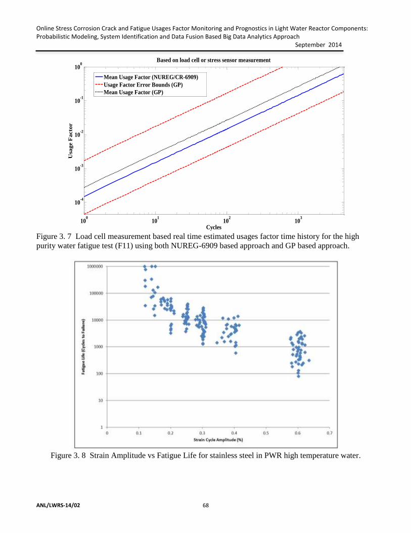
Online Stress Corrosion Crack and Fatigue Usages Factor Monitoring and Prognostics in Light Water Reactor Components: Probabilistic Modeling, System Identification and Data Fusion Based Big Data Analytics Approach September 2014
ANL/LWRS-14/02 68
Figure 3. 7 Load cell measurement based real time estimated usages factor time history for the high
purity water fatigue test (F11) using both NUREG-6909 based approach and GP based approach.
Figure 3. 8 Strain Amplitude vs Fatigue Life for stainless steel in PWR high temperature water.
100
101
102
103
10-4
10-3
10-2
10-1
100
Usa
ge F
acto
r
Cycles
Based on load cell or stress sensor measurement
Mean Usage Factor (NUREG/CR-6909)
Usage Factor Error Bounds (GP)
Mean Usage Factor (GP)
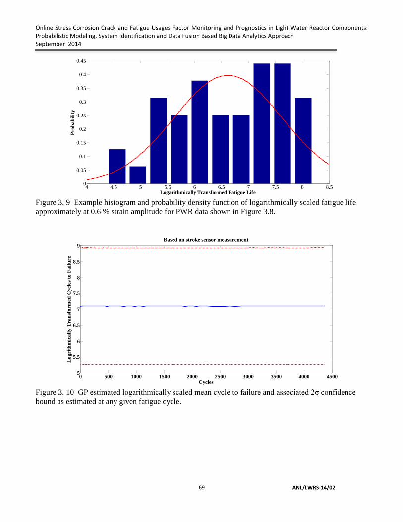
Online Stress Corrosion Crack and Fatigue Usages Factor Monitoring and Prognostics in Light Water Reactor Components: Probabilistic Modeling, System Identification and Data Fusion Based Big Data Analytics Approach September 2014
ANL/LWRS-14/02
69
Figure 3. 9 Example histogram and probability density function of logarithmically scaled fatigue life
approximately at 0.6 % strain amplitude for PWR data shown in Figure 3.8.
Figure 3. 10 GP estimated logarithmically scaled mean cycle to failure and associated 2σ confidence
bound as estimated at any given fatigue cycle.
4 4.5 5 5.5 6 6.5 7 7.5 8 8.50
0.05
0.1
0.15
0.2
0.25
0.3
0.35
0.4
0.45
Pro
ba
bil
ity
Logarithmically Transformed Fatigue Life
0 500 1000 1500 2000 2500 3000 3500 4000 45005
5.5
6
6.5
7
7.5
8
8.5
9
Cycles
Lo
gri
thm
ica
lly
Tra
nsf
orm
ed C
ycl
es t
o F
ail
ure
Based on stroke sensor measurement
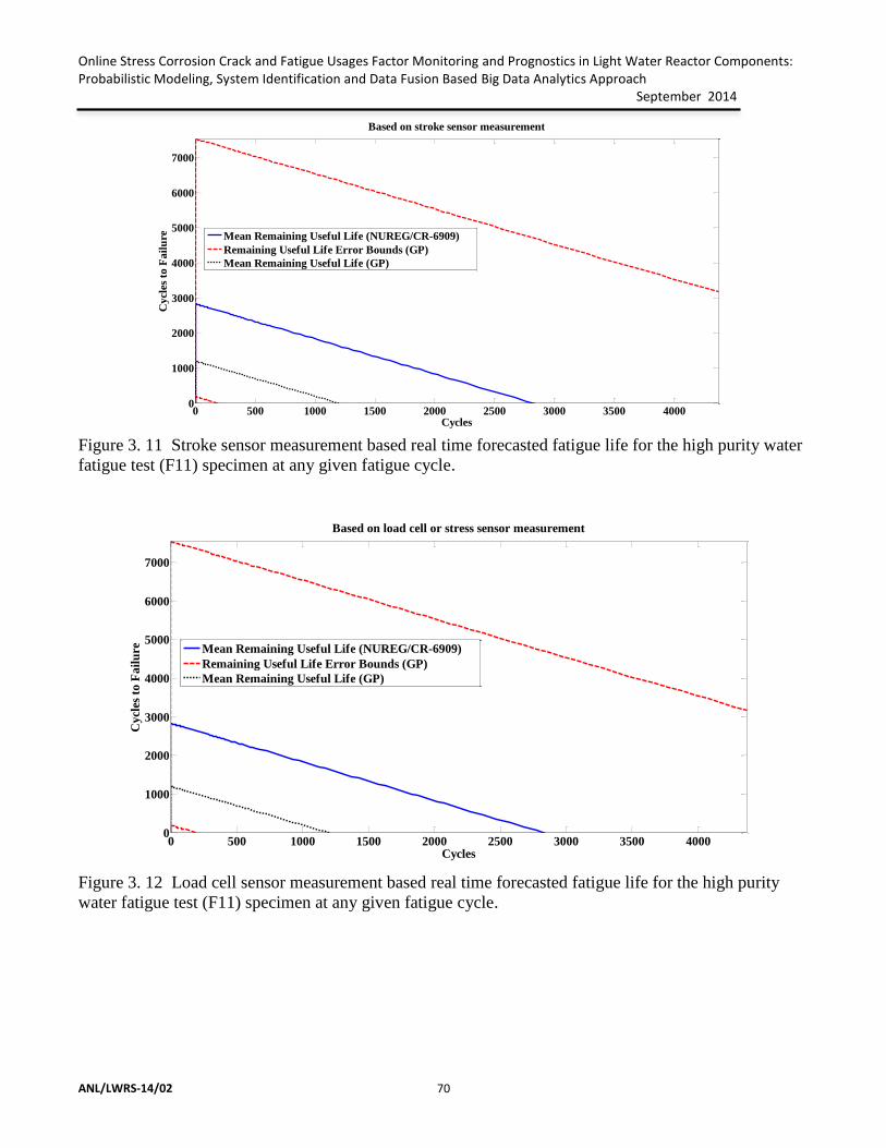
Online Stress Corrosion Crack and Fatigue Usages Factor Monitoring and Prognostics in Light Water Reactor Components: Probabilistic Modeling, System Identification and Data Fusion Based Big Data Analytics Approach September 2014
ANL/LWRS-14/02 70
Figure 3. 11 Stroke sensor measurement based real time forecasted fatigue life for the high purity water
fatigue test (F11) specimen at any given fatigue cycle.
Figure 3. 12 Load cell sensor measurement based real time forecasted fatigue life for the high purity
water fatigue test (F11) specimen at any given fatigue cycle.
0 500 1000 1500 2000 2500 3000 3500 40000
1000
2000
3000
4000
5000
6000
7000C
ycl
es t
o F
ail
ure
Cycles
Based on stroke sensor measurement
Mean Remaining Useful Life (NUREG/CR-6909)
Remaining Useful Life Error Bounds (GP)
Mean Remaining Useful Life (GP)
0 500 1000 1500 2000 2500 3000 3500 40000
1000
2000
3000
4000
5000
6000
7000
Cy
cles
to
Fa
ilu
re
Cycles
Based on load cell or stress sensor measurement
Mean Remaining Useful Life (NUREG/CR-6909)
Remaining Useful Life Error Bounds (GP)
Mean Remaining Useful Life (GP)

Online Stress Corrosion Crack and Fatigue Usages Factor Monitoring and Prognostics in Light Water Reactor Components: Probabilistic Modeling, System Identification and Data Fusion Based Big Data Analytics Approach September 2014
ANL/LWRS-14/02
71
3.3.2 PWR water and elevated temperature live fatigue test
A further test was run on a 316 stainless steel sample using water at 300° C with water chemistry more
reflective of a PWR environment. For the purpose the water chemistry was maintained with following
parameters: with gauge area target temperature of 300°C, water chemistry: 1000 ppm B as H3BO3, 2ppm
Li+ as LIOH, 20% H2/Bal N2 cover gas and DO < 5ppb, Ph 6.3, conductivity ≤ 23 uS/cm. The test was
run in the same set-up as the high purity water test previously discussed. Again, the same online
monitoring hardware-software system was employed to monitor fatigue usage factor and remaining
useful life for the test in real time. Again, stroke and load were collected, although only the data from
the stroke sensors (measuring equivalent strains) sensor are discussed here, as that would more than
likely be the setup in a real nuclear reactor, where strain can easily be measured. The test was cut short
after 499 cycles as an anomaly was discovered in the testing setup. Text files were again collected
intermittently for each cycle, from which peak and valleys for stroke were determined. As with the
previous test, the intermittently collected stroke was converted to strain using equation 3.15. This
intermittent strain history is show in figure 3.13. Again, using the same methodology as in the previous
test, strain rate was calculated from the strain amplitudes and used, in conjunction with temperature and
dissolved oxygen content, to determine an environmental fatigue correction factor (𝐹𝑒𝑛𝑖). Figure 3.14
shows these results for each cycle calculated in real time for all 499 cycles. It can be noted that the time
history remains flat, again due to the constant strain amplitude causing a constant strain rate.
Temperature and dissolved oxygen content were also kept constant throughout the test.
The mean in-air fatigue life was found to determine an in-air mean usage factor by using Eq. 3.1 and
3.2. This was used in conjunction with the 𝐹𝑒𝑛𝑘 to determine a mean fatigue life and usage factor
according to the NUREG method. This method is appropriate; however it lacks a scope to include the
effect of large scatter in fatigue life. To alleviate these issues again, the GP based approach discussed
above was used to determine bounds for fatigue life and thereby usage factor based on historical PWR
strain amplitude- fatigue life data. This uses the same process (Eq. 3.4-3.11) as the previous test. This
process is assumed valid as the normal distribution is followed by the data used here, which is the same
data used in the previous test. Figure 3.15 shows the real time estimated mean and corresponding error
bounds for (taken from the GP) for logarithmically transformed fatigue life. Much like figure 3.14,
these values are flat due to the constant strain cycles. Figure 3.16 shows the correspondingly estimated
usage factor time histories. Again, we see that both the GP and NUREG based usages factor fall well
within the GP estimated confidence bounds, again validating both methods, while also providing
valuable confidence interval data to account for scatter resulting from microstructure variability. Again,
a linear regression was employed for determination of remaining useful life. The time history for
remaining useful life is shown in figure 3.17.
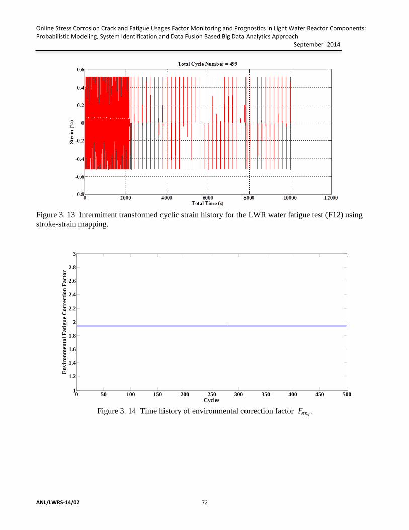
Online Stress Corrosion Crack and Fatigue Usages Factor Monitoring and Prognostics in Light Water Reactor Components: Probabilistic Modeling, System Identification and Data Fusion Based Big Data Analytics Approach September 2014
ANL/LWRS-14/02 72
Figure 3. 13 Intermittent transformed cyclic strain history for the LWR water fatigue test (F12) using
stroke-strain mapping.
Figure 3. 14 Time history of environmental correction factor 𝐹𝑒𝑛𝑖
.
0 50 100 150 200 250 300 350 400 450 5001
1.2
1.4
1.6
1.8
2
2.2
2.4
2.6
2.8
3
Cycles
En
vir
on
men
tal
Fa
tig
ue
Co
rrec
tio
n F
act
or

Online Stress Corrosion Crack and Fatigue Usages Factor Monitoring and Prognostics in Light Water Reactor Components: Probabilistic Modeling, System Identification and Data Fusion Based Big Data Analytics Approach September 2014
ANL/LWRS-14/02
73
Figure 3. 15 GP estimated logarithmically scaled mean cycle to failure and associated 2σ confidence
bound as estimated at any given fatigue cycle.
Figure 3. 16 Stroke sensor measurement based real time estimated usage factor time history for the
PWR water fatigue test (F12) using both NUREG-6909 based approach and GP based approach.

Online Stress Corrosion Crack and Fatigue Usages Factor Monitoring and Prognostics in Light Water Reactor Components: Probabilistic Modeling, System Identification and Data Fusion Based Big Data Analytics Approach September 2014
ANL/LWRS-14/02 74
Figure 3. 17 Strain gage sensor measurement based real time forecasted fatigue life for the PWR water
fatigue test (F12) specimen at any given fatigue cycle.
3.3.3 In-air and room temperature live fatigue test
A further test was run on a 316 stainless steel sample in a room temperature air environment. The test
was run in an in-air set up, which provided added advantage of directly measuring the spacemen gage
area strain using an extensometer. The test was conducted under room temperature condition. Compared
to the previous two discussed test cases there was no need for a stroke to strain conversion. Text files
were again collected continuously for each cycle, from which peak and valleys for strain were
determined. Unlike the previous two cases in the present case, the data were collected continuously for
each individual cycle. The test was run to failure, which occurred at 9096 cycles. Again here, imagining
a similar real reactor condition where strain can easily be monitored, in the present discussed case, only
strain data was used in estimation of usage factor and remaining useful life. This strain history is show
in figure 3.18.
The mean in-air fatigue life was found to determine an in-air mean usage factor by using equations 1 and
2. This was used to determine a mean fatigue life and usage factor according to the NUREG method.
Again, the GP based approach was used to determine bounds for fatigue life and thereby usage factor
based on historical in-air strain amplitude- fatigue life data. This uses the same process (Equations 3.4-
3.11) as the previous test. This process utilized in- air strain amplitude- fatigue life data from the JNES
report: JNES-SS-1005 [14] and the taken strain-life data is shown in Figure 3.19. The same Gaussian
Process was run on this set of data; however in-air historical data was used instead. Figure 3.19 shows
data used to model the scatter, while figure 3.20 shows the example histogram and corresponding
probability distribution function for .2% strain. This figure confirms that the scaled data approximately
0 50 100 150 200 250 300 350 400 4500
1000
2000
3000
4000
5000
6000
7000
Cy
cles
to
Fa
ilu
re
Cycles
Remaining Useful Life for Strain Data
Mean Remaining Useful Life (NUREG/CR-6909)
Remaining Useful Life Error Bounds (GP)
Mean Remaining Useful Life (GP)

Online Stress Corrosion Crack and Fatigue Usages Factor Monitoring and Prognostics in Light Water Reactor Components: Probabilistic Modeling, System Identification and Data Fusion Based Big Data Analytics Approach September 2014
ANL/LWRS-14/02
75
follows a Gaussian or Normal Distribution. Again, a similar process was used to determine a mean and
error bounds for fatigue life. Figure 3.21 shows the real time estimated mean and corresponding error
bounds for (taken from the GP) for logarithmically transformed fatigue life. Much like figures 3.10 and
3.15, these values are flat due to the constant strain cycles. The fatigue life values were used to
determine real time usage factor. Figure 3.22 shows these results of usage factor plotting by using both
GP and NUREG based approaches. Again, we see that the NUREG and GP based approach estimate
similar mean usages factor history, again validating the GP based methods, while also providing
valuable confidence bounds to account for scatter resulting from microstructure variability. Again, a
linear regression was employed for determination of remaining useful life. The time history for
remaining useful life is shown in figure 3.23.
Figure 3. 18 Cyclic strain history for the in air fatigue test (F09).

Online Stress Corrosion Crack and Fatigue Usages Factor Monitoring and Prognostics in Light Water Reactor Components: Probabilistic Modeling, System Identification and Data Fusion Based Big Data Analytics Approach September 2014
ANL/LWRS-14/02 76
Figure 3. 19 Strain amplitude vs in-air test fatigue life for stainless steel .
Figure 3. 20 Example histogram and probability density function of logarithmically scaled fatigue life
approximately at 0.2% strain amplitude for in-air condition data shown in Figure 3.19.
1
10
100
1000
10000
100000
1000000
0 0.5 1 1.5
Ftig
ue
Lif
e (
Cyc
les
to F
ailu
re)
Strain Amplitude (%)
10.5 11 11.5 12 12.5 13 13.5 140
0.1
0.2
0.3
0.4
0.5
0.6
0.7
Pro
bab
ilit
y
Logarithmically Transformed Fatigue Life

Online Stress Corrosion Crack and Fatigue Usages Factor Monitoring and Prognostics in Light Water Reactor Components: Probabilistic Modeling, System Identification and Data Fusion Based Big Data Analytics Approach September 2014
ANL/LWRS-14/02
77
Figure 3. 21 Strain gage sensor measurement based real time forecasted fatigue life for the in air fatigue
test (F09) specimen at any given fatigue cycle.
Figure 3. 22 Strain gage measurement based real time estimated usage factor time history for the in air
fatigue test (F09) using both NUREG-6909 based approach and GP based approach.
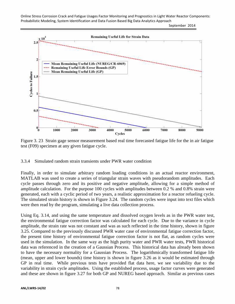
Online Stress Corrosion Crack and Fatigue Usages Factor Monitoring and Prognostics in Light Water Reactor Components: Probabilistic Modeling, System Identification and Data Fusion Based Big Data Analytics Approach September 2014
ANL/LWRS-14/02 78
Figure 3. 23 Strain gage sensor measurement based real time forecasted fatigue life for the in air fatigue
test (F09) specimen at any given fatigue cycle.
3.3.4 Simulated random strain transients under PWR water condition
Finally, in order to simulate arbitrary random loading conditions in an actual reactor environment,
MATLAB was used to create a series of triangular strain waves with pseudorandom amplitudes. Each
cycle passes through zero and its positive and negative amplitude, allowing for a simple method of
amplitude calculation. For the purpose 100 cycles with amplitudes between 0.2 % and 0.8% strain were
generated, each with a cyclic period of two years, a realistic approximation for a reactor refueling cycle.
The simulated strain history is shown in Figure 3.24. The random cycles were input into text files which
were then read by the program, simulating a live data collection process.
Using Eq. 3.14, and using the same temperature and dissolved oxygen levels as in the PWR water test,
the environmental fatigue correction factor was calculated for each cycle. Due to the variance in cycle
amplitude, the strain rate was not constant and was as such reflected in the time history, shown in figure
3.25. Compared to the previously discussed PWR water case of environmental fatigue correction factor,
the present time history of environmental fatigue correction factor is not flat, as random cycles were
used in the simulation. In the same way as the high purity water and PWR water tests, PWR historical
data was referenced in the creation of a Gaussian Process. This historical data has already been shown
to have the necessary normality for a Gaussian Process. The logarithmically transformed fatigue life
(mean, upper and lower bounds) time history is shown in figure 3.26 as it would be estimated through
GP in real time. While previous tests have provided flat data here, we see variability due to the
variability in strain cycle amplitudes. Using the established process, usage factor curves were generated
and these are shown in figure 3.27 for both GP and NUREG based approach. Similar as previous cases

Online Stress Corrosion Crack and Fatigue Usages Factor Monitoring and Prognostics in Light Water Reactor Components: Probabilistic Modeling, System Identification and Data Fusion Based Big Data Analytics Approach September 2014
ANL/LWRS-14/02
79
the GP based approach not only estimated the mean usages factor but also the associated confidence
bound for the discussed strain time history. This shows the microstructural variability associated scatter
can be incorporated in the usages factor results. In addition, we can still use a linear regression to
determine remaining useful life, and this has been employed with the results shown in figure 3.28. Due
to the large oscillations, the first 10-20 cycles do not accurately reflect remaining useful life; however a
general downward trend can be noted in all of the curves with shapes similar to results in earlier sections
of this report. The downward trend may be difficult to see, due to poor scaling on the original graph, so
a zoomed in error bound reflecting the true downward trending behavior is provided in figure 3.29 that
shows the lower bound in Figure 3.28.
Figure 3. 24 Pseudorandom cyclic strain history.
0 20 40 60 80 100 120 140 160 180 200-0.8
-0.6
-0.4
-0.2
0
0.2
0.4
0.6
0.8
Str
ain
Time(Yr.)

Online Stress Corrosion Crack and Fatigue Usages Factor Monitoring and Prognostics in Light Water Reactor Components: Probabilistic Modeling, System Identification and Data Fusion Based Big Data Analytics Approach September 2014
ANL/LWRS-14/02 80
Figure 3. 25 Time history of environmental correction factor 𝐹𝑒𝑛𝑖
.
Figure 3. 26 Predicted logarithmically transformed time history of fatigue life (mean, upper and lower
bounds), as it would be estimated through GP in a realistic reactor condition.

Online Stress Corrosion Crack and Fatigue Usages Factor Monitoring and Prognostics in Light Water Reactor Components: Probabilistic Modeling, System Identification and Data Fusion Based Big Data Analytics Approach September 2014
ANL/LWRS-14/02
81
Figure 3. 27 Estimated usage factor time history for pseudorandom cycles using both NUREG-6909
based approach and GP based approach.
Figure 3. 28 Forecasted time history of fatigue life for random cycles.

Online Stress Corrosion Crack and Fatigue Usages Factor Monitoring and Prognostics in Light Water Reactor Components: Probabilistic Modeling, System Identification and Data Fusion Based Big Data Analytics Approach September 2014
ANL/LWRS-14/02 82
Figure 3. 29 Magnified Figure 3.28 showing clear decreasing trend of cycles to failure (zoomed to show
lower bound in Figure 3.28).
3.4 Conclusions
Online fatigue monitoring and life forecasting tools can be used to accurately monitor fatigue damage in
real time, that can reduces risk in operating nuclear reactors and allows for more current, accurate
knowledge of remaining useful life. In the present work a Gaussian Process based probabilistic and
NUREG based deterministic framework is discussed to estimate both the time to failure and usage factor
in real time. This approach will help for more accurate component life monitoring in real time and
hence will help in efficient management of nuclear reactor component life cycles improving both safety
and economic benefits.
The proposed framework validated against simplified laboratory scale live tests and using simulated
complex transients. The presented research results are based on our preliminary efforts on real time and
probabilistic fatigue monitoring of nuclear reactor components, and need advanced validation.

Online Stress Corrosion Crack and Fatigue Usages Factor Monitoring and Prognostics in Light Water Reactor Components: Probabilistic Modeling, System Identification and Data Fusion Based Big Data Analytics Approach September 2014
ANL/LWRS-14/02
83
References
1. Mohanty, S., Structural Health Monitoring and Condition Based Fatigue Damage Prognosis of
Complex Metallic Structures, PhD Thesis, Arizona State University, Tempe, Arizona, 2010.
2. Mohanty S., Chattopadhyay A., Wei J., Peralta P., Unsupervised time-series fatigue damage state
estimation of complex structure using ultrasound based narrowband and broadband active
sensing. Journal of Structural Durability and Health Monitoring, 2009, 5(3):227-250.
3. Mohanty, S, Chattopadhyay, A., and Peralta, P., "Adaptive residual useful life estimation of a
structural hotspot." Journal of Intelligent Material Systems and Structures, 2010, 21(3): 321-335.
4. Bakhtiari S., Mohanty S., Prokofiev I., Tregoning R., Condition based prognostics of passive
components – a new era for nuclear power plant life management, International Atomic Energy
Agency conference, 2012, IAEA-CN-194-097.
5. International Atomic Energy Agency, Advanced surveillance, diagnostic and prognostic
techniques in monitoring structures, systems and components in nuclear power plants. IAEA
Nuclear Energy Series, 2013, NP-T-3.14.
6. http://www.ne.anl.gov/facilities/eda/steamgen.html
7. Ljung L, System Identification Toolbox. The Mathworks, Inc., Massachusetts, 1995.
8. Rasmussen C., Williams C., Gaussian Processes for Machine Learning. MIT Press,
Massachusetts, 2006.
9. Musallam, M., and Johnson., C. M., “An Efficient Implementation of the Rainflow Counting
Algorithm for Life Consumption Estimation,” IEEE Transactions on Reliability, 2012, 61(4):
978-986.
10. Carney, C. and Gillman. T., “Stress-Based Fatigue Monitoring: Methodology for Fatigue
Monitoring of Class 1 Nuclear Components in a Reactor Water Environment,” Electric Power
Research Institute, 2011.
11. Chopra, O. K. and Shack, W. J., “Review of the Margins for ASME Code Fatigue Design
Curve-Effects of Surface Roughness and Material Variability,” Report, Argonne National
Laboratory, September 2003, NUREG/CR-6815.
12. O. Chopra and G. L. Stevens. “Effect of LWR Coolant Environments on the Fatigue Life of
Reactor Materials,” United States Regulatory Commission, 2014, NUREG/CR-6909.
13. Guidelines for Evaluating Fatigue Analysis Incorporating the Life Reduction of Metal
Components Due to the Effects of the Light-Water Reactor Environment for New Reactors,
United States Nuclear Regulatory Commission, 2007, Guide 1.207.
Online Stress Corrosion Crack and Fatigue Usages Factor Monitoring and Prognostics in Light Water Reactor Components: Probabilistic Modeling, System Identification and Data Fusion Based Big Data Analytics Approach September 2014
ANL/LWRS-14/02 84
14. Environmental Fatigue Evaluation Method for Nuclear Power Plants, Japan Nuclear Energy
Safety Organization, March 2011, Report no. JNES-SS-1005.
15. Snelson, E., “Flexible and Efficient Gaussian Process Models for Machine Learning,” Ph.D.
Thesis, University of London, 2007.
16. Lawrence, N “Probabilistic Non-Linear Principal Component Analysis with Gaussian Process
Latent Variable Models,” Journal of Machine Learning Research, 2005, 6: 1783-1816.
17. Mohanty, S.., Das, S., Chattopadhyay, A., and Peralta, P., “Gaussian Process Time Series Model
for Life Prognosis of Metallic Structure”, Journal of Intelligent Material Systems and Structures,
2008, 20(8):887-896.
18. Mohanty, S., Chattopadhyay, A., Wei, J and Peralta, P., “Real time Damage State Estimation and
Condition Based Residual Useful Life Estimation of a Metallic Specimen under Biaxial
Loading”, Structural Durability & Health Monitoring Journal, 2009, 5(1): 33-55.
19. Mohanty, S., Chattopadhyay, A., Peralta, P., and Das, S., “Off-Line and On-Line Fatigue Crack
Growth Prediction Using Multivariate Gaussian Process, Journal of Experimental Mechanics,
2009
20. Chattopadhyay, A., and Mohanty, S., “Gaussian Process Damage Prognosis under Random and
Flight Profile Fatigue Loading,” Machine Learning and Knowledge Discovery for Engineering
Systems Health Management, CRC Press, 2012.
21. Mohanty, S., Chattopadhyay, A., and Rajadas, John N. “Bayesian Nonlinear Model for Dynamic
Strain Mapping and Real-time Damage State Estimation under Biaxial Random Fatigue
Loading”, AIAA Journal, 2012, 50 (4): 769-777.
22. Mohanty, S., Soppet, W. K., Majumdar, S. and Natesan, K. “Report on Assessment of
Environmentally-Assisted Fatigue for LWR Extended Service Conditions”, March 2013,
ANL/LWRS-13/3.

Online Stress Corrosion Crack and Fatigue Usages Factor Monitoring and Prognostics in Light Water Reactor Components: Probabilistic Modeling, System Identification and Data Fusion Based Big Data Analytics Approach September 2014
1
This page intentionally left blank


Argonne National Laboratory is a U.S. Department of Energy laboratory managed by UChicago Argonne, LLC
Nuclear Engineering Division Argonne National Laboratory
9700 South Cass Avenue, Bldg. 208
Argonne, IL 60439
www.anl.gov