online passive-aggressive algorithms - technion...
TRANSCRIPT
Journal of Machine Learning Research 7 (2006) 551–585 Submitted 5/05; Published 3/06
Online Passive-Aggressive Algorithms
Koby Crammer∗ [email protected]
Ofer Dekel [email protected] Keshet [email protected] Shalev-Shwartz [email protected] Singer† [email protected] of Computer Science and EngineeringThe Hebrew UniversityJerusalem, 91904, Israel
Editor: Manfred K. Warmuth
AbstractWe present a family of margin based online learning algorithms for various prediction tasks. In
particular we derive and analyze algorithms for binary and multiclass categorization, regression,uniclass prediction and sequence prediction. The update steps of our different algorithms are allbased on analytical solutions to simple constrained optimization problems. This unified view al-lows us to prove worst-case loss bounds for the different algorithms and for the various decisionproblems based on a single lemma. Our bounds on the cumulative loss of the algorithms are relativeto the smallest loss that can be attained by any fixed hypothesis, and as such are applicable to bothrealizable and unrealizable settings. We demonstrate someof the merits of the proposed algorithmsin a series of experiments with synthetic and real data sets.
1. Introduction
In this paper we describe and analyze several online learning tasks through the same algorithmicprism. We first introduce a simple online algorithm which we call Passive-Aggressive (PA) for on-line binary classification (see also (Herbster, 2001)). We then proposetwo alternative modificationsto the PA algorithm which improve the algorithm’s ability to cope with noise. We provide a unifiedanalysis for the three variants. Building on this unified view, we show how to generalize the binarysetting to various learning tasks, ranging from regression to sequence prediction.
The setting we focus on is that of online learning. In the online setting, a learning algorithm ob-serves instances in a sequential manner. After each observation, the algorithm predicts an outcome.This outcome can be as simple as a yes/no (+/−) decision, as in the case of binary classificationproblems, and as complex as a string over a large alphabet. Once the algorithm has made a predic-tion, it receives feedback indicating the correct outcome. Then, the online algorithm may modifyits prediction mechanism, presumably improving the chances of making an accurate prediction onsubsequent rounds. Online algorithms are typically simple to implement and their analysis oftenprovides tight bounds on their performance (see for instance Kivinen and Warmuth (1997)).
∗. Current affiliation: Department of Computer and Information Science, University of Pennsylvania, 3330 WalnutStreet, Philadelphia, PA 19104, USA.
†. Current affiliation: Google, Moutain View, CA 94043, USA.
c©2006 Koby Crammer, Ofer Dekel, Joseph Keshet, Shai Shalev-Shwartz and Yoram Singer.
CRAMMER, DEKEL, KESHET, SHALEV-SHWARTZ AND SINGER
Our learning algorithms use hypotheses from the set of linear predictors.While this class mayseem restrictive, the pioneering work of Vapnik (1998) and colleaguesdemonstrates that by us-ing Mercer kernels one can employ highly non-linear predictors and still entertain all the formalproperties and simplicity of linear predictors. For concreteness, our presentation and analysis areconfined to the linear case which is often referred to as the primal version (Vapnik, 1998; Cristianiniand Shawe-Taylor, 2000; Scholkopf and Smola, 2002). As in other constructions of linear kernelmachines, our paradigm also builds on the notion of margin.
Binary classification is the first setting we discuss in the paper. In this setting each instanceis represented by a vector and the prediction mechanism is based on a hyperplane which dividesthe instance space into two half-spaces. The margin of an example is proportional to the distancebetween the instance and the hyperplane. The PA algorithm utilizes the margin tomodify the currentclassifier. The update of the classifier is performed by solving a constrained optimization problem:we would like the new classifier to remain as close as possible to the current one while achievingat least a unit margin on the most recent example. Forcing a unit margin might turn out to be tooaggressive in the presence of noise. Therefore, we also describe two versions of our algorithm whichcast a tradeoff between the desired margin and the proximity to the current classifier.
The above formalism is motivated by the work of Warmuth and colleagues for deriving onlinealgorithms (see for instance (Kivinen and Warmuth, 1997) and the references therein). Furthermore,an analogous optimization problem arises in support vector machines (SVM)for classification (Vap-nik, 1998). Indeed, the core of our construction can be viewed as finding a support vector machinebased on a single example while replacing the norm constraint of SVM with a proximity constraintto the current classifier. The benefit of this approach is two fold. First, we get a closed form solutionfor the next classifier. Second, we are able to provide a unified analysisof the cumulative loss forvarious online algorithms used to solve different decision problems. Specifically, we derive andanalyze versions for regression problems, uniclass prediction, multiclassproblems, and sequenceprediction tasks.
Our analysis is in the realm of relative loss bounds. In this framework, the cumulative losssuffered by an online algorithm is compared to the loss suffered by a fixedhypothesis that may bechosen in hindsight. Our proof techniques are surprisingly simple and the proofs are fairly shortand easy to follow. We build on numerous previous results and views. The mere idea of deriving anupdate as a result of a constrained optimization problem compromising of two opposing terms, hasbeen largely advocated by Littlestone, Warmuth, Kivinen and colleagues (Littlestone, 1989; Kivi-nen and Warmuth, 1997). Online margin-based prediction algorithms are alsoquite prevalent. Theroots of many of the papers date back to the Perceptron algorithm (Agmon, 1954; Rosenblatt, 1958;Novikoff, 1962). More modern examples include the ROMMA algorithm of Liand Long (2002),Gentile’s ALMA algorithm (Gentile, 2001), the MIRA algorithm (Crammer and Singer, 2003b), andthe NORMA algorithm (Kivinen et al., 2002). The MIRA algorithm is closely related to the workpresented in this paper, and specifically, the MIRA algorithm for binary classification is identical toour basic PA algorithm. However, MIRA was designed forseparablebinary and multiclass prob-lems whereas our algorithms also apply to nonseparable problems. Furthermore, the loss boundsderived in Crammer and Singer (2003b) are inferior and less general than the bounds derived in thispaper. The NORMA algorithm also shares a similar view of classification problems. Rather thanprojecting the current hypothesis onto the set of constraints induced by the most recent example,NORMA’s update rule is based on a stochastic gradient approach (Kivinen et al., 2002). Of all thework on online learning algorithms, the work by Herbster (2001) is probably the closest to the work
552

ONLINE PASSIVE-AGGRESSIVEALGORITHMS
presented here. Herbster describes and analyzes a projection algorithm that, like MIRA, is essen-tially the same as the basic PA algorithm for the separable case. We surpass MIRA and Herbster’salgorithm by providing bounds for both the separable and the nonseparable settings using a unifiedanalysis. As mentioned above we also extend the algorithmic framework and theanalysis to morecomplex decision problems.
The paper is organized as follows. In Sec. 2 we formally introduce the binary classificationproblem and in the next section we derive three variants of an online learning algorithm for thissetting. The three variants of our algorithm are then analyzed in Sec. 4. Wenext show how tomodify these algorithms to solve regression problems (Sec. 5) and uniclass prediction problems(Sec. 6). We then shift gears to discuss and analyze more complex decision problems. Specifically,in Sec. 7 we describe a generalization of the algorithms to multiclass problems andfurther extendthe algorithms to cope with sequence prediction problems (Sec. 9). We describe experimental resultswith binary and multiclass problems in Sec. 10 and conclude with a discussion offuture directionsin Sec. 11.
2. Problem Setting
As mentioned above, the paper describes and analyzes several online learning tasks through thesame algorithmic prism. We begin with binary classification which serves as the mainbuilding blockfor the remainder of the paper. Online binary classification takes place in a sequence of rounds. Oneach round the algorithm observes an instance and predicts its label to be either+1 or−1. After theprediction is made, the true label is revealed and the algorithm suffers aninstantaneous losswhichreflects the degree to which its prediction was wrong. At the end of each round, the algorithm usesthe newly obtained instance-label pair to improve its prediction rule for the rounds to come.
We denote the instance presented to the algorithm on roundt by xt , and for concreteness weassume that it is a vector inRn. We assume thatxt is associated with a unique labelyt ∈ {+1,−1}.We refer to each instance-label pair(xt ,yt) as anexample. The algorithms discussed in this papermake predictions using a classification function which they maintain in their internal memory andupdate from round to round. We restrict our discussion to classification functions based on a vectorof weightsw ∈ R
n, which take the form sign(w · x). The magnitude|w · x| is interpreted as thedegree of confidence in this prediction. The task of the algorithm is therefore to incrementally learnthe weight vectorw. We denote bywt the weight vector used by the algorithm on roundt, and referto the termyt(wt ·xt) as the (signed)marginattained on roundt. Whenever the margin is a positivenumber then sign(wt ·xt) = yt and the algorithm has made a correct prediction. However, we are notsatisfied by a positive margin value and would additionally like the algorithm to predict with highconfidence. Therefore, the algorithm’s goal is to achieve a margin of at least 1 as often as possible.On rounds where the algorithm attains a margin less than 1 it suffers an instantaneous loss. Thisloss is defined by the followinghinge-lossfunction,
ℓ(
w;(x,y))
=
{
0 y(w ·x) ≥ 11−y(w ·x) otherwise
. (1)
Whenever the margin exceeds 1, the loss equals zero. Otherwise, it equals the difference betweenthe margin value and 1. We note in passing that the choice of 1 as the margin threshold below whicha loss is suffered is rather arbitrary. In Sec. 5 we generalize the hinge-loss function in the contextof regression problems, by letting the threshold be a user-defined parameter. We abbreviate the loss
553
CRAMMER, DEKEL, KESHET, SHALEV-SHWARTZ AND SINGER
suffered on roundt by ℓt , that is,ℓt = ℓ(
wt ;(xt ,yt))
. The algorithms presented in this paper willbe shown to attain a smallcumulative squared lossover a given sequence of examples. In otherwords, we will prove different bounds on∑T
t=1ℓ2t , whereT is the length of the sequence. Notice that
whenever a prediction mistake is made thenℓ2t ≥ 1 and therefore a bound on the cumulative squared
loss also bounds the number of prediction mistakes made over the sequence of examples.
3. Binary Classification Algorithms
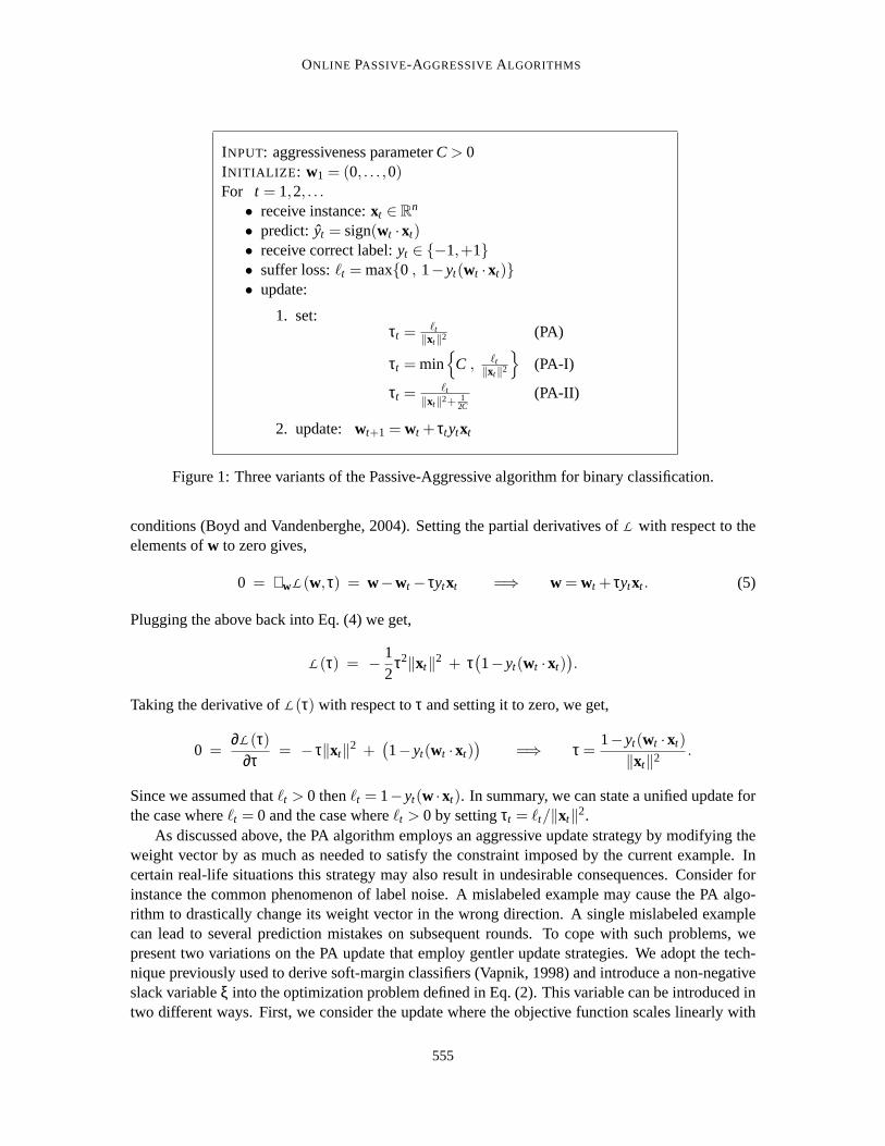
In the previous section we described a general setting for binary classification. To obtain a concretealgorithm we must determine how to initialize the weight vectorw1 and we must define the updaterule used to modify the weight vector at the end of each round. In this section we present threevariants of an online learning algorithm for binary classification. The pseudo-code for the threevariants is given in Fig. 1. The vectorw1 is initialized to(0, . . . ,0) for all three variants, howevereach variant employs a different update rule. We focus first on the simplest of the three, which onroundt sets the new weight vectorwt+1 to be the solution to the following constrained optimizationproblem,
wt+1 = argminw∈Rn
12‖w−wt‖2 s.t. ℓ(w;(xt ,yt)) = 0. (2)
Geometrically,wt+1 is set to be the projection ofwt onto the half-space of vectors which attain ahinge-loss of zero on the current example. The resulting algorithm ispassivewhenever the hinge-loss is zero, that is,wt+1 = wt wheneverℓt = 0. In contrast, on those rounds where the loss ispositive, the algorithmaggressivelyforceswt+1 to satisfy the constraintℓ(wt+1;(xt ,yt)) = 0 re-gardless of the step-size required. We therefore name the algorithmPassive-Aggressiveor PA forshort.
The motivation for this update stems from the work of Helmbold et al. (Helmbold etal., 1999)who formalized the trade-off between the amount of progress made on each round and the amountof information retained from previous rounds. On one hand, our updaterequireswt+1 to correctlyclassify the current example with a sufficiently high margin and thus progress is made. On the otherhand,wt+1 must stay as close as possible towt , thus retaining the information learned on previousrounds.
The solution to the optimization problem in Eq. (2) has a simple closed form solution,
wt+1 = wt + τtytxt where τt =ℓt
‖xt‖2 . (3)
We now show how this update is derived using standard tools from convexanalysis (see for instance(Boyd and Vandenberghe, 2004)). Ifℓt = 0 thenwt itself satisfies the constraint in Eq. (2) and isclearly the optimal solution. We therefore concentrate on the case whereℓt > 0. First, we define theLagrangian of the optimization problem in Eq. (2) to be,
L (w,τ) =12‖w−wt‖2 + τ
(
1−yt(w ·xt))
, (4)
whereτ ≥ 0 is a Lagrange multiplier. The optimization problem in Eq. (2) has a convex objectivefunction and a single feasible affine constraint. These are sufficient conditions for Slater’s conditionto hold therefore finding the problem’s optimum is equivalent to satisfying the Karush-Khun-Tucker
554
ONLINE PASSIVE-AGGRESSIVEALGORITHMS
INPUT: aggressiveness parameterC > 0INITIALIZE : w1 = (0, . . . ,0)For t = 1,2, . . .
• receive instance:xt ∈ Rn
• predict: yt = sign(wt ·xt)• receive correct label:yt ∈ {−1,+1}• suffer loss:ℓt = max{0 , 1−yt(wt ·xt)}• update:
1. set:τt = ℓt
‖xt‖2 (PA)
τt = min{
C , ℓt‖xt‖2
}
(PA-I)
τt = ℓt
‖xt‖2+ 12C
(PA-II)
2. update: wt+1 = wt + τtytxt
Figure 1: Three variants of the Passive-Aggressive algorithm for binary classification.
conditions (Boyd and Vandenberghe, 2004). Setting the partial derivatives ofL with respect to theelements ofw to zero gives,
0 = ∇wL (w,τ) = w−wt − τytxt =⇒ w = wt + τytxt . (5)
Plugging the above back into Eq. (4) we get,
L (τ) = − 12
τ2‖xt‖2 + τ(
1−yt(wt ·xt))
.
Taking the derivative ofL (τ) with respect toτ and setting it to zero, we get,
0 =∂L (τ)
∂τ= − τ‖xt‖2 +
(
1−yt(wt ·xt))
=⇒ τ =1−yt(wt ·xt)
‖xt‖2 .
Since we assumed thatℓt > 0 thenℓt = 1−yt(w ·xt). In summary, we can state a unified update forthe case whereℓt = 0 and the case whereℓt > 0 by settingτt = ℓt/‖xt‖2.
As discussed above, the PA algorithm employs an aggressive update strategy by modifying theweight vector by as much as needed to satisfy the constraint imposed by the current example. Incertain real-life situations this strategy may also result in undesirable consequences. Consider forinstance the common phenomenon of label noise. A mislabeled example may causethe PA algo-rithm to drastically change its weight vector in the wrong direction. A single mislabeled examplecan lead to several prediction mistakes on subsequent rounds. To copewith such problems, wepresent two variations on the PA update that employ gentler update strategies. We adopt the tech-nique previously used to derive soft-margin classifiers (Vapnik, 1998)and introduce a non-negativeslack variableξ into the optimization problem defined in Eq. (2). This variable can be introduced intwo different ways. First, we consider the update where the objective function scales linearly with
555
CRAMMER, DEKEL, KESHET, SHALEV-SHWARTZ AND SINGER
ξ, namely,
wt+1 = argminw∈Rn
12‖w−wt‖2 + Cξ s.t. ℓ(w;(xt ,yt)) ≤ ξ and ξ ≥ 0. (6)
HereC is a positive parameter which controls the influence of the slack term on the objective func-tion. Specifically, we will show that larger values ofC imply a more aggressive update step and wetherefore refer toC as theaggressiveness parameterof the algorithm. We term the algorithm whichresults from this updatePA-I .
Alternatively, we can have the objective function scale quadratically withξ, resulting in thefollowing constrained optimization problem,
wt+1 = argminw∈Rn
12‖w−wt‖2 + Cξ2 s.t. ℓ(w;(xt ,yt)) ≤ ξ. (7)
Note that the constraintξ ≥ 0 which appears in Eq. (6) is no longer necessary sinceξ2 is alwaysnon-negative. We term the algorithm which results from this updatePA-II . As with PA-I , C is apositive parameter which governs the degree to which the update of PA-IIis aggressive. The updatesof PA-I and PA-II also share the simple closed formwt+1 = wt + τtytxt , where
τt = min
{
C ,ℓt
‖xt‖2
}
(PA-I) or τt =ℓt
‖xt‖2 + 12C
(PA-II). (8)
A detailed derivation of the PA-I and PA-II updates is provided in Appendix A. It is worth notingthat the PA-II update is equivalent to increasing the dimension of eachxt from n to n+ T, settingxn+t =
√
1/2C, setting the remainingT − 1 new coordinates to zero, and then using the simplePA update. This technique was previously used to derive noise-tolerantonline algorithms in (Klas-ner and Simon, 1995; Freund and Schapire, 1999). We do not use this observation explicitly in thispaper, since it does not lead to a tighter analysis.
Up until now, we have restricted our discussion to linear predictors of the form sign(w ·x). Wecan easily generalize any of the algorithms presented in this section using Mercer kernels. Simplynote that for all three PA variants,
wt =t−1
∑i=1
τtytxt ,
and therefore,
wt ·xt =t−1
∑i=1
τtyt(xi ·xt).
The inner product on the right hand side of the above can be replaced with a general Mercer kernelK(xi ,xt) without otherwise changing our derivation. Additionally, the formal analysis presented inthe next section also holds for any kernel operator.
4. Analysis
In this section we proverelative loss bounds for the three variants of the PA algorithm presented inthe previous section. Specifically, most of the theorems in this section relate thecumulative squaredloss attained by our algorithms on any sequence of examples with the loss attained by an arbitrary
556
ONLINE PASSIVE-AGGRESSIVEALGORITHMS
fixed classification function of the form sign(u ·x) on the same sequence. As previously mentioned,the cumulative squared hinge loss upper bounds the number of prediction mistakes. Our boundsessentially prove that, for any sequence of examples, our algorithms cannot do much worse than thebest fixed predictor chosen in hindsight.
To simplify the presentation we use two abbreviations throughout this paper.As before wedenote byℓt the instantaneous loss suffered by our algorithm on roundt. In addition, we denoteby ℓ⋆
t the loss suffered by the arbitrary fixed predictor to which we are comparing our performance.Formally, letu be an arbitrary vector inRn, and define
ℓt = ℓ(
wt ;(xt ,yt))
and ℓ⋆t = ℓ
(
u;(xt ,yt))
. (9)
We begin with a technical lemma which facilitates the proofs in this section. With this lemmahandy, we then derive loss and mistake bounds for the variants of the PA algorithm presented in theprevious section.
Lemma 1 Let(x1,y1), . . . ,(xT ,yT) be a sequence of examples wherext ∈Rn and yt ∈ {+1,−1} for
all t. Let τt be as defined by either of the three PA variants given in Fig. 1. Then using the notationgiven in Eq. (9), the following bound holds for anyu ∈ R
n,
T
∑t=1
τt(
2ℓt − τt‖xt‖2−2ℓ⋆t
)
≤ ‖u‖2.
Proof Define∆t to be‖wt −u‖2−‖wt+1−u‖2. We prove the lemma by summing∆t over all tin 1, . . . ,T and bounding this sum from above and below. First note that∑t ∆t is a telescopic sumwhich collapses to,
T
∑t=1
∆t =T
∑t=1
(
‖wt −u‖2−‖wt+1−u‖2)
= ‖w1−u‖2−‖wT+1−u‖2.
Using the facts thatw1 is defined to be the zero vector and that‖wT+1−u‖2 is non-negative, wecan upper bound the right-hand side of the above by‖u‖2 and conclude that,
T
∑t=1
∆t ≤ ‖u‖2. (10)
We now turn to bounding∆t from below. If the minimum margin requirement is not violated onroundt, i.e. ℓt = 0, thenτt = 0 and therefore∆t = 0. We can therefore focus only on rounds forwhich ℓt > 0. Using the definitionwt+1 = wt +ytτtxt , we can write∆t as,
∆t = ‖wt −u‖2−‖wt+1−u‖2
= ‖wt −u‖2−‖wt −u+ytτtxt‖2
= ‖wt −u‖2−(
‖wt −u‖2 +2τtyt(wt −u) ·xt + τ2t ‖xt‖2)
= −2τtyt(wt −u) ·xt − τ2t ‖xt‖2. (11)
557
CRAMMER, DEKEL, KESHET, SHALEV-SHWARTZ AND SINGER
Since we assumed thatℓt > 0 thenℓt = 1−yt(wt ·xt) or alternativelyyt(wt ·xt) = 1−ℓt . In addition,the definition of the hinge loss implies thatℓ⋆
t ≥ 1−yt(u ·xt), henceyt(u ·xt) ≥ 1− ℓ⋆t . Using these
two facts back in Eq. (11) gives,
∆t ≥ 2τt ((1− ℓ⋆t )− (1− ℓt))− τ2
t ‖xt‖2
= τt(
2ℓt − τt‖xt‖2−2ℓ⋆t
)
. (12)
Summing∆t over allt and comparing the lower bound of Eq. (12) with the upper bound in Eq. (10)proves the lemma.
We first prove a loss bound for the PA algorithm in the separable case. This bound was previ-ously presented by Herbster (2001) and is analogous to the classic mistakebound for the Perceptronalgorithm due to Novikoff (1962). We assume that there exists someu ∈ R
n such thatyt(u ·xt) > 0for all t ∈ {1, . . . ,T}. Without loss of generality we can assume thatu is scaled such that thatyt(u · xt) ≥ 1 and thereforeu attains a loss of zero on allT examples in the sequence. With thevectoru at our disposal, we prove the following bound on the cumulative squared loss of PA .
Theorem 2 Let (x1,y1), . . . ,(xT ,yT) be a sequence of examples wherext ∈ Rn, yt ∈ {+1,−1} and
‖xt‖ ≤R for all t. Assume that there exists a vectoru such thatℓ⋆t = 0 for all t. Then, the cumulative
squared loss of PA on this sequence of examples is bounded by,
T
∑t=1
ℓ2t ≤ ‖u‖2R2.
Proof Sinceℓ⋆t = 0 for all t, Lemma 1 implies that,
T
∑t=1
τt(
2ℓt − τt‖xt‖2) ≤ ‖u‖2. (13)
Using the definition ofτt for the PA algorithm in the left-hand side of the above gives,
T
∑t=1
ℓ2t /‖xt‖2 ≤ ‖u‖2.
Now using the fact that‖xt‖2 ≤ R2 for all t, we get,
T
∑t=1
ℓ2t /R2 ≤ ‖u‖2.
Multiplying both sides of this inequality byR2 gives the desired bound.
The remaining bounds we prove in this section do not depend on a separability assumption.In contrast to the assumptions of Thm. 2, the vectoru which appears in the theorems below is anarbitrary vector inRn and not necessarily a perfect separator. The first of the following theoremsbounds the cumulative squared loss attained by the PA algorithm in the specialcase where all of
558

ONLINE PASSIVE-AGGRESSIVEALGORITHMS
the instances in the input sequence are normalized so that‖xt‖2 = 1. Although this assumptionis somewhat restrictive, it is often the case in many practical applications of classification that theinstances are normalized. For instance, certain kernel operators, such as the Gaussian kernel, implythat all input instances have a unit norm. See for example (Cristianini and Shawe-Taylor, 2000).
Theorem 3 Let (x1,y1), . . . ,(xT ,yT) be a sequence of examples wherext ∈ Rn, yt ∈ {+1,−1} and
‖xt‖ = 1 for all t. Then for any vectoru ∈ Rn the cumulative squared loss of PA on this sequence
of examples is bounded from above by,
T
∑t=1
ℓ2t ≤
(
‖u‖+2√
∑Tt=1(ℓ
⋆t )2
)2
.
Proof In the special case where‖xt‖2 = 1, τt andℓt are equal. Therefore, Lemma 1 gives us that,
T
∑t=1
ℓ2t ≤ ‖u‖2 +2
T
∑t=1
ℓtℓ⋆t .
Using the Cauchy-Schwartz inequality to upper bound the right-hand side of the above inequality,and denoting
LT =√
∑Tt=1ℓ2
t and UT =√
∑Tt=1(ℓ
⋆t )2, (14)
we get thatL2T ≤ ‖u‖2 +2LTUT . The largest value ofLT for which this inequality is satisfied is the
larger of the two values for which this inequality holds with equality. That is, to obtain an upperbound onLT we need to find the largest root of the second degree polynomialL2
T −2UTLT −‖u‖2,which is,
UT +√
U2T +‖u‖2.
Using the fact that√
α+β ≤√α+
√
β, we conclude that
LT ≤ ‖u‖+2UT . (15)
Taking the square of both sides of this inequality and plugging in the definitionsof LT andUT fromEq. (14) gives the desired bound.
Next we turn to the analysis of PA-I . The following theorem does not provide a loss bound butrather a mistake bound for the PA-I algorithm. That is, we prove a direct bound on the number oftimesyt 6= sign(wt ·xt) without using∑ℓ2
t as a proxy.
Theorem 4 Let (x1,y1), . . . ,(xT ,yT) be a sequence of examples wherext ∈ Rn, yt ∈ {+1,−1} and
‖xt‖ ≤ R for all t. Then, for any vectoru ∈ Rn, the number of prediction mistakes made by PA-I on
this sequence of examples is bounded from above by,
max{
R2,1/C}
(
‖u‖2 +2CT
∑t=1
ℓ⋆t
)
,
where C is the aggressiveness parameter provided to PA-I (Fig. 1) .
559
CRAMMER, DEKEL, KESHET, SHALEV-SHWARTZ AND SINGER
Proof If PA-I makes a prediction mistake on roundt then ℓt ≥ 1. Using our assumption that‖xt‖2 ≤R2 and the definitionτt = min{ℓt/‖xt‖2,C}, we conclude that if a prediction mistake occursthen it holds that,
min{1/R2,C} ≤ τtℓt .
Let M denote the number of prediction mistakes made on the entire sequence. Sinceτtℓt is alwaysnon-negative, it holds that,
min{1/R2,C} M ≤T
∑t=1
τtℓt . (16)
Again using the definition ofτt , we know thatτtℓ⋆t ≤Cℓ⋆
t and thatτt‖xt‖2 ≤ ℓt . Plugging these twoinequalities into Lemma 1 gives,
T
∑t=1
τtℓt ≤ ‖u‖2 +2CT
∑t=1
ℓ⋆t . (17)
Combining Eq. (16) with Eq. (17), we conclude that,
min{1/R2,C} M ≤ ‖u‖2 +2CT
∑t=1
ℓ⋆t .
The theorem follows from multiplying both sides of the above by max{R2,1/C}.
Finally, we turn to the analysis of PA-II . As before, the proof of the following theorem is based onLemma 1.
Theorem 5 Let (x1,y1), . . . ,(xT ,yt) be a sequence of examples wherext ∈ Rn, yt ∈ {+1,−1} and
‖xt‖2 ≤R2 for all t. Then for any vectoru∈Rn it holds that the cumulative squared loss of PA-II on
this sequence of examples is bounded by,
T
∑t=1
ℓ2t ≤
(
R2 +1
2C
)
(
‖u‖2 + 2CT
∑t=1
(ℓ⋆t )
2
)
,
where C is the aggressiveness parameter provided to PA-II (Fig. 1) .
Proof Recall that Lemma 1 states that,
‖u‖2 ≥T
∑t=1
(
2τtℓt − τ2t ‖xt‖2−2τtℓ
⋆t
)
.
Definingα = 1/√
2C, we subtract the non-negative term(ατt − ℓ⋆t /α)2 from each summand on the
right-hand side of the above inequality, to get
‖u‖2 ≥T
∑t=1
(
2τtℓt − τ2t ‖xt‖2−2τtℓ
⋆t − (ατt − ℓ⋆
t /α)2)
=T
∑t=1
(
2τtℓt − τ2t ‖xt‖2−2τtℓ
⋆t −α2τ2
t +2τtℓ⋆t − (ℓ⋆
t )2/α2)
=T
∑t=1
(
2τtℓt − τ2t (‖xt‖2 +α2)− (ℓ⋆
t )2/α2) .
560
ONLINE PASSIVE-AGGRESSIVEALGORITHMS
Plugging in the definition ofα, we obtain the following lower bound,
‖u‖2 ≥T
∑t=1
(
2τtℓt − τ2t
(
‖xt‖2 +1
2C
)
−2C(ℓ⋆t )
2)
.
Using the definitionτt = ℓt/(‖xt‖2 +1/(2C)), we can rewrite the above as,
‖u‖2 ≥T
∑t=1
(
ℓ2t
‖xt‖2 + 12C
−2C(ℓ⋆t )
2
)
.
Replacing‖xt‖2 with its upper bound ofR2 and rearranging terms gives the desired bound.
We conclude this section with a brief comparison of our bounds to previouslypublished boundsfor the Perceptron algorithm. As mentioned above, the bound in Thm. 2 is equal to the bound ofNovikoff (1962) for the Perceptron in the separable case. However,Thm. 2 bounds the cumulativesquared hinge loss of PA , whereas Novikoff’s bound is on the number of prediction mistakes.Gentile (2002) proved a mistake bound for the Perceptron in the nonseparable case which can becompared to our mistake bound for PA-I in Thm. 4. Using our notation from Thm. 4, Gentile boundsthe number of mistakes made by the Perceptron by,
R2‖u‖2
2 + ∑Tt=1ℓ⋆
t +
√
R2‖u‖2 ∑Tt=1ℓ⋆
t +(
R2‖u‖2
2
)2.
At the price of a slightly loosening this bound, we can use the inequality√
a+b≤√a+
√b to get
the simpler bound,
R2‖u‖2 + ∑Tt=1ℓ⋆
t + R‖u‖√
∑Tt=1ℓ⋆
t .
With C = 1/R2, our bound in Thm. 4 becomes,
R2‖u‖2 + 2T
∑t=1
ℓ⋆t .
Thus, our bound is inferior to Gentile’s whenR‖u‖ <√
∑Tt=1ℓ⋆
t , and even then by a factor of atmost 2.
The loss bound for PA-II in Thm. 5 can be compared with the bound of Freund and Schapire(1999) for the Perceptron algorithm. Using the notation defined in Thm. 5, Freund and Schapirebound the number of incorrect predictions made by the Perceptron by,
(
R‖u‖+√
∑Tt=1(ℓ
⋆t )2
)2
.
It can be easily verified that the bound for the PA-II algorithm given in Thm. 5 exactly equals theabove bound of Freund and Schapire whenC is set to‖u‖/(2R
√
∑t(ℓ⋆t )2). Moreover, this is the
optimal choice ofC. However, we bound the cumulative squared hinge-loss of PA-II whereas thebound of Freund and Schapire is on the number of mistakes.
561

CRAMMER, DEKEL, KESHET, SHALEV-SHWARTZ AND SINGER
5. Regression
In this section we show that the algorithms described in Sec. 3 can be modified to deal with onlineregression problems. In the regression setting, every instancext is associated with a real targetvalueyt ∈ R, which the online algorithm tries to predict. On every round, the algorithm receivesan instancext ∈ R
n and predicts a target value ˆyt ∈ R using its internal regression function. Wefocus on the class of linear regression functions, that is, ˆyt = wt · xt wherewt is the incrementallylearned vector. After making a prediction, the algorithm is given the true target valueyt and suffersan instantaneous loss. We use theε-insensitive hinge loss function:
ℓε(
w;(x,y))
=
{
0 |w ·x−y| ≤ ε|w ·x−y|− ε otherwise
, (18)
whereε is a positive parameter which controls the sensitivity to prediction mistakes. Thisloss iszero when the predicted target deviates from the true target by less thanε and otherwise growslinearly with |yt −yt |. At the end of every round, the algorithm useswt and the example(xt ,yt) togenerate a new weight vectorwt+1, which will be used to extend the prediction on the next round.
We now describe how the various PA algorithms from Sec. 3 can be adaptedto learn regressionproblems. As in the case of classification, we initializew1 to (0, . . . ,0). On each round, the PAregression algorithm sets the new weight vector to be,
wt+1 = argminw∈Rn
12‖w−wt‖2 s.t. ℓε
(
w;(xt ,yt))
= 0, (19)
In the binary classification setting, we gave the PA update the geometric interpretation of projectingwt onto the linear half-space defined by the constraintℓ
(
w;(xt ,yt))
= 0. For regression problems,the set{w ∈ R
n : ℓε(w,zt) = 0} is not a half-space but rather a hyper-slab of width 2ε. Geomet-rically, the PA algorithm for regression projectswt onto this hyper-slab at the end of every round.Using the shorthandℓt = ℓε(wt ;(xt ,yt)), the update given in Eq. (19) has a closed form solutionsimilar to that of the classification PA algorithm of the previous section, namely,
wt+1 = wt +sign(yt − yt)τtxt where τt = ℓt/‖xt‖2.
We can also obtain the PA-I and PA-II variants for online regression by introducing a slackvariable into the optimization problem in Eq. (19), as we did for classification in Eq. (6) and Eq. (7).The closed form solution for these updates also comes out to bewt+1 = wt +sign(yt − yt)τtxt whereτt is defined as in Eq. (8). The derivations of these closed-form updatesare almost identical to thatof the classification problem in Sec. 3.
We now turn to the analysis of the three PA regression algorithms described above. We wouldlike to show that the analysis given in Sec. 4 for the classification algorithms also holds for theirregression counterparts. To do so, it suffices to show that Lemma 1 still holds for regression prob-lems. After obtaining a regression version of Lemma 1, regression versions of Thm. 2 throughThm. 5 follow as immediate corollaries.
Lemma 6 Let(x1,y1), . . . ,(xT ,yT) be an arbitrary sequence of examples, wherext ∈Rn and yt ∈R
for all t. Let τt be as defined in either of the three PA variants for regression problems. Then usingthe notation given in Eq. (9), the following bound holds for anyu ∈ R
n,
T
∑t=1
τt(
2ℓt − τt‖xt‖2−2ℓ⋆t
)
≤ ‖u‖2.
562
ONLINE PASSIVE-AGGRESSIVEALGORITHMS
Proof The proof of this lemma follows that of Lemma 1 and therefore subtleties which were dis-cussed in detail in that proof are omitted here. Again, we use the definition
∆t = ‖wt −u‖2−‖wt+1−u‖2
and the same argument used in Lemma 1 implies that,
T
∑t=1
∆t ≤ ‖u‖2,
We focus our attention on bounding∆t from below on those rounds where∆t 6= 0. Using therecursive definition ofwt+1, we rewrite∆t as,
∆t = ‖wt −u‖2−‖wt −u+sign(yt − yt)τtxt‖2
= −sign(yt − yt)2τt(wt −u) ·xt − τ2t ‖xt‖2
We now add and subtract the term sign(yt − yt)2τtyt from the right-hand side above to get the bound,
∆t ≥ −sign(yt − yt)2τt(wt ·xt −yt) + sign(yt − yt)2τt(u ·xt −yt) − τ2t ‖xt‖2. (20)
Sincewt ·xt = yt , we have that−sign(yt − yt)(wt ·xt −yt) = |wt ·xt −yt |. We only need to considerthe case where∆t 6= 0, soℓt = |wt ·xt −yt |− ε and we can rewrite the bound in Eq. (20) as,
∆t ≥ 2τt(ℓt + ε) + sign(yt − yt)2τt(u ·xt −yt) − τ2t ‖xt‖2.
We also know that sign(yt − yt)(u ·xt −yt) ≥−|u ·xt −yt | and that−|u ·xt −yt | ≥ −(ℓ⋆t + ε). This
enables us to further bound,
∆t ≥ 2τt(ℓt + ε) − 2τt(ℓ⋆t + ε) − τ2
t ‖xt‖2 = τt(2ℓt − τt‖xt‖2−2ℓ⋆t ).
Summing the above over allt and comparing to the upper bound discussed in the beginning of thisproof proves the lemma.
6. Uniclass Prediction
In this section we present PA algorithms for the uniclass prediction problem. This task involvespredicting a sequence of vectorsy1,y2, · · · whereyt ∈ R
n. Uniclass prediction is fundamentally dif-ferent than classification and regression as the algorithm makes predictions without first observingany external input (such as the instancext). Specifically, the algorithm maintains in its memory avectorwt ∈ R
n and simply predicts the next element of the sequence to bewt . After extending thisprediction, the next element in the sequence is revealed and an instantaneous loss is suffered. Wemeasure loss using the followingε-insensitive loss function:
ℓε(w;y) =
{
0 ‖w−y‖ ≤ ε‖w−y‖− ε otherwise
. (21)
As in the regression setting,ε is a positive user-defined parameter. If the prediction is withinε of thetrue sequence element then no loss is suffered. Otherwise the loss is proportional to the Euclidean
563
CRAMMER, DEKEL, KESHET, SHALEV-SHWARTZ AND SINGER
distance between the prediction and the true vector. At the end of each roundwt is updated in orderto have a potentially more accurate prediction on where the next element in the sequence will fall.Equivalently, we can think of uniclass prediction as the task of finding a center-pointw such that asmany vectors in the sequence fall within a radius ofε from w. At the end of this section we discussa generalization of this problem, where the radiusε is also determined by the algorithm.
As before, we initializew1 = (0, . . . ,0). Beginning with the PA algorithm, we define the updatefor the uniclass prediction algorithm to be,
wt+1 = argminw∈Rn
12‖w−wt‖2 s.t. ℓε(w;yt) = 0, (22)
Geometrically,wt+1 is set to be the projection ofwt onto a ball of radiusε aboutyt . We now showthat the closed form solution of this optimization problem turns out to be,
wt+1 =
(
1− ℓt
‖wt −yt‖
)
wt +
(
ℓt
‖wt −yt‖
)
yt . (23)
First, we rewrite the above equation and expresswt+1 by,
wt+1 = wt + τtyt −wt
‖yt −wt‖, (24)
whereτt = ℓt . In the Uniclass problem the KKT conditions are both sufficient and necessary foroptimality. Therefore, we prove that Eq. (24) is the minimizer of Eq. (22) by verifying that the KKTconditions indeed hold. The Lagrangian of Eq. (22) is,
L (w,τ) =12‖w−wt‖2 + τ(‖w−yt‖− ε) , (25)
whereτ ≥ 0 is a Lagrange multiplier. Differentiating with respect to the elements ofw and settingthese partial derivatives to zero, we get the first KKT condition, stating that at the optimum(w,τ)must satisfy the equality,
0 = ∇wL (w,τ) = w−wt + τw−yt
‖w−yt‖. (26)
In addition, an optimal solution must satisfy the conditionsτ ≥ 0 and,
τ(‖w−yt‖− ε) = 0. (27)
Clearly, τt ≥ 0. Therefore, to show thatwt+1 is the optimum of Eq. (22) it suffices to prove that(wt+1,τt) satisfies Eq. (26) and Eq. (27). These equalities trivially hold ifℓt = 0 and therefore fromnow on we assume thatℓt > 0. Plugging the valuesw = wt+1 andτ = τt in the right-hand side ofEq. (26) gives,
wt+1−wt + τtwt+1−yt
‖wt+1−yt‖= τt
(
yt −wt
‖yt −wt‖+
wt+1−yt
‖wt+1−yt‖
)
. (28)
Note that,
wt+1−yt = wt + τtyt −wt
‖yt −wt‖−yt = (wt −yt)
(
1− τt1
‖yt −wt‖
)
=wt −yt
‖wt −yt‖(‖wt −yt‖− τt) =
ε‖wt −yt‖
(wt −yt). (29)
564
ONLINE PASSIVE-AGGRESSIVEALGORITHMS
Combining Eq. (29) with Eq. (28) we get that,
wt+1−wt + τtwt+1−yt
‖wt+1−yt‖= 0,
and thus Eq. (26) holds for(wt+1,τt). Similarly,
‖wt+1−yt‖− ε = ε− ε = 0,
and thus Eq. (27) also holds. In summary, we have shown that the KKT optimality conditions holdfor (wt+1,τt) and therefore Eq. (24) gives the desired closed-form update.
To obtain uniclass versions of PA-I and PA-II , we add a slack variable tothe optimizationproblem in Eq. (22) in the same way as we did in Eq. (6) and Eq. (7) for the classification algorithms.Namely, the update for PA-I is defined by,
wt+1 = argminw∈Rn
12‖w−wt‖2 +Cξ s.t. ‖w−yt‖ ≤ ε+ξ, ξ ≥ 0, (30)
and the update for PA-II is,
wt+1 = argminw∈Rn
12‖w−wt‖2 +Cξ2 s.t. ‖w−yt‖ ≤ ε+ξ.
The closed form for these updates can be derived using the same technique as we used forderiving the PA update. The final outcome is that both PA-I and PA-II share the form of updategiven in Eq. (24), withτt set to be,
τt = min{ C , ℓt } (PA-I) or τt =ℓt
1+ 12C
(PA-II).
We can extend the analysis of the three PA variants from Sec. 4 to the case of uniclass prediction.We do so by proving a uniclass version of Lemma 1. After proving this lemma, wediscuss anadditional technical difficulty which needs to be addressed so that Thm. 2 through Thm. 5 carryover smoothly to the uniclass case.
Lemma 7 Let y1, . . . ,yT be an arbitrary sequence of vectors, whereyt ∈ Rn for all t. Let τt be as
defined in either of the three PA variants for uniclass prediction. Then usingthe notation given inEq. (9), the following bound holds for anyu ∈ R
n,
T
∑t=1
τt (2ℓt − τt −2ℓ⋆t ) ≤ ‖u‖2.
Proof We prove this lemma in much the same way as we did Lemma 1. We again use the definition,∆t = ‖wt −u‖2−‖wt+1−u‖2, along with the fact stated in Eq. (10) that
T
∑t=1
∆t ≤ ‖u‖2.
565
CRAMMER, DEKEL, KESHET, SHALEV-SHWARTZ AND SINGER
We now focus our attention on bounding∆t from below on those rounds where∆t 6= 0. Using therecursive definition ofwt+1, we rewrite∆t as,
∆t = ‖wt −u‖2−∥
∥
∥
∥
(
1− τt
‖wt −yt‖
)
wt +
(
τt
‖wt −yt‖
)
yt −u
∥
∥
∥
∥
2
= ‖wt −u‖2−∥
∥
∥
∥
(wt −u)+
(
τt
‖wt −yt‖
)
(yt −wt)
∥
∥
∥
∥
2
= −2
(
τt
‖wt −yt‖
)
(wt −u) · (yt −wt) − τ2t .
We now add and subtractyt from the term(wt −u) above to get,
∆t = −2
(
τt
‖wt −yt‖
)
(wt −yt +yt −u) · (yt −wt) − τ2t
= 2τt‖wt −yt‖ − 2
(
τt
‖wt −yt‖
)
(yt −u) · (yt −wt) − τ2t .
Now, using the Cauchy-Schwartz inequality on the term(yt −u) · (yt −wt), we can bound,
∆t ≥ 2τt‖wt −yt‖ − 2τt‖yt −u‖ − τ2t .
We now add and subtract 2τtε from the right-hand side of the above, to get,
∆t ≥ 2τt (‖wt −yt‖− ε) − 2τt (‖yt −u‖− ε) − τ2t .
Since we are dealing with the case whereℓt > 0, it holds thatℓt = ‖wt − yt‖− ε. By definition,ℓ⋆t ≥ ‖u−yt‖− ε. Using these two facts, we get,
∆t ≥ 2τtℓt −2τtℓ⋆t − τ2
t .
Summing the above inequality over allt and comparing the result to the upper bound in Eq. (10)gives the bound stated in the lemma.
As mentioned above, there remains one more technical obstacle which standsin the way ofapplying Thm. 2 through Thm. 5 to the uniclass case. This difficulty stems from the factxt is notdefined in the uniclass whereas the term‖x‖2 appears in the theorems. This issue is easily resolvedby settingxt in the uniclass case to be an arbitrary vector of a unit length, namely‖xt‖2 = 1. Thistechnical modification enables us to writeτt as ℓt/‖xt‖2 in the uniclass PA algorithm, as in theclassification case. Similarly,τt can be defined as in the classification case for PA-I and PA-II .Now Thm. 2 through Thm. 5 can be applied verbatim to the uniclass PA algorithms.
Learning the Radius of the Uniclass Predictor In the derivation above we made the simplifyingassumption thatε, the radius of our uniclass predictor, is fixed beforehand and that the online algo-rithm can only move its center,w. We now show that learningε andw in parallel is no harder thanlearningw alone. We do so by using a simple reduction argument. For technical reasons, we stillrequire an upper bound onε, which we denote byB. AlthoughB is specified ahead of time, it can
566
ONLINE PASSIVE-AGGRESSIVEALGORITHMS
be arbitrarily large and does not appear in our analysis. Typically, we willthink of B as being fargreater than any conceivable value ofε. Our goal is now to incrementally findwt andεt such that,
‖wt −yt‖ ≤ εt , (31)
as often as possible. Additionally, we would likeεt to stay relatively small, since an extremelylarge value ofεt would solve the problem in a trivial way. We do so by reducing this problem toadifferent uniclass problem where the radius is fixed and whereyt is in R
n+1. That is, by adding anadditional dimension to the problem, we can learnε using the same machinery developed for fixed-radius uniclass problems. The reduction stems from the observation that Eq. (31) can be writtenequivalently as,
‖wt −yt‖2 +(B2− ε2t ) ≤ B2. (32)
If we were to concatenate a 0 to the end of everyyt (thus increasing its dimension ton+ 1) andif we considered then+ 1’th coordinate ofwt to be equivalent to
√
B2− ε2t , then Eq. (32) simply
becomes‖wt −yt‖2 ≤ B2. Our problem has reduced to a fixed-radius uniclass problem where theradius is set toB. w1,n+1 should be initialized toB, which is equivalent to initializingε1 = 0. Oneach round,εt can be extracted fromwt by,
εt =√
B2−w2t,n+1.
Sincewt+1,n+1 is defined to be a convex combination ofwt,n+1 andyt,n+1 (where the latter equalszero), thenwt,n+1 is bounded in(0,B] for all t and can only decrease from round to round. Thismeans that the radiusεt is always well defined and can only increase witht. Since the radius isinitialized to zero and is now one of the learned parameters, the algorithm has anatural tendencyto favor small radii. Letu denote the center of a fixed uniclass predictor and letε denote its radius.Then the reduction described above enables us to prove loss bounds similar to those presented inSec. 4, with‖u‖2 replaced by‖u‖2 + ε2.
7. Multiclass Problems
We now address more complex decision problems. We first adapt the binaryclassification algo-rithms described in Sec. 3 to the task ofmulticlass multilabelclassification. In this setting, everyinstance is associated with a set of labelsYt . For concreteness we assume that there arek differentpossible labels and denote the set of all possible labels byY = {1, . . . ,k}. For every instancext , theset of relevant labelsYt is therefore a subset ofY . We say that labely is relevantto the instancext ify∈Yt . This setting is often discussed in text categorization applications (see for instance (Schapireand Singer, 2000)) wherext represents a document andYt is the set of topics which are relevant tothe document and is chosen from a predefined collection of topics. The special case where thereis only asingle relevant topic for each instance is typically referred to asmulticlass single-labelclassification or multiclass categorization for short. As discussed below, our adaptation of the PAvariants to multiclass multilabel settings encompasses the single-label setting as a special case.
As in the previous sections, the algorithm receives instancesx1,x2, . . . in a sequential mannerwhere eachxt belongs to an instance spaceX . Upon receiving an instance, the algorithm outputsa score for each of thek labels inY . That is, the algorithm’s prediction is a vector inR
k whereeach element in the vector corresponds to the score assigned to the respective label. This formof prediction is often referred to as label ranking. Predicting a label ranking is more general and
567
CRAMMER, DEKEL, KESHET, SHALEV-SHWARTZ AND SINGER
flexible than predicting the set of relevant labelsYt . Special purpose learning algorithms such asAdaBoost.MR (Schapire and Singer, 1998) and adaptations of supportvector machines (Crammerand Singer, 2003a) have been devised for the task of label ranking. Here we describe a reductionfrom online label ranking to online binary classification that deems label ranking as simple as binaryprediction. We note that in the case of multiclass single-label classification, theprediction of thealgorithm is simply set to be the label with the highest score.
For a pair of labelsr,s∈ Y , if the score assigned by the algorithm to labelr is greater than thescore assigned to labels, we say that labelr is rankedhigher than labels. The goal of the algorithmis to rank every relevant label above every irrelevant label. Assume that we are provided with a setof d featuresφ1, . . . ,φd where each featureφ j is a mapping fromX × Y to the reals. We denoteby Φ(x,y) = (φ1(x,y), . . . ,φd(x,y)) the vector formed by concatenating the outputs of the features,when each feature is applied to the pair(x,y). The label ranking function discussed in this sectionis parameterized by a weight vector,w ∈ R
d. On roundt, the prediction of the algorithm is thek-dimensional vector,
(
(wt ·Φ(xt ,1)) , . . . , (wt ·Φ(xt ,k)))
.
We motivate our construction with an example from the domain of text categorization. We describea variant of theTerm Frequency - Inverse Document Frequency(TF-IDF) representation of docu-ments (Rocchio, 1971; Salton and Buckley, 1988). Each featureφ j corresponds to a different word,denotedµj . Given a corpus of documentsS, for everyx ∈ S and for every potential topicy, thefeatureφ j(x,y) is defined to be,
φ j(x,y) = TF(µj ,x) · log
( |S|DF(µj ,y)
)
,
where TF(µj ,x) is the number of timesµj appears inx and DF(µj ,y) is the number of timesµj
appears in all of the documents inSwhich arenot labeled byy. The valueφ j grows in proportion tothe frequency ofµj in the documentx but is dampened ifµj is a frequent word for topics other thany. In the context of this paper, the important point is that each feature is label-dependent.
After making its prediction (a ranking of the labels), the algorithm receives the correct set ofrelevant labelsYt . We define themarginattained by the algorithm on roundt for the example(xt ,Yt)as,
γ(
wt ;(xt ,Yt))
= minr∈Yt
wt ·Φ(xt , r) − maxs6∈Yt
wt ·Φ(xt ,s).
This definition generalizes the definition of margin for binary classification and was employed byboth single-label and multilabel learning algorithms for support vector machines (Vapnik, 1998;Weston and Watkins, 1999; Elisseeff and Weston, 2001; Crammer and Singer, 2003a). In words,the margin is the difference between the score of the lowest ranked relevant label and the scoreof the highest ranked irrelevant label. The margin is positive only if all of the relevant labels areranked higher than all of the irrelevant labels. However, in the spirit of binary classification, we arenot satisfied by a mere positive margin as we require the margin of every prediction to be at least 1.After receivingYt , we suffer an instantaneous loss defined by the following hinge-loss function,
ℓMC
(
w;(x,Y))
=
{
0 γ(
w;(x,Y))
≥ 11− γ
(
w;(x,Y))
otherwise. (33)
568
ONLINE PASSIVE-AGGRESSIVEALGORITHMS
As in the previous sections, we useℓt as an abbreviation forℓMC
(
wt ;(xt ,Yt))
. If an irrelevant label isranked higher than a relevant label, thenℓ2
t attains a value greater than 1. Therefore,∑Tt=1ℓ2
t upperbounds the number of multiclass prediction mistakes made on rounds 1 throughT.
One way of updating the weight vectorwt is to mimic the derivation of the PA algorithm forbinary classification defined in Sec. 3 and to set
wt+1 = argminw∈Rd
12‖w−wt‖2 s.t. ℓMC(w;(xt ,Yt)) = 0. (34)
Satisfying the single constraint in the optimization problem above is equivalentto satisfying thefollowing set of linear constraints,
∀r ∈Yt ∀s 6∈Yt w ·Φ(xt , r)−w ·Φ(xt ,s) ≥ 1. (35)
However, instead of attempting to satisfy all of the|Y t |× (k−|Y t |) constraints above we focus onlyon the single constraint which is violated the most bywt . We show in the sequel that we can stillprove a cumulative loss bound for this simplified version of the update. We note that satisfying allof these constraints simultaneously leads to the online algorithm presented in (Crammer and Singer,2003a). Their online update is more involved and computationally expensive, and moreover, theiranalysis only covers the realizable case.
Formally, let rt denote the lowest ranked relevant label and letst denote the highest rankedirrelevant label on roundt. That is,
rt = argminr∈Yt
wt ·Φ(xt , r) and st = argmaxs6∈Yt
wt ·Φ(xt ,s). (36)
The single constraint that we choose to satisfy isw ·Φ(xt , rt)−w ·Φ(xt ,st) ≥ 1 and thuswt+1 is setto be the solution of the following simplified constrained optimization problem,
wt+1 = argminw
12‖w−wt‖2 s.t. w · (Φ(xt , rt)−Φ(xt ,st)) ≥ 1. (37)
The apparent benefit of this simplification lies in the fact that Eq. (37) has aclosed form solution.To draw the connection between the multilabel setting and binary classification,we can think of thevectorΦ(xt , rt)−Φ(xt ,st) as a virtual instance of a binary classification problem with a label of+1. With this reduction in mind, Eq. (37) becomes equivalent to Eq. (2). Therefore, the closed formsolution of Eq. (37) is
wt+1 = wt + τt(Φ(xt , rt)−Φ(xt ,st)). (38)
with,
τt =ℓt
‖Φ(xt , rt)−Φ(xt ,st)‖2 .
Although we are essentially neglecting all but two labels on each step of the multiclass update, wecan still obtain multiclass cumulative loss bounds. The key observation in our analysis it that,
ℓMC
(
wt ;(xt ,Yt))
= ℓ(
wt ;(Φ(xt , rt)−Φ(xt ,st),+1))
.
To remind the reader,ℓ on the right-hand side of the above equation is the binary classification lossdefined in Eq. (1). Using this equivalence of definitions, we can convert Thm. 2 into a bound for
569
CRAMMER, DEKEL, KESHET, SHALEV-SHWARTZ AND SINGER
the multiclass PA algorithm. To do so we need to cast the assumption that for allt it holds that‖Φ(xt , rt)−Φ(xt ,st)‖ ≤ R. This bound can immediately be converted into a bound on the normof the feature set since‖Φ(xt , rt)−Φ(xt ,st)‖ ≤ ‖Φ(xt , rt)‖+‖Φ(xt ,st)‖. Thus, if the norm of themappingΦ(xt , r) is bounded for allt and r then so is‖Φ(xt , rt)−Φ(xt ,st)‖. In particular, if weassume that‖Φ(xt , r)‖ ≤ R/2 for all t andr we obtain the following corollary.
Corollary 8 Let (x1,Y1), . . . ,(xT ,YT) be a sequence of examples withxt ∈ Rn and YT ⊆ {1, . . . ,k}.
Let Φ be a mappingΦ : X ×Y → Rd such that‖Φ(xt , r)‖ ≤ R/2 for all t and r. Assume that there
exists a vectoru such thatℓ(u;(xt ,Yt)) = 0 for all t. Then, the cumulative squared loss attained bythe multiclass multilabel PA algorithm is bounded from above by,
T
∑t=1
ℓ2t ≤ R2‖u‖2.
Similarly, we can obtain multiclass versions of PA-I and PA-II by using the update rule in Eq. (38)but settingτt to be either,
τt = min
{
C ,ℓt
‖Φ(xt , rt)−Φ(xt ,st)‖2
}
or τt =ℓt
‖Φ(xt , rt)−Φ(xt ,st)‖2 + 12C
,
respectively. The analysis of PA-I and PA-II in Thms. 4-5 also carriesover from the binary case tothe multilabel case in the same way.
Multi-prototype Classification In the above discussion we assumed that the feature vectorΦ(x,y)is label-dependent and used a single weight vectorw to form the ranking function. However, inmany applications of multiclass classification this setup is somewhat unnatural. Many times, thereis a single natural representation for every instance rather than multiple feature representations foreach individual class. For example, in optical character recognition problems (OCR) an instancecan be a gray-scale image of the character and the goal is to output the content of this image. In thisexample, it is difficult to find a good set of label-dependent features.
The common construction in such settings is to assume that each instance is a vector in Rn and to
associate a different weight vector (often referred to as prototype) with each of thek labels (Vapnik,1998; Weston and Watkins, 1999; Crammer and Singer, 2001). That is, the multiclass predictor isnow parameterized byw1
t , . . . ,wkt , wherewr
t ∈ Rn. The output of the predictor is defined to be,
(
(w1t ·xt), . . . ,(wk
t ·xt))
.
To distinguish this setting from the previous one we refer to this setting as the multi-prototype mul-ticlass setting and to the previous one as the single-prototype multiclass setting. We now describea reduction from the multi-prototype setting to the single-prototype one which enables us to use allof the multiclass algorithms discussed above in the multi-prototype setting as well. Toobtain thedesired reduction, we must define the feature vector representationΦ(x,y) induced by the instancelabel pair(x,y). We defineΦ(x,y) to be ak·n dimensional vector which is composed ofk blocks ofsizen. All blocks but they’th block of Φ(x,y) are set to be the zero vector while they’th block is setto bex. Applying a single prototype multiclass algorithm to this problem produces a weight vectorwt ∈R
kn on every online round. Analogous to the construction ofΦ(x,y), the vectorwt is composed
570
ONLINE PASSIVE-AGGRESSIVEALGORITHMS
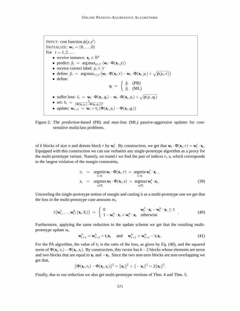
INPUT: cost functionρ(y,y′)INITIALIZE : w1 = (0, . . . ,0)For t = 1,2, . . .
• receive instance:xt ∈ Rn
• predict: yt = argmaxy∈Y (wt ·Φ(xt ,y))• receive correct label:yt ∈ Y• define:yt = argmaxr∈Y
(
wt ·Φ(xt , r)−wt ·Φ(xt ,yt)+√
ρ(yt , r))
• define:
qt =
{
yt (PB)yt (ML)
• suffer loss:ℓt = wt ·Φ(xt ,qt)−wt ·Φ(xt ,yt)+√
ρ(yt ,qt)• set:τt = ℓt
‖Φ(xt ,yt)−Φ(xt ,qt)‖2
• update:wt+1 = wt + τt (Φ(xt ,yt)−Φ(xt ,qt))
Figure 2: Theprediction-based(PB) and max-loss(ML) passive-aggressive updates for cost-sensitive multiclass problems.
of k blocks of sizen and denote blockr by wrt . By construction, we get thatwt ·Φ(xt , r) = wr
t ·xt .Equipped with this construction we can use verbatim any single-prototype algorithm as a proxy forthe multi-prototype variant. Namely, on roundt we find the pair of indicesrt ,st which correspondsto the largest violation of the margin constraints,
rt = argminr∈Yt
wt ·Φ(xt , r) = argminr∈Yt
wrt ·xt ,
st = argmaxs6∈Yt
wt ·Φ(xt ,s) = argmaxs6∈Yt
wst ·xt . (39)
Unraveling the single-prototype notion of margin and casting it as a multi-prototype one we get thatthe loss in the multi-prototype case amounts to,
ℓ(
w1t , . . . ,w
kt ;(xt ,Yt)
)
=
{
0 wrtt ·xt −wst
t ·xt ≥ 11−wrt
t ·xt +wstt ·xt otherwise
. (40)
Furthermore, applying the same reduction to the update scheme we get that theresulting multi-prototype update is,
wrtt+1 = wrt
t+1 + τtxt and wstt+1 = wst
t+1− τtxt . (41)
For the PA algorithm, the value ofτt is the ratio of the loss, as given by Eq. (40), and the squarednorm ofΦ(xt , rt)−Φ(xt ,st). By construction, this vector hask−2 blocks whose elements are zerosand two blocks that are equal toxt and−xt . Since the two non-zero blocks are non-overlapping weget that,
‖Φ(xt , rt)−Φ(xt ,st)‖2 = ‖xt‖2 + ‖−xt‖2 = 2‖xt‖2.
Finally, due to our reduction we also get multi-prototype versions of Thm. 4 and Thm. 5.
571
CRAMMER, DEKEL, KESHET, SHALEV-SHWARTZ AND SINGER
8. Cost-Sensitive Multiclass Classification
Cost-sensitive multiclass classification is a variant of the multiclass single-labelclassification settingdiscussed in the previous section. Namely, each instancext is associated with a single correct labelyt ∈ Y and the prediction extended by the online algorithm is simply,
yt = argmaxy∈Y
(wt ·Φ(xt ,y)) . (42)
A prediction mistake occurs ifyt 6= yt , however in the cost-sensitive setting different mistakes incurdifferent levels of cost. Specifically, for every pair of labels(y,y′) there is a costρ(y,y′) associatedwith predictingy′ when the correct label isy. The cost functionρ is defined by the user and takesnon-negative values. We assume thatρ(y,y) = 0 for all y∈ Y and thatρ(y,y′) ≥ 0 whenevery 6= y′.The goal of the algorithm is to minimize thecumulative costsuffered on a sequence of examples,namely to minimize∑ρ(yt , yt).
The multiclass PA algorithms discussed above can be adapted to this task by incorporating thecost function into the online update. Recall that we began the derivation ofthe multiclass PA updateby defining a set of margin constraints in Eq. (35), and on every round we focused our attentionon satisfying only one of these constraints. We repeat this idea here while incorporating the costfunction into the margin constraints. Specifically, on every online round we would like for thefollowing constraints to hold,
∀r ∈ {Y \yt} wt ·Φ(xt ,yt)−wt ·Φ(xt , r) ≥√
ρ(yt , r). (43)
The reason for using the square root function in the equation above will be justified shortly. Asmentioned above, the online update focuses on a single constraint out of the |Y |−1 constraints inEq. (43). We will describe and analyze two different ways to choose thissingle constraint, whichlead to two different online updates for cost-sensitive classification. Thetwo update techniques arecalled theprediction-basedupdate and themax-lossupdate. Pseudo-code for these two updates ispresented in Fig. 2. They share an almost identical analysis and may seem very similar at first,however each update possesses unique qualities. We discuss the significance of each update at theend of this section.
The prediction-based update focuses on the single constraint in Eq. (43) which corresponds tothe predicted label ˆyt . Concretely, this update setswt+1 to be the solution to the following optimiza-tion problem,
wt+1 = argminw∈Rn
12‖w−wt‖2 s.t. wt ·Φ(xt ,yt)−wt ·Φ(xt , yt) ≥
√
ρ(yt , yt), (44)
where yt is defined in Eq. (42). This update closely resembles the multiclass update given inEq. (37). Define the cost sensitive loss for the prediction-based update to be,
ℓPB
(
w;(x,y))
= w ·Φ(x, y)−w ·Φ(x,y)+√
ρ(y, y). (45)
Note that this loss equals zero if and only if a correct prediction was made, namely if yt = yt . Onthe other hand, if a prediction mistake occurred it means thatwt ranked ˆyt higher thanyt , thus,
√
ρ(yt , yt) ≤ wt ·Φ(xt , yt)−wt ·Φ(xt ,yt)+√
ρ(yt , yt) = ℓPB(wt ;(xt ,yt)). (46)
572
ONLINE PASSIVE-AGGRESSIVEALGORITHMS
As in previous sections, we will prove an upper bound on the cumulative squared loss attained byour algorithm,∑t ℓPB(wt ;(xt ,yt))
2. The cumulative squared loss in turn bounds∑t ρ(yt , yt) which isthe quantity we are trying to minimize. This explains the rationale behind our choiceof the marginconstraints in Eq. (43). The update in Eq. (44) has the closed form solution,
wt+1 = wt + τt (Φ(xt ,yt)−Φ(xt , yt)) , (47)
where,
τt =ℓPB(wt ;(xt ,yt))
‖Φ(xt ,yt)−Φ(xt , yt)‖2 . (48)
As before, we obtain cost sensitive versions of PA-I and PA-II by setting,
τt = min
{
C ,ℓPB(wt ;(xt ,yt))
‖Φ(xt ,yt)−Φ(xt , yt)‖2
}
(PA-I)
τt =ℓPB(wt ;(xt ,yt))
‖Φ(xt ,yt)−Φ(xt , yt)‖2 + 12C
(PA-II), (49)
where in both casesC > 0 is a user-defined parameter.The second cost sensitive update, the max-loss update, also focuses on satisfying a single con-
straint from Eq. (43). Let ˜yt be the label inY defined by,
yt = argmaxr∈Y
(
wt ·Φ(xt , r)−wt ·Φ(xt ,yt)+√
ρ(yt , r))
. (50)
yt is the loss-maximizing label. That is, we would suffer the greatest loss on round t if we were topredictyt . The max-loss update focuses on the single constraint in Eq. (43) which corresponds to ˜yt .Note that the online algorithm continues to predict the label ˆyt as before and that ˜yt only influencesthe online update. Concretely, the max-loss update setswt+1 to be the solution to the followingoptimization problem,
wt+1 = argminw∈Rn
12‖w−wt‖2 s.t. wt ·Φ(xt ,yt)−wt ·Φ(xt , yt) ≥
√
ρ(yt , yt), (51)
The update in Eq. (51) has the same closed form solution given in Eq. (47)and Eq. (48) with ˆyt
replaced by ˜yt . Define the loss for the max-loss update to be,
ℓML
(
w;(x,y))
= w ·Φ(x, y)−w ·Φ(x,y)+√
ρ(y, y), (52)
wherey is defined in Eq. (50). Note that since ˜y attains the maximal loss of all other labels, it followsthat,
ℓPB(wt ;(xt ,yt)) ≤ ℓML(wt ;(xt ,yt)).
From the above inequality and Eq. (46) we conclude thatℓML is also an upper bound on√
ρ(yt , yt).A note-worthy difference betweenℓPB andℓML is thatℓML(wt ;(xt ,yt)) = 0 if and only if Eq. (43)holds for allr ∈ {Y \yt}, whereas this is not the case forℓPB.
The prediction-based and max-loss updates were previously discussedin Dekel et al. (2004a), inthe context of hierarchical classification. In that paper, a predefinedhierarchy over the label set wasused to induce the cost functionρ. The basic online algorithm presented there used the prediction-based update, whereas the max-loss update was mentioned in the context ofa batch learning setting.
573
CRAMMER, DEKEL, KESHET, SHALEV-SHWARTZ AND SINGER
Dekel et al. (2004a) evaluated both techniques empirically and found themto be highly effective onspeech recognition and text classification tasks.
Turning to the analysis of our cost sensitive algorithms, we follow the same strategy used in theanalysis of the regression and uniclass algorithms. Namely, we begin by proving a cost sensitiveversion of Lemma 1 for both the prediction-based and the max-loss updates.
Lemma 9 Let (x1,y1), . . . ,(xT ,yT) be an arbitrary sequence of examples, wherext ∈ R and yt ∈ Yfor all t. Let u be an arbitrary vector inRn. If τt is defined as in Eq. (48) or Eq. (49) then,
T
∑t=1
τt(
2ℓPB(wt ;(xt ,yt))− τt‖Φ(xt ,yt)−Φ(xt , yt)‖2−2ℓML(u;(xt ,yt)))
≤ ‖u‖2.
If τt is defined as in Eq. (48) or Eq. (49) withyt replaced byyt then,
T
∑t=1
τt(
2ℓML(wt ;(xt ,yt))− τt‖Φ(xt ,yt)−Φ(xt , yt)‖2−2ℓML(u;(xt ,yt)))
≤ ‖u‖2.
Proof We prove the first statement of the lemma, which involves the prediction-basedupdate rule.The proof of the second statement is identical, except that ˆyt is replaced by ˜yt andℓPB(wt ;(xt ,yt)) isreplaced byℓML(wt ;(xt ,yt)).
As in the proof of Lemma 1, we use the definition∆t = ‖wt −u‖2−‖wt+1−u‖2 and the factthat,
T
∑t=1
∆t ≤ ‖u‖2. (53)
We focus our attention on bounding∆t from below. Using the recursive definition ofwt+1, werewrite∆t as,
∆t = ‖wt −u‖2−‖wt −u+ τt(Φ(xt ,yt)−Φ(xt , yt))‖2
= −2τt(wt −u) · (Φ(xt ,yt)−Φ(xt , yt)) − τ2t ‖Φ(xt ,yt)−Φ(xt , yt)‖2. (54)
By definition,ℓML(u;(xt ,yt)) equals,
maxr∈Y
(
u · (Φ(xt , r)−Φ(xt ,yt))+√
ρ(yt , r))
.
SinceℓML(u;(xt ,yt)) is the maximum overY , it is clearly greater thanu · (Φ(xt , yt)−Φ(xt ,yt))+√
ρ(yt , yt). This can be written as,
u · (Φ(xt ,yt)−Φ(xt , yt)) ≥√
ρ(yt , yt)− ℓML(u;(xt ,yt)).
Plugging the above back into Eq. (54) we get,
∆t ≥ −2τtwt · (Φ(xt ,yt)−Φ(xt , yt)) + 2τt
(
√
ρ(yt , yt)− ℓML(u;(xt ,yt)))
− τ2t ‖Φ(xt ,yt)−Φ(xt , yt)‖2. (55)
574
ONLINE PASSIVE-AGGRESSIVEALGORITHMS
Rearranging terms in the definition ofℓPB, we get thatwt · (Φ(xt ,yt)−Φ(xt , yt)) =√
ρ(yt , yt)−ℓPB(wt ;(xt ,yt)). This enables us to rewrite Eq. (55) as,
∆t ≥ −2τt
(
√
ρ(yt , yt)− ℓPB(wt ;(xt ,yt)))
+
2τt
(
√
ρ(yt , yt)− ℓML(u;(xt ,yt)))
− τ2t ‖Φ(xt ,yt)−Φ(xt , yt)‖2
= τt(
2ℓPB(wt ;(xt ,yt))− τt‖Φ(xt ,yt)−Φ(xt , yt)‖2−2ℓML(u;(xt ,yt)))
.
Summing∆t over all t and comparing this lower bound with the upper bound provided in Eq. (53)gives the desired bound.
This lemma can now be used to obtain cost sensitive versions of Thms. 2,3 and5 for bothprediction-based and max-loss updates. The proof of these theorems remains essentially the same asbefore, however one cosmetic change is required:‖xt‖2 is replaced by either‖Φ(xt ,yt)−Φ(xt , yt)‖2
or ‖Φ(xt ,yt)−Φ(xt , yt)‖2 in each of the theorems and throughout their proofs. This provides cu-mulative cost bounds for the PA and PA-II cost-sensitive algorithms.
Analyzing the cost-sensitive version of PA-I requires a slightly more delicateadaptation ofThm. 4. For brevity, we prove the following theorem for the max-loss variant of the algorithmand note that the proof for the prediction-based variant is essentially identical.
We make two simplifying assumptions: first assume that‖φ(xt ,yt)−φ(xt , yt)‖ is upper boundedby 1. Second, assume thatC, the aggressiveness parameter given to the PA-I algorithm, is an upperbound on the square root of the cost functionρ.
Theorem 10 Let(x1,y1), . . . ,(xT ,yT) be a sequence of examples wherext ∈Rn, yt ∈ Y and‖φ(xt ,yt)−
φ(xt , yt)‖ ≤ 1 for all t. Let ρ be a cost function fromY × Y to R+ and let C, the aggressivenessparameter provided to the PA-I algorithm, be such that
√
ρ(yt , yt)≤C for all t. Then for any vectoru ∈ R
n, the cumulative cost obtained by the max-loss cost sensitive version of PA-I on the sequenceis bounded from above by,
T
∑t=1
ρ(yt , yt) ≤ ‖u‖2 +2CT
∑t=1
ℓML(u;(xt ,yt)).
Proof We abbreviateρt = ρ(yt , yt) andℓt = ℓML(wt ;(xt ,yt)) throughout this proof.ℓt ≥√ρt on
every roundt, as discussed in this section.τt is defined as,
τt = min
{
ℓt
‖φ(xt ,yt)−φ(xt , yt)‖2 , C
}
,
and due to our assumption on‖φ(xt ,yt)−φ(xt , yt)‖2 we get thatτt ≥ min{ℓt ,C}. Combining thesetwo facts gives,
min{ρt ,C√
ρt} ≤ τtℓt .
Using our assumption onC, we know thatC√ρt is at leastρt and thereforeρt ≤ τtℓt . Summing over
all t we get the bound,T
∑t=1
ρt ≤T
∑t=1
τtℓt . (56)
575
CRAMMER, DEKEL, KESHET, SHALEV-SHWARTZ AND SINGER
Again using the definition ofτt , we know thatτtℓML(u;(xt ,yt))≤CℓML(u;(xt ,yt)) and thatτt‖φ(xt ,yt)−φ(xt , yt)‖2 ≤ ℓt . Plugging these two inequalities into the second statement of Lemma 9 gives,
T
∑t=1
τtℓt ≤ ‖u‖2 +2CT
∑t=1
ℓML(u;(xt ,yt)). (57)
Combining Eq. (57) with Eq. (56) proves the theorem.
This concludes our analysis of the cost-sensitive PA algorithms. We wrap up this section with adiscussion on some significant differences between the prediction-based and the max-loss variantsof our cost-sensitive algorithms. Both variants utilize the same prediction function to output thepredicted label ˆyt however each variant follows a different update strategy and is evaluated withrespect to a different loss function. The loss function used to evaluate the prediction-based variantis a function ofyt andyt , whereas the loss function used to evaluate the max-loss update essentiallyignores ˆyt . In this respect, the prediction-based loss is more natural.
On the other hand, the analysis of the prediction-based variant lacks the aesthetics of the max-loss analysis. The analysis of the max-loss algorithm usesℓML to evaluate both the performance ofthe algorithm and the performance ofu, while the analysis of the prediction-based algorithm usesℓPB to evaluate the algorithm andℓML to evaluateu. The prediction-based relative bound is to someextent like comparing apples and oranges, since the algorithm andu are not evaluated using thesame loss function. In summary, both algorithms suffer from some theoreticaldisadvantage andneither of them is theoretically superior to the other.
Finally, we turn our attention to an important algorithmic difference between the two updatestrategies. The prediction-based update has a great advantage over the max-loss update in that thecost functionρ does not play a role in determining the single constraint which the update focuses on.In some cases, this can significantly speed-up the running time required by the online update. Forexample, in the following section we exploit this property when devising algorithms for the complexproblem of sequence prediction. When reading the following section, notethat the max-loss updatecould not have been used for sequence prediction in place of the prediction-based update. This isperhaps the most significant difference between the two cost sensitive updates.
9. Learning with Structured Output
A trendy and useful application of large margin methods is learning with structured output. Inthis setting, the set of possible labels are endowed with a predefined structure. Typically, the setof labels is very large and the structure plays a key role in constructing efficient learning and in-ference procedures. Notable examples for structured label sets are graphs (in particular trees) andsequences (Collins, 2000; Altun et al., 2003; Taskar et al., 2003; Tsochantaridis et al., 2004). Wenow overview how the cost-sensitive learning algorithms described in the previous section can beadapted to structured output settings. For concreteness, we focus on an adaptation for sequence pre-diction. Our derivation however can be easily mapped to other settings of learning with structuredoutput. In sequence prediction problems we are provided with a predefined alphabetY = {1, . . . ,k}.Each input instance is associated with a label which is a sequence overY . For simplicity we assumethat the output sequence is of a fixed lengthm. Thus, on roundt, the learning algorithm receives aninstancext and then predicts an output sequenceyt ∈ Y m. Upon predicting, the algorithm receives
576
ONLINE PASSIVE-AGGRESSIVEALGORITHMS
the correct sequenceyt that is associated withxt . As in the cost-sensitive case, the learning algo-rithm is also provided with a cost functionρ : Y m× Y m → R+. The value ofρ(y,y′) representsthe cost associated with predictingy′ instead ofy. As before we assume thatρ(y,y′) equals zero ify = y′. Apart from this requirement,ρ may be any computable function. Most sequence predictionalgorithms further assume thatρ is decomposable. Specifically, a common construction (Taskaret al., 2003; Tsochantaridis et al., 2004) is achieved by defining,ρ(y,y′) = ∑m
i=1 ρ(yi ,y′i) whereρis any non-negative (local) cost overY ×Y . In contrast, we revert to a general cost function overpairs of sequences.
As in the multiclass settings discussed above, we assume that there exists a setof featuresφ1, . . . ,φd each of which takes as its input an instancex and a sequencey and outputs a real number.We again denote byΦ(x,y) the vector of features evaluated onx andy. Equipped withΦ andρ, weare left with the task of finding,
yt = argmaxy∈Y m
(wt ·Φ(xt ,y)) , (58)
on every online round. Withyt on hand, the PA update for string prediction is identical to theprediction-based update described in the previous section. However, obtaining yt in the generalcase may require as many askm evaluations ofwt ·Φ(xt ,y). This problem becomes intractable asmbecomes large. We must therefore impose some restrictions on the feature representationΦ whichwill enable us to findyt efficiently. A possible restriction on the feature representation is to assumethat each featureφ j takes the form,
φ j(xt ,y) = ψ0j (y1,xt)+
m
∑i=2
ψ j(yi ,yi−1,xt), (59)
whereψ0j andψ j are any computable functions. This construction is analogous to imposing a first
order Markovian structure on the output sequence. This form paves the way for an efficient infer-ence, i.e. solving Eq. (58), using a dynamic programming procedure. Similaryet richer structuressuch as dynamic Bayes nets can be imposed so long as the solution to Eq. (58)can be computedefficiently. We note in passing that similar representation ofΦ using efficiently computable featuresets were proposed in (Altun et al., 2003; Taskar et al., 2003; Tsochantaridis et al., 2004).
The analysis of the cost-sensitive PA updates carries over verbatim to thesequence predictionsetting. Our algorithm for learning with structured outputs was successfullyapplied to the task ofmusic to score alignment in (Shalev-Shwartz et al., 2004a).
10. Experiments
In this section we present experimental results that demonstrate differentaspects of our PA algo-rithms and their accompanying analysis. In Sec. 10.1 we start with two experiments with syntheticdata which examine the robustness of our algorithms to noise. In Sec. 10.2 weinvestigate the effectof the aggressiveness parameterC on the performance of the PA-I and PA-II algorithms. Finally,in Sec. 10.3, we compare our multiclass versions of the PA algorithms to other online algorithmsfor multiclass problems (Crammer and Singer, 2003a) on natural data sets.
The synthetic data set used in our experiments was generated as follows. First a label was chosenuniformly at random from{−1,+1}. For positive labeled examples, instances were chosen byrandomly sampling a two-dimensional Gaussian with mean(1,1) and a diagonal covariance matrix
577
CRAMMER, DEKEL, KESHET, SHALEV-SHWARTZ AND SINGER
0 0.05 0.1 0.15 0.20
0.05
0.1
0.15
0.2
0.25
0.3
0.35
0.4
Error of optimal linear classifier
Err
or
PAPA−IPA−II
0 0.05 0.1 0.15 0.20
0.5
1
1.5
Error of optimal linear classifier
Loss
PAPA−IPA−II
0 0.05 0.1 0.15 0.20
0.05
0.1
0.15
0.2
0.25
0.3
Error of optimal linear classifier
Err
or
PAPA−IPA−II
0 0.05 0.1 0.15 0.20
0.1
0.2
0.3
0.4
0.5
0.6
0.7
0.8
0.9
Error of optimal linear classifier
Loss
PAPA−IPA−II
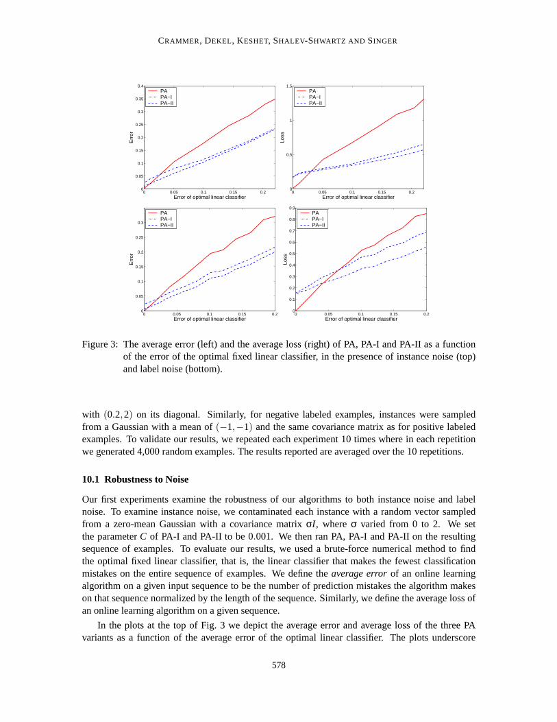
Figure 3: The average error (left) and the average loss (right) of PA,PA-I and PA-II as a functionof the error of the optimal fixed linear classifier, in the presence of instance noise (top)and label noise (bottom).
with (0.2,2) on its diagonal. Similarly, for negative labeled examples, instances were sampledfrom a Gaussian with a mean of(−1,−1) and the same covariance matrix as for positive labeledexamples. To validate our results, we repeated each experiment 10 times where in each repetitionwe generated 4,000 random examples. The results reported are averaged over the 10 repetitions.
10.1 Robustness to Noise
Our first experiments examine the robustness of our algorithms to both instance noise and labelnoise. To examine instance noise, we contaminated each instance with a random vector sampledfrom a zero-mean Gaussian with a covariance matrixσI , whereσ varied from 0 to 2. We setthe parameterC of PA-I and PA-II to be 0.001. We then ran PA, PA-I and PA-II on the resultingsequence of examples. To evaluate our results, we used a brute-forcenumerical method to findthe optimal fixed linear classifier, that is, the linear classifier that makes the fewest classificationmistakes on the entire sequence of examples. We define theaverage errorof an online learningalgorithm on a given input sequence to be the number of prediction mistakes the algorithm makeson that sequence normalized by the length of the sequence. Similarly, we define the average loss ofan online learning algorithm on a given sequence.
In the plots at the top of Fig. 3 we depict the average error and average loss of the three PAvariants as a function of the average error of the optimal linear classifier.The plots underscore
578
ONLINE PASSIVE-AGGRESSIVEALGORITHMS
−10 −8 −6 −4 −2 0 2 4 60
0.1
0.2
0.3
0.4
0.5
0.6
log(C)
Err
or
p=0.0p=0.1p=0.2
−10 −8 −6 −4 −2 0 2 4 60
0.2
0.4
0.6
0.8
1
1.2
1.4
1.6
log(C)
Loss
p=0.0p=0.1p=0.2
−10 −8 −6 −4 −2 0 2 4 60
0.1
0.2
0.3
0.4
0.5
0.6
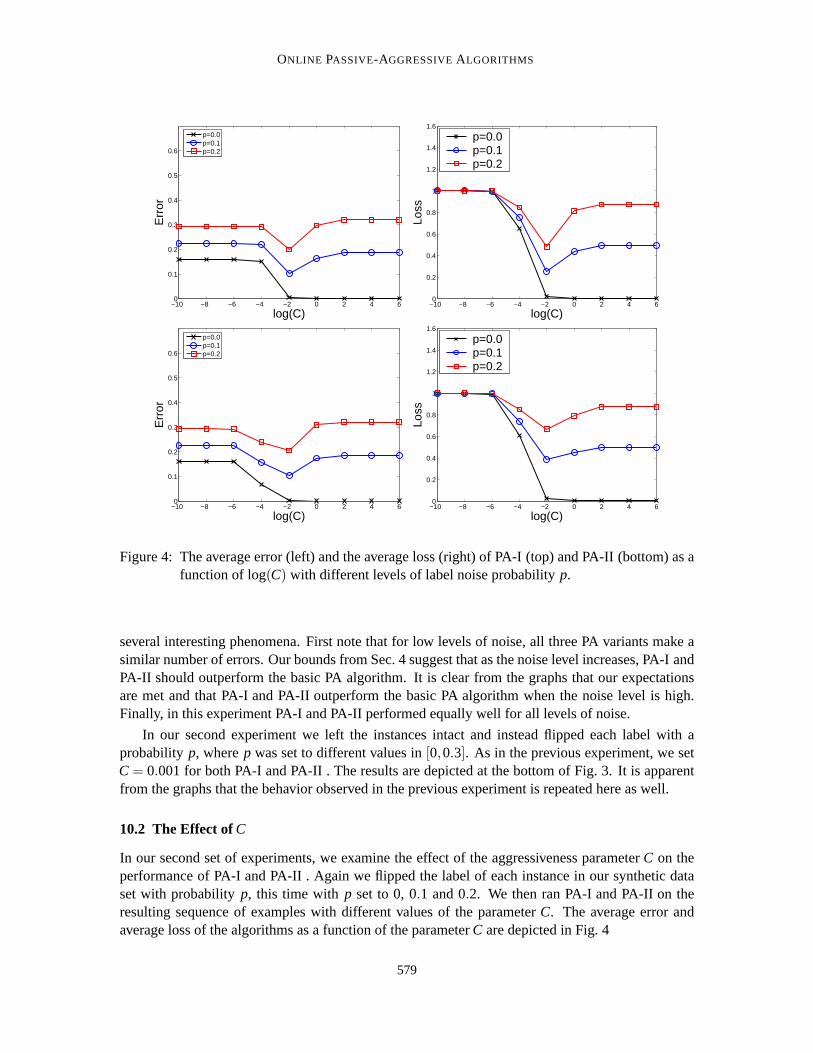
log(C)
Err
or
p=0.0p=0.1p=0.2
−10 −8 −6 −4 −2 0 2 4 60
0.2
0.4
0.6
0.8
1
1.2
1.4
1.6
log(C)
Loss
p=0.0p=0.1p=0.2
Figure 4: The average error (left) and the average loss (right) of PA-I (top) and PA-II (bottom) as afunction of log(C) with different levels of label noise probabilityp.
several interesting phenomena. First note that for low levels of noise, allthree PA variants make asimilar number of errors. Our bounds from Sec. 4 suggest that as the noise level increases, PA-I andPA-II should outperform the basic PA algorithm. It is clear from the graphs that our expectationsare met and that PA-I and PA-II outperform the basic PA algorithm when the noise level is high.Finally, in this experiment PA-I and PA-II performed equally well for all levels of noise.
In our second experiment we left the instances intact and instead flipped each label with aprobability p, wherep was set to different values in[0,0.3]. As in the previous experiment, we setC = 0.001 for both PA-I and PA-II . The results are depicted at the bottom of Fig. 3. It is apparentfrom the graphs that the behavior observed in the previous experiment isrepeated here as well.
10.2 The Effect ofC
In our second set of experiments, we examine the effect of the aggressiveness parameterC on theperformance of PA-I and PA-II . Again we flipped the label of each instance in our synthetic dataset with probabilityp, this time with p set to 0, 0.1 and 0.2. We then ran PA-I and PA-II on theresulting sequence of examples with different values of the parameterC. The average error andaverage loss of the algorithms as a function of the parameterC are depicted in Fig. 4
579
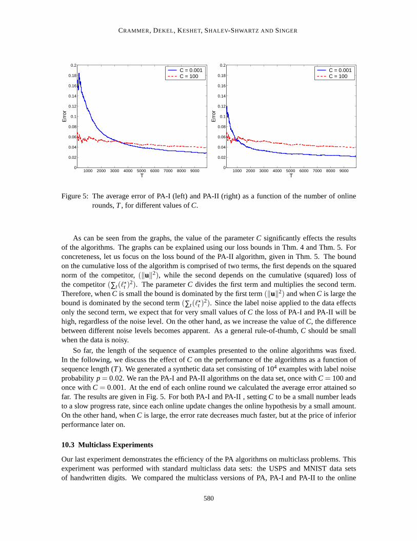
CRAMMER, DEKEL, KESHET, SHALEV-SHWARTZ AND SINGER
1000 2000 3000 4000 5000 6000 7000 8000 90000
0.02
0.04
0.06
0.08
0.1
0.12
0.14
0.16
0.18
0.2
T
Err
orC = 0.001C = 100
1000 2000 3000 4000 5000 6000 7000 8000 90000
0.02
0.04
0.06
0.08
0.1
0.12
0.14
0.16
0.18
0.2
T
Err
or
C = 0.001C = 100
Figure 5: The average error of PA-I (left) and PA-II (right) as a function of the number of onlinerounds,T, for different values ofC.
As can be seen from the graphs, the value of the parameterC significantly effects the resultsof the algorithms. The graphs can be explained using our loss bounds in Thm. 4 and Thm. 5. Forconcreteness, let us focus on the loss bound of the PA-II algorithm, given in Thm. 5. The boundon the cumulative loss of the algorithm is comprised of two terms, the first depends on the squarednorm of the competitor,(‖u‖2), while the second depends on the cumulative (squared) loss ofthe competitor(∑t(ℓ
⋆t )
2). The parameterC divides the first term and multiplies the second term.Therefore, whenC is small the bound is dominated by the first term(‖u‖2) and whenC is large thebound is dominated by the second term(∑t(ℓ
⋆t )
2). Since the label noise applied to the data effectsonly the second term, we expect that for very small values ofC the loss of PA-I and PA-II will behigh, regardless of the noise level. On the other hand, as we increase thevalue ofC, the differencebetween different noise levels becomes apparent. As a general rule-of-thumb,C should be smallwhen the data is noisy.
So far, the length of the sequence of examples presented to the online algorithms was fixed.In the following, we discuss the effect ofC on the performance of the algorithms as a function ofsequence length (T). We generated a synthetic data set consisting of 104 examples with label noiseprobability p = 0.02. We ran the PA-I and PA-II algorithms on the data set, once withC = 100 andonce withC = 0.001. At the end of each online round we calculated the average error attained sofar. The results are given in Fig. 5. For both PA-I and PA-II , settingC to be a small number leadsto a slow progress rate, since each online update changes the online hypothesis by a small amount.On the other hand, whenC is large, the error rate decreases much faster, but at the price of inferiorperformance later on.
10.3 Multiclass Experiments
Our last experiment demonstrates the efficiency of the PA algorithms on multiclass problems. Thisexperiment was performed with standard multiclass data sets: the USPS and MNIST data setsof handwritten digits. We compared the multiclass versions of PA, PA-I and PA-II to the online
580
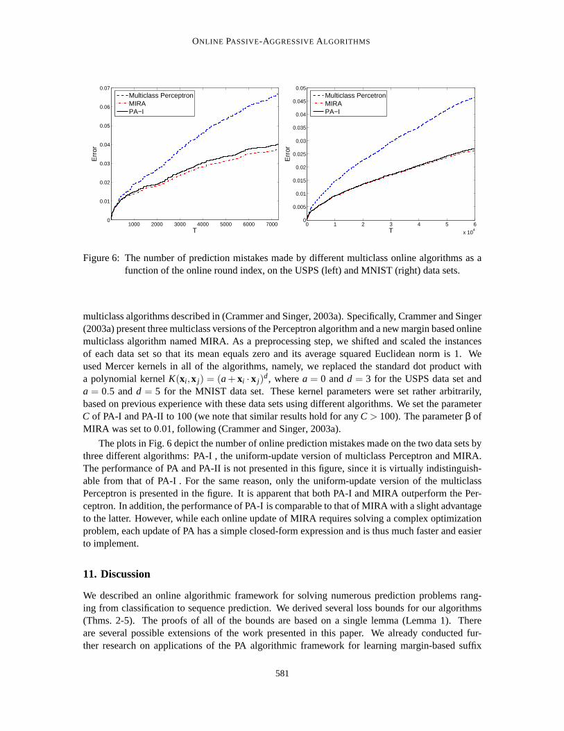
ONLINE PASSIVE-AGGRESSIVEALGORITHMS
1000 2000 3000 4000 5000 6000 70000
0.01
0.02
0.03
0.04
0.05
0.06
0.07
T
Err
orMulticlass PerceptronMIRAPA−I
0 1 2 3 4 5 6
x 104
0
0.005
0.01
0.015
0.02
0.025
0.03
0.035
0.04
0.045
0.05
T
Err
or
Multiclass PercetronMIRAPA−I
Figure 6: The number of prediction mistakes made by different multiclass onlinealgorithms as afunction of the online round index, on the USPS (left) and MNIST (right) data sets.
multiclass algorithms described in (Crammer and Singer, 2003a). Specifically,Crammer and Singer(2003a) present three multiclass versions of the Perceptron algorithm and a new margin based onlinemulticlass algorithm named MIRA. As a preprocessing step, we shifted and scaled the instancesof each data set so that its mean equals zero and its average squared Euclidean norm is 1. Weused Mercer kernels in all of the algorithms, namely, we replaced the standard dot product witha polynomial kernelK(xi ,x j) = (a+ xi · x j)
d, wherea = 0 andd = 3 for the USPS data set anda = 0.5 andd = 5 for the MNIST data set. These kernel parameters were set rather arbitrarily,based on previous experience with these data sets using different algorithms. We set the parameterC of PA-I and PA-II to 100 (we note that similar results hold for anyC > 100). The parameterβ ofMIRA was set to 0.01, following (Crammer and Singer, 2003a).
The plots in Fig. 6 depict the number of online prediction mistakes made on the two data sets bythree different algorithms: PA-I , the uniform-update version of multiclass Perceptron and MIRA.The performance of PA and PA-II is not presented in this figure, since itis virtually indistinguish-able from that of PA-I . For the same reason, only the uniform-update version of the multiclassPerceptron is presented in the figure. It is apparent that both PA-I andMIRA outperform the Per-ceptron. In addition, the performance of PA-I is comparable to that of MIRA with a slight advantageto the latter. However, while each online update of MIRA requires solving a complex optimizationproblem, each update of PA has a simple closed-form expression and is thus much faster and easierto implement.
11. Discussion
We described an online algorithmic framework for solving numerous prediction problems rang-ing from classification to sequence prediction. We derived several lossbounds for our algorithms(Thms. 2-5). The proofs of all of the bounds are based on a single lemma (Lemma 1). Thereare several possible extensions of the work presented in this paper. Wealready conducted fur-ther research on applications of the PA algorithmic framework for learning margin-based suffix
581
CRAMMER, DEKEL, KESHET, SHALEV-SHWARTZ AND SINGER
trees (Dekel et al., 2004b), pseudo-metrics (Shalev-Shwartz et al., 2004b), hierarchical classifica-tion (Dekel et al., 2004a), and segmentation of sequences (Shalev-Shwartz et al., 2004a). Whilethe focus of this paper is on online settings, online algorithms can also serve as building blocks inthe construction of well performing batch algorithms. Online to batch conversions of the proposedalgorithms are yet another important future research direction. The update taken by our algorithmsis aggressive in the sense that even a small loss forces an update of the hypothesis. When usingkernels, this property often results in the use of many examples for representing the learned predic-tor. Thus, the memory requirements imposed when using kernels can be quite demanding. We arecurrently pursuing extensions of the PA framework that operate in the realm of bounded memoryconstraints.
Acknowledgments
This research was funded by the Israeli Science Foundation under grant number 522/04. Most ofthis work was carried out at the Hebrew University of Jerusalem.
Appendix A. Derivation of the PA-I and PA-II Updates
As in Sec. 3, wheneverℓt = 0 no update occurs andτt equals zero. Ifℓt > 0 we derive theseupdates by defining the Lagrangian of the respective optimization problem and satisfying the KKTconditions. The Lagrangian of the PA-I optimization problem is,
L (w,ξ,τ,λ) =12‖w−wt‖2 + Cξ + τ(1−ξ−yt
(
w ·xt))
− λξ
=12‖w−wt‖2 + ξ(C− τ−λ) + τ(1−yt
(
w ·xt))
, (60)
whereτ ≥ 0 andλ ≥ 0 are Lagrange multipliers. We now find the minimum of the Lagrangian withrespect to the (unconstrained) primal variablesw andξ. As in the previously discussed PA update,differentiating this Lagrangian with respect to the elements ofw and setting these partial derivativesto zero gives Eq. (5) and we can writew = wt + τytxt . Next, note that the minimum of the termξ(C− τ− λ) with respect toξ is zero wheneverC− τ− λ = 0. If howeverC− τ− λ 6= 0 thenξ(C−τ−λ) can be made to approach−∞. Since we need to maximize the dual we can rule out thelatter case and pose the following constraint on the dual variables,
C− τ−λ = 0. (61)
The KKT conditions confineλ to be non-negative so we conclude thatτ ≤C. We now discuss twopossible cases: ifℓt/‖xt‖2 ≤C then we can plugging Eq. (61) back into Eq. (60) and we return tothe Lagrangian of the original PA algorithm (see Eq. (4)). From this pointand on, we can repeatthe same derivation as in the original PA update and getτt = ℓt/‖xt‖2. The other case is whenℓt/‖xt‖2 > C. This condition can be rewritten as
C‖xt‖2 < 1−yt(wt ·xt). (62)
We also know that the constraint in Eq. (6) must hold at the optimum, so 1−yt(w ·xt) ≤ ξ. Usingthe explicit form ofw given in Eq. (5), we can rewrite this constraint as 1−yt(wt ·xt)−τ‖xt‖2 ≤ ξ.
582
ONLINE PASSIVE-AGGRESSIVEALGORITHMS
Combining this inequality with the inequality in Eq. (62) gives,
C‖xt‖2− τ‖xt‖2 < ξ.
We now use our earlier conclusion thatτ ≤C to obtain 0< ξ. Turning to the KKT complementaritycondition, we know thatξλ = 0 at the optimum. Having concluded thatξ is strictly positive, we getthatλ must equal zero. Pluggingλ = 0 into Eq. (61) givesτ = C. Summing up, we used the KKTconditions to show that in the case whereℓt/‖xt‖2 > C, it is optimal to selectτ = C. Folding all ofthe possible cases into a single equation, we defineτt to be,
τt = min{
C , ℓt/‖xt‖2 } . (63)
The update of PA-I is like the update of PA clipped atC.Turning to the update of PA-II , we again recall thatℓt = 0 leads toτt = 0, and deal with those
rounds whereℓt > 0. The Lagrangian of the optimization problem in Eq. (7) equals,
L (w,ξ,τ) =12‖w−wt‖2 + Cξ2 + τ
(
1−ξ−yt(w ·xt))
, (64)
whereτ ≥ 0 is a Lagrange multiplier. Again, differentiating this Lagrangian with respectto theelements ofw and setting these partial derivatives to zero gives Eq. (5) and we can write w =wt +τytxt . Differentiating the Lagrangian with respect toξ and setting that partial derivative to zeroresults in,
0 =∂L (w,ξ,τ)
∂ξ= 2Cξ− τ =⇒ ξ =
τ2C
.
Expressingξ as above and replacingw in Eq. (60) withwt + τytxt , we rewrite the Lagrangian as,
L (τ) = − τ2
2
(
‖xt‖2 +1
2C
)
+ τ(
1−yt(wt ·xt))
.
Setting the derivative of the above to zero gives,
0 =∂L (τ)
∂τ= − τ
(
‖xt‖2 +1
2C
)
+(
1−yt(wt ·xt))
=⇒ τ =1−yt(wt ·xt)
‖xt‖2 + 12C
.
As in PA and PA-I , we can give a definition ofτt which holds in all cases,
τt =ℓt
‖x‖2 + 12C
. (65)
References
S. Agmon. The relaxation method for linear inequalities.Canadian Journal of Mathematics, 6(3):382–392, 1954.
Y. Altun, I. Tsochantaridis, and T. Hofmann. Hidden markov support vector machines. InProceed-ings of the Twentieth International Conference on Machine Learning, 2003.
S. Boyd and L. Vandenberghe.Convex Optimization. Cambridge University Press, 2004.
583
CRAMMER, DEKEL, KESHET, SHALEV-SHWARTZ AND SINGER
M. Collins. Discriminative reranking for natural language parsing. InMachine Learning: Proceed-ings of the Seventeenth International Conference, 2000.
K. Crammer and Y. Singer. On the algorithmic implementation of multiclass kernel-based vectormachines.Jornal of Machine Learning Research, 2:265–292, 2001.
K. Crammer and Y. Singer. A new family of online algorithms for category ranking. Jornal ofMachine Learning Research, 3:1025–1058, 2003a.
K. Crammer and Y. Singer. Ultraconservative online algorithms for multiclass problems.Jornal ofMachine Learning Research, 3:951–991, 2003b.
N. Cristianini and J. Shawe-Taylor.An Introduction to Support Vector Machines. Cambridge Uni-versity Press, 2000.
O. Dekel, J. Keshet, and Y. Singer. Large margin hierarchical classification. InProceedings of theTwenty-First International Conference on Machine Learning, 2004a.
O. Dekel, S. Shalev-Shwartz, and Y. Singer. The power of selective memory: Self-bounded learningof prediction suffix trees. InAdvances in Neural Information Processing Systems 17, 2004b.
A. Elisseeff and J. Weston. A kernel method for multi-labeled classification. In Advances in NeuralInformation Processing Systems 14, 2001.
Y. Freund and R. E. Schapire. Large margin classification using the perceptron algorithm.MachineLearning, 37(3):277–296, 1999.
C. Gentile. A new approximate maximal margin classification algorithm.Journal of MachineLearning Research, 2:213–242, 2001.
C. Gentile. The robustness of the p-norm algorithms.Machine Learning, 53(3), 2002.
D.P Helmbold, J. Kivinen, and M. Warmuth. Relative loss bounds for single neurons.IEEE Trans-actions on Neural Networks, 10(6):1291–1304, 1999.
M. Herbster. Learning additive models online with fast evaluating kernels.In Proceedings of theFourteenth Annual Conference on Computational Learning Theory, pages 444–460, 2001.
J. Kivinen, A. J. Smola, and R. C. Williamson. Online learning with kernels.IEEE Transactions onSignal Processing, 52(8):2165–2176, 2002.
J. Kivinen and M. Warmuth. Exponentiated gradient versus gradient descent for linear predictors.Information and Computation, 132(1):1–64, January 1997.
N. Klasner and H.U. Simon. From noise-free to noise-tolerant and from on-line to batch learning.In Proceedings of the Eighth Annual Conference on Computational Learning Theory, pages 250–264, 1995.
Y. Li and P. M. Long. The relaxed online maximum margin algorithm.Machine Learning, 46(1–3):361–387, 2002.
584
ONLINE PASSIVE-AGGRESSIVEALGORITHMS
N. Littlestone.Mistake bounds and logarithmic linear-threshold learning algorithms. PhD thesis,U. C. Santa Cruz, March 1989.
A. B. J. Novikoff. On convergence proofs on perceptrons. InProceedings of the Symposium on theMathematical Theory of Automata, volume XII, pages 615–622, 1962.
J. Rocchio. Relevance feedback information retrieval. In Gerard Salton, editor,The Smart retrievalsystem—experiments in automatic document processing, pages 313–323. Prentice-Hall, Engle-wood Cliffs, NJ, 1971.
F. Rosenblatt. The perceptron: A probabilistic model for information storage and organization inthe brain.Psychological Review, 65:386–407, 1958. (Reprinted inNeurocomputing(MIT Press,1988).).
G. Salton and C. Buckley. Term weighting approaches in automatic text retrieval. InformationProcessing and Management, 24(5), 1988.
R.E. Schapire and Y. Singer. Improved boosting algorithms using confidence-rated predictions.In Proceedings of the Eleventh Annual Conference on Computational Learning Theory, pages80–91, 1998. To appear,Machine Learning.
R.E. Schapire and Y. Singer. BoosTexter: A boosting-based system for text categorization.MachineLearning, 32(2/3), 2000.
B. Scholkopf and A. J. Smola.Learning with Kernels: Support Vector Machines, Regularization,Optimization and Beyond. MIT Press, 2002.
S. Shalev-Shwartz, J. Keshet, and Y. Singer. Learning to align polyphonic music. InProceedings of the 5th International Conference on Music Information Retrieval, 2004a.http://www.cs.huji.ac.il/∼shais/.
S. Shalev-Shwartz, Y. Singer, and A. Ng. Online and batch learning of pseudo-metrics. InProceed-ings of the Twenty-First International Conference on Machine Learning, 2004b.
B. Taskar, C. Guestrin, and D. Koller. Max-margin markov networks. InAdvances in NeuralInformation Processing Systems 17, 2003.
I. Tsochantaridis, T. Hofmann, T. Joachims, and Y. Altun. Support vector machine learning forinterdependent and structured output spaces. InProceedings of the Twenty-First InternationalConference on Machine Learning, 2004.
V. N. Vapnik. Statistical Learning Theory. Wiley, 1998.
J. Weston and C. Watkins. Support vector machines for multi-class pattern recognition. InProceed-ings of the Seventh European Symposium on Artificial Neural Networks, April 1999.
585