Online Localization of Radio-Tagged Wildlifewith an Autonomous Aerial Robot System

Oliver M. Cliff, Robert Fitch and Salah SukkariehAustralian Centre for Field Robotics

University of Sydney, Australia{o.cliff,rfitch,salah}@acfr.usyd.edu.au

Debra L. Saunders and Robert HeinsohnFenner School of Environment and Society

Australian National University, Australia{debbie.saunders,robert.heinsohn}@anu.edu.au

Abstract—The application of autonomous robots to efficientlylocate small wildlife species has the potential to provide significantecological insights not previously possible using traditional land-based survey techniques, and a basis for improved conser-vation policy and management. We present an approach forautonomously localizing radio-tagged wildlife using a small aerialrobot. We present a novel two-point phased array antennasystem that yields unambiguous bearing measurements and anassociated uncertainty measure. Our estimation and information-based planning algorithms incorporate this bearing uncertaintyto choose observation points that improve confidence in thelocation estimate. These algorithms run online in real time andwe report experimental results that show successful autonomouslocalization of stationary radio tags and live radio-tagged birds.

I. INTRODUCTION

Environmental monitoring robots can provide valuable in-formation to scientists who study natural phenomena. We areinterested in autonomous aerial robots that assist ecologists instudying animal behavior. One important application involveslocalizing animals in the wild which have been caught, in-strumented with a radio tag, and released, and periodically re-localizing the animal over weeks or months for monitoring orrecapture. Current research has made great advances in generalradio source localization, but the goal of reliably localizingwildlife autonomously and online with a flying robot remainselusive. Our aim in this paper is to take a significant steptowards this goal by demonstrating autonomous localizationof wild birds with an aerial robotic system.

Studying behavior such as the migratory patterns of variousanimal species has been of interest for over 250 years [3].Radio tag localization is used in this context instead of visualimagery due to visual occlusion by foliage. Advances insmall-scale radio frequency (RF) emitters over the past fivedecades now permits their use with small animals, such asbirds that weigh as little as 75g. However, the traditionallocalization process is largely manual and inhibits large-scaledata collection [14]. Typically a human must circle potentialtarget areas, often traveling multiple kilometers, and manuallyadjust receiver gain. The terrain may be difficult to traverseon foot. There is great opportunity for autonomous flyingsystems to improve data collection efficiency and thus help toresolve longstanding scientific questions that inform wildlifemanagement policies. It is feasible to consider the problemas one of localizing a static source because migratory animals

Fig. 1. UAV system in flight. Inset: radio-tagged Manorina Melanocephala.

often remain in an area for weeks, and often remain stationary(within a few meters) over a short time scale (minutes). Thisassumption is also made in the case of invasive fish [12].

Small aerial robots such as multirotor platforms are suitablefor this task because they are easy to deploy and can fly overterrain that is difficult to access on foot, potentially reducinglocalization time from hours in the manual case to tens ofminutes. Further, small aerial robots can operate from suffi-cient distance to not disturb wildlife. However, it is difficultto design and model a high-performance antenna system thatis light enough to be carried. Popular loop aerials [12, 28] areknown to be inefficient, especially for low frequency signals.Standard horizontally-mounted directional antennas [16, 22]are affected by unmanned aerial vehicle (UAV) rotors whichcause unpredictable irradiance.

We propose an alternative approach based on a two-pointphased array: two monopole antennas are mounted to a carrierrail, shown carried by a multirotor platform in Fig. 1. The robotperforms a full rotation to produce an unambiguous bearingmeasurement with a measure of observation uncertainty. Al-though the time duration of a single observation is roughly45s, we found that reasonable localization does not require alarge number of observations. We do not consider the detectionproblem in this work, but instead focus on localization wherea signal is present initially. Our contribution is a novel sensordesign and algorithms for autonomously locating low-power

radio tags that have been validated with live birds in the field.The target location estimate is represented by a grid-

based filter, recursively updated following each observation.The measurement bearing (and uncertainty) is obtained bydetermining the phase shift between an observed gain patternand the expected Fourier series radiation pattern model througha sliding-correlation technique. We assume that the observationbearing error is normally distributed about a bearing measure-ment, given some variable uncertainty, and consequently fusethe likelihood of each observation into the target belief. Greedyinformation-based planning is then used to plan the nextobservation point online. Estimation in the plane is sufficientin our case because the resulting estimate will generally beused to either confirm the presence of an animal in an area, orto visually locate and catch the animal for sample collection.

We present results from 22 flights and 131 observations,spanning nearly three hours of accumulated flight time. Ofthese, we performed eight manual flights for system identifi-cation and six autonomous flights localizing stationary tags inthree different areas. These results validate the performanceof the estimation process. Further, we performed three flighttrials using live birds where the robot localizes the targetwhile a human tracks its position visually. This evaluationdemonstrates the feasibility of localizing birds in the field withlow-power RF tags and a small multirotor with limited flighttime. Our results reveal the limitations of our approach at theboundary of the stationarity assumption. Finally, we discusslessons learned and extensions of our approach in practice.We expect our work to lead to further field experiments withother species and comparisons with manual methods.

II. RELATED WORK

The general problem of localizing radio-tagged wildlife hasrecently become a topic of interest in the robotics community.Significant progress has been made in solving the offlineestimation problem of localizing an RF emitter. Wagle andFrew [29] propose a Gaussian process-based method and showexperimental results from data collected by a fixed-wing UAV.Korner et al. [16] report on offline estimation experimentsusing a directional antenna and a deterministic range-bearingsensor model. Soriano et al. [26] propose a UAV system fortracking eagles that uses particle filter estimation evaluatedusing a ground-based testbed. This group has also studiedthe related problem of localizing a group of static receiversby observing a moving emitter, mounted on an autonomoushelicopter [5]. Jensen et al. [13] propose a system for trackingradio-tagged fish evaluated in simulation.

Our focus in this work is online estimation where the robotmoves autonomously and the full system is demonstratedexperimentally. The problem of designing an online estimatorfor radio localization and tracking is well studied [19, 18, 20],with emphasis on ground-based systems and an assumed sen-sor model. Extensive research in online estimation is coupledwith optimal sensor placement and planning in [7] and [10].This paper specifically addresses challenges in employing sucha system on a multirotor platform.

Fig. 2. Two-point phased array. Two monopole antennas are separated bya spacing L. This spacing causes a phase offset τ between the fore and aftantenna as a function of azimuth angle of arrival (AoA) ψ. The two signalsare summed with a combiner circuit that has an additional (constant) phaseoffset φ; this then generates a gain pattern G(ψ) ∝ 1 + cos (τ).

Pioneering achievements have been made in autonomouswildlife tracking in recent years. Hook et al. [12] analyticallysolve the problem of optimally choosing ambiguous bear-ing measurement locations for localizing a stationary target.Tokekar et al. [28] present a fully autonomous system fordetecting and localizing carp; the authors use bearing-onlymeasurements but differ significantly from our approach in im-plementation by using intersecting conical observations and apolygon belief. Moreover, the authors employ both a differentsensor model (loop antenna) and experimental platform (raft).To the best of our knowledge, ours is the first demonstrationof autonomous online localization of a live bird with a UAV.

Information-based planning has been studied for over tenyears [9]. Recent work has begun to explore sampling-basedmethods [11]. Numerous applications of information-basedplanning involve UAVs [10, 15, 21, 24, 25, 27]. In previouswork we explored multi-UAV constrained search [8] and UAVplanning using formal methods [30, 31]. Here we exploitstandard principles in greedily selecting the next observationpoint from a number of samples.

III. MULTIROTOR SENSOR MODEL

Sensor modeling is critical for successful information gath-ering; the sensor model dictates the quality of observations andtherefore directly affects the accuracy of the target estimate.An inaccurate sensor model may result in poor planningdecisions that place the robot in states where the target is lesslikely to be found or tracked. Here we present the hardwareand software components of our sensor model and discuss itsimplementation.

There are three main considerations in designing a sensormodel for a multirotor UAV: 1) multipath propagation cancause erroneous observations in cluttered environments, 2) thesensor array must balance weight and quality of readings tomaximize the number of useful observations and flight time,and 3) the rotors can cause electromagnetic interfere witha nearby antenna. We approach the first issue by remainingstationary during an observation and obtaining a bearing-only observation. The latter issues are overcome by our noveldesign of a two-point phased array system.

A. Bearing-only observation

There are two common techniques for target tracking withradio frequency (RF) beacons: range- and bearing-only obser-vations. Range-only sensor models typically are problematic incluttered environments as multipath models are undefined with

0 π/2 π 3π/2 2π0

0.5

1

ψ (rad.)

G(ψ

)

0 π/2 π 3π/2 2π0

0.5

1

ψ (rad.)

G(ψ

)

0 π/2 π 3π/2 2π−1

0

1

ψ (rad.)

ρ(G

,G)

0 π 2π0

1

0 π 2π0

1

0 π 2π0

1

Fig. 3. Illustration of the sliding-correlation waveform matching algorithm.The algorithm obtains a maximum likelihood phase offset by correlating theobserved sensor output G(ψ) against the Fourier series model G(ψ + α) :α ∈ (0, 2π]. The bottom row illustrates G shifted by α = {−π/2, π, 3π/2}.

unknown terrain, e.g., hills and valleys. Hence, we resort to abearing-only sensor model with a direction finding antenna.

Direction finding antennas are used to passively determinethe angle of arrival (AoA) of an emitting source [6]. Most tech-niques for calculating the AoA for low frequency transmittersare based on the phased array concept and can give an instanta-neous reading, e.g., frequency difference of arrival (FDoA) andcorrelative interferometry (CI) [4]. Commercially availablecomponents are not sufficiently sensitive or lightweight formeasuring the Doppler shift (in FDoA techniques) or phaseshift (for CI) between two sensors in a low-power transmitter(PT < 1 mW). For this reason, we mount a directional antennaon the UAV to determine the bearing to the transmitter.

An observation is defined by the UAV system panningone full rotation while the system broadcasts filtered receivedsignal strength indicator (RSSI) readings g at 5 Hz. In theground-station software, g is associated with an absolutebearing, giving the observed gain pattern ψ 7→ Gk(ψ).

B. Sensor: two-point phased arrayWe designed a two-point phased array antenna with a front

lobe and back null radiation pattern to account for weight andprecision requirements. Shown in Fig. 2, the array consistsof two quarterwave monopole antennas situated in front andbehind the vehicle center of gravity (CoG) with a spacingL < λ/4, where λ is the transmitter wavelength. This spacinglags the aft antenna by a phase difference τ as a function ofazimuth AoA ψ

τ =2πL

λcos(ψ) + φ. (1)

In Eq. (1), φ is introduced by an RF combiner with a passivephase offset between the fore and aft antenna. In accordancewith (1), if the AoA is perpendicular to the antenna array, theaft antenna phase lag τ = φ. The interference pattern fromthis phase difference is then simply 1+ cos(τ). From (1), theasymmetric gain pattern as a function of AoA in dBi is

G(ψ) dBi = 20 log10 [1 + cos (τ)] + 1. (2)

Algorithm 1 RSSI Guidance Controller

Require: M,N, E , G,x1: Initialize:2: ∀w ∈ [1,MN ], wi = (MN)−1

3: k = 14: loop5: zk ← OBSERVATION(G, G,xk)6: Lk ← LIKELIHOOD(zk)7: Pk ← BAYESESTIMATE(Pk−1,Lk)8: x∗ ← PLAN(Pk)9: xk+1 ← x∗

10: k ← k + 111: end loop

Equation (2) is the ideal case; dBi is gain relative to a standardhalf-wave dipole antenna, however with a non-infinite groundplane and inaccuracy in manufacturing and vibrations, theactual pattern is distorted. Further, in Sec. V we introducean analog circuit to directly sample the RSSI. This causes adistortion of the gain pattern G(ψ). The actual gain patternG(ψ) is empirically evaluated in Sec. VI-A1. The theoreticalgain pattern (presented later in Fig. 7(a)) is sampled fromEq. (2) and shows the directionality of the antenna in the fore-aft asymmetry.

C. Bearing-only likelihood function

The next step in sensor modeling is to derive a bearing-onlylikelihood function from the gain pattern. To achieve this, wefind a phase lag between the observed gain pattern Gk and gainpattern model G using a sliding-correlation technique withbounded correlation values. We perform a Pearson product-moment correlation ρ ∈ [−1, 1] with a phase lag α, s.t.

ρ(Gk, Gk)[α] = ρ(Gk(ψ), Gk(ψ + α)

). (3)

where correlation ρ(X,Y ) := cov(X,Y )/(σXσY ).From (3), the maximum likelihood estimate for AoA is

therefore the phase lag α that yields maximum correlation,

ψk = argmaxα{ρ(Gk, Gk)[α]}, (4)

ρk := ρ(Gk(ψ), Gk(ψ + ψk)

). (5)

This method is illustrated in Fig. 3.From Eqs. (4) and (5), azimuth AoA estimate ψk and

statistical correlation between expected and observed gainpattern ρk are associated with the observation state xk =[xk, yk, zk]T ∈ R3, i.e., the coordinates of the UAV atobservation k. This tuple is denoted as measurement k, i.e.,zk := (xk, ψk, ρk).

IV. PERCEPTION AND LOCALIZATION

This section describes the algorithmic components of thesystem that implement the sensor model (Sec. III) and integrateit into a planning framework. Alg. 1 presents the completelocalization method for wildlife tracking: at timestep k, theUAV reaches the current observation state xk and performs

−316 −112 92 296 500

316

112

−92

−296

−500

(a) ρ = 0.86, ε = 0.65, ψ = 2.46

−316 −112 92 296 500

316

112

−92

−296

−500

(b) k = 2, H(ξ) = 9.95

−316 −112 92 296 500

316

112

−92

−296

−500

(c) ρ = 0.97, ε = 0.31, ψ = 1.68

−316 −112 92 296 500

316

112

−92

−296

−500

(d) k = 3, H(ξ) = 8.56

Fig. 4. Belief representation and data fusion for two consecutive observations.Figs. 4(a) and 4(c) represent the bearing-only likelihood of observation k = 2and k = 3 for this trial; the figures show probability of an observation as afunction of correlation ρ, bearing error ε and bearing estimate ψ. Figs. 4(b)and 4(d) represent the posterior target estimate after these observations,illustrating a reduction in target estimate entropy H(ξ).

a new observation zk, calculates the likelihood Lk of zk

and fuses this information into the posterior belief Pk. Theplanner then selects the next waypoint x∗ via the maximum aposteriori (MAP) probability estimate.

A. Belief representation and data fusion

A grid-based filter is used to maintain the target belief inthe plane. Grid-based filters allow resolution-complete optimalrecursive estimation if the state space is discrete and consistsof a finite number of states [1]. Given that our sensing rangeis limited, a grid-based approach is preferable to suboptimalmethods such as approximate grid-based and particle filters.Further, Kalman filter-based algorithms require the posteriorto be Gaussian and hence are not applicable here [1].

Let state ξ = [ξ, η]T ∈ E ⊂ R2 be the target location vector

within some predefined state-space E . The target posteriorbelief at time step (observation) k is a probability massfunction and is represented here by an M × N grid in R2.The grid is composed of cells Pkij ≡ P

(ξij | z1:k

): ∀i ∈

[1,M ],∀j ∈ [1, N ] and z1:k represents the set of sensormeasurements {z1, z2, . . . ,zk}.

Bayes’ theorem is used to obtain a posterior estimate ofthe target localization Pk, given the prior Pk−1 and like-lihood of observation k, Lk, i.e., Pkij = LkPk−1

ij /η withη s.t.

∑i

∑j Pkij = 1.

To obtain the likelihood, we assume the probability ofmeasurement zk, given the target is at state ξij , is normally

distributed s.t.

Lk ≡ P(zk | ξij

)=

1

σk√2π

exp

[− (γij − µk)2

2(σk)2

]. (6)

Here, γij is the absolute bearing from the observation coordi-nate to potential target location vector ξij , i.e.,

γij = atan2

(ηij − yk

ξij − xk

), (7)

and µk = ψk is the AoA estimate. The scale parameter σk

corresponds to observation bearing error εk and is modeledas a piecewise linear function of correlation ρ; Sec. VI-A2presents an empirical evaluation of the function. The estimatefor the actual target location is then given by the MAP estimateξ∗ = argmaxξij{P

kij}.

The belief representation and data fusion for two consecu-tive observations are illustrated in Fig. 4. Note the normallydistributed likelihood functions (6) in Figs. 4(a) and 4(c);the target bearing estimate ψk dictates the orientation of theGaussian and the correlation quantity ρk affects the spread ofprobability about the estimate. The data fusion is illustratedin Figs. 4(b) and 4(d) where the a posteriori target estimateentropy reduces significantly by observation k = 3.

B. Greedy information gain planner

Given the sensor model above, we implement greedy in-formation gain planning. The expected information gain offuture observations is sampled at static grid locations within apredefined planning radius. The radius limit is important foravoiding environmental hazards such tall power lines.

The quality of a given measurement tuple zk is quantified asthe change in Shannon entropy between the prior P

(ξk|z1:k

)and expected posterior P

(ξk+1 | z1:k+1

)with expected ob-

servation zk+1, i.e.,

IG(zk+1 | ξk) := H(ξk | z1:k)−H(ξk+1 | z1:k+1), (8)

where conditional entropy is defined as

H(ξ | z) := −M∑i

N∑j

P(ξij | z

)logP

(ξij | z

). (9)

Eq. (8) is non-convex and analytically intractable. In orderto sample expected information gain at discrete locations, wereformulate Eq. (8) as

IG(zk+1 | ξk

)= H

(ξk | z1:k

)−H

(ξk+1 | xk+1, ψk+1 = ψ∗, ρk+1 = ρ∗

). (10)

Here, ψ∗ denotes that the expected bearing measurement ψk+1

is given by

ψ∗ = atan2

(η∗ − yk+1

ξ∗ − xk+1

), (11)

where ξ∗ =∑i

∑j ξijPij and is the expectation of the

target location given the prior belief. Note that the correlation

Fig. 5. Diagram of the experimental system.

parameter ρk scales IG and since we take the maximum, ρ∗

is set arbitrarily. The next UAV waypoint x∗ is selected fromEq. (10) s.t.

x∗ = argmaxxk+1

{IG(zk+1 | ξk

)}. (12)

This objective function ignores travel cost in order to maximiseobservation quality. It may be possible to perform moreobservations per flight by considering travel cost, but we leavethis analysis for future work.

V. EXPERIMENTAL SYSTEM

Our experimental system comprises a commercial UAV plat-form, a custom antenna array and sensor payload. Algorithmiccomponents from Sec. IV are implemented in ROS [23] andexecuted on a ground-based laptop computer. This sectiondescribes the UAV platform and sensor payload components.An overview is shown in Fig. 5.

The UAV used in our system is the Falcon 8, a commercialeight-rotor platform manufactured by Ascending Technologieswith proprietary high-quality flight control and autonomousGPS waypoint-following systems. It is structured around twocolinear sets of four rotors with a maximum take-off weightof 2200g and payload capacity of 750g. The platform isconnected by wireless communication to a ground station,which can relay telemetry data and accept control commandsvia USB.

The sensor array is fed into a custom transceiver subsystemthat consists of a Radiometrix LMR1 receiver, an ARM 32-bitCortex-M3 microprocessor mounted to a custom miniaturizedprinted circuit board, an analog filtering circuit, and a DigiXTend radio modem. These components were chosen suchthat the total mass of the sensor payload does not exceedthe payload capacity of the Falcon 8. The complete systemis shown earlier in Fig. 1.

The radio tags regularly transmit an unmodulated on-off-keyed signal with a pulse width of 10ms and period of 1.05s;the receiver RSSI output is an equivalent waveform with anamplitude corresponding to the signal strength at the RF input

−

+

Stage 1

Stage 2

VinVout

(a) Diagram of the automatic gain control (AGC) circuit

0 50 100 150

0.8

1

1.2

1.4

1.6

1.8

2

2.2

Time (s)

Vol

tage

(V

)

V

in

VS1

Vout

(b) Simulation results for the AGC circuit

Fig. 6. The AGC circuit. The diagram in 6(a) illustrates both stages of thecircuit: catch and hold (Stage 1), and integrating amplifier (Stage 2). The plotsin Fig. 6(b) show a simulated input pulse of 10ms with a period of 1.05s (Vin),the output from Stage 1 (VS1), and output from Stage 2 (Vout).

channel (see Vin in Fig. 6(b)). To avoid using high-poweredsignal processing components while at the same time receivinghigh-fidelity RSSI measurements, we designed a simple analogcircuit to handle signal processing. The circuit implementedis a typical AGC circuit as seen in Fig. 6(a). Stage 1 is apeak-hold rectifier circuit with a low leakage rate to hold theamplitude of each pulse (VS1 in Fig. 6(b)); and Stage 2 actsas an inverting amplifier and integrator circuit to smooth thepeak-hold signal and upsample the voltage to the analog-to-digital converter (ADC) input range of 0 - 3.3 VDC (Vout inFig. 6(b)). The filter output Vout is sampled at 5Hz by an ADCwithin the microprocessor subsystem and transmits this packetto the ground station through a radio modem.

VI. EXPERIMENTAL RESULTS

This section presents experimental validation of our system.First, we present system identification obtained from manualflights with a known tag location in free space. We thenprovide results from two experiments with autonomous flight:1) algorithm validation and 2) live bird trials. The aim of thealgorithm validation is to localize a stationary tag mountedin the canopy of a tree. Live bird trials were performedwith radio-tagged Manorina Melanocephala, a small territorialbird species. In these experiments, observations are taken atz = 50m altitude from the launch elevation and take ap-proximately 45s to complete. Rotation rate for an observationwas hand-tuned using data from five preliminary flights. Forall autonomous flights, observation positions were computedonline using the planner from Sec. IV-B. We use three separatetrial sites (Sites A, B and C) known to be within the territoryof a target bird.

0.2

0.4

0.6

0.8

1

30

210

60

240

90

270

120

300

150

330

180 0

Gain Pattern

(a) Theoretical gain

0.2

0.4

0.6

0.8

1

30

210

60

240

90

270

120

300

150

330

180 0

Observed Gain Pattern

(b) Stationary tag observations

0.2

0.4

0.6

0.8

1

30

210

60

240

90

270

120

300

150

330

180 0

Observed Gain Pattern

(c) Real bird observations

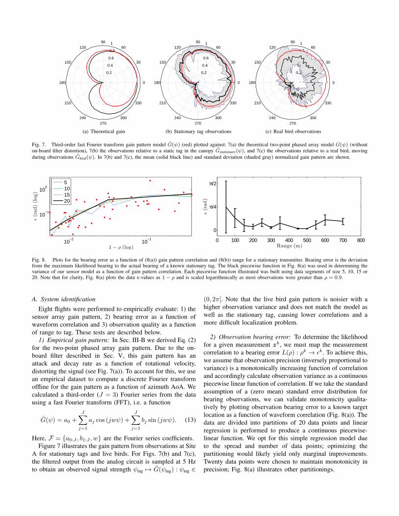
Fig. 7. Third-order fast Fourier transform gain pattern model G(ψ) (red) plotted against: 7(a) the theoretical two-point phased array model G(ψ) (withouton-board filter distortion), 7(b) the observations relative to a static tag in the canopy Gstationary(ψ), and 7(c) the observations relative to a real bird, movingduring observations Gbird(ψ). In 7(b) and 7(c), the mean (solid black line) and standard deviation (shaded gray) normalized gain pattern are shown.

10−2

10−1

10−1

100

1 − ρ (log)

ε(rad)(log)

5101520

Range (m)

ε(rad)

Range vs. Bearing Error

0 100 200 300 400 500 600 700 800

0

π/4

π/2

Fig. 8. Plots for the bearing error as a function of (8(a)) gain pattern correlation and (8(b)) range for a stationary transmitter. Bearing error is the deviationfrom the maximum likelihood bearing to the actual bearing of a known stationary tag. The black piecewise function in Fig. 8(a) was used in determining thevariance of our sensor model as a function of gain pattern correlation. Each piecewise function illustrated was built using data segments of size 5, 10, 15 or20. Note that for clarity, Fig. 8(a) plots the data x-values as 1− ρ and is scaled logarithmically as most observations were greater than ρ = 0.9.

A. System identification

Eight flights were performed to empirically evaluate: 1) thesensor array gain pattern, 2) bearing error as a function ofwaveform correlation and 3) observation quality as a functionof range to tag. These tests are described below.

1) Empirical gain pattern: In Sec. III-B we derived Eq. (2)for the two-point phased array gain pattern. Due to the on-board filter described in Sec. V, this gain pattern has anattack and decay rate as a function of rotational velocity,distorting the signal (see Fig. 7(a)). To account for this, we usean empirical dataset to compute a discrete Fourier transformoffline for the gain pattern as a function of azimuth AoA. Wecalculated a third-order (J = 3) Fourier series from the datausing a fast Fourier transform (FFT), i.e. a function

G(ψ) = a0 +

J∑j=1

aj cos (jwψ) +

J∑j=1

bj sin (jwψ). (13)

Here, F = {a0:J , b1:J , w} are the Fourier series coefficients.Figure 7 illustrates the gain pattern from observations at Site

A for stationary tags and live birds. For Figs. 7(b) and 7(c),the filtered output from the analog circuit is sampled at 5 Hzto obtain an observed signal strength ψtag 7→ G(ψtag) : ψtag ∈

(0, 2π]. Note that the live bird gain pattern is noisier with ahigher observation variance and does not match the model aswell as the stationary tag, causing lower correlations and amore difficult localization problem.

2) Observation bearing error: To determine the likelihoodfor a given measurement zk, we must map the measurementcorrelation to a bearing error L(ρ) : ρk → εk. To achieve this,we assume that observation precision (inversely proportional tovariance) is a monotonically increasing function of correlationand accordingly calculate observation variance as a continuouspiecewise linear function of correlation. If we take the standardassumption of a (zero mean) standard error distribution forbearing observations, we can validate monotonicity qualita-tively by plotting observation bearing error to a known targetlocation as a function of waveform correlation (Fig. 8(a)). Thedata are divided into partitions of 20 data points and linearregression is performed to produce a continuous piecewise-linear function. We opt for this simple regression model dueto the spread and number of data points; optimizing thepartitioning would likely yield only marginal improvements.Twenty data points were chosen to maintain monotonicity inprecision; Fig. 8(a) illustrates other partitionings.

TABLE ILOCALIZATION METRICS FOR A STATIONARY TAG. EACH TAG WAS PLACED IN THE CANOPY OF A SITE WITHIN A TARGET BIRD’S TERRITORY.

Site Trials TotalObservations

MeanError∗

(m)

MeanEntropy∗

(bits)

Mean Distance (m) Correlation ρ† Observation Error ε (rad.)†

µ (σ) µ (σ) µ (σ)

A 2 11 16.43 10.56 73.3 (22.0) 0.951 (0.0489) 0.1173 (0.0703)

B 2 11 25.2 15.7 203 (95.4) 0.941 (0.0355) 0.0691 (0.0537)

C 2 8 29.9 15.86 230 (118.9) 0.848 (0.175) 0.215 (0.349)

6 30 23.8 14.04 168.8 (78.77) 0.913 (0.0865) 0.1338 (0.1577)∗ Based on ground truth coordinate at the end of each trial† Each observation is independent of parent trial

(a) k = 1 (b) k = 2 (c) k = 6

Fig. 9. Localization of a static radio tag in a tree canopy. Figures 9(a), 9(b) and 9(c) illustrate the convergence of the a posteriori belief P(ξk|z1:k) of thetag location after the first, second and last observation for this trial, respectively. The belief is represented as a grid with 1m resolution.

(a) k = 1 (b) k = 2 (c) k = 7

Fig. 10. Localization of the Manorina Melanocephala avian species tagged with a low-power radio transmitter. Figures 10(a), 10(b) and 10(c) illustrate theconvergence of the a posteriori belief of the bird location after the first, second and last observation for this trial, respectively. As an indication of the actualbird position, the trajectory of the trackers during an observation (solid light green), and past trajectory (solid dark green) are shown.

3) System range: Figure 8(b) indicates the ideal range ofthe system as a function of bearing error. To determine theapproximate range of the system, we took various observationsat iteratively increasing distances from the tag at 50m altitudeover a flat and uncluttered environment. Figure 8(b) graphsthis range as a function of observation bearing error andqualitatively suggests the ideal system range is 100-500m.Observations closer than 100m have a high incidence elevationand thus azimuth gain is not as pronounced; observations

beyond 500m have a signal strength below the receiver’ssensitivity. Closer observations could be taken at a loweraltitude however considering time constraints per trial, uncer-tainty about target location and canopy height, it is justified tokeep a consistent height. Additionally, a higher altitude shouldincrease the received signal strength according to the two-raymodel, yet this was not observed in practice due to the inherentstochasticity in any low altitude RF application.

B. Algorithm validation: stationary tag

Six flights were performed to evaluate localization per-formance on a stationary tag in a 1000x1000m grid with1m-resolution cell edges. Table I presents the mean numberof observations per trial, mean estimation error and meanentropy of the a posteriori belief of each trial, mean andvariance of each observation range to tag, mean and varianceof observation bearing error, and the mean and variance ofthe maximum likelihood correlation of each observation. Theformer metrics report on the final observation (k = kmax)of each trial; the latter are calculated over all observationsat each site (e.g., 11 observations at Site A). Lower valuesfor all statistical metrics imply higher accuracy, precisionand certainty of the tag’s position. The observation range isdependent only on environmental factors.

Site A yields better results across all metrics, even thoughmany observations are closer than the ideal system range,most likely suggesting the actual system range is shorter thanthe free-space case presented in Sec. VI-A. Further, the site’slandscape was relatively flat with sparser vegetation than othersites and thus yields less dominant multipath propagation.In Sites B and C the algorithm performs sufficiently andconsistently localizes the stationary tag to within 30m.

A typical trial for the stationary tag at Site A is depicted inFig. 9 showing the a posteriori belief, vehicle trajectory andtag location for observations 1, 2 and 6. Ideally, the plannerwould be able to circle around the centroid, however due tosafety precautions the planner considers waypoints within a90m radius of the UAV home position (the map origin). Toaccount for the aforementioned ideal range, the planning setexcludes waypoints within 60m of the a priori belief centroid.

C. Field experiments: radio-tagged avian species

Following the algorithm validation, we performed threeflights from different launch sites to localize small, live birds.Each bird was fitted with a radio transmitter equivalent to thestationary case above. The unique frequency of each radio tagwas pre-programmed as a channel in the LMR1 receiver. Priorto each trial, a ground-based human tracker manually locatedthe bird and then recorded its position during the trial.

We present an illustration of a trial at Site A in Fig. 10.Figure 10(a) shows the launch position at approximately 300mfrom the bird in a clearing to allow direct line of sight (LoS)to the UAV system when flying toward the bird. Power lines inthe area restrict the planning distance to 90m from the home(launch) position, indicated by the 90m radius arc in Fig. 10(c).Finally, Fig. 10 shows the belief converging to a MAP estimatewithin 50m of the bird – the entropy and accuracy of this trialshould improve if the UAV could plan a larger radius aroundthe bird (see stationary tag results in Tab. I).

Results for the second and third trials are similar. Theseresults are less exhaustive and quantitative than those withstationary tags due to two reasons: 1) the inaccuracy of themanual tracking and unpredictable movement of the bird, i.e.,if a bird moves between the fourth and fifth observation themanual tracks will be lagged and 2) if the bird moves during

an observation, the observation gives the incorrect gain pattern.Further, the planning must take into account the environment(e.g., power lines) and allow an unobstructed LoS to the UAVsystem for safety precautions, causing difficulty in observingthe tag from optimal bearings.

VII. LESSONS LEARNED

Field testing revealed several interesting lessons regardingantenna performance, transmitter attenuation with live animals,and practical operation. We report these points in this section.

Our two-point phased array antenna significantly outper-forms standard H-shaped antennas typically used in UAVapplications. Although a full rotation is needed, the resultinghigh-quality bearing estimate allows for better localisationaccuracy than has been achieved with directional antennasoffline in similar applications [16]. We also found that oursystem achieved a detection range that is similar to hand-heldsystems due to the elevation of the UAV.

We expected significant signal attenuation when movingfrom the static tag to the live bird case. However, we foundsuch attenuation to be reasonable (Fig. 7). We expect that oursystem would perform well with other species of similar size.Nocturnal animals which are relatively stationary during theday are good candidates.

One limiting practical factor is short UAV flight time. Weoperated flights in quick succession by swapping batteries, butlonger duration flight would benefit localisation by allowingmore observations per flight. Advances in platforms and bat-tery energy density should mediate this issue in future.

VIII. DISCUSSION AND FUTURE WORK

We presented a full UAV system for localizing radio-taggedwildlife and demonstrated autonomous flight. Estimation isbased on a Fourier series model of expected RSSI obser-vations trained from data collected in a representative out-door environment and experimentally validated on ManorinaMelanocephala. Our future aim is to continue evaluating thissystem in field trials with different species. In our experimentsso far, we assumed that the radio tag is initially observable.In future work it is important to consider the case whereno tag is initially observable, which introduces a search anddetect component to the problem, and the issue of when theoperator should move [2], in addition to localization. It is alsoimportant to explore properties such as submodularity [17] ofthe objective function (Eq. (12)) and algorithms that exploitthese properties to maximise information while consideringtravel cost.

ACKNOWLEDGEMENTS

This work was supported in part by the Australian ResearchCouncil’s Linkage Projects funding scheme (project numberLP120100448), the Australian Centre for Field Robotics andthe New South Wales State Government. Special thanks toJeremy Randle for expert assistance with flight trials.

REFERENCES

[1] M. S. Arulampalam, S. Maskell, and N. Gordon. A tuto-rial on particle filters for online nonlinear/non-GaussianBayesian tracking. IEEE Trans. Signal Process., 50(2):174–188, 2002.

[2] G. Best, W. Martens, and R. Fitch. A spatiotemporaloptimal stopping problem for mission monitoring withstationary viewpoints. In Proc. of RSS, 2015.

[3] E. S. Bridge, K. Thorup, M. S. Bowlin, P. B. Chilson,R. H. Diehl, R. W. Fleron, P. Hartl, K. Roland, J. F. Kelly,W. D. Robinson, and M. Wikelski. Technology on themove: recent and forthcoming innovations for trackingmigratory birds. BioSci., 61(9):689–698, 2011.

[4] G. Brooker. Introduction to sensors for ranging andimaging. SciTech Publishing, Inc., 2009.

[5] F. Caballero, L. Merino, I. Maza, and A. Ollero. Aparticle filtering method for wireless sensor networklocalization with an aerial robot beacon. In Proc. of IEEEICRA, pages 596–601, 2008.

[6] Y. T. Chan, B. J. Lee, R. Inkol, and Q. Yuan. Direc-tion finding with a four-element Adcock-Butler matrixantenna array. IEEE Trans. Aerosp. Electron. Syst., 37(4):1155–1162, 2001.

[7] E. W. Frew. Observer trajectory generation for target-motion estimation using monocular vision. Phd thesis,Stanford University, 2003.

[8] S. K. Gan, R. Fitch, and S. Sukkarieh. Online de-centralized information gathering with spatial-temporalconstraints. Auton. Robot., 37(1):1–25, 2014.

[9] B. Grocholsky. Information-theoretic control of multiplesensor platforms. PhD thesis, The University of Sydney,2002.

[10] G. M. Hoffmann and C. J. Tomlin. Mobile sensornetwork control using mutual information methods andparticle filters. In Proc. of IEEE AC, pages 32–47, 2010.

[11] G. Hollinger and G. Sukhatme. Sampling-based roboticinformation gathering algorithms. Int. J. Rob. Res., 33(9):1271–1287, 2014.

[12] J. Vander Hook, P. Tokekar, and V. Isler. Cautious greedystrategy for bearing-only active localization: analysis andfield experiments. J. Field Robot., 31(2):296–318, 2014.

[13] A. M. Jensen, D. K. Geller, and Y. Q. Chen. MonteCarlo simulation analysis of tagged fish radio trackingperformance by swarming unmanned aerial vehicles infractional order potential fields. J. Intell. Robot. Syst., 74(1-2):287–307, 2014.

[14] R. E. Kenward. A manual for wildlife radio tagging.Academic Press, London, 2001.

[15] A. T. Klesh, P. T. Kabamba, and A. R. Girard. Path plan-ning for cooperative time-optimal information collection.In Proc. of IEEE AC, pages 1991–1996, 2008.

[16] F. Korner, R. Speck, A. H. Goktogan, and S. Sukkarieh.

Autonomous airborne wildlife tracking using radio signalstrength. In Proc. of IEEE/RSJ IROS, pages 107–112,2010.

[17] A. Krause and C. Guestrin. Submodularity and itsapplications in optimized information gathering. ACMTrans. Intell. Syst. Technol., 2(4):32:1–32:20, 2011.

[18] R. X. Li and V. P. Jilkov. Survey of maneuvering targettracking. Part III: Measurement models. In Proc. of SPIESDPST, pages 423–446, 2001.

[19] R. X. Li and V. P. Jilkov. Survey of maneuvering targettracking. Part I: Dynamic models. IEEE Trans. Aerosp.Electron. Syst., 39(4):1333–1364, 2003.

[20] R. X. Li and V. P. Jilkov. Survey of maneuvering targettracking. Part V: Multiple-model methods. IEEE Trans.Aerosp. Electron. Syst., 41(4):1255–1321, 2005.

[21] J. Nguyen, N. Lawrance, R. Fitch, and S. Sukkarieh.Energy-constrained motion planning for informationgathering with autonomous aerial soaring. In Proc. ofIEEE ICRA, pages 3825–3831, 2013.

[22] A. Posch and S. Sukkarieh. UAV based search for aradio tagged animal using particle filters. In Proc. ofARAA ACRA, pages 107–112, 2009.

[23] M. Quigley, K. Conley, B. P. Gerkey, J. Faust, T. Foote,J. Leibs, R. Wheeler, and A. Y. Ng. ROS: an open-source robot operating system. In Proc. of IEEE ICRA,Workshop on Open Source Software, 2009.

[24] A. Ryan and J. K. Hedrick. Particle filter basedinformation-theoretic active sensing. Robot. Auton. Syst.,58(5):574–584, 2010.

[25] P. Skoglar, J. Nygards, and M. Ulvklo. Concurrent pathand sensor planning for a UAV – towards an informationbased approach incorporating models of environment andsensor. In Proc. of IEEE/RSJ IROS, pages 2436–2442,2006.

[26] P. Soriano, F. Caballero, and A. Ollero. RF-based particlefilter localization for wildlife tracking by using an UAV.In Proc. of IEEE ISR, pages 239–244, 2009.

[27] J. Tisdale, Z. Kim, and J. Hedrick. Autonomous UAVpath planning and estimation. IEEE Robot. Autom. Mag.,16(2):35–42, 2009.

[28] P. Tokekar, D. Bhadauria, A. Studenski, and V. Isler. Arobotic system for monitoring carp in Minnesota lakes.J. Field Robot., 27(6):779–789, 2010.

[29] N. Wagle and E. Frew. Spatio-temporal characterizationof airborne radio frequency environments. In Proc. ofIEEE GLOBECOM Workshops, pages 1269–1273, 2011.

[30] C. Yoo, R. Fitch, and S. Sukkarieh. Probabilistic tem-poral logic for motion planning with resource thresholdconstraints. In Proc. of RSS, 2012.

[31] C. Yoo, R. Fitch, and S. Sukkarieh. Online task planningand control for aerial robots with fuel constraints inwinds. In Proc. of WAFR, 2014.