online learning for automatic segmentation of 3d data
TRANSCRIPT

Online learning for automatic segmentation of 3D data
Federico Tombari, Luigi Di Stefano, Simone Giardino
Abstract— We propose a method to perform automatic seg-mentation of 3D scenes based on a standard classifier, whoselearning model is continuously improved by means of newsamples, and a grouping stage, that enforces local consistencyamong classified labels. The new samples are automaticallydelivered to the system by a feedback loop based on a featureselection approach that exploits the outcome of the groupingstage. By experimental results on several datasets we demon-strate that the proposed online learning paradigm is effective inincreasing the accuracy of the whole 3D segmentation thanksto the improvement of the learning model of the classifier bymeans of newly acquired, unsupervised data.
I. INTRODUCTION AND PREVIOUS WORK
Fostered by the increasing availability of accurate andlow-cost 3D sensors, a relevant research topic within thecomputer vision and robotic communities consists in analysisof 3D data. Nowadays, many 3D sensors, based on differ-ent techniques (e.g. laser scanners, Time-of-Flight cameras,stereo cameras, ..) are able to compute range maps at avery high frame-rate. In this paper, we address the taskof automatically segmenting the sensed 3D data withina pre-defined set of objects or object categories. Such atask, usually referred to as semantic segmentation, has beensignificantly investigated over the past decade in the caseof 2D images, whilst it represents quite novel an issue asregards 3D data, with a few very recent methods proposed inliterature [1]–[4]. In fact, so far algorithms related to 3D dataanalysis have been mostly aimed at computing similaritiesbetween surfaces (e.g. [5]–[7]), while segmentation of 3Ddata among objects or object categories is currently regardedas a particularly challenging open issue, for it requires theability of handling previously unseen shapes and/or viewsand to assign correct labels to each region of the scene underanalysis.
3D data segmentation is usually dealt with by a machinelearning approach, i.e. a classifier is first trained off-line ina supervised manner to learn the distinctive shape charac-teristics of each object or object class, then it is employedon-line to classify the points belonging to the scene that hasto be segmented. This approach is motivated by the factthat the generalization ability of common classifiers holdsthe potential to deal with object deformations, previouslyunseen vantage points of a given objects as well as withthe intra-class variance of each object category. In addition,
F. Tombari is with DEIS, University of Bologna, Bologna, [email protected]
L. Di Stefano is with DEIS, University of Bologna, Bologna, [email protected]
S. Giardino is with DEIS, University of Bologna, Bologna, [email protected]
Fig. 1. Some classified feature labels (left) are modified after applying localconsistency by a MRF (right): can some of these modified labels (indicatedby a black dot) deployed to improve segmentation of forthcoming data ?
the most recent literature proposals have also tried to ex-ploit the statistical dependence among labels associated toneighboring points, so as to deploy the reasonable practicalassumption that neighboring points share always the samelabel except at object boundaries. This approach requiresthe use of specific classification techniques usually referredto as collective classification. State-of-the-art classificationapproaches used for segmentation of 3D data [1]–[3], [8]–[10] rely on Associative Markov Networks (AMNs) [11],a variant of the popular discriminative Conditional RandomField (CRF) model. These approaches achieved good perfor-mance in automatic segmentation of generic object classesfor outdoor and indoor Lidar data, although a main limitationis that the AMN formulation solves a linear classificationproblem, hence can hardly deal with articulated shapes orlarge intra-class variations.
In a different approach [12], standard local classifiers arefirst employed to perform a rough classification, successivelya grouping stage is applied, that enforces local consistencybetween classified labels through a Markov Random Field(MRF) formulation over a graph built around the classifiedfeatures. This approach has the benefit to handle any general-purpose classification technique, hence can be used withnon-linear classifiers or with kernels specifically designedto match the data characteristics. The results reported in[12] show that this method is effective with popular localclassifiers (Boost, SVM, kNN) on datasets characterizedby highly articulated shapes. Also, in [12] it is shownthat this method can effectively deal with multiple cuessimultaneously, such as color and 3D shape.
2011 IEEE/RSJ International Conference onIntelligent Robots and SystemsSeptember 25-30, 2011. San Francisco, CA, USA
978-1-61284-456-5/11/$26.00 ©2011 IEEE 4857
CLASSIFICATION GROUPING(LOCAL CONSISTENCY)
FINAL SEGMENTATION
FEATURE SELECTIONRETRAINING
3D DATA(FEATURES)
ONLINE LEARNING
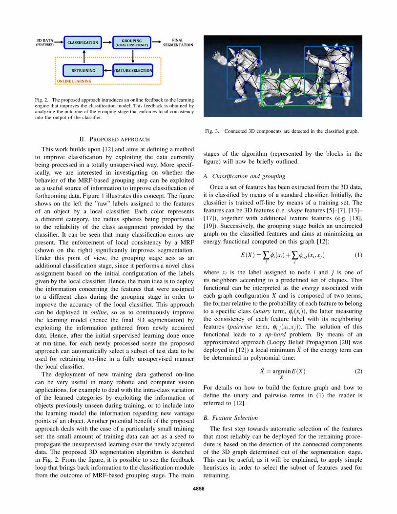
Fig. 2. The proposed approach introduces an online feedback to the learningengine that improves the classification model. This feedback is obtained byanalyzing the outcome of the grouping stage that enforces local consistencyinto the output of the classifier.
II. PROPOSED APPROACH
This work builds upon [12] and aims at defining a methodto improve classification by exploiting the data currentlybeing processed in a totally unsupervised way. More specif-ically, we are interested in investigating on whether thebehavior of the MRF-based grouping step can be exploitedas a useful source of information to improve classification offorthcoming data. Figure 1 illustrates this concept. The figureshows on the left the ”raw” labels assigned to the featuresof an object by a local classifier. Each color representsa different category, the radius spheres being proportionalto the reliability of the class assignment provided by theclassifier. It can be seen that many classification errors arepresent. The enforcement of local consistency by a MRF(shown on the right) significantly improves segmentation.Under this point of view, the grouping stage acts as anadditional classification stage, since it performs a novel classassignment based on the initial configuration of the labelsgiven by the local classifier. Hence, the main idea is to deploythe information concerning the features that were assignedto a different class during the grouping stage in order toimprove the accuracy of the local classifier. This approachcan be deployed in online, so as to continuously improvethe learning model (hence the final 3D segmentation) byexploiting the information gathered from newly acquireddata. Hence, after the initial supervised learning done onceat run-time, for each newly processed scene the proposedapproach can automatically select a subset of test data to beused for retraining on-line in a fully unsupervised mannerthe local classifier.
The deployment of new training data gathered on-linecan be very useful in many robotic and computer visionapplications, for example to deal with the intra-class variationof the learned categories by exploiting the information ofobjects previously unseen during training, or to include intothe learning model the information regarding new vantagepoints of an object. Another potential benefit of the proposedapproach deals with the case of a particularly small trainingset: the small amount of training data can act as a seed topropagate the unsupervised learning over the newly acquireddata. The proposed 3D segmentation algorithm is sketchedin Fig. 2. From the figure, it is possible to see the feedbackloop that brings back information to the classification modulefrom the outcome of MRF-based grouping stage. The main
Fig. 3. Connected 3D components are detected in the classified graph.
stages of the algorithm (represented by the blocks in thefigure) will now be briefly outlined.
A. Classification and grouping
Once a set of features has been extracted from the 3D data,it is classified by means of a standard classifier. Initially, theclassifier is trained off-line by means of a training set. Thefeatures can be 3D features (i.e. shape features [5]–[7], [13]–[17]), together with additional texture features (e.g. [18],[19]). Successively, the grouping stage builds an undirectedgraph on the classified features and aims at minimizing anenergy functional computed on this graph [12]:
E(X) = ∑i
φi(xi)+∑i
φi, j(xi,x j) (1)
where xi is the label assigned to node i and j is one ofits neighbors according to a predefined set of cliques. Thisfunctional can be interpreted as the energy associated witheach graph configuration X and is composed of two terms,the former relative to the probability of each feature to belongto a specific class (unary term, φi(xi)), the latter measuringthe consistency of each feature label with its neighboringfeatures (pairwise term, φi, j(xi,x j)). The solution of thisfunctional leads to a np-hard problem. By means of anapproximated approach (Loopy Belief Propagation [20] wasdeployed in [12]) a local minimum X of the energy term canbe determined in polynomial time:
X = argminX
E(X) (2)
For details on how to build the feature graph and how todefine the unary and pairwise terms in (1) the reader isreferred to [12].
B. Feature Selection
The first step towards automatic selection of the featuresthat most reliably can be deployed for the retraining proce-dure is based on the detection of the connected componentsof the 3D graph determined out of the segmentation stage.This can be useful, as it will be explained, to apply simpleheuristics in order to select the subset of features used forretraining.
4858

99.6100.0
91.4
80.5
69.7
99.7 100.0
91.5
80.6
70.6
0.0
10.0
20.0
30.0
40.0
50.0
60.0
70.0
80.0
90.0
100.0
Stanford Watertight-2 Watertight-4 Watertight-8 Kinect
Tru
e P
osi
tiv
es
(%)
NN
Add Add&Remove
99.795.9
89.6 86.9
64.6
99.795.9
89.5 87.0
65.6
0.0
10.0
20.0
30.0
40.0
50.0
60.0
70.0
80.0
90.0
100.0
Stanford Watertight-2 Watertight-4 Watertight-8 Kinect
Tru
e P
osi
tiv
es
(%)
SVM
Fig. 4. The % of correctly chosen features yielded the proposed feature selection stage on the experimental datasets used in Section III and relatively totwo different classifiers (SVM and NN).
To detect connected components in the scene we use thebreadth-first search algorithm (BFS) [21], an efficient graph-search algorithm that detects a connected component startingfrom a seed node and iteratively exploring all the neighboringnodes. The first step of this algorithm consists in cuttingall edges that connect two nodes having different labels.Once this is done, starting from any node we add all itsneighbors to a First-In First-Out (FIFO) queue and markthem as examined. For all the points in the queue we repeatthis procedure adding only the neighbors that have not beenexamined yet. Once the queue is empty, all the examinedpoints will be included into the same connected componentof the graph. To find the other connected components, thealgorithm is repeated again, starting from a node that has notbeen examined yet. An example of the outcome of this stageis depicted in Fig. 3, where the the connected componentalgorithm is applied over a scene of one dataset used insection III.
Once the connected components have been found, wehave to determine which nodes should be used for retrainingamong those whose class assignment was modified by thegrouping stage. The two main heuristics deployed at thisstep are: i) nodes belonging to small connected componentsare discarded, since could be easily affected by noise andwould hardly represent the surface of a whole object; ii)nodes too close to the border of the connected component arediscarded, to avoid the typical boundary effects due to clutter.To enforce these two heuristics, we simply evaluate for eachnode: i) the minimum number of nodes of its connectedcomponent (in all our experiments, it is set to one fiftiethof the total number of nodes of the graph); ii) a minimumdistance to the closest connected bordering node (in all ourexperiments, it is set to 1.5 the average distance among thenodes of the graph).
By enforcing these two simple conditions, we are ableto determine reliable points that can be provided to there-training stage. By continuously gathering new samplesfor the classifier, we incur into the disadvantage that the
training set is continuously incremented with new trainingfeatures. While this has a marginal significance with certainclassifiers such as SVM [22], where the addition of noveltraining features only changes the number and value of thesupport vectors, it can be more noticeable on others suchas kNN [2], where all training features must be stored inmemory and evaluated during the classification stage. In sucha case, the addition of novel training features would tendto continuously increase memory occupancy as well as thecomputation time to search for the best k candidates.
For this reason, we have evaluated a removal procedure,dual to that aimed at selecting novel training samples, so asto automatically select a subset of features to be removedfrom the training set. The main idea is that features reli-ably detected as ”mis-classified” could be discarded fromthe training set. More specifically, this procedure searches,for each sample selected for retraining, the most similartraining sample of the misclassified category. If the simi-larity is higher than a pre-defined threshold, this sample ispermanently discarded from the training set. This removalprocedure only affects that subset of the training set that wasadded during the online stage in an unsupervised way, since,in principle, the initial supervised set should be consideredreliable. Since applied to all samples used for re-training,this procedure allows us to discard, on the average, the samenumber of training samples as those added to the trainingset.
Although simple, the heuristics exploited for the featureselection stage are effective in selecting good candidatesfor the online learning stage. This is vouched by the chartsin Figure 4, which evaluate the performance of the featureselection stage by reporting the number of correctly chosenfeatures (True Positives, TP). In other words, since this stagecan be seen as a binary classification problem, based onexperiments with hand-labeled ground-truth it is possibleto compute the number of features that were correctlypicked up for retraining (i.e. misclassified by the classifier,correctly classified by the MRF and subsequently selected
4859

Fig. 5. Snapshots of scenes included in the considered datasets.
for retraining by the feature selection stage).More specifically, the Figure shows TPs for two different
classifiers (SVM and NN), each chart reporting the resultsyielded by the feature selection stage in the version that onlyadds retraining samples (referred to as Add, in red) as wellas in the version that carries out also the removal procedure(referred to as Add&Remove, in green), on the 5 datasetsthat will be used in the experimental Section (see SectionIII). Since the charts only take into account those points thatwere selected by the algorithm, False Positives are not shownas they would simply be equal to 1−T P. From the Figure, itis evident that the great majority of the selected features arecorrectly chosen over all datasets. Also, it is interesting tonote that the performance of the Add and of the Add&Removeapproaches are almost equivalent on all datasets.
C. Retraining
Once a reliable set of features is selected for retraining, itis added to the old training set and used for a new supervisedtraining stage of the classifier. To this purpose, although notdeployed yet in our experiments, specific online learningtechniques could be usefully deployed to render the overallapproach more computationally efficient. For example, in thecase of SVM [22] classifiers, the LASVM [23] algorithmmay be deployed to rapidly add the new features as trainingsamples for the classifier.
III. EXPERIMENTAL EVALUATION
In this section we present experimental results aimedat evaluating the effectiveness of the proposed approachfor automatic segmentation of 3D scenes. We compare theproposed online learning approach to the original method(i.e. that proposed in [12]) on several 3D datasets, which
are now briefly introduced. As done in [12], to extract 3Dfeatures from the training set and test set we have usedthe 3D feature detector proposed in [7]. The only exceptionconcerns dataset Kinect (see next subsection), since due tothe large variation in size of the models belonging to thevarious classes the difference in the number of featuresextracted from the various classes by [7] tends to bias theclassification towards bigger-sized categories: hence, withKinect, a random sampling of feature points was used (asproposed e.g. in [6]). The extracted 3D features are thendescribed by means of the well-known Spin Image descriptor[6]. The parameter values deployed for feature detection anddescription are reported in [12].
A. Datasets
The performance of the proposed segmentation algorithmis evaluated over several datasets. The first, referred to asStanford, was already used for the experimental evaluationin [12]. The training set consists of 6 full-3D models (”Ar-madillo”, ”Asian Dragon”, ”Thai Statue”, ”Bunny”, ”HappyBuddha”, ”Dragon”) taken from the Stanford 3D ScanningRepository 1, while the test and validation sets consistsof 36 ”2.5D” scenes which were obtained by renderingrandomly chosen views of 6 ”full 3D” scenes obtained byrandom rotations and translations of the models composingthe training sets. In particular, out of these 36 scenes, 6 areselected for validation and 30 for testing. This is the onlydataset that includes a validation set, since all parameters ofthe algorithms have been tuned on this dataset and then keptconstant throughout the remaining experiments. This seemsreasonable due to the purpose of our experimental evaluation:
1http://graphics.stanford.edu/data/3Dscanrep
4860

NN
SVM
22.2
9.3
14.0
39.7
63.5
17.0
5.8
10.7
35.5
53.6
17.3
5.9
10.6
35.4
52.7
0
10
20
30
40
50
60
70
Stanford Watertight-2 Watertight-4 Watertight-8 Kinect
Err
or
(%)
After classification
(intermediate result)
No Retraining
Retraining (Add)
Retraining (Add&Remove)
24.6
6.8
14.2
37.6
44.0
18.0
4.9
9.9
31.8
26.3
18.2
4.8
10.1
31.9
26.0
0
5
10
15
20
25
30
35
40
45
50
Stanford Watertight-2 Watertight-4 Watertight-8 Kinect
Err
or
(%)
1.2 1.8
4.4
13.8
24.0
0.8 1.8
4.1
10.9
19.1
0.81.8
4.1
10.9
18.8
0
5
10
15
20
25
30
35
40
45
50
Stanford Watertight-2 Watertight-4 Watertight-8 KinectE
rro
r (%
)
0.63.4 5.3
16.0
45.2
0.62.2
4.0
15.3
36.7
0.62.4
4.1
15.3
35.2
0
10
20
30
40
50
60
70
Stanford Watertight-2 Watertight-4 Watertight-8 Kinect
Err
or
(%)
After grouping
(final result)
Fig. 6. Results in terms of recognition error evaluating the use of the proposed online learning scheme before (left) and after (center) the grouping stage.Two different classifiers are evaluated (SVM and NN).
since we wish to assess the benefit of the proposed onlinelearning stage with respect to [12], the two methods shouldshare exactly the same parameter values.
A total of 3 other datasets were created from the modelsavailable within the Aim@Shape Watertight database2, whichoriginally contained 400 models, subdivided into 20 cate-gories of 20 models each. The usefulness of this dataset isthat, given the amount of different models per each category,the test scenes can be built using models not included inthe training set, hence the capabilities of the algorithms ingeneralizing to categorization and their robustness towardsintra-class variations can be evaluated.
The first dataset, dubbed Watertight-2, comprises only 2categories (Teddy bears and cups). Out of each category, 5”full 3D” models were used for training and the remaining15 for testing: using the approach deployed for the Stanforddataset, 6 ”3D” scenes were created and 3 random ”2.5D”views acquired for each scene, for a total of 18 test scenes.Similarly, two other datasets, dubbed Watertight- 4 andWatertight-8 were created, including respectively 4 and 8categories. The former includes 5 models of each categoryin the training set and 30 ”2.5D” scenes in the test set, whilethe latter includes 10 models of each category in the trainingset and 50 ”2.5D” scenes in the test set.
In addition, we acquired a novel dataset with the recentlyintroduced Microsoft Kinect device. This device is able toacquire depth and color data (i.e. RGB-D) in real-time.
2www.aimatshape.net
The dataset we built includes 5 (+ 1 for the background)categories of common grocery products such as packetsof biscuits, juice bottles, coffee cans and boxes of salt,of different brands and colors. The training set includes3 model views for each category, while the testing scenesare 16, including a high degree of clutter and occlusions.Thanks to the deployed device, this dataset includes bothcolor and depth (although the color cue is not exploited inthe experiments shown in this paper). Furthermore, by meansof a simple approach based on background subtraction, wewere able to automatically compute the ground truth (i.e.by assigning to each point of each scene the label of theclass it belongs to), hence also this dataset can be usedfor quantitative evaluation. This dataset is publicly availablefor quantitative evaluation of 3D segmentation algorithms byother researchers 3.
Finally, the performance of the proposed method is alsoevaluated on the recent New York City (NYC) dataset4, apublicly available dataset that includes urban data of the cityof New York acquired with a Lidar sensor. Since the datasetonly includes ”raw” 3D data, we selected 3 main semanticclasses (facades, vegetation, vehicles) and divided it into atraining and a test set composed of, respectively, 5 modelsfor each of the 3 classes and 11 scenes. Since the datasetdoes not include the ground-truth, regarding this particulardataset we can show here only qualitative results.
3www.vision.deis.unibo.it/fede/kinectDataset.html43D Urban Data Challenge, www.3dimpvt.org/challenge.php
4861

0
5
10
15
1 2 3 4 5 6 7 8 9 10 11 12 13 14 15 16 17 18
Err
or
Ra
te (
%)
No retraining Retraining (Add)
0
5
10
15
20
1 2 3 4 5 6 7 8 9 10 11 12 13 14 15 16 17 18Err
or
Ra
te (
%)
No retraining Retraining (Add)
After classification (intermediate result)
After Grouping (final result)
Scene #
Scene #
Fig. 7. The data selected for retraining allow for improving the segmentation performance throughout the dataset, both before (top) and after (bottom) theapplication of the MRF-based grouping stage. Note how, with the proposed online learning approach, the local classification performance (top) increasinglyimproves as long as more data is provided to the algorithm.
Retraining
(Add) humans cups fourlegs airplanes ants chairs teddies hands RECALL
humans 207 0 125 0 1 1 0 2 0,62
cups 0 1.500 5 4 0 31 1 7 0,97
fourlegs 29 2 695 0 20 0 2 21 0,90
airplanes 0 0 0 565 26 14 0 12 0,92
ants 0 4 52 8 548 10 1 2 0,88
chairs 3 0 0 20 50 295 14 17 0,74
teddies 1 0 2 0 1 21 846 2 0,97
hands 22 1 63 2 1 1 0 254 0,74
PRECISION 0,79 0,99 0,74 0,94 0,85 0,79 0,98 0,80
No
Retraining humans cups fourlegs airplanes ants chairs teddies hands RECALL
humans 205 0 108 0 1 1 0 21 0,61
cups 0 1.440 5 5 0 88 1 9 0,93
fourlegs 10 2 665 0 39 0 2 51 0,86
airplanes 1 0 0 536 22 39 0 19 0,87
ants 1 4 53 8 505 28 26 0 0,81
chairs 3 0 0 30 35 311 13 7 0,78
teddies 1 10 0 0 1 21 835 5 0,96
hands 16 1 68 2 0 1 0 256 0,74
PRECISION 0,86 0,99 0,74 0,92 0,84 0,64 0,95 0,70
Tru
e L
ab
els
Inferred Labels
Inferred Labels
Tru
e L
ab
els
Fig. 8. Confusion matrix for the Watertight-8 dataset yielded by thesegmentation algorithm using a SVM classifier with (top) and without(bottom) the use of the proposed online learning procedure.
Sample snapshots of the scenes included in each datasetare shown in Fig. 5.
B. Results
Fig. 6 shows the segmentation results with and withoutthe deployment of the proposed online learning paradigm.Results refer to the use of two different classifiers (i.e. NN,on the top row, and SVM, on the bottom row). Also, resultsare shown for both the local classification stage (intermediateresult, left column) and the final segmentation after MRF-
based grouping (right column). Each chart compares the clas-sification error reported by the 3D segmentation algorithmwithout online learning (blue) and with online learning, thelatter in the version that only adds retraining samples (Add,in red) as well as in the version that also exploits the removalprocedure (Add&Remove, in green).
As it can be seen, the proposed learning approach alwaysimproves the overall result on each evaluated dataset, bothin terms of the learning model adopted, which is able toimprove the accuracy in the classification of the singlefeature, and in terms of the final result yielded by thealgorithm after application of the MRF-based grouping. It isinteresting to note that the Add&Remove procedure obtainsequivalent results to those yielded by the Add approach,hence demonstrating that the samples that are selected in thisstage can be safely removed since do not help improvingthe learning model. Also, by comparing the 3 Watertightdatasets, it seems that the proposed approach is more ef-fective with the SVM classifier if the dataset includes ahigher number of categories, conversely with the NN clas-sifier the improvement is higher if the dataset comprises asmall number of classes. Finally, in terms of 3D data, theKinect dataset is the most challenging one, reporting thepoorest performance of the algorithms. This appears to bedue to the fact that it is also the noisiest sensor amongthose evaluated. Conversely, Stanford dataset, which includesbasically synthetic models, is the one leading to the mostaccurate final results.
In addition, Fig. 7 compares the recognition error yieldedby the proposed online learning method against the originalapproach in [12] on each scene of dataset Watertight-2. Fromthe figure, the behavior of the proposed online learningparadigm can be better evaluated. In particular, it can benoted that continuously deploying new samples for retrain-ing increasingly improves the segmentation, both after theclassification stage and after the grouping stage. Given theseresults, additional improvements yielded by the proposed
4862

Fig. 9. Qualitative results: some details of the scenes belonging to the datasets with ground-truth used for testing.
method are expectable over longer 3D data sequences.We can also evaluate in more detail the improvement
brought in by the proposed method by analyzing, in Fig 8,the confusion matrix yielded on dataset Watertight-8 by theproposed online learning and the original approach. For lackof space we can only show the results on one dataset, hencewe have selected that including the highest number of classesand intra-class variation. As it can be seen from the Figure,the proposed approach is able to yield improvements overalmost all categories, both in terms of Precision as well asRecall.
Finally, Fig. 9 shows some qualitative results yieldedby the two algorithms over some scenes belonging to theconsidered datasets (all except NYC, shown in Fig. 10). TheFigure shows also the ground truth. The colored spheres referto the extracted 3D features, with each color representing a
different category. From the Figure it can be noted that theproposed approach is able to yield overall a more accuratesegmentation of the 3D scenes. Fig. 10 shows qualitativeresults concerning the NYC dataset. In this case, the resultsare compared with the un-segmented scenes, due to the lackof ground-truth. The label colors are, respectively, red forfacades, green for vegetation and blue for vehicles. As itcan be seen, also in this case the proposed method allowsa notable improvement in the segmentation accuracy overseveral surfaces of the dataset.
IV. CONCLUSIONS
This paper proposed a novel online learning method tobe applied for improving segmentation of 3D scenes. Theproposed approach is particularly suited for robotic andcomputer vision applications where one wants to improve the
4863
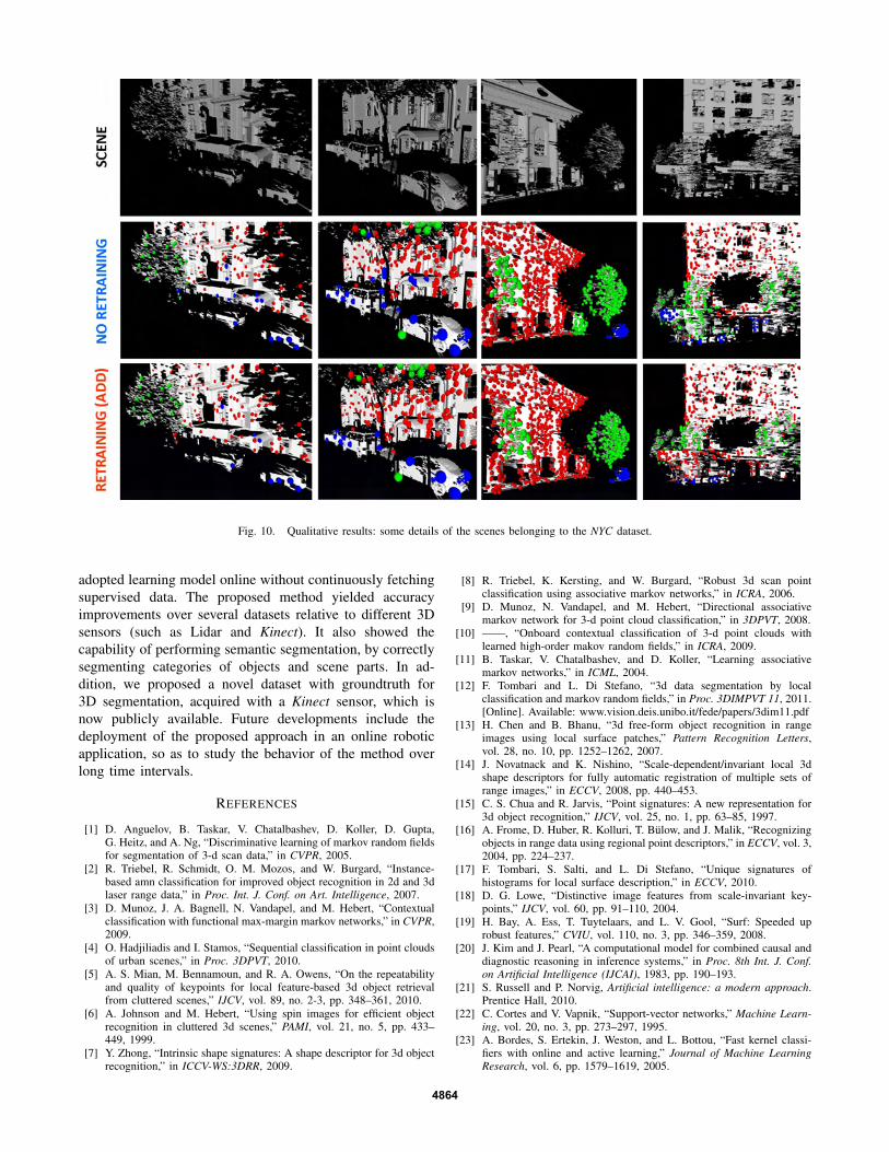
Fig. 10. Qualitative results: some details of the scenes belonging to the NYC dataset.
adopted learning model online without continuously fetchingsupervised data. The proposed method yielded accuracyimprovements over several datasets relative to different 3Dsensors (such as Lidar and Kinect). It also showed thecapability of performing semantic segmentation, by correctlysegmenting categories of objects and scene parts. In ad-dition, we proposed a novel dataset with groundtruth for3D segmentation, acquired with a Kinect sensor, which isnow publicly available. Future developments include thedeployment of the proposed approach in an online roboticapplication, so as to study the behavior of the method overlong time intervals.
REFERENCES
[1] D. Anguelov, B. Taskar, V. Chatalbashev, D. Koller, D. Gupta,G. Heitz, and A. Ng, “Discriminative learning of markov random fieldsfor segmentation of 3-d scan data,” in CVPR, 2005.
[2] R. Triebel, R. Schmidt, O. M. Mozos, and W. Burgard, “Instance-based amn classification for improved object recognition in 2d and 3dlaser range data,” in Proc. Int. J. Conf. on Art. Intelligence, 2007.
[3] D. Munoz, J. A. Bagnell, N. Vandapel, and M. Hebert, “Contextualclassification with functional max-margin markov networks,” in CVPR,2009.
[4] O. Hadjiliadis and I. Stamos, “Sequential classification in point cloudsof urban scenes,” in Proc. 3DPVT, 2010.
[5] A. S. Mian, M. Bennamoun, and R. A. Owens, “On the repeatabilityand quality of keypoints for local feature-based 3d object retrievalfrom cluttered scenes,” IJCV, vol. 89, no. 2-3, pp. 348–361, 2010.
[6] A. Johnson and M. Hebert, “Using spin images for efficient objectrecognition in cluttered 3d scenes,” PAMI, vol. 21, no. 5, pp. 433–449, 1999.
[7] Y. Zhong, “Intrinsic shape signatures: A shape descriptor for 3d objectrecognition,” in ICCV-WS:3DRR, 2009.
[8] R. Triebel, K. Kersting, and W. Burgard, “Robust 3d scan pointclassification using associative markov networks,” in ICRA, 2006.
[9] D. Munoz, N. Vandapel, and M. Hebert, “Directional associativemarkov network for 3-d point cloud classification,” in 3DPVT, 2008.
[10] ——, “Onboard contextual classification of 3-d point clouds withlearned high-order makov random fields,” in ICRA, 2009.
[11] B. Taskar, V. Chatalbashev, and D. Koller, “Learning associativemarkov networks,” in ICML, 2004.
[12] F. Tombari and L. Di Stefano, “3d data segmentation by localclassification and markov random fields,” in Proc. 3DIMPVT 11, 2011.[Online]. Available: www.vision.deis.unibo.it/fede/papers/3dim11.pdf
[13] H. Chen and B. Bhanu, “3d free-form object recognition in rangeimages using local surface patches,” Pattern Recognition Letters,vol. 28, no. 10, pp. 1252–1262, 2007.
[14] J. Novatnack and K. Nishino, “Scale-dependent/invariant local 3dshape descriptors for fully automatic registration of multiple sets ofrange images,” in ECCV, 2008, pp. 440–453.
[15] C. S. Chua and R. Jarvis, “Point signatures: A new representation for3d object recognition,” IJCV, vol. 25, no. 1, pp. 63–85, 1997.
[16] A. Frome, D. Huber, R. Kolluri, T. Bulow, and J. Malik, “Recognizingobjects in range data using regional point descriptors,” in ECCV, vol. 3,2004, pp. 224–237.
[17] F. Tombari, S. Salti, and L. Di Stefano, “Unique signatures ofhistograms for local surface description,” in ECCV, 2010.
[18] D. G. Lowe, “Distinctive image features from scale-invariant key-points,” IJCV, vol. 60, pp. 91–110, 2004.
[19] H. Bay, A. Ess, T. Tuytelaars, and L. V. Gool, “Surf: Speeded uprobust features,” CVIU, vol. 110, no. 3, pp. 346–359, 2008.
[20] J. Kim and J. Pearl, “A computational model for combined causal anddiagnostic reasoning in inference systems,” in Proc. 8th Int. J. Conf.on Artificial Intelligence (IJCAI), 1983, pp. 190–193.
[21] S. Russell and P. Norvig, Artificial intelligence: a modern approach.Prentice Hall, 2010.
[22] C. Cortes and V. Vapnik, “Support-vector networks,” Machine Learn-ing, vol. 20, no. 3, pp. 273–297, 1995.
[23] A. Bordes, S. Ertekin, J. Weston, and L. Bottou, “Fast kernel classi-fiers with online and active learning,” Journal of Machine LearningResearch, vol. 6, pp. 1579–1619, 2005.
4864