online journal of space communication applications -...

Online Journal of Space Communication Applications

Issue No. 2, Fall 2002 www.spacejournal.org of 29

A Prediction Model that Combines Rain Attenuation and Other Propagation Impairments Along Earth-

Satellite Paths

Asoka Dissanayake1, Jeremy Allnutt2, Fatim Haidara3

Abstract - The rapid growth of satellite services using higher frequency bands such as the Ka-band has highlighted a

need for estimating the combined effect of different propagation impairments. Many projected Ka-band services will

use very small terminals and, for some, rain effects may only form a relatively small part of the total propagation

link margin. It is therefore necessary to identify and predict the overall impact of every significant attenuating effect

along any given path. A procedure for predicting the combined effect of rain attenuation and several other

propagation impairments along earth-satellite paths is presented. Where accurate model exist for some phenomena,

these have been incorporated into the prediction procedure. New models were developed, however, for rain

attenuation, cloud attenuation, and low-angle fading to provide more overall accuracy, particularly at very low

elevation angles (<10°). In the absence of a detailed knowledge of the occurrence probabilities of different

impairments, an empirical approach is taken in estimating their combined effects. An evaluation of the procedure is

made using slant-path attenuation data that have been collected with simultaneous beacon and radiometer

measurements which allow a near complete account of different impairments. Results indicate that the rain

attenuation element of the model provides the best average accuracy globally between 10 and 30 GHz and that the

combined procedure gives prediction accuracies comparable to uncertainties associated with the year-to-year

variability of path attenuation.

Index Terms - Microwave radio propagation meteorological factors, Satellite communication.

I. INTRODUCTION

Rapid growth in new satellite services incorporating Very Small Aperture Terminals (VSAT) and Ultra

Small Aperture Terminals (USAT) is expected in the coming years. Small size terminals allow for widespread use

of satellite services in small business and domestic applications. Some of the services that can benefit from small

1COMSAT Laboaratories, 2300 COMSAT Drive, Clarksburg, MD 208712VPI&SU, Northern Virginia Graduate Center, 7054 Haycock Road, Falls Church, VA 22043-23113INTELSAT, 3400 International Drive, NW Washington DC 20008



earth terminals include: Internet access, multimedia applications, Local Area Network (LAN) interconnection,

Supervisory Control and Data Acquisition (SCADA) and point of sales verification. Due to congestion of lower

frequency bands such as C and Ku, most of these services will use Ka-band (20/30 GHz) frequencies. Propagation

impairments produced by the troposphere are a limiting factor for the effective use of the 20/30 GHz band and the

use of smaller earth terminals, while very attractive for customer premise location, makes it difficult to provide

sufficient link margins for propagation related outages. In this context, reliable prediction of propagation

impairments for low-margin systems becomes important. This paper reports a methodology that will allow the

prediction of different types of propagation impairments as well as combining them together to determine the

overall impact on satellite links over a wide range of outage probabilities.

Rain attenuation is the dominant propagation impairment at frequencies above about 10 GHz. In addition,

other impairments such as gaseous absorption, cloud attenuation, melting layer attenuation, and tropospheric

refractive effects becomes increasingly important with increasing operating frequency. A number of prediction

models are available for the estimation of individual components [1]-[4]. However, methodologies that attempt to

combine them in a cohesive manner are not widely available. This is partly due to the paucity of reliable measured

data required to compare and verify such approaches. The available measured data can be largely grouped into

beacon measurements and radiometric observations. In beacon measurements, the strength of a satellite-borne

beacon signal is monitored on the ground and the variations of the signal level are interpreted as propagation

impairments. However, only a relative measure of the propagation impairments can be obtained due to a lack of an

absolute calibration of the measurement system and signal variations induced by the hardware associated with the

beacon source as well as the receiving equipment on the ground. Most of the available beacon data have been

analyzed with reference to clear-sky conditions, and this process essentially removes the bulk of the low-attenuation

producing phenomena. Radiometers rely on sky noise temperature variations to estimate propagation impairments.

Although the technique provides an absolute measure of the impairment level, only absorptive phenomena due to

particulate matter and gases can be measured. In addition, there are several limitations to radiometer observations,

including restricted dynamic range and the sensitivity to thermal emissions from regions outside those that affect a

satellite link at the same look angle as the radiometer. In order to capture all propagation phenomena a combination

of beacon and radiometer measurements are normally required. Some of the more recent data collected using the



INTELSAT system [5], the European Space Agency (ESA) Olympus satellite [6], and the National Aeronautics and

Space Administration (NASA) Advanced Communications Technology Satellite (ACTS) [7] are of this type and

provide a useful database to enable the evaluation of propagation models which attempt to combine different

propagation effects.

In synthesizing an overall propagation impairment prediction procedure both existing and new models were

used for individual phenomena. Well established models exist for gaseous absorption and tropospheric

scintillations [1]. It has been reported that most of the available rain attenuation prediction models provide an

annual average accuracy of the order of 30% [8], a level which is usually not considered acceptable to satellite

system designers. The model accuracy reported in [8] is supported by recent testing efforts in the ITU-R [35]. A

lower limit to the prediction accuracy for rain attenuation models is set by the natural variability of the rain process

itself, which is thought to be around 20% on an annual basis [33].

This paper reports on an effort to devise a rain attenuation prediction procedure that provides an accuracy

comparable with the natural variability. In addition, new methodologies for predicting cloud attenuation and low-

angle fading were also developed since these phenomena become increasingly important at low elevation angles.

Descriptions of individual prediction methods used in constructing the overall model are given in Section 2. The

approach taken in combining the individual components to derive the overall attenuation distribution is presented in

Section 3. An evaluation of the model was carried out using some of the more recent slant path data that have been

collected with beacon/radiometer techniques; results of the evaluation are presented in Section 4.

II. PROPAGATION MODELS

Propagation factors considered for inclusion in the overall prediction procedure are: gaseous

absorption, cloud attenuation, melting layer attenuation, rain attenuation, tropospheric scintillations, and low-angle

fading. Low-angle fading is a refractive phenomena encountered on very low elevation angle paths (<5°) when the

propagation path passes at grazing incidence across a boundary between two air masses of different refractive index,

thereby causing focussing and defocussing of the energy as the air/air boundary moves with respect to the path [24].

Other impairments that affect satellite links in the Fixed Satellite Service (FSS) are bulk refractive effects and

ionosphere effects. These were not considered for the discussion due to the existence of standard procedures for the



prediction of bulk refractive effects[9] and the fact that the ionosphere does not produce significant signal

degradation at frequencies above about 10 GHz. Prediction procedures used for the selected components are

presented below.

A. Gaseous Absorption

A method for predicting absorption due to atmospheric gases (oxygen and water vapor) is given in ITU-R

Recommendation P.618 [1]. The input parameters required for the calculation include frequency, path elevation

angle, height above mean sea level, and the water vapor density. The calculation procedure is reproduced in Annex

I. The oxygen attenuation is considered a background effect with very little temporal variation; variations in

gaseous absorption arise from changes in the amount of water vapor in the atmosphere. In order to estimate the

distribution of gaseous absorption on an annual basis, the annual distribution of water vapor density is required. It

is generally observed that the water vapor density distribution follows the normal probability law [10]. If a

complete characterization of the distribution is not available an approximate distribution can be constructed using

the annual average water vapor density as the mean value and a quarter of that as the standard deviation.

B. Cloud Attenuation

Several models are available for the prediction of cloud attenuation [11]-[14]. An evaluation of these

models by the authors revealed that they are either poor estimators or the input data required are difficult to obtain

for a general purpose application. A comparison of different cloud models presented in [38] largely confirms this

assertion. In view of this, a cloud attenuation model based on available cloud cover data and the average properties

of different cloud types was developed. A cloud cover atlas based on daily visual observations of cloud can be

found in Reference 15. A ten year observation period has been used in constructing the maps. Cloud cover

percentages for different cloud types are given for land areas with a resolution of 5°x5° in longitude and latitude.

The data grid resolution is commensurate with the geographical distribution of the data collecting centers and this

level of resolution is deemed reasonable for the calculation of cloud attenuation. It should be noted that rain zones

[2,10] are employed in the prediction of rain attenuation and the rain zones have much larger geographical extents

compared to the 5°x5° grid used for clouds. Although cloud distributions in adjacent grids do not differ



significantly from each other, marked differences in individual cloud amounts are encountered when latitude

separation exceeds about 10°. Four cloud types were selected for the development of the cloud attenuation model,

and Table 1 summarizes the average properties of the selected cloud types derived from [39] and [40].

TABLE I

Average Properties of the Four Cloud Types Used in the Cloud Attenuation Model

Cloud Type Vertical Extent

(km)

Hc

Horizontal

Extent (km)

Lc

Water Content

(g/m3)

υ

Cumulonimbus 3.0 4.0 1.0

Cumulus 2.0 3.0 0.6

Nimbostratus 0.8 10.0 1.0

Stratus 0.6 10.0 0.4

The model was derived using the average cloud properties together with the assumption that the statistical

distribution of cloud attenuation follows the log-normal probability law. This assumption is thought to be

reasonable considering that most measured slant-path attenuation data conform to the log-normal distribution. It is

also assumed that there is no overlap between the occurrence probabilities of the four cloud types so that the

attenuation produced by each cloud type represents a distinct point in the probability distribution.

The annual cumulative contributions of cloud attenuation from the various cloud formations encountered at

different heights along a zenith path at a given location are obtained from the annual average total cloud cover,

individual cloud cover amounts for the four cloud types, their vertical dimensions, and the specific attenuation.

This provides the zenith cloud attenuation distribution, with the distribution being conditioned to the total cloud

cover.



The cloud attenuation model requires four steps as set out below.

Step 1

The specific attenuation for each of the four cloud types is obtained. These can be related to the cloud water content

using the Rayleigh approximation for small water droplets [16]:

αci = 0.4343 3πυ32λρ Im 1-ε

2+ε (dB/km) (1)

where υ - cloud liquid water content (g/m3)

λ - wavelength (m)

ρ - density of water (g/cm3)

ε - complex dielectric constant of water

Im - imaginary part of a complex number

and i is 1 to 4 for the four cloud types.

The above relationship is temperature dependent through the complex dielectric constant and the density of water.

However, the sensitivity to temperature is a second order effect and the specific attenuation calculated at 0°C is used

in the model.

Step 2

Total zenith attenuation Aci for each of the cloud types (i=1 to 4) is given by the product of the specific attenuation

and the vertical extent, namely:

Aci = 1/3 αci Hci (2)

For elevation angles other than zenith, the attenuation through each cloud type is calculated assuming the cloud

shape to be a vertical cylinder having the horizontal and vertical dimensions (Hc and Lc) shown in Table 1.

Step 3.

The four cloud types when arranged in rank order of attenuation provide four points on the conditional cloud

attenuation distribution curve, Ac, which has the following form:

P(A> Ac) =Po

2 erfc

ln A - ln A c

2 σc

(3)



where P is the probability of cloud attenuation Ac not exceeding A, Po is the probability of cloud attenuation being

present, erfc denotes the complementary error function, A c is the mean value of Ac and σc is the standard deviation

of Ac. The total cloud cover provides the conditional probability for the cloud attenuation distribution.

Step 4

With the five points selected above, the best fit log-normal relationship for the cloud attenuation distribution is

obtained using linear regression analysis.

The model is fairly simple and assumes that different parts of the cumulative cloud attenuation

distribution, Ac, are accounted for by a single cloud type. This is not strictly true since cloud properties vary

widely and the same attenuation level can be expected from more than one cloud type. In addition, different cloud

types can be present simultaneously at a variety of heights. However, the available data do not permit the

development of a model which can account for the attenuation distribution of each individual cloud type.

In order to combine the attenuation contribution of clouds into a comprehensive prediction procedure, it is

necessary to define the end-points of the cumulative distribution of path attenuation due to clouds. The minimum-

attenuation end-point will be defined by the onset of “clear-sky” conditions, when no clouds are present; the

maximum-attenuation end-point will be set at the point when light rainfall exists in the path. To obtain the

percentage-time boundary between clear-sky conditions and clouds being present, average total cloud cover data were

used: this will define the high percentage time end of the cloud attenuation distribution. To obtain the low

percentage time end of the cloud attenuation distribution, the point where rain and melting layer attenuation merge

with cloud attenuation is used. The latter point, where rain, melting layer, and cloud effects merge, is not a well

defined boundary and will depend on both the geographic location and the elevation angle. This aspect of cloud

attenuation modeling is discussed in section 3 on combining the impairments.

Examples of model predictions compared with direct estimates of cloud attenuation data are shown in

Figures 1a and 1b. Data in Fig. 1a are from Darmstadt in Germany [17] where radiometers have been used to

estimate cloud attenuation statistics for a period of 12 months. The cloud attenuation estimate for New York, NY,

shown in Fig. 1b is based on one year of surface and radiosonde observations. Percentage cloud cover amounts

used for the model predictions and the best fit log-normal distribution parameters for the two sites are shown Table

2. It is seen that in both cases good agreement between the model prediction and the direct estimate exist.



TABLE 2

Cloud Parameters for the Predicted Cloud Attenuation Distributions Shown in Figure 1

Parameter Darmstadt New York

Percentage of Cumulo Nimbus 2.0 2.3

Percentage of Cumulus 4.0 3.0

Percentage of Nimbostratus 12.0 13.5

Percentage of Stratus 37.3 34.5

Percentage of Total Cloud Cover, Po 63.3 70.5

A c 0.433 0.227

σc 0.705 0.956

C. Melting Layer Attenuation

The melting layer is the region around the 0°C isotherm where ice and snow particles from aloft melt to

form rain drops. The melting layer thickness, Dm, is of the order of 500 m and a distinct layer such as the radar

bright band exists only for relatively low rain rates [18]. Attenuation produced by the melting ice particles can

reach significant levels, especially for low-elevation angle links. The specific attenuation in the melting layer,

however, is not always significantly larger than that in the rain region underneath it. Rain attenuation modeling,

being largely semi-empirical, normally accounts for melting effects for moderate to high rainfall rates (i.e. ≥ 2

mm/h). As such, it is felt that a separate account of the layer is required only for low rain rates. Several models for

predicting melting layer effects are available [19]-[21] and the one proposed in Reference 21 was selected for its ease

of implementation. Using this model the following relationship between the rain rate, R, and the specific

attenuation in the melting layer, αm, was derived:

αm = aRb (dB/km) (4)

where

a = e1.58 ln (f) - 6.23

b = e0.029 ln(f) + 0.031

and R is the rain rate in mm/h and f is the frequency in GHz.



The width of the melting layer, Dm, is taken to be 0.5 km and the path length through the melting layer, Lm, is

taken to be Lm = 0.5sinθ (km) where θ is the elevation angle; the path length is restricted to a maximum value of 10

km. Thus, melting layer attenuation, Am, is given by:

Am = αm Lm (dB) for Lm ≤ 10 km max. (5)

D. Rain Attenuation

Rain attenuation modeling on satellite paths has been undertaken by many research groups over the last

four decades. The models generally fall into two categories: (a) those that attempt to define the physics of the

process and model the constituents of storm cells, etc., and (b) those that use empirical approaches with simplified

assumptions. Due to the lack of world-wide information on many of the physical inputs needed to provide accurate

results using the models of type (a), type (b) models - empirical procedures - have tended to be used most often and

with usually the best results. In Working Party 3M of Study Group 3, extensive testing of all of the leading rain

attenuation models has been undertaken [35] and the better formulated of the empirical models scored the highest,

one of them being the current ITU-R procedure [1].

The proposed rain attenuation prediction model is somewhat similar to the one recommended by the ITU-R

[1] where the rain related input to the model is the rain intensity at the 0.01% probability level. The method was

derived on the basis of the log-normal distribution using similarity principles [22]. Both point rain intensity and

path attenuation distributions generally conform to the log-normal distribution given by equation (3).

Inhomogeniety in rain in the horizontal and vertical directions are accounted for in the prediction. The same

procedure applies for both slant paths and terrestrial paths. The method is applicable across the frequency range 4 to

35 GHz and percentage probability range 0.001% to 10%. Input data required for the model and the step-by-step

procedure for calculating the attenuation distribution is given below.

Input data required for the model are:

• latitude of the earth station - φ (deg)

• altitude of the earth station above the mean sea level - hs (km)

• point rainfall rate for 0.01% of an average year - R0.01 (mm/hr)

• percentage exceedance probability for which attenuation is to be calculated - p



• elevation angle - θ (deg)

• frequency - f (GHz)

• polarization angle - ξ (deg)

• effective earth radius - Re = 8500 km

Step 1

Freezing height during rain, hfr (km), is calculated from the absolute value of station latitude, φ (degrees),

as:

hfr = 5.0 for 0° ≤ φ < 23°

(6)

hfr = 5.0 - 0.075 (φ - 23) for φ ≥ 23°

Step 2

The slant-path length, Ls, below the freezing height is obtained from

Ls = (hfr - hs) / sinθ (km) (7)

where θ is the elevation angle and hs is the station height in km. For elevation angles less than 5°, a more accurate

path length estimate can be made using:

Ls = 2(hfr - hs)

[sin2θ + 2(hfr -hs)

Re]1/2

+ sinθ

(km) (8)

Step 3

The horizontal projection, Lg, of the slant path length is found from:

Lg = Ls cosθ (km) (9)

Step 4

Obtain the rain intensity, R0.01(mm/hr), exceeded for 0.01% of an average year, and calculate the specific

attenuation, γ (dB/km), using widely published frequency and polarization dependent coefficients k and α [9],[31]

:

γ = k (R0.01)α (dB/km) (10)

Step 5



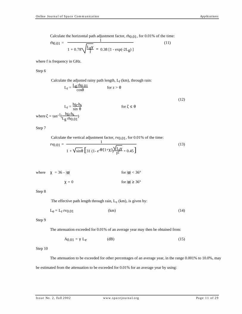
Calculate the horizontal path adjustment factor, rh0.01, for 0.01% of the time:

rh0.01 = 1

1 + 0.78Lgγ

f - 0.38 [1 - exp(-2Lg) ]

(11)

where f is frequency in GHz.

Step 6

Calculate the adjusted rainy path length, Lr (km), through rain:

Lr = Lg rh0.01

cosθ for z > θ

(12)

Lr = hfr-hssin θ for ζ ≤ θ

where ζ = tan-1(hfr-hs

Lg rh0.01)

Step 7

Calculate the vertical adjustment factor, rv0.01, for 0.01% of the time:

rv0.01 = 1

1 + sinθ [31 (1- e-θ/[1+χ])Lrγf2

- 0.45](13)

where χ = 36 - |φ | for |φ | < 36°

χ = 0 for |φ | ≥ 36°

Step 8

The effective path length through rain, Le (km), is given by:

Le = Lr rv0.01 (km) (14)

Step 9

The attenuation exceeded for 0.01% of an average year may then be obtained from:

A0.01 = γ Le (dB) (15)

Step 10

The attenuation to be exceeded for other percentages of an average year, in the range 0.001% to 10.0%, may

be estimated from the attenuation to be exceeded for 0.01% for an average year by using:



Ap = A0.01 p0.01

-[0.655 + 0.033 ln p - 0.045 ln A0.01 - z sinθ (1-p)](16)

where p is the percentage probability of interest and z is given by:

For p ≥ 1% z = 0

for p < 1%

z = 0 for |φ | ≥ 36°

z = -0.005 (|φ | - 36) for θ ≥ 25° and |φ | < 36°

z = -0.005 (|φ | - 36) + 1.8 - 4.25 sinθ for θ < 25° and |φ | < 36°

The above procedure was tested by the ITU-R and found to be the most accurate overall of all models tested [35].

E. Tropospheric Scintillations

A procedure for predicting tropospheric scintillation is given in the ITU-R Recommendation 618 [1]; this

is reproduced in Annex II. The key input parameters for the model are: frequency, elevation angle, antenna

diameter, average temperature and average relative humidity. It first calculates the standard deviation of the signal

amplitude fluctuations, σχ, from which the scintillation distribution is constructed. The model is semi-empirical

and has been found in testing by ITU-R Study Group 3 to replicate measured results very well at elevation angles

above about 4° (see, for example, [36]).

F. Low-angle Fading

In still air, the atmosphere assumes a stratified form with layers of generally decreasing refractive index

lying one above the other. Slight horizontal wind movement will cause these layers to fold, rather like the strata of

the Earth under tectonic stress, such that the boundary between layers of different refractive index can be inclined a

few degrees to the horizontal. This slight change in angle has no effect on satellite links with elevation angles well

above 10o. At elevation angles below 10

o, and particularly below 5

o, the signal path to or from the satellite may be

at grazing incidence to the tilted air/air refractive index boundary. Changes in position of the refractive index

boundary with respect to the signal path, brought about by relative movement of the atmospheric layers and the

satellite path, can lead to large changes in energy levels at the ends of the signal path. These changes are due to

large scale refractive irregularities across the layer boundary and thus have a minimal dependence on radio frequency,



unlike tropospheric scintillation which is due to small scale refractive index variations and which therefore has a

strong frequency dependence [1].

The ITU-R tropospheric scintillation model performs quite well for elevation angles down to about 5°.

Below this elevation angle, low-angle fading begins to appear in measured cumulative statistics. After an

investigation of available scintillation data for elevation angles below 5°, the ITU model was extended below 5°

elevation angles in this new approach by supplementing the tropospheric scintillation fading with additional fading

due to low-angle effects. The extension to the scintillation model in this paper modifies the ITU-R tropospheric

scintillation standard deviation,

σχ, and takes effect only at elevation angles below 5°. The modified standard deviation σt for deriving the fading

distribution is given by:

σt = σχ + σo (ea(5-θ) - 1.0 ) (0° < θ < 5°) (17)

where σo is the scintillation standard deviation at a frequency of 4 GHz and an antenna diameter of 4 m, and a is an

empirical constant equal to 0.11. The σo term accounts for low-angle fading which is essentially frequency

independent. It was derived using experimental fading data from two experiments; one in Clarksburg, MD [23],

and the other in Ottawa, Canada [24]. Both experiments used antennas with diameters close to 4 m.

Predictions made with the above equation are compared with measured results in Figure 2. The

discrepancy between the measured and the predicted fades appears to compare well with potential errors involved in

the measurements of signal scintillations and low-angle fading. It should be noted that unlike in the ITU

scintillation model, σt applies only to the fading part of the distribution. The tropospheric scintillation model [1]

has been recommended for use between 4 and 20 GHz, but recent Olympus and ACTS measurements have shown it

to be accurate in predicting scintillation effects up to about 30 GHz. The low-angle fading model presented here

included the ITU-R tropospheric scintillation model and so should be applicable up to at least 30 GHz.



III. COMBINING IMPAIRMENTS

All the propagation impairments discussed in previous sections originate in the lower troposphere and their

respective sources are highly interdependent. Some examples are: cumulus clouds can produce both attenuation and

scintillations; the melting layer is associated with low-intensity rain; and gaseous absorption increases during rain

due the increased water vapor content in the atmosphere. As a result, a procedure for combining the different

impairments to produce an overall cumulative fade distribution is not directly evident. This is compounded by the

fact that most impairment prediction models are semi-empirical in nature due to an incomplete understanding of the

physical mechanisms as well as the lack of an adequate characterization of the various sources producing the

impairments. Methodologies available for combining impairments generally limit themselves to combining only

the absorptive and non-absorptive components [1,37].

Several approaches were considered for combining the individual attenuation contributions to produce the

overall attenuation distribution. These were: direct addition on an equi-probable basis, root-sum-square addition on

an equi-probable basis, equi-probable weighted addition, and statistical interpolation. A combination of these

approaches was used for the various impairment phenomena. Two main areas of uncertainty were encountered: (1)

how to combine the individual attenuation contributions and, as fundamental, (2) how to approach the transition

region between clear-air and precipitation.

For topic (1), several approaches were considered for combining the individual contributions. These were:

direct addition on an equiprobable basis; a root-summed-squared addition on an equiprobable basis; an equiprobable

weighted addition; and statistical interpolation. A combination of these approaches was eventually used as will be

shown later in this section. For topic (2) an empirical approach to combining impairments in this region was taken

by identifying possible approaches and checking them against the measured distributions. To this end, statistical

interpolation and equi-probable weighted addition were considered. Measured data normally show that the

attenuation distribution is continuous, with no break-point between the clear-air region and the precipitation region.

On this basis it was thought appropriate to divide the absorptive part of the overall attenuation distribution into two

distinct regions, viz. clear-air and precipitation , with the region in between filled in with interpolated values. This

worked well at frequencies below 10 GHz since the attenuation produced by low precipitation levels was comparable

to those produced by clouds and a smooth transition between the clear-sky and precipitation regions resulted. Due



to the relatively low levels of attenuation expected at frequencies of less than 10 GHz, a fixed set of boundaries were

selected. These were:

• the precipitation region was defined by percent probabilities < 0.5%

• the clear-air region was defined by percent probabilities > 10%

Attenuation statistics are assumed to follow a log-normal distribution and the attenuation in the transition region

between the precipitation region and the clear-air region derived using log-normal interpolation between the

attenuation values at 0.5% and 10%.

For frequencies above 10 GHz, a different approach was found to be necessary. This combined

impairments using a weighted sum of absorptive components for probability levels between τ1% and τ2%; τ1 is a

variable dependent on the rain climate and τ2 is a function of the elevation angle. Above the τ2% level, the

impairments are entirely due to clear-air effects and below τ1% mainly rain attenuation and gaseous absorption

contribute to the absorptive component. The τ1 level is set by the upper limit of rain rate for which the melting

layer attenuation model is considered valid (i.e. R ≤ 2 mm/h). The resulting distribution for the absorptive

components can now be added to the scintillation contributions on a root-sum-squared basis [1]. The root-sum

addition between absorptive and non-absorptive components appears to produce adequate results that compare well

with measured data.

For the combination process, the following parameters are used.

Ax(p) is the attenuation exceeded for p percent of time with

At - total attenuation

Aa - absorptive component

As - refractive component

Ar - rain attenuation

Ag - gaseous absorption

Ac - cloud attenuation

Am - melting layer attenuation

Acm = Ac2 + Am2 - cloud and melting layer attenuation

Arcm - combined attenuation from rain, clouds, and melting layer



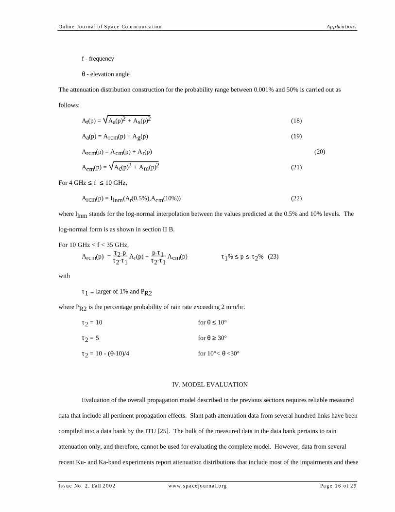
f - frequency

θ - elevation angle

The attenuation distribution construction for the probability range between 0.001% and 50% is carried out as

follows:

At(p) = Aa(p)2 + As(p)2 (18)

Aa(p) = Arcm(p) + Ag(p) (19)

Arcm(p) = Acm(p) + Ar(p) (20)

Acm(p) = Ac(p)2 + Am(p)2 (21)

For 4 GHz ≤ f ≤ 10 GHz,

Arcm(p) = Ilnm(Ar(0.5%),Acm(10%)) (22)

where Ilnm stands for the log-normal interpolation between the values predicted at the 0.5% and 10% levels. The

log-normal form is as shown in section II B.

For 10 GHz < f < 35 GHz,

Arcm(p) = τ2-pτ2-τ1

Ar(p) + p-τ1τ2-τ1

Acm(p) τ1% ≤ p ≤ τ2% (23)

with

τ1 = larger of 1% and PR2

where PR2 is the percentage probability of rain rate exceeding 2 mm/hr.

τ2 = 10 for θ ≤ 10°

τ2 = 5 for θ ≥ 30°

τ2 = 10 - (θ-10)/4 for 10°< θ <30°

IV. MODEL EVALUATION

Evaluation of the overall propagation model described in the previous sections requires reliable measured

data that include all pertinent propagation effects. Slant path attenuation data from several hundred links have been

compiled into a data bank by the ITU [25]. The bulk of the measured data in the data bank pertains to rain

attenuation only, and therefore, cannot be used for evaluating the complete model. However, data from several

recent Ku- and Ka-band experiments report attenuation distributions that include most of the impairments and these



are used for the model evaluation; Table 3 gives key parameters of the data sets used for the comparison [6], [25]-

[29].

The proposed rain attenuation model requires rain intensity, with an integration time of the order of one

minute, exceeded for 0.01% (R0.01) as the main input parameter. This parameter can be obtained from a rain model

or measured rain intensity data. Since measured rain intensity data are not generally available, recourse must be

made to a rain model; Some of the available options are:

• conversion of daily or hourly rain intensity to one minute rain intensity

• rain zone classification of the ITU-R [10]

• Crane global rain model [2]

• Rice-Holmberg rain model [30]

Rain zone models such as the ITU-R and Crane global model embody broader climatic features of widely

separated regions. As such, they tend to be rather coarse and may not always be appropriate for obtaining

site specific rain intensity data. Conversion of long integration time rain intensity to short integration

time rain rates is more direct and can be made site specific using widely available rainfall data from

meteorological stations. The Rice-Holmberg (R-H) model requires the average annual accumulation of

rainfall and the fraction of this rain arising from thunderstorm activity as input parameters. The model

provides one-minute averaged estimates of point rain rate R (mm/h) exceeded for a particular percentage of

an average year, P, using the equation:

P(r > R) = M

87.66 { 0.03β e-0.03R + 0.2 (1 - β) [e-0.258R + 1.86 e-1.63R]} (24)

where

M - average annual accumulation of rainfall (mm)

β - thunderstorm component of M given by [32]:

β = βo [0.25 + 2 e-0.35 (1 + 0.125M)/U]

βo = 0.03 + 0.97 e-5 exp(-0.004Mm)

where U is the average number of thunderstorm days expected during an average year and Mm is the highest

monthly precipitation observed in 30 consecutive years.



The required input data can be obtained from meteorological data sources and regional maps. In addition,

they are easier to manipulate than the long integration time rain intensity data. Although the R-H model has been

developed largely on the basis of rainfall measurements made in the US, it has been found to be applicable to other

parts of the world as well. In light of this, the Rice-Holmberg model was selected to obtain the R0.01 values for

the rain attenuation calculation. The M and β values for the selected experiment locations are also shown in Table

3. In addition, the Table includes the measured value of R0.01 whenever they are available. It can be seen that the

agreement between the predicted and measured R0.01 values is reasonable. However, consideration to the following

must be given when comparing the data:

• most measured rain intensity data shown in Table 3 pertain to a measurement period of one or two years.

To obtain stable statistics, a measurement period in excess of five years is usually recommended. Year-to-year

variability of rain intensity at a given site can be as much as 30%.

• the thunderstorm factor is an empirically derived parameter based on the number of average thunderstorm

days in a year and the maximum monthly rainfall. When these parameters are not available, a less accurate estimate

can be made using regional maps of β [32], [33].

The measurement sites listed in Table 3 report total attenuation in some form allowing the model to be

compared at probability levels well in excess of 1%. However, not all model components could be included for all

sites. Some sites report beacon attenuation data that have been low-pass filtered to remove scintillation effects. In

the ensuing comparison the most appropriate impairment components were used in making the predictions.

Comparisons are based on the percentage prediction error defined as:

ei = Api - Ami

Ami x 100 (25)

where Ap is the predicted attenuation and Am is the measured attenuation, both in dB, and i represents the percent

probability level at which the prediction error is estimated. The RMS error is used as the metric to judge the

overall fit of the prediction with the measurement, and is given by:

erms = <ei2> (26)

where <> denotes averaging.

The percent probability levels used for the comparison range from 10%, to 0.001% with four points in each

decade of probability (1, 2, 3, and 5). Figures 3 through 14 show comparisons between measured and predicted



attenuation distributions for sites reporting Ka-band measurements. Results of the comparison are given in Table 3.

Out of the 30 links used for the test, 18 produced RMS errors of less than 20%. The average RMS error was

19.5%. One of the links (12.5 GHz at Blacksburg) produced a rather large RMS error of 45%, mainly due to the

relatively high value of the R0.01 predicted by the R-H model in comparison with the long-term measured value.

The observation period associated with most of the links is less than two years and part of the prediction error can

be attributed to the annual variability of attenuation. In most cases the errors are comparable to the year-to-year

variability associated with path attenuation, and it can be concluded that the prediction procedure is in reasonable

agreement with the measured data. In recent testing of eleven rain attenuation prediction models [34], the modified

rain attenuation procedure proposed in this paper was found to be the best on average.

V. CONCLUSIONS

A procedure suitable for the prediction of propagation impairments along earth-satellite paths is described.

The method can be used to predict individual impairments as well as their combined effects at frequencies between 4

GHz and 35 GHz although the best accuracy will be found between 10 and 30 GHz. Based on the limited

comparisons presented in Section 4, the method appears to be able to predict total path attenuation with an overall

error of less than 20%. The method predicts the long-term average attenuation values for a given link and the

comparisons were not always made with long-term observations. The year-to-year variability of attenuation on a

given link is of the order of 20% [8] and the prediction accuracy compares well with this value.

The dominant propagation impairment at frequencies above 10 GHz is rain attenuation. The prediction of

rain attenuation requires either measured rain data or a fairly representative rain model to obtain the 0.01% rain rate.

The model comparisons presented in Section 4 were made using the Rice-Holmberg rain model and the relatively

low levels of the prediction error points to the usefulness of this rain model for propagation impairment predictions.

The proposed rain attenuation model can be used for terrestrial paths as well (i.e. for θ = 0°). This feature is

currently a requirement in the ITU-R prediction procedure for rain attenuation. Comparison of the model proposed

here with the terrestrial rain attenuation database in the ITU-R data bank [25] using measured rain intensity data

given in the data bank produced an average RMS prediction error of 23%.



Available measured data appear to validate the cloud attenuation model presented. Cloud attenuation is

limited to less than about 1.5 dB at the frequencies used for the model evaluation. The available cloud cover data

are rather coarse and a more refined model based on long-term observations of atmospheric profiles of water vapor,

pressure, and temperature may be more appropriate for the prediction of cloud attenuation at frequencies higher than

about 35 GHz. The procedure outlined in [37] may help to improve this aspect.

The melting layer can play a significant role under low elevation angle conditions. The proposed model is

applicable only when a distinct melting layer is present, such as under stratiform rains of low intensity. When a

distinct melting layer is not present the specific attenuation in the melting region appears to be comparable to that

in the rain region.

The model provides predictions across the probability range of 0.001% to 50%. This range is thought to

be adequate for most telecommunication system design purposes. Use of the model outside the specified range is

not recommended since all factors required for a complete description of the cumulative distribution are not included

in the model.



ACKNOWLEDGMENT

The work reported was carried out under INTELSAT contract INTEL-869. Any views expressed in this paper are

not necessarily those of COMSAT, INTELSAT, or the Virginia Polytechnic Institute and State University.



ANNEX I

CALCULATION OF GASEOUS ABSORPTION

Gaseous absorption is calculated as the sum of water vapor absorption and Oxygen absorption [1].

The procedure described below applies to frequencies up to 350 GHz.

The specific attenuation of water vapor, γ w (dB/km), for a ground level pressure of 1013 hPa and

a temperature of 15°C is given by:

γ w = 0.05+0.0021µ+3.6

(f-22.2)2+8.5 +

10.6(f-183.3)2+9.0

+8.9

(f-325.4)2+26.3f2µ10-4 (dB/km) (A1)

where:

f - frequency (GHz)

µ - water vapor density (g/m3)

The total attenuation due to water vapor is given by:

Aw = hwγ w/sinθ (dB) for θ >10°

(A2)

Aw = γ w Rehw

cosθ F(tanθ Re/hw ) (dB) for θ ≤ 10°

where:

Re - effective earth radius including refraction (8500 km)


F(x) = 1

0.661x + 0.339 x2 + 5.51(A3)

hw - equivalent height of water vapor given by:

hw = hwo 1 + 3

(f-22.2)2+5 +

5(f-183.3)2+6

+2.5

(f-325.4)2+4 (km) (A4)

hwo = 1.6 km (in clear weather outside the absorption regions)

The specific attenuation of oxygen, γ o (dB/km), is given by:

γ o = 7.19x10-3+ 6.09

f2+0.227 +

4.81(f - 57)2 + 1.5

f2x10-3 (A5)



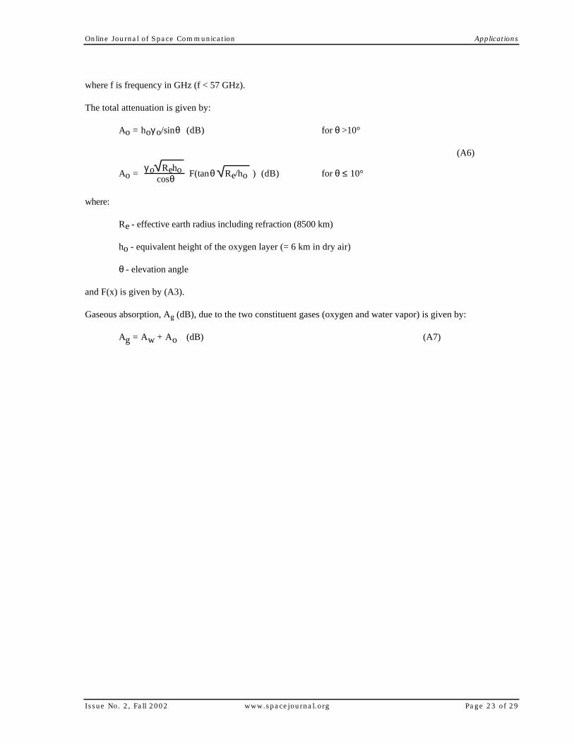
where f is frequency in GHz (f < 57 GHz).

The total attenuation is given by:

Ao = hoγ o/sinθ (dB) for θ >10°

(A6)

Ao = γ o Reho

cosθ F(tanθ Re/ho ) (dB) for θ ≤ 10°

where:

Re - effective earth radius including refraction (8500 km)

ho - equivalent height of the oxygen layer (= 6 km in dry air)


and F(x) is given by (A3).

Gaseous absorption, Ag (dB), due to the two constituent gases (oxygen and water vapor) is given by:

Ag = Aw + Ao (dB) (A7)



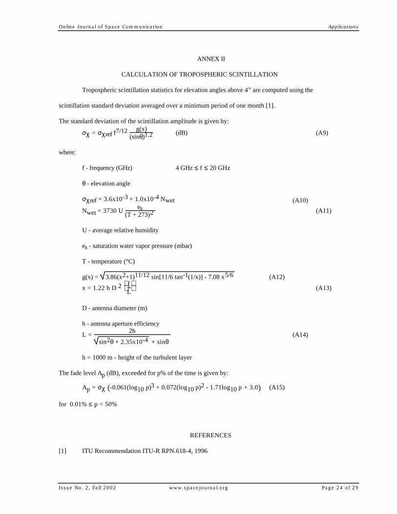
ANNEX II

CALCULATION OF TROPOSPHERIC SCINTILLATION

Tropospheric scintillation statistics for elevation angles above 4° are computed using the

scintillation standard deviation averaged over a minimum period of one month [1].

The standard deviation of the scintillation amplitude is given by:

σχ = σχref f7/12 g(x)

(sinθ)1.2 (dB) (A9)

where:

f - frequency (GHz) 4 GHz ≤ f ≤ 20 GHz


σχref = 3.6x10-3 + 1.0x10-4 Nwet (A10)

Nwet = 3730 U es

(T + 273)2 (A11)

U - average relative humidity

es - saturation water vapor pressure (mbar)

T - temperature (°C)

g(x) = 3.86(x2+1)11/12 sin[11/6 tan-1(1/x)] - 7.08 x5/6 (A12)

x = 1.22 h D 2 fL

(A13)

D - antenna diameter (m)

h - antenna aperture efficiency

L = 2h

sin2θ + 2.35x10-4 + sinθ (A14)

h = 1000 m - height of the turbulent layer

The fade level Ap (dB), exceeded for p% of the time is given by:

Ap = σχ ( )-0.061(log10 p)3 + 0.072(log10 p)2 - 1.71log10 p + 3.0 (A15)

for 0.01% ≤ p < 50%

REFERENCES

[1] ITU Recommendation ITU-R RPN.618-4, 1996



[2] R. K. Crane, "A two-component rain model for the prediction of

attenuation statistics," Radio Science, vol. 17, pp. 1371-1387, 1982

[3] M. J. Leitao and P. A. Watson, "Method for prediction of attenuation on earth-space links

based on radar measurements of the physical structure of rainfall," IEE Proc., vol. 133 Part F, pp.

429-440, 1986

[4] C. Capsoni, Fedi, F., and A. Paraboni, "A comprehensive meteorologically

oriented methodology for the prediction of wave propagation parameters

in telecommunication applications beyond 10 GHz," Radio Science, vol. 22, pp. 387-393;

1987

[5] J. E. Allnutt, "INTELSAT propagation experiments: The focus and results of recent

campaigns," IEEE Proc., vol. 81, pp. 856 - 864, 1993

[6] P. Baptista (Editor), Reference Book on Attenuation Measurement and Prediction, Second

Workshop of the Olympus Propagation Experimenters

ESA WPP-083, 1994

[7] F. Davarian (Editor), Proceedings of NAPEX XIX and APSW VII, Jet Propulsion Labs

Publication 95-15, August 1995

[8] R. K. Crane, "Estimating risk of earth-satellite attenuation prediction,"

IEEE Proc., vol. 81, pp 905 - 913, 1993

[9] J. E. Allnutt, Satellite-to-ground Radiowave Propagation, London: Peter Peregrinus Ltd.,

1989

[10] Reports of the CCIR: Report 563-4, CCIR XVllth Plenary Assembly, Dusseldorf, 1990

[11] D. S. Slobin, "Microwave noise temperature and attenuation of clouds:

Statistics of these effects at various sites in the United States, Alaska, and

Hawaii," Radio Science, vol. 17, pp. 1443-1454, 1982

[12] E. A. Altshuler and R. A. Marr, "Cloud attenuation at millimeter wavelengths," IEEE

Trans. Anten. and Prop., vol. 37, pp. 1473-1479, 1989



[13] F. Dintelmann and G. Ortgies, "A semiempirical model for cloud attenuation prediction,"

Electron. Lett., vol. 25, pp. 1487-1488, 1989

[14] E. Salonen, "Prediction models of atmospheric gases and clouds for slant path attenuation,"

Olympus Utilization Conference, Sevilla, pp. 615 - 622, 1993

[15] S. G. Warren et al., Global distribution of total cloud cover and cloud type

amounts over land, National Center for Atmospheric Research (NCAR) Technical Notes,

NCAR/TN-273, October 1986

[16] R. J. Doviak and D. S. Zrnic, Doppler Radar and Weather Observations

Orlando, Academic Press, 1984

[17] G. Ortgies, F. Rucker, and F. Dintelman, "Statistics of clear-air attenuation on satellite links

at 20 and 30 GHz," Electron. Lett., vol. 26, pp. 358 - 360,

1990

[18] L. J. Battan, Radar Observation of the Atmosphere , Chicago, University of Chicago Press,

1973

[19] W. Klassen, From snowflake to raindrop: Doppler radar observations and

simulations of precipitation, Ph.D. dissertation, University of Delft, 1989

[20] M. M. Z. Kharadly and A. S. V. Choi, "A simplified approach to the evaluation of EMW

propagation characteristics in rain and melting snow,"

IEEE Trans. Anten. and Prop., vol-36, pp. 282-296, 1988

[21] A. W. Dissanayake and N. J. McEwan, "Radar and attenuating properties of rain and bright

band," IEE Conf. Publ. 169-2, pp. 125-129, 1978

[22] A. W. Dissanayake and J. E. Allnutt, "Prediction of rain attenuation in low-latitude

regions," URSI Commission F Open Symposium: Wave propagation and remote sensing, Ravenscar,

UK, pp. 7.1.1 - 7.1.5,

June 1992,



[23] K. T. Lin, A. W. Dissanayake, and C. Cotner, "Propagation impairments on a very-low

elevation angle C-band satellite link," 15th AIAA International Communications Satellite Conf., pp.

932-936, 1994

[24] J. L. Strickland, R. L. Olsen, and H. L. Werstiuk, "Measurement of low- angle fading in

the Canadian Arctic," Ann. Telecom., vol 32, pp. 530-535, 1977

[25] ITU Radiocommunication Sector SG3 Databases, 1993

[26] Vogel, E. J., Torrence, G. W., Allnutt, J. E.; "Rain fades on low elevation

angle earth-satellite paths: Comparative assessment of the Austin, Texas,

11.2 GHz experiment," IEEE Proc., vol. 81, pp. 885 - 896, 1993

[27] Stutzman, W. L. et al.; Results from Virginia Tech Propagation

Experiment Using the Olympus Satellite 12, 20, and 30 GHz beacons

IEEE Trans. Antennas Propagat., vol. 43, pp. 54 - 62, 1995

[28] F. Davarian Editor, Presentations of the Eighth ACTS Propagation Studies

Workshop, Jet Propulsion Labs Publication D-13157, December 1995

[29] P. J. L. Maagt, et. al., "Results of 12 GHz Propagation Experiments in

Indonesia," Electron. Lett., vol. 29, pp. 1988-1990, 1993

[30] P. L. Rice and N. R. Holmberg, "Cumulative time statistics of surface

point rainfall rates," IEEE Trans. Communication, vol. 21, pp. 1131-1136, 1973

[31] ITU Recommendation ITU-R RPN.837, 1995

[32] E. J. Dutton, H. T. Dougherty, and R. F. Martin, "Prediction of European rainfall

and link performance coefficients at 8 and 30 GHz," US Dept. of Commerce

Office of Telecommunications, Tech. Report No. ACC-ACO-16-74, 1974

[33] E. J. Dutton, "Precipitation variability in the USA for microwave terrestrial

system design," US Dept. of Commerce Office of Telecommunications, OT

Report 77-134, 1977

[34] G. Feldhake, “A comparison of 11 rain attenuation models with two years of

ACTS data from seven sites,” Proceedings of 9th ACTS Propagation Studies



Workshop (APSW IX), 19-20 November, 1996

[35] A. Paraboni, “testing of rain attenuation prediction methods against the

measured data contained in the ITU-R data bank,” ITU-R Study Group 3

Document, SR2-95/6, Geneva, 1995

[36] D. L. Bryant, “Low elevation angle 11 GHz beacon measurements at Goonhilly

earth station,” BT Technology, vol. 10, No. 4, Dec 1992, pp. 68-75

[37] E. T. Salonen et. al., “Scintillation effects on total fade distribution for earth-

satellite links,” IEEE Trans. Antennas Propagat., vol. 44, pp. 23-27, 1996

[38] G. C. Gerace, E. K. Smith, “A comparison of cloud models,” IEEE Anten. and

Prop. Magazine, pp. 32-38, October 1990

[39] B. J. Mason, The Physics of Clouds, London, Oxford University Press, 1971

[40] G. L. Stephens, “Radiation profiles in extended water clouds,” Jnl. Atmospheric

Sciences, vol. 35, pp. 2111-2122, 1978



Table 3 Comparison of slant path attenuation predictions with measured data. Prediction errors shown as the mean, standard deviation, andRMS value are calculated using the plotted points on the cumulative distribution curves in Figures 3 - 15.

Site Latitude Altitude(m)

Frequency

(GHz)

ElevationAngle

Polariza-tion

Angle

M(mm)

β Measured R0.01

(mm/hr)

R-HR001

(mm/hr)

MeanError (%)

Std Error(%)

RMS Error(%)

Albertslund, DK[26,6]

55.68 30 11.19819.7729.65

4.9420.6420.64

45.070.470.4

600 0.07 25.0 23.6 2.0-2.823.6

15.415.614.2

15.515.927.6

Austin, TX[27] 30.3 100 11.198 5.75 45.0 550 0.53 75.0 76.7 10.1 12.3 15.8Blacksburg, VA

[28]37.23 646 12.5

19.7729.65

13.9313.9313.93

40.840.840.8

965 0.2 42.0 63.0 18.117.212.5

41.216.68.9

45.023.815.3

Clarksburg, MD[29]

39.2 150 20.1827.5

38.8738.87

64.6864.68

936 0.29 72.0 74.3 -13.7-8.2

9.510.9

16.613.7

Eindhoven, NL [6] 51.45 15 12.519.7729.65

26.7926.7926.79

71.7271.7271.72

770 0.1 31.0 33.3 -31.9-9.125.4

12.111.516.2

34.114.730.2

Gometz la Ville,FR [6]

48.67 10 12.519.77

30.54 72.4272.42

600 0.1 68.1 27.6 -1.1-22.4

14.114.6

14.226.7

Goonhilly, UK[26]

50.05 100 11.198 3.27 45.0 985 0.07 30.0 31.0 -16.9 15.3 22.9

Kirkkonummi, SF[6]

60.21 60 19.7729.65

12.6812.68

68.5368.53

530 0.1 44.0 25.4 -2.01.0

6.49.1

6.79.2

Lae, PNG [26] -6.45 50 12.69 72.97 26.68 3302 0.32 107.0 119.6 22.9 25.7 34.4Montreal, CA [29] 45.6 90 20.18

27.531.3931.39

66.4766.47

1020 0.11 45.0 44.9 -9.8-0.5

11.411.9

15.011.9

Oberpfaffenhofen,DE [6]

48.08 580 19.77 27.53 65.64 900 0.1 37.2 37.9 -0.2 8.8 8.8

Oklahoma, OK[29]

35.23 500 20.1827.5

48.9948.99

86.486.4

843 0.36 - 78.0 19.913.7

19.716.0

28.021.1

Reston, VA [29] 38.95 150 20.1827.5

39.139.1

64.4864.48

948 0.28 - 73.0 -5.32.3

16.716.5

17.516.6

Rome, IT [6] 41.87 32 12.519.77

32.0732.07

59.7959.79

750 0.27 70.0 64.6 -0.8-6.5

10.412.8

10.414.4

Spino d'Adda, IT[6]

45.5 84 12.519.77

30.5430.54

64.8864.88

860 0.15 45.7 49.5 -14.2-0.2

21.89.3

25.99.3

Surabaya, IND[30]

-7.3 20 11.198 20.0 45.0 2000 0.7 120.0 125.0 3.1 20.7 21.0


Issue No. 2, Fall 2002 www.spacejournal.org Page 29 of 36

0

0.5

1

1.5

2

1 10 100Percent time ordinate exceeded (P)

Clo

ud A

tten

uati

on, A

c (dB

) Predicted

Measured

Figure 1a. Comparison of measured and predicted cloud attenuation distributions in Darmstadt,Germany [17]; æ predicted, x: measured; frequency 30 GHz; elevation angle 28°; cloud

amounts use for the prediction are: total cloud cover - 63.3%, stratus - 37.3%, nimbo stratus -12%, cumulus - 4%, cumulonimbus - 2%.

0

0.5

1

1.5

2

1 10 100Percent time ordinate exceeded (P)

Clo

ud A

tten

uati

on, A

c (dB

) Predicted

Measured

Figure 1b. Cloud attenuation distribution in New York, NY [11]; æ predicted,x: measured; frequency 35 GHz; elevation angle 90°; cloud amounts use for the prediction are:

total cloud cover - 70.5%, stratus - 34.5%, nimbo stratus - 13.5%, cumulus - 3%,cumulonimbus - 2.3%.



Percent time ordinate exceeded

Signal Level (dB

)

-16

-14

-12

-10

-8

-6

-4

-2

0

0.01 0.1 1 10 100

Measured

Predicted

Figure 2a. Predicted and measured low-angle fading/tropospheric scintillationdistributions of fading on a 2° elevation angle C-band link at Clarksburg, MD [23];

frequency 3.95 GHz; measurement period: 30 days in September 1993.

Percent time ordinate exceeded

Signal Level (dB

)

-24

-20

-16

-12

-8

-4

0

0.1 1 10 100

Measured

Predicted

Figure 2b. Predicted and measured low-angle fading/tropospheric scintillationdistributions of fading on a 1° elevation angle C-band link at Eureka, Canada [24];

frequency 6 GHz.



Percent time attenuation > ordinate

Attenuation (dB

) 0

5

10

15

20

25

30

0.001 0.01 0.1 1 10

Measured 19.8 GHz

Predicted 19.8 GHz

Measured 29.7 GHz

Predicted 29.7 GHz

Number of points: 14(19.8 GHz), 12(29.7 GHz)

Figure 3. Attenuation distributions at 19.8 and 29.7 GHz at Albertslund, Denmark


Attenuation (dB

) 0

10

20

30

40

50

0.01 0.1 1 10

Measured 19.8 GHz

Predicted 19.8 GHz

Measured 29.7 GHz

Predicted 29.7 GHz


Figure 4. Attenuation distributions at 19.8 and 29.7 GHz at Blacksburg, VA, USA




Attenuation (dB

) 0

5

10

15

20

25

30

35

0.01 0.1 1 10

Measured 20.2 GHz

Predicted 20.2 GHz

Measured 27.5 GHz

Predicted 27.5 GHz


Figure 5. Attenuation distributions at 20.2 and 27.5 GHz at Clarksburg, MD, USA


Attenuation (dB

) 0

10

20

30

40

0.001 0.01 0.1 1 10

Measured 19.8 GHz

Predicted 19.8 GHz

Measured 29.7 GHz

Predicted 29.7 GHz


Figure 6. Attenuation distributions at 19.8 and 29.7 GHz at Eindhoven, Netherlands




Attenuation (dB

) 0

10

20

30

40

50

0.001 0.01 0.1 1 10

Measured 12.5 GHz

Predicted 12.5 GHz

Measured 19.8 GHz

Predicted 19.8 GHz


Figure 7. Attenuation distributions at 12.5 and 19.8 GHz at Gometz la Ville, France


Attenuation (dB

) 0

10

20

30

40

0.01 0.1 1 10

Measured 19.8 GHz

Predicted 19.8 GHz

Measured 29.7 GHz

Predicted 29.7 GHz


Figure 8. Attenuation distributions at 19.8 and 29.7 GHz at Kirkkonummi, Finland




Attenuation (dB

) 0

5

10

15

20

25

30

0.01 0.1 1 10

Measured 19.8 GHz

Predicted 20.2 GHz

Measured 27.5 GHz

Predicted 27.5 GHz


Figure 9. Attenuation distributions at 20.2 and 27.5 GHz at Montreal, Canada


Attenuation (dB

) 0

5

10

15

20

25

30

0.001 0.01 0.1 1 10

Measured 19.8 GHz

Predicted 19.8 GHz

Number of points: 15

Figure 10. Attenuation distributions at 19.8 GHz at Oberpfaffenhofen, Germany




Attenuation (dB

) 0

5

10

15

20

25

30

0.01 0.1 1 10

Measured 20.2 GHz

Predicted 20.2 GHz

Measured 27.5 GHz

Predicted 27.5 GHz


Figure 11. Attenuation distributions at 20.2 and 27.5 GHz at Oklahoma, OK, USA


Attenuation (dB

) 0

5

10

15

20

25

30

35

0.01 0.1 1 10

Measured 20.2 GHz

Predicted 20.2 GHz

Measured 27.5 GHz

Predicted 27.5 GHz


Figure 12. Attenuation distributions at 20.2 and 27.5 GHz at Reston, VA, USA




Attenuation (dB

) 0

5

10

15

20

25

30

0.01 0.1 1 10

Measured 12.5 GHz

Predicted 12.5 GHz

Measured 19.8 GHz

Predicted 19.8 GHz


Figure 13. Attenuation distributions at 12.5 and 19.8 GHz at Rome, Italy


Attenuation (dB

) 0

10

20

30

40

50

0.001 0.01 0.1 1 10

Measured 12.5 GHz

Predicted 12.5 GHz

Measured 19.8 GHz

Predicted 19.8 GHz


Figure 14. Attenuation distributions at 12.5 and 19.8 GHz at Spino 'd Adda, Italy

online journal of space communication applications -...

Documents