online inspection of 3d parts via a locally overlapping...
TRANSCRIPT

Online Inspection of 3D Parts via a Locally Overlapping Camera Network
Tolga BirdalTechnical University of Munich
Emrah Bala, Tolga ErenGravi Ltd
emrah,[email protected]
Slobodan IlicSiemens AG
Abstract
The raising standards in manufacturing demands reli-able and fast industrial quality control mechanisms. Thispaper proposes an accurate, yet easy to install multi-view,close range optical metrology system, which is suited to on-line operation. The system is composed of multiple static,locally overlapping cameras forming a network. Initially,these cameras are calibrated to obtain a global coordinateframe. During run-time, the measurements are performedvia a novel geometry extraction techniques coupled with anelegant projective registration framework, where 3D to 2Dfitting energies are minimized. Finally, a non-linear regres-sion is carried out to compensate for the uncontrollable er-rors. We apply our pipeline to inspect various geometri-cal structures found on automobile parts. While presentingthe implementation of an involved 3D metrology system, wealso demonstrate that the resulting inspection is as accurateas 0.2 mm, repeatable and much faster, compared to the ex-isting methods such as coordinate measurement machines(CMM) or ATOS.
1. IntroductionDimensional monitoring has become an important part
of manufacturing processes due to the gradually advanc-ing standards in many sectors, such as automotive (chasis),flight (wings) or energy (turbines). The welded componentsfound on the backbone of all these high-end products aresensitive and require careful manufacturing and thus, care-ful quality control. The de-facto solution to inspect thesecritical parts relies on the contact-based CMMs (coordinatemeasuring machines), which are expensive, hard to main-tain and slow to operate. These machines can neither beinstalled on the production lines nor provide 100% statis-tics on the manufactured parts. Such lack of online inspec-tion coerces many assembly lines to revert to mechanicalfixtures and apparatus to verify the quality of manufactur-ing. This has many drawbacks. First of all, notwithstand-ing the cost of assembling mechanical control fixtures, sus-taining the precision of such assembly over the long term
(a) (b)
Figure 1. Samples from the parts, our system could inspect.
requires significant amount of maintenance effort. Yet, noinformation on errors or statistics could be provided by thefixed control equipment and the inspections cannot be doc-umented. Last but not least, such inspection necessitates anoperator constantly engaging in the production process.
The bottleneck caused by the current quality control pro-cedures is addressed by Tuominen as the lack of reliable, ac-curate and generic metrology / photogrammetry techniques,which are amenable to be installed on production lines [30].Tuominen further shows that the ultimate quality controlperformance is achieved when the parts are either fully in-spected or no inspection is carried out at all. This makesCMMs an unviable option. While the industry suffers suchdrawbacks, the quality requirements imposed by the con-sumer market keep demanding more and more, stimulatingthe research on online 3D inspection [17].
This paper presents a thorough methodology on the re-search and development of an inspection unit, which ad-dresses all of the aforementioned downsides. Our system iscomposed of multiple static cameras, calibrated to a globalcoordinate frame, being able to measure arbitrary geomet-rical structures. Our algorithms are novel and carefully de-signed to fit the accuracy requirements. The resulting sys-tem is accurate within acceptable error bounds and flexible,in the sense that the design can be adopted to the inspectionof different parts with minimal modifications to the soft-ware. The entire implementation cost is lower than a CMM,while the capability of inspection is 100%, saving us from

the sampling requirement. We present quantitative compar-isons with the industry-strength commercial metrology sys-tems by evaluating our approach against an optical metrol-ogy unit (ATOS) and a standard CMM (Hexagon) both forcalibration and measurement. We also present our repeata-bility values along with the actual measurements. Finally,we demonstrate that our timings clearly outperform the stateof the art, making the system applicable to online inspec-tion. See Figure 1 for the parts we can inspect as well as theimages of the measured geometries.
The contributions of this paper are three-fold: First, wepropose an affordable and effective way to calibrate a muli-camera systetm, which is composed of local and globalcamera networks. We base our calibration on bundle ad-justment and global registration. Secondly, we develop anovel, robust, multi-view projective CAD registration pro-cedure along with a multiview edge detection scheme. Weshow that this new approach is real-time capable, while notcompromising accuracy. We review in detail the implemen-tation aspects and draw a complete picture in the design andrealization of such a multi-view metrology unit. Finally, wecarry out extensive experimental evaluation, in comparisonsto existing, state of the art metrology methodologies.
2. Prior Work
Optical metrology enjoys a history of over 30 years. Thedifferent aspects of the issue such as calibration, triangu-lation, stereo reconstruction or pose estimation have beentackled many times in computer vision literature.
Analyzing the colinearity relations, photogrammetristswere the first to use image data to conduct measurements[25, 16]. Computer vision tried to improve the lower levelsub-problems such as calibration [29, 35], pose estimation[24, 28] or SLAM [2]. In spite of the vast amount of litera-ture in computer vision, the care for accuracy and precisionis not very well established in such works.
Many commercial metrology software exist with differ-ent application areas 1,2. While being highly accurate, someof these software are not capable of measuring generic CADgeometries, but rather rely either on feature points or pre-defined markers. In contrast, the tools which could recoverarbitrary 3D geometries cannot operate on generic prior 3Dmodels. Even today, a well described, truly capable ma-chine vision technique to automate the process control re-mains to be intact [17].
Unlike the commercial arena, development of accurateand reliable close range machine vision systems is ratherunexplored in academia [17]. Jyrkinen et.al. [14] designeda system to inspect sheet metal parts, but their approach can-not be generalized to arbitrary geometries. Mostofi et. al.
1http://www.photomodeler.com/2http://www.gom.com/3d-software/atos-professional.html
[21] target a similar problem like ours. Their technique isdependent on human intervention and utilize a single mov-ing camera. Such choice is far from realtime concerns. Yet,authors report the visibility of measurement points from 6cameras, which drastically increases the number of viewsand the effort for measurement. Moreover, they report anaccuracy of 0.5mm even when the measurement points arevisible in 6 views. Such accuracy is well below what isachievable today [31]. Bergamasco et. al. [4] developeda novel method to precisely locate ellipses in images, buttheir method involves perfect overlap of views and doesn’tgeneralize to measurement of arbitrary 3D shapes. Similarto our work, Malassiotis and Strintzis developed a stereosystem to measure holes defined by CAD geometries [19].While posing the CAD fitting problem as an optimizationprocedure, just like ours, they make use of explicit primi-tive modeling, which restricts the measurement capabilities.The 3D primitives are re-generated at each step of the op-timization and this comes at the expense of computationalcomplexity, degrading the real-time (or online) capabilities.Their approach is also not applicable to triangulate arbitrary3D geometries. Moreover, all of these approaches assume aperfect calibration and lack a well established methodologyto calibrate the camera networks.
Our system is uniquely positioned in the application fieldof non-contact multi-view measurement, which was shownto be one of the most accurate metrology methods. It istuned for inspection of points of interest [18] and retrievesits power from the developments in low level and geometric3d computer vision e.g. [9, 5].
3. Proposed ApproachSystem Setup Our system consists of 48 The ImagingSource cameras providing 1280x960 pixels at 30 fps. De-pending on the installation distance, we choose either25mm, 35mm or 50mm industrial lenses. The scene is il-luminated via 10 white global LED lights, installed on theexternal skeleton. The cameras are positioned such that apoint of interest is visible to at least 3 cameras. We will re-fer to these points of interests as the measurement pointsPi ∈ R3 and to such a local camera group as the localcamera network Ci = [Ci
1,Ci2, ...,C
ik] : k < N. For the
sake of accuracy, it is highly unlikely that a single camerawould capture different measurement points and thus the lo-cal camera groups remain independent (no overlap and thusno direct calibration exists between camera groups). Theset of these K local camera groups form the global cam-era network C = C1,C2, ...,CK, in total composed of Ncameras. Eventually, our system consists of multiple lo-cal camera networks, which are calibrated to form C, theglobal camera network. In this sense, the entire network isarranged in a hierarchy, as shown in Figure 2.Target Parts For demonstration purposes, and specific to

Local Camera Groups
MeasurementPoints
Camera Network
Figure 2. System Setup. Figure depicts the locally overlappingcamera groups forming a global camera network. The shown CADmodel belongs to the actual part.
our application, we aim to inspect 15 critical points (Pi) ona 2m long and 80cm wide metal industrial automotive cha-sis. The part is shown in Figure 2. Even though our setupis capable of inspecting arbitrary CAD models from differ-ent manufacturing areas, for the purpose of clarity, we willstick to the automotive application. Typically, the geome-tries to be measured, as well as the CAD models are knownbeforehand and the accuracy is limited to 1-1.5%.Image Acquisition We control all cameras over a GigE Net-work (1000Mbit/s). The lights are strobed to be in synchwith the exposure. This prevents the multi-threaded cap-turing. We initialize each local network group per eachmeasurement, and utilize the full Gig-E bandwidth (using30fps/camera). This optimizes the speed and durability.Some images of the measured points, acquired by our sys-tem during a single runtime are shown in Figure 1(a).
3.1. Calibration
We calibrate all cameras intrinsically and extrinsically tothe same global coordinate frame. Intrinsic calibration iscarried out prior to installation using the standard methods[10, 6]. We use calibration plates made up of 3mm circularreflective dot stains. On the other hand, considering the ex-tremely non-overlapping nature of our cameras, and narrowdepth of fields, the task of extrinsic calibration is signifi-cantly difficult and crucial.
Extrinsic Calibration We use a pre-manufactured cali-bration object (reference body), The Calibrator to calibratethe absolute poses. Counter intuitively, this object is notprecisely manufactured and does not use expensive mate-rial or components, but only acts as a mounting apparatusfor circular dots, forming the relation over different cameragroups. It is produced at a CNC machine such that whenit is imaged by the multiview system, enough 3D referencepoints (calibration dots) would be visible on each camera.The shape resembles the rough approximation of the targetobject (part to be measured). We then manually attach ran-
dom circular markers so that enough overlap is created. Thecalibrator (virtually and physically) is shown in Fig. 3.
The calibration grids and random dots attached on thecalibrator are first reconstructed and bundle adjusted by tak-ing multiple overlapping shots with a high-resolution SLRcamera. We take around 128 images, and compute thepose graph (a graph, in which each edge depicts an over-lapping view) semi-automatically. The global optimizationis solved with Google Ceres [1].
After creating The Calibrator, we extrinsically calibratethe cameras by imaging the calibration plates multiple timesfor each view. During this repetitive stage, at each inspec-tion, the positions of the calibration plates are computedand subsequent measurement errors are recorded. Onceenough measurements are collected and repeatability valuesbecome acceptable, the images are gathered to be used inmultiview calibration. This way, we make sure that enoughvariance of positioning is covered. Such extrinsic calibra-tion is performed as a succeeding offline bundle adjustment(BA), where the poses and 3D structure are refined simulta-neously [11, 15].
Learning Systematic Errors Finally, the so-far ne-glected non-rigidness effects, mis-manufacturing and othersystematic errors are compensated. To achieve that, we em-ploy an error correction (bias reduction) procedure, in prin-ciple similar to [23, 22, 12]. While these methods were de-signed to perform on CMMs, we generalize the technologyto optical inspection via a learning approach. Initially, wesample a set of carefully-manufactured 3D parts. We mea-sure each of those on various CMM devices, repeatedly (5times for each) to cancel out the biases. If the desired preci-sion is verified, the median measurement per point is takenas the ground truth. We then measure the same parts withour system, repetitively, using the technique described inSec. 3.2. Based on the differences (errors) of two method-ologies (CMM and ours), we train both a Nearest Neighbourand a Support Vector Machine [7] classifier. Our featuresare the concatenated 3D point coordinates. The responses(outputs) are then the differences of these measured coor-dinates to the collected training data i.e. coordinate-wiseregressed offset from ground truth. Thanks to the accept-able mechanical precision, we could easily cover almost allthe entire space of 3D variations.
3.2. Measurement
Our measurement stage follows 4 steps: Acquisition, ex-traction of geometries of interest, fitting 3D models and tri-angulation. The part is taken with with a linear axis con-veyor belt, giving us a good initial condition. This sectionwill focus on extraction of region of interests and fittingCAD models. Note that, in our setting, we are interestedonly in measuring the 3D center coordinates, but not the
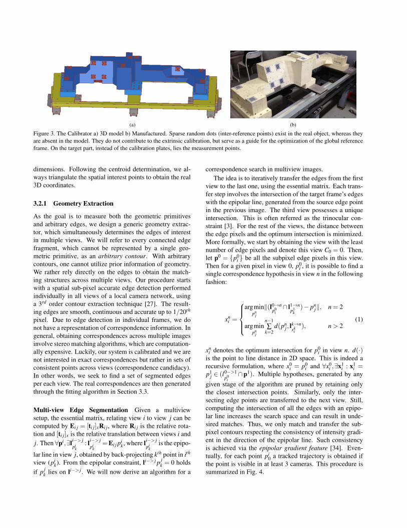
(a) (b)
Figure 3. The Calibrator a) 3D model b) Manufactured. Sparse random dots (inter-reference points) exist in the real object, whereas theyare absent in the model. They do not contribute to the extrinsic calibration, but serve as a guide for the optimization of the global referenceframe. On the target part, instead of the calibration plates, lies the measurement points.
dimensions. Following the centroid determination, we al-ways triangulate the spatial interest points to obtain the real3D coordinates.
3.2.1 Geometry Extraction
As the goal is to measure both the geometric primitivesand arbitrary edges, we design a generic geometry extrac-tor, which simultaneously determines the edges of interestin multiple views. We will refer to every connected edgefragment, which cannot be represented by a single geo-metric primitive, as an arbitrary contour. With arbitrarycontours, one cannot utilize prior information of geometry.We rather rely directly on the edges to obtain the match-ing structures across multiple views. Our procedure startswith a spatial sub-pixel accurate edge detection performedindividually in all views of a local camera network, usinga 3rd order contour extraction technique [27]. The result-ing edges are smooth, continuous and accurate up to 1/20th
pixel. Due to edge detection in individual frames, we donot have a representation of correspondence information. Ingeneral, obtaining correspondences across multiple imagesinvolve stereo matching algorithms, which are computation-ally expensive. Luckily, our system is calibrated and we arenot interested in exact correspondences but rather in sets ofconsistent points across views (correspondence candidacy).In other words, we seek to find a set of segmented edgesper each view. The real correspondences are then generatedthrough the fitting algorithm in Section 3.3.
Multi-view Edge Segmentation Given a multiviewsetup, the essential matrix, relating view i to view j can becomputed by Ei j = [ti j]xRi j, where Ri j is the relative rota-tion and [ti j]x is the relative translation between views i andj. Then ∀pi,∃li−> j
pik
: li−> jpi
k=Ei j pi
k, where li−> jpi
kis the epipo-
lar line in view j, obtained by back-projecting kth point in ith
view (pik). From the epipolar constraint, li−> j p j
k = 0 holdsif p j
k lies on li−> j. We will now derive an algorithm for a
correspondence search in multiview images.The idea is to iteratively transfer the edges from the first
view to the last one, using the essential matrix. Each trans-fer step involves the intersection of the target frame’s edgeswith the epipolar line, generated from the source edge pointin the previous image. The third view possesses a uniqueintersection. This is often referred as the trinocular con-straint [3]. For the rest of the views, the distance betweenthe edge pixels and the optimum intersection is minimized.More formally, we start by obtaining the view with the leastnumber of edge pixels and denote this view C0 = 0. Then,let p0 = p0
i be all the subpixel edge pixels in this view.Then for a given pixel in view 0, p0
i , it is possible to find asingle correspondence hypothesis in view n in the followingfashion:
xni =
argmin
pnj
‖(l0→np0
i∩ l1→n
p1k
)− pnj‖, n = 2
argminpn
j
n−1∑
k=2d(pn
j , lk→nxk
i), n > 2
(1)
xni denotes the optimum intersection for p0
i in view n. d(·)is the point to line distance in 2D space. This is indeed arecursive formulation, where x0
i = p0i and ∀x0
i ,∃x1i : x1
i =p1
j ∈ (l0−>1p0
i∩p1). Multiple hypotheses, generated by any
given stage of the algorithm are pruned by retaining onlythe closest intersection points. Similarly, only the inter-secting edge points are transferred to the next view. Still,computing the intersection of all the edges with an epipo-lar line increases the search space and can result in unde-sired matches. Thus, we only match and transfer the sub-pixel contours respecting the consistency of intensity gradi-ent in the direction of the epipolar line. Such consistencyis achieved via the epipolar gradient feature [34]. Even-tually, for each point pi
0 a tracked trajectory is obtained ifthe point is visible in at least 3 cameras. This procedure issummarized in Fig. 4.
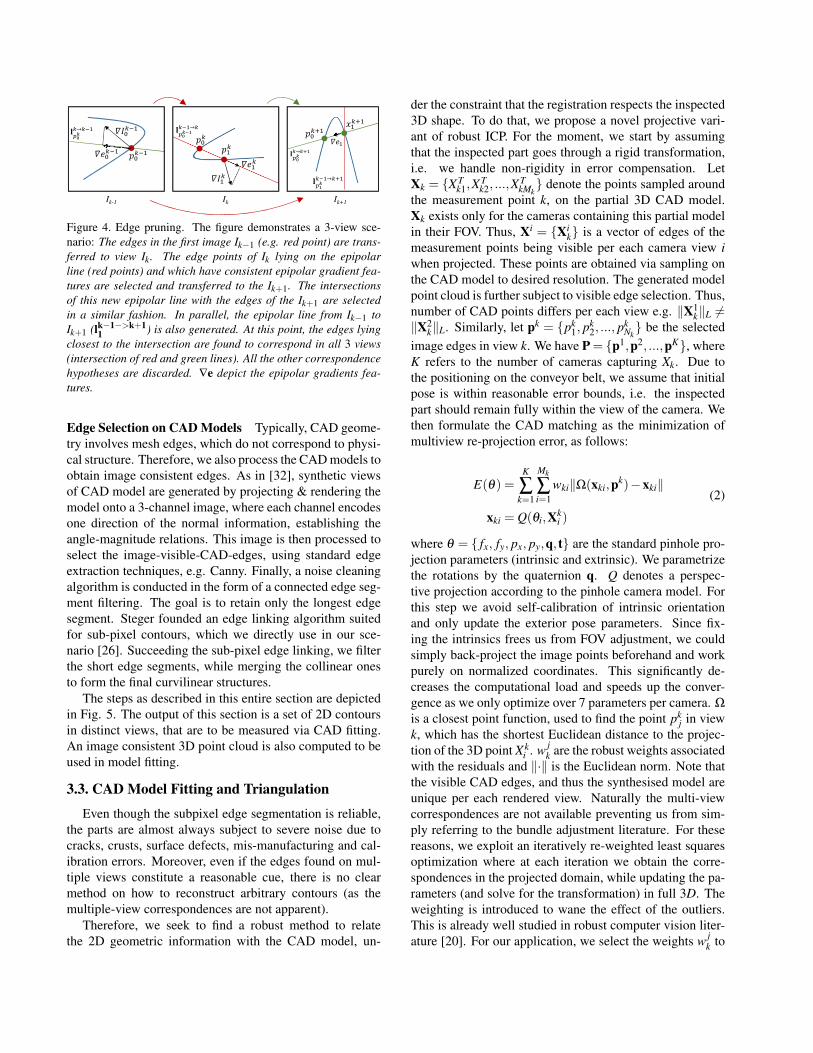
Ik-1 Ik Ik+1
→
→
→
→
Figure 4. Edge pruning. The figure demonstrates a 3-view sce-nario: The edges in the first image Ik−1 (e.g. red point) are trans-ferred to view Ik. The edge points of Ik lying on the epipolarline (red points) and which have consistent epipolar gradient fea-tures are selected and transferred to the Ik+1. The intersectionsof this new epipolar line with the edges of the Ik+1 are selectedin a similar fashion. In parallel, the epipolar line from Ik−1 toIk+1 (lk−1−>k+1
1 ) is also generated. At this point, the edges lyingclosest to the intersection are found to correspond in all 3 views(intersection of red and green lines). All the other correspondencehypotheses are discarded. ∇e depict the epipolar gradients fea-tures.
Edge Selection on CAD Models Typically, CAD geome-try involves mesh edges, which do not correspond to physi-cal structure. Therefore, we also process the CAD models toobtain image consistent edges. As in [32], synthetic viewsof CAD model are generated by projecting & rendering themodel onto a 3-channel image, where each channel encodesone direction of the normal information, establishing theangle-magnitude relations. This image is then processed toselect the image-visible-CAD-edges, using standard edgeextraction techniques, e.g. Canny. Finally, a noise cleaningalgorithm is conducted in the form of a connected edge seg-ment filtering. The goal is to retain only the longest edgesegment. Steger founded an edge linking algorithm suitedfor sub-pixel contours, which we directly use in our sce-nario [26]. Succeeding the sub-pixel edge linking, we filterthe short edge segments, while merging the collinear onesto form the final curvilinear structures.
The steps as described in this entire section are depictedin Fig. 5. The output of this section is a set of 2D contoursin distinct views, that are to be measured via CAD fitting.An image consistent 3D point cloud is also computed to beused in model fitting.
3.3. CAD Model Fitting and Triangulation
Even though the subpixel edge segmentation is reliable,the parts are almost always subject to severe noise due tocracks, crusts, surface defects, mis-manufacturing and cal-ibration errors. Moreover, even if the edges found on mul-tiple views constitute a reasonable cue, there is no clearmethod on how to reconstruct arbitrary contours (as themultiple-view correspondences are not apparent).
Therefore, we seek to find a robust method to relatethe 2D geometric information with the CAD model, un-
der the constraint that the registration respects the inspected3D shape. To do that, we propose a novel projective vari-ant of robust ICP. For the moment, we start by assumingthat the inspected part goes through a rigid transformation,i.e. we handle non-rigidity in error compensation. LetXk = XT
k1,XTk2, ...,X
TkMk denote the points sampled around
the measurement point k, on the partial 3D CAD model.Xk exists only for the cameras containing this partial modelin their FOV. Thus, Xi = Xi
k is a vector of edges of themeasurement points being visible per each camera view iwhen projected. These points are obtained via sampling onthe CAD model to desired resolution. The generated modelpoint cloud is further subject to visible edge selection. Thus,number of CAD points differs per each view e.g. ‖X1
k‖L 6=‖X2
k‖L. Similarly, let pk = pk1, pk
2, ..., pkNk be the selected
image edges in view k. We have P = p1,p2, ...,pK, whereK refers to the number of cameras capturing Xk. Due tothe positioning on the conveyor belt, we assume that initialpose is within reasonable error bounds, i.e. the inspectedpart should remain fully within the view of the camera. Wethen formulate the CAD matching as the minimization ofmultiview re-projection error, as follows:
E(θ) =K
∑k=1
Mk
∑i=1
wki‖Ω(xki,pk)−xki‖
xki = Q(θi,Xki )
(2)
where θ = fx, fy, px, py,q, t are the standard pinhole pro-jection parameters (intrinsic and extrinsic). We parametrizethe rotations by the quaternion q. Q denotes a perspec-tive projection according to the pinhole camera model. Forthis step we avoid self-calibration of intrinsic orientationand only update the exterior pose parameters. Since fix-ing the intrinsics frees us from FOV adjustment, we couldsimply back-project the image points beforehand and workpurely on normalized coordinates. This significantly de-creases the computational load and speeds up the conver-gence as we only optimize over 7 parameters per camera. Ω
is a closest point function, used to find the point pkj in view
k, which has the shortest Euclidean distance to the projec-tion of the 3D point Xk
i . w jk are the robust weights associated
with the residuals and ‖·‖ is the Euclidean norm. Note thatthe visible CAD edges, and thus the synthesised model areunique per each rendered view. Naturally the multi-viewcorrespondences are not available preventing us from sim-ply referring to the bundle adjustment literature. For thesereasons, we exploit an iteratively re-weighted least squaresoptimization where at each iteration we obtain the corre-spondences in the projected domain, while updating the pa-rameters (and solve for the transformation) in full 3D. Theweighting is introduced to wane the effect of the outliers.This is already well studied in robust computer vision liter-ature [20]. For our application, we select the weights w j
k to
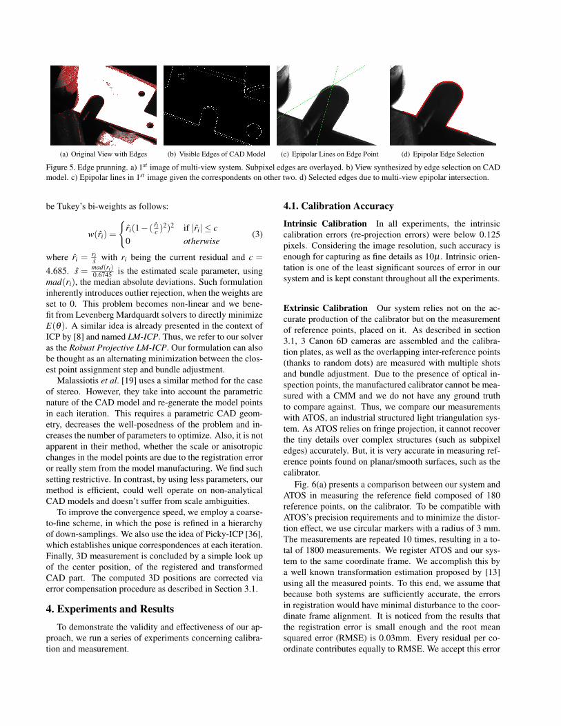
(a) Original View with Edges (b) Visible Edges of CAD Model (c) Epipolar Lines on Edge Point (d) Epipolar Edge Selection
Figure 5. Edge prunning. a) 1st image of multi-view system. Subpixel edges are overlayed. b) View synthesized by edge selection on CADmodel. c) Epipolar lines in 1st image given the correspondents on other two. d) Selected edges due to multi-view epipolar intersection.
be Tukey’s bi-weights as follows:
w(ri) =
ri(1− ( ri
c )2)2 if |ri| ≤ c
0 otherwise(3)
where ri =ris with ri being the current residual and c =
4.685. s = mad(ri)0.6745 is the estimated scale parameter, using
mad(ri), the median absolute deviations. Such formulationinherently introduces outlier rejection, when the weights areset to 0. This problem becomes non-linear and we bene-fit from Levenberg Mardquardt solvers to directly minimizeE(θ). A similar idea is already presented in the context ofICP by [8] and named LM-ICP. Thus, we refer to our solveras the Robust Projective LM-ICP. Our formulation can alsobe thought as an alternating minimization between the clos-est point assignment step and bundle adjustment.
Malassiotis et al. [19] uses a similar method for the caseof stereo. However, they take into account the parametricnature of the CAD model and re-generate the model pointsin each iteration. This requires a parametric CAD geom-etry, decreases the well-posedness of the problem and in-creases the number of parameters to optimize. Also, it is notapparent in their method, whether the scale or anisotropicchanges in the model points are due to the registration erroror really stem from the model manufacturing. We find suchsetting restrictive. In contrast, by using less parameters, ourmethod is efficient, could well operate on non-analyticalCAD models and doesn’t suffer from scale ambiguities.
To improve the convergence speed, we employ a coarse-to-fine scheme, in which the pose is refined in a hierarchyof down-samplings. We also use the idea of Picky-ICP [36],which establishes unique correspondences at each iteration.Finally, 3D measurement is concluded by a simple look upof the center position, of the registered and transformedCAD part. The computed 3D positions are corrected viaerror compensation procedure as described in Section 3.1.
4. Experiments and ResultsTo demonstrate the validity and effectiveness of our ap-
proach, we run a series of experiments concerning calibra-tion and measurement.
4.1. Calibration Accuracy
Intrinsic Calibration In all experiments, the intrinsiccalibration errors (re-projection errors) were below 0.125pixels. Considering the image resolution, such accuracy isenough for capturing as fine details as 10µ . Intrinsic orien-tation is one of the least significant sources of error in oursystem and is kept constant throughout all the experiments.
Extrinsic Calibration Our system relies not on the ac-curate production of the calibrator but on the measurementof reference points, placed on it. As described in section3.1, 3 Canon 6D cameras are assembled and the calibra-tion plates, as well as the overlapping inter-reference points(thanks to random dots) are measured with multiple shotsand bundle adjustment. Due to the presence of optical in-spection points, the manufactured calibrator cannot be mea-sured with a CMM and we do not have any ground truthto compare against. Thus, we compare our measurementswith ATOS, an industrial structured light triangulation sys-tem. As ATOS relies on fringe projection, it cannot recoverthe tiny details over complex structures (such as subpixeledges) accurately. But, it is very accurate in measuring ref-erence points found on planar/smooth surfaces, such as thecalibrator.
Fig. 6(a) presents a comparison between our system andATOS in measuring the reference field composed of 180reference points, on the calibrator. To be compatible withATOS’s precision requirements and to minimize the distor-tion effect, we use circular markers with a radius of 3 mm.The measurements are repeated 10 times, resulting in a to-tal of 1800 measurements. We register ATOS and our sys-tem to the same coordinate frame. We accomplish this bya well known transformation estimation proposed by [13]using all the measured points. To this end, we assume thatbecause both systems are sufficiently accurate, the errorsin registration would have minimal disturbance to the coor-dinate frame alignment. It is noticed from the results thatthe registration error is small enough and the root meansquared error (RMSE) is 0.03mm. Every residual per co-ordinate contributes equally to RMSE. We accept this error

0
0.01
0.02
0.03
0.04
0.05
0.06
0.07
0.08
1 2 3 4 5 6 7 8 9 10
Ave
rag
e D
evia
tio
n (
mm
)
Measurements
Min Dev Max Dev Mean Dev
(a)
-0.15 -0.1 -0.05 0 0.05 0.1 0.15
X-Errors 0 1 10 17 14 11 2
Y-Errors 2 2 10 14 9 11 7
Z-Errors 0 6 7 10 15 12 5
0
2
4
6
8
10
12
14
16
18
Fre
qu
en
cy
Error Ranges (Bins)
(b)
Figure 6. a) 180 feature points on the calibration plates are measured with ATOS and with our system, 10 times. Using all the measurements,a 3D transformation is computed between the coordinate systems and the coordinate-wise difference in the common frame is recorded. Itis shown that our system shows resemblance with ATOS system in the measurement of reference points (εmax < 0.1mm). Note that, ATOSis good at measuring such points, as the fiducials lie on planar surfaces. Yet, it will later become ineffective in measuring complicatedstructures due to fringe projection drawbacks. b) Accuracy Evaluations Histogram of registration errors to the CMM coordinate space.Bins indicate the error amount, while frequencies correspond to number of registrations. The data is taken over 55 measurements. Notethat, the errors are recorded after coordinate space registration between our system and common CMM frame. In this respect, the figureplots the accuracies relative to a CMM, which is the main measure of error in our system. Values are in milimeters.
and conclude that the calibrator is measured accurately andprecisely to achieve the desired accuracy.
4.2. Measurement Analysis
CAD Registration The iterations of refinement for a lo-cal camera group are visualized in Fig. 7. Regarding thefitting of CAD model to arbitrary subpixel contours, the fi-nal RMSE registration error is typically in the range of 0.25pixels. To quantify the numerical accuracy, we conducteda set of experiments on different types of model parts. Fig.8(a) plots the convergence of our algorithm, while Fig. 8(b)shows the inliers retained after each iteration.
Accuracy (Errors in Comparison to CMM) Error com-pensation step involves repeated measurement and registra-tion to CMM space in order to reduce the effect of sys-tematic errors. CMMs report an error of 0.01mm for thepoints of interest and stand out to be the ground truth ref-erence for our system [33]. The fact that we accept CMMresults as a baseline for our measurements, make us inter-ested in the deviations from this pseudo-ground truth. Forthis reason, we sample 55 random measurements of 5 dif-ferent parts, which are measured both with our system andwith Hexagon CMM. We then register each part from ourcoordinate space to CMM and record the errors. As this ex-periment is performed on the measured part but not on thecalibrator, we end up with an evaluation of the accuracy ofour system, with respect to the CMM. Fig. 6(b) shows ahistogram over the collected data. It is shown that the max-imum registration error is well below 0.2mm. This is bothwithin the industry standards and within the tolerances werequire.
Precision We will again refer to CMM comparisons, thistime for precision. Fig. 9 enlists a series of experi-ments conducted on 5 different measurement points. In to-tal 25 random measurements are displayed and the inter-measurement errors, which we will be referring as the re-peatability measures are tabulated. Note that the maximumerror remains significantly under 0.15mm, while appearingbelow 0.05mm most of the times.
The reported accuracy in the previous section is less thanthe precision values due to the undesired compensation er-
Figure 7. The process of CAD fitting: Red points indicate thefound edges, purple points are the model projections, while thegreen points are the extracted edge pixels. Each column is a viewand each row shows an iteration.

0
0.05
0.1
0.15
0.2
0.25
0.3
0.35
0.4
0 10 20 30 40 50
L2
Err
or
(in
pix
els
)
Iterations
Circular Oval U-shaped Rectangular
(a) Registration errors for different types of measurement points
0.7
0.75
0.8
0.85
0.9
0.95
1
0 10 20 30 40 50
% I
nli
ers
Iterations
Circular Oval U-shaped Rectangular
(b) Inliers per iteration
Figure 8. Evaluation of Registration Performance: a) Each run is started with 2.5cm translational shift and 10rotational offset. Theregistration error between the inliers is recorded at each iteration. Note that the convergence is super-linear in all types of geometricalstructures. b) Ratio of Inliers over iterations.
0
0.02
0.04
0.06
0.08
0.1
0.12
0.14
1Z 3Y 4Z 5X 5Z 5Z 5Z 7Z 8X 8Z 10X 10Y 11X 13X 13ZSta
nd
ard
De
via
tio
n (
σ)
Measurement Points
Part 1
Part 2
Part 3
Part 4
Figure 9. Repeatability results for 4 different parts, manufacturedfrom the identical CAD model. For each part, 15 out of 26 pointsare measured, 5 times each (randomly taken out of 41). The stan-dard deviation per point is plotted.
rors. In other words, the bias learned in Section 3.1 doesnot always represent the systematic components and is, toa certain extent, subject to random/unstructured noise. Forthis reason, while we are able to get measurements withmaximum 0.15mm, we introduce certain errors in the regis-tration to final coordinate space. Nevertheless, this error isnot more than 0.05mm and is tolerable in our scenario.
4.2.1 Runtime Performance
Our system aims online operations, where the complete unitis installed on an operating production line. Therefore speedplays a key role in our design. Table 1 tabulates the tim-ings for different stages of the runtime on a machine with3GhZ Intel i7 CPU and 8GB of RAM. Note that image ac-quisition (30fps) step is responsible for most of the delaysdue to synchronous capture and bandwidth. Respectively,each camera captures the individual frames with a 0.5sec ofstrobe timing (until LEDs reach the desired intensity level).No processing starts until all the cameras finish the acquisi-tion. Triangulation is only applied after every feature pointis successfully extracted.
Our system is incomparably fast w.r.t. ATOS or CMM.It is, in that sense, not a replacement for a CMM device
Table 1. Average timings in measurement stage. Timings are re-ported as an average of 10 runs. MP refers to measurement point.Even though processing of the measurement points differ, theircontribution to final runtime is averaged.
Per MP (sec) For All MPs (sec)
Image Acquisition 5,00 75,00Feature Extraction 0,30 4,50CAD Registration 0,15 2,25Bundle Adjustment 0,10 1,50
Total 83,25
but a much more effective online competitor of the existingmechanical fixtures. Inspecting a single part took 1h whenmeasured with ATOS and 45min on CMM. Both of theseresults are far from online 100% inspection.
5. Conclusions
We presented an in depth analysis of an accurate opti-cal metrology system, designed to operate on industrial set-tings, where realtime performance and durability are of con-cern. To the best of our knowledge, this was the first work toaddress jointly the calibration and measurement processes,while at the same time providing novel algorithms targetingthe fast, robust and accurate triangulation of different typesof geometries. In this regard, even though the software re-quires care in implementation, the set-up of the system isnot very complicated and can be customized without alter-ing the software. It can be configured to operate on differ-ent parts with minimal effort. It is invariant to the phys-ical system as much as possible and accounts for impre-cise manufacturing and mechanical errors at the softwarelevel. We compared our system against the industry stan-dard measurement devices, one mechanical and one optical.Our measurement results are well within the accepted toler-ances. In the future work, we will evaluate self calibrationmethods and research on the error handling mechanisms,allowing the system to recover from severe misuses.

References[1] S. Agarwal and K. Mierle. Ceres solver: Tutorial & refer-
ence. Google Inc, 2, 2012.[2] J. Aulinas, Y. Petillot, J. Salvi, and X. Llado. The slam prob-
lem: A survey. In Proceedings of the 2008 Conference on Ar-tificial Intelligence Research and Development: Proceedingsof the 11th International Conference of the Catalan Associ-ation for Artificial Intelligence, pages 363–371, Amsterdam,The Netherlands, The Netherlands, 2008. IOS Press.
[3] N. Ayache and F. Lustman. Trinocular stereo vision forrobotics. IEEE Transactions on Pattern Analysis and Ma-chine Intelligence, 13(1):73–85, 1991.
[4] F. Bergamasco, L. Cosmo, A. Albarelli, and A. Torsello. Arobust multi-camera 3d ellipse fitting for contactless mea-surements. In 3D Imaging, Modeling, Processing, Visual-ization and Transmission (3DIMPVT), 2012 Second Interna-tional Conference on, pages 168–175. IEEE, 2012.
[5] P. J. Besl and N. D. McKay. Method for registration of 3-dshapes. In Robotics-DL tentative, pages 586–606. Interna-tional Society for Optics and Photonics, 1992.
[6] J.-Y. Bouguet. Camera calibration toolbox for m atlab. 2004.[7] C. Cortes and V. Vapnik. Support-vector networks. Machine
learning, 20(3):273–297, 1995.[8] A. W. Fitzgibbon. Robust registration of 2d and 3d point sets.
Image and Vision Computing, 21(13):1145–1153, 2003.[9] R. I. Hartley and A. Zisserman. Multiple View Geometry
in Computer Vision. Cambridge University Press, ISBN:0521540518, second edition, 2004.
[10] J. Heikkila. Geometric camera calibration using circular con-trol points. Pattern Analysis and Machine Intelligence, IEEETransactions on, 22(10):1066–1077, 2000.
[11] L. Heng, B. Li, and M. Pollefeys. Camodocal: Automatic in-trinsic and extrinsic calibration of a rig with multiple genericcameras and odometry. In Intelligent Robots and Systems(IROS), 2013 IEEE/RSJ International Conference on, pages1793–1800. IEEE, 2013.
[12] G. Hermann. Geometric error correction in coordinate mea-surement. In Acta Polytechnica Hungarica, volume 4, pages47–62, 2007.
[13] B. K. Horn. Closed-form solution of absolute orientationusing unit quaternions. JOSA A, 4(4):629–642, 1987.
[14] K. Jyrkinen, M. Ollikainen, V. Kyrki, J. P. Varis, andH. Kalviainen. Optical 3d measurement in the quality as-surance of formed sheet metal parts. In Proceedings of In-ternational Conference on Pattern Recognition, volume 120,page 12, 2003.
[15] F. Kahlesz, C. Lilge, and R. Klein. Easy-to-use calibrationof multiple-camera setups. In Workshop on Camera Calibra-tion Methods for Computer Vision Systems (CCMVS2007),Mar. 2007.
[16] R. Loser, T. Luhmann, and L. H. PMU. The programmableoptical 3d measuring system pom-applications and perfor-mance. International Archives of Photogrammetry and Re-mote Sensing, 29:533–533, 1993.
[17] T. Luhmann. Close range photogrammetry for industrial ap-plications. ISPRS Journal of Photogrammetry and RemoteSensing, 65(6):558–569, 2010.
[18] T. Luhmann, F. Bethmann, B. Herd, and J. Ohm. Com-parison and verification of optical 3-d surface measurementsystems. The international archives of the photogrammetry,remote sensing and spatial information sciences, 37:51–56,2008.
[19] S. Malassiotis and M. Strintzis. Stereo vision system for pre-cision dimensional inspection of 3d holes. Machine Visionand Applications, 15(2):101–113, 2003.
[20] P. Meer. Robust techniques for computer vision. In Emergingtopics in computer vision, pages 107–190, 2004.
[21] N. Mostofi, F. Samadzadegan, S. Roohy, and M. Nozari. Us-ing vision metrology system for quality control in automo-tive industries. ISPRS-International Archives of the Pho-togrammetry, Remote Sensing and Spatial Information Sci-ences, 1:33–37, 2012.
[22] S. Phillips, B. Borchardt, A. Abackerli, C. Shakarji,D. Sawyer, P. Murray, B. Rasnick, K. Summerhays, J. Bald-win, R. Henke, et al. The validation of cmm task specificmeasurement uncertainty software. In Proc. of the ASPE2003 summer topical meeting Coordinate Measuring Ma-chines, 2003.
[23] S. Sartori and G. Zhang”. ”geometric error measurementand compensation of machines”. volume ”44”, pages ”599 –609”, ”1995”.
[24] S. Savarese and L. Fei-Fei. Multi-view object categorizationand pose estimation. In Computer Vision, pages 205–231.Springer, 2010.
[25] C.-T. Schneider and K. Sinnreich. Optical 3-d measure-ment systems for quality control in industry. InternationalArchives of Photogrammetry and Remote Sensing, 29:56–56,1993.
[26] C. Steger. An unbiased detector of curvilinear structures.IEEE Trans. Pattern Anal. Mach. Intell., 20(2):113–125, Feb.1998.
[27] A. Tamrakar and B. Kimia. No grouping left behind: Fromedges to curve fragments. In Computer Vision, 2007. ICCV2007. IEEE 11th International Conference on, pages 1–8,Oct 2007.
[28] A. Tejani, D. Tang, R. Kouskouridas, and T.-K. Kim. Latent-class hough forests for 3d object detection and pose estima-tion. In Computer Vision ECCV 2014, volume 8694 of Lec-ture Notes in Computer Science, pages 462–477. SpringerInternational Publishing, 2014.
[29] R. Y. Tsai. A versatile camera calibration technique for high-accuracy 3d machine vision metrology using off-the-shelf tvcameras and lenses. Robotics and Automation, IEEE Journalof, 3(4):323–344, 1987.
[30] V. Tuominen. Cost modeling of inspection strategies in auto-motive quality control. Engineering Management Research,1(2):p33, 2012.
[31] V. Uffenkamp. State of the art of high precision industrialphotogrammetry. In Third international workshop on accel-erator alignment., 1993.
[32] M. Ulrich, C. Wiedemann, and C. Steger. Combining scale-space and similarity-based aspect graphs for fast 3d objectrecognition. Pattern Analysis and Machine Intelligence,IEEE Transactions on, 34(10):1902–1914, Oct 2012.
[33] N. Van Gestel. Determining Measurement Uncertainties ofFeature Measurements on CMMs (Bepalen van meetonzeker-heden bij het meten van vormelementen met CMMs). 2011.
[34] E. Vincent and R. Laganiere. Matching with epipolar gradi-ent features and edge transfer. In Image Processing, 2003.ICIP 2003. Proceedings. 2003 International Conference on,volume 1, pages I–277. IEEE, 2003.
[35] Z. Zhang. A flexible new technique for camera calibration.Pattern Analysis and Machine Intelligence, IEEE Transac-tions on, 22(11):1330–1334, 2000.
[36] T. Zinßer, J. Schmidt, and H. Niemann. A refined icp algo-rithm for robust 3-d correspondence estimation. In ImageProcessing, 2003. ICIP 2003. Proceedings. 2003 Interna-tional Conference on, volume 2, pages II–695. IEEE, 2003.