online auction markets
TRANSCRIPT

Online Auction Markets
by
Song Yao
Department of Business AdministrationDuke University
Date:
Approved:
Carl Mela, Chair
Han Hong
Wagner Kamakura
Andres Musalem
Dissertation submitted in partial fulfillment of the requirements for the degree ofDoctor of Philosophy in the Department of Business Administration
in the Graduate School of Duke University2009
Abstract(Business Administration)
Online Auction Markets
by
Song Yao
Department of Business AdministrationDuke University
Date:
Approved:
Carl Mela, Chair
Han Hong
Wagner Kamakura
Andres Musalem
An abstract of a dissertation submitted in partial fulfillment of the requirements forthe degree of Doctor of Philosophy in the Department of Business Administration
in the Graduate School of Duke University2009

Copyright c© 2009 by Song YaoAll rights reserved except the rights granted by the
Creative Commons Attribution-Noncommercial Licence
Abstract
Central to the explosive growth of the Internet has been the desire of dispersed buy-
ers and sellers to interact readily and in a manner hitherto impossible. Underpinning
these interactions, auction pricing mechanisms have enabled Internet transactions in
novel ways. Despite this massive growth and new medium, empirical work in mar-
keting and economics on auction use in Internet contexts remains relatively nascent.
Accordingly, this dissertation investigates the role of online auctions; it is composed
of three essays.
The first essay, “Online Auction Demand,” investigates seller and buyer interac-
tions via online auction websites, such as eBay. Such auction sites are among the
earliest prominent transaction sites on the Internet (eBay started in 1995, the same
year Internet Explorer was released) and helped pave the way for e-commerce. Hence,
online auction demand is the first topic considered in my dissertation. The second
essay, “A Dynamic Model of Sponsored Search Advertising,” investigates sponsored
search advertising auctions, a novel approach that allocates premium advertising
space to advertisers at popular websites, such as search engines. Because sponsored
search advertising targets buyers in active purchase states, such advertising venues
have grown very rapidly in recent years and have become a highly topical research
domain. These two essays form the foundation of the empirical research in this dis-
sertation. The third essay, “Sponsored Search Auctions: Research Opportunities in
Marketing,” outlines areas of future inquiry that I intend to pursue in my research.
iv

Of note, the problems underpinning the two empirical essays exhibits a common
form, that of a two-sided network wherein two parties interact on a common plat-
form (Rochet and Tirole, 2006). Although theoretical research on two-sided markets
is abundant, this dissertation focuses on their use in e-commerce and adopts an em-
pirical orientation. I assume an empirical orientation because I seek to guide firm
behavior with concrete policy recommendations and offer new insights into the actual
behavior of the agents who interact in these contexts. Although the two empirical
essays share this common feature, they also exhibit notable differences, including the
nature of the auction mechanism itself, the interactions between the agents, and the
dynamic frame of the problem, thus making the problems distinct. The following
abstracts for these two essays as well as the chapter that describes my future research
serve to summarize these contributions, commonalities and differences.
Online Auction Demand
With $40B in annual gross merchandise volume, electronic auctions comprise a sub-
stantial and growing sector of the retail economy. For example, eBay alone generated
a gross merchandise volume of $14.4B during the fourth quarter of 2006. Concurrent
with this growth has been an attendant increase in empirical research on Internet
auctions. However, this literature focuses primarily on the bidder; I extend this re-
search to consider both seller and bidder behavior in an integrated system within a
two-sided network of the two parties. This extension of the existing literature enables
an exploration of the implications of the auction house’s marketing on its revenues as
well as the nature of bidder and seller interactions on this platform. In the first essay,
I use a unique data set of Celtic coins online auctions. These data were obtained
from an anonymous firm and include complete bidding and listing histories. In con-
trast, most existing research relies only on the observed website bids. The complete
bidding and listing histories provided by the data afford additional information that
v

illuminates the insights into bidder and seller behavior such as bidder valuations and
seller costs.
Using these data from the ancient coins category, I estimate a structural model
that integrates both bidder and seller behavior. Bidders choose coins and sellers list
them to maximize their respective profits. I then develop a Markov Chain Monte
Carlo (MCMC) estimation approach that enables me, via data augmentation, to infer
unobserved bidder and seller characteristics and to account for heterogeneity in these
characteristics. My findings indicate that: i) bidder valuations are affected by item
characteristics (e.g., the attributes of the coin), seller (e.g. reputation), and auction
characteristics (e.g., the characteristics of the listing); ii) bidder costs are affected
by bidding behavior, such as the recency of the last purchase and the number of
concurrent auctions; and iii) seller costs are affected by item characteristics and
the number of concurrent listings from the seller (because acquisition costs evidence
increasing marginal values).
Of special interest, the model enables me to compute fee elasticities, even though
no variation in historical fees exists in these data. I compute fee elasticities by
inferring the role of seller costs in their historical listing decision and then imputing
how an increase in these costs (which arises from more fees) would affect the seller’s
subsequent listing behavior. I find that these implied commission elasticities exceed
per-item fee elasticities because commissions target high value sellers, and hence,
commission reductions enhance their listing likelihood. By targeting commission
reductions to high value sellers, auction house revenues can be increased by 3.9%.
Computing customer value, I find that attrition of the largest seller would decrease
fees paid to the auction house by $97. Given that the seller paid $127 in fees,
competition offsets only 24% of the fees paid by the seller. In contrast, competition
largely in the form of other bidders offsets 81% of the $26 loss from buyer attrition.
In both events, the auction house would overvalue its customers by neglecting the
vi
effects of competition.
A Dynamic Model of Sponsored Search Advertising
Sponsored search advertising is ascendant. Jupiter Research reports that expen-
ditures rose 28% in 2007 to $8.9B and will continue to rise at a 26% Compound
Annual Growth Rate (CAGR), approaching half the level of television advertising
and making sponsored search advertising one of the major advertising trends af-
fecting the marketing landscape. Although empirical studies of sponsored search
advertising are ascending, little research exists that explores how the interactions of
various agents (searchers, advertisers, and the search engine) in keyword markets
affect searcher and advertiser behavior, welfare and search engine profits. As in the
first essay, sponsored search constitutes a two-sided network. In this case, bidders
(advertisers) and searchers interact on a common platform, the search engine. The
bidder seeks to maximize profits, and the searcher seeks to maximize utility.
The structural model I propose serves as a foundation to explore these outcomes
and, to my knowledge, is the first structural model for keyword search. Not only
does the model integrate the behavior of advertisers and searchers, it also accounts
for advertisers competition in a dynamic setting. Prior theoretical research has as-
sumed a static orientation to the problem whereas prior empirical research, although
dynamic, has focused solely on estimating the dynamic sales response to a single
firm’s keyword advertising expenditures.
To estimate the proposed model, I have developed a two-step Bayesian estimator
for dynamic games. This approach does not rely on asymptotics and also facilitates
a more flexible model specification.
I fit this model to a proprietary data set provided by an anonymous search engine.
These data include a complete history of consumer search behavior from the site’s web
log files and a complete history of advertiser bidding behavior across all advertisers.
vii

In addition, the data include search engine information, such as keyword pricing and
website design.
With respect to advertisers, I find evidence of dynamic bidding behavior. Ad-
vertiser valuation for clicks on their sponsored links averages about $0.27. Given
the typical $22 retail price of the software products advertised on the considered
search engine, this figure implies a conversion rate (sales per click) of about 1.2%,
well within common estimates of 1-2% (gamedaily.com). With respect to consumers,
I find that frequent clickers place a greater emphasis on the position of the sponsored
advertising link. I further find that 10% of consumers perform 90% of the clicks.
I then conduct several policy simulations to illustrate the effects of change in
search engine policy. First, I find that the search engine obtains revenue gains
of nearly 1.4% by sharing individual level information with advertisers and enabling
them to vary their bids by consumer segment. This strategy also improves advertiser
profits by 11% and consumer welfare by 2.9%. Second, I find that a switch from a
first to second price auction results in truth telling (advertiser bids rise to advertiser
valuations), which is consistent with economic theory. However, the second price
auction has little impact on search engine profits. Third, consumer search tools lead
to a platform revenue increase of 3.7% and an increase of consumer welfare of 5.6%.
However, these tools, by reducing advertising exposure, lower advertiser profits by
4.1%.
Sponsored Search Auctions: Research Opportunities in Marketing
In the final chapter, I systematically review the literature on keyword search and
propose several promising research directions. The chapter is organized according to
each agent in the search process, i.e., searchers, advertisers and the search engine, and
reviews the key research issues for each. For each group, I outline the decision process
involved in keyword search. For searchers, this process involves what to search, where
viii

to search, which results to click, and when to exit the search. For advertisers, this
process involves where to bid, which word or words to bid on, how much to bid, and
how searchers and auction mechanisms moderate these behaviors. The search engine
faces choices on mechanism design, website design, and how much information to
share with its advertisers and searchers. These choices have implications for customer
lifetime value and the nature of competition among advertisers. Overall, I provide
a number of potential areas of future research that arise from the decision processes
of these various agents.
Foremost among these potential areas of future research are i) the role of alter-
native consumer search strategies for information acquisition and clicking behavior,
ii) the effect of advertiser placement alternatives on long-term profits, and iii) the
measure of customer lifetime value for search engines. Regarding the first area, a
consumer’s search strategy (i.e., sequential search and non-sequential search) affects
which sponsored links are more likely to be clicked. The search pattern of a con-
sumer is likely to be affected by the nature of the product (experience product vs.
search product), the design of the website, the dynamic orientation of the consumer
(e.g., myopic or forward-looking), and so on. This search pattern will, in turn, af-
fect advertisers payments, online traffic, sales, as well as the search engine’s revenue.
With respect to the second area, advertisers must ascertain the economic value of
advertising, conditioned on the slot in which it appears, before making decisions such
as which keywords to bid on and how much to bid. This area of possible research
suggests opportunities to examine how advertising click-through and the number of
impressions differentially affect the value of appearing in a particular sponsored slot
on a webpage, and how this value is moderated by an appearance in a non-sponsored
slot (i.e., a slot in the organic search results section). With respect to the third area
of future research, customer value is central to the profitability and long-term growth
of a search engine and affects how the firm should allocate resources for customer
ix

acquisition and retention.
Organization
This dissertation is organized as follows. After this brief introduction, the essay, “On-
line Auction Demand,” serves as a basis that introduces some concepts of auctions as
two-sided markets. Next, the second essay, “A Dynamic Model of Sponsored Search
Advertising,” extends the first essay by considering a richer context of bidder compe-
tition and consumer choice behavior. Finally, the concluding chapter, which outlines
my future research interests, considers potential extensions that pertain especially
to sponsored search advertising.
x

Contents
Abstract iv
List of Tables xv
List of Figures xvii
Acknowledgements xviii
1 Online Auction Demand 1
1.1 Introduction . . . . . . . . . . . . . . . . . . . . . . . . . . . . . . . . 1
1.2 The E-auction Context and Data . . . . . . . . . . . . . . . . . . . . 7
1.2.1 Rules of the Auction House and Participants’ Decision Processes 7
1.2.2 Data . . . . . . . . . . . . . . . . . . . . . . . . . . . . . . . . 11
1.3 An Integrated Model of Bidders and Sellers . . . . . . . . . . . . . . . 14
1.3.1 Key Assumptions and Nomenclature . . . . . . . . . . . . . . 14
1.3.2 Model Overview . . . . . . . . . . . . . . . . . . . . . . . . . . 19
1.3.3 The Second Stage – Bidder’s Model . . . . . . . . . . . . . . . 20
1.3.4 The First Stage – Seller’s Model . . . . . . . . . . . . . . . . . 25
1.4 Estimation . . . . . . . . . . . . . . . . . . . . . . . . . . . . . . . . . 31
1.4.1 The Conditional Likelihood of Bidder Model . . . . . . . . . . 31
1.4.2 The Conditional Likelihood of Seller Model . . . . . . . . . . . 32
1.4.3 Augmented Full Posterior Distribution . . . . . . . . . . . . . 33
1.5 Results . . . . . . . . . . . . . . . . . . . . . . . . . . . . . . . . . . . 34
xi

1.6 Managerial Implications . . . . . . . . . . . . . . . . . . . . . . . . . 37
1.6.1 Auction House Pricing . . . . . . . . . . . . . . . . . . . . . . 38
1.6.2 Customer Value in a Two-sided Market . . . . . . . . . . . . . 43
1.6.3 Elasticities of Seller Feedback Scores . . . . . . . . . . . . . . 46
1.7 Conclusion . . . . . . . . . . . . . . . . . . . . . . . . . . . . . . . . . 47
2 A Dynamic Model of Sponsored Search Advertising 52
2.1 Introduction . . . . . . . . . . . . . . . . . . . . . . . . . . . . . . . . 52
2.2 Recent Literature . . . . . . . . . . . . . . . . . . . . . . . . . . . . . 58
2.3 Empirical Context . . . . . . . . . . . . . . . . . . . . . . . . . . . . 62
2.3.1 Data Description . . . . . . . . . . . . . . . . . . . . . . . . . 63
2.4 Model . . . . . . . . . . . . . . . . . . . . . . . . . . . . . . . . . . . 69
2.4.1 Consumer Model . . . . . . . . . . . . . . . . . . . . . . . . . 69
2.4.2 Advertiser Model . . . . . . . . . . . . . . . . . . . . . . . . . 78
2.5 Estimation . . . . . . . . . . . . . . . . . . . . . . . . . . . . . . . . . 84
2.5.1 An Overview . . . . . . . . . . . . . . . . . . . . . . . . . . . 84
2.5.2 First Step Estimation . . . . . . . . . . . . . . . . . . . . . . . 85
2.5.3 Second Step Estimation . . . . . . . . . . . . . . . . . . . . . 87
2.5.4 Sampling Chain . . . . . . . . . . . . . . . . . . . . . . . . . . 87
2.6 Results . . . . . . . . . . . . . . . . . . . . . . . . . . . . . . . . . . . 88
2.6.1 First Step Estimation Results . . . . . . . . . . . . . . . . . . 88
2.6.2 Second Step Estimation Results . . . . . . . . . . . . . . . . . 95
2.7 Policy Simulations . . . . . . . . . . . . . . . . . . . . . . . . . . . . 98
2.7.1 Policy Simulation I: Alternative Webpage Design . . . . . . . 100
2.7.2 Policy Simulation II: Segmentation and Targeting . . . . . . . 101
2.7.3 Policy Simulation III: Incorporating Disaggregate Level Data 102
xii

2.7.4 Policy Simulation IV: Alternative Auction Mechanisms . . . . 103
2.8 Conclusion . . . . . . . . . . . . . . . . . . . . . . . . . . . . . . . . . 104
3 Sponsored Search Auctions: Research Opportunities in Marketing109
3.1 Introduction . . . . . . . . . . . . . . . . . . . . . . . . . . . . . . . . 109
3.2 An Introduction of Sponsored Search Auctions . . . . . . . . . . . . . 111
3.3 Internet Users . . . . . . . . . . . . . . . . . . . . . . . . . . . . . . . 114
3.3.1 Choosing Engines and Keywords . . . . . . . . . . . . . . . . 114
3.3.2 Choosing Search Websites to Investigate . . . . . . . . . . . . 115
3.3.3 Choosing Links to Click . . . . . . . . . . . . . . . . . . . . . 122
3.4 Advertisers . . . . . . . . . . . . . . . . . . . . . . . . . . . . . . . . 125
3.4.1 Which Search Engines and Which Words to Bid . . . . . . . . 125
3.4.2 How to Measure the Value of an Advertising Spot . . . . . . . 127
3.4.3 How Much to Bid . . . . . . . . . . . . . . . . . . . . . . . . . 130
3.5 Search Engines . . . . . . . . . . . . . . . . . . . . . . . . . . . . . . 138
3.5.1 Optimal Auction Design . . . . . . . . . . . . . . . . . . . . . 139
3.5.2 Search Query Results . . . . . . . . . . . . . . . . . . . . . . . 142
3.5.3 Targeted Marketing–Product Differentiation Across Users . . . 144
3.5.4 Customer Value in a Two-sided Market . . . . . . . . . . . . . 146
3.5.5 Price Dispersion Among Advertisers’ Goods . . . . . . . . . . 147
3.5.6 Click Fraud . . . . . . . . . . . . . . . . . . . . . . . . . . . . 149
3.6 Conclusion . . . . . . . . . . . . . . . . . . . . . . . . . . . . . . . . . 150
4 Appendices 152
4.1 Appendices for “Online Auction Demand” . . . . . . . . . . . . . . . 152
4.1.1 Proof of Theorem 1.1 . . . . . . . . . . . . . . . . . . . . . . . 152
4.1.2 Proof of Theorem 1.2 . . . . . . . . . . . . . . . . . . . . . . . 155
xiii

4.1.3 MCMC Sampling Chain . . . . . . . . . . . . . . . . . . . . . 156
4.1.4 Monte Carlo Simulation . . . . . . . . . . . . . . . . . . . . . 167
4.2 Appendices for “A Dynamic Model of Sponsored Search Advertising” 169
4.2.1 Two Step Estimator . . . . . . . . . . . . . . . . . . . . . . . 169
4.2.2 MCMC Sampling Chain . . . . . . . . . . . . . . . . . . . . . 181
4.2.3 Policy Simulations . . . . . . . . . . . . . . . . . . . . . . . . 189
Bibliography 193
Biography 204
xiv

List of Tables
1.1 Listing Features Summary Statistics . . . . . . . . . . . . . . . . . . 12
1.2 Auctions Summary Statistics . . . . . . . . . . . . . . . . . . . . . . . 12
1.3 Bidders Summary Statistics . . . . . . . . . . . . . . . . . . . . . . . 13
1.4 Feedback Summary Statistics . . . . . . . . . . . . . . . . . . . . . . 14
1.5 Private Value vs. Common Value – Regression of Bids on the Numberof Bidders . . . . . . . . . . . . . . . . . . . . . . . . . . . . . . . . . 15
1.6 Posterior Means and Standard Deviations of Model Parameters . . . 35
1.7 Fee and Commission Price Elasticities . . . . . . . . . . . . . . . . . . 39
1.8 Revenue Percentage Changes with Alternative Pricing Schedules . . . 40
1.9 Revenue Effects with Targeting of Commissions and Fees . . . . . . . 42
1.10 The Value of the Largest Customer . . . . . . . . . . . . . . . . . . . 44
1.11 Indirect Value Due to Listings and Prices . . . . . . . . . . . . . . . . 46
1.12 Seller Feedback Score Elasticity . . . . . . . . . . . . . . . . . . . . . 47
2.1 Bids Summary Statistics . . . . . . . . . . . . . . . . . . . . . . . . . 66
2.2 Product Compatibility . . . . . . . . . . . . . . . . . . . . . . . . . . 67
2.3 Product Attributes and Downloads . . . . . . . . . . . . . . . . . . . 68
2.4 Bidding Function Estimates . . . . . . . . . . . . . . . . . . . . . . . 90
2.5 Alternative Numbers of Latent Segments . . . . . . . . . . . . . . . . 92
2.6 Consumer Model Estimates . . . . . . . . . . . . . . . . . . . . . . . 93
2.7 Searching Behavior of Consumers . . . . . . . . . . . . . . . . . . . . 94
xv

2.8 Alternative Models . . . . . . . . . . . . . . . . . . . . . . . . . . . . 96
2.9 Value per Click Parameter Estimates . . . . . . . . . . . . . . . . . . 96
3.1 Research Opportunities of Sponsored Search Auctions . . . . . . . . . 151
4.1 The Specification of the Priors . . . . . . . . . . . . . . . . . . . . . . 157
4.2 Monte Carlo Simulation Results . . . . . . . . . . . . . . . . . . . . . 168
4.3 The Specification of the Priors for Advertiser Bidding Model . . . . . 182
4.4 The Specification of the Priors for Consumer Model . . . . . . . . . . 184
4.5 The Specification of the Priors for Second Step Estimation . . . . . . 188
xvi
List of Figures
1.1a Payment Flows in a Two-sided Market . . . . . . . . . . . . . . . . . 4
1.1b Pricing Decision of the Auction House in a Two-sided Market . . . . 4
1.1c The Value of a Customer in a Two-Sided Market . . . . . . . . . . . 5
1.2 The Seller Decision . . . . . . . . . . . . . . . . . . . . . . . . . . . . 8
1.3 The Bidder Decision . . . . . . . . . . . . . . . . . . . . . . . . . . . 10
1.4 Observed Bids Vs. Simulated Bids . . . . . . . . . . . . . . . . . . . 36
2.1 Searching “chocolate phone” Using A Specialized Search Engine . . . 65
2.2 Consumer Decisions . . . . . . . . . . . . . . . . . . . . . . . . . . . . 70
2.3 Advertiser Decisions . . . . . . . . . . . . . . . . . . . . . . . . . . . 79
2.4 Distribution of Values per Download . . . . . . . . . . . . . . . . . . 97
3.1 Sponsored Search Advertising Example . . . . . . . . . . . . . . . . . 112
3.2 The Relationship among Customers, Advertisers and Search Engines 113
3.3 A Search Engine with the Easy Comparison Tool . . . . . . . . . . . 117
xvii

Acknowledgements
I would like to dedicate this work to my family. My parents and my sister taught
me the value of education and always encouraged me to pursue my dreams. More
importantly, I would like to dedicate this dissertation to my wife, Hong Ke, and my
son, Nathan, for their support, kindness, and patience during this splendid journey
of personal growth. Without my family’s unconditional love, I could not have done
it.
I would like to thank my dissertation committee members for making this experi-
ence of Ph.D. education enjoyable and fulfilling. They helped me to transition from
a student to a researcher.
I am especially grateful to my dissertation Chair, Carl Mela. Carl has been a
marvelous advisor. He has always been able to guide me in the right direction at
different stages of this dissertation process. His support helped me to overcome
various obstacles during my Ph.D. study. Carl’s insights and advice enabled me
to gain a much better appreciation of the issues addressed in this work, and more
crucially, to shape my future research interests.
I would also thank my committee members Han Hong, Wagner Kamakura, Andres
Musalem, and my ad hoc committee member, Rick Staelin. Their mentorship and
support not only enhanced my insights and creativity throughout the production of
this work, but also have strengthened the foundation for my future research.
Likewise, I am appreciative of Debu Purohit. Together with Carl and Rick, Debu
xviii

served as one of my academic advisors during my first year at Duke. The discussions
with my first year advisors helped me to achieve a clearer understanding of the field
of Business Administration.
My thanks also go to the faculty at the Fuqua School of Business for always
being supportive, kind and, more significantly, treating students as colleagues. I have
become more confident due to such a nurturing and friendly environment. Also, the
industrious work of the faculty assistants at the Fuqua School of Business, especially
Kathy Joiner and Bobbie Clinkscales, made my life much easier.
Lastly, I thank my fellow students for drinking beers together, sharing joys and
frustrations, and in particular, listening to my “tedious” research for hours and
providing helpful feedback. Our friendships will continue.
xix

1
Online Auction Demand
1.1 Introduction
Commensurate with the ascendancy of the Internet, e-commerce has witnessed ex-
plosive growth. According to a US Census Bureau report in Q1-2006, US e-commerce
retail sales increased by 25.4% while retail sales across all channels grew at a more
restrained 8.1%.1 Much of this growth is due to online auctions. For example, eBay
alone had 222 million confirmed registered users by the end of Q4-2006. These users
generated a gross merchandise volume of $14.4 billion across 610 million auctions, a
growth rate of 23%.2 This compares to quarterly sales of roughly $100 billion in the
US Grocery industry.3
Concurrent with this growth, empirical/econometric research pertaining to the
design and conduct of auctions has seen increased attention in marketing of late
(Chakravarti et al., 2002). For example, Park and Bradlow (2005) analyze “whether,
1 Resource: US Census Bureau(2006, Q1), Quarterly Retail E-Commerce Sales. (http://www.census.gov/mrts/www/ecomm.html)
2 Resource: eBay Inc. 4qtr-2006 Financial Releases.3 Resource: “Grocery Stores and Supermarkets Industry Profile Excerpt”, First Research, 2005.
(http://www.firstresearch.com/Industry-Research/Grocery-Stores-and-Supermarkets.html)
1

who, when and how much” to bid under an online auction context; Chan et al.
(2007) consider bidders’ willingness to pay for an auction; and Bradlow and Park
(2007) investigate how bidders’ behaviors evolve over the course of an auction. This
research has led to some important insights regarding the nature of bidder behavior
in auctions. We extend this empirical literature by considering the behavior of sellers
at the auction site. An integrated analysis of bidder and seller behavior has pivotal
implications for the marketing policies of the auction house, such as the fees the
auction house sets, the rules used to conduct the auction, or an assessment of the
value of its customers (Greenleaf and Sinha, 1996).
Given our interest in seller behavior and its attendant policy implications, we
focus on structural models of auction behavior. Such models enable one to ascertain
unobserved characteristics of bidders and sellers, such as their latent costs of bidding
and listing and their ramifications for auction fees, mechanism design and/or cus-
tomer value.4 Like the marketing literature to which we alluded above, structural
model research in the context of auctions has largely focused on bidder behavior
(Reiss and Wolak, 2005). For example, Bajari and Hortacsu (2003) propose a struc-
tural model to explore the determinants of bidders bidding behaviors. The paper
assesses the effects of endogenous bidder entry into an auction and is among the
first to model structural bidding behavior in the context of electronic auctions. As
such, it forms a cornerstone of the bidder model in our research. Jofre-Bonet and
Pesendorfer (2003) consider dynamic bidding behavior arising from capacity con-
straints in a repeated procurement auction game. They find these constraints lead
to higher bids because a winning bid increases capacity constraints in the subsequent
period; this reduced incentive to win is commensurate with higher bids. Campo et al.
(2002) investigate an auction model with possible risk averse bidders and propose a
4 As discussed in Laffont and Vuong (1996), auction data are well-suited for structural models asauctions are asymmetric information games and the data generating process is strategy-driven. Fora more complete summary of structural models of auctions, see Reiss and Wolak (2005).
2
semiparametric estimation procedure to test the risk neutrality of bidders. There is
also a rich literature focusing on the question of identification of empirical auction
models, e.g., Paarsch (1992), Guerre et al. (2000), Athey and Haile (2002), Hong and
Shum (2002) and Haile et al. (2003). In sum, this literature has further enriched our
insights regarding strategic buying behavior in the context of auctions.
Our model supplements the structural auctions literature in a number of regards:
First, we integrate both bidder and seller behavior; that is, we do not presume
seller behavior regarding the number of items to list to be exogenous. In practice,
both bidders and sellers are strategically interactive, and it is reasonable to suspect
that the market equilibrium is determined by their interactions. The integration of
bidder and seller behavior in auctions is an example of a two-sided market, wherein
multiple parties interact on a platform (Rochet and Tirole, 2006; Tucker, 2005).
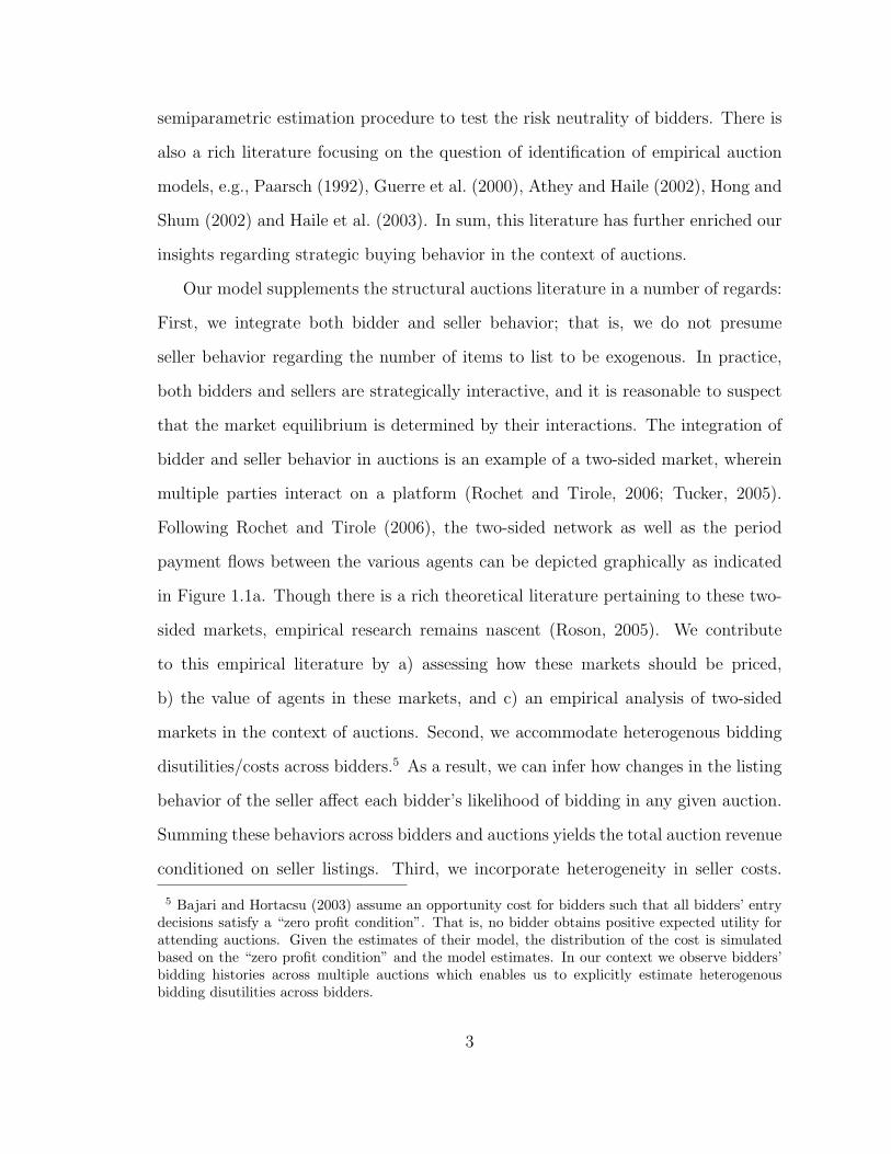
Following Rochet and Tirole (2006), the two-sided network as well as the period
payment flows between the various agents can be depicted graphically as indicated
in Figure 1.1a. Though there is a rich theoretical literature pertaining to these two-
sided markets, empirical research remains nascent (Roson, 2005). We contribute
to this empirical literature by a) assessing how these markets should be priced,
b) the value of agents in these markets, and c) an empirical analysis of two-sided
markets in the context of auctions. Second, we accommodate heterogenous bidding
disutilities/costs across bidders.5 As a result, we can infer how changes in the listing
behavior of the seller affect each bidder’s likelihood of bidding in any given auction.
Summing these behaviors across bidders and auctions yields the total auction revenue
conditioned on seller listings. Third, we incorporate heterogeneity in seller costs.
5 Bajari and Hortacsu (2003) assume an opportunity cost for bidders such that all bidders’ entrydecisions satisfy a “zero profit condition”. That is, no bidder obtains positive expected utility forattending auctions. Given the estimates of their model, the distribution of the cost is simulatedbased on the “zero profit condition” and the model estimates. In our context we observe bidders’bidding histories across multiple auctions which enables us to explicitly estimate heterogenousbidding disutilities across bidders.
3

Figure 1.1a: Payment Flows in a Two-sided Market
Figure 1.1b: Pricing Decision of the Auction House in a Two-sided Market
Heterogeneity in costs implies that the number of auctions listed can change in
response to bidders’ valuations or auction house fees. Fourth, we integrate Bayesian
statistics and structural models in the context of auctions, which is relatively novel
in marketing and economics.6 The Bayesian approach enables considerable flexibility
in model specification (Rossi et al., 1996).
Together, these innovations enable us to assess how changes in auction house
strategies (such as fee schedules or auction design) affect the number of auctions and
the corresponding bidding behaviors even in the absence of any observed variation
6 Bajari and Hortacsu (2003) is a notable exception.
4

Figure 1.1c: The Value of a Customer in a Two-Sided Market
in these strategies. This in turn affects the number of items upon which bidders
bid. As a result, the auction house can forecast the effect of fee changes on the
equilibrium number of items listed by sellers and the prices that buyers pay for these
items. Closing prices and the number of items listed factor into the auction house
revenue. In this manner it is possible to compute price elasticities for the auction
house fees in order to evaluate its pricing strategy. In contrast, it is difficult to
assess these elasticities by regressing seller listings and closing prices on fees, because
there is often little variation in fees from which to infer changes in auction demand
and prices. eBay, for example, changes its fees about once per year, leaving few
observations from which to infer price response. Moreover, to infer price response,
one would need to use observations regarding fee changes that are many years old
and it is unclear whether data from the distant past remain valid given the changing
sample composition of customers over time.
Using the imputed price-demand system, we conclude (via a pricing policy exper-
iment wherein we manipulate auction house prices) that changing fees can increase
auction house revenue by 3.9% with a targeted pricing strategy and 2.9% with a
uniform pricing strategy. Much of this gain arises from emphasizing per item fees
over commissions. Lower commissions disproportionately attract higher valuation
5

items by increasing per item profits. This further suggests that categories with a
greater prevalence of high value items such as art should emphasize per item fees
over commissions. Figure 1.1b depicts the pricing policy experiment graphically in
the context of the two-sided market.
A corollary benefit of the foregoing innovations is that they enable one to assess
the short-term value of a customer in a two-sided market.7 Information regarding
customer value is useful for assessing how much to invest in retaining a customer
(exemplified via a targeted coupon or rebate from the auction house). A common
approach toward assessing customer value is to simply tally the total commissions
and fees the seller pays to the auction house. However, were that seller to depart the
system, some bidders would switch to other sellers. Moreover, with less competition,
the remaining sellers are inclined to list more items. Both behaviors affect equilibrium
prices. A proper accounting of these competitive effects offsets about 24% of the
fees paid by a departing seller. An analogous argument can be constructed for
valuing buyers. The lost revenue resulting from the attrition of a buyer is offset
by the remaining bidders who bid on the items that the attriting buyer would have
purchased. In addition, the departure of a buyer can incent a seller to reduce listings
in response to a decrease in the expected price they will receive. We find other bidders
bidding on the items of the attrited buyer offset about 81% of the lost revenue from
the attrited buyer. Stated differently, valuing agents without regard to competitive
interactions overstates the value of the seller by 1/3 and the value of a buyer in
excess of 400%. These conclusions arise from a policy experiment wherein we assess
the impact of an attrited customer on equilibrium revenue. This policy experiment
is reflected graphically in Figure 1.1c. It is worth noting that Figures 1.1a–1.1c
suggest that our model could also be useful in addressing further policy experiments
7 By short-term, we refer to the value of the customer over the duration of our data. Long-term,or life-time value would consider the infinite horizon value of a customer.
6
such as assessing the profitability of auction fees to the buyer.
In sum, explicitly considering seller and bidder behavior in a joint system or two-
sided market enables one to a) attain a better understanding of how sellers make
listing decisions and b) engage policy simulations to help the auction house implement
its marketing strategies. With these goals in mind, the paper is organized as follows.
Section 1.2 describes the bidding mechanism used by many online auction houses.
This characterization motivates the structure of the game. Next, we present our
data and some exploratory analyses to develop insights regarding auction behavior,
especially with respect to the interaction between bidders and sellers. We then detail
the model and corresponding estimation approach in Section 1.3 and 1.4. Results of
this model are detailed in Section 1.5. Using the results, Section 1.6 overviews the
managerial implications, including the impact of fee changes, valuing customers and
gauging the effect of seller’s reputation in auctions. This discussion is followed by
Section 3.6, which concludes the paper with a summary of findings, limitations and
future research directions.
1.2 The E-auction Context and Data
A necessary precursor to modeling auction behavior is a complete characterization
of the process of listing and bidding an item. Hence, in this section, we preface our
model discussion with a characterization of the data and auction mechanism. As
the firm supplying the data wishes to remain anonymous, we describe the process in
somewhat general terms, beginning with the decisions of the seller.
1.2.1 Rules of the Auction House and Participants’ Decision Processes
Listing
A seller commences an auction by listing an item online. To list an item, the seller
must be registered with the auction firm and pay a small listing fee. For an additional
7
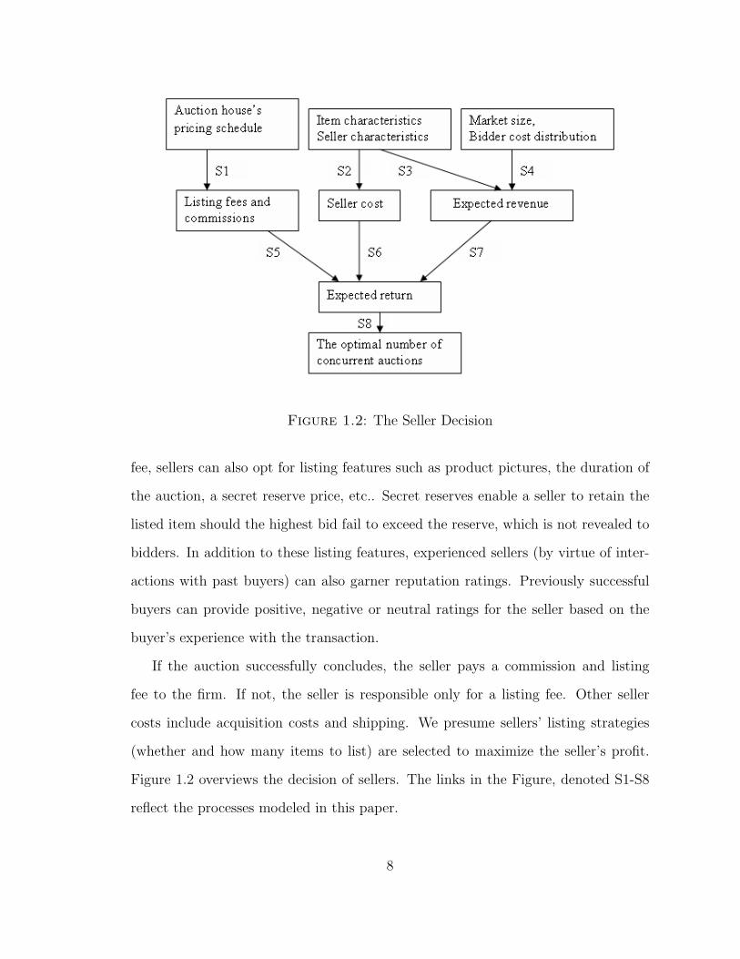
Figure 1.2: The Seller Decision
fee, sellers can also opt for listing features such as product pictures, the duration of
the auction, a secret reserve price, etc.. Secret reserves enable a seller to retain the
listed item should the highest bid fail to exceed the reserve, which is not revealed to
bidders. In addition to these listing features, experienced sellers (by virtue of inter-
actions with past buyers) can also garner reputation ratings. Previously successful
buyers can provide positive, negative or neutral ratings for the seller based on the
buyer’s experience with the transaction.
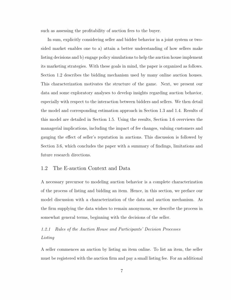
If the auction successfully concludes, the seller pays a commission and listing
fee to the firm. If not, the seller is responsible only for a listing fee. Other seller
costs include acquisition costs and shipping. We presume sellers’ listing strategies
(whether and how many items to list) are selected to maximize the seller’s profit.
Figure 1.2 overviews the decision of sellers. The links in the Figure, denoted S1-S8
reflect the processes modeled in this paper.
8

Bidding
Bidders typically initiate the bidding process via a key-word search to locate relevant
sellers, categories and items of interest. The results of this search list pertinent items
open to bidding, sorted by price and time left until the auction concludes. Upon
finding an item of interest, a bidder can bid immediately (if registered) or place the
item onto a “watch list” for subsequent monitoring and potential bidding.
The bidding mechanism used by the auction house is called “proxy bidding”.
With proxy bidding, a bidder enters an auction prior to its conclusion and submits
their bid. The website will then act as a “proxy” to bid for the bidder by entering
a bid on behalf of the user whenever the user is outbid (to some pre-determined
maximum level). For example, assume a bidder intends to bid no more than $10.00
for a given item. Suppose further that the item’s current price is $1.00 with a bid
increment of $0.50. By submitting a $10.00 proxy bid to the website, the auction
site enters a bid of $1.50 on behalf of the bidder. If another bidder enters and bids
$5.00, the proxy bid automatically becomes $5.50. If a subsequent bid of $15.00
materializes, the high bid changes to $10.50 and the first bidder receives an E-mail
notification that they were outbid. The bidder can then choose whether to increase
their bid or quit the auction altogether.
Upon placing the highest bid, the bidder wins the auction and makes a payment
to the seller that equals to the second highest bid. It is the responsibility of the seller
and the winning bidder to settle payment and delivery issues. We presume that a
bidder’s bidding strategy (whether and how much to bid) is selected to maximize
their expected profits. More specifically, we assume the bidder will bid if the expected
return from doing so exceeds the cost. Figure 1.3 overviews bidding decision process.
The links in the Figure, denoted B1-B10 reflect the bidder behaviors we model.
9
Figure 1.3: The Bidder Decision
Seller-Bidder Interactions
The foregoing discussion suggests why it is desirable to model bidder and seller
behaviors jointly. First, the bidder’s costs and returns affect the optimal bidding
levels and decisions to bid. Strategic sellers form expectations regarding bidding
levels and bidder costs. Predicated upon these expectations, sellers make listing
decisions. Bidders, who are also strategic, in turn make bidding decisions conditional
on the seller’s listing behavior. Hence, seller and bidder decisions are interdependent.
Accordingly, the auction house directly affects the seller’s profits and the number of
items sellers list by varying auction fees. The effects of a fee change propagate to
bidders by altering the decisions of sellers. To exemplify this point, we next describe
our data and present some descriptive statistics regarding bidder-seller interactions.
10

1.2.2 Data
We use a unique data set generously presented by an international auction house
that prefers to remain anonymous. The focal category is collectible Celtic coins. We
selected this category because it is fairly isolated, inasmuch as bidders in this category
tend not to buy other types of coins. This mitigates considerations regarding seller
and bidder behavior in other categories. The data were collected from November,
2004 to April, 2005 and encompass 816 auctions8 listed by 57 sellers over 189 days.
Of these listings, 72.2% were finally sold. The number of bidders is 925. The auctions
data comprise several files, including a listing file, a bidding file, and a demographics
file for the bidders and sellers. We describe each in turn.
Listing File
The listing data include, for each item listed, the unique seller ID, a text descrip-
tion of the item, and the item’s listing characteristics. These characteristics include
“picture”, whether the seller includes at least one picture of the item in their listing;
“subtitle”, a paid feature which present detailed descriptions under the listing title;
“gallery picture”, an icon-size picture of the item beside the title when the auction
is presented by the search engine; “store”, which enables a seller to group items on a
single web page; “bold”, in which the auction title is shown as bold characters; and
“featured listing”, wherein the item listing is displayed near the top of the searching
results. For each listing, we also observe the exact value of the secret reserve price,
if chosen by the seller. We include the percentage statistics of the listing features in
Table 1.1. This Table shows “Bold”, “Featured Listing” and “Secret Reserve” are
seldom used by sellers.
8 This number reflects the exclusion of 36 largely inactive sellers who only listed one auction inthe 6-month period. The sparse observation per seller make it difficult to make inferences regardingtheir behavior and identify seller-specific effects (that said, our key results are robust to theirinclusion). By omitting these 36 sellers/auctions, we also lose 10 bidders (out of a pool of 935
11

Table 1.1: Listing Features Summary Statistics
Listing Features PercentagePicture 90.21Subtitle 4.57Gallery Picture 30.90Bold 1.85Featured Listing 0.54Online Store 28.00Secrete Reserve 2.33Number of Auctions 816
Table 1.2: Auctions Summary Statistics
Mean Std. Dev. Median Min. Max.Book Value $ 93.39 96.87 55 3 675Final Price/Book Value 0.86 1.31 0.48 0 4.25Secret Reserve Price/Book Value (Obs.=19) 1.33 2.23 0.54 0.13 9.06Minimum Bid/Book Value 0.15 0.46 0.1 4.00E-05 11.65Average Listing Fees per Auction $ 0.74 1.59 0.35 0.25 21.40Average Commissions per Auctions $ 1.00 1.99 0.39 0 22.62Duration (Days) 7.01 1.14 7 1 10Lapse Since Last Listing (Days) 53.23 42.22 42 1 180Number of Concurrent Listings By the Same Seller 1.65 1.3 1 1 12Number of Sellers per Week 14.96 3.84 15 9 23
To obtain the prevailing market prices of listed items, we collect the data from
two sources. The first one is an online coins catalog (www.vcoins.com), which is
widely recognized among the coin collectors community. A second source is from
the book Coins of England and the United Kingdom, Standard Catalogue of British
Coins, 41st Edition. We report the price information together with some other listing
information in Table 1.2.
The final price is close to book value. While auction durations vary from 1 day
to 10 days, most auctions last 7 days. Hence, we define the interval of analysis (e.g.,
whether to list) to be weekly. All auctions employ an open reserve price, denoted
minimum bid, that is observed by all buyers. A handful of sellers (2.3%) also employ
a secret reserve. Though its level is not known to the bidders, the presence of a secret
bidders) who bid only in those auctions.
12

Table 1.3: Bidders Summary Statistics
Mean Std. Dev. Median Min. Max.Number of Bidders per Auction 2.58 2.94 1.50 0 18Number of Bids per Auction 4.17 5.44 2 0 31Lapse Since Last Winning (Days) 61.37 41.73 56 7 189Number of Concurrent Auctions Attended per Week 1.02 0.24 1 1 15Number of Bidders per Week 64.46 29.82 58.50 18 160
reserve is common knowledge and can therefore enter the bidder utility function.
Bidding File
The bidding data include a detailed bidding history of each unique bidder ID through
the 6 months. Thus we observe every bid a bidder submits and the time the bid
was made. This includes the highest bid that occurred in each auction, which is
not normally observed for most sealed second-price online auction data. Table 1.3
presents some summary statistics of the data.
The majority of bidders only attend one auction per week, suggesting that pur-
chases are not concentrated in the hands of a few buyers. We also observe little evi-
dence of buyer reselling as none are cross listed as sellers and they tend to purchase
only one coin at a time. In addition, the total number of items listed is dominated
by a few large sellers.9 Together, these observations reflect a market comprised of
many collectors buying from a set of dealers and that it is therefore appropriate to
model the bidders and sellers as different agents. The lapse since last winning varies
dramatically across bidders and suggests the importance of capturing heterogeneity
across bidders.
Demographic File: Seller and Buyer Feedback
The demographic file includes demographic information for sellers and bidders. With
the exception of participants’ feedback scores, these demographics are incomplete, so
9 The seller market is moderately concentrated with a Herfindahl Index of 0.12. The top 15 sellersaccount for 80% of all listings.
13

Table 1.4: Feedback Summary Statistics
Mean Std. Dev. Median Min. Max.Seller Feedback Rating 1886.25 2554.18 821.5 1 13600
Bidder Feedback Rating 186.55 273.55 89 -1 2167
we focus only on feedback scores. We report the feedback scores in Table 1.4. Among
the participants population, 5.5% are females, 53.6% are males, and the balance did
not report their gender.
While feedback scores for both sellers and bidders evidence considerable variation,
the scores for sellers are more diverse. Also, as a group, sellers have a higher mean
and median feedback score than bidders, which suggests that sellers are more active
and experienced than bidders.
1.3 An Integrated Model of Bidders and Sellers
1.3.1 Key Assumptions and Nomenclature
We detail a number of assumptions used to make our modeling approach more effi-
cient. Most are standard assumptions in the literature. These are as follows:
• First, we assume a private value (PV) auction. The assumptions of a private
value (PV) auction and a common value (CV) auction lead to different inter-
pretations of the data and methods of inference (Milgrom and Weber, 1982).10
To justify the PV assumption, we use the empirical test first proposed by
Milgrom and Weber (1982). The method is also discussed and implemented in
other literature (Athey and Haile, 2002; Bajari and Hortacsu, 2003; Haile et al.,
10 There are two types auctions based on the degree of independence across bidders’ valuation foran auctioned item: private value and common value. In a private value model, bidders evaluate theitem independently from others and such valuations are private information. Knowledge of others’valuations does not affect one’s own valuation. In contrast, the common value model assumes allbidders’ valuations are identical ex post (even though each bidder may have an idiosyncratic exante valuation).
14

Table 1.5: Private Value vs. Common Value – Regression of Bids on the Number ofBidders
All Bids Last BidsIntercept -0.05 (0.16) 0.34 (0.21)Log(Number of Bidders) 0.48* (0.03) 0.41* (0.04)Log(Book Value) 0.65* (0.03) 0.57* (0.04)Log(Seller Feedback) -0.06* (0.01) -0.05* (0.02)Secret Reserve Price 0.49* (0.10) 0.56* (0.15)Gallery Picture 0.03 (0.04) 0.10* (0.05)Log(Bidder Feedback) 0.01 (0.01) 0.01 (0.02)Number of Obs. Used 3344 2117Adjusted R2 0.29 0.25
2003; Paarsch, 1992). The idea of the test is to exploit the relationship between
the number of bidders and bids. With the existence of the “winner’s curse”
in common value auctions, the average bids in an N–bidder auction should
be lower than a (N − 1)–bidder auction.11 In comparison, such a relationship
does not hold under a private value assumption. In Table 1.5, we present
the results from two IV regressions of (log) bids on (log) number of bidders.
The first regression uses all bids while the second only uses the last bids of
each bidder. Using (log) minimum bid, “Bold” and “Featured Listing” as
instruments for the number of bidders, the regression coefficients for the number
of bidders on prices are positive and significant. Thus we proceed with the
Private Value assumption in our structural empirical model. Under the PV
assumption auctions reduce to a second price, sealed bid auction (Vickrey,
1961; Milgrom and Weber, 1982).
• Second, we assume bidders’ private valuation signals for a given item are drawn
independently from the value distribution, another common assumption in the
11 In common value settings, winning bidders are those most likely to have over-estimated anitem’s value (which is the reason for their highest bids). Note that all bidders have the same expost valuation. Thus, winning bidders typically over-pay, hence the “winner’s curse”. The bidderwill lower their bid to offset this potential over-estimation.
15

literature, denoted independent value (IV). Given the context of bidders bid-
ding modestly priced items over the Internet (with dispersed bidders and lim-
ited interpersonal contact), we also believe this to be a reasonable assump-
tion. Note that this assumption does not imply valuations are independent as
changes in the mean of the distribution affect all bidders. For example, the
seller use of a gallery can affect all buyers’ valuations. As noted by Reiss and
Wolak (2005), the alternative assumption of Affiliated Values (AV) has seen
scant attention because it is difficult to characterize the equilibria of these auc-
tions (requiring additional strict assumptions). Thus, like most research that
precedes ours, we model an Independent Private Value (IPV) auction on the
bidder side.
• Third, we consider a static game with bidders and sellers. This assumption is
not as restrictive as it initially appears, as we can control for dynamics such
as an inter-temporal budget constraint via a reduced-form approximation. We
leave more formal resolution of the dynamic problem for future research; this
would entail solving a dynamic program, ensuring the equilibrium is unique,
and identifying this solution from the data, all of which may be a contribution
in its own right, if feasible. As noted in our literature review, this is a prevalent
assumption.
• Fourth, we model cross-auction interdependence by specifying a diminishing
marginal value for each additional auction attended. In contexts wherein bid-
ders routinely bid on multiple concurrent auctions, there exist the potential for
other interdependencies in strategic bidding behavior (Brusco and Lopomo,
2009). However, Table 1.3 indicates there exists little multiple auction bidding
suggesting that this is an appropriate approximation. Accommodating strate-
gic cross-item bidding adds considerable complexity to the model with little
16

attendant benefit given the limited occurrence of these events in our data.
• Fifth, we assume the sellers’ choices of listing features (e.g., reservation prices,
gallery, etc.) are exogenously given. Endogenizing this decision admits a multi-
plicity of listing feature equilibria, rendering such a specification of little value
for assessing how the pricing of features affects demand for these features.
Moreover, endogenizing feature choices implies the need to compute an equi-
librium for every set of features, which leads to the curse of dimensionality and
quickly becomes infeasible (or requiring an approximate as opposed to an exact
solution). Thus, we leave it to future research in combinatorial optimization
to assess whether this problem is resolvable and restrict our analysis to the
effect of listing fees and commissions.12 We note prior research considers seller
behavior to be altogether exogenous.
• Sixth, our model estimation assumes bidders and sellers are fully informed
about the number of bidders in the market and the bidder valuation and bidder
cost distributions. The assumption that bidders and sellers are aware of the
value distribution may be a reasonable approximation in light of the ability
of bidders and sellers to monitor auction outcomes over time by observing
historical bids on the web site. Most preceding research makes this assumption
on the bidder side and we extend this precedent to the seller side. The number
of sellers and bidders can also be observed from the web site. We explore
12 It is possible to endogenize the reservation price decision. A benefit of this approach is that sucha model formalizes the decision making process on the part of the seller. The cost is that endoge-nous reservation prices make the model more complex (i.e., introduces additional noise along withexplanation). Given the trade-off, we test such a model and find that endogenizing reservation pricehas only a negligible effect on parameter estimates (the correlation between the median parameterestimates in this model and our base formulation is 0.985). Further, the endogenous reservationprice model evidences lower fit (by decreasing the log marginal likelihood for listings and bids from-21278.41 to -22150.82). Therefore we do not pursue this development further in this paper. Asan aside, endogenizing reservation prices leads to reservation pricing equilibria that may not beunique; as such the model has more limited applicability in the context of policy simulations.
17

the assumption that sellers and bidders are fully informed about the buyer
cost distribution by estimating a model wherein we assume their knowledge is
limited only to the mean of this distribution. We find this model leads to a
0.9% decrease in the log marginal likelihood.13 For our policy simulations we
invoke the additional assumption sellers form expectations about the number
of sellers in the market and the distribution of seller costs.
• Seventh, we assume risk neutral and symmetric bidders, consistent with previ-
ous literature (e.g. Bajari and Hortacsu, 2003). Symmetry implies that bidders
draw private valuations from the same distribution, ex ante. However, upon
receiving their signals, they differ in their individual valuations. Moreover,
heterogeneity in bidder costs implies bidders are asymmetric in their bidding
utilities even when they ex ante have the same expected valuation for an item
(as utility is value less costs). Accordingly, the symmetry assumption is not as
restrictive as it may appear. Nonetheless, we explore this assumption following
the approach of Athey et al. (2004) and Flambard and Perrigne (2004), who
posit asymmetry in valuations arises from bidders’ idiosyncratic characteristics.
Following this approach, we regress final bids on observed bidder characteris-
tics including bidder feedback, time lapse since last bid, and time lapse since
last win. We find none of these effects to be statistically significant, consistent
with the assumption of symmetric bidders.
• Eighth, we assume that the focal auction house is operating as a monopoly.
We believe it is a reasonable approximation due to the dominant market share
of the auction house in the category and market we consider. Its scale leads
13 The assumption that bidders and sellers know the full bidder cost distribution results in a logmarginal likelihood of -21278.4. Restricting this knowledge to only the mean of this distributionyields a log marginal likelihood of -21469.9. Hence the data support the assumption that biddersand sellers are aware of the bidder cost distribution.
18

to strong network effects (for example, a seller can reach a large number of
bidders) making it difficult for bidders and sellers to successfully buy and list
items with competing houses and reducing the likelihood they will defect over a
small change in fees. Evidence for this assumption is afforded by a small share
competitor who lowered their fees with no effect on the share of the considered
firm.
• Ninth, we focus on behaviors within one category and abstract any cross cat-
egory bidding, listing implications (e.g., Haile et al., 2003, and others). We
select our category of analysis to comport with this assumption.
1.3.2 Model Overview
We assume the bidder-seller game in any given period (e.g. weekly in our data) as
follows:
• In Stage 0, each seller is endowed with some types of coins associated with a
seller-item specific opportunity cost for acquiring the coin(s). For each type of
these coins, an optimal listing feature combination is exogenously determined
by the item’s and seller’s characteristics. This combination of listing features,
in conjunction with seller and item characteristics, determines the distribution
of valuations of bidders regarding the item. Each bidder will then draw a
valuation for the item from this distribution.
• In Stage 1, conditioned upon house fees, the acquisition costs and the expected
revenue, the seller assesses the expected return. The seller then decides whether
to list and, if so, how many items to list for each type conditional on the
expected returns. More specifically, we presume the seller lists the precise
number of items that leads to the highest profit over all alternative numbers
of items listed.
19
• In Stage 2, for each auction, each bidder decides whether to participate in the
auction and, if so, submits the optimal bid. As noted by Bajari and Hortacsu
(2003), sniping (last-minute bidding) is the unique Bayesian Nash equilibrium
for on-line auctions and, as a result, these auctions are equivalent to sealed-
bid second price auctions. Even in the absence of sniping, when the IPV
assumption sustains, auctions are equivalent to sealed-bid second price auctions
(Vickrey, 1961; Milgrom and Weber, 1982), i.e., the timing of bid submission
does not affect the optimal bidding strategy. As such, we abstract away from
within-auction bidding dynamics.
Given we assume that the listing feature choice and cost function are exogenously
determined in Stage 0, we only detail the game for Stage 1 (how many items to list)
and Stage 2 (conditioned on listings, how much to bid). We solve this problem using
backward induction, beginning with the bidder model first. As a further prelude
to our model, some clarifications of the indices we use are necessary. We define
i = 1, 2, ..., I to indicate sellers and j = 1, 2, ..., J to denote the bidders in the
market. Different types t = 1, 2, ..., T of items are available for auction (e.g., Celtic
silver drachm of Alexander III vs. Celtic silver tetradrachm of Philip II). The same
seller can initiate multiple auctions for the same type of coin. We use n = 1, 2, ..., N
to index auctions.
1.3.3 The Second Stage – Bidder’s Model
The Valuation of A Bidder
For the n-th auction with item t listed by seller i, each potential bidder draws a
valuation from the distribution with p.d.f. g(vijtn|µit, σ), where vijtn stands for bidder
j’s valuation for the item (for example, a specific coin). We presume the bidder’s
valuation for a given type of item auctioned by a given seller remains the same
across auctions, i.e., vijtn = vijtn′ . This ensures that the primary source of variation
20

in unobserved valuations occurs across bidders as opposed to within bidder volatility
in valuations, as the within person variation is likely to be relatively constant over
a short span of time (recall, we can allow longitudinal variation in bidder valuations
via observed changes in item and seller characteristics in conjunction with listing
features). We define µit and σ to be the value distribution mean and standard
deviation respectively. A natural candidate for the distribution g(vijtn|µit, σ) is a
normal distribution. We assume that14
(vijtn|µit, σ) ∼ N(µit, σ) (1.1)
For second price sealed auctions under an independent private value setting, one
bidder’s valuation of the item is independent from others’ valuations and the number
of competitors. Upon winning the auction, the realized gross return is exactly the
bidder’s valuation, vijtn.
We posit the valuation distribution of an auction is incumbent upon item and
seller characteristics as well as listing features (links B1-B3, Figure 1.3). We therefore
set
µit = Zµitβ
µ (1.2)
Zµit = [1, BOOKV ALit, FeedbackSelleri,MinBidit, (1.3)
ReserveDummyit, StoreDummyi, SubtitleDummyit, GalleryDummyit]
and ensure σ to be positive by using a truncated normal as its proposal density
function in the sampling chain (see the Appendix 4.1.3).15 The choice of variables
14 We also considered a lognormal distribution for v to ensure all valuations are positive, howeverthis led to a considerable decrease in model fit (-21278.4 vs. -23305.8). The negative values impliedby the normal distribution may be justified by the explanation that some bidders do value the itemnegatively. A similar specification is used in Bajari and Hortacsu (2003).15 We also considered a specification wherein the variance of the bidder valuation distribution wasa function of item, seller and marketing characteristics, that is σit = σ(Zit). However, this modeldid not improve fit nor were any of the variables significant (the log marginal likelihood of thealternative specification is -21355.7).
21

to use is motivated by the variables available in the data. However, there is little
variation in “Bold” and “Featured Listing” so it is not possible to reliably estimate
these effects.
We place normal distributions on the priors of βµ. We try to minimize the
effect of the choice of priors on the shape of posterior distributions by choosing a
diffuse prior. Details of the choice of priors and sampling chain are presented in the
Appendix 4.1.3.
Minimum Bid, Disutility of Bidding and The Optimal Bidding Strategy
Optimal Bidding Strategy In addition to bidder valuations (link B5), two other factors
affect bidder strategy. First, each auction has a minimum bid, MinBidit, which is
common across the same items listed by a seller. MinBidit functions as a “reserve
price” as discussed in Milgrom and Weber (1982). All submitted bids must be greater
than the minimum bid (link B6). Second, each customer has a disutility of bidding,
Cbijtn, which we express as a dollar metric and can be interpreted as the bidder’s
“marginal cost” for bidding on one more item (we parameterize these costs in the
next section). Higher costs reduce the likelihood of a bid on a given auction (link
B7). This disutility can involve opportunity costs on time such as the efforts for
researching and monitoring of the auction as well as reflecting the opportunity cost
of capital. Following an approach similar to Milgrom and Weber (1982), we obtain
the following result.
Theorem 1.1. For a given auction itn having a minimum bid MinBidit, bidder j
22
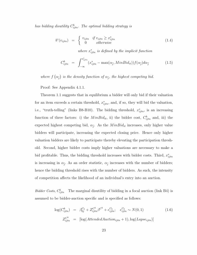
has bidding disutility Cbijtn. The optimal bidding strategy is
b∗(vijtn) =
vijtn if vijtn ≥ x∗ijtn0 otherwise
(1.4)
where x∗ijtn is defined by the implicit function
Cbijtn =
∫ x∗ijtn
−∞(x∗ijtn −max(αj,MinBidit))f(αj)dαj (1.5)
where f(αj)
is the density function of αj, the highest competing bid.
Proof: See Appendix 4.1.1.
Theorem 1.1 suggests that in equilibrium a bidder will only bid if their valuation
for an item exceeds a certain threshold, x∗ijtn, and, if so, they will bid the valuation,
i.e., “truth-telling” (links B8-B10). The bidding threshold, x∗ijtn, is an increasing
function of three factors: i) the MinBidit, ii) the bidder cost, Cbijtn and, iii) the
expected highest competing bid, αj. As the MinBidit increases, only higher value
bidders will participate, increasing the expected closing price. Hence only higher
valuation bidders are likely to participate thereby elevating the participation thresh-
old. Second, higher bidder costs imply higher valuations are necessary to make a
bid profitable. Thus, the bidding threshold increases with bidder costs. Third, x∗ijtn
is increasing in αj. As an order statistic, αj increases with the number of bidders;
hence the bidding threshold rises with the number of bidders. As such, the intensity
of competition affects the likelihood of an individual’s entry into an auction.
Bidder Costs, Cbijtn The marginal disutility of bidding in a focal auction (link B4) is
assumed to be bidder-auction specific and is specified as follows:
log(Cbijtn) = βCb0j + ZCb
ijtnβCb + eCbijtn; eCbijtn ∼ N(0, 1) (1.6)
ZCb
ijtn = [log(AttendedAuctionijtn + 1), log(Lapseijtn)]
23
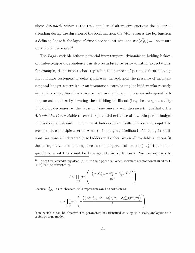
where AttendedAuction is the total number of alternative auctions the bidder is
attending during the duration of the focal auction; the “+1” ensures the log function
is defined; Lapse is the lapse of time since the last win; and var(eCbijtn) = 1 to ensure
identification of costs.16
The Lapse variable reflects potential inter-temporal dynamics in bidding behav-
ior. Inter-temporal dependence can also be induced by price or listing expectations.
For example, rising expectations regarding the number of potential future listings
might induce customers to delay purchases. In addition, the presence of an inter-
temporal budget constraint or an inventory constraint implies bidders who recently
win auctions may have less space or cash available to purchase on subsequent bid-
ding occasions, thereby lowering their bidding likelihood (i.e., the marginal utility
of bidding decreases as the lapse in time since a win decreases). Similarly, the
AttendedAuction variable reflects the potential existence of a within-period budget
or inventory constraint. In the event bidders have insufficient space or capital to
accommodate multiple auction wins, their marginal likelihood of bidding in addi-
tional auctions will decrease (else bidders will either bid on all available auctions (if
their marginal value of bidding exceeds the marginal cost) or none). βCb0j is a bidder-
specific constant to account for heterogeneity in bidder costs. We use log costs to
16 To see this, consider equation (4.46) in the Appendix. When variances are not constrained to 1,(4.46) can be rewritten as
L ∝∏ijtn
exp
−(log Cb
ijtn − βCb0j − ZCb
ijtnβCb
)2
2σ2
Because Cb
ijtn is not observed, this expression can be rewritten as
L ∝∏ijtn
exp
−((log Cb
ijtn)/σ − (βCb0j /σ)− ZCb
ijtn(βCb/σ))2
2
From which it can be observed the parameters are identified only up to a scale, analogous to aprobit or logit model.
24

ensure costs are positive. We assume βCb0j has the following hierarchical structure to
capture heterogeneity in costs across bidders.
βCb0j ∼ N(βCb0 , (φCb)−1
)(1.7)
βCb0 ∼ N(βCb
0 , σ20Cb
)
φCb ∼ Gamma(aCb0 , bCb0 )
On the surface, it may appear that bidder valuations and costs are not separately
identified, as a concurrent increase in both would yield the same bidder profits and
thus bidding behavior. Observations of positive bids reveal the bidder’s valuation,
which in turn helps to determine their cost. With costs known, together with our
parametric specification regarding the costs, it becomes possible to infer values in
auctions wherein bids are not observed (that is, a bidder decide not to bid). In
addition, costs have a common parametric specification across different items. For
those observations with the same covariate values for bidder costs, the variation
in bidder behavior across these items helps to identify bidder valuations because
differences in costs cannot explain differences in bidding behavior (as these costs are
constant across bidders in this case).
1.3.4 The First Stage – Seller’s Model
The seller chooses the optimal number of items to list in order to maximize their
expected return. We first derive the expected revenue a seller obtains from listing
an item (links S3 and S4 in Figure 1.2), and then use this revenue in conjunction
with seller costs (links S1 and S2) to derive the expected return for listing a specific
number of items (links S5-S7) and the optimal number of items to list (link S8).
25
Expected Revenue for Listing An Item
Seller Expected Revenue E(Rsitn|·) Without Secret Reserve Price For auctions without
secret reserve prices, the seller receives the second highest bid when there are at
least two bidders competing. When there is only one bidder, the seller receives the
minimum bid MinBidit. If there is no bidder, E(Rsitn|·) = 0. We condition the seller
revenue on each of these events, as discussed next.
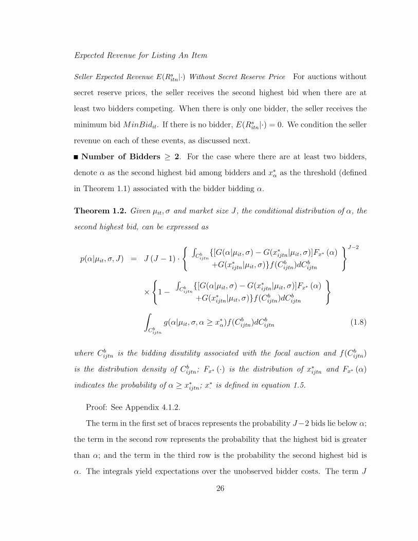
Number of Bidders ≥ 2. For the case where there are at least two bidders,
denote α as the second highest bid among bidders and x∗α as the threshold (defined
in Theorem 1.1) associated with the bidder bidding α.
Theorem 1.2. Given µit, σ and market size J , the conditional distribution of α, the
second highest bid, can be expressed as
p(α|µit, σ, J) = J (J − 1) ·
∫Cbijtn
[G(α|µit, σ)−G(x∗ijtn|µit, σ)]Fx∗ (α)
+G(x∗ijtn|µit, σ)f(Cbijtn)dC
bijtn
J−2
×
1−
∫Cbijtn
[G(α|µit, σ)−G(x∗ijtn|µit, σ)]Fx∗ (α)
+G(x∗ijtn|µit, σ)f(Cbijtn)dC
bijtn
∫Cbijtn
g(α|µit, σ, α ≥ x∗α)f(Cbijtn)dC
bijtn (1.8)
where Cbijtn is the bidding disutility associated with the focal auction and f(Cb
ijtn)
is the distribution density of Cbijtn; Fx∗ (·) is the distribution of x∗ijtn and Fx∗ (α)
indicates the probability of α ≥ x∗ijtn; x∗· is defined in equation 1.5.
Proof: See Appendix 4.1.2.
The term in the first set of braces represents the probability J−2 bids lie below α;
the term in the second row represents the probability that the highest bid is greater
than α; and the term in the third row is the probability the second highest bid is
α. The integrals yield expectations over the unobserved bidder costs. The term J
26

reflects the number of permutations in which α can be the second highest bidder.
Similarly, the term (J − 1) reflects the fact that any bidder among the (J − 1) bidders
(J bidders less the second highest one) can be the highest bidder.
Number of Bidders = 1. When there is only one bidder, just that bidder’s
valuation exceeds their threshold while the other J − 1 bidders do not. That yields
the probability of the seller earning MinBidit as the following
Pr(Rsitn = MinBidit) = J ·
∫Cbijtn
G(x∗ijtn|µit, σ)f(Cbijtn)dC
bijtnJ−1 (1.9)
×[1−∫Cbijtn
G(x∗ijtn|µit, σ)f(Cbijtn)dC
bijtn]
That is, for (J − 1) bidders, each has a valuation lower than the threshold, yielding
G(x∗ijtn|µit, σ). This is the term in the first set of brackets on the right hand side.
Given that Cbijtn is a random variable from the seller’s perspective, this term must be
integrated out. The second term pertains to the one bidder whose valuation exceeds
their threshold, leading to [1−∫Cbijtn
G(x∗ijtn|µit, σ)f(Cbijtn)dC
bijtn]. Moreover, as this
sole bidder is chosen from among J bidders, the final result needs to be multiplied
by J potential bidders that can have the highest bid (that is,(J1
)).
Combining equation 1.8 and 1.9 yields the conditional expected return of the
seller,
E(Rsitn|µit, σ, J) = E(α|µit, σ, J) +MinBidit · Pr(Rs
itn = MinBidit) (1.10)
=
∫ ∞
MinBidit
αp(α|µit, σ, J)dα+MinBidit · Pr(Rsitn = MinBidit).
Seller Expected Return With Secret Reserve Price The results developed in the case of
no secret reserve can be generalized as follows to the case of a secret reserve. First,
in the case of multiple bidders, if the second highest bid is lower than the secret
27

reserve, the seller keeps the item. Thus the return is zero. Second, in the one bidder
case, the seller retains the item because the winning bid must be MinBidit and is
therefore lower than the secret reserve.17 Hence, the expected return becomes
E(Rsitn|µit, σ, J) = E(α|µit, σ, J, α ≥ Reserveit) (1.11)
=
∫ ∞
Reserveit
αp(α|µit, σ, J)dα
The Seller Listing Decision
Seller Profits Prior to bidding, the seller must decide whether to list an item, and if
so, how many of the items to list.18 This decision is analogous to the seller choosing
the optimal supply of goods at a subgame level. We assume that seller i’s conditional
expected profit given listing qit units of item t is:19
πit(qit) = qit · (1− commission)E(Rsitn|·)− Cs
it(qit)− qit · feeit (1.12)
where commission is the commission rate charged by the auction house; feeit is the
unit listing fee paid to the auction site.20 Other than the listing fees and commissions
paid to the auction house, there exist acquisition or opportunity costs for an item.
The cost is assumed to depend on the item’s prevailing market value and the number
of units listed, qit. Owing to finite supply, as the seller endeavors to source more
units acquisition becomes more difficult. This leads to an increase in the marginal
17 Although the seller can still choose to sell the item if the realized final price is lower than thesecret reserve, we assume the seller assigns zero probability to such an event when calculating exante expected return.18 We also estimated a model wherein the minimum price decision is endogenous. The endogenousminimum price model yields a lower log marginal likelihood for the listing decision and bids (-21278.41 vs. -22150.82).19 Under the assumption that listing features are exogenous, a unique equilibrium is assured witha quasi-concave revenue function and a convex cost function.20 Given that commissions are tiered in our data, we compute commissions incumbent upon the auc-tion’s closing price. However, to facilitate exposition, we omit tier-specific commission subscriptsthroughout the paper.
28

opportunity cost of obtaining these items. Denote Csit(qit) as the total acquisition
cost for listing qit units. Increasing marginal costs imply that Csit(qit) is convex in qit.
Moreover, our specification implies that the expected revenue is quasi-concave in qit,
which is a necessary condition for a concave profit function and ensures an optimum
exists. The seller’s problem is to find the optimal qit that satisfies
qit = arg maxeqit πit(qit) (1.13)
i.e., any deviation from qit (i.e., selling fewer or more items) will not result in a higher
profit for the seller. As qit can include zero, the decision of whether to list, as what
number of items to list, is endogenous.
It is notable that observed variations in qit over the duration of the data leads
to estimated variations in the costs Csit over this duration. In turn, these variations
in acquisition costs inform how sellers’ listing behaviors vary with changes in costs.
In this fashion we can extrapolate how other costs (such as changes in fees) affect
listing behavior even if such changes are not observed in the data. Stated differently,
though there is no variation in fees over time from which to impute the seller listing
elasticity, we can use the link between costs and listings to assess how hypothetical
changes in fees affect listings.
Equation 1.13 indicates whether a given seller will list qit items. This decision
is affected by the number of competing sellers and participating buyers. As the
number of competing sellers increases, the total number of items listed to bidders
can increase. Yet equation 1.6 places a constraint on the number of auctions in which
a bidder can concurrently bid. In the presence of an increased number of items listed,
this constraint lowers the likelihood that any given seller will be able to sell their
items as an increase in the total listings leads to fewer bidders per auction listed. In
the presence of a fixed listing fee this lowers the expected return from listing an item.
Therefore, an increase in the number of sellers leads to a decrease in the expected
29

number of items listed by each seller. One implication of this is that the auction
house can manage this decrease in items listed per seller by lowering per item fees.
Likewise, the number of active buyers and their respective valuations affect the
seller’s listing decision. The expected return in equation 1.12 is a function of the
second highest bid, as noted in equation 1.10. The second highest bid is, in turn,
a function of the number of bidders J and their bidding thresholds x∗ as indicated
in equation 1.8. As more bidders become active (i.e., x∗ decreases – which could
occur if the mean of the valuation distribution increases) or the universe of bidders
becomes larger (J increases – for example, the bidding population become larger)
then the seller return increases and more sellers will list. In sum, the number of items
listed affects buyer participation and the buyer participation affects the number of
items listed. Hence, there is a structural link between seller and bidder behaviors.
Seller Acquisition Cost, Csit Given the foregoing concavity assumption, we specify the
prior distribution of seller i’s acquisition cost to be:
Csit = βCs0i BOOKV AL
βCs1it q
βCs2it + eCsqit (1.14)
We include a seller-specific constant term, βCs0i , to capture unobserved heterogeneity
in seller costs. eCsqit is an i.i.d. error term following normal distribution with mean 0
and variance θ−1 (the prior specifications for θ and other parameters are detailed in
Appendix 4.1.3). The stochastic terms are known by the seller itself but unobserved
by researchers. Delivery costs, which are unobserved, can affect both the average
seller costs βCs0i and per item costs βCs2 (Lewis et al., 2006). These costs, which are
unobserved, can affect both the average seller costs βCs0i and per item costs βCs2 .
30

We adopt the following hierarchical structure for the heterogenous constant term:
βCs0i ∼ N(βCs0 , (φCs)−1
)(1.15)
βCs0 ∼ N(βCs
0 , σ20Cs)
φCs ∼ Gamma(aCs0 , bCs0 )
Similar to the bidder cost, multiple observations of sellers across auctions enable
the identification of seller cost from valuation distribution (which is an important
component determining seller revenues). In particular, seller costs are identified
through the observed bids, bidder costs, and seller’s listing behavior across multiple
auctions.
1.4 Estimation
We adopt MCMC approach to estimate the model due to the flexibility of Bayesian
methods (Rossi et al., 1996). In particular, it enables us to readily accommodate
latent variables via data augmentation, including bidder valuations, bidder disutility
and seller profits. Moreover, the approach enables us to readily estimate a complex
model. In this section we define the likelihood and in the Appendix 4.1.3 we detail
the sampling chain and priors.
1.4.1 The Conditional Likelihood of Bidder Model
Given the threshold level x∗ijtn, the conditional likelihood of bidder j bidding on
auction itn is,
(pbidijtn|µit, σ,MinBidit, Cbijtn) = [g(bijt·|µit, σ)]I
bid
[g(v∗ijtn|µit, σ,MinBidit, Cbijtn)]
1−Ibid
(1.16)
where bijt· is the bidder’s revealed valuation from either a) the current auction n or
b) the bidder’s most recent bid on a like item (e.g., the same coin type) in a previous
31

auction; Ibid equals one if the bidder’s valuation has been revealed; v∗ijtn is a partially
latent valuation drawn from the valuation distribution if Ibid = 0. The first term
in (1.16) reflects the case where a bid is observed, and the likelihood of observing
bijt· on this instance is g(bijt·|·). The second term reflects the case where a bid is
not observed (Ibid = 0). In this case, the latent valuation v∗ijtn is obtained from the
distribution g(·|·) truncated at x∗ijtn, where x∗ijtn is defined in Theorem 1.1.
The product of equation 1.16 across ijtn gives the conditional likelihood of bidder
model,
Lbidder =∏i,j,t,n
(pbidijtn|·) (1.17)
1.4.2 The Conditional Likelihood of Seller Model
The decision regarding the number of items to list, qit, enters the likelihood as follows:
plistit (qobserved = qit|·) =∏
eqit 6=qitPrπit(qit) ≥ πit(qit 6= qit) (1.18)
That is, the estimated parameters should maximize the likelihood such that any
deviations from the observed qit can not result in extra profit. In practice, given the
fact that qit can assume an infinite number of values, it is impossible to calculate
πit(qit 6= qit) for all potential values of qit. Instead, we approximate the likelihood
by considering only those profits for a set of qit’s that are within an arbitrarily large
range around the observed qit. Given that the profit function is assumed to be
concave, any dramatic deviation of qit from the observed qit is unlikely to achieve a
higher profit. Therefore the probability of Prπit(qit) ≥ πit(qit 6= qit) approaches 1.
Hence, our approximation is not likely to be very restrictive.
The conditional likelihood of seller’s model is the product of plistit across i, t,
Lseller =∏i,t
plistit (qobserved = qit|·) (1.19)
32

Hence the conditional likelihood for the integrated bidder and seller model is
L = Lbidder · Lseller (1.20)
1.4.3 Augmented Full Posterior Distribution
By conditioning on the unobserved latent variables, v∗ijtn, πit and Cbijtn, the model
likelihood can be written as follows,
Laugmented|Ω (1.21)
=
∫Cbijtn
∫v∗ijtn
∫πit(qit)
∫πit(eqit)(L
bidder|v∗ijtnCbijtn)(L
seller|v∗ijtnCbijtn, πit(qit), πit(qit))
∏i,j,t,n
p(Cbijtn|ΩCb)
∏i,j,t,n
p(v∗ijtn|Ωv∗)
∏i,t
p(πit(qit)|Ωq)∏i,t,eqit
p(πit(qit)|Ωeq)dπit(qit)dπit(qit)dv∗ijtndCbijtn
where Lbidder is the bidder model likelihood from equation 1.17, Lseller is the seller
model likelihood from equation 1.19, Cbijtn is the latent bidder disutility from equation
1.6, v∗ijtn is the latent bidder value from equation 1.1, πit((qit)|·) and πit((qit)|·) are
latent profits from equation 1.12 and Ω = ΩCb ,Ωv∗ ,Ωq,Ωeq are the model parame-
ters. As the latent variables are unobserved, we must integrate over these variables
to compute the likelihood. We perform this integration via an MCMC approach
using data augmentation. One advantage of this approach is that it yields estimates
for the distribution of the latent variables which become useful in our policy analysis
(for example, we can estimate the unobserved listing costs for each seller and valu-
ations of each bidder). Another advantage of this approach is that it facilitates the
integration.
The augmented full posterior can then be constructed by multiplying the likeli-
hood by the prior,
p(Ω|Laugmented) ∝ (Laugmented|Ω) ∗ p(Ω)
33
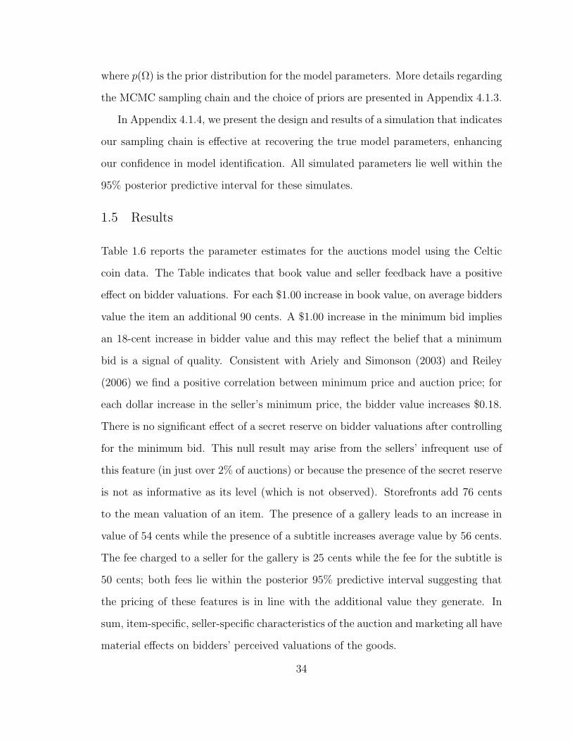
where p(Ω) is the prior distribution for the model parameters. More details regarding
the MCMC sampling chain and the choice of priors are presented in Appendix 4.1.3.
In Appendix 4.1.4, we present the design and results of a simulation that indicates
our sampling chain is effective at recovering the true model parameters, enhancing
our confidence in model identification. All simulated parameters lie well within the
95% posterior predictive interval for these simulates.
1.5 Results
Table 1.6 reports the parameter estimates for the auctions model using the Celtic
coin data. The Table indicates that book value and seller feedback have a positive
effect on bidder valuations. For each $1.00 increase in book value, on average bidders
value the item an additional 90 cents. A $1.00 increase in the minimum bid implies
an 18-cent increase in bidder value and this may reflect the belief that a minimum
bid is a signal of quality. Consistent with Ariely and Simonson (2003) and Reiley
(2006) we find a positive correlation between minimum price and auction price; for
each dollar increase in the seller’s minimum price, the bidder value increases $0.18.
There is no significant effect of a secret reserve on bidder valuations after controlling
for the minimum bid. This null result may arise from the sellers’ infrequent use of
this feature (in just over 2% of auctions) or because the presence of the secret reserve
is not as informative as its level (which is not observed). Storefronts add 76 cents
to the mean valuation of an item. The presence of a gallery leads to an increase in
value of 54 cents while the presence of a subtitle increases average value by 56 cents.
The fee charged to a seller for the gallery is 25 cents while the fee for the subtitle is
50 cents; both fees lie within the posterior 95% predictive interval suggesting that
the pricing of these features is in line with the additional value they generate. In
sum, item-specific, seller-specific characteristics of the auction and marketing all have
material effects on bidders’ perceived valuations of the goods.
34

Table 1.6: Posterior Means and Standard Deviations of Model Parameters
Median 95% IntervalValuation Distributionµ
Constant 0.59* (0.31, 0.82)Book Value 0.90* (0.89, 0.92)(Seller Feedback)/100 0.03* (0.02, 0.04)Minimum Bid 0.18* (0.15, 0.21)Secret Reserve Dummy 0.28 (-0.16, 0.99)Store Dummy 0.76* (0.32, 1.21)Gallery Picture Dummy 0.54* (0.04, 0.79)Subtitle Dummy 0.56* (0.02, 2.21)
σConstant 4.00* (3.84, 4.41)
Bidder DisutilityNumber Auctions Attended 0.79* (0.70, 0.95)Lapse Since Last Winning -0.31* (-0.34, -0.28)Mean Individual Constant 1.68* (1.50, 1.78)
Seller Acquisition CostBook Value 0.86* (0.65, 1.07)Number of Listings 1.27* (1.02, 1.55)Cost Error Variance 0.95* (0.65, 1.19)Mean Individual Constant 1.05* (0.98, 1.13)
Log Marginal Likelihood -21278.41
The number of auctions attended increases one’s bidding disutility, suggesting de-
creasing marginal returns for auctions. Meanwhile, consistent with an inter-temporal
budget constraint, we find that a bidder’s likelihood of attending new auctions de-
creases if they won recently (or, alternatively, there are decreasing marginal returns
for acquiring an additional item). A significant positive constant cost exists. The
constant implies a fixed bidding disutility in the neighborhood of $5.37. Since we use
a log-log specification for bidder disutility, the parameters for AttendedAuction and
Lapse can be interpreted as elasticities or sensitivities. Hence the bidding disutility
elasticities for concurrent auctions attended and lapse of time are around 0.79 and
−0.31, respectively.
35

Figure 1.4: Observed Bids Vs. Simulated Bids
Acquisition opportunity costs for a seller increase with an item’s book value.
In particular, given the log-log specification, one can interpret the parameters as
elasticities. For a 1 percent increase in the book value, there is an impact on the
seller’s total cost in the amount of 0.86 percent. Further, the elasticity of seller cost
for the number of listings is 1.27. The mean of the seller-specific constant term is
1.05. As the constant term serves as a scaling factor in our formulation of seller costs,
the finding that this term is close to one suggests the scaling effect is immaterial. In
other words, seller acquisition costs are largely determined by per item costs and the
opportunity cost for multiple listings.
To illustrate the fit of our model, we simulate bid values within sample based
on our estimates and data. We then compare the observed bid/book ratios with
the simulated ratios. Figure 1.4 shows the comparison between the two variable
distributions. The model fits the mean bid to book ratio very well (Observed =
36

0.48, Simulated = 0.48). The median is also comparable (0.31 vs. 0.39). Overall,
the fit seems good, suggesting our model specification captures the observed bidding
behaviors well.
Of note, we contrast the full model to one wherein we model only bidder behav-
ior. The bidder-model parameter estimates are virtually identical to those obtained
using the full model though the full model yields better predictions regarding bidder
behavior, potentially suggesting gains in efficiency arising from joint estimation (the
log-marginal likelihood for bidders in the joint model is −20062.5 vs. −20265.2 in the
buyer only model). We speculate that the similarity in bidder parameter estimates
across the bidder only and bidder-seller models reflects independence in errors across
the bidder and lister models; this finding would be less likely to obtain in the face of
omitted variables that could induce correlated errors. Though our results indicate
joint estimation is more likely an issue of efficiency than bias, it is important to note
that estimates pertaining to seller behavior are requisite for engaging the policy sim-
ulations that underpin the goals of this paper. Hence our research could not proceed
without the seller model.
1.6 Managerial Implications
Whereas the parameter estimates are informative about bidder and seller behavior,
they offer little explicit guidance to the auction house regarding its marketing strat-
egy. We consider three strategic implications: a manipulation of auction house fees
(which is informative about optimal pricing), the attrition of a customer (which is
informative about customer value), and the effect of seller characteristics on auction
house revenues (which places a value on a seller’s reputational capital).
37

1.6.1 Auction House Pricing
Pricing Elasticity and Optimal Pricing
Using the model estimates, one can assess the effect of the auction house pricing
strategy on the market equilibrium number of listings, bids and closing prices in the
considered category.21 As noted above, we can infer the price-demand relationship
even in the absence of any historic variation in fees because the structural model is
informative about the latent bidder and seller costs and the bidder valuations. The
price-demand relationship enables us to infer how a change in auction house fees
affects seller profits, hence the seller listings and the resulting bidder demand. With
information on the number and closing price of auctions, the auction house can assess
how a fee change affects its revenue (which is equal to the total merchandise volume
in the market times the percent commission plus the total number of listed items
times the listing fee per item). In Table 1.7 we compute auction fee price elasticities
by simulating the effect of a 1% decrease in current listing fees and commissions on
profits.22
Table 1.7 indicates that a decrease in fees improves seller profits, leading to more
listings and more gross volume sold on the site.23 However, the effect is much larger
for commissions than listing fees. As a result, the overall increase in volume at
21 Note that our model assumes that buyers and seller behave optimally while our simulationpresumes the auction house does not. Prima facie, this seems inconsistent. However, there existsome differences between these parties. First and foremost, the firm has indicated directly to usthat its pricing does not follow an elasticity-based approach but that it is more heuristic based.Hence they are interested in using elasticity based pricing to inform their decisions, which is akey goal of this exercise. Second, buyers and sellers face repeated observations and play auctionsover many occasions. This suggests the potential for learning and feedback, as such, the “as if”optimality assumption may be reasonable (Amaldoss and Jain, 2005). In contrast, little pricevariation exists for the auction house making it difficult to learn.22 The auction house utilizes a tiered commission system. To protect the confidentiality of the datasupplier, we do not reveal the actual commissions. To compute the elasticities, we decrease thecommission at each level by 1%. Likewise we reduce the listing fees by 1%.23 We do not report actual revenues to protect the confidentiality of the data provider. However,the actual revenue lies within the 95% posterior predictive interval for estimated revenues.
38

Table 1.7: Fee and Commission Price Elasticities
Percentage Change 1% Decrease in Commissions 1% Decrease in Listing FeesSeller Profit 3.90 (1.67, 5.90) 1.93 (0, 4.94)Number of Auctions 2.04 (0, 8.95) 0.68 (0, 1.99)Auction Website Revenue 0.86 (0.09, 1.85) -0.08 (-0.11, -0.03)
the auction site arising from a commission decrease generates enough total revenue
to offset the reduction in per item commissions. In contrast, the increased volume
arising from reduced per item listing fees does not offset the loss in the per item
listing fee. All 95% posterior predictive intervals for these fee elasticities exclude
zero. Accordingly, we would recommend that the auction house shift its fees for this
category from commissions to listing fees by reducing the commissions and increasing
the listing fees. At a minimum we would recommend that they refrain from raising
commissions further by raising listing fees instead.
This recommendation can in part be explained by noting how different fee types
affect sellers. Per item fees are an example of a uniform pricing strategy whereas
commissions tend to disproportionately affect higher value items. As a result, a
decrease in commissions disproportionately affects high value sellers relative to a
decrease in fees. Simulating the effect of a 2 point decrease in commissions, we ob-
serve more high book value items listed and high feedback sellers listing more items
relative to the case wherein per item fees are decreased. As higher book values and
reputations lead to increased item valuations, a reduction in commissions dispro-
portionately affects these groups thereby leading to an increase in high valuation
listings. Given that these high valuation items generate higher profits for the seller,
a small reduction in commissions can lead to a considerable increase in seller profits
for such items and a concurrent increase in listings. We note that these effects are
likely to be amplified in categories wherein valuations and feedback scores assume
39

greater importance, such as art. To further assess the degree to which listing fees
should be increased and commissions reduced for the considered category, we create
a 9 by 6 grid of alternative commission and listing fee structures and estimate the
house revenues associated with each fee combination. Table 1.8 reports the result of
this analysis.
Table 1.8: Revenue Percentage Changes with Alternative Pricing Schedules
Commissions (points)\ Fees (%) 0 5 10 15 20 250 0 0.37 0.63 0.96 0.76 0.13
-0.25 1.04 1.48 1.74 1.77 1.21 0.30-0.50 1.11 1.61 1.84 2.03 1.37 1.30-0.75 1.19 1.87 2.19 2.89 2.66 1.76-1.00 1.16 1.77 1.97 2.87 2.49 1.65-1.25 1.12 1.38 1.68 1.90 1.61 1.33-1.50 1.01 1.19 1.48 1.73 1.53 1.07-1.75 0.97 1.18 1.48 1.71 1.52 0.81-2.00 0.31 0.81 0.93 1.39 0.87 0.39
The upper left corner of Table 1.8 reflects the current level of listing fees and
commissions. Each subsequent row indicates the effect of a one quarter point decrease
in commissions. Thus, the last row indicates a two point decrease in commissions.24
Each subsequent column from left to right indicates the effect of a 5% increase in the
listing fee. Thus, the last column indicates a 25% increase in listing fees from the
current level. The cells in Table 1.8 report the percentage change in auction house
revenue for each combination of commission and listing fees; in general, revenues
increase with lower commissions and higher fees. The maximum revenue increase
of roughly 3% is associated with a 0.75 point reduction in commissions and a 15%
increase in listing fees. Even were the auction house not to decrease commissions, it
24 We base the two point decrease upon the highest commission rate (which is associated with thelowest tier of closing prices). We then translate this point decrease to a percentage and apply it tothe other pricing tiers.
40

is possible to increase revenues by nearly 1% with a 15% increase in listing fees. To
the extent similar increases could be realized across categories, a 3% increase could
prove quite considerable.
Price Customization
Recently, Zhang and Wedel (2008) have proposed that the pricing customization
across customers enhances profits in the context of frequently purchased grocery
goods. We therefore seek to assess whether the result is similar in the context of
auctions. One reason to believe customization may be efficacious is the relatively
high dispersion in the value of items listed for sale in the auction context (book
values range from $3 to $675). Sellers of high value listings (defined as those items
with greater value than the median Book Value) stand to gain more from changes to
commissions whereas sellers of low value items stand to gain more from changes in per
item listing fees. To explore whether we can improve upon the pricing strategies in
Table 1.8, we proceed as follows. Instead of increasing fees and lowering commissions
to all sellers, we increase fees and lower commissions only for high value sellers. Given
sellers of high value items are more sensitive to commissions and less sensitive to fees,
targeting a price change to these sellers could prove profitable. Table 1.9 reports this
analysis.
Comparing the first columns of Table 1.8 with those in Table 1.9, we observe that
a 0.75 point decrease in commissions (and no change in per item fees) targeted to
only the high item value sellers yields a nearly 3.0% revenue increase in a customized
setting but only a 1.2% increase in the uniform pricing setting. Not only does this
triple the revenue gain observed in the non-targeted pricing setting, it exceeds the
maximum potential return of 2.89% when prices are not customized. Therefore,
targeting commissions seems to have a material effect on revenues. Contrasting the
first rows of Table 1.8 to those in Table 1.9 yields a comparison between raising per
41

Table 1.9: Revenue Effects with Targeting of Commissions and Fees
Commissions (points)\Fees (%) 0 5 10 15 20 250 0 0.34 0.82 0.99 0.73 0.69
-0.25 1.00 1.37 1.70 1.98 1.26 1.28-0.50 2.09 2.59 3.47 3.67 2.57 2.37-0.75 2.93 3.13 3.82 3.91 2.96 2.47-1.00 2.92 3.07 3.80 3.84 2.59 2.28-1.25 2.21 2.49 2.62 2.31 2.19 2.00-1.50 1.02 1.11 1.80 2.02 1.78 1.76-1.75 0.91 1.03 1.73 1.81 1.91 1.16-2.00 0.22 0.54 1.07 1.57 1.04 0.43
item listing fees to all sellers with only raising fees to high value sellers (as low value
sellers are presumably more sensitive to fees). As the cells are comparable across
the two Tables, we conclude that there is little benefit to targeting fees relative
to targeting commissions. Finally, Table 1.9 suggests the maximum return of the
proposed customized strategy (obtained with a 0.75 point decrease in commission
and a 15% increase in fee to high value sellers,) to be 3.91% compared to 2.89% from
the blanket strategy. Thus, the potential gain arising from targeted pricing is about
35%. These numbers are in line with the findings of Zhang and Wedel (2008).
In sum, the joint model of bidder and seller behavior enables us to develop pricing
prescriptions even in absence of any historical pricing variation. Given the total vol-
ume transacted in the area of Internet auctions, the pricing problem is an important
one and the proposed model represents an initial step towards addressing this prob-
lem. In principle, other policy simulations are possible with our model, including
an assessment of how a change in auction rules away from sealed bid second price
auctions would affect auction house revenue.
42

1.6.2 Customer Value in a Two-sided Market
Valuing customers has seen increased research attention in marketing in recent years
(Kamakura et al., 2005). Firms seek to assess customer profitability in order to deter-
mine how much to invest in a given customer (for retention or acquisition), whether
to divest an unprofitable customer and for firm valuation. Yet the customer valuation
literature focuses on customer valuation in contexts where one customer’s presence
does not affect another. Valuing customers in two-sided markets is problematic be-
cause of the interaction between bidders and sellers. Exacerbating this consideration
in the context of auctions is the role of competition in customer valuation. Should a
seller attrite, the supply of auctions decreases. Given price increases are permanent,
this has two enduring effects: i) fewer items listed leads to increased competition on
the part of bidders for the remaining items, thereby driving up prices resulting in
higher per-auction commissions for the auction house and ii) higher prices paid by
buyers and lesser competition encourages the remaining sellers to list some additional
items which will also generate revenue for the auction house. These factors, which
we denote indirect value effects, will offset the initial revenue lost from a departing
seller (denoted direct value effects) and these indirect effects could be considerable.
A similar categorization applies on the bidder side. When one buyer departs the
system, others that remain will bid for the items thereby offsetting this loss to some
degree. However, softer competition among bidders could also lead to lower prices
and therefore fewer items listed on the part of sellers. Thus, the direct value effect
for a buyer in terms of auction revenue is offset to some degree by the presence of
other bidders in the system provided this does not induce too many sellers to depart.
In the absence of a model that captures competitive interactions, it is unclear
how to value customers. The most commonly used practice is to use the direct
effect to measure customer value. However, this approach overstates the value of
43

a customer by ignoring competition. Our solution to this problem is to conduct a
policy experiment wherein a particular buyer or seller is excluded from the system
and compute the change in the equilibrium number of listings and closing prices
of those listings over the duration of the data. By comparing the new equilibrium
to the original, we can compute the short-term value of a customer to the auction
house. In doing so, we abstract away from long-term dynamics such as the growth
(diffusion) of bidders and sellers (Gupta et al., 2006). It is therefore important to
delineate between our short-term measure of customer value (as in our approach)
and the more forward-looking lifetime value metrics often used in marketing (Gupta
et al., 2006; Kamakura et al., 2005). Table 1.10 reports the result of a simulation
wherein the largest buyer and seller, respectively, attrite and the resulting loss in
fees to the auction house.
Table 1.10: The Value of the Largest Customer
Seller BuyerDollars Percent Dollars Percent
Direct Value $127 100% $26 100%Indirect Value −$30 24% −$21 81%Total Value $97 76% $5 19%
The first row of Table 1.10 presents the direct value effects or the revenue of the
auctions in which the customer participates, reflecting the total fees arising from the
auctions in which the largest seller and buyer transact (a commonly used metric for
valuing a customer in a two-sided market). The third row reports the equilibrium
revenue realized by the auction house when the customer attrites as computed by
our model (we call this the total effect as it is the sum of the direct effect plus the
indirect and opposite effect arising from competition). The second row reports the
difference between the direct effect and the total effect (i.e., the indirect effect). We
also compute the relative percentage of the total effect that arises from the direct
44

and indirect effects. For example, the direct effect of the largest seller on auction
house revenues is $127. The revenue realized by the auction house were this seller to
attrite is $97 (the total effect). Thus, the direct effects overstate the total revenue loss
by $30, or nearly a third ($30/$97). Given that competition does not offset most
of the loss, we conclude that products sold by this vendor in this market are not
altogether highly substitutable with the other products being auctioned. A rather
different conclusion is realized on the buyer side where the largest buyer generates
$26 in direct revenue but only $5 in total revenue, suggesting the indirect effects to
be $21. When this buyer leaves the market, others fill the void. Accordingly, the
direct effects overstate the total effect by over 400%.
As noted above, indirect effects manifest as a change in equilibrium prices and
supply. We can apportion the indirect effects across prices and supply in order to
ascertain which effect is greater. This decomposition yields insights into whether the
largest customer is more likely to affect listings (driven by seller behavior) or the
closing price per listing (driven by bidder behavior). Let N0 denote the number of
closing auctions listed by competing sellers prior to attrition of the largest seller and
p0 denote the N0 ∗ 1 vector of unit revenues (commission plus listing fees) of those
auctions. Similarly, we denote the number of auctions and vector of unit revenues
after the largest seller attrites as Ns and ps. Using this notation, we compute i) the
indirect effects arising solely from a change in unit revenues holding the number of
auctions fixed, (Ns∑k=1
psk−Ns∑k=1
p0k) and ii) the expected change in revenue arising from
a change in the number of auctions holding the unit revenues fixed, (Ns∑k=1
p0k−N0∑k=1
p0k).
We use a similar decomposition to assess the effect of buyer attrition. Table 1.11
presents the results of this analysis.
Columns 2 and 3 report the results of this analysis for the attrition of the largest
45

Table 1.11: Indirect Value Due to Listings and Prices
Seller BuyerValue Percent Value Percent
Indirect Value $30 100% $21 100%Effect Due to Adjustment in Listings $12 39% $12 57%Effect Due to Adjustment in Unit Revenues $18 61% $9 43%
seller and columns 4 and 5 report the analogous results for the attrition of the largest
buyer. Of the $30 indirect competitive effects that offset the total effect of the largest
seller’s attrition, about 2/5 ($12) of the competitive effects are due to other sellers
listing more items and about 3/5 ($18) of the competitive effect is due to higher
prices that arise from bidders bidding on fewer goods on the market. Thus, seller
attrition plays a major role on both competitor behavior (items listed) and bidder
behavior (bids).
With regard to the departure of the largest buyer, about 2/5 ($9) of the indirect
effects can be attributed to the unit revenue change and 3/5 ($12) can be accounted
by changes of number of auctions. Although the biggest bidder attrites, other bidders
step in to fill the void and generate $21 to largely offset the $26 loss. Overall we
conclude that, under a two-sided market such as online auction, using direct revenue
as the metric may overstate a customer’s value considerably. To accurately measure
the value of a customer, a firm needs to take into account the network externalities
caused by the customer.
1.6.3 Elasticities of Seller Feedback Scores
As noted in the literature on signalling game, seller feedback should play a role
in transmitting the quality of their product leading to increased bids (Cabral and
Hortacsu, 2006). Table 1.6 confirms this proposition suggesting an increase of 100
in the seller feedback score leads to an average increase in customer valuation of
46
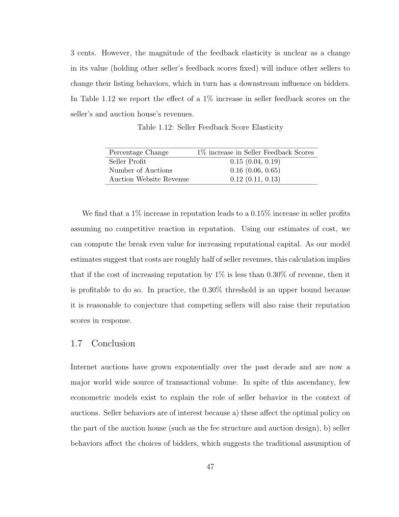
3 cents. However, the magnitude of the feedback elasticity is unclear as a change
in its value (holding other seller’s feedback scores fixed) will induce other sellers to
change their listing behaviors, which in turn has a downstream influence on bidders.
In Table 1.12 we report the effect of a 1% increase in seller feedback scores on the
seller’s and auction house’s revenues.
Table 1.12: Seller Feedback Score Elasticity
Percentage Change 1% increase in Seller Feedback ScoresSeller Profit 0.15 (0.04, 0.19)Number of Auctions 0.16 (0.06, 0.65)Auction Website Revenue 0.12 (0.11, 0.13)
We find that a 1% increase in reputation leads to a 0.15% increase in seller profits
assuming no competitive reaction in reputation. Using our estimates of cost, we
can compute the break even value for increasing reputational capital. As our model
estimates suggest that costs are roughly half of seller revenues, this calculation implies
that if the cost of increasing reputation by 1% is less than 0.30% of revenue, then it
is profitable to do so. In practice, the 0.30% threshold is an upper bound because
it is reasonable to conjecture that competing sellers will also raise their reputation
scores in response.
1.7 Conclusion
Internet auctions have grown exponentially over the past decade and are now a
major world wide source of transactional volume. In spite of this ascendancy, few
econometric models exist to explain the role of seller behavior in the context of
auctions. Seller behaviors are of interest because a) these affect the optimal policy on
the part of the auction house (such as the fee structure and auction design), b) seller
behaviors affect the choices of bidders, which suggests the traditional assumption of
47
exogenous seller behavior in the empirical IO literature may be questionable, and
c) seller behavior is of interest in its own right (in assessing customer value, for
example).
We redress this consideration via a structural model of seller and bidder behaviors
across auctions. We posit sellers will list if the return from doing so exceeds their
respective costs. Likewise, we presume the bidders will bid if the expected return
from doing so exceeds their respective costs. An important component of the model
is its integration of bidder and seller behavior. Sellers, when deciding to list, must
consider the bids likely to materialize if they list and also the potential of competitive
listings. Likewise, bidders must consider the number of auctions across which they
can bid. In this fashion, the behaviors of the two groups are linked. This linkage
exemplifies a two-sided market wherein bidders and sellers interact on a common
platform (Rochet and Tirole, 2006) and extends structural models of auctions into
this domain.
Accordingly, we develop an empirical structural model which rationalizes bidder
and seller behavior under the auction context. We estimate this model using six
months of auction data for Celtic coins provided by an auction house. The data are
consistent with an independent private value auction. We use MCMC techniques
to estimate the costs and valuations that would be consistent with the bidding and
listing behavior observed in the data. Once these are known, it becomes possible to
assess the role of fees on equilibrium listings. That is, as fees rise, seller profits fall
and they are less likely to list. Bidders, faced with fewer auctions, will increase their
bids to win. The net effect can be determined in this fashion.
The estimates from our empirical model indicate that item characteristics (such
as its book value), seller characteristics (their feedback scores), and marketing tools
(minimum bid, the use of a store front, and additional item information revealed by
a subtitle and a picture) have significant impacts on bidder valuations and thus their
48
bids. We further develop insights into bidder and seller costs and valuations, such
as the finding that a 1% increase in book value on average increases seller costs by
0.86%.
Using these results, our policy experiment indicates that an increase in listing fees
will increase auction house revenues while an increase in commissions will decrease
them. By searching over a grid of values in the neighborhood of its current fees, we
find that the change in fees and commissions can bring an increase of nearly 3% in
auction house revenues for the Celtic coin category. The intuition behind this result
is that fees exemplify a uniform pricing policy whereas commissions are a form of
high value pricing discrimination. As such, a decrease in commissions has a large
effect on the profitability of high valuation items (such as those with a high book
value and listed by high reputation sellers) leading to a large increase in listings for
such items. Accordingly, we expect our finding that pricing should be reallocated
toward fixed fees to be amplified in categories with more high valuations items and
attenuated in categories with lower valuation items. We build further upon this
intuition by considering a targeted pricing strategy wherein high value users face
lower commissions and higher per item fees than low value users. We find that
customized pricing can increase revenues by 35% over the uniform pricing solution.
The approach developed herein is also useful for assessing short-term customer
value in two sided markets. Customer value is relevant to firms seeking to assess
how much to invest in retaining or acquiring customers and, to date, this literature
has been silent on the value of customers in the context of two-sided markets. The
primary information available to value a customer (such as a seller) is the revenue
that customer generates for a firm. However, such a valuation fails to account for
competitive effects such as the tendency of bidders to switch to other sellers when
a seller attrites and the tendency of other sellers to list more items. In general, we
find approaches that ignore such indirect effects to overstate customer value of the
49

seller by nearly a third and the value of a buyer by over 400%. We further apportion
these indirect seller effects into an increase in the number of listings by competing
sellers who seek to capitalize on the departure of competition and the increase in
prices arising from stiffer bidder competition for the remaining items. We find these
effects to be roughly equal.
The complexity of the problem we consider necessitates some simplifications,
which also represent both limits and future research opportunities. In particular,
we approximate bidding dynamics using lagged purchases in the cost function to
capture inter-temporal dynamics and multi-auction bidding that may be induced
by an inter-temporal multi-item budget constraint or price expectations. A more
complete specification regarding the dynamics might yield some novel insights. Fur-
ther research is therefore warranted. Second, consistent with our data, our model
utilizes the private value assumption to simplify the analysis. An extension to the
common value setting would yield interesting insights regarding interactions among
bidders. Third, we do not consider competition between auction houses. We believe
this is a reasonable approach, as fees constitute a relatively small component of the
overall cost of listing items in this category and because the large number of bidders
and sellers on this site make it less likely that competing sites would be attractive
alternatives to sellers. Nonetheless, inter-site competition is widely unaddressed in
the literature and represents an important direction for future analysis. Fourth, we
presume the auction house is not strategic in its price setting behavior. Though this
assumption is predicated on conversations with price setters at this organization,
many firms (e.g., Google and Yahoo!) are strategic in their use of pricing mecha-
nisms and it would be interesting to address this issue. Fifth, we consider listing
features to be exogenous. It is unlikely that endogenizing these variables will yield
a unique equilibrium, so it is unclear whether relaxing this restriction will be useful
for policy analysis. Moreover, given the number of potential combinations of these
50

features, it is not clear that it is possible to solve for all of them. Yet these features
represent a source of revenue to the auction house, and the problem of how to price
these is another area of importance to consider; recent advances in combinatorial op-
timization could prove fruitful here. In sum, we believe that the combination of the
material economic importance of auctions and the large array of remaining problems
for consideration suggests this is a rich area for future research. We hope our initial
foray into the problem of bidder and seller networks in the context of auctions will
lead to further research in this domain.
51
2
A Dynamic Model of Sponsored Search Advertising
2.1 Introduction
Sponsored search is one of the largest and fastest growing advertising channels. In
January of 2009 alone, Internet users conducted 13.5B searches using the top 5 Amer-
ican search engines compared to 10.5B in the previous January, indicating a robust
29% year over year increase.1 In the United States, annual expenditures on sponsored
search advertising increased 28% to $8.9B in 2007, and the number of firms using
sponsored search advertising rose from 29% to 41%.2 Moreover, advertising expendi-
tures on sponsored search is forecast to grow to $25B by 2012.3 By contrast, overall
2007 television advertising spending in the United States is estimated to be $62B,
an increase of only 0.7% from the preceding year.4 Hence, search engine marketing
is becoming a central component of the promotional mix in many organizations.
1 “January 2009 U.S. Search Engine Rankings,” comScore, Inc. (http://ir.comscore.com/releasedetail.cfm?ReleaseID=366442). “January 2008 U.S. Search Engine Rankings,” com-Score, Inc. (http://www.comscore.com/press/release.asp?press=2068).
2 “US Paid Search Forecast, 2007 to 2012,” Jupiter Research, 2007.3 “US Interactive Marketing Forecast, 2007 to 2012,” Forrestor Research, 2007.4 “Insider’s Report,” 2007, McCann WorldGroup, Inc.; http://www.tns-mi.com/news/
01082007.htm
52

The growth of this new medium can be ascribed to several factors. First, the
increasing popularity of search engine sites relative to other media among consumers
affords a greater advertising reach. In addition to searches on large general search
engines such as Google.com, MSN.com, and Yahoo.com, search is also widespread
on more focused ones (dealtime.com searches Internet stores, kayak.com searches
travel products, addall.com searches books, etc.). The broad reach of search can be
ascribed to the complexity of wading through an estimated 155 million sites to return
relevant results in response to users’ search queries.5 By comparison, a top rated TV
show such as “Desperate Housewives” only has about 25M viewers (IRI, 2007); and
the growing popularity of DVR services offered by TiVo and cable companies have
and will further decrease the audience base of traditional TV advertising. Second,
more and more consumers use the Internet for their transactions (Ansari et al.,
2008), and Internet search is an especially efficient way to promote online channels.
For example, Qiu et al. (2005) estimate that more than 13.6% of the web traffic is
affected by search engines. Third, search advertising often targets consumers who
are actively seeking information related to the advertisers’ products. For example,
a search of “sedan” and “automotive dealer” might signal an active purchase state.
As a result of these various factors, Jupiter Research reports that 82% of advertisers
were satisfied or extremely satisfied with search marketing ROI in 2006 and 65%
planned to increase search spending in 2007.6
Given the increasing ubiquity of sponsored search advertising, the topic has seen
substantially increased attention in marketing as of late (Ghose and Yang, 2007;
Rutz and Bucklin, 2007; Rutz and Bucklin, 2008; Goldfarb and Tucker, 2008). These
recent advances focus upon the efficacy of an advertiser campaign. To date, empirical
5 “January 2008 Web Server Survey,” Netcraft Company (http://news.netcraft.com/archives/2008/01/28/january_2008_web_server_survey.html).
6 “US Paid Search Forecast, 2007 to 2012,” Jupiter Research, 2007.
53
research on keyword search has been largely silent on the perspective of the search
engine, the competition between advertisers, and the behavior of the searcher. Given
that the search engine interacts with advertisers and searchers to determine the
price and consumer welfare of the advertising medium (and hence its efficacy), our
objective is to broaden this stream of research to incorporate the role of all three
agents: the search engine, the advertisers, and the searchers. This exercise enables
us to determine the role of search engine marketing strategy on the behavior of
advertisers and consumers as well as the attendant implications for search engine
revenues. Our key contributions are, accordingly, as follows:
1. From a theoretical perspective, we conceptualize and develop an integrated
model of web searcher, advertiser and search engine behavior. To our knowl-
edge, this is the first empirical paper focusing on the marketing strategy of
the search engine. Much like Yao and Mela (2008), we construct a model of
a two-sided network in an auction context. One side of the network includes
the searchers who generate revenue for the advertiser. On the other side of
the two-sided network are advertisers whose bidding behavior determines the
revenue of the search engine. In the middle lies the search engine. The goal
of the search engine is to price consumer information, set auction mechanisms,
and design webpages to elucidate product information so as to maximize its
profits. Some key insights from this model include:
• Advertisers in our application have an average value per click of $0.27.
Given that the average price of software products advertised on the site
in our data is about $22, this implies these advertisers expect about 1.2%
(i.e., $0.27/$22) of clicks will lead to a purchase. This is consistent with
the industry average of 1-2% reported by GameDaily.com, suggesting good
face validity for our model.
54

• In addition, we find considerable heterogeneity in consumer response to
sponsored search advertising. Frequent link clickers, who represent 10%
of the population but 90% of the clicks, tend to be more sensitive to slot
order – in part because slot position can signal product quality. These
insights represent central inputs into our policy simulations alluded to
below.
2. From a substantive point of view, we offer concrete marketing policy recom-
mendations to the search engine. In particular, the two-sided network model
of keyword search we consider allows us to address the effect of the following
policy simulations (and would enable us to address many others) on auction
house and advertiser profits as well as consumer welfare:
• Search Tools. Many search engines, especially specialized ones such as
Shopping.com, provide users options to sort/filter search results using
certain criteria such as product prices. On one hand, the search tools
may mitigate the desirability of bidding for advertisements because these
tools can remove less relevant advertisements. This would tend to lower
search engine revenues. On the other hand, these tools can also attract
more users to the site leading to a potential increase in advertising ex-
posures and searchers. This would increase revenues. The trade-off leads
to the question of how search tools impact consumer searching behavior,
firms’ advertising decisions, and search engine profits. Our analysis in-
dicates that negative consumer effects on search engine profits (−6.4%)
outweigh the corresponding positive advertiser effects on search engine
profits (2.7%) and that overall the sort/filter options enhance platform
profits by 3.7%. Consistent with this result, there is a corresponding loss
in consumer welfare of 5.6% and an attendant increase in advertiser profits
55

of 4.1%.
• Segmentation and Targeting. Most search engines auction keywords across
all market segments. However, it is possible to auction keywords by seg-
ment. This targeting tends to reduce competition between advertisers
within segments as markets are sliced more narrowly, leading to lower
bids and hence lower potential revenues for the search engine. Yet tar-
geting also enhances the efficiency of advertising, which tends to increase
advertiser bids. Overall, we find that the latter effect dominates (2.2%)
the former effect (−0.8%) and that search engine revenue increases 1.4%
by purveying keywords by consumer market segments. Moreover, we find
advertiser profits improve by 11% (from reduced competition in bidding
and more efficient advertising) and consumer welfare (as measured by util-
ity) increases 2.9%. Hence, this change leads to considerable welfare gains
across all agents.
• Market Intelligence. Advertisers’ knowledge about consumers changes if
search engines sell consumer demographic and behavioral information to
advertisers. This raises the question of whether and how information
asymmetries between the engine and advertisers affect bidding behavior.
We find that there is a negligible 0.08% increase in search engine profits
accrued when this information asymmetry is erased. This finding suggests
that advertisers are able to make reasonable inferences about the nature
of heterogeneity in market response from the aggregate demand data,
consistent with recent research regarding individual level inference from
aggregate demand (Chen and Yang, 2007; Musalem et al., 2008). More-
over, the value of this information lies more in the advertiser’s ability to
exploit it by targeted bidding (as indicated in the preceding paragraph).
56

• Mechanism Design. The wide array of search pricing mechanisms raises
the question of which auction mechanism is the best in the sense of in-
centing advertisers to bid more aggressively thereby yielding maximum
returns for the search engine. We consider two common mechanisms: a
first price auction (as used by the considered firm in our analysis) and
a second price auction (wherein a firm pays the bid of the next lowest
bidder). Virtually no revenue gains accrue to the platform from a sec-
ond price auction (0.01%). However, advertiser bids under second price
auction are close to bidders’ true values (bids average 98% of valuations),
while bids under the first price auction are much lower (72%). This find-
ing is consistent with theory that suggests first price auctions lead to bid
shading and second price auctions lead to truth telling (Edelman et al.,
2007). Hence, we lend empirical validation to the theoretical literature on
auction mechanisms in keyword search.
3. From a methodological view, we develop a dynamic structural model of key-
word advertising. This dynamic is induced by the search engine’s use of past
advertising performance when ranking current advertising bids. The dynamic
aspect of the problem requires the use of some recent innovations pertaining
to the estimation of dynamic games in economics (e.g., Bajari et al. 2007;
Pesendorfer and Schmidt-Dengler, 2008). We extend this work to be Bayesian
in implementation and apply it to a wholly new context. Overall, we find that
there is a substantial improvement in model fit when the advertiser’s strategic
bidding behavior is considered (the log marginal likelihood improves by 50.0),
consistent with the view that their bidding behavior is dynamic. In addition,
we find the posterior distributions of parameter estimates is non-normal; while
classical methods assume asymptotic normality, our Bayesian approach does
57

not.
Though we cast our model in the context of sponsored search, we note that the
problem, and hence the conceptualization, is even more general. Any interactive,
addressable media format (e.g., DVR, satellite digital radio) can be utilized to im-
plement similar auctions for advertising. For example, with the convergence in media
between computers and television in DVRs, simple channel or show queries can be
accompanied by sponsored search and this medium may help to offset advertising
losses arising from ads skipping by DVR users. In such a notion, the research liter-
ature on sponsored search auctions generalizes to a much broader context, and our
model serves as a basis for exploring search based advertising.
The remainder of this paper proceeds as follows. First we overview the relevant
literature to differentiate our analysis from previous research. Given the relatively
novel research context, we then describe the data to help make the problem more
concrete. Next, we outline the details of our model, beginning with the clicking
behavior of consumers and concluding with the advertiser bidding behavior. Subse-
quently, we turn to estimation and present our results. We then explore the role of
information asymmetry, targeted bidding, advertising pricing, and webpage design
by developing policy simulations that alter the search engine marketing strategies.
We conclude with some future directions.
2.2 Recent Literature
Research on sponsored search, commensurate with the topic it seeks to address, is
nascent and growing. Heretofore this literature can be characterized along two dis-
tinct dimensions: theoretical and empirical. The theoretical literature details how
agents (e.g., advertisers) are likely to react to different pricing mechanisms. In con-
trast, the empirical literature measures the effect of advertising on consumer response
58
in a given market but not the reaction of these agents to changes in the platform
environment (e.g., advertising pricing, information state or the webpage design of the
platform). By integrating the theoretical and empirical research streams, we develop
a complete representation of the role of pricing and information in the context of key-
word search. To elaborate on these points, we begin by surveying theoretical work
on sponsored search and then proceed to discuss some recent empirical research.
Foundational theoretical analyses of sponsored search include Edelman et al.
(2007) and Varian (2007) who examine the bidding behaviors of advertisers in this
auction game. The authors assume the auction game as a complete information and
simultaneous-move static game, in which exogenous advertising click-through rates
increase with better placements. In equilibrium advertiser bidding behavior has the
same payoff structure as a Vickrey-Clarke-Groves auction, where a winner’s payment
to the seller equals to those losing bidders’ potential payoffs (opportunity costs) were
the winner absent (Groves, 1979). Extending this work, Chen and He (2006) incor-
porate clicking behavior into their model and show that, under the Google bidding
mechanism, consumers clicking behavior is affected by access to product informa-
tion. In particular, they make inferences about product quality based on the ranking
presented by the platform and search sequentially according to the ranking. As an
equilibrium response, advertisers submit bids equal to their true values for the ad-
vertising. Katona and Sarvary (2008) further extend the analysis by relaxing several
key assumptions such as the competition for traffic between sponsored links and or-
ganic links, the heterogeneity of advertisers in term of their inherent attractiveness to
consumers. The authors show multiple equilibria in this auction which do not have
closed form solutions. Additional work by Iyengar and Kumar (2006), Feng (2008),
and Garg et al. (2006) explicitly consider the effect of the various auction mecha-
nisms on search engine profits. In particular, Iyengar and Kumar (2006) show that
the Google pricing mechanism maximizes neither the search engine’s revenue nor the
59
efficiency of the auction, suggesting the potential to improve on this mechanism as
we seek to do. Further, they show that the optimal mechanism is incumbent upon
the characteristics of the market, thereby making it imperative to estimate market
response as we intend to do in order to improve on pricing mechanisms. Summariz-
ing the key insights from this stream of work, we note that i) there are three agents
interacting in the sponsored search context, those who engage in keyword search,
advertisers that bid for keywords, and the search platform, ii) searchers affect adver-
tisers bidding behavior by reacting to the search engine’s web page design and hence
advertiser payoffs, iii) bidders affect searcher behavior by the placement of their ad-
vertisements on the page, and iv) changes in advertiser and consumer behavior are
incumbent upon the strategies of the platform.
In spite of these insights, several limits remain. First, because equilibrium out-
comes are incumbent upon the parameters of the system, it is hard to characterize
precisely how agents will behave. This implies it would be desirable to estimate a
model of keyword search in order to measure these behaviors. Second, a static ad-
vertiser game over bidding periods is typically assumed, which is inconsistent with
the pricing practices used by search engines. Search engines commonly use the pre-
ceding period’s click-throughs together with current bids to determine advertising
placement, making this an inherently dynamic game. Third, this research typically
assumes no asymmetry in information states between the advertiser and the search
engine even though the search engine knows individual level clicking behaviors and
the advertiser does not. We redress these issues in this paper.
Empirical research on sponsored search advertising is also proliferating. Notable
among these papers, Rutz and Bucklin (2008) investigate the efficacy of different
keyword choices by measuring the conversion rate from users’ clicks on ads to actual
sales for the advertiser. In a related paper, Rutz and Bucklin (2007) considers how
advertiser revenue is affected by click-throughs and exposures. This work is impor-
60

tant because it demonstrates that advertiser valuations differ for various placements
and keywords, and that the bids are likely to be related to placements. Ghose
and Yang (2007) further investigate the relationships among different metrics such
as click-through rate, conversion rate, bid price, and advertisement rank. Though
extant empirical research on sponsored search establishes a firm link between adver-
tising, slot position, and revenues – and indicates that these effects can differ across
advertisers, some limitations of this stream of work remain. First, it emphasizes
a single agent (one advertiser), making it difficult to predict how advertisers in an
oligopolistic setting might react to a change in the auction mechanism, webpage
design, or information state regarding consumers. Competitive interactions are ma-
terial to understanding the role of each agent in the context of sponsored search. For
example, an advertiser’s value to the search engine pertains not only to its direct
payment to the search engine but also to the indirect effect that advertiser has on
the intensity of competition during bidding. The increased intensity of competition
may serve to drive bids upward and hence increase search engine revenues. Second,
the advertisers’ actions affect search engine users and vice-versa. For example, with
alternative advertisers being placed at premium slots on a search result page, it is
likely that users’ browsing behaviors will be different. As advertisers make decisions
with the consideration of users’ reactions, any variations of users’ behaviors provide
feedback on advertisers’ actions and thus will ultimately affect the search engine’s
revenue.
Integrating these two research streams suggests it is desirable to both model
and estimate the equilibrium behavior of all the agents in a network setting. In
this regard, sponsored search advertising can be characterized as a two-sided market
wherein searchers and advertisers interact on the platform of the search engine (Ro-
chet and Tirole, 2006). This enables us to generalize a structural modeling approach
advanced by Yao and Mela (2008) to study two-sided markets. These authors model
61

bidder and seller behavior in the context of electronic auctions to explore the effect of
auction house pricing on the equilibrium number of listings and closing prices. How-
ever, additional complexities exist in the keyword search setting including: i) the
aforementioned information asymmetry between advertisers and the search engine
and ii) the substantially more complex auction pricing mechanism used by search
engines relative to the fixed fee auction house pricing considered in Yao and Mela
(2008). Moreover, unlike the pricing problem addressed in Yao and Mela (2008),
sponsored search bidding is inherently dynamic owing to the use of lagged advertising
click rates to determine current period advertising placements. Hence we incorporate
the growing literature of two-step dynamic game estimation (e.g., Hotz and Miller,
1993; Bajari et al., 2007; Bajari et al., 2008). Instead of explicitly solving for the
equilibrium dynamic bidding strategies, the two-step estimation approach assumes
that observed bids are generated by equilibrium play and then use the distribution of
bids to infer underlying primitive variables of bidders (e.g., the advertiser’s expecta-
tion about the return from advertising). A similar method is also used in an auction
context in Jofre-Bonet and Pesendorfer (2003). However, our approach is unique
inasmuch as it is a Bayesian instantiation of these estimators, which leads to desir-
able small sample properties and enables considerable flexibility in modeling choices.
Equipped with these advertiser primitives, we solve the dynamic game played by the
advertiser to ascertain how changes in search engine policy affect equilibrium bidding
behavior.
2.3 Empirical Context
The data underpinning our analysis is drawn from a major search engine for high
technology consumer products. Within this broad search domain, we consider search
for music management software because the category is relatively isolated in the sense
62

that searches for this product do not compete with others on the site.7 The category
is a sizable one for this search engine as well. Along with the increasing popularity of
MP3 players, the use of music management PC software is increasing exponentially,
making this an important source of revenue. The goal of the search engine is to enable
consumers to identify and then download trial versions of these software products
before their final purchase.8 It is important to note that the approach we develop
can be readily generalize to other contexts and that we consider this particular
instantiation to be a particular illustration of a more general approach.
2.3.1 Data Description
The data are comprised of three files, including:
• Bidding file. Bidding is logged into a file containing the bidding history of
all active bidders from January 2005 to August 2007. It records the exact
bids submitted, the time of each bid submission, and the resulting monthly
allocation of slots. Hence, the unit of analysis is vendor-bid event. These data
form the cornerstone of our bidding model.
• Products file. Product attributes are kept in a file that records, for each soft-
ware firm in each month, the characteristics of the software they purvey. This
file also indicates the download history of each product in each month.
• Consumer file. Consumer log files record each visit to the site and are used
7 The search engine defines the music management broadly enough that an array of different searchterms (e.g., MP3, iTunes, iPod, lyric, etc.) yield the same search results for the software productsin this category. Hence we consider the consumer decision of whether to search for music softwareon the site and whether to download given a search.
8 A “click” and a “download” are essentially the same from the perspectives of the advertiser,consumer, and search engine. In the “click” case, a consumer makes several clicks to investigate andcompare products offered by different vendors and then makes a final purchase. In the “download”case, a consumer downloads several products and makes the comparison before final purchase.Hence there is no difference for a “click” and a “download” in the current context. We use “click”and “download” interchangeably throughout the paper.
63

to infer whether downloads occur as well as browsing histories. A separate
but related file includes registration information and detailed demographics for
those site visitors that are registered. These data are central to the bidding
model in the context of complete information.
We detail each of these files in turn.
Bidding File
Most search engines yield “organic” search results that are often displayed as a list of
links sorted by their relevance to the search query (Bradlow and Schmittlein, 2000).
Sponsored search involves advertisements placed above or along side the organic
search results (See Figure 2.1). Given that users are inclined to view the topmost
slots in the page (Ansari and Mela, 2003), advertisers are willing to pay a premium
for these more prominent slots (Goldfarb and Tucker, 2008).
To capitalize on this premium, advertising slots are auctioned off by search en-
gines. Advertisers specify bids on a per-click basis for a respective search term.
Though most search engines use auctions to price advertisements, there is consid-
erable variation in the nature of the auctions they use. For example Overture.com
(who pioneered Internet search auctions and is now a part of Yahoo!) adopted a first
price auction wherein the advertiser bidding the highest amount per click received
the most prominent placement at the cost of its own bid for each click.9 First price
auctions are still used by Shopping.com and a number of other Internet properties.
Google has developed an algorithm which factors in not only the level of the bid,
but the expected click-through rate of the advertiser. This enhances search engine
revenue because these revenues depend not only on the per-click bid, but also the
number of clicks a link receives. Another distinction of the Google practice is that
9 In the economics literature, such an auction with multiple items (slots) where bidders pay whatthey bid is sometimes termed as discriminatory auction (Krishna, 2002).
64

Figure 2.1: Searching “chocolate phone” Using A Specialized Search Engine
advertisers pay the next bidder’s bid (adjusted for click-through rates) as opposed
to their own bids.10
The mechanism used by the firm we consider is similar to that of Google except
that the considered search engine uses a first price auction in place of a second price
auction (we intend to compare the efficacy of this mechanism to that of Google in our
policy experiments). Winning bids are denoted as sponsored search results and the
site flags these as sponsored links. The site we consider affords up to five premium
10 With a simplified setting, Edelman et al. (2007) show that the Google practice may result in anequilibrium with bidders’ payoffs equivalent to the Vickrey-Clarke-Groves (VCG) auction, whereasVCG auction has been proved to maximize total payoffs to bidders (Groves, 1979). Iyengar andKumar (2006) further show that under some conditions the Google practice induces VCG auction’sdominant “truth-telling” bidding strategy, i.e., bidders will bid their own valuations.
65

slots which is far less than the 400 or so products that would appear at the search
engine. Losing bidders and non-bidders are listed beneath the top slots on the page
and like previous literature we denote these listings as organic search results.
These advertiser bidding histories by month are all captured in a database. In
particular, the search engine collects bidding and demographic data on all advertisers
(products attributes, products download history and bids from active bidders). We
detail these data next. Table 2.1 reports summary statistics for the bidding files.
At this search engine, bids were submitted on a monthly basis. Over the 32 months
from January 2005 to August 2007, 322 bids (including zeros) were submitted by 21
software companies.11 As indicated in Table 2.1, bidders on average submitted about
22 positive bids in this interval (slightly less than once per month). The average bid
amount (conditioned on bidding) was $0.20 with a large variance across bidders and
time.
Table 2.1: Bids Summary Statistics
Mean Std. Dev. Minimum MaximumNon-zero Bids (cents) 19.55 8.32 15 55Non-zero Bids/Bidder 21.78 10.46 1 30All Bids (cents ) 8.14 11.04 0 55Bids/Bidder 23.13 9.68 1 32
Product File
Searching for a keyword on this considered site results in a list of relevant software
products and their respective attributes. Attribute information is stored in a product
file along with the download history of all products that appeared in this category
from January 2005 to August 2007. In total, these data cover 394 products over
32 months. The attributes include the price of the non-trial version of a product,
11 Since some products were launched after January 2005, they were not observed in all periods.
66
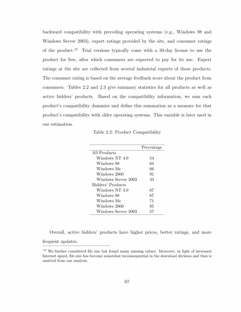
backward compatibility with preceding operating systems (e.g., Windows 98 and
Windows Server 2003), expert ratings provided by the site, and consumer ratings
of the product.12 Trial versions typically come with a 30-day license to use the
product for free, after which consumers are expected to pay for its use. Expert
ratings at the site are collected from several industrial experts of these products.
The consumer rating is based on the average feedback score about the product from
consumers. Tables 2.2 and 2.3 give summary statistics for all products as well as
active bidders’ products. Based on the compatibility information, we sum each
product’s compatibility dummies and define this summation as a measure for that
product’s compatibility with older operating systems. This variable is later used in
our estimation.
Table 2.2: Product Compatibility
PercentageAll Products
Windows NT 4.0 54Windows 98 64Windows Me 66Windows 2000 91Windows Server 2003 43
Bidders’ ProductsWindows NT 4.0 67Windows 98 67Windows Me 71Windows 2000 85Windows Server 2003 57
Overall, active bidders’ products have higher prices, better ratings, and more
frequent updates.
12 We further considered file size but found many missing values. Moreover, in light of increasedInternet speed, file size has become somewhat inconsequential in the download decision and thus isomitted from our analysis.
67

Table 2.3: Product Attributes and Downloads
Mean Std. Dev. Minimum MaximumAll Products
Non-trial Version Price $ 16.65 20.43 0 150Expert Rating (if rated) 3.87 0.81 2 5Average Consumer Rating (if rated) 3.89 1.31 1 5Months Lapse Since Last Update 15.31 9.88 1 31Compatibility Index 3.29 1.47 0 5Number of Downloads/(Product×Month) 1367.29 9257.16 0 184442
Bidders’ ProductsNon-trial Version Price $ 21.97 15.87 0 39.95Expert Rating (if rated) 4 0.50 3 5Average Consumer Rating (if rated) 4.06 0.91 2.5 5Months Lapse Since Last Update 2.38 0.66 1 3Compatibility Index 3.51 1.51 0 5Number of Downloads/(Product×Month) 1992.12 6557.43 0 103454
Consumer File
The consumer file contains the log files of consumers from May 2007 to August 2007.
This file contains each consumer’s browsing log when they visit the search engine
both within the search site and across Internet properties owned by the search site.
The consumer file also has the registration information for those that register.
The browsing log of a consumer records the entry time, browsing path, and
duration of the visit. It also indicates whether the consumer made downloads and,
if yes, which products she downloaded. Upon a user viewing the search results of
software products, the search engine allowed the consumer to sort the results based
on some attributes such as the ratings; consumers can also filter products based on
some criteria such as whether a product’s non-trial version is free. The browsing
log records the sorting and filtering actions of each consumer. Prior to sorting and
filtering, the top five search results are allocated to sponsored search slots and the
remaining slots are ordered by how recently the software has been updated. There
is a small, discrete label indicating whether a search result is sponsored, and sorting
and filtering will often remove these links from the top five premium slots.
As the demographic information upon the registration is only optional, the dataset
provides little if any reliable demographics of consumers. Hence we focus instead
68
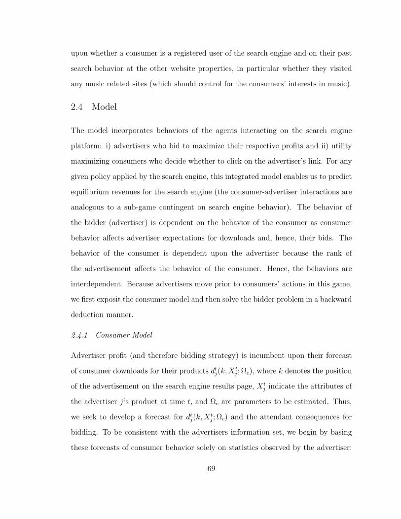
upon whether a consumer is a registered user of the search engine and on their past
search behavior at the other website properties, in particular whether they visited
any music related sites (which should control for the consumers’ interests in music).
2.4 Model
The model incorporates behaviors of the agents interacting on the search engine
platform: i) advertisers who bid to maximize their respective profits and ii) utility
maximizing consumers who decide whether to click on the advertiser’s link. For any
given policy applied by the search engine, this integrated model enables us to predict
equilibrium revenues for the search engine (the consumer-advertiser interactions are
analogous to a sub-game contingent on search engine behavior). The behavior of
the bidder (advertiser) is dependent on the behavior of the consumer as consumer
behavior affects advertiser expectations for downloads and, hence, their bids. The
behavior of the consumer is dependent upon the advertiser because the rank of
the advertisement affects the behavior of the consumer. Hence, the behaviors are
interdependent. Because advertisers move prior to consumers’ actions in this game,
we first exposit the consumer model and then solve the bidder problem in a backward
deduction manner.
2.4.1 Consumer Model
Advertiser profit (and therefore bidding strategy) is incumbent upon their forecast
of consumer downloads for their products dtj(k,Xtj ; Ωc), where k denotes the position
of the advertisement on the search engine results page, X tj indicate the attributes of
the advertiser j’s product at time t, and Ωc are parameters to be estimated. Thus,
we seek to develop a forecast for dtj(k,Xtj ; Ωc) and the attendant consequences for
bidding. To be consistent with the advertisers information set, we begin by basing
these forecasts of consumer behavior solely on statistics observed by the advertiser:
69
the aggregate download data and the distribution of consumers characteristics. Later,
in the policy section of the paper, we assess what happens to bidding behavior and
platform revenues when disaggregate information is revealed to advertisers by the
platform. We begin by describing the consumer’s download decision process and how
it affects the overall number of downloads.
The Consumer Decision Process
Figure 2.2 overviews the decisions made by consumers. In any given period t, the
consumer’s problem is whether and which software to select in order to maximize
their utility. The resolution of this problem is addressed by a series of conditional
decisions.
Figure 2.2: Consumer Decisions
First, the consumer decides whether she should search on the category considered
in this analysis (C1). We presume that the consumer will search on the site if it
maximizes her expected utility.13
Conditioned upon engaging a search, the consumer next decides whether to sort
and/or filter the results (C2). The two search options lead to the following 4 options
for viewing the results: κ =0 ≡ neither, 1 ≡ sorting but not filtering, 2 ≡ not
13 Though we do not explicitly model the consumer’s decision to search across different terms, prod-uct categories or competitors, our model incorporates an ”outside option” that can be interpretedas a composite of these alternative behaviors.
70

sorting but filtering, 3 ≡ sorting and filtering. For each option, the set of products
returned by the search engine differs in terms of the number and the order of products.
Consumers choose the sorting/filtering option that maximizes their expected utility.
Third, the consumer then chooses which, if any products to download (C3). We
presume that consumers choose to download software if it maximizes their expected
utility. We discuss the modeling details for this process in a backward induction
manner (C3–C1).
Download We assume that consumers exhibit heterogeneous preferences for the
products and that these consumers choose products to download to maximize their
expected payoffs. Consumer i of preference segment g (g = 1, 2, ..., G) has some
underlying latent utility ugκijt for downloading software j in period t, conditional on
her sorting/filtering choice κ. A product will be downloaded if and only if ugκijt ≥ 0.
Let a index product attributes
ugκijt = αgj +∑
axκjatβ
ga + εgκijt (2.1)
where
• xκjat is the observed attribute a of product j; product attributes also includes
product j’s slot k on the search page that may vary conditional on sort-
ing/filtering choice κ (hence the superscript κ);
• βga is consumer i’s “taste” regarding product attribute a, which is segment
specific;
• εgκijt’s are individual idiosyncratic preference shocks, realized after the sort-
ing/filtering decision. They are independently and identically distributed over
individuals, products and periods as zero mean normal random variables.
71

To allow the variance of the download (εgκijt) and sorting/filtering errors (ξgκit ,
which will be detailed below) to differ, both must be properly scaled (cf. Train, 2003,
Chapter 2). Hence, we invoke the following assumption:
Assumption 1: εgκijt’s are independently and identically distributed normal random
variables with mean 0 and variance normalized to (δg)2. ξgκit ’s are independently and
identically distributed Type I extreme value random variables.
Under assumption 1, we may re-define the utility in equation 2.1 as
ugκijt = δg(αgj +∑
axκjatβ
ga︸ ︷︷ ︸
ugκijt
+ εgκijt) (2.2)
where αgj , βga , εgκijt = αgj , βga , ε
gκijt/δg; u
gκijt is the scaled “mean” utility and εgκijt ∼
N(0, 1). The resulting choice process is a multivariate probit choice model.14 Let
dijt = 1 stand for downloading and dijt = 0 stand for not downloading. We have
dijt =
10
if ugκijt ≥ 0otherwise
(2.3)
and the probability of downloading conditional on parameters αgj , βga is
Pr(dijt = 1) = Pr(ugκijt ≥ 0) (2.4)
= Pr(δg(ugκijt + εgκijt) ≥ 0)
= Pr(−εgκijt ≤ ugκijt)
= Φ(ugκijt)
where Φ(·) is the standard normal distribution CDF.
Sorting and Filtering Prior to making a download decision, consumers face several
filtering and sorting options which we index as κ = 0, 1, 2, 3. We expect consumers
14 It can be shown that, under very weak assumptions, download decisions across multiple productswith the purpose of maximizing total expected utility can be represented by a multivariate binarychoice probit model.
72

to choose the option that maximizes their expected download utility. Although
consumers know the distribution of the product utility error terms (εgκijt), these error
terms do not realize before the sorting/filtering. Hence consumers can only form an
expectation about the total utilities of all products under a given sorting/filtering
option κ before choosing that option. Let U gκit denote the total expected utility from
products under option κ, which can be calculated based on equation 2.1:
U gκit =
∑j
Eε(ugκijt|u
gκijt ≥ 0) Pr(ugκijt ≥ 0) (2.5)
This definition reflects that a product’s utility is realized only when it is downloaded.
Hence, the expected utility Eε(ugκijt|u
gκijt ≥ 0) is weighted by the download likelihood,
Pr(ugκijt ≥ 0). The expectation, Eε(·), is taken over the random preference shocks εgκijt.
In addition to U gκit , individuals may accrue additional benefits or costs for using
sorting/filtering option κ. These benefits or costs may arise from individual differ-
ences of efficiency or experience in terms of engaging the various options for ordering
products. We denote such benefits or costs by random terms ξgκit ’s. As indicated in
assumption 1, ξgκit ’s are i.i.d. Type I extreme value. ξgκit is not observed by researchers
but known to individual i. Note that these sorting/filtering benefits or costs do not
materialize during the consumption of the products. Therefore, they do not enter
the latent utility in equation (2.1). The total utility of search option κ is thus given
by
zgκit = U gκit + ξgκit (2.6)
Consumers choose the option of sorting/filtering that leads to the highest total utility
zgκit .
With ξgκit following a Type I extreme value distribution, the choice of sort-
73
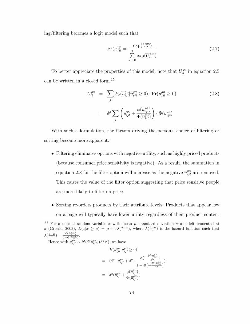
ing/filtering becomes a logit model such that
Pr(κ)git =exp(U gκ
it )3∑
κ′=0
exp(U gκ′
it )
(2.7)
To better appreciate the properties of this model, note that U gκit in equation 2.5
can be written in a closed form.15
U gκit =
∑j
Eε(ugκijt|u
gκijt ≥ 0) · Pr(ugκijt ≥ 0) (2.8)
= δg∑j
(ugκijt +
φ(ugκijt)
Φ(ugκijt)
)· Φ(ugκijt)
With such a formulation, the factors driving the person’s choice of filtering or
sorting become more apparent:
• Filtering eliminates options with negative utility, such as highly priced products
(because consumer price sensitivity is negative). As a result, the summation in
equation 2.8 for the filter option will increase as the negative ugκijt are removed.
This raises the value of the filter option suggesting that price sensitive people
are more likely to filter on price.
• Sorting re-orders products by their attribute levels. Products that appear low
on a page will typically have lower utility regardless of their product content
15 For a normal random variable x with mean µ, standard deviation σ and left truncated ata (Greene, 2003), E(x|x ≥ a) = µ + σλ(a−µ
σ ), where λ(a−µσ ) is the hazard function such that
λ(a−µσ ) = φ( a−µ
σ )
1−Φ( a−µσ )
.
Hence with ugκijt ∼ N(δgugκ
ijt, (δg)2), we have
E(ugκijt|u
gκijt ≥ 0)
= (δg · ugκijt + δg ·
φ(− δg·ugκijt
δg )
1− Φ(− δg·ugκijt
δg ))
= δg(ugκij +
φ(ugκij )
Φ(ugκij )
)
74

(because consumer slot rank sensitivity is negative). For example, suppose
a consumer relies more on product ratings. By moving more desirable items
that have high ratings up the list, sorting can increase the ugκijt for these items,
thereby increasing the resulting summation in equation 2.8 and the value of
this sorting option. 16
Keyword Search The conditional probability of keyword search takes the form
Pr(searchgi ) =exp(λg0 + λg1IV
git )
1 + exp(λg0 + λg1IVgit )
(2.9)
where IV gi is the inclusive value for searching conditional on the segment member-
ship. IV git is defined as
IV git = log[
∑κexp(U gκ
it )] (2.10)
This specification can be interpreted as the consumer making a decision to use a
keyword search based on the rational behavior of utility maximization (McFadden,
1977; Ben-Akiva and Lerman, 1985).17 A search term is more likely to be invoked if
it yields higher expected utility.
Segment Membership Recognizing that consumers are heterogeneous in behaviors
described above, we apply a latent class model in the spirit of Kamakura and Russell
(1989) to capture heterogeneity in consumer preferences. Heterogeneity in preference
can arise, for example, when some consumers prefer some features more than others.
We assumeG exogenously determined segments.18 Note that our specification implies
16 In particular, in the data over 80% of consumers who used sorting option chose ratings to re-order products. Thus, we suspect that consumers who rely on ratings are more likely to use thesorting option to see which items are the most popular ones.17 This specification is consistent with the consumer information structure such that ξgκ
i is notobserved by researchers but known to consumer i.18 It is possible to allow for continuous mixtures of heterogeneity as well. In our application, manyconsumers enter only once, making it difficult to identify a consumer specific term for them.
75

a dependency across decisions within the same segment that is not captured via
the stage-specific decision errors, and therefore captures the effect of unobserved
individual specific differences in search behavior.
The prior probability for user i being a member of segment g is defined as
pggit = exp (γg0 +Demo′itγg) /ΣG
g′=1 exp(γg
′
0 +Demo′itγg′)
(2.11)
where Demo′it is a vector of attributes of user i such as demographics and past
browsing history; vector γg0 , γg∀g contains parameters to be estimated. For the
purpose of identification, one segment’s parameters are normalized to zero.
Consumer Downloads
The search, sort/filter and download models can be integrated to obtain an expec-
tation of the number of downloads that an advertiser receives for a given position
of its keyword advertisement. Advertisers must form this expectation predicated on
observed aggregate download totals, dtj (in contrast to the search engine who observes
yijt, κit and Demoit).19
To develop this aggregate download expectation, we begin by noting that the
download utility ugκijt is a function of consumer specific characteristics and decisions
ζijt = [εgκijt, ξgκit , search
gi , segment g membership, Demo′it] and that an advertiser needs
to develop an expectation of downloads over the distribution of these unobserved (to
the advertiser) individual characteristics. Define
Aijt = ζijt : ugκijt ≥ 0
i.e., Aijt is the set of values of ζijt which will lead to the download of product j in
period t.
19 We discuss the corresponding advertiser download expectation under complete information insection 2.7.3.
76

Let D(ζijt) denote the distribution of ζijt. The likelihood of downloading product
j in period t can be expressed as
P tj =
∫ζijt∈Aijt
D(ζijt) (2.12)
=
∫Demoit
∑g
∑κ[Φ(ugκijt)
exp(U gκit )
3∑κ′=0
exp(U gκ′
it )
] Pr(searchgit)pggitdD(Demoit)
where the first term in the brackets captures the download likelihood, the second
term captures the search strategy likelihood, and the first term outside the brackets
captures the likelihood of search. pggit is the probability of segment g membership
and D(Demoit) is the distribution of demographics.
Correspondingly, the advertiser with attributes X tj has an expected number of
downloads for appearing in slot k, dtj(k,Xtj ; Ωc), which can be computed as follows
dtj(k,Xtj ; Ωc) = MtP
tj (2.13)
where Ωc is the set of consumer preference parameters; Mt is the market size in
period t; and X tj is the vector of the a product characteristics, xjat.
Product attributes are posted on the search engine and are therefore common
knowledge to all advertisers and consumers. We assume these X tj are exogenous
within the scope of our sponsored search analysis for several reasons. First, adver-
tisers distribute and promote their products through multiple channels and they do
so over longer periods of time than considered herein. Hence, product attributes are
more likely to be determined via broader strategic considerations than the particu-
lar auction game and time frame we consider. Second, the attribute levels for each
product are stable over the duration of our data and analysis. We would expect more
variation in attribute levels if they were endogenous to the particular advertiser and
77

search engine decisions we consider. Third, because there is little or no variation
in product attributes over time, it is not feasible to estimate endogenous attribute
decision making with our data.
2.4.2 Advertiser Model
Figure 2.3 overviews the dynamic game played by the advertiser. Advertiser j’s
problem is to decide the optimal bid amount btj with the objective of maximizing
discounted present value of payoffs.20 Higher bids lead to greater revenues because
they yield more favorable positions on the search engine, thereby yielding more click-
throughs for the advertiser. However, higher bids also increase costs (payments)
leading to a trade-off between costs and revenues. The optimal decision of whether
and how much to bid is incumbent upon the bidding mechanism, the characteristics
of the advertiser, the information available at the time of bidding (including the state
variables), and the nature of competitive interactions.
An advertiser’s period profit for a download is the value it receives from the
download less the costs (payments) of the download. Though we do not observe the
value of a download, we infer this value by noting the observed bid can be rationalized
only for a particular value accrued by the advertiser. We presume this value is drawn
from a distribution known to all firms. The total period revenue for the advertiser is
then the value per download times the expected number of downloads.21 The total
period payment upon winning is the number of downloads times the advertiser’s bid.
Hence, the total expected period profit is the number of downloads times the profit
per download (i.e., the value per downloads less the payment per download).
20 Because the search engine used in our application has the dominant market share in the con-sidered category, we do not address advertiser bidding on other sites. Also, it would be difficult toobtain download data from these more minor competitors. We note this is an important issue andcall for future research.21 The expected number of downloads is inferred form the consumer model and we have derivedthis expression in section 2.4.1.
78
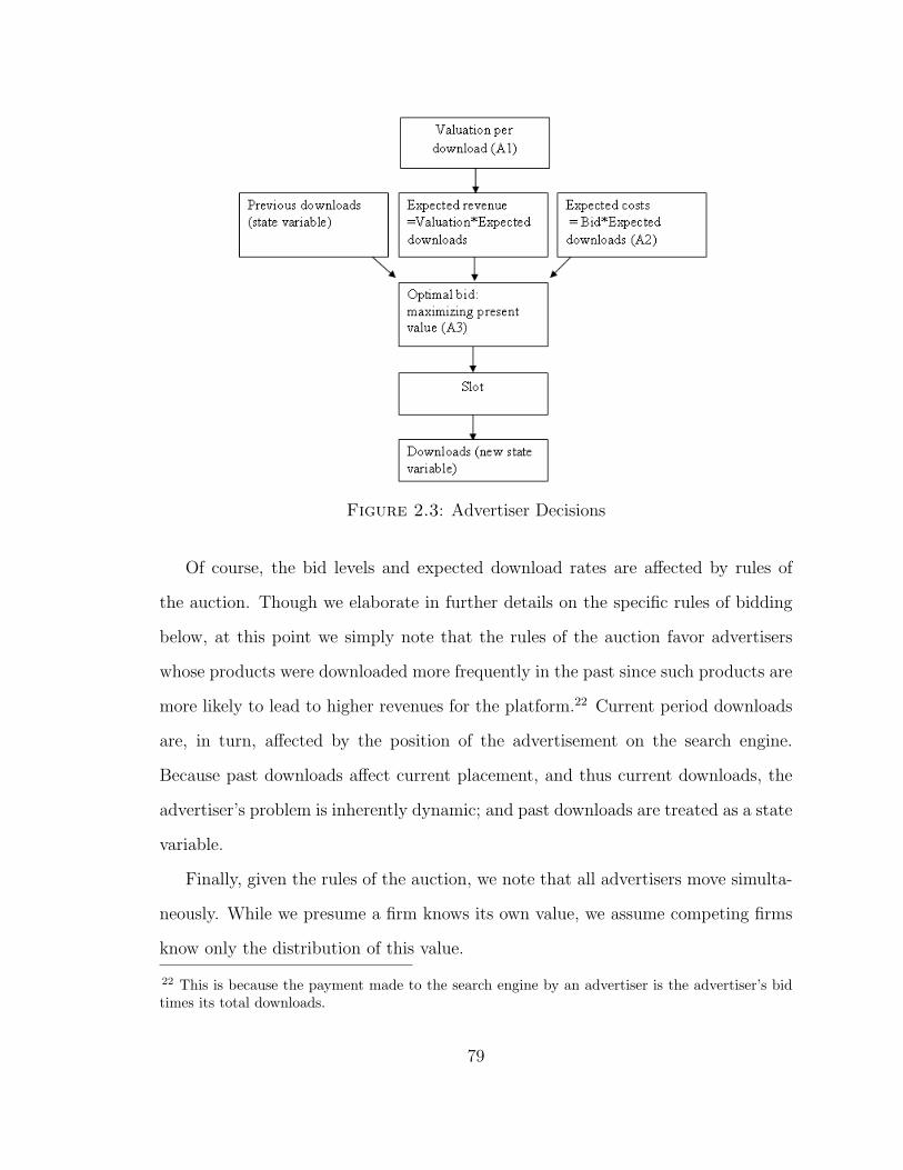
Figure 2.3: Advertiser Decisions
Of course, the bid levels and expected download rates are affected by rules of
the auction. Though we elaborate in further details on the specific rules of bidding
below, at this point we simply note that the rules of the auction favor advertisers
whose products were downloaded more frequently in the past since such products are
more likely to lead to higher revenues for the platform.22 Current period downloads
are, in turn, affected by the position of the advertisement on the search engine.
Because past downloads affect current placement, and thus current downloads, the
advertiser’s problem is inherently dynamic; and past downloads are treated as a state
variable.
Finally, given the rules of the auction, we note that all advertisers move simulta-
neously. While we presume a firm knows its own value, we assume competing firms
know only the distribution of this value.
22 This is because the payment made to the search engine by an advertiser is the advertiser’s bidtimes its total downloads.
79

The process is depicted in Figure 2.3. We describe the process with more details
as follows: Section 2.4.2 details the rules of the auction that affect the seller costs
(A2), section 2.4.2 details the advertisers’ value distribution (A1), and section 2.4.2
indicates how period values and costs translate to discounted profits and the resulting
optimal bidding strategy (A3).
Seller Costs and the Bidding Mechanism
We begin by discussing how slot positions are allocated with respect to bids and the
effect of these slot positions on consumer downloads (and thus advertiser revenue).
Upon a consumer completing a query, the search engine returns k = 1, 2, ...K, ..., N
slots covering the products of all firms. Only the top K = 5 slots are consid-
ered as premium slots. Auctions for these K premium slots are held every period
(t = 1, 2, ...). An advertiser seeks to appear in a more prominent slot because this
may increase demand for the advertiser’s product. Slots K+1 to N are non-premium
slots which compose a section called organic search section.
There are N advertisers who are interested in the premium slots (N ≤ N).
In order to procure a more favorable placement, advertiser j submits bid btj in
period t. These bids, submitted simultaneously, are summarized by the vector
bt = bt1, bt2, ..., btN.23 Should an advertiser win slot k, the realized number of down-
loads dtj is a random draw from the distribution with the expectation dtj(k,Xtj ; Ωc).
The placement of advertisers into the K premium slots is determined by the ranking
of their btjdt−1j ∀j, i.e., the product of current bid and last period realized downloads;
the topmost bidder gets the best premium slot; the second bidder gets the second
best premium slot; and so on. A winner of one premium slot pays its own bid btj
for each download in the current period. Hence, the total payment for winning the
23 For the purpose of a clear exposition, we sometimes use boldface notations or pairs of bracesto indicate vectors whose elements are variables across all bidders. For example, dt = dt
j∀j is avector whose elements are dt
j ,∀j.
80

auction is btjdtj.
If an advertiser is not placed at one of the K premium slots, it will appear in the
organic section; advertisers placed in the organic section do not pay for downloads
from consumers. The ranking in the organic search section is determined by the
product update recency at period t, which is a component of the attribute vector of
each product, X tj . Other attributes include price, consumer ratings, and so on.
Given that the winners are determined in part by the previous period’s downloads,
the auction game is inherently dynamic. Before submitting a bid, the commonly
observed state variables at time t are the realized past downloads of all bidders from
period t− 1,24
st = dt−1 = dt−11 , dt−1
2 , ..., dt−1N (2.14)
Seller Value
The advertiser’s bid determines the cost of advertising and must be weighed against
the potential return when deciding how much to bid. We denote advertiser j’s
valuation regarding one download of its product in period t as vtj. We assume that
this valuation is private information but drawn from a normal distribution that is
commonly known to all advertisers. Specifically,
vtj = v(X tj ; θ) + fj + rtj (2.15)
= X tjθ + fj + rtj
where θ are parameters to be estimated and reflect the effect of product attributes on
valuation. The fj are firm-specific fixed effect terms assumed to be identically and
independently distributed across advertisers. This fixed effect term captures hetero-
geneity in valuations that may arise from omitted firm-specific effects such as more
24 Though state variables can be categorized as endogenous (past downloads) and exogenous (prod-uct attributes), our exposition characterizes only downloads as state variables because these are theonly states whose evolution is subject to a dynamic constraint.
81

efficient operations. The rtj ∼ N(0, ψ2) are private shocks to an advertiser’s valuation
in period t, assumed to be identically and independently distributed across adver-
tisers and periods. The sources of this private shock may include: (1) temporary
increases in the advertiser’s valuation due to some events such as a promotion cam-
paign; (2) unexpected shocks to the advertiser’s budget for financing the payments of
the auction; (3) temporary production capacity constraint for delivering the product
to users; and so on. The random shock rtj is realized at the beginning of period t.
Although rtj is private knowledge, we assume the distribution of rtj ∼ N(0, ψ2) is
common knowledge among bidders. We further assume the fixed effect fj of bid-
der j is known to all bidders but not to researchers. Given bidders may observe
opponents’ actions for many periods, the fixed effect can be inferred among bidders
(Greene, 2003).
Seller Profits: A Markov Perfect Equilibrium (MPE)
Given vtj and state variable st, predicted downloads and search engine’s auction
rules, bidder j decides the optimal bid amount btj with the objective of maximizing
discounted present value of payoffs. In light of this, every advertiser has an expected
period payoff, which is a function of st, Xt, rtj and all advertisers’ bids bt
Eπj(bt, st,Xt, rtj; θ, fj
)(2.16)
= E∑K
k=1Pr(k|btj,bt−j, st,Xt
)· (vtj − btj) · dtj(k,X t
j ; Ωc)
+E∑N
k=K+1Pr(k|btj,bt−j, st,Xt
)· vtj · dtj(k,X t
j ; Ωc)
= E∑K
k=1Pr(k|btj,bt−j, st,Xt
)· (X t
jθ + fj + rtj − btj) · dtj(k,X tj ; Ωc)
+E∑N
k=K+1Pr(k|btj,bt−j, st,Xt
)· (X t
jθ + fj + rtj) · dtj(k,X tj ; Ωc)
82

where the expectation for profits is taken over other advertisers’ bids bt−j. Pr (k|·)
is the conditional probability of advertiser j getting slot k, k = 1, 2, ..., N . Pr (k|·)
depends not only on bids, but also on states st (the previous period’s downloads)
and product attributes Xt.25 This is because: i) the premium slot allocation is
determined by the ranking of btjdt−1j ∀j, where dt−1 are the state variables and ii)
the organic slot allocation is determined by product update recency, an element of
Xt.
In addition to the current period profit, an advertiser also takes its expected
future payoffs into account when making decisions. In period t, given the state
vector st, advertiser j’s discounted expected future payoffs evaluated prior to the
realization of the private shock rtj is given by
E[∑∞
τ=tρτ−tπj
(bτ , sτ ,Xτ , rτj ; Ωaj
)|st]
(2.17)
where Ωaj = θ, ψ, fj, with a denoting advertiser behavior (in contrast to the pa-
rameters Ωc in the consumer model). Further, we denote Ωa = Ωajj=1,2,...,N =
θ, ψ, fjj=1,2,...,N . The parameter ρ is a common discount factor. The expectation
is taken over the random term rtj, bids in period t as well as all future realization
of Xt, shocks, bids, and state variables. The state variables st+1 in period t + 1 is
drawn from a probability distribution P (st+1|bt, st,Xt).
We use the concept of a pure strategy Markov perfect equilibrium (MPE) to
model the bidder’s problem of whether and how much to bid in order to maximize
the discounted expected future profits (Bajari et al., 2007; Ryan and Tucker, 2008;
Dube et al., 2008; and others). The MPE implies that each bidder’s bidding strategy
only depends on the then-current profit-related information, including state, Xtand
its private shock rtj. Hence, we can describe the equilibrium bidding strategy of bidder
25 Note that st and Xt are observed by all bidders before bidding.
83

j as a function σj(st,Xt, rtj
)= btj.
26 Given a state vector s, product attributes X
and prior to the realization of current rj (with the time index t suppressed), bidder
j’s expected payoff under the equilibrium strategy profile σ = σ1, σ2, ..., σN can be
expressed recursively as:
Vj (s,X;σ) = E
[πj (σ, s,X, rj; Ωa) + ρ
∫s′Vj (s′,X′;σ) dP (s′|b, s,X) |s
](2.18)
where the expectation is taken over current and future realizations of random terms
r and X. To test the alternative theory that advertiser’s may be myopic in their
bidding, we will also solve the advertiser problem under the assumption that period
profits are maximized independently over time.
The advertiser model can then be used in conjunction with the consumer model
to forecast advertiser behavior as we shall discuss in the policy simulation section.
In a nutshell, we presume advertisers will choose bids to maximize their expected
profits. A change in information states, bidding mechanisms, or webpage design will
lead to an attendant change in bids conditioned on the advertisers value function,
which we estimate as described next.
2.5 Estimation
2.5.1 An Overview
Though it is standard to estimate dynamic MPE models via a dynamic programming
approach such as a nested fixed point estimator (Rust, 1994), this requires one to
repetitively evaluate the value function (equation 2.18) through dynamic program-
ming for each instance in which the parameters of the value function are updated.
Even when feasible, it is computationally demanding to implement this approach.
26 The bidding strategies are individual specific due to the fixed effect fj (hence the subscript j).For the purpose of clear exposition, we use σj
(st,Xt, rt
j
)instead of σj
(st,Xt, rt
j ; fj
)throughout
the paper. Multiple observations for each advertiser allows the identification of σj , j = 1, 2, ...N .
84

Instead, we consider the class of two-step estimators. The two-step estimators are
predicated upon the notion that the dynamic program can be estimated in two steps
that dramatically simplify the estimation process by facilitating the computation
of the value function. Specifically, in this application we implement the two-step
estimator proposed by Bajari et al. (2007) (BBL henceforth).
As can be seen in equation 2.18, the value function is parameterized by the
primitives of the value distribution Ωa. Under the assumption that advertisers are
behaving rationally, these advertiser private values for clicks should be consistent
with observed bidding strategies. Therefore, in the second step estimation, values of
Ωa are chosen so as to make the observed bidding strategies congruent with rational
behavior. We detail this step in Section 2.5.3 below.
However, as can be observed in equations 2.18 and 2.16, computation of the value
function is also incumbent upon i) the bidding policy function that maps bids to the
states (downloads), product attributes, and private shocks σj(st,Xt, rtj
)= btj; ii) the
expected downloads dtj(k,Xtj ; Ωc); and iii) a function that maps the likelihood of
future states as a function of current states and actions P (st+1|bt, st,Xt). These are
estimated in the first step as detailed in Section 2.5.2 below and then substituted
into the value function used in the second step estimation.
2.5.2 First Step Estimation
In the first step of the estimation we seek to obtain:
1. A “partial” policy function σj (s,X) describing the equilibrium bidding strate-
gies as a function of the observed state variables and product attributes, X. We
estimate the policy function by noting that players adopt equilibrium strategies
(or decision rules) and that behaviors generated from these decision rules lead
to correlations between i) the observed states (i.e., past period downloads) and
product characteristics and ii) advertiser decisions (i.e., bids). The partial pol-
85
icy function captures this correlation. In our case, we use a fixed effects Tobit
model to link bids to states and product characteristics as described in Section
4.2.1 of the Appendix. Subsequently, the full policy function σj(s,X, rtj
)can
be inferred based on σj (s,X) and the distribution of private random shocks rtj.
The partial policy function can be thought of as the marginal distribution of
the full policy function. Inferences regarding the parameters of the full policy
function can be made by finding the distribution of rtj that, when “integrated
out,” leads to the best rationalization for the observed bids. We discuss our
approach to infer the full policy functions from the partial policy function in
Appendix 4.2.1.
2. The expected downloads for a given firm at a given slot, dtj(k,Xj; Ωc). The
dtj(k,Xj; Ωc) follows directly from the consumer model. Hence, the first step
estimation involves i) estimating the parameters of the consumer model and
then ii) using these estimates to compute the expected number of downloads.
The expected total number of downloads as a function of slot position and
product attributes is obtained by using the results of the consumer model
to forecast the likelihood of each person downloading the software and then
integrating these probabilities across persons.27 We discuss our approach for
determining the expected downloads in Section 4.2.1 of the Appendix.
3. The state transition probability P (s′|b, s,X) which describes the distribution
of future states (current period downloads) given observations of the current
state (past downloads), product attributes, and actions (current period bids).
27 As an aside, we note that advertisers have limited information from which to form expecta-tions about total downloads because they observe the aggregate information of downloads but notthe individual specific download decisions. Hence, advertisers must infer the distribution of con-sumer preferences from these aggregate statistics. In a subsequent policy simulation we allow thesearch engine to provide individual level information to advertisers in order to assess how it affectsadvertiser behavior and, therefore, search engine revenues.
86
These state transitions can be derived by i) using the policy function to predict
bids as a function of past downloads, ii) determining the slot ranking as a
function of these bids, past downloads and product attributes, and then iii)
using the consumer model to predict the number of current downloads as a
function of slot position. Details regarding our approach to determining the
state transition probabilities is outlined in Section 4.2.1 of the Appendix.
With the first step estimates of σj(s,X, rtj
), dtj(k,Xj; Ωc), and P (s′|b, s,X), we
can compute the value function in equation 2.18 as a function with only Ωa unknown.
In the second step, we estimate these parameters.
2.5.3 Second Step Estimation
The goal of the second step estimation is to recover the primitives of the bidder
value function, Ωa. The intuition behind how the second-stage estimation works is
that true parameters should rationalize the observed data. For bidders’ data to be
generated by rational plays, we need
Vj (s,X;σj, σ−j; Ωa) ≥ Vj(s,X;σ′j, σ−j; Ωa
),∀σ′j 6= σj (2.19)
where σj is the equilibrium policy function and σ′j is some deviations from σj. This
equation means that any deviations from the observed equilibrium bidding strategy
will not result in more profits. Otherwise, the strategy would not be optimal. Hence,
we first simulate the value functions under the equilibrium policy σj and the deviated
policy σ′j (i.e., the left hand side and the right hand side of equation 2.19). Then
we choose Ωa to maximize the likelihood that equation 2.19 holds. We describe the
details of this second step estimation in Appendix 4.2.1.
2.5.4 Sampling Chain
With the posterior distributions for the advertiser and consumer models established,
we estimate the models using MCMC approach as detailed in Appendix 4.2.2. This
87

is a notable deviation from prior research that uses a gradient based technique. The
advantage of using a Bayesian approach, as long as suitable parametric assumptions
can be invoked, is that it facilitates model convergence, has desirable small sam-
ple properties, increases statistical efficiency, and enables the estimation of a wide
array of functional forms (Rossi et al., 2005). Indeed, posterior sampling distri-
butions for many of the parameters are highly skewed and/or have thin tails, and
Kolmogorov-Smirnov tests indicate these posterior distributions are often not nor-
mally distributed. Hence, we seek to make a methodological contribution to the
burgeoning literature on two-step estimators for dynamic games.
2.6 Results
2.6.1 First Step Estimation Results
Recall, the goal of the first step estimation is to determine the policy function,
σj(st,Xt, rtj
), the expected downloads dtj(k,X
tj ; Ωc), and the state transition prob-
abilities P (st+1|bt, st,Xt) . To determine σj(st,Xt, rtj
), we first estimate the partial
policy function σj (st,Xt) and then compute the full policy function. To determine
dtj(k,Xtj ; Ωc), we first estimate the consumer model and then compute the expected
downloads. Last P (st+1|bt, st,Xt) is derived from the consumer model and the par-
tial policy function. Thus, in the first stage we need only to estimate the partial
policy function and the consumer model. With these estimates in hand, we compute
σj(st,Xt, rtj
), dtj(k,X
tj ; Ωc), and P (st+1|bt, st,Xt) for use in the second step. Thus,
below, we report the estimates for the partial policy function and the consumer
model on which these functions are all based.
Partial Policy Function σj(s,X)
The vector of independent variables (s,X) for the partial policy function (i.e., the
Tobit model of advertiser behavior that captures their bidding policy as outlined in
88
Appendix section 4.2.1) contains the following variables:
• Product j’s state variable, last period download dt−1j . We reason that high
past downloads increase the likelihood of a favorable placement and, therefore,
affect bids.
• Two market level variables: the sum of last period downloads from all bidders
and the number of bidders in last period. Since we only have 322 observa-
tions of bids, it is infeasible to estimate a parameter to reflect the effect of
each opponent’s state (i.e., competition) on the optimal bid. Moreover, it is
unlikely a bidder can monitor every opponent’s state in each period before
bidding because such a strategy carries high cognitive and time costs. Hence,
summary measures provide a reasonable approximation of competing states in
a limited information context. Others in the literature who have invoked a
similar approach include Jofre-Bonet and Pesendorfer (2003) and Ryan (2006).
Like them, we find this provides a fair model fit. Another measure of compet-
itive intensity is the number of opponents. Given that bidders cannot directly
observe the number of competitors in the current period, we used a lagged
measure of the number of bidders.
• Product j’s attributes in period t (X tj), including its non-trial version price,
expert rating, consumer rating, update recency, and compatibility with an
older operating system. We expect that a higher quality product will yield
greater downloads thereby affecting the bidding strategy.
• An advertiser specific constant term to capture the impact of the fixed effect
fj on bidding strategy.
• To control the possible effect of the growth of ownership of MP3 players, we
also collect the average lagged price of all new MP3 players in the market from
89
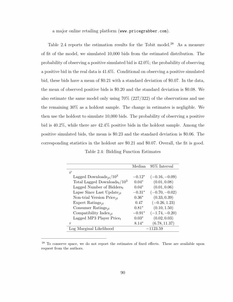
a major online retailing platform (www.pricegrabber.com).
Table 2.4 reports the estimation results for the Tobit model.28 As a measure
of fit of the model, we simulated 10,000 bids from the estimated distribution. The
probability of observing a positive simulated bid is 42.0%; the probability of observing
a positive bid in the real data is 41.6%. Conditional on observing a positive simulated
bid, these bids have a mean of $0.21 with a standard deviation of $0.07. In the data,
the mean of observed positive bids is $0.20 and the standard deviation is $0.08. We
also estimate the same model only using 70% (227/322) of the observations and use
the remaining 30% as a holdout sample. The change in estimates is negligible. We
then use the holdout to simulate 10,000 bids. The probability of observing a positive
bid is 40.2%, while there are 42.4% positive bids in the holdout sample. Among the
positive simulated bids, the mean is $0.23 and the standard deviation is $0.06. The
corresponding statistics in the holdout are $0.21 and $0.07. Overall, the fit is good.
Table 2.4: Bidding Function Estimates
Median 95% Intervalϕ
Lagged Downloadsjt/103 −0.12∗ (−0.16,−0.09)Total Lagged Downloadst/103 0.04∗ (0.01, 0.08)Lagged Number of Bidderst 0.04∗ (0.01, 0.06)Lapse Since Last Updatejt −0.31∗ (−0.70,−0.02)Non-trial Version Pricejt 0.36∗ (0.33, 0.39)Expert Ratingsjt 0.47 (−0.26, 1.23)Consumer Ratingsjt 0.81∗ (0.10, 1.50)Compatibility Indexjt −0.91∗ (−1.74,−0.20)Lagged MP3 Player Pricet 0.03∗ (0.02, 0.03)
τ 8.14∗ (6.78, 11.37)Log Marginal Likelihood −1123.59
28 To conserve space, we do not report the estimates of fixed effects. These are available uponrequest from the authors.
90

The estimates yield several insights into the observed bidding strategy. First, the
bidder’s state variable (dt−1j ) is negatively correlated with its bid amount btj because
the ranking of the auction is determined by the product of btj and dt−1j . All else
being equal, a higher number of lagged downloads means a bidder can bid less to
obtain the same slot. Second, the total number of lagged downloads in the previous
period (∑
j′ dt−1j′ ) and the lagged number of bidders both have a positive impact on
a bidder’s bid. We take this to mean increased competition leads to higher bids.
Third, bids are increasing in the product price. One possible explanation is that a
high priced product yields more value to the firm for each download, and hence the
firm competes more aggressively for a top slot. Similarly and fourth, a high price
for MP3 players reflects greater value for the downloads also leading to a positive
effect on bids. Fifth, “Lapse Since Last Update” has a negative effect on bids. Older
products are more likely obsolete, thereby generating lower value for consumers. If
this is the case, firms can reasonably expect fewer final purchases after downloads
and, therefore, bid less for these products. Likewise and sixth, higher compatibility
with prior software versions reflects product age leading to a negative estimate for
this variable. Finally, ratings from consumers and experts (albeit not significant for
experts) have a positive correlation with bid amounts – these again imply greater
consumer value for the goods, making it more profitable to advertise them.
Consumer Model
The consumer model is estimated using MCMC approach based on the posterior
distribution described in Appendix 4.2.1. We consider the download decisions for
each of the 21 products who entered auctions, plus the top 3 products who did not.
Together these firms constitute over 80% of all downloads. The remaining number of
downloads are scattered across 370 other firms, each of whom has a negligible share.
Hence, we exclude them from our analysis.
91

Table 2.5: Alternative Numbers of Latent Segments
Log Marginal Likelihood1 Segment −12769.32 Segments∗ −12511.93 Segments −12571.14 Segments −12551.4
We calibrate the model by estimating an increasing number of latent segments
until there is no significant improvement in model fit. We use log marginal likelihood
as the measurement for model fit. In Table 2.5 we report the comparison of the log
marginal likelihoods for models with up to four segments. The model with two
segments gives the best result in terms of maximizing the log marginal likelihood.
Table 2.6 presents the estimates of the model with two segments. Conditional on
the estimated segment parameters and demographic distribution, we calculate the
segment sizes as 89.5% and 10.5%, respectively. Based on the parameter estimates
in Table 2.6, Segment 1 is less likely to initiate a search (low λg0). The primary
basis of segmentation is whether a customer has visited a music website at other
properties owned by the download website; these customers are far more likely to be
in the frequent download segment. Moreover, upon engaging a search, this segment
appears to be less sensitive to slot ranking but more sensitive to consumer and expert
ratings than segment 2. Segment 2, composed of those who searche more frequently,
relies more heavily on the slot order when downloading. Overall, we speculate that
searchers in segment 1 are the occasional downloaders who base their download
decisions on others’ ratings and tend not to exclude goods of high price. In contrast,
segment 2 contains the “experts” or frequent downloaders who tend to rely on their
own assessments when downloading. Of interest is the finding that those in segment
2 rely more on advertising slot rank. This is consistent with a perspective that
frequent downloaders might be more strategic; knowing that higher quality firms
92

Table 2.6: Consumer Model Estimates
Segment 1 (89.5%)(Infrequent searcher)
Segment 2 (10.5%)(Frequent searcher and slot sensitive)
Median(95%Interval)
Median(95%Interval)
βg (utility parameters)Constant −0.09
(−0.11,0.001)0.35
(0.31,0.38)
Slot Rank −0.08(−0.06,−0.09)
−0.51(−0.52,−0.50)
Non-trial Version Price 0.03(0.03,0.04)
−0.04(−0.04,−0.03)
Expert Ratings 0.16(0.15,0.17)
0.06(0.06,0.07)
Consumer Ratings 0.11(0.11,0.12)
0.03(0.03,0.05)
Compatibility Index −0.08(−0.09,−0.07)
0.16(0.16,0.17)
Total Download Percentage 0.01(−0.02,0.05)
0.09(0.08,0.10)
δg (sorting/filtering scaling) 1.52(1.48,1.55)
1.87(1.78,1.99)
λg (search probability)λg0 (base) −10.22
(−10.75,−9.60)−0.78
(−1.21,−0.54)
λg1 (1-correlation) 0.02(0.01,0.02)
0.03(0.01,0.04)
γg (segment parameters)Constant − −4.01
(−4.74,−2.87)
Music Site Visited − 7.66(5.77,10.18)
Registration Status − −0.24(−1.91,0.86)
Product Downloadedin Last Month
− −0.40(−1.57,−0.02)
tend to bid more and obtain higher ranks, those who download often place greater
emphasis on this characteristic.
More insights on this difference in download behavior across segments can be
gleaned by determining the predicted probabilities of searching and sorting/filtering
by computing Pr(searchgi ) =exp(λg0+λg1IV
git)
1+exp(λg0+λg1IVgit)
and Pr(κ)git =exp(Ugκit )
3Pκ′=0
exp(Ugκ′
it )
in equations
2.9 and 2.7, respectively. Table 2.7 reports these probabilities for both segments.
Table 2.7 confirms the tendency of segment 2 to be more likely to initiate a
93
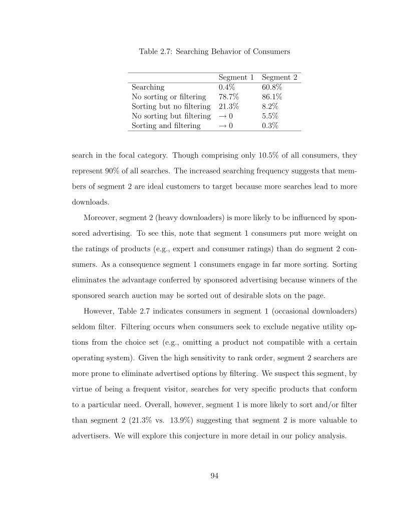
Table 2.7: Searching Behavior of Consumers
Segment 1 Segment 2Searching 0.4% 60.8%No sorting or filtering 78.7% 86.1%Sorting but no filtering 21.3% 8.2%No sorting but filtering → 0 5.5%Sorting and filtering → 0 0.3%
search in the focal category. Though comprising only 10.5% of all consumers, they
represent 90% of all searches. The increased searching frequency suggests that mem-
bers of segment 2 are ideal customers to target because more searches lead to more
downloads.
Moreover, segment 2 (heavy downloaders) is more likely to be influenced by spon-
sored advertising. To see this, note that segment 1 consumers put more weight on
the ratings of products (e.g., expert and consumer ratings) than do segment 2 con-
sumers. As a consequence segment 1 consumers engage in far more sorting. Sorting
eliminates the advantage conferred by sponsored advertising because winners of the
sponsored search auction may be sorted out of desirable slots on the page.
However, Table 2.7 indicates consumers in segment 1 (occasional downloaders)
seldom filter. Filtering occurs when consumers seek to exclude negative utility op-
tions from the choice set (e.g., omitting a product not compatible with a certain
operating system). Given the high sensitivity to rank order, segment 2 searchers are
more prone to eliminate advertised options by filtering. We suspect this segment, by
virtue of being a frequent visitor, searches for very specific products that conform
to a particular need. Overall, however, segment 1 is more likely to sort and/or filter
than segment 2 (21.3% vs. 13.9%) suggesting that segment 2 is more valuable to
advertisers. We will explore this conjecture in more detail in our policy analysis.
94

2.6.2 Second Step Estimation Results
Alternative Models
In addition to our proposed model, we consider two alternative models of seller behav-
ior: i) myopic bidding and ii) heterogeneous valuations across consumer segments.29
Table 2.8 reports the fit of each model. In the first alternative model, advertisers
maximize period profits independently as opposed to solving the dynamic bidding
problem given in equation 2.18. This model yields a considerably poorer fit. Hence,
we conclude that advertisers are bidding strategically. This strategic behavior might
result from dynamics in the bidding process coupled with non-linearities in advertis-
ing response. Similar dynamic behavior has been evidenced in the face of non-linear
advertising demand systems with dynamics in advertising carryover (Bronnenberg,
1998).
The second model considers the case wherein advertiser valuations for clicks differ
across segments. In this model, we augment equation 2.15 by allowing it to vary by
segment and then integrate this heterogeneity into the seller profit function given by
equation 2.16. This model leads to only a negligible increase in fit. Closer inspection
of the results indicates little difference in valuations across segments, implying ad-
vertisers perceive that the conversion rates of each segment are essentially the same.
Hence, we adopt the more parsimonious single valuation model. It is further worth
noting that all of our subsequent results and policy simulations evidence essentially
no change across these two models.
29 We do not estimate the discount factor ρ. As shown in Rust (1994), the discount factor is usuallyunidentified. We fix ρ = 0.95 for our estimation. We also experiment at ρ = 0.90 and see minimaldifference in the results.
95

Table 2.8: Alternative Models
Model Log Marginal LikelihoodBase Model −1651.3Base Model Without Advertiser Dynamics −1701.3Base Model With Heterogeneous Customer Valuations −1645.1
Valuation Model Results
Table 2.9 shows the results of second step estimation for the favored model.30 With
respect to the advertiser value function, we find that newer, more expensive and
better rated products yield greater values to the advertiser. This is consistent with
our conjecture in Section 2.6.1 that firms bid more aggressively when having higher
values for downloads. We find that, after controlling for observed product charac-
teristics, 95% of the variation in valuations across firms is on the order of $0.02. We
attribute this variation in part due to differences in the operating efficiency of the
firms.
Table 2.9: Value per Click Parameter Estimates
Median 95% Intervalθ
Lapse Since Last Updatejt −0.98∗ (−1.02,−0.95)Non-trial Version Pricejt 0.24∗ (0.23, 0.25)Expert Ratingsjt 0.46∗ (0.38, 0.65)Consumer Ratingsjt 0.97∗ (0.94, 0.98)Compatibility Indexjt −0.27∗ (−0.29,−0.26)Lagged MP3 Player Pricet 0.01∗ (0.01, 0.02)
ψ, random shock std. dev. 1.45∗ (1.43, 1.51)Log Marginal Likelihood −1651.33
Given the second step results, we can further estimate the value of a download
to a firm. We estimate the advertiser’s value for a download in each period. The
30 Advertiser specific constant terms fj are not reported to save space.
96

Figure 2.4: Distribution of Values per Download
distribution of these estimates across time and advertisers is depicted in Figure 2.4.
As indicated in the figure there is substantial variation in the valuation of downloads.
Table 2.9 explains some of this variation as a function of the characteristics of the
software and firm specific effects. Overall, the mean value of a download to these
advertisers is $0.27. This compares to an average bid of $0.20 as indicated in Table
2.1. Hence, on average, each click implies an expected return to a firm of about $0.07.
To our knowledge, this is the first paper to impute the advertiser’s return from a click
in a keyword search context. One way to interpret these results is to consider the
firm’s expected sales per download to rationalize the bid. The firm’s profit per click
is roughly CRtj · P t
j − btj, where CRtj indicates the download-sale conversion rate (or
97
sales per download) and P tj is the non-trial version price. Ignoring dynamic effects
and setting this profit per click equal to vtj − btj yields a rough approximation of the
conversion rate as CRtj = vtj/P
tj . Viewed in this light, the effect of higher quality
software, which raises vtj, leads to a higher implied conversion rate. Noting that
the average price of the software is $22, this average per-click valuation implies that
1.2% of all clicks lead to a purchase (that is, the conversion rate is 0.27/22 = 1.2%).
This estimate lies within the industry average conversion rate of 1− 2% reported by
Gamedaily.com, suggesting our findings have high face validity.31
Another interesting observation about this result is that the mean value is very
close to the mean bid ($0.27 vs. $0.20), which brings the net profits for advertis-
ing almost to a break-even point. To better understand this observation, note that
an advertiser’s profitability of advertising depends on the comparison between its
marginal return and marginal cost. The marginal return for advertising is the ad-
vertiser’s value per click, which is common across all clicks. The marginal cost is the
bid because the marginal cost of posting software for download is negligible. If an
advertiser’s marginal return is higher than its marginal cost, it will increase its bid
level to procure a better slot – depending on the bid levels of its competitors. In
equilibrium, the bid level (marginal cost) will approach the value per click (marginal
return), consistent with our estimate. This difference will decrease as competition
increases.
2.7 Policy Simulations
Given the behavior of consumers and advertisers, we can predict how changes in
search engine policy affect overall bidding, downloads, consumer welfare, and rev-
enues. The advertiser-consumer behaviors are analogous to a subgame conditioned
31 “Casual Free to Pay Conversion Rate Too Low.” Gamedaily.com (http://www.gamedaily.com/articles/features/magid-casual-free-to-pay-conversion-rate-too-low/70943/?biz=1).
98

on search engine policy. To assess the effect of changes in policy, we recompute the
equilibrium behavior of consumers and advertisers conditioned on the new policy.
One might ask whether these deviations in policy are valid as the initial strategies
might reflect optimal behavior on the part of the search engine. However, extensive
interactions with the search site makes it clear that they have neither considered
using these alternative policies nor have they tried them in the past in order to ob-
tain a sense of the strategies’ impacts. Hence, it is hard to argue they are behaving
strategically and thus we think these are reasonable policy simulations to consider.
Alternatively, estimating a model incorporating the engine’s behavior invokes rather
strong assumptions of rationality due to the complexity and novelty of the problem.
Related, we observe no variation in the considered behaviors of the search engine,
meaning there is no means to identify the primitives driving such behaviors.
We describe four policy simulations: i) the effect of alternative webpage designs on
search engine revenues, ii) the value of targeting (i.e., not only allowing advertisers
to bid on keywords but also on market segments.), iii) the value of disaggregate
consumer data, and iv) the effect of alternative pricing mechanisms on search engine
revenue. As we can no longer assume the optimal policy estimated in stage one of
our two-step estimator remains valid in the face of a change in search engine policy,
the following policy simulations involve explicitly solving the dynamic programming
problem. Though an involving task, recent advances pertaining to approximate
dynamic programming makes solving high-dimension DP problems become possible
(Powell, 2007). More details regarding the implementation of the policy simulations
are presented in Appendix 4.2.3. Hence, we limit our discussion to the objectives
and insights from these simulations.
99

2.7.1 Policy Simulation I: Alternative Webpage Design
The goal of the search engine’s sorting/filtering options is to provide consumers with
easier access to price and rating information across different products. As shown in
section 2.4.1 and evidenced by our results, sorting and filtering play a crucial role
in consumer decision process. In light of this outcome, it is possible to consider an
alternative webpage design of the search engine – eliminating the option of sorting
and filtering for consumers – and assessing the resulting impact on consumer search,
advertiser bidding, and the search engine’s revenues. Because this change can have
contrasting effects on consumer behavior (consumer should be less likely to search
on the site because of the decrease in utility arising from fewer search options) and
advertiser behavior (advertisers should bid more because of the decreased likelihood
their advertisements will be sorted or filtered off of the search results), the overall
effect is unclear. Using our model, it can be tested which effect dominates. We do this
by setting the probability of consumer choosing no sorting/filtering option in equation
2.7 as 1. This manipulation mimics the scenario in which the sorting/filtering option
is disabled. Under this new policy, we find that the search engine’s revenue decreases
by 3.7%, suggesting the consumer effect is larger.
Next, to more precisely measure these contrasting effects, we apportion the rev-
enue change across consumers and advertisers. Let Dtj0 (Dt
j1) denote the number of
downloads for product j in period t before (after) the change of the webpage. Let
Btj0 (Bt
j1) denote the bid from advertiser j in period t before (after) the new policy.
Accordingly we can calculate (i) the revenue effect arising solely from changes in con-
sumer behavior by holding advertiser behavior fixed, (∑
j,tBtj1D
tj1−
∑j,tB
tj1D
tj0) and
(ii) the effect arising from changing advertiser behavior by holding consumer behav-
ior fixed, (∑
j,tBtj1D
tj0 −
∑j,tB
tj0D
tj0). Using this decomposition, we find the effect
arising from consumers (∑
j,tBtj1D
tj1−
∑j,tB
tj1D
tj0)/
∑j,tB
tj0D
tj0 is −6.4% while the
100

effect from advertisers (∑
j,tBtj1D
tj0−
∑j,tB
tj0D
tj0)/
∑j,tB
tj0D
tj0 is 2.7%. Consistent
with this result, consumer welfare as measured by their overall utility, declines 5.6%
when the search tools are removed while advertiser profits increase 4.1%. Thus, for
the search engine, the disadvantage of this new policy to consumers outweighs the
advantages resulting from more aggressive advertiser bidding.
2.7.2 Policy Simulation II: Segmentation and Targeting
It can be profitable for advertisers to target specific consumers. In this instance,
instead of a single bid on a keyword, an advertiser can vary its bids across market
segments. For example, consider two segments, A and B, wherein segment B is
more sensitive to product price and segment A is more sensitive to product quality.
Consider further, two firms, X and Y , where firm X purveys a lower price, but lower
quality, product. Intuitively, firm X should bid more aggressively for segment B
because quality sensitive segment A will not likely buy the low quality good X. This
should lead to higher revenues for the search engine. On the other hand, there is
less bidding competition for firm X within segment B because Y finds this segment
unattractive – this dearth of competition can drive the bid of X down for segment B.
This would place a downward pressure on search engine profits. Hence, the optimal
revenue outcome for the search engine is likely to be incumbent upon the distribution
of consumer preferences and the characteristics of the goods being advertised. Our
approach can assess these effects of segmentation and targeting strategy on the search
engine’s revenue.
To implement this policy simulation, we enable the search engine to serve a differ-
ent advertisement to each market segment and allow advertisers to bid differentially
each period for these keyword slots across the two consumer segments (see Appendix
4.2.3 for details). We find the search engine’s resulting revenue increases by 1.4%.
Using a similar decomposition mentioned in section 2.7.1, we find the revenue ef-
101

fect arising from the consumer side of the market is 2.2%. We attribute this effect
mainly to the enhanced efficiency of advertisements under targeting. In other words,
targeting leads to more desirable advertisements for consumers thereby yielding in-
creased downloads. In contrast, the effect arising from advertisers is −0.8% as a
result of diminished competitive intensity. Overall, the consumer effect of targeting
is dominant, and a net gain in profitability is indicated.
This policy also benefits advertisers in two ways: by increasing the efficiency
of their advertising and reducing the competitive intensity of bidding within their
respective segments. Overall, we project an 11% increase in advertiser revenue under
the targeting policy. Consistent with this view of consumer gains, consumer welfare
increases by 2.9%. In sum, every agent finds this new policy to be an improvement.
2.7.3 Policy Simulation III: Incorporating Disaggregate Level Data
Advertisers and search engines are endowed with different levels of information. The
search engine knows all of the clicks made by visitors to its site. The advertiser
knows only the total number of downloads all the advertisers received. Hence, there
is an information asymmetry arising from the different level of market intelligence
accruing to each respective agent. Given this disaggregate consumer information is
owned by the search engine but not observed by advertisers, it is relevant to ask
how the information revelation from the platform to advertisers will affect advertiser
behavior and, hence, platform revenues. In practice, this means that the platform
is interested in whether to sell or give this information to advertisers and how it
should be priced. More generally, this counterfactual exemplified the value of market
intelligence and how it can be computed in the context of a structural model.
Accordingly, we implement a counterfactual scenario under which advertisers have
access to the click histories of consumers similar to that described in Section 2.7.2,
except that advertisers are not able to bid by segment. We then assess i) how bidding
102

behavior and returns to advertisers change under this counterfactual information
structure and ii) how the resulting revenues change at the search engine. We find
little change in bidding behavior, and that search engine profits increase only 0.08%.
The finding suggests that advertisers are able to form consistent inferences about
consumer behavior from the aggregate download behavior. The finding is interesting
because it suggests there is little value to selling this information to advertisers and
that aggregate data can be useful for making inferences about consumer heterogeneity
(Chen and Yang, 2007; Musalem et al., 2008). Further, the result suggests the value
of this disaggregate information lies not in the more efficient estimates, but rather
in the ability to exploit this heterogeneity by targeting bids by segment as outlined
in Section 2.7.2.
2.7.4 Policy Simulation IV: Alternative Auction Mechanisms
Auction mechanism design has been an active domain of research since the seminal
work of Vickrey (1961). Optimal mechanism design involves several aspects including
the rules of the auction, the efficiency of the auction in terms of allocation surplus
across players, and so forth. We focus on the payment rules in this investigation.
In particular, while the focal search engine currently charges winning advertisers
their own bids, many major search engines such as Google.com and Yahoo.com are
applying a “generalized second-price auction” as termed in Edelman et al. (2007).
Under the generalized second-price auction rules, winners are still determined by the
ranking of btj′dt−1j′ ∀j′ . However, instead of paying its own bid amount, the winner of
a slot pays the highest losing bidder’s bid adjusted by their last period downloads.32
For example, suppose bidder j wins a slot with the bid of btj and last period download
dt−1j , its payment for each download will be btj′d
t−1j′ /d
t−1j , where j′ is the highest losing
32 In the paper by Edelman et al. (2007), the adjustment using last period downloads is notconsidered.
103

bidders for the slot bidder j wins.
Though “generalized second-price auction” is widely adopted by major search
engines, the optimality of such a mechanism has not been substantiated (Iyengar
and Kumar, 2006; Katona and Sarvary, 2008). By implementing a policy simulation
that contrasts the search engine and advertiser revenues under the two different
mechanisms, we find little difference in revenues for the advertiser or search engine
(for example, search engine revenues increase 0.01%). However, the advertisers’ bids
for clicks approach their values for clicks. Under second price auction, the median
ratio of bid/value is 0.97 compared to 0.78 under first price auction. This is consistent
with the theory that in equilibrium bidders bid their true values under “generalized
second-price auction” (Edelman et al., 2007). This offers empirical support for the
contention that generalized second price auctions yield truth telling – though we find
little practical consequence in terms of auction house revenue.
2.8 Conclusion
Given the $9B firms annually spend on keyword advertising and its rapid growth,
we contend that the topic is of central concern to advertisers and platforms that
host advertising alike. In light of this growth, it is surprising that there is little
extant empirical research pertaining to modeling the demand and pricing for keyword
advertising in an integrated fashion across advertisers, searchers, and search engines.
As a result, we develop a dynamic structural model of advertiser bidding behavior
coupled with an attendant model of search behavior. The interplay of these two
agents has a number of implications for the search engine platform that hosts them.
Because we need to infer advertiser and consumer valuations and use these estimates
to infer the effects of a change in search engine strategy, we develop a structural
model of keyword search as a two-sided network. In particular, we consider i) how
the platform or search engine should price its advertising via alternative auction
104

mechanisms, ii) whether the platform should accommodate targeted bidding wherein
advertisers bid not only on keywords, but also behavioral segments (e.g., those that
purchase more often), iii) whether and how the search engine should sell information
on individual clicking histories, and iv) how an alternative webpage design of the
search engine with less product information would affect bidding behavior and the
engine’s revenues.
Our model of advertiser bidding behavior is predicated on the advertiser choosing
its bids to maximize the net present value of its discounted profits. The period profits
contain two components: i) the advertiser’s value for a given click, times the number
of clicks on the advertisement and ii) the payment in form of the bid per click,
times the number of clicks on the advertisement. Whereas the advertiser’s costs are
determined by their bids, we infer the advertiser’s valuation for clicks. Specifically,
we estimate valuations by choosing them such that, for an observed set of bids,
the valuations rationalize the bidding strategy, that is, making profits as high as
possible. In this sense, our structural model “backs out” the advertiser’s expectation
for the profit per click. Given an estimate of these valuations, it becomes possible to
ascertain how advertiser profits are affected by a change in the rules of the auction, a
change in the webpage design, or a change in the information state of the advertiser.
The advertiser model presents some computational challenges in estimation be-
cause it is a dynamic problem. In particular, the advertiser’s past downloads affects
its subsequent advertising rank and, therefore, its subsequent downloads. Accord-
ingly, we use recent advances in economics wherein a two-step estimator is applied to
the problem (BBL). The first step is used to infer the bidding policy and consumer
clicking behavior. The second step is used to infer the advertiser valuations condi-
tioned on the bidding strategy and the consumer clicking decisions. Our approach
departs from previous work on two-step estimators via our Bayesian instantiation.
Like all MCMC approaches, this innovation enables one to estimate a broader set of
105

models and does not rely on asymptotic for inference (Rossi et al., 2005).
We find that the advertiser model leads to improvements in fit over a model that
treats advertiser decisions myopically. Further, we find that advertiser valuations
are positively correlated with product attributes that may enhance product quality.
One possible explanation is that a higher quality leads to a greater likelihood of a
product purchase after a trial download, thus enhancing the advertiser’s valuation
for a download; hence, the more aggressive bidding. Also, estimated valuations for
downloads/clicks are consistent with a download to sales ratio of 1.2%, well within
industry estimates of 1% to 2%.
As noted above, a central component to the calculation of advertiser profits is the
expectation of the number of clicks on its advertisement received from consumers.
This expectation of clicks is imputed from our consumer search and clicking model.
This model, which involves three steps (the choice of whether to search, whether
to use search tools, and whether to download), follows from the standard random
utility theory (McFadden, 1977), and is computed using traditional MCMC methods
adapted to our context. Key findings include the presence of two segments: one which
downloads frequently and places greater weight on keyword search order, and another
that downloads less often and put more emphasis on consumer and expert ratings.
The latter group constitutes 90% of the market but only 10% of all downloads.
Using the consumer and advertiser model, we conduct policy simulations pertain-
ing to search engine policy. Relating to the consumer side, we explore the effect of
changing the search engine’s webpage design in order to reduce usability but increase
advertising exposures. Such a change would i) benefit advertisers and lead to higher
bids – suggesting an increase in search engine revenues but ii) reduce usability lead-
ing to lower traffic – suggesting lower search engine revenues. Hence, the net impact
on search engine profits is unclear. We manipulate usability by removing the sorting
and filtering feature on the search engine site. By removing these features, advertiser
106

bids per download increase along with a corollary increase in their profits of 4.1%. In
contrast, there is a resulting diminution in search site traffic from loss of consumer
usability that engenders a decrease in consumer welfare (−5.6%). Combined, these
contrasting impacts lead to an overall reduction of 3.7% in search engine revenue,
suggesting it would not be prudent to change the site. Second, we consider the possi-
bility of allowing advertisers to bid by segment and allowing advertising slot rankings
to differ by segment. Though this reduces competition within segments (suggesting
lower bidding intensity and lesser search engine profits), targeting also enhances
the expected number of downloads by increasing the relevance of the advertisements
(suggesting larger search engine profits). Overall, the latter effect dominates, leading
to an increase in search engine revenues of 1.4%. More efficient targeting also leads
to i) increases in advertiser revenues on the order of 11% (because of more efficient
consumer response and less intense bidding competition for advertisements) and ii)
gains in consumer welfare of 2.9%. Hence, this policy change strictly increases the
welfare of all agents. Third, we explore alternative auction designs. We find that a
generalized second price auction leads to advertiser bids that are consistent with the
advertiser’s valuations for those clicks (i.e., advertisers bid their valuations) while
first price auctions lead to lower bids (advertisers shade their bids). This result is
consistent with previous theoretical research. However, there is little material dif-
ference of this truth telling from the perspective of the search engine; revenues are
essentially unchanged.
Several extensions are possible. First, we use a two-step estimator to model the
dynamic bidding behavior of advertisers without explicitly solving for the equilib-
rium bidding strategy. Solving explicitly for this strategy could provide more insights
into bidder behavior in this new marketing phenomenon. For example, following the
extant literature we assume that a bidder’s return of the advertising only comes from
consumers’ clicks. It is possible that advertisers also accrue some values from the
107

exposures at the premium slots. A clear characterization of bidding strategy can bet-
ter facilitate our understanding about how advertisers value sponsored advertising in
term of clicks and exposures and, hence, present a better guideline for search engines
to design their pricing schedule. Second, our analysis focuses upon a single category.
Bidding across multiple keywords is an important direction for future research. In
particular, the existence of multiple keywords auctions may present opportunities for
collusion among bidders. For example, advertisers may collusively diverge their bids
to different keywords. By doing so, they can find a more profitable trade-off between
payments to the search engine and clicks across keywords. In a theoretical paper
by Stryszowska (2005) the author shows an equilibrium where bidders implicitly col-
lude across multiple auctions in the context of online auctions such as eBay.com.
One managerial implication is how to detect and discourage collusion and reduce
its negative impact on search engine revenues. Third, competition between search
engines over advertisers is not modeled. Though our data provider has a dominant
role in this specific category, inter-engine competition is unattended in the litera-
ture. To some extent, sponsored search advertising can be understood as advertisers
purchasing products (media) from search engines through auctions. An advertiser
makes discrete choice about search engines before entering auctions. Little research
has been done on the advertiser’s choice problem, even though there is abundant
discrete choice research that can be applied (Palma et al., 1992). Accordingly, the
inter-engine competition deserves future attention. Finally, our analysis is predicated
on a relatively short duration of bidding behavior. Over the longer-term, there may
be additional dynamics in bidding and download behavior that might arise from con-
sumer learning or the penetration of search marketing into the market place, the so
called “durable goods problem,” (Horsky and Simon, 1983). Overall, we hope this
study will inspire further work to enrich our knowledge of this new marketplace.
108

3
Sponsored Search Auctions: ResearchOpportunities in Marketing
3.1 Introduction
This chapter reviews research on sponsored search auctions. The sponsored search
auction is a newly developed auction practice where advertisers bid for premium
spots on the search results page of an Internet search engine.1 Winning advertisers’
ads are placed in these premium spots–for example, at the top of the search results
list. This new form of advertising can create high levels of brand awareness among
Internet users. Moreover, its reach has extended dramatically in recent years. By
the end of 2006, over 726MM people aged 15 and over were online; and one quarter
of these individuals were in the United States (IRI, 2007). In November of 2006
alone, American Internet users conducted 6.7BB searches on the 25 leading search
engines. By comparison, a top rated TV show such as “Desperate Housewives”
1 Other than internet search engines, any interactive, addressable media formats (e.g., DVR, satel-lite digital radio) can be utilized to implement similar auctions for advertising. Another applicationis to allocate limited shelf space to a variety of products in a retailing store. Due to the limited airtime or shelf space, auctions can be used to determine prices and allocate the resources. In such anotion, the research literature on sponsored search auctions can be generalized to a much broadercontext.
109

only has about 25MM viewers (IRI, 2007); and the growing popularity of DVR
services offered by TiVo and cable companies has decreased the audience base of
traditional TV advertising. Further, sponsored search advertising can boost sales
for retailers, especially in online channels. According to a US Census Bureau report
in Q1-2007, American e-commerce retail sales achieved a year-over-year increase of
18.4% while retail sales across all channels grew at a much lower rate of 3.2%.2 A
key driver of sales in online retailing is online promotion (Ansari et al., 2008). In
Qiu et al. (2005), the authors estimate that more than 13.6% of the web traffic is
affected by search engines. Hence sponsored search advertising is a powerful tool
for generating online traffic. The statistics described above illustrate the importance
and efficacy of sponsored search advertising, and are the reason for the staggering
growth of sponsored search advertising. Compared to the slow annual growth of
3.8% in total advertising expenditure (TNS Media Intelligence, 2007), Search Engine
Marketing Professional Organization (SEMPO) reports that search engine marketing
expenditure reached 9.7B in 2006,3 a 62% year-over-year growth. In addition, over
70% North American advertisers are shifting in whole or in part of their budget from
other marketing programs to search engine marketing.
In marketing, auctions have stimulated research interests because of their growing
popularity along with the thriving of online marketplace (Chakravarti et al., 2002).
While research on sponsored search auctions remains nascent, there are tremendous
potential opportunities in this area. Studies of sponsored search auctions can provide
insight into this new practice and guidance for marketing managers.
Since Vickrey’s original work (Vickrey, 1961), auctions have generated a rich body
of literature. A query on the search engine Google Scholar with the keyword “auc-
2 Resource: US Census Bureau(2007, Q1), Quarterly Retail E-Commerce Sales. (http://www.census.gov/mrts/www/ecomm.html)
3 Sponsored search auctions account for 86% of the total spending, or 8BB.
110

tion” returns over 300,000 results. Given this extensive literature, we only consider
studies that are the most relevant to sponsored search auctions.
The chapter is organized according to the different agents involved with sponsored
search auctions: Internet users, advertisers and search engines. This organization
allows us to focus on issues regarding each agent’s behavior and strategies separately.
First, we detail the practice of sponsored search auctions in section 3.2. In section
3.3, we consider the decision process of Internet users such as their search behavior.
Section 3.4 reviews relevant auction research with an emphasis on advertisers. In
section 3.5 we consider issues from the perspective of search engines with the purpose
of maximizing their revenues in the auctions. In each of these sections we also discuss
potential research opportunities for the field of marketing. We conclude with section
3.6.
3.2 An Introduction of Sponsored Search Auctions
With the ascendancy of top search engine websites such as Google, Yahoo! and MSN,
advertisers have a new media arena in which to implement advertising campaigns–
search results pages at these search engines. When an Internet user conducts a key-
word search on a search engine, the engine creates a search results webpage displaying
websites that are ordered according to their relevance to that keyword. These results
are called organic search results. Meanwhile, there are several premium sponsor ad-
vertising spots on the webpage, mainly the top or the side of that page (see Figure
3.1). Advertisers can place their ads in these premium spots. When a customer
clicks either an organic result or a sponsored ad, she will be led to the corresponding
website to gather further information or make a purchase.
It is widely recognized by practitioners that the appearance of a particular re-
tailer in a top spot in the organic search results or the sponsored ads section can
create positive impressions among consumers, increase online traffic and ultimately
111

Figure 3.1: Sponsored Search Advertising Example
boost sales. To be placed in a top position in the organic search results, advertis-
ers rely on techniques normally termed as “search engine optimization”. Commonly
used optimization techniques include changing the website homepage title to more
semantically related keywords, rewriting product descriptions on one’s website so
they are more visible to search engines and posting website links on popular online
bulletin boards and forums.4 According to SEMPO, about 10% of North America’s
search engine marketing expenditure is used for organic search engine optimizations,
a total of over $600M.
Alternatively, advertisers can compete for premium advertising spots in which
to place their ads. The number of these spots is normally much smaller than the
number of interested advertisers. For most search engines, these premium spots are
auctioned off because auctions can simultaneously determine appropriate prices for
the spots and efficiently allocate their limited supply. During the auction, an adver-
tiser specifies her bid for one-click of the ad. Following some ranking mechanism,
4 There are also some illicit methods to increase a website’s ranking such as spam emails andhacker software, which are punished severely by major search engines.
112

Figure 3.2: The Relationship among Customers, Advertisers and Search Engines
the topmost bidder gets the best spot; the second bidder gets the second best spot
and so on. Winning advertisers pay the search engine only when their sponsored
ads are clicked by Internet users. The calculation of the payment amount for each
click varies across search engines. Some engines use the first-price rule, where the
advertiser pays her bid for each click (e.g., www.shopping.com). Others use more
complicated payment schemes. For example, Google uses the product of the bid
of the very next losing bidder and an internally determined factor to calculate a
winner’s per-click payment. Each year, these auctions generate billions of dollars
revenues for top search engines.
In short, advertisers can use techniques to optimize their positions in the organic
search results, or they can attend sponsored search auctions to compete for premium
advertising spots. When consumers conduct keyword searches, the advertiser’s ap-
pearance on the search results page generates positive impressions, increases online
traffic and sales. Figure 3.2 summarizes the relationship among the three agents and
serves as the basis for the organization of this paper. We address each agent in turn
and summarize extant research and future opportunities for each.
113

3.3 Internet Users
Internet users, as the customers addressed by Internet advertising, play a crucial
role in sponsored search auctions. For advertisers, Internet users create online traffic
to their websites and generate sales. For search engines, Internet users’ clicks lead
to auction payments from advertisers. Investigations of Internet users behavior can
provide a better understanding of the potential strategies advertisers and search
engines could employ. Further, such investigations could shed light on consumer
behavior in an online environment.
The search process of an Internet user involves the following decisions. First,
the user needs to choose which search engine websites to visit and which keywords
to search. Upon viewing the search results, she needs to decide how many linked
websites to investigate. After she finishes the investigation, she decides whether to
make a purchase and from which advertiser. We will discuss each in turn.
3.3.1 Choosing Engines and Keywords
Similar to a shopping trip, a user first needs to choose which “stores” and which
“categories/aisles” to visit. Which search engine attracts the most consumers? Why?
Do consumers choose multiple search engines to visit? What keywords are more
likely to be used by consumers? Answers to these questions have important policy
implications for search engines and advertisers; we will discuss these implications in
more details in section 3.4 and section 3.5. In short, if consumers intend to visit more
than one search engine and use various keywords to query, strategic advertisers will
attend more auctions across search engines and keywords. Moreover, the keywords
that are most likely to be used by consumers determines the intensity of competition
for different keywords. For search engines, these issues directly affect competition
and revenues from auctions. Most of these questions can be examined empirically
114

or experimentally. Existing discrete choice literature provides a solid ground for
future research (cf. Palma et al., 1992). With the increasing availability of Internet
user clickstream data and advanced behavioral research techniques, there are many
potential research opportunities for exploration.
3.3.2 Choosing Search Websites to Investigate
The number of linked websites a consumer clicks will affect the winning advertiser’s
payment, online traffic and sales, as well as the search engine’s revenue. For example,
if each consumer clicks more links on average, advertisers may get more online traffic,
but will also need to make higher payments to the search engine. In fact, if con-
sumers explore search results more broadly by clicking on multiple links, advertisers
could experience a drop in sales because consumers would have more options in their
consideration sets. In turn, from the perspective of the search engine, more clicks
may not necessarily imply higher revenue. Recall that a search engine’s revenue is
the product of the volume of clicks and the payment of each click. Thus, although
the click volume increases, the per-click-payment may drop since bidders lower their
bids due to the possible decrease in sales discussed above. Correspondingly, bidding
strategies, optimal auction mechanism design and even the search results webpage
design will adjust. Thus the number of investigated websites is crucial for both search
engines and advertisers.
The number of clicks is affected by the search patterns of consumers. Consider
two different search patterns that could be used by a consumer when she comes to
the search engine website:
1. Searching sequentially: the consumer conducts the search by submitting key-
word queries; upon viewing the search results page, she clicks one linked website
at a time to investigate. All clicked websites and an outside option (e.g., not
purchasing) are in her consideration set. If she is satisfied with one option
115

in her consideration set, she stops the investigation and choose that option;
otherwise she will surf back to the search results page and make another click
to investigate.
2. Searching nonsequentially: the consumer conducts the search by submitting
keyword queries; upon viewing the search results page, she chooses several
websites all at once to investigate. All of these investigated websites and an
outside option (not purchasing) are in her consideration set. Then she chooses
one option out of her consideration set.
Each of these search patterns could describe a consumer’s search behavior. One
of the factors that determines which model fits better may be the searched product’s
characteristics.5 To be more specific:
• If a product has a very complicated attribute space or is an experience good, the
consumer may prefer the second pattern of simultaneous evaluation. For exam-
ple, hotels have complex attributes such as locations, ratings, prices, facilities
and so on. A consumer may choose to open several websites simultaneously to
make a comparison. Some search engines even provide a “compare” function
which lines up chosen hotels for easier comparison (see Figure 3.3). Another
example where consumers might prefer to evaluate options simultaneously is
computer software, an experience good. Customers do not know how well PC
software performs until they have used it for some time. In this case, the con-
sumer may prefer to download several trial versions at a time and use them for
a few days before making judgment.
5 Other factors may also affect search patterns. For example, when a consumer is less comfort-able with switching windows while surfing, she will probably use the first pattern; if the Internetconnection speed is very slow, the user may choose the second style so that all webpages will havebeen already read into the PC’s cache when she is browsing.
116

Figure 3.3: A Search Engine with the Easy Comparison Tool
• If the attribute space of a product is relatively simple so that the utility of
consumption can be easily assessed upfront, for example, a specific textbook,
the consumer will mainly focus on prices listed by different book sellers. She
will probably use the first pattern to surf through book sellers until she feels
satisfied with the price.
Each of the two search patterns above are described by existing search models,
which have attracted abundant attention in the theoretical, empirical and experi-
mental literature. The pioneer paper by Stigler (1961) has elicited many studies
on search models. In the literature, there are at least two major streams of search
117

models: sequential search and nonsequential search (cf., Stigler, 1961; Stigler, 1962;
Weitzman, 1979). Each matches one of the two aforementioned search patterns.
Search is costly in both cases. A sequential search assumes that the user draws only
one sample per period to investigate and put it into her consideration set. Based on
what is in her consideration set, she makes a decision about whether to continue the
search or pick one option out of her consideration set. In contrast, in a nonsequen-
tial search model, before making any investigations, a user first chooses the optimal
size of her consideration set, i.e., the number of samples for investigation, with the
objective of maximizing her expected return. Then she randomly draws samples to
fill her consideration set. She finally chooses the best option out of the consideration
set. These two models each explain some real life scenarios. The sequential search
model can describe the first search pattern mentioned above while the nonsequential
model describes the second search pattern better. It is fair to say that in reality
the search process may be a mix of both search patterns. In Morgan and Manning
(1985), the authors establish that a more generalized optimal search rule should be
a combination of both models. Under some conditions, however, the optimal search
rule takes one of the two extreme cases of sequential search or nonsequential search.
The newly developed search engine industry provides some promising directions
for theoretical, empirical and experimental research that will add to existing search
model literature; we discuss these below. A better understanding of consumer search
behavior in the online search environment can enrich our knowledge of the strategic
behaviors of advertisers and search engines.
1. With the assistance of search engines, should a consumer shopping online search
more or less than in a brick-mortar environment? At first glance, since search
engines decrease search costs, consumers should search more intensively. How-
ever, there are reasons to argue the opposite. First, after investigating several
118

options, the user may have forgotten the exact attribute values of previously
observed products. Thus the user cannot easily choose a product that is already
in her consideration set. Also, advertiser’s website normally open in the same
browser window to replace the search results page. To go back to the results
page for another investigation, the user may have to make several backspace
clicks. Even worse, some websites that are encrypted for security reason may
even block the user from going back to the results page. All of these create
barriers to revisiting previously investigated products. In a laboratory setting,
Zwick et al. (2003) design a sequential search experiment such that consumers
have a probability less than one of fetching previously visited products. They
show that consumers stop searching too early compared to the theoretical op-
timal level of search. Second, Moorthy et al. (1997) argue that consumers
stop searching earlier than the optimal if there is little “relative uncertainty”
among products, where “relative uncertainty” is defined as the uncertainty
about which product is the best. At many search engines especially more spe-
cialized ones (e.g., www.shopping.com for merchandise, www.addall.com for
books, www.sidestep.com for travel products), consumers can sort and filter
products by different criteria such as price and retailer rating. To some extent,
such sorting or filtering decreases the “relative uncertainty” and thus may re-
duce the consumer search behavior to a suboptimal level. Additional research
that shows suboptimal consumer search behavior is an experimental study by
Gabaix et al. (2006). The authors demonstrate that there may be bounded ra-
tionality during a consumer’s search. In particular, during a sequential search,
consumers are myopic in the sense that they behave as if every search will be
the last search. Because they only consider the expected value of one search
ahead rather than integrating out the expected values of all future searches, this
myopic behavior results in an underestimation of the value of search. Hence
119

consumers may stop searching too early. Clearly, empirical and experimental
research on the welfare implications of search engines would be useful, and
could offer theoretical insights to further enrich search models.
2. What are consumers’ clicking likelihoods and purchase likelihoods under dif-
ferently designed search results pages? Design characteristics to consider may
include: (1) what advertisers’ characteristics can be sorted/filtered by con-
sumers? (2) After sorting/filtering, should a winning sponsor advertiser still
appear at the top spot in the sorted/filtered results? (3) How easily can a con-
sumer surf back to the search results page? Answers to these questions will give
the search engine insights into how to design the results page to manipulate
the number of clicks per consumer.
Why should a search engine consider the number of clicks per consumer under
differently designed webpages? As mentioned at the beginning of this sec-
tion, the number of clicks has important effects on revenues for advertisers and
search engines. As discussed, consumers may stop searching online earlier than
in traditional brick-mortar environments (Zwick et al., 2003; Moorthy et al.,
1997; Gabaix et al., 2006). On one hand, a shorter search decreases the number
of alternatives in the consideration set, increasing the probability of a sale for
products already in the consideration set. Since the auctioned advertising spots
increase the probability of an advertiser being clicked and hence included in
the consideration set, advertisers will value these spots higher. Thus advertis-
ers will bid more aggressively. On the other hand, from the perspective of the
search engine, the decreased number of searches has two opposite effects: (1)
lowering auction revenue by decreasing the total number of clicks and (2) in-
creasing auction revenue due to the more aggressive bidding. Hence the search
engine should be strategic about achieving the optimal number of clicks per
120

consumer.
3. What are the consumer welfare implications of sponsored search advertising?
First, sponsored search advertising enriches organic search results with spon-
sored ads for products in which consumers are interested. By aligning relevant
product information on the same webpage, the search engine creates a conve-
nient shopping environment. As shown in consumer behavior literature, when
consumers can easily make price and quality comparisons across different re-
tailers, their utilities for consuming the chosen products rise (Lal and Sarvary,
1999; Lynch and Ariely, 2000). From the point of view of economics, is this
increase in utility a simple result of search cost reduction? Or is there some-
thing else, such as the pleasant shopping experience itself, which has an impact
on the utility of consumption? Further, easy access to product quality infor-
mation decreases a consumer’s disutility of payment by lowering the weight of
price in one’s utility function (Russo, 1977; Hubl and Murray, 2003). Together
with the “easy comparison” feature just mentioned, consumers should be more
satisfied with their search engine shopping experience than a brick-mortar pur-
chase. Empirically, can we measure this improvement consumer welfare? How
does this improvement affect advertisers’ revenues? Might the search engine
be able to monetize this welfare improvement?
4. Under what conditions, will one of the two search models better describe con-
sumer search behavior? As suggested above, the complexity of product at-
tribute space may be one of the factors that contribute to variance in consumer
search patterns. The more (less) complicated the product attribute space, the
better nonsequential (sequential) search models should mirror the reality of
consumer search. Another factor that may affect a customer’s search pattern
is the difficulty of fetching searched products from previous periods, or the
121
consumer’s intertemporal discount factor. If it is very difficult to fetch pre-
viously visited products or the discount factor is fairly small, customers are
more likely to use nonsequential search. For example, a job seeker is likely
to search nonsequentially during job-hunting by submitting multiple applica-
tions simultaneously. Thirdly, when consumers use sorting at the search results
page, they choose an attribute of products that is more important to them to
conduct the sorting. After sorting, products are ordered according to levels
of that attribute. It is likely that consumers will investigate products sequen-
tially in the order that is produced by the sorting. Fourthly, when a consumer
uses filters at a search results page, she faces a much smaller set of products
which all satisfy her criteria. She is more likely to consider all products in this
set. Thus, a nonsequential model seems to better describe her search behavior.
All of these influences on consumer search patterns provide empirical and ex-
perimental research opportunities. Hong and Shum (2006) and Hortacsu and
Syverson (2004) use observed market price dispersion to infer consumer search
behavior. Kim et al. (2009) use market level popularity data to infer consumer
search behavior and market structure. These empirical studies establish solid
ground for future research using individual level search engine data to explore
consumer search behavior. However, little experimental research has been done
on this topic. Since experiments provide control over the noise in field data,
we believe they can offer great insights onto consumer search behavior in the
online search environment.
3.3.3 Choosing Links to Click
With multiple links presented on the search results page, the user must choose which
link(s) to click. For advertisers and search engines, spots that are more likely to be
clicked are more valuable; thus, bidding strategies and auction revenues depend on
122

consumers choices about where to click.
The Preference of A Consumer
Intuitively, the user should click the link that present the highest expected utility.
But how does a consumer form preferences in the search engine environment? Do
online consumers have a different preference construction process than those in a
brick-and-mortar environment? Since consumers clicking behavior is directly affect
by their expected utilities of search results, answers to these issues will lead to a
better understanding about which links are more likely to be clicked and hence have
higher value. In the consumer behavior literature, some studies have investigated
the influence of the online environment on consumer preference formation. Search
engines provide consumers with easier access to price information across different
retailers, and consumers put more weight during decision making on attributes that
are more convenient to process (cf. Russo, 1977; Hubl and Murray, 2003). Alba
et al. (1997) hence express the concern faced by many online retailers: since online
shopping reduces the search cost for price information, consumers become more price
sensitive, which intensifies price competition among retailers and could lead to lower
margins. Diehl et al. (2003) provide an additional argument that supports this view
on price sensitivity. They show that based on a consumer’s keyword query, search
engines oversample products that match the consumer’s interests; these sampled
products are more likely to be close substitutes. Thus, there will be less product dif-
ferentiation and more intensified price competition. In a theoretical paper by Chen
and He (2006), the authors show that such an assortment of close substitutes is in
fact an equilibrium of sponsored search auctions. On the contrary, Lynch and Ariely
(2000) propose the opposite and argue that search engines may decrease price sensi-
tivity. Search engines not only lead to lower search cost for price information, they
also make quality information more salient. Thus, when consumers have easier access
123

to quality information, the product quality becomes more important to consumers
and price sensitivity drops. With more field data, these opposing claims could be
tested to see which better reflects reality; such empirical research could also provide
insight into theoretical modeling on how search engines affect consumer attitudes
towards price and quality.
Possible Empirical Modeling Approaches
For nonsequential search, an empirical modeling issue is that consumers make mul-
tiple discrete choice when they are viewing the results page: a consumer needs to
pick several links out of the search results. In the marketing literature, Harlam and
Lodish (1995) use a discrete choice model to describe multiple brand purchases, while
Manchanda et al. (1999) consider the “shopping bracket” problem where consumers
make purchases across multiple categories. However, Dube (2004) may be the most
relevant study for this issue. Dube (2004) uses a “multiple discreteness model,” as
outlined in Hendel (1999), to estimate the choice problem where a consumer pur-
chases multiple items across different brands within the same category, soft drinks.
These models can be easily extended to the problem of consumer behavior on search
engine webpages: a user chooses multiple ads to click; the expected return for inves-
tigating these ads is determined by the ads attributes and the user’s characteristics.
The user tries to maximize the total return of investigation subject to some constraint
such as time.
For sequential search, empirical models following the spirit of Hong and Shum
(2006) can be applied. If researchers have detailed individual browsing data, con-
sumer search costs may be inferred by relying on the idea that when a consumer
stops searching, this implies that the marginal search cost is higher than the ex-
pected return for continuing the search.
In short, the availability of search engine data provides opportunities for market-
124

ing researchers to better understand consumer behavior in the online world.
3.4 Advertisers
The effectiveness of sponsored search advertising attracts business of all types. Before
entering the bidding stage, an advertiser needs to first decide which “products” to
choose, i.e., which search engines and which keywords should be used to run her
advertising campaign. To do so, she also needs to measure values of the auctioned
spots of each keyword at each engine. After making the decision, she needs to
decide corresponding bid amounts. During the bidding process, there are also other
problems affecting her bidding strategies such as the winner’s curse in auctions. We
will discuss these below.
3.4.1 Which Search Engines and Which Words to Bid
To some extent, sponsored search auctions can be understood as advertisers purchas-
ing products from search engines through auctions. The products are Internet users’
clicks and impressions. There are different search engines and each engine sells mul-
tiple keywords. So an advertiser makes discrete choice about engines and keywords
before entering an auction. Little research has been done on the advertiser’s choice
problem, even though there is abundant discrete choice research that can be applied
(cf. Palma et al., 1992). In order for a choice model about advertisers to be realistic,
the following factors should be taken into account:
(1). The number of Internet users using particular search engines and keywords.
The volume of Internet users that visit a search engine and use particular keywords
determines the number of impressions and clicks of a sponsored ad. Choosing search
engines and keywords with high traffic should be a major consideration for the ad-
vertiser.
(2). The characteristics of Internet users such as likelihoods of clicks and pur-
125

chases, and the propensity of being influenced by advertising. The likelihoods of
clicks and purchases affect online traffic to the advertiser’s website and purchase con-
version rate, which will affect sales. Those users with a very specific search purpose
will have higher likelihoods of clicking and purchasing. For example, users searching
for more specific keywords “hotels los angeles” may be more likely to click and re-
serve hotels than those searching for “los angeles”. On the other hand, these more
specific keywords may be used by fewer Internet users while searching, resulting in
fewer impressions. Thus, the advertiser has to make a trade-off between impressions
and sales.
(3). The auction mechanism adopted by the search engine and the competitive-
ness of the auction. Together these factors determine a bidder’s winning probability
and payment (cost), where a low probability of winning and a high payment will
deter bidders. For example, Edelman and Ostrovsky (2007) show that a flawed auc-
tion mechanism used by Yahoo! caused revenues to be 10% lower than they should
(optimally) have been.
Supplementing the use of discrete choice models to select search engines and
keywords, selection algorithms have been advanced to help advertisers select a cluster
of keywords (which may be distributed across multiple search engines). For example,
Rusmevichientong and Williamson (2006) propose algorithms for selecting keywords
to bid based on the ranking of keywords in a descending order of profit-to-cost ratio.
Amer-Yahia et al. (2008) specify a framework of an open source computer language
to help advertisers optimize their advertising campaigns. One extension for such
algorithms may be how to incorporate competitor response into the algorithms. For
example, when the advertiser’s decision to adopt a specific algorithm becomes known
to its competitors, they may predict the focal advertiser’s actions. Then it becomes
possible for those competing advertisers to strategically beat the focal advertiser,
voiding the advantages of using the algorithm at the first place. In short, when
126

designing a general algorithm for the purpose of optimizing keyword advertising
campaigns, it is crucial to incorporate the game component into the calculation.
Of further interest is search engine optimization (SEO), or techniques that ad-
vertisers use to design their advertisements and websites to command a prominent
placement in the organic search results section. While there is extensive research
in the field of computer science and engineering about the optimization algorithms
(e.g., Joachims, 2002; Malaga, 2007; Langville and Meyer, 2006), interesting ques-
tions remain in the field of marketing. Such questions include how an advertiser
should efficiently allocate resources between sponsored search auctions and SEO and
whether an SEO substitutes or complements sponsored advertising. A prerequisite
question to consider involves how search engine advertising affects advertiser revenue
over the long term and we discuss this question next.
3.4.2 How to Measure the Value of an Advertising Spot
Before bidding, a potential bidder must determine the value of the object in the
auction. No matter what auction mechanism is adopted by the search engine, this
value will affect the strategy of the bidder.
To assess the value of an advertising spot, there are at least two candidate vari-
ables: (1). online traffic (clicks) generated by the spot to the advertiser’s website;
(2). the number of impressions on the search results page. Both variables can influ-
ence the advertiser’s sales. Although advertisers normally use only one of them to
measure the value of a spot (SEMPO, 2005), we suggest a more accurate measure
that takes both into account should be constructed.
Online traffic (clicks) is used to calculate spot value more often than number
of impressions because it is more convenient to obtain: the search engine uses this
number to calculate the payment and the number is clearly shown on the advertiser’s
bill. However, it is still unclear how best to calculate the purchase conversion rate of
127

these clicks. Purchase conversion rate directly affects the advertiser’s sales, and refers
to “the percentage of web visitors who make a purchase during a visit to an online
retailer (Montgomery et al., 2004).” Using clickstream data from an online retailer,
Moe (2003) develops a typology of consumers visits to online stores that includes four
groups: browsing, knowledge-building, searching and buying. The author shows that
on average purchase conversion rate for “searching” visits is only about 6.64%. Even
for “buying” visits, which have the highest conversion rate, only 20% of these visits
turn into final purchases.6 This low purchase conversion rate may cause the value of
spots to be overestimated when value is calculated using number of clicks. However,
let us consider the consumer’s decision process while visiting an online store. After a
click, the consumer may become loyal to the online store due to positive impressions
even without a purchase. She may come back to make multiple purchases in the
future. With this dynamics ignored, the value of a spot will be underestimated.
More intricately, since most online retailers carry a variety of products, even when a
click leads to a purchase, it is difficult to predict which product a customer may buy
and hence predict the revenue from that transaction. In short, the number of clicks
by itself fails to accurately measure the value of a spot.
Other than generating online traffic, sponsored search advertising can also gen-
erate impressions similar to banner ads; these impressions increase awareness among
consumers. In practice, many firms even bid for “wrong” words so as to create
awareness by appearing in the results of potentially irrelevant searches. For exam-
ple, eBay.com has sponsored ads at Google.com across many words related to “eBay”
that are typographical errors such as ebbay, ebya, eaby. Since the seminal work by
Nerlove and Arrow (1962), a rich literature shows that advertising is a tool to estab-
lish “goodwill” among consumers (cf. Naik et al., 1998; Bass et al., 2007). When an
Internet user conducts a search at the engine’s website, even if she does not click the
6 The other types of visits have much lower purchase rates of less than 0.1%.
128

sponsored ad on the results page, the ad still generates an impression and creates
“goodwill”. Some empirical work support this argument. In a paper by Manchanda
et al. (2006), the authors show that higher impressions of a banner ad has positive
effects on an online retailer’s sales. Recently, Rutz and Bucklin (2008) use a dynamic
linear model (DLM) to consider the effect of sponsored search ads on clicks (online
traffic) and sales. They demonstrate that the effect of “goodwill” on these two vari-
ables is significant. As initial attempts, these papers extend our understanding on
sponsored search advertising. However, there are still many questions to answer be-
fore we can apply impressions as an accurate measure of spot value. For example,
because Rutz and Bucklin (2008) only have sponsored search advertising data from
one advertiser firm on an aggregate level, they are not able to consider competi-
tion among advertisers, or heterogeneity of surfing behaviors and product preference
among Internet users. An even more crucial problem is that with aggregate level
data it is difficult to distinguish whether it is “goodwill” that increases clicks and
sales or the fact that, even without “goodwill”, the presence of a link on the results
page will lead to more clicks and more sales in a probability sense. Further, the
value of a spot changes dynamically across time: if the advertiser has run intensive
advertising recently, the marginal return of the spot generated from impressions may
be lower than otherwise.
In sum, recent studies provide initial steps towards better measures of the prof-
itability of sponsored search advertising. However, many aspects of the problem
call for future research. To name a few potential research questions: First, on the
search results page, one retailer’s ad link is adjacent to dozens of competitors’. This
assortment may be able to make price and quality information more apparent to
consumers as mentioned above; how does competition among ads affect one online
retailer’s impressions, online traffic and sales? Second, an advertiser can choose to
direct online traffic to the main page of its website or to some specific category that
129

is more related to the searched keyword by consumers;7 how does such a choice affect
the value of an ad spot? Third, the design of an ad at the search results page affects
traffic and impressions; should the retailer disseminate more information in the spot
on the search engine’s page or retain information with the hope that consumers will
visit the retailer’s site for more information? While the former strategy may create
more positive impressions, the latter may increase clicks; how should the retailer
make such a trade-off?
3.4.3 How Much to Bid
In this section, we first summarize studies about bidding strategies in sponsored
search auctions in general. Then we extend the discussion by considering additional
aspects of this auction game that may affect bidding strategies such as multiple
auctions, the winner’s curse, collusion, and so on.
Bidding Strategies: An Overview
The auction formats most pertinent to sponsored search auctions are multi-item
first-price auctions and second-price auctions with single demand. That is, there
are multiple spots for an auction; each bidder needs only one of the multiple spots.
Payment is calculated based on the bidder’s own bid (first-price) or the highest losing
competitor’s bid (second-price). Below we set forth some established conclusions
about these common auction mechanisms.
Take Yahoo! as an example. Before 2004, Yahoo! allowed bidders to submit bids
at any time. The highest bidder got the best spot, the second bidder got the second
best spot, and so on. A winner pays its bid for each click by Internet users. This
auction can be described as a multi-item first price auction that has single demand
and no clear ending time. The same mechanism is still being used by many search
7 That is, Bestbuy can direct a consumer who searches for “iPod” to bestbuy.com or directly tothe “iPod” section at bestbuy.com.
130

engines. In existing literature, multi-unit first price auctions have been shown to have
a pure strategy Nash equilibrium for independent private value (IPV) under some
moderate assumptions (Reny, 1999; Athey, 2001). Roughly speaking, a rational
bidder’s bidding strategy is to submit a bid lower than her true value regarding the
object, which is called bid shading. The degree of bid shading decreases when the
number of competing bidders increases.
After 2004, Yahoo! followed Google and adopted a more complicated mechanism
which is termed as Generalized Second Price Auction by Edelman et al. (2007). Using
this new mechanism, bidders can still submit bids over time, but their payments
are more similar to those of a second price auction that encourages bidders to bid
their true values. The search engine calculates the product of each bidder’s bid and
her ad’s quality factor. The quality factor is mainly determined by the number of
past clicks, ad design and relevance to the keyword. Winners are determined based
on the ranking of these products. For example, suppose there are two bidders A
and B whose bids are bA and bB. Their quality factors are PerA and PerB. If
bAPerA > bBPerB, then A wins the better spot and her payment for one click
will be bBPerBPerA
. Putting the quality factor aside for a moment, the auction can be
considered as a multi-item second price auction, where there is an ex post equilibrium
equivalent to the truth-telling equilibrium, i.e., all bidders submit bids equal to their
true values (Edelman et al., 2007; Varian, 2007). However, Katona and Sarvary
(2008) extend the analysis by taking the quality factor into account and show that
there are multiple equilibriums which do not have closed form solutions.
Chen and He (2006) try to disentangle the bidding strategies under Google’s
mechanism from a different perspective. They assume that consumers (Internet
users) engage in costly search. An advertiser’s valuation for sponsored slots depends
on the advertiser’s product quality. A click on a high quality advertiser’s link leads to
a high likelihood of sale and a high value for the slot. Similar to Edelman et al. (2007),
131

Chen and He (2006) show that, in equilibrium, bidders will submit bids equal to their
true values. Hence advertisers will be ranked according to their values (qualities).
Correspondingly, in equilibrium, consumers will search sequentially according to the
ranking of advertisers because this signals their quality.
Athey and Ellison (2008) also consider a model that integrates both consumers
and advertisers as in Chen and He (2006) but add several other important features.
They assume that advertisers only know the distribution of their competitors’ val-
uations about sponsored slots thus making the auction an incomplete information
game. They also assume consumers engage in costly sequential searches that follow
an optimal stopping rule (cf. Weitzman, 1979): consumers stop searching when the
expected return of further searching is lower than the best choice in their considera-
tion set. Thus, the better slot an advertiser gets, the higher the probability that her
product will be purchased by consumers. Intuitively, this is because a better spot
will give the product a higher probability to be included in the consumer’s consid-
eration set before she stops searching. So a better slot implies higher sales for the
advertiser. The equilibrium bidding strategy in Athey and Ellison (2008) is different
than those in previous literature. Although bids are still monotonically increasing
in values (qualities), high value (quality) advertisers will bid more aggressively than
low value (quality) advertisers.
The rich literature in auctions offers a great start for the investigation of bid-
ding strategies in sponsored search auctions. Still, the existing studies only have
limited ability to generalize to this new practice. For future research, the following
characteristics of the game need to be considered.
1. The dynamics involved in the auction game. An additional complication of the
Google mechanism is the dynamics, i.e., a bidder’s current performance will
affect her future payoff. A better slot will increase the number of clicks, which
132

will in turn affect the advertiser’s future advertisement quality factor. As de-
scribed above, this quality factor will affect the bidder’s winning probability
and payment. Hence the bidder may consider dynamics in her bidding strat-
egy. Such dynamics have significant effects on equilibrium bidding strategies.
For example, Zeithammer (2006) considers the dynamics of bidding for online
auctions such as eBay.com. In his model, by winning in the current period, a
bidder gives up the option of purchasing the same or similar items in the future.
Hence a rational bidder will bid more conservatively to offset the disadvantage
of losing future options. This conservative bidding strategy may lead to ineffi-
ciency and welfare loss because it is possible that some low value but myopic
bidders bid more aggressively and win the auctions. In an empirical paper by
Jofre-Bonet and Pesendorfer (2003), the authors confirm the existence of such
conservative bidding behavior in a dynamic setting. Following the same notion
but in a reverse direction, in the sponsored search auction, if a bidder is placed
at a better spot and hence has a better performance, her future payoff will
increase since the current good performance enhances her winning probability
and lower her future payment. If this dynamic effect is prominent, we should
see bidders bid more aggressively (Yao and Mela, 2009). These issues can be
studied in future, including the effect of dynamics on the revenue of the search
engine and the efficiency of the auction.
2. The competition between sponsored search ads and organic search results (see
Figure 3.1). For example, consumers are more likely to click the organic results
when both organic and sponsored results are presented. If an advertiser’s link
has already appeared in a top position of organic search results, should she
still choose to participate in sponsored search auctions? If yes, should she bid
more or less aggressively? More essentially, are organic results and sponsored
133

ads complements or substitutes, i.e., do they boost or offset each other’s im-
pressions/clicks/purchases? Due to the complexity of this problem, there are
currently no closed form characterizations of the equilibrium so far (Katona
and Sarvary, 2008). A follow-up managerial question for advertisers is how
to allocate resources between sponsored search advertising and organic search
optimization. For the latter, advertisers can apply techniques to increase their
ranking in the organic search results. Marketing expenditures used for organic
search optimizations were over $600MM in 2005 (SEMPO, 2006). Given the
magnitude of the expenditure, this is definitely a significant issue.
3. Dynamic learning of advertisers. Even under the private value setting, the
sponsored search auction is still a complicated game. Novice advertisers may
not be familiar with the rules or with competitors’ characteristics and, more
importantly, they may not certain about the return (value) of sponsored search
advertising. We would expect advertisers to update these pieces of information
dynamically across time. Dynamic learning models have been used extensively
in marketing to study agents’ uncertainty and knowledge building. It would be
fruitful to model sponsored search auctions in a dynamic learning framework.
Bidding Strategies: Multi-item Auctions with Multiple Demands
We considered the case of a multi-item auction with single demand above. In prac-
tice, each bidder also faces multiple simultaneous auctions held by multiple search
engines on multiple semantically similar keywords. This leads to the more com-
plicated auction game of multi-item auctions with multiple demands, i.e., there are
multiple items for auction and each bidder may demand multiple units (across search
engines and across keywords).
Holding multiple auctions simultaneously is frequently observed in government
resource allocation auctions for its quick transaction (e.g., spectrum auctions in the
134

wireless phone industry). In recent years, multiple simultaneous auctions have drawn
more attention from researchers due to the booming of B2B commerce, where such
auctions are widely used. However, due to the complexity of these auctions, caused
by the heterogeneity of auctions/items and bidders’ intricate strategies across these
multiple auctions/items, the literature on multi-item auctions with multiple demands
is much less developed and very few generalizations are available (for a thorough
review see Krishna (2002)).
Most studies on sponsored search auctions do not consider this issue for tractabil-
ity reasons (e.g., Edelman et al., 2007; Varian, 2007; Chen and He, 2006; Athey and
Ellison, 2008). To our best knowledge, Katona and Sarvary (2008) are the first
to address this question. The authors demonstrate that one equilibrium for such
auctions is for bidders to bid on multiple keywords and treat them as independent
auctions as long as the generated clicks across keywords are independent. However,
the “independence” assumption is hardly satisfied in reality. Normally there will be
complementarity or substitutability among keywords, which will be discussed next.
Further, the model only uses the number of clicks (online traffic) as a measure for the
value of a spot. While clicks, impressions and sales are all important factors for an
advertiser’s profits, this assumption limits the generality of the model. Investigation
of multiple auctions taking these issues into account would be fruitful.
Another promising aspect for modeling multi-item auctions with multiple demand
is the complementarity and substitutability among keywords. Complementarity ex-
ists when the sum of each single item’s value is smaller than the bundle value of the
same set of items. The reverse case implies substitutability among items. When it
comes to sponsored search auctions where bidders face multiple keywords, it becomes
an empirical question whether these different keywords are complements or substi-
tutes. At first glance, different keywords are substitutes in the sense that generated
values across multiple keywords may have diminishing marginal returns. Winning
135

one keyword makes other keywords less valuable to the bidder. However, different
keywords may also complement each other semantically (e.g., the words “hotel”,
“flight” and “car rental”). Further, even for similar keywords, the impressions gen-
erated by one keyword may have positive effects on the other keywords (e.g., the
impressions from the “wrong” word eaby on eBay). Future research is merited on
questions about how to determine complementarity among keywords, how to mea-
sure the degree of complementarity and how to allocate bidding resource among
complementary keywords. Moreover, complementarity makes winning one item but
not the whole bundle less attractive to bidders. Sometimes, bidders will be reluctant
to bid since they may win some items but lose the others. This makes the whole
bundle’s value tainted (Brusco and Lopomo, 2009). This issue also calls for further
investigations into how bidding strategies vary and how auction mechanisms should
be optimized under different complementarity and substitutability conditions.
Bidding Strategies: Other Aspects of Sponsored Search Auctions
We also list some other promising research directions for sponsored search auctions.
Private Value vs. Common Value It is well established that bidding behaviors and
equilibrium results vary dramatically between private value auctions and common
value auctions (cf. Milgrom and Weber, 1982). Although it is hard to find a pure
private or common value auction in practice, researchers normally have to resort
to one of these classifications for model tractability. All the studies about bidding
strategies in sponsored search auctions mentioned above rely on the private value
assumption. That is, each bidder knows the true value of a spot to her. While this
assumption simplifies the analysis, it may be the case that all bidders are not perfectly
certain about the impression/traffic/sales generated by a spot and they assign some
distribution to the values. This interdependence of values among bidders introduces
136

new complications such as the winner’s curse. Bidding behavior under this alternative
common value information structure deserves our attention.
The Winner’s Curse Related to the puzzle of private value or common value, the
winner’s curse is another interesting topic in sponsored search auctions. The winner’s
curse exists in common value auctions. Although theoretically rational bidders will
not fall to the prey to the winner’s curse since their bidding strategies should have
taken the factor into account, both empirical and experimental studies show that
some bidders suffer the winner’s curse in online auction environment (Jin and Kato,
2006; Bajari and Hortacsu, 2003; Heyman et al., 2004). It would be interesting to
see whether the effect has been diminished over time as advertisers become more
experienced with auctions. Also from the perspective of a search engine, this is an
important issue since the winner’s curse causes bidders to bid more conservatively
and hence affects the search engine’s revenue. How might search engines attenuate
this effect so as to increase profit?
Collusion For sponsored search auctions, major bidders’ identities can easily be
observed from the results page. Also, since the auctions repeat over time and across
keywords, collusion among bidders can be easily achieved. For example, advertisers
may form some type of agreement (which may be implicit) that they win the auction
of one keyword alternatively over periods. They may also diverge their bids collu-
sively to different keywords. By doing so, they may be able to find a more profitable
trade-off between payments to the search engine and clicks/impressions/sales across
auctions/periods. In a theoretical paper by Stryszowska (2005) the author shows an
equilibrium where bidders implicitly collude across multiple auctions and multiple
periods in the context of online auctions such as eBay.com. In practice, collusive be-
havior is widely observed for multi-item electronic auctions such as mobile wireless
137

service licenses (Cramton, 1995; Wolfram, 1998; Grimm et al., 2003). It is an inter-
esting empirical question to investigate whether collusive bidding behavior exists in
sponsored search auctions.
3.5 Search Engines
A search engine faces multiple intertwined issues throughout the auction process.
First, the search engine seeks to design an auction mechanism that maximizes its
revenue. Second, in the competitive environment of the online search industry, a
search engine needs to consider how to position its “product”, search results, against
its competitors. Since sponsored ads are also a part of the product, the positioning
decision will affect the auction directly. Third, the existing literature has shown the
benefits of customer targeting and product customization. Search engines need to
consider how to incorporate these concepts into their auctions. Related to customer
targeting, another issue is sharing of market intelligence between the search engine
and advertisers. To allow advertisers to appreciate the value of targeting a segment
of customers, the search engine may need to share some market intelligence with
them. Fourth, central to the profitability and long-term growth of a firm, the search
engine needs an accurate measure of the value of its customers so that it can allocate
resources for customer acquisition and retention. In particular, the search engine
creates a two-sided market of advertisers and Internet users. The traditional metrics
of customer value will be biased in such a two-sided market. Fifth, sustained price
dispersion among advertisers still exists given the reduced search cost for consumers
under search engines, which contradicts the prediction of existing theoretical search
models. How does price dispersion affect the search engine? Sixth, click fraud is a
type of deceitful practice of clicking on advertisements to create false impressions of
high click-through rates and/or high levels of exposures. It has become a serious issue
for the whole industry and may jeopardize the business model of sponsored search
138

advertising. What is the welfare implication of click fraud? This raises the question
of which approaches may be adopted to fight click fraud. Seventh, each of these
foregoing factors affects both consumer welfare and advertiser revenue. A strategy
that enhances a search engine’s revenue may be to the detriment of consumers and
advertisers. Hence, from a public policy perspective, it is important to ascertain the
role of search engine strategy on consumers and advertisers. We discuss these issues
next.
3.5.1 Optimal Auction Design
A search engine faces the revenue maximization problem when it designs its auction
mechanism. Auction mechanism design has established a rich literature body since
the study by Vickrey (1961). With the purpose of revenue maximization,8 the opti-
mal design involves the determination rules of winners, payments and the choice of
reserve price.9 We discuss each in turn.
Winners and Payments
Central to the design of an auction mechanism is the determination of winners and
payments of the auction.
There are common auction formats that are widely used in reality, such as first
price auction and second price auction. However, due to the specific nature of spon-
sored search auctions, these common formats can not be directly applied for the
purpose of revenue maximization. To be more specific, consider the following simple
example. Suppose there are only 2 bidders, A and B, and one slot for the auction
of a focal keyword. Within a given period, A’s ad can generate 70 clicks and B’s
8 Sometimes efficiency of allocation is also an objective of the auction design. An efficient auctionmechanism enables the bidder with the highest value to win the best slot, the second value bidderto get the second best slot and so on. While most search engines are profit-seeking firms, we willonly focus on the revenue maximization objective.
9 We will discuss the information release issue in the section on targeted marketing.
139

can generate 50. Suppose A bids 4 and B bids 5. With a second-price auction that
encourages a truth-telling strategy, B will be the winner and pay $4 for each click.
The engine’s revenue is 4 × 50 = 200. Suppose the slot was awarded to A instead,
even with a lower per-click-payment than 4, say 3, the engine’s revenue would be
higher: 3× 70 = 210.
In practice, many search engines use more complex mechanisms to determine
winners and payments. For example, Google uses the generalized second price rule
mentioned earlier. Continuing with the same example above, under the second price
rule, A will be the winner and the payment for each click will be 5× 50/70 = 3.57.
The revenue for the engine becomes 3.57× 70 = 250 > 200.
However, even Google’s mechanism is far from optimal (Iyengar and Kumar,
2006). The current mechanism fails to consider some important factors in the revenue
determination process. For future research, we seek to diagnose the search engine’s
revenue more carefully. The expected revenue of the search engine from a winning
advertiser has two components: the expected number of clicks and per-click-payment.
The following factors will affect the values of the two components and need to be
considered when designing auction mechanisms:
• Which slot does the advertiser win? A better slot can boost the number of
clicks and also implies a higher payment, but the click rate of each slot is not
independent of the identity of the winner. That is, different advertisers will
have diversified click rates at the same slot.
• The adjacent advertisers matter. For example, if a small online retailer is placed
beside a prestigious large retailer, the clicks on the small one may decline since
consumers would be attracted to the prestigious retailer.
• What are the organic search results, and how do these impact the click behav-
ior of Internet users? Users probably have different likelihoods of clicking an
140

advertiser’s link when the advertiser also appears in the organic results versus
otherwise. How should the search engine decide the winning bidders with the
organic results taken into account?
• How many auctions should be offered, and how many ad spots should be offered
for each auction? As mentioned in Section 3.4.3, bidding strategies change
dramatically when bidders face multi-item auctions. Auctioning more keywords
and more slots may be able to increase the total number of bids. However, it
will divert advertisers into multiple auctions and reduce competition within
each auction. Multiple auctions may also change bidders’ valuations about
each spot and affect their bidding behavior.
• Bidders may (implicitly) collude in the online environment. Such collusion
reduces the search engine’s profits. How might search engines discourage col-
lusion among bidders?
Reservation Price
Search engines can set minimum bids such that any bids lower than the minimum
will not be admitted; this minimum bid is termed as a “reserve price” of an auction.
Reserve prices are a tool that search engines might use to maximize revenue (cf.
Riley and Samuelson, 1981). The basic idea is to set a reserve so that it extracts all
surplus from the winner. Although this concept can be applied to the optimization of
reserve price in sponsored search auctions, some complications exist, and will require
further investigations:
First, a high reserve will deter low value bidders from participation. This reduc-
tion in the number of bidders may decrease the intensity of bidding competition and
lower revenue for the search engine.
Second, reserve prices create the problem of endogenous entry of bidders. For
141

example, in an auction, the reserve price serves as the minimum payment of a winner.
Only if an advertiser’s valuation for an ad slot exceeds some threshold that depends
on the reserve price, will she attend the auction. This endogeneity causes difficulties,
especially for conducting empirical studies.
Third, which winner’s surplus to extract? How much is that winner’s surplus?
There are multiple winners for a given auction. Intuitively, the search engine should
focus on the winner who has the lowest surplus and set the reserve so that the low-
est winner is just indifferent between winning or not. However, the identity of that
winner is difficult to determine since it is embedded in the winner-payment determi-
nation mechanism. With different winner-payment determination mechanisms, the
surplus distribution among winners changes dramatically.
3.5.2 Search Query Results
Search engines compete for both Internet users and advertisers, which are both het-
erogeneous. The nature of competition across search engines is incumbent upon the
advertiser and consumer problems of which search engines to choose. Predicated on
those, the search engine will independently choose their policies to maximize their
profits. Such policies include both consumer strategies (e.g., web page design and/or
search algorithms) and bidder strategies (e.g. auction mechanisms). Here we focus
on the former because auction mechanisms are discussed above.
A search engine’s product for Internet users is (free) information—search results,
including organic results and sponsored ads. For advertisers, a search engine’s prod-
uct is essentially Internet users: the engine is selling users’ clicks and impressions to
advertisers using auctions. How to effectively deliver the first product, information,
to Internet users may be the more crucial service: by attracting more Internet users,
the sponsored ads become more valuable to advertisers. The advertisers are more
likely to choose a more popular engine over others to run a marketing campaign and
142

bid higher in the auction. Hence, we will focus here on competition for Internet
users.
It is impossible for a search engine to perfectly cover all the information on the
Internet relevant to the keyword queried. According to some work by Bradlow and
Schmittlein (2000) on the efficiency of search engines, even the “best” search engine
can only cover about 50% of the information on the Internet. It takes about 6 engines
to cover 90% of the information on the Internet.
A strategic decision that search engines must make is whether to exert effort
to cover online information as comprehensively as possible, or whether they should
differentiate their search results coverage. In the extreme case of the former strat-
egy, all engines would have homogeneous products for heterogeneous customers, i.e.,
engines have the same set of information and rank results in the same order. As-
suming visiting multiple search engines is costly, we may expect rational consumers
not to visit several search engines with homogeneous information. This situation will
cause (1). intensive competition for Internet users among search engines. (2). less
advertisers per search engine and each advertiser has lower valuation regarding the
auctioned ad spots. This is because search engines’ products for advertisers are also
homogenous per se: if search engines have homogenous information, they will attract
customers with the same probability. Thus the composition of the group of users
of one engine would be the same as that of other engines. In contrast, when search
engines have differentiated information, they attract different segments of Internet
users in the market. From the viewpoint of an advertiser, this segmentation makes
the sponsored search advertising more valuable: she can customize her ads/products
to match some specific segments so that there will be a higher price margin caused
by the product differentiation. This differentiation will, in turn, increase the search
engine’s revenue from auctions.
Thus we conjecture that a more profitable equilibrium is that search engines
143
differentiate the information presented on their results page. The core of this dif-
ferentiation is the information provided, which causes segmentation among Internet
users and thus leads to another level of differentiation in the auctioned spots. While
there are many studies of product differentiation, none has been done in the context
of online search. Many research questions can be explored. For example, how should
the equilibrium strategies of search engines be characterized? What factors affect
the equilibrium level of product differentiation? In reality, we do observe some level
of differentiation in the information presented by search engines. Is this difference
caused by search engines’ strategic actions or is it purely a result of their underlying
different search techniques and algorithms? Further, another real-world observation
is that some leading search engines such as Google are very comprehensive in terms
of their search results, but there are also smaller specialized engines focusing on a
few categories. Is this an equilibrium of a sequential entry game, in the sense that
Google is among the first few prototypes of web crawler search engines and other
smaller ones try to position for niche markets?
3.5.3 Targeted Marketing–Product Differentiation Across Users
Following the long history of targeted marketing research, Ansari and Mela (2003)
demonstrate that targeting customers in the online environment can also be very
profitable. In their paper, they show that the expected click rates of promotional
emails can increase by 62% after customizing those emails based on customers char-
acteristics.
The same notion can be applied into sponsored search auctions. Based on past
clicking and browsing data, a search engine can present more relevant ads to a
customer when she makes keyword query. Such customization should increase the
advertising ROI due to these ads’ high relevance to the user. From the perspective
of advertisers, a bidder may focus on bidding for the most profitable segments of
144

customers.10 Especially when advertisers’ products are differentiated, their profitable
segments tend to be different. This will decrease the intensity of competition at the
customer purchase stage and hence the value of the auctioned spots should be higher.
From the search engine’s point of view though, a trade-off needs to be made between
the higher value of each bidder and lower bidding competition. While advertisers
may increase their values for the auctioned spots due to customization, the search
engine essentially turns one auction with all traffic into several auctions where each
only has the traffic generated from a single segment of customers. The number of
bidders for each auction may decrease and thus bidders may bid less aggressively.
How the search engine should make this trade-off is an interesting question to be
answered by researchers.
An additional concern about target marketing is the release of information from
search engines to advertisers. For advertisers to be clear about the value of each
customized segments, the search engine may have to share some information with
them. Milgrom and Weber (1982) theoretically prove that the releasing information
regarding the value of an item can increase the return of an auctioneer through the
existence of the winner’s curse in common value auctions. Rational bidders shade
their bids to offset the winner’s curse. By releasing information, however, bidders’
uncertainty about the value of the item is reduced and so the severity of the winner’s
curse decreases. Thus, bidders bid more aggressively. Goeree and Offerman (2002)
and De Silva et al. (2007) confirm this claim in an experimental setting and using field
data, respectively. In sponsored search auctions, the problem faced by a search engine
is what and how much information to release to advertisers. Most of the information
may be too sensitive to be released. For example, by releasing the information on
the traffic of one spot, bidders can infer the traffic of the retailer who won that spot
10 Note that here advertisers are focusing on different segments of internet users within the samesearch engine while in the last section, advertisers considered different search engines having differentsegments of users.
145

since the identity is shown on the search results page. Further, clicking and browsing
information about consumers is even more sensitive due to privacy concerns. So the
information to be released should: (1) be accurate enough to inform advertisers
about the value of each segment of customers and (2) not contain any sensitive
information. For researchers, the question becomes what aggregate level statistics
can provide the best presentation of the value of a customer segment without leaking
sensitive information.
3.5.4 Customer Value in a Two-sided Market
It is central for a firm to understand its customers’ value to ensure the firm’s long
term growth. There has been a recent proliferation of studies focusing on the value
of customers. The most commonly used metric is customer lifetime value (CLV):
the present value of all future profits generated by the customer (Kamakura et al.,
2005). However, this metric can not be directly applied to the search engine context.
The search engine serves as a platform of a two-sided market whose participants
are Internet users and advertisers. In this market, there are direct network effect
(e.g., competition among advertisers during bidding) and indirect network effect
(e.g., Internet users attract advertisers to the search engine and vice versa). Of the
two sides, only advertisers generate direct revenues for the search engine. However,
without Internet users, the platform loses its functionality. So part of the direct
revenue generated by an advertiser should be attributed to Internet users. The
traditional CLV metric ignores indirect network effects and thus will underestimate
the value of an Internet user and overestimate the value of an advertiser. Gupta
et al. (2006) attempt to measure the value of non-paying customers in a two-sided
market and estimate a joint system including both sides of the market. Each side
contributes to the revenue of the platform and there are interactions between the
two sides. These authors find strong direct and indirect network effects and show
146

that a “free” customer is even more valuable than a paying customer. Omitting
direct network effect can also lead to biased estimation of customer value (Tucker,
2005; Yao and Mela, 2008). In the context of sponsored search auctions, the value
of an advertiser is not just her payment to the search engine. An advertiser not
only increases the intensity of competition during bidding, but also increases the
value of spots to other advertisers since her presence may attract more Internet
users to the platform. Ignoring these effects may underestimate the value of an
advertiser; however, the opposite may also be true. When a prestigious advertiser
is at present, smaller advertisers may be deterred from bidding by the following
concerns: (1). the probability of winning a spot is too low (2). upon winning, most
traffic will be attracted to the top advertiser’s site; (3). traffic will not convert into
purchases since most customers decide to purchase from the prestigious advertiser. As
a consequence, the removal of a prestigious advertiser from the market may attract
smaller advertisers to the auction and hence increase the search engine’s revenue.
In short, more research should be devoted to accurately measuring customer value
in two-sided markets such as the sponsored search advertising market.
3.5.5 Price Dispersion Among Advertisers’ Goods
Search costs have long been used to explain price dispersion among otherwise ho-
mogeneous products. Stahl (1989) suggests that the magnitude of price dispersion
should decrease when search cost drops. With the assistance of search engines,
researchers have predicted that search costs drop dramatically. This implies that
advertisers should see more intensive price competition. However, the opposite ar-
gument may also be true. With the existence of sponsored search auctions, retailers
have an additional “product attribute” for differentiation: their ranking in the auc-
tions. Thus, price dispersion may become even more severe. This is because: (1) a
winning advertiser is able to charge a higher price given that she is more likely to
147

be included in the consumers consideration set (consider the search model in section
3.3) and (2) consumers may interpret the ad as a high quality (or relevance) signal
of the product (Chen and He, 2006; Athey and Ellison, 2008), which justifies a qual-
ity (or relevance) premium for the product. Some studies support this conjecture
of sustained online price dispersion. For example, Ellison and Ellison (2005) report
significant price dispersion in their data, which contain pricing information for small
retailers selling homogenous computer parts through an online B2C website,11 where
search costs are low.
From the perspective of a search engine, price dispersion among advertisers is
beneficial. The fact that a winning advertiser can charge higher price may lead to
more aggressive bidding and hence increase the search engine’s revenue. A strategic
move by a search engine is thus to stimulate an environment that facilitates price
dispersion so some advertisers bid more aggressively. For example, one strategy is
to prime consumers so that they become less sensitive to price. It is well established
in the experimental literature that priming can influence consumer behavior. For
example, Mandel and Johnson (2002) design an experiment to show that consumers’
preferences change when they are shown webpages with the same information but
different backgrounds. At a website selling sofas, if the background is blue with
clouds, consumers care more about sofa’s comfort and become less price sensitive.
Whether this strategy can improve search engine’s revenue can be tested empirically
or in experiment. More important, it presents interesting strategic choices for search
engines in their webpage design.
11 The study focuses on small retailers so that the branding or prestige has immaterial effects onpricing.
148

3.5.6 Click Fraud
Click fraud refers to the practice of clicking on an advertisement without any in-
tention of product purchase or information exploration. The main purposes of this
fraud are (1) creating a false impression of a high click-through rate as well as a
high level of exposures and/or (2) exhausting competing firms’ advertising budgets.
Estimates indicate that about 10-15% of all clicks are fake, representing roughly $1B
annual expenditures in search advertising.12 Click fraud is especially problematic
because it affects advertiser bidding strategy to the detriment of the search engine,
advertisers and consumers alike. For example advertisers may be reticent to bid if
they reasonably expect that competitors will click excessively on their links because
this could prove highly costly and generate little revenue. Means of controlling this
problem include mechanism design and information technology (e.g., Anupam et al.,
1999; Metwally et al., 2005; Majumdar et al., 2007). We consider the following topics
may be interesting to pursue:
• What is the effect of click fraud on a search engine’s revenue? On the one
hand, detecting and punishing click fraud is costly for search engines. Indeed,
all else equal, click fraud may increase the revenue since winning advertisers
are still paying even though those clicks are fake. On the other hand, a high
level of click fraud may drive away advertisers to other search engines, placing
a downward pressure on revenue. The equilibrium level of click fraud from
the perspective of the engine is probably a result of the trade-off between the
two forces as well as the cost of detecting/punishing click fraud. Research on
the equilibrium level of click fraud can not only enable us to better regulate
click fraud, but also allow a more concrete welfare analysis for consumers and
advertisers under click fraud.
12 “Click fraud–the dark side of online advertising,” Business Week, October 2nd, 2006.
149

• What is the optimal level of information that the search engine should reveal
about its click fraud detection? Major search engines such as Google invest
great efforts in fighting click fraud to protect advertisers. As discussed in
Wilbur and Zhu (2009), search engines who fully disclose click fraud entirely
mitigate any negative effects on advertiser welfare. Though fraudulent clicks
may lead to high payments for advertisers, informed advertisers lower their
bids to offset these effects. However, information disclosure imposes a dilemma
for the search engine. On one hand, revealing the detection method/algorithm
may help advertisers to adjust their bidding strategy. On the other hand, it
may also allow those who commit click fraud to circumvent the detection. A
trade-off strategy may be to reveal some noisy information to help advertisers
and confuse perpetrators of click fraud. How to design such noisy signals is of
interest.
3.6 Conclusion
Sponsored search adverting is a newly developed but powerful marketing tool. It
appeals to marketers due to its efficiency and low cost. In 2005, search engine
marketing was a $5.75 billion industry in North America and the expected volume
is $11.1 billion in 2010.13
On one hand, the complexity of the sponsored search auction imposes difficulties
for researchers. On the other hand, it presents substantial opportunities for research
that will result in great insights about consumer and firm behavior. In this paper,
we reviewed the current literature on the topic of sponsored search auctions; we
summarize the possible research avenues in Table 3.1. As shown in Table 3.1, there
are plenty of issues left to investigate. We hope this article inspires further work that
13 “The State of Search Engine Marketing 2005”, Search Engine Marketing Professional Orga-nization (http://www.sempo.org/learning_center/research/sempo_research/state_of_sem_2005).
150

will enrich our knowledge of this new marketplace.
Table 3.1: Research Opportunities of Sponsored Search Auctions
Research Opportunities
Internet Users
1. Discrete choice of search engines and keywords.2. Sequential search vs. nonsequential search:
a. how many websites to search?b. the welfare implication of sponsored search ads on consumers.c. under what conditions, one of the two models is more realistic?
3. Discrete choice of links for investigation.
Advertisers
1. Discrete choice of search engines/keywords to bid.a. network effect among sponsored ads.b. design of sponsored ads.c. general algorithms for optimizing advertising campaignsd. search engine optimization
2. How to measure the value of an advertising spot?a. the number of clicks (online traffic).b. the number of impressions.
3. How much to bid?a. modifications to the strategies of first-price and second-price auctions.b. dynamics in bidding strategies.c. competition between sponsored search ads and organic search results.d. dynamic learning about the value of an advertising spot.
4. Bidding strategies in multi-item auctions (across keywords and engines):a. bidding strategies across multi-item auctions with multiple demands.b. the complementarity and substitutability among multiple items.
5. Other aspects of bidding strategies.a. private value vs. common value.b. the winner’s curse.c. collusion among bidders.
Search Engines
1. Optimal mechanism design.2. Product differentiation across search engines.3. Targeted marketing–product differentiation across Internet users.4. Customer value metrics in a two-sided market.5. Price dispersion among advertisers and its implications on the search
engine strategies.6. Click fraud7. The effect of search engine strategy on consumer and firm welfare.
151

4
Appendices
4.1 Appendices for “Online Auction Demand”
4.1.1 Proof of Theorem 1.1
In a second-price sealed bid auction with independent private values (IPV), the opti-
mal equilibrium bidding strategy is for participants to bid their respective valuations
(Milgrom and Weber, 1982). Thus, the second highest bid and the price paid by the
winner to the seller is equivalent to the second highest valuation of participants (or
the seller chosen minimum bid if the second highest bid is below the seller minimum).
Accordingly, the winning bidder receives a return equal to their valuation less the
price paid to the seller (i.e., the second highest bid or the minimum bid, whichever
is greater) and less the bidder’s latent cost of participating in the auction. Losing
bidders receive no surplus and pay only their latent costs of participation. Bidder
j’s expected return for participating in an auction is therefore given by
E(πijtn) (4.1)
=
∫ vijtn
−∞(vijtn −max(αj,MinBidit))f(αj)dαj − Cb
ijtn
152

where αj is the highest rival’s bid and f(αj) is its density. The first term represents
the expected revenue accruing to bidder j from participating in the auction, the
second term is the expected payment to the seller and the third term is the bidding
cost. Note that, when αj > vijtn, bidder j loses the auction and receives no revenue
and makes no payment to the seller. Hence the integral of αj in equation 4.1 has an
upper limit of vijtn. Bidder j will participate in the auction if and only if E(πijtn) ≥ 0.
We claim that E(πijtn) is increasing in vijtn. This insight is necessary to establish
the existence of a minimum bidding threshold below which a bidder will not partic-
ipate in an auction and above which it becomes always profitable to do so. To show
this, note that the partial derivative of equation 4.1 is1
∂E(πijtn)
∂vijtn(4.2)
=
∫ vijtn
−∞f(αj)dαj + vijtn · f(vijtn)− vijtn · f(vijtn)
=
∫ vijtn
−∞f(αj)dαj > 0
As this expression is positive, a bidder’s expected return always increases with their
valuation. This implies that there exists a bidding threshold x∗ijtn such that bidder
j will enter the auction for any vijtn ≥ x∗ijtn where x∗ijtn is the root of E(πijtn|·) = 0.
Accordingly, one can obtain x∗ijtn in the form of an implicit function by setting
equation 4.1 to zero:
∫ x∗ijtn
−∞(x∗ijtn −max(αj,MinBidit))f(αj)dαj − Cb
ijtn= 0 (4.3)
1 Note that the formula for derivative with respect to the upper bound of an integral is
∂∫ x2
x1f(t)dt
∂x2= f(x2)
153

Equation (4.3) is incumbent upon the distribution for αj, which is given as follows:
f(αj)
= (J − 1)
∫Cbij′tn
[G(αj|µit, σ)−G(x∗ij′tn|µit, σ)]Fx∗(αj)
+G(x∗ij′tn|µit, σ)f(Cbij′tn)dC
bij′tn
J−2
∫Cbij′tn
g(αj|µit, σ)Fx∗(αj)f(Cbij′tn)dC
bij′tn (4.4)
where Fx∗ (·) is the distribution of x∗· . Equation 4.4 can be explained as follows.
Letting j′ index the J − 1 bidders excluding the focal bidder j,2 αj must be drawn
from∫Cbij′tn
g(αj|µit, σ)Fx∗(αj)f(Cbij′tn)dC
bij′tn (the third row), i.e., the highest rival
bidder has a value drawn from the distribution g(αj|·)
and the draw is higher than
the threshold x∗αj to be a positive bid. The integral over Cbij′tn arises from bidder
j’s uncertainty about other bidders’ costs. Further, for αj to be the highest rival
bid among the J − 1 bidders, the remaining J − 2 bidders (other than bidder j and
the bidder with value αj) must have values a) greater than their respective bidding
thresholds x∗ij′tn but lower than αj or b) less than their respective bidding thresholds
but higher than αj, or c) less than their respective bidding thresholds but lower than
αj. Condition a) gives the first row in the set of braces; condition b) and c) together
give the second row in the set of braces. Hence we obtain the integral in the second
row of equation 4.4
∫Cbij′tn
[G(αj|µit, σ)−G(x∗ij′tn|µit, σ)]Fx∗(αj)
+G(x∗ij′tn|µit, σ)f(Cbij′tn)dC
bij′tn
J−2
where Fx∗ (·) is the distribution of x∗· . Because x∗ijtn is define by an implicit function
it is difficult to write this distribution in closed form. Hence we approximate this
2 When there is a secret reserve price, the seller themselves can be considered as an additional“bidder”.
154

distribution by using the sample population distribution of x∗ijtn. This distribution
can be obtained by first making draws from the distribution of Cbijtn, then computing
x∗ijtn(Cbijtn). The integral over Cb
ij′tn again arises from bidder j’s uncertainty about
other bidders’ costs. Further, since any of the J − 1 bidders can offer the highest
rival bid, we need to multiply the result by
(J − 1
1
)= J − 1.
Note that bidders face a different distribution for αj (the highest competing bid)
when making bidding decisions (equation 4.4) than sellers face α (the second highest
bid) when making listing decision (equation 1.8). This is mainly because the bidder
calculates a first order statistics while the seller considers a second order statistics.
4.1.2 Proof of Theorem 1.2
The second highest bid α has the distribution density∫Cbijtn
g(α|µit, σ, α ≥ x∗α)f(Cbijtn)dC
bijtn,
i.e., the bidder has a draw from the valuation distribution g (α|·) and the draw is
higher than the bidding threshold x∗α. The integral over Cbijtn is due to the assumption
that the seller only has knowledge regarding the distribution of bidders disutilities but
is uncertain about the exact costs for each bidder. Therefore seller forms expectations
about x∗α by integrating over Cbijtn. Further, for α to be the second highest bid, the
following two constraints must be satisfied:
1. Among the J bidders, in addition to the top two highest bidders (the winning
bid and the second highest bid, α), there remain J − 2 competitive bidders
whose valuations are either a) higher than their bidding thresholds x∗· but
lower than α, or b) below their bidding thresholds, x∗· ;
2. Among the J bidders, there exists exactly one bidder whose valuation exceeds
both α and their bidding threshold, x∗· .
155

The first constraint yields the first set of braces in Theorem 1.2:
∫Cbijtn
[G(α|µit, σ)−G(x∗ijtn|µit, σ)]Fx∗ (α)
+G(x∗ijtn|µit, σ)f(Cbijtn)dC
bijtn
J−2
(4.5)
where Fx∗ (·) is the distribution of x∗ijtn. Because x∗ijtn is define by an implicit function
it is difficult to write this distribution in closed form. Hence we approximate this
distribution by using the sample population distribution of x∗ijtn. This distribution
can be obtained by first making draws from the distribution of Cbijtn, then computing
x∗ijtn(Cbijtn). Note that the two terms essentially “break up” the value distribution
into a) those values that lie between α and x∗· and b) those values that lie between
x∗· and the lower bound of the value distribution.
The second constraint leads to
1−∫Cbijtn
[G(α|µit, σ)−G(x∗ijtn|µit, σ)]Fx∗ (α)
+G(x∗ijtn|µit, σ)f(Cbijtn)dC
bijtn
i.e., the complement of events represented by terms in the braces of equation 4.5.
This becomes the second set of braces in Theorem 1.2. Again, the integrals in both
constraints are due to the randomness of Cbijtn. Further, since any of the J bidders
can be the second highest bidder, we need to multiply the result by
(J1
)= J .
Similarly, any of the (J − 1) bidders (other than the second highest one) can be the
highest bidder, we also need to multiply the result by
(J − 1
1
)= J − 1.
4.1.3 MCMC Sampling Chain
Priors
We run the sampling chain for 20,000 iterations; the first 10,000 iterations are used for
burn-in and the remaining 10,000 are used for sampling. Based on inspection of the
156
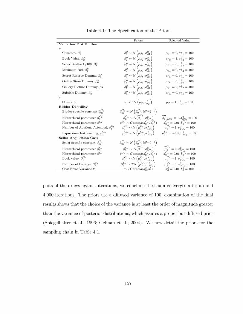
Table 4.1: The Specification of the Priors
Priors Selected ValueValuation Distributionµ
Constant, βµ1 βµ1 ∼ N“µβ1 , σ
2β1
”µβ1 = 0, σ2
β1 = 100
Book Value, βµ2 βµ2 ∼ N“µβ2 , σ
2β2
”µβ2 = 1, σ2
β2 = 100
Seller Feedback/100, βµ3 βµ3 ∼ N“µβ3 , σ
2β3
”µβ3 = 0, σ2
β3 = 100
Minimum Bid, βµ4 βµ4 ∼ N“µβ4 , σ
2β4
”µβ4 = 0, σ2
β4 = 100
Secret Reserve Dummy, βµ5 βµ5 ∼ N“µβ5 , σ
2β5
”µβ5 = 0, σ2
β5 = 100
Online Store Dummy, βµ6 βµ6 ∼ N“µβ6 , σ
2β6
”µβ6 = 0, σ2
β6 = 100
Gallery Picture Dummy, βµ7 βµ7 ∼ N“µβ7 , σ
2β7
”µβ7 = 0, σ2
β7 = 100
Subtitle Dummy, βµ8 βµ8 ∼ N“µβ8 , σ
2β8
”µβ8 = 0, σ2
β8 = 100
σ
Constant σ ∼ TN“µσ , σ2
σµ
”µσ = 1, σ2
σµ= 100
Bidder Disutility
Bidder specific constant βCb0j β
Cb0j ∼ N
“βCb0 , (φCb )−1
”Hierarchical parameter β
Cb0 β
Cb0 ∼ N(β
Cb
0 , σ20Cb
) β0
bidder = 1, σ20Cb
= 100
Hierarchical parameter φCb φCb ∼ Gamma(aCb0 , b
Cb0 ) a
Cb0 = 0.01, b
Cb0 = 100
Number of Auctions Attended, βCb1 β
Cb1 ∼ N
“µCb1 , σ2
1Cb
”µCb1 = 1, σ2
1Cb= 100
Lapse since last winning, βCb2 β
Cb2 ∼ N
“µCb2 , σ2
2Cb
”µCb2 = −0.5, σ2
2Cb= 100
Seller Acquisition Cost
Seller specific constant βCs0i βCs
0i ∼ N“βCs0 , (φCs )−1
”Hierarchical parameter βCs
0 βCs0 ∼ N(β
Cs
0 , σ20Cs
) βCs
0 = 0, σ20Cs
= 100
Hierarchical parameter φCs φCs ∼ Gamma(aCs0 , bCs
0 ) aCs0 = 0.01, b
Cb0 = 100
Book value, βCs1 βCs
1 ∼ N“µCs
1 , σ21Cs
”µCs
1 = 1, σ21Cs
= 100
Number of Listings, βCs2 βCs
2 ∼ TN“µCs
2 , σ22Cs
”µCs
2 = 3, σ22Cs
= 100
Cost Error Variance θ θ ∼ Gamma(aθ0, bθ0) aθ0 = 0.01, bθ0 = 100
plots of the draws against iterations, we conclude the chain converges after around
4,000 iterations. The priors use a diffused variance of 100; examination of the final
results shows that the choice of the variance is at least the order of magnitude greater
than the variance of posterior distributions, which assures a proper but diffused prior
(Spiegelhalter et al., 1996; Gelman et al., 2004). We now detail the priors for the
sampling chain in Table 4.1.
157
The Conditional Posterior for the Seller Acquisition Costs: βCs0i , βCs0 , φCs , βCs1 , βCs2 ,
θ and πit
• LetXqit (qit) = BOOKV ALβCs1it q
βCs2it , Yqit (qit) = qit·(1−commission)E(Rs
itn|·)−
qit · feeit and εqit = −eCsqit . Then equation (1.12) can be written as
πit(qit) = qit · (1− commission)E(Rsitn|·)− Cs
it(qit)− qit · feeit (4.6)
= Yqit (qit)− βCs0i Xqit(qit) + εqit
Similarly, for a deviation from qit, the profit would be
πit(qit) = qit · (1− commission)E(Rsitn|·)− Cs
it(qit)− qit · feeit (4.7)
= Yeqit (qit)− βCs0i Xeqit(qit) + εeqitFor each iteration through the sampling chain, a set of latent π (qit) will be
drawn from a normal distribution with mean Yqit (qit) − βCs0i Xqit(qit) and vari-
ance (θ)−1. A set of deviated profits π (qit) will be drawn from a truncated
normal distribution with mean Yeqit (qit)−βCs0i Xeqit(qit), variance (θ)−1 and right
truncation at π (qit). We consider 20 such qit and have found results to be
robust to this choice.
158

• βCs0i
Prior βCs0i ∼ N(βCs0 , (φCs)−1
)(4.8)
Likelihood L ∝Ti,eqit 6=qit∏
exp
(−[πit(qit)−
(Yeqit − βCs0i Xeqit)]2 θ
2
)Ti,qit∏
exp
(−[πit(qit)−
(Yqit − βCs0i Xqit
)]2θ
2
)
exp
(−(βCs0i − βCs0
)2φCs
2
)(4.9)
Posterior (βCs0i |·) ∼ N(µCsi , ΣCsi ) (4.10)
ΣCsi = [(Xqi,eqi)′ (Xqi,eqi) θ + φCs ]−1 (4.11)
µCsi = ΣCsi [(Xqi,eqi)′ (πi(qi , qi)− Yqi,eqi) θ + βCs0 φCs ] (4.12)
where Ti is the total number of items listed by seller i; (Xqi,eqi) is the vector
containing Xqit and Xeqit of seller i; (πi(qi , qi)− Yqi,eqi) is a vector containing all
(πit(qit)− Yqit) and (πit(qit)− Yeqit) of seller i.
• βCs0
Prior βCs0 ∼ N(βCs
0 , σ20Cs) (4.13)
Likelihood L ∝I∏i=1
exp
(−(βCs0i − βCs0
)2φCs
2
)(4.14)
Posterior (βCs0 |·) ∼ N(λCs ,ΛCs) (4.15)
ΛCs = [σ−20Cs
+ φCs ]−1 (4.16)
λCs = ΛCs [∑i
βCs0i φCs + β
Cs
0 /σ20Cs ] (4.17)
where I is the total number of sellers observed.
159

• φCs
Prior φCs ∼ Gamma(aCs0 , bCs0 ) (4.18)
Likelihood L ∝I∏i=1
(φCs)1/2
exp
(−(βCs0i − βCs0
)2φCs
2
)(4.19)
Posterior (φCs |·) ∼ Gamma(aCs , bCs) (4.20)
aCs = I/2 + aCs0 (4.21)
bCs = 2bCs0 [2 + bCs0 · s]−1 (4.22)
s =I∑i=1
(βCs0i − βCs0
)2(4.23)
• An updated βCs(k)1 in the k−th iteration is obtained with a random walk pro-
posal density. For this we use a normal distribution with mean of βCs(k−1)1 from
last iteration, variance σβCs1. The value of σβCs1
is determined such that the
acceptance rate of proposed values is between 15%-50% (Roberts, 1996). The
proposed βCs(k)1 is accepted with the probability of κ∗ = min1, κ, where
κ =L(β
Cs(k)1 |·)p
(βCs(k)1 |µCs1 , σ2
1Cs
)L(β
Cs(k−1)1 |·)p
(βCs(k−1)1 |µCs1 , σ2
1Cs
) (4.24)
L(βCs(·)1 |·) denotes the conditional likelihood and
L(βCs(·)1 |·) ∝
∏t,i,eqit 6=qit
exp
(−[πit(qit)−
(Yeqit − βCs0i Xeqit)]2 θ
2
)(4.25)
∏t,i
exp
(−[πit(qit)−
(Yqit − βCs0i Xqit
)]2θ
2
)(4.26)
p(βCs(·)1 |µCs1 , σ2
1Cs
)is the prior density evaluated at β
Cs(·)1 .
160

• An updated βCs(k)2 in the k−th iteration is obtained with a random walk pro-
posal density. For this we use a truncated normal distribution with mean of
βCs(k−1)2 from last iteration, variance σβCs2
and left truncated at 1. The value of
σβCs2is determined such that the acceptance rate of proposed values is between
15%-50% (Roberts, 1996). The proposed βCs(k)2 is accepted with the probability
of κ∗ = min1, κ, where
κ =L(β
Cs(k)2 |·)p
(βCs(k)2 |µCs2 , σ2
2Cs
)ρ(β
Cs(k−1)2 |βCs(k)2 , σβCs2
)
L(βCs(k−1)2 |·)p
(βCs(k−1)2 |µCs2 , σ2
2Cs
)ρ(β
Cs(k)2 |βCs(k−1)
2 , σβCs2)
(4.27)
where L(βCs(·)2 |·) denotes the conditional likelihood and
L(βCs(·)2 |·) ∝
∏t,i,eqit 6=qit
exp
(−[πit(qit)−
(Yeqit − βCs0i Xeqit)]2 θ
2
)(4.28)
∏t,i
exp
(−[πit(qit)−
(Yqit − βCs0i Xqit
)]2θ
2
)(4.29)
p(βCs(·)2 |µCs2 , σ2
2Cs
)is the prior density evaluated at β
Cs(·)2 .
ρ(·|·) represents the density of the proposal distribution evaluated with
βCs(k)2 , β
Cs(k−1)2 , σβCs2
as input and parameters. For example, ρ(βCs(k−1)2 |βCs(k)2 , σβCs2
) is the density
evaluated at βCs(k−1)2 with β
Cs(k)2 and σβCs2
as mean and variance, respectively.
Note that since the proposal distribution is truncated at 1 and thus asymmetric,
the ratio between the two densities is used as a weight to obtain the correct
acceptance probability.
161

• θ
Prior θ ∼ Gamma(aθ0, bθ0) (4.30)
Likelihood L ∝∏
i,t,eqit 6=qit(θ)1/2 exp
(−[πit(qit)−
(Yeqit − βCs0i Xeqit)]2 θ
2
)
∏i,t
(θ)1/2 exp
(−[πit(qit)−
(Yqit − βCs0i Xqit
)]2θ
2
)
Posterior (θ|·) ∼ Gamma(aπ, bθ0) (4.31)
aπ = IT(Q+ 1
)/2 + aθ0 (4.32)
bθ0 = 2bθ0[2 + bθ0 · s]−1 (4.33)
s =∑
i,t,eqit 6=qit[πit(qit)−
(Yeqit − βCs0i Xeqit)]2 (4.34)
+∑i,t
[πit(qit)−
(Yqit − βCs0i Xqit
)]2(4.35)
The Conditional Posterior for the Bidder Valuation Model, βµ, µ, σ, v∗ijtn|Ibid
• βµ
Prior: βµ ∼ N(µβµ ,Σβµ) (4.36)
Likelihood L ∝∏i,t,n
exp
(−(µit − Zµ
itβµ)2
2
)(4.37)
Posterior: (βµ|·) ∼ N(µβµ , Σβµ) (4.38)
with Σβµ = Σ−1βµ + Zµ′ · Zµ−1 (4.39)
µβµ = ΣβµZµ′ · µ+ Σ−1βµµβµ (4.40)
162

where µβµ is a column vector of dimension 8 containing all prior means for βµ; Σβµ
is a 8× 8 matrix with the prior variances of βµ on the diagonal and 0 as off-diagonal
elements; µ is a column vector of the µit across itn with a dimension of ITN ; Zµ is a
the matrix in the dimension of ITN×8, containing independent variables determining
the valuation distribution mean, µ.
• v∗ijtn|Ibid
For observations where Ibid = 0 (see Section (1.4.1)), Theorem 1.1 indicates that
v∗ijtn is drawn from a right truncated N(µit, σ) with truncation level x∗ijtn. This
becomes the v∗ijtn for all subsequent items of the same type.
• µ and σ
There is no closed form density for the conditional posterior of µit so we use a
random walk Metropolis algorithm to obtain updated draws through the MCMC
chain. A normal distribution is used as the proposal density. The proposal density
has mean µ(k−1)it from (k − 1)−th iteration and a variance of Σµ. The value of Σµ is
determined such that the acceptance rate of proposed values is between 15%-50%.
With the proposal density, an updated value is generated and denoted as µ(k)it .
The proposed µ(k)it is accepted with the probability κ∗, where
κ∗ = min1, κ
κ =L(µ
(k)it |·)
L(µ(k−1)it |·)
(4.41)
where the conditional likelihood
L(µ(·)it |·) ∝ LbidderLsellerp(µit|Zµ
it, βµ) (4.42)
L(µ(k)it |·) denotes the conditional likelihood evaluated at µ
(k)it and L(µ
(k−1)it |·) is
the analogy.
163

For the sampling of an updated σ, a truncated normal distribution is used as the
proposal density as the variance must be positive. The proposal density has mean
σ(k−1), variance Σσ and left truncated at zero.
κ∗ = min1, κ
κ =L(σ(k)|·)p
(σ(k)|µσ, σ2
σµ
)ρ(σ(k−1)|σ(k),Σσ)
L(σ(k−1)|·)p(σ(k−1)|µσ, σ2
σµ
)ρ(σ(k)|σ(k−1),Σσ)
(4.43)
where the conditional likelihood
L(σ(·)|·) ∝ LbidderLseller (4.44)
L(σ(k)|·) is the posterior likelihood evaluated at σ(k) and L(σ(k−1)|·) is the analog for
σ(k−1). p(σ(k)|µσ, σ2
σµ
)is the prior density evaluated at σ(k) and p
(σ(k−1)|µσ, σ2
σµ
)is
the analog for σ(k−1). ρ(·|·) represents the density of the proposal distribution evalu-
ated with σ(k), σ(k−1) and Σσ as input and parameters. For example, ρ(σ(k−1)|σ(k),Σσ)
is the density evaluated at σ(k−1) with σ(k) and Σσ as mean and variance, respectively.
Note that since the proposal distribution is truncated at zero and thus asymmetric,
the ratio between the two densities is used as a weight to obtain the correct accep-
tance probability.
164

The Conditional Posterior for the Bidder Cost Model, βCb0j , βCb0 , φCb , βCb and Cbijtn
• βCb0j
Prior βCb0j ∼ N(βCb0 , (φCb)−1
)(4.45)
Likelihood L ∝∏itn
exp
−(logCb
ijtn − βCb0j − ZCb
ijtnβCb)2
2
(4.46)
Posterior (βCb0j |·) ∼ N(µCbj , ΣCbj ) (4.47)
ΣCbj = [ITN + φCb ]−1 (4.48)
µCbj = ΣCbj [1′ITN
(Cbj − ZCb
j βCb)
+ βCb0 φCb ] (4.49)
where ITN is the total number of auctions across itn; Cbj is the vector of
the latent (log) costs of bidder j, having a length of ITN ; ZCb
j is an 2 ∗ ITN
matrix containing AttendedAuction and Lapse; βCbis the vector of parameters
associated with ZCb
j ; 1′ITN is a vector of 1’s with the length of ITN ;and
var(logCbijtn) = 1.
• βCb0
Prior βCb0 ∼ N(βCb
0 , σ20Cb
) (4.50)
Likelihood L ∝J∏J=1
exp
−(βCb0j − βCb0
)2
φCb
2
(4.51)
Posterior (βCb0 |·) ∼ N(λCb ,ΛCb) (4.52)
ΛCb = [σ−20Cb
+ φCb ]−1 (4.53)
λCb = ΛCb [∑j
βCb0j φCb + β
Cb
0 /σ20Cb
] (4.54)
165

where J is the total number of bidders observed.
• φCb
Prior φCb ∼ Gamma(aCb0 , bCb0 ) (4.55)
Likelihood L ∝J∏j=1
(φCb)1/2
exp
−(βCb0j − βCb0
)2
φCb
2
(4.56)
Posterior (φCb|·) ∼ Gamma(aCb , bCb) (4.57)
aCb = J/2 + aCb0 (4.58)
bCb = 2bCb0 [2 + bCb0 · s]−1 (4.59)
s =J∑j=1
(βCb0j − βCb0
)2
(4.60)
• βCb
Prior: βCb ∼ N
(µCb ,ΣCb
)(4.61)
Likelihood L ∝∏ijtn
exp
−(logCb
ijtn − βCb0j − ZCb
ijtnβCb
)2
2
(4.62)
Posterior: (βCb|·) ∼ N(µβCb , ΣβCb ) (4.63)
with ΣβCb = Σ−1Cb
+ ZCb′ · ZCb−1 (4.64)
µβCb = ΣβCbZCb′ ·(Cb − βCb0
)+ Σ−1
Cs× µCb (4.65)
where ZCb is a matrix containing all the ZCb
ijtn across ijtn and is dimensioned
IJTN by 2; Cb is a column vector containing all log bidder costs across ijtn with a
length of IJTN ; βCb0 is a column vector with a length of IJTN (where βCb0 can be
construed as J stacked sub-vectors where the j−th sub-vector has dimension ITN
166

and βCb0j as its elements); µCb is a 2 by 1 vector of whose elements contain the prior
means for parameters corresponding to ZCb (AttendedAuction and Lapse); and ΣCb
is a 2 by 2 matrix whose diagonal elements contain the prior variances and whose
off-diagonals are zeroes.
• Cbijtn
An updated Cb(k)ijtn in the k−th iteration is obtained with a random walk proposal
density with mean Cb(k)ijtn from iteration k − 1 and variance σCb . The candidate draw
Cb(k)ijtn is accepted with the probability of κ∗ = min1, κ, where
κ =L(C
b(k)ijtn |·)ρ(C
b(k−1)ijtn |Cb(k)
ijtn , σCb)
L(Cb(k−1)ijtn |·)ρ(Cb(k)
ijtn |Cb(k−1)ijtn , σCb)
(4.66)
where L(Cb(·)ijtn|·) denotes the conditional likelihood and
L(Cb(·)ijtn|·) ∝ LbidderLsellerp(Cb
ijtn|βCb0j , Z
Cb
ijtn, βCb) (4.67)
Thus, L(Cb(·)ijtn|·) is the conditional likelihood evaluated at C
b(k)ijtn and L(C
b(k−1)ijtn |·) is
the analog at iteration k − 1.3
ρ(·|·) connotes the density of the proposal distribution evaluated with Cb(k)ijtn ,
Cb(k−1)ijtn , and σCb as inputs. As the proposal distribution is truncated and asymmetric,
the ratio between the two densities of ρ(Cb(k−1)ijtn |Cb(k)
ijtn , σCb) and ρ(Cb(k)ijtn |C
b(k−1)ijtn , σCb)
is used as a weight to obtain the correct acceptance probability.
4.1.4 Monte Carlo Simulation
We develop a simulated data set designed to reflect our model and data in order
to assess whether the proposed estimation approach can recover true parameters
3 Note that a seller makes decision in Stage 1 before bidder’s decisions. The seller takes the biddercosts distribution into account when he calculates the expected return. Thus Lseller also appearsin the conditional likelihood of Cb
ijtn
167

for an arbitrary set of values. The simulated data have 10 sellers and 100 bidders.
Each seller has 2-4 items for sale and makes decisions about the optimal number of
auctions for each item. The sellers’ optimization results in a total of 213 auctions
in the market. Each bidder then makes decisions about bidding activities. The true
values and estimates of parameters are presented in Table 4.2 and indicate that the
model is capable of recovering parameters with reasonable accuracy.
Table 4.2: Monte Carlo Simulation Results
True Value Median 95% IntervalsValuation Distributionµ
Constant -4 -3.89* (-4.18, -3.51)Book Value 1 0.99* (0.83, 1.15)(Seller Feedback) 0.5 0.49* (0.06, 0.89)Minimum Bid 0.5 0.51* (0.09, 0.91)Secret Reserve Dummy 0.5 0.49* (0.25, 0.72)Store Dummy 0.5 0.50* (0.29, 0.75)Gallery Picture 0.5 0.50* (0.24, 0.72)Subtitle 0.5 0.51* (0.32, 0.67)
σConstant 2 2.09* (1.98, 2.20)
Bidder DisutilityNumber of Auctions Attended 1 0.99* (0.96, 1.02)Lapse Since Last Winning -0.4 -0.39* (-0.37, -0.41)Mean of the Individual Constant 2 2.08* (1.36, 2.83)
Seller Acquisition CostBook Value 1 0.99* (0.94, 1.05)Number of Listings 1.5 1.51* (1.44, 1.55)Cost Error Variance 1 1.10* (0.91, 1.22 )Mean of the Individual Constant 0.50 0.56* (0.36, 0.88)
168

4.2 Appendices for “A Dynamic Model of Sponsored Search Adver-tising”
4.2.1 Two Step Estimator
First Step Estimation
Estimating the Advertiser’s Policy Function
The Partial Policy Function The partial policy function links states (s) and char-
acteristics (X) to decisions (b). Ideally this relation can be captured by a relatively
flexible parametric form and estimated via methods such as maximum likelihood or
MCMC to obtain the partial policy function parameter estimates. The exact func-
tional form is typically determined by model fit comparison among multiple speci-
fications (e.g. Jofre-Bonet and Pesendorfer, 2003). We considered several different
specifications for the distribution of bids and found the truncated normal distribution
gives the best fit in terms of marginal likelihoods.4 Specifically, we allow
btj =
yt∗j0
if yt∗j ≥ χotherwise
(4.68)
yt∗j ∼ N([st′,Xt′j ] · ϕ+ ϕj, τ
2)
where [st′,Xt′j ] is the vector of independent variables; τ is the standard deviation
of y∗jt; ϕj is a bidder specific constant term due to the fixed effect fj in valuations
(equation 2.15); and χ is the truncation point, which is set at 15 to be consistent
with the 15c minimum bid requirement of the search engine.
One possible concern when estimating the partial policy function σ (s,X) (and
the full policy function σ(s,X, rtj
)next) is that there may be multiple equilibrium
strategies; and the observed data are generated by multiple equilibria. If this were
4 We experimented with alternative specifications including a Beta distribution and a Weibulldistribution whose scale, shape, and location parameters are functions of (s,X). The currentspecification gives the best fit in terms of marginal likelihoods.
169

the case, the policy function would not lead to a unique decision and would be of
limited use in predicting advertiser behavior. It is therefore necessary to invoke the
following assumption (BBL).
Assumption 2 (Equilibrium Selection): The data are generated by a single
Markov perfect equilibrium profile σ.
Assumption 2 is relatively unrestrictive since our data is generated by auctions of one
keyword and from one search engine. Given data are from a single market, the like-
lihood is diminished that different equilibria from different markets are confounded.
We note that this assumption is often employed in such contexts (e.g., Dube et al.,
2008).
This partial policy function is then used to impute the full policy function bj =
σj(s,X, rtj
)as detailed below based on rtj’s distribution parameter ψ.
Full Policy Functions σtj
(st,Xt,rtj
)To evaluate the value function of this dynamic
game, we need to calculate bids as a function of not only (st,Xt) but also the un-
observed shocks rtj (see section 2.4.2). To infer this full policy function σj(st,Xt,rtj
)from the estimated partial policy function, σj(s
t,Xt), we introduce one additional
assumption.
Assumption 3 (Monotone Choice): For each bidder j, its equilibrium strategy
σj(st,Xt,rtj
)is increasing in rtj (BBL).
Assumption 3 implies that bidders who draw higher private valuation shocks rtj will
bid more aggressively.
To explore these two assumptions, note that the partial policy function σ(st,Xt
)presents distributions for bid btj and the latent yt∗j , whose CDF’s we denote as
Fb(btj|st,Xt
)and F
(yt∗j |st,Xt
), respectively.5 According to the model in equation
5 To be more specific, we estimate a continuous distribution F(yt∗
j |st,Xt)
for yt∗j from equation
4.68; then conditional on the trunction point χ, we can back out the (discontinuous) distribution
170

4.68, the population mean of yt∗j across bidders and periods is [st,Xtj]·ϕ+ϕj. Around
this mean, the variation across bidders and periods can be captured by the variance
term τ 2. With assumption 3, we can attribute τ 2 to the random shocks rtj.
Given the normal distribution assumption of the random shock rtj ∼ N (0, ψ2),
we may impute the yt∗j (and hence btj) for each combination of(st,Xt,rtj
), i.e., the
full policy function. To see this, note that since σj(st,Xt,rtj
)is increasing in rtj,
6
F(yt∗j |st,Xt
)= Pr
(σj(st,Xt,rtj
)≤ yt∗j |st,Xt
)= Φ
(σ−1j
(yt∗j , s
t,Xt)/ψ)
where σ−1j
(yt∗j , s
t,Xt)
is the inverse function of σj(st,Xt,rtj
)with respect to rtj
and Φ(·) is the CDF of standard normal distribution. In equilibrium, we have
σj(st,Xt,rtj
)= yt∗j . By substitution and rearrangement we get
yt∗j = σj(st,Xt,rtj
)(4.69)
= F−1(Φ(σ−1j
(yt∗j , s
t,Xt)/ψ)|st,Xt
)= F−1
(Φ(rtj/ψ
)|st,Xt
)where σ−1
j
(yt∗j , s
t,Xt)
= rtj; rtj/ψ has a standard normal distribution.
Therefore there is a unique mapping between the likelihood of observing a given
valuation shock rtj and the yt∗j . Each rtj drawn by a firm implies a corresponding
quantile on the rtj’s distribution; this quantile in turn implies a yt∗j from the distribu-
tion represented by that firm’s partial bidding function σj(st, X t). However, because
Fb
(btj |st,Xt
)for bt
j .6 In this Appendix, we are abusing the notation of σj
(st,Xt,rt
j
). For the purpose of a clear
exposition, we define σj
(st,Xt,rt
j
)= bt
j in the paper. To match the bidding function estimated inequation 4.68, the more accurate definition should be
btj =
yt∗
j
0if yt∗
j ≥ χotherwise
yt∗j = σj
(st,Xt,rt
j
)
171

we do not know ψ and, thus, the distribution of rtj, we have to make draws from an
alternative distribution rtj/ψ that has a one-one quantile mapping to rtj. To do this,
we first draw a random shock rtj/ψ from N(0, 1) for each advertiser i in period t.
Next, we determine F(yt∗j |st,Xt
)using results estimated in 4.68 and looking at the
distribution of its residuals to determine F . That is, for each value of yt∗j , we should
be able to compute its probability for a given st and Xt using F . Accordingly, F−1
links probabilities to yt∗j (therefore btj) for a given st and Xt. We then use F−1 to
link the probability Φ(rtj/ψ
)to btj for a particular st and Xt. In this manner we
ensure the bids and valuations in equation (4.78) comport. In Appendix 4.2.1, when
evaluating the value function for a set of given parameter values of ψ in equation
4.78 or evaluating base functions defined in equation 4.79, we integrate out over the
unobserved shocks rtj by drawing many rtj/ψ from N(0, 1).
Consumer Model Estimation We derive the consumer model conditioned on the in-
formation state of the advertiser as described in section 2.4.1. Given that advertisers
do not observe what each person downloaded or the characteristics of these persons,
they must infer consumer behavior from aggregate instead of individual level data.
Advertisers do observe the aggregate data in the form of download counts dtj =
dt1, dt2, ..., dtN in period t. A single dtj follow a binomial distribution. Given the
download probabilities P tj in equation 2.12, a single dtj’s probability mass function is(
Mt
dtj
)[P tj ]dtj [1 − P t
j ]Mt−dtj , where Mt is the consumer population size in period t.
Hence the likelihood of observing dt is
L(dt|Ωc) =∏
j
(Mt
dtj
)[P tj ]dtj [1− P t
j ]Mt−dtj
where Ωc ≡ αg, βg, δg, γg, λg0, λg1g are parameters to be estimated.
Naturally, the full posterior distribution of the model will be the product of
172

L(dt|Ωc) across periods and p(Ωc), the prior distributions of parameters, i.e.,
p(Ωc|data) ∝∏t
L(dt|Ωc) · p(Ωc) (4.70)
An advertiser’s predicted downloads dtj(k,Xtj ; Ωc) can readily be constructed us-
ing the parameter estimates as shown in equation 2.13
dtj(k,Xtj ; Ωc) = MtP
tj (4.71)
This prediction is then used to forecast expectations of future downloads and slot
positions in the firm’s value function in the second step estimation.
State Transition Function P(s′ |bj ,b−j , s,X
)To compute the state transition, note
that the marginal number of expected downloads is given by the expected downloads
given a slot position multiplied by the probability of appearing in that slot position
and then summed across all positions:
P(s′|bj,b−j, s,X
)=∑
kd(k,X; Ωc) Pr (k|bj,b−j, s,X) (4.72)
The expected downloads given a slot position in 4.72 is defined in 2.13. We can
decompose the likelihood of appearing in slot k as follows
Pr(k|bj,b−j, s,X) (4.73)
= Prk≤K (k|bj,b−j, s,X) Ik ≤ K+ Prk>K(k|bj,b−j, s,X)Ik > K
where Prk≤K (k|bj,b−j, s,X) is the probability of appearing in slot k of the spon-
sored search section (i.e., k ≤ K), and Prk>K(k|bj,b−j, s,X) is the likelihood of
appearing in slot k of the organic search section (i.e., k > K). We discuss these two
probabilities next.
173

Likelihood of Premium Slot k ≤ K Let us first consider the likelihood of winning
one of the premium slots k (k ≤ K), Prk≤K (k|bj,b−j, s,X) as an order statistic re-
flecting the relative quality of the advertiser’s bid, which is defined as bjd(−1)j . Higher
quality bids are more likely to be assigned to better slots. Denote Ψbd(bj′d(−1)j′ |s,X)
as the distribution CDF of bj′d(−1)j′ ,∀j′, where d
(−1)j′ is from the state vector and bj′
has a distribution depending on the strategy profile σ (·).7 For bidder j to win a
premium slot k by bidding bj, it implies that (1) among all of the other N − 1 com-
peting bidders, there are k − 1 bidders who have a higher ranking than j in terms
of bj′d(−1)j′ and (2) the other ones have a lower ranking than j. The probability of
having a higher ranking than j is [1 − Ψbd(bjd(−1)j |s,X)]. Thus the probability of
bidder j winning slot k by bidding bj is simply an order statistics as shown below;
note that the combination
(N − 1k − 1
)in the equation is because any (k − 1) out of
the (N − 1) competing bidders can have a higher ranking than j.8
Prk≤K (k|bj,b−j, s,X) (4.74)
=
(N − 1k − 1
)[1−Ψbd(bjd
(−1)j |s,X)]k−1[Ψbd(bjd
(−1)j |s,X)](N−1)−(k−1)
=
(N − 1k − 1
)[1−Ψbd(bjd
(−1)j |s,X)]k−1[Ψbd(bjd
(−1)j |s,X)]N−k
Likelihood of Organic Slot k > K Next we consider what happens when an ad-
vertiser does not win this auction and is placed in the organic search section. In
this case, by the rules of the auction, the bidder’s slot is determined by its update
7 It is difficult to write a closed form solution for Ψbd, but we may use the sample populationdistribution to approximate Ψbd.
8 An alternative interpretation of equation 4.74 is the probability mass function (PMF) of abinomial distribution. Among N − 1 competing bidders, there are k − 1 higher than bidder j and(N −1)− (k−1) lower than j; and the probability of higher than j is [1−Ψbd(bjd
(−1)j |s,X)]. Hence
we may consider the expression in 4.74 as the PMF of a binomial distribution.
174

recency compared to all products in the organic search section. For bidder j to be
placed in organic slot k > K it implies that (1) there are K bidders who have a
higher ranking of bj′d(−1)j′ than bidder j (i.e., j loses the auction) and (2) among the
other N −K − 1 products (i.e., all products at the search engine less those who win
premium slots and j itself), there are k−K − 1 products that have a higher update
recency than j and (3) the other ones have a lower ranking than j. Hence,
Prk>K(k|bj,b−j, s,X)
= Pr(k > K|bj,b−j, s,X) · Pr(k|bj,b−j, s,X, k > K) (4.75)
where the first term is the probability of losing the auction (condition 1) and the
second term denotes the likelihood of appearing in position k > K (condition 2 and
3). Note that the main reason for the difference between 4.74 and 4.75 is the change of
ranking mechanisms. The ranking is based on bj′d(−1)j′ for k ≤ K and update recency
when k > K. The first term in 4.75 does not appear as an order statistics (as shown
below) since when k > K the order of bj′d(−1)j′ becomes meaningless. Instead, the
update recency is affecting the ranking. The two terms in 4.75 can be expressed as
follows.
Losing the auction implies that among j’s N − 1 opponents, there are K bidders
who have a higher ranking than j in terms of bj′d(−1)j′ . Hence,
Pr(k > K|bj,b−j, s,X) =
(N − 1K
)[1−Ψbd(bjd
(−1)j |s,X)]K (4.76)
The conditional probability of being placed in an organic slot k > K (condition
2 and 3) is, again, an order statistics.9 This distribution is incumbent upon the
update recency of all N products exclusive of the K winners in the sponsored search
9 This order statistics can, again, be interpreted as the PMF of a binomial distribution similar to4.74.
175

section. Denoting the distribution of update recency of all products as Ψup, which
can be approximated from the sample population distribution observed in the data,
we obtain the following:
Pr(k|bj,b−j, s,X, k > K) (4.77)
=
(N −K − 1k −K − 1
)[1−Ψup]
k−K−1[Ψup](N−K−1)−(k−K−1)
=
(N −K − 1k −K − 1
)[1−Ψup]
k−K−1[Ψup]N−k
Combining equations 4.77 and 4.76 into 4.75, and then 4.75 and 4.74 into 4.73,
yields the state transition equation.
Given that we have detailed the estimation of the first step functions (σj(s,X, rtj
),
dtj(k,Xtj ; Ωc), P (s′|b, s,X)), we now turn to the second step estimator, which is
incumbent upon these first step functions.
Second Step Estimation of Bidder Model
In this Appendix we detail how to estimate the parameters in the value function. This
is done in two phases; first, we simulate the value function conditioned on Ωa, and
second, we construct the likelihood using the simulated value function conditioned
on Ωa.
Phase 1: Simulation of Value Functions Given Ωa To construct the value function we
first simplify its computation by linearization, and second using this simplification,
we simulate the expected value function conditioned on Ωa by integrating out over
draws for st, Xt, and rtj.
Linearize the Value Function We simplify the estimation procedure by relying on
the fact that equation 2.16 is linear in the parameters Ωa. We can rewrite equation
176

2.16 by factoring out Ωa.
Eπj(bt, st,Xt, rtj; Ωa
)(4.78)
=∑K
k=1Pr(k|btj,bt−j, st,Xt
)· (v(X t
j ; θ) + fj + rtj − btj) · dtj(k,X tj ; Ωc)
+∑N
k=K+1Pr(k|btj,bt−j, st,Xt
)· (v(X t
j ; θ) + fj + rtj) · dtj(k,X tj ; Ωc)
=
[∑N
k=1Pr(k|btj,bt−j, st,Xt
)· dtj(k,X t
j ; Ωc) ·X tj
]· θ
+
[∑N
k=1Pr(k|btj,bt−j, st,Xt
)· dtj(k,X t
j ; Ωc)
]· fj
+
[∑N
k=1Pr(k|btj,bt−j, st,Xt
)· dtj(k,X t
j ; Ωc) · rtj]· ψ
−btj∑K
k=1Pr(k|btj,bt−j, st,Xt
)dtj(k,X
tj ; Ωc)
= Basetj1[θ′, fj]
′ +Basetj2ψ −Basetj3
where
Basetj1 ≡
[ ∑Nk=1 Pr
(k|btj,bt−j, st,Xt
)· dtj(k,X t
j ; Ωc) ·X tj∑N
k=1 Pr(k|btj,bt−j, st,Xt
)· dtj(k,X t
j ; Ωc)
]′(4.79)
Basetj2 ≡[∑N
k=1Pr(k|btj,bt−j, st,Xt
)· dtj(k,X t
j ; Ωc) · rtj]
Basetj3 ≡ btj∑K
k=1Pr(k|btj,bt−j, st,Xt
)dtj(k,X
tj ; Ωc)
rtj = rtj/ψ ∼ N(0, 1)
Note that the values ofBasetj1, Base
tj2, Base
tj3
∀t are conditionally independent
of θ, fj and ψ. This enables us to first evaluateBasetj1, Base
tj2, Base
tj3
∀t and keep
them constant when drawing θ, fj and ψ from their posterior distributions. By doing
so, we reduce the computational burden of estimation as described next.
177

Simulate the Value Functions Given Ωa After the linearization, given a set of ad-
vertiser parameters Ωa = θ, fj=1,2,...,N , ψ and equation 4.78, the value function
depicted in equation 2.18 can also be written as the following with period index t
invoked:
Vj(s0,X0;σ; Ωa
)= Es,X,r
[∞∑t=0
ρtπj(σ, st,Xt, rtj; Ωa
)](4.80)
= E[∞∑t=0
(ρtBasetj1
[θfj
]+Basetj2ψ −Basetj3)]
= [E∞∑t=0
ρtBasetj1]
[θfj
]+ [E
∞∑t=0
ρtBasetj2]ψ − [E∞∑t=0
ρtBasetj3]
where the expectation is taken over current and future private shocks, future states
st, future Xt and Rt.
An estimated value function Vj (s0,X0;σ; Ωa) can then be obtained by the fol-
lowing steps:
1. Draw private shocks rtj from N(0, 1) for all bidders j in period 0; draw initial
choice of s0 from the distribution of state variables derived from the observed
data; draw X0 from the observed distribution of product attributes.
2. Starting with the initial state s0, X0 and the rtj step 1, calculate b0j for all
bidders using the inversion (equation 4.69) described in Appendix 4.2.1.
3. Use s0, X0 and b0 to determine the slot ranking, whose distribution is
Pr(k|btj,bt−j, st,Xt
)in equation 4.73 in Appendix 4.2.1; using d(k,X0
j ; Ωc) in equation 2.13, obtain
a new state vector s1, whose distribution is P (s1|b0, s0,X0) in equation 4.72 in
Appendix 4.2.1; draw X1 from the observed distribution of product attributes.
178
4. Repeat steps 1-3 for T periods for all bidders to compute all st, Xt, rtj, and bt
for all periods; T is large enough so that the discount factor ρT approaches 0.
5. Using st, Xt, rtj, dtj(k,X
tj ; Ωc), and bt, evaluate
Basetj1, Base
tj2, Base
tj3
t=0,...,T
and
[T∑t=0
ρtBasetj1], [T∑t=0
ρtBasetj2], [T∑t=0
ρtBasetj3]
.
6. The resulting values of
Basetj1, Base
tj2, Base
tj3
t=0,...,T
and [T∑t=0
ρtBasetj1], [T∑t=0
ρtBasetj2], [T∑t=0
ρtBasetj3]
depend on the random draws of st,Xt, rt. To compute
[E
∞∑t=0
ρtBasetj1], [E∞∑t=0
ρtBasetj2], [E∞∑t=0
ρtBasetj3]
,
repeat steps 1-6 for NR times so as to integrate out over the draws. Note that
when T is large enough [ET∑t=0
ρtBasetj·] is a good approximation of [E∞∑t=0
ρtBasetj·]
since ρT approaches 0.
7. Conditional on a set of parameters Ωa and
[E
∞∑t=0
ρtBasetj1], [E∞∑t=0
ρtBasetj2], [E∞∑t=0
ρtBasetj3]
,
we may evaluate Vj (s0,X0;σ; Ωa) from equation4.80.
An estimated deviation value function Vj(s0,X0;σ′j, σ−j; Ωa
)with an alternative
strategy σ′j other than σj can be constructed by following the same procedure. We
179

draw a deviated strategy σ′j by adding disturbance to the estimated policy function
from Step 1. In particular, we add a normally distributed random variable (mean =
0; s.d. = 0.3) to each parameter.
We implement this process by first drawing NS = 10 initial states for each bidder
and X tt=0,1,...,T of all T = 200 periods. Then for each combination of bidder and
initial state, we use this process to compute the base value functions and ND = 100
perturbed base functions. In Step 6, we use NR = 100. The discount factor ρ is
fixed as 0.95.
The computational burden is reduced tremendously since we have linearized the
value functions and factored out the parameters Ωa. We do not need to re-evaluate
the value functions for each set of parameters Ωa. Instead, we only evaluate the base
functions in equation 4.79 once using step 1-6 and keep them fixed. Then for each
draw of Ωa from the posterior distribution we may evaluate the value functions (step
7) so as to recover Ωa as described below.
Phase 2: Recover Ωa Recall our goal is to assess the likelihood that 2.19 holds. Define
Pj
(s0(ns),X
0;σ, σ′j; Ωa
)as the probability of the event
Vj(s
0(ns),X
0;σj, σ−j; Ωa) ≥ Vj(s0(ns),X
0;σ′j, σ−j; Ωa), (4.81)
where s0(ns) stands for the ns-th initial state of bidder j. This event means that the
estimated value function for the given initial state s0(ns) with observed strategy σj is
greater than the estimated value function with a deviation σ′j. For observed data to
be rational, we should have Pj
(s0(ns),X
0;σ, σ′j; Ωa
)converging to 1 under the true
parameters, in the sense that all ND draws should result in the event of equation
4.81.
Note that Pj
(s0(ns),X
0;σ, σ′j; Ωa
)is not observed, but it can be approximated
180

with the sample analog from the simulated ND draws of Vj(s0(ns), X
0;σ′j, σ−j; Ωa) as
the follows:
Pj(s0(ns),X
0;σ, σ′j; Ωa
)(4.82)
=1
ND
∑ND
nd=1IVj(s
0(ns),X
0;σj, σ−j; Ωa) ≥ Vj(s0(ns),X
0;σ′j, σ−j; Ωa)(nd)
where the subscript (nd) indices the nd-th simulated Vj(s
0(ns), X
0;σ′j, σ−j; Ωa).
By pooling together all Pj
(s0(ns),X
0;σ, σ′j; Ωa
)’s across bidders and (ns), we are
able to construct a simulated likelihood function as the following
L =∏
j,(ns)Pj(s0(ns),X
0;σ, σ′j; Ωa
)(4.83)
Denoting the prior of Ωa as p(Ωa), the posterior can be written as
p(Ωa|data) ∝∏
j,(ns)Pj(s0(ns),X
0;σ, σ′j; Ωa
)p(Ωa) (4.84)
There may be some efficiency loss by using Bayesian method in estimation since
the differences between Vj(s0(ns), X
0;σj, σ−j; Ωa) and Vj(s0(ns), X
0;σ′j, σ−j; Ωa) also pro-
vide some information about the estimates and are not utilized (BBL). However,
Bayesian method provides desirable small sample properties, increases statistical ef-
ficiency, and enables the estimation of a wide array of functional forms (Rossi et al.,
2005). We consider the benefits of Bayesian method to outweigh the loss of efficiency.
4.2.2 MCMC Sampling Chain
Advertiser Model
Priors The specification of advertiser model priors is listed in Table 4.3.
To facilitate explication denote the vector [st′,Xt′j ] ≡ Zt
j , the matrix [Ztj ]∀j,t ≡ Z
and the vector [yt∗j ]∀j,t ≡ y∗. We also denote the number of bidders as N and the
181

number of observations for bidder j as Nj. So the total number of observations is∑j Nj; the dimension of Zt
j is 1 by d (the dimension of [st′, X t′j ]); the dimension of
Z is∑
j Nj by d; and the dimension of y∗ is∑
j Nj. The vector of bidder specific
fixed effects, ϕfe, is a column vector with a length of the number of bidders. Λ is
a matrix whose dimension is∑
j Nj by N . Suppose rows a to b of matrix Z are
the observations of bidder j, then rows a to b of the j-th column of Λ are 1. Other
elements of Λ are 0. Also denote Γ ≡ [Λ, Z], whose dimension is∑
j Nj by (N + d).
The advertiser model is specified as
btj =
yt∗j0
if yt∗j ≥ χotherwise
(4.85)
yt∗j ∼ N([st′,Xt′j ] · ϕ+ ϕj, τ
2)
We iterate the sampling chain for 20,000 and use the second half of the chain to make
inference. The priors use a diffused variance of 100; examinations of the posteriors
shows that the choice of the variance is the order of magnitude greater than posterior
distributions, which assures a proper but diffused prior (Spiegelhalter et al., 1996;
Gelman et al., 2004).
Table 4.3: The Specification of the Priors for Advertiser Bidding Model
Priors Selected Value
ϕ =[ϕ′, ϕ1, ..., ϕN ]′ ϕ ∼ N`ϕ0, Iϕσ2
ϕ
´ ϕ0: estimates of a classical Tobit model ofbids on Γ = [Λ, Z] with the truncation at 15.σ2ϕ = 100Iϕ is an identity matrix with the dimension ofN + d.
τ τ ∼ TN(0,+∞)(µτ , σ2τ ) µτ = 5, σ2
τ = 100
Conditional Posteriors
• yt∗j
182
yt∗j is determined by the following
yt∗j = btj, if btj > 0
yt∗j ∼ TN(−∞,15](Ztjϕ+ ϕj, τ
2), if btj = 0
yt∗j is right truncated at 15 when btj = 0; this is consistent with the 15c minimum
bid requirement of the search engine.
• ϕ
Prior ϕ ∼ N(ϕ0, Iϕσ
2ϕ
)(4.86)
Likelihood L ∝∏j,t
exp(−[yt∗j − (Zt
jϕ+ ϕj)]2
2τ 2)
Posterior (ϕ|·) ∼ N(µϕ,Σϕ)
Σϕ = [Γ′Γτ−2 + σ−2ϕ ]−1
µϕ = Σϕ · Γ′ · y∗τ−2 + ϕ0σ−2ϕ
• τ
Prior τ ∼ TN(0,+∞)(µτ , σ2τ )
A random walk proposal density is used in the (r)-th iteration,
τ (r) ∼ TN(0,+∞)(τ(r−1), σ2
p)
where τ (r−1) is the value from the (r−1)-th iteration; σ2p is the tuning variance
which is chosen so that the acceptance rate is between 15%− 50%.
The acceptance probability pr∗ = min(1, pr) and
pr =L(τ (r)|·)p(τ (r)|µτ , σ2
τ )η(τ(r−1)|τ (r), σ2
p)
L(τ (r−1)|·)p(τ (r−1)|µτ , σ2τ )η(τ
(r)|τ (r−1), σ2p)
183

where p(τ (·)|µτ , σ2τ ) is the density of τ (·) evaluated using the prior. L(τ (·)|·) is
the likelihood evaluated at τ (·). To be specific
L(τ (·)|·) ∝∏j,t
π(yt∗j ;Ztjϕ+ ϕj, τ
(·))
where π(yt∗j ;Ztjϕ + ϕj, τ
(·)) is the normal density of yt∗j evaluated with mean
Ztjϕ+ ϕj and standard deviation τ (·).
Consumer Model
Priors The specification of consumer model priors is listed in Table 4.4.
Table 4.4: The Specification of the Priors for Consumer Model
Priors Selected Value
Bg ≡ αgj ′∀j , β
ga′∀a Bg ∼ N
`0, IB · σ2
B
´ IB is an identity matrix of dimensionproduct attributes and intercepts; σ2
B = 100δg δg ∼ TN(0,+∞)(1, σ
2δ ) σ2
δ = 100λg0 λg0 ∼ N(0, σ2
λ) σ2λ = 100
λg1 λg1 ∼ TN(0,1)(0.5, σ2λ) σ2
λ = 100γg0 γg0 ∼ N(0, σ2
γ) σ2γ = 100
γg γg ∼ N(0, Iγ · σ2γ)
Iγ is an identity matrix of dimensionof 3; σ2
γ = 100
Conditional Posteriors
• Bg = αgj′∀j, βga′∀a
Prior Bg ∼ N(0, IB · σ2
B
)A random walk proposal density is used in the (r)-th iteration,
Bg(r) ∼ N(Bg(r−1), σ2pB)
where Bg(r−1) is the value from the (r − 1)-th iteration; σ2pB is the tuning
variance which is chosen so that the acceptance rate is between 15%− 50%.
184

The acceptance probability pr∗ = min(1, pr) and
pr =L(Bg(r)|·)p(Bg(r)|0, IB · σ2
B)
L(Bg(r−1)|·)p(Bg(r−1)|0, IB · σ2B)
where p(Bg(·)|0, IB·σ2B) is the density ofBg(·) evaluated using the prior. L(Bg(·)|·)
is the likelihood evaluated at Bg(·). To be specific
L(Bg(·)|·) ∝∏
j,t
(Mt
dtj
)[P tj ]dtj [1− P t
j ]Mt−dtj
where P tj is defined in equation 2.12 and evaluated at Bg(·). dtj is the actual
downloads observed in the data and Mt is the market size. We set this to
the mean total monthly number of visitors to the search engine and all other
Internet properties owned by its parent (hence Mt = M).
• δg
Prior δg ∼ TN(0,+∞)(1, σ2δ )
A random walk proposal density is used in the (r)-th iteration,
δg(r) ∼ TN(0,+∞)(δg(r−1), σ2
pδ).
The acceptance probability pr∗ = min(1, pr) and
pr =L(δg(r)|·)p(δg(r)|1, σ2
δ )η(δg(r−1)|δg(r), σ2
pδ)
L(δg(r−1)|·)p(δg(r−1)|1, σ2δ )η(δ
g(r)|δg(r−1), σ2pδ)
where p(δg(·)|1, σ2δ ) is the density of δg(·) evaluated using the prior. L(δg(·)|·) is
the likelihood evaluated at δg(·). η(δg(r−1)|δg(r), σ2pδ)/η(δ
g(r)|δg(r−1), σ2pδ) is the
correction ratio since the proposal density is asymmetric.
185

• λg0
Prior λg0 ∼ N(0, σ2λ)
A random walk proposal density is used in the (r)-th iteration,
λg(r)0 ∼ N(λ
g(r−1)0 , σ2
pλ).
The acceptance probability pr∗ = min(1, pr) and
pr =L(λ
g(r)0 |·)p(λg(r)0 |1, σ2
λ)
L(λg(r−1)0 |·)p(λg(r−1)
0 |1, σ2λ)
where p(λg(·)0 |1, σ2
λ) is the density of λg(·)0 evaluated using the prior. L(λ
g(·)0 |·) is
the likelihood evaluated at λg(·)0 .
• λg1
Prior λg1 ∼ TN(0,1)(0.5, σ2λ)
A random walk proposal density is used in the (r)-th iteration,
λg(r)1 ∼ TN(0,1)(λ
g(r−1)1 , σ2
pλ).
The acceptance probability pr∗ = min(1, pr) and
pr =L(λ
g(r)1 |·)p(λg(r)1 |0.5, σ2
λ)η(λg(r−1)1 |λg(r)1 , σ2
pλ)
L(λg(r−1)1 |·)p(λg(r−1)
1 |0.5, σ2λ)η(λ
g(r)1 |λg(r−1)
1 , σ2pλ)
where p(λg(·)1 |1, σ2
λ) is the density of λg(·)1 evaluated using the prior.10 L(λ
g(·)1 |·)
is the likelihood evaluated at λg(·)1 . η(λ
g(r−1)1 |λg(r)1 , σ2
pλ)/η(λg(r)1 |λg(r−1)
1 , σ2pλ) is
the correction ratio since the proposal density is asymmetric.
10 Note that λg1 is truncated to (0, 1) and has a large variance (100) for its prior. Hence the prior
is essentially an uninformative uniform distribution.
186

• γg0
Prior γg0 ∼ N(0, σ2γ)
A random walk proposal density is used in the (r)-th iteration,
γg(r)0 ∼ N(γ
g(r−1)0 , σ2
pγ).
The acceptance probability pr∗ = min(1, pr) and
pr =L(γ
g(r)0 |·)p(γg(r)0 |0, σ2
γ)
L(γg(r−1)0 |·)p(γg(r−1)
0 |0, σ2γ)
where p(γg(·)0 |0, σ2
γ) is the density of γg(·)0 evaluated using the prior. L(γ
g(·)0 |·) is
the likelihood evaluated at γg(·)0 .
• γg
Prior γg ∼ N(0, Iγ · σ2γ)
A random walk proposal density is used in the (r)-th iteration,
γg(r) ∼ N(γg(r−1), Iγ · σ2pγ)
The acceptance probability pr∗ = min(1, pr) and
pr =L(γg(r)|·)p(γg(r)|0, Iγ · σ2
γ)
L(γg(r−1)|·)p(γg(r−1)|0, Iγ · σ2γ)
where p(γg(·)|0, Iγ ·σ2γ) is the density of γg(·) evaluated using the prior. L(γg(·)|·)
is the likelihood evaluated at γg(·).
187

Second Step Estimation
Priors To facilitate explication denote the vector [θ′, f1, f2, ..., fN ]′ as ∆. The spec-
ification of priors is detailed in Table 4.5
Table 4.5: The Specification of the Priors for Second Step Estimation
Priors Selected Value
∆ ∆ ∼ N (∆0, I∆σ2∆)
∆0: a vector of zeros with the length of thenumber of product attributes plus N , thenumber of bidders.σ2
∆ = 100I∆ is an identity matrix with the dimensionof the number of product attributes plus N .
ψ ψ ∼ TN(0,+∞)(µψ, σ2ψ) µ′ψ = 1, σ2
ψ = 100.
Conditional Posteriors
• ∆
Prior ∆ ∼ N(∆0, I∆σ
2∆
)A random walk proposal density is used in the (r)-th iteration,
∆(r) ∼ N(∆(r−1), I∆σ2p∆)
where ∆(r−1) is the value from the (r − 1)-th iteration; σ2p∆ is a scalar and
functions as the tuning variance.
The acceptance probability pr∗ = min(1, pr) and
pr =L(∆(r)|·)p(∆(r)|∆0, I∆σ
2∆)
L(∆(r−1)|·)p(∆(r−1)|∆0, I∆σ2∆)
where p(∆(·)|∆0, I∆σ2∆) is the density of ∆(·) evaluated using the prior. L(∆(·)|·)
is the likelihood evaluated at ∆(·). The likelihood is defined in equation 4.83.
188
• ψ
ψ ∼ TN(0,+∞)(µψ, I2σ2ψ)
A random walk proposal density is used in the (r)-th iteration,
ψ(r) ∼ TN(0,+∞)(ψ(r−1), I2σ
2pψ)
where ψ(r−1) is the value from the (r − 1)-th iteration; σ2pψ is a scalar and
functions as the tuning variance.
The acceptance probability pr∗ = min(1, pr) and
pr =L(ψ(r)|·)p(ψ(r)|µψ, I2σ2
ψ)η(ψ(r−1)|ψ(r), σ2pψ)
L(ψ(r−1)|·)p(ψ(r−1)|µψ, I2σ2ψ)η(ψ(r)|ψ(r−1), σ2
pψ)
where p(ψ(·)|µψ, I2σ2ψ) is the density of ψ(·) evaluated using the prior. L(ψ(·)|·)
is the likelihood evaluated at ψ(·). The likelihood is defined in equation 4.83.
Since the proposal density is asymmetric, the ratioη(ψ(r−1)|ψ(r),σ2
pψ)
η(ψ(r)|ψ(r−1),σ2pψ)
is used to
adjust the acceptance probability.
4.2.3 Policy Simulations
It is reasonable to expect that advertisers will change their bidding strategy in re-
sponse to changes in search engine’s policy. Thus, the advertiser bidding rules esti-
mated in the first stage of our analysis are not likely to reflect advertiser behavior
under the new policy. Hence we need to solve the new optimal bidding strategy for
advertisers conditional on the primitives estimated off the data (Ω). This requires
explicitly solving the dynamic programming problem (DP) for advertisers. Because
of the dimension of the state space and the interaction across advertisers, solving the
DP imposes tremendous a computational burden. In this appendix, we first outline
our general approach to solving this dynamic advertiser bidding problem and then
detail the manipulations underpinning each specific policy simulation.
189

Computational Considerations
We use Approximate DP approach (cf. Judd, 1998; Powell, 2007) to solve the ad-
vertiser bidding problem. To be specific, we impose a parametric decision rule to
reflect the optimal bidding policy for advertisers and then find the parameters of
the bidding rule that maximize the advertisers profits. Specifically, we proceed as
follows:
1. Specify a parametric form for the bidding function of advertisers. We use the
same functional form as the one estimated in the advertiser model (equation
4.68).
2. Suppose rtj, t = 1, ..., T, j = 1, ..., N is a sequence of random shocks drawn from
the distribution N(0, ψ). Also, randomly seed an initial state s0 and X0. For
an initial guess of the bidding rule parameters ϕnew = [ϕnew′, ϕnew1 , ..., ϕnewN ]′, we
can approximate the advertiser value functions (as the initial guess, we choose
the estimates of ϕ from the first stage advertiser model)
Vj(s0,X0, rtj;σ
new(ϕnew); Ωa
)= πj
(σnew(ϕnew), s0,X0, r0
j ; Ωa
)+
T∑t=1
ρtπj(σnew(ϕnew), st,Xt, rtj; Ωa
)P (st|bt−1, st−1,Xt−1)
3. Repeat step 2 for NR = 100 draws of rtj sequence, and take the average; then
we have a good approximation of value functions for advertisers
Vj(s0,X0;σnew; Ωa
)=
1
NR
∑NR
nr=1Vj(s0,X0, r
t(nr)j ;σnew; Ωa
)4. Optimize ϕnew to get the new bidding policy. The optimization rule we use is
choosing ϕnew to maximize the mean of the value functions across all advertis-
ers. As a robustness check, we also consider maximizing the value function of
190

(i) the most frequent bidder in the data, (ii) the least frequent bidder in the
data, and (iii) a randomly picked bidder. For each policy simulation, we check
the difference across these optimization rules and the results are all similar.
5. To ascertain that the estimated ϕnew are not sensitive to the choice of s0 and
X0, as another robustness check we consider 3 alternative draws for s0 and X0.
Changes to the results are minimal.
Policy Simulation: Segmentation and Targeting
Neither the search engine nor advertisers actually observes the segment memberships
of consumers to help with targeting. However, it is possible for the advertiser to infer
the posterior probability of consumer i’s segment membership conditional on its
choices. These estimates can then be used to improve the accuracy and effectiveness
of targeting.
More specifically, suppose the search engine observes consumer i in several pe-
riods. Let us consider consumer i’s binary choices over downloading, sorting/filtering,
and searching in those periods. Denote these observations asHi(yijtj,t, κitt, searchitt).
The likelihood of observing Hi(yijtj,t, κitt, searchitt) is
L(Hi(yijtj,t, κitt, searchitt)) (4.87)
=∑
g
∏tL(Hi(yijtj, κitt, searchitt)|git) · pggit
where
L(Hi(yijtj,t, κitt, searchitt)|git) (4.88)
=∏
j
∫ugκijt
∫zgit
π(yijt|ugκijt, κgit, git)π(κgit|z
git, git)du
gκijtdz
git Pr(searchgit)
Hence, the posterior probability of segment membership for consumer i can be up-
191

dated in a Bayesian fashion,
Pr(i ∈ g|Hi(yijtj,t, κitt, searchit)) (4.89)
=
∏t L(Hi(yijtj, κitt, searchit)|git) · pggit∑
g′∏
t L(Hi(yijtj, κitt, searchit)|g′it) · pgg′
it
As a consequence, the engine will have a more accurate evaluation about the
segment membership of that consumer.
On the other hand, suppose some consumers only visit the engine once. Before
they make the product choices, the search engine cannot obtain a posterior distri-
bution outlined in Equation 4.89 since their choices of products are still unavailable.
Still, it is possible to establish a more informative prediction about their member-
ships based on their κit’s before their product choices. Similar to Equation 4.89, the
posterior in this case is
Pr(i ∈ g|Hi(κit)) =L(Hi(κit)|git) · pggit∑g′ L(Hi(κit)|g′it) · pg
g′
it
(4.90)
where
L(Hi(κit)|git) =
∫zgκit
π(κgit|zgit, git)dz
gκit
We can construct an analysis to consider the benefits of targeting as follows. First,
we compute the return to advertisers when advertisers can only bid on keywords for
all segments. Second, we compute the return accruing to advertisers when they
can bid for key words at the segment level using the approach detailed in section
4.2.3. The difference between the two returns can be considered as a measure for the
benefits of targeting. At the same time, we may calculate the advertisers’ returns
under the two scenarios and the difference may be a measure for the value of market
intelligence.
192
Bibliography
Alba, J., J. Lynch, B. Weitz, C. Janiszewski, R. Lutz, A. Sawyer, and S. Wood(1997, July). Interactive home shopping: Consumer, retailer, and manufacturerincentives to participate in electronic marketplaces. Journal of Marketing 61 (3),38–53.
Amaldoss, W. and S. Jain (2005). Pricing of conspicuous goods: A competitiveanalysis of social effects. Journal of Marketing Research 42, 30–42.
Amer-Yahia, S., S. Lahaie, and D. M. Pennock (2008). Towards a generic biddingstandard for online advertising. In EC ’08: Proceedings of the 9th ACM conferenceon Electronic commerce.
Ansari, A. and C. F. Mela (2003). E-customization. Journal of Marketing Re-search 40 (2), 131–145.
Ansari, A., C. F. Mela, and S. A. Neslin (2008). Customer channel migration. Journalof Marketing Research 45 (1), 60–76.
Anupam, V., A. Mayer, K. Nissim, B. Pinkas, and M. K. Reiter (1999). On thesecurity of pay-per-click and other web advertising schemes. In Proceedings of the8th International Conference on World Wide Web, pp. 1091–1100.
Ariely, D. and I. Simonson (2003). Buying, bidding, playing, or competing? valueassessment and decision dynamics in online auctions. Journal of Consumer Psy-chology 13 (1/2), 113–123.
Athey, S. (2001). Single crossing properties and the existence of pure strategy equi-libria in games of incomplete information. Econometrica 69 (4), 861–889.
Athey, S. and G. Ellison (2008). Position auctions with consumer search. WorkingPaper .
193

Athey, S. and P. A. Haile (2002). Identification of standard auction models. Econo-metrica 70 (6), 2107–2140.
Athey, S., J. Levin, and E. Seira (2004). Comparing open and sealed bid auctions:Theory and evidence from timber auctions. Working Paper, Stanford University .
Bajari, P., C. L. Benkard, and J. Levin (2007). Estimating dynamic models ofimperfect competition. Econometrica 75 (5), 1331–1370.
Bajari, P., V. Chernozhukov, H. Hong, and D. Nekipelov (2008). Nonparametric andsemiparametric analysis of a dynamic game model. Working Paper .
Bajari, P. and A. Hortacsu (2003). The winner’s curse, reserve prices, and endogenousentry: Empirical insights from ebay auctions. Rand Journal of Economics 34 (2),329–355.
Bass, F. M., N. Bruce, S. Majumdar, and B. P. S. Murthi (2007, March). Wearout ef-fects of different advertising themes: A dynamic bayesian model of the advertising-sales relationship. Marketing Science 26 (2), 179–195.
Ben-Akiva, M. and S. Lerman (1985). Discrete Choice Analysis: Theory and Appli-cation to Travel Demand. MIT Press.
Bradlow, E. T. and Y.-H. Park (2007). Bayesian estimation of bid sequences in inter-net auctions using a generalized record-breaking model. Marketing Science 26 (2),218–229.
Bradlow, E. T. and D. C. Schmittlein (2000). The little engines that could: Modelingthe performance of world wide web search engines. Marketing Science 19 (1), 43–62.
Bronnenberg, B. J. (1998). Advertising frequency decisions in a discrete markovprocess under a budget constraint. Journal of Marketing Research 35 (3), 399–406.
Brusco, S. and G. Lopomo (2009). Simultaneous ascending auctions with comple-mentarities and known budget constraints. Economic Theory 38, 105124.
Cabral, L. and A. Hortacsu (2006). The dynamics of seller reputation: Evidencefrom ebay. Working Paper, University of Chicago.
194
Campo, S., E. Guerre, I. Perrigne, and Q. Vuong (2002). Semiparametric estimationof first-price auctions with risk averse bidders. Working Paper, University of NorthCarolina at Chapel Hill .
Chakravarti, D., E. Greenleaf, A. Sinha, A. Cheema, J. C. Cox, D. Friedman, T. H.Ho, R. M. Isaac, A. A. Mitchell, A. Rapoport, M. H. Rothkopf, J. Srivastava,and R. Zwick (2002). Auctions: Research opportunities in marketing. MarketingLetters 13 (3), 281–296.
Chan, T. Y., V. Kadiyali, and Y.-H. Park (2007). Willingness to pay and competitionin online auctions. Journal of Marketing Research 44 (2), 324–333.
Chen, Y. and C. He (2006). Paid placement: Advertising and search on the internet.Working Paper .
Chen, Y. and S. Yang (2007). Estimating disaggregate models using aggregate datathrough augmentation of individual choice. Journal of Marketing Research 44 (4),613–621.
Cramton, P. C. (1995). Money out of thin air: The nationwide narrowband pcsauction. Journal of Economics & Management Strategy 4, 267–343.
De Silva, D. G., T. Dunne, A. Kankanamge, and G. Kosmopoulou (2007). The im-pact of public information on bidding in highway procurement auctions. WorkingPaper .
Diehl, K., L. J. Kornish, and J. G. Lynch (2003, June). Smart agents: When lowersearch costs for quality information increase price sensitivity. Journal of ConsumerResearch 30 (1), 56–71.
Dube, J.-P. (2004). Multiple discreteness and product differentiation: Demand forcarbonated soft drinks. Marketing Science 23 (1), 66–81.
Dube, J.-P., G. J. Hitsch, and P. Chintagunta (2008). Tipping and concentration inmarkets with indirect network effects. Working Paper .
Edelman, B. and M. Ostrovsky (2007, February). Strategic bidder behavior in spon-sored search auctions. Decision Support Systems 43 (1), 192–198.
195

Edelman, B., M. Ostrovsky, and M. Schwarz (2007). Internet advertising and thegeneralized second price auction: Selling billions of dollars worth of keywords. TheAmerican Economic Review 97, 242–259.
Ellison, G. and S. F. Ellison (2005). Lessons about markets from the internet. Journalof Economic Perspectives 19 (2), 139–158.
Feng, J. (2008). Optimal mechanism for selling a set of commonly-ranked objects.Marketing Science 27 (3), 501–512.
Flambard, V. and I. Perrigne (2004). Asymmetry in procurement auctions: Evidencefrom snow removal contracts. The Economic Journal , forthcoming.
Gabaix, X., D. Laibson, G. Moloche, and S. Weinberg (2006, September). Costlyinformation acquisition: Experimental analysis of a boundedly rational model. TheAmerican Economic Review 96 (4), 1043–1068.
Garg, D., Y. Narahari, and S. S. Reddy (2006). An optimal mechanism for sponsoredsearch auctions and comparison with other mechanisms. Working Paper .
Gelman, A., J. B. Carlin, H. S. Stern, and D. B. Rubin (2004). Bayesian DataAnalysis (2 ed.). Chapman & Hall/CRC.
Ghose, A. and S. Yang (2007). An empirical analysis of search engine advertising:Sponsored search in electronic markets. Working Paper .
Goeree, J. K. and T. Offerman (2002, June). Efficiency in auctions with private andcommon values: An experimental study. The American Economic Review 92 (3),625–643.
Goldfarb, A. and C. Tucker (2008). Search engine advertising: Pricing ads to context.Working Paper .
Greene, W. H. (2003). Econometric analysis. Prentice Hall.
Greenleaf, E. A. and A. R. Sinha (1996). Combining buy-in penalties with commis-sions at auction houses. Management Science 42 (4), 529–540.
196

Grimm, V., F. Riedel, and E. Wolfstetter (2003). Low price equilibrium in multi-unit auctions: the gsm spectrum auction in germany. International Journal ofIndustrial Organization 21 (10), 1557–1569.
Groves, T. (1979). Efficient collective choice when compensation is possible. TheReview of Economic Studies 46 (2), 227–241.
Guerre, E., I. Perrigne, and Q. Vuong (2000). Optimal nonparametric estimation offirst-price auctions. Econometrica 68 (3), 525–574.
Gupta, S., C. F. Mela, and J. M. Vidal-Sanz (2006). The value of a “free” customer.Working Paper .
Haile, P. A., H. Hong, and M. Shum (2003). Nonparametric tests for common valuesin first-price sealed-bid auctions. NBER Working Paper No.10105.
Harlam, B. A. and L. M. Lodish (1995, November). Modeling consumers’ choices ofmultiple items. Journal of Marketing Research 32 (4), 404–418.
Hendel, I. (1999, April). Estimating multiple-discrete choice models: An applicationto computerization returns. The Review of Economic Studies 66 (2), 423–446.
Heyman, J. E., Y. Orhun, and D. Ariely (2004). Auction fever: The effect of oppo-nents and quasi-endowment on product valuations. Journal of Interactive Market-ing 18 (4), 7–21.
Hong, H. and M. Shum (2002). Increasing competition and the winner’s curse:Evidence from procurement. Review of Economic Studies 69, 871–898.
Hong, H. and M. Shum (2006). Using price distributions to estimate search costs.Rand Journal of Economics 37 (2), 257–276.
Horsky, D. and L. S. Simon (1983). Advertising and the diffusion of new products.Marketing Science 2 (1), 1–17.
Hortacsu, A. and C. Syverson (2004). Product differentiation, search costs, andcompetition in the mutual fund industry: A case study of S&P 500 index funds.Quarterly Journal of Economics 119 (2), 403–456.
197

Hotz, V. J. and R. A. Miller (1993). Conditional choice probabilities and the esti-mation of dynamic models. The Review of Economic Studies 60 (3), 497–529.
Hubl, G. and K. B. Murray (2003). Preference construction and persistence in digitalmarketplaces: The role of electronic recommendation agents. Journal of ConsumerPsychology 13 (1/2), 75–91.
Iyengar, G. and A. Kumar (2006). Characterizing optimal adword auctions. WorkingPaper .
Jin, G. Z. and A. Kato (2006). Price, quality and reputation: Evidence from anonline field experiment. Rand Journal of Economics 37 (4), 983–1005.
Joachims, T. (2002). Optimizing search engines using clickthrough data. In KDD ’02:Proceedings of the eighth ACM SIGKDD international conference on Knowledgediscovery and data mining, New York, NY, USA, pp. 133–142. ACM.
Jofre-Bonet, M. and M. Pesendorfer (2003). Estimation of a dynamic auction game.Econometrica 71 (5), 1443–1489.
Judd, K. L. (1998). Numerical methods in economics. MIT Press.
Kamakura, W., C. F. Mela, A. Ansari, A. Bodapati, P. Fader, R. Iyengar, P. Naik,S. Neslin, B. Sun, P. C. Verhoef, M. Wedel, and R. Wilcox (2005). Choice modelsand customer relationship management. Marketing Letters 16 (3-4), 279–291.
Kamakura, W. A. and G. J. Russell (1989, November). A probabilistic choicemodel for market segmentation and elasticity structure. Journal of MarketingResearch 26 (4), 379–390.
Katona, Z. and M. Sarvary (2008). The race for sponsored links: A model of com-petition for search advertising. Working Paper .
Kim, J., P. Albuquerque, and B. J. Bronnenberg (2009). Online demand underlimited consumer search. Working Paper .
Krishna, V. (2002). Auction Theory. Academic Press.
198
Laffont, J.-J. and Q. Vuong (1996). Structural analysis of auction data. The Amer-ican Economic Review, Papers and Proceedings 86 (2), 414–420.
Lal, R. and M. Sarvary (1999). When and how is the internet likely to decrease pricecompetition? Marketing Science 18 (4), 485–503.
Langville, A. N. and D. Meyer, Carl (2006). Google’s PageRank and beyond : thescience of search engine rankings. Princeton University Press.
Lewis, M., V. Singh, and S. Fay (2006). An empirical study of the impact of nonlin-ear shipping and handling fees on purchase incidence and expenditure decisions.Marketing Science 25 (1), 51–64.
Lynch, J. G. and D. Ariely (2000). Wine online: Search costs affect competition onprice, quality, and distribution. Marketing Science 19 (1), 83–103.
Majumdar, S., D. Kulkarni, and C. Ravishankar (2007, May). Addressing click fraudin content delivery systems. INFOCOM 2007. 26th IEEE International Conferenceon Computer Communications. IEEE , 240–248.
Malaga, R. A. (2007). The value of search engine optimization: an action researchproject at a new e-commerce site. Journal of Electronic Commerce in Organiza-tions 5, 68–83.
Manchanda, P., A. Ansari, and S. Gupta (1999). The ”shopping basket”: A modelfor multicategory purchase incidence decisions. Marketing Science 18 (2), 95–114.
Manchanda, P., J.-P. Dube, K. Y. Goh, and P. K. Chintagunta (2006, February).The effect of banner advertising on internet purchasing. Journal of MarketingResearch 43 (1), 98–108.
Mandel, N. and E. J. Johnson (2002, September). When web pages influencechoice: Effects of visual primes on experts and novices. Journal of ConsumerResearch 29 (2), 235–245.
McFadden, D. L. (1977). Modeling the choice of residential location. Cowles Foun-dation Discussion Paper No. 477 .
199

Metwally, A., D. Agrawal, and A. E. Abbadi (2005). Duplicate detection in clickstreams. In Proceedings of the 14th WWW International World Wide Web Con-ference, pp. 12–21. ACM Press.
Milgrom, P. R. and R. J. Weber (1982). A theory of auctions and competitivebidding. Econometrica 50 (5), 1089–1122.
Moe, W. W. (2003). Buying, searching, or browsing: Differentiating between onlineshoppers using in-store navigational clickstream. Journal of Consumer Psychol-ogy 13 (1/2), 29–39.
Montgomery, A. L., S. Li, K. Srinivasan, and J. C. Liechty (2004). Modeling onlinebrowsing and path analysis using clickstream data. Marketing Science 23 (4), 579–595.
Moorthy, S., B. T. Ratchford, and D. Talukdar (1997, March). Consumer infor-mation search revisited: Theory and empirical analysis. Journal of ConsumerResearch 23 (4), 263–277.
Morgan, P. and R. Manning (1985, July). Optimal search. Econometrica 53 (4),923–944.
Musalem, A., E. T. Bradlow, and J. S. Raju (2008). Who’s got the coupon? estimat-ing consumer preferences and coupon usage from aggregate information. Journalof Marketing Research 45 (6), 715–730.
Naik, P. A., M. K. Mantrala, and A. G. Sawyer (1998). Planning media schedules inthe presence of dynamic advertising quality. Marketing Science 17 (3), 214–235.
Nerlove, M. and K. J. Arrow (1962, May). Optimal advertising policy under dynamicconditions. Economica 29 (114), 129–142.
Paarsch, H. J. (1992). Deciding between the common and private value paradigmsin empirical models of auctions. Journal of Econometrics 51, 191–215.
Palma, A. D., S. P. Anderson, and J. F. Thisse (1992). Discrete Choice Theory ofProduct Differentiation. Massachusetts Institute of Technology Press.
200

Park, Y.-H. and E. T. Bradlow (2005). An integrated model for bidding behaviorin internet auctions: Whether, who, when, and how much. Journal of MarketingResearch 42, 470–482.
Pesendorfer, M. and P. Schmidt-Dengler (2008). Asymptotic least squares estimatorsfor dynamic games. Review of Economic Studies 75, 901–928.
Powell, W. B. (2007). Approximate Dynamic Programming: Solving the Curses ofDimensionality. Wiley, Inc. Publication.
Qiu, F., Z. Liu, and J. Cho (2005). Analysis of user web traffic with a focus onsearch activities. In Proceedings of the International Workshop on the Web andDatabases (WebDB), pp. 103–108.
Reiley, D. H. (2006). Field experiments on the effects of reserve prices in auctions:more magic on the internet. RAND Journal of Economics 37 (1), 195–211.
Reiss, P. and F. Wolak (2005). Structural econometric modeling: Rationales andexamples from industrial organization. Working Paper, Stanford University .
Reny, P. J. (1999, September). On the existence of pure and mixed strategy nashequilibria in discontinuous games. Econometrica 67 (5), 1029–1056.
Riley, J. G. and W. F. Samuelson (1981). Optimal auctions. The American EconomicReview 71 (3), 381–392.
Roberts, G. O. (1996). Markov chain concepts related to sampling algorithms. InW. R. Gilks, S. Richardson, and D. J. Spiegelhalter (Eds.), Markov Chain MonteCarlo in Practice, Chapter 3, pp. 45–57. Chapman & Hall/CRC.
Rochet, J.-C. and J. Tirole (2006). Two-sided markets: A progress report. RandJournal of Economics 37 (3), 645–667.
Roson, R. (2005). Two-sided markets: A tentative survey. Review of Network Eco-nomics 4 (2), 142–160.
Rossi, P. E., G. M. Allenby, and R. E. McCulloch (2005). Bayesian statistics andmarketing. John Wiley and Sons.
201

Rossi, P. E., R. E. McCulloch, and G. M. Allenby (1996). The value of purchasehistory data in target marketing. Marketing Science 15 (4), 321–340.
Rusmevichientong, P. and D. P. Williamson (2006). An adaptive algorithm for se-lecting profitable keywords for search-based advertising services. In EC ’06: Pro-ceedings of the 7th ACM conference on Electronic commerce, New York, NY, USA,pp. 260–269. ACM.
Russo, J. E. (1977, May). The value of unit price information. Journal of MarketingResearch 14 (2), 193–201.
Rust, J. (1994). Structural estimation of markov decision processes. In R. F. Engleand D. L. McFadden (Eds.), Handbook of Econometrics, Volume IV. Amsterdam:Elsevier Science.
Rutz, O. J. and R. E. Bucklin (2007). A model of individual keyword performancein paid search advertising. Working Paper .
Rutz, O. J. and R. E. Bucklin (2008). From generic to branded: A model of spilloverdynamics in paid search advertising. Working Paper .
Ryan, S. (2006). The costs of environmental regulation in a concentrated industry.Working Paper, Massachusetts Institute of Technology .
Ryan, S. and C. Tucker (2008). Heterogeneity and the dynamics of technology adop-tion. Working Paper, Massachusetts Institute of Technology .
Spiegelhalter, D. J., N. G. Best, W. R. Gilks, and H. Inskip (1996). Hepatitis b: a casestudy in mcmc methods. In W. R. Gilks, S. Richardson, and D. J. Spiegelhalter(Eds.), Markov Chain Monte Carlo in Practice, Chapter 2, pp. 21–43. Chapman& Hall/CRC.
Stahl, D. O. I. (1989, September). Oligopolistic pricing with sequential consumersearch. The American Economic Review 79 (4), 700–712.
Stigler, G. J. (1961, June). The economics of information. The Journal of PoliticalEconomy 69 (3), 213–225.
Stigler, G. J. (1962, October). Information in the labor market. The Journal ofPolitical Economy 70 (5), 94–105.
202

Stryszowska, M. (2005). Simultaneous vs. overlapping internet auctions. WorkingPaper .
Train, K. (2003). Discrete Choice Methods with Simulation. Cambridge UniversityPress.
Tucker, C. (2005). Empirically evaluating two-sided integrated network effects: Thecase of electronic payments. Working Paper, Massachusetts Institute of Technol-ogy .
Varian, H. R. (2007). Position auction. International Journal of Industrial Organi-zation 25, 1163–1178.
Vickrey, W. (1961). Counterspeculation, auctions, and competitive sealed tenders.Journal of Finance 16 (1), 8–37.
Weitzman, M. L. (1979, May). Optimal search for the best alternative. Economet-rica 47 (3), 641–654.
Wilbur, K. C. and Y. Zhu (2009). Click fraud. Marketing Science, forthcoming.
Wolfram, C. D. (1998). Strategic bidding in a multiunit auction: an empirical anal-ysis of bids to supply electricity in england and wales. RAND Journal of Eco-nomics 29 (4), 703–725.
Yao, S. and C. F. Mela (2008). Online auction demand. Marketing Science 27 (5),861–885.
Yao, S. and C. F. Mela (2009). A dynamic model of sponsored search advertising.Working Paper .
Zeithammer, R. (2006). Forward-looking bidding in online auctions. Journal ofMarketing Research 43 (3), 462–476.
Zhang, J. and M. Wedel (2008). The effectiveness of customized promotions in onlineand offline stores. Journal of Marketing Research, forthcoming.
Zwick, R., A. Rapoport, A. K. C. Lo, and A. V. Muthukrishnan (2003, January).Consumer sequential search: Not enough or too much? Marketing Science 22 (4),503–519.
203

Biography
Song Yao was born in Beijing, China on December 6, 1976. On August 27, 2002, he
married Hong Ke. Song earned his B.A. in Economics at the Renmin University of
China in Beijing in 1999 and his M.A. in Economics at the University of California,
Los Angeles in 2004. He began his Ph.D. studies at Duke University in 2004. Song
received multiple fellowships and grants, including the UCLA Graduate Fellowship,
Duke University Graduate Fellowship, NET Institute Research Grant. His work has
appeared in Marketing Science.
Song has accepted the position of Assistant Professor of Marketing at the Kellogg
School of Management at Northwestern University.
204