arX

iv:m

ath-

ph/0

5050

38v2

12

Aug

200

5

One-dimensional stochastic growth and

Gaussian ensembles of random matrices

Patrik L. Ferrari and Michael PrahoferZentrum Mathematik

Technische Universitat Munchen

e-mails: ferrari@ma.tum.de, praehofer@ma.tum.de

12th August 2005

Abstract

In this review paper we consider the polynuclear growth (PNG)model in one spatial dimension and its relation to random matrixensembles. For curved and flat growth the scaling functions of thesurface fluctuations coincide with limit distribution functions comingfrom certain Gaussian ensembles of random matrices. This connectioncan be explained via point processes associated to the PNG model andthe random matrices ensemble by an extension to the multilayer PNGand multi-matrix models, respectively. We also explain other mod-els which are equivalent to the PNG model: directed polymers, thelongest increasing subsequence problem, Young tableaux, a directedpercolation model, kink-antikink gas, and Hammersley process.

1 Introduction

In this paper we consider a stochastic growth model, the polynuclear growth(PNG) model, on a one-dimensional substrate. The relevant features of thedynamics of this model are: a stochastic local growth rule with a smoothingmechanism [54]. The latter prevents the formation of large spikes. As a con-sequence the surface, on a macroscopic scale, follows a deterministic growthrule: it has a limit shape. Nevertheless, on a mesoscopic scale the surfaceis still rough. This roughness is the observable we are mainly interested in.The PNG model belongs to the KPZ universality class. The KPZ modelwas introduced by Kardar, Parisi, and Zhang in a seminal paper [41] where

1

they described random surface growth by a non-linear stochastic differentialequation. For details on the universality we refer to Prahofer’s thesis [55],Chapters 2 and 3, see also [58]. In one dimension one can determine the dy-namical exponent, z = 3/2, by a scaling argument or renormalization groupmethods, see for example the books [54, 10]. As a consequence, for largegrowth time t, the fluctuations of the surface height scale as t1/3 and thespatial correlation length is of order t2/3. These exponents should hold forall growth models in the KPZ universality class. It is commonly expectedthat not only exponents but also scaling functions and limiting distributionsare universal. To study these more detailed informations on KPZ growth,one looks for simplified but still solvable models in the KPZ class. Hence thestudy of the PNG model.

A main step forward in understanding KPZ growth and suggesting adeep connection to random matrices was achieved by Johansson [36]. Heconsidered a discrete growth model on a one-dimensional substrate, whichcan be interpreted, among others, as a kind of first-passage site percolationmodel [16]. For specific initial conditions, he obtained the surprising linkbetween the shape fluctuations of the percolated region and the GUE Tracy-Widom distribution, F2, which was first introduced in the random matrixcontext [69]. Shortly before that, the same distribution appeared in a workby Baik, Deift, and Johansson [6] on the problem of the longest increasingsubsequence in a random permutation. On the other hand there was thePNG model, a model considered by physicists since the 60’s. It was knownthat it belongs to the KPZ class. Then Prahofer and Spohn [56] noticed themapping between (a version of) the PNG model and the increasing subse-quences problem. Hence the connection between KPZ and random matrices.

Here we mainly focus on two geometries of the PNGmodel: curved growthand flat growth. The first generates a droplet-like profile, hence called PNGdroplet. The macroscopic profile of the second is flat, thus flat PNG. For thesetwo geometries more refined information is available. In the limit of largegrowth time, properly rescaled, the height fluctuations of the PNG droplet aredescribed by the F2 distribution [56, 6]. F2 is the limiting distribution of theproperly rescaled largest eigenvalue of the Gaussian Unitary Ensemble (GUE)of random matrices. Moreover, the limiting process describing the surfaceheight of the PNG droplet has been identified as the Airy process [57], whichalso arises in the multi-matrix extension of GUE. It describes the evolutionof the largest eigenvalue of Dyson’s Brownian motion.

For the second geometry considered, the flat PNG, the picture is notyet complete. It is known [56, 9] that the scaling function of the heightfluctuation is the GOE Tracy-Widom distribution, F1 [70]. This distributionarises in the Gaussian Orthogonal Ensemble (GOE) of random matrices. F1

2

is the limiting distribution of the largest eigenvalue of GOE. It is conjecturedthat it should correspond to the evolution of the largest eigenvalue of Dyson’sBrownian motion (for orthogonal matrices). A result going in the directionof this conjecture is obtained by Ferrari [20]. The problem remains openfor the GOE multi-matrix model. Very recently, Sasamoto [63] obtained aprocess in the context of the totally asymmetric exclusion process, which, byuniversality, should describe also the surface height of the flat PNG.

The connection between the PNG model and the Gaussian ensembles ofrandom matrices can be understood via point processes. Although randommatrices are not directly related to the PNG model, it turns out that bothcan be described by point processes with the same mathematical structure.Under an appropriate scaling one obtains the same limit point processes whenthe growth time, resp. matrix dimension, tends to infinity.

The paper is organized as follows. In Section 2 we introduce the PNGmodel and report known results. In Section 3 further equivalent models aredescribed. In Section 4 we explain the extension to the PNG multilayer modeland the related point processes. The link between line ensembles and (real-valued) Young tableaux is also discussed. In Section 5 we introduce Gaussianensembles of random matrices, the point processes of their eigenvalues, andthe extension to multi-matrix models. Section 6 is devoted to the discussionof the connection between random matrices and the PNG model as well asYoung tableaux.

2 The polynuclear growth model

Let us describe the polynuclear growth (PNG) model in continuous timein 1 + 1 dimension. It is a growth model on a one-dimensional substrate.The surface at time t is described by an integer-valued height function x 7→h(x, t) ∈ Z, see Figure 1. To be precise, at the discontinuity points of h, theheight function has upper limits, i.e., x ∈ R|h(x, t) ≥ k is a closed set forall k ∈ Z. For fixed time t ∈ R, consider the height profile x 7→ h(x, t). Theheight h, as x increases, has jumps of height one at the discontinuity points,called up-step if h increases and down-step if h decreases. Finally, if at timet there is a spike, i.e., a pair of up- and down-steps at the same position x,then we call it a nucleation event at (x, t).

The PNG dynamics has a deterministic and a stochastic part:

(a) Deterministic part: the up-steps move to the left with unit speed andthe down-steps to the right with unit speed. When a pair of up- anddown-steps collide, they disappear.

3

PSfrag replacements

x

h(x, t)

Figure 1: The PNG dynamics. The up- (down-)steps move to the left (right)with unit speed. The big arrow represents a nucleation.

(b) Stochastic part: the nucleation events form a locally finite point processin space-time (usually a Poisson process). Once a pair of up-down stepsis created, it immediately follows the deterministic dynamics.

The stochastic part of the dynamics produces the roughness of the surface.This is counterbalanced by the smoothing due to the deterministic part.

Typically one considers flat initial conditions, h(x, 0) = 0 for all x ∈R, with the nucleation events given by a Poisson process (not necessarilywith uniform intensity). By varying the space-time intensity (x, t) of thePoisson process, different geometries can be obtained. Below we considertwo cases of particular interest. For the PNG droplet the nucleations occurwith constant intensity in the region spreading with unit speed from theorigin in both directions. For the flat PNG the nucleations have constantintensity everywhere, thus the surface is statistically translation-invariant. Avisualization of these two geometries is provided at [19] as a Java applet.

At this point it is convenient to introduce some vocabulary taken overfrom special relativity. The steps move with speed of light ±c, c = 1. Sotheir trajectories in space-time have slope ±1, called light-like. The forwardlight cone of a point (x, t) is the set of points (x′, t′)| |x− x′| ≤ t′ − t, andthe backward light cone of (x, t) is (x′, t′)| |x − x′| ≤ t − t′. With lightcone we denote the union of the forward and the backward cone. A path iscalled time-like if it is included in the light cone of each of its points. A pathis called space-like if the light cone attached to each of its points does notcontain any other point of the path.

4

PSfrag replacements

h(x, t)

x

Figure 2: A sample of the PNG droplet.

2.1 The PNG droplet

The PNG droplet is obtained from a flat initial height profile, h(x, 0) = 0for all x ∈ R, if the density of Poisson points is constant (here we choose = 2) in the forward light cone of the origin and zero outside, i.e., for(x, t) ∈ R×R+

(x, t) =

2 if |x| ≤ t,0 if |x| > t.

(2.1)

For large growth time t the typical shape of the PNG droplet is a half circle,see Figure 2. More precisely, it converges to the limit shape given by

limt→∞

t−1h(τt, t) = 2√1− τ 2, τ ∈ [−1, 1], (2.2)

in probability.To see the roughness of the surface one has to look at a mesoscopic scale

around the macroscopic shape 2t√

1− (x/t)2, x ∈ [−t, t]. A first naturalquestion concerns the scale of fluctuations and their limit behavior. Theresult is that the vertical fluctuations live on a t1/3 scale with limiting distri-bution function

limt→∞

P

(

h(0, t) ≤ 2t+ t1/3s)

= F2(s), (2.3)

where F2 is the GUE Tracy-Widom distribution function [69]. The conver-gence is in distribution as well as for all finite moments. (2.3) was obtainedin [56] by mapping the PNG droplet to the Poissonized version of the prob-lem of longest increasing subsequences [6]. Similarly if one looks away fromx = 0 one has, for any fixed τ ∈ (−1, 1),

limt→∞

P

(

h(τt, t) ≤ 2t√1− τ 2 + t1/3(1− τ 2)1/6s

)

= F2(s). (2.4)

5

The second interesting question concerns the spatial height correlations.The correlation length scales as t2/3 for large growth time t. Therefore onedefines the rescaled surface height as

ξ 7→ hresct (ξ) = t−1/3

(

h(ξt2/3, t)− 2t√

1− ξ2t−2/3)

. (2.5)

In [57] it is shown that, in the sense of finite dimensional distributions,

limt→∞

hresct (ξ) = A(ξ), (2.6)

where A is the Airy process. The definition and properties of the Airy processare given in Section 4.3. This process arises also in the multi-matrix modelfor GUE random matrices as we will explain in Section 5.5.

More recently Borodin and Olshanski showed [13] that the Airy processdescribes the space-time correlations not only for the space-time cut withconstant t, but also along any space-like (and light-like) path in the dropletgeometry. They prove convergence of finite-dimensional distributions in thelanguage of Young diagrams. The link with Young diagrams is explained inSection 4.2. For each point (u, v) ∈ R

2+, they consider the random Young

diagram Y (u, v) obtained by the RSK correspondence. Then for each space-like path in R2

+ a Markov chain is constructed, which describes the evolutionof the Young diagram Y . The case u+v = t is the one of the PNG droplet [57].The case uv = constant corresponds to the terrace-ledge-kink (TLK) modelwhich can be regarded as model for the facet boundary of a crystal in thermalequilibrium [23, 24]. For time-like paths no result is known. The majordifficulty seems to lie in the lack of a Markov property.

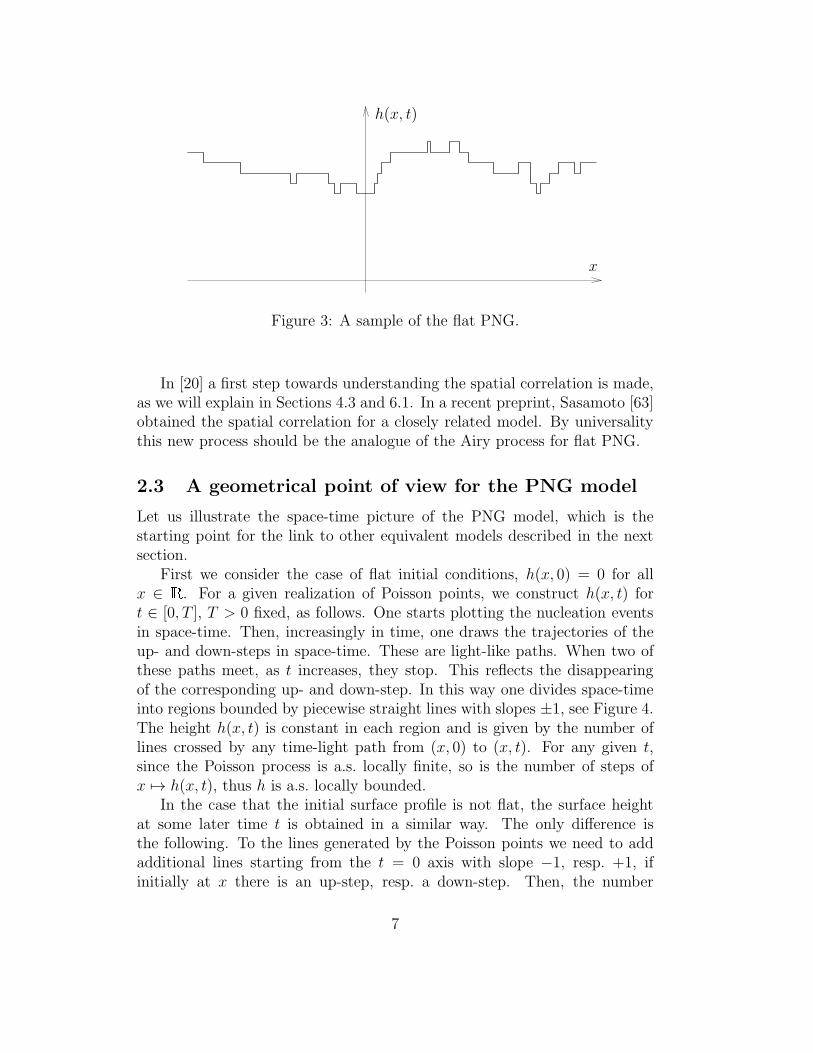
2.2 Flat PNG

A flat initial condition, h(x, 0) = 0 for x ∈ R, and constant density ofPoisson points in R×R+ (as before we choose = 2) generates the flat PNGgeometry, see Figure 3. Since no other constraint is imposed the surfaceheight h(x, t) is statistically translation-invariant, thus we focus on x = 0.

The fluctuations live on the same scale as for the PNG droplet, namelyt1/3. However, the limiting distribution is different as shown in [56], namely

limt→∞

P

(

h(0, t) ≤ 2t+ t1/32−2/3s)

= F1(s), (2.7)

with F1 the GOE Tracy-Widom distribution function [70]. This result fol-lows from a related problem on longest increasing subsequences [9]. Theconvergence is in distribution and for all moments as in (2.3).

6

PSfrag replacements

h(x, t)

x

Figure 3: A sample of the flat PNG.

In [20] a first step towards understanding the spatial correlation is made,as we will explain in Sections 4.3 and 6.1. In a recent preprint, Sasamoto [63]obtained the spatial correlation for a closely related model. By universalitythis new process should be the analogue of the Airy process for flat PNG.

2.3 A geometrical point of view for the PNG model

Let us illustrate the space-time picture of the PNG model, which is thestarting point for the link to other equivalent models described in the nextsection.

First we consider the case of flat initial conditions, h(x, 0) = 0 for allx ∈ R. For a given realization of Poisson points, we construct h(x, t) fort ∈ [0, T ], T > 0 fixed, as follows. One starts plotting the nucleation eventsin space-time. Then, increasingly in time, one draws the trajectories of theup- and down-steps in space-time. These are light-like paths. When two ofthese paths meet, as t increases, they stop. This reflects the disappearingof the corresponding up- and down-step. In this way one divides space-timeinto regions bounded by piecewise straight lines with slopes ±1, see Figure 4.The height h(x, t) is constant in each region and is given by the number oflines crossed by any time-light path from (x, 0) to (x, t). For any given t,since the Poisson process is a.s. locally finite, so is the number of steps ofx 7→ h(x, t), thus h is a.s. locally bounded.

In the case that the initial surface profile is not flat, the surface heightat some later time t is obtained in a similar way. The only difference isthe following. To the lines generated by the Poisson points we need to addadditional lines starting from the t = 0 axis with slope −1, resp. +1, ifinitially at x there is an up-step, resp. a down-step. Then, the number

7

PSfrag replacements

x

tt = T

h = 0

h = 1

h = 2 h = 3h = 3

Figure 4: Graphical construction generating the surface height from the nu-cleation events (Poisson points).

of lines crossed along any time-like paths from (x, 0) to (x, t) is the heightdifference h(x, t)− h(x, 0).

2.4 Other geometries studied for the PNG model

As explained above, the one-point distribution function of the surface heightfor both geometries, the PNG droplet and flat PNG, was obtained by iden-tifying the surface height with the length of a longest directed polymer. Thedirected polymer can be mapped to a longest increasing subsequence in arandom permutation (without/with involution), for which Baik and Rainshave obtained the asymptotics [9, 8] by using Riemann-Hilbert techniques.For the PNG droplet, the joint-distribution of the height profile is obtainedin [57] using a multilayer generalization of the PNG as will be explainedin Section 4. The multilayer technique has been motivated by the work ofJohansson on the Aztec diamond [38, 40].

Sasamoto and Imamura studied the (discrete) half-droplet PNG geome-try, which consists in allowing nucleations only in the region x ∈ [0, t] [33].They prove that the rescaled height is GUE distributed away from x = 0 andthat there is a transition to GSE at x = 0. If extra nucleations are added atthe origin with intensity γ ≥ 0, the distribution above x = 0 has a transitionat γ = 1. For γ < 1 it is still GSE, for γ = 1 it is GOE distributed, andfor γ > 1 the fluctuations become Gaussian, because the contribution of thenucleations at the origin dominates. The asymptotic one-point distributionsat the origin follow from [9, 8], too.

A modification of the PNG droplet consists in adding sources at bothextremities of the droplet. Extra nucleations with fixed line density α+ and

8

α− are independently added along the boundary of the forward light cone ofthe origin, i.e., in (x, t) such that |x| = t. This model was used in [56] todescribe stationary PNG growth. Baik and Rains [7] obtained detailed resultsfor the asymptotic distributions which we describe briefly. For α± small, theeffects coming from the edges are small and the fluctuations are still GUEdistributed. On the other hand, if α+ > 1 or α− > 1, the boundary effects aredominant and the fluctuations become Gaussian. The cases where α+ = 1and/or α− = 1 are also studied and other statistics arise. Of particularinterest is when α+α− = 1 for 1 − α± = O(t−1/3), in which case the PNGgrowth is stationary and has a flat limit shape. Stationary PNG togetherwith flat PNG and PNG droplet are the three most interesting situations inthe context of surface growth.

Johansson in [36] pointed out the connection between random matricesand the shape fluctuations in a discrete model of directed polymers, equiva-lent to the discrete PNG model. A class of corner growth models in discretespace-time (similar to the PNG droplet) is analyzed in [30, 45]. The discreteversions of the different geometries for the PNG model discussed above arestudied in a series of papers [39, 33, 34, 35].

3 Equivalent models

In this section we discuss the mapping between models which are equivalentto the PNG model. We start explaining the directed polymers on Poissonpoints. The link to the PNG was used in [56] to obtain the first results on theheight fluctuations of the PNG model. Then we continue with the longest in-creasing subsequence problem, Young tableaux, a directed percolation model,the kink-antikink gas, and the Hammersley process.

3.1 Directed polymers on Poisson points

Let us define a partial ordering in R2, ≺, as follows. For y, z ∈ R2 we saythat y ≺ z if both coordinates of y are less or equal than those of z. Considera Poisson process with intensity 1 in R2. For a given realization of Poissonpoints, a directed polymer on Poisson points starting at (0, 0) and ending at(t, t) is a piecewise linear path γ connecting (0, 0) ≺ q1 ≺ . . . ≺ ql(γ) ≺ (t, t),where qi are Poisson points. The length l(γ) of the directed polymer γ is thenumber of Poisson points visited by γ. The basic observable of interest is themaximal length of the directed polymers,

L(t) = maxγ

l(γ). (3.1)

9

PSfrag replacements

xt

h(0, t)

(0, 0)

(t/√2, t/

√2)

Figure 5: Height and directed polymers for the droplet geometry

This is called point-to-point setting because both initial and final points arefixed.

A modification of the problem consists in considering the set of directedpolymers starting from (0, 0) and ending in the segment Ut = (y, z) ∈R

2+|y + z = 2t. This is called the point-to-line problem and the maximal

length is denoted by Lℓ(t).The link with the PNG model is apparent once we use the graphical point

of view explained in Section 2.3. In fact, for the PNG model, h(0, t) equalsthe number of lines (up- and down-steps trajectories) crossed by any light-like paths from (0, 0) to (0, t). In particular, one considers the paths whichcross them at the nucleation points and consist in straight segments betweenthese points. These are the directed polymers introduced above, up to a π/4rotation, see Figure 5. Because of the π/4 rotation, if the density of Poissonpoints in the PNG model and the directed polymer is the same, then h(0, t)equals L(t/

√2). To have a nicer formula, we set the density of Poisson points

to 2 for the PNG model and to 1 for the directed polymers. This impliesthat L(t) = h(0, t) of the PNG droplet and Lℓ(t) = h(0, t) of the flat PNG,both in distribution. Thus

limt→∞

P

(

L(t) ≤ 2t+ st1/3)

= F2(s), limt→∞

P

(

Lℓ(t) ≤ 2t+ s2−2/3t1/3)

= F1(s).

(3.2)

3.2 Longest increasing subsequences

Let SN denote the permutation group of the set 1, . . . , N. For each per-mutation σ ∈ SN , the sequence (σ(1), . . . , σ(N)) has an increasing subse-quence of length k, (σ(n1), . . . , σ(nk)), if σ(n1) < σ(n2) < . . . < σ(nk) and

10

n1 < n2 < . . . < nk. Denote by LN(σ) the length of the longest increasingsubsequences for the permutation σ. The problem of finding the asymptoticlaw of LN for a uniform distribution on SN is also called Ulam’s problem(1961) [75]. For a review around this problem, see [4]. Baik, Deift and Jo-hansson in the seminal paper [6] determined the fluctuation law of LN . Theyprove

limN→∞

P(LN ≤ 2√N + sN1/6) = F2(s), (3.3)

where F2 is the GUE Tracy-Widom distribution function. Compare (3.3)with (3.2), the role of t is taken over by

√N .

(3.3) is obtained using the Poissonized version of the problem, which isthe approach of the problem used by Hammersley [32]. Instead of fixingthe length of the permutations to N , one considers the set of permutationsS = ∪n≥0Sn and assigns the probability e−NkN/k! that a permutation isin Sk. Baik et al. first prove that (3.3) holds for this problem, and thenobtain the result via a de-Poissonization method, consisting in boundingfrom above and below the distribution of LN in terms of the Poissonized one.In a statistical physics language, the problem with fixed N corresponds tothe canonical ensemble, the one with Poisson distributed length to the grandcanonical ensemble, and the N → ∞ limit to the thermodynamical limit. Itis not surprising that the equivalence of ensembles holds for the observableLN . In fact, in the grand canonical ensemble the typical value of the numberof Poisson points is O(

√N) apart from N . Thus the correction to LN is of

order 1, which is vanishing small compared to N1/6 as N → ∞.The problem of the longest increasing subsequences in SN is equivalent

to the problem of finding the longest directed polymer from (0, 0) to (t, t)when N points are distributed uniformly in the square [0, t]2. The directedpolymers on Poisson points is the Poissonized version. In fact, consider aconfiguration of N points in the square [0, t]2. The length of the longestdirected polymer depends only on the order of their projections along bothaxis. Without changing this order we can put them on 1, . . . , N2. Thus toeach directed polymer there corresponds an increasing subsequence with thesame length. Hence the length of the longest directed polymer equals theone of the longest increasing subsequence. See Figure 6 for an example.

3.3 Young tableaux

Let λ = (λ1, λ2, . . . , λk) be a partition of the integer N , i.e., satisfyingλ1 ≥ λ2 ≥ . . . λk ≥ 1 and

∑ki=1 λi = N . λ is represented by a diagram with

k rows and with λi cells for row i, called Young diagram. A (standard)Young tableau of shape λ is a Young diagram, where the cells are filled

11

PSfrag replacements

i

σ(i)

1

1

2

2

3

3

4

4

5

5σ = (2, 3, 1, 5, 4)

P(σ) =

(

1 3 42 5

)

Q(σ) =

(

1 2 43 5

)

Figure 6: Longest increasing subsequences and directed polymers. (2, 3, 5)and (2, 3, 4) are the two longest increasing subsequences. The directed poly-mers of maximal length passes through the points labelled by (2, 3, 5) and(2, 3, 4).

by the numbers 1, 2, . . . , N , increasingly in each row and column. TheRobinson-Schensted correspondence is a bijection between permutationsσ ∈ SN and pairs of Young tableaux (P(σ),Q(σ)) with N cells and thesame shape. The algorithm leading to (P(σ),Q(σ)) is the following [64].

One starts with a pair of empty tableaux P and Q and fills thecells as follows:

P-tableau: for i from 1 to N , the number σ(i) is always placedvia row-bumping in the first row, i.e.,a) if σ(i) is larger than all numbers in the first row of theP-tableau, then append to the right of them,b) otherwise put it at the place of the smallest entry in the firstrow of P, which is larger than σ(i).In case b), the entry which was replaced is now placed viarow-bumping in the second row. If an entry is replaced in thesecond row, then it is placed via row-bumping in the third row,and so on.

Q-tableau: At each step in the generation of the P-tableau, itsshape is enlarged by one cell. For each i from 1 to N , put thenumber i at the position where a new cell appeared at step i inthe P-tableau.

12

i 1 2 3 4 5

σ(i) 2 3 1 5 4

P 2 2 3 1 32

1 3 52

1 3 42 5

Q 1 1 2 1 23

1 2 43

1 2 43 5

Table 1: Construction of the Young tableaux P(σ) and Q(σ) for the permu-tation σ = (2, 3, 1, 5, 4).

As an illustration in Table 1 we show the construction of the Young tableauxfor the permutation σ = (2, 3, 1, 5, 4) of Figure 6. By construction, theYoung tableaux P(σ) and Q(σ) have the same shape. Given a permutationσ ∈ SN , one places the points on N

2 with coordinates (i, σ(i)) and draws thelines as in Figure 6. Notice that the first row of P(σ) contains precisely thepositions of the horizontal lines at abscissa N +1/2, likewise the first row ofQ(σ) contains the positions of the vertical lines at ordinate N + 1/2. Thisproperty holds for all permutations which means that [4]

LN (σ) = λ1(σ). (3.4)

Consequently, a way to determine the asymptotic behavior of LN is byanalyzing the length of the first row of Young tableaux [76, 44]. The measureon the set of partitions of 1, . . . , N, YN , induced by the uniform measure onSN via the RS correspondence is the Plancherel measure PlN ; let dλ denotethe number of Young tableaux of shape λ, then

PlN (λ) =d2λ

∑

µ∈YNd2µ

, λ ∈ YN . (3.5)

The lengths λ2(σ), λ3(σ), . . . also have an interpretation in terms of di-rected polymers. This is discussed in Section 4.2.

3.4 A directed percolation model

Motivated by the discrete anisotropic directed polymers model of Rajeshand Dhar [60], one can reformulate the PNG model starting from a directedpolymer picture as follows. We take a stack of horizontal planesR2×N ⊂ R

3.Neighboring planes are connected by vertical bonds placed randomly. One

13

introduces the percolation cluster P ⊂ R

2×N as follows. In each plane thereis perfect directed percolation, i.e., if (x, y, k) ∈ P then (x′, y′, k)|x′ ≥ x, y′ ≥y ⊂ P . Percolation between adjacent planes occurs through the bonds, i.e.,if there is a bond from (x, y, k) to (x, y, k+1), then (x, y, k+1) ∈ P whenever(x, y, k) ∈ P .

If the position of the bonds between planes are given by independentPoisson processes of intensity 1, then the cluster spreading from the origin,(0, 0, 0), corresponds to the point-to-point directed polymer. The height ofthe cluster at (x, y) is the largest k such that (x, y, k) ∈ P . Thus the heightat (x, y) equals, in distribution, the length of the longest directed polymerfrom (0, 0) to (x, y). Similarly, the point-to-line directed polymer correspondsto the cluster spreading from the line (x, y, k)|x + y = 0, k = 0. Definethe time axis as (x, x)|x ∈ R+. Then the PNG dynamics is recovered byslicing the percolating cluster perpendicularly to the time axis.

The percolation cluster arises as the continuum limit of the discrete modelof Rajesh and Dhar [60]. It appears also in the limit of large alphabets for amodel of sequence aligning [46].

3.5 Interacting particle models

The kink-antikink gas

Bennet et al. [11] studied an idealized model for solitons in the sine-Gordonmodel. There are two types of solitons, called kinks and antikinks. Kinksmove to the left with velocity −1, antikinks to the right with velocity 1.The solitons are point-like and do not interact, with the exception that, if akink and an antikink collide, they annihilate each other. On the other hand,there is a constant uniform rate of production of kink-antikink pairs, whichimmediately move apart with unit speed. In [11] the stationary distributionof the kink-antikink gas is studied on a finite ring and in the thermodynamiclimit. From the description of the PNG model it is clear that the kinksand antikinks can be identified with the up- and down-steps of the PNGheight profile. Thus any result for the PNG model has a translation tostatements for the kink-antikink gas and vice versa, provided initial andboundary conditions match. For example, the height above the origin forflat PNG equals the number of kinks and antikinks that passed through theorigin (with vacuum as initial condition).

14

Hammersley process

In order to tackle the longest increasing subsequence problem, Hammers-ley [32] used a particle system to prove that limN→∞E(LN )/

√N exists, see

also [3, 65]. There is only one kind of particles on [0, T ], which sometimesjump to the left a certain distance, but otherwise are at rest. The positionx = T serves as particle reservoir and initially no particles are in [0, T ). If aparticle jumps, it jumps to the left to a position uniformly chosen in the in-terval between the particle and its left neighbor (or, for the left-most particle,the origin). The jump rate for each particle is proportional to the distance toits left neighbor. Particles do not cross under the dynamics. Moreover, thespace-time points where the particles land form a Poisson point process in[0, T )×R+ with uniform density. It is easy to see that for a given realizationof Poisson points, the space-time trajectories of the particles correspond, upto a π/4 rotation, to the light-like lines generated by the nucleations in thePNG model of Figure 5. The PNG with sources corresponds to the Ham-mersley process with sources and sinks [15].

4 Description of the PNG via line ensembles

4.1 Non-intersecting line ensembles

The surface height of the PNG model at time T , x 7→ h(x, T ), does notcontain anymore the information of the position of the Poisson points, be-cause whenever two steps collide, information is lost. Therefore the measureinduced by the Poisson process on the set of heights is not easy to describe.A way of recording the lost information is to extend the model to a multi-layer version. This is achieved using the Robinson-Schensted-Knuth (RSK)construction [77].

Instead of a single line x 7→ h(x, t) evolving in time according to thePNG dynamics, one considers a set of lines x 7→ hℓ(x, t)|ℓ ≤ 0, with theidentification h0 ≡ h. The initial condition is hℓ(x, 0) = ℓ, x ∈ R, ℓ ≤ 0.The deterministic dynamics is identical for all the lines. Only the stochasticpart differs as follows. The first line follows the PNG dynamics as explainedin Section 2. If at time t an up- and a down-step annihilate at position x,one records the information in the second line in the form of a nucleationevent at (x, t). This procedure is repeated recursively, that is, the nucleationevents in the line hℓ−1 correspond to the annihilation events in the line hℓ.

As for the single line, also for the multilayer version of the PNG modelthere is a geometric point of view. In space-time, when two light-like linesgenerated by the Poisson points meet, they become light-like lines for the

15

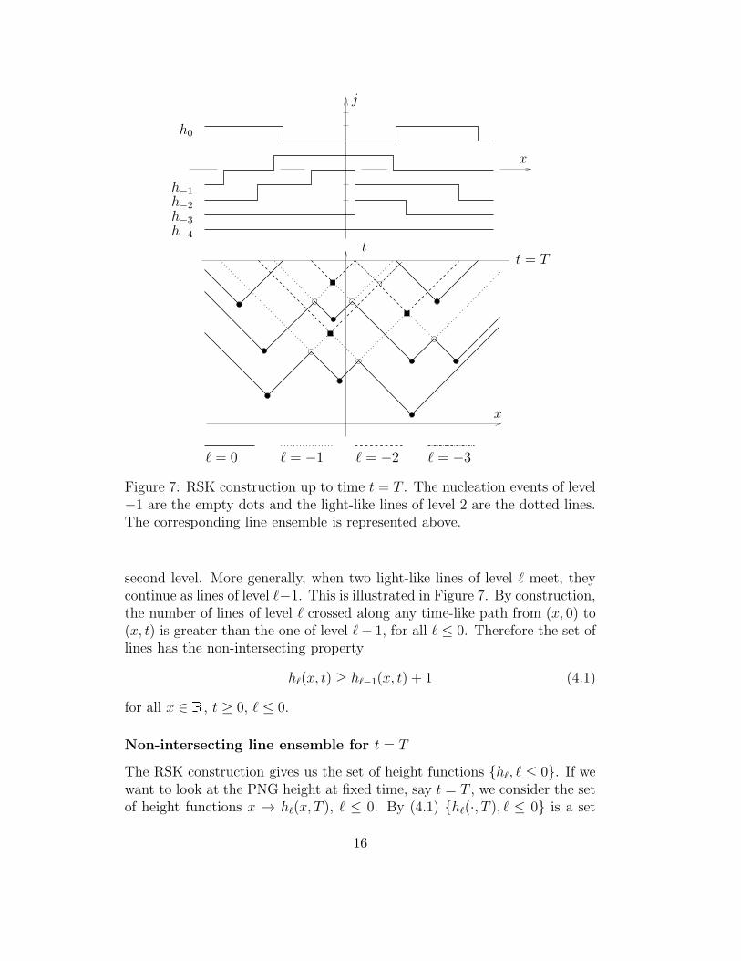
PSfrag replacements

x

x

tt = T

ℓ = 0 ℓ = −1 ℓ = −2 ℓ = −3

j

h0

h−1

h−2

h−3

h−4

Figure 7: RSK construction up to time t = T . The nucleation events of level−1 are the empty dots and the light-like lines of level 2 are the dotted lines.The corresponding line ensemble is represented above.

second level. More generally, when two light-like lines of level ℓ meet, theycontinue as lines of level ℓ−1. This is illustrated in Figure 7. By construction,the number of lines of level ℓ crossed along any time-like path from (x, 0) to(x, t) is greater than the one of level ℓ− 1, for all ℓ ≤ 0. Therefore the set oflines has the non-intersecting property

hℓ(x, t) ≥ hℓ−1(x, t) + 1 (4.1)

for all x ∈ R, t ≥ 0, ℓ ≤ 0.

Non-intersecting line ensemble for t = T

The RSK construction gives us the set of height functions hℓ, ℓ ≤ 0. If wewant to look at the PNG height at fixed time, say t = T , we consider the setof height functions x 7→ hℓ(x, T ), ℓ ≤ 0. By (4.1) hℓ(·, T ), ℓ ≤ 0 is a set

16

of non-intersecting lines with x 7→ h0(x, T ) the surface profile at time T , seeFigure 7.

Non-intersecting line ensemble for other space-time cuts

In some situations, as in the work on the flat PNG [20], it can be convenientto analyze a line ensemble which corresponds to another space-time cut.Consider a continuous and piecewise differentiable path γ : I → R × [0, T ],I ⊂ R an interval. Then the line ensemble corresponding to γ, denotedby Hℓ, ℓ ≤ 0, is given by Hℓ(s) = hℓ(γ(s)), s ∈ I, ℓ ≤ 0. It is a non-intersecting line ensemble because of (4.1).

4.2 Line ensembles and (real valued) Young tableaux

We now explain the connection between line ensembles and Young tableaux.The height of the PNG surface above x = 0 at time t depends only on thePoisson points in the backward light cone of (0, T ), i.e., on (0,T ) = (x, t) ∈R×R+ s.t. |x| ≤ T−t. Let us consider the two space-time cuts γ1, γ2 givenby

s 7→ γ1(s) = (T − s, s), s ∈ [0, T ],

s 7→ γ2(s) = (s− T, s), s ∈ [0, T ]. (4.2)

Denote by H(1)ℓ , ℓ ≤ 0, resp. H(2)

ℓ , ℓ ≤ 0, the line ensemble along γ1, resp.γ2. From these two line ensembles we construct a pair of Young tableaux(Y1, Y2) as follows. Let us start with Y1. Let 0 < s1 < s2 < . . . < T be the

positions of steps in the line ensemble H(1)ℓ , ℓ ≤ 0. Let ℓi denote the line

in which the step at si occurs. Then Yk has the entry i in row j if the step atsi happens in the line H

(1)1−j, i.e., if ℓi = 1− j. Y2 is obtained in the same way

with step positions along γ2. On the other hand we can define a permutationσ ∈ SN , with N the number of Poisson points in (0,T ), by recording therelative positions of the projections of the Poisson points along γ1 and γ2.More precisely, we set (y, z) = (t+x, t−x) and label the Poisson points suchthat zi ≤ zi+1. Then, σ is the permutation such that yσ(i) ≤ yσ(i+1). SeeFigure 8 for a simple example. At first glance surprisingly, we have

Y1 = P(σ), Y2 = Q(σ). (4.3)

But a closer inspection reveals that the multilayer PNG dynamics is just atranslation of the algorithm in Section 3.3. In particular, this implies that

H(1)ℓ (T ) = H

(2)ℓ (T ) = λ1−ℓ + ℓ (4.4)

17

PSfrag replacements

γ1γ2

H(2)0

H(2)1

H(1)0

H(1)1 σ = (2, 3, 1)

P(σ) =

(

1 32

)

Q(σ) =

(

1 23

)

Figure 8: Young tableaux and line ensembles.

where λ0, λ1, . . . are the length of the rows of the Young tableaux.For the PNG droplet studied in [57], the measure on the Young tableaux

is the Poissonized Plancherel measure. For flat PNG the measure induced bythe Poisson points can still be studied if we introduce the symmetric imagesof the Poisson points with respect to the t = 0 axis, see [20] for details.In [33] a version of the PNG droplet is studied where the Poisson points aresymmetric with respect to x = 0. These two symmetries correspond to twodifferent involutions on the corresponding permutations, denoted by and in [9].

Length of the rows of Young tableaux. Given the permutation σ asabove, the interpretation of λi(σ), i = 1, . . . , k, follows from a theorem ofGreene [31]. Let, for i ≤ k, ai(σ) be the length of the longest subsequence ofσ consisting of i disjoint increasing subsequences. Greene proves that

ai(σ) = λ1 + · · ·+ λi. (4.5)

In terms of directed polymers, ak is the maximal sum of the lengths of k non-intersecting directed polymers from (0, 0) to (t, t), where non-intersectingmeans without common Poisson points.

Real-valued Young tableaux. From a different point of view, the line en-sembles can be regarded as a generalization of Young tableaux for real valuedentries. Consider a configuration of Poisson points with N points in (0,T )

ordered as above. Then one can run the Robinson-Schensted algorithm withthe replacements,

i −→ zi, σ(i) −→ yi, (4.6)

for i = 1, . . . , N . In this way one obtains a pair of Young tableaux with yi, zias entries. This pair of real-valued Young tableaux contains exactly the same

18

information as the line ensembles (H(1)ℓ , H

(2)ℓ ). More precisely, yi (resp. zi) is

in row j of P (resp. Q) if there is a step in the line H(1)1−j at yi (resp. in the

line H(k)1−j at zi).

4.3 Point process associated with the line ensemble

Our goal is to analyze the surface height h(x, T ). Therefore it is natural toconsider the line ensemble for t = T , x 7→ hℓ(x, T ), ℓ ≤ 0. Let us definethe extended point process ηT on R× Z given by

ηT (x, j) =

1, if there is a line passing through (x, j),0, otherwise.

(4.7)

ηT is an extended point process in the sense that, for any fixed x ∈ R,ηT (x, ·) is a point process on Z [50]. One can interpret the lines as trajecto-ries of fermions in imaginary time (reflecting the non-intersecting condition)where the particles, thus the associated point process, evolve following agiven (stochastic) dynamics [57]. We now explain the structure of the pointprocess ηT and the edge scaling for the PNG droplet and flat PNG.

Point process for PNG droplet: determinantal

For the PNG droplet it is enough to consider the line ensemble for x ∈[−T, T ], since for x ≤ −T and x ≥ T the lines are straight with hℓ(±T ) = ℓ,ℓ ≤ 0. As shown in [57], the measure on the configurations is the uniformone. Using the transfer matrix method it is shown that ηT is an extendeddeterminantal point process, which means that the n-point correlation func-tions ρ(n)(x1, j1; . . . ; xn, jn) can be expressed as a n×n determinant. For thePNG droplet the kernel is the extended Bessel kernel BT (x1, j1; x2, j2), thus

ρ(n)(x1, j1; . . . ; xn, jn) = det(

BT (xk, jk; xl, jl))

1≤k,l≤n. (4.8)

To analyze the surface one defines the edge scaling of the point process,compare with (2.5), by

ηedgeT (τ, s) = T 1/3ηT (τT2/3, ⌊2T

√

1− τ 2T−2/3 + sT 1/3⌋). (4.9)

In the T → ∞ limit, this extended point process converges to the extendeddeterminantal point process on R×R with extended Airy kernel

A(τ2, s2; τ1, s1) =

∫ 0

−∞dλ eλ(τ2−τ1) Ai(s1 − λ) Ai(s2 − λ), for τ2 ≥ τ1,

−∫∞

0dλ eλ(τ2−τ1) Ai(s1 − λ) Ai(s2 − λ), for τ2 < τ1.

(4.10)

19

where Ai is the Airy function as given in [1]. In particular for τ1 = τ2 (4.10)is equal to

A(s2; s1) =Ai(s2) Ai

′(s1)− Ai′(s2) Ai(s1)

s2 − s1, (4.11)

the classical Airy kernel [69].Let hresc

T be the rescaled height as defined in (2.5). The joint-distributionof hresc

T at positions τ1, . . . , τn can be written as a Fredholm determinant andin the limit of large growth time T

limT→∞

P

(

n⋂

k=1

hrescT (τk) ≤ sk

)

= det(1− f 1/2Af 1/2)L2((τ1,...,τn)×R) (4.12)

with fj(s) = Θ(s − sj). In this way in [57] the convergence of hrescT to the

Airy process is determined in the sense of finite-dimensional distributions.

The Airy process

The Airy process is defined by its finite-dimensional distribution [57, 40].For given s1, . . . , sn ∈ R and τ1 < . . . < τn ∈ R, we define f on Λ =τ1, . . . , τn ×R by f(sj, x) = χ(sj ,∞)(x). Then

P(A(τ1) ≤ s1, . . . ,A(τn) ≤ sn) = det(1− f 1/2Af 1/2)L2(Λ,dnx)

with A the integral operator with extended Airy kernel.The Airy process A was first introduced in [57] in the context of the PNG

droplet. There it was shown that A(t) has a version which is almost surelycontinuous, stationary in t, and invariant under time-reversal. Its single timedistribution is given by the GUE Tracy-Widom distribution. In particular,for fixed t,

P(A(t) > y) ≃ e−y3/24/3 for y → ∞,

P(A(t) < y) ≃ e−|y|3/12 for y → −∞, (4.13)

Thus the Airy process is localized. Define the function g by

Var(A(t)−A(0)) = g(t). (4.14)

From [57] we know that g grows linearly for small t and that the Airy processhas long range correlations:

g(t) =

2t+O(t2) for |t| small,g(∞)− 2t−2 +O(t−4) for |t| large. (4.15)

with g(∞) = 1.6264 . . .. The coefficient 2 in front of t−2 is determinedin [2, 78]. The Airy process has been recently investigated and a set ofPDE’s [2] and ODE’s [72, 73] describing it are determined.

20

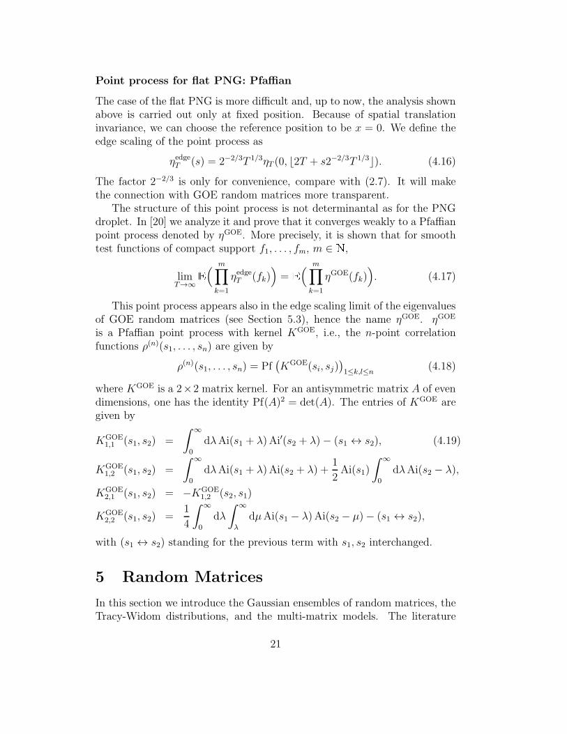
Point process for flat PNG: Pfaffian

The case of the flat PNG is more difficult and, up to now, the analysis shownabove is carried out only at fixed position. Because of spatial translationinvariance, we can choose the reference position to be x = 0. We define theedge scaling of the point process as

ηedgeT (s) = 2−2/3T 1/3ηT (0, ⌊2T + s2−2/3T 1/3⌋). (4.16)

The factor 2−2/3 is only for convenience, compare with (2.7). It will makethe connection with GOE random matrices more transparent.

The structure of this point process is not determinantal as for the PNGdroplet. In [20] we analyze it and prove that it converges weakly to a Pfaffianpoint process denoted by ηGOE. More precisely, it is shown that for smoothtest functions of compact support f1, . . . , fm, m ∈ N,

limT→∞

E

(

m∏

k=1

ηedgeT (fk))

= E(

m∏

k=1

ηGOE(fk))

. (4.17)

This point process appears also in the edge scaling limit of the eigenvaluesof GOE random matrices (see Section 5.3), hence the name ηGOE. ηGOE

is a Pfaffian point process with kernel KGOE, i.e., the n-point correlationfunctions ρ(n)(s1, . . . , sn) are given by

ρ(n)(s1, . . . , sn) = Pf(

KGOE(si, sj))

1≤k,l≤n(4.18)

where KGOE is a 2×2 matrix kernel. For an antisymmetric matrix A of evendimensions, one has the identity Pf(A)2 = det(A). The entries of KGOE aregiven by

KGOE1,1 (s1, s2) =

∫ ∞

0

dλAi(s1 + λ) Ai′(s2 + λ)− (s1 ↔ s2), (4.19)

KGOE1,2 (s1, s2) =

∫ ∞

0

dλAi(s1 + λ) Ai(s2 + λ) +1

2Ai(s1)

∫ ∞

0

dλAi(s2 − λ),

KGOE2,1 (s1, s2) = −KGOE

1,2 (s2, s1)

KGOE2,2 (s1, s2) =

1

4

∫ ∞

0

dλ

∫ ∞

λ

dµAi(s1 − λ) Ai(s2 − µ)− (s1 ↔ s2),

with (s1 ↔ s2) standing for the previous term with s1, s2 interchanged.

5 Random Matrices

In this section we introduce the Gaussian ensembles of random matrices, theTracy-Widom distributions, and the multi-matrix models. The literature

21

on random matrix is large, the standard reference book is [47], see also thereview [53].

5.1 Gaussian ensembles of random matrices

Let us define the two random matrix ensembles which are linked to the PNGdroplet and the flat PNG.

Gaussian unitary ensemble (GUE)

One defines a Gaussian measure on the set Ω of N × N complex Hermitianmatrices which is invariant under unitary transformations. Let H ∈ Ω, then

P(H)dH =1

Zexp(−Tr(H2)/2N)dH (5.1)

where dH =∏N

i=1 dHi,i

∏

1≤i<j≤N dRe(Hi,j)dIm(Hi,j) is the product measureon the independent coefficients of N . Here and below Z stands for the propernormalization constant. The scaling factor 1/2N in (5.1) is chosen in orderto simplify the comparison with the results on the PNG.

One interesting quantity of random matrices is the distribution of theeigenvalues λ1, . . . , λN , which is obtained by integrating over the unitarygroup. The result is

P2,N(λ1, . . . , λN)dλ1 · · ·dλN =1

Z|∆N(λ)|2

N∏

j=1

e−λ2

j/2Ndλj , (5.2)

with ∆N(λ) the Vandermonde determinant

∆N (λ) = det(λj−1i )Ni,j=1 =

∏

1≤i<j≤N

(λj − λi). (5.3)

Gaussian orthogonal ensemble (GOE)

In this case the matrices are real symmetric and the measure is invariantunder orthogonal transformations. The probability distribution takes thesame form as in (5.1), with the reference measure dH =

∏

1≤i≤j≤N dHi,j.The integration over the orthogonal group leads to the distribution of theeigenvalues λ1, . . . , λN

P1,N(λ1, . . . , λN)dλ1 · · ·dλN =1

Z|∆N(λ)|

N∏

j=1

e−λ2

j/2Ndλj . (5.4)

22

5.2 Edge scaling, Tracy-Widom distributions

One can focus on the largest eigenvalue’s distribution when the size of thematrices N is large. The largest eigenvalue, λmax, takes value close to 2N andits fluctuations are of order N1/3 [48, 27, 69]. Tracy and Widom determinedthe scaling function of λmax with the following result [69, 70], see also theirreview paper [71]. Let Fβ,N(t) = Pβ,N(λmax ≤ t), then Fβ(s) defined by

Fβ(s) = limN→∞

Fβ,N

(

2N + sN1/3)

(5.5)

exists for β = 1, 2. F1 and F2 are called the GOE and GUE Tracy-Widomdistribution respectively. More precisely,

F2(s) = exp(

−∫ ∞

s

(x−s)q2(x)dx)

, F1(s) = exp(

−1

2

∫ ∞

s

q(x)dx)

F2(s)1/2

(5.6)where q is the unique solution of the Painleve II equation q′′ = sq + 2q3

satisfying the asymptotic condition q(s) ∼ Ai(s) for s → ∞.

5.3 Eigenvalues’ point process and its edge scaling

We now define the point process of the eigenvalues λ1, . . . , λN .

GUE point process: determinantal

We denote by ζGUEN the point process onR of the GUE eigenvalues λ1, . . . , λN ,

i.e.,

ζGUEN (λ) =

N∑

j=1

δ(λ− λj), λ ∈ R, (5.7)

with the abuse of notation δ(λ − λj) for the Dirac measure δλi. ζGUE

N is adeterminantal point process, see for example Chapter 5 of [47], with kernelgiven by the Hermite kernel

KHN (x, y) =

pN(x)pN−1(y)− pN−1(x)pN(y)

x− ye−(x2+y2)/4N , (5.8)

where pk(x) = (2πN)−1/4(2kk!)−1/2pHk (x/√2N) with the (standard) Hermite

polynomials pHk (x) = ex2 dk

dxk e−x2

.The edge scaling of the point process ζGUE

N corresponding to (5.5) is

ηGUEN (ξ) = N1/3ζGUE

N (2N + ξN1/3). (5.9)

23

The limit point processlim

N→∞ηGUEN = ηGUE (5.10)

is well defined. It is the determinantal point process with Airy kernel (4.11).The GUE Tracy-Widom distribution F2(s) can also be written as a Fredholmdeterminant

F2(s) = det(1−A)L2((s,∞),dx) (5.11)

with A the integral operator with Airy kernel. For more information ondeterminantal point processes, see for example [66].

GOE point process: Pfaffian

In the same way as for GUE we define the point process of the GOE eigen-values ζGOE

N . For even N , ζGOEN is a Pfaffian point process, see for example

Chapter 6 of [47]. For more recent developments on Pfaffian point processessee [59, 67]. The edge rescaled point process is then given by

ηGOEN (ξ) = N1/3ζGOE

N (2N + ξN1/3). (5.12)

In the N → ∞ limit, the point process ηGOEN converges [70] to the point pro-

cess ηGOE which has correlation functions given by (4.18). One consequenceis that the distribution of the largest eigenvalue can be written as a FredholmPfaffian (see Chapter 8 of [59]) or Fredholm determinant on the measurablespace ((s,∞), dx)

F1(s) = Pf(J −KGOE) =√

det(1+ JKGOE) (5.13)

with J(x, y) = δx,y

(

0 1−1 0

)

. An interpretation of the Fredholm determi-

nant as the one on the operator with integral kernel KGOE needs some careas pointed out by Tracy and Widom in [74], where they actually prove thatthe finite-N Fredholm determinant converges to F1(s).

The GOE kernel being a 2 × 2 matrix is not uniquely defined. In factusing Pf(X tKX) = det(X) Pf(K) [68] one obtains a family of kernels Kleading to the same correlation functions. For example, the kernels reportedin [28, 33] differ slightly from (4.19), but they are equivalent since they yieldthe same point process.

Very recently a new formula for the GOE Tracy-Widom distribution F1

was established. Let B(s) be the operator with kernel B(s)(x, y) = Ai(x +y + s). It then holds

F1(s) = det(1−B(s)) (5.14)

where the Fredholm determinant is on L2(R+). This is proven in [25] startingfrom the work on the flat KPZ growth [63].

24

5.4 Multimatrix model: Dyson’s Brownian motion

Dyson [17] noticed that the distribution of eigenvalues (5.2) and (5.4) isidentical to the equilibrium probability distribution of the positions of Npoint charges, free to move in R under the forces deriving from the potentialU at inverse temperature β, with

U(x1, . . . , xN) = −∑

1≤i<j≤N

ln |xi − xj |+1

2Nβ

N∑

i=1

x2i . (5.15)

In the attempt to interpret the Coulomb gas as a dynamical system Dysonconsidered the positions of the particles in Brownian motion subjected tothe interaction forces −∇U and a frictional force f (which fixes the rateof diffusion, or equivalently, the time scale). He showed that in terms ofrandom matrices, this is equivalent to the evolution of the eigenvalues whenthe independent coefficients of the matrix H = H(t) evolve as independentOrnstein-Uhlenbeck processes given by

P (H(t) = H|H(0) = H0)dH =1

Zexp

(

−Tr(H − qH0)2

2N(1− q2)

)

dH (5.16)

with q = exp(−t/2N). The evolution of the eigenvalues satisfies the set ofstochastic differential equation

dλj(t) =

(

− 1

2Nλj(t) +

β

2

N∑

i=1,i 6=j

1

λj(t)− λi(t)

)

dt+ dbj(t) , j = 1, ..., N,

(5.17)with bj(t), j = 1, ..., N a collection of N independent standard Brownianmotions. The parameter β is 1 for GOE and 2 for GUE. We refer to the sta-tionary process of (5.17) as Dyson’s Brownian motion (for the eigenvalues).Note that for β ≥ 1 the process is well defined because there is no crossingof the eigenvalues, as proved by Rogers and Shi [61].

5.5 GUE extended point process

The GUE eigenvalues λi(t), i = 1, . . . , N define an extended point processon R+ ×R,

ζGUEN (t, λ) =

N∑

j=1

δ(λ− λj(t)). (5.18)

25

It is a determinantal point process [18] with kernel given by the extendedHermite kernel1,

KHN (t2, λ2; t1, λ1) =

∑−1k=−N ek(t2−t1)/2Npk(λ1)pk(λ2)e

−(λ2

1+λ2

2)/4N , t2 ≥ t1,

−∑∞k=0 e

k(t2−t1)/2Npk(λ1)pk(λ2)e−(λ2

1+λ2

2)/4N , t2 < t1,

(5.19)where pk(x) = pHN+k(x/

√2N)(

√2πN2kk!)−1/2 and pHk (x) the standard Her-

mite polynomials.The GUE Dyson’s Brownian motion is stationary and the edge scaling is

the following. Let ti = 2τiN2/3, λi = 2N + siN

1/3, i = 1, 2. In the limit oflarge N , KH

N converges in the edge scaling limit to the extended Airy kernel

limN→∞

N1/3KHN(2τ2N

2/3, 2N+s2N1/3; 2τ1N

2/3, 2N+s1N1/3) = A(τ2, s2; τ1, s1).

(5.20)This convergence is uniform for s1, s2 ∈ [a,∞) for any fixed a ∈ R, see forexample Appendix A.7 of [21]. Moreover, since it has (super-)exponentialdecay for large s1, s2 → ∞, one deduces that the largest eigenvalue convergesto the Airy process in the sense of finite-dimensional distributions,

limN→∞

N−1/3(λmax(2τN2/3)− 2N) = A(τ). (5.21)

6 PNG model, Young tableaux, and random

matrices

6.1 PNG model

Although the PNG model and the random matrix ensembles describe systemscompletely different, we can associate some point process via the multilayerextension and the integration over the symmetry groups, respectively. Thepoint processes happen to have the same mathematical structure:

(a) determinantal point processes for PNG droplet and GUE random ma-trices,

(b) Pfaffian point processes for flat PNG and GOE random matrices.

Moreover we have seen that, in the appropriate scaling limit, they convergeto the same limit objects. Thus the distribution of the largest eigenvalue and

1According to [73] this was already described in a MSRI lecture (2002) by Kurt Jo-hansson. It can be derived for example using Theorem 1.7 of [39], details can be found forexample in Appendix A.6 of [21].

26

the height of the PNG at fixed position have the same fluctuations in theasymptotic limit.

One natural question is whether such a connection still exists at the levelof joint-distribution (extended point processes). The extended point processfor the PNG model is naturally defined from the line ensemble. As explainedin Section 5.4 one defines the so-called Dyson’s Brownian motion (multi-matrix ensembles) and associates to it an extended point process. For GUErandom matrices it turns out that the extended point process has, in thelimit of large matrix dimension N , the extended Airy kernel, the same as forthe PNG droplet. As a consequence, the (droplet) surface height and theevolution of the largest (GUE) eigenvalue are described by the same processin the asymptotic limit [22]: the Airy process.

For GOE random matrices the answer is not known. It is conjectured thatthe surface height of the flat PNG and the evolution of the largest (GOE)eigenvalue converge to the same limit process. The result of Ferrari [20] makesthis conjecture more plausible. In fact, we now know that, not only h(0, T )in the limit T → ∞ and properly rescaled is GOE Tracy-Widom distributed,but also that the complete point process ηT converges to the edge scalingof Dyson’s Brownian motion with β = 1 for fixed time. For β = 1 Dyson’sBrownian motion this structure has not been unraveled and the questionremains open. Very recently, Sasamoto [63] obtained a process in the contextof the totally asymmetric exclusion process, which, by universality, shoulddescribe also the surface height of the flat PNG.

From the point of view of multi-matrices, the difficulty is the fact thatthe Harish-Chandra/Itzykson-Zuber formula doesn’t have a particularly niceanalogue for symmetric matrices. From the point of view of the SDE (5.17)the problem lies in the different factor in front of the drift term, which seemsto make it impossible to regard the process as Doob transforms of N inde-pendent processes [43].

There are other models with the same mathematical structure and show-ing the same limit behaviour (and scaling functions): the 3D-Ising cor-ner [52, 24] and the Aztec diamond [38, 40] which are linked via dominotilings, the vicious random walks and the non-colliding Brownian particles,see for example [49, 42], and the totally asymmetric exclusion process [26, 63].Some of the problems presented above can be solved by using orthogonalpolynomials point of view instead of the more geometric line ensembles, seefor example the review [43]. In this context the relevant processes are theSchur process [52] and its Pfaffian analogue [34, 14].

27

6.2 Young tableaux

In Section 4.4 we described the connection between the length of the row ofthe Young tableaux and the point process of the multilayer PNG. Above weexplained the connection between the multilayer PNG and the eigenvaluesof random matrices. Putting the two arguments together it follows thatthere is a connection between Young tableaux and random matrices. Afterhaving seen that the length of the first row of Young tableaux under thePlancherel measure (3.5) and the largest eigenvalue have the same statisticsin the asymptotic limit, it was conjectured by Baik, Deift, and Johansson thatthe connection would extend to the top rows, respectively top eigenvalues.They proved it for the second row in [5] and the first proof for all top rowsis due to Okounkov [51]. Other proofs are in [37, 12]. In the work onflat PNG [20] the point process with symmetric images was studied, whichcorresponds to the involution for permutations. In this case, the measureon the Young tableaux becomes Pl

(1)N (λ) = dλ, λ ∈ Y

(1)N , Y

(1)N being the

restriction of YN to the Young tableaux with λi even for all i. From theproof for the flat PNG [20] it follows that the top rows of Y

(1)N and the top

eigenvalues of GOE have the same limit joint-statistics.We first learned of the connection between the Young tableaux and the

random matrix ensembles for the GOE and GSE random matrix ensemblesby Sasamoto [62], where he deduced the connection starting from the PNGhalf-droplet [33]. For the GOE case the restriction that all λi have to be evenis not required. This result is also obtained by Forrester, Nagao, and Rainsin [29] using an approach with orthogonal polynomials.

References

[1] M. Abramowitz and I.A. Stegun, Pocketbook of mathematical functions,Verlag Harri Deutsch, Thun-Frankfurt am Main, 1984.

[2] M. Adler and P. van Moerbeke, PDE’s for the joint distribution of theDyson, Airy and Sine processes, Ann. Probab. 33 (2005), 1326–1361.

[3] D.J. Aldous and P. Diaconis, Hammersley’s interacting particle processand longest increasing subsequences, Probab. Theory Relat. Fields 103(1995), 199–213.

[4] D.J. Aldous and P. Diaconis, Longest increasing subsequences: frompatience sorting to the Baik-Deift-Johansson theorem, Bull. Amer. Math.Soc. 36 (1999), 413–432.

28

[5] J. Baik, P. Deift, and K. Johansson, On the distribution of the length ofthe second row of a Young diagram under Plancherel measure, Geom.Funct. Anal. 10 (2000), 702–731.

[6] J. Baik, P.A. Deift, and K. Johansson, On the distribution of the lengthof the longest increasing subsequence of random permutations, J. Amer.Math. Soc. 12 (1999), 1119–1178.

[7] J. Baik and E.M. Rains, Limiting distributions for a polynuclear growthmodel with external sources, J. Stat. Phys. 100 (2000), 523–542.

[8] J. Baik and E.M. Rains, The asymptotics of monotone subsequences ofinvolutions, Duke Math. J. 109 (2001), 205–281.

[9] J. Baik and E.M. Rains, Symmetrized random permutations, RandomMatrix Models and Their Applications, vol. 40, Cambridge UniversityPress, 2001, pp. 1–19.

[10] A.L. Barabasi and H.E. Stanley, Fractal concepts in surface growth,Cambridge University Press, Cambridge, 1995.

[11] C. Bennett, M. Buttiker, R. Landauer, and H. Thomas, Kinematics ofthe forced and overdamped Sine-Gordon soliton gas, J. Stat. Phys. 24(1981), 419–442.

[12] A. Borodin, A. Okounkov, and G. Olshanski, On asymptotics ofPlancherel measures for symmetric groups, J. Amer. Math. Soc. 13(2000), 481–515.

[13] A. Borodin and G. Olshanski, Stochastic dynamics related to Plancherelmeasure, arXiv:math-ph/0402064 (2004).

[14] A. Borodin and E.M. Rains, Eynard-Mehta theorem, Schur process, andtheir Pfaffian analogs, arXiv:math-ph/0409059 (2004).

[15] E. Cator and P. Groeneboom, Hammersleys process with sources andsinks, To appear in Ann. Probab. (2005).

[16] D. Dhar, An exactly solved model for interfacial growth, Phase Transi-tions 9 (1987), 51.

[17] F.J. Dyson, A Brownian-motion model for the eigenvalues of a randommatrix, J. Math. Phys. 3 (1962), 1191–1198.

29

[18] B. Eynard and M.L. Mehta, Matrices couples in a chain. I. Eigenvaluescorrelations, J. Phys. A 31 (1998), 4449–4456.

[19] P.L. Ferrari, Java animation of the RSK dynamics,http://www-m5.ma.tum.de/pers/ferrari/homepage/animations/(2004).

[20] P.L. Ferrari, Polynuclear growth on a flat substrate and edge scaling ofGOE eigenvalues, Comm. Math. Phys. 252 (2004), 77–109.

[21] P.L. Ferrari, Shape fluctuations of crystal facets and surface growthin one dimension, Ph.D. thesis, Technische Universitat Munchen,http://tumb1.ub.tum.de/publ/diss/ma/2004/ferrari.html, 2004.

[22] P.L. Ferrari, M. Prahofer, and H. Spohn, Stochastic growth in one di-mension and Gaussian multi-matrix models, ICMP 2003, 2003.

[23] P.L. Ferrari, M. Prahofer, and H. Spohn, Fluctuations of an atomic ledgebordering a crystalline facet, Phys. Rev. E, Rapid Communications 69(2004), 035102(R).

[24] P.L. Ferrari and H. Spohn, Step fluctations for a faceted crystal, J. Stat.Phys. 113 (2003), 1–46.

[25] P.L. Ferrari and H. Spohn, A determinantal formula for the GOE Tracy-Widom distribution, J. Phys. A 38 (2005), L557–L561.

[26] P.L. Ferrari and H. Spohn, Scaling limit for the space-time covari-ance of the stationary totally asymmetric simple exclusion process,arXix:math-ph/0504041 (2005).

[27] P.J. Forrester, The spectrum edge of random matrix ensembles, NuclearPhys. B 402 (1993), 709–728.

[28] P.J. Forrester, T. Nagao, and G. Honner, Correlations for theorthogonal-unitary and symplectic-unitary transitions at the hard andsoft edges, Nuclear Phys. B 553 (1999), 601–643.

[29] P.J. Forrester, T. Nagao, and E.M. Rains, Correlation functions forrandom involutions, arXiv://math.CO/0503074 (2005).

[30] J. Gravner, C.A. Tracy, and H. Widom, Limit theorems for height fluc-tuations in a class of discrete space and time growth models, J. Stat.Phys. 102 (2001), 1085–1132.

30

[31] C. Greene, An extension of Schensted’s theorem, Adv. Math. 14 (1974),254–265.

[32] J.M. Hammersley, A few seedlings of research, Proc. Sixth BerkeleySymp. Math. Statist. and Probability (University of California Press,ed.), vol. 1, 1972, pp. 345–394.

[33] T. Imamura and T. Sasamoto, Fluctuations of a one-dimensionalpolynuclear growth model in a half space, J. Stat. Phys. 115 (2004),749–803.

[34] T. Imamura and T. Sasamoto, Fluctuations of the one-dimensionalpolynuclear growth model with external sources, Nucl. Phys. B 699(2004), 503–544.

[35] T. Imamura and T. Sasamoto, Polynuclear growth model, GOE2

and random matrix with deterministic source, arXiv:math-ph/0411057(2004).

[36] K. Johansson, Shape fluctuations and random matrices, Comm. Math.Phys. 209 (2000), 437–476.

[37] K. Johansson, Discrete orthogonal polynomial ensembles and thePlancherel measure, Annals of Math. 153 (2001), 259–296.

[38] K. Johansson, Non-intersecting paths, random tilings and random ma-trices, Probab. Theory Related Fields 123 (2002), 225–280.

[39] K. Johansson, Discrete polynuclear growth and determinantal processes,Comm. Math. Phys. 242 (2003), 277–329.

[40] K. Johansson, The arctic circle boundary and the Airy process, Ann.Probab. 33 (2005), 1–30.

[41] K. Kardar, G. Parisi, and Y.Z. Zhang, Dynamic scaling of growing in-terfaces, Phys. Rev. Lett. 56 (1986), 889–892.

[42] M. Katori, T. Nagao, and H. Tanemura, Infinite systems of non-collidingBrownian particles, to appear in: Adv. Stud. Pure Math. (2003).

[43] W. Konig, Orthogonal polynomial ensembles in probability theory,arXiv:math.PR/0403090 (2004).

[44] B.F. Logan and L.A. Shepp, A variational problem for random Youngtableaux, Adv. Math. 26 (1977), 206–222.

31

[45] S.N. Majumdar and S. Nechaev, Anisotropic ballistic deposition modelwith links to the Ulam problem and the Tracy-Widom distribution, Phys.Rev. E 69 (2004), 011103.

[46] S.N. Majumdar and S. Nechaev, Exact asymptotic results for a model ofsequence alignment, arXiv:q-bio.GN/0410012 (2004).

[47] M.L. Mehta, Random matrices, 3rd ed., Academic Press, San Diego,1991.

[48] G. Moore, Matrix models of 2D quantum gravity and isomonodromicdeformation, Prog. Theoret. Phys. Suppl. 102 (1990), 255–285.

[49] T. Nagao, M. Katori, and H. Tanemura, Dynamical correlations amongvicious random walkers, Phys. Lett. A 307 (2003), 29–33.

[50] J. Neveu, Processus ponctuels, Ecole d’ete de Saint Flour, Lecture Notesin Mathematics (Berlin), vol. 598, Springer-Verlag, 1976, pp. 249–445.

[51] A. Okounkov, Random matrices and random permutations, Int. Math.Res. Not. 20 (2000), 1043–1095.

[52] A. Okounkov and N. Reshetikhin, Correlation function of Schur processwith application to local geometry of a random 3-dimensional Youngdiagram, J. Amer. Math. Soc. 16 (2003), 581–603.

[53] L. Pastur, Random matrices as paradigm, Mathematical Physics 2000(Singapore), World Scientific, 2000, pp. 216–266.

[54] A. Pimpinelli and J. Villain, Physics of crystal growth, Cambridge Uni-versity Press, Cambridge, 1998.

[55] M. Prahofer, Stochastic surface growth, Ph.D. thesis, Ludwig-Maximilians-Universitat, Munchen,http://edoc.ub.uni-muenchen.de/archive/00001381, 2003.

[56] M. Prahofer and H. Spohn, Universal distributions for growth processesin 1 + 1 dimensions and random matrices, Phys. Rev. Lett. 84 (2000),4882–4885.

[57] M. Prahofer and H. Spohn, Scale invariance of the PNG droplet and theAiry process, J. Stat. Phys. 108 (2002), 1071–1106.

[58] M. Prahofer and H. Spohn, Exact scaling function for one-dimensionalstationary KPZ growth, J. Stat. Phys. 115 (2004), 255–279.

32

[59] E.M. Rains, Correlation functions for symmetrized increasing subse-quences, arXiv:math.CO/0006097 (2000).

[60] R. Rajesh and D. Dhar, An exactly solvable anisotropic directed percola-tion model in three dimensions, Phys. Rev. Lett. 81 (1998), 1646–1649.

[61] L.C.G. Roger and Z. Shi, Interacting Brownian particles and the Wignerlaw, Probab. Theory Related Fields 95 (1993), 555–570.

[62] T. Sasamoto, On the Baik-Deift-Johansson conjecture for orthogo-nal/symplectic case, Private communication, February (2004).

[63] T. Sasamoto, Spatial correlations of the 1D KPZ surface on a flat sub-strate, J. Phys. A 38 (2005), L549–L556.

[64] C. Schensted, Longest increasing and decreasing subsequences, Canad.J. Math. 16 (1961), 179–191.

[65] T. Seppalainen, Hydrodynamic scaling, convex duality and asymptoticshapes of growth models, Markov Process. Related Fields 4 (1998), 1–26.

[66] A. Soshnikov, Determinantal random point fields, Russian Math. Sur-veys 55 (2000), 923–976.

[67] A. Soshnikov, Janossy densities II. Pfaffian ensembles, J. Stat. Phys.113 (2003), 611–622.

[68] J.R. Stembridge, Nonintersecting paths, Pfaffians, and plane partitions,Adv. Math. 83 (1990), 96–131.

[69] C.A. Tracy and H. Widom, Level-spacing distributions and the Airykernel, Comm. Math. Phys. 159 (1994), 151–174.

[70] C.A. Tracy and H. Widom, On orthogonal and symplectic matrix en-sembles, Comm. Math. Phys. 177 (1996), 727–754.

[71] C.A. Tracy and H. Widom, Distribution functions for largest eigenvaluesand their applications, Proceedings of ICM 2002, vol. 3, 2002.

[72] C.A. Tracy and H. Widom, A system of differential equations for theAiry process, Elect. Comm. in Probab. 8 (2003), 93–98.

[73] C.A. Tracy and H. Widom, Differential equations for Dyson processes,Comm. Math. Phys. 252 (2004), 7–41.

33

[74] C.A. Tracy and H. Widom, Matrix kernel for the Gaussian orthogonaland symplectic ensembles, arXiv:math-ph/0405035 (2004).

[75] S.M. Ulam, Monte Carlo calculations in problems of mathematicalphysics, Modern Mathematics for the Engineer (E.F.Beckenbach, ed.),vol. II, McGraw-Hill, New York, Toronto, London, 1961, pp. 261–277.

[76] A.M. Vershik and S.V. Kerov, Asymptotics of Plancherel measure ofsymmetric group and the limiting form of Young tables, Sov. Math. Dolk.18 (1977), 527–531.

[77] G. Viennot, Une forme geometrique de la correspondence de Robinson-Schensted, Combinatoire et Representation du Groupe Symetrique, Lec-ture Notes in Mathematics, vol. 579, Springer-Verlag, Berlin, 1977,pp. 29–58.

[78] H. Widom, On asymptotic for the Airy process, J. Stat. Phys. 115(2004), 1129–1134.

34