on wave radar measurement - lancaster universityjonathan/rdr13.pdf · on wave radar measurement ......

Submitted to Ocean Dynamics – “13th wave” Special Ed.

On Wave Radar Measurement

Kevin Ewans1, Graham Feld2, and Philip Jonathan3

1Sarawak Shell Bhd, 50450 Kuala Lumpur, Malaysia.

[email protected]

Ph:+60128736970 2Shell Global Solutions, Aberdeen, UK. 3Shell Research Ltd, Chester, CH1 3SH, UK.

Abstract

The SAAB REX WaveRadar sensor is widely-used for platform-based wave measurement systems by

the offshore oil and gas industry. It offers in-situ surface elevation wave measurements at relatively

low operational costs. Furthermore, there is adequate flexibility in sampling rates, allowing in

principle sampling frequencies from 1 Hz to 10 Hz, but with an angular microwave beam width of 10

degrees and an implied ocean surface footprint in the order of metres, significant limitations on the

spatial and temporal resolution might be expected. Indeed there are reports that the accuracy of the

measurements from wave radars may not be as good as expected. We review the functionality of a

WaveRadar using numerical simulations to better understand how WaveRadar estimates compare

with known surface elevations. In addition, we review recent field measurements made with a

WaveRadar set at the maximum sampling frequency, in the light of the expected functionality and

the numerical simulations, and we include inter-comparisons between SAAB radars and buoy

measurements for locations in the North Sea.

Keywords

Wave measurement, Wave radar, Inter-comparison, Surface elevation, Wave spectra

1 Introduction Wave measurements are required for the operation of offshore oil and gas facilities, and wave

measurement devices that can be mounted on the offshore platform itself are attractive to

operators, because of their relatively low operational costs – they are easy to maintain and service

and do not require expensive ship time needed for deployment and recovery of wave buoys. In

addition, they offer the potential to measure absolute surface elevation, when mounted on a fixed

platform, providing the opportunity to investigate more fundamental aspects of the wave field.

Among the instrument types that have been used are wave staffs, lasers, and radars. A good

description of these can be found in Tucker and Pitt (2001). Lasers and radars offer the additional

advantage over devices such as wave staffs in that they are not in contact with the water and can

more easily be deployed and maintained. Grønlie (2004) gives a high level description of a number of

different radar techniques suitable for wave and surface current measurements and a number of

currently available commercial wave and current sensors that employ these techniques. Among

these is the SAAB WaveRadar, which Grønlie (2004) categorises as a direct sensor, as it involves

direct measurement of surface elevation. Indirect sensors are those, such as those based on ship

Philip.Jonathan

Typewritten Text

Revised version June 2014

Philip.Jonathan

Typewritten Text


navigation systems that involve derivation of wave information from images associated with Bragg

scattering at low grazing angles.

In a review of electromagnetic wave scattering theories, Valenzuela (1978) states that the

backscatter of electromagnetic waves from the ocean is specular near normal incidence; and away

from normal incidence the scattering is diffuse, being produced by the smaller scale roughness

characteristics. Accordingly, as the WaveRadar is mounted on a platform in a vertically downward-

looking orientation, the tangent-plane approximation, in which the surface fields may be

approximated by those that would correspond to a flat tangent plane existing at each point on the

surface, is valid. In such cases the scattered fields may be obtained using the physical optics or

Kirchoff method, but (Valenzuela, 1978) cautions that an effective reflection coefficient should be

used, and notes that the mean-square ocean wave slope influences the scatter, and small-scale

roughness associated with spray and foam modify the reflection. In this respect, breaking waves will

also have an effect on the scattering (e.g. Donelan and Pierson, 1987). In addition to the effect on

scattering, spray and foam may introduce errors in measurement; Grønlie (2004) notes that lasers

may lock onto water spray and fog, and will be frequently be unable to track the sea surface, but

that microwave radars are less susceptible to this, due their much lower frequency of operation.

While there is an extensive literature on the performance of wave radars based on low grazing angle

measurements (e.g. Story et al., 2001), there are few publications on the performance of surface

elevation measuring radars. Mai and Zimmermann (2000) found two “comparatively cheap” radar

level sensors – Vegaplus 1, Vega and Kalesto, Ott did not perform in a wave-flume, but these were

units specifically set up for tank level measurements. In the WACSIS project (Barstow et al., 2002),

wave measurements from five platform-based wave sensors – a Vlissingen step gauge, a Baylor wave

staff, a Thorn laser, a SAAB radar, and a MAREX SO5 radar – were compared. The significant wave

heights from the sensors were in agreement to within 3%. The SAAB radar was found to produce

higher crests and surface elevation skewness compared to the other instruments, but it was located

separately on a different part of the platform, and it was concluded that real spatial features in the

wave field could have caused the differences. They also concluded that there was only circumstantial

evidence of elevated crests caused by spray effects, and in many cases it was possible that dispersive

and/or short-crested effects may have caused the differences between the instruments. In addition,

they identified a number of events for which there was a lot of spray present, but where the

different instruments measured more or less the same crest heights, suggesting that ordinary spray

was not being picked up by any of the instruments.

The SAAB WaveRadar is widely-used by the offshore oil and gas industry. Shell alone has 12 facilities

in the North Sea instrumented with REX WaveRadars and 10 in the South China Sea. These data

provided the vast majority of the platform-based wave data analysed as a part of the CresT JIP

project (Christou and Ewans, 2011). The WaveRadar can be set to sample continuously at

frequencies up to 10 Hz, apparently providing excellent temporal resolution for the study of wave

processes; but with a specified angular microwave beam width of 10 degrees and an implied ocean

surface footprint in the order of metres, significant limitations in the spatial resolution and

consequently the effective temporal resolution might be expected. Noreika et al. (2011) report an

inter-comparison between measurements made with a Datawell Directional Waverider buoy (DWR)

and a SAAB Rex WaveRadar off the Australian Northwest Shelf. The WaveRadar was mounted at an

elevation of 26 metres above the water surface on Woodside Energy Limited’s North Rankin A (NRA)


platform, 135 km north-northwest of Dampier, and the DWR was deployed 3km away in 125 metres

of water.

Data were compared from parallel measurements made over a two year period, covering a wide

range of conditions. The WaveRadar sea states were found to produce significant wave heights 4%

to 10% lower than the DWR, with the biggest departure occurring during tropical cyclone conditions.

At storm peak sea states, the WaveRadar significant wave heights were 16% less than those from the

DWR. However, the significant wave height calculated from the spectrum corresponding to wave

periods longer than nine seconds and wave periods were in good agreement. We present results in

this paper that do not show such a bias between wave buoy measurements and WaveRadar

measurements in the North Sea.

Nevertheless, the uncertainty of the effect of the resolution of the wave radar on the measurements

remains, and it was the objective of the work reported in this paper, to gain an understanding of

this. Accordingly, we review the functionality of a WaveRadar using numerical simulations, based on

theoretical considerations, to better understand how the radar estimates compare with known

surface elevation. In addition, we review recent field measurements made with a Rex WaveRadar set

at the maximum sampling frequency in the light of the expected functionality and the numerical

simulations, and we present comparisons between WaveRadars and Datawell wave buoys at several

locations in the North Sea.

A description of the WaveRadar is given in Section 2; the numerical simulations undertaken to assess

the functionality of the radar are presented in Sections 3 and 4; the field measurements are given in

Section 5; and conclusions are given in Section 6.

2 The WaveRadar The WaveRadar REX is now manufactured by Rosemount Tank Radar AB, Gothenburg, Sweden, and

is a derivative of their TankRadar system. (The company was SAAB until 2001 when it was bought by

Emerson, and the radar unit is now part of the Rosemount group within Emerson). The first

WaveRadar was a land-based TRL unit installed in the early 90s by Rijkwaterstaat in The Netherlands.

The first TRL/2 unit was installed in May 1993, and late in 1999 the first WaveRadar Rex was tested

at the Shell Cormorant Alpha platform. There are more than 500 WaveRadars installed worldwide,

most of which are WaveRadar Rex gauges.

The WaveRadar consists of a transmitter head housing the electronics and a 0.44 m diameter

parabolic dish antenna (Plate 1). It employs the Frequency Modulated Continuous Wave (FMCW)

method for determining the range to the target. The signal is a low power (< 0.5 mW) frequency

modulated 9.7 to 10.3 GHz (linear sweep) continuous microwave signal. Each measurement cycle

consists of a linearly-increasing frequency sweep, followed by a linearly-decreasing frequency sweep

– producing a triangular frequency modulation signal. The transmitted signal changes frequency

during the time taken for the reflected signal to return. The received signal reflected from the water

surface is mixed with the signal that is being transmitted at that moment, and the result is a signal

with a beat frequency proportional to the distance to the surface. Various processing of the mixed

signal is performed, including digital filtering, spectral analysis, and “peak picking”, to convert the

beat frequency to a distance. During the measurement cycle of 10.3 Hz, a number of measurements


are produced and an average distance recorded. The measurement cycle includes both an increasing

frequency sweep, followed by a decreasing frequency sweep, allowing Doppler shifts to be averaged

out.

The manufacturer specifications (RS Aqua, 2009) quote an accuracy: Range < 50 m = ±6 mm, Range

> 50 m = ±12 mm; Maximum deviation: Range < 50 m = ±1 mm; Clear downward view of the sea

surface within at least a 10 angle conical beam; Range 3 m to 65 m from the adaptor (the

measurement datum or origin). The manufacturer calibrates every WaveRadar REX in a special

calibration facility; and due to the design and construction of the electronic and microwave unit, the

WaveRadar REX calibration is extremely stable and periodic re-calibration is not required.

Details on the theoretical relationships for the signals of frequency-modulated radars and scattering

can be found in Axelsson (1978) and Axelsson (1987).

Plate 1: WaveRadar REX mounted on a South China Sea platform.

3 Simulations

3.1 Method

3.1.1 Surface Wave Simulations

A simple plane sinusoidal wave of frequency 0.2 Hz, long crested in one horizontal direction, was

simulated first, to build some understanding of the radar simulations with this simple case before

examining the irregular wave case. The amplitude of this sinusoid was set to 1 metre.

Then, a linear simulation of the ocean surface was employed, to provide a more realistic surface for

the radar simulations. The simulations were produced with a JONSWAP frequency spectrum, with a


peak frequency of 0.10 Hz, and a bimodal directional distribution (Ewans, 1998). The frequency

spectrum was defined with a resolution of 6.3 × 10-4 Hz, over the range 0 to 10 Hz. The resolution

and range was chosen to provide a time series of 32,768 points with a time step of 0.0485 s. The

directional resolution was 1 degree. A contour plot of the frequency-direction spectrum is given in

Figure 1. The units of the colour contours are dB re. 1 m2Hz

-1deg

-1.

Figure 1: JONSWAP-bimodal frequency direction spectrum. Colour scale in dB re. 1 m2Hz-1deg-1.

At each time step, the surface was generated over a 5 m square at a resolution of 0.01 m, to provide

spatial resolution for surface waves with frequencies up to 10 Hz.

This particular simulation is discussed in detail in Sections 4.2.1 and 4.2.2, but additional simulations

were undertaken for different sea state conditions for comparison and are described in Section

4.2.3. The additional simulations were performed for JONSWAP frequency spectra, with spectral

peak periods of 0.060 Hz and 0.25 Hz, and also for a representation of the measured sea state at the

St Joseph platform that is discussed in Section 5.1. The sea states represented by a JONSWAP

spectrum with spectral peak periods of 0.060 Hz and 0.25 Hz result in significant wave heights of

13.0 m and 0.72m respectively, providing comparative results for a relatively extreme and a

relatively mild sea state. The additional JONSWAP simulations were performed in accordance with

the method described above. The St Joseph platform sea state simulation was produced from a

frequency-direction spectrum that consisted of the sum of a JONSWAP frequency spectrum, with

spectral peak period of 0.20 Hz, with Ewans (1998) spreading, and the measured frequency

spectrum between 0.05 Hz and 0.19 Hz, together with the directional spreading specified by Ewans

(2002).

3.1.2 WaveRadar simulations

The simulation of the WaveRadar essentially follows the physical optics method and involves a

number of modelling steps – specification of the radar antenna pattern, determining the range to

many points on the sea surface at an instant of time, modelling the attenuation as a function of

range, modelling the reflection from the sea surface at each point, accumulation of the echoes from


all of the points, and performing analysis of the accumulat

to determine the range corresponding to the measured surface elevation.

A complete simulation of the WaveRadar functionality would involve duplicating the FMC

entailing modelling the FMCW signal

returned signal at a specific time, associated with the echo

The frequency sweep process during the incre

figure shows the radar signal sweep begin

frequency ��, at time ��, over an elapsed time of around 50

starts to decrease returning to ��, over the ensuing 50ms; this is not shown in the figure. The

parallelogram with the thick borders depicts the frequencies of the received signal from the ocean

surface echoes. The time delay betwee

frequency is very small, corresponding to the point on the ocean surface closest to radar. The last

return at the given frequency occurs a short time later, correspond

the ocean surface. The diagram is relevant for a surface wave field that is stationary in time.

At an instant of time, the received signal from all the echoes corresponds to frequencies defined by

a vertical slice through the parallelogram, as for example th

make the assumption that each frequency (corresponding to a given range to a surface point) is

unique and the phase of the echo can be ignored. Taking the example of Figure 2, at

are determined from the difference in the frequencies between

the Fourier transform of the received signal mixed with the emitted signal

signal power as a function of delta f. In practice,

transform provides estimates of the amplitude

a peak corresponding to a particular frequency difference or

Figure 2: Schematic of the FMCW transmission

frequency stage.

wave” Special Ed.

of the points, and performing analysis of the accumulated signal strength from all of the echoes

to determine the range corresponding to the measured surface elevation.

A complete simulation of the WaveRadar functionality would involve duplicating the FMC

entailing modelling the FMCW signal over its triangular sweep through one cycle, and gathering the

time, associated with the echoes from all the ocean surface grid points.

during the increasing frequency stage is depicted in Figure 2.

the radar signal sweep beginning at frequency ��, at time ��, and linearly increasing to

, over an elapsed time of around 50 ms. At time ��, the signal frequency

, over the ensuing 50ms; this is not shown in the figure. The


surface echoes. The time delay between the radar transmission and the first return at each


return at the given frequency occurs a short time later, corresponding to the most dist

e ocean surface. The diagram is relevant for a surface wave field that is stationary in time.


a vertical slice through the parallelogram, as for example that given at ��. For a random surface, we


unique and the phase of the echo can be ignored. Taking the example of Figure 2, at ��om the difference in the frequencies between �� and �� and ��. At any given time

the Fourier transform of the received signal mixed with the emitted signal is calculated

delta f. In practice, this is done over the 50 ms sweep. The Fourier

transform provides estimates of the amplitudes of each frequency difference component

a particular frequency difference or range of interest.

Figure 2: Schematic of the FMCW transmission and reflected signal frequencies over the increasing

signal strength from all of the echoes

A complete simulation of the WaveRadar functionality would involve duplicating the FMCW method,

gathering the

s from all the ocean surface grid points.

is depicted in Figure 2. The

, and linearly increasing to

, the signal frequency

, over the ensuing 50ms; this is not shown in the figure. The


n the radar transmission and the first return at each


to the most distant point on

e ocean surface. The diagram is relevant for a surface wave field that is stationary in time.


. For a random surface, we


�, the ranges

t any given time,

is calculated to determine

ms sweep. The Fourier

component, and it has

and reflected signal frequencies over the increasing


Our approach to the simulations is based on the assumption that the signal processing to convert

the frequency differences to ranges is done perfectly by the WaveRadar, to keep simulation times to

a manageable level, and also because the actual processing performed is proprietary and unknown.

Accordingly, we jump directly to what would be the output of the FMCW frequency analysis – the

reflected signal intensity (or gain) as a function of range, which is available directly from the

simulations.

Similarly, we minimise simulation times by treating the radar as a point source (located at the origin

of a rectangular Cartesian coordinate system with � positive upwards). This was considered justified,

due to the relatively small size of the antenna, and comparison of results from randomly choosing a

point on the surface of the radar as the source confirmed this.

Accordingly, it has been assumed that our signal is the summation of all the reflected signals from

the surface of the water at an instant of time. The ray diagram given in Figure 3 outlines the scenario

for a specific point, , on the surface.

The signal strength, �� , �� , ��, of the received echo from point, with vector location �� and

coordinates �� , �� , ��, on the ocean surface can then be expressed as:

�� , �� , �� = �� 2�� where �� is the antenna signal strength at the angle �� subtended by the point �� , �� , �� to the

downward vertical at the antenna location of �0,0,0�, where �� = � �� , �� is the

surface elevation, and �� is also a function of �� , �� , ��. � 2�� is the attenuation associated with path-loss over the range, �� = �� + �� + ��, and

� �� is the reflection coefficient corresponding to the radar signal reflection angle �� at

location , where �� is also a function of �� , �� , �� and equal to the angle between the

incoming ray from the radar and the local surface normal "� at �� , �� , ��. The total received signal at our instant of time is then simply the sum, ∑ �� , �� , �� .


Figure 3: Ray diagram for the point on the surface

The signal strength, ��, was obtained from the antenna beam pattern provided by RS-Aqua, the

suppliers of the Rosemount WaveRadar systems, and is given in Figure 4, with Swedish labelling.

Figure 4: WaveRadar antenna beam pattern.


We have used the Friis expression for the attenuation associated with propagation of the radar

signal, ��, given (in dB) by

�$%�� = −20log *4,2�- .

where - is the wavelength of the radar signal.

The backscatter from the ocean surface, which can range from specular to diffuse, is known to

depend on the mean-square slope of the surface (e.g. Liu et al, 2000), which can take on a wide

range of values, depending on the sea state and wind forcing. We investigate the backscatter effect

on the simulated radar surface elevation estimates for three diffuse reflector forms:

1. An ideal diffuse reflector, in which the intensity of reflection is the same for all reflection

angles. This type of reflectance is known as Lambertian, and we refer to is as “Lambertian” in

this paper.

2. A combined diffuse-specular reflector, defined by

�� = cos1��

The reflection in this case is symmetric about the reflected angle, but reduces (relatively

slowly) with increasing angle. We refer to this as “Diffuse” in this paper.

3. A combined diffuse-specular reflector, which is more specular than diffuse, defined by

�� = cos��

We refer to this as “Specular” in this paper.

The three reflection models are plotted in Figure 5. A gain of one signifies 100% reflection or a

perfect reflector. In our modelling, the Lambertian reflector is a perfect reflector for all angles, and

the Diffuse and Specular reflectors are perfect reflectors at the specular reflection angle. A more

physically realistic approach would be to turn these reflection forms into densities to better reflect

the scattering, but this would involve multiplying each by a constant, and the result would simply be

a change in the received signal gain, with the reflection gain from each point on the surface changed

by the same amount. As it is only the relative gain that is important, we chose to keep the reflection

forms simple.


Figure 5: Diffuse reflection models

With reference to Figure 3, the ray from the radar source, at point (0,0,0), to each surface point

must be determined. This ray then defines the range to the surface point, allowing the attenuation

associated with path loss to be determined, and the angle that the surface point subtends to the

vertical at �0,0,0�, allowing the appropriate attenuation antenna transmitter gain to be selected.

Accordingly, the position vector, ��, of the surface point, , relative to �0,0,0�, is simply given by

�� = �� , �� , ��, noting that �� = � �� , �� < 0. The set of all position vectors defines the surface

elevation � �� , ��. The magnitude of �� is the range to the surface point, and the angle that the surface point subtends

the vertical,�� at the source can be derived from the z-component, ��, of the direction cosines of

��, as

�� = cos3� �� ∙ 0,0, ��5��5

The diffuse-specular reflection component back toward the radar at point , is the reflection vector, 6� = −��, from which the reflection angle, ��, is determined from

�� = cos3� 6� ∙ "��7�

where "� is the vector normal to the surface at ��, and "� is calculated from the cross product of the

gradient of the surface defined by the position vectors, �, of all the surface points, as

"� = −�1,0, ∇�:� × 0,1, ∇�<� where ∇�: = =>

=: and ∇�< = =>=<


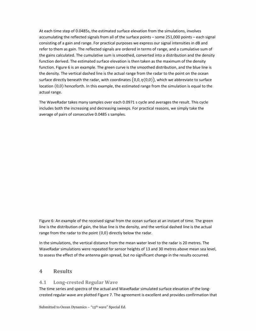
At each time step of 0.0485s, the estimated surface elevation from the simulations, involves

accumulating the reflected signals from all of the surface points

consisting of a gain and range. For practical purposes we express our signal intensities in

refer to them as gain. The reflected signals are ordered in terms of range, and a cumulative sum of

the gains calculated. The cumulative sum is smoothed, converted into a distribution and the density

function derived. The estimated surface elevation

function. Figure 6 is an example. The green curve is the smoothed distribution, and the blue line is

the density. The vertical dashed line is the actual

surface directly beneath the radar, with coordinates

location �0,0� henceforth. In this example, the estimated range from the simulation is equal to the

actual range.

The WaveRadar takes many samples over each

includes both the increasing and decreasing sweeps. For practical reasons, we simply take the

average of pairs of consecutive 0.0485 s samples.

Figure 6: An example of the received signal from the ocean surfac

line is the distribution of gain, the blue line is the density, and the vertical dashed line is the actual

range from the radar to the point �0In the simulations, the vertical distance from the

WaveRadar simulations were repeated for

to assess the effect of the antenna gain spread, but no

4 Results

4.1 Long-crested Regular Wave

The time series and spectra of the actual and WaveRadar simulated surface elevation of the long

crested regular wave are plotted Figure

wave” Special Ed.

he estimated surface elevation from the simulations, involves

accumulating the reflected signals from all of the surface points – some 251,000 points

For practical purposes we express our signal intensities in

The reflected signals are ordered in terms of range, and a cumulative sum of


function derived. The estimated surface elevation is then taken as the maximum of the density

is an example. The green curve is the smoothed distribution, and the blue line is

the density. The vertical dashed line is the actual range from the radar to the point on the ocean

ectly beneath the radar, with coordinates 0,0, ��0,0��, which we abbreviate to surface

. In this example, the estimated range from the simulation is equal to the

The WaveRadar takes many samples over each 0.0971 s cycle and averages the result. This cycle


average of pairs of consecutive 0.0485 s samples.

: An example of the received signal from the ocean surface at an instant of time. The green

line is the distribution of gain, the blue line is the density, and the vertical dashed line is the actual �0,0� directly below the radar.

In the simulations, the vertical distance from the mean water level to the radar is 20 metres. The

simulations were repeated for sensor heights of 13 and 30 metres above mean sea level,

to assess the effect of the antenna gain spread, but no significant change in the results occurred.

crested Regular Wave

actual and WaveRadar simulated surface elevation of the long

Figure 7. The agreement is excellent and provides confirmation that

he estimated surface elevation from the simulations, involves

some 251,000 points – each signal

For practical purposes we express our signal intensities in dB and

The reflected signals are ordered in terms of range, and a cumulative sum of


is then taken as the maximum of the density

is an example. The green curve is the smoothed distribution, and the blue line is

range from the radar to the point on the ocean

, which we abbreviate to surface

. In this example, the estimated range from the simulation is equal to the

the result. This cycle


e at an instant of time. The green

line is the distribution of gain, the blue line is the density, and the vertical dashed line is the actual

mean water level to the radar is 20 metres. The

30 metres above mean sea level,

change in the results occurred.

actual and WaveRadar simulated surface elevation of the long-

and provides confirmation that


the simulations are accurate. No discernible difference is apparent in the time series plot – Figure

7(a), while the spectral plot indicates minor deviation of the spectra from the simulations from the

surface elevation spectrum at high and low frequencies – Figure 7(b), but this occurs at more than

10 orders of magnitude below the spectral peak. The side lobes of the spectrum of the actual surface

are associated with the Blackman-Harris window used in the spectral analysis.

Figure 7: (a) The first 20 seconds of the time series of the surface elevation (directly beneath the

radar at the point (0,0)) and radar simulations of a simple plane wave with frequency 0.2 Hz and

amplitude of 1 m. (b) Spectra of the time series plotted in (a). In the plots, the surface elevation

signal is in black, the Lambertian signal is in blue, the Diffuse signal is green, and the Specular signal

is in red.

4.2 Random Linear Surface Elevation

The results of the random linear surface elevations are presented in this section. Comparisons

between the actual simulated surface elevations and the radar simulations for the JONSWAP

spectrum with a spectral peak frequency of 0.10 Hz are given in Section 4.2.1, while in Section 4.2.2

we review results for specific times in the time series, comparing and interpreting the results from

each of the surface reflection types, and providing some insight into the comparisons presented in

Section 4.2.1. We present the results of the additional simulations in Section 4.2.3, and we conclude

Section 4.2 with a general discussion of the results in Section 4.2.4.

4.2.1 Actual surface elevation and radar simulation comparisons

The surface elevation of the first 100 seconds of the simulated time series is presented in the left

plot of Figure 8. The discrepancies between the actual surface and the radar simulations are barely

discernible in the time series plot, but this is more apparent from the scatter plot of the data in

Figure 8 (right), which shows some spread in the simulations but virtually no overall bias. The scatter

is largest for the small elevations, which tend to be biased a little high. This is apparently due to

situations at times when the surface is elevated close to but not at the location (0,0), which

produces a larger gain at a shorter range in the simulations. It is interesting to note from the scatter

plot, that there is less scatter in the peaks and troughs of the time series, indicating the radar

estimates are closer to the actual values at those times. This is important for studying the individual

crest and heights in the time series.


Figure 8: Plots of the time series (left) and scatter plot (right) of actual and simulations of the surface

elevation for the three reflector types. In the plots, the surface elevation signal (time series plot

only) is in black, the Lambertian signal is in blue, the Diffuse signal is green, and the Specular signal is

in red.

Figure 9: Scatter plots of the zero-crossing crest and trough elevations for the three reflector types.

Figure 9 shows scatter plots of the crest and trough elevations for this time series, for the three

reflector types. Clearly there is some scatter in the radar estimates of the crests and troughs. There

is a small but discernible bias in the crests but not in the troughs. The bias in the crests is likely due

to cases where a local maximum in the crest occurs at a point close to (0,0) that produces a larger

gain and shorter range in the simulations. However, there is generally better agreement between

the actual and estimated values for the largest crest and troughs. It is also interesting to note the

difference between the number of crests and troughs, given near the top of each plot. The radar

estimates have more zero-crossing crests and troughs than in the actual time series, and the number

for each reflector is different. This is almost certainly due to an increased number of occurrences of

small crests and troughs that are introduced by the three reflection models corresponding to the

noise associated with the range estimation algorithm.


The spectra are given in Figure 10. The blue curve is the spectrum of the actual surface, and the

coloured are the radar spectra, for the three different reflector types, plotted on linear scales on the

left and log scales on the right. As for the plane wave results, there is no discernible difference

apparent in the linear plot, but the log plot shows increased levels in the radar spectrum at high and

low frequencies, with departures becoming apparent for frequencies below 0.06 Hz for all reflector

types and above 0.8 Hz for the Specular reflector type and above 1.0 Hz for the Lambertian and

Diffuse reflector types. The spectral parameters, which were calculated over the frequency range 0

to 5.15 Hz, are given in the left plot and also in Table 1. The significant wave heights are identical to

three significant figures, the radar first moment periods, T1, are biased up to 1% short, and the

second moment periods, T2, biased 4-9% short. The departures of the parameters T1 and T2 from

the simulations to those of the original surface elevations is solely due to the increased high

frequency spectral levels of the radar simulations that occurs above 0.8 Hz.

Figure 10: The spectra of the time series – linear left and log right. The blue curve is the spectrum of

the actual surface, and the green, red and cyan are radar spectra for the different reflection types.

4.2.2 Results at specific times

In this section we investigate the simulated radar signal to help understand the effects observed in

Section 4.2.1. We examine the signal at three instants in time – 1.36 s, 53.48 s, and 64.13 s after the

start of the record. The signal at these times are of interest for the following reasons: the signal at

1.36 s is a typical wave crest height, and should represent a common result; the signal at 52.48 s is

an example when the wave height is small and of short period may provide some insight into the

cause of the scatter that we observed for small elevations (Figure 8, right hand plot); and the signal

at 64.13 seconds after the start of the record corresponds to the large peak in the first 100 s of the

time series (Figure 8), and is of interest because lower scatter is seen in the larger peaks (Figure 8,

right hand plot). We shall also see later that these three times turn out to be interesting examples in

terms of the reflected signal gain – the first has a very clear maximum corresponding exactly to the

vertical range to surface; the second has a clear local maximum corresponding to the vertical range

to the surface, but the maximum gain corresponds to a point on the surface that has a smaller range

than the vertical to the sensor; while the third does not have a clear local maximum corresponding

to the vertical range to the surface, and like the second, the maximum gain corresponds to a point

on the surface that has a smaller range than the vertical to the sensor.

An example of the results at an instant of time is given in Figure 11. The figure shows results at the

simulation time 1.36 s, which is the first crest to occur in the time series. Plot (a) is the time series

plot of the first 100 s, with the time of interest, 1.36 s, indicated with a cross. Plots (b) through to (f)


are contour plots over a 5 m square of the surface centred at the vertical through the centre of the

radar dish – plot (b) is the surface elevation; plot (c) is the range from the dish origin in metres; and

plots (d) to (e) are plot of the received signal gain for the Lambertian, Diffuse and Specular surface

relection cases respectively. Plots (g) to (f) are plots of the gain-range distribution and density for the

Lambertian, Diffuse and Specular surface reflector case respectively; the vertical dashed line is the

estimated distance to the surface for each example. The contours show respective values at points

on the surface given by the x and y coordinates, with the point �0,0� marked with a cross. The units

of the surface elevation are given in z-coordinate metres (where the WaveRadar is at position �0,0,0�), the units of the gain are in dB and are negative, and the units of the ranges (absolute

distance from the WaveRadar to the point on the surface) is in metres.

Figure 11: Results at simulation time 1.36 s - (a) time series plot of first 100 s (the cross is at 1.36 s),

(b) contour plot of surface elevation in metres over 5 m square, (c) contour plot of range in metres

over 5m square, (d) contour plot of received signal gain in decibels for the Lambertian surface

relection case over 5m square, (e) contour plot of received signal gain in decibels for the Diffuse

surface relection case over 5m square, (f) contour plot of received signal gain in decibels for the

Specular surface relection case over 5m square, (g) gain-range distribution and density in decibels

for the Lambertian surface reflector case (vertical dashed line is the estimated distance to the

surface), (h) gain-range distribution and density in decibels for the Diffuse surface reflector case

(vertical dashed line is the estimated distance to the surface), and (i) gain-range distribution and

density in decibels for the Specular surface reflector case (vertical dashed line is the estimated

distance to the surface).


The surface elevation contour plot (Figure 11(b)) shows that the distance to the surface at the radar

source (0,0,0) is around 18.6 m. This can also be read from the range contour plot (Figure 11(c)) at

the point (0,0). The actual value of 18.62 m is plotted as the vertical dashed line on the gain-range

plots (g) to (e). The contour plots of the reflected signal gain (Figures 12(d), (e), and (f)) show that

the most intense signals are those that are reflected directly beneath the radar source, even though

the range (Figure 11(c)) is less to locations at grid points around (-0.6,-1). The Diffuse gain contour

plot (Figure 11(e)) is noisier than that for the Lambertian case (Figure 11(d)), and in turn, the

Specular gain contour plot (Figure 11(f)) is noisier than the Diffuse plot. Thus, the degree of noise in

the received signal pattern increases with increasing specularity, but, the characteristics of the

patterns remain consistent, with maximum gain occurring in the vicinity of the point (0,0).

Figure 12: Results at simulation time 52.48 s - (a) time series plot of first 100 s (the cross is at 52.48

s), (b) contour plot of surface elevation in metres over 5 m square, (c) contour plot of range in

metres over 5m square, (d) contour plot of received signal gain in decibels for the Lambertian

surface relection case over 5m square, (e) contour plot of received signal gain in decibels for the

Diffuse surface relection case over 5m square, (f) contour plot of received signal gain in decibels for

the Specular surface relection case over 5m square, (g) gain-range distribution and density in

decibels for the Lambertian surface reflector case (vertical dashed line is the estimated distance to

the surface), (h) gain-range distribution and density in decibels for the Diffuse surface reflector case





The combined effect of reflected signal gain and range, from accumulating the gain across the range

by combining the gain and range in the contour plots, are presented in Figures 12(g), (h), and (i). The

plots shows that most of the reflected signal intensity falls within a narrow range, and that the

maximum of each density curve, which is taken as the radar estimate is, in each case, very close to

the actual range (dashed line). This result is clearly a consequence of the narrow antenna beam

width of the WaveRadar, but the maximum of the gain-range plot can be expected to vary,

depending on the wave field at a given time, and we have indeed observed less accurate and more

accurate examples. Examples of less accurate cases are given below.

The next example is the wave field at 52.48 seconds after the start (see Figure 12), for a case when

the wave height is small and of short period. At this time, the actual range to the point (0,0)

corresponds to a local maximum in each of the gain-range plots (Figures 13(g), (h), and (i)). However,

in each case, the maximum in the gain-range plot is at a shorter range, approximately 0.1m shorter,

corresponding to a point on the surface nearby but at a higher point on the wave, which is receding

from the point (0,0). Otherwise, the gain contour plots and gain-range plots are qualitatively the

same, and also similar to those in Figure 11.

The inaccuracy in the measured range here is a direct consequence of the method of choosing the

peak in the gain-range plot - simply taking the maximum of the data was sufficient to provide an

accurate estimate, for the results at 1.36 s, but this approach introduces an error, for the results at

52.48 s. Nevertheless, it is clear that due to the narrowness of the gain-range density function, it is

not possible to get a grossly inaccurate result, irrespective of the method to pick the peaks, and this

is primarily due to the narrowness of the radar antenna beam pattern. However, as we shall see

later, this error introduces bias at the high frequencies.

Figure 13 gives the results for the wave field at 64.13 seconds after the start of the record. This

corresponds to the largest peak in the first 100 s of the time series. The surface elevation contour

plot (Figure 13(b)), shows a crest directly below the radar, but there is a more elevated local peak at

(0.5,0), near to (0,0), the point of interest. The local peak is closer to the radar and provides a slightly

more intense reflected signal. This is the maximum in the gain-range plots for all three reflector

types (Figures 14(g), (h), and (i)). As for the previous case, the error is in the order of 0.1 metres.


Figure 13: Results at simulation time 64.13 s - (a) time series plot of first 100 s (the cross is at 64.13

s), (b) contour plot of surface elevation in metres over 5 m square, (c) contour plot of range in

metres over 5m square, (d) contour plot of received signal gain in decibels for the Lambertian

surface relection case over 5m square, (e) contour plot of received signal gain in decibels for the

Diffuse surface relection case over 5m square, (f) contour plot of received signal gain in decibels for

the Specular surface relection case over 5m square, (g) gain-range distribution and density in

decibels for the Lambertian surface reflector case (vertical dashed line is the estimated distance to

the surface), (h) gain-range distribution and density in decibels for the Diffuse surface reflector case




4.2.3 Additional Simulations

The spectra derived from the additional simulations generally showed similar characteristics to those

described in Section 4.2.1, showing good agreement within the frequency band 0.060 Hz to 0.80 Hz

but elevated spectral levels outside that frequency band, by comparison with the surface elevation

signal. It was also noted that the elevated spectral levels have a larger effect on the overall

differences between the surface elevation simulation and the wave radar estimates when the sea

state is lower, as can be seen in the spectral parameters derived from the additional simulations,

given in Table 1. In the table, two values are given for each parameter – one derived over the

complete bandwidth 0 – 5.15 Hz, and the other derived over the reduced bandwidth 0.06 – 0.60 Hz

specified in parentheses in the table. The significant wave heights from the wave radar simulations

for the lowest sea state are still less than 3% different from the surface elevation signal, but the


second moment period is up to 22% shorter. The values associated with the three reflector types

agree to better than 1% with the original signal for the reduced bandwidth of 0.06 – 0.60 Hz.

Table 1: Spectral parameter values calculated over the bandwidth 0 – 5.15 Hz and 0.06 – 0.60 Hz in

parentheses.

Simulation Parameter Signal Lambertian Diffuse Specular

JONSWAP

Tp = 0.10 Hz

Hs (m) 4.98 (4.98) 4.98 (4.98) 4.98 (4.98) 4.98 (4.98)

T1 (s) 8.42 (8.45) 8.37 (8.44) 8.37 (8.44) 8.33 (8.44)

T2 (s) 8.01 (8.10) 7.65 (8.09) 7.64 (8.09) 7.32 (8.08)

JONSWAP

Tp = 0.060 Hz

Hs (m) 13.00 (10.17) 13.01 (10.17) 13.00 (10.17) 12.99 (10.16)

T1 (s) 13.72 (11.74) 13.69 (11.73) 13.69 (11.73) 13.68 (11.73)

T2 (s) 12.83 (11.17) 12.59 (11.16) 12.58 (11.16) 12.37 (11.15)

JONSWAP

Tp = 0.25 Hz

Hs (m) 0.72 (0.71) 0.74 (0.72) 0.74 (0.72) 0.74 (0.72)

T1 (s) 3.53 (3.70) 3.34 (3.67) 3.34 (3.65) 3.36 (3.68)

T2 (s) 3.35 (3.63) 2.69 (3.60) 2.69 (3.60) 2.60 (3.61)

St. Joseph

Hs (m) 2.63 (2.62) 2.64 (2.63) 2.64 (2.63) 2.64 (2.63)

T1 (s) 6.55 (6.60) 6.44 (6.58) 6.44 (6.58) 6.41 (6.58)

T2 (s) 6.20 (6.34) 5.65 (6.31) 5.63 (6.31) 5.38 (6.31)

4.2.4 Discussion

Overall, the simulations show that the radar measurements of the sea surface are excellent in the

vicinity of the spectral peak. At frequencies well below, and well above the spectral peak

(approximately five times the spectral peak in the example presented here), the simulations are

biased high, but as these are for elevations with spectral densities more than two orders of

magnitude less than the spectral peak, they have little practical consequence, on the wave spectrum

and the significant wave height, and their effect is relatively small on estimates of the crests and

troughs. Periods calculated from the moments of the spectra are biased short on account of the

elevated spectral levels of the simulations at high frequencies, but the degree of bias will depend on

upper frequency used to calculate the spectral moments – if this is constrained to 0.60 Hz, little bias

will occur.

The inaccuracies in the simulations result from the approach to peak fitting the gain-range density.

We have simply chosen to take the maximum of the density. This introduces error when there is a

more elevated section of water close to the point directly below the radar at (0,0). We suspect that

it may possible to develop a better peak picking algorithm, which would yield improved accuracies.

5 Field Measurements This section involves analysis of wave data measured with WaveRadars in the field. In Section 5.1,

we present a wave spectrum for measurements acquired on a platform in the South China Sea at the

maximum sampling rate of 10 Hz, and in Section 5.2 we present comparisons between

measurements made with a WaveRadar and a nearby wave buoy at several locations in the North

Sea.


5.1 10 Hz Sample Measurements

The 10 Hz data were recorded with a Rex WaveRadar mounted at 13 metres above mean sea level

on the St Joseph Platform offshore Sabah in Malaysia. The water depth at the St Joseph Platform is

94 metres.

On 10th

June, 2012, the WaveRadar was set to record at the maximum sampling rate of 10 Hz. The

variance density spectrum was computed for one hour of data, starting at 16:00 hours, at which

time a local wind-sea was active in the region, responding to a local wind of around 15 m/s. The

spectrum is plotted on log axes in Figure 14.

The main features of this spectrum are the well defined spectral peak, and the rapid fall off in

spectral level at frequencies below the spectral peak and above the spectral peak. Below the

spectral peak, the spectral levels plateau to levels some three orders of magnitude below that of the

spectral peak. Above the spectral peak, the spectral levels fall to levels nearly six orders of

magnitude below the spectral peak. Over the frequency range 0.2 Hz to 0.8 Hz (≈ 1.6�B to 6.6�B) the

spectral levels fall off with �3C.D, which is consistent with observations that typically fall between �3C and �31 (Babanin, 2010). Accordingly, these appear to be reasonable measurements of the

equilibrium range of the spectrum of wind waves. Above 0.8 Hz, the spectrum continues to roll off at

a steady rate of �3�.E, until 4 Hz (≈ 33�B), when the spectral levels “kick up” to the Nyquist

frequency of 5 Hz. The “kick up” is symptomatic of aliasing, but for frequencies below 4 Hz, there is

little to suspect the spectral levels are erroneous. This being the case, the WaveRadar appears to be

resolving signals at high frequency that are nearly six orders magnitude smaller than those at the

spectral peak. This is substantially better than achieved with the simulations described in Section

4.2, suggesting the WaveRadar performs better in practice than modelled in the work reported in

this paper. This observation must however be tempered by the absence of corroborating evidence of

a �3�.E high frequency tail (to the Authors’ knowledge); if one assumes that the �3�.E range is not

reliable, we might conclude that the WaveRadar is producing reliable results out to 0.80 Hz, which is

similar to that achieved in the simulations.


Figure 14: The wave spectrum for wave measurements at St Joseph Platform at 16:00 hrs on 10th

June, 2012 local time, derived from a record of one hour in length and a sampling frequency of 10

Hz.

5.2 Comparisons with Other Sensors

The WaveRadar measurements used for the inter-comparisons presented here were made on the

North Cormorant, Gannet, and Auk platforms, at elevations of 28.7 m, 22.5 m, and 24.3 m

respectively. Plan views and photographs of these are given in Figure 15. The location of the

WaveRadar on each platform is indicated with a green dot on the plan view of each. The North

Cormorant WaveRadar location might be expected to result in measurements that have interference

from the platform, for sea states with predominant directions from the north to east sector. In the

case of the Gannet and Auk platforms these sectors would be southwest to north and east to south

respectively.


North Cormorant

Gannet

Auk

Figure 15: Plan views of the three North Sea platforms, with the locations of the WaveRadar marked

by a green dot. The photograph of each platform (below the plan view in each case) provides some

indication of the amount of wave shielding that the platform might provide.

The wave buoy used for the comparisons at North Cormorant was located approximately seven

kilometres north-northeast of the platform, and that for Auk was located about four kilometres west

of the platform; but as there was no buoy located at the Gannet platform, the data from a wave

buoy located at the Anasuria site, some 15 km to the northwest, were used for comparison with the

Gannet platform WaveRadar measurements. The locations are given in Figure 16, and details on the

data used in the comparisons are given in Table 2.

It has not been possible to retrieve all the measurement details of the buoys, but we believe the

moorings were standard, as recommended by Datawell, and all the processing, including spectral

analysis and derivation of the wave spectral parameters, was performed on-board by Datawell

firmware.

Two versions of the SAAB radar were involved in the measurements. Recent measurements were

made with the SAAB Rex WaveRadar, and the earlier measurements were with the predecessor to

the Rex, which we refer to simply as the SAAB WaveRadar in this paper when distinguishing it from

the Rex but both are referred to as WaveRadars. The SAAB WaveRadar had a different processor to

the SAAB Rex WaveRadar, providing a 5.12 Hz digital output rather than a variable output of 2 to 10

Hz in the case of the Rex. The spectral analysis of the WaveRadar signals followed the Welch (1967)

method, with sampling frequencies of 2.0 Hz for the earlier data and 4.0 Hz for the later data, record

lengths of around 30 minutes, and spectral moments calculated over frequencies out to 0.60 Hz.

GANNET


Table 2 provides statistical details of the comparisons of the significant wave heights between the

WaveRadar and buoys. The median is given for the WaveRadar and buoy data sets separately, and

the bias, standard error, and rms difference between the WaveRadar and buoy data sets is given. In

addition, statistics are given for data sets stratified by the mean wave direction measured by the

directional buoys for each sea state. These statistics include the slope and offset of the linear

regression parameters and the mean ratio of the WaveRadar significant wave height to the buoy

significant wave height. This ratio provides an estimate of the overall relative level of the significant

wave heights for each direction.

Table 2: Measurement time series details

North Cormorant - Saab North Cormorant – Saab Rex Auk Saab Gannet – Saab Rex

WaveRadar Saab Saab Rex Saab Saab Rex

Elevation 28.7 m 28.7 m 24.3 m 22.5 m

Buoy Wavec Wavec Wavec Directional Waverider

Distance 7 km 7 km 4 km 15 km (Anasuria)

Period 05-Nov-1995 to 02-Sep-2002 21-May-2003 to 01-Jan-2004 26-Jan-1987 to 29-Jan-2003 17-Feb-2012 to 31-Aug-2013

No. data 44,656 8,649 74,926 23,781

No. years 6.8 0.6 16.0 1.5

Radar Hs median 2.40 m 1.90 m 1.70 m 1.47 m

Buoy Hs median 2.40 m 1.80 m 1.61 m 1.58 m

Bias (buoy - Radar) 0.04 m -0.12 m -0.03 m 0.12 m

Std (buoy v radar) 0.21 m 0.24 m 0.20 m 0.16 m

RMS Diff (buoy v radar) 0.22 m 0.27 m 0.20 m 0.20 m

All Data All Data All Data All Data

Exp

osu

re

Slop

e

Offse

t

Ra

tio

Exp

osu

re

Slop

e

Offse

t

Ra

tio

Exp

osu

re

Slop

e

Offse

t

Ra

tio

Exp

osu

re

Slop

e

Offse

t

Ra

tio

N 0.95 0.06 0.98 1.07 -0.04 1.05 clear 1.00 0.06 1.04 0.95 -0.01 0.94

NE 0.94 0.05 0.97 1.10 -0.11 1.02 clear 0.99 0.04 1.03 clear 0.94 -0.01 0.93

E 0.93 0.08 0.97 1.08 -0.08 1.02 0.98 0.05 1.02 clear 0.95 -0.01 0.95

SE clear 0.94 0.08 0.97 clear 1.12 -0.15 1.03 0.98 0.04 1.01 clear 0.95 -0.02 0.93

S clear 0.96 0.08 0.99 clear 1.10 -0.10 1.04 0.96 0.06 1.00 clear 0.94 -0.03 0.93

SW clear 0.98 0.07 1.01 clear 1.08 -0.04 1.05 clear 0.98 0.07 1.02 0.93 -0.02 0.92

W clear 0.99 0.04 1.01 clear 1.09 -0.04 1.06 clear 1.00 0.07 1.04 0.93 -0.02 0.94

NW clear 0.97 0.04 1.00 clear 1.07 -0.03 1.06 clear 0.99 0.09 1.05 0.94 0.00 0.94

Omni 0.97 0.05 0.99 1.08 -0.06 1.05 0.99 0.06 1.03 0.95 -0.02 0.93

Platform-induced Attenuation 0.98 0.99 0.97 1.00

Top 10% Top 10% Top 10% Top 10%

Exp

osu

re

Slo

pe

Offse

t

Ra

tio

Exp

osu

re

Slo

pe

Offse

t

Ra

tio

Exp

osu

re

Slo

pe

Offse

t

Ra

tio

Exp

osu

re

Slo

pe

Offse

t

Ra

tio

N 0.88 0.50 0.97 0.93 0.84 1.07 clear 0.91 0.46 1.03 0.88 0.27 0.95

NE 0.88 0.35 0.96 0.98 0.47 1.10 clear 0.95 0.18 1.01 clear 0.94 0.01 0.95

E 0.78 0.70 0.95 0.92 0.61 1.09 0.76 1.00 1.01 clear 0.90 0.35 0.96

SE clear 0.82 0.88 0.97 clear 0.97 0.66 1.12 0.80 0.88 1.01 clear 0.88 0.30 0.95

S clear 0.79 1.17 0.98 clear 1.05 0.22 1.09 0.82 0.65 0.98 clear 0.89 0.24 0.95

SW clear 0.85 1.00 1.00 clear 0.75 1.38 1.09 clear 0.84 0.69 1.01 0.85 0.29 0.93

W clear 0.88 0.71 1.01 clear 0.87 0.87 1.09 clear 0.87 0.72 1.03 0.92 0.16 0.96

NW clear 0.88 0.62 0.99 clear 1.05 0.15 1.08 clear 0.88 0.71 1.03 0.89 0.20 0.95

Omni 0.86 0.71 0.99 1.00 0.40 1.08 0.88 0.55 1.02 0.92 0.12 0.95

Platform-induced Attenuation 0.98 0.99 0.98 1.00

A measure of the effect of the platform shielding is given by the row in Table 2 labelled Platform-

induced Attenuation. This obtained by taking an average of the ratio values for all the data in the

sectors from which wave blockage might be expected and another average ratio for those sectors

from which waves are not expected to be blocked by the platform (labelled clear in Table 2) and

then taking the ratio, �G, of these two average ratios, expressed by the following equation.


�G = 17HIJ�K IJLK⁄N

OP�1QHIJ�R IJLRS

T

�P�U

where IJ�K and IJLK are respectively the observed WaveRadar and buoy significant wave heights for

the sectors from which wave blocking is expected, IJ�R and IJLR are those for the sectors from

which wave blocking is not expected (labelled clear in Table 2).

Figure 16: The locations of the wave measurements.

Figure 17 presents scatter plots of the significant wave height derived from measurements made at

the North Cormorant facility with a Datawell Wavec buoy and SAAB WaveRadar, and Figure 18

presents scatter plots for the significant wave height from the Wavec buoy and a SAAB Rex

WaveRadar. The scatter plots are stratified by the mean wave direction derived from the Wavec

buoy, and the result of a linear regression for each data set is given at the top of each plot and also

in Table 2.

North Cormorant

Anasuria

Gannet

Auk


Figure 17: Scatter plots of the significant wave height measured by a Datawell Wavec buoy and a

SAAB WaveRadar, at the North Cormorant platform, stratified by mean direction of the waves at the

Wavec buoy.

The plots in Figure 17 show the scatter between the significant wave height estimates, with some

quite large differences for specific sea states, but the significant wave height ratios given in Table 2

show that the WaveRadar and Wavec buoy significant wave heights agree on average to within 3%

for any particular direction and to within 1% for all directions overall, with the WaveRadar values

biased low by 0.04 m (Table 2) by comparison with the buoy values. The average ratios in Table 2 are

generally higher and close to one when the waves are from the West, the side of the platform where

the radar was installed and the side most likely to be least affected by the presence of the platform.

Accordingly, these measurements suggest virtually no difference between the significant wave

heights derived from the Wavec and WaveRadar when platform interference of the wave field is

expected to be small.

Remarkably, the comparison between the SAAB Rex WaveRadar and the Wavec (Figure 18 and Table

2) show the WaveRadar to be producing significant wave heights up to 6% higher on average than

those from the Wavec, although the trend with wave direction is less notable than observed in

Figure 17. We do not have an explanation for this result. It is our understanding that the only

difference between the installations associated with the data sets presented in Figures 17 and 18 is

the different WaveRadar types, which we would not expect to account for the differences in the

results. Nevertheless, the differences between the two sets of comparisons does appear to be due


to the specific set up of the system rather than anything related to the actual ability of the sensor to

measure the wave heights.


SAAB Rex WaveRadar, at the North Cormorant platform, stratified by mean direction of the waves at

the Wavec buoy.

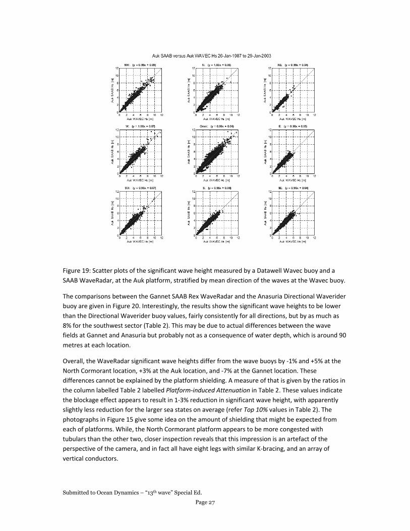
The results for the Auk platform are given in Figure 19. These results substantiate those observed in

Figure 17 – that the SAAB WaveRadar and Wavec significant wave heights are essentially the same

for wave directions not expected to result in significant platform interference with the wave field.



SAAB WaveRadar, at the Auk platform, stratified by mean direction of the waves at the Wavec buoy.

The comparisons between the Gannet SAAB Rex WaveRadar and the Anasuria Directional Waverider

buoy are given in Figure 20. Interestingly, the results show the significant wave heights to be lower

than the Directional Waverider buoy values, fairly consistently for all directions, but by as much as

8% for the southwest sector (Table 2). This may be due to actual differences between the wave

fields at Gannet and Anasuria but probably not as a consequence of water depth, which is around 90

metres at each location.

Overall, the WaveRadar significant wave heights differ from the wave buoys by -1% and +5% at the

North Cormorant location, +3% at the Auk location, and -7% at the Gannet location. These

differences cannot be explained by the platform shielding. A measure of that is given by the ratios in

the column labelled Table 2 labelled Platform-induced Attenuation in Table 2. These values indicate

the blockage effect appears to result in 1-3% reduction in significant wave height, with apparently

slightly less reduction for the larger sea states on average (refer Top 10% values in Table 2). The

photographs in Figure 15 give some idea on the amount of shielding that might be expected from

each of platforms. While, the North Cormorant platform appears to be more congested with

tubulars than the other two, closer inspection reveals that this impression is an artefact of the

perspective of the camera, and in fact all have eight legs with similar K-bracing, and an array of

vertical conductors.


To further put these results into perspective, it is useful to compare the differences in WaveRadar

and wave buoy significant wave heights with the results of the definitive wave sensor inter-

comparison test carried out in the WADIC project and reported by Allender et al. (1989). In that

project the significant wave heights measured with a number of sensors were compared against that

from a laser array at the Edda field in the North Sea. They found 2.5 – 5% discrepancy both positive

and negative to be common. Some were in the range 10-15%. It would appear therefore that our

comparisons are more or less consistent with the WADIC inter-comparisons.

Finally, it is important point to note that while the differences between the relationships from the

various comparison data sets remains to be explained, we do not observe a trend for the

relationships between the significant wave heights from the WaveRadars and buoys to change with

the value of the significant wave height. The results of regression analyses to the largest 10% of the

sea states for each direction are given in Table 2 (labelled Top 10%). The regression coefficients are

significantly different from those when all the data are utilised (labelled All Data in Table 2), with the

regression slopes of the Top 10% lower and the offset higher than the corresponding Top 10%

values. However, when the ratios of the WaveRadar to buoy significant wave height values are

compared between the Top 10% and the All Data data sets, they differ on average by ±5% at most.

Figure 20: Scatter plots of the significant wave height measured by a Datawell Directional Waverider

buoy at the Anasuria location and a SAAB WaveRadar, at the Gannet platform, stratified by mean

direction of the waves at the Directional Waverider buoy.


To conclude this section, we present results of comparing estimates of the spectral second moment

wave period, T2, from the WaveRadar and buoy for the four data sets. Averages of the ratio the

WaveRadar values to the buoy values are given in Table 3, for the blocked directional sectors

combined and for the clear directional sectors combined. The category referred to as Top 10% in the

table consists of the top 10% of the data with respect to the significant wave height. The agreement

between the WaveRadar and buoy T2 values is better than 7% and mostly better than 5%, with the

WaveRadar values being the larger in most cases.

We have been somewhat selective in the Auk data for the T2 comparisons. When all the data were

included for Auk, the scatter plot indicated more than one linear regression line would be needed to

explain the observations. This is believed to be due to some of the SAAB Rex WaveRider values

actually being zero-crossing periods from time-domain calculations rather than being estimates of

T2. We have excluded those values from the analysis. Nevertheless, uncertainty remains with the T2

comparisons for the Auk data set, and this may explain why these comparisons show a reverse trend

to those from the other three data sets.

The table also shows the ratios for the blocked sectors to be generally larger than for the clear

sectors for all cases, except for the Top 10% Auk SAAB data set. This suggests the platform blockage

may attenuate the higher frequency components in the wave field more than the lower frequency

components, as the value of T2 will be reduced if the high frequency spectral levels are decreased.

Table 3: Average values of the ratio of the WaveRadar T2 values to the buoy values.

North Cormorant - Saab North Cormorant – Saab Rex Auk Saab Gannet – Saab Rex

Platform Effect All Data All Data All Data All Data

Blocked 1.04 1.04 1.00 1.04

Clear 1.03 1.03 0.99 1.02

Platform Effect Top 10% Top 10% Top 10% Top 10%

Blocked 1.05 1.05 0.98 1.07

Clear 1.04 1.04 0.99 1.03

6 Conclusions Our simulations of WaveRadar measurements of a random linear surface wave field indicate that the

WaveRadar should faithfully follow the surface elevation at a point directly below the radar at

frequencies between 0.06 Hz and 0.6 Hz, and possibly out to 1.0 Hz. The main cause for the

departures in the simulated measurements outside that frequency band is due to the particular

method we have employed for processing the reflected radar signals, and especially the peak-picking

method. However, this has no effect on the significant wave height, but the elevated spectral levels

above 0.6 Hz can bias the spectral moment periods high by a few percent, if the calculation of the

spectral moments includes frequencies above 0.6 Hz.

Similarly, the departures in the simulated measurements outside that frequency band have no

appreciable effect on the calculated zero-crossing crests and troughs, though a small spread is seen

for small values of those parameters.


The field measurements made at a sampling frequency of 10 Hz indicate that the WaveRadar may

perform better than our simulations suggest, with the expected roll-off in spectral density continuing

to higher frequencies than the simulations, and the low-frequency plateau occurring an order of

magnitude lower relative to the spectral peak.

The comparisons of the significant wave height of WaveRadar measurements against Datawell wave

buoy measurements made in the North Sea generally show fairly good agreement and do not show

any trend with increasing significant wave height. Comparisons between the earlier WaveRadar units

and the Wavec buoy are in very good agreement for wave directions not expected to be affected by

the platform and small reductions in the WaveRadar values compared with the buoy values for

directions expected to be affected by the platform. Reduced significant wave heights due to

platform interference on the wave field are expected, but these appear to be just a few percent.

Comparisons of the Rex WaveRadars against the wave buoys show systematic differences in the

significant wave height in some cases. The differences are less than 8% and generally less than 5%,

and therefore more or less consistent with wave sensor inter-comparisons performed in the WADIC

experiment (Allender et al., 1989). Nevertheless, an explanation for these differences is desirable.

The differences cannot be explained by platform interference but appear to be more related to the

specific setup of the instrumentation, for which we currently do not have an explanation.

Accordingly, we acknowledge that further investigation of the field measurement setups is needed,

to explain the differences between the results of the various inter-comparisons, and we note

improvements in the WaveRadar “peak-picking” algorithm might lead to improved fidelity of the

simulations; but the results of this study support the conclusion that the WaveRadar provides good

measurements of the surface wave elevation, not only for supporting offshore operational activities

and engineering requirements but also for investigations into fundamental aspects of ocean surface

waves.

Acknowledgements The work described in this paper would not have been possible without the assistance of staff from

Emerson, who made time available to meet with one of us in Linköping for open discussion on the

functionality of the WaveRadar; and in particularly, we would like to thank Hakan Bertling and Jan

Westerling for providing additional information and responding to further questions following the

meeting.

References Allender, J., Audunson, T., Barstow, S. F., Bjerken, S., Krogstad, H. E., Steinbakke, P., Vartdal, L.,

Borgman, L. E., and C. Graham, 1989: The WADIC project: A comprehensive field evaluation of

directional wave instrumentation. Ocean Eng, 16, No. 5/6, 505-536.

Axelsson, S. R. J., 1978: Area target response of triangularly frequency-modulated continuous-wave

radars. IEEE Transactions on Aerospace and Electronic Systems. AES-14, 2, 266-277.


Axelsson, S. R. J., 1987: Characteristics of microwave backscattering from a ground surface with non-

isotropic roughness. 21st International Symposium on Remote Sensing of the Environment.

October 26-30, Ann arbour, Michigan.

Babanin, A.V., 2010: Wind input, nonlinear interactions and wave breaking at the spectrum tail of

wind-generated waves, transition from �3C to �31 behaviour. Ecological safety of coastal and

shelf zones and comprehensive use of shelf resources. Proceedings “To the 30th anniversary of

the oceanographic platform in Katsiveli”, Marine Hydrophysical Institute, Institute of

Geological Sciences, Odessa Branch of Institute of Biology of Southern Seas.- Sevastopol, 21,

173-187

Barstow, S. F., Krogstad, H. E., Lønseth, L., Mathisen, J. P. Mørk, G., and P. Schjølberg, 2002.

Intercomparison of sea state and zero-crossing parameters from the WACSIS field experiment

and interpretation using video evidence. Proceedings of OMAE’02 21st International

Conference on Offshore Mechanics and Artic Engineering, June 23-28, 2002, Oslo, Norway.

Christou, M., and K. C. Ewans, 2011: Examining a comprehensive data set containing thousands of

freak wave events. Part 1 – description of the data and quality control procedure. Proceedings

of OOAE2011 30th

International Conference on Ocean, Offshore and Arctic Engineering. 19 – 24

June, 2011, Rotterdam, The Netherlands.

Donelan, M. A., and W. J. Pierson, 1987. Radar scattering and equilibrium ranges in wind-generated

waves with application to scatterometry. J. Geophys. Res., 92, C5, 4971-5029.

Ewans, K. C., 1998: Observations of the directional spectrum of fetch-limited waves. Journal of

Physical Oceanography, 28, pp. 495–512.

Ewans, K. C., 2001: Directional spreading in ocean swell, Proceedings of Ocean Wave Measurement

and Analysis, San Francisco, 2001

Grønlie, Ø, 2004: Wave Radars A comparison of concepts and techniques. Hydro International, 8, No.

5, June.

Liu, Y., Su, M., Yan, X., and W. Liu, 2000: The Mean-Square Slope of Ocean Surface Waves and Its

Effects on Radar Backscatter. J. Atmos. and Ocean. Technology, 17, 1092-1105.

Mai, S., and C. Zimmermann, 2000: Applicability of radar level gauges in wave monitoring. Proc. of

the 2nd Int. Conf. Port Development & Coastal Environment, Varna, Bulgaria, 2000

Noreika, S., Beardsley, M., Lodder, L., Brown, S., and D. Duncalf, 2011: Comparison of

Contemporaneous Wave Measurements with a Rosemount Waveradar REX and a Datawell

Directional Waverider Buoy. 12th International Workshop on Wave Hindcasting and

Forecasting & 3rd Coastal Hazard Symposium. 31 October – 4 November, 2011, Kohala Coast,

Hawaii.

R.S. Aqua Ltd, 2009: WaveRadar Rex Operating Manual – issue J.


Story, W. R., Fu, T. C., Hackett, E. E., 2011. Radar measurement of ocean waves. Proceedings of the

ASME 2011 30th International Conference on Ocean, Offshore and Arctic Engineering, June 19-

24, 2011, Rotterdam, The Netherlands.

Tucker, M. J., and E. G. Pitt, 2001: Waves in Ocean Engineering. Elsevier Ocean Engineering Book

Series, Volume 5.

Valenzuela, G. R., 1978: Theories for the interaction of electromagnetic and ocean waves – a review.

Boundary-Layer Meteorology, 13, 61-85.

Welch, P. D., 1967: The use of fast Fourier transform for the estimation of power spectra: A method

based on time averaging over short modified periodograms. IEEE Trans. Audio Electroacoust.,

AU-15, 70-73.

on wave radar measurement - lancaster universityjonathan/rdr13.pdf · on wave radar measurement ......

Documents