On the Wave Character of the ElectronG. Poelz

Abstract—A classical model of the electron based on Maxwell’sequations is presented in which a circulating massless electric chargefield moves in a spherical background field maintained by thesynchrotron radiation of the charge. It yields the de Broglie wavecharacter of the electron and the magnetic moment yields the size ofthe object. Superpositions of solutions of the electromagnetic waveequations lead to finite angular momentum and total energy. It isthe movement with speed of light which makes the electron massequivalent to the electric and magnetic field energies.

Keywords—Electron, mass, spherical wave field, wave model.

I. INTRODUCTION

ELECTRICAL effects are known for several hundredyears. The electron, as particle, has been discovered

already at the end of the 19th century [1] and fascinatessince then by its properties. It plays a fundamental role in thestructure of matter, and in science like physics and chemistry.Technical designs are dominated today by its applications.

The properties of the electron are summarized as follows:• The electron has an elementary charge Q = −e with

a point-like structure. This is expressed by an electricfield which is described by the Coulomb field sketchedin Fig. 1.

E =e

4πε0 · r2. (1)

The problem of the singularity at the origin is usuallyremoved just by a truncation at the classical electronradius re, by replacing the point charge by a chargedistribution with radius re, or by modifying the electricpermittivity ε0 appropriately.

• It has a magnetic dipole moment

M =e

2me· h

2· 2.0024 (2)

which suggests a circulating charge like in Fig.2.• The electron owns an intrinsic angular momentum, the

spin, with

Ls =12h . (3)

• It has a finite rest mass

me = 9.11 · 10−31 [kg] . (4)

• It shows a wave like behavior at small distances defined1924 by L. de Broglie [2]. Its wave length λ is relatedto its momentum p by

λ =2π hp

. (5)

retired from Hamburg University, Institute of Exp. Physics, Hamburg,Germany; e-mail: poelz@mail.desy.de

submitted to Int. J. of Mathematical, Physical and Engineering Sciences inan earlier version, April 15, 2009

Fig. 1. Classical picture of the electron. The electric field points to the chargein the center. The Coulomb field is truncated at re, such that the energy ofthe residual field corresponds to the mass.

Fig. 2. The magnetic moment of the electron suggests a current to be present

• From interactions at low and medium energies the Comp-ton wavelength λC = h/mec emerges which may beconsidered as the size of the particle.

The electron obeys the kinematic laws and it’s electro-magnetic interactions are perfectly described by Maxwell’sequations and its extensions to quantum mechanics. Manymodels have been built to describe the nature of this particle.The simplest ones in the classical region substitute the pointlike charge by a sphere of radius re with surface charge e.The rest mass of the particle is then attributed to the electricfield energy, the self-energy of the charge. One just definesthen the classical electron radius, with twice the self-energyof such a charged sphere:

re =e2

4πε0 ·mec2= 2.8 · 10−15 [m] . (6)

Such a model needs an artificial attractive force to compen-sate the electrostatic repulsion in the center [7].

Fig. 3. In this picture an electron-positron pair with masses me isannihilated at high energy and creates a virtual massless charge pair.Inside the volume VQM quantum electrodynamics decides that thecharge Q will be the elementary charge e and either an e−, µ−, or aτ−pair will be created. Within about t = h/me c2 = 10−20 sec foran electron pair the mass will then be formed.

The next step is to put the charge on a circular orbit or ona spinning top to explain spin and magnetic moment [3] [4][5]. Special assumptions have always been necessary to covermost of the properties of the particle.

Special relativity leads to discrepancies if one associates themass to the field energy of a charged sphere: The momentumof a moving electron as well as the “kinetic energy” given bythe magnetic field of its current yield both the same value forthe mass. This is however bigger than that derived from theself-energy of the electric field [6].

The other approach to explain the electron structure comesfrom the wave mechanical side. It may be modeled by anoscillating charge distribution [7] or by the movement oftoroidal magnetic flux loops [8]. Many more recent contribu-tions follow this direction. They are based on a paper by Barutand Zanghi [9] in which a closed internal field moves withspeed of light, the Zitterbewegung, on special tracks. Theyare able to adjust their models with the boundary conditionsof the wave to yield the fixed angular momentum, the magneticmoment, the charge and the mass. The stability of the trackshave topological reasons. Knots in the trajectory e.g. shouldprevent from decay [10] [11].

One is meanwhile accustomed to the view that classicalmechanics and wave mechanics describe two different worldsperfectly described by electrodynamics and quantum electro-dynamics with its extensions. A wide gap between both existswhich is not closed up to now by a satisfactory classicaldescription.

The existing classical models deal with relativistic chargesbut disregard the generation of synchrotron radiation. Syn-chrotron radiation is dominant especially if one designs anelectron by a circulating massless charge field which seems tobe a promising concept.

It is the purpose of this paper to find out if the classicalview can be extended by this picture to close the gap betweenclassical electrodynamics and the wave description of theelectron by considering the emission of synchrotron radiation.

The creation of massless charge fields e.g. by an annihilationof an electron-positron pair is visualized by the Feynman graphin Fig. 3. One expects that the high energy density at theinteraction point leads immediately to quantum mechanicalprocesses which generate the elementary charge e and decidethe particle family such as electron, muon or tau. There is stilltime of the order of h/mec

2 = 10−20 sec for the electron togenerate its mass.

In this picture a massless charge field exists in the meantime.It moves with speed of light and may lead to a stableconfiguration if the path is bent e.g. by scattering processesor by electromagnetic background fields.

• First a massless charge field is considered which moveswith speed of light on the most simple, a circular orbitto investigate its radiation. (Such orbits are possible inspherical radiation fields discussed below.)

• The synchrotron radiation of this charge is describedby the inhomogeneous wave equation which is solvednumerically in the near and far zone.

• The resulting properties give a first opportunity to com-pare these with the properties of the real electron.

• The solutions of the homogeneous equation describe howany radiation i.e. also the synchrotron radiation propa-gates in space. A special solution in spherical coordinatesyields a background field which rotates in azimuthaldirection.

• The electric field lines of the spherical background fieldare investigated. They are smooth and may lead to stablepaths of the massless charge field.

• It will be shown that a finite total energy of the back-ground field is possible which can be attributed to theradiation energy of the electron.

• The relation of the electromagnetic field energy and themass are discussed.

II. THE SYNCHROTRON RADIATION OF THE CIRCULATINGCHARGE

In the Feynman diagram in Fig. 3 it is assumed that amassless charge pair was created. It moves with speed of lightβ = v/c = 1 and will immediately be deflected from its pathby radiation processes. The simplest assumption is that thecharge fields move on circular paths in a central field deflectedby radiation processes. Such a central field may exist as willbe shown in sections III to V.

The synchrotron radiation of a charge is described by thesolutions of the inhomogeneous wave equations for the electricpotentials of the charge ~A and Φ e.g. expressed in Cartesiancoordinates [12]:

∆ ~A− 1c2∂2 ~A

∂t2= −µ0

~j ; (7)

∆Φ− 1c2∂2Φ∂t2

= − ρ

ε0.

The solution of the homogeneous wave equation describethe propagation of the radiation (Φ = 0 may be chosen):

Fig. 4. An observer at position P (~r, t) looks at the fields of a chargetraveling on a circular orbit with velocity ~v. He detects the fields whichhave been emitted at Q at an earlier time tQ − t. For |~v| = c thedistance R equals to the length of the arc (Q(tQ), Q0(t))

∆ ~A− 1c2∂2 ~A

∂t2= 0 . (8)

This equation is discussed in section III.

Solutions of the inhomogeneous equations are the retardedLienard-Wiechert potentials [12]

Φ(~r, t, ~rQ, tQ) =e

4πε01

R− ~R~vc

(9)

~A(~r, t, ~rQ, tQ) =µ0e

4π~v

R− ~R~vc

. (10)

An Observer P (~r, t) receives the fields from the circulatingcharge Q from an earlier position Q( ~rQ, tQ) sketched in Fig. 4.The vector ~R is given by ~R = ~r− ~rQ(tQ) and ~v is the velocityof the charge at the emission point. If the charge reaches Q0

at time t the length R is as long as the arc (Q,Q0) for β = 1.One computes the distance R between P (r, ϑ, ϕ, t) and the

charge for each position of Q, ϕQ, ϑQ = π/2 by

R2 = r2 + r2Q − 2rrQ sinϑ cos(ϕ− ϕQ) , (11)

with ϕQ = ω · tQ, tQ = t − R/c and ω = βc/rQ one getsϕ − ϕQ = ϕ − ωt + βR/rQ. This is φ + βR/rQ, if onesubstitutes φ = ϕ− ωt. One obtains

R2

r2Q=r2

r2Q+ 1− 2

r

rQcos(φ+ β

R

rQ). (12)

The component of ~R along the velocity ~v is then given by

Rv = ~R~v/v = r sin(φ+ βR

rQ) . (13)

The electric and magnetic fields are

~E = −~∇Φ− ∂ ~A

∂t; ~H =

1µ0

~curl ~A . (14)

They lead to the equations [12]

~E =e

4πε0

(1− β2)~R−R~v

c

(R−βRv)3

−~R×((~R−R~v

c )× ~v)c2(R−βRv)3

(15)

~H = ε0 c ·1R

[~R× ~E ] . (16)

The first term within the brackets of equation (15) describesthe field connected to the moving charge and the second termwhich contains the acceleration yields the radiation.

The denominators of both parts become zero for β = 1 if ~Ris tangential to the orbit. For a circular track in the horizontalplane (ϑ = π/2) all singularities are located on this planeat R =

√(r/rQ)2 − 1 i.e. at r > rQ. Thus a small region

around this singularity is dominated by quantum mechanicalphenomena because of the huge energies. This region at ϑ =π/2 has to be excluded in classical considerations.

It is interesting to note that the first term vanishes outsidethe quantum mechanical volume for β = 1. It represents anuncharged object which can only consist of electromagneticwaves. Only the second part describes the properties of thecharge and its synchrotron radiation as well.

The evaluation of the radiation parts of the equations (15)and (16) in spherical coordinates yield the spherical compo-nents of the fields:

with fE =e

4πε0β2

4rr2Q(R− βRv)3(17)

Er = − fE

[(R+ rQ)2 − r2]·[(R− rQ)2 − r2]+ 4βr2QRRv]

(18)

Eϑ = − fEcosϑsinϑ

[4βr2QRRv − r4

+ (R2 − r2Q)2

](19)

Eϕ = fE2rQsinϑ

βR[R2 − r2Q+ r2(1− 2 cosϑ2)]−Rv(+R2 − r2Q + r2)

(20)

and with fH =e c

4πβ2

2rQ(R− βRv)3(21)

Hr = fH cosϑβ(R2 − r2 + r2Q) (22)

Hϑ = fH1

sinϑ

[β(R2 + r2 + r2Q) cosϑ2

− 2R(βR−Rv)

](23)

Hϕ = fHcosϑsinϑ

[r2Q(2Rv −R)

+R(R2 − r2)

](24)

With these fields the following results are obtained.

Fig. 5. The size of the magnetic field of a charge e circulating at aradius rQ with speed of light is shown as full line as a function of r. Itwas computed from the current according Biot-Savart’s law. The meanmagnetic field of eq.(23) at ϑ = π/2 inside the circle are inserted asx-symbols and are on top of the curve.

A. Comparison with Experimental Results

1) The magnetic moment and the extension of the electron:A classical circulating charge is expected to generate a mag-netic moment. Here the charge is a massless charge field whichtravels on a circular path as the simplest assumption. The meanmagnetic field of the circulating charge field is compared inFig. 5 with the magnetic field of a classical circular current I =ec/2πrQ with radius rQ. The magnetic fields are determinedin the mid plane (ϑ = π/2) for r < rQ. The crosses from thecharge field are on top of the curve from the current. Bothdescriptions are equivalent. From the experimental value ofthe magnetic moment µe = 1.00116(eh/2me) and µ = Ir2Qπthe radius of the circular path in the present model results in

rQ = 2µe/ec = 3.87 · 10−13 [m] (25)

which determines the size of the electron. The inverse we needlater is calculated to

k = 2.59 · 1012 [m−1] , (26)

and the fundamental frequency is

ω = c/rQ = 7.75 · 1020 [s−1] . (27)

The length of the circular path can be associated to a wave-length belonging to the fundamental frequency ω

λe = 2πrQ = 1.00116 · h/mec [m] . (28)

This is just the Compton wavelength of the electron.Quantum mechanics predicts the energy according to

E = hω = 8.18 · 10−14 [J ] , (29)

which is consistent with the electron mass of mec2 = 8.187 ·

10−14[J ].From the reproduction of the experimental values with these

simple assumptions one must conclude that higher harmonicsare negligible.

2) The electric field of the radiation part: It should beemphasized again that there is no static electric field connectedto the charge moving with β = 1. The only electric field isthat of the radiating part. It should be equal to the Coulombfield when averaged over the surface of a sphere surroundingthe charge.

The electric field of a charge e computed by Coulomb’slaw is plotted as full line in Fig. 6 as a function of thedistance r/rQ. The +-signs on top of the curve display theradial components of the field of eq.(18) at the respectivedistances. The field was averaged over the surface of thesphere with radius r over the intervals [−π ≤ ∆φ ≤ −10−4],[10−4 ≤ ∆φ ≤ π] with ∆φ the deviation of φ from thesingularity, and over [0.001 ≤ ϑ ≤ 0.824π/2] (and symmetricto the mid plane).

The field is not spherical symmetric like in Coulomb’s law.The field now averaged over ∆φ shown in Fig. 7 as a functionof ϑ dominates close to the mid plane.

B. The Poynting vector

Both the electric and the magnetic field of the synchrotronradiation are combined in the Poynting Vector, which yieldsthe power density of the radiation

~S = ~E × ~H. (30)

The Poynting vector close to the circulating charge isdirected into a narrow cone in forward direction [12]. It hasa strong azimuthal component which is responsible for theangular momentum of the object.

The azimuthal component is transformed in the far regioninto a radial component and may be used to determine thetotal radiated power. This will be discussed first.

1) The radial component of the Poynting vector in the farzone: The radial component of the synchrotron radiation dom-inates in the region far from the circulating charge. Approx-imations in this region allow for analytic evaluations whichis normally done by Fourier decomposition [15] [16] [17].In the present paper the Poynting vector is evaluated withoutthese approximations by numerical methods.

The radial component of the Poynting vector Sr at r =105 rQ is plotted in Fig. 8 in the interval ∆φ = [−π, π]around its singularity discussed with eqs. (18) - (24). Curvesfor different ϑ-values are shown. Sr increases exponentiallyat small distances ∆φ from the singularity where one expectsdominating quantum electrodynamic properties. This strongincrease at small distances from the singularity at ϑ = π/2is also seen in Fig. 10 in the power Pr radiated throughthe surface of the sphere with radius r = 105 rQ when theintegration interval in ϑ (0, ϑmax) approaches ϑ = π/2.

The total radial radiation power as a function of r is plottedin Fig. 11. The power saturates at large distances when Sϕtransforms more and more into Sr.

The energy loss of the permanently circulating charge seemsto be in contradiction to a stable electron model. This problemwill be addressed in sections III and IV.

Fig. 6. Electric field Er of a point charge Q = +e according to Coulomb’slaw as a function of the distance r/rQ. The +-signs on top of the curverepresent the radial field given by eq.(18) averaged over the surface of therespective spheres.

Fig. 7. Radial electric field given by eq.(18) averaged over φ, the azimuthalposition of the observer, as a function of the polar angle ϑ.

Fig. 8. Radial component of the Poynting vector Sr at r = 105 rQfor different ϑ values as function of the azimuthal deviation from themaximum. The plot is in a double logarithmic scale to expand thesingularity of eq. (30).

Fig. 9. Azimuthal component of the Poynting vector Sϕ for the secondlast circulation as function of the azimuthal deviation from the maximum.Different ϑ-values were chosen.

2) The azimuthal component of the Poynting vector: Theazimuthal component of the Poynting vector is better viewedfrom the responsible position of the charge ϕQ. The fieldsfrom the charges moving in the range of −2π ≤ ϕQ ≤ 0reach observers P (r, ϑ = π/2, ϕ = 0) at radii between r =(1 + 2π)rQ and rQ, former circulations between −n2π ≤ϕQ ≤ −(n − 1)2π arrive between r = (1 + n2π)rQ andr = (1 + (n − 1)2π)rQ respectively. These values changeslightly for observers at different polar angles ϑ. A smallerrange of the first circulation is responsible for the fields of theinner volume.

The azimuthal component of the Poynting vector generatede.g. by the second last circulation n = 2 from r = (1+2π)rQto r = (1+4π)rQ is shown in Fig. 9 for various ϑ-values as afunction of ϕQ. The horizontal axes is centered at the forwardmaximum where R is tangential to the circular track.

3) The angular momentum of the synchrotron radiation:The azimuthal component of the Poynting vector is responsiblefor an angular momentum around the vertical axis of theobject. It is computed by

L =1c2

∫Sϕ(r, ϑ, φ)r3dr sin2 ϑ dϑdφ. (31)

Since the field of the charge at rQ reaches an observerP (r, ϑ, φ) only at a specific r-value r will be substituted byr = r(ϕQ), dr by dr/dϕQ and the integration is performedover one circulation of the charge.

The path of the charge field is further on assumed to becircular. The angular moment in units of h for the last butone circulation is plotted in Fig. 12. It is strongly dependenton the interval of integration in ϕQ and ϑ because of thepresence of the singularity. Curves with different excludedregions of ±∆ϕQ around the centered singularity are plotted

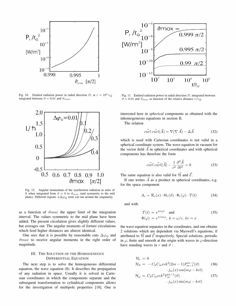
Fig. 10. Emitted radiation power in radial direction Pr at r = 105 rQintegrated between ϑ = 0.01 and ϑmax.

Fig. 11. Emitted radiation power in radial direction Pr integrated betweenϑ = 0.01 and ϑmax as function of the relative distance r/rQ.

Fig. 12. Angular momentum of the synchrotron radiation in units ofh when integrated from ϑ = 0 to ϑmax (and symmetric to the midplane). Different regions ±∆ϕQ were cut out around the singularity.

as a function of ϑmax the upper limit of the integrationinterval. The values symmetric to the mid plane have beenadded. The present circulation gives slightly different values,but averages out. The angular moments of former circulationswhich feed higher distances are almost identical.

One sees that it is possible by reasonable cuts ∆ϕQ andϑmax to receive angular momenta in the right order ofmagnitude.

III. THE SOLUTION OF THE HOMOGENEOUSDIFFERENTIAL EQUATION

The next step is to solve the homogeneous differentialequation, the wave equation (8). It describes the propagationof any radiation in space. Usually it is solved in Carte-sian coordinates in which the components separate and thesubsequent transformation to cylindrical components allowsfor the investigation of multipole properties [18]. One is

interested here in spherical components as obtained with theinhomogeneous equations in section II.

The relation

~curl ~curl( ~A) = ∇(∇ ~A)−∆ ~A (32)

which is used with Cartesian coordinates is not valid in aspherical coordinate system. The wave equation in vacuum forthe vector field ~A in spherical coordinates and with sphericalcomponents has therefore the form

~curl ~curl( ~A)− 1c2∂2 ~A

∂t2= 0 (33)

The same equation is also valid for ~H and ~E .If one writes ~A as a product in spherical coordinates, e.g.

for the space component

Ar = Rr(x) ·Θr(ϑ) · Φr(ϕ) · T (t) (34)

and with

T (t) = e±iωt and (35)Φ(ϕ) = e±imϕ, k = ω/c, kr = x

the wave equation separates in the coordinates, and one obtains2 solutions which are dependent via Maxwell’s equations, ifattributed to ~H and ~E respectively. Special solutions, periodicin ϕ, finite and smooth at the origin with waves in ϕ-directionhave standing waves in r and ϑ :

Hr = 0Hϑ = − CkCmeck2(2m− 1)Pm−1

m−1 (ϑ) (36)· jm(x) cos(mϕ− kct)

Hϕ = CkCmeck2Pm−1

m (ϑ) (37)· jm(x) sin(mϕ− kct)

Er = − CkCmek2

ε0(m+ 1)Pmm (ϑ) (38)

· jm(x)x

cos(mϕ− kct)

Eϑ = − CkCmek2

ε0

Pm−1m (ϑ)2m+ 1

(39)

· [(m+ 1)jm−1(x)−mjm+1(x)]· cos(mϕ− kct)

Eϕ =CkCmek

2

ε0

2m− 12m+ 1

Pm−1m−1 (ϑ) (40)

· [(m+ 1)jm−1(x)−mjm+1(x)])· sin(mϕ− kct) .

The Pmn (ϑ) are the Associated Legendre Functions, jn(x)are Spherical Bessel Functions [13] [14], and the factors infront are chosen to give the right dimensions. Ck and Cm arenormalization constants. The wave functions are unambiguousfor m = 1, 2, 3, . . ., and the separation constant k determinesthe size of the whole object. More details may be found inappendix A.

The general solution of this central wave is then a sumover all the harmonics m and over the wave numbers k, withthe coefficients Cm and Ck, chosen to satisfy the boundaryconditions. If the central wave should describe the propagationof the synchrotron radiation of a charge on the special circleassumed in chapter II then k is already fixed by eq.(26).

The Bessel functions subdivide the fields into shells withalternating field directions from one to the next. It is shownin Fig. 13(a) for j1(x), and the logarithmic plot in Fig. 13(b)demonstrate the decrease of the amplitude like 1/x at high x.This is true for all n. Only Er decreases with 1/x2.

A sketch of the fields ~H and ~E for m = 1 for the innermostshells is displayed in Fig. 14.

IV. THE SYNCHROTRON RADIATION AND THE CENTRALWAVE.

The eqs.(36) and (38) can describe the propagation ofany radiation in space: the strong radiation generated in theannihilation process as well as the synchrotron radiation ofthe circulating charge. If the electron would exist as a stableradiation object the current of the charge and the radiationwould influence each other: the emission of synchrotronradiation would generate a permanent central electromagneticbackground field which on the other hand would be absorbedagain by the charge and compensates the energy loss.

To simplify the discussion it is still assumed that the chargemoves on a circular track and the scattering by the radiationprocesses is neglected. For the central wave also the lowestmode m = 1 is considered for the moment.

The power of the synchrotron radiation in ϕ-direction andthe azimuthal power of the central wave must be the same in acomplete solution and are compared in Fig. 15. The horizontalaxis displays the distance x which is equivalent to r/rQ. Thesynchrotron radiation is integrated up to ϑ = 0.9π/2 andthe narrow peaks of the synchrotron radiation demonstrate thelarge content of higher harmonics. The Fourier analysis of theazimuthal component of the Poynting vector of Fig. 9 with

Fig. 15. Azimuthal power distribution dPϕ/dx of the synchrotronradiation and of the central wave with m = 1 and m = 3 as a functionof x (≡ r/rQ). The functions are arbitrarily scaled.

ϑ = 0.9π/2 yields e.g. a frequency distribution with a widthat half height of about 100 times the fundamental frequency.

The overlap of the radiation with the central wave isbest with the fundamental frequency (m = 1). The higherharmonics of the central background with higher m-valuesstart all at higher x. This is a hint that the synchrotron radiationis described with waves close to the fundamental frequency.

The standing wave in x-direction is governed by the slowdecrease of the Bessel functions. This contradicts the finiteangular momentum and the finite total energy of a finite radi-ation cloud if the central wave should describe the radiationcontent of a real electron.

The angular momentum of the circulating wave integratedup to xmax is displayed in Fig. 16. The scale of the angularmomentum is arbitrary because the coefficients Ck and Cmfor m = 1 were just chosen to be 1. The angular momentumincreases with xmax to infinity for a solution when m =1 only is used. A Fourier like expansion in ϕ is needed toyield a finite result. Already the addition of a counter rotatingcontribution with m = 3 and the coefficients C3/C1 = 0.056leads to a constant but still oscillating result. An inclusion ofterms with m = 2 and m = 4 had a minor effect. Higherterms could not be tested because of the limited accuracy ofthe computing program.

The electric and the magnetic energy of the central wavesum up to a constant energy density dE/dx respective to xas displayed in Fig. 17. This would lead to an infinite totalenergy.

Again an expansion is needed to obtain a finite value. Thefunctions (36) etc. may be considered as members of a Fourier-Bessel expansion [19] [20]:

f(r) =∑i

Aijm(ki r) =∑i

Bijm(λi x) (41)

This may obviously be applied at t = 0. If e.g. for m = 1j1(x) in Hθ(x) is substituted by the truncated function shownin Fig. 18 and expanded in the region 0 ≤ x ≤ 40 thesum contains 12 terms. But this replacement is not valid in

Fig. 13. The space parts for Hϑ,ϕ, Er and Eϕ given by the respective jn(x) are shown for m = 1 (a) in linear and (b) in logarithmic plots. The amplitudesdecrease with 1/x.

Fig. 14. Sketch of the H- and the E-field for m = 1. The spheres in a) on which H is located are also shown in b).

Fig. 16. Angular momentum of the central wave in units of hintegrated up to xmax. The label ”m=1” assigns the contributionof the special solution with m = 1 only. In ”m-1 - m-3” aspecial solution with m = 3 is subtracted. C1 = 1 was used.

Fig. 17. Energy density dE/dx of the electric (· · ·) and themagnetic field (−−) of the central wave, and the sum of both(solid line) as a function of x (vertical axes unscaled).

Fig. 18. j1(x) and the truncated function which were expandedin a Fourier-Bessel series.

Fig. 19. Total energy density dE/dx after the replacementof k in the central wave by λik and summed with coefficientsobtained by the Fourier-Bessel expansion obtained by thetruncation like in Fig. 18 .

general for the whole set of wave functions. These equationsare only satisfied if all occurrences of k are replaced by λik.Nevertheless one finds that the expansion leads also to a goodapproximation for the wave functions which is proven by thefinite total energy shown in Fig. 19.

V. THE MASSLESS CHARGE IN THE CENTRAL WAVE

It has been shown that the synchrotron radiation of arelativistic circulating charge generates a circulating electro-magnetic background field. The question is if on the other handthe background field guides the charge on a circular path andboth form an object even a finite one which can be called anelectron.

The simplest configurations have been assumed up to now:a charge moving on a circular track and a background fieldwith m = 1 and a single k-value. The discussions in sectionIV already showed that a superposition of waves should bepresent. It will be shown in this section how a charge maymove in such a central background field.

A charge moving in the central wave with velocity v sees aneffective electric field (~E +µ0~v× ~H) which forces the chargeto follow the field lines. This is possible by emitting radiationto balance the momentum, and the statistical emission andabsorption of radiation will result in deviations.

To trace the field lines a massless charge probe which moveswith speed of light and which just follows the effective fieldwas inserted. Its track under different conditions was recorded.

The various harmonics differ in the symmetry regarding ϕwhich results in different phase velocities. This velocity is cat the radius x = m.

Field lines have been traced for waves with m = 1, m = 2,and m = 3 and for many starting points. A smooth field linehas always been found for each condition in the mid planeϑ = π/2 and the field lines stayed in the mid plane if startedthere.

Four special field lines in the mid plane (ϑ = π/2) seen bya charge with |~v| = c are drawn for m = 1 in Fig. 20. The axesare the Cartesian coordinates (ξ, ψ) of x. There is the circularfield line with a radius of x = m = 1, the next one oscillatestowards the center, and the next oscillates around x = 2. Theone oscillating around x = 3 shows counter rotating loops.The small loops become more and more flat for field linesfurther outward. The field lines can cross each other becausethey are functions of the coordinates and of the velocities aswell.

The field lines for m = 2 and higher are similar but aremodified according to the different symmetry. A probe withopposite charge moves just at the same distance but oppositeto the origin.

Smooth field lines have also been obtained outside the midplain. They are similar to the ones already discussed but oscil-late vertically. The field line e.g. corresponding to the circularone in Fig. 20 is shown in Fig. 21(a) in a top view and in (b)in a side view as function of ϕ. The line starts horizontallyat the Cartesian coordinates of x (ξ, ψ, ζ) = (0,−0.98, 0.41)and oscillates down to ζ = 0.23. For comparison: field linesin the mid plane show oscillations in ζ of only 10−16 givenby the numerical accuracy.

Field lines below the mid plane are vertically mirror sym-metric.

One further example which corresponds to the innermostfield line in Fig. 20 is shown in Fig. 22. The line startshorizontally here at (ξ, ψ, ζ) = (0,−1.3, 1.3). A toroid is alsodrawn into the top view for better visualization.

4) Summation over harmonics and wave number : Thepictures in the previous section show that field lines withdifferent shape already exist in a wave with constant k andm = 1. A charge in this field will therefore also generatesynchrotron radiation of higher harmonics. On the other handhigher harmonics are also necessary if the total angular mo-mentum of the system should be finite and a superposition

Fig. 20. Four selected closed effective electric field lines in the centralwave with m = 1 seen by a charge moving with |~v| = c. The circularone has a radius of x = 1. The innermost oscillates towards the center,one oscillates around x = 2, and the outer one at x = 3 showscounter rotating loops. Shown is the mid plane ϑ = π/2 in Cartesiancoordinates of x (ξ, ψ).

Fig. 21. Effective field line drawn by a massless test charge in the central wave with m = 1 above the mid plane. The line starts horizontally at the Cartesiancoordinates (ξ, ψ, ζ) = (0,−0.98, 0.41). Fig.(a) shows the line in the top view, and Fig.(b) displays the vertical oscillation as a function of ϕ. Field linesbelow the mid plane are vertically mirror symmetric.

Fig. 22. Effective field line above the mid plane corresponding to the innermost field line of Fig. 20. It starts horizontally at (ξ, ψ, ζ) = (0,−1.3, 1.3). Atoroid is inserted in the top view for better visualization.

with different wave numbers ki = λik is necessary for a finiteenergy as discussed in section IV.

The field lines in a wave with m = 1 and m = 3 whichlead to a finite angular momentum (Fig. 16) are unchangedbelow x = 2 but are deformed at higher distances from thecenter but they are all still smooth.

Field lines in a wave described by the example of a Fourier-Bessel expansion in Fig. 18 are also still smooth but radiallyoscillating.

It is the description of the synchrotron radiation by thecentral wave with finite solutions which will finally select theproper superposition.

VI. ON THE MASS OF THE ELECTRON

The electric field of a moving electron transports energyas well as momentum. The energy of the rest mass mec

2 isgenerally assumed to equal the self-energy of a suitable chargedistribution. The kinetic energy of a moving charge, on theother hand, yields different mass energies via the momentumcalculated with the Poynting vector and via the energy of themagnetic field of the current. This is in contradiction to specialrelativity [6].

One may expect that under Lorentz transformation e.g.in the x1-direction the energy transforms like E = γEand the momentum like (p1, p2, p3) = (βγp1, p2, p3) andE2 − (pc)2 = E2 − (pc)2 = (mc2)2 should yield the massof the object. This is not true in general because energy andmomentum of the field don’t form a 4-vector. They belong toan energy-momentum tensor Tµν [21] [22] [23]. With

T00 = ρE =ε02~E2 +

µ0

2~H2; (42)

T0i = −ρP0i c = −Si/c ;

Tik = ε0(12~E2δik − EiEk)

+µ0(12~H2δik −HiHk) ;

i, k = 1 . . . 3, and Tµν = Tνµ

ρE , ρP0i are the energy and momentum densities of the field,~S the Poynting vector, and Tik Maxwell’s tension tensor. Thetrace of the tensor vanishes in the rest system of the fields.

Lorentz transformation yields then the energy and momen-tum of a conventional charge moving with velocity v/c = β

Eβ =∫ρEβd3xβ (43)

=1γ

∫(γ2T00 + (γ2 − 1)T11)d3x ,

pβ1 c =∫ρPβ1 d3xβ

= −βγ∫

(T00 + T11)d3x ,

pβ2,3 =∫ρPβ2,3d

3xβ

= −β∫

(T12,3)d3x = 0 ,

and for the rest mass from the field squared

Eβ2 − ~pβ

2c2 (44)

= γ2

[∫(T00 + β2T11)d3x

]2− β2γ2

[∫(T00 + T11)d3x

]2.

Variables without the superscript β indicate that they are inthe rest frame.

Neither the field energy nor its momentum show the properdependence on γ and the rest mass is not constant. Thereason is that with this concept one has to introduce a chargedistribution at the origin of the electron to avoid the singularityof Coulomb’s law [23]. Inner forces result which have to besomehow compensated. One must require T11 = 0 if eq.(44)should be valid at any particle speed.

The situation in the present model is different: there existsa charged radiation bucket which moves with β = 1. The fieldenergies are again the self energies with the singularity cut out.If one takes a differential section of the circular path wherethe charge moves in the 1-direction eq.(44) becomes now

Eβ2 − ~pβ

2c2 = γ2

[∫(T00 + T11)d3x

]2(45)

− β2γ2

[∫(T00 + T11)d3x

]2=[∫

(T00 + T11)d3x

]2.

This is constant and may be defined as the mass energy of thecharge mq c

2.

mq c2 =

23ε0

∫~E2d3x (46)

In addition there is the energy of the standing wave of thecentral wave background and of the quantum mechanic centermw c

2. Both add then to the total mass energy of the electron

me c2 = mq c

2 +mw c2 . (47)

VII. CONCLUSION

The presented investigations suggest that the classical elec-tron can be described by a circulating massless charge field.

The comparison with the experimental properties of theelectron show that already a movement on a circular trackresults in a good consistency. The radius of the circulationresults from the experimental value of the magnetic momentand is obtained to rQ = 3.81 10−13 [m]. It represents also thesize of the object.

The values for the circulation frequency and the Comptonwavelength follow directly, and with Planck’s constant h themass of the electron is reproduced.

A small volume around the singularity of the charge field isrequired in which strong radiation processes lead to quantummechanical effects. This volume has to be cut out in the presentclassical considerations.

The circulating charge emits synchrotron radiation and whenmoving with speed of light it is totally embedded in thisradiation. The static field around the quantum mechanicalvolume vanishes and this part becomes neutral.

The angular momentum L/h of the synchrotron radiation ofthis charge moving on a circle with radius rQ yields reasonablevalues of the order of 1 as expected from the spin of theelectron. Its value depends on the cuts by which the quantummechanical region is removed and finally on the real path onwhich the charge is moving.

The mean electric field of the synchrotron radiation repro-duces the Coulomb field. The field is however not sphericalsymmetric but it dominates close to the plane of circulation.

The solution of the homogeneous wave equation describesthe propagation of the electromagnetic waves in vacuum. Thisbackground field may be formed during the creation process ofthe charge and be maintained by the synchrotron radiation ofthe charge. When evaluated in a spherical coordinate system itleads to a central radiation background with a special solutionwhich moves in ϕ-direction but with standing waves in ϑ andr.

The central wave field can carry the massless charge ontracks around the origin. It generates smooth electric fieldlines e.g. a circular one but in general these are oscillating inspace. The charge tries to follow these field lines by emittingsynchrotron radiation and this radiation is guided back by thecentral wave and forms a feed back system which compensatesthe energy loss in ϕ-direction. Fast oscillations will be dampedand the interaction will select the configuration with the lowestenergy.

The standing wave of the background field in r-direction forthe special solution of m = 1 extents to infinity and leads toan infinite total angular momentum and an infinite total energyof the central wave. A 2-dimensional Fourier like expansionof the wave functions in ϕ and x may form a finite solution.An admixture of an m = 3 contribution leads already to afinite angular momentum and an example of a Fourier-Bessellike expansion in x lead to a finite energy too.

The synchrotron radiation bucket moves with β = 1. Theinner tensions which normally occur at lower speed if one cutsout the singularity disappear now. A constant mass energycompatible with the relativistic energy-momentum tensor ofthe field results.

Thus one finds, that the electron may totally be describedby the synchrotron radiation of a massless charge field. It doesnot only behaves like a wave, it is a wave.

APPENDIX

Solving the homogeneous wave equation in spherical coordi-nates

The wave equation

~curl ~curl( ~F) = − 1c2∂2 ~F∂t2

(48)

is solved in spherical coordinates for a vector field ~F to yielddirectly the spherical components of the field. The equation is

expected to separate in the variables when a product ansatz ismade, e.g. for Fr:

Fr = Ar · Rr(x) ·Θr(ϑ) · Φr(ϕ) · T (t) (49)

and with

T (t) = e±iωt and (50)Φ(ϕ) = e±imϕ, k = ω/c , kr = x .

One expects a source free wave field and may thus subtract~∇(~∇ ~F) in eqn. (48) as one does in Cartesian coordinates. Thissimplifies the equation, but has to be checked afterwards. Theansatz eqn. (50) eliminates the time and ϕ-dependence in theequation and the 3 following components remain:

−ArΘr(ϑ) ∂∂x

1x2

∂∂xx

2Rr(x)−Ar Rr(x)

x2 sin(ϑ)2 Θr(ϑ)· (x2 sin(ϑ)2 −m2)

−Ar Rr(x)x2 sin(ϑ)

∂∂ϑ sin(ϑ) ∂

∂ϑΘr(ϑ)

Aϑ2Rϑ(x)x2

· ( cos(ϑ)sin(ϑ) Θϑ(ϑ) + ∂

∂ϑΘϑ(ϑ))

+Aϕ2m Rϕ(x)x2 sin(ϑ)Θϕ(ϑ)

= 0 , (51)

2ArRr(x) ∂∂ϑΘr(ϑ)

+AϑΘϑ(ϑ) ∂∂xx

2 ∂∂xRϑ(x)

+AϑRϑ(x)· ∂∂ϑ

1sin(ϑ)

∂∂ϑ sin(ϑ)Θϑ(ϑ)

−AϑRϑ(x)Θϑ(ϑ)( m2

sin(ϑ)2 − x2)

−2mAϕRϕ(x) cos(ϑ)sin(ϑ)2 Θϕ(ϑ)

= 0 , (52)

2ArRr(x)Θr(ϑ) msin(ϑ)

+2mAϑRϑ(x) cos(ϑ)sin(ϑ)2 Θϑ(ϑ)

−AϕΘϕ(ϑ) ∂∂xx

2 ∂∂xRϕ(x)

−AϕRϕ(x) 1sin(ϑ)

· ∂∂ϑ sin(ϑ) ∂∂ϑΘϕ(ϑ)

+AϕRϕ(x)Θϕ(ϑ)( m2+1

sin(ϑ)2 − x2)

= 0 . (53)

One obtains special solutions if one chooses

Rϑ(x) = jnϑ1(x) + aϑjnϑ1+1x (x)

Rϕ(x) = jnϕ1(x) + aϕjnϕ1+1(x)

x

(54)

Θr(ϑ) = P qp (ϑ)Θϑ(ϑ) = P qp (ϑ)Θϕ(ϑ) = P qp (ϑ))

(55)

and uses

1sin(ϑ)

∂

∂ϑsin(ϑ)

∂

∂ϑPmn (ϑ) (56)

=[

m2

sin(ϑ)2− n(n+ 1)

]Pmn (ϑ) ,

∂

∂xx2 ∂

∂xjn(x) = [n(n+ 1)− x2]jn(x) .

If one eliminates Rr(x) from both eq. (52) and eq. (53),and sets nϑ = nϕ one arrives at

mPmp (ϑ)

sin(ϑ) ∂∂ϑP

mp (ϑ)

·

Aϑ( ∂∂xx

2 ∂∂xRϑ(x))Pµν (ϑ)

AϑRϑ(x)· ∂∂ϑ

1sin(ϑ)

∂∂ϑ sin(ϑ)Pµν (ϑ)

−AϑRϑ(x)Pµν (ϑ)· ( m2

sin(ϑ)2 − x2)

−2AϕmRϕ(x) cos(ϑ)sin(ϑ)2P

ML (ϑ)

2mAϑRϑ(x)Pµν (ϑ) cos(ϑ)sin(ϑ)2

−Aϕ( ∂∂xx

2 ∂∂xRϕ(x))PML (ϑ)

+AϕRϕ(x)PML (ϑ)[m2−M2+1sin(ϑ)2

+ L(L+ 1)− x2]

= 0 . (57)

One gets now 2 solutions for eq. (57). One for which boththe upper and lower cluster vanish separately, and the otherone for which the left side of this equation vanishes on thewhole.

When these results are inserted into equ. (51) they determineRr(x), and div( ~F) = 0 restricts the values of the separationconstants. Both solutions may represent solutions of the elec-tromagnetic fields ~E and ~H.

ACKNOWLEDGMENT

A presentation of an early version of this paper to E.Lohrmann showed the regions which have to be furtherdeepened. I am grateful to K. Fredenhagen for many detaileddiscussions. Without the patience and the confidence of mywife Ursula this work would not exist.

REFERENCES

[1] A. O. Barut, Brief History and Recent Developments in ElectronTheory and Quantumelectrodynamics in The Electron New Theory andExperiment (D. Hestenes and A. Weingart, Editors; Springer, 1991) p.105

[2] L. de Broglie, Nonlinear Wave Mechanics (Elsevier, Amsterdam 1960)p. 6

[3] J. Orear, Jay Orear Physics (Macmillan, New York 1979)) Chp. 18-4[4] M. Alonso, E.J. Finn, Fundamental University Physics II (Addison-

Wesley, Amsterdam 1974) 515[5] M. H. McGregor, The Enigmatic Electron (Kluwer Academic, Dortrecht

1992)[6] A. Sommerfeld, Electrodynamics: Lectures on Theoretical Physics (Aca-

demic Pr., New York 1952) §33[7] P. A. M. Dirac, Proc. Roy. Soc. London A268, (1962) 57[8] H. Jehle, Phys. Rev. D15, (1977) p. 3727 and citations there.[9] A. O. Barut and N. Zanghi, Phys. Rev. Lett. 52, (1984) 2009

[10] Qiu-Hong Hu, Physics Essays, 17, (2004) 442[11] J. G. Williamson and M.B. van der Mark, Ann. de la Foundation Louis

de Broglie 22, (1997) 133[12] L. D. Landau and E. M. Lifshitz The Classical Theory of Fields

(Butterworth-Heinemann, Oxford 2000) 2, Chp. 8[13] Handbook of Mathematical Functions (editors: M. Abramovitz and I.A.

Stegun; National Bureau Std., Appl. Math. Series 55, Washington 1966)Chp. 8, Chp. 10

[14] P. M. Morse and H. Feshbach, Methods of Theoretical Physics (McGraw-Hill, New York 1953) Chp. 10, Chp. 11

[15] D. Iwanenko and A. Sokolov Klassische Feldtheorie (Akademie-Verlag,Berlin 1953) §39

[16] W. Greiner Classical Electrodynamics (Springer New York 1996) §21[17] J. D. Jackson Classical Electrodynamics (Wiley, New York 1975) Chp.

14[18] J. D. Jackson ibid. Chp. 16[19] I. N. Sneddon Special Functions of Mathematical Physics and Chemistry

(Oliver and Boyd, Edinburgh 1961) §35[20] A. Sommerfeld, Partial Differential Equations In Physics: Lectures On

Theoretical Physics (Academic Pr., New York 1952) §20, and exerciseV.1

[21] [17] Chp. 17[22] [15] §29 - §30[23] R. U. Sexl and H. K. Urbantke Relativity, Groups, Particles (Springer,

Wien 2001) Chp. 5.10