on the virtual element method for three-dimensional linear

Available online at www.sciencedirect.com

ScienceDirect

Comput. Methods Appl. Mech. Engrg. 282 (2014) 132–160www.elsevier.com/locate/cma

On the Virtual Element Method for three-dimensional linearelasticity problems on arbitrary polyhedral meshes

Arun L. Gain1, Cameron Talischi1, Glaucio H. Paulino∗

Department of Civil & Environmental Engineering, University of Illinois at Urbana-Champaign, USA

Available online 29 May 2014

Abstract

We explore the recently-proposed Virtual Element Method (VEM) for the numerical solution of boundary value problemson arbitrary polyhedral meshes. More specifically, we focus on the linear elasticity equations in three-dimensions and elaborateupon the key concepts underlying the first-order VEM. While the point of departure is a conforming Galerkin framework, thedistinguishing feature of VEM is that it does not require an explicit computation of the trial and test spaces, thereby circumventinga barrier to standard finite element discretizations on arbitrary grids. At the heart of the method is a particular kinematicdecomposition of element deformation states which, in turn, leads to a corresponding decomposition of strain energy. By capturingthe energy of linear deformations exactly, one can guarantee satisfaction of the patch test and optimal convergence of numericalsolutions. The decomposition itself is enabled by local projection maps that appropriately extract the rigid body motion and constantstrain components of the deformation. As we show, computing these projection maps and subsequently the local stiffness matrices,in practice, reduces to the computation of purely geometric quantities. In addition to discussing aspects of implementation of themethod, we present several numerical studies in order to verify convergence of the VEM and evaluate its performance for varioustypes of meshes.c⃝ 2014 Elsevier B.V. All rights reserved.

Keywords: Virtual Element Method; Mimetic Finite Difference; Polyhedral meshes; Polytopes; Voronoi tessellations

1. Introduction

The development of discretization methods for solving three-dimensional boundary value problems on generalpolyhedral meshes has recently received considerable attention in the numerical analysis literature. One driving forcebehind this trend is the difficulty associated with mesh generation for complex or evolving domains, for which theuse of arbitrarily-shaped elements can provide much needed flexibility [1]. For example, a simple embedding strategyconsisting of carving out the problem domain out of a structure background grid, produces polyhedral elements atthe boundary [2]. Mesh refinement and coarsening in adaptive schemes can also be handled with greater ease if the

∗ Corresponding author. Tel.: +1 217 333 3817; fax: +1 217 265 8041.E-mail address: [email protected] (G.H. Paulino).

1 Equal contribution authors.

http://dx.doi.org/10.1016/j.cma.2014.05.0050045-7825/ c⃝ 2014 Elsevier B.V. All rights reserved.

http://crossmark.crossref.org/dialog/?doi=10.1016/j.cma.2014.05.005&domain=pdf

http://www.elsevier.com/locate/cma

http://dx.doi.org/10.1016/j.cma.2014.05.005

http://www.elsevier.com/locate/cma

mailto:[email protected]

http://dx.doi.org/10.1016/j.cma.2014.05.005

A.L. Gain et al. / Comput. Methods Appl. Mech. Engrg. 282 (2014) 132–160 133

analysis method allows for the presence of elements with general geometries [3]. In addition to advantages in meshgeneration and adaptation, polyhedral discretizations can deliver improved performance in some applications. Forexample, as discussed in [4], polyhedral meshes can achieve the same level of accuracy in flow simulations comparedto their simplicial counterparts but with far fewer number of cells and unknowns.

With regards to the type of discretization method, finite volume methods based on polyhedral cells have reached alevel of maturity in fluid dynamic simulations, as evidenced by their availability and use in commercial software [5,6].Mimetic finite difference (MFD) methods, capable of handling general three-dimensional meshes, are also the subjectof active research and have been successfully applied to diffusion, elasticity, and fluid flow problems (see, forexample, [7–11]). The extension of finite element methods in this arena, however, has been relatively slow, despite theavailability of special interpolation functions in the literature. This is, in part, due to the fact that these interpolantsare subject to restrictions on the geometry of admissible elements (e.g., convexity, maximum valence count) and canbe sensitive to geometric degeneracies. More importantly, calculating these functions and their gradients are oftenprohibitively expensive. Numerical evaluation of weak form integrals, with sufficient accuracy, poses yet anotherchallenge due to the non-polynomial nature of these functions as well as the arbitrary domain of integration2 [12].To mention a few approaches in the literature aiming to overcome these barriers, we point to the work by Rashid andco-workers [13,2,3], who have developed elements based on non-conforming polynomial or piecewise polynomialbasis functions that are tolerant of degeneracies. More recently, harmonic basis functions have been consideredby [14,15] with particular attention to alleviating the cost of their computation and integration. Other works includeconstructions based on natural element [16], non-Sibson [17], and mean value coordinates [18], the smoothed finiteelement method [19], and the extension of the so-called mean-quadrature approach to polyhedral grids [20].

In this work, we focus on the recently-developed Virtual Element Method (VEM) that addresses some of theabove-mentioned challenges facing finite element schemes [21–24]. As with finite elements, VEM is a Galerkinscheme with an underlying approximation space defined according to a partition (mesh) of the domain. However, it isdistinguished from classical finite elements in that it does not require the computation of the interpolation functions inthe interior of the elements. One goal of the present work is to break down and elaborate upon the core mathematicalconcepts underlying VEM within the context of linear elasticity boundary value problems. The key to the success ofthe method is a consistent approximation to the elemental strain energy that is exact for the linear deformations withoutrequiring volumetric integration of the basis functions. What enables this approximation is a set of local projectionmaps that appropriately split up the element deformation into its polynomial and non-polynomial components. Inthe case of the first-order VEM formulation, where the degrees of freedom are associated with the vertices of theelements, two projection maps, associated with rigid body motion and constant strain deformations, respectively, areused to achieve this kinematic decomposition. As we shall discuss, these projection maps can be beneficial even forfinite element schemes when one has access to interpolation functions. We should note that while VEM provides thegeneral recipe for extension to higher-order and higher-continuity polyhedral elements (see, for example, [25]), thissignificant technology may be hidden in this paper as we will limit the discussion, for the sake of clarity, to the first-order formulation. We refer to [22] for a discussion of arbitrary order VEM for both compressible and incompressibleelasticity in two dimensions.

The other task undertaken here is to discuss, in detail, aspects of the implementation of the method for generalpolyhedral meshes. To this effect, we will derive explicit expressions for the element stiffness matrix and discreterepresentation of the element projection maps. In addition to two matrices containing special arrangements ofcoordinates of the element vertices, we encounter two matrices that require calculation of surface integrals of the basisfunctions over the element boundary. These quantities also reduce to geometric information of the faces (centroids,areas, etc.), if either the approximation spaces are based on interpolants derived by [26] or if a consistent nodalquadrature rule is used. While the connection between the MFD method and VEM has been established in the originalpapers on VEM, the discussion here further elucidates this relationship and illustrates how the Galerkin frameworkwith an underlying approximation space serves as a vehicle for constructing a method that is ultimately geometricin nature. Finally, we note that the recent work [24] also discusses practical aspects of implementation of VEM forsecond-order elliptic problems in two and three dimensions.

2 By contrast, classical finite elements feature interpolation functions that are either polynomials or images of polynomials and numericalintegration is carried out by means of a mapping to a fixed parent domain.

134 A.L. Gain et al. / Comput. Methods Appl. Mech. Engrg. 282 (2014) 132–160

The remainder of this paper is organized as follows. In Section 2, we define the three-dimensional elasticity modelproblem and its Galerkin approximation on a polyhedral mesh. Section 3 presents the VEM formulations and itstheoretical underpinning. Next, in Section 4, we derive explicit and simplified expressions for the element stiffnessmatrices and discuss aspects of implementation of the method. We evaluate the performance of VEM in Section 5 viaseveral numerical studies and conclude the work with some remarks in Section 6.

We follow fairly standard notation throughout the paper. As usual, Sobolev spaces H k(Ω) consist of functionswhose weak derivatives up to the kth order are square-integrable on Ω . The norm on this space, as well as itsvector-valued counterpart H k(Ω)3, is denoted by ∥·∥k,Ω . We denote the symmetric gradient operator by ϵ(·) =∇ · +∇

⊤·/2 and the skew-symmetric gradient by ω(·) =

∇ · −∇

⊤·/2. Also, Im represents the m × m identity

matrix. We shall denote the components of vectors, matrices and tensors in the canonical Euclidean basis withsubscripts inside parentheses (e.g. v(i) or ϵ(i j)) in order to make a distinction with indexed quantities. Finally, weuse |·| to denote the measure (area or volume) of a set as well as the Euclidean norm of a vector.

2. Model problem and discretization

Consider a linear elastic body, with constant stiffness tensor C, occupying a smooth bounded domain Ω ⊆ R3

whose boundary ∂Ω is partitioned into disjoint non-trivial segments Γu and Γt (i.e., Γu ∪ Γt = ∂Ω , Γu ∩ Γt = ∅ and|Γu| = 0). The body is subjected to body forces b in Ω , surface tractions t on Γt, and applied displacements g on Γu,with all fields assumed to have sufficient regularity (cf. Fig. 1). The resulting deformation u is the unique minimizerof the total potential energy:

u = argminv∈V g

12

a(v, v) − f (v). (1)

Here, V g=v ∈ H1(Ω)3

: v = g on Γu

is the space of kinematically admissible displacement fields and

a(u, v) =

Ω

σ (u) : ϵ(v)dx, f (v) =

Ω

b · vdx +

Γt

t · vds (2)

are the energy bilinear form and load linear form, respectively. In the above expression, σ (u) denotes the stress fieldassociated with u, that is,

σ (u) = Cϵ(u). (3)

Observe that due to the symmetries of C, the bilinear form is symmetric in its arguments. We shall assume throughoutthe paper that the exact solution u is a smooth function (e.g. belongs to H2(Ω)3).

2.1. Galerkin approximation

Consider a partition Th of Ω into disjoint non-overlapping polyhedra with maximum diameter h. For theoreticalreasons, it is assumed that Th satisfies some mild shape regularity assumptions. As discussed in [26] (see also[27,10]), it is sufficient if, for example, there exists ς > 0 such that for every E ∈ Th , face every F of E andevery edge e of F (i) diam(e) ≥ ςdiam(F) ≥ ς2diam(E), (ii) E is star-shaped with respect to points in a ball ofradius of ςdiam(E), (iii) F is star-shaped with respect to points in a disk of radius ςdiam(F).

We define a conforming discrete space Vh consisting of continuous displacement fields whose restriction to E ∈ Thbelongs to the finite-dimensional space W(E) of smooth functions. Thus,

Vh =

v ∈ C0(Ω)3

: v|E ∈ W(E) for all E ∈ Th

. (4)

Here, the space W(E) contains the deformation states that can be represented by the element E . Note that C0-continuity along with the requirement that W(E) ⊆ H1(E)3 implies Vh is a subspace of H1(Ω)3. Moreover, theusual requirement that W(E) includes linear displacement fields (or equivalently that E can represent rigid bodymotions and constant states of strains) furnishes the first-order approximation property of Vh , namely that sufficiently


a b

c d

Fig. 1. (a) Schematic illustrating the elasticity boundary value problem. (b) Partition Th of the domain Ω . (c) Split view of the discretized domain.(d) View of a few boundary and internal elements.

smooth displacement fields, including the solution of the continuous problem (1), can be approximated by elementsof Vh with O(h) errors in the energy norm3 [28,26].

The Galerkin approximation uh of u is obtained by replacing V g with the discrete space of admissible displacementsgiven by

V gh = V g

∩ Vh (5)

in the minimization problem (1). Therefore,

uh = argminv∈V g

h

12

a(v, v) − f (v). (6)

We are assuming here that the essential boundary conditions can be satisfied exactly in Vh since otherwise theintersection in (5) will be empty. In practice, the boundary data g is replaced by its nodal approximation gh butthe analysis of the effects of this error is classical [28] and so we shall ignore it to simplify the presentation.

3 The energy norm is equivalent to the H1-norm in the space V 0.


Fig. 2. Decomposition of the faces of polyhedron into Fi and F ci . Here, Fi represents the set of faces containing vertex xi and F c

i represents theremaining faces.

Due to the conformity of Vh , the strain energy associated with v ∈ Vh is simply the sum of the contributions fromthe elements in the mesh. In other words,

a(v, v) =

E∈Th

aE (v, v) (7)

where we have denoted by aE the strain energy associated with element E given by

aE (u, v) =

E

σ (u) : ϵ(v)dx. (8)

As we will see, particular attention will be given in VEM to an appropriate approximation of these local strain energiesthat in turn determine the energetic behavior of the polyhedral elements. Naturally, this will first require a descriptionof the element space W(E), which as discussed in the next section, will be a typical nodal finite element space.

2.2. Construction and properties of W(E)

As stated before, each element E ∈ Th is a polyhedron whose boundary consists of planar polygonal faces.Suppose E has n vertices located at x1, . . . , xn . Let us denote by F E the set of faces forming the boundary of E ,by Fi those faces that include xi , and by F c

i = F E \ Fi the remaining faces (see Fig. 2). Note that we do notrequire E to be convex though convexity and its implications on the mesh geometry can simplify certain aspects ofimplementation.

We will give a construction of the element space W(E) with three degrees of freedom associated with each vertex.To this effect, we consider the canonical basis ϕ1, . . . ,ϕ3n of the form

ϕ3i−2 = [ϕi , 0, 0]⊤ , ϕ3i−1 = [0, ϕi , 0]⊤ , ϕ3i = [0, 0, ϕi ]⊤ , i = 1, . . . , n (9)

where ϕ1, . . . , ϕn constitutes a set of barycentric coordinates for E . Examples of barycentric coordinates for polytopescan be found in [29–32]. Among these, we will use the maximum entropy coordinates [31] later in our numericalstudies. By definition, barycentric coordinates satisfy the Kronecker-delta property (i.e., ϕi (x j ) = δi j ), which inturn implies that each u ∈ W(E) is completely characterized by the values it assumes at the vertices of element E ,consistent with the stated choice of degrees of freedom. Furthermore, ϕi varies linearly along the edges of E andvanishes on F c

i , i.e., the faces not incident on the associated vertex xi . Also, the variation of ϕi on the faces in Fiis determined uniquely by the geometry of those faces and independent of the shape of the element. The latter twoproperties are crucial in guaranteeing inter-element continuity, and subsequently conformity of Vh , as the variation ofu ∈ W(E) on a face is uniquely determined by values of u at vertices of that face and its geometry. Finally, barycentric


coordinates can interpolate linear fields exactly, that is,

a + b · x =

ni=1

(a + b · xi ) ϕi (x) (10)

for any a ∈ R and b ∈ R3. This, in turn, implies that the element E can represent rigid body motions and states ofconstant strain, i.e.,

W(E) ⊇ P(E).=

a + Bx : a ∈ R3, B ∈ R3×3

(11)

guaranteeing the previously-stated first-order approximation capability of W(E). We should note that if E isa tetrahedron, the well-known linear shape functions are the unique set of barycentric coordinates for E andW(E) = P(E).

As we will see in the next section, what is more relevant in VEM is the behavior of functions in W(E) on theboundary, not in the interior of E . Therefore, it is imperative to know the boundary behavior of the barycentriccoordinate defining the basis functions (9). A useful observation is that, given any two-dimensional barycentric co-ordinates for planar polygons, we can use harmonic lifting to construct barycentric coordinates for E exhibiting theabove-mentioned properties. This process defines ϕi as the solution to the Laplace equation whose boundary condi-tions are set to be the two-dimensional barycentric coordinates on faces in Fi and zero on the faces in F c

i (see Fig. 2).The resulting coordinates ϕi ’s will have the desired boundary behavior (Kronecker-delta property at the vertices, lin-earity and continuity along edges, and variation on the faces dictated by the choice of 2D barycentric coordinates),and their linear completeness follows from the linear completeness of 2D coordinates and properties of Laplace’sequation. We remark that the use of harmonic basis have been explored in practice (see, for example, [15,14]).

Later we shall assume the use of this harmonic construction of W(E) along with a particular set of boundarycoordinates defined in [26], which possess the useful property that their average value can be computed explicitlybased on the geometry of the underlying polygon (see the Appendix for more details). If instead a nodal quadraturerule is used for computing surface integral encountered in the formulation, no distinction will be made betweendifferent barycentric coordinates (harmonic or otherwise) underlying W(E) (cf. Section 4).

We close this section by recalling the quasi-optimality of the error in the Galerkin solution, namely that the Galerkinerror is bounded by a constant multiple of the error in the best approximation of u in V g

h (cf. Cea’s lemma, Theorem2.4.1 in [33]):

∥u − uh∥1,Ω ≤ C infwh∈V g

h

∥u − wh∥1,Ω . (12)

By the approximation property of the finite element space and regularity of u, the right hand side is O(h), and theconvergence rate is linear.

3. Virtual Element Method (VEM)

While the Galerkin discretization on Th is now completely defined, its realization is difficult to achieve in practice.One source of difficulty is the evaluation of the weak form integrals, i.e., computing aE and f . Since the functions inW(E), and in particular its basis, are in general non-polynomial functions, available quadrature rules will inevitablylead to errors in the evaluation of the weak form integrals. Using high-order quadrature rules to reduce this error toacceptable levels is prohibitively expensive in practice since the construction of the basis functions (harmonics orotherwise), due to the lack of availability of explicit analytical expressions, is computationally costly.

Acknowledging the presence of error in the evaluation of the linear and bilinear forms, we find ourselvescommitting a variational crime and deviating from the Galerkin framework, in effect replacing a, aE and f byapproximate mesh-dependent counterparts ah , aE

h and fh , respectively. The resulting approximate solution uhminimizes the discrete total potential energy and is characterized by

uh = argminv∈V g

h

12

ah(v, v) − fh(v). (13)


We can analyze the error u − uh by using the Galerkin solution uh as an intermediary as follows:

∥u − uh∥1,Ω ≤ ∥u − uh∥1,Ω + ∥uh − uh∥1,Ω . (14)

As before, the first term is governed by the approximation properties of the discrete space (cf. (12)). The secondterm represents the consistency error introduced by replacing the total potential energy by its discrete counterpart.According to Strang’s lemma (cf. Lemma 4.1 and Theorem 4.1 of [28]), provided that ah is uniformly coercive on V 0

h ,we have the following bound for this term:

∥uh − uh∥1,Ω ≤ C supv∈V 0

h

|a (uh, v) − ah (uh, v)| + | f (v) − fh(v)|∥v∥1,Ω

. (15)

Here, C is a constant independent of h. If the discrete strain energy and load forms are defined such that the terms inthe consistency error (15) are O(h), we can ensure that uh converges to u at the same (optimal) rate as the Galerkinsolution uh .

As before, within the conforming setting, the discrete energy bilinear form ah is typically obtained from thecontribution of the discrete elemental bilinear forms

ah(v, v) =

E∈Th

aEh (v, v). (16)

As detailed in the remainder of this section, the virtual element method, first introduced in [21], gives a particularconstruction of aE

h such that aEh (v, v) and its variations are exact whenever v is either rigid body motion or a constant-

strain displacement field on E . In other words, each element in the mesh will correctly represent the strain energyassociated with these deformation states. This means that the patch test will be passed at the element level. Theconsequence of the satisfaction of the element patch test, as discussed in Section 3.2, is that the consistency errorintroduced by replacing a by ah (i.e., the first term in (15)) is O(h). Curiously, the construction of the discrete bilinearforms ah

E in VEM does not require numerical quadrature inside the element and therefore eliminates the need forcostly computation of the basis functions in the interior of the element.

3.1. Kinematics decomposition of W(E)

We now discuss a particular kinematic decomposition of the deformation states in W(E) that is central to the VEMconstruction. In the remainder of this subsection, we will focus on element E ∈ Th and thus omit the dependence onE to ease the notation (e.g. write W for W(E) and P for P(E)). For a function w, we shall denote by w the mean ofthe values it assumes over the vertices of E :

w =1n

ni=1

w(xi ). (17)

This means, for example, that x is the geometric center of E . Similarly, we will use ⟨·⟩ to denote the volume averageover E :

⟨w⟩ =1

|E |

E

wdx. (18)

First let us split up P , the space of linear displacements over E , into the spaces of rigid body motions and constantstrain modes, defined, respectively, by

R =

a + BA (x − x) : a ∈ R3, BA ∈ R3×3, B⊤

A = −BA

(19)

C =

BS (x − x) : BS ∈ R3×3, B⊤

S = BS

. (20)

Observe that P is a direct sum of R and C, and by (11), R and C are subspaces of W . We next define bases for thesespaces, respectively denoted by r1, . . . , r6 and c1, . . . , c6, as follows. We set r1, r2, r3 to be rigid body translation


modes and r4, r5, r6 pure rotations about x:

r1(x) = [1, 0, 0]⊤ r4(x) =(x − x)(2) , − (x − x)(1) , 0

⊤r2(x) = [0, 1, 0]⊤ r5(x) =

0, (x − x)(3) , − (x − x)(2)

⊤ (21)

r3(x) = [0, 0, 1]⊤ r6(x) =− (x − x)(3) , 0, (x − x)(1)

⊤.

Similarly, we choose c1, c2, c3 to correspond to deformation modes with constant axial strains, and c4, c5, c6 torepresent three constant shear strains:

c1(x) =(x − x)(1) , 0, 0

⊤ c4(x) =(x − x)(2) , (x − x)(1) , 0

⊤c2(x) =

0, (x − x)(2) , 0

⊤ c5(x) =0, (x − x)(3) , (x − x)(2)

⊤ (22)

c3(x) =0, 0, (x − x)(3)

⊤ c6(x) =(x − x)(3) , 0, (x − x)(1)

⊤.

In these expressions, the subscript within parentheses designates the component of the associated vector. The basesfor R and C are illustrated for an arbitrary polyhedron in Fig. 3.

Next we define projection maps πR : W → R and πC : W → C that allow us to extract the rigid body motionand constant strain part of any deformation state v ∈ W . By definition, these maps will satisfy

πRr = r, ∀r ∈ R (23)

πC c = c, ∀c ∈ C. (24)

Moreover, it will be useful to require the following orthogonality conditions:

πRc = 0, ∀c ∈ C (25)

πC r = 0, ∀r ∈ R (26)

reflecting the fact that elements of C will contain no rigid body motions and, similarly, elements of R will be associatedwith null element in C. Subsequently, πC πR = πRπC = 0 and

πP = πR + πC (27)

defines a projection onto P .A projection map πR satisfying the above properties is given by

πRv = v + ⟨ω (v)⟩ (x − x) . (28)

Recall that ω(·) is the skew-symmetric gradient operator. Observe that we defined the space C such that c = 0 andω(c) = 0 for all c ∈ C and so (25) immediately follows from the definition of πR. It is also straightforward to verify(23) since for v = a+BA (x − x), with BA an antisymmetric tensor, we have v = a and ⟨ω (v)⟩ =

BA − B⊤

A

/2 = BA

and so, by definition, πRv = v.We also note that for any v ∈ W ,

πRv = v, ω(πRv) = ⟨ω (v)⟩ , ϵ(πRv) = 0. (29)

The first two relations show that the translation and rotation of πRv are equal to average translation and rotation ofv, respectively. Finally, it will be useful, for purpose of implementation, to express πR in terms of the basis of R asfollows

πRv = (v)(1) r1 + (v)(2) r2 + (v)(3) r3 + ⟨ω(v)⟩(12) r4 + ⟨ω(v)⟩(23) r5 + ⟨ω(v)⟩(31) r6. (30)

One important observation is the volumetric integral in the definition of πR can be transformed as a boundaryintegral since

Eω(v)dx =

12

E

∇v − ∇

⊤v

dx =12

∂ E

(v ⊗ n − n ⊗ v) ds (31)


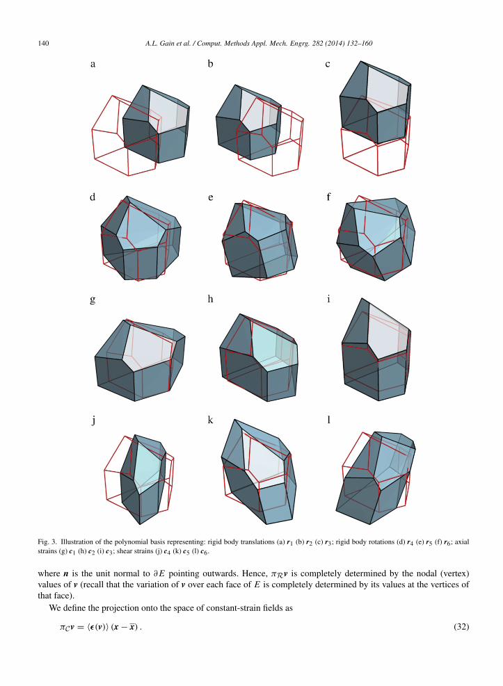
Fig. 3. Illustration of the polynomial basis representing: rigid body translations (a) r1 (b) r2 (c) r3; rigid body rotations (d) r4 (e) r5 (f) r6; axialstrains (g) c1 (h) c2 (i) c3; shear strains (j) c4 (k) c5 (l) c6.

where n is the unit normal to ∂ E pointing outwards. Hence, πRv is completely determined by the nodal (vertex)values of v (recall that the variation of v over each face of E is completely determined by its values at the vertices ofthat face).

We define the projection onto the space of constant-strain fields as

πC v = ⟨ϵ(v)⟩ (x − x) . (32)


One can again directly verify conditions (24) and (26) from this definition. Analogous to (29), we have

πC v = 0, ω(πC v) = 0, ϵ(πC v) = ⟨ϵ(v)⟩ (33)

illustrating the strain associated with πC v is the average of strain of v, and πC v does not contain any rigid bodytranslation or rotation. We can also express the expansion of πC in terms of the basis for C as follows:

πC v = ⟨ϵ(v)⟩(11) c1 + ⟨ϵ(v)⟩(22) c2 + ⟨ϵ(v)⟩(33) c3 + ⟨ϵ(v)⟩(12) c4 + ⟨ϵ(v)⟩(23) c5 + ⟨ϵ(v)⟩(31) c6. (34)

Finally, as with πR, the volume integral in πC v can be written as an integral over the boundary of EE

ϵ(v)dx =12

E

∇v + ∇

⊤v

dx =12

∂ E

(v ⊗ n + n ⊗ v) ds (35)

and so πC v is determined by the nodal values of v.An important property of πC is that for all v ∈ W , the term v − πC v is energetically orthogonal to C, that is

aE (c, v − πC v) = 0, ∀c ∈ C. (36)

As we will see in the next section, this property plays a crucial role in ensuring consistency of the VEM bilinear form.To verify this identity, we appeal to the last equality in (33) and the fact that σ (c) is a constant field:

aE (c, v − πC v) =

E

σ (c) : [ϵ(v) − ϵ(πC v)] dx = σ (c) :

E

ϵ(v)dx − ϵ(πC v) |E |

= 0. (37)

In fact, we can show that (32) is the only projection onto C that satisfies (36). In other words, the energy orthogonalitycondition uniquely determines the projection on C.4

We can also show that this energy orthogonality extends to P and πP . In particular,

aE (p, v − πP v) = 0, ∀p ∈ P (38)

for all v ∈ W . To see this, note that p = πP p and we thus have the following expansion:

aE (p, v − πP v) = aE (πRp, v − πP v) + aE (πC p, v − πC v) − aE (πC p, πRv). (39)

The first and last term on the right hand side vanish since rigid body motions πRp and πRv have zero strain. We notethat (38) is in fact taken as the definition of the projection map πP in the VEM literature [21]. We refer to Section 8of [24] for an alternative approach for defining πP based on this energy orthogonality condition.

With the projection maps defined explicitly, we can obtain an additive kinematic decomposition of a givendeformation state v ∈ W into its rigid body motion, constant strain and the remaining higher-order components:

v = πRv + πC v + (v − πP v) . (40)

The remainder v − πP v belongs to a (3n − 12)-dimensional subspace of W , which we shall denote by H. This spaceconsists of displacement modes that are either higher-order polynomials or non-polynomial functions. For example, ifE is a cube, and W is the space of trilinear displacement fields, v−πP v is a linear combination of 12 hourglass modesconsisting of high-order polynomials. For a distorted hexahedron, these modes will consist of rational functions evenwith the classical iso-parametric finite element bases [34]. For a general polyhedron with 24 vertices, we would have3 × 24 − 12 = 60 modes involving higher-order or non-polynomial deformations.

3.2. Construction of the discrete bilinear forms

The kinematic decomposition of deformation state v in the form (40), by the virtue of energy-orthogonalitycondition (36), leads to a decomposition of strain energy associated with v:

aE (v, v) = aE (πRv + πC v + (v − πP v) , πRv + πC v + (v − πP v))

4 Observe, for instance, that (36) immediately implies (26): for all r ∈ R, we have aE (πC r, πC r) = aE (r, πC r) = 0, the later equality followingfrom ϵ(r) = 0. Since πC r = BS (x − x) for some symmetric matrix BS and aE (πC r, πC r) = |E | CBS : BS, we can conclude that BS = 0 andthus πC r = 0.


= aE (πC v, πC v) + 2aE (πC v, v − πP v) + aE (v − πP v, v − πP v)

= aE (πC v, πC v) + aE (v − πP v, v − πP v). (41)

In the first equality, we have used the linearity and symmetry of aE along with the fact that ϵ(πRv) = 0. The identity(38) and πC v ∈ P , are used in the second equality to eliminate the coupling term. The first term on the right handside of the final expression in (41) represents the energy associated with the constant-strain component of v whilethe second term gives the energy associated with the remaining higher-order part. Observe that the first term can becomputed exactly with the knowledge of the volume of E since its integrand, σ (πC v) : ϵ(πC v), is a constant field.

Now comes another key observation made in [21]: we can replace the second term in (41) by a crude estimate, onethat can be conveniently computed, without affecting the energy associated with rigid body motion and constant-straincomponent of v. This suggests defining the following discrete energy form for E :

aEh (u, v) .

= aE (πC u, πC v) + s E (u − πP u, v − πP v) (42)

where s E is a prescribed symmetric continuous bilinear form on W .Noting that for h ∈ H,

aEh (h, h) = s E (h, h) (43)

it is evident that s E must be positive definite on the space of higher-order deformations H. Otherwise, non-zerohigher-order deformation modes may be assigned zero strain energy, potentially leading to global zero-energy modesand rank deficiency of the global system. In general, we may not have a guarantee of uniform coercivity of ahwhich is required for establishing estimate (15). A suitable choice of s E thus ensures the stability of the methodby guaranteeing that discrete bilinear form inherits the coercivity of the exact bilinear form. As stated in [21,22],a sufficient condition for stability is that for some positive constants β1 and β2, independent of h and E , we haveβ1aE (h, h) ≤ s E (h, h) ≤ β2aE (h, h) for all h ∈ H. This means that the strain energy associated with higher-order modes, as prescribed by s E , scale uniformly with the exact strain energy. As mentioned before, for hexahedralelements, H is the space of hourglass modes, and so, in light of (43), s E essentially prescribes the “hourglass” stiffness(see, for example, [34]).

By virtue of the decomposition, the choice of s E does not affect the first-order polynomial consistency of aEh .

Indeed, for p ∈ P and v ∈ W , we have

aEh (p, v) = aE (πC p, πC v) + s E (p − πP p, v − πP v)

= aE (πC p, πC v) (since p − πP p = 0)

= aE (πC p, v) (by (36))

= aE (p, v) (since ϵ (πC p) = ϵ (πP p) = ϵ (p)) . (44)

This shows that the discrete bilinear form will exactly capture the strain energy associated with the linear deformationp and its variations. As a result, an element based on (42) will pass the first order patch test. The main consequenceof this is that the error introduced by replacing the exact strain energy with ah , the first term in (15), is O(h). To seethis, we first split up exact and discrete strain energies into the element contributions (cf. (7) and (16)) and use (44) toadd and subtract a piecewise polynomial p:

|a (uh, v) − ah (uh, v)| ≤

E∈Th

aE (uh, v) − aEh (uh, v)

=

E∈Th

aE (uh, v) − aE (p, v) + aEh (p, v) − aE

h (uh, v)

=

E∈Th

aE (uh − p, v) − aEh (uh − p, v)

≤ C

E∈Th

∥uh − p∥1,E ∥v∥1,E (using continuity of aE , aEh )

≤ C

E∈Th

∥u − p∥1,E + ∥uh − u∥1,E

∥v∥1,E (triangle inequality). (45)


Here C is a constant independent of the mesh size. To bound the first term, we can choose p such that p|E =

πP (E)u = u + ⟨∇u⟩ (x − x), which is well-defined given the assumed regularity of u. Since πP (E) preserves firstorder polynomials, by Theorem 3.1.4 of [33], ∥u −πP (E)u∥1,E ≤ C ′h |u|2,E . By the Cauchy–Schwarz inequality, wehave

|a (uh, v) − ah (uh, v)| ≤ CC ′h |u|2,Ω + ∥uh − u∥1,Ω

∥v∥1,Ω . (46)

Recalling that the Galerkin error (12) is O(h), it follows that the energy consistency error is also O(h).Regarding choice of the bilinear form s E , there is quite a bit of freedom in practice since s E can be any

approximation of exact strain energy aE , so long as it respects the stability requirement. On one end of the spectrum,we can define s E through quadrature as

s E (u, v) .= σ (u) : ϵ(v)dx. (47)

Here indicates that the volume integral is evaluated using a suitable quadrature rule. This approach has been pursuedin [12,35] in order to alleviate the burden of numerical quadrature in the finite element setting. A simple choice on theother end is given by [21]:

s E (u, v) =

ni=1

αE u(xi ) · v(xi ). (48)

Note that this choice of s E is not a good approximation to the exact strain energy on all of W . For example, itassigns finite energy to non-zero rigid body motions. However, in light of (42), its use only affects the strain energyof higher-order modes. The positive parameter αE is introduced to ensure the right scaling of energies assigned tothese modes. We defer the discussion of determining an appropriate value of this constant to the next section. Observethat this definition only involves the nodal values of the arguments and therefore eliminates the need for volumetricquadrature and construction of the basis functions inside the element. Such a choice highlights the advantage of VEMin constructing an inexpensive discretization scheme on arbitrary meshes.

We remark that the flexibility in the choice of s E can be exploited to enhance other characteristics of the resultingmethod (e.g. satisfaction of a discrete maximum principle or improvement of performance of algebraic solvers) asillustrated in [36,37].

3.3. Construction of fh(v)

It is also possible to construct a first-order accurate discrete load linear form fh without the need for basis functionsin the interior of the elements. A general strategy, proposed in [26], makes use of appropriately defined L2-projectionsof basis functions onto first-order polynomials in the interior of the elements and on the mesh faces. Here we follow anapproach closer to that of [22] for the first-order VEM, which utilizes a nodal quadrature scheme over each element totreat the body force term and a nodal quadrature scheme over each face in the traction boundary Γt, denoted henceforthby Fh,t. Such quadrature rules have also been used in the MFD literature (see for example, [9,10]).

For each v ∈ Vh , we set

fh(v) .=

E∈Th

b · vdx +

F∈Fh,t

Ft · vds (49)

with two quadrature schemes defined as follows (cf. Fig. 4(a)). The two-dimensional surface integral over a face Fwith m vertices is approximated by

FT ds .

=

mj=1

wFj T (xF

j ). (50)

Here xF1 , . . . , xF

m denote the location of vertices incident on face F . The weight wFj is the area of quadrilateral formed

by xFj , the midpoint of edges incident on xF

j , and the centroid of F . It is clear thatm

j=1 wFj = |F | so the quadrature


a

b

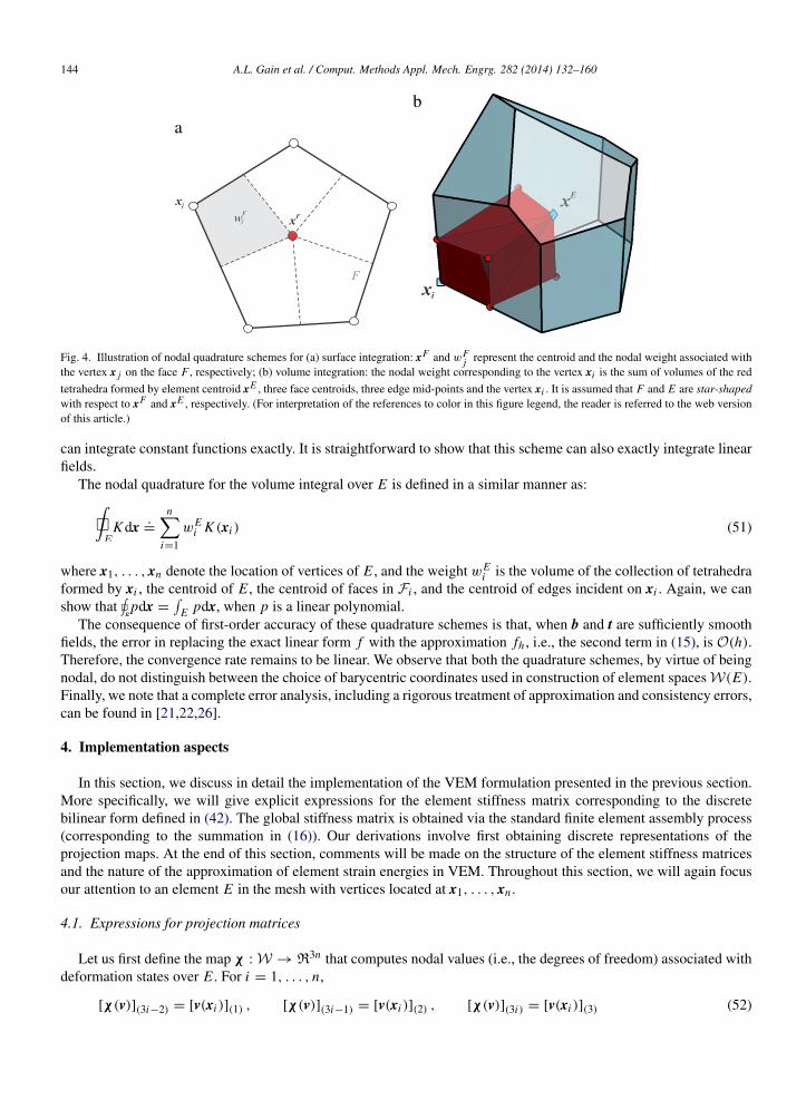
Fig. 4. Illustration of nodal quadrature schemes for (a) surface integration: xF and wFj represent the centroid and the nodal weight associated with

the vertex x j on the face F , respectively; (b) volume integration: the nodal weight corresponding to the vertex xi is the sum of volumes of the red

tetrahedra formed by element centroid xE , three face centroids, three edge mid-points and the vertex xi . It is assumed that F and E are star-shapedwith respect to xF and xE , respectively. (For interpretation of the references to color in this figure legend, the reader is referred to the web versionof this article.)

can integrate constant functions exactly. It is straightforward to show that this scheme can also exactly integrate linearfields.

The nodal quadrature for the volume integral over E is defined in a similar manner as:

K dx .=

ni=1

wEi K (xi ) (51)

where x1, . . . , xn denote the location of vertices of E , and the weight wEi is the volume of the collection of tetrahedra

formed by xi , the centroid of E , the centroid of faces in Fi , and the centroid of edges incident on xi . Again, we canshow that pdx =

E pdx, when p is a linear polynomial.

The consequence of first-order accuracy of these quadrature schemes is that, when b and t are sufficiently smoothfields, the error in replacing the exact linear form f with the approximation fh , i.e., the second term in (15), is O(h).Therefore, the convergence rate remains to be linear. We observe that both the quadrature schemes, by virtue of beingnodal, do not distinguish between the choice of barycentric coordinates used in construction of element spaces W(E).Finally, we note that a complete error analysis, including a rigorous treatment of approximation and consistency errors,can be found in [21,22,26].

4. Implementation aspects

In this section, we discuss in detail the implementation of the VEM formulation presented in the previous section.More specifically, we will give explicit expressions for the element stiffness matrix corresponding to the discretebilinear form defined in (42). The global stiffness matrix is obtained via the standard finite element assembly process(corresponding to the summation in (16)). Our derivations involve first obtaining discrete representations of theprojection maps. At the end of this section, comments will be made on the structure of the element stiffness matricesand the nature of the approximation of element strain energies in VEM. Throughout this section, we will again focusour attention to an element E in the mesh with vertices located at x1, . . . , xn .

4.1. Expressions for projection matrices

Let us first define the map χ : W → R3n that computes nodal values (i.e., the degrees of freedom) associated withdeformation states over E . For i = 1, . . . , n,

[χ(v)](3i−2) = [v(xi )](1) , [χ(v)](3i−1) = [v(xi )](2) , [χ(v)](3i) = [v(xi )](3) (52)


and thus we have the expansion:

v(x) =

3nj=1

[χ (v)]( j) ϕ j (x). (53)

Note that any v ∈ W can be uniquely identified with χ (v) ∈ R3n , and conversely, any array in R3n identifies with amember of W .

The discrete counterpart to projection maps πR, πC are 3n × 3n matrices PR, PC whose application to the nodalrepresentation of v gives the nodal representation of its projection, that is,

PRχ(v) = χ (πRv) , PC χ(v) = χ (πC v) . (54)

Setting v = ϕ j in the above expressions yields the alternative characterization of these matrices as

πRϕ j =

3nk=1

(PR)(k j) ϕk, πC ϕ j =

3nk=1

(PC )(k j) ϕk . (55)

To obtain an explicit expression for PR, we use (30) to write,

πRϕ j =

6ℓ=1

(WR)( jℓ) rℓ. (56)

Here, WR is the 3n × 6 matrix whose j th row is given byϕ j(1)

,ϕ j(2)

,ϕ j(3)

,ω(ϕ j )

(12)

,ω(ϕ j )

(23)

,ω(ϕ j )

(31)

. (57)

Expanding rℓ in terms of the canonical basis functions, ϕk , we obtain,

πRϕ j =

6ℓ=1

(WR)( jℓ)

3n

k=1

[χ (rℓ)](k) ϕk

=

6ℓ=1

3nk=1

(WR)( jℓ) [χ (rℓ)](k) ϕk . (58)

Let, NR ∈ R3n×6 be the matrix whose (k, ℓ)th entry is [χ (rℓ)](k), then

πRϕ j =

3nk=1

NRW⊤

R

(k j)

ϕk . (59)

Finally, by comparing (59) with (55), we conclude that,

PR = NRW⊤

R. (60)

A similar derivation shows that the projection matrix PC can be expressed as:

PC = NC W⊤

C (61)

where, NC , WC ∈ R3n×6 with (NC )(kℓ) = [χ (cℓ)](k) and the j th row of WC given byϵ(ϕ j )

(11)

,ϵ(ϕ j )

(22)

,ϵ(ϕ j )

(33)

,ϵ(ϕ j )

(12)

,ϵ(ϕ j )

(23)

,ϵ(ϕ j )

(31)

. (62)

Note that the matrices PR, PC are projections onto the range of NR, NC , respectively. We can also verify thatPC PR = PRPC = 0. Using (27) and (54) we can find matrix representation of the projection πP as

PP = PR + PC . (63)

Finally, let us note that the null space of PP corresponds to the nodal representations of elements of H.


4.2. Expressions for the stiffness matrix

Using the projection matrices PR, PC defined in the previous section, we next obtain explicit expressions for thestiffness matrix, KE

h , associated with (42). We haveKE

h

( jk)

= aEh (ϕ j , ϕk) = aE (πC ϕ j , πC ϕk) + s E (ϕ j − πP ϕ j , ϕk − πP ϕk). (64)

To simplify the first term, let us first define the 6 × 6 matrix D whose entries are the normalized strain energiesassociated with uniform deformations, i.e.,

(D)(ℓm) =1

|E |aE (cℓ, cm), ℓ, m = 1, . . . , 6. (65)

Using (22), we find that

D =

C(1111) C(1122) C(1133) 2C(1112) 2C(1123) 2C(1131)

C(2222) C(2233) 2C(2212) 2C(2223) 2C(2231)

C(3333) 2C(3312) 2C(3323) 2C(3331)

4C(1212) 4C(1223) 4C(1231)

symm. 4C(2323) 4C(2331)

4C(3131)

(66)

which shows that D is only a function of the elasticity tensor C and does not depend on the geometry of the elementE . For an isotropic material with Young’s modulus EY and Poisson’s ratio ν, matrix D is given by:

D =EY

(1 + ν) (1 − 2ν)

1 − ν ν ν 0 0 0

ν 1 − ν ν 0 0 0ν ν 1 − ν 0 0 00 0 0 2 (1 − 2ν) 0 00 0 0 0 2 (1 − 2ν) 00 0 0 0 0 2 (1 − 2ν)

. (67)

Using the expansion for πC ϕ j similar to (56), we obtain the expression for the first term of the stiffness matrix as

aE (πC ϕ j , πC ϕk) = aE 6

ℓ=1

(WC )( jℓ) cℓ,

6m=1

(WC )(km) cm

=

6ℓ=1

6ℓ=1

(WC )( jℓ)

aE (cℓ, cm)

(WC )(km)

= |E |

WC DW⊤

C

( jk)

. (68)

As for the second term, we first define the 3n × 3n matrix SE whose ( j, k)th entry is s E (ϕ j , ϕk). For example, for thechoice of s E given by (48), we have SE

= αE I3n . Noting that

ϕ j − πP ϕ j =

3nk=1

(I − PP )(k j) ϕk (69)

we can write

s E (ϕ j − πP ϕ j , ϕk − πP ϕk) =

(I − PP )⊤ SE (I − PP )

( jk)

(70)

and so the stiffness matrix is given by

KEh = |E | WC DW⊤

C + (I − PP )⊤ SE (I − PP ) . (71)


As seen from the above expression, the task of computing the stiffness matrix reduces to computing four matricesNR, NC , WR, and WC . We next further break down these calculations and comment on the computational effortneeded for the method.

4.3. Calculation of matrices NR, NC , WR, and WC

Let us first concentrate on the matrices NR and NC which are essentially the nodal representations of the bases ofR and C, respectively. Referring to (21), we can see that, for i = 1, . . . , n, the block of 3i − 2 to 3i rows of NR,which are associated with the i th vertex of the element, is given by:1 0 0 (xi − x)(2) 0 − (xi − x)(3)

0 1 0 − (xi − x)(1) (xi − x)(3) 00 0 1 0 − (xi − x)(2) (xi − x)(1)

. (72)

Similarly, the block 3i − 2 to 3i rows of NC can be expressed as:(xi − x)(1) 0 0 (xi − x)(2) 0 (xi − x)(3)

0 (xi − x)(2) 0 (xi − x)(1) (xi − x)(3) 00 0 (xi − x)(3) 0 (xi − x)(2) (xi − x)(1)

(73)

To facilitate the description of the block of WR and WC associated with the i th vertex, we first define the vector qias:

qi =1

2 |E |

∂ E

ϕi nds. (74)

Recall that ϕi is the scalar barycentric coordinate based on which the element basis functions are defined (cf., (9)).Since ϕi vanishes on F c

i , we have

qi =1

2 |E |

F∈Fi

F

ϕi ds

nF,E (75)

where nF,E is the normal to the face F pointing outwards with respect to element E . Using (9), the definition of WRin (57), and the identity (31), we find the block of 3i − 2 to 3i rows of WR to be1/n 0 0 (qi )(2) 0 − (qi )(3)

0 1/n 0 − (qi )(1) (qi )(3) 00 0 1/n 0 − (qi )(2) (qi )(1)

. (76)

A similar approach can be used to identify the block of 3i − 2 to 3i rows of WC as2 (qi )(1) 0 0 (qi )(2) 0 (qi )(3)

0 2 (qi )(2) 0 (qi )(1) (qi )(3) 00 0 2 (qi )(3) 0 (qi )(2) (qi )(1)

. (77)

The calculation of the matrices WR and WC thus boils down to computation of the surface integrals

F ϕi ds as wellthe unit normal vectors for each face in the mesh. Two additional data structures for Th , beyond the usual vertexlist and vertex-element connectivity matrix, are needed to facilitate these calculations. The first contains the list offaces in the mesh along with vertices incident on each face. The orientation of each face F , and subsequently itsunit normal vector nF , is chosen and fixed once and for all. The second data structure contains the element-faceconnectivity information as well as the orientation of the outer normal nF,E associated with element E . Note thateither nF,E = nF or nF,E = −nF , depending on the initial choice of nF . We should point out that the constructionof these data structures directly from the standard vertex-element connectivity and vertex list, is possible if the meshconsists of convex polyhedra. For example, the faces of an element can be determined by identifying the groups ofvertices that lie on the same plane. Moreover, each internal face of such a mesh is shared exactly between two elements.This insight can be used to identify the internal faces through an inspection of the vertex-element connectivity matrix.


Regarding the surface integrals

F ϕi ds, if boundary barycentric coordinates of [26] are used in the constructionof W(E), the value of this surface integral can be computed exactly from the geometry of F (see the Appendix). Ingeneral, we can use the nodal quadrature scheme presented in Section 3.2 to compute a first-order approximation. Notethat the nodal quadrature does not distinguish between the choice of basis functions and thus the value of the surfaceintegral is purely a function of the geometry of F .5 Such an approximation in fact amounts to using the followingprojection maps

πRv = v +

1

2 |E |

F∈F E

F(v ⊗ n − n ⊗ v) ds

(x − x) (78)

πC v =

1

2 |E |

F∈F E

F(v ⊗ n + n ⊗ v) ds

(x − x) (79)

in (42). Observe that it is necessary for the quadrature rule to exactly integrate linear polynomials in order for thesemaps to respect (23)–(26). We can show that the consistency error in the energy bilinear form (i.e., the first termin (15)) will remain O(h). While the orthogonality conditions (36)–(38), and subsequently (44), are satisfied onlyasymptotically, we will show in Section 5.1 that the global patch test is nevertheless passed exactly.6

4.4. Structure of the stiffness matrix

It is insightful to examine the effects of strain energy approximation in VEM from an algebraic point of viewby considering the structure of the resulting stiffness matrix. Such a perspective is fundamental to the developmentof corresponding MFD formulations that do not directly utilize the existence of underlying basis functions (see, forexample, [9,38]).

To this effect, let us again consider an element E and denote its exact stiffness matrix by KE , i.e., KE( jk) =

aE (ϕ j , ϕk). We assume that the diagonal stability term (48) is used in the definition of the discrete bilinear formand the VEM stiffness KE

h . Complementing the bases for space of rigid body motions and constant strains, we willnext select a basis h1, . . . , h3n−12 for the space of higher-order modes7 H = H(E). This basis will be chosen suchthat the corresponding matrix NH ∈ R3n×(3n−12), i.e., the matrix whose ℓth column is χ (hℓ), satisfies the followingproperties:

N⊤

HNH = I3n−12, N⊤

HKE NH = diag(λE1 , . . . , λE

3n−12). (80)

Observe that λEℓ is the strain energy associated with hℓ, i.e., aE (hℓ, hℓ) = λE

ℓ . To see how such a basis can beselected, we start with matrix NH ∈ R3n×(3n−12) whose columns form an orthonormal basis for the null space ofPP . We choose U to be the orthogonal matrix whose columns are eigenvectors of N⊤

HKE NH and set NH.= NHU.

Since PP NH = PP NHU = 0, the columns of NH indeed correspond to deformation states in H. One can verify thatconditions in (80) hold in this case.

Next, we define a 3n × 3n matrix given by

N = [NR, NC , NH].=χ (r1) , . . . ,χ (r6) , χ (c1) , . . . ,χ (r6) , χ (h1) , . . . ,χ (h3n−12)

(81)

which is invertible since the bases for rigid body motion, uniform and higher-order deformations are linearlyindependent. Owing to the energy-orthogonality of C and H, the exact stiffness matrix form has a block diagonal

5 In fact,F

ϕi ds is simply the area of the quadrilateral formed by the associated vertex xi , the midpoint of edges incident on xi and the centroid

of F .6 Following the same arguments of [26], it is possible to redefine the (virtual) element space W , retaining its polynomial precision, such that the

nodal quadrature and subsequently projection maps (78)–(79) are in fact exact. With that perspective, the first-order consistency condition (44) andthe satisfaction of the global patch test are immediate.

7 Here, we assume that the exact projection maps are available and used to define H.


structure with respect to the basis defined by the columns of N. More specifically, we have

N⊤KE N =

N⊤

RKE NR N⊤

RKE NC N⊤

RKE NH

N⊤

C KE NR N⊤

C KE NC N⊤

C KE NH

N⊤

HKE NR N⊤

HKE NC N⊤

HKE NH

=

0 0 00 |E | D 00 0 diag(λE

1 , . . . , λE3n−12)

. (82)

Similarly, one obtains the following transformation of the VEM stiffness matrix under the same change of basis:

N⊤KEh N =

0 0 00 |E | D 00 0 αE I3n−12

. (83)

Compared to (82), we can see that the only difference lies in the strain energy assigned to the higher-order modesh1, . . . , h3n−12. With the choice of stabilizing bilinear form (48), the energy of these modes is assumed to beidentically equal to αE .

This observation leads us to the question of selection of an appropriate value for the parameter αE . While there area number of possible approaches to addressing this question, we proceed as follows. Because s E can be viewed as anapproximation to the exact strain energy aE , we can compare the energy it assigns to uniform deformations with theirexact energy. Observing that

s E (cℓ, cm) =

N⊤

C SE NC

(ℓm)= αE

N⊤

C NC

(ℓm)(84)

and aE (cℓ, cm) = |E | D(ℓm), the scaling coefficient can be chosen such that αE N⊤

C NC and |E | D are comparable.Equating the trace of this matrix suggests the following relation for the scaling parameter

αE= γαE

⋆ (85)

where

αE⋆

.=

|E | trace (D)

traceN⊤

C NC . (86)

The coefficient γ , taken to be independent of E , is introduced here in order to facilitate the study of the influenceof αE on the accuracy of the numerical solutions. As expected, this expression depends on the material properties,through the trace of D, and the geometry of E through the appearance of NC .

The above argument indicates that a reasonable value for γ should be close to one. In order to validate this assertion,we have computed the strain energy associated with basis for H, i.e., λE

1 , . . . , λE3n−12, of a few representative polyhedra

shown in Fig. 5. The exact stiffness matrix here is computed, by means of a very high order quadrature scheme, for anelement space W(E) defined using maximum entropy basis functions.8 The spectrum is normalized by αE

⋆ in order tofacilitate the comparison with coefficient γ . We can see that the spectrum (cf. Fig. 6) can be relatively broad especiallyfor the irregularly-shaped distorted polyhedra with small edges. However, the average value of the normalized energiesis O(1) for the element geometries considered here. The histogram in Fig. 7 shows the distribution of this average

8 In the case of cube, the underlying space W coincides with the usual finite element space of trilinear functions.


Fig. 5. Representative polyhedra for the study of energy of higher-order modes λEℓ

. (a) Uniform hexahedron. (b) Distorted hexahedron. (c)Polyhedron with 12 vertices. (d) Polyhedron with 24 vertices. Red circles highlight small edges.

Fig. 6. Distribution of normalized strain energies associated with higher-order modes, λEℓ

/αE⋆ , for the polyhedra shown in Fig. 5. The red square

box within each spectrum indicates the average value. (For interpretation of the references to color in this figure legend, the reader is referred to theweb version of this article.)

value for the elements in a centroidal Voronoi mesh with 100 polyhedral elements. We can see a significant clusteringaround 1 confirming that (85) with γ = 1 is a reasonable choice for the strain energy of higher order modes.

5. Numerical studies

In this section, we evaluate the performance of polyhedral discretizations using VEM through several numericalstudies. The accuracy and convergence of the numerical solutions are assessed using two measures of error incomputed displacement and stress fields. The relative error in displacements is defined using the volumetric nodal


Fig. 7. Frequency distribution of the average normalized strain energy3n−12

ℓ=1 λEℓ

/(αE⋆ (3n − 12)) for a Centroidal Voronoi mesh consisting of

100 polyhedral elements.

quadrature rule of Section 3 as:

eu.=

E∈Th

|u − uh |2 dx

E∈Th

|u|2 dx

1/2

. (87)

Recall that uh is the VEM solution and u is the exact solution, assumed to be sufficiently smooth for the quadrature tomake sense. Note that eu serves as an approximation to the L2-norm error ∥u − uh∥0,Ω , which cannot be computedwithout access to the basis functions.

Similarly, we define a discrete error measure for the stress field since the raw field σ (uh) is not readily available.Motivated by the fact that ϵ(πC(E)v) is the volume average of ϵ(v) over element E (cf. (33)) and therefore its bestconstant approximation, we define a element-wise constant stress field on Th , denoted by σ h(v), such that9

σ h(v)|E =1

|E |

E

σ (v)dx = σ (πC v). (88)

This will serve as a surrogate to σ (v) and, accordingly, the following measure of error is considered

eσ.=

∥σ (u) − σ h(uh)∥0,Ω

∥σ (u)∥0,Ω. (89)

We evaluate these integrals numerically with a high-order quadrature obtained as follows: each polyhedral elementis divided into pyramids and a fourth-order Gauss rule consisting of 64 integration points is used over each pyramid(cf. [39]).

We use the open source MATLAB toolbox, Multi-Parametric Toolbox (MPT) [40], for generating the polyhedralmeshes. Two types of polyhedral meshes based on Voronoi tessellations are used in our study: random Voronoi meshes(abbreviated by RND), which are formed by a random set of generating seeds; and more uniform centroidal Voronoitessellations (abbreviated by CVT) that are obtained from a set of seeds that coincide with centroids of the resultingVoronoi cells. The CVT meshes are generated using Lloyd’s algorithm following the approach outlined in [41]. Bothtypes of meshes consist only of convex polyhedra. Finally, in all the numerical results presented here, the local discretebilinear forms are based on choice of s E in (48) with αE given by (85).

9 For each E ∈ Th , we can express this element stress as σ h(v)|E =6

ℓ=1[W⊤

C χ (v)]ℓσ (cℓ).


Fig. 8. Illustration of the displacement patch test with exact solution p = [2x1 + x2 + 3x3 + 1, 3x1 + 4x2 + 2x3 + 2, 4x1 + 3x2 + x3 + 3]⊤/100

(a) CVT mesh, (b) RND mesh, and (c) polyhedral mesh containing non-convex elements. The red box represents Ω and the mesh illustrates thedeformed configuration. (For interpretation of the references to color in this figure legend, the reader is referred to the web version of this article.)

5.1. Displacement patch test

We start with the displacement patch test on the unit cube Ω = (0, 1)3 discretized using CVT and RND mesheswith different number of polyhedrons. We have also considered meshes containing non-convex elements. The exactsolution for the patch test is an arbitrary linear displacement field u = p ∈ P(Ω). We consider the case where Γt = ∅

and g = p|∂Ω is applied to the entire boundary (note that the body forces are absent, i.e., b = 0). Fig. 8 shows thedeformed configuration of the three representative meshes tested. The relative displacement and stress errors close tomachine precision levels, for a large range of γ values, are observed for CVT meshes indicating that VEM passesdisplacement patch test. For random Voronoi meshes the errors are approximately one order of magnitude higher thanCVT mesh errors but still close to machine precision levels.

These results are consistent with the theoretical discussion thus far when the projection maps are computed exactly(e.g., when the element space is obtained using boundary coordinates of [26]). However, we have also observed thesatisfaction of the global patch test even when nodal quadrature is used in the definition of the projection maps (cf.(78) and (79)). In this case, the element level condition of exactness of strain energy, i.e., (44), may not be satisfiedexactly. Nevertheless we can prove directly that the global patch test should be passed. First note that, for p ∈ P(E)

and v ∈ W(E), and using projection maps obtained from nodal quadrature, we have

aEh (p, v) = aE (p, πC v)

= σ (p) :

E

ϵ(πC v)dx

= σ (p) :

F∈F E

12 F

(v ⊗ n + n ⊗ v) ds

=

F∈F E

Fv · σ (p)nds (using symmetry of σ (p)). (90)

Now, let us consider a general patch test with exact solution u = p ∈ P(Ω). Corresponding tractions t = σ (p)n areimposed on Γt, and g = p|Γu is applied to the remainder of the boundary. For an arbitrary test function v ∈ V 0

h , wesee that

ah (p, v) =

E∈Th

aEh (p, v) =

E∈Th

F∈F E

Fv · σ (p)nds =

F∈Fh,t

Fv · tds = fh(v). (91)

In the second to last equality, we have used the fact that boundary integrals on the internal faces cancel out and v = 0on Γu. Since p ∈ V g

h , this shows that uh = p is the unique solution to the discrete problem and the global patch test ispassed.


Table 1Comparison between maximum entropy finite element and VEM for displacement patch test. The second and third columns show the relativedisplacement errors eu.

Number of elements Maximum entropy VEM

50 8.14 × 10−2 5.72 × 10−15

100 9.24 × 10−2 1.91 × 10−14

200 6.63 × 10−2 2.66 × 10−14

For the sake of comparison, we repeat the patch test using a finite element method based on the conformingmaximum entropy basis functions [42] and numerical integration of the stiffness matrix. The errors in the patch testperformed for a sequence of meshes is indicative of the consistency error introduced by the quadrature in the elementaland global strain energies. Numerical integration is carried out by first partitioning each element into tetrahedra usingthe element center, face centers and vertex locations and using standard quadrature rules on each tetrahedron. On aCVT mesh of 50 elements, the observed relative errors in displacement are 1.84×10−1, 8.14×10−2 and 4.93×10−2

when first, second and fourth order quadrature rules (consisting of 1, 4 and 11 points) are used for each tetrahedron.Table 1 shows the errors for a sequence of CVT meshes with the second order rule indicating that the errors persistunder mesh refinement. As discussed in detail in [12], the failure to satisfy patch test, at least asymptotically undermesh refinement, can place a limit on the accuracy that can be achieved in general by the method.

5.2. Beam under shear

Next, we study the performance of VEM for a cantilever beam loaded in shear. The domain Ω for this problemis (−1, 1) × (−1, 1) × (0, L), which is occupied by an isotropic material with Young’s modulus EY and Poisson’sratio ν, and is subjected to constant tractions, given by t = [0, −F, 0]⊤, on the face passing through the origin. Theexpressions for stresses are available in [43] and repeated here for completeness:

σ (11) = σ (22) = σ (12) = 0, σ (33) =3F

4x(2)x(3)

σ (31) =3Fν

2π2 (1 + ν)

∞n=1

(−1)n

n2 cosh (nπ)sinnπx(1)

sinh

nπx(2)

(92)

σ (23) =

3F

1 − x2(2)

8

+

Fν

3x2(1) − 1

8 (1 + ν)

−3Fν

2π2 (1 + ν)

∞n=1

(−1)n

n2 cosh (nπ)cos

nπx(1)

cosh

nπx(2)

.

The displacement fields corresponding to these stresses, up to the addition of a rigid body motion, is given by

u(1) = −3Fν

4EYx(1)x(2)x(3)

u(2) =F

8EY

3νx(3)

x2(1) − x2

(2)

− x3

(3)

(93)

u(3) =F

8EY

3x(2)x2

(3) + νx(2)

x2(2) − 3x2

(1)

+

2 (1 + ν)

EYz(x)

where z(x) is the anti-derivative of σ (23) with respect to x(2). In the present numerical study, the length of the beamis L = 10, the shear load is taken as F = 0.1, and the material properties are selected as EY = 25 and ν = 0.3.Moreover, Γu is taken to be the face passing through x(3) = L and boundary displacements are set to g = u|Γu .In addition to CVT and RND meshes, we also consider uniform meshes of hexahedral (brick) elements. This alsoallows for a direct comparison with standard trilinear finite elements on hexahedra. As a means to visualize the beamdeformation and the stress field generated under the shear load, we show representative results in Fig. 9 for CVT andRND meshes.

In our numerical studies, we have observed that the use of boundary coordinates of [26] with the known surfaceintegrals yields almost identical solutions (less than 0.2% and 0.4% difference in the errors for CVT and RND


Fig. 9. Deformation plots for the beam under shear for (a) CVT and (b) RND meshes, and beam experiencing torsion for (c) CVT and (d) RNDmeshes. The colors indicate the magnitude of average von Mises stress.

a b

Fig. 10. Convergence study for VEM under mesh refinement on different meshes, namely CVT Voronoi, random Voronoi (RND) and hexahedralmesh (HEX). (a) Displacement errors, eu. (b) Stress errors, eσ . Results pertaining to polyhedral meshes are average of 5 meshes.

meshes, respectively) to those obtained from the application of nodal quadrature for computing the projection maps.Subsequently, we will only present results using the nodal quadrature in the remainder of this section.

First, we verify the convergence of the VEM under refinement for different mesh types. The results of this studyare shown in Fig. 10 where the relative errors are plotted against the average element diameters. Here the scalingcoefficient is set to αE

= αE⋆ corresponding to γ = 1. For CVT and RND meshes, each point in the curve represents

the average values of a set of five meshes with the same number of elements. As evident from the plots, we havesecond-order convergence in displacements and first-order convergence in stresses in all cases. The fact that theseoptimal convergence rates are observed for RND meshes with many irregular elements is encouraging and a testamentto the robustness of the method.

As a way of comparing the performance of the VEM for the different mesh type, we next plot the error as a functionof total number of degrees of freedom (DoFs) in Fig. 11. For the displacement fields, the CVT and RND meshes


a b

Fig. 11. Plot of the VEM error versus total number of degrees of freedom (DoFs) for CVT, RND, and HEX meshes. The error for the trilinear finiteelement on the hexahedral meshes is labeled HEX FEM. The results for all five CVT and RND meshes are shown. (a) Displacement errors, eu. (b)Stress errors, eσ .

a b

Fig. 12. Study of the optimal scaling coefficient γ for the shear-loaded beam problem for different meshes. (a) Displacement errors, eu. (b) Stresserrors, eσ . Each point of the CVT and RND curves represents the average errors of 5 meshes. The smallest value of γ used here is 0.01.

produce similar errors, while the hexahedral meshes are marginally more accurate. The same trend is observed for theerrors in the stress field though the difference between the mesh types is more pronounced. We also note that there islittle variability in the accuracy of each set of polyhedral meshes, even for the coarsest random Voronoi partitions.

While the preceding theoretical discussion illustrates that optimal convergence of the solutions can be expectedwith any fixed value of γ for sufficiently regular meshes, the choice of γ can play a significant role in the accuracy ofsolutions. In order to study this effect, we next perform a parametric study and plot errors for the shear-loaded beamas a function of γ for each mesh type (see Fig. 12). The results for CVT and RND meshes are the average of fivemeshes with 200 elements. The hexahedral mesh has 625 elements but comparable number of degrees of freedomto the polyhedral meshes. As a point of reference, the errors produced by classical trilinear finite elements on thishexahedral mesh are also indicated on the plots.

A few observations regarding these results are in order. First, as seen in Fig. 12(a), there exists an optimal value of γ

for each mesh type where the displacement errors are minimized. The solutions can be significantly more accurate forthis value of γ . For example, the VEM solution on the hexahedral mesh has almost two orders of magnitude smallererror compared to the corresponding finite element solution. We also note that the sensitivity of the error is larger forγ values less than this optimal value. Conversely, there is less variation in errors for larger values of γ across meshtypes.


Fig. 13. Illustration of optimum γ for the shear-loaded beam problem under refinement for CVT, RND, and HEX meshes.

In contrast to the displacement errors, the stress errors are far less sensitive to the change in γ and almost constantin the range considered here. This could be partially attributed to the fact that the influence of higher-order modes donot show up in this measure of error. We also note that the VEM error levels on the hexahedral mesh are comparableto the finite element errors.

In a final study of the shear problem, summarized in Fig. 13, we study the effects of mesh refinement on theoptimal value of the scaling coefficient. Here the optimal value of γ , with respect to eu, are determined and plottedfor different meshes at different levels of refinement. Aside from a mild increase for the CVT meshes on average,the optimal γ is fairly stable under mesh refinement. It may be possible to exploit this fact in practice and use coarsemeshes to estimate an optimal range for the scaling coefficient for the problem at hand, subsequently used for a morerefined analysis.

5.3. Beam under torsion

We conclude this section by repeating similar numerical studies considering deformation of the same beam undertorsion. The analytical stress field for this problem is given by [43]

σ (11) = σ (22) = σ (33) = σ (12) = 0,

σ (31) =8EYβ

π2 (1 + ν)

∞n=1

(−1)n

(2n − 1)2 cosh [(2n − 1) π/2]cos

(2n − 1) πx(1)/2

sinh

(2n − 1) πx(2)/2

(94)

σ (23) =EYβ

2 (1 + ν)

2x(1) +

∞n=1

16(−1)n

π2 (2n − 1)2 cosh [(2n − 1) π/2]

× sin(2n−1) πx(1)/2

cosh

(2n−1) πx(2)/2

and displacements, up to rigid body motion, by

u(1) = −βx(2)x(3)

u(2) = βx(3)x(1) (95)

u(3) =β

x(1)x(2) +

∞n=1

32(−1)n

π3 (2n − 1)3 cosh [(2n − 1) π/2]sin(2n−1) πx(1)/2

sinh

(2n−1) πx(2)/2

.

Here z(x) is the anti-derivative of σ (23) with respect to x(2) and β is the twist per unit length which is proportional tothe applied torque. For the numerical results here, we choose β = 0.1 and applied displacement boundary conditionsto faces at x(3) = 0 and x(3) = L . The beam deformation and the stress field generated under the torsional load fortwo representative meshes are shown in Fig. 9.


a b

Fig. 14. Plot of error versus total number of degrees of freedom (DoFs) for CVT, RND, and HEX meshes for beam under torsion problem. Theerror for the trilinear finite element on the hexahedral meshes are labeled HEX FEM. (a) Displacement errors, eu. (b) Stress errors, eσ .

a b

Fig. 15. Study of the optimal scaling coefficient γ for the torsion-loaded beam problem for different meshes. (a) Displacement errors, eu. (b) Stresserrors, eσ . Each point of the CVT and RND curves represents the average errors of 5 meshes.

In Fig. 14, we have plotted the errors as a function of the total number of DoFs for the same set of meshes andγ = 1. We can observe similar trends and convergence behavior of VEM as in the shear problem.

Next, we perform a parametric study for γ for each mesh type (see Fig. 15). As before, the results for CVT andRND meshes are the average of five meshes with 200 elements. The optimal value of γ for all meshes again fallsin the range of 0–1, though its influence on the displacement error is far less pronounced for the polyhedral meshescompared to the shear problem. We stress, however, that the optimal value of γ observed in these studies is particular tothe problems considered here and one cannot make generalizations for other problems. For example, additional studieson the appropriate choice of the stabilization term are needed for problems involving highly anisotropic materials withan appropriate balance of simplicity, efficiency and accuracy. Motivated by element-level energetic considerations ofSection 4.4, we recommend using γ = 1 for general polyhedral meshes in the absence of additional insights into thenature of the problem at hand.

6. Concluding remarks

In this work, we discussed the theoretical and practical aspects of VEM in the context of three-dimensionalelasticity problems on polyhedral meshes. At the core of the method, local polynomial projections are used to


decompose the element strain energy into its uniform strain and higher-order components. When constructing anapproximate (discrete) strain energy for an element, preserving the former guarantees the satisfaction of the patchtest and the consistency of the method. One can ensure first-order convergence with a suitable but possibly crudeapproximation of the energy of higher-order modes. As discussed in [12], this splitting of energy can be useful forrestoring consistency for polyhedral finite elements in the presence of quadrature error in the evaluation of strainenergy. As such, the core concepts underlying VEM can provide an alternative approach for addressing the challengesfacing finite element schemes on arbitrary grids. Finally, the extension of VEM in its full generality to nonlinearelasticity problems, though not immediately obvious, is of significant interest. In this regard, we note the recent workon extending MFD and corresponding VEM schemes to quasilinear elliptic problems [44,45].

Acknowledgments

We are thankful to the support from the US National Science Foundation under grant numbers 1321661 and1437535, and from the Donald B. and Elizabeth M. Willett endowment at the University of Illinois at Urbana-Champaign. We also acknowledge partial support provided by Tecgraf/PUC-Rio (Group of Technology in ComputerGraphics), Rio de Janeiro, Brazil. Any opinion, finding, conclusions or recommendations expressed here are those ofthe authors and do not necessarily reflect the views of the sponsors or sponsoring agencies. We acknowledge Prof.Anton Evgrafov for suggesting, during the World Congress of Computational Mechanics (WCCM 2012, Brazil), thatwe investigate the class of mimetic numerical methods in order to develop our polygonal discretization scheme in threedimensions—his suggestion was the inception of the work in the present paper. We would also like to acknowledgethe anonymous reviewers for their insightful comments which helped to improve the present work.

Appendix

In the recent work by Ahmed et al. [26], a particular set of barycentric coordinates on polygons are constructedsuch that their first-order moments can be computed exactly. We will now briefly discuss these coordinates, which isused in the construction of local element space W(E).

Consider a polygon F ⊆ R2 with m vertices located in counter-clockwise order at xF1 , . . . , xF

m . The barycentriccoordinate ϕi associated with i th vertex is equal to one at xi , decays linearly along the incident edges and vanishesat other vertices of F . In the interior of the polygon, ϕi is a function whose Laplacian is a linear field subject to thecondition that its zeroth and first moments equal the corresponding moments of its polynomial projection pi definedby

pi.=

1m

+

1

|F |

∂ F

ϕi nds

·

x − xF

. (96)

Here, n is the unit normal to the boundary of F and xF=

1m

mj=1 xF

j . Denoting by ni the unit normal to the edgeconnecting the (i − 1) and i th vertices, we can simplify the expression for pi as

pi =1m

+1

2 |F |

xFi − xF

i−1

ni +

xFi+1 − xF

i

ni+1

·

x − xF

. (97)

Since there is a one-to one mapping between the moments of these functions and their Laplacian, the condition that ϕiand pi have identical first-order moments uniquely defines the coordinates ϕi . Note that we will not need to computethese coordinates explicitly in the interior of faces in VEM since we only need the average value. This quantity, byconstruction, can be computed as

Fϕi dx =

F

pi dx =|F |

m+

12

xFi − xF

i−1

ni +

xFi+1 − xF

i

ni+1

·

xF

− xF

(98)

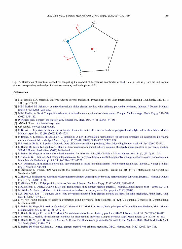
where xF is the centroid of F (cf. Fig. 16).


Fig. 16. Illustration of quantities needed for computing the moment of barycentric coordinates of [26]. Here, ni and ni+1 are the unit normalvectors corresponding to the edges incident on vertex xi and in the plane of F .

References

[1] M.S. Ebeida, S.A. Mitchell, Uniform random Voronoi meshes, in: Proceedings of the 20th International Meshing Roundtable, IMR 2011,2011, pp. 273–290.

[2] M.M. Rashid, M. Selimotic, A three-dimensional finite element method with arbitrary polyhedral elements, Internat. J. Numer. MethodsEngrg. 67 (2) (2006) 226–252.

[3] M.M. Rashid, A. Sadri, The partitioned element method in computational solid mechanics, Comput. Methods Appl. Mech. Engrg. 237–240(2012) 152–165.

[4] P. Dvorak, New element lops time off CFD simulations, Mach. Des. 78 (5) (2006) 154–155.[5] ANSYS Fluent. http://www.ansys.com.[6] CD-adapco. www.cd-adapco.com.[7] F. Brezzi, K. Lipnikov, V. Simoncini, A family of mimetic finite difference methods on polygonal and polyhedral meshes, Math. Models

Methods Appl. Sci. 15 (10) (2005) 1533–1551.[8] F. Brezzi, K. Lipnikov, M. Shashkov, V. Simoncini, A new discretization methodology for diffusion problems on generalized polyhedral

meshes, Comput. Methods Appl. Mech. Engrg. 196 (37–40) (2007) 3682–3692. SPEC. ISS..[9] F. Brezzi, A. Buffa, K. Lipnikov, Mimetic finite differences for elliptic problems, Math. Modelling Numer. Anal. 43 (2) (2009) 277–295.

[10] L. Beirao Da Veiga, K. Lipnikov, G. Manzini, Error analysis for a mimetic discretization of the steady stokes problem on polyhedral meshes,SIAM J. Numer. Anal. 48 (4) (2010) 1419–1443.

[11] L. Beirao Da Veiga, A mimetic discretization method for linear elasticity, ESAIM Math. Model. Numer. Anal. 44 (2) (2010) 231–250.[12] C. Talischi, G.H. Paulino, Addressing integration error for polygonal finite elements through polynomial projections: a patch test connection,

Math. Models Methods Appl. Sci. 24 (8) (2014) 1701–1727.[13] C.R. Dohrmann, M.M. Rashid, Polynomial approximation of shape function gradients from element geometries, Internat. J. Numer. Methods

Engrg. 53 (2002) 945–958.[14] S. Rjasanow, S. Weißer, FEM with Trefftz trial functions on polyhedral elements, Preprint Nr. 316, FR 6.1-Mathematik, Universitat des

Saarlandes, 2012.[15] J. Bishop, A displacement-based finite element formulation for general polyhedra using harmonic shape functions, Internat. J. Numer. Methods

Engrg. 97 (1) (2014) 1–31.[16] P. Milbradt, T. Pick, Polytope finite elements, Internat. J. Numer. Methods Engrg. 73 (12) (2008) 1811–1835.[17] S.R. Idelsohn, E. Onate, N. Calvo, F. Del Pin, The meshless finite element method, Internat. J. Numer. Methods Engrg. 58 (6) (2003) 893–912.[18] M. Wicke, M. Botsch, M. Gross, A finite element method on convex polyhedra, Eurographics 23 (3) (2007).[19] K.Y. Dai, G.R. Liu, T.T. Nguyen, An n-sided polygonal smoothed finite element method (nSFEM) for solid mechanics, Finite Elem. Anal.

Des. 43 (2007) 847–860.[20] S.W. Key, Rapid meshing of complex geometries using polyhedral finite elements, in: 12th US National Congress on Computational

Mechanics, 2013.[21] L. Beirao Da Veiga, F. Brezzi, A. Cangiani, G. Manzini, L.D. Marini, A. Russo, Basic principles of Virtual Element Methods, Math. Models

Methods Appl. Sci. 23 (1) (2013) 199–214.[22] L. Beirao Da Veiga, F. Brezzi, L.D. Marini, Virtual elements for linear elasticity problems, SIAM J. Numer. Anal. 51 (2) (2013) 794–812.[23] F. Brezzi, L.D. Marini, Virtual Element Methods for plate bending problems, Comput. Methods Appl. Mech. Engrg. 253 (2013) 455–462.[24] L. Beirao Da Veiga, F. Brezzi, L.D. Marini, A. Russo, The Hitchhiker’s guide to the Virtual Element Method, Math. Models Methods Appl.

Sci. 24 (8) (2014) 1541–1573.[25] L. Beirao Da Veiga, G. Manzini, A virtual element method with arbitrary regularity, IMA J. Numer. Anal. 34 (2) (2013) 759–781.

http://refhub.elsevier.com/S0045-7825(14)00150-9/sbref2



http://www.ansys.com

http://www.cd-adapco.com



















[26] B. Ahmad, A. Alsaedi, F. Brezzi, L.D. Marini, A. Russo, Equivalent projectors for Virtual Element Methods, Comput. Math. Appl. 66 (3)(2013) 376–391.

[27] F. Brezzi, A. Buffa, K. Lipnikov, Mimetic finite differences for elliptic problems, ESAIM Math. Model. Numer. Anal. 43 (2) (2009) 277–295.[28] G. Strang, G. Fix, An Analysis of the Finite Element Method, second ed., Wellesley-Cambridge, 2008.[29] R. Sibson, A vector identity for the Dirichlet tessellation, Math. Proc. Cambridge Philos. Soc. 87 (1980) 151–155.[30] V.V. Belikov, V.D. Ivanov, V.K. Kontorovich, S.A. Korytnik, A. Yu. Semenov, The non-Sibsonian interpolation: a new method of interpolation

of the values of a function on an arbitrary set of points, Comput. Math. Math. Phys. 37 (1) (1997) 9–15.[31] K. Hormann, N. Sukumar, Maximum entropy coordinates for arbitrary polytopes, in: Eurographics Symposium on Geometry Processing,

vol. 27, 2008, pp. 1513–1520.[32] T. Ju, P. Liepa, J. Warren, A general geometric construction of coordinates in a convex simplicial polytope, Comput. Aided Geom. Design

(ISSN: 0167-8396) 24 (3) (2007) 161–178.[33] P.G. Ciarlet, The Finite Element Method for Elliptic Problems, second ed., SIAM, 2002.[34] T.B. Belytschko, W.K. Liu, J.M. Kennedy, Hourglass control in linear and nonlinear problems, Comput. Methods Appl. Mech. Engrg. 43 (3)

(1984) 251–276.[35] G. Manzini, A. Russo, N. Sukumar, New perspectives on polygonal and polyhedral finite element methods, Math. Models Methods Appl. Sci.

24 (8) (2014) 1665–1699.[36] K. Lipnikov, M-adaptation for numerical solution of PDEs, in: Workshop on Discretization Methods for Polygonal and Polyhedral Meshes,

2012.[37] K. Lipnikov, G. Manzini, M. Shashkov, Mimetic finite difference method, J. Comput. Phys. 257 (2014) 1163–1227.[38] L. Beirao Da Veiga, V. Gyrya, K. Lipnikov, G. Manzini, Mimetic finite difference method for the Stokes problem on polygonal meshes,

J. Comput. Phys. 228 (19) (2009) 7215–7232.[39] D. Sohn, Y.-S. Cho, S. Im, A novel scheme to generate meshes with hexahedral elements and poly-pyramid elements: the carving technique,

Comput. Methods Appl. Mech. Engrg. 201–204 (2012) 208–227.[40] M. Kvasnica, P. Grieder, M. Baotic, Multi-Parametric Toolbox (MPT), 2004. http://control.ee.ethz.ch/˜mpt/.[41] C. Talischi, G.H. Paulino, A. Pereira, I.F.M. Menezes, Polymesher: a general-purpose mesh generator for polygonal elements written in

Matlab, Struct. Multidiscip. Optim. 45 (3) (2012) 309–328.[42] N. Sukumar, Construction of polygonal interpolants: a maximum entropy approach, Internat. J. Numer. Methods Engrg. 61 (12) (2004)

2159–2181.[43] J.R. Barber, Elasticity, third ed., Springer, 2010.[44] P.F. Antonietti, N. Bigoni, M. Verani, Mimetic finite difference approximation of quasilinear elliptic problems, in: Calcoly, 2014,

http://dx.doi.org/10.1007/s10092-014-0107.[45] P.F. Antonietti, L. Beirao Da Veiga, N. Bigoni, M. Verani, Mimetic finite differences for nonlinear and control problems, Math. Models

Methods Appl. Sci. 24 (8) (2014) 1457–1493.













http://control.ee.ethz.ch/~mpt/




http://dx.doi.org/doi:10.1007/s10092-014-0107


on the virtual element method for three-dimensional linear

Documents