on the transmission of monetary policy to the housing market

On the transmission of monetary policy to the housing market Winfried Koeniger, Benedikt Lennartz, Marc-Antoine Ramelet

SNB Working Papers 6/2021

DISCLAIMER The views expressed in this paper are those of the author(s) and do not necessarily represent those of the Swiss National Bank. Working Papers describe research in progress. Their aim is to elicit comments and to further debate. COPYRIGHT© The Swiss National Bank (SNB) respects all third-party rights, in particular rights relating to works protected by copyright (infor-mation or data, wordings and depictions, to the extent that these are of an individual character). SNB publications containing a reference to a copyright (© Swiss National Bank/SNB, Zurich/year, or similar) may, under copyright law, only be used (reproduced, used via the internet, etc.) for non-commercial purposes and provided that the source is menti-oned. Their use for commercial purposes is only permitted with the prior express consent of the SNB. General information and data published without reference to a copyright may be used without mentioning the source. To the extent that the information and data clearly derive from outside sources, the users of such information and data are obliged to respect any existing copyrights and to obtain the right of use from the relevant outside source themselves. LIMITATION OF LIABILITY The SNB accepts no responsibility for any information it provides. Under no circumstances will it accept any liability for losses or damage which may result from the use of such information. This limitation of liability applies, in particular, to the topicality, accuracy, validity and availability of the information. ISSN 1660-7716 (printed version) ISSN 1660-7724 (online version) © 2021 by Swiss National Bank, Börsenstrasse 15, P.O. Box, CH-8022 Zurich

Legal Issues

1

On the Transmission of Monetary Policy to the

Housing Market �

Winfried Koenigera Benedikt Lennartzb

Marc-Antoine Rameletc

February 19, 2021

Abstract

We provide empirical evidence on the heterogeneous transmission of monetary pol-

icy to the housing market across and within countries. We use household-level data

from Germany, Italy and Switzerland together with the respective monetary policy

shocks identified from high-frequency data. We find that the pass-through of mone-

tary policy shocks to rates of newly originated (fixed-rate) mortgages is twice as strong

in Switzerland than in Germany and Italy. After an accommodative monetary policy

shock, this is associated in the housing market with a larger immediate, and persis-

tent increase of transitions from renting to owning; a stronger decrease in rents; and

an increase of the price-rent ratio. Within Italy, we find a stronger pass-through to

mortgage rates, housing tenure transitions and the price-rent ratio in the northern re-

gions that have been characterized in the literature as more financially developed than

the southern regions.

Keywords: Monetary policy transmission, Housingmarket, Home ownership, Rents, House prices.

JEL-codes: E21, E52, R21.

�We thank an anonymous referee, colleagues and participants at seminars and conferences for theirhelpful comments; Oliver Krek for research assistance; and Peter Bolliger for the helpful discussions on theHABE dataset. This paper contains substantially revised results previously circulated with the working title“Home Ownership and Monetary Policy Transmission.” The views, opinions, findings, and conclusions orrecommendations expressed in this paper are strictly those of the author(s). They do not necessarily reflectthe views of the Swiss National Bank (SNB). The SNB takes no responsibility for any errors or omissions in,or for the correctness of, the information contained in this paper.a: University of St.Gallen, CESifo, CFS, IZA; Address: Department of Economics, University of St.Gallen,SEW-HSG, Varnbuelstrasse 14, 9000 St.Gallen, Switzerland, [email protected];b: Department of Economics, University of St.Gallen, SEW-HSG, [email protected];c: Swiss National Bank, [email protected].

1

2

1 Introduction

The transmission of monetary policy is at the core of the research agenda in economics.

Much research has focused on the response of consumption and output to shocks to the

policy rate (Galı, 2015). Recent research by Calza et al. (2013) and Corsetti et al. (2020)

has documented a sizable heterogeneity of monetary policy transmission across euro area

countries, and that this heterogeneity is associated with differences in the housing market.

We contribute to that literature by providing evidence at the household level on the

transmission of monetary policy to the housing market. We focus on Germany, Italy and

Switzerland, which differ in at least two important dimensions: (i) the size of the market

for rental housing and its ownership structure and (ii) the indebtedness of new home-

owners and the characteristics of the mortgage market. We explain in Section 2 that these

dimensions matter for the transmission of policy rate shocks to the homeownership rate

and the price-rent ratio because they affect the pass-through to the rental price of housing

units and the user cost of owning a home.

We estimate the transmission to the housing market using household-level data to-

gether with monetary policy shocks identified from high-frequency data. Our use of

household-level data has the advantage that we can analyze transitions (gross flows) across

housing tenure states of individual households, together with the pass-through of the pol-

icy rate shocks to rents and housing values. Analyzing the differences in the pass-through

across households yields insights on the causes for the heterogeneous transmissions across

countries.

We find that the pass-through of an unexpected change of the policy rate to rates of

newly originated (fixed-rate) mortgage rates is about 80% in Switzerland but only half

that in Germany and Italy. After an unexpected reduction in the policy rate by 25 bp,

transitions from renting to owning a home increased by 1−2 pp in Germany and Switzer-

land but not in Italy, whereas transitions from owning to renting increased by 0.5 pp in

Switzerland but not significantly in the other countries. These effects on the gross flows

for Germany and Switzerland are quantitatively important, as illustrated by considering

a policy rate shock of one standard deviation. Then the effects on the transitions previ-

ously mentioned must be scaled down by approximately one third because the standard

deviation of the monetary policy shocks is 7 bp for the European Central Bank (ECB) and

10 bp for the Swiss National Bank (SNB). The resulting effects on the transitions remain

sizable given that the average rate per year, at which households change housing tenure

from renting to owning for the considered countries, is 4 percent and the average rate per

year, at which households change from owning to renting, is 1− 2 percent.

The implied increase in the net flow toward owning after a policy rate reduction in

Germany and Switzerland is associated with a stronger increase of the price-rent ratio in

2

2

Switzerland than in Germany and Italy. Rents decrease by 3.5 percent in Switzerland but

we do not detect significant decreases in rents for the other two countries. We provide

suggestive evidence that public ownership of rental housing, which is less important in

Switzerland than in Germany and Italy, together with the indexation of rents to mortgage

interest rates in Switzerland, as described further in Section 2, may explain the differentresponse of rents across countries.

We uncover the regional heterogeneity of the pass-through to the mortgage rate withinItaly, which is associated with differences in financial development. We find that an unex-

pected interest rate reduction triggers more transitions to homeownership and a stronger

decrease of rents in more financially developed Italian regions. From a methodological

point of view, the regional heterogeneity within Italy allows for an alternative identifi-

cation of monetary policy transmission to the housing market. Both the results across

countries and across regions within Italy illustrate how differences in the pass-through

to mortgage rates are associated with differences in the transmission to housing tenure

transitions, rents and price-rent ratios.

These results are of interest because monetary policy transmission to quantities and

prices in the housing market matters not only for the housing market itself but also for

the response of aggregate non-housing consumption. The implied distributional effectsacross renters and mortgagors, for example, affect aggregate consumption because these

subgroups of the population differ in their marginal propensity to consume (Cloyne et al.,

2020). Hence, from an applied theoretical perspective, our results provide targets for

the considered countries that help to discipline quantitative models with housing which

attempt to capture these distributional effects, along the lines of recent research, e.g., by

Kaplan et al. (2020), Hedlund et al. (2016), Wong (2019) for the U.S., or Kaas et al. (2021),

Hintermaier and Koeniger (2018) for countries in the euro area.

Monetary policy transmission to rental prices in the housing market also matters for

changes of the consumer price index, a key target of central banks. Indeed, Dias and

Duarte (2019) show for the U.S. that the consumer price responses to monetary policy

shocks are much stronger if the price for shelter is excluded because rents decrease afteran (expansionary) unexpected reduction in the policy rate. Our analysis suggests that this

effect is particularly relevant for Switzerland where rents decrease strongly after policy

rate reductions and the incidence of renting is high, and less so for Germany where public

ownership of rental units seems to mitigate the pass-through of monetary policy shocks

to rents. The latter also applies to Italy where, in addition, the incidence of renting is

much lower than in Germany and Switzerland (see Section 2).

The empirical literature on the transmission of monetary policy to the housing mar-

ket is small compared with the vast literature on consumption responses (Piazzesi and

3

3

4

Schneider, 2016). Beraja et al. (2018) and Wong (2019) focus on the mortgage refinancing

channel for consumption responses which is important for the U.S. where refinancing is

not as costly as in the countries we analyze (see Section 2). We refer to Cloyne et al. (2020)

for a concise overview of the recent literature. Cloyne et al. (2020) estimate heterogeneous

consumption responses across housing tenure groups and show how these responses re-

late to the different balance sheet positions of these groups.1 They do not find an eco-

nomically and statistically significant effect of monetary policy shocks on housing tenure

shares in the U.S. and U.K. (see their online appendix). Fuster and Zafar (2021) find small

effects of changes in financing costs on the willingness to pay for house purchases, based

on a strategic survey in which respondents in the U.S. revealed their behavioral responses

to hypothetical changes. Using high frequency identification of monetary policy shocks

for the U.S., Dias and Duarte (2019) find instead that the homeownership rate and house

prices decrease whereas rents increase after a contractionary policy rate shock.

Given the differences of housing markets across countries, the external validity of the

U.S. evidence is limited. The aggregate evidence for the euro area by Corsetti et al. (2020)

shows that important differences exist in the monetary policy transmission to the housing

market across countries and that this heterogeneity matters for consumption responses.

Our focus on three European countries allows us to analyze in greater detail the transmis-

sion to the housing market because we can provide disaggregate evidence on household

transitions (gross flows) across housing tenure states and the response of rents and, for

Germany and Italy, also house prices at the household level. Household-level data al-

low us to uncover heterogeneous effects on housing tenure transitions across population

groups with different ages, incomes and net worth which provide useful targets for struc-

tural models of the housing market.

We have motivated the choice of countries for the analysis mentioning key differencesin housing markets across these countries. Switzerland, which participates in the sin-

gle European market with a monetary policy independent of the euro area, provides for

an interesting comparison with Germany and Italy. Considering Italian- and German-

speaking households within Swiss regions, allows us to assess the behavioral differencesin that comparison that may be associated with culture, and that have been found to

be relevant in research on household finances and housing (Haliassos et al., 2017). We

find little evidence for different responses of housing tenure transitions to monetary pol-

icy shocks across language groups in Switzerland. This lack of evidence suggests that

the cross-country differences in the monetary policy transmission to the housing market,

which we report in this paper, are the result of institutional differences across regions,

1Slacalek et al. (2020) gauge the importance of balance sheet effects in the euro area. Collateral con-straints, as emphasized by Iacoviello (2005) for example, imply that the response of house prices to expan-sionary monetary policy shocks may amplify the consumption response.

4

54

such as the practice of benchmarking rents to the mortgage rate in Switzerland, rather

than culture.

We find that the responses of the homeownership rate, rents and house prices differacross regions with a different ownership structure of housing units. These results re-

late to the argument of Greenwald and Guren (2019) who show that the response of the

homeownership rate to changes in credit conditions should be relatively stronger than

the change in the price-rent ratio in regions with less segmented housing markets, i.e., in

regions where more of the housing stock is owned by large deep-pocket investors. In our

analysis, an unexpected reduction of the interest rate reduces the cost of financing homes

and thus improves credit conditions for households. In Section 4 we show in detail how

monetary policy shocks pass through to yields of bonds with different maturities and to

mortgage rates in each of the considered countries.

We identify monetary policy shocks using high frequency data. This approach, pi-

oneered by Cook and Hahn (1989), Cochrane and Piazzesi (2002) and Kuttner (2001),

exploits the fact that data on futures or swap contracts contain information on market

expectations about monetary policy. The identification of monetary policy shocks then

uses the discontinuous changes in these expectations in a short time window around the

monetary policy announcements. Recent applications of this approach are in Gertler and

Karadi (2015) and Nakamura and Steinsson (2018) for the U.S., Gerko and Rey (2017) and

Cesa-Bianchi et al. (2020) for the U.K., Altavilla et al. (2019) and Corsetti et al. (2020) for

the euro area, and Ranaldo and Rossi (2010) for Switzerland.

Our analysis proceeds in the following steps. In Section 2 we briefly describe impor-

tant features of the housing and mortgage markets in Germany, Italy and Switzerland,

and we explain why these features matter for monetary policy transmission. We then

discuss in Section 3 how we identify exogenous policy rate movements. In Section 4, we

analyze the pass-through of the monetary policy shocks to long-term interest rates, and in

particular to mortgage rates. We then present the household-level data for Germany, Italy

and Switzerland in Section 5. In Sections 6 and 7, we estimate the responses of housing

tenure, rents and the value of housing. In Section 8, we provide results for these responses

across Italian regions before concluding in Section 9.

2 Housing markets and monetary policy transmission

Household portfolios, particularly homeownership rates and household debt, differ widely

across countries (see, for example, Christelis et al., 2013). Table 1 illustrates this for Ger-

many, Italy and Switzerland, in terms of the incidence of mortgage debt, the indebtedness

of households, the size of the rental market and the ownership structure of housing units.

5

6

After further describing these differences in the housing market, we discuss their rele-

vance for the transmission of monetary policy.

Column 1 of Table 1 shows that less than half of the German and Swiss households own

the home in which they live, implying the lowest owner occupation rates in the OECD. In

contrast, in Italy the size of the rental market is much smaller given an owner occupation

rate of more than three quarters.2 The rental market does not only differ in size across

the considered countries but also in terms of its ownership structure. Column 2 of Table

1 shows that large real estate investors, i.e., private firms and pension funds, hold almost

40% of the rental housing stock in Switzerland, 10% in Germany and less than 5% in Italy.

Publicly owned housing accounts for one third of the rental housing stock in Germany,

one fifth in Italy and only one tenth in Switzerland.3 Columns 3 and 4 of Table 1 illustrate

that the incidence and size of household debt also differ widely across the considered

countries, and are largest in Switzerland and smallest in Italy.

The extent of household leverage, homeownership and the ownership structure of

rental housing matters for the transmission of monetary policy to the housing market

in terms of housing tenure choices, rents or house prices.4 After a shock to the policy

rate, households revise their decision to consume housing services by renting or owning

the accommodation in which they live. Whether households change their housing tenure

after the shock depends on the user cost of owning a home relative to the rental price for

housing services. Diaz and Luengo-Prado (2008) show in a life-cycle model with illiquid

housing that a change in the mortgage interest rate has a stronger effect on the user cost

of owning a house if households expect to be more leveraged when owning the home. We

aim to estimate empirically the price and quantity responses in the housing market to

demand shocks for owned housing that have been triggered by changes to this user cost

resulting from monetary policy.

The degree to which house prices and rents and thus the price-rent ratio respond to

monetary policy shocks also depends on the ownership structure of rental housing.5 If

2Thus, the owner occupation rate in Italy is larger than those in the U.S. or the U.K. where about twothirds of households own their first residence. Table 1 displays the owner occupation in the year 2014.During 2000-2014, the owner occupation rate has increased between 3 and 4 percentage points in Germany,Italy and Switzerland.

3Moreover, private households own three quarters of the rental housing stock in Italy compared withapproximately 50% in Germany and Switzerland. See the notes to Table 1 for the data sources.

4A related body of the literature analyzes how the illiquidity of assets, such as housing, matters for themonetary policy transmission to both nondurable and durable consumption. Without sufficient liquidityin the asset portfolio, the marginal propensity to consume out of transitory income shocks increases (Ka-plan and Violante, 2014), which is a key determinant of the consumption response to interest rate changes(Auclert, 2019).

5Over the time horizon for which we measure the effects of the monetary policy shocks, housing con-struction has a negligible effect on housing supply. Hence, the elasticity of the housing supply over thathorizon is mostly determined by the ownership structure of existing housing units.

6

6 7

Owner occupation Rental housing owned Incidence of Household debtrate by private firms (%) mortgage debt per GDP

Germany 46 10 49 63Italy 79 4 15 49Switzerland 38 38 78 114

Table 1: Heterogeneity in housing marketsSources: Owner occupation rate: ECB (Statistical Data Warehouse, Dataset SHI, Key SHI.A.DE.TOOT.P),SHIW, SFO (Federal Population Census, Table 09.03.02.01.01). Housing ownership: SOEP, SHIW, FSO(ownership type for rental housing, Table 09.03.03.50). Incidence of mortgage debt: SOEP, SHIW, SHP.Household debt: IMF (Global Debt Database, Private debt, Household debt, all instruments). Notes: Thefirst column shows owner occupation rates in 2014 in percent. The second column shows the ownership ofrented housing by private firms and pension funds in 2016 in Germany (SOEP), in 2016 in Italy (SHIW), and2017 in Switzerland (SFO), given data availability. The third column shows the percentage of homeown-ers with mortgage debt in 2016 for Germany, Italy and Switzerland. The fourth column displays averagehousehold debt over GDP during 2000-2016.

rental units are owned by deep-pocket private investors, then housing markets are less

segmented such that the supply of these rental units to households willing to buy is more

elastic (Greenwald and Guren, 2019). The more segmented housing markets are instead,

the stronger is the response of the price-rent ratio relative to the quantity response after

a demand shock for owned housing, triggered by an unexpected monetary policy shock

that has passed through to the user cost of owning a home.

Thus, public ownership of rental units may affect the transmission of monetary policy

to the housing market. Publicly owned rental housing that is not for sale reduces the sup-

ply of housing units that potential homeowners can buy. Furthermore, rents of publicly

owned units may react less to changes of market interest rates in Germany and Italy than

in Switzerland where rents are indexed to a reference mortgage rate.6

Given the previous discussion, a key part of the monetary policy transmission to the

housing market is the pass-through of monetary policy shocks to mortgage rates. This

pass-through is particularly relevant for new mortgagors who are purchasing a home. For

existing mortgagors, shocks to the policy rate have a stronger effect on cash flows if they

have an adjustable-rate mortgage, can refinance a fixed-rate mortgage or release home

equity at a low cost (Calza et al., 2013).

The incidence of mortgage types differs considerably across countries (see Badarinza

et al., 2018, ECB, 2009, and the references therein). Typical mortgage contracts in Ger-

many, Italy and Switzerland have different characteristics relative to those in the U.S. and

the U.K., which have been analyzed in most of the literature. Most households in the

U.K. have adjustable rate mortgage contracts and they can release home equity. In the

U.S. most households have fixed-rate mortgages but can refinance their mortgages at lit-

6 Until 2008, the reference rate was the average mortgage rate recorded by banks at the cantonal level.Since then, there has been a single national reference average rate. Whether rents are indeed adjusted aftera change in the mortgage interest rate depends on whether landlords and tenants agree to implement thechange.

7

8

tle cost (ex post, the bank bears the cost of foregone interest if a household decides to

refinance). Therefore, a decrease in the mortgage interest rate reduces the mortgage pay-

ments of existing indebted homeowners more in the U.K. and the U.S. than in Germany

and Switzerland, where most mortgage contracts have a fixed rate, refinancing is very

costly and possibilities for equity release are not common. Italy is an intermediate case

because mortgage contracts with fixed or adjustable rate are equally prevalent and costs

to refinance mortgages have decreased since 2007, when pre-payment penalities were

banned.7

Table 39 in the data appendix A.5 shows that the incidence and type of mortgages also

differ across Italian regions with different degrees of financial development, whereas the

homeownership rate is similar. The incidence of mortgagors, as percentage of owners, is

3.3 percentage points higher in financially developed regions and is 7 percentage points

higher if we consider new owners. Furthermore, the incidence of flexible-rate mortgages

among mortgagors is 16.6 percentage points higher in financially more developed Italian

regions.

Whether it is attractive to become a new homeowner depends on whether the pass-

through of policy rate shocks decreases the user cost of owning relative to renting housing

services. As we show in Section 4, the pass-through of the policy rate shocks to rates of

newly originated fixed-rate mortgages implies persistent effects of monetary policy shocks

in Germany, Italy and Switzerland. This persistence is qualitatively similar to that in the

U.S. (Nakamura and Steinsson, 2018) and the U.K. (Gerko and Rey, 2017).

3 Identification of monetary policy shocks

For Germany and Italy monetary policy is decided by the European Central Bank (ECB).

The three key interest rates set by the ECB are, in increasing order of the value of the

rates, the rate on the deposit facility, the rate on the main refinancing operations and the

rate on the marginal lending facility. For Switzerland, the target rate was the three-month

Swiss-Franc Libor during the period we consider, together with the range set by the Swiss

National Bank (SNB). We construct a time series of monetary policy shocks for the period

2000−2017, given the availability of the other data used in our analysis, the introduction

7The percentage of variable-rate mortgages as percentage of new loans is 15% in Germany comparedwith 47% in Italy (ECB, 2009, Table 2). For Switzerland, Basten and Koch (2015) provide evidence using12,700 representative mortgage transactions between 2008 and 2013 from the online platform Comparis.They show that contracts with rates that are fixed for four years or more accounted for around 75% ofall contracts in Switzerland, where contracts with rates that are fixed for ten years accounted for 35% ofnew contracts and contracts with rates that are fixed for five years accounted for 26%. Only 5% of newmortgage contracts had an adjustable rate. Basten and Koch (2015) further show that changes in houseprices mostly affect mortgage volumes through new mortgagors rather than through refinancing activitiesof existing mortgagors.

8

8 9

of the euro and the targeting of the three-month Swiss-Franc Libor by the SNB during

2000-2019. Because the policy rates of the ECB and SNB co-move with economic condi-

tions,8 we need to construct a measure of exogenous changes in the interest rate for the

empirical analysis.

We identifymonetary policy shocks using high-frequency data on the changes in financial-

market expectations, which are contained in futures contract prices on interest rates in

narrow time windows around the dates of monetary policy announcements. The iden-

tification of monetary policy shocks relies on the assumption that changes in the price

of futures in these narrow time windows are the result of news contained in the policy

announcements and not the result of other events that are systematically related to the

monetary policy shocks. For our benchmark estimates we use time windows of one day,

between the end of the announcement day and the day before, and we check the robust-

ness for narrower time windows.

As mentioned in the analysis of Wong (2019) for the U.S., one concern may be that

policymakers have private information about the state of the economy which is correlated

with economic outcomes and thus household decisions. In this case, the measured policy

shock consists of the true shock and an error whichmay be correlated with housing tenure

or other economic outcomes. Such an error term likely would not be i.i.d. and thus would

introduce some persistence into our series of the monetary policy shock. In columns 1

and 3 of Table 14 in Appendix A.1, we check this issue by regressing the current quarterly

shocks against their past values, with lags of up to four quarters. We find no evidence of

persistence for our constructed series of policy shocks for the euro area and Switzerland,

respectively, supporting that our constructed series of policy shocks are true shocks.9

The advantage of identifying monetary policy shocks using high-frequency data on

market expectations is that one does not need to make further assumptions about policy-

makers’ information set or to impose identifying restrictions, as in the traditional VAR-

literature, to disentangle the endogenous and exogenous components of monetary policy.

Such assumptions frequently result in shock series for monetary policy shocks that are

not easily reconciled with data on financial market expectations (see, for example, the

8In particular, monetary policy may respond to housing market conditions. See the discussion in Wood-ford (2012) on whether central banks should pay attention to the evolution of asset prices and financialstability when making monetary policy decisions, and the empirical evidence in Schularick et al. (2020).

9In our analysis, we cumulate shocks for every year. Figure 5 in Appendix A.1 shows the correlogramsof the series with shocks cumulated over a year. Even for the cumulated series of the shocks, we do not findsignificant autocorrelations beyond two quarters, which is comforting because the multicollinearity of thelagged shocks in the regressions is not a concern. In columns 2 and 4 of Table 14 in Appendix A.1, we checkwhether future cumulated shocks can be predicted by past cumulated shocks. We find that past shocks haveno predictive power for future shocks in the euro area. This is also, by and large, the case for the Swissseries, with the exception that past shocks with a lag of three years or more are significant at the 10% level.The sample size is smaller in these regressions because of the longer lags.

9

10

critique by Rudebusch, 1998).

We retrieve market expectations about policy rates by using price data (from TickData-Market) of futures contracts on the policy rate or a close counterpart. The midpoint of the

policy rates is the rate on the main refinancing operations of the ECB, which is relevant for

Germany and Italy, and the three-month Swiss-Franc Libor rate for Switzerland. Whereas

futures are traded for the three-month Swiss-Franc Libor, this is not the case for the rate

on the main refinancing operations. Therefore, we use futures on the three-month Euri-

bor. The Euribor is highly correlated with the rate on refinancing operations, as shown in

Figure 6 in Appendix A.1.10

We use the futures contracts on the three-month Euribor, not the overnight interest

swaps as in Altavilla et al. (2019), as a measure of the interest rate shocks in the euro area

because the adjustable-rate mortgages in the euro area use the three-month Euribor as the

reference rate. This is analogous to the three-month Swiss-Franc Libor for Switzerland.

Using the three-months Euribor also has the advantage that we can use data from 2000

onwards. This would not be possible if we used overnight interest swaps because, as

mentioned in Altavilla et al. (2019), the data for the overnight interest swaps are very

noisy until 2002.11

Figure 1 plots our measure of the monetary policy shock constructed from the unex-

pected futures price changes together with the actual changes in the midpoint policy rate.

We cumulate the shocks, which we obtain by computing the rate changes in the narrow

time window around each policy announcement, and the corresponding midpoint policy

rate changes for all announcements within a quarter. As can be seen in Figure 1, changes

in the policy rate are partly anticipated. For example, only a small part of the large de-

crease in the policy rate in 2008 has been unexpected. Instead, on other announcement

dates, markets expected a reduction in the policy rate whereas the central bank kept the

10Given that future contracts often mature around the announcement dates, we use futures contractsthat deliver a specified rate in the quarter following the monetary policy announcement. These contractsmature after the announcement dates, and we observe the price changes for these contracts around theannouncement dates. We do not need to adjust the implied rates of the futures contracts for the numberof days until expiry. In Gurkaynak et al. (2005), Nakamura and Steinsson (2018) or Wong (2019) this isnecessary because they use contracts of federal funds futures in the U.S. that have a payout based on theaverage effective rate in a given month.

11The overnight interest swaps (OIS) use the euro overnight index average (EONIA) as the referencerate. For the same three-month maturity, the monetary policy shocks constructed based on the OIS andthe Euribor futures are highly correlated with a correlation coefficient of 0.59 in our sample period. Thecorrelation is not perfect because the series differed in periods of high financial distress, such as the financialcrisis and the sovereign debt crisis in the euro area. In these crises, the spread between the EONIA and theEuribor captures the counterparty credit risk, given that lending overnight based on the EONIA is rolledover daily until maturity in the three-month period whereas lending from one counterparty based on thethree-month Euribor is not and thus has higher counterparty credit risk. Hence, for these crises episodes,changes in the futures of the three-month Euribor also capture changes in interbank risk premia, which arerelevant for mortgage interest rates. Because we want to capture this effect, we use the Euribor futures forour analysis of the transmission of monetary policy shocks to the housing market.

10

10 11

-2.5

-2.0

-1.5

-1.0

-0.5

0.0

0.5

1.0

2000

2001

2002

2003

2004

2005

2006

2007

2008

2009

2010

2011

2012

2013

2014

2015

2016

2017

2018

Monetary policy shocksPolicy rate: midpoint change from past quarter

Euro area

-2.5

-2.0

-1.5

-1.0

-0.5

0.0

0.5

1.0

2000

2001

2002

2003

2004

2005

2006

2007

2008

2009

2010

2011

2012

2013

2014

2015

2016

2017

2018

Monetary policy shocksPolicy rate: midpoint change from past quarter

Switzerland

Sources: Short-term rates from ECB (Statistical Data Warehouse, Table ECB/Eurosystem policy and exchangerates, Subtable ”Official interest rates”) and SNB (Data Portal, TableOfficial interest rates). Futures contracts’prices from TickDataMarket. Notes: Quarterly data. The series of shocks is constructed using data on futurescontracts for the 3-month Swiss-Franc Libor and the Euribor. Both the shocks and the midpoint changes arecumulated quarterly.

Figure 1: Monetary policy shocks and midpoint policy rate changes (%)

rate unchanged. This resulted in an unexpected shock reflecting that the policy rate re-

mained higher than expected.

The average of the shocks is approximately zero in the sample period for the ECB

and −3 basis points for the SNB. The standard deviation of the shocks is 7 basis points

for the ECB and 10 basis points for the SNB,12 similar to the 9 basis points reported in

Wong (2019) for the Federal Reserve during the 1990 − 2007 period. Given that some

shocks in the sample are much larger than others, we check the robustness of our results

in Appendix A.2.3 if we exclude the years 2007 and 2008 and thus the large policy rate

shock during the financial crisis. We also check the robustness in Appendix A.2.4 if we

exclude periods with a negative interest rate policy (NIRP), or if we use shocks to long-

term yields instead of the policy rate given that long-term yields are positive in the sample

period.

As previously mentioned, we further check the robustness by constructing the shocks

using narrower time windows to measure the price changes in the future contracts based

on data at a minute frequency as provided by TickDataMarket. For Switzerland, we con-

12The difference in the standard deviation may be related to the different frequency of the regular an-nouncements. The ECB announces rate decisions every six weeks. The SNB announcements have a lowerfrequency of three months. Tables 12 and 13 in Appendix A.1 show that the mean and the standard devi-ation of the shocks increase as we cumulate them within a quarter or year, quantitatively similar to resultsreported by Wong (2019), Table 1, for the rate shocks of the Federal Reserve in the U.S.

11

12

sider a very narrow time window of only 30 minutes around the announcement, start-

ing 10 minutes before the announcement. This replicates the identification strategy of

Gertler and Karadi (2015) and Nakamura and Steinsson (2018) for the U.S. Considering

such a narrow time window is sensible for Switzerland because press conferences of the

SNB after announcements are only held occasionally and, generally, announcements are

made available to the public only through the SNB website. Instead, press conferences

are common at the ECB. Thus, we also consider a larger time window, which accounts for

the fact that monetary policy decisions are communicated slightly differently by the ECB

and SNB than the Federal Reserve. As in Corsetti et al. (2018), our measure of shocks

is broad, including the various communication channels through which monetary policy

announcements affect the economy (Altavilla et al., 2019)

The ECB typically makes an initial policy announcement at 13:45 (CET), in which the

policy rate decision is briefly stated. In a subsequent press conference at 14:30 (CET), the

decision is explained further. Therefore, we also construct the shocks with a time win-

dow from 13:00 to 19:00, as in Corsetti et al. (2018). The SNB announcements are first

released on its website, which is directly followed by a press conference only for the quar-

terly meetings in June and December. The precise time of day of the announcement varies

but is known in advance, and the press conference lasts for approximately one hour. The

majority of the statements in our sample started between 09:30 and 14:00 (CET).13 Given

the similar structure of the SNB announcements, for the instances in which announce-

ments are followed by a press conference, we also consider a time window of six hours

around the announcement time as for the ECB. The results for the responses of housing

tenure and rents, using these alternative time windows to measure the monetary policy

shocks, are discussed in Sections 6 and 7 and reported in Appendices A.2 and A.3.

4 Pass-through to market interest rates

Key for the monetary policy transmission to the housing market is the pass-through of

the monetary policy shocks to the mortgage interest rates which affect the user cost of

owning a home. The results presented in this section indicate that the shocks indeed have

a persistent effect on interest rates and thus pass through to long-term interest rates such

as mortgage rates in Germany, Italy and Switzerland. We find that the pass-through to

five-year fixed-rate mortgage rates is twice as large in Switzerland than in Germany and

Italy.

13The initial SNB statements started between 08:50 and 17:45 (CET) in our sample. All of the June andDecember meetings started in the morning. On 06.09.2011, 18.12.2014 and 15.01.2015 extraordinary an-nouncements were followed by a press conference.

12

12 13

Correlation = 0.72

-.6-.4

-.20

.2.4

.65-

year

gov

ernm

ent b

ond

yiel

d ch

ange

s

-1 -.8 -.6 -.4 -.2 0 .2 .4 .6Monetary policy shocks

Germany

Correlation = 0.35(0.61 w/o 2011-2012)

-.6-.4

-.20

.2.4

.65-

year

gov

ernm

ent b

ond

yiel

d ch

ange

s


Italy

Correlation = 0.83

-.6-.4

-.20

.2.4

.65-

year

gov

ernm

ent b

ond

yiel

d ch

ange

s


Switzerland

(a) Monetary policy shocks and long-term bond yield changes on announcement dates(%)

-10

12

34

56

2000

2001

2002

2003

2004

2005

2006

2007

2008

2009

2010

2011

2012

2013

2014

2015

2016

2017

2018

5-year government bond yield (%)Mortgage rate, 5-year fixed (%)

Germany

01

23

45

67

2000

2001

2002

2003

2004

2005

2006

2007

2008

2009

2010

2011

2012

2013

2014

2015

2016

2017

2018


Italy

-10

12

34

5

2000

2001

2002

2003

2004

2005

2006

2007

2008

2009

2010

2011

2012

2013

2014

2015

2016

2017

2018


Switzerland

(b) Long-term bond yields and rates for fixed-rate mortgages (%)

Sources: Rates of five-year fixed-rate mortgages from ECB (Germany MIR.M.DE.B.A2C.O.R.A.2250.EUR.N,ItalyMIR.M.IT.B.A2C.O.R.A.2250.EUR.N) and SNB ([email protected]{M,50}). Five-year government bondyields from Thomson Reuters (RIC DEMYT, ITMYT and CHMYT, where MYT denotes maturity). Notes:Panel (a) uses daily changes on announcement dates between 2000Q1 and 2017Q4. Panel (b) displaysquarter values for the mortgage rates, and quarterly averaged bond yields.

Figure 2: Monetary policy shocks and long-term interest rates

13

14

Our analysis of the pass-through proceeds in the following steps. We first establish

that policy rate shocks affect long-term bond yields, on which we have data for the narrow

time window around the policy announcement dates. We illustrate the persistence of the

pass-through by considering yields with different maturity and we show that the yields

of long-term bonds co-move with mortgage interest rates. We then estimate the pass-

through of the policy shocks to rates of five-year fixed-rate mortgages, which are available

at a monthly frequency. We also show that the policy rate shocks affect the spread between

mortgage rates across Italian regions, at a quarterly frequency given the data availability.

4.1 Pass-through to long-term yields

Panel (a) of Figure 2 shows that our measure of monetary policy shocks for the ECB and

SNB, respectively, is highly correlated with changes in the yields of five-year government

bonds which are available in the same time window around the announcement dates.

Panel (b) of Figure 2 illustrates that fixed-rate mortgage rates co-move with long-term

bond yields. Fixed-rate mortgage rates are available for part of the sample period and not

at the high frequency around the announcement dates.

Table 2 provides quantitative evidence on the pass-through of the monetary policy

shocks to yields with different maturities. Each number reported in the table corresponds

to a coefficient estimate obtained by regressing the interest rate of the respective financial

instrument on a constant and the monetary policy shock. A coefficient value of 1 corre-

sponds to a full pass-through of the shock (i.e., a shock of 25 basis points translates to a

change of 25 basis points in the interest rate of the respective financial instrument).

The estimated regression coefficients reveal that the shocks have persistent effects oninterest rates in both countries. At the top of the table, we report the effect on the implied

short-term interest rate of future contracts up to 21 months in the future. The effect onthese expected short-term rates is easier to interpret than the effect on bonds with longer

maturities, reported below in the same table: the effect on the rates of the long-term bonds

depends on the average of the effect on short-term rates over the life of the bond and may

also be affected by changes in the risk or term premium.14 The size of the coefficients at

14Nakamura and Steinsson (2018) present evidence that indicates that changes in risk premia are notthe main drivers in the transmission of monetary policy shocks, identified by high-frequency variation, onlong-term interest rates. The empirical analysis using daily data on yields for Switzerland by Soderlind(2010) suggests that an increase in expected short-term interest rates may confirm the credibility of pricestability and thus lead to a decrease in long-term rates via a reduced term premium. Without such aneffect, the effect of changes in short-term rates on long-term rates would be even larger. For the euro area,changes in risk premia in financial crises and sovereign debt crises explain some of the differences in thepass-through to German compared with Italian government bonds which we observe in Table 2. If weexclude the years 2008/9 of the financial crisis and the years 2011/12 of the euro-area debt crisis, then theregression coefficients for Italy are much more similar to the coefficients for Germany, taking the values of0.635, 0.530, 0.581, and 0.524 for the government bonds with maturities of three, four, five and six years,

14

14 15

Table 2: Persistent effects of monetary policy shocks

Euro area Switzerland

6M Futures’ implied rate 0.803*** 0.920***(0.059) (0.037)






Germany Italy Switzerland

3Y Government bond yield 0.638*** 0.528*** 0.496***(0.062) (0.087) (0.057)




Nominal Real Inflation5Y Government bond yield† 0.813*** 0.318*** 0.495***

(0.067) (0.063) (0.080)

Sources: Futures’ implied rates from Thomson Reuters (RIC FEIMYD and FESMYD, where MYD denotesmonth, year and decade). Bond yields from Thomson Reuters (RIC DEMYT, ITMYT and CHMYT, whereMYT denotes maturity, and ISDN DE0001030526 for the Bobl real bond). Notes: Significance levels: ∗

p < 0.10, ∗∗ p < 0.05, ∗∗∗ p < 0.01. †Estimates for the transmission to nominal rates, real rates, and break-even inflation using the 90 monetary policy announcements since the inflation-indexed Bobl bond has beenissued in Germany in 2009. Standard errors are in brackets. The table reports the coefficients of sepa-rate regressions for each financial instrument against the monetary policy shocks series and a constant forGermany, Italy and Switzerland, respectively. The series are based on daily changes in the rates on the an-nouncement dates during 2000Q1-2017Q4. The number of announcements in the sample period is 87 forSwitzerland and 229 for the euro area.

15

16

short maturities as reported in Table 2, and the persistence of the effect of monetary policy

shocks on nominal rates, are similar to the estimates for the U.S. reported in Table 1 of

Nakamura and Steinsson (2018). One difference is that the pass-through monotonically

decreases for instruments in Switzerland with longer maturity and the pass-through is

strongest in the euro area at a maturity of one year. For the U.S., Nakamura and Steinsson

(2018) find that the pass-through is strongest at a maturity of two years.

For Germany, we provide evidence for the effect of monetary policy shocks on real rates

for a shorter sample period. Inflation-indexed Bobl bonds have been issued only since

2009 and we have a sample of 90 monetary policy announcements since then. We use the

available data on five-year nominal and real government bonds because no indexed bonds

with shorter maturities are issued. We find that more than one third (39%) of the response

of the nominal rate to the monetary policy shock can be attributed to the change in the

real rate. The effect on break-even inflation accounts for the remaining response, where

break-even inflation is computed as the difference between the nominal and real yields.

Compared with the empirical evidence of Nakamura and Steinsson (2018) for the U.S.,

we find a stronger positive effect of monetary policy shocks on break-even inflation in

Germany. Our results suggest that, on impact in our sample period, markets have revised

their inflation expectations upward after an unexpected positive change in the policy rate.

4.2 Pass-through to mortgage interest rates

We estimate the pass-through to mortgage interest rates using aggregate data on mort-

gage rates available at a monthly frequency.15 We estimate the pass-through to rates

of five-year fixed-rate mortgages because this is a representative mortgage type in Ger-

many and Switzerland, and relevant for Italy as well (see Section 2). The pass-through

for adjustable-rate mortgages is more mechanical because the three-month Euribor and

Swiss-Franc Libor are the respective reference rates in these adjustable-rate contracts.

Table 3 shows that the pass-through of the policy rate shocks to the rates of five-year

fixed-rate mortgages is twice as large in Switzerland than in Germany and Italy. The

results in the top part of Table 3 imply that an unexpected 25 bp cut in the policy rate re-

duces themortgage rate by 22 bp in Switzerlandwithin twomonths, and only by 10−12 bpin Germany and Italy. Furthermore, the pass-through in Switzerland occurs immediately,

i.e., in the same month as the policy rate shock. Most of the pass-through in Germany and

Italy occurs a month later, following the policy rate shock. Comparing the top and bot-

respectively. Thus, we perform robustness checks in our analysis in which we omit the crises episodes.15The information on mortgage interest rates in the household-level data for Italy is available only at

a biannual frequency. The information on mortgage payments, available in the household-level data forGermany and Switzerland, are available at an annual frequency. A disadvantage is that these data containboth quantity and price effects resulting from interest rate changes.

16

16 17

Table 3: Pass-through of policy rate shocks to five-year fixed-rate mortgage rates


Monetary policy shocks, sum M(0) −0.012 −0.155 0.793∗∗∗ †

Monetary policy shocks, sum M(-1) 0.295∗∗∗ 0.360∗∗ 0.014Monetary policy shocks, sum M(-2) 0.210∗∗ 0.210 0.069

Cum. effect (in pp) of 25 bp cut −0.123∗∗∗ −0.104 −0.219∗∗∗

Monetary policy shocks, sum M(0) −0.021 −0.159 0.795∗∗∗ †

Monetary policy shocks, sum M(-1) 0.281∗∗∗ 0.386∗∗∗ 0.017Monetary policy shocks, sum M(-2) 0.231∗∗ 0.213 0.067Monetary policy shocks, sum M(-3) 0.054 0.108 0.049

Cum. effect (in pp) of 25 bp cut −0.137∗∗∗ −0.137 −0.232∗∗∗

Sources: Rates of five-year fixed-rate mortgages from the ECB (GermanyMIR.M.DE.B.A2C.O.R.A.2250.EUR.N, Italy MIR.M.IT.B.A2C.O.R.A.2250.EUR.N) and the SNB([email protected]{M,50}). Notes: Regression of monthly mortgage-rate changes on policy rate shockscumulated by month. Significance levels: ∗ p < 0.10, ∗∗ p < 0.05, ∗∗∗ p < 0.01. The series is based onthe monthly changes in the rates available for the 2008M1-2017M12 period in Switzerland and the2003M1-2017M12 period in the euro area. The cumulative effect over three years of a -25 bp shock iscomputed by multiplying the sum of the coefficients by -0.25.† Regular policy announcements at the SNB occur once a quarter. For the months without an announcementthe value of the shock is zero.

17

18

tom part of the table shows that the pass-through occurs within two months in all three

countries. Adding a further lag of the policy rate shock implies only minor changes to the

coefficient estimates. Table 15 in Appendix A.1 shows that the pass-through to the mort-

gage rate increases from 10 bp to 18 bp in Italy, and remains very similar for Germany

and Switzerland, if we only consider policy rate shocks that are positively correlated with

long-term (government) bond yields. This finding suggests that the pass-through in Italy

to mortgage rates was weaker during the euro-area debt crisis, in which the pass-through

of policy rate shocks to government bond yields was different because of changes in risk

premia. This is illustrated in Figure 3 which shows that fixed-rate mortgage rates co-move

positively with the rates of long-term government bonds in both financially more and less

developed Italian regions, but for the years 2010-2012 of the sovereign debt crisis in the

euro area.

-2-1

01

23

45

6

-0.1

0.1

0.2

0.3

0.4

0

2004

2005

2006

2007

2008

2009

2010

2011

2012

2013

2014

2015

2016

2017

Mortgage rate less developed - developed (%), left axis

Mortgage rate developed (%), right axisMortgage rate less developed (%), right axis

Italy 5-year government bond yield (%), right axis

Sources: Mortgage rates from Banca d’Italia (Statistical Database, Table Lending rates applied to loans forhouse purchase (stock) - by initial period of rate fixation, customer region and total credit granted (size classes),>= 125,000 euros, over 1 year fixation, Reference TDB30890). Five-year government bond yields fromThomson Reuters (RIC ITMYT, where MYT denotes maturity). Notes: The mortgage rate in less developedregions is the average quarterly mortgage rate in Sardinia, Tuscany, Abruzzo and Molise, Basilicata, Sicily,Apulia, Lazio, Campania and Calabria. The mortgage rate in developed regions is the average quarterlymortgage rate in Marche, Liguria, Emilia-Romagna, Veneto, Piedmont, Trentino-Alto Adige, Lombardy,Friuli-Venezia Giulia and Umbria.

Figure 3: Long-term interest rates and regional mortgage rates in Italy

Figure 3 further shows that the aggregate mortgage rate in Italy hides sizable regional

heterogeneity. Among the three countries considered, these regional differences are spe-

cific to Italy. We exploit them for identification in Section 8 when we estimate the trans-

18

18 19

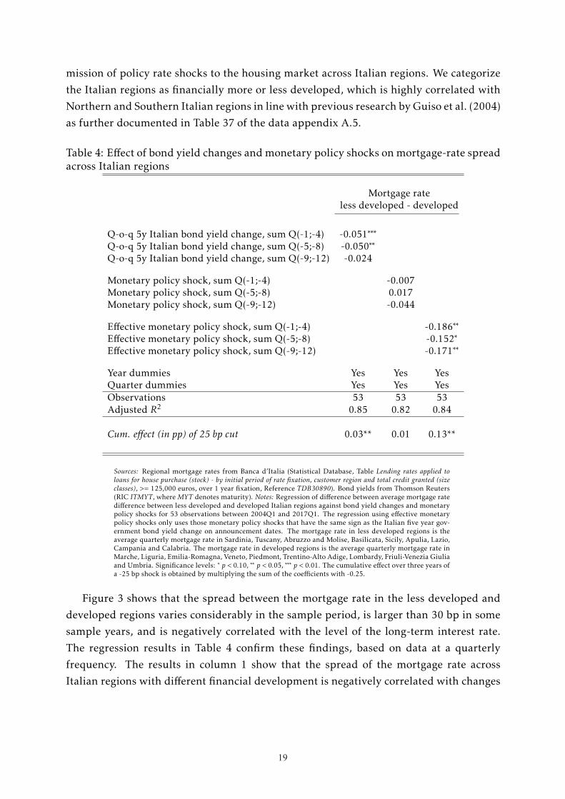
mission of policy rate shocks to the housing market across Italian regions. We categorize

the Italian regions as financially more or less developed, which is highly correlated with

Northern and Southern Italian regions in line with previous research by Guiso et al. (2004)

as further documented in Table 37 of the data appendix A.5.

Table 4: Effect of bond yield changes andmonetary policy shocks onmortgage-rate spreadacross Italian regions

Mortgage rateless developed - developed

Q-o-q 5y Italian bond yield change, sum Q(-1;-4) -0.051∗∗∗

Q-o-q 5y Italian bond yield change, sum Q(-5;-8) -0.050∗∗

Q-o-q 5y Italian bond yield change, sum Q(-9;-12) -0.024

Monetary policy shock, sum Q(-1;-4) -0.007Monetary policy shock, sum Q(-5;-8) 0.017Monetary policy shock, sum Q(-9;-12) -0.044

Effective monetary policy shock, sum Q(-1;-4) -0.186∗∗

Effective monetary policy shock, sum Q(-5;-8) -0.152∗

Effective monetary policy shock, sum Q(-9;-12) -0.171∗∗

Year dummies Yes Yes YesQuarter dummies Yes Yes YesObservations 53 53 53Adjusted R2 0.85 0.82 0.84

Cum. effect (in pp) of 25 bp cut 0.03** 0.01 0.13**

Sources: Regional mortgage rates from Banca d’Italia (Statistical Database, Table Lending rates applied toloans for house purchase (stock) - by initial period of rate fixation, customer region and total credit granted (sizeclasses), >= 125,000 euros, over 1 year fixation, Reference TDB30890). Bond yields from Thomson Reuters(RIC ITMYT, whereMYT denotes maturity). Notes: Regression of difference between average mortgage ratedifference between less developed and developed Italian regions against bond yield changes and monetarypolicy shocks for 53 observations between 2004Q1 and 2017Q1. The regression using effective monetarypolicy shocks only uses those monetary policy shocks that have the same sign as the Italian five year gov-ernment bond yield change on announcement dates. The mortgage rate in less developed regions is theaverage quarterly mortgage rate in Sardinia, Tuscany, Abruzzo and Molise, Basilicata, Sicily, Apulia, Lazio,Campania and Calabria. The mortgage rate in developed regions is the average quarterly mortgage rate inMarche, Liguria, Emilia-Romagna, Veneto, Piedmont, Trentino-Alto Adige, Lombardy, Friuli-Venezia Giuliaand Umbria. Significance levels: ∗ p < 0.10, ∗∗ p < 0.05, ∗∗∗ p < 0.01. The cumulative effect over three years ofa -25 bp shock is obtained by multiplying the sum of the coefficients with -0.25.

Figure 3 shows that the spread between the mortgage rate in the less developed and

developed regions varies considerably in the sample period, is larger than 30 bp in some

sample years, and is negatively correlated with the level of the long-term interest rate.

The regression results in Table 4 confirm these findings, based on data at a quarterly

frequency. The results in column 1 show that the spread of the mortgage rate across

Italian regions with different financial development is negatively correlated with changes

19

20

in long-term bond yields. The results in columns 2 and 3 show that the pass-through of

the policy rate shocks to the spread is only economically and statistically significant if we

consider policy rate shocks that are positively correlated with long-term yields (column

3). Once we implicitly exclude the euro-area debt crisis episode, in which the policy rate

shocks have been less effective in passing through to long-term yields, an unexpected 25

bp cut in the policy rate increases the spread by decreasing the mortgage rate by 13 bp

more in financially developed Italian regions.

5 Household data on housing markets

We use household-level data to analyze the transmission of monetary policy to the hous-

ing market. Given that we have shown in the previous section that policy rate shocks

pass through to mortgage interest rates and thus affect the user costs of households, the

household-level data allow us to investigate in detail the gross flows across housing tenure

states, the pass-through to rents and house prices, and the heterogeneity of this pass-

through across households with different ages, incomes, and net worth. Because we have

information on house prices only from the Italian and German household-level data, we

provide evidence for Switzerland on the pass-through to the price-rent ratio based on

aggregate data.16

We use microdata from the German Socioeconomic Panel (SOEP), the Italian Survey

of Household Income and Wealth (SHIW), and the Swiss Household Panel (SHP). For

Switzerland we complement the panel data with repeated cross-sectional data on rents

from the Swiss household budget survey (HABE). For Germany and Italy, information

on rents is available in the SOEP and SHIW. Further recent descriptions of the data are

provided by Goebel et al. (2019) for the SOEP, the Bank of Italy for the SHIW,17 Voorpostel

et al. (2017) for the SHP and BFS (2013) for the HABE.

Because households in the annual surveys for Germany and Switzerland are inter-

viewed across all quarters and the sample size is sufficiently large, we can use variation

across quarters during the period 2000Q1− 2016Q4. Because of the lagged independent

variables in the estimations, the sample for the estimation starts in 2003Q1 for both coun-

tries. The sample size is 138,682 for Germany, and 45,816 and 22,918, respectively, for

the samples obtained from the SHP and HABE datasets in Switzerland. The unit of obser-

vation is a household interviewed in a quarter of a given year. For Italy the sample size is

27,896 and the biannual survey frequency requires that we exploit variation across years

16For Germany we approximate the house value using information on mortgage payments, as explainedin data appendix A.5.

17See https://www.bancaditalia.it/statistiche/tematiche/indagini-famiglie-imprese/bilanci-famiglie/index.html .

20

20 21

during the same sample period. The Italian data have the advantage that we can exploit

in our analysis the regional heterogeneity in the pass-through to mortgage rates and the

housing market. We thus obtain further insights by using these regional differences to

identify the transmission of monetary policy to the housing market. Before we move on

to the analysis of the transmission, we provide descriptive evidence on some key charac-

teristics of the sample that we use for our analysis. We refer to the data appendix A.5 for

further details on the data sets and the sample construction.

Table 5: Homeownership and mortgage debt by age group

Ownership rate (%) Germany Italy Switzerland

Aged 25-44 36.8 62.0 38.5

Aged 45-64 58.2 79.6 61.8

Aged 65-84 60.0 84.6 58.7

Incidence of mortgagors (as % owners) Germany Italy Switzerland

Aged 25-44 78.5 36.5 81.9

Aged 45-64 53.9 20.1 80.9

Aged 65-84 16.4 4.9 67.4

Sources: SOEP (Germany), SHIW (Italy), SHP (Switzerland). Notes: Given the data availability, the inci-dence of mortgagors covers the 2002-2016 period for Germany, 2010-2016 for Italy, and 2014-2016 forSwitzerland. See Appendix A.5 for further details on the construction of the variables and the sample.

Table 5 displays in the top panel the familiar age profile of homeownership (of the

main residence) in Germany, Italy and Switzerland. As mentioned in Section 2, the home-

ownership rates in Germany and Switzerland are lower than in Italy.18 Table 5 shows

that this is true at all ages and that the ownership rate increases in all countries until re-

tirement. In Switzerland, the ownership rate falls slightly for retired households which

relates to the stronger response of the flow from owning to renting to policy rate shocks

that we report for Swiss households in the next Section 6.

The bottom panel of Table 5 shows that the incidence of mortgage debt is lower in

Italy than in Germany and Switzerland at all ages.19 During retirement the incidence

of mortgage debt is much larger in Switzerland than in Germany and Italy where most

18The averages of the owner occupation rate reported in Table 1 do not match exactly the averages acrossage groups based on the household-level data reported in Table 5 because they are based on a different datasource and period.

19This pattern is robust if we restrict the sample to new owners, i.e., renters who became owners betweenthe last and the current survey wave. The sizes of the subsamples are much smaller then, between 27 and128 for the age groups shown in Table 5.

21

22

households amortize their mortgage until retirement and then own their home outright.

This different amortization behavior in Switzerland is related to different tax incentives

for amortization as further analyzed in Koeniger et al. (2021).

01

23

45

6

2001

2002

2003

2004

2005

2006

2007

2008

2009

2010

2011

2012

2013

2014

2015

2016

2017


Households who changed tenure (% of households)

01

23

45

6

2001

2002

2003

2004

2005

2006

2007

2008

2009

2010

2011

2012

2013

2014

2015

2016

2017


Renters who became owners (% of renters)

01

23

45

6

2001

2002

2003

2004

2005

2006

2007

2008

2009

2010

2011

2012

2013

2014

2015

2016

2017


Owners who became renters (% of owners)

Sources: SOEP (Germany), SHIW (Italy), SHP (Switzerland). Notes: Annual average flows. For Italy, biannualflows are annualized. Appendix A.6 contains detailed information about how the flows are annualized.

Figure 4: Housing tenure flows over time

The age profiles of the homeownership rates in the top panel of Table 5 suggest that

households change housing tenure status. Figure 4 provides explicit information on the

transition rates. The left plot displays the percentage of households that have changed

housing tenure between the current and previous survey wave. Figure 4 also provides

information on the separate flows, from renting to owning and vice versa. The middle

plot shows the renters who have become owners (as a percentage of the sample of renters),

and the right plot shows the owners who have become renters (as a percentage of owners).

The plots in Figure 4 show that twice as many households change housing tenure per

year in Germany and Switzerland than in Italy. On average around 4% of renters per

year become homeowners in all three considered countries.20 The percentage of owners

that become renters per year is lower on average, about 2% in Germany and Switzerland.

In Italy, homeownership seems more like an absorbing state, given that less than 1% of

owners become renters. We exploit the variation in the flows between different types ofhousing tenure, across quarters and years, to identify the effect of the monetary policy

shocks on changes in housing tenure.

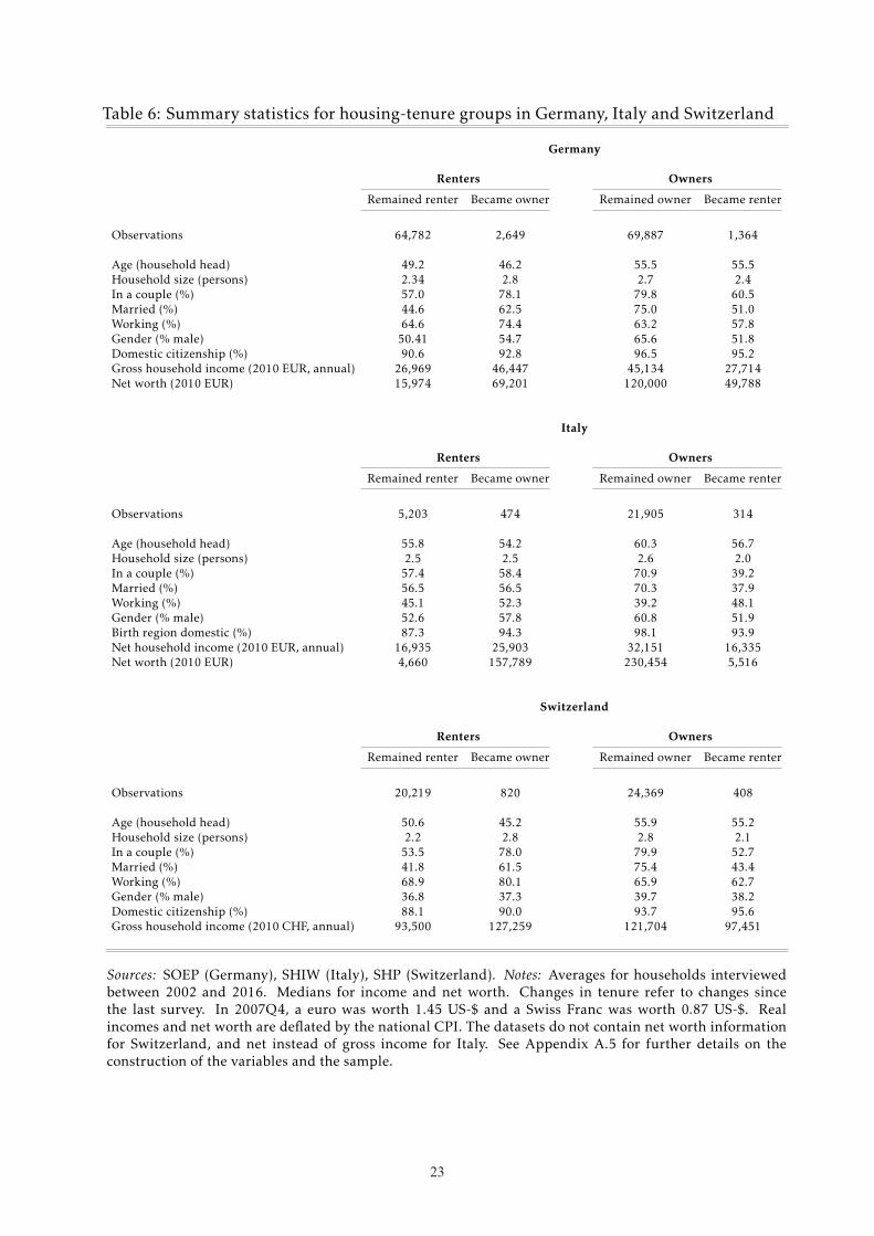
Table 6 provides summary statistics for the different housing tenure groups in Ger-

many, Italy and Switzerland. As noted by Andrews and Sanchez (2011a,b), the marginal

20The transition rates are annualized for Italy given the biannual frequency of the survey, as explainedfurther in Appendix A.6. When comparing the transition rates from rental to owning across countries, onehas to consider that fewer households rent in Italy than in Germany and Switzerland. The transition ratesin the considered countries are approximately half of those in the U.S. reported by Ma and Zubairy (2021),Figure 4, once the rates they report are annualized to make them comparable.

22

22 23

Table 6: Summary statistics for housing-tenure groups in Germany, Italy and Switzerland

Germany

Renters XXX Owners

Remained renter Became owner Remained owner Became renter

Observations 64,782 2,649 69,887 1,364

Age (household head) 49.2 46.2 55.5 55.5Household size (persons) 2.34 2.8 2.7 2.4In a couple (%) 57.0 78.1 79.8 60.5Married (%) 44.6 62.5 75.0 51.0Working (%) 64.6 74.4 63.2 57.8Gender (% male) 50.41 54.7 65.6 51.8Domestic citizenship (%) 90.6 92.8 96.5 95.2Gross household income (2010 EUR, annual) 26,969 46,447 45,134 27,714Net worth (2010 EUR) 15,974 69,201 120,000 49,788

Italy

Renters XXX Owners


Observations 5,203 474 21,905 314

Age (household head) 55.8 54.2 60.3 56.7Household size (persons) 2.5 2.5 2.6 2.0In a couple (%) 57.4 58.4 70.9 39.2Married (%) 56.5 56.5 70.3 37.9Working (%) 45.1 52.3 39.2 48.1Gender (% male) 52.6 57.8 60.8 51.9Birth region domestic (%) 87.3 94.3 98.1 93.9Net household income (2010 EUR, annual) 16,935 25,903 32,151 16,335Net worth (2010 EUR) 4,660 157,789 230,454 5,516

Switzerland

Renters XXX Owners


Observations 20,219 820 24,369 408

Age (household head) 50.6 45.2 55.9 55.2Household size (persons) 2.2 2.8 2.8 2.1In a couple (%) 53.5 78.0 79.9 52.7Married (%) 41.8 61.5 75.4 43.4Working (%) 68.9 80.1 65.9 62.7Gender (% male) 36.8 37.3 39.7 38.2Domestic citizenship (%) 88.1 90.0 93.7 95.6Gross household income (2010 CHF, annual) 93,500 127,259 121,704 97,451

Sources: SOEP (Germany), SHIW (Italy), SHP (Switzerland). Notes: Averages for households interviewedbetween 2002 and 2016. Medians for income and net worth. Changes in tenure refer to changes sincethe last survey. In 2007Q4, a euro was worth 1.45 US-$ and a Swiss Franc was worth 0.87 US-$. Realincomes and net worth are deflated by the national CPI. The datasets do not contain net worth informationfor Switzerland, and net instead of gross income for Italy. See Appendix A.5 for further details on theconstruction of the variables and the sample.

23

24

worth. In our analysis, we thus allow for a heterogeneous pass-through in some specifica-

tions.

6 The response of housing tenure

In this section we estimate the effect of monetary policy shocks on housing tenure in

Germany, Italy and Switzerland. Because the shocks may induce home purchases or sales,

we estimate the effect on both the transition from being a renter to becoming a homeowner

and vice versa. Homeownership refers to owner occupation of the primary residence in

the data sets and does not include ownership of second homes.

We find that a monetary policy shock triggers adjustments in the housing market:

some renters become homeowners and, simultaneously, some homeowners become renters.

The net effect on owner occupation is positive for an accommodative shock, suggesting

that the positive demand effect resulting from such a shock does not only imply higher

house prices. We now present our findings in further detail.

We exploit variation at a quarterly frequency for Germany and Switzerland because

we have information on the interview date of households. For Italy we use the annual

variation in the shocks and biannual transitions given the lower survey frequency. We

discuss the resulting differences in the subsequent regression specifications. The reported

cumulated effects for Italy based on biannual transitions are adjusted to be comparable

with those for Germany and Switzerland based on annual transitions, as explained further

in Appendix A.6.

Given that households in the German and Swiss panel data are interviewed at an an-

nual frequency, we pool all of the observations on renters to estimate the probability of

becoming a homeowner in each quarter and year, and we pool all of the observations on

homeowners to estimate the probability of becoming a renter. Households who change

housing tenure more than once are captured at each change. Age controls in the regres-

sion account for differences in the transition probabilities across age groups.

We use the panel dimension of the surveys to construct a dummy variable for changes

in housing tenure during the last year. For household i from region r interviewed in

quarter q and year t we define

Changeirqt =

1 if the housing tenure changed,

0 otherwise.

We estimate a linear probability model and provide robustness results for non-linear

25

home buyers and sellers in Germany, Italy and Switzerland may be different because of

differences in tax incentives and regulation associated with differences in house prices (see

also the references therein). To shed light on the characteristics of the households that

change housing tenure status, we distinguish renters that have remained renters (since

the last survey) from renters that have become homeowners, and we distinguish home-

owners that have remained owners from those that have become renters. Table 6 shows

that, as one would expect, renters that have become homeowners tend to be younger than

those who have remained renters. They have higher incomes, are more likely to work,

and have higher net worth (in Germany and Italy, for which data on net worth are avail-

able). In Germany and Switzerland, the size of households that have become homeowners

is larger and these households are more likely to be composed of married individuals or

those living as a couple. The transition from homeownership to rental occurs at later ages,

on average previous to retirement. Table 6 shows that owners that become renters have

relatively less income and lower net worth (in Germany and Italy, for which data on net

worth are available). They are less likely to be married or to live as a couple, implying

smaller household sizes.

Across countries, renters that become owners are older in Italy than in Germany and

Switzerland whichmay be related to household formation in Italy occuring later in the life

cycle. Moreover, the differences in net-worth positions associated with changes of hous-

ing tenure are larger in Italy than in Germany. To understand this further, we inspect

the net-worth position of households in Italy in the survey wave previous to the change

of their housing tenure. We find that the median net worth of renters who have become

owners is 7,505 euro, which is only somewhat larger before the transition than the net

worth of households that remained renters. Moreover, the median net worth of 160,539

euro held by owners, before they become renters in the subsequent survey wave, has the

same order of magnitude as the net worth of households that have remained owners. The

large amount of additional wealth that renters report when they become owners, and the

much smaller amount of wealth which owners report after they become renters, suggest

that transfers across households, possibly across generations, are associated with hous-

ing tenure transitions in Italy. This evidence is in line with the much lower incidence of

mortgages in Italy that we have reported in Table 5. Beyond these differences, the charac-teristics of the respective subpopulations appear quite similar across the three considered

countries. Table 38 in Appendix A.5 shows that this also applies to Italian regions with

different financial development.

The patterns in the characteristics of the marginal populations that change housing

tenure status suggest that the pass-through of policy shocks to housing tenure transitions

may be heterogeneous, for example across groups with different ages, incomes, or net

24

24 25

worth. In our analysis, we thus allow for a heterogeneous pass-through in some specifica-

tions.

6 The response of housing tenure

In this section we estimate the effect of monetary policy shocks on housing tenure in

Germany, Italy and Switzerland. Because the shocks may induce home purchases or sales,

we estimate the effect on both the transition from being a renter to becoming a homeowner

and vice versa. Homeownership refers to owner occupation of the primary residence in

the data sets and does not include ownership of second homes.

We find that a monetary policy shock triggers adjustments in the housing market:

some renters become homeowners and, simultaneously, some homeowners become renters.

The net effect on owner occupation is positive for an accommodative shock, suggesting

that the positive demand effect resulting from such a shock does not only imply higher

house prices. We now present our findings in further detail.

We exploit variation at a quarterly frequency for Germany and Switzerland because

we have information on the interview date of households. For Italy we use the annual

variation in the shocks and biannual transitions given the lower survey frequency. We

discuss the resulting differences in the subsequent regression specifications. The reported

cumulated effects for Italy based on biannual transitions are adjusted to be comparable

with those for Germany and Switzerland based on annual transitions, as explained further

in Appendix A.6.

Given that households in the German and Swiss panel data are interviewed at an an-

nual frequency, we pool all of the observations on renters to estimate the probability of

becoming a homeowner in each quarter and year, and we pool all of the observations on

homeowners to estimate the probability of becoming a renter. Households who change

housing tenure more than once are captured at each change. Age controls in the regres-

sion account for differences in the transition probabilities across age groups.

We use the panel dimension of the surveys to construct a dummy variable for changes

in housing tenure during the last year. For household i from region r interviewed in

quarter q and year t we define

Changeirqt =

1 if the housing tenure changed,

0 otherwise.

We estimate a linear probability model and provide robustness results for non-linear

25

26

probit and logit specifications in Appendix A.2.7. The regression specification is

Changeirqt = α + β′zqt +γ ′xirqt +Dr +Dq +Dt + εirqt ,

where Changeirqt is the binary variable previously described, and the vector zqt denotesthe monetary policy shocks in the last three years, cumulated over quarters separately for

each of the years.21 The vector xirqt contains a set of control variables, which vary at the

household level.22 In all of the regression specifications we control for common effectsby quarter Dq and year Dt , and thus control for common trends and seasonal effects.In some specifications we also control for common effects by region Dr , or we allow for

heterogeneous effects across population groups with different ages, incomes, and wealth.

The identification of these effects exploits the cross-sectional variation in the household

data.

The estimation of our specification is straightforward given that the monetary policy

shocks have been constructed to be exogenous. The year-quarter variation identifies the

effect of the monetary policy shocks in our regressions for Germany and Switzerland.

In the specifications for Italy, identification is based on the annual deviations from the

trend, and on the region-year variation for the specifications presented in Section 8. To

preserve degrees of freedom, we estimate a parsimonious specification. We cumulate

shocks per year and allow for lagged effects of shocks up to three years. In Appendix A.2.5

we show that including additional lags of the shocks amplifies the benchmark results for

the transitions from renting to owning that we subsequently present, at the cost of less

degrees of freedom, such that the main specification provides conservative estimates.23

Table 7 summarizes the results for the effect of monetary policy shocks on housing

tenure in Germany, Italy and Switzerland. In the benchmark specification reported in

21For Italy the regression specification modifies to

Changeirt = α + β′zt +γ ′xirt + δt +Dr + εirt ,

given that the survey frequency requires that we cumulate shocks zt by year. Thus, the coefficients β areidentified by annual variation where we control for a common linear time trend. In the specifications, inwhich we identify the effect of policy rate shocks by exploiting regional differences, we add interactionsof the shocks zt with a dummy for financially developed regions and control for aggregate time effectsmore flexibly by adding time dummies. The coefficients of interest are then identified by the region-yearvariation.

22We do not use aggregate variables as controls because doing so would contaminate our regression spec-ification. For example, unemployment and real GDP growth affect monetary policy decisions and, simulta-neously, are influenced by them so that these variables are endogenous. If our constructed monetary policyshocks are exogenous and thus are true surprises, which we have attempted to achieve with our constructionof the series, omitted variables are uncorrelated with these shocks and do not bias the coefficient estimates.

23For Italy we can include less additional lags because we have less degrees of freedom. Given thatthe additional lags reduce the length of the sample period that we can use for our estimation, we displayestimates in Table 22 in Appendix A.2.5 for the benchmark specification on the smaller sample for ease ofcomparison, together with the estimates for the specifications with the additional lags of the shocks.

26

26 27

Table 7, the different data frequencies across countries, as previously explained, imply

that we control for year and quarter dummies for Germany and Switzerland and a linear

time trend for Italy. We cluster standard errors by quarter of interview for Germany and

Switzerland and by year for Italy because the monetary policy shocks do not vary at the

household level. In Appendix A.2.6 we show that our results are robust if we add addi-

tional controls for household characteristics on which we presented descriptive evidence

in Table 6. Thus, the observable heterogeneity in the sample composition in each of the

considered countries does not explain the different transmission of monetary policy to the

housing market across countries which we find.

Table 7: Effect of monetary policy shocks on housing tenure transitions

Renter to owner Owner to renter

Germany Italy Switzerland Germany Italy Switzerland

Monetary policy shock, sum Q(-1,-4) -0.019 -0.024** -0.032*** 0.002 -0.003* -0.017***Monetary policy shock, sum Q(-5,-8) -0.030* 0.065** -0.017*** 0.001 0.008 -0.004Monetary policy shock, sum Q(-9,-12) -0.025* 0.069*** -0.004 0.002 0.007** 0.003

Age controls Yes Yes Yes Yes Yes YesQuarter dummies Yes No Yes Yes No YesYear dummies Yes No Yes Yes No YesLinear trend No Yes No No Yes NoObservations 67,431 5,677 21,039 71,251 22,219 24,777Adjusted R2 0.00 0.01 0.01 0.00 0.00 0.01

Cum. annualized effect (in pp) of 25 bp cut 1.82* -1.37*** 1.32*** -0.13 -0.15* 0.46***

Notes: Significance levels: ∗ p < 0.10, ∗∗ p < 0.05, ∗∗∗ p < 0.01. The dependent variable is 1 if a householdchanged tenure status and 0 if it does not. Standard errors are clustered by quarter of the interviewfor Germany and Switzerland and by year for Italy, because the monetary policy shock does not vary atthe household level. Age controls include age and age squared and refer to the household’s referenceperson. The cumulative effect over three years of a -25 bp shock is obtained by multiplying the sum of thecoefficients with -0.25. The reported cumulative effects for Italy based on biannual transitions are adjustedto be comparable with those for Germany and Switzerland based on annual transitions.

Table 7 shows that the monetary policy shocks affect housing tenure choices signifi-

cantly in all countries.24 The quantitative patterns are quite different though. The im-

mediate effect on housing tenure transitions within a year of the shocks is strongest in

Switzerland for the transitions from rental to owning and vice versa. This is in line with

24The low adjusted R2 in Table 7 illustrates that much of the variation at the household level remainsunexplained. This is not surprising because the only variable, that enters the regressions and varies at thehousehold level, is age. Because our goal is to estimate the causal effect of policy rate shocks and not topredict the transitions, we have refrained from adding more variables in our benchmark specification thatmay improve the predictive power at the cost of introducing endogeneity issues. As previously discussed,omitted variable bias is not a concern given the exogeneity of the shocks.

27

28

our finding in subsection 4.2 that the pass-through of policy rate shocks to mortgage rates

is strongest in Switzerland. The implied change of the user cost seems particularly rel-

evant for younger households for their transition from rental to owning as subsequently

discussed. The transitions from owning to renting seem driven more by the effect of thepolicy rate shock on price-rent ratios, given that this transition is more relevant for older

households who are relatively less leveraged. As is is shown in the next Section 7, rents

in Switzerland respond immediately and most strongly to the policy rate shocks, possibly

because of the indexation of rents to mortgage rates discussed in Section 2.

The coefficients of the shocks with further lags in Table 7 reveal that the policy rate

shocks affect the timing of housing tenure transitions in Italy but the effects are not per-

sistent as in Switzerland and Germany. This is illustrated by the opposite sign of the

coefficients of the shocks at short and longer lags in Italy compared with the same sign of

these coefficients in Germany and Switzerland. In Germany, the policy rate shocks only

affect the transition from owning to renting, and more so at longer lags. As we document

in Section 7, this pattern is similar for the effect of the interest rate shocks on rents and

house prices which is stronger at longer lags in Germany than in Italy and Switzerland.

In the bottom row of Table 7, we report the total effect of an unexpected 25 bp interest

rate cut.25 We find that the transition from renting to owning increases by 1 − 2 pp in

Germany and Switzerland. In Italy, the initial increase is more than offset over time,

implying a decrease in the transition by 1.4 pp. The negative total effect in Italy becomes

smaller (in absolute terms) and is insignificant if we use shocks to long-term yields on

announcements dates instead of policy rate shocks, as shown in Table 19 in Appendix

A.2.2. The pass-through of policy rate shocks to rates of long-term bonds and mortgages

has been less effective in Italy during the sovereign debt crisis in our sample period, as

discussed in Section 4.2.

Thus, the robust finding for Italy is that the transmission of interest rate changes to

housing tenure transitions is weaker than in Germany and Switzerland, a result associated

with the strong pass-through to house prices in the quarters after an interest rate cut, as

shown in Table 10 in Section 7. Moreover, the descriptive evidence in Table 6 in Section

5 suggests that other determinants, such as (intergenerational) transfers across house-

holds, are associated with housing tenure transitions in Italy, which is in line with the

much smaller incidence of mortgages. Thus, the smaller pass-through of monetary policy

shocks to housing tenure transitions in Italy may not be surprising after all. Interestingly,

the relative effect of the monetary policy shocks on housing tenure transitions across Ital-

ian regions with different financial development is more similar to the aggregate effects on

25Note that we use a change by 25 bp for the quantitative illustration. We do this because the response toshocks of this size is usually reported. The typical unexpected shock to the policy rate is much smaller inour sample period, as shown in Figure 1 in Section 3.

28

28 29

housing tenure transitions estimated for Germany and Switzerland, as discussed further

in Section 8.

The bottom row of Table 7 further shows that an unexpected reduction in the inter-

est rate increases the transition from owning to renting by 0.5 pp in Switzerland. For

Germany and Italy, we find no strong effect on the transition from owning to renting. It

decreases slightly and not significantly for Germany. For Italy, the decrease by 0.15 pp is

only significant at the 10%-level.

When interpreting the size of the effects, it is important to recall that typical policy rate

shocks are much smaller than 25 bp. As mentioned in Section 3, the standard deviation

of the monetary policy shocks is 7 bp for the ECB and 10 bp for the SNB. Thus, the effectson the transitions reported in Table 7 must be scaled down by approximately one third

if we consider a policy rate shock of one standard deviation. The scaled effects remain

quantitatively relevant given that around 4 percent of renters become homeowners per

year and 1− 2 percent of owners become renters, as we have shown in Figure 4 in Section

5.

Table 8 provides evidence on the heterogeneity of the transmission across groups with

different ages, incomes and net worth. Information on the latter is only available in the

German and Italian data. We choose to report the heterogeneity for age, income and net

worth because the descriptive evidence presented in Table 6, Section 5, suggested that the

subpopulations that change housing tenure status differ in these dimensions from the rest

of the population. Furthermore, age, income and net worth are state variables in typical

structural models of household financial behavior so that they are of particular interest.

Table 8 displays the cumulated effects of an unexpected 25 bp cut by subgroup. The effectreported in each cell of the table is obtained by estimating the benchmark regression

specification for each subgroup. The results for the entire sample are repeated in the first

row for ease of comparison.

Table 8 confirms the suggestive descriptive evidence in Table 6. The results in columns

1 to 3 show that the policy rate shocks in Germany and Switzerland trigger more transi-

tions from rental to owning for relatively younger households, for households with in-

come higher than the median, and for households with a higher net worth (for Germany).

The patterns for Italian households are less clear cut which is related to the finding that

the response of the transition to homeownership has a more complicated timing and is

different to Germany and Switzerland, as shown in Table 7.

Regarding the transition from owning to renting, columns 4 to 6 in Table 8 show that

the sizable increase after a policy rate cut in Switzerland is caused by households with

a head between ages 45 and 64 before retirement, particularly if they have a lower than

median income. For Italy, a policy rate cut reduces the transition from owning to renting

29

our finding in subsection 4.2 that the pass-through of policy rate shocks to mortgage rates

is strongest in Switzerland. The implied change of the user cost seems particularly rel-

evant for younger households for their transition from rental to owning as subsequently

discussed. The transitions from owning to renting seem driven more by the effect of thepolicy rate shock on price-rent ratios, given that this transition is more relevant for older

households who are relatively less leveraged. As is is shown in the next Section 7, rents

in Switzerland respond immediately and most strongly to the policy rate shocks, possibly

because of the indexation of rents to mortgage rates discussed in Section 2.

The coefficients of the shocks with further lags in Table 7 reveal that the policy rate

shocks affect the timing of housing tenure transitions in Italy but the effects are not per-

sistent as in Switzerland and Germany. This is illustrated by the opposite sign of the

coefficients of the shocks at short and longer lags in Italy compared with the same sign of

these coefficients in Germany and Switzerland. In Germany, the policy rate shocks only

affect the transition from owning to renting, and more so at longer lags. As we document

in Section 7, this pattern is similar for the effect of the interest rate shocks on rents and

house prices which is stronger at longer lags in Germany than in Italy and Switzerland.

In the bottom row of Table 7, we report the total effect of an unexpected 25 bp interest

rate cut.25 We find that the transition from renting to owning increases by 1 − 2 pp in

Germany and Switzerland. In Italy, the initial increase is more than offset over time,

implying a decrease in the transition by 1.4 pp. The negative total effect in Italy becomes

smaller (in absolute terms) and is insignificant if we use shocks to long-term yields on

announcements dates instead of policy rate shocks, as shown in Table 19 in Appendix

A.2.2. The pass-through of policy rate shocks to rates of long-term bonds and mortgages

has been less effective in Italy during the sovereign debt crisis in our sample period, as

discussed in Section 4.2.

Thus, the robust finding for Italy is that the transmission of interest rate changes to

housing tenure transitions is weaker than in Germany and Switzerland, a result associated

with the strong pass-through to house prices in the quarters after an interest rate cut, as

shown in Table 10 in Section 7. Moreover, the descriptive evidence in Table 6 in Section

5 suggests that other determinants, such as (intergenerational) transfers across house-

holds, are associated with housing tenure transitions in Italy, which is in line with the

much smaller incidence of mortgages. Thus, the smaller pass-through of monetary policy

shocks to housing tenure transitions in Italy may not be surprising after all. Interestingly,

the relative effect of the monetary policy shocks on housing tenure transitions across Ital-

ian regions with different financial development is more similar to the aggregate effects on

25Note that we use a change by 25 bp for the quantitative illustration. We do this because the response toshocks of this size is usually reported. The typical unexpected shock to the policy rate is much smaller inour sample period, as shown in Figure 1 in Section 3.

28

30

Table 8: Cumulative effect of 25 bp cut on housing tenure transitions for groups withdifferent ages, income and net worth



Whole sample 1.82* -1.37*** 1.32*** -0.13 -0.15* 0.46***

By age groupAge 25-44 2.94** -1.59 1.14** -0.17 -1.15*** -1.23*Age 45-64 1.06 -0.77** 1.69*** -0.26 -0.06 1.41***Age 65-84 -1.94 -1.92** 0.95*** -0.19 0.03 -0.26

By income, working age group (25-64),Working age group (25-64) 2.35** -1.11*** 1.28*** -0.16 -0.29** 0.75***Incomes < median 0.52 -1.34*** 0.58*** 1.47* -0.32* -0.10Incomes > median 3.77** -0.72 1.82*** -0.82** -0.20** 1.07***

Incomes < median (within age group):Age 25-44 0.25 -1.78* 0.16 6.38*** -2.15** -4.14*Age 45-64 0.31 -1.03* 0.89*** -0.78 0.11 1.77***Age 65-84 -1.19 -1.37 -0.91** -0.64 0.06 2.35***

Incomes > median (within age group):Age 25-44 4.69** -0.94 1.88** -2.48** -0.48* -0.04Age 45-64 1.93 0.24 1.59** -0.01 -0.12*** 1.41***Age 65-84 -3.10 -2.55 4.35*** 0.27 0.06 -2.02***

By net worth, working age group (25-64),Working age group (25-64) 2.35** -1.11*** - -0.16 -0.29** -Net worth < median 1.32 -0.21 - -0.44 -1.07*** -Net worth > median 2.59** -10.82*** - -0.04 0.02 -

Net worth < median (within age group):Age 25-44 2.92** -0.79*** - -0.50 -7.64*** -Age 45-64 0.31 0.17 - -0.28 -0.44 -Age 65-84 -2.44 -0.34 - -1.15 0.07 -

Net worth > median (within age group):Age 25-44 2.70* -7.49 - 0.13 -0.23** -Age 45-64 1.87 -14.40*** - -0.24 0.11** -Age 65-84 -1.24 -4.39 - 0.02 0.05** -

Notes: Significance levels: ∗ p < 0.10, ∗∗ p < 0.05, ∗∗∗ p < 0.01. The dependent variable is 1 if a householdchanged tenure status and 0 if it does not. Standard errors are clustered by quarter of the interview forGermany and Switzerland and by year for Italy, because the monetary policy shock does not vary at thehousehold level. Age controls include age and age squared and refer to the household’s reference person.The reported cumulative annualized effect is in pp. The estimates for Italy based on biannual transitionsare adjusted to be comparable with those for Germany and Switzerland based on annual transitions.Subgroups consist of at least 105 observations. The typical subgroup has more than 1,000 observations.

30

30 31

for young households with lower income and net worth. Thus, the different response of

the transition from owning to renting in Switzerland and Italy seems to be related to the

higher homeownership rates of young households in Italy relative to Switzerland.

Given that some research has emphasized the importance of cultural factors for finan-

cial decisions of households, we exploit the diversity of languages within Switzerland to

assess whether the patterns found across countries are also present within Swiss cantons

across language groups. We assign themembership in a language group according to what

the household head considers as the first language.26 The reference language is Swiss Ger-

man, and the dummiesGerman, French and Italian refer to households in Switzerland with

a German, French and Italian mother tongue, respectively. We add household controls to

the regression because the descriptive statistics displayed in Tables 35 and 36 in Appendix

A.5 show that language groups differ in observables such as age and income which may

affect the response to monetary-policy shocks. We add canton dummies as further con-

trols to capture differences across these cantons, for example in terms of regulations, and

we also add canton-year dummies to capture changes in these regulations over time.

Table 9 shows that our benchmark results are robust to adding these additional con-

trols, and that housing tenure transitions respond similarly to monetary policy shocks

across language groups within Swiss cantons. For ease of comparison, columns 1 and 3

of Table 9 display the estimates for the effect of the monetary policy shocks on housing

tenure transitions if we just add the household controls to the benchmark specification.

In columns 2 and 4 of Table 9 we add interactions of the monetary policy shocks with

dummies for the respective language group, and control for canton and canton-year fixed

effects. The joint F-test for the significance of the language-shock interactions has a p-

value higher than 18% for the regression on the transitions from renting to owning in

column 2. For the regression on the transitions from owning to renting reported in col-

umn 4, households with French and Italian mother tongue do not respond differently to

households with a Swiss-German mother tongue. The F-test for each group has a p-value

higher than 42%. The only heterogeneity in the housing tenure responses across language

groups which we detect is that households with a German mother tongue are more likely

to transit from owning to renting after a interest rate cut than households with a Swiss-

Germanmother tongue. The p-value of the F-test is 1%when we test the joint significance

of the coefficients for the German-language interactions with the monetary policy shocks.

Overall, we find little evidence for different responses across language groups within

26The first language is reported for 19,474 out of 45,816 households. To ensure a sufficient sample sizeacross quarters in the considered period, we assign the language according to the location of the residencefor the remaining households. In Appendix A.5, Tables 35 and 36 show that the subsample of householdswho report a first language has similar observable characteristics across language groups as does the samplethat we use.

31

32

Table 9: Effect of monetary policy shocks on housing tenure, across language groups inSwitzerland


(1) (2) (3) (4)

Monetary policy shock, sum Q(-1,-4) -0.029*** -0.036*** -0.018*** -0.020***Monetary policy shock, sum Q(-5,-8) -0.013*** -0.007 -0.008*** -0.008*Monetary policy shock, sum Q(-9,-12) -0.002 0.005 0.000 0.007Monetary policy shock, sum Q(-1,-4) × German -0.023 -0.004Monetary policy shock, sum Q(-5,-8) × German 0.035 -0.048**Monetary policy shock, sum Q(-9,-12) × German 0.028 -0.049Monetary policy shock, sum Q(-1,-4) × Italian -0.022 -0.015Monetary policy shock, sum Q(-5,-8) × Italian -0.035 0.002Monetary policy shock, sum Q(-9,-12) × Italian -0.050 -0.003Monetary policy shock, sum Q(-1,-4) × French 0.024 0.013Monetary policy shock, sum Q(-5,-8) × French -0.019 0.003Monetary policy shock, sum Q(-9,-12) × French -0.030 -0.022

Household controls† Yes Yes Yes YesQuarter dummies Yes Yes Yes YesYear dummies Yes Yes Yes YesCanton dummies No Yes No YesCanton-year dummies No Yes No YesObservations 21,039 21,039 24,777 24,777Adjusted R2 0.02 0.04 0.02 0.02

Cum. effect (in pp) of 25 bp cut 1.10*** 0.95** 0.66*** 0.53**

Notes: Significance levels: ∗ p < 0.10, ∗∗ p < 0.05, ∗∗∗ p < 0.01. †: Household controls also use information onthe household’s reference person and include: age, age squared, household size, civil status, partnership,working status, gender, nationality, real household income. The dependent variable is 1 if a householdchanged tenure status and 0 if it does not. Language interactions use the first language of the household’shead; the reference language is Swiss-German. Standard errors are clustered by quarter of the interview,because the monetary policy shock does not vary at the household level. The cumulative effect over threeyears of a -25 bp shock is obtained by multiplying the sum of the coefficients with -0.25.

32

32 33

Switzerland. This finding suggests that cultural differences may not be of first-order im-

portance for understanding the cross-country differences in the pass-through of monetary

policy shocks to housing tenure transitions, which we reported in Table 7. Instead, the

differences in housing markets across these countries discussed in Section 2, and the dif-

ferent pass-through of themonetary policy shocks to themortgage interest rates discussed

in Section 4.2 seem to play an important role.

6.1 Robustness

Appendix A.2 contains all of the robustness checks for the main regression specification

reported in Table 7. We discuss the results to which we have not yet referred. In Appendix

A.2.1, we provide robustness checks for alternative time windows around the policy an-

nouncements. Specifically, we construct policy rate shocks using six-hour time windows

as in Corsetti et al. (2020) for constructing policy rate shocks, and 30-minute time win-

dows as in Nakamura and Steinsson (2018). Table 16 in Appendix A.2.1 shows that the

correlation between these shocks series and our benchmark series is high except for the

series based on 30-minute time windows in the euro area. The communication of mone-

tary policy by the ECB requires longer time windows than 30 minutes to capture all of the

new information released. Thus, we report robustness checks for the euro-area countries

Germany and Italy using the series for monetary policy shocks based on a six-hour time

window, as in Corsetti et al. (2020). For Switzerland, we report the robustness results for

both the shock series based on the six-hour and the 30-minute time window.

Tables 17 and 18 in Appendix A.2.1 show that the estimated effects on housing tenure

transitions are robust to using the alternative time windows. The coefficient estimates

tend to become larger if we use shocks based on shorter time windows. This result should

be expected given the timing of the announcements and the subsequent press conferences

which we have described in Section 3. The shocks are smaller if measured over shorter

time windows because the full effect of the announcement takes longer to pass through to

the futures market, particularly so for the very short 30-minute time window. We view the

benchmark time window of one day, between the end of the announcement day and the

day before, as a reasonable compromise between capturing the full effect of the monetary

policy announcement on the futures prices and avoiding that other changes in that time

window confound the results.

Table 19 in Appendix A.2.2 shows that the responses of housing tenure transitions

from renting to owning are very similar in Germany and Switzerland if we use unexpected

changes in the five-year government bond yields on the announcement days. For Italy, the

responses become less different to Germany and Switzerland compared with our bench-

mark results. The remaining difference in the responses of housing tenure transitions

33

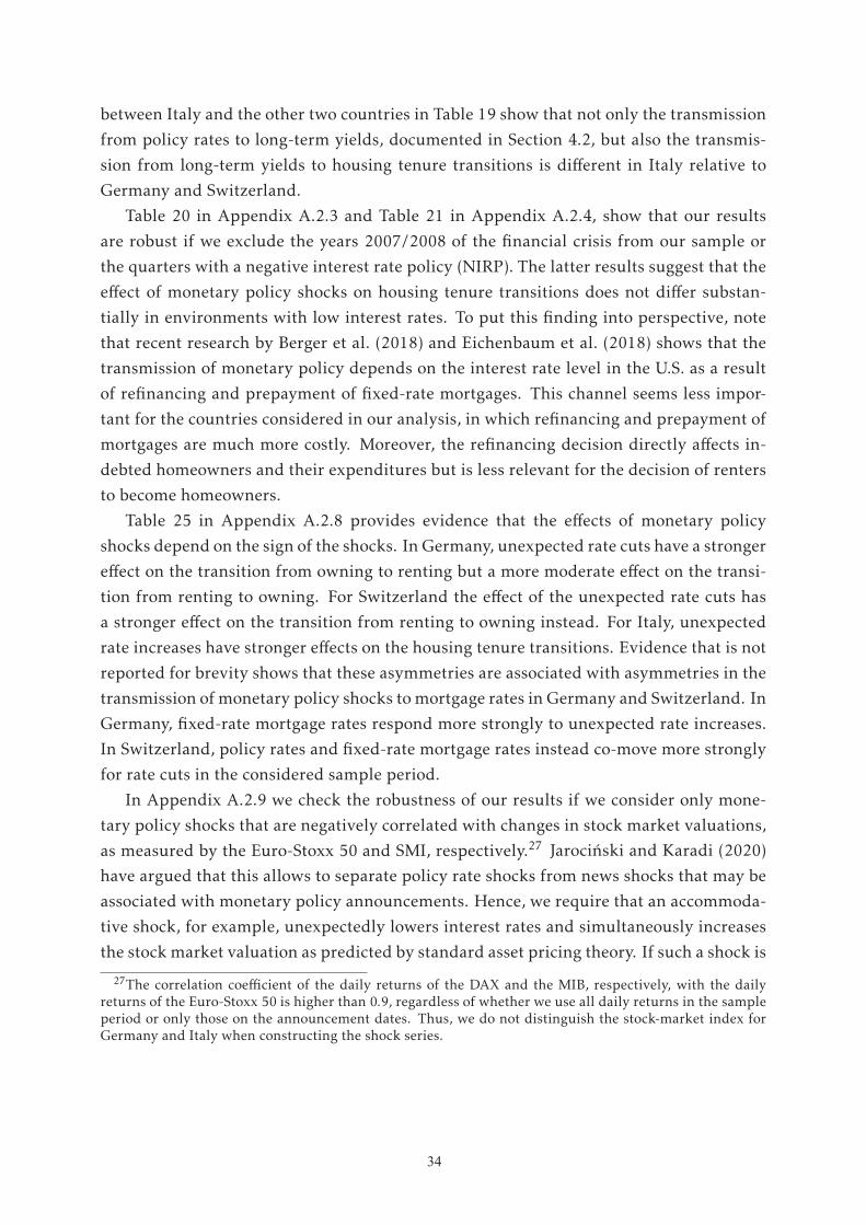
34

between Italy and the other two countries in Table 19 show that not only the transmission

from policy rates to long-term yields, documented in Section 4.2, but also the transmis-

sion from long-term yields to housing tenure transitions is different in Italy relative to

Germany and Switzerland.

Table 20 in Appendix A.2.3 and Table 21 in Appendix A.2.4, show that our results

are robust if we exclude the years 2007/2008 of the financial crisis from our sample or

the quarters with a negative interest rate policy (NIRP). The latter results suggest that the

effect of monetary policy shocks on housing tenure transitions does not differ substan-

tially in environments with low interest rates. To put this finding into perspective, note

that recent research by Berger et al. (2018) and Eichenbaum et al. (2018) shows that the

transmission of monetary policy depends on the interest rate level in the U.S. as a result

of refinancing and prepayment of fixed-rate mortgages. This channel seems less impor-

tant for the countries considered in our analysis, in which refinancing and prepayment of

mortgages are much more costly. Moreover, the refinancing decision directly affects in-debted homeowners and their expenditures but is less relevant for the decision of renters

to become homeowners.

Table 25 in Appendix A.2.8 provides evidence that the effects of monetary policy

shocks depend on the sign of the shocks. In Germany, unexpected rate cuts have a stronger

effect on the transition from owning to renting but a more moderate effect on the transi-

tion from renting to owning. For Switzerland the effect of the unexpected rate cuts has

a stronger effect on the transition from renting to owning instead. For Italy, unexpected

rate increases have stronger effects on the housing tenure transitions. Evidence that is not

reported for brevity shows that these asymmetries are associated with asymmetries in the

transmission of monetary policy shocks tomortgage rates in Germany and Switzerland. In

Germany, fixed-rate mortgage rates respond more strongly to unexpected rate increases.

In Switzerland, policy rates and fixed-rate mortgage rates instead co-move more strongly

for rate cuts in the considered sample period.

In Appendix A.2.9 we check the robustness of our results if we consider only mone-

tary policy shocks that are negatively correlated with changes in stock market valuations,

as measured by the Euro-Stoxx 50 and SMI, respectively.27 Jarocinski and Karadi (2020)

have argued that this allows to separate policy rate shocks from news shocks that may be

associated with monetary policy announcements. Hence, we require that an accommoda-

tive shock, for example, unexpectedly lowers interest rates and simultaneously increases

the stock market valuation as predicted by standard asset pricing theory. If such a shock is

27The correlation coefficient of the daily returns of the DAX and the MIB, respectively, with the dailyreturns of the Euro-Stoxx 50 is higher than 0.9, regardless of whether we use all daily returns in the sampleperiod or only those on the announcement dates. Thus, we do not distinguish the stock-market index forGermany and Italy when constructing the shock series.

34

instead associated with a decrease in the stockmarket valuation, we take this as a sign that

the monetary policy announcement revealed also news about a worse economic outlook.

Distinguishing interest rate shocks from news shocks in this way, the results in Table

26 in Appendix A.2.9, show that both interest rate and news shocks matter for housing

tenure transitions. The effect on housing transitions tends to become stronger in Germany

and Switzerland for the interest rate shocks relative to our benchmark results but the

overall pattern of the estimates remains unchanged. Larger estimates are consistent with

the interpretation that some news shocks offset part of the effect of interest rate shocks onhousing tenure transitions. Table 26 in Appendix A.2.9 further reveals that the response

to news shocks is quantitatively the strongest in Switzerland.

7 The response of rents and house prices

Interest rate shocks affect both housing tenure decisions and prices of housing units. In

this section we estimate the effects of policy rate shocks on rental expenditures and hous-

ing values for Germany, Italy and Switzerland. Information on the value of housing is

available at the household level for Germany and Italy but not for Switzerland, as fur-

ther explained in the data appendix A.5. Thus, we complement the evidence based on

household-level data for Germany and Italy with evidence based on aggregate data for

Switzerland.

Table 10 shows the effect of monetary policy shocks on rents (columns 1 to 3) and

housing values (columns 4 to 6). The bottom row shows that an unexpected decrease of

the interest rate reduces rents (but for Germany) and increases house prices.28 Standard

asset pricing theory tells us that the fundamental value of housing is determined by the

present discounted value of rents.29 If rents decrease, house prices may increase if the

pass-through to interest rates, used for discounting the rents, is strong in the aftermath of

the policy rate shocks, as documented in Section 4. Thus, the response of the fundamental

value of housing depends on the size and persistence of the response of rents relative to

interest rates.

In standard monetary transmission models with housing surveyed by Piazzesi and

Schneider (2016), an unexpected cut of the interest rate is expansionary and increases

28We have investigated whether the changes in the values indeed reflect price effects and not changes inquantities. We have run the regressions on subsamples in the household data for which we have informationfor Germany and Italy on whether households have moved between survey waves. The results are notreported for brevity. We have found that the difference in the response of rents in Germany and Italyrelative to Switzerland, which we report in Table 10, is robust if we consider only households that did notmove between survey years. This suggests that price effects shape this difference.

29With an infinite horizon and stable rents and interest rates, the fundamental house value simplifies tothe ratio of the rent to the interest rate.

35

34 35

between Italy and the other two countries in Table 19 show that not only the transmission

from policy rates to long-term yields, documented in Section 4.2, but also the transmis-

sion from long-term yields to housing tenure transitions is different in Italy relative to

Germany and Switzerland.

Table 20 in Appendix A.2.3 and Table 21 in Appendix A.2.4, show that our results

are robust if we exclude the years 2007/2008 of the financial crisis from our sample or

the quarters with a negative interest rate policy (NIRP). The latter results suggest that the

effect of monetary policy shocks on housing tenure transitions does not differ substan-

tially in environments with low interest rates. To put this finding into perspective, note

that recent research by Berger et al. (2018) and Eichenbaum et al. (2018) shows that the

transmission of monetary policy depends on the interest rate level in the U.S. as a result

of refinancing and prepayment of fixed-rate mortgages. This channel seems less impor-

tant for the countries considered in our analysis, in which refinancing and prepayment of

mortgages are much more costly. Moreover, the refinancing decision directly affects in-debted homeowners and their expenditures but is less relevant for the decision of renters

to become homeowners.

Table 25 in Appendix A.2.8 provides evidence that the effects of monetary policy

shocks depend on the sign of the shocks. In Germany, unexpected rate cuts have a stronger

effect on the transition from owning to renting but a more moderate effect on the transi-

tion from renting to owning. For Switzerland the effect of the unexpected rate cuts has

a stronger effect on the transition from renting to owning instead. For Italy, unexpected

rate increases have stronger effects on the housing tenure transitions. Evidence that is not

reported for brevity shows that these asymmetries are associated with asymmetries in the

transmission of monetary policy shocks tomortgage rates in Germany and Switzerland. In

Germany, fixed-rate mortgage rates respond more strongly to unexpected rate increases.

In Switzerland, policy rates and fixed-rate mortgage rates instead co-move more strongly

for rate cuts in the considered sample period.

In Appendix A.2.9 we check the robustness of our results if we consider only mone-

tary policy shocks that are negatively correlated with changes in stock market valuations,

as measured by the Euro-Stoxx 50 and SMI, respectively.27 Jarocinski and Karadi (2020)

have argued that this allows to separate policy rate shocks from news shocks that may be

associated with monetary policy announcements. Hence, we require that an accommoda-

tive shock, for example, unexpectedly lowers interest rates and simultaneously increases

the stock market valuation as predicted by standard asset pricing theory. If such a shock is

27The correlation coefficient of the daily returns of the DAX and the MIB, respectively, with the dailyreturns of the Euro-Stoxx 50 is higher than 0.9, regardless of whether we use all daily returns in the sampleperiod or only those on the announcement dates. Thus, we do not distinguish the stock-market index forGermany and Italy when constructing the shock series.

34

instead associated with a decrease in the stockmarket valuation, we take this as a sign that

the monetary policy announcement revealed also news about a worse economic outlook.

Distinguishing interest rate shocks from news shocks in this way, the results in Table

26 in Appendix A.2.9, show that both interest rate and news shocks matter for housing

tenure transitions. The effect on housing transitions tends to become stronger in Germany

and Switzerland for the interest rate shocks relative to our benchmark results but the

overall pattern of the estimates remains unchanged. Larger estimates are consistent with

the interpretation that some news shocks offset part of the effect of interest rate shocks onhousing tenure transitions. Table 26 in Appendix A.2.9 further reveals that the response

to news shocks is quantitatively the strongest in Switzerland.

7 The response of rents and house prices

Interest rate shocks affect both housing tenure decisions and prices of housing units. In

this section we estimate the effects of policy rate shocks on rental expenditures and hous-

ing values for Germany, Italy and Switzerland. Information on the value of housing is

available at the household level for Germany and Italy but not for Switzerland, as fur-

ther explained in the data appendix A.5. Thus, we complement the evidence based on

household-level data for Germany and Italy with evidence based on aggregate data for

Switzerland.

Table 10 shows the effect of monetary policy shocks on rents (columns 1 to 3) and

housing values (columns 4 to 6). The bottom row shows that an unexpected decrease of

the interest rate reduces rents (but for Germany) and increases house prices.28 Standard

asset pricing theory tells us that the fundamental value of housing is determined by the

present discounted value of rents.29 If rents decrease, house prices may increase if the

pass-through to interest rates, used for discounting the rents, is strong in the aftermath of

the policy rate shocks, as documented in Section 4. Thus, the response of the fundamental

value of housing depends on the size and persistence of the response of rents relative to

interest rates.

In standard monetary transmission models with housing surveyed by Piazzesi and

Schneider (2016), an unexpected cut of the interest rate is expansionary and increases

28We have investigated whether the changes in the values indeed reflect price effects and not changes inquantities. We have run the regressions on subsamples in the household data for which we have informationfor Germany and Italy on whether households have moved between survey waves. The results are notreported for brevity. We have found that the difference in the response of rents in Germany and Italyrelative to Switzerland, which we report in Table 10, is robust if we consider only households that did notmove between survey years. This suggests that price effects shape this difference.

29With an infinite horizon and stable rents and interest rates, the fundamental house value simplifies tothe ratio of the rent to the interest rate.

35

36

Table 10: Effect of monetary policy shocks on rents and house prices

Rents Housing value / House price

Germany Italy Switzerland Germany Italy Switzerland†

Monetary policy shock, sum Q(-1,-4) -0.054 -0.068 0.090*** 0.022 -0.252** -0.021Monetary policy shock, sum Q(-5,-8) -0.075 0.229 0.049** -0.114 0.162 -0.024**Monetary policy shock, sum Q(-9,-12) -0.117* -0.006 -0.000 -0.150** -0.098 -0.009

Age controls Yes Yes Yes Yes Yes -Quarter dummies Yes No Yes Yes No YesYear dummies Yes No Yes Yes No YesLinear trend No Yes No No Yes NoObservations 70,189 12,152 22,918 4,135 42,953 60Adjusted R2 0.01 0.02 0.02 0.02 0.03 0.99

Cum. effect (in percent) of 25 bp cut 6.15* -3.88 -3.50*** 6.04 4.71 1.36*

Notes: † Aggregate, quarterly data for Switzerland because no available household-level data. Significancelevels: ∗ p < 0.10, ∗∗ p < 0.05, ∗∗∗ p < 0.01. The dependent variable in columns 1 to 3 is the log of real annualrent expenditures converted to adult-equivalent units using the equivalent scale detailed in Appendix A.5.The dependent variable in columns 4 and 5 is the log of the deflated house price (2010 euros). Standarderrors are clustered by quarter of the interview for Germany and Switzerland and by year for Italy, becausethe monetary policy shock does not vary at the household level. Age controls include age and age squaredand refer to the household’s reference person. The dependent variable in column 6 is the price index forflats in Switzerland retrieved from the BIS (Property prices statistics, reference Q:CH:0:8:0:2:0:0). The cu-mulative effect over three years of a -25 bp shock is obtained by multiplying the sum of the coefficients with-0.25.

36

36 37

consumption of housing and non-housing goods. Hence, one would expect that rents

and house prices move in tandem. Our evidence, that rents decrease in Switzerland and

also somewhat in Italy whereas the value of housing increases in both countries, suggests

that borrowing constraints and market segmentation let prices of rented and owned units

respond differently. Using aggregate data, Corsetti et al. (2018) and Dias and Duarte

(2019) show that the opposite response of rents and house prices to interest rate shocks

also holds for the euro area and the U.S., respectively.30

Regarding house prices, columns 4 to 6 of Table 10 show that the effects of the policyrate shocks have a different timing across the three countries. The point estimates for

the effect of a 25 bp cut are large, between 1.4 and 6 percent. Corsetti et al. (2020),

Figure 8, report responses based on aggregate data for Germany and Italy that are an

order of magnitude smaller. We also find smaller coefficients, in regressions not reported

for brevity, if we use aggregate house price indexes for Germany and Italy. Hence, we do

not interpret the cross-country differences in the size of the estimated effects because theunderlying data series are differently measured. For Germany and Italy the estimates are

based on household-level survey data (Appendix A.5 describes the house price measures).

For Switzerland, no such data are available so that the estimates in column 6 are based

on an aggregate, quarterly price index for flats. Keeping in mind these caveats, it is still

interesting to note that the strong increase of house prices in Italy in the year after a policy

rate cut, displayed in column 5 of Table 10, is associated with the pattern in the response

of the transition from renting to owning, which we reported in column 2 of Table 7 in

Section 6. The coefficients of this response change sign for different lags of the shocks,

suggesting that price effects may shape the pattern of the response over time by offsettingthe immediate effect on the transitions resulting from the quick pass-through of the policy

rate shocks to mortgage interest rates documented in subsection 4.2.

For rents, the data series are comparable across countries. Columns 1 to 3 of Table

10 show that rents respond strongest in Switzerland within the first year after the shock

and the pass-through occurs within two years. The pass-through within the first year

after the shock is weaker in Germany and Italy, and the pass-through across all lags of

the shock series is much less precisely estimated in these countries. In the bottom row

of Table 10 we report that an unexpected 25 bp cut of the policy rate reduces rents by

3.5 percent in Switzerland. The effect for the other two countries is less clear. The point

estimate for Italy is of similar size but not estimated precisely enough to be significant

at the 10% level. For Germany, rents seem to increase rather than decrease after a policy

rate cut but this effect is very noisily estimated. In Appendix A.3 we check robustness of

30Given that these papers consider the response of nominal rents, it is worth noting that the results on theresponse of rents reported in Table 10 are quantitatively very similar if we use nominal rents as dependentvariable.

37

38

the results reported in Table 10 if we choose different time windows for constructing the

policy rate shocks as in Corsetti et al. (2020) for the ECB and SNB as well as in Nakamura

and Steinsson (2018) for the SNB.

One possible reason for the strong and precisely estimated pass-through of policy rate

shocks to rents in Switzerland is that rents are indexed to mortgage rates in Switzerland

(see Section 2) and that the pass-through of the policy rate shocks to the mortgage rates

is strongest in Switzerland (see Table 3 in subsection 4.2). To understand further what

may cause the different responses of rents across countries, we investigate the response of

rents by landlord type. We do this for Germany because the SOEP provides information

on the landlord type since 2013.31

Table 27 in Appendix A.3 shows that an unexpected cut of the policy rate in Germany

reduces rents differently depending on the ownership type. We find that the pass-through

to rents of publicly owned housing seems to differ from housing units with other owner-

ship types. As mentioned in Section 2, publicly owned housing accounts for one third

of the rental housing stock in Germany, for one fifth in Italy and only for one tenth in

Switzerland. The results in Table 27 suggest that this may explain part of the differencesin the pass-through to rents between Germany and Switzerland.

Further robustness checks presented in greater detail in Appendix A.3 show that the

findings reported in Table 10 are robust to using different time windows and shocks to

yields of five-year government bonds. Only the response of rents in Italy then changes

sign, but remains imprecisely estimated.

Together with the evidence on housing tenure transitions presented in Section 6, our

findings suggests that the stronger pass-through to mortgage rates in Switzerland relative

to Germany and Italy triggered more transitions to homeownership within one year after

an unexpected interest rate cut and an increase in the relative price of owning.

8 The transmission across Italian regions

In subsection 4.2 we uncovered heterogeneity across Italian regions with different finan-cial development in terms of the pass-through of the policy rate shocks to mortgage in-

terest rates. Also the incidence of mortgages is different: 17.5% in financially developed

regions compared with 14.2% in less developed regions. We now exploit this heterogene-

ity to estimate the monetary transmission to the housing market based on an alternative

identification. The estimated effects are identified by region-year variation. The inter-

pretation of the coefficients is different to the aggregate effects estimated in our analysis

31Information on landlord type is not available in the SHP in Switzerland. In the SHIW for Italy, thesample size of renters is too small to provide insights by distinguishing the ownership type of rental units.

38

38 39

the results reported in Table 10 if we choose different time windows for constructing the

policy rate shocks as in Corsetti et al. (2020) for the ECB and SNB as well as in Nakamura

and Steinsson (2018) for the SNB.

One possible reason for the strong and precisely estimated pass-through of policy rate

shocks to rents in Switzerland is that rents are indexed to mortgage rates in Switzerland

(see Section 2) and that the pass-through of the policy rate shocks to the mortgage rates

is strongest in Switzerland (see Table 3 in subsection 4.2). To understand further what

may cause the different responses of rents across countries, we investigate the response of

rents by landlord type. We do this for Germany because the SOEP provides information

on the landlord type since 2013.31

Table 27 in Appendix A.3 shows that an unexpected cut of the policy rate in Germany

reduces rents differently depending on the ownership type. We find that the pass-through

to rents of publicly owned housing seems to differ from housing units with other owner-

ship types. As mentioned in Section 2, publicly owned housing accounts for one third

of the rental housing stock in Germany, for one fifth in Italy and only for one tenth in

Switzerland. The results in Table 27 suggest that this may explain part of the differencesin the pass-through to rents between Germany and Switzerland.

Further robustness checks presented in greater detail in Appendix A.3 show that the

findings reported in Table 10 are robust to using different time windows and shocks to

yields of five-year government bonds. Only the response of rents in Italy then changes

sign, but remains imprecisely estimated.

Together with the evidence on housing tenure transitions presented in Section 6, our

findings suggests that the stronger pass-through to mortgage rates in Switzerland relative

to Germany and Italy triggered more transitions to homeownership within one year after

an unexpected interest rate cut and an increase in the relative price of owning.

8 The transmission across Italian regions

In subsection 4.2 we uncovered heterogeneity across Italian regions with different finan-cial development in terms of the pass-through of the policy rate shocks to mortgage in-

terest rates. Also the incidence of mortgages is different: 17.5% in financially developed

regions compared with 14.2% in less developed regions. We now exploit this heterogene-

ity to estimate the monetary transmission to the housing market based on an alternative

identification. The estimated effects are identified by region-year variation. The inter-

pretation of the coefficients is different to the aggregate effects estimated in our analysis

31Information on landlord type is not available in the SHP in Switzerland. In the SHIW for Italy, thesample size of renters is too small to provide insights by distinguishing the ownership type of rental units.

38

so far because the effects are measured relative to a benchmark region rather than in ab-

solute terms. The common intercept across regions included in the aggregate effect isdifferenced out. The approach of identifying the effects of macroeconomic policy using

regional variation is similar to the estimation of relative fiscal multipliers by Nakamura

and Steinsson (2014) for U.S. regions.

Table 11: Baseline regression results for regional effects in Italy

Renter to owner Owner to renter Rents House prices Mortgage rate

Monetary policy shock, sum Q(-1:-4) × Developed -0.061*** -0.004 -0.081** 0.006 0.449**Monetary policy shock, sum Q(-5:-8) × Developed 0.066 -0.005 0.382*** 0.154 0.646Monetary policy shock, sum Q(-9:-12) × Developed -0.024 -0.005 0.241*** 0.127 0.114

Developed dummy -0.026*** -0.002 0.525*** 0.196*** -0.367***

Age controls Yes Yes Yes Yes YesYear dummies Yes Yes Yes Yes YesObservations 5,645 22,142 12,085 42,765 2,493Adjusted R2 0.01 0.00 0.12 0.06 0.18

Cum. relative effect of 25 bp cut 0.23 pp 0.17 pp -13.54*** percent -7.17 percent -0.30* pp

Notes: Significance levels: ∗ p < 0.10, ∗∗ p < 0.05, ∗∗∗ p < 0.01. The dependent variable is 1 if a household changed tenure status and0 if it does not, in the tenure transition regressions. Log real annual rent expenditures are normalized by household size using theequivalent scale detailed in data appendix A.5, the log real house price and log real rent expenditures are in units of euro in 2010, andthe average variable mortgage rate is in percent. Standard errors are clustered by year. Age controls include age and age squared andrefer to the household’s reference person. The cumulative relative effect over three years of a -25 bp shock is obtained by multiplyingthe sum of the coefficients with -0.25. The reported cumulative relative effects for Italy based on biannual transitions are adjusted tobe comparable with those based on annual transitions.

Table 11 displays the effect of monetary policy shocks on housing tenure transitions

(columns 1 and 2), rents (column 3), house prices (column 4) and mortgage rates (column

5) in financially more developed Italian regions relative to the less developed regions.

The results in column 5 confirm our finding from subsection 4.2 that the pass-through to

mortgage rates is stronger in financially more developed regions. Column 5 shows results

for households with variable-rate mortgage contracts in the SHIW whereas in subsection

4.2 we provided results for fixed-rate mortgage rates of new mortgage contracts.32 Ta-

ble 11 shows that the stronger pass-through to mortgage rates is associated with more

transitions from renting to owning, a stronger reduction in rents, and no significantly dif-

ferent house price reactions in financially more developed regions than in less developed

regions. Interestingly, the stronger pass-through to rents in financially more developed

regions is associated with lower public ownership of rental housing (18% compared with

24%, based on information in the SHIW available for 2014 and 2016).

These results show that the effect of the monetary policy shocks on housing tenure

transitions in the financially more developed Italian regions relative to the less developed32Results, which are not reported for brevity, show that the pass-through to fixed-rate mortgage contracts

of existing mortgagors is not different across regions. Adjustments of the contract rates for mortgagesoriginated prior to the shocks are less relevant for the transition from renting to owning.

39

40

regions is more similar to the aggregate effects on housing tenure which we estimated for

Germany and Switzerland. This finding suggests that regional differences in the transmis-

sion of monetary policy shocks to mortgage interest rates and the user cost of homeown-

ership help to explain regional differences in housing tenure transitions in Italy although

the aggregate effect of housing tenure transitions in Italy seems to be explained less well

by these determinants.

Thus, the results based on regional variation within Italy qualitatively tell a similar

story as the evidence across countries. Differences in the pass-through of monetary policy

to mortgage rates, associated with a different incidence of mortgages, imply substantial

heterogeneity in the transmission of monetary policy to the housing market. In Appendix

A.4, we show that the results based on the regional variation are robust if we use differ-ent time windows for constructing monetary policy shocks as in Corsetti et al. (2020), if

we use changes of long-term bond yields on the announcement dates as measures of the

shocks, and if we vary the cut-off for classifying Italian regions as financially developed.

9 Conclusion

We have shown that the transmission of monetary policy to the housing market differssubstantially across Germany, Italy, and Switzerland, and across regions within Italy. We

have found differences in the pass-through of monetary policy shocks to mortgage rates,

housing tenure transitions, rents and house prices. Our analysis indicates that differencesin the incidence of mortgagors and renters; institutional features such as indexing rents to

mortgage rates; and the extent of public housing shape the monetary policy transmission

to the housing market.

From an applied theoretical point of view, our results help to discipline structural

models that analyze monetary policy considering features of the housing market. The rich

heterogeneity, that we have started to uncover in our analysis, hopefully will motivate

additional empirical analysis. For the conduct of monetary policy, understanding the

causes of the different pass-throughs to mortgage interest rates across regions, that we

have documented, seems an important step for further research.

40

40 41

regions is more similar to the aggregate effects on housing tenure which we estimated for

Germany and Switzerland. This finding suggests that regional differences in the transmis-

sion of monetary policy shocks to mortgage interest rates and the user cost of homeown-

ership help to explain regional differences in housing tenure transitions in Italy although

the aggregate effect of housing tenure transitions in Italy seems to be explained less well

by these determinants.

Thus, the results based on regional variation within Italy qualitatively tell a similar

story as the evidence across countries. Differences in the pass-through of monetary policy

to mortgage rates, associated with a different incidence of mortgages, imply substantial

heterogeneity in the transmission of monetary policy to the housing market. In Appendix

A.4, we show that the results based on the regional variation are robust if we use differ-ent time windows for constructing monetary policy shocks as in Corsetti et al. (2020), if

we use changes of long-term bond yields on the announcement dates as measures of the

shocks, and if we vary the cut-off for classifying Italian regions as financially developed.

9 Conclusion

We have shown that the transmission of monetary policy to the housing market differssubstantially across Germany, Italy, and Switzerland, and across regions within Italy. We

have found differences in the pass-through of monetary policy shocks to mortgage rates,

housing tenure transitions, rents and house prices. Our analysis indicates that differencesin the incidence of mortgagors and renters; institutional features such as indexing rents to

mortgage rates; and the extent of public housing shape the monetary policy transmission

to the housing market.

From an applied theoretical point of view, our results help to discipline structural

models that analyze monetary policy considering features of the housing market. The rich

heterogeneity, that we have started to uncover in our analysis, hopefully will motivate

additional empirical analysis. For the conduct of monetary policy, understanding the

causes of the different pass-throughs to mortgage interest rates across regions, that we

have documented, seems an important step for further research.

40

10 Bibliography

Altavilla, C., Brugnolini, L., Gurkaynak, R. S., Motto, R., and Ragusa, G. (2019). Measur-

ing Euro Area Monetary Policy. Journal of Monetary Economics, 108(C):162–179.

Andrews, D. and Sanchez, A. C. (2011a). Drivers of Homeownership Rates in Selected

OECD Countries. OECD Economics Department Working Papers 849, OECD, Paris.

Andrews, D. and Sanchez, A. C. (2011b). The Evolution of Homeownership Rates in

Selected OECD Countries: Demographic and Public Policy Influences. OECD Journal:Economic Studies, 1:207–243.

Auclert, A. (2019). Monetary Policy and the Redistribution Channel. American EconomicReview, 109(6):2333–2367.

Badarinza, C., Campbell, J. Y., and Ramadorai, T. (2018). What Calls to ARMs? Interna-

tional Evidence on Interest Rates and the Choice of Adjustable-Rate Mortgages. Man-agement Science, 64(5):2275–2288.

Basten, C. and Koch, C. (2015). The Causal Effect of House Prices on Mortgage Demand

and Mortgage Supply: Evidence from Switzerland. Journal of Housing Economics, 30:1–22.

Beraja, M., Fuster, A., Hurst, E., and Vavra, J. (2018). Regional Heterogeneity and the

Refinancing Channel of Monetary Policy. Quarterly Journal of Economics, 133:109–183.

Berger, D. W., Milbradt, K., Tourre, F., and Vavra, J. (2018). Mortgage Prepayment and

Path-Dependent Effects of Monetary Policy. NBER Working Paper No. 25157.

BFS (2013). Haushaltsbudgeterhebung 2011: Kommentierte Ergebnisse und Tabellen.

BFS Aktuell, July.

Calza, A., Monacelli, T., and Stracca, L. (2013). Housing Finance and Monetary Policy.

Journal of the European Economic Association, 11:101–122.

Cesa-Bianchi, A., Thwaites, G., and Vicondoa, A. (2020). Monetary Policy Transmission

in the United Kingdom: a High Frequency Identification Approach. European EconomicReview, 123:103375.

Christelis, D., Georgarakos, D., and Haliassos, M. (2013). Differences in Portfolios across

Countries: Economic Environment versus Household Characteristics. Review of Eco-nomics and Statistics, 95(1):220–236.

41

42

Cloyne, J., Ferreira, C., and Surico, P. (2020). Monetary Policy when Households have

Debt: New Evidence on the Transmission Mechanism. Review of Economic Studies,87(1):102–129.

Cochrane, J. H. and Piazzesi, M. (2002). The Fed and Interest Rates - A High-Frequency

Identification. American Economic Review, 92(2):90–95.

Cook, T. and Hahn, T. (1989). The Effect of Changes in the Federal Funds Rate Target on

Market Interest Rates in the 1970s. Journal of Monetary Economics, 24(3):331–351.

Corsetti, G., Duarte, J. B., and Mann, S. (2018). One Money, Many Markets: A Factor

Model Approach to Monetary Policy in the Euro Area with High-Frequency Identica-

tion. Working paper, Mimeograph.

Corsetti, G., Duarte, J. B., and Mann, S. (2020). One Money, Many Markets: Monetary

transmission and Housing Financing in the Euro Area. Working paper, Mimeograph.

Dias, D. A. and Duarte, J. B. (2019). Monetary Policy, Housing Rents, and Inflation Dy-

namics. Journal of Applied Econometrics, 34:673–687.

Diaz, A. and Luengo-Prado, M. J. (2008). On the User Cost and Homeownership. Reviewof Economic Dynamics, 11(3):584–613.

ECB (2009). Housing Finance in the Euro Area. Working paper, European Central Bank,

Occasional Paper Series, No. 101.

Eichenbaum, M., Rebelo, S., and Wong, A. (2018). State Dependent Effects of Monetary

Policy: the Refinancing Channel. NBER Working Paper No. 25152.

Fernandez-Villaverde, J. and Krueger, D. (2007). Consumption over the life cycle:

Facts from consumer expenditure survey data. The Review of Economics and Statistics,89(3):552–565.

Fuster, A. and Zafar, B. (2021). The Sensitivity of Housing Demand to Financing Condi-

tions: Evidence from a Survey. American Economic Journal: Economic Policy, 13(1):231–265.

Galı, J. (2015). Monetary Policy, Inflation, and the Business Cycle: an Introduction to the NewKeynesian Framework and its Applications. Princeton University Press.

Gerko, E. and Rey, H. (2017). Monetary Policy in the Capitals of Capital. Journal of theEuropean Economic Association, 15(4):721–745.

42

42 43

Cloyne, J., Ferreira, C., and Surico, P. (2020). Monetary Policy when Households have

Debt: New Evidence on the Transmission Mechanism. Review of Economic Studies,87(1):102–129.

Cochrane, J. H. and Piazzesi, M. (2002). The Fed and Interest Rates - A High-Frequency

Identification. American Economic Review, 92(2):90–95.

Cook, T. and Hahn, T. (1989). The Effect of Changes in the Federal Funds Rate Target on

Market Interest Rates in the 1970s. Journal of Monetary Economics, 24(3):331–351.

Corsetti, G., Duarte, J. B., and Mann, S. (2018). One Money, Many Markets: A Factor

Model Approach to Monetary Policy in the Euro Area with High-Frequency Identica-

tion. Working paper, Mimeograph.

Corsetti, G., Duarte, J. B., and Mann, S. (2020). One Money, Many Markets: Monetary

transmission and Housing Financing in the Euro Area. Working paper, Mimeograph.

Dias, D. A. and Duarte, J. B. (2019). Monetary Policy, Housing Rents, and Inflation Dy-

namics. Journal of Applied Econometrics, 34:673–687.

Diaz, A. and Luengo-Prado, M. J. (2008). On the User Cost and Homeownership. Reviewof Economic Dynamics, 11(3):584–613.

ECB (2009). Housing Finance in the Euro Area. Working paper, European Central Bank,

Occasional Paper Series, No. 101.

Eichenbaum, M., Rebelo, S., and Wong, A. (2018). State Dependent Effects of Monetary

Policy: the Refinancing Channel. NBER Working Paper No. 25152.

Fernandez-Villaverde, J. and Krueger, D. (2007). Consumption over the life cycle:

Facts from consumer expenditure survey data. The Review of Economics and Statistics,89(3):552–565.

Fuster, A. and Zafar, B. (2021). The Sensitivity of Housing Demand to Financing Condi-

tions: Evidence from a Survey. American Economic Journal: Economic Policy, 13(1):231–265.

Galı, J. (2015). Monetary Policy, Inflation, and the Business Cycle: an Introduction to the NewKeynesian Framework and its Applications. Princeton University Press.

Gerko, E. and Rey, H. (2017). Monetary Policy in the Capitals of Capital. Journal of theEuropean Economic Association, 15(4):721–745.

42

Gertler, M. and Karadi, P. (2015). Monetary Policy Surprises, Credit Costs, and Economic

Activity. American Economic Journal: Macroeconomics, 7(1):44–76.

Goebel, J., Grabka, M. M., Liebig, S., Kroh, M., Richter, D., Schroder, C., and Schupp, J.

(2019). The German Socio-Economic Panel (SOEP). Journal of Economics and Statistics(Jahrbuecher fuer Nationaloekonomie und Statistik), 239(2):345–360.

Greenwald, D. L. and Guren, A. (2019). Do Credit Conditions Move House Prices?

Manuscript, Boston University.

Guiso, L., Sapienza, P., and Zingales, L. (2004). Does Local Financial DevelopmentMatter?

Quarterly Journal of Economics, 119(3):929–969.

Gurkaynak, R. S., Sack, B., and Swanson, E. (2005). Do Actions Speak Louder Than

Words? The Response of Asset Prices to Monetary Policy Actions and Statements. In-ternational Journal of Central Banking, 1(1):55–93.

Haliassos, M., Jansson, T., and Yigitcan (2017). Incompatible European Partners? Cultural

Predispositions and Household Financial Behavior. Management Science, 63(11):3780–3808.

Hedlund, A., Karahan, F., Mitman, K., and Ozkan, S. (2016). Monetary Policy, Hetero-

geneity and the Housing Channel. Working paper, Mimeograph.

Hintermaier, T. and Koeniger, W. (2018). Differences in Euro-Area Household Finances

and their Relevance forMonetary-Policy Transmission. CESifoWorking Paper No. 7088.

Iacoviello, M. (2005). House Prices, Borrowing Constraints, and Monetary Policy in the

Business Cycle. American Economic Review, 95(3):739–764.

Jarocinski, M. and Karadi, P. (2020). Deconstructing Monetary Policy Surprises: the Role

of Information Shocks. American Economic Journal: Macroeconomics, 12(2):1–43.

Kaas, L., Korchakov, G., Preugschat, E., and Siassi, N. (2021). Low Homeonership in

Germany: a Quantitative Exploration. Journal of the European Economic Association.

Kaplan, G., Mitman, K., and Violante, G. L. (2020). The Housing Boom and Bust: Model

Meets Evidence. Journal of Political Economy, 128:3285–3345.

Kaplan, G. and Violante, G. (2014). A Model of the Consumption Response to Fiscal

Stimulus Payments. Econometrica, 82(4):1199 – 1239.

Koeniger, W., Valladares-Esteban, A., and Weiss, J. (2021). Tax Incentives, Mortgage

Amortization and Economic Stability. Manuscript, University of St.Gallen.

43

44

Kuttner, K. N. (2001). Monetary Policy Surprises and Interest Rates: Evidence from the

Fed Funds Futures Market. Journal of Monetary Economics, 47(3):523–544.

Ma, E. and Zubairy, S. (2021). Homeownership and Housing Transitions: Explaining the

Demographic Composition. International Economic Review.

Nakamura, E. and Steinsson, J. (2014). Fiscal Stimulus in a Monetary Union: Evidence

from US Regions. American Economic Review, 104(3):753–792.

Nakamura, E. and Steinsson, J. (2018). High Frequency Identification of Monetary Non-

Neutrality: The Information Effect. Quarterly Journal of Economics, 133(3):1283–1330.

Piazzesi, M. and Schneider, M. (2016). Housing and Macroeconomics. In Handbook ofMacroeconomics, volume 2, pages 1547–1640. Elsevier.

Ranaldo, A. and Rossi, E. (2010). The Reaction of Asset Markets to Swiss National Bank

Communication. Journal of International Money and Finance, 29:486–503.

Rudebusch, G. D. (1998). Do Measures of Monetary Policy in a VAR Make Sense? Inter-national Economic Review, 39:907–931.

Schularick, M., ter Steege, L., and Ward, F. (2020). Leaning against the Wind and Crisis

Risk. CESifo Working Paper No. 8484.

Slacalek, J., Tristani, O., and Violante, G. L. (2020). Household Balance Sheet Channels

of Monetary Policy: a Back of the Envelope Calculation for the Euro Area. Journal ofEconomic Dynamics and Control, 115(103879).

Soderlind, P. (2010). Reaction of Swiss Term Premia to Monetary Policy Surprises. SwissJournal of Economics and Statistics (SJES), 146(I):385–404.

Voorpostel, M., Tillman, R., Lebert, F., Kuhn, U., Lipps, O., Ryser, V.-A., Antal, E., Monsch,

G.-A., N, D., and Wernli, B. (2017). Swiss Household Panel User Guide (1999-2016).

Wave 18, December 2017. Lausanne: FORS.

Wong, A. (2019). Refinancing and the Transmission of Monetary Policy to Consumption.

Working paper, Mimeograph.

Woodford, M. (2012). Inflation Targeting and Financial Stability. Sveriges Riksbank Eco-nomic Review, (1):7–32.

44

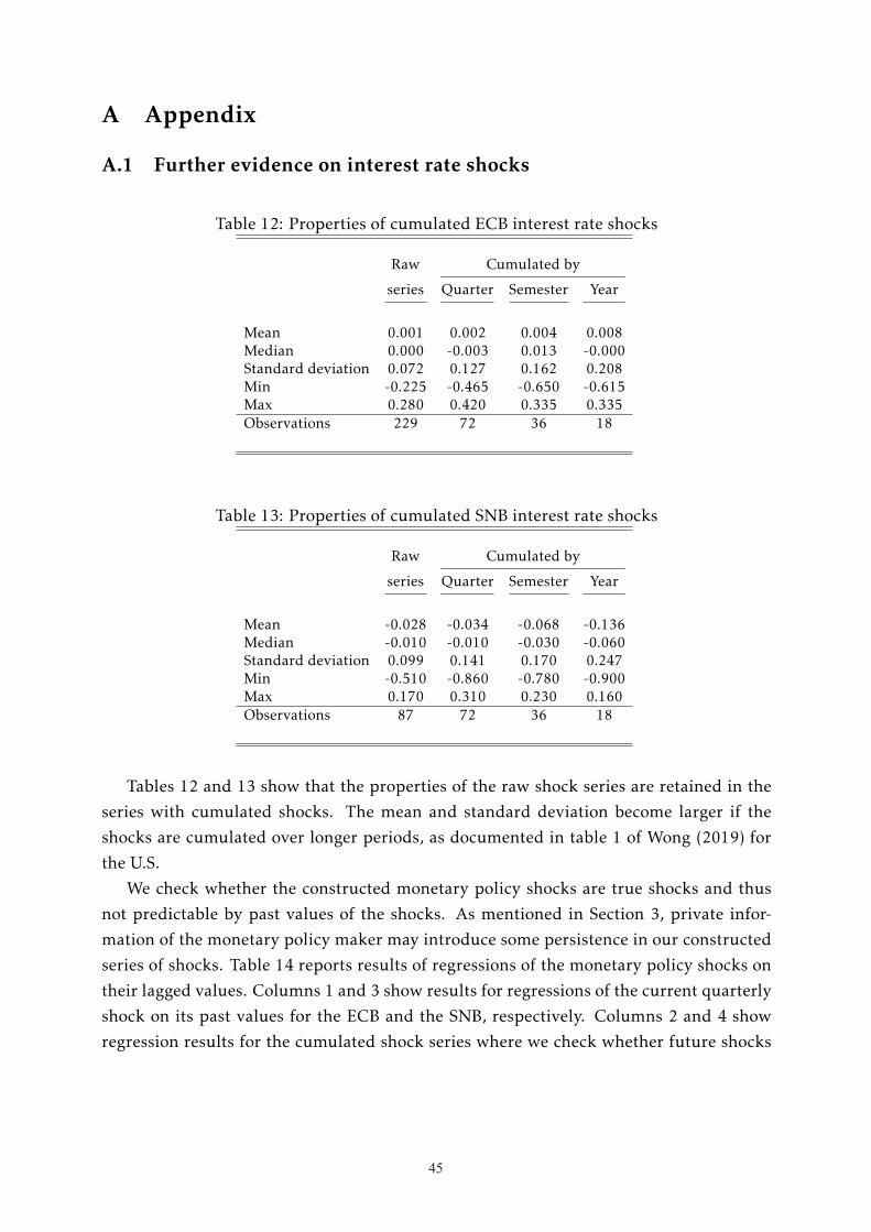
44 45

Kuttner, K. N. (2001). Monetary Policy Surprises and Interest Rates: Evidence from the

Fed Funds Futures Market. Journal of Monetary Economics, 47(3):523–544.

Ma, E. and Zubairy, S. (2021). Homeownership and Housing Transitions: Explaining the

Demographic Composition. International Economic Review.

Nakamura, E. and Steinsson, J. (2014). Fiscal Stimulus in a Monetary Union: Evidence

from US Regions. American Economic Review, 104(3):753–792.

Nakamura, E. and Steinsson, J. (2018). High Frequency Identification of Monetary Non-

Neutrality: The Information Effect. Quarterly Journal of Economics, 133(3):1283–1330.

Piazzesi, M. and Schneider, M. (2016). Housing and Macroeconomics. In Handbook ofMacroeconomics, volume 2, pages 1547–1640. Elsevier.

Ranaldo, A. and Rossi, E. (2010). The Reaction of Asset Markets to Swiss National Bank

Communication. Journal of International Money and Finance, 29:486–503.

Rudebusch, G. D. (1998). Do Measures of Monetary Policy in a VAR Make Sense? Inter-national Economic Review, 39:907–931.

Schularick, M., ter Steege, L., and Ward, F. (2020). Leaning against the Wind and Crisis

Risk. CESifo Working Paper No. 8484.

Slacalek, J., Tristani, O., and Violante, G. L. (2020). Household Balance Sheet Channels

of Monetary Policy: a Back of the Envelope Calculation for the Euro Area. Journal ofEconomic Dynamics and Control, 115(103879).

Soderlind, P. (2010). Reaction of Swiss Term Premia to Monetary Policy Surprises. SwissJournal of Economics and Statistics (SJES), 146(I):385–404.

Voorpostel, M., Tillman, R., Lebert, F., Kuhn, U., Lipps, O., Ryser, V.-A., Antal, E., Monsch,

G.-A., N, D., and Wernli, B. (2017). Swiss Household Panel User Guide (1999-2016).

Wave 18, December 2017. Lausanne: FORS.

Wong, A. (2019). Refinancing and the Transmission of Monetary Policy to Consumption.

Working paper, Mimeograph.

Woodford, M. (2012). Inflation Targeting and Financial Stability. Sveriges Riksbank Eco-nomic Review, (1):7–32.

44

A Appendix

A.1 Further evidence on interest rate shocks

Table 12: Properties of cumulated ECB interest rate shocks

Raw Cumulated by

series Quarter Semester Year

Mean 0.001 0.002 0.004 0.008Median 0.000 -0.003 0.013 -0.000Standard deviation 0.072 0.127 0.162 0.208Min -0.225 -0.465 -0.650 -0.615Max 0.280 0.420 0.335 0.335Observations 229 72 36 18

Table 13: Properties of cumulated SNB interest rate shocks

Raw Cumulated by

series Quarter Semester Year

Mean -0.028 -0.034 -0.068 -0.136Median -0.010 -0.010 -0.030 -0.060Standard deviation 0.099 0.141 0.170 0.247Min -0.510 -0.860 -0.780 -0.900Max 0.170 0.310 0.230 0.160Observations 87 72 36 18

Tables 12 and 13 show that the properties of the raw shock series are retained in the

series with cumulated shocks. The mean and standard deviation become larger if the

shocks are cumulated over longer periods, as documented in table 1 of Wong (2019) for

the U.S.

We check whether the constructed monetary policy shocks are true shocks and thus

not predictable by past values of the shocks. As mentioned in Section 3, private infor-

mation of the monetary policy maker may introduce some persistence in our constructed

series of shocks. Table 14 reports results of regressions of the monetary policy shocks on

their lagged values. Columns 1 and 3 show results for regressions of the current quarterly

shock on its past values for the ECB and the SNB, respectively. Columns 2 and 4 show

regression results for the cumulated shock series where we check whether future shocks

45

46

can be predicted by past values at different horizons. As mentioned in the main text in

Section 3, the results by and large support that our constructed series of the shocks are

not predictable by past values and thus are true shocks.

In our main regression specifications, we cumulate shocks for every year. Figure 5

shows that for these moving sums of the shocks, the autocorrelations are not significant

beyond two quarters. Hence, multicollinearity of the lagged shocks in the regressions is

not a concern.

In Figure 6 we provide evidence that the three-month Euribor is highly correlated with

the midpoint of the ECB policy rates, the rate on the main refinancing operations.

Table 15 shows that the pass-through of policy rate shocks to mortgage interest rates

is stronger for Italy if we restrict the sample to shocks that are positively correlated with

long-term yields. As mentioned in subsection 4.2 in the main text, this suggests that the

pass-through to mortgage rates has been weaker in Italy during the euro-area debt crisis.

Table 14: Regressions of current and future monetary policy shocks on past shocks(1) (2) (3) (4)

ECB, Current quarterly shock ECB, Summed shocks in Q(+1,+4) SNB, Current quarterly shock SNB, Summed shocks in Q(+1,+4)Monetary policy shock, Q(-1) -0.146 -0.190

(-1.16) (-1.52)

Monetary policy shock, Q(-2) -0.128 -0.072(-1.01) (-0.56)

Monetary policy shock, Q(-3) -0.053 0.008(-0.45) (0.06)

Monetary policy shock, Q(-4) 0.068 -0.104(0.59) (-0.87)

Monetary policy shock, sum Q(-1,-4) 0.025 -0.170(0.18) (-1.23)

Monetary policy shock, sum Q(-5,-8) 0.0101 0.028(0.08) (0.19)

Monetary policy shock, sum Q(-9,-12) 0.014 0.275*(0.11) (2.00)

Observations 68 56 68 56R2 0.04 0.00 0.05 0.12

Notes: * p<0.10, ** p<0.05, *** p<0.01. Standard errors in brackets. Dependent variables are indicated atthe top of the respective columns. All regressions include a constant. Current shock refers to the sum ofthe shocks that take place in a given quarter. Sum Q(+1,+4) denotes shocks cumulated over the next fourquarters.

46

46 47

-1.0

0-0

.50

0.00

0.50

1.00

Auto

corre

latio

n co

effic

ient

s of

Sum

Q(-1

;-4)

0 5 10 15 20 25Lags (quarters)

Bartlett's formula for MA(q) 95% confidence bands

ECB

-1.0

0-0

.50

0.00

0.50

1.00

Auto

corre

latio

n co

effic

ient

s of

Sum

Q(-1

;-4)

0 5 10 15 20 25Lags (quarters)

Bartlett's formula for MA(q) 95% confidence bands

SNB

Notes: Correlograms of the moving sum of the quarterly shocks cumulated over a year.

Figure 5: Correlograms of the cumulated shock series

01

23

45

2000

2001

2002

2003

2004

2005

2006

2007

2008

2009

2010

2011

2012

2013

2014

2015

2016

2017

2018

2019

2020

Main Refinancing Operations (MRO) rate3-month Euribor

Correlation = .9901

23

45

3-m

onth

Eur

ibor

0 1 2 3 4 5Main Refinancing Operations (MRO) rate

Sources: Euribor and MRO rates from Thomson Reuters (Y03728 and S245UE). We plot the values at theend of each month for both series.

Figure 6: Euribor and the rate on main refinancing operations (MRO) of the ECB

47

48

Table 15: Pass-through of policy rate shocks to five-year fixed-rate mortgage rates usingshocks positively correlated with long-term yields


Monetary policy shocks, sum M(0) 0.012 −0.073 0.844∗∗∗ †

Monetary policy shocks, sum M(-1) 0.288∗∗∗ 0.361∗ −0.012Monetary policy shocks, sum M(-2) 0.232∗∗ 0.411∗ 0.046

Cum. effect of 25 bp cut −0.133∗∗∗ −0.175∗ −0.219∗∗∗


Monetary policy shocks, sum M(-1) 0.267∗∗∗ 0.396∗∗ −0.012Monetary policy shocks, sum M(-2) 0.261∗∗ 0.406 0.044Monetary policy shocks, sum M(-3) 0.049 0.043 0.034


Sources: Rates of five-year fixed-rate mortgages from the ECB (GermanyMIR.M.DE.B.A2C.O.R.A.2250.EUR.N, Italy MIR.M.IT.B.A2C.O.R.A.2250.EUR.N) and the SNB([email protected]{M,50}) . Notes: Regression of monthly mortgage-rate changes on policy rateshocks cumulated by month. Significance levels: ∗ p < 0.10, ∗∗ p < 0.05, ∗∗∗ p < 0.01. The series arebased on the monthly changes in the rates available for the period 2008M1-2017M12 in Switzerland and2003M1-2017M12 in the euro area. The cumulative effect over three years of a -25 bp shock is computedby multiplying the sum of the coefficients by -0.25.† Regular policy announcements at the SNB take place once a quarter. For the months without anannouncement the value of the shock is zero.

48

48 49

Table 15: Pass-through of policy rate shocks to five-year fixed-rate mortgage rates usingshocks positively correlated with long-term yields



Monetary policy shocks, sum M(-1) 0.288∗∗∗ 0.361∗ −0.012Monetary policy shocks, sum M(-2) 0.232∗∗ 0.411∗ 0.046



Monetary policy shocks, sum M(-1) 0.267∗∗∗ 0.396∗∗ −0.012Monetary policy shocks, sum M(-2) 0.261∗∗ 0.406 0.044Monetary policy shocks, sum M(-3) 0.049 0.043 0.034


Sources: Rates of five-year fixed-rate mortgages from the ECB (GermanyMIR.M.DE.B.A2C.O.R.A.2250.EUR.N, Italy MIR.M.IT.B.A2C.O.R.A.2250.EUR.N) and the SNB([email protected]{M,50}) . Notes: Regression of monthly mortgage-rate changes on policy rateshocks cumulated by month. Significance levels: ∗ p < 0.10, ∗∗ p < 0.05, ∗∗∗ p < 0.01. The series arebased on the monthly changes in the rates available for the period 2008M1-2017M12 in Switzerland and2003M1-2017M12 in the euro area. The cumulative effect over three years of a -25 bp shock is computedby multiplying the sum of the coefficients by -0.25.† Regular policy announcements at the SNB take place once a quarter. For the months without anannouncement the value of the shock is zero.

48

A.2 Robustness of response of housing tenure

A.2.1 Different time windows around the policy announcements

We check robustness of the effect of policy rate shocks on housing tenure transitions if

we use different time windows around the policy announcement. As alternatives to our

benchmark of daily time windows, we use shorter time windows around the announce-

ments, i.e., the six-hour time window used by Corsetti et al. (2020) for constructing inter-

est rate shocks for the ECB, and the 30-minute window used by Gertler and Karadi (2015)

and Nakamura and Steinsson (2018) for constructing interest rate shocks for the Federal

Reserve. For a description of the timing of the policy announcements see Section 3.

Table 16 shows the correlation between shock series that use different time windows

on the days of the monetary policy announcements of the ECB and SNB, respectively.

We compute the correlations for the raw series of shocks (one observation per policy an-

nouncement), and for the series with the shocks cumulated to quarters, semesters or years.

The table shows that our benchmark series for monetary policy shocks in Switzerland is

highly correlated if we use the alternative time windows with correlation coefficients of

0.94 and 0.86 for the shock series based on the six-hour and the 30-minute time window,

respectively. For the euro area, the correlation between our benchmark raw series of the

shocks and the series based on the six-hour time window is 0.7. The correlation between

our benchmark series and the series based on the 30-minute window is smaller at 0.34.

This illustrates that the communication of monetary policy by the ECB requires longer

time windows for constructing interest rate shocks because the very short time window

of 30 minutes does not capture all the new information which is released.

We thus report robustness checks for the euro-area countries Germany and Italy using

the series for monetary policy shocks based on a six-hour time window, as in Corsetti et al.

(2020). For Switzerland, we report robustness results for both the shock series based on

the six-hour and the 30-minute time window.

Table 16 further shows that cumulation of the monetary policy shocks reduces the cor-

relation between the series based on alternative time windows, as shocks partially wash

out when they are cumulated. This is less the case for Switzerland than for the euro area.

Tables 17 and 18 display the results for the effect of the policy shocks on housing

tenure transitions, using the shocks constructed with the alternative time windows men-

tioned above.

49

50

Table 16: Correlation of benchmark with series for interest rate shocks using differenttime windows

ECB SNB

Correlation of benchmark withseries using time windows as in Corsetti et al. (2020) Nakamura and Steinsson (2018) Corsetti et al. (2020) Nakamura and Steinsson (2018)

Raw series 0.695*** 0.337*** 0.944*** 0.857***

Cumulated by... quarter 0.673*** 0.330*** 0.949*** 0.902***... semester 0.434*** 0.150 0.935*** 0.825***... year 0.268 0.251 0.935*** 0.807***

Notes: Significance levels: ∗ p < 0.10, ∗∗ p < 0.05, ∗∗∗ p < 0.01. Correlations of the benchmark with shockseries using different time windows, for the respective raw series of shocks and when cumulated for variousfrequencies.

Table 17: The effect of monetary policy shocks on housing tenure transitions, using thetime window as in Corsetti et al. (2020) for constructing the shocks



Monetary policy shock, sum Q(-1,-4) -0.013 0.453*** -0.061 -0.001 0.033** -0.071***Monetary policy shock, sum Q(-5,-8) -0.009 -0.006 -0.048 -0.003 -0.008** -0.065***Monetary policy shock, sum Q(-9,-12) -0.018 0.192** -0.026 -0.004 0.036** 0.012


Cum. effect (in pp) of 25 bp cut 0.99 -7.97*** 3.37 0.19 -0.76** 3.08***


50

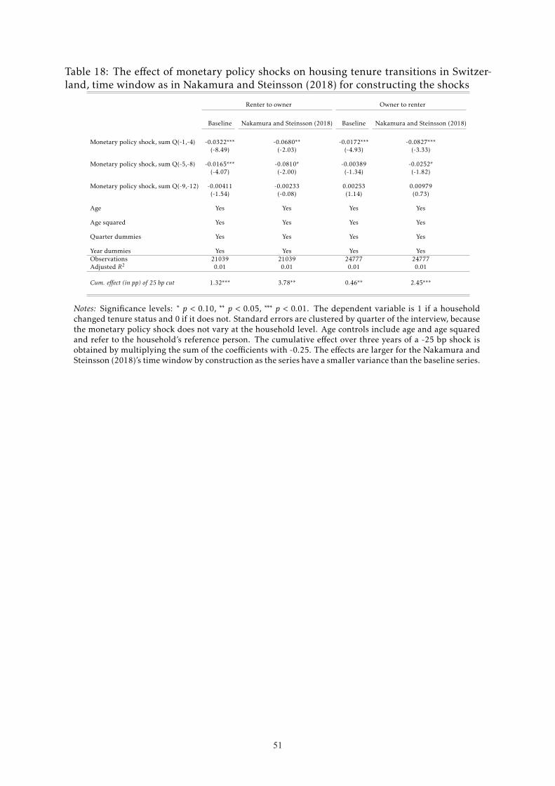
50 51

Table 18: The effect of monetary policy shocks on housing tenure transitions in Switzer-land, time window as in Nakamura and Steinsson (2018) for constructing the shocks


Baseline Nakamura and Steinsson (2018) Baseline Nakamura and Steinsson (2018)

Monetary policy shock, sum Q(-1,-4) -0.0322*** -0.0680** -0.0172*** -0.0827***(-8.49) (-2.03) (-4.93) (-3.33)

Monetary policy shock, sum Q(-5,-8) -0.0165*** -0.0810* -0.00389 -0.0252*(-4.07) (-2.00) (-1.34) (-1.82)

Monetary policy shock, sum Q(-9,-12) -0.00411 -0.00233 0.00253 0.00979(-1.54) (-0.08) (1.14) (0.73)

Age Yes Yes Yes Yes

Age squared Yes Yes Yes Yes

Quarter dummies Yes Yes Yes Yes

Year dummies Yes Yes Yes YesObservations 21039 21039 24777 24777Adjusted R2 0.01 0.01 0.01 0.01

Cum. effect (in pp) of 25 bp cut 1.32*** 3.78** 0.46** 2.45***

Notes: Significance levels: ∗ p < 0.10, ∗∗ p < 0.05, ∗∗∗ p < 0.01. The dependent variable is 1 if a householdchanged tenure status and 0 if it does not. Standard errors are clustered by quarter of the interview, becausethe monetary policy shock does not vary at the household level. Age controls include age and age squaredand refer to the household’s reference person. The cumulative effect over three years of a -25 bp shock isobtained by multiplying the sum of the coefficients with -0.25. The effects are larger for the Nakamura andSteinsson (2018)’s timewindow by construction as the series have a smaller variance than the baseline series.

51

52

A.2.2 Using shocks to long-term yields

Table 19: The effect of monetary policy shocks on housing tenure transitions using five-year government bond yield changes on announcement dates



5y yield change on announcement date, sum Q(-1,-4) -0.020 0.038 -0.058*** 0.005 0.003 -0.023***5y yield change on announcement date, sum Q(-5,-8) -0.031** -0.025 -0.027*** 0.003 -0.001 -0.0045y yield change on announcement date, sum Q(-9,-12) -0.017 0.006 0.008 -0.000 0.004 0.008


Cum. effect (in pp) of 25 bp cut 1.68** -0.25 1.94*** -0.20 -0.07 0.48


52

52 53

A.2.3 Excluding financial crisis years

Table 20: The effect of monetary policy shocks on housing tenure transitions withoutfinancial crises years 2007/08



Monetary policy shock, sum Q(-1,-4) -0.014 0.014 -0.033*** 0.003 -0.012*** -0.019***Monetary policy shock, sum Q(-5,-8) -0.027 0.058* -0.017*** 0.001 0.010*** -0.005Monetary policy shock, sum Q(-9,-12) -0.024* 0.063*** -0.005* 0.001 0.009*** 0.003


Cum. effect (in pp) of 25 bp cut 1.62* -1.69*** 1.38*** -0.14 -0.08** 0.51***


53

54

A.2.4 Excluding periods with negative interest rate policies

Table 21: The effect of monetary policy shocks on housing tenure transitions excludingquarters with a negative interest rate policy (NIRP)



Monetary policy shock, sum Q(-1,-4) -0.017 -0.020** -0.032*** -0.002 -0.003*** -0.017***Monetary policy shock, sum Q(-5,-8) -0.029* 0.040** -0.016*** -0.000 0.016*** -0.003Monetary policy shock, sum Q(-9,-12) -0.024* 0.061*** -0.004 0.004 0.012*** 0.003


Cum. effect (in pp) of 25 bp cut 1.76** -1.01*** 1.29*** -0.06 -0.32*** 0.44**

Notes: Significance levels: ∗ p < 0.10, ∗∗ p < 0.05, ∗∗∗ p < 0.01. The dependent variable is 1 if a householdchanged tenure status and 0 if it does not. Standard errors are clustered by quarter of the interviewfor Germany and Switzerland and by year for Italy, because the monetary policy shock does not vary atthe household level. Age controls include age and age squared and refer to the household’s referenceperson. The cumulative effect over three years of a -25 bp shock is obtained by multiplying the sum of thecoefficients with -0.25. The reported cumulative effects for Italy based on biannual transitions are adjustedto be comparable with those for Germany and Switzerland based on annual transitions. The regressionsexclude periods from Q3, 2014 onward for the euro area (as the ECB deposit facility rate became negativein Q2, 2014) and from Q1, 2015 onward for Switzerland (as the SNB sight deposit rate became negative inQ4, 2014).

54

54 55

A.2.4 Excluding periods with negative interest rate policies

Table 21: The effect of monetary policy shocks on housing tenure transitions excludingquarters with a negative interest rate policy (NIRP)



Monetary policy shock, sum Q(-1,-4) -0.017 -0.020** -0.032*** -0.002 -0.003*** -0.017***Monetary policy shock, sum Q(-5,-8) -0.029* 0.040** -0.016*** -0.000 0.016*** -0.003Monetary policy shock, sum Q(-9,-12) -0.024* 0.061*** -0.004 0.004 0.012*** 0.003


Cum. effect (in pp) of 25 bp cut 1.76** -1.01*** 1.29*** -0.06 -0.32*** 0.44**

Notes: Significance levels: ∗ p < 0.10, ∗∗ p < 0.05, ∗∗∗ p < 0.01. The dependent variable is 1 if a householdchanged tenure status and 0 if it does not. Standard errors are clustered by quarter of the interviewfor Germany and Switzerland and by year for Italy, because the monetary policy shock does not vary atthe household level. Age controls include age and age squared and refer to the household’s referenceperson. The cumulative effect over three years of a -25 bp shock is obtained by multiplying the sum of thecoefficients with -0.25. The reported cumulative effects for Italy based on biannual transitions are adjustedto be comparable with those for Germany and Switzerland based on annual transitions. The regressionsexclude periods from Q3, 2014 onward for the euro area (as the ECB deposit facility rate became negativein Q2, 2014) and from Q1, 2015 onward for Switzerland (as the SNB sight deposit rate became negative inQ4, 2014).

54

A.2.5 Additional lags

Table 22: The effect of monetary policy shocks on housing tenure transitions with addi-tional lags



Monetary policy shock, sum Q(-1,-4) -0.017 -0.024 -0.021** -0.024** -0.035*** -0.043*** -0.001 0.003 -0.003 -0.003* -0.015*** -0.012***Monetary policy shock, sum Q(-5,-8) -0.043** -0.053*** 0.062** 0.104*** -0.021*** -0.038*** 0.001 0.005 0.008 0.011* -0.001 0.005Monetary policy shock, sum Q(-9,-12) -0.034** -0.042** 0.068*** 0.070*** -0.004** -0.034** -0.001 0.005 0.007** 0.008*** 0.001 0.011Monetary policy shock, sum Q(-13,-16) -0.012 0.062*** -0.028* 0.008 0.005* 0.009*Monetary policy shock, sum Q(-17,-20) -0.023 -0.033* -0.004 0.013*Monetary policy shock, sum Q(-21,-24) -0.006 -0.050* -0.006 0.014

Age controls Yes Yes Yes Yes Yes Yes Yes Yes Yes Yes Yes YesQuarter dummies Yes Yes No No Yes Yes Yes Yes No No Yes YesYear dummies Yes Yes No No Yes Yes Yes Yes No No Yes YesLinear trend No No Yes Yes No No No Yes Yes Yes No NoObservations 53,574 53,574 5,026 5,026 18,259 18,259 56,688 56,688 19,775 19,775 21,983 21,983Adjusted R2 0.00 0.00 0.01 0.01 0.01 0.01 0.00 0.00 0.00 0.00 0.01 0.01

Cum. effect (in pp) of 25 bp cut 2.35** 4.00** -1.36** -2.65*** 1.51*** 5.64** 0.03 -0.27 -0.15* -0.26** 0.36** -1.01

Notes: Significance levels: ∗ p < 0.10, ∗∗ p < 0.05, ∗∗∗ p < 0.01. The table shows the results of tenure transitionregressions with additional lags. For Italy, the available degrees of freedom do not allow to include morethan one additional lag. For Germany and Switzerland, the available sample shortens starting with theyear 2006. For Italy, the available sample shortens starting with the year 2003. The dependent variableis 1 if a household changed tenure status and 0 if it does not. Standard errors are clustered by quarter ofthe interview for Germany and Switzerland and by year for Italy, because the monetary policy shock doesnot vary at the household level. Age controls include age and age squared and refer to the household’sreference person. The cumulative effect over three years of a -25 bp shock is obtained by multiplying thesum of the coefficients with -0.25. The reported cumulative effects for Italy based on biannual transitionsare adjusted to be comparable with those for Germany and Switzerland based on annual transitions.

55

56

A.2.6 Additional household controls

Table 23: The effect of monetary policy shocks on housing tenure transitions with addi-tional controls



Monetary policy shock, sum Q(-1,-4) -0.015 -0.021*** -0.029*** 0.002 -0.004 -0.018***Monetary policy shock, sum Q(-5,-8) -0.028** 0.051** -0.013*** 0.001 0.009 -0.008***Monetary policy shock, sum Q(-9,-12) -0.025** 0.068*** -0.002 0.003 0.008** 0.000

Household controls† Yes Yes Yes Yes Yes Yes


Cum. effect (in pp) of 25 bp cut 1.70** -1.21*** 1.10*** -0.13 -0.17 0.66***

Notes: Significance levels: ∗ p < 0.10, ∗∗ p < 0.05, ∗∗∗ p < 0.01. The dependent variable is 1 if a householdchanged tenure status and 0 if it does not. Standard errors are clustered by quarter of the interviewfor Germany and Switzerland and by year for Italy, because the monetary policy shock does not vary atthe household level. Age controls include age and age squared and refer to the household’s referenceperson. The cumulative effect over three years of a -25 bp shock is obtained by multiplying the sum of thecoefficients with -0.25. The reported cumulative effects for Italy based on biannual transitions are adjustedto be comparable with those for Germany and Switzerland based on annual transitions. † Householdcontrols include household size, employment status, civil status, relationship status, gender, domesticnationality and real household income. Household income is gross for Germany and Switterland and netfor Italy.

56

56 57

A.2.7 Non-linear probability models for housing tenure

Table 24: Different specifications for the effect of monetary policy shocks on housingtenure transitions


Probit Logit Probit Logit

Germany Italy Switzerland Germany Italy Switzerland Germany Italy Switzerland Germany Italy Switzerland

Monetary policy shock, sum Q(-1,-4) -0.013 -0.024*** -0.027*** -0.014 -0.023*** -0.026*** 0.003 -0.003** -0.015*** 0.002 -0.003** -0.014***Monetary policy shock, sum Q(-5,-8) -0.022* 0.059** -0.012*** -0.022* 0.056** -0.011*** 0.003 0.007 -0.002 0.002 0.007 -0.002Monetary policy shock, sum Q(-9,-12) -0.022* 0.070*** 0.000 -0.021* 0.069*** 0.001 0.003 0.007*** 0.002 0.003 0.007*** 0.003

Age controls Yes Yes Yes Yes Yes Yes Yes Yes Yes Yes Yes YesQuarter dummies Yes No Yes Yes No Yes Yes No Yes Yes No YesYear dummies Yes No Yes Yes No Yes Yes No Yes Yes No YesLinear trend No Yes No No Yes No No Yes No No Yes NoObservations 67,431 5,677 21,039 67,431 5,677 21,039 71,251 22,219 24,777 71,251 22,219 24,777

Notes: Significance levels: ∗ p < 0.10, ∗∗ p < 0.05, ∗∗∗ p < 0.01. The dependent variable is 1 if a householdchanged tenure status and 0 if it does not. Standard errors are clustered by quarter of the interview forGermany and Switzerland and by year for Italy, because the monetary policy shock does not vary at thehousehold level. Age controls include age and age squared and refer to the household’s reference person.The reported coefficients are marginal effects (and are hence comparable across specifications), computedat the mean. For the computation of the marginal effects in the logit and probit specifications, we set themonetary policy shocks to zero - which is the approximate value of the shocks’ mean.

57

58

A.2.8 Asymmetric effect of positive or negative interest rate shocks?

Table 25: The effect of monetary policy shocks on housing tenure transitions distinguish-ing positive and negative shocks



Monetary policy shock, sum Q(-1,-4) -0.038** 0.047*** -0.066 0.014** -0.003*** -0.073Monetary policy shock, sum Q(-5,-8) -0.038* 0.198*** -0.172 -0.003 0.006*** 0.121Monetary policy shock, sum Q(-9,-12) -0.048** 0.092*** 0.039 0.008 0.025*** -0.056Monetary policy shock, sum Q(-1,-4) × Negative shock 0.036 -0.088*** 0.037 -0.030*** -0.001 0.057Monetary policy shock, sum Q(-5,-8) × Negative shock 0.020 -0.240*** 0.161 -0.001 -0.013*** -0.130Monetary policy shock, sum Q(-9,-12) × Negative shock 0.054** -0.001 -0.049 -0.021** -0.023*** 0.065


Cum. effect (in pp) of 25 bp decrease 0.30 -0.11*** 1.23*** 0.82* 0.12*** 0.38Cum. effect (in pp) of 25 bp increase -3.03** 4.23*** -4.96 0.48 0.35*** -0.18

Notes: Significance levels: ∗ p < 0.10, ∗∗ p < 0.05, ∗∗∗ p < 0.01. The dependent variable is 1 if a householdchanged tenure status and 0 if it does not. Standard errors are clustered by quarter of the interviewfor Germany and Switzerland and by year for Italy, because the monetary policy shock does not vary atthe household level. Age controls include age and age squared and refer to the household’s referenceperson. The cumulative effect over three years of a -25 bp shock is obtained by multiplying the sum ofthe coefficients with -0.25. The reported cumulative effects for Italy based on biannual transitions areadjusted to be comparable with those for Germany and Switzerland based on annual transitions. Notethat the cumulative effect of a 25 bp change can be significant although the individual coefficients are notsignificant because of the covariance of the estimates.

58

58 59

A.2.8 Asymmetric effect of positive or negative interest rate shocks?

Table 25: The effect of monetary policy shocks on housing tenure transitions distinguish-ing positive and negative shocks



Monetary policy shock, sum Q(-1,-4) -0.038** 0.047*** -0.066 0.014** -0.003*** -0.073Monetary policy shock, sum Q(-5,-8) -0.038* 0.198*** -0.172 -0.003 0.006*** 0.121Monetary policy shock, sum Q(-9,-12) -0.048** 0.092*** 0.039 0.008 0.025*** -0.056Monetary policy shock, sum Q(-1,-4) × Negative shock 0.036 -0.088*** 0.037 -0.030*** -0.001 0.057Monetary policy shock, sum Q(-5,-8) × Negative shock 0.020 -0.240*** 0.161 -0.001 -0.013*** -0.130Monetary policy shock, sum Q(-9,-12) × Negative shock 0.054** -0.001 -0.049 -0.021** -0.023*** 0.065


Cum. effect (in pp) of 25 bp decrease 0.30 -0.11*** 1.23*** 0.82* 0.12*** 0.38Cum. effect (in pp) of 25 bp increase -3.03** 4.23*** -4.96 0.48 0.35*** -0.18

Notes: Significance levels: ∗ p < 0.10, ∗∗ p < 0.05, ∗∗∗ p < 0.01. The dependent variable is 1 if a householdchanged tenure status and 0 if it does not. Standard errors are clustered by quarter of the interviewfor Germany and Switzerland and by year for Italy, because the monetary policy shock does not vary atthe household level. Age controls include age and age squared and refer to the household’s referenceperson. The cumulative effect over three years of a -25 bp shock is obtained by multiplying the sum ofthe coefficients with -0.25. The reported cumulative effects for Italy based on biannual transitions areadjusted to be comparable with those for Germany and Switzerland based on annual transitions. Notethat the cumulative effect of a 25 bp change can be significant although the individual coefficients are notsignificant because of the covariance of the estimates.

58

A.2.9 Distinguishing types of monetary policy shocks

Table 26: The effect of monetary policy shocks when conditioning the shocks on stockmarket movements



Interest News Interest News Interest News Interest News Interest News Interest News

Monetary policy shock, sum Q(-1,-4) -0.057** 0.000 0.059* -0.012* -0.037*** -0.101*** -0.010 0.009 0.002 -0.001 -0.025*** -0.043***Monetary policy shock, sum Q(-5,-8) 0.010 -0.022 0.007 0.000 -0.019* -0.053*** -0.034*** 0.016** -0.003 0.001 -0.007 -0.006Monetary policy shock, sum Q(-9,-12) -0.050** -0.010 -0.047 0.030 -0.002 -0.021** -0.008 0.008 0.001 0.002*** 0.007 -0.004

Age controls Yes Yes Yes Yes Yes Yes Yes Yes Yes Yes Yes YesQuarter dummies Yes Yes No No Yes Yes Yes Yes No No Yes YesYear dummies Yes Yes No No Yes Yes Yes Yes No No Yes YesLinear trend No No Yes Yes No No No Yes Yes Yes No NoObservations 67,431 67,431 5,677 5,677 21,039 21,039 71,251 71,251 22,219 22,219 24,777 24,777Adjusted R2 0.00 0.00 0.00 0.00 0.01 0.01 0.00 0.00 0.00 0.00 0.01 0.01

Cum. effect (in pp) of 25 bp cut 2.45* 0.78 -0.25 -0.23 1.47*** 4.38*** 1.29*** -0.82** 0.01 -0.03 0.63* 1.33***

Notes: Significance levels: ∗ p < 0.10, ∗∗ p < 0.05, ∗∗∗ p < 0.01. The table shows the results of separateregressions using either interest shocks or news shocks. Interest shocks are all baseline monetary policyshocks that have the opposite sign as the return of respective the stock market index (EURO STOXX50/SMI) on the announcement date. The remaining baseline shocks are called news shocks. The dependentvariable is 1 if a household changed tenure status and 0 if it does not. Standard errors are clustered byquarter of the interview for Germany and Switzerland and by year for Italy, because the monetary policyshock does not vary at the household level. Age controls include age and age squared and refer to thehousehold’s reference person. The cumulative effect over three years of a -25 bp shock is obtained bymultiplying the sum of the coefficients with -0.25. The reported cumulative effects for Italy based onbiannual transitions are adjusted to be comparable with those for Germany and Switzerland based onannual transitions.

59

60

A.3 Robustness of response of rents and house prices

Table 27: The effect of monetary policy shocks on rents: Germany, by landlord type(1) (2) (3) (4) (5) (6)

All landlord types All landlord types Private companies Private owner Cooperative PublicAll years Years from 2013 Years from 2013 Years from 2013 Years from 2013 Years from 2013

Monetary policy shock, sum Q(-1,-4) -0.0542 0.271 0.451 0.370 1.066** -0.582(-1.14) (0.84) (0.80) (0.99) (2.83) (-0.69)

Monetary policy shock, sum Q(-5,-8) -0.0747 0.233 0.412 0.231 0.594* -0.0637(-1.06) (0.84) (0.87) (0.72) (1.87) (-0.09)

Monetary policy shock, sum Q(-9,-12) -0.117* -0.0102 -0.146 -0.0184 0.194 -0.168(-1.74) (-0.08) (-0.71) (-0.13) (1.44) (-0.56)

Age Yes Yes Yes Yes Yes Yes

Age squared Yes Yes Yes Yes Yes Yes

Quarter dummies Yes Yes Yes Yes Yes Yes

Year dummies Yes Yes Yes Yes Yes YesObservations 70189 21138 2099 12309 3942 1915Adjusted R2 0.01 0.02 0.04 0.03 0.04 0.03

Cum. effect (in percent) of 25 bp cut 6.15* -12.35 -17.92 -14.56 -46.37** 20.34

Notes: Significance levels: ∗ p < 0.10, ∗∗ p < 0.05, ∗∗∗ p < 0.01. The dependent variable is the log of real annualrent expenditures converted to adult-equivalent units using the equivalent scale detailed in Appendix A.5.Standard errors are clustered by quarter of the interview because the monetary policy shock does not varyat the household level. Age controls include age and age squared and refer to the household’s referenceperson. The cumulative effect over three years of a -25 bp shock is obtained by multiplying the sum of thecoefficients with -0.25.

Column 2 of Table 27 shows that a cut of the interest rate reduces rents in Germany in

the sample period since 2013, in which the SOEP contains information the landlord type.

Hence, the pass-through has become qualitatively more similar to Switzerland compared

to our benchmark period (see Table 10, column 3). Some of the effects reported in Table 27

are large. The effects in columns 3, 4 and 5 would be smaller (in absolute terms), and they

are thus less robust than the effect on rents for public housing in column 6, if we used

shocks to yields of five-year government bonds in the regression instead of the interest

rate shocks. Column 6 of Table 27 shows that the pass-through to rents seems to differ forpublic housing.

We check robustness of the results reported in Table 10 if we use the time windows

for constructing monetary policy shocks as in Corsetti et al. (2020) or Nakamura and

Steinsson (2018). The net effect on rents for Italy, reported in the bottom row of Table 28,

column 2, changes sign but is still imprecisely estimated. Otherwise, the results in Table

28 and Table 29 are similar to our benchmark results reported in Table 10, Section 7.

Finally, Table 30 shows that the results, reported in Table 10 in the main text, are

robust if we use shocks to the yields of five-year government bonds instead of policy rate

shocks. The exception is again the effect on rents in Italy which changes sign but it is not

precisely estimated.

60

60 61

Table 28: The effect of monetary policy shocks on rents and house prices, using the timewindow as in Corsetti et al. (2020) for constructing the shocks



Monetary policy shock, sum Q(-1,-4) -0.094** -0.336 0.136*** 0.032 -0.993 -0.024Monetary policy shock, sum Q(-5,-8) -0.069 -0.200* 0.064** -0.048 -0.803*** -0.027Monetary policy shock, sum Q(-9,-12) -0.128 0.223 0.012 -0.228*** 0.812 -0.003

Age controls Yes Yes Yes Yes Yes -Quarter dummies Yes No Yes Yes No YesYear dummies Yes No Yes Yes No YesLinear trend No Yes No No Yes NoObservations 70,189 12,152 22,918 4,135 42,953 60Adjusted R2 0.01 0.02 0.02 0.02 0.04 1.00

Cum. effect (in percent) of 25 bp cut 7.30 7.83 -4.69** 6.10 24.58 1.36

Notes: † Aggregate, quarterly data for Switzerland because no available household-level data. Significancelevels: ∗ p < 0.10, ∗∗ p < 0.05, ∗∗∗ p < 0.01. The dependent variable in columns 1 to 3 is the log of real annualrent expenditures converted to adult-equivalent units using the equivalent scale detailed in Appendix A.5.The dependent variable in columns 4 and 5 is the log of the deflated house price (2010 euros). The depen-dent variable in column 6 is the price index for flats in Switzerland retrieved from the BIS (Property pricesstatistics, referenceQ:CH:0:8:0:2:0:0). Standard errors are clustered by quarter of the interview for Germanyand Switzerland and by year for Italy, because the monetary policy shock does not vary at the householdlevel. Age controls include age and age squared and refer to the household’s reference person. The cumu-lative effect over three years of a -25 bp shock is obtained by multiplying the sum of the coefficients with-0.25.

61

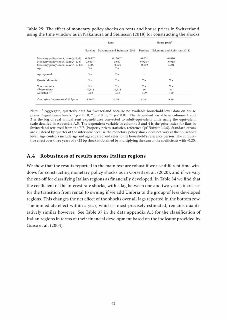
62

Table 29: The effect of monetary policy shocks on rents and house prices in Switzerland,using the time window as in Nakamura and Steinsson (2018) for constructing the shocks

Rent House price†


Monetary policy shock, sum Q(-1,-4) 0.090*** 0.126*** -0.021 -0.010Monetary policy shock, sum Q(-5,-8) 0.050** 0.037 -0.024** -0.015Monetary policy shock, sum Q(-9,-12) -0.000 -0.022 -0.009 0.001Age Yes Yes - -

Age squared Yes Yes - -


Year dummies Yes Yes Yes YesObservations 22,918 22,918 60 60Adjusted R2 0.02 0.02 0.99 1.00

Cum. effect (in percent) of 25 bp cut -3.50*** -3.51** 1.36* 0.60

Notes: † Aggregate, quarterly data for Switzerland because no available household-level data on houseprices. Significance levels: ∗ p < 0.10, ∗∗ p < 0.05, ∗∗∗ p < 0.01. The dependent variable in columns 1 and2 is the log of real annual rent expenditures converted to adult-equivalent units using the equivalentscale detailed in Appendix A.5. The dependent variable in columns 3 and 4 is the price index for flats inSwitzerland retrieved from the BIS (Property prices statistics, reference Q:CH:0:8:0:2:0:0). Standard errorsare clustered by quarter of the interview because the monetary policy shock does not vary at the householdlevel. Age controls include age and age squared and refer to the household’s reference person. The cumula-tive effect over three years of a -25 bp shock is obtained bymultiplying the sum of the coefficients with -0.25.

A.4 Robustness of results across Italian regions

We show that the results reported in the main text are robust if we use different time win-

dows for constructing monetary policy shocks as in Corsetti et al. (2020), and if we vary

the cut-off for classifying Italian regions as financially developed. In Table 34 we find that

the coefficient of the interest rate shocks, with a lag between one and two years, increases

for the transition from rental to owning if we add Umbria to the group of less developed

regions. This changes the net effect of the shocks over all lags reported in the bottom row.

The immediate effect within a year, which is most precisely estimated, remains quanti-

tatively similar however. See Table 37 in the data appendix A.5 for the classification of

Italian regions in terms of their financial development based on the indicator provided by

Guiso et al. (2004).

62

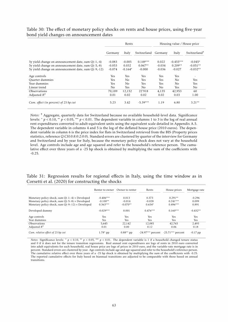
62 63

Table 29: The effect of monetary policy shocks on rents and house prices in Switzerland,using the time window as in Nakamura and Steinsson (2018) for constructing the shocks

Rent House price†


Monetary policy shock, sum Q(-1,-4) 0.090*** 0.126*** -0.021 -0.010Monetary policy shock, sum Q(-5,-8) 0.050** 0.037 -0.024** -0.015Monetary policy shock, sum Q(-9,-12) -0.000 -0.022 -0.009 0.001Age Yes Yes - -

Age squared Yes Yes - -


Year dummies Yes Yes Yes YesObservations 22,918 22,918 60 60Adjusted R2 0.02 0.02 0.99 1.00

Cum. effect (in percent) of 25 bp cut -3.50*** -3.51** 1.36* 0.60

Notes: † Aggregate, quarterly data for Switzerland because no available household-level data on houseprices. Significance levels: ∗ p < 0.10, ∗∗ p < 0.05, ∗∗∗ p < 0.01. The dependent variable in columns 1 and2 is the log of real annual rent expenditures converted to adult-equivalent units using the equivalentscale detailed in Appendix A.5. The dependent variable in columns 3 and 4 is the price index for flats inSwitzerland retrieved from the BIS (Property prices statistics, reference Q:CH:0:8:0:2:0:0). Standard errorsare clustered by quarter of the interview because the monetary policy shock does not vary at the householdlevel. Age controls include age and age squared and refer to the household’s reference person. The cumula-tive effect over three years of a -25 bp shock is obtained bymultiplying the sum of the coefficients with -0.25.

A.4 Robustness of results across Italian regions

We show that the results reported in the main text are robust if we use different time win-

dows for constructing monetary policy shocks as in Corsetti et al. (2020), and if we vary

the cut-off for classifying Italian regions as financially developed. In Table 34 we find that

the coefficient of the interest rate shocks, with a lag between one and two years, increases

for the transition from rental to owning if we add Umbria to the group of less developed

regions. This changes the net effect of the shocks over all lags reported in the bottom row.

The immediate effect within a year, which is most precisely estimated, remains quanti-

tatively similar however. See Table 37 in the data appendix A.5 for the classification of

Italian regions in terms of their financial development based on the indicator provided by

Guiso et al. (2004).

62

Table 30: The effect of monetary policy shocks on rents and house prices, using five-yearbond yield changes on announcement dates



5y yield change on announcement date, sum Q(-1,-4) -0.083 -0.005 0.149*** 0.022 -0.455*** -0.045*5y yield change on announcement date, sum Q(-5,-8) -0.053 0.032 0.067** -0.034 0.209** -0.051**5y yield change on announcement date, sum Q(-9,-12) -0.074 -0.164* -0.000 -0.036 -0.027 -0.032**

Age controls Yes Yes Yes Yes Yes -Quarter dummies Yes No Yes Yes No YesYear dummies Yes No Yes Yes No YesLinear trend No Yes No No Yes NoObservations 70,189 12,152 22’918 4,135 42,953 60Adjusted R2 0.01 0.02 0.02 0.02 0.03 1.00

Cum. effect (in percent) of 25 bp cut 5.23 3.42 -5.39*** 1.19 6.80 3.21**

Notes: † Aggregate, quarterly data for Switzerland because no available household-level data. Significancelevels: ∗ p < 0.10, ∗∗ p < 0.05, ∗∗∗ p < 0.01. The dependent variable in columns 1 to 3 is the log of real annualrent expenditures converted to adult-equivalent units using the equivalent scale detailed in Appendix A.5.The dependent variable in columns 4 and 5 is the log of the deflated house price (2010 euros). The depen-dent variable in column 6 is the price index for flats in Switzerland retrieved from the BIS (Property pricesstatistics, referenceQ:CH:0:8:0:2:0:0). Standard errors are clustered by quarter of the interview for Germanyand Switzerland and by year for Italy, because the monetary policy shock does not vary at the householdlevel. Age controls include age and age squared and refer to the household’s reference person. The cumu-lative effect over three years of a -25 bp shock is obtained by multiplying the sum of the coefficients with-0.25.

Table 31: Regression results for regional effects in Italy, using the time window as inCorsetti et al. (2020) for constructing the shocks


Monetary policy shock, sum Q(-1:-4) × Developed -0.406*** 0.013 0.373 0.291** -0.296Monetary policy shock, sum Q(-5:-8) × Developed -0.100** -0.014 -0.028 0.241*** 0.099Monetary policy shock, sum Q(-9:-12) × Developed 0.363*** -0.070** 0.654* 0.496*** 0.891

Developed dummy -0.029*** 0.001 0.476*** 0.160*** -0.432**


Cum. relative effect of 25 bp cut 1.78* pp 0.88** pp -24.97*** percent -25.71*** percent -0.17 pp

Notes: Significance levels: ∗ p < 0.10, ∗∗ p < 0.05, ∗∗∗ p < 0.01. The dependent variable is 1 if a household changed tenure statusand 0 if it does not for the tenure transition regressions. Real annual rent expenditures are logs of rents in 2010 euro convertedinto adult equivalents for each household, real house price are logs of prices in 2010 euro, and the variable-rate mortgage rate is inpercent. Standard errors are clustered by year. Age controls include age and age squared and refer to the household’s reference person.The cumulative relative effect over three years of a -25 bp shock is obtained by multiplying the sum of the coefficients with -0.25.The reported cumulative effects for Italy based on biannual transitions are adjusted to be comparable with those based on annualtransitions.

63

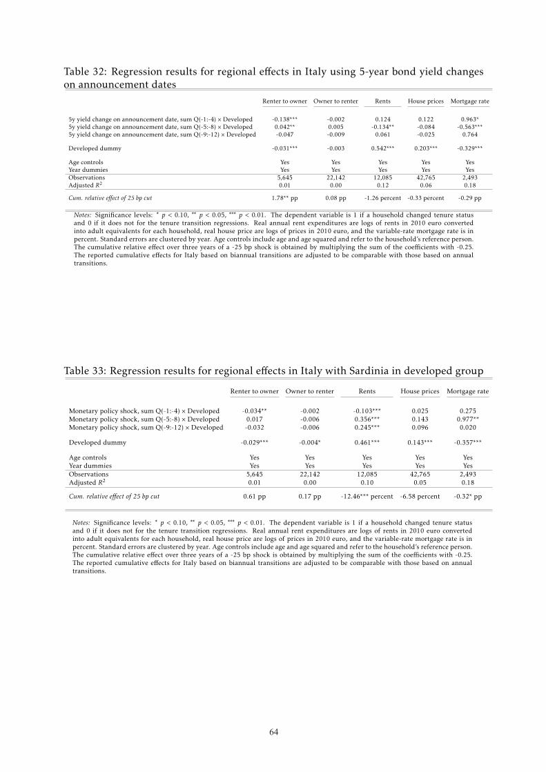
64

Table 32: Regression results for regional effects in Italy using 5-year bond yield changeson announcement dates


5y yield change on announcement date, sum Q(-1:-4) × Developed -0.138*** -0.002 0.124 0.122 0.963*5y yield change on announcement date, sum Q(-5:-8) × Developed 0.042** 0.005 -0.134** -0.084 -0.563***5y yield change on announcement date, sum Q(-9:-12) × Developed -0.047 -0.009 0.061 -0.025 0.764

Developed dummy -0.031*** -0.003 0.542*** 0.203*** -0.329***


Cum. relative effect of 25 bp cut 1.78** pp 0.08 pp -1.26 percent -0.33 percent -0.29 pp


Table 33: Regression results for regional effects in Italy with Sardinia in developed group


Monetary policy shock, sum Q(-1:-4) × Developed -0.034** -0.002 -0.103*** 0.025 0.275Monetary policy shock, sum Q(-5:-8) × Developed 0.017 -0.006 0.356*** 0.143 0.977**Monetary policy shock, sum Q(-9:-12) × Developed -0.032 -0.006 0.245*** 0.096 0.020

Developed dummy -0.029*** -0.004* 0.461*** 0.143*** -0.357***




64

64 65

Table 32: Regression results for regional effects in Italy using 5-year bond yield changeson announcement dates


5y yield change on announcement date, sum Q(-1:-4) × Developed -0.138*** -0.002 0.124 0.122 0.963*5y yield change on announcement date, sum Q(-5:-8) × Developed 0.042** 0.005 -0.134** -0.084 -0.563***5y yield change on announcement date, sum Q(-9:-12) × Developed -0.047 -0.009 0.061 -0.025 0.764

Developed dummy -0.031*** -0.003 0.542*** 0.203*** -0.329***


Cum. relative effect of 25 bp cut 1.78** pp 0.08 pp -1.26 percent -0.33 percent -0.29 pp


Table 33: Regression results for regional effects in Italy with Sardinia in developed group


Monetary policy shock, sum Q(-1:-4) × Developed -0.034** -0.002 -0.103*** 0.025 0.275Monetary policy shock, sum Q(-5:-8) × Developed 0.017 -0.006 0.356*** 0.143 0.977**Monetary policy shock, sum Q(-9:-12) × Developed -0.032 -0.006 0.245*** 0.096 0.020

Developed dummy -0.029*** -0.004* 0.461*** 0.143*** -0.357***




64

Table 34: Regression results for regional effects in Italy with Umbria in less developedgroup


Monetary policy shock, sum Q(-1:-4) × Developed -0.068*** -0.004 -0.075** 0.034 0.395**Monetary policy shock, sum Q(-5:-8) × Developed 0.093* -0.002 0.368*** 0.111 0.427Monetary policy shock, sum Q(-9:-12) × Developed -0.009 -0.003 0.206*** 0.110 0.171

Developed dummy -0.022*** -0.000 0.532*** 0.200*** -0.400***


Cum. effect of 25 bp cut -0.19 pp 0.12 pp -12.47*** percent -6.37 percent -0.25 pp

Notes: Significance levels: ∗ p < 0.10, ∗∗ p < 0.05, ∗∗∗ p < 0.01. The dependent variable is 1 if a household changed tenure status and 0if it does not for the tenure transition regressions. Real annual rent expenditures are logs of rents in 2010 euro converted into adultequivalents for each household, real house price are logs of prices in 2010 euro, and the variable-rate mortgage rate is in percent.Standard errors are clustered by year. Age controls include age and age squared and refer to the household’s reference person.The cumulative relative effect over three years of a -25 bp shock is obtained by multiplying the sum of the coefficients with -0.25.The reported cumulative effects for Italy based on biannual transitions are adjusted to be comparable with those based on annualtransitions.

A.5 Data appendix

The German Socioeconomic Panel (SOEP), the Swiss Household Panel (SHP) and the Ital-

ian Survey on Household Income and Wealth (SHIW) are unbalanced household panels.

Households are interviewed once a year in the SOEP and SHP and every other year in

the SHIW. The SOEP contains information on households since 1990, the SHP since 1999,

and the SHIW since 1977. For all three countries, we use the data on households in the

time period 2000-2016 together with the data series which we constructed for the mone-

tary policy shocks. The summary statistics are reported for the sample period 2002-2016,

which is used in our estimations because monetary policy shocks enter with lags in the

estimated specifications.

For the household-level data in all three countries, our constructed sample consists of

households for which the following variables were recorded: housing tenure (renter or

owner), age, household size (number of people), civil status (married or not as well as in a

partnership or not), working status (yes or no), the interviewee’s gender, nationality and

region, and household income. The SOEP and SHP provide information on household

gross income, which includes labor earnings, capital income, pensions and (government)

transfers. We keep households in the sample which report non-negative household in-

come. In the SHIW, the reported net income includes transfers between households so

that net income can be negative if households make a transfer. Thus, we keep the few

households in the sample that report negative net income. We further keep households

whose interviewee is the household head (or partner), and we focus on household heads

65

66

with an age between 25 and 84. This covers ages at which most households have finished

full-time education, have entered the labor market or are retired. The constructed sample

contains 138,682, 45,816 and 27,896 households, respectively, for the SOEP, the SHP and

the SHIW in the sample period used for the estimations.

We now discuss for each country how we obtain information on the other variables

used in the estimations. For Germany, data on rents, net worth and an approximated

house price are available at the household-level in the SOEP. Households report rent ex-

penditure (annualized and net of utility expenditure) and net worth (total wealth net of

debt). We approximate house prices using the (annualized) mortgage expenditure re-

ported in the data. This expenditure contains both amortization and interest payments,

which cannot be distinguished in the data. We approximate house prices for households

who moved into their current property in the previous two years because these house-

holds are less likely to have altered their initial mortgage contract, and the purchase price

of their home reflects current economic conditions. We assume mortgage amortization

over a typical 25-year period and a loan-to-value ratio of 50%, which corresponds to the

average loan-to-value ratio of German mortgagors, aged 36-45 and thus with relatively

new mortgages, in the 2014 wave of the Household Finance and Consumption Survey

(HFCS). We further use the mortgage rate for the year in which the household moved in.

Specifically, we use the annualized agreed mortgage rate for Germany provided by the

ECB (key: 124.MIR.M.DE.B.A2C.AM.R.A.2250.EUR.N), which is the agreed interest rate

for new mortgages to the household sector.

We assume constant mortgage payments over time as in the typical mortgage contract

observed in Germany.33 Because mortgage payments consist of amortization and interest

payments, the amortization payment At of a household, for a mortgage Dt in period t and

a fixed mortgage interest rate i, is given by:

At =(

1(1+ i)t+1 − 1

)Dt . (A.1)

The mortgage changes over time due to amortization: Dt+1 =Dt−At . The interest payment

is iDt , and the share of mortgage payments used for servicing the interest is st =iDt

At+iDt.

The amortization rate is defined as at =AtDt

so that Dt+1 =Dt(1− at).We use the mortgage payments reported by a household in the SOEP, multiplied by

the share st , to retrieve the interest payment at the household level, and we obtain the

current mortgage value by dividing this interest payment by the mortgage interest rate.

We then back out the initial mortgage value at purchase by adding the amortization pay-

33The estimation results based on the approximated house prices are unchanged if we assume linearamortization.

66

66 67

with an age between 25 and 84. This covers ages at which most households have finished

full-time education, have entered the labor market or are retired. The constructed sample

contains 138,682, 45,816 and 27,896 households, respectively, for the SOEP, the SHP and

the SHIW in the sample period used for the estimations.

We now discuss for each country how we obtain information on the other variables

used in the estimations. For Germany, data on rents, net worth and an approximated

house price are available at the household-level in the SOEP. Households report rent ex-

penditure (annualized and net of utility expenditure) and net worth (total wealth net of

debt). We approximate house prices using the (annualized) mortgage expenditure re-

ported in the data. This expenditure contains both amortization and interest payments,

which cannot be distinguished in the data. We approximate house prices for households

who moved into their current property in the previous two years because these house-

holds are less likely to have altered their initial mortgage contract, and the purchase price

of their home reflects current economic conditions. We assume mortgage amortization

over a typical 25-year period and a loan-to-value ratio of 50%, which corresponds to the

average loan-to-value ratio of German mortgagors, aged 36-45 and thus with relatively

new mortgages, in the 2014 wave of the Household Finance and Consumption Survey

(HFCS). We further use the mortgage rate for the year in which the household moved in.

Specifically, we use the annualized agreed mortgage rate for Germany provided by the

ECB (key: 124.MIR.M.DE.B.A2C.AM.R.A.2250.EUR.N), which is the agreed interest rate

for new mortgages to the household sector.

We assume constant mortgage payments over time as in the typical mortgage contract

observed in Germany.33 Because mortgage payments consist of amortization and interest

payments, the amortization payment At of a household, for a mortgage Dt in period t and

a fixed mortgage interest rate i, is given by:

At =(

1(1+ i)t+1 − 1

)Dt . (A.1)

The mortgage changes over time due to amortization: Dt+1 =Dt−At . The interest payment

is iDt , and the share of mortgage payments used for servicing the interest is st =iDt

At+iDt.

The amortization rate is defined as at =AtDt

so that Dt+1 =Dt(1− at).We use the mortgage payments reported by a household in the SOEP, multiplied by

the share st , to retrieve the interest payment at the household level, and we obtain the

current mortgage value by dividing this interest payment by the mortgage interest rate.

We then back out the initial mortgage value at purchase by adding the amortization pay-

33The estimation results based on the approximated house prices are unchanged if we assume linearamortization.

66

ments to the current mortgage value. We divide the current mortgage value by (1− at) forhouseholds who moved in last year, and by (1− at)(1− at−1) for households who moved in

two years ago. Dividing the initial mortgage value by the loan-to-value ratio of 50%, we

obtain the approximated house value. The average (median) approximated house value

amounts to EUR 206,293 (178,620) and is thus in the ballpark of the values reported by

households in the Household Finance and Consumption Survey (HFCS) for Germany in

2014. Given that we need information on house values before and after the monetary pol-

icy shocks, we cannot use the survey information on house values in the HFCS directly for

our analysis because that survey has been conducted only every three years since 2010.

For Switzerland, we do not have household-level measures on house values and net

worth. We also do not know which households are new homeowners in the Swiss house-

hold budget survey (Haushaltsbudgeterhebung or HABE), which contains information on

mortgage expenditures, so that we cannot apply the approximation of house prices dis-

cussed for the SOEP above. Thus, as mentioned in the main text, we use aggregate-level

house prices for Switzerland. For expenditures on housing rents, we use household-level

data from the HABE. The HABE is a repeated cross-sectional data set. It contains data on

detailed household income and expenditure items between 2000Q1 and 2017Q4 and is

used for the national CPI calculations. We construct the sample for the HABE, proceed-

ing analogously as before for the SOEP, SHP and SHIW, by keeping households whose

interviewee is the reference person (the household head) and is aged between 25 and 84.

We further keep households which report positive gross income, mandatory payments

(which include taxes and mandatory health insurance), disposable income (income mi-

nus mandatory payments), consumption expenditure and rent. To contain the effect ofpotential outliers, we trim the sample by keeping households which report a gross saving

rate (measured as disposable income minus expenditure, divided by disposable income)

between the first and 99th percentiles in a given interview year. The final sample used for

the estimation contains 22,918 renters.

For Italy, the information on house prices is based on the self-reported house value

provided by households in the SHIW. Specifically, households are asked: “In your opinion,

how much is your house/flat worth (unoccupied)? In other words, what price could you

ask for it today (including any cellar, garage or attic)? Please give your best estimate.” For

rents, we use reported annual rent payments. In order to identify households, who have

not moved between survey years, we restrict the sample to those renters who provide the

same construction year of their flat/house for consecutive survey years. For net worth, we

use the definition provided in the SHIW, which is the value of real assets plus the value

of financial assets minus the value of financial liabilities. The median net worth for each

transition group is reported in Table 6, and the median net worth for each of these groups

67

68

by region is shown in Table 38.

For all three considered countries, we convert the series for rental expenditures to

adult-equivalent units by using the equivalent scale of Fernandez-Villaverde and Krueger

(2007) in Table 1, column 7 (p. 554). For households with more than five persons, the

scale is increased by 0.3 per additional person which equals the increment for the fifth

person in Fernandez-Villaverde and Krueger (2007). When indicated, the series are de-

flated by using the annual nationwide CPI with 2010 as the base year. For Germany and

Switzerland we use the series with the FRED codes DEUCPIALLMINMEI and CHECPI-ALLMINMEI, respectively. For Italy, we use the consumption deflator provided in the

SHIW from Istat.

In Tables 35 to 39 we provide further descriptive evidence. Tables 35 and 36 show

that some household characteristics are different across language groups in Switzerland,

whether we classify language groups using information on both the reported mother

tongue and the location of residence in Table 35, or using only information on the re-

ported mother tongue in Table 36. For instance, Italian-speaking households have lower

income across all housing tenure groups. Given these differences, we control for income

as well as some other household characteristics, when we analyze the effect of interest rateshocks on housing tenure transitions across Swiss language groups in Section 6.

Table 37 shows how we classify Italian regions in terms of their financial development

based on the indicator provided by Guiso et al. (2004). We use the binary classification

to construct the spread in the mortgage rates between regions that are more and less

financially developed. In Tables 33 and 34 in Appendix A.2, we provide robustness checks

if we assign the marginal regions, Umbria or Sardinia, to the respective other category.

Table 38 provides summary statistics for the subpopulations that change, or do not

change, housing tenure status in the Italian regions with a different degree of financial

development. Table 38 shows that the differences across the subpopulations discussed in

the main text for Table 6, Section 5, also hold for the two types of Italian regions. The mi-

nor differences in the total sample size compared to Table 6 result from some households

that we drop because they change region type.

Table 39 shows how key characteristics in the housing and mortgage market differacross Italian regions with different financial development.

68

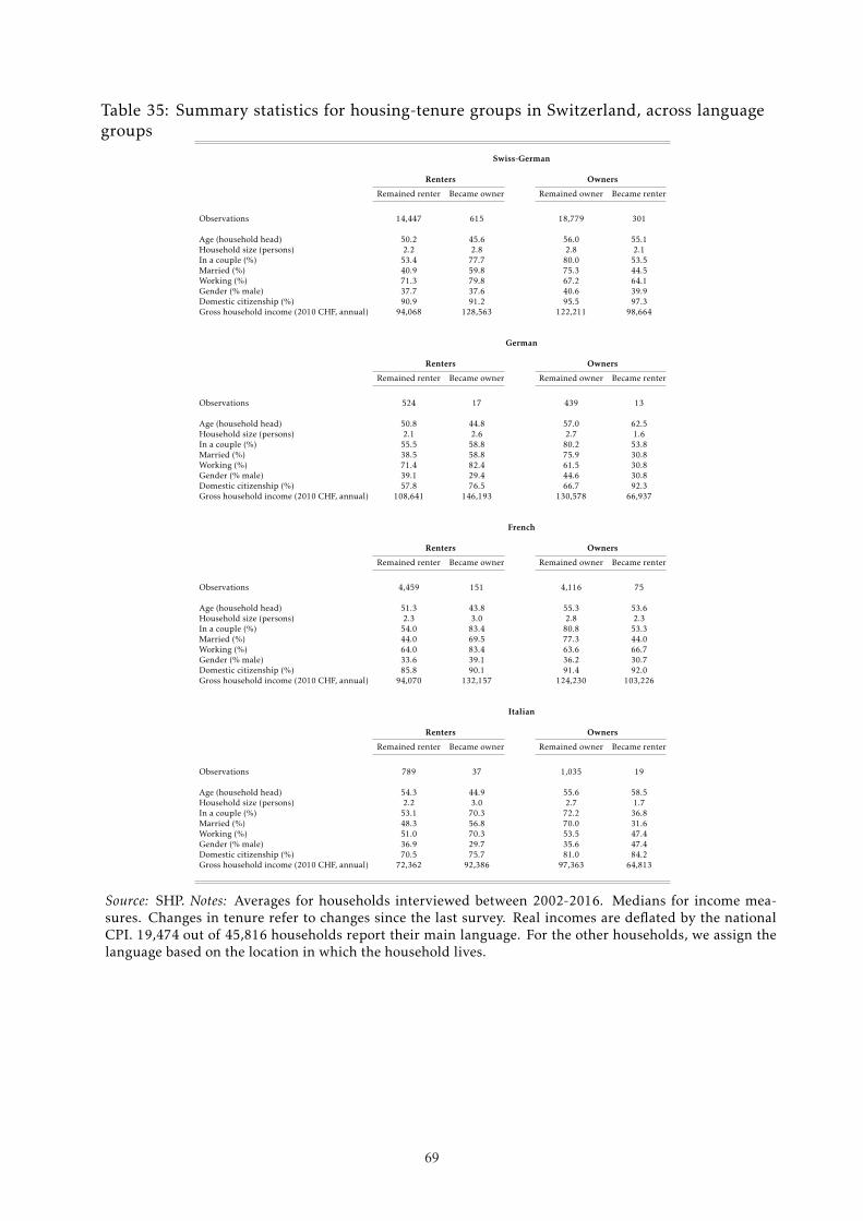
68 69

Table 35: Summary statistics for housing-tenure groups in Switzerland, across languagegroups

Swiss-German

Renters XXX Owners


Observations 14,447 615 18,779 301


German

Renters XXX Owners


Observations 524 17 439 13


French

Renters XXX Owners


Observations 4,459 151 4,116 75


Italian

Renters XXX Owners


Observations 789 37 1,035 19


Source: SHP. Notes: Averages for households interviewed between 2002-2016. Medians for income mea-sures. Changes in tenure refer to changes since the last survey. Real incomes are deflated by the nationalCPI. 19,474 out of 45,816 households report their main language. For the other households, we assign thelanguage based on the location in which the household lives.

69

70

Table 36: Summary statistics for housing-tenure groups in Switzerland, across groups ofreported mother tongue

Swiss-German

Renters XXX Owners


Observations 4’153 163 5’976 91

Age (household head) 52.9 46.3 56.4 57.3Household size (persons) 2.1 2.7 2.7 2.1In a couple (%) 52.8 79.1 78.8 50.6Married (%) 44.6 62.6 74.5 49.5Working (%) 69.1 76.1 67.6 54.9Gender (% male) 39.5 39.3 45.1 42.9Domestic citizenship (%) 95.5 95.7 98.2 100.0Gross household income (2010 CHF, annual) 94’355 123’357 123’330 96’774

German

Renters XXX Owners




French

Renters XXX Owners


Observations 1’519 62 1’738 37


Italian

Renters XXX Owners




Source: SHP.Notes: Averages for households interviewed between 2002-2016. Medians for incomemeasures.Changes in tenure refer to changes since the last survey. Real incomes are deflated by the national CPI.The sample consists of 19,474 (out of 45,816) households that report their main language. The descriptivestatistics for German speakers coincide with those in the previous table by construction because the locationof residence in Switzerland implies assignments only to the other three language groups.

70

70 71

Table 37: Regional split for Italy based on the normalized measure of financial develop-ment in Guiso et al. (2004), table 2.

Region Measure of financial development Classification

Marche 0.59Liguria 0.59Emilia - Romagna 0.52Veneto 0.52Piedmont 0.47 DevelopedTrentino - Alto Adige 0.46Lombardy 0.44Friuli - Venezia Giulia 0.41Umbria 0.40

Sardinia 0.37Tuscany 0.36Abruzzo 0.36Basilicata 0.35Molise 0.25Sicily 0.21 Less developedApulia 0.17Lazio 0.07Campania 0.03Calabria 0.00

Table 38: Summary statistics for housing-tenure groups across Italian regions

Developed Less developed

Renters Owners Renters Owners

Remained renter Became owner Remained owner Became renter Remained renter Became owner Remained owner Became renter

Observations 2,756 219 11,746 155 2,417 253 10,084 157

Age (household head) 55.1 54.1 60.3 57.1 56.6 54.4 60.4 56.4Household size (persons) 2.3 2.2 2.5 1.9 2.8 2.7 2.7 2.0In a couple (%) 52.2 51.1 70.9 36.8 63.4 64.4 70.7 41.4Married (%) 51.9 48.9 70.2 36.1 62.0 63.2 70.3 39.5Working (%) 53.3 58.4 41.3 49.0 35.9 47.0 36.7 47.1Gender (% male) 53.9 55.3 63.0 53.5 51.2 60.1 58.1 50.3Birth region domestic (%) 81.4 91.3 97.5 89.7 93.9 96.8 98.9 98.1Net household income 19,098 30,818 36,191 16,954 14,920 22,235 27,374 15,600(2010 EUR, annual)Net worth 6,616 178,652 256,141 8,230 2,941 144,584 202,317 3,197(2010 EUR)

Sources: SHIW (Italy). Notes: Averages for households interviewed between 2002-2016. Medians for incomeand net worth. Changes in tenure refer to changes since the last survey. Real incomes and net worths aredeflated by the national CPI.

71

72

Table 39: Housing and mortgages across Italian regions

Developed Less developed

Homeownership rate (%) 78.3 (0.5) 80.7 (0.5)Incidence of mortgagors (as % owners) 17.5 (0.5) 14.2 (0.5)Incidence of mortgagors (as % new owners) 23.1 (6.8) 16.1 (5.0)Flexible rate mortgagors (as % of mortagors) 38.6 (1.4) 22.0 (1.3)

Sources: SHIW. Notes: Standard errors in parentheses. The statistics are based on the representative sampleyears 2014/2016 to be comparable with the aggregate statistics in Table 1 in the main text. New owners arerenters who became owners between the last and the current survey wave.

A.6 Annualization of the biannual transition probabilities for Italy

For completeness, we discuss how we obtain the annual transition probabilities based on

information on the biannual transition probabilities. We denote the annual transition

matrix by T1 and the biannual transition matrix by T2 with

T1 =

Renter Owner( )Renter (1− p) p

Owner q (1− q), T2 =

Renter Owner( )Renter (1−P) P

Owner Q (1−Q).

Observing that

T2 = T12 =

(1− p)(1− p) + pq (1− p)p + p(1− q)q(1− p) + (1− q)q qp + (1− q)(1− q)

,

we obtain a system of two equations which maps the annual transition probabilities p

and q into the corresponding biannual transition probabilities P and Q:

P = (1− p)p + p(1− q), (A.2)

Q = (1− q)q + q(1− p). (A.3)

The probabilities 1−P, 1−Q, 1−p and 1−q result from the property that probabilities

in each row of the transition matrices have to sum to one.

Solving equations (A.2) and (A.3) for p and q, respectively, we obtain

72

72 73

p =2− q2−

√(2− q)2

4−P, (A.4)

q =2− p2−

√(2− p)2

4−Q, (A.5)

where we only consider the sign of the root for which 0 ≤ p ≤ 1 and 0 ≤ q ≤ 1.

For annual transitions across housing tenure states that are small, (2 − x)/2 ≈ 1 for

x = p,q, and we obtain the closed form solutions

p ≈ 1−√1−P, (A.6)

q ≈ 1−√1−Q. (A.7)

In Figure 4 we annualize the biannual flows using equations (A.6) and (A.7), respec-

tively. A first-order Taylor approximation of (A.6) and (A.7) implies, as usual, that

p ≈ P2and q ≈ Q

2, (A.8)

if biannual transition probabilities are small. We find that the approximation implies

negligible approximation error in our application. We thus use (A.8) to annualize the

cumulative effects of 25 bp rate cuts for the housing-tenure regressions in Italy.

73

Recent SNB Working Papers

2021-06 WinfriedKoeniger,BenediktLennartz, Marc-Antoine Ramelet: On the transmission of monetary policy to the housing market

2021-05 RomainBaeriswyl,LucasFuhrer,PetraGerlach-Kristen, Jörn Tenhofen: The dynamics of bank rates in a negative-rate environment – the Swiss case

2021-04 RobertOleschak: Financialinclusion,technologyandtheirimpacts onmonetaryandfiscalpolicy:theoryandevidence

2021-03 DavidChaum,ChristianGrothoff,ThomasMoser: How to issue a central bank digital currency

2021-02 JensH.E.Christensen,NikolaMirkov: The safety premium of safe assets

2021-01 TillEbner,ThomasNellen,JörnTenhofen: The rise of digital watchers

2020-25 LucasMarcFuhrer,Marc-AntoineRamelet, Jörn Tenhofen: Firms‘participationintheCOVID-19loanprogramme

2020-24 BasilGuggenheim,SébastienKraenzlin, Christoph Meyer: (In)Efficienciesofcurrentfinancialmarket infrastructures–acallforDLT?

2020-23 MiriamKoomen,LaurenceWicht: Demographics,pensionsystems,andthecurrent account:anempiricalassessmentusingtheIMF current account model

2020-22 YannicStucki,JacquelineThomet: AneoclassicalperspectiveonSwitzerland’s1990s stagnation

2020-21 FabianFink,LukasFrei,OliverGloede: Short-term determinants of bilateral exchange rates: A decomposition model for the Swiss franc

2020-20 LaurenceWicht: A multi-sector analysis of Switzerland’s gains from trade

2020-19 TerhiJokipii,RetoNyffeler,StéphaneRiederer: ExploringBIScredit-to-GDPgapcritiques:the Swiss case

2020-18 EnzoRossi,VincentWolff: Spillovers to exchange rates from monetary and macroeconomic communications events

2020-17 InDoHwang,ThomasLustenberger,EnzoRossi: Doescommunicationinfluenceexecutives’opinion ofcentralbankpolicy?

2020-16 PeterKugler,SamuelReynard: Money,inflationandthefinancialcrisis:thecaseof Switzerland

2020-15 SébastienKraenzlin,ChristophMeyer,ThomasNellen: COVID-19andregionalshiftsinSwissretailpayments

2020-14 ChristianGrisse: Lower bound uncertainty and long-term interest rates

2020-13 AngelaAbbate,SandraEickmeier,EstebanPrieto: Financialshocksandinflationdynamics

2020-12 ToniBeutler,MatthiasGubler,SimonaHauri, Sylvia Kaufmann: Bank lending in Switzerland: Capturing cross-sectional heterogeneity and asymmetry over time

2020-11 SophieAltermatt,SimonBeyeler: Shallwetwist?

on the transmission of monetary policy to the housing market

Documents